Integration of a Star Tracker and Inertial Sensors Using ...

Air Force Institute of TechnologyAFIT Scholar

Theses and Dissertations Student Graduate Works

9-18-2014

Integration of a Star Tracker and Inertial SensorsUsing an Attitude UpdateHumood Alkhaldi

Follow this and additional works at: https://scholar.afit.edu/etd

This Thesis is brought to you for free and open access by the Student Graduate Works at AFIT Scholar. It has been accepted for inclusion in Theses andDissertations by an authorized administrator of AFIT Scholar. For more information, please contact [email protected].

Recommended CitationAlkhaldi, Humood, "Integration of a Star Tracker and Inertial Sensors Using an Attitude Update" (2014). Theses and Dissertations. 562.https://scholar.afit.edu/etd/562

https://scholar.afit.edu?utm_source=scholar.afit.edu%2Fetd%2F562&utm_medium=PDF&utm_campaign=PDFCoverPages

https://scholar.afit.edu/etd?utm_source=scholar.afit.edu%2Fetd%2F562&utm_medium=PDF&utm_campaign=PDFCoverPages

https://scholar.afit.edu/graduate_works?utm_source=scholar.afit.edu%2Fetd%2F562&utm_medium=PDF&utm_campaign=PDFCoverPages

https://scholar.afit.edu/etd?utm_source=scholar.afit.edu%2Fetd%2F562&utm_medium=PDF&utm_campaign=PDFCoverPages

https://scholar.afit.edu/etd/562?utm_source=scholar.afit.edu%2Fetd%2F562&utm_medium=PDF&utm_campaign=PDFCoverPages

mailto:[email protected]

INTEGRATION OF A STAR TRACKER AND INERTIAL SENSORS USING AN ATTITUDE UPDATE

THESIS SEPTEMBER 2014

Humood Alkhaldi, Captain, RSAF

AFIT-ENG-T-14-S-16

DEPARTMENT OF THE AIR FORCE

AIR UNIVERSITY

AIR FORCE INSTITUTE OF TECHNOLOGY

Wright-Patterson Air Force Base, Ohio

DISTRIBUTION STATEMENT A. APPROVED FOR PUBLIC RELEASE; DISTRIBUTION UNLIMITED.

The views expressed in this thesis are those of the author and do not reflect the official policy or position of the United States Air Force, Department of Defense, or the United States Government. This material is declared a work of the U.S. Government and is not subject to copyright protection in the United States.

AFIT-ENG-T-14-S-16


THESIS

Presented to the Faculty

Department of Electrical and Computer Engineering

Graduate School of Engineering and Management

Air Force Institute of Technology

Air University

Air Education and Training Command

In Partial Fulfillment of the Requirements for the

Degree of Master of Science in Electrical Engineering

Humood Alkhaldi, BS

Captain, RSAF

September 2014

DISTRIBUTION STATEMENT A. APPROVED FOR PUBLIC RELEASE; DISTRIBUTION UNLIMITED.

AFIT-ENG-T-14-S-16


Humood Alkhaldi, BS

Captain, RSAF

Approved:

______________//signed//_____________ 19 Aug, 2014 John F. Raquet, PhD (Chairman) Date ______________//signed//_____________ 19 Aug, 2014 Meir Pachter, PhD (Member) Date ______________//signed//_____________ 19 Aug, 2014 Kyle Kauffman, PhD (Member) Date

iv

AFIT-ENG-T-14-S-16

Abstract

The Global Positioning System (GPS) is widely used in most of the military and

civilian applications because of its precision navigation capability. Unfortunately, GPS is

not available in all environments (e.g., indoors, under sea, underground, or jamming

environment). The motivation of this research is to address the limitations of GPS by

using star trackers as an attitude update to an inertial navigation system (INS).

Commercial, tactical, and navigation grade INS are modeled and simulated with

measurements from GPS, star tracker, and barometer. GPS measurements are used to

update the INS position and velocity for a small duration in the beginning of the vehicle’s

flight time. Star tracker and barometer measurements are used to update the INS attitude

and altitude, respectively. This research uses a Linear Kalman Filter as a recursive

estimation system, to estimate the INS errors (i.e. position, velocity, tilts, accelerometer

bias, gyroscope bias, and barometer bias) using the three types of measurement updates.

The simulation results show that the star tracker was able to improve the performance of

the commercial and tactical grades INS, for any duration of the vehicle’s flight time.

Also, the improvement in the performance of the navigation grade INS was not

significant until the vehicle’s flight time was more than approximately 1000 seconds.

Also, the research shows the performance impact on the three INS grades when using

different star tracker accuracies.

v

Acknowledgments

I would like to thank my parents and my brothers for their priers and support

throughout my thesis. Also, I would like to thank my advisor Dr. John Raquet for all the

guidance and knowledge I got from him. In addition, I thank my thesis committee

members, Dr. Meir Pachter and Dr. Kyle Kauffman for their teachings throughout my

courses and thesis. Finally, I thank my friend, 1Lt. Muflih Alqahtani for his support and

friendship through my thesis time.

Humood Alkhaldi

vi

Table of Contents

Page

Abstract .............................................................................................................................. iv

Acknowledgments .............................................................................................................. .v

List of Figures .................................................................................................................... ix

List of Tables .................................................................................................................... xii

I. Introduction ........................................................................................................... 1

1.1 Problem Definition ................................................................................ 2

1.2 Research Contributions ......................................................................... 3

1.3 Thesis Outline ....................................................................................... 3

II. Mathematical Background ................................................................................... 5

2.1 Inertial Navigation System .................................................................... 5

2.2 Direction Cosine Matrix ........................................................................ 6

2.3 Reference Frames .................................................................................. 7

2.3.1 Earth-Centered Inertial Frame ................................................ 8

2.3.2 Earth-Centered Earth-Fixed Frame ....................................... 8

2.3.3 Navigation Frame ................................................................... 8

2.3.4 Body Frame ............................................................................ 9

2.3.5 Sensor Frame ........................................................................ 10

2.4 The WGS-84 Coordinate System ........................................................ 11

2.5 Star Trackers ....................................................................................... 12

vii

Page

2.6 Kalman filter ....................................................................................... 14

2.6.1 Linear Kalman Filter ........................................................... 15

2.6.2 Unscented Kalman Filter ...................................................... 17

2.7 Previous Work .................................................................................... 18

2.7.1 Correction Technique for Velocity and Position Errors of

Inertial Navigation System by Celestial Observations ....... 18

2.7.2 Alternate of GPS for Ballistic Vehicle Navigation ............. 20

2.7.3 Compass Star Tracker for GPS-Like Applications ............. 21

2.8 Chapter Summary ................................................................................ 25

III. Methodology .................................................................................................... 26

3.1 System Block Diagram ....................................................................... 26

3.2 Truth Model ........................................................................................ 27

3.3 Dynamic Model ................................................................................... 29

3.3.1 Inertial Navigation System Error Model .............................. 29

3.4 Measurement Model ............................................................................ 32

3.4.1 Global Positioning System Model ........................................ 33

3.4.2 Barometer Model .................................................................. 34

3.4.2 Star Tracker Model ............................................................... 35

3.5 Kalman Filter Implementation ............................................................ 37

3.6 Chapter Summary ................................................................................ 37

IV. Simulation Results ............................................................................................ 38

viii

Page

4.1 Simulation Scenarios ........................................................................... 39

4.2 Filter Validation .................................................................................. 40

4.3 Star Tracker Performance Improvement on INS Grades .................... 51

4.4 Impact of Star Tracker Accuracy and INS Quality ............................. 60

4.5 Chapter Summary ............................................................................... 62

V. Conclusion ......................................................................................................... 66

5.1 Conclusions ......................................................................................... 66

5.2 Future Work Recommendations ......................................................... 68

Appendix A ....................................................................................................................... 70

Bibliography ................................................................................................................... 100

ix

List of Figures

Figure Page

2.1. Strapdown Inertial Navigation System (SINS) Diagram ............................. 6

2.2. Illustration of Earth-centered Inertial, Earth-centered Earth-fixed and

Navigation Frames ....................................................................................... 9

2.3. Illustration of The Body Frame .................................................................. 10

2.4. Illustration of The Sensor Frame ................................................................. 11

2.5. Reference Frame for Earth and Optical Axis ............................................ 22

3.1. The System Block Diagram ....................................................................... 27

4.1. Position Ensemble Standard Deviation and Mean Versus Filter Computed

Standard Deviation for Commercial Grade INS . ....................................... 41


Standard Deviation for Tactical Grade INS . .............................................. 42


Standard Deviation for Navigation Grade INS . ......................................... 43

4.4. Position Error for 1000 Monte Carlo Runs of The First Scenario for a

Navigation Grade INS ................................................................................ 44

4.5. Velocity Error for 1000 Monte Carlo Runs of The First Scenario for a

Navigation grade INS ................................................................................. 45

4.6. Tilt Error for 1000 Monte Carlo Runs of The First Scenario for a

Navigation Grade INS ................................................................................. 46

x

Figure Page

4.7. Accelerometer Error for 1000 Monte Carlo Runs of The First Scenario for a


4.8. Gyroscope Error for 1000 Monte Carlo Runs of The First Scenario for a


4.9. Barometer Error for 1000 Monte Carlo Runs of The First Scenario for a



Commercial Grade INS ............................................................................... 50



4.12. Estimated Position Error Covariance for The Two Scenarios for

Commercial Grade INS ............................................................................... 53

4.13. Tilt Covariance for Both Scenarios for Commercial Grade INS ................. 54

4.14. Estimated Position Error Covariance for The Two Scenarios for Tactical

Grade INS ................................................................................................... 55

4.15. Estimated Tilt Covariance for Both Scenarios for Tactical Grade INS ....... 56

4.16. Estimated Position Error Covariance for The Two Scenarios for Navigation

Grade INS ................................................................................................... 57

4.17. Estimated Tilt Covariance for Both Scenarios for Navigation Grade INS .. 58

4.18. Estimated Position Error Covariance for The Two Scenarios for Navigation

Grade INS ................................................................................................... 59

xi

Figure Page

4.19. Estimated Tilt Covariance for Both Scenarios for Navigation Grade INS .. 60

4.20. Star Tracker Accuracy Effect After GPS Outage for Both Scenarios for

Navigation Grade INS .................................................................................. 62

4.21. Star Tracker Accuracy Effect After GPS Outage for Scenario One for

Tactical Grade INS. ..................................................................................... 64

4.22. Star Tracker Accuracy Effect After GPS Outage for Scenario One for

Commercial Grade INS. ............................................................................... 65

xii

List of Tables

Table Page

2.1. Key WGS-84 Parameters ........................................................................... 21

2.2. Comparison of Attitude Sensors ................................................................. 22

2.3. LIST and FAR-MST Specifications ........................................................... 23

2.4. Performance Parameters of the SUNSAT Star Tracker ............................. 23

2.5. Error Statistics ............................................................................................. 30

4.1. Parameters Used in Simulation for Different INS Grades ......................... 46

4.2. Star Tracker Parameter ............................................................................... 48

4.3. Simulation Parameters for Navigation Filter ............................................. 48

4.4. Results Summary for the Three INS Grades for Both Scenarios ................ 60

4.5. Performance Improvement in DRMS Values ............................................ 61

1


I. Introduction

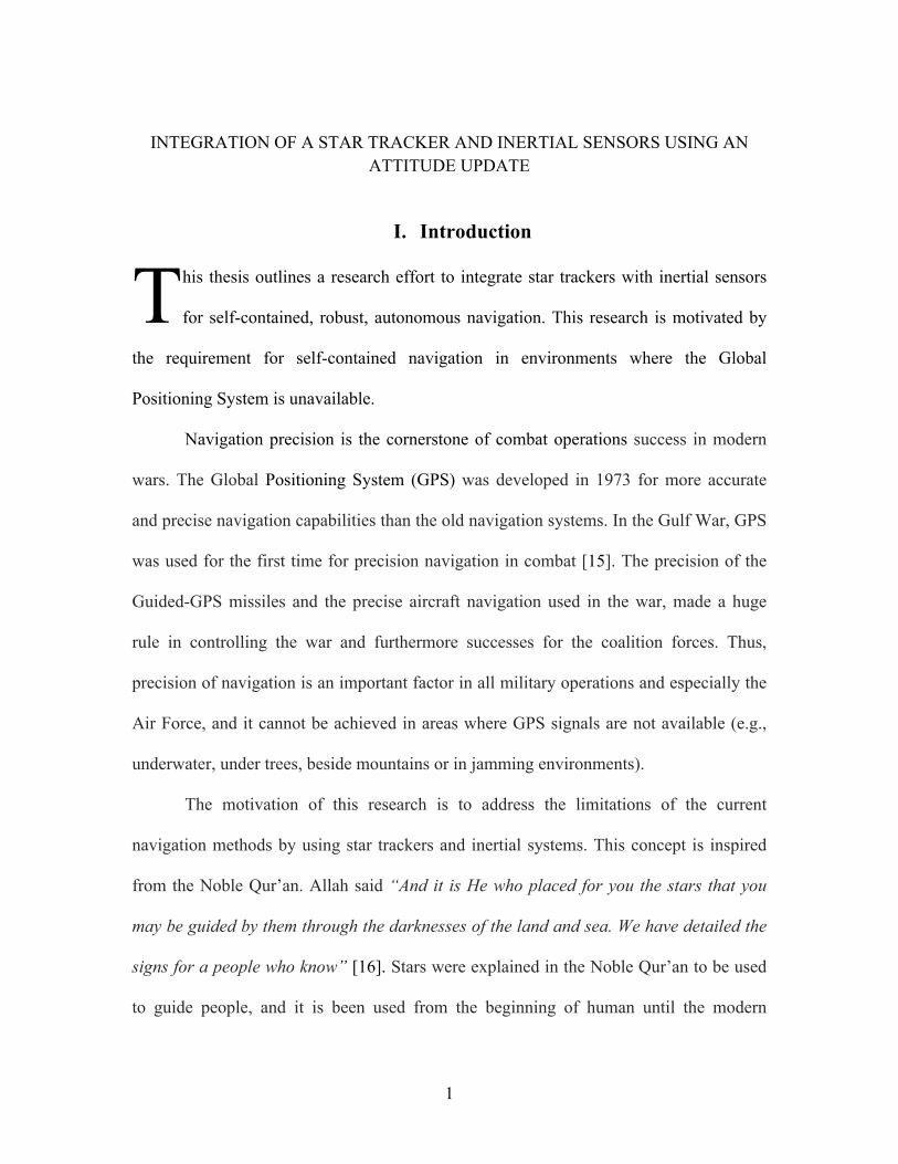
his thesis outlines a research effort to integrate star trackers with inertial sensors

for self-contained, robust, autonomous navigation. This research is motivated by

the requirement for self-contained navigation in environments where the Global

Positioning System is unavailable.

Navigation precision is the cornerstone of combat operations success in modern

wars. The Global Positioning System (GPS) was developed in 1973 for more accurate

and precise navigation capabilities than the old navigation systems. In the Gulf War, GPS

was used for the first time for precision navigation in combat [15]. The precision of the

Guided-GPS missiles and the precise aircraft navigation used in the war, made a huge

rule in controlling the war and furthermore successes for the coalition forces. Thus,

precision of navigation is an important factor in all military operations and especially the

Air Force, and it cannot be achieved in areas where GPS signals are not available (e.g.,

underwater, under trees, beside mountains or in jamming environments).

The motivation of this research is to address the limitations of the current

navigation methods by using star trackers and inertial systems. This concept is inspired

from the Noble Qur’an. Allah said “And it is He who placed for you the stars that you

may be guided by them through the darknesses of the land and sea. We have detailed the

signs for a people who know” [16]. Stars were explained in the Noble Qur’an to be used

to guide people, and it is been used from the beginning of human until the modern

T

2

century. With the new technology and the development of electronics, star trackers can

be advanced and enhanced with new navigation methods to be used with the inertial

sensors for precise navigation.

The following sections will explain the problem definition of the research, the

contributions to the research area, and the outline of the research chapters.

1.1 Problem Definition

Considering the unreliability of GPS, as it can be denied through external

interference, it is important to consider different navigation systems. An inertial

navigation system (INS) combined with a Celestial Navigation System (CNS) can

enhance the accuracy of navigating, by using star trackers mounted on the aircraft to

correct the accumulated errors in the INS.

Celestial navigation system primary consists of a star tracker mounted on a

navigating vehicle (e.g. aircraft, spacecraft, ship, and missile) that capture stars available

in the field of view of the star tracker camera and then compare it with a star catalogue

saved in the vehicle computer. From this process, the vehicle’s attitude can be estimated

and then used to aid the INS as an attitude update.

This research will simulate the star trackers when integrated with different

qualities of INS, and show the impact and improvement to the navigating vehicle.

3

1.2 Research Contributions

As mentioned in the previous section, the objective of this research is to simulate

and show the advantage of star trackers when used to aid different grades of the INS.

There are three primary contributions in the research. The first contribution is to

model the different grades of the INS (i.e. commercial, tactical, and navigation), and that

is described in Chapter III, Section 3.2.

The second contribution is to model different aiding measurements, which will be

the star tracker model, GPS, and barometer. The GPS model will be shown and explained

in Chapter III, Section 3.4.1. The barometer model will be explained in Chapter III,

Section 3.4.2. Finally, the star tracker model will be explained in Chapter III, Section

3.4.3.

The third contribution is to simulate the previous models in MATLAB, using

Kalman filter as an estimator, to show the performance development to the different

grades of INS.

1.3 Thesis Outline

This research is organized as follows. Chapter II will provides a mathematical

background for reference frames, transformation between reference frames, star tracker

concepts and specifications, linear and nonlinear Kalman filter estimators, and previous

work in the field of celestial navigation. Chapter III will presents the methodology used

in the research and the models developed. Chapter IV will show the simulation results of

the developed methodology and the impact of star tracker accuracy on the different

4

grades of INS. Finally, Chapter V will conclude the research results and provide

recommendations for future work related to the research.

5

II. Mathematical Background

his chapter reviews the mathematical background materials that are required to

understand the methodology used to aid the inertial navigation system using

celestial observations. The chapter begins with introduction to the inertial navigation

system. Next, the reference frames used in navigation are defined and the transformation

of coordinates between reference frames is explained. Then, the WGS-84 coordinate

system is reviewed. Next, star trackers are introduced along with their specifications. In

addition, a discussion of the Kalman filter is presented as a widely used recursive

estimation system. Finally, previous work related to this research is discussed.

2.1 Inertial Navigation System

The Inertial Navigation System (INS) is a navigation system that uses two types

of sensors and a processing computer to calculate the position, velocity and attitude of a

vehicle. There are two types of sensors used, accelerometers and gyroscopes [2]. An

accelerometer is a motion sensor that measures the specific force of a vehicle, and the

gyroscope is a rotation sensor that measures the angular velocity of a vehicle [2].

There are two types of INS, gimbaled and strapdown, and the Strapdown Inertial

Navigation System (SINS) will be used in the research. In the strapdown inertial

navigation system, the accelerometers and gyroscopes are directly mounted on the

vehicle body [2]. A diagram that explains the mechanism of the SINS is shown in Fig.

2.1.

T

6

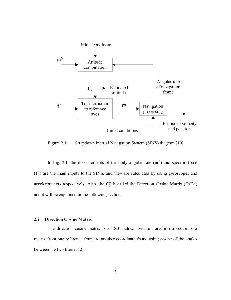
Figure 2.1: Strapdown Inertial Navigation System (SINS) diagram [10]

In Fig. 2.1, the measurements of the body angular rate (𝛚!) and specific force

(𝐟!) are the main inputs to the SINS, and they are calculated by using gyroscopes and

accelerometers respectively. Also, the 𝐂!! is called the Direction Cosine Matrix (DCM)

and it will be explained in the following section.

2.2 Direction Cosine Matrix

The direction cosine matrix is a 3×3 matrix, used to transform a vector or a

matrix from one reference frame to another coordinate frame using cosine of the angles

between the two frames [2].

Attitude computation

Transformation to reference

axes

Navigation processing

Estimated attitude

Angular rate of navigation

frame

Initial conditions

Estimated velocity and position Initial conditions

𝐟! 𝐟!

𝛚!

𝐂!!

7

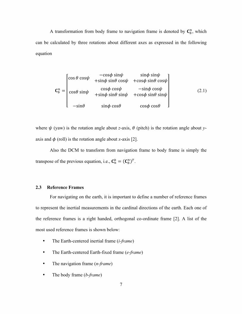
A transformation from body frame to navigation frame is denoted by 𝐂!!, which

can be calculated by three rotations about different axes as expressed in the following

equation

𝐂!! =

cos𝜃 cos𝜓 −cos𝜙 sin𝜓+sin𝜙 sin𝜃 cos𝜓

sin𝜙 sin𝜓+cos𝜙 sin𝜃 cos𝜓

cos𝜃 sin𝜓 cos𝜙 cos𝜓+sin𝜙 sin𝜃 sin𝜓

−sin𝜙 cos𝜓+cos𝜙 sin𝜃 sin𝜓

−sin𝜃 sin𝜙 cos𝜃 cos𝜙 cos𝜃

(2.1)

where 𝜓 (yaw) is the rotation angle about z-axis, 𝜃 (pitch) is the rotation angle about y-

axis and 𝜙 (roll) is the rotation angle about x-axis [2].

Also the DCM to transform from navigation frame to body frame is simply the

transpose of the previous equation, i.e., 𝐂!! = 𝐂!! !.

2.3 Reference Frames

For navigating on the earth, it is important to define a number of reference frames

to represent the inertial measurements in the cardinal directions of the earth. Each one of

the reference frames is a right handed, orthogonal co-ordinate frame [2]. A list of the

most used reference frames is shown below:

• The Earth-centered inertial frame (i-frame)

• The Earth-centered Earth-fixed frame (e-frame)

• The navigation frame (n-frame)

• The body frame (b-frame)

8

• The sensor frame (s-frame)

Each of the frames is described in the following subsections.

2.3.1 Earth-Centered Inertial Frame (i-frame)

The Earth-centered inertial frame has its origin at the center of the earth and its

axes (𝑥! ,𝑦! and 𝑧!) are non-rotating with respect to the fixed stars [2], see Fig. 2.2 for

axes illustration.

2.3.2 Earth-Centered Earth-Fixed Frame (e-frame)

The Earth-centered Earth-fixed frame has its origin at the center of the earth and

its axes are fixed with respect to the earth. Its axes are defined by 𝑥! ,𝑦! and 𝑧!. The 𝑥!

axis lies along the intersection of the plane of the Greenwich meridian and the earth’s

equatorial plane, the 𝑧! axis is aligned with the North Pole and the 𝑦! axis is

perpendicular to 𝑥!and 𝑧! with a direction that follows the right hand rule. The Earth-

centered Earth-fixed frame rotates with respect to the inertial frame, at a rate of 𝜔!" about

the 𝑧! axis [2]. See Fig. 2.2 which includes an illustration of the e-frame axes.

2.3.3 Navigation Frame (n-frame)

The navigation frame is denoted by n and has its origin at the location of the

navigation system. Its axes are aligned with the directions of north, east, and local

vertical (down), defined by 𝑥! ,𝑦! and 𝑧! respectively in Fig. 2.2. The turn rate of the

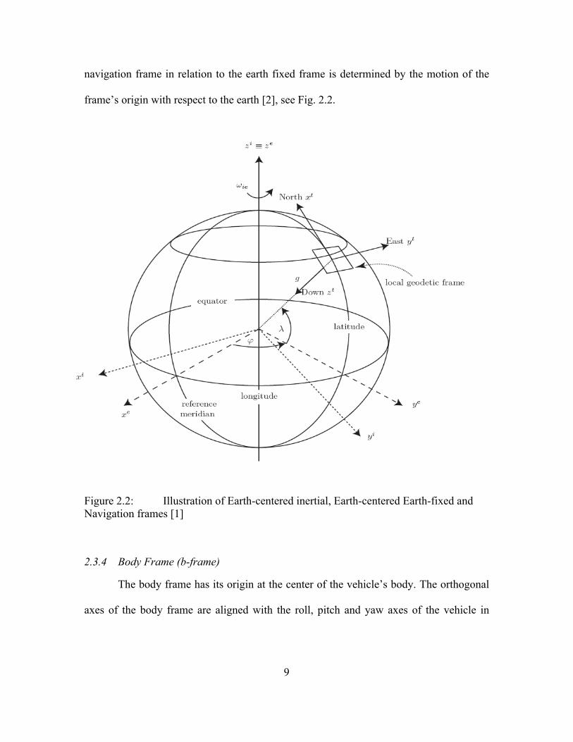
9

navigation frame in relation to the earth fixed frame is determined by the motion of the

frame’s origin with respect to the earth [2], see Fig. 2.2.

Figure 2.2: Illustration of Earth-centered inertial, Earth-centered Earth-fixed and Navigation frames [1]

2.3.4 Body Frame (b-frame)

The body frame has its origin at the center of the vehicle’s body. The orthogonal

axes of the body frame are aligned with the roll, pitch and yaw axes of the vehicle in

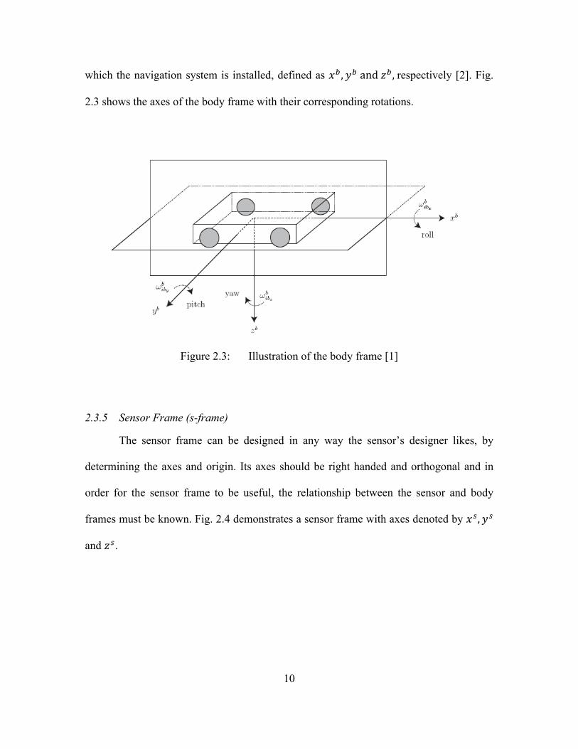
10

which the navigation system is installed, defined as 𝑥! ,𝑦! and 𝑧! , respectively [2]. Fig.

2.3 shows the axes of the body frame with their corresponding rotations.

Figure 2.3: Illustration of the body frame [1]

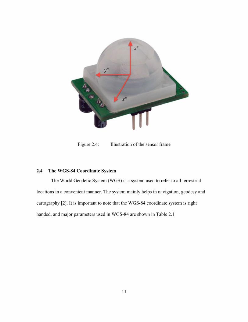
2.3.5 Sensor Frame (s-frame)

The sensor frame can be designed in any way the sensor’s designer likes, by

determining the axes and origin. Its axes should be right handed and orthogonal and in

order for the sensor frame to be useful, the relationship between the sensor and body

frames must be known. Fig. 2.4 demonstrates a sensor frame with axes denoted by 𝑥!,𝑦!

and 𝑧!.

11

Figure 2.4: Illustration of the sensor frame

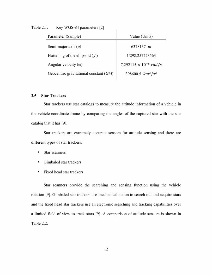
2.4 The WGS-84 Coordinate System

The World Geodetic System (WGS) is a system used to refer to all terrestrial

locations in a convenient manner. The system mainly helps in navigation, geodesy and

cartography [2]. It is important to note that the WGS-84 coordinate system is right

handed, and major parameters used in WGS-84 are shown in Table 2.1

𝑥!

𝑦!

𝑧!

12

Table 2.1: Key WGS-84 parameters [2]

Parameter (Sample) Value (Units)

Semi-major axis (a)

Flattening of the ellipsoid ( f )

Angular velocity (ω)

Geocentric gravitational constant (GM)

6378137 𝑚

1/298.257223563

7.292115 × 10!! 𝑟𝑎𝑑/𝑠

398600.5 𝑘𝑚!/𝑠!

2.5 Star Trackers

Star trackers use star catalogs to measure the attitude information of a vehicle in

the vehicle coordinate frame by comparing the angles of the captured star with the star

catalog that it has [9].

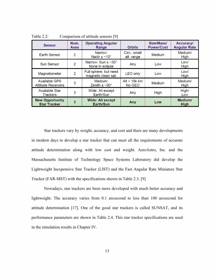
Star trackers are extremely accurate sensors for attitude sensing and there are

different types of star trackers:

• Star scanners

• Gimbaled star trackers

• Fixed head star trackers

Star scanners provide the searching and sensing function using the vehicle

rotation [9]. Gimbaled star trackers use mechanical action to search out and acquire stars

and the fixed head star trackers use an electronic searching and tracking capabilities over

a limited field of view to track stars [9]. A comparison of attitude sensors is shown in

Table 2.2.

13

Table 2.2: Comparison of attitude sensors [9]

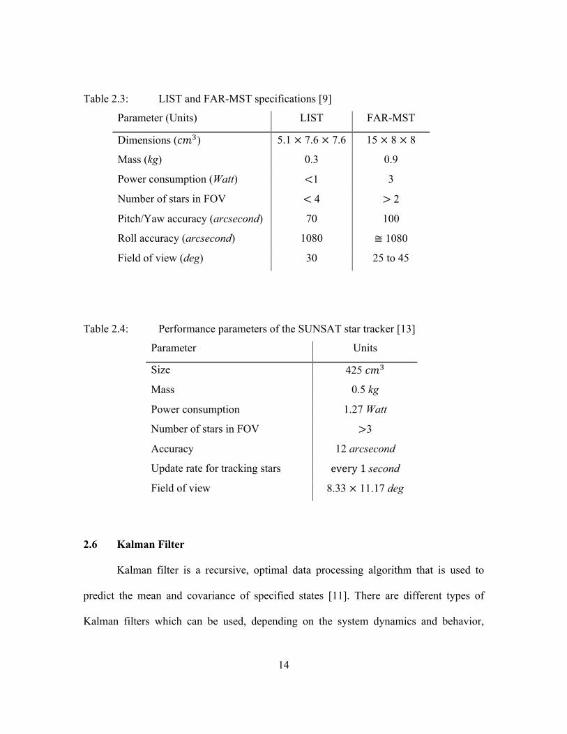
Star trackers vary by weight, accuracy, and cost and there are many developments

in modern days to develop a star tracker that can meet all the requirements of accurate

attitude determination along with low cost and weight. AeroAstro, Inc. and the

Massachusetts Institute of Technology Space Systems Laboratory did develop the

Lightweight Inexpensive Star Tracker (LIST) and the Fast Angular Rate Miniature Star

Tracker (FAR-MST) with the specifications shown in Table 2.3. [9]

Nowadays, star trackers are been more developed with much better accuracy and

lightweight. The accuracy varies from 0.1 arcsecond to less than 100 arcsecond for

attitude determination [17]. One of the good star trackers is called SUNSAT, and its

performance parameters are shown in Table 2.4. This star tracker specifications are used

in the simulation results in Chapter IV.

Chapter 1 – Background and Motivation for Work 35

As evident in these examples, star trackers have been implemented onboard some of the

most sophisticated aircraft, spacecraft, and satellites that have accomplished impressive feats.

Star trackers were selected as the primary attitude sensors in these missions because of their

potential for high sensing and tracking accuracy. The unfortunate tradeoff for high precision is

significant increases in mass, computational expense, and power consumption. Regardless, all of

these missions were multi-million dollar ventures where the most advanced attitude sensors were

not only appropriate, but were crucial, and so these tradeoffs were relatively inconsequential.

However, there are numerous current missions, many of which have a high potential for

significant scientific advancement, that cannot afford the large increases in mass, computational

expense or power consumption. Whether these missions emanate from small start-up companies

or large government proposals, their objectives remain high. The pervasive requirement to drive

down overall weight and volume of satellites and spacecraft in order to minimize propulsive

expenses for launch will require attitude sensors that are small enough to accompany their

reduced hardware sizes, while simultaneously maintaining their effectiveness in attitude

determination. The second through fifth rows of Table 1.2 describe the five attitude sensors

discussed above. It is clear from this table that current star trackers can perform under the most

variable operating conditions and can provide the most accurate attitude information, but these

advantages come at the expense of requiring the greatest size, mass, power consumption, and

cost.

Table 1.2 Comparison of Current Attitude Sensors

14

Table 2.3: LIST and FAR-MST specifications [9]

Parameter (Units) LIST FAR-MST

Dimensions (𝑐𝑚!) 5.1 × 7.6 × 7.6 15 × 8 × 8

Mass (kg) 0.3 0.9

Power consumption (Watt) <1 3

Number of stars in FOV < 4 > 2

Pitch/Yaw accuracy (arcsecond) 70 100

Roll accuracy (arcsecond) 1080 ≅ 1080

Field of view (deg) 30 25 to 45

Table 2.4: Performance parameters of the SUNSAT star tracker [13]

Parameter Units

Size 425 𝑐𝑚!

Mass 0.5 kg

Power consumption 1.27 Watt

Number of stars in FOV >3

Accuracy 12 arcsecond

Update rate for tracking stars every 1 second

Field of view 8.33 × 11.17 deg

2.6 Kalman Filter

Kalman filter is a recursive, optimal data processing algorithm that is used to

predict the mean and covariance of specified states [11]. There are different types of

Kalman filters which can be used, depending on the system dynamics and behavior,

15

including linear and nonlinear Kalman filters. For the nonlinear Kalman filter, there are

two famous systems used for nonlinear systems, the Unscented Kalman Filter (UKF) and

the Extended Kalman Filter (EKF). This research will focus on the linear Kalman filter

and could use aspects of the unscented Kalman filter.

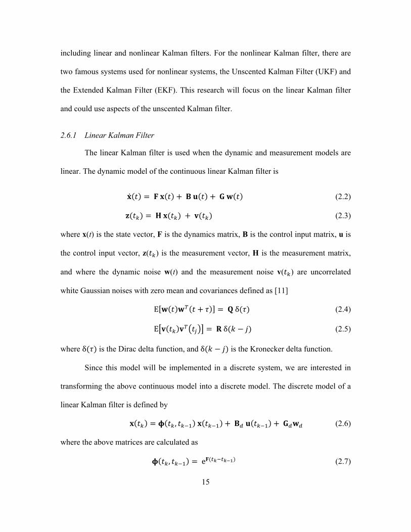
2.6.1 Linear Kalman Filter

The linear Kalman filter is used when the dynamic and measurement models are

linear. The dynamic model of the continuous linear Kalman filter is

𝐱 𝑡 = 𝐅 𝐱 𝑡 + 𝐁 𝐮 𝑡 + 𝐆 𝐰 𝑡 (2.2)

𝐳(𝑡!) = 𝐇 𝐱(𝑡!) + 𝐯(𝑡!) (2.3)

where x(t) is the state vector, F is the dynamics matrix, B is the control input matrix, u is

the control input vector, z(𝑡!) is the measurement vector, H is the measurement matrix,

and where the dynamic noise w(t) and the measurement noise v(𝑡!) are uncorrelated

white Gaussian noises with zero mean and covariances defined as [11]

E 𝐰 𝑡 𝐰! 𝑡 + 𝜏 = 𝐐 δ(𝜏) (2.4)

E 𝐯 𝑡! 𝐯! 𝑡! = 𝐑 δ(𝑘 − 𝑗) (2.5)

where δ(𝜏) is the Dirac delta function, and δ(𝑘 − 𝑗) is the Kronecker delta function.

Since this model will be implemented in a discrete system, we are interested in

transforming the above continuous model into a discrete model. The discrete model of a

linear Kalman filter is defined by

𝐱 𝑡! = 𝛟 𝑡! , 𝑡!!! 𝐱 𝑡!!! + 𝐁! 𝐮 𝑡!!! + 𝐆!𝐰! (2.6)

where the above matrices are calculated as

𝛟 𝑡! , 𝑡!!! = e𝐅(!!!!!!!) (2.7)

16

𝐁! = 𝐅!!(𝛟 𝑡! , 𝑡!!! − 𝐈)𝐁 (2.8)

𝐆! = 𝐈 (2.9)

And 𝐰! is a zero mean white Gaussian noise with covariance defined by

𝐐! = E[w!w!!] (2.10)

where 𝐐! can be found by using the Van Loan Method to convert from continuous to

discrete noise [11].

Kalman filtering consists of two steps, time propagation and measurement

updates. The quantities that we are interested in are the mean and covariance of the states,

which will be given the symbols 𝐱! and 𝐏!, respectively.

2.6.1.1 Propagation Propagation consists of estimating the current mean

and covariance using the previous mean and covariance [11], we define propagation as

𝐱!!! = 𝛟 𝑡! , 𝑡!!! 𝐱!!!!

! + 𝐁!u!!!! (2.11)

𝐏!!! = 𝛟 𝑡! , 𝑡!!! P!!!!

! 𝛟𝑻 𝑡! , 𝑡!!! + 𝐐! (2.12)

where "-" denotes the previous value before the measurement update and "+" denotes the

value after the measurement update.

2.6.1.2 Measurement Update When a measurement z! is available at time

k, the states are updated in the following manner

𝐱!!! = 𝐱!!

! + 𝐊!! 𝐳!! − 𝐇!!𝐱!!! (2.13)

where 𝐊! is the kalman filter gain, and it is given by the following equation

𝐊!! = (𝐇!!𝐏!!! )! [𝐇!!𝐏!!

!𝐇!!! + 𝐑!!]

!! (2.14)

17

And 𝐇! is the measurement matrix. Using the gain and measurement matrix, the

covariance after an update can be calculated by

𝐏!!! = 𝐈− 𝐊!!𝐇!! 𝐏!!

! (2.15)

2.6.2 Unscented Kalman Filter

The Unscented Kalman Filter (UKF) is used for nonlinear systems and it is based

on the principle of using a set of appropriately chosen weighted points to parameterize

the means and covariances of probability distributions [6]. The UKF is based on the

unscented transformation, which is the transformation of a set of so-called sigma points,

using a nonlinear function [6]. The sigma points along with their weighting are chosen in

a well-known algorithm, which is given by the following equations:

𝜒! = 𝑥 𝑊! =!

!!! (2.16)

𝜒! = 𝑥 + 𝑛 + 𝑘 𝑃!! ! 𝑊! =

!! !!!

(2.17)

𝜒!!! = 𝑥 − 𝑛 + 𝑘 𝑃!! ! 𝑊!!! =

!! !!!

(2.18)

where 𝜒 denotes the sigma points, and 𝑊 is the associated weight of the sigma points.

These sigma points are passed through a nonlinear mapping function to result in

transformed sigma points [6]. The transformed sigma points with their mean and

covariance are shown by the following equations:

The transformed sigma points are

𝒴! = 𝑓 [𝜒!] (2.19)

The weighted mean of the transformed sigma points is

18

𝑦 = 𝑊! 𝒴!!!!!! (2.20)

The weighted covariance of the transformed sigma points is

𝑃!! = 𝑊! {𝒴! − 𝑦}!!!!! {𝒴! − 𝑦}! (2.21)

The UKF performs exactly like the Second Order Gauss Filter but without the

need to calculate Jacobeans of the nonlinear functions in the system [6]. The ease of

implementation and the high estimation accuracy of the unscented transformation (UKF),

sometimes make it better filtering/estimation algorithm than the Extended Kalman Filter

(EKF) for nonlinear systems [6].

2.7 Previous Work

In this section, previous work related to my thesis will be presented and discussed.

It will include researches in the celestial navigation field.

2.7.1 Correction Technique for Velocity and Position Errors of Inertial Navigation

System by Celestial Observations [3]

Gul and Jiancheng [3] presented a technique to correct some of the accumulated

errors in the inertial navigation system (INS) of a space vehicle using stars observations.

The accumulated errors that were considered in their research are:

• Accelerometer bias.

• Gyro drift (𝜀).

• Initial misalignment error (𝜑!).

In their research, a ballistic missile is simulated to demonstrate the validity of the

method. The flight path of the missile is divided into three phases. The first phase is from

19

the launch point until the missile crosses the atmosphere, the second phase is from the

point where the missile crosses the atmosphere to the point of burnout (the point where

the engine of the missile is disconnected), and the third phase is after the burnout point to

the point of impact of the missile with the ground target.

The misalignment error (𝜑!") is calculated by observing a star at time 𝑡𝑚 after

the missile crosses the atmosphere, using a star tracker mounted on the missile, then a

few seconds later another star observation is made which results in a second

misalignment error (𝜑!"!!) at time 𝑡𝑚 + 𝜏. Using the two calculated observations, the

gyro drift (ε) can be calculated as follows:

𝜑!"!! − 𝜑!" = 𝐂!!!"!!!" 𝑑𝑡 𝜀 = 𝐏 𝜀 (2.22)

𝜀 = 𝐏!!(𝜑!"!! − 𝜑!") (2.23)

where 𝐂!! is the DCM to transform from the body frame to the inertial frame.

Using the gyro drift in (2.23), the initial misalignment error (𝜑!) is calculated by

𝜑! = 𝜑!" − 𝑡𝑚 𝜀 (2.24)

By using the gyro drift and the initial misalignment error, the position and

velocity of the missile is corrected at this time. After the burnout point, the missile takes

in a free flight motion until it hits the ground target, so the output of the accelerometer of

the missile’s INS after the burnout point is used as the accelerometer bias. Then, the

position and velocity errors due to the accelerometer bias can be calculated to correct the

position and velocity of the missile.

The celestial navigation method used in the research [3] is simulated for 200

seconds flight time for a ballistic missile, providing a tremendous enhancement for the

20

INS of the missile. The technique presented in the research is valid for small

misalignment angles and gyro drift. The technique could be enhanced to result in more

accurate results by using Kalman filters to reduce the propagated errors in the INS.

However, their technique does not apply for aircraft trajectories, because there is not a

free-fall portion of the trajectory.

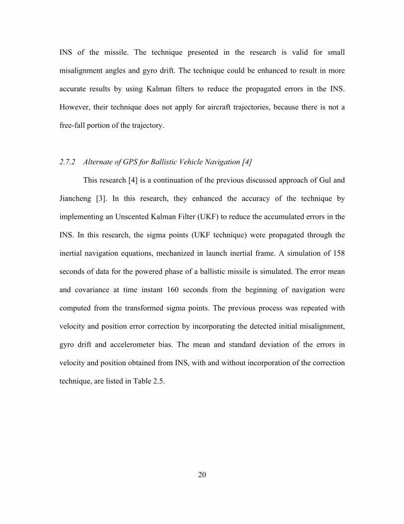
2.7.2 Alternate of GPS for Ballistic Vehicle Navigation [4]

This research [4] is a continuation of the previous discussed approach of Gul and

Jiancheng [3]. In this research, they enhanced the accuracy of the technique by

implementing an Unscented Kalman Filter (UKF) to reduce the accumulated errors in the

INS. In this research, the sigma points (UKF technique) were propagated through the

inertial navigation equations, mechanized in launch inertial frame. A simulation of 158

seconds of data for the powered phase of a ballistic missile is simulated. The error mean

and covariance at time instant 160 seconds from the beginning of navigation were

computed from the transformed sigma points. The previous process was repeated with

velocity and position error correction by incorporating the detected initial misalignment,

gyro drift and accelerometer bias. The mean and standard deviation of the errors in

velocity and position obtained from INS, with and without incorporation of the correction

technique, are listed in Table 2.5.

21

Table 2.5: Error statistics at time instant 160 seconds from launch time [4]

Parameter

(Units)

Without correction With correction

Mean 1-sigma Mean 1-sigma

V! (m/s) -0.019 8.494 0.004 0.013

V! (m/s) -0.009 6.932 0 0.014

V! (m/s) 0 10.910 0.006 0.012

r! (m) -1.51 739.60 0.01 1.23

r! (m) -0.91 476.70 0.62 1.98

r! (m) 0 878.15 0.17 0.79

In Table 2.5, V!, V!, V!, r!, r! and r! are the missile velocity and position in three

axes, respectively. From table 1, the results show that the velocity errors (1-sigma) are

reduced from (7 to 11) m/s to less than 0.015 m/s along each axis. Also, position errors

(1-sigma) are reduced from (470 to 870) meters to less than 2 meters along each axis.

The results found by using the UKF gives a motivation for further analysis by

implementing different types of Kalman filters.

2.7.3 Compass Star Tracker for GPS-like Applications [7]

Samaan, Mortari and Juan in their article [7] have made an in depth description

and analysis of the Compass Star Tracker, which is believed to be a new technological

innovation with regards to estimating of attitude and location of spacecrafts. The article

outlines the alignment of camera optical axis in relation to the gravitational direction and

time as the basic concept behind this system. Although the system employees the use of a

22

number of significant concepts of Global Positioning System (GPS), it cannot be used as

its substitute due to the fact that it suffers from the night-only limitation in addition to the

need for calm and clear weather conditions [7].

The Compass Star Tracker (CST) application can be applied when navigating in

non-GPS environments such as the Moon and planets or as backup system when GPS

fails, with its accuracy depending on aspects such as CCD resolution, time precision and

centroiding accuracy [7]. In this article, they described the estimation of latitude and

longitude positions in space using the Monte-Carlo stimulated image and the night sky

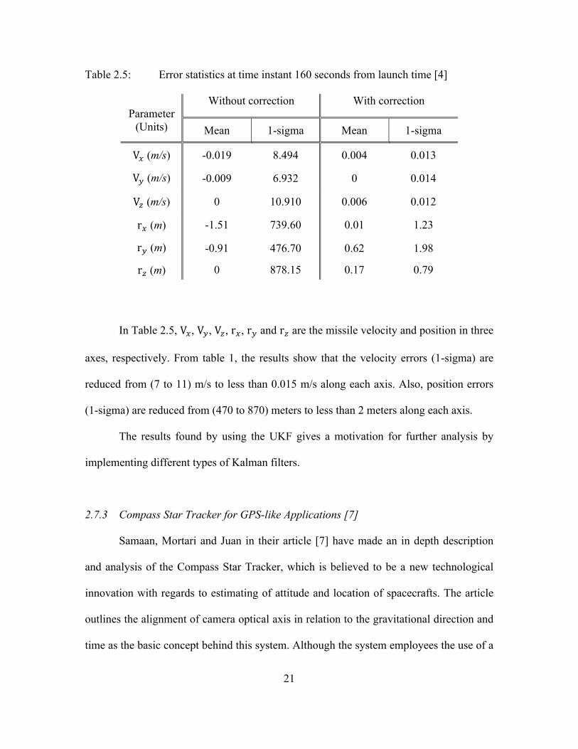
test through a gravity pendulum [7]. Their description embraces the use of the earth

centered inertial frame and camera body frame (axes x, y, z) as shown in Fig. 2.5.

Figure 2.5: Reference frame for Earth and optical axis [7]

to determine longitude and latitude of the currentlocation where the star image is taken. In order togive a correct output, the only condition required isthat the optical axis of the star sensor is aligned withrespect to the local effective gravity field vector. Whenthis occurs, then the picture contains all the neededinformation. The night sky image is then processed,and the star centroiding and star identificationprocesses then allow the evaluation of the star trackerattitude with respect to the inertial frame. By knowingthe current time of the captured star image, thelongitude and latitude of the current position will bedetermined using some simple attitude transformationsand the knowledge of time. Knowledge of the Earth’sgravity model enables us to establish the latitudeconsistent with the star image. A primary limitationis the precision of the alignment of the tracker axiswith the local gravity (plumb-bob) direction.This paper describes the technique developed

to estimate latitude and longitude of the observingposition and validate it by means of Monte-Carlosimulated images. Also, real night sky tests using astar camera and a gravity pendulum, a weight on theend of a rigid rod, have been accomplished to validatethis idea.There are many applications for this instrument.

One could be to use it for navigation in a non-GPSenvironment (e.g., Moon, Mars or the other planets,etc) or as a back-up in the case of GPS failure. Ofcourse the accuracy of this compass will depend onmany factors which include: 1) the CCD resolution, 2)the centroiding accuracy, 3) the time precision, and 4)the deviation between the local vertical alignment ofthe tracker with respect to the direction of gravity. Thelatter is caused mostly by the deviation of the actualEarth with the adopted Earth model (sphere, ellipsoid,geoid).

PROBLEM FORMULATION

In order to define the problem of the compass startracker, consider the Earth Centered Inertial (ECI)reference frame along with the camera body frame(axes [x,y,z]) as shown in Fig. 1. In this figure, thecamera optical axis (OA´ x) is assumed to be alignedwith the local vertical. To start, let us consider theEarth shape to be spherical. The theory associatedwith ellipsoidal or more accurate description of theEarth, will be treated later. The parameters appearingin Fig. 1 have the following meaning

1) ¸ and ' are the geographical longitude andlatitude.2) Ã is the angle between Vernal equinox (°) and

Greenwich meridian (G). This angle depends on thetime only.3) " is the angle between the local East (E) and

the y-axis of the camera body frame, and

Fig. 1. Reference frame for Earth and optical axis.

Let AB=I be the attitude matrix for the camera bodyframe with respect to ECI and AB=L the attitude matrixfor the camera body frame with respect to the localreference frame. We can write (Cx ´ cosx, Sx ´ sinx)

AB=L ´ R3(") =

2

64C" S" 0

¡S" C" 0

0 0 1

3

75 : (1)

Also, if AL=G is the attitude matrix for the localreference frame with respect to the Greenwichreference frame, then

AL=G ´ R2(¡')R3(¸)

=

2

64C' 0 S'

0 1 0

¡S' 0 C'

3

75

2

64Ç S¸ 0

¡S¸ Ç 0

0 0 1

3

75

=

2

64C'Ç C'S¸ S'

¡S¸ Ç 0

¡S'Ç ¡S'S¸ C'

3

75 : (2)

Let AG=I(t) be the Earth attitude matrix with respectto J2000, a matrix that is a function of the currenttime only. This matrix can also take into account theprecession and nutation of the Earth spin axis [1] as

AG=I(t) = R3(Ã)M (3)

where M is the rotation matrix that accounts theprecession and the nutation of the Earth, as given inthe next section.The three unknown parameters of the CST are ¸,

', and ". These parameters could be solved using thefollowing identity

AB=I = AB=LAL=GAG=I: (4)

By using (1) and (2), we obtain the expression for thetransformation matrix AB=G = AB=LAL=G

AB=G =

2

64C"C'Ç¡ S"S¸ S"Ç+C"C'S¸ C"S'

¡S"C'Ç¡C"S¸ C"Ç¡ S"C'S¸ ¡S"S'¡S'Ç ¡S'S¸ C'

3

75 :

(5)

1630 IEEE TRANSACTIONS ON AEROSPACE AND ELECTRONIC SYSTEMS VOL. 44, NO. 4 OCTOBER 2008

23

In Fig. 2.5, the x-axis is the camera optical axis, aligned to the local vertical.

There are number of parameters in the figure, defined as, λ being the longitude, φ the

latitude, ψ the angle between the vernal equinox (𝛾) and the Greenwich Meridian (G),

and ԑ is the angle between the camera’s y-axis and the local East (E). Samaan, Mortari

and Juan identified these as the unknown parameters that to be calculated.

In the following equations, there are reference frames that to be explained. The

subscript B is used for the body frame of the camera, G as the Greenwich frame, I as the

inertial frame and L as the local frame [7].

Assume AB/I is the attitude matrix for the camera body frame with respect to the

inertial frame and assume that AB/L is the attitude matrix for the camera body frame with

respect to the local frame [7], then

AB/L ≡ R3 (ε) =cos 𝜀 sin 𝜀 0− sin 𝜀 cos 𝜀 00 0 1

(2.25)

Also, assume that AL/G is the attitude matrix for the local reference frame

with respect to the Greenwich frame [7], then

AL/G ≡ R2 (-φ) R3 (λ) (2.26)

AL/G =cos𝜑 0 sin𝜑0 1 0

− sin𝜑 0 cos𝜑 cos 𝜆 sin 𝜆 0− sin 𝜆 cos 𝜆 00 0 1

(2.27)

These equations relate through the equation AB/G = AB/I AI/G = AB/L AL/G = AB/G ,

that can be used to solve the unknown parameters using the following equations

The latitude φ is computed by

𝐶! = A!! 3,3 (2.28)

24

The longitude 𝜆 is computed by

tan 𝜆 = !!!/! (!,!)

!!!/! (!,!) (2.29)

The East direction ԑ is computed by

tan 𝜀 = !!!/! (!,!)

!!/! (!,!) (2.30)

Using the night sky test that employed the use of a star image captured by a

Star1000 camera, Samaan, Mortari and Juan carried out a centroiding algorithm to find

the star centers, while star identification was done using the Pyramid Star-ID technique.

This led to estimating the attitude matrix AB/I using the ESOQ-2 algorithm. Having been

able to find the time of the measured image, the AG/I matrix was evaluated [7].

Consequently, the equation matrixes, led to identifying the longitude and latitude,

with 0.0080 and 0.020 errors, respectively, as compared to the actual longitude and

latitude values of a GPS receiver [7]. The Monte-Carlo simulation was also applied

through the use of a camera with its optical axis pointing at the zenith. They selected the

longitude to be at – 104.96580 and the latitude at 39.75460 with a compass angle ԑ of 100.

After obtaining the initial and observed directions of the star, an optimal estimate of

attitude matrix is done using the ESOQ-2 estimator, and the estimated values of the

longitude was found to be –104.97040, latitude of 39.75280 and local east angle of

10.03930 [7].

For Samaan, Mortari and Juan, these results provided optimism in the CST

approach through which standard algorithm can be used in processing the images of stars

25

and location of the stars using a camera [7]. Although this method seems applicable, it

has limitations of accuracy in the system, which necessitates more research and studies

through which WGS-84 model would be quantified. Samaan, Mortari and Juan have

evidently brought into light the possibility of using star trackers in estimating position

together with attitude [7].

2.8 Chapter Summary

In this chapter, mathematical background related to the research was discussed

and explained. In the next chapter, the methodology that will be used in the research will

be explained in details.

26

III. Methodology

his chapter will explain the mathematical approach for simulating the inertial

navigation system aided by a star tracker, global positioning system, and

barometer. The chapter is organized as follows. First, a block diagram that describes the

system structure is shown. Second, a truth model that represents the true trajectory of the

aircraft will be presented. Next, a dynamic model for the inertial navigation system error

model is explained in detail. Finally, measurements models for different measurements

sources are discussed and explained.

3.1 System Block Diagram

The system block diagram is important to understand the functions and rule of the

different components in the system. Fig. 3.1 shows the interrelationships between the

system’s components in a functional block diagram.

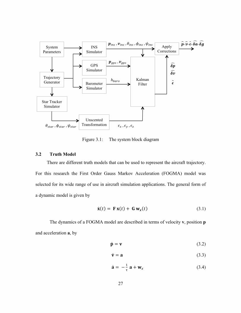
In the system block diagram, we first start to generate the system parameters that

will have all the parameters of the navigating vehicle. Then, we generate a truth trajectory

using Trajectory Generator block, which will be explained in the next Section. Next, we

use the INS simulator to generate the system dynamics, and it will be explained in

Section 3.3. The GPS, barometer, and star tracker measurements are generated by using

the truth trajectory plus additional sensors biases, the measurement models will be shown

and explained in Section 3.4. Then, a Kalman filter is used to estimate the navigation

errors. Finally, we use the estimated errors to correct the INS navigation parameters.

T

27

Figure 3.1: The system block diagram

3.2 Truth Model

There are different truth models that can be used to represent the aircraft trajectory.

For this research the First Order Gauss Markov Acceleration (FOGMA) model was

selected for its wide range of use in aircraft simulation applications. The general form of

a dynamic model is given by

𝐱 𝑡 = 𝐅 𝐱 𝑡 + 𝐆 𝐰𝒙 𝑡 (3.1)

The dynamics of a FOGMA model are described in terms of velocity v, position p

and acceleration a, by

𝐩 = 𝐯 (3.2)

𝐯 = 𝐚 (3.3)

𝐚 = − !! 𝐚+𝐰! (3.4)

!!"# !,!!"# !,!!"#!,!!"#!,!!"#

!!"#!,!!"#

!!"#$!,!!"#$ !,!!"#$ !! !, !!!, !!

!"! !

!"! !

!!

!!,!!, !!, !"! ,!"!

I. Methodology

his chapter will explain the mathematical approach for simulating the inertial

navigation system aided by a star tracker, global positioning system, and barometer.

The chapter is organized as follows. First, a block diagram that describes the system

structure is shown. Second, a truth model that represents the true trajectory of the aircraft

will be presented. Next, a dynamic model for the inertial navigation system error model is

explained in detail. Finally, measurements models for different measurements sources are

discussed and explained.

1.1 System block diagram

The system block diagram is important to understand the functions and rule of the

different components in the system. Figure 3.1 shows the interrelationships between the

system’s components in a functional block diagram.

Figure 3.1: The system block diagram

T

System Parameters

Trajectory Generator

GPS Simulator

INS Simulator

Barometer Simulator

Star Tracker Simulator

Kalman Filter

Unscented Transformation

ℎ!"#$

Apply Corrections

28

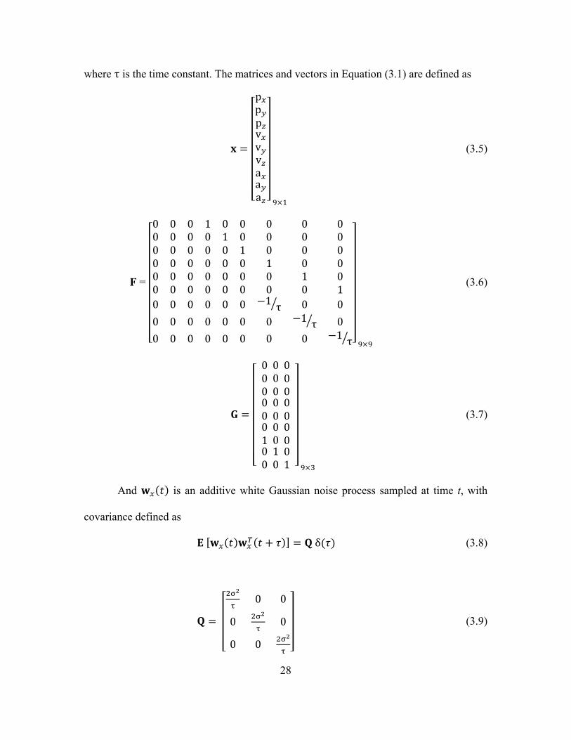
where τ is the time constant. The matrices and vectors in Equation (3.1) are defined as

𝐱 =

p!p!p!v!v!v!a!a!a! !×!

(3.5)

F =

0 0 0 1 0 0 0 0 00 0 0 0 1 0 0 0 00 0 0 0 0 1 0 0 00 0 0 0 0 0 1 0 00 0 0 0 0 0 0 1 00 0 0 0 0 0 0 0 10 0 0 0 0 0 −1 τ 0 00 0 0 0 0 0 0 −1 τ 00 0 0 0 0 0 0 0 −1 τ !×!

(3.6)

𝐆 =

0 0 0 0 0 0 1 0 0

0 0 0 0 0 0 0 1 0

0 0 0 0 0 0 0 0 1 !×!

(3.7)

And 𝐰! 𝑡 is an additive white Gaussian noise process sampled at time t, with

covariance defined as

𝐄 𝐰! 𝑡 𝐰!! 𝑡 + 𝜏 = 𝐐 δ(𝜏) (3.8)

𝐐 =

!!!

!0 0

0 !!!

!0

0 0 !!!

!

(3.9)

29

where σ! is the desired variance of the components of acceleration vector a!, a!, and a!,

and δ(𝜏) is the Dirac delta function.

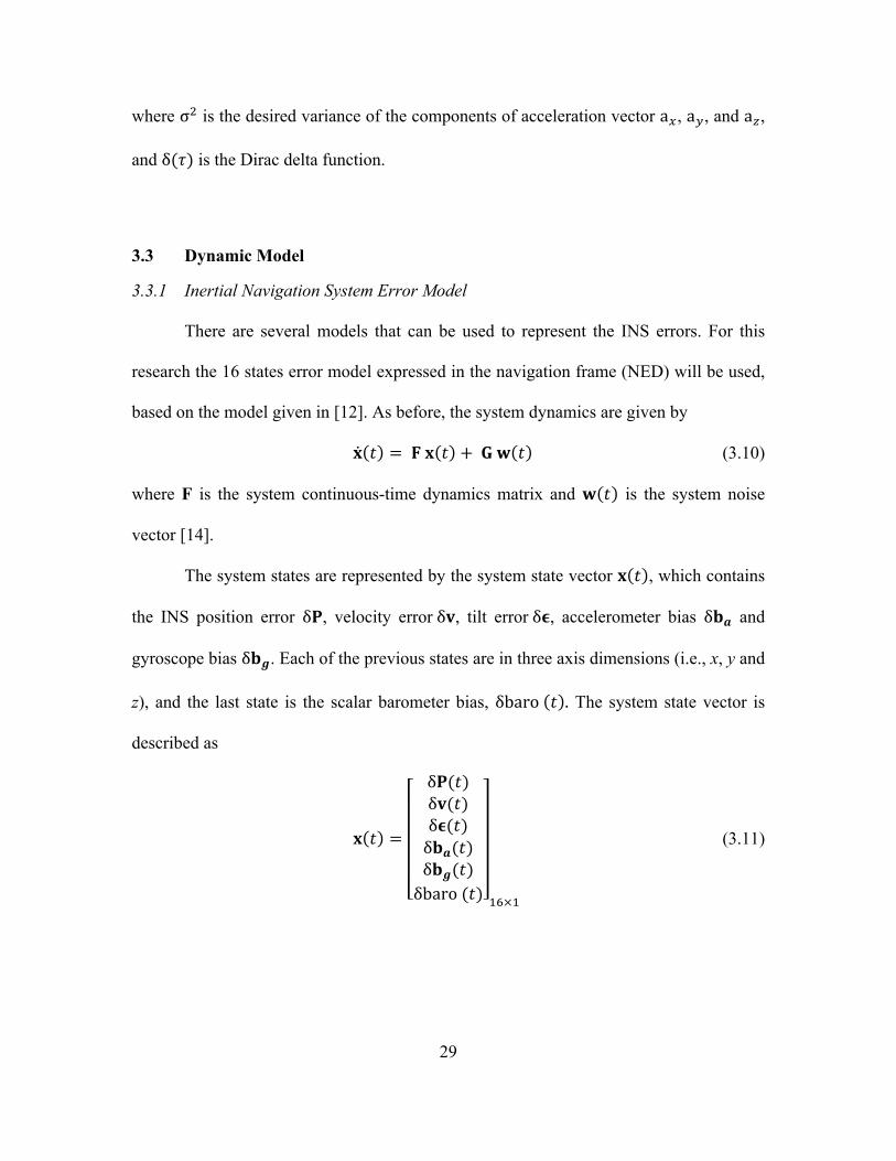
3.3 Dynamic Model

3.3.1 Inertial Navigation System Error Model

There are several models that can be used to represent the INS errors. For this

research the 16 states error model expressed in the navigation frame (NED) will be used,

based on the model given in [12]. As before, the system dynamics are given by

𝐱 𝑡 = 𝐅 𝐱 𝑡 + 𝐆 𝐰 𝑡 (3.10)

where F is the system continuous-time dynamics matrix and 𝐰 𝑡 is the system noise

vector [14].

The system states are represented by the system state vector 𝐱 𝑡 , which contains

the INS position error δ𝐏, velocity error δ𝐯, tilt error δ𝛜, accelerometer bias δ𝐛𝒂 and

gyroscope bias δ𝐛𝒈. Each of the previous states are in three axis dimensions (i.e., x, y and

z), and the last state is the scalar barometer bias, δbaro 𝑡 . The system state vector is

described as

𝐱 𝑡 =

δ𝐏(𝑡)δ𝐯(𝑡)δ𝛜(𝑡)δ𝐛𝒂(𝑡)δ𝐛𝒈(𝑡)δbaro (𝑡) !"×!

(3.11)

30

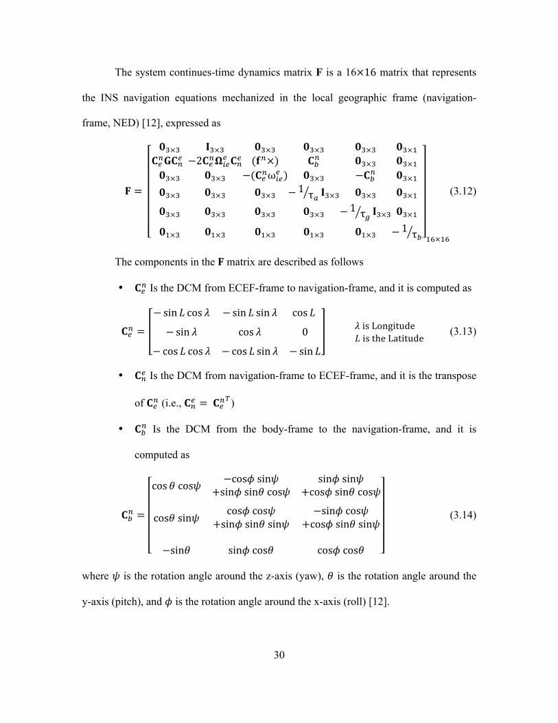
The system continues-time dynamics matrix F is a 16×16 matrix that represents

the INS navigation equations mechanized in the local geographic frame (navigation-

frame, NED) [12], expressed as

𝐅 =

𝟎!×! 𝐈!×! 𝟎!×! 𝟎!×! 𝟎!×! 𝟎!×!𝐂!!𝐆𝐂!! −2𝐂!!𝛀!"! 𝐂!! (𝐟!×) 𝐂!! 𝟎!×! 𝟎!×!𝟎!×! 𝟎!×! −(𝐂!!ω!"

! ) 𝟎!×! −𝐂!! 𝟎!×!𝟎!×! 𝟎!×! 𝟎!×! − 1 τ! 𝐈!×! 𝟎!×! 𝟎!×!𝟎!×! 𝟎!×! 𝟎!×! 𝟎!×! − 1 τ! 𝐈!×! 𝟎!×!𝟎!×! 𝟎!×! 𝟎!×! 𝟎!×! 𝟎!×! − 1 τ! !"×!"

(3.12)

The components in the 𝐅 matrix are described as follows

• 𝐂!! Is the DCM from ECEF-frame to navigation-frame, and it is computed as

𝐂!! =

− sin 𝐿 cos 𝜆 − sin 𝐿 sin 𝜆 cos 𝐿

− sin 𝜆 cos 𝜆 0

− cos 𝐿 cos 𝜆 − cos 𝐿 sin 𝜆 − sin 𝐿

𝜆 is Longitude 𝐿 is the Latitude

(3.13)

• 𝐂!! Is the DCM from navigation-frame to ECEF-frame, and it is the transpose

of 𝐂!! (i.e., 𝐂!! = 𝐂!!!)

• 𝐂!! Is the DCM from the body-frame to the navigation-frame, and it is

computed as

𝐂!! =

cos𝜃 cos𝜓 −cos𝜙 sin𝜓+sin𝜙 sin𝜃 cos𝜓

sin𝜙 sin𝜓+cos𝜙 sin𝜃 cos𝜓

cos𝜃 sin𝜓 cos𝜙 cos𝜓+sin𝜙 sin𝜃 sin𝜓

−sin𝜙 cos𝜓+cos𝜙 sin𝜃 sin𝜓

−sin𝜃 sin𝜙 cos𝜃 cos𝜙 cos𝜃

(3.14)

where 𝜓 is the rotation angle around the z-axis (yaw), 𝜃 is the rotation angle around the

y-axis (pitch), and 𝜙 is the rotation angle around the x-axis (roll) [12].

31

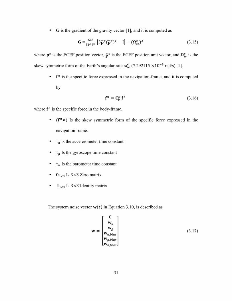
• G is the gradient of the gravity vector [1], and it is computed as

G = !"𝐏! ! 3𝐏

!(𝐏!)! − I − (𝛀!"! )! (3.15)

where 𝐩! is the ECEF position vector, 𝐏! is the ECEF position unit vector, and 𝛀!"! is the

skew symmetric form of the Earth’s angular rate ω!"! (7.292115 ×10!! rad/s) [1].

• 𝐟! is the specific force expressed in the navigation-frame, and it is computed

by

𝐟! = 𝐂!! 𝐟! (3.16)

where 𝐟! is the specific force in the body-frame.

• (𝐟!×) Is the skew symmetric form of the specific force expressed in the

navigation frame.

• τ! Is the accelerometer time constant

• τ! Is the gyroscope time constant

• τ! Is the barometer time constant

• 𝟎!×! Is 3×3 Zero matrix

• 𝐈!×! Is 3×3 Identity matrix

The system noise vector 𝐰 𝑡 in Equation 3.10, is described as

𝐰 =

0 𝐰! 𝐰!

𝐰!,!"#$𝐰!,!"#$𝐰!,!"#$

(3.17)

32

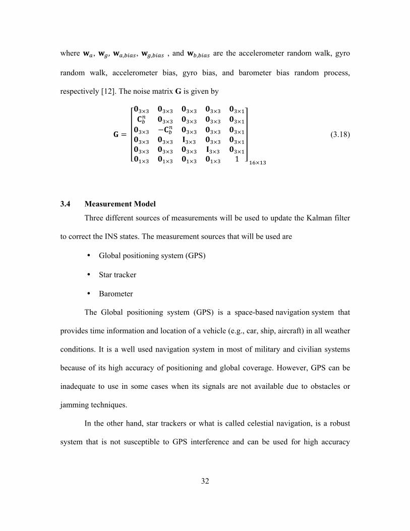
where 𝐰!, 𝐰!, 𝐰!,!"#$, 𝐰!,!"#$ , and 𝐰!,!"#$ are the accelerometer random walk, gyro

random walk, accelerometer bias, gyro bias, and barometer bias random process,

respectively [12]. The noise matrix G is given by

𝐆 =

𝟎!×! 𝟎!×! 𝟎!×! 𝟎!×! 𝟎!×!𝐂!! 𝟎!×! 𝟎!×! 𝟎!×! 𝟎!×!𝟎!×! −𝐂!! 𝟎!×! 𝟎!×! 𝟎!×!𝟎!×! 𝟎!×! 𝐈!×! 𝟎!×! 𝟎!×!𝟎!×! 𝟎!×! 𝟎!×! 𝐈!×! 𝟎!×!𝟎!×! 𝟎!×! 𝟎!×! 𝟎!×! 1 !"×!"

(3.18)

3.4 Measurement Model

Three different sources of measurements will be used to update the Kalman filter

to correct the INS states. The measurement sources that will be used are

• Global positioning system (GPS)

• Star tracker

• Barometer

The Global positioning system (GPS) is a space-based navigation system that

provides time information and location of a vehicle (e.g., car, ship, aircraft) in all weather

conditions. It is a well used navigation system in most of military and civilian systems

because of its high accuracy of positioning and global coverage. However, GPS can be

inadequate to use in some cases when its signals are not available due to obstacles or

jamming techniques.

In the other hand, star trackers or what is called celestial navigation, is a robust

system that is not susceptible to GPS interference and can be used for high accuracy

33

positioning and navigation. The last measurement source is the barometer, which is a

device used to calculate the altitude of an aircraft using the atmosphere pressure.

In general the measurement models will be expressed in the following linear form

𝐳(𝑡!) = 𝐇 𝐱(𝑡!) + 𝐯(𝑡!) (3.19)

where z(𝑡!) is the measurement vector, H is the measurement matrix and v(𝑡!) is a white

Gaussian noise with zero mean and covariance defined as [11]

𝐄[𝐯(𝑡!)𝐯!(𝑡!)] = 𝐑δ(𝑘 − 𝑗) (3.20)

where δ(𝑘 − 𝑗) is the Kronecker delta function.

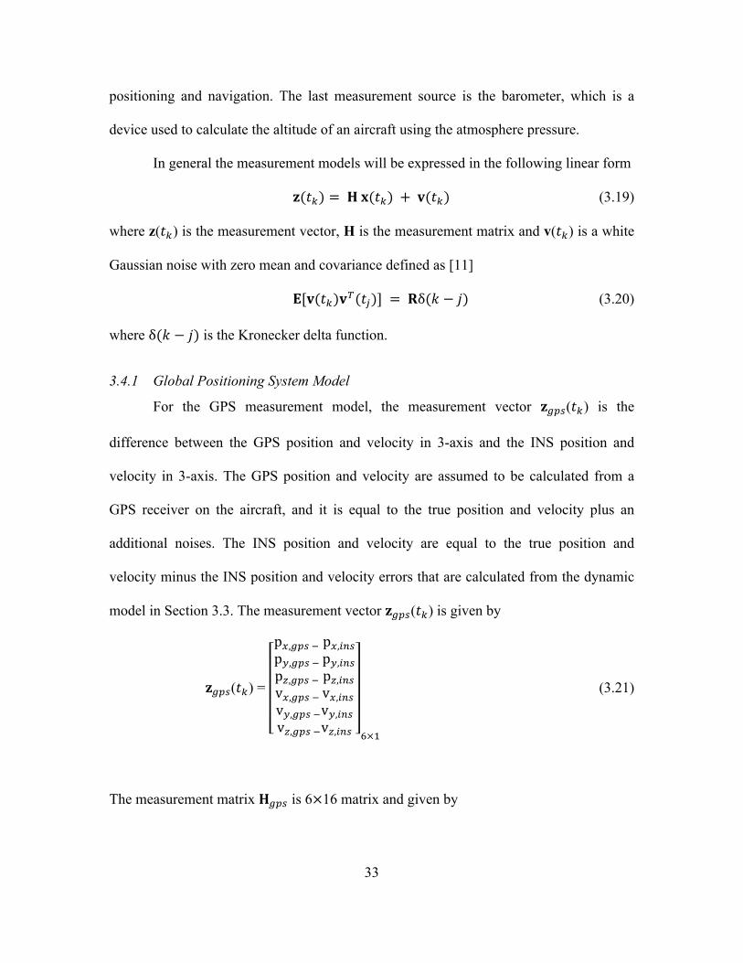
3.4.1 Global Positioning System Model

For the GPS measurement model, the measurement vector 𝐳!"#(𝑡!) is the

difference between the GPS position and velocity in 3-axis and the INS position and

velocity in 3-axis. The GPS position and velocity are assumed to be calculated from a

GPS receiver on the aircraft, and it is equal to the true position and velocity plus an

additional noises. The INS position and velocity are equal to the true position and

velocity minus the INS position and velocity errors that are calculated from the dynamic

model in Section 3.3. The measurement vector 𝐳!"#(𝑡!) is given by

𝐳!"#(𝑡!) =

p!,!"# ! p!,!"#p!,!"# ! p!,!"#p!,!"# ! p!,!"#v!,!"# ! v!,!"#v!,!"# !v!,!"#v!,!"# !v!,!"# !×!

(3.21)

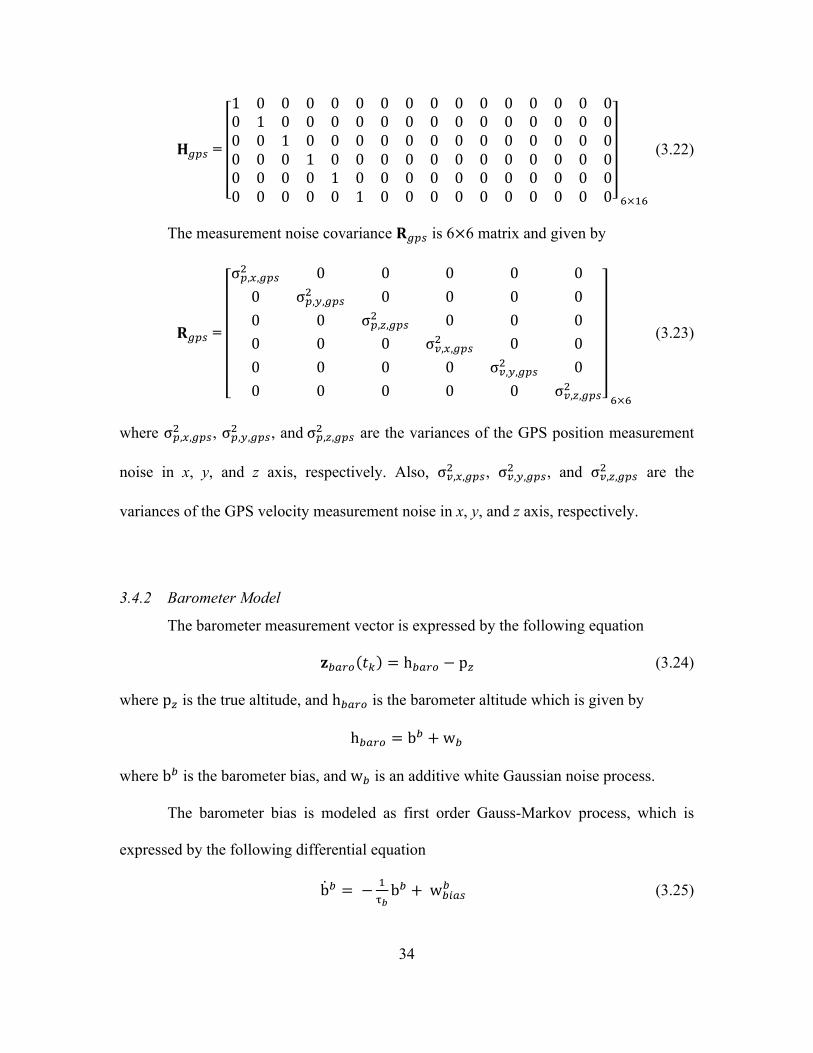
The measurement matrix 𝐇!"# is 6×16 matrix and given by

34

𝐇!"# =

1 0 0 0 0 0 0 0 0 0 0 0 0 0 0 00 1 0 0 0 0 0 0 0 0 0 0 0 0 0 00 0 1 0 0 0 0 0 0 0 0 0 0 0 0 00 0 0 1 0 0 0 0 0 0 0 0 0 0 0 00 0 0 0 1 0 0 0 0 0 0 0 0 0 0 00 0 0 0 0 1 0 0 0 0 0 0 0 0 0 0 !×!"

(3.22)

The measurement noise covariance 𝐑!"# is 6×6 matrix and given by

𝐑!"# =

σ!,!,!"#! 0 0 0 0 00 σ!,!,!"#! 0 0 0 00 0 σ!,!,!"#! 0 0 00 0 0 σ!,!,!"#! 0 00 0 0 0 σ!,!,!"#! 00 0 0 0 0 σ!,!,!"#!

!×!

(3.23)

where σ!,!,!"#! , σ!,!,!"#! , and σ!,!,!"#! are the variances of the GPS position measurement

noise in x, y, and z axis, respectively. Also, σ!,!,!"#! , σ!,!,!"#! , and σ!,!,!"#! are the

variances of the GPS velocity measurement noise in x, y, and z axis, respectively.

3.4.2 Barometer Model

The barometer measurement vector is expressed by the following equation

𝐳!"#$ 𝑡! = h!"#$ − p! (3.24)

where p! is the true altitude, and h!"#$ is the barometer altitude which is given by

h!"#$ = b! +w!

where b! is the barometer bias, and w! is an additive white Gaussian noise process.

The barometer bias is modeled as first order Gauss-Markov process, which is

expressed by the following differential equation

b! = − !!!b! + w!"#$

! (3.25)

35

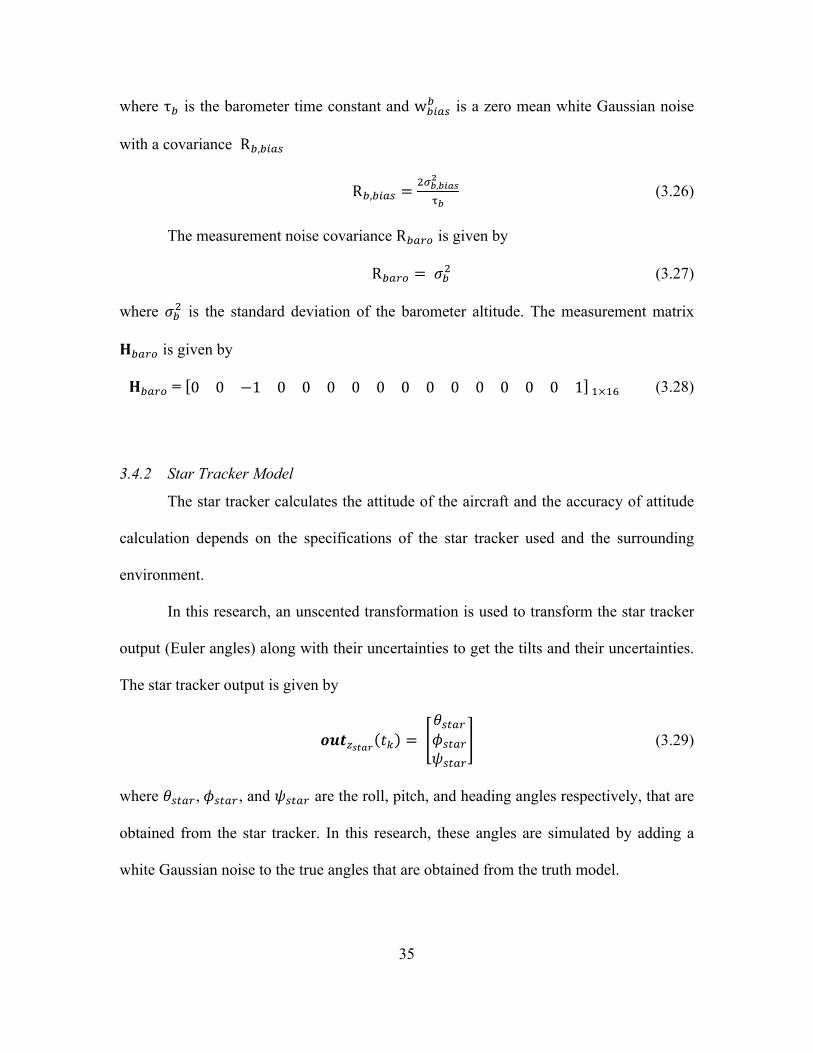
where τ! is the barometer time constant and w!!"#! is a zero mean white Gaussian noise

with a covariance R!,!"#$

R!,!"#$ =!!!,!"#$

!

!! (3.26)

The measurement noise covariance R!"#$ is given by

R!"#$ = 𝜎!! (3.27)

where 𝜎!! is the standard deviation of the barometer altitude. The measurement matrix

𝐇!"#$ is given by

𝐇!"#$ = 0 0 −1 0 0 0 0 0 0 0 0 0 0 0 0 1 !×!" (3.28)

3.4.2 Star Tracker Model

The star tracker calculates the attitude of the aircraft and the accuracy of attitude

calculation depends on the specifications of the star tracker used and the surrounding

environment.

In this research, an unscented transformation is used to transform the star tracker

output (Euler angles) along with their uncertainties to get the tilts and their uncertainties.

The star tracker output is given by

𝒐𝒖𝒕!!"#$ 𝑡! = 𝜃!"#$𝜙!"#$𝜓!"#$

(3.29)

where 𝜃!"#$, 𝜙!"#$, and 𝜓!"#$ are the roll, pitch, and heading angles respectively, that are

obtained from the star tracker. In this research, these angles are simulated by adding a

white Gaussian noise to the true angles that are obtained from the truth model.

36

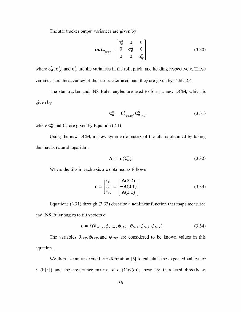
The star tracker output variances are given by

𝒐𝒖𝒕!!"#$ = σ!! 0 00 σ!! 00 0 σ!!

(3.30)

where σ!! , σ!! , and σ!! are the variances in the roll, pitch, and heading respectively. These

variances are the accuracy of the star tracker used, and they are given by Table 2.4.

The star tracker and INS Euler angles are used to form a new DCM, which is

given by

𝐂!! = 𝐂!!!"#$ .𝐂!!!"# (3.31)

where 𝐂!! and 𝐂!! are given by Equation (2.1).

Using the new DCM, a skew symmetric matrix of the tilts is obtained by taking

the matrix natural logarithm

𝐀 = ln(𝐂!!) (3.32)

Where the tilts in each axis are obtained as follows

𝝐 =𝜖!𝜖!𝜖!

=𝐀(3,2)−𝐀(3,1)𝐀(2,1)

(3.33)

Equations (3.31) through (3.33) describe a nonlinear function that maps measured

and INS Euler angles to tilt vectors 𝝐

𝝐 = 𝑓(𝜃!"#$ ,𝜙!"#$ ,𝜓!"!" ,𝜃!"#,𝜙!"#,𝜓!"#) (3.34)

The variables 𝜃!"#,𝜙!"#, and 𝜓!"# are considered to be known values in this

equation.

We then use an unscented transformation [6] to calculate the expected values for

𝝐 (Ε 𝝐 ) and the covariance matrix of 𝝐 (Cov(𝝐)), these are then used directly as

37

measurements in the Kalman filter. Therefore, the star tracker measurement vector and

covariance matrix are given by

𝐳!"#$ 𝑡! = Ε 𝝐 (3.35)

𝐑!"#$ = Cov(𝝐) (3.36)

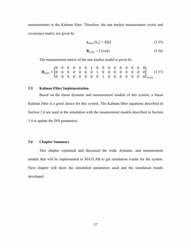
The measurement matrix of the star tracker model is given by

𝐇!"#$ = 0 0 0 0 0 0 1 0 0 0 0 0 0 0 0 00 0 0 0 0 0 0 1 0 0 0 0 0 0 0 00 0 0 0 0 0 0 0 1 0 0 0 0 0 0 0 !×!"

(3.37)

3.5 Kalman Filter Implementation

Based on the linear dynamic and measurement models of this system, a linear

Kalman filter is a good choice for this system. The Kalman filter equations described in

Section 2.6 are used in the simulation with the measurement models described in Section

3.4 to update the INS parameters.

3.6 Chapter Summary

This chapter explained and discussed the truth, dynamic, and measurement

models that will be implemented in MATLAB to get simulation results for the system.

Next chapter will show the simulation parameters used and the simulation results

developed.

38

IV. Simulation Results

n this chapter, simulated performance results for the methodology discussed in the

previous chapter will be shown and analyzed. We will start with explaining the

different INS grades that will be used in the simulation along with their parameters. Next,

simulation scenarios will be explained. Then, a Kalman filter validation step will be

shown. Then in the following sections, results of different scenarios including GPS, star

tracker and barometer aiding is presented and analyzed.

There are three different grades of INS; commercial, tactical and navigation. The

commercial grade INS has low quality sensors (i.e. Accelerometers and Gyroscopes) and

these sensors should be calibrated after installation in the Inertial Measurement Unit

(IMU) to be used for short duration flights. In contrast, tactical grade INS is a medium

quality grade that is used for medium flight durations of several minutes. Finally, the

navigation grade INS is used for long flight durations and has good quality sensors. Key

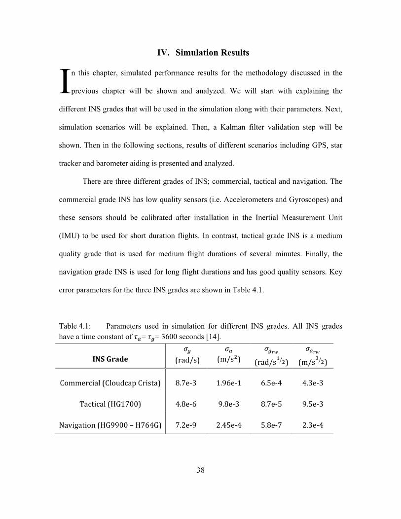
error parameters for the three INS grades are shown in Table 4.1.

Table 4.1: Parameters used in simulation for different INS grades. All INS grades have a time constant of 𝜏!= 𝜏!= 3600 seconds [14].

INS Grade

𝜎! (rad/s)

𝜎! (m/s!)

𝜎!!"

(rad/s! !)

𝜎!!"

(m/s! !)

Commercial (Cloudcap Crista)

8.7e-‐3

1.96e-‐1

6.5e-‐4

4.3e-‐3

Tactical (HG1700)

4.8e-‐6

9.8e-‐3

8.7e-‐5

9.5e-‐3

Navigation (HG9900 – H764G)

7.2e-‐9

2.45e-‐4

5.8e-‐7

2.3e-‐4

I

39

In Table 4.1, the gyroscope time-correlated bias time constant is denoted by 𝜏!,

the accelerometer time-correlated bias time constant is denoted by 𝜏!, the gyroscope

time-correlated bias standard deviation is denoted by 𝜎!, and the accelerometer time-

correlated bias standard deviation is denoted by 𝜎!. Also, the accelerometer and

gyroscope random walk noise strength is denoted by 𝜎!!" and 𝜎!!", respectively [14].

The flight dynamics and duration limits the criteria of selecting the inertial grade

needed for the application. In the research, the previous discussed INS grades will be

simulated for different flight durations depending on the INS grade used and the result

analysis. In addition, the flight dynamics is assumed to be a normally straight and level

flight with no maneuvers and very little acceleration.

4.1 Simulation Scenarios

In the following sections of this chapter, there are two scenarios selected to

compare between the different measurements models described in chapter III. The two

scenarios are as follows

• Scenario one: GPS initialization, Star tracker and Barometer.

• Scenario two: GPS initialization and Barometer.

In the first scenario, GPS, star tracker, and barometer measurements will be used

from the beginning of the flight but the GPS will be only for the first 200 seconds. The

second scenario will be like the first scenario but without the star tracker. Table 4.2

descries the star tracker parameters used in the research, which were obtained from [13].

40

Table 4.2: Star Tracker Parameters Star Tracker Name SUNSAT Star Tracker

Roll Accuracy 12 arcseconds

Pitch Accuracy 12 arcseconds

Yaw Accuracy 12 arcseconds

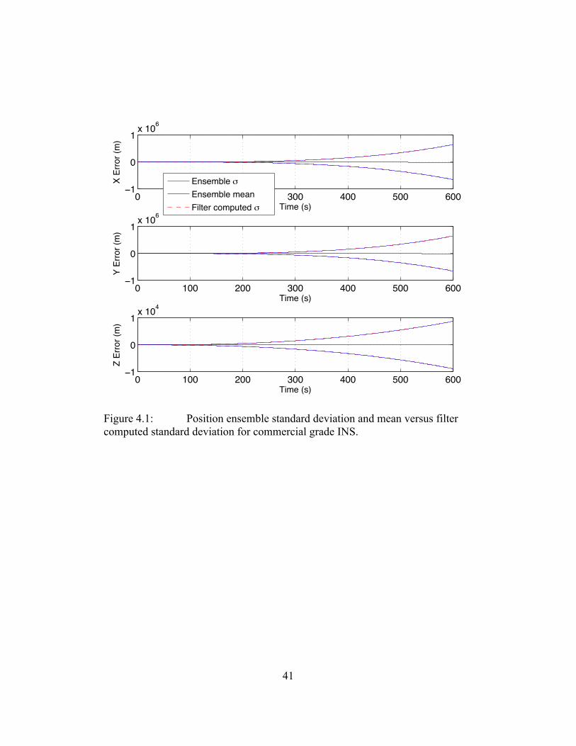
4.2 Filter Validation

This section contains simulated navigation results using the INS model developed

in Section 3.3 and the measurement models developed in Section 3.4. The simulations in

this section use the INS parameters from Table 4.1, the star tracker parameters from

Table 4.2, and the navigation parameters from Table 4.3.

Before developing the results, Kalman filter validation is an important step to

verify that the filter is well designed and can estimate the states needed for this research.

The filter validation is carried out through simulation of 1000 Monte Carlo runs for the

three INS grades.

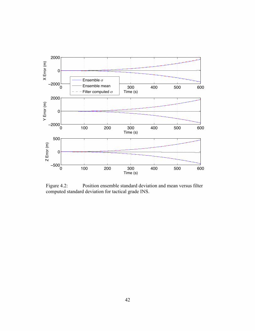
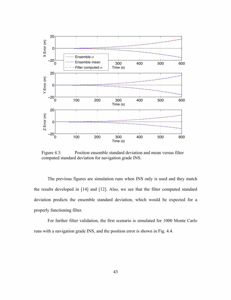
Figures 4.1, 4.2, and 4.3 show the Monte Carlo runs for the position error for the

commercial grade INS, tactical grade INS, and navigation grade INS, respectively.

Table 4.3: Simulation Parameters for Navigation Filter

Kalman Filter Propagation Time 1 second

Initial Position (0,0,0) m

Initial Velocity (200,0,0) m/s

Initial Acceleration (0,0,0) m/s!

41

Figure 4.1: Position ensemble standard deviation and mean versus filter computed standard deviation for commercial grade INS.

0 100 200 300 400 500 600−1

0

1x 106

Time (s)

X Er

ror (

m)

Ensemble mEnsemble meanFilter computed m

0 100 200 300 400 500 600−1

0

1x 106

Time (s)

Y Er

ror (

m)

0 100 200 300 400 500 600−1

0

1x 104

Time (s)

Z Er

ror (

m)

42

Figure 4.2: Position ensemble standard deviation and mean versus filter computed standard deviation for tactical grade INS.

0 100 200 300 400 500 600−2000

0

2000

Time (s)

X Er

ror (

m)


0 100 200 300 400 500 600−2000

0

2000

Time (s)

Y Er

ror (

m)

0 100 200 300 400 500 600−500

0

500

Time (s)

Z Er

ror (

m)

43

Figure 4.3: Position ensemble standard deviation and mean versus filter computed standard deviation for navigation grade INS.

The previous figures are simulation runs when INS only is used and they match

the results developed in [14] and [12]. Also, we see that the filter computed standard

deviation predicts the ensemble standard deviation, which would be expected for a

properly functioning filter.

For further filter validation, the first scenario is simulated for 1000 Monte Carlo

runs with a navigation grade INS, and the position error is shown in Fig. 4.4.

0 100 200 300 400 500 600−20

0

20

Time (s)

X Er

ror (

m)


0 100 200 300 400 500 600−20

0

20

Time (s)

Y Er

ror (

m)

0 100 200 300 400 500 600−20

0

20

Time (s)

Z Er

ror (

m)

44

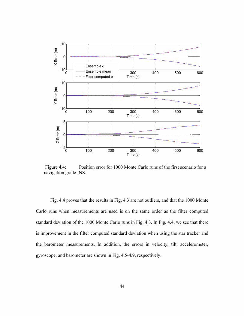
Figure 4.4: Position error for 1000 Monte Carlo runs of the first scenario for a navigation grade INS.

Fig. 4.4 proves that the results in Fig. 4.3 are not outliers, and that the 1000 Monte

Carlo runs when measurements are used is on the same order as the filter computed

standard deviation of the 1000 Monte Carlo runs in Fig. 4.3. In Fig. 4.4, we see that there

is improvement in the filter computed standard deviation when using the star tracker and

the barometer measurements. In addition, the errors in velocity, tilt, accelerometer,

gyroscope, and barometer are shown in Fig. 4.5-4.9, respectively.

0 100 200 300 400 500 600−10

0

10

Time (s)

X Er

ror (

m)


0 100 200 300 400 500 600−10

0

10

Time (s)

Y Er

ror (

m)

0 100 200 300 400 500 600−5

0

5

Time (s)

Z Er

ror (

m)

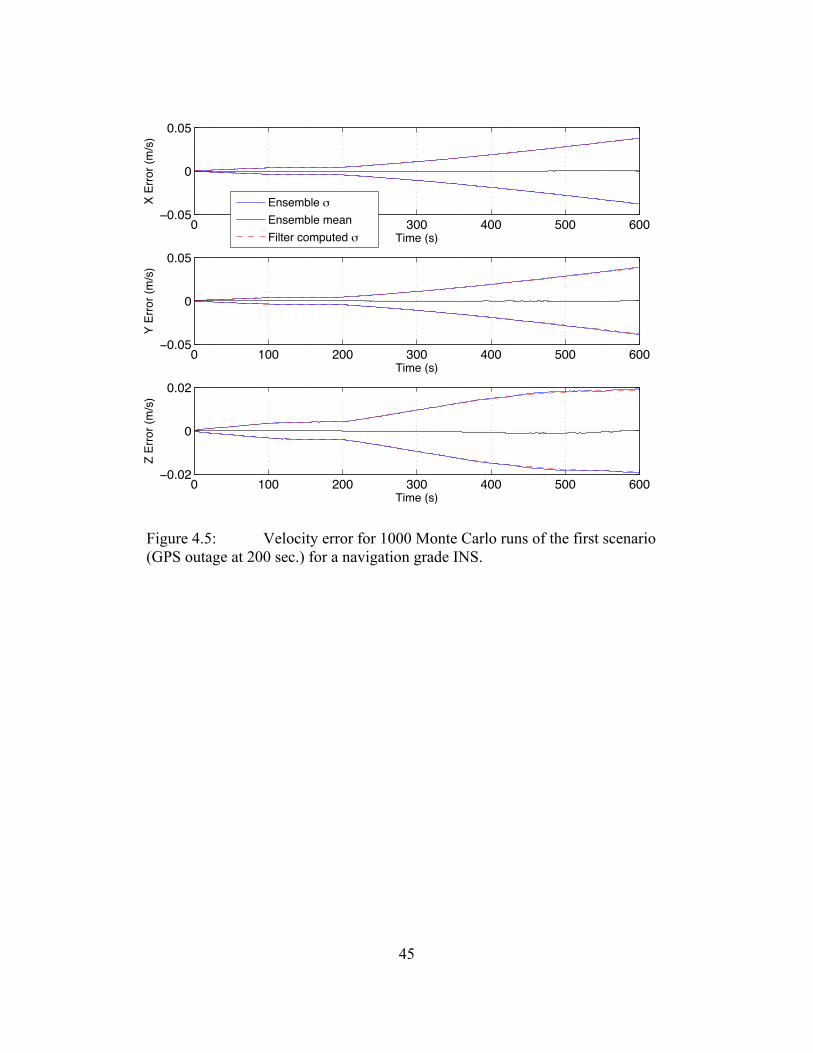
45

Figure 4.5: Velocity error for 1000 Monte Carlo runs of the first scenario (GPS outage at 200 sec.) for a navigation grade INS.

0 100 200 300 400 500 600−0.05

0

0.05

Time (s)

X Er

ror (

m/s

)


0 100 200 300 400 500 600−0.05

0

0.05

Time (s)

Y Er

ror (

m/s

)

0 100 200 300 400 500 600−0.02

0

0.02

Time (s)

Z Er

ror (

m/s

)

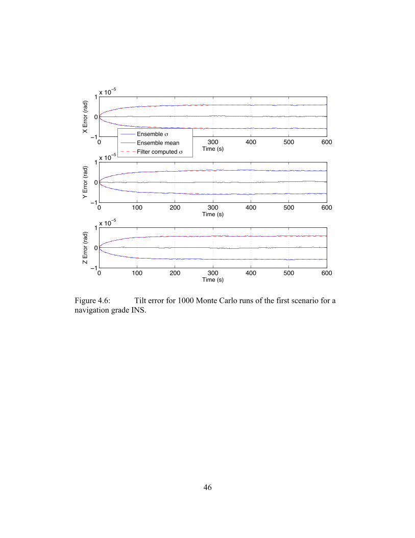
46

Figure 4.6: Tilt error for 1000 Monte Carlo runs of the first scenario for a navigation grade INS.

0 100 200 300 400 500 600−1

0

1x 10−5

Time (s)

X Er

ror (

rad)


0 100 200 300 400 500 600−1

0

1x 10−5

Time (s)

Y Er

ror (

rad)

0 100 200 300 400 500 600−1

0

1x 10−5

Time (s)

Z Er

ror (

rad)

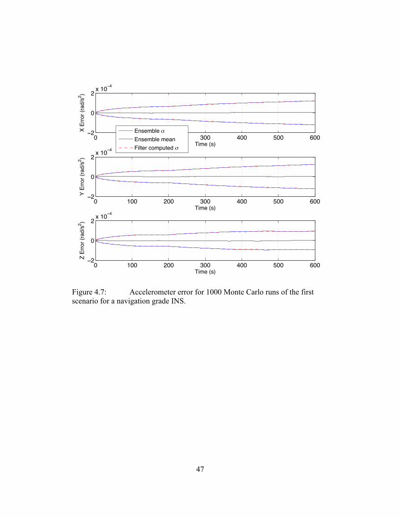
47

Figure 4.7: Accelerometer error for 1000 Monte Carlo runs of the first scenario for a navigation grade INS.

0 100 200 300 400 500 600−2

0

2x 10−4

Time (s)

X Er

ror (

rad/

s2 )


0 100 200 300 400 500 600−2

0

2x 10−4

Time (s)

Y Er

ror (

rad/

s2 )

0 100 200 300 400 500 600−2

0

2x 10−4

Time (s)

Z Er

ror (

rad/

s2 )

48

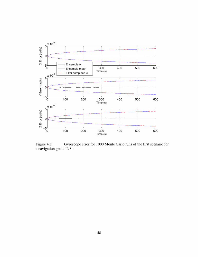
Figure 4.8: Gyroscope error for 1000 Monte Carlo runs of the first scenario for a navigation grade INS.

0 100 200 300 400 500 600−5

0

5x 10−9

Time (s)

X Er

ror (

rad/

s)


0 100 200 300 400 500 600−5

0

5x 10−9

Time (s)

Y Er

ror (

rad/

s)

0 100 200 300 400 500 600−5

0

5x 10−9

Time (s)

Z Er

ror (

rad/

s)

49

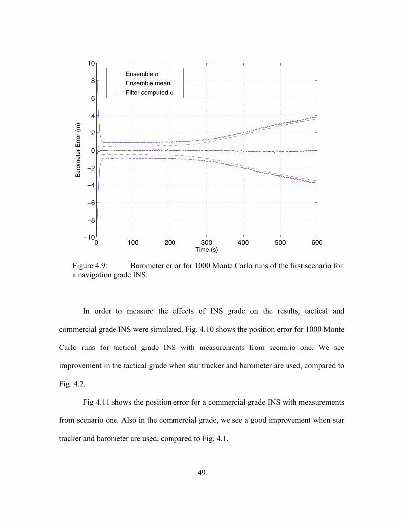
Figure 4.9: Barometer error for 1000 Monte Carlo runs of the first scenario for a navigation grade INS.

In order to measure the effects of INS grade on the results, tactical and

commercial grade INS were simulated. Fig. 4.10 shows the position error for 1000 Monte

Carlo runs for tactical grade INS with measurements from scenario one. We see

improvement in the tactical grade when star tracker and barometer are used, compared to

Fig. 4.2.

Fig 4.11 shows the position error for a commercial grade INS with measurements

from scenario one. Also in the commercial grade, we see a good improvement when star

tracker and barometer are used, compared to Fig. 4.1.

0 100 200 300 400 500 600−10

−8

−6

−4

−2

0

2

4

6

8

10

Time (s)

Baro

met

er E

rror (

m)


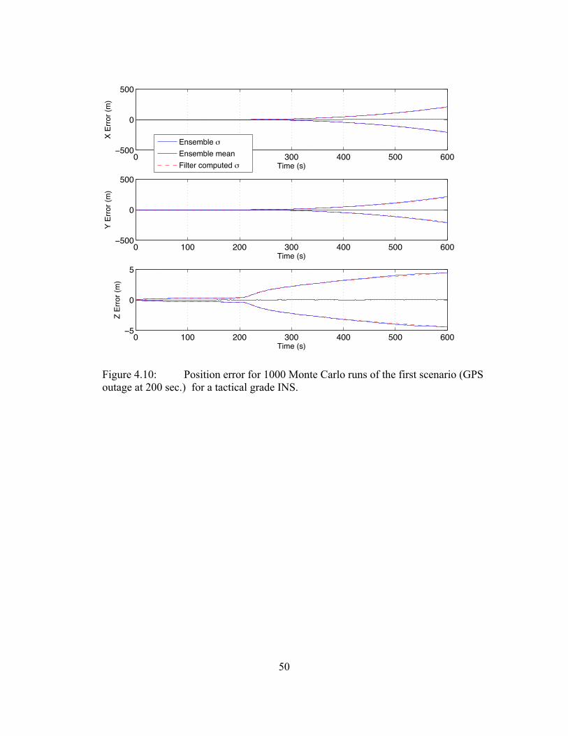
50

Figure 4.10: Position error for 1000 Monte Carlo runs of the first scenario (GPS outage at 200 sec.) for a tactical grade INS.

0 100 200 300 400 500 600−500

0

500

Time (s)

X Er

ror (

m)


0 100 200 300 400 500 600−500

0

500

Time (s)

Y Er

ror (

m)

0 100 200 300 400 500 600−5

0

5

Time (s)

Z Er

ror (

m)

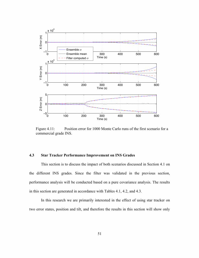
51

Figure 4.11: Position error for 1000 Monte Carlo runs of the first scenario for a commercial grade INS.

4.3 Star Tracker Performance Improvement on INS Grades

This section is to discuss the impact of both scenarios discussed in Section 4.1 on

the different INS grades. Since the filter was validated in the previous section,

performance analysis will be conducted based on a pure covariance analysis. The results

in this section are generated in accordance with Tables 4.1, 4.2, and 4.3.

In this research we are primarily interested in the effect of using star tracker on

two error states, position and tilt, and therefore the results in this section will show only

0 100 200 300 400 500 600−1

0

1x 104

Time (s)

X Er

ror (

m)


0 100 200 300 400 500 600−1

0

1x 104

Time (s)

Y Er

ror (

m)

0 100 200 300 400 500 600−5

0

5

Time (s)

Z Er

ror (

m)

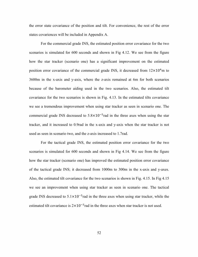
52

the error state covariance of the position and tilt. For convenience, the rest of the error

states covariences will be included in Appendix A.

For the commercial grade INS, the estimated position error covariance for the two

scenarios is simulated for 600 seconds and shown in Fig 4.12. We see from the figure

how the star tracker (scenario one) has a significant improvement on the estimated

position error covariance of the commercial grade INS, it decreased from 12×10!m to

3600m in the x-axis and y-axis, where the z-axis remained at 6m for both scenarios

because of the barometer aiding used in the two scenarios. Also, the estimated tilt

covariance for the two scenarios is shown in Fig. 4.13. In the estimated tilts covariance

we see a tremendous improvement when using star tracker as seen in scenario one. The

commercial grade INS decreased to 5.8×10!!rad in the three axes when using the star

tracker, and it increased to 0.9rad in the x-axis and y-axis when the star tracker is not

used as seen in scenario two, and the z-axis increased to 1.7rad.

For the tactical grade INS, the estimated position error covariance for the two

scenarios is simulated for 600 seconds and shown in Fig 4.14. We see from the figure

how the star tracker (scenario one) has improved the estimated position error covariance

of the tactical grade INS; it decreased from 1000m to 300m in the x-axis and y-axes.

Also, the estimated tilt covariance for the two scenarios is shown in Fig. 4.15. In Fig 4.15

we see an improvement when using star tracker as seen in scenario one. The tactical

grade INS decreased to 5.1×10!!rad in the three axes when using star tracker, while the

estimated tilt covariance is 2×10!!rad in the three axes when star tracker is not used.

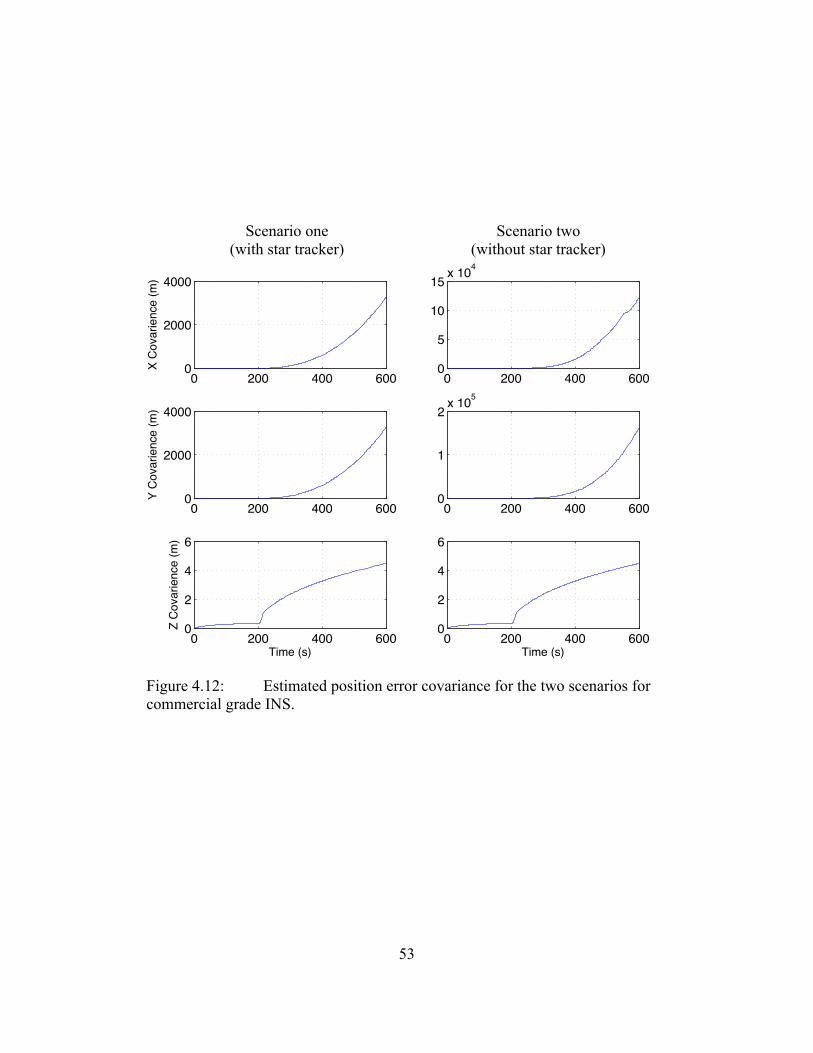
53

Figure 4.12: Estimated position error covariance for the two scenarios for commercial grade INS.

0 200 400 6000

2000

4000

X C

ovar

ienc

e (m

)

0 200 400 6000

2000

4000

Y C

ovar

ienc

e (m

)

0 200 400 6000

2

4

6

Time (s)

Z C

ovar

ienc

e (m

)

0 200 400 6000

5

10

15x 104

0 200 400 6000

1

2x 105

0 200 400 6000

2

4

6

Time (s)

Scenario one (with star tracker)

Scenario two (without star tracker)

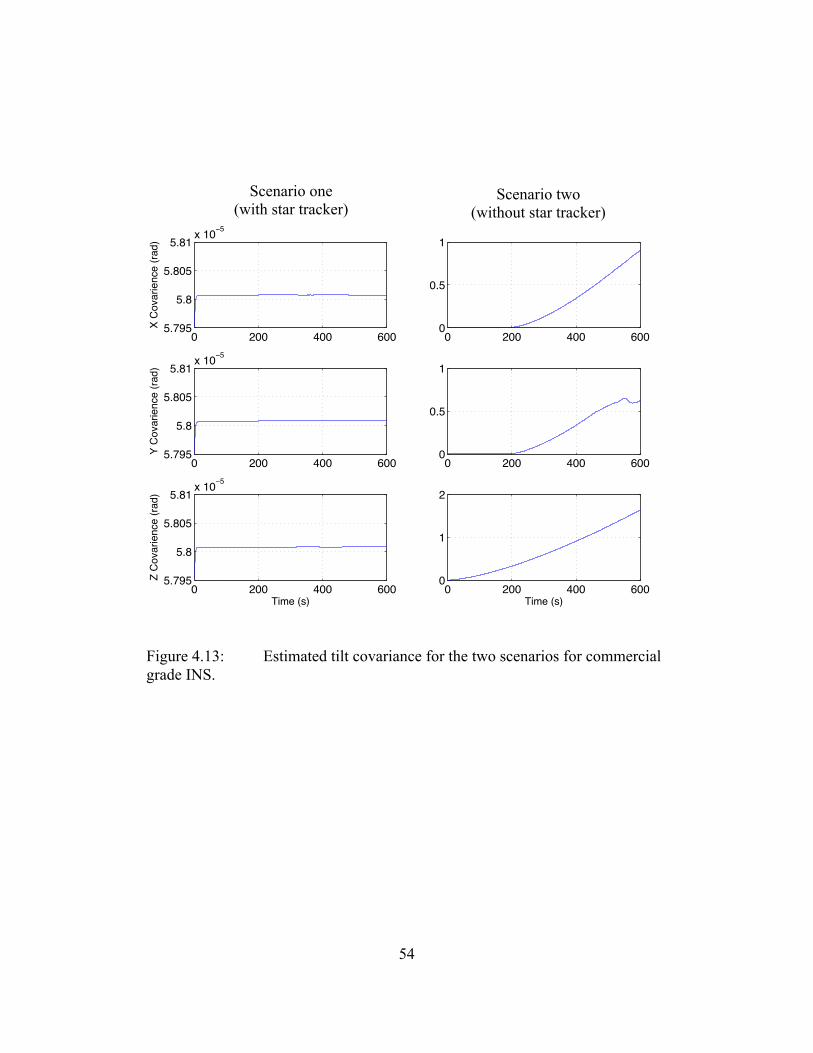
54

Figure 4.13: Estimated tilt covariance for the two scenarios for commercial grade INS.

0 200 400 6005.795

5.8

5.805

5.81x 10−5

X C

ovar

ienc

e (ra

d)

0 200 400 6005.795

5.8

5.805

5.81x 10−5

Y C

ovar

ienc

e (ra

d)

0 200 400 6005.795

5.8

5.805

5.81x 10−5

Time (s)

Z C

ovar

ienc

e (ra

d)

0 200 400 6000

0.5

1

0 200 400 6000

0.5

1

0 200 400 6000

1

2

Time (s)



55

Figure 4.14: Estimated position error covariance for the two scenarios for tactical grade INS.

0 200 400 6000

100

200

300

X C

ovar

ienc

e (m

)

0 200 400 6000

100

200

300

Y C

ovar

ienc

e (m

)

0 200 400 6000

2

4

6

Time (s)

Z C

ovar

ienc

e (m

)

0 200 400 6000

500

1000

0 200 400 6000

500

1000

0 200 400 6000

2

4

6

Time (s)



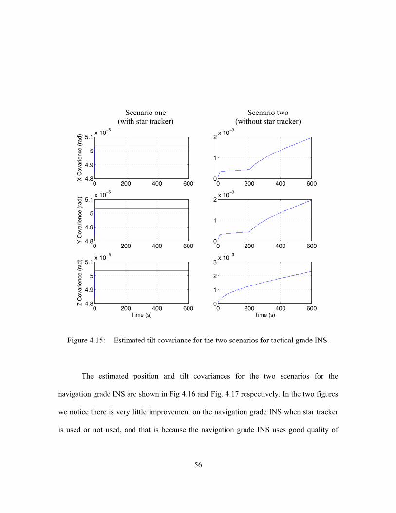
56

Figure 4.15: Estimated tilt covariance for the two scenarios for tactical grade INS.

The estimated position and tilt covariances for the two scenarios for the

navigation grade INS are shown in Fig 4.16 and Fig. 4.17 respectively. In the two figures

we notice there is very little improvement on the navigation grade INS when star tracker

is used or not used, and that is because the navigation grade INS uses good quality of

0 200 400 6004.8

4.9

5

5.1x 10−5

X C

ovar

ienc

e (ra

d)

0 200 400 6004.8

4.9

5

5.1x 10−5

Y C

ovar

ienc

e (ra

d)

0 200 400 6004.8

4.9

5

5.1x 10−5

Time (s)

Z C

ovar

ienc

e (ra

d)

0 200 400 6000

1

2x 10−3

0 200 400 6000

1

2x 10−3

0 200 400 6000

1

2

3x 10−3

Time (s)



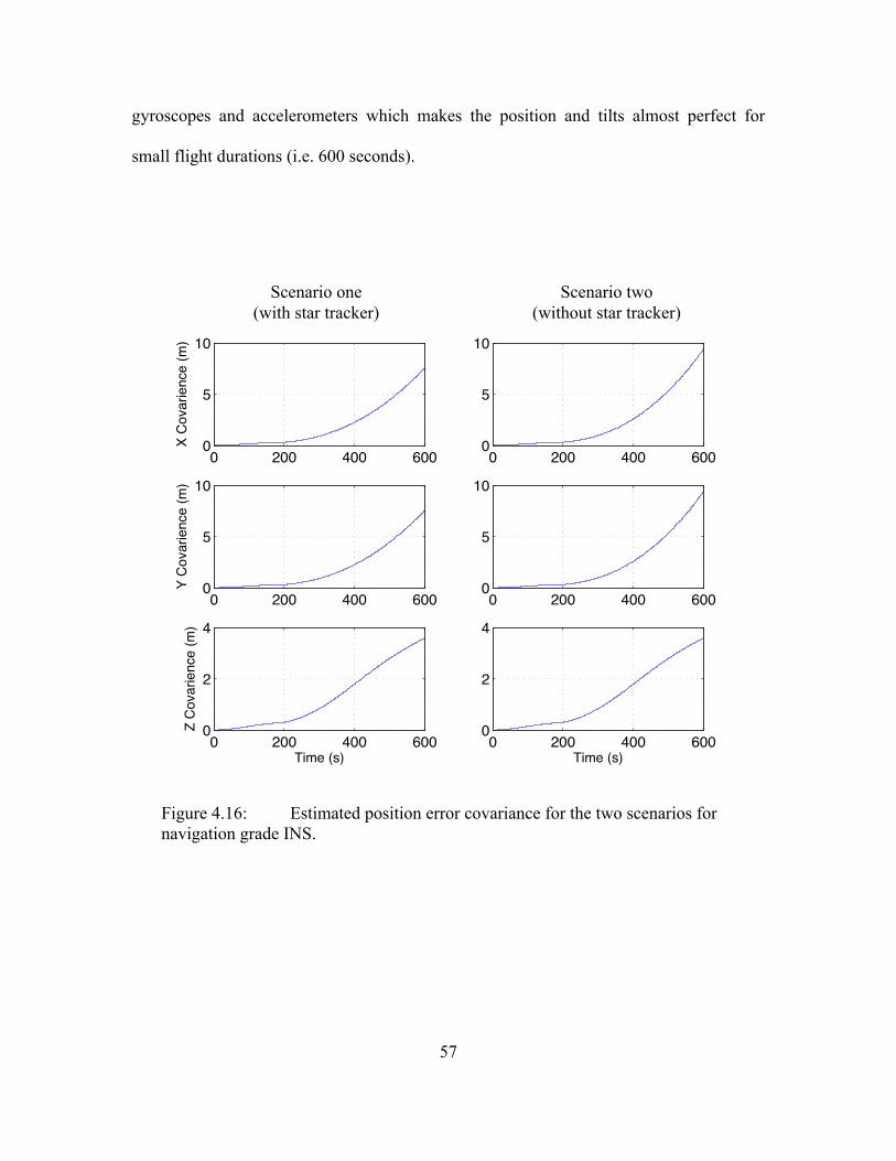
57

gyroscopes and accelerometers which makes the position and tilts almost perfect for

small flight durations (i.e. 600 seconds).

Figure 4.16: Estimated position error covariance for the two scenarios for navigation grade INS.

0 200 400 6000

5

10

X C

ovar

ienc

e (m

)

0 200 400 6000

5

10

Y C

ovar

ienc

e (m

)

0 200 400 6000

2

4

Time (s)

Z C

ovar

ienc

e (m

)

0 200 400 6000

5

10

0 200 400 6000

5

10

0 200 400 6000

2

4

Time (s)



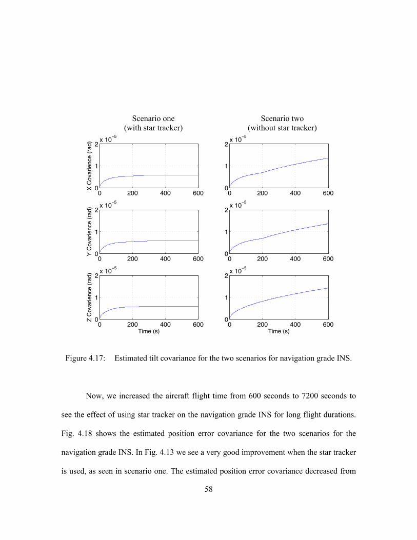
58

Figure 4.17: Estimated tilt covariance for the two scenarios for navigation grade INS.

Now, we increased the aircraft flight time from 600 seconds to 7200 seconds to

see the effect of using star tracker on the navigation grade INS for long flight durations.

Fig. 4.18 shows the estimated position error covariance for the two scenarios for the

navigation grade INS. In Fig. 4.13 we see a very good improvement when the star tracker

is used, as seen in scenario one. The estimated position error covariance decreased from

0 200 400 6000

1

2x 10−5

X C

ovar

ienc

e (ra

d)

0 200 400 6000

1

2x 10−5

Y C

ovar

ienc

e (ra

d)

0 200 400 6000

1

2x 10−5

Time (s)

Z C

ovar

ienc

e (ra

d)

0 200 400 6000

1

2x 10−5

0 200 400 6000

1

2x 10−5

0 200 400 6000

1

2x 10−5

Time (s)



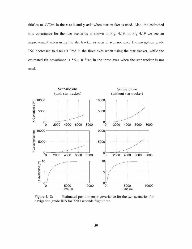
59

6603m to 3370m in the x-axis and y-axis when star tracker is used. Also, the estimated

tilts covariance for the two scenarios is shown in Fig. 4.19. In Fig 4.19 we see an

improvement when using the star tracker as seen in scenario one. The navigation grade

INS decreased to 5.8×10!!rad in the three axes when using the star tracker, while the

estimated tilt covariance is 5.9×10!!rad in the three axes when the star tracker is not

used.

Figure 4.18: Estimated position error covariance for the two scenarios for navigation grade INS for 7200 seconds flight time.

0 2000 4000 6000 80000

5000

10000

X C

ovar

ienc

e (m

)

0 2000 4000 6000 80000

5000

10000

Y C

ovar

ienc

e (m

)

0 5000 100000

5

10

Time (s)

Z C

ovar

ienc

e (m

)

0 2000 4000 6000 80000

5000

10000

0 2000 4000 6000 80000

5000

10000

0 5000 100000

5

10

Time (s)



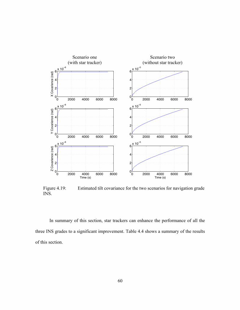
60

Figure 4.19: Estimated tilt covariance for the two scenarios for navigation grade INS.

In summary of this section, star trackers can enhance the performance of all the

three INS grades to a significant improvement. Table 4.4 shows a summary of the results

of this section.

0 2000 4000 6000 80000

2

4

6x 10−6

X C

ovar

ienc

e (ra

d)

0 2000 4000 6000 80000

2

4

6x 10−6

Y C

ovar

ienc

e (ra

d)

0 2000 4000 6000 80000

2

4

6x 10−6

Time (s)

Z C

ovar

ienc

e (ra

d)

0 2000 4000 6000 80000

2

4

6x 10−5

0 2000 4000 6000 80000

2

4

6x 10−5

0 2000 4000 6000 80000

2

4

6x 10−5

Time (s)



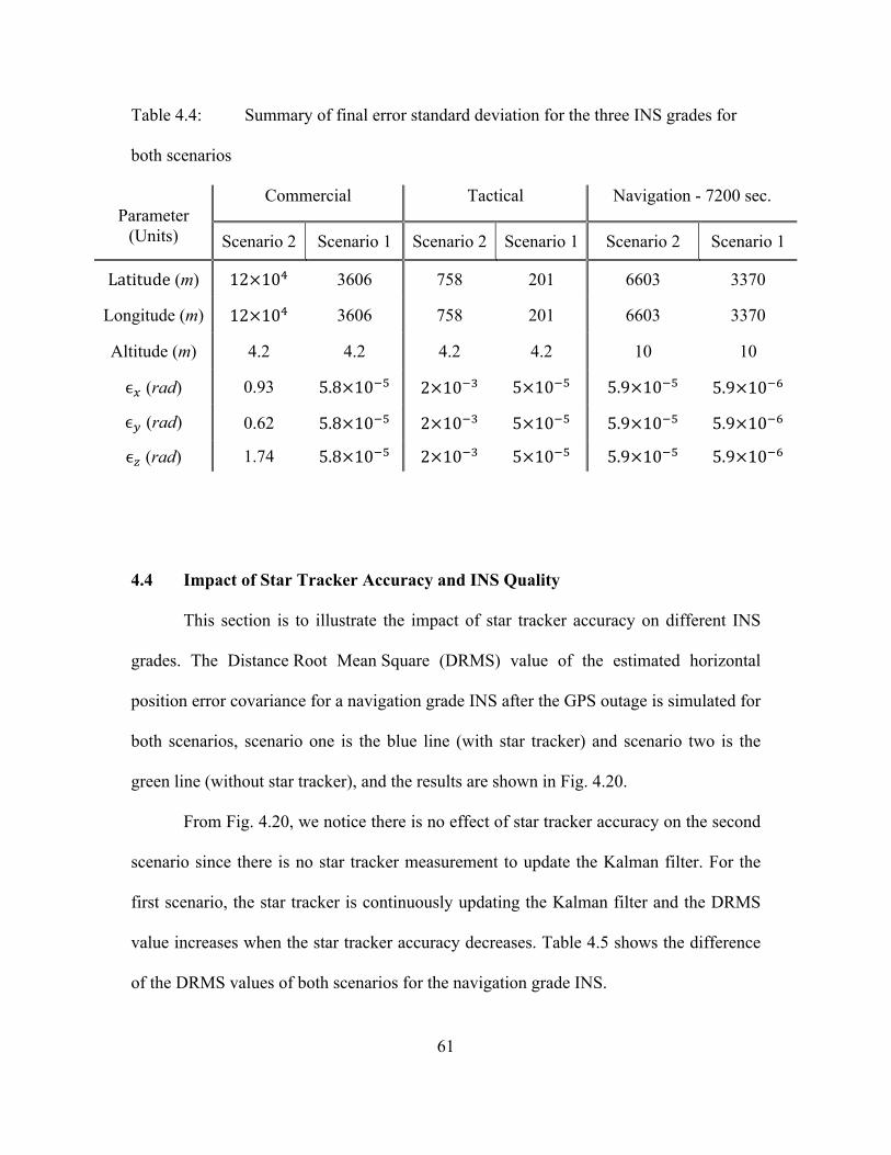
61

Table 4.4: Summary of final error standard deviation for the three INS grades for

both scenarios

Parameter

(Units)

Commercial Tactical Navigation - 7200 sec.

Scenario 2 Scenario 1 Scenario 2 Scenario 1 Scenario 2 Scenario 1

Latitude (m) 12×10! 3606 758 201 6603 3370

Longitude (m) 12×10! 3606 758 201 6603 3370

Altitude (m) 4.2 4.2 4.2 4.2 10 10

ϵ! (rad) 0.93 5.8×10!! 2×10!! 5×10!! 5.9×10!! 5.9×10!!

ϵ! (rad) 0.62 5.8×10!! 2×10!! 5×10!! 5.9×10!! 5.9×10!!

ϵ! (rad) 1.74 5.8×10!! 2×10!! 5×10!! 5.9×10!! 5.9×10!!

4.4 Impact of Star Tracker Accuracy and INS Quality

This section is to illustrate the impact of star tracker accuracy on different INS

grades. The Distance Root Mean Square (DRMS) value of the estimated horizontal

position error covariance for a navigation grade INS after the GPS outage is simulated for

both scenarios, scenario one is the blue line (with star tracker) and scenario two is the

green line (without star tracker), and the results are shown in Fig. 4.20.

From Fig. 4.20, we notice there is no effect of star tracker accuracy on the second

scenario since there is no star tracker measurement to update the Kalman filter. For the

first scenario, the star tracker is continuously updating the Kalman filter and the DRMS

value increases when the star tracker accuracy decreases. Table 4.5 shows the difference

of the DRMS values of both scenarios for the navigation grade INS.

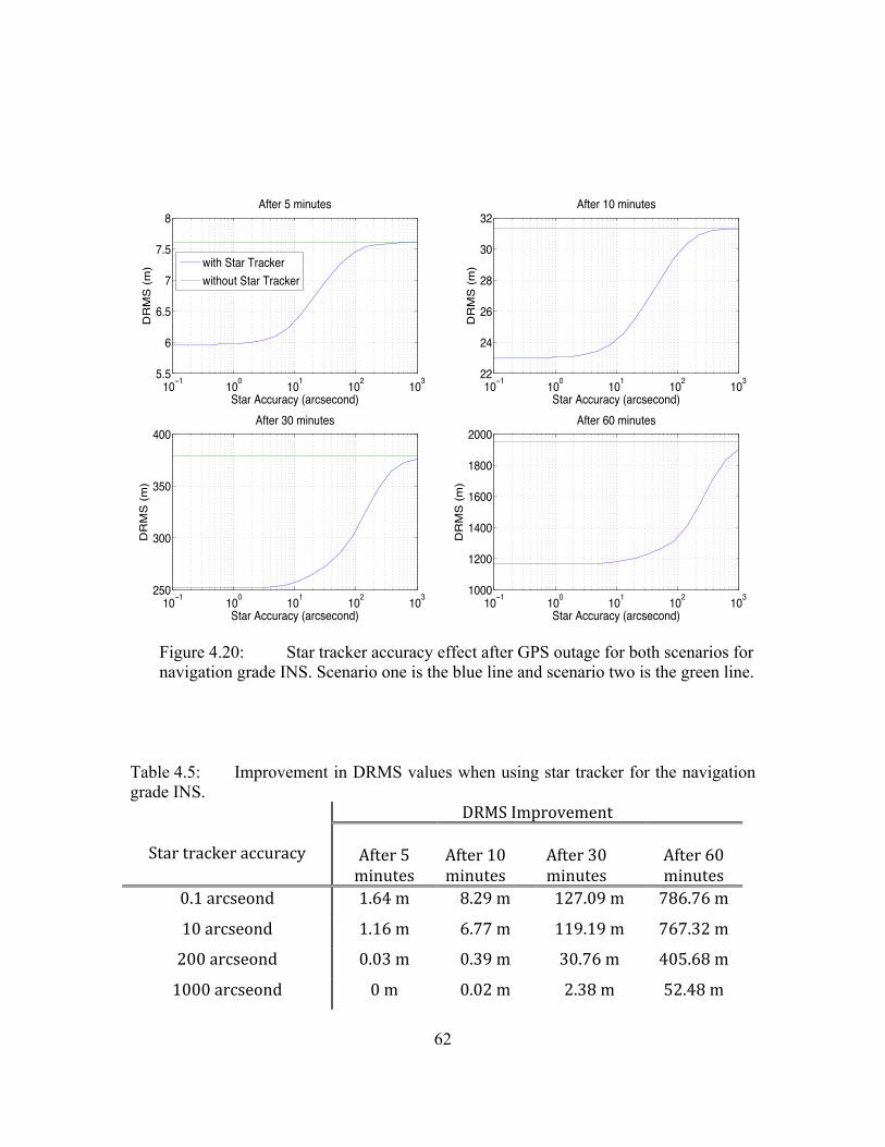
62

Figure 4.20: Star tracker accuracy effect after GPS outage for both scenarios for navigation grade INS. Scenario one is the blue line and scenario two is the green line.

Table 4.5: Improvement in DRMS values when using star tracker for the navigation grade INS.

Star tracker accuracy

DRMS Improvement

After 5 minutes

After 10 minutes

After 30 minutes

After 60 minutes

0.1 arcseond 1.64 m 8.29 m 127.09 m 786.76 m

10 arcseond 1.16 m 6.77 m 119.19 m 767.32 m

200 arcseond 0.03 m 0.39 m 30.76 m 405.68 m

1000 arcseond 0 m 0.02 m 2.38 m 52.48 m

10−1 100 101 102 1035.5

6

6.5

7

7.5

8

Star Accuracy (arcsecond)

DR

MS

(m)

After 5 minutes

with Star Trackerwithout Star Tracker

10−1 100 101 102 10322

24

26

28

30

32


DR

MS

(m)

After 10 minutes

10−1 100 101 102 103250

300

350

400


DR

MS

(m)

After 30 minutes

10−1 100 101 102 1031000

1200

1400

1600

1800

2000


DR

MS

(m)

After 60 minutes

63

In Table 4.5, we see the difference of the DRMS values of both scenarios. The

difference increases when the GPS is not available, and that show how the star tracker

improved the estimated position error covariance by 786.75m, when a 0.1 arcsecond star

accuracy is used. Also, we notice that when 1000 arcsecond star tracker accuracy is used

there is not much effect after the GPS outage occurred.

Fig. 4.21 and Fig. 4.22 show the DRMS value of the estimated position error

covariance for scenario one for the tactical and commercial grades INS respectively.

Scenario two was not plotted because there is no effect of the star tracker on it. In Fig.

4.21 and Fig. 4.22, we see how the star tracker accuracy effect both INS grades, and as

expected when the star tracker accuracy decreases the DRMS value increases.

4.5 Chapter Summary

In this Chapter, the Kalman filter used was validated for all the three INS grades.

Then, performance improvements to the different grades of INS when star tracker is used

were shown and discussed. Also, the impact of star tracker accuracy on the INS grades

was illustrated and discussed. The next Chapter will discuss the research conclusions and

the future work recommendations for future improvement to the star tracker navigation

technique.

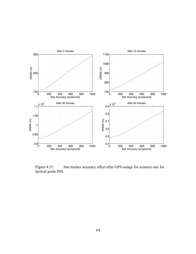
64

Figure 4.21: Star tracker accuracy effect after GPS outage for scenario one for tactical grade INS.

0 200 400 600 800 1000150

200

250


DR

MS

(m)

After 5 minutes

0 200 400 600 800 1000700

800

900

1000

1100

Star Accuracy (arcsecond)D

RM

S (m

)

After 10 minutes

0 200 400 600 800 10000.9

0.95

1

1.05

1.1 x 104


DR

MS

(m)

After 30 minutes

0 200 400 600 800 10004.4

4.5

4.6

4.7

4.8

4.9 x 104


DR

MS

(m)

After 60 minutes

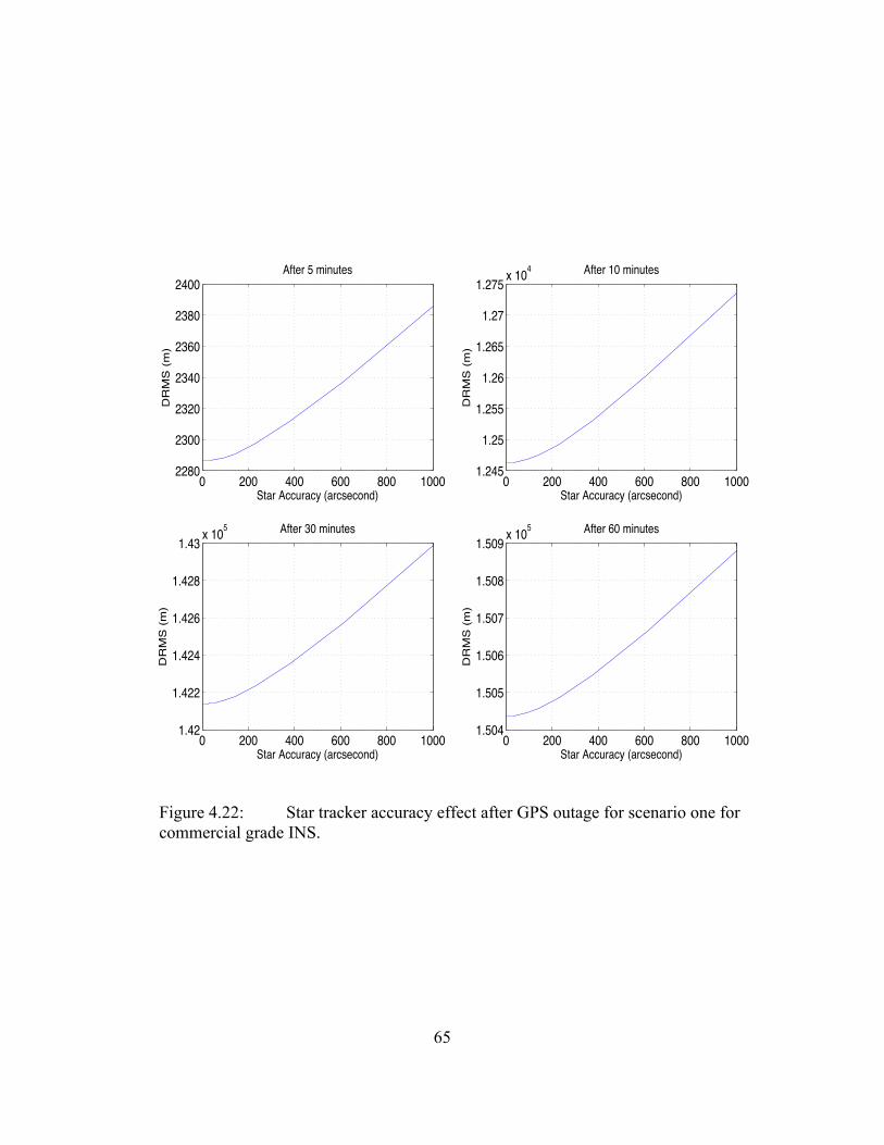
65

Figure 4.22: Star tracker accuracy effect after GPS outage for scenario one for commercial grade INS.

0 200 400 600 800 10002280

2300

2320

2340

2360

2380

2400


DR

MS

(m

)

After 5 minutes

0 200 400 600 800 10001.245

1.25

1.255

1.26

1.265

1.27

1.275 x 104


DR

MS

(m

)

After 10 minutes

0 200 400 600 800 10001.42

1.422

1.424

1.426

1.428

1.43 x 105


DR

MS

(m

)

After 30 minutes

0 200 400 600 800 10001.504

1.505

1.506

1.507

1.508

1.509 x 105


DR

MS

(m

)

After 60 minutes

66

V. Conclusion

his thesis presents a simulation for integrated star tracker and inertial sensors for

robust, self-contained, autonomous navigation. In this chapter, conclusions about

the research effort are presented and discussed. Also, areas for future research work are

addressed.

5.1 Conclusions

The goal of this research was to show the performance development in the

different types of INS when using a star tracker. The star tracker was used as an aiding

sensor to update and correct the orientation of the vehicle’s INS, and subsequently to

enhance the accuracy of position and velocity of the vehicle.

The research focused on two scenarios, these two scenarios were implemented

with three grades of INS commercial, tactical, and navigation. The first scenario was

about using the GPS for a small period in the beginning of the vehicle’s flight time, and

then it stops at a time where we assumed that the GPS is no longer available. In addition,

the star tracker and barometer were available in the first scenario for the total vehicle’s

flight time. The second scenario was similar to the first scenario, but instead of using a

star tracker, a barometer was used. These two scenarios were selected to show the

advantages of using the star tracker over the three different grades of INS.

After simulating the two scenarios with the three grades of INS, we had good

results that show the performance enhancement in the INS when a star tracker was used.

T

67

The star tracker was able to enhance the position, velocity, and tilts of all three grades of

INS. The enhancement degree changes form one INS grade to another depending on the

duration of the vehicle’s flight time and the accuracy of the inertial sensors used in the

three INS grades. The vehicle’s flight time in the simulation was 600 seconds, and the

GPS was used for the first 200 seconds.

For the commercial grade INS, the star tracker was able to correct the vehicle’s

position error covariance from 12×10!m to 3600m, which is a tremendous improvement

to the position. Also, it corrected the tilts covariance from 0.9rad to 5.8×10!!rad. The

star tracker showed a very good improvement to the commercial grade INS. Although the

final accuracy of 3600m is not very good.

For the tactical grade INS, the star tracker was able to correct the vehicle’s

position error covariance from 1000m to 300m, and it corrected the tilt covariance from

2×10!!rad to 5.1×10!!rad. The star tracker showed a very good improvement to the

tactical grade INS, on the 600 seconds time interval.

For the navigation grade INS, the simulation was carried out for two different

vehicle’s flight time. The first vehicle’s flight time was 600 seconds, and the star tracker

when used showed very little improvement to the navigation grade INS, that is because

the navigation grade INS uses a very good inertial sensors (i.e. gyroscopes and

accelerometers), and the vehicle’s flight time was small for the inertial sensors biases to

increase to a limit where the star tracker can make a difference. So, we increased the

vehicle’s flight time to 7200 seconds and made the GPS available for the first 200

seconds. In this situation, the position error covariance of the navigation grade INS

68

decreased from 6603m to 3370m, and the tilts covariance decreased from 5.9×10!!rad to

5.8×10!!rad when the star tracker was used.

In conclusion, the star tracker was able to improve the performance of the

commercial and tactical grades INS, for any duration of the vehicle’s flight time. Also,

the improvement in the performance of the navigation grade INS was not significant until

the vehicle’s flight time was more than approximately 1000 seconds.

5.2 Future Work Recommendations

This research has covered the basic simulation for using star tracker and the

inertial sensors, and the following points can improve the technique

• Study the relationship between stars locations and the vehicle’s location.

• Build a realistic star tracker measurement model.

• Test and analyze the star tracker measurement model by using different types of

Kalman filter.

The first point in my recommendations for future work is to deeply study the

relationship between the stars location and the navigating vehicle’s location. It includes

studying the stars locations in space and how can we benefit from knowing stars

locations, and how can we transform the stars locations using certain reference frames.

The second recommendation is to build a realistic star tracker measurement

model. This can be achieved if the first point is studied deeply. The measurement model

will include the Euler angles (i.e. roll, pitch, and yaw) and using the Euler angles as an

69

update measurement to the Kalman filter can improve the vehicle’s orientation and the

INS navigating parameters.

Using a realistic star tracker measurement model will enhance the reality of the

simulation results. Depending on the star tracker measurement model, different types of

Kalman filter could be used, such as an Extended Kalman Filter (EKF) or an Unscented

Kalman Filter (UKF). It would be useful to calculating the improvements to the

simulation results when using three filters.

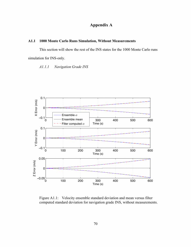
70

Appendix A

A1.1 1000 Monte Carlo Runs Simulation, Without Measurements

This section will show the rest of the INS states for the 1000 Monte Carlo runs

simulation for INS-only.

A1.1.1 Navigation Grade INS

Figure A1.1: Velocity ensemble standard deviation and mean versus filter computed standard deviation for navigation grade INS, without measurements.

0 100 200 300 400 500 600−0.1

0

0.1

Time (s)

X Er

ror (

m/s

)


0 100 200 300 400 500 600−0.1

0

0.1

Time (s)

Y Er

ror (

m/s

)

0 100 200 300 400 500 600−0.05

0

0.05

Time (s)

Z Er

ror (

m/s

)

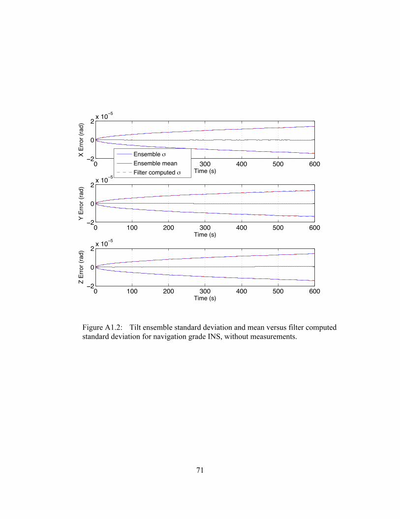
71

Figure A1.2: Tilt ensemble standard deviation and mean versus filter computed standard deviation for navigation grade INS, without measurements.

0 100 200 300 400 500 600−2

0

2x 10−5

Time (s)

X Er

ror (

rad)


0 100 200 300 400 500 600−2

0

2x 10−5

Time (s)

Y Er

ror (

rad)

0 100 200 300 400 500 600−2

0

2x 10−5

Time (s)

Z Er

ror (

rad)

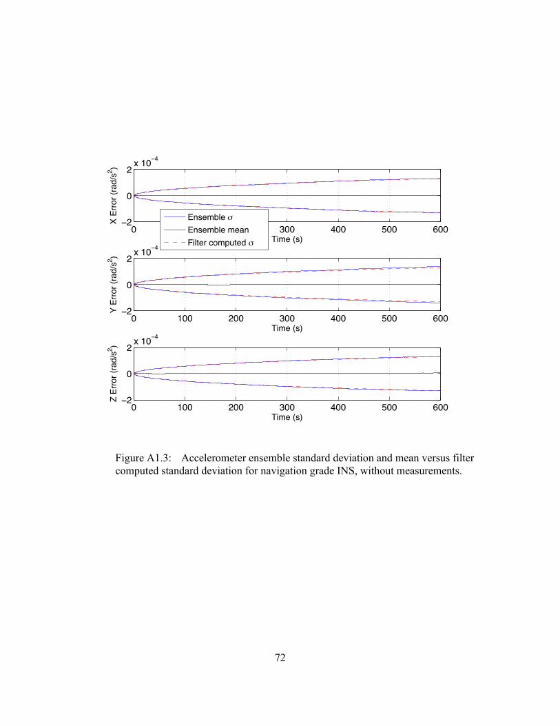
72

Figure A1.3: Accelerometer ensemble standard deviation and mean versus filter computed standard deviation for navigation grade INS, without measurements.

0 100 200 300 400 500 600−2

0

2x 10−4

Time (s)

X Er

ror (

rad/

s2 )


0 100 200 300 400 500 600−2

0

2x 10−4

Time (s)

Y Er

ror (

rad/

s2 )

0 100 200 300 400 500 600−2

0

2x 10−4

Time (s)

Z Er

ror (

rad/

s2 )

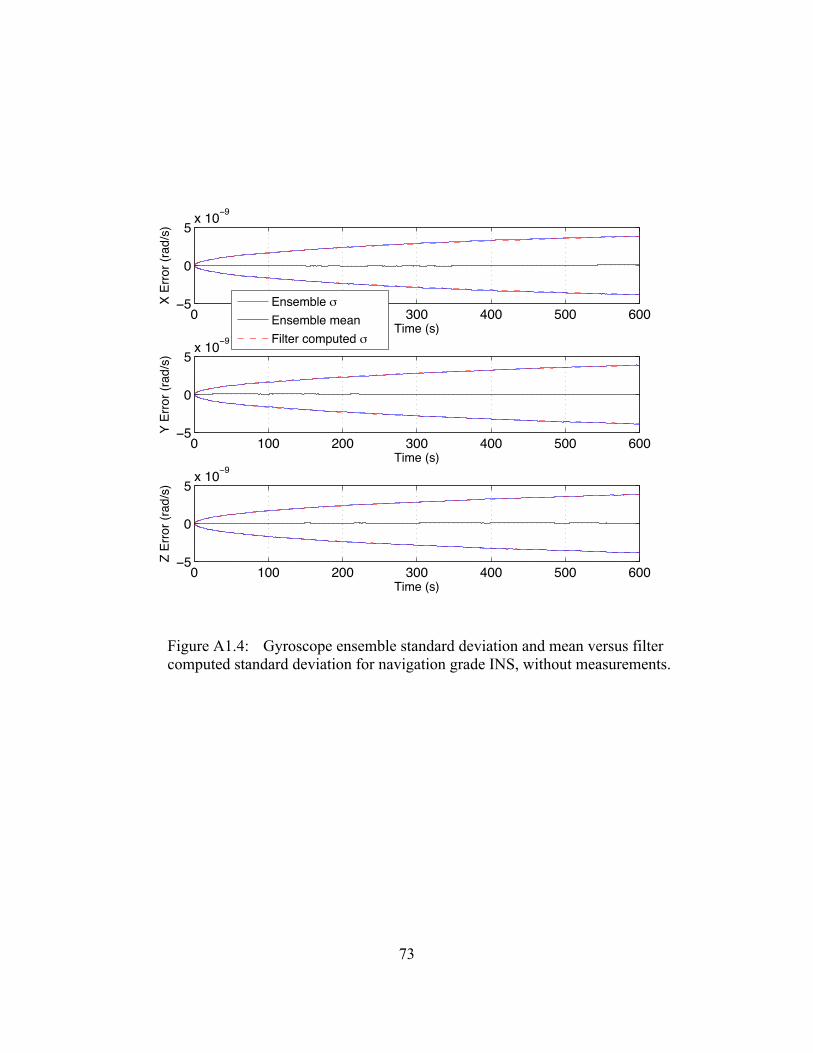
73

Figure A1.4: Gyroscope ensemble standard deviation and mean versus filter computed standard deviation for navigation grade INS, without measurements.

0 100 200 300 400 500 600−5

0

5x 10−9

Time (s)

X Er

ror (

rad/

s)


0 100 200 300 400 500 600−5

0

5x 10−9

Time (s)

Y Er

ror (

rad/

s)

0 100 200 300 400 500 600−5

0

5x 10−9

Time (s)

Z Er

ror (

rad/

s)

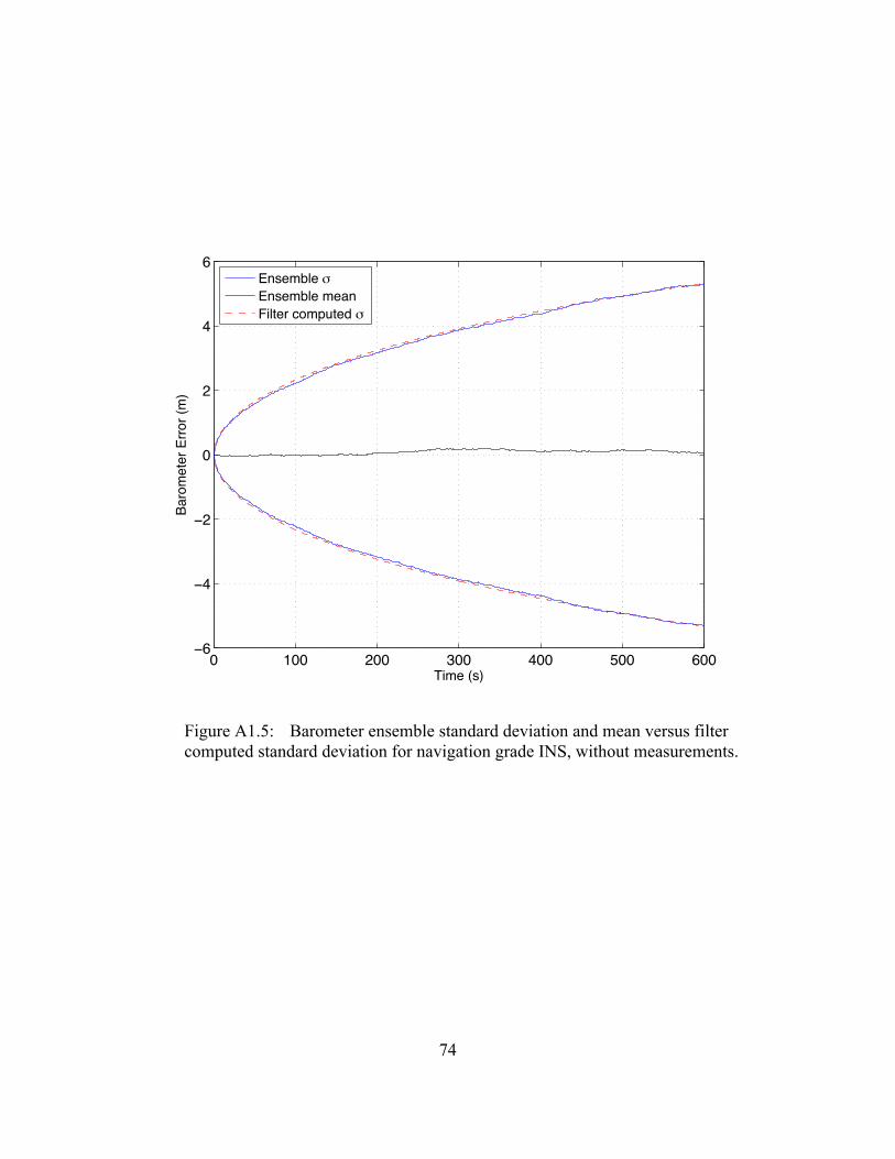
74

Figure A1.5: Barometer ensemble standard deviation and mean versus filter computed standard deviation for navigation grade INS, without measurements.

0 100 200 300 400 500 600−6

−4

−2

0

2

4

6

Time (s)

Baro

met

er E

rror (

m)


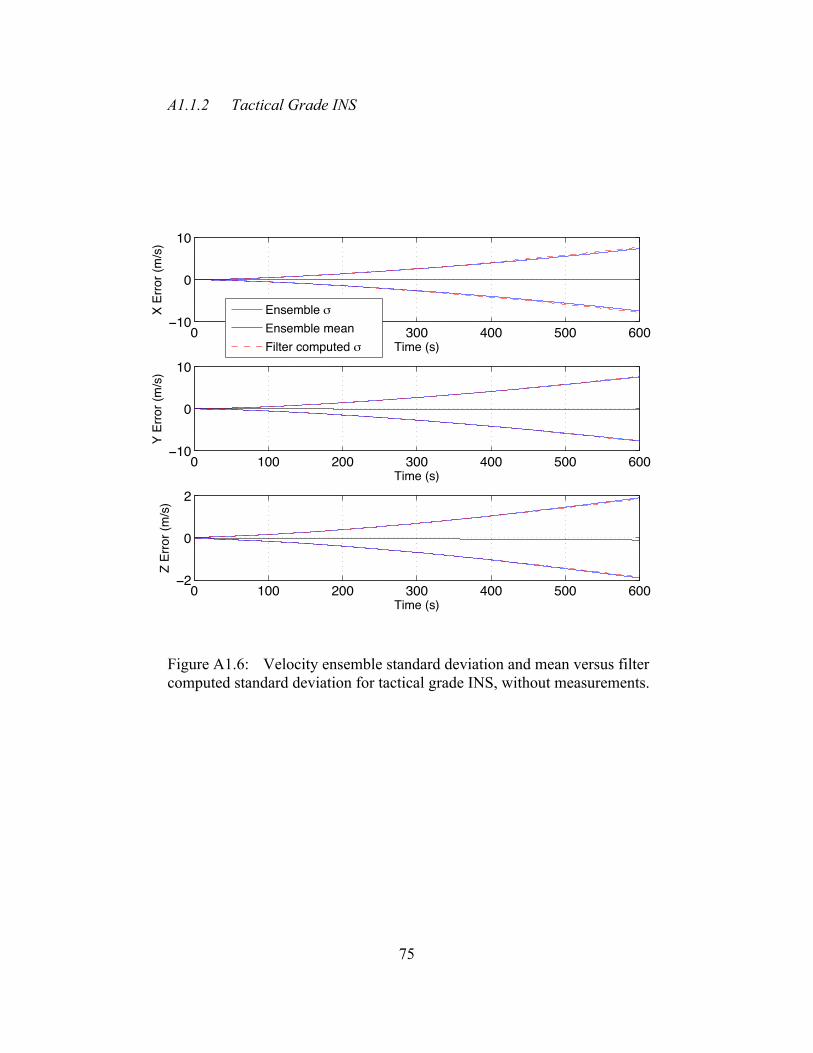
75

A1.1.2 Tactical Grade INS

Figure A1.6: Velocity ensemble standard deviation and mean versus filter computed standard deviation for tactical grade INS, without measurements.

0 100 200 300 400 500 600−10

0

10

Time (s)

X Er

ror (

m/s

)


0 100 200 300 400 500 600−10

0

10

Time (s)

Y Er

ror (

m/s

)

0 100 200 300 400 500 600−2

0

2

Time (s)

Z Er

ror (

m/s

)

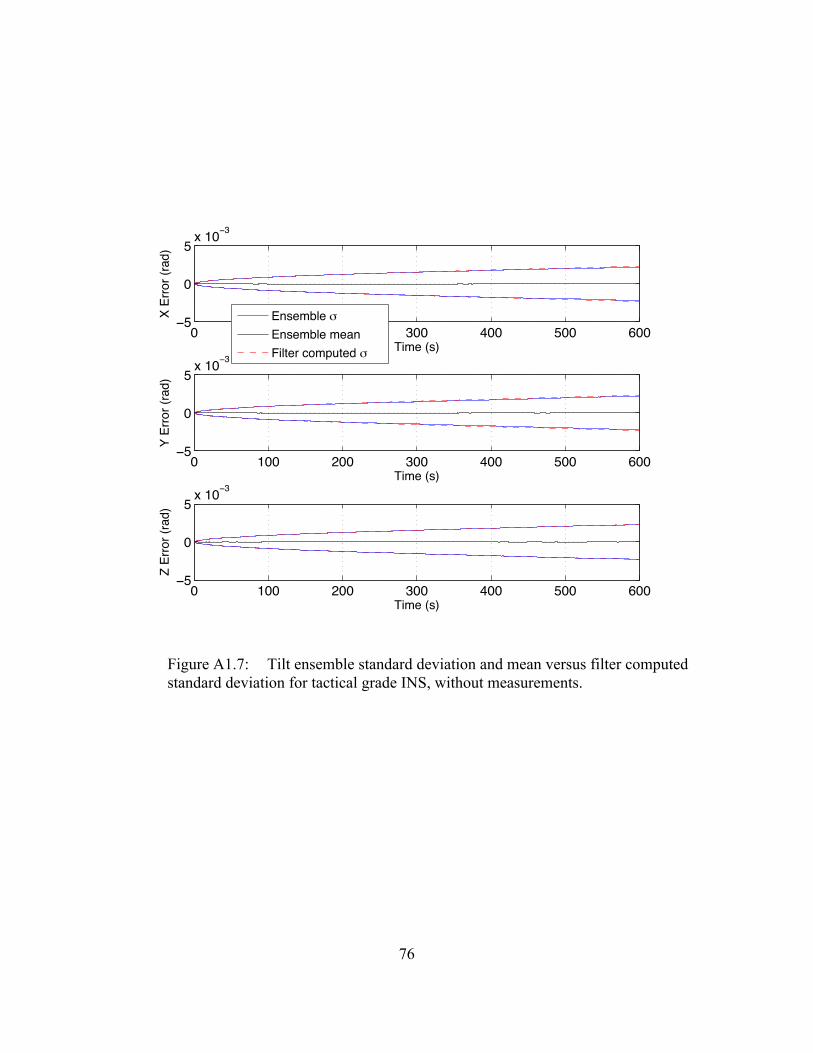
76

Figure A1.7: Tilt ensemble standard deviation and mean versus filter computed standard deviation for tactical grade INS, without measurements.

0 100 200 300 400 500 600−5

0

5x 10−3

Time (s)

X Er

ror (

rad)


0 100 200 300 400 500 600−5

0

5x 10−3

Time (s)

Y Er

ror (

rad)

0 100 200 300 400 500 600−5

0

5x 10−3

Time (s)

Z Er

ror (

rad)

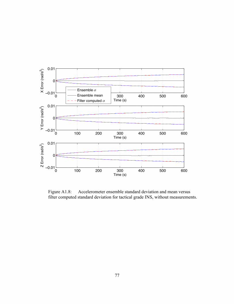
77

Figure A1.8: Accelerometer ensemble standard deviation and mean versus filter computed standard deviation for tactical grade INS, without measurements.

0 100 200 300 400 500 600−0.01

0

0.01

Time (s)

X Er

ror (

rad/

s2 )


0 100 200 300 400 500 600−0.01

0

0.01

Time (s)

Y Er

ror (

rad/

s2 )

0 100 200 300 400 500 600−0.01

0

0.01

Time (s)

Z Er

ror (

rad/

s2 )

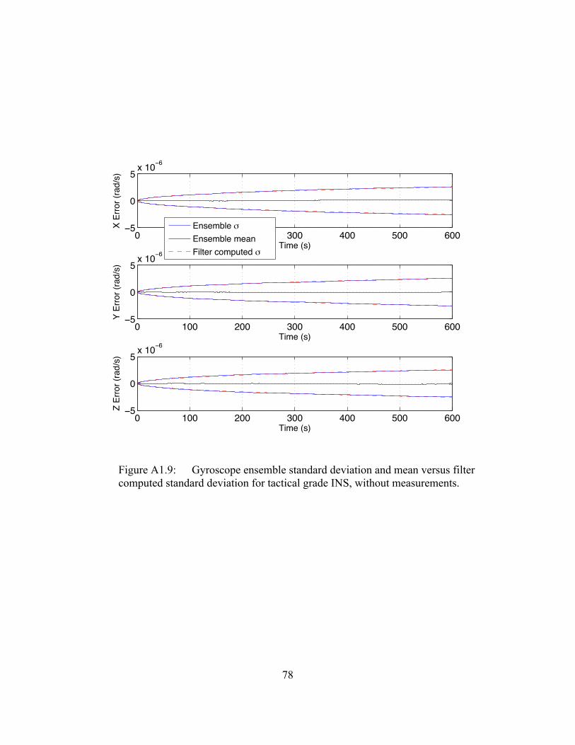
78

Figure A1.9: Gyroscope ensemble standard deviation and mean versus filter computed standard deviation for tactical grade INS, without measurements.

0 100 200 300 400 500 600−5

0

5x 10−6

Time (s)

X Er

ror (

rad/

s)


0 100 200 300 400 500 600−5

0

5x 10−6

Time (s)

Y Er

ror (

rad/

s)

0 100 200 300 400 500 600−5

0

5x 10−6

Time (s)

Z Er

ror (

rad/

s)

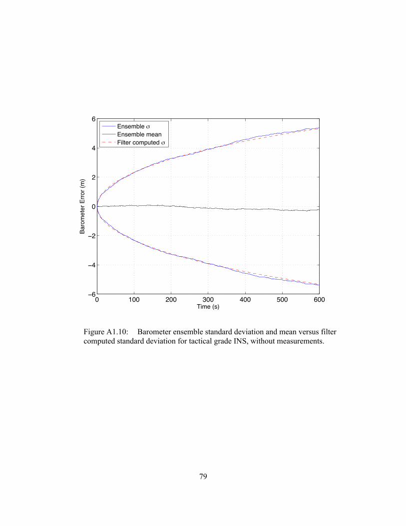
79

Figure A1.10: Barometer ensemble standard deviation and mean versus filter computed standard deviation for tactical grade INS, without measurements.

0 100 200 300 400 500 600−6

−4

−2

0

2

4

6

Time (s)

Baro

met

er E

rror (

m)


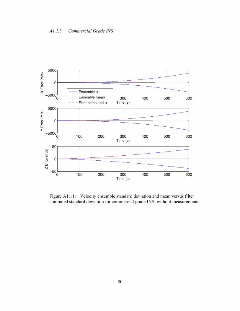
80

A1.1.3 Commercial Grade INS

Figure A1.11: Velocity ensemble standard deviation and mean versus filter computed standard deviation for commercial grade INS, without measurements.

0 100 200 300 400 500 600−5000

0

5000

Time (s)

X Er

ror (

m/s

)


0 100 200 300 400 500 600−5000

0

5000

Time (s)

Y Er

ror (

m/s

)

0 100 200 300 400 500 600−50

0

50

Time (s)

Z Er

ror (

m/s

)

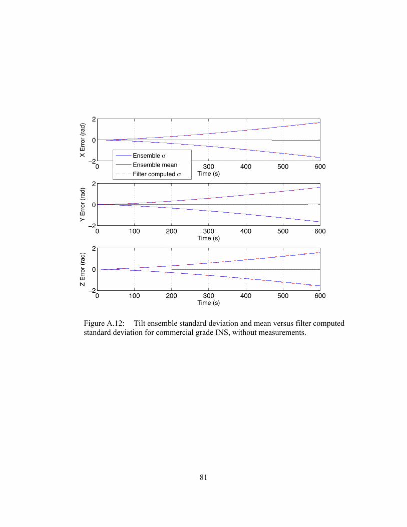
81

Figure A.12: Tilt ensemble standard deviation and mean versus filter computed standard deviation for commercial grade INS, without measurements.

0 100 200 300 400 500 600−2

0

2

Time (s)

X Er

ror (

rad)


0 100 200 300 400 500 600−2

0

2

Time (s)

Y Er

ror (

rad)

0 100 200 300 400 500 600−2

0

2

Time (s)

Z Er

ror (

rad)

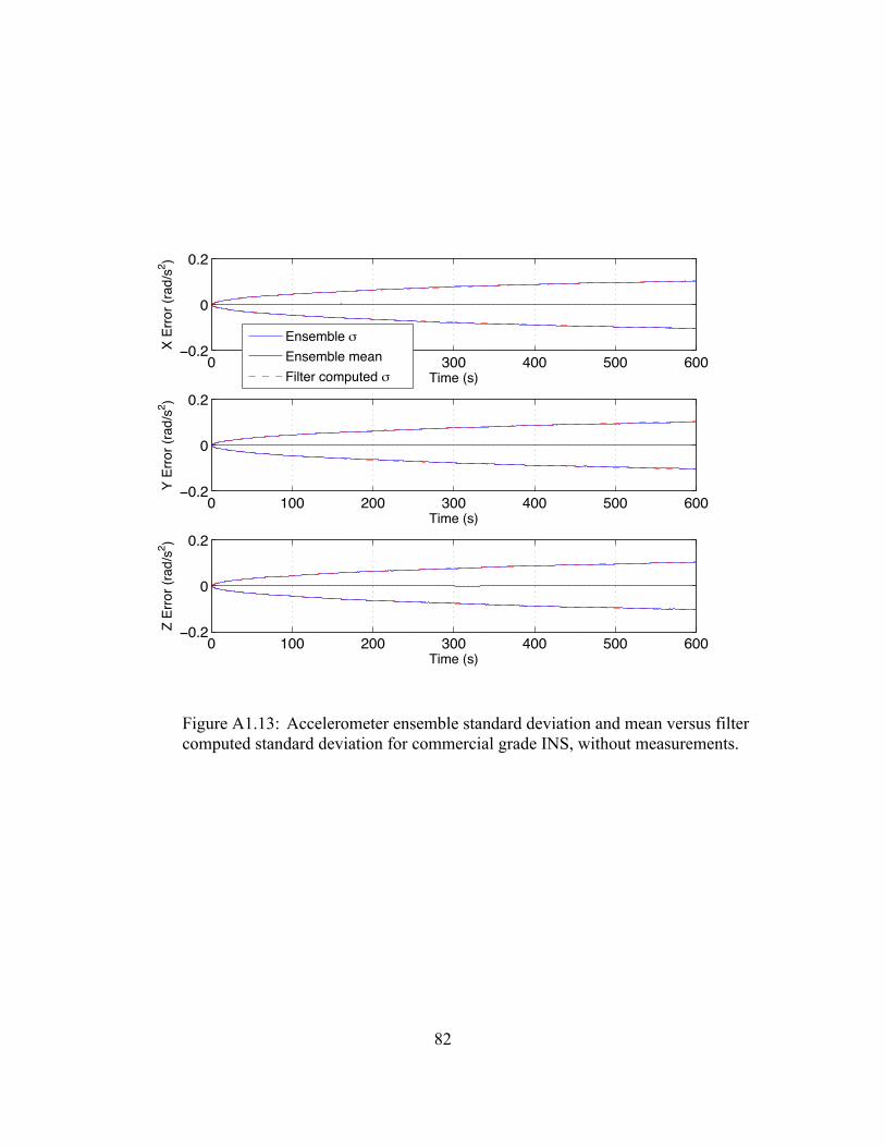
82

Figure A1.13: Accelerometer ensemble standard deviation and mean versus filter computed standard deviation for commercial grade INS, without measurements.

0 100 200 300 400 500 600−0.2

0

0.2

Time (s)

X Er

ror (

rad/

s2 )


0 100 200 300 400 500 600−0.2

0

0.2

Time (s)

Y Er

ror (

rad/

s2 )

0 100 200 300 400 500 600−0.2

0

0.2

Time (s)

Z Er

ror (

rad/

s2 )

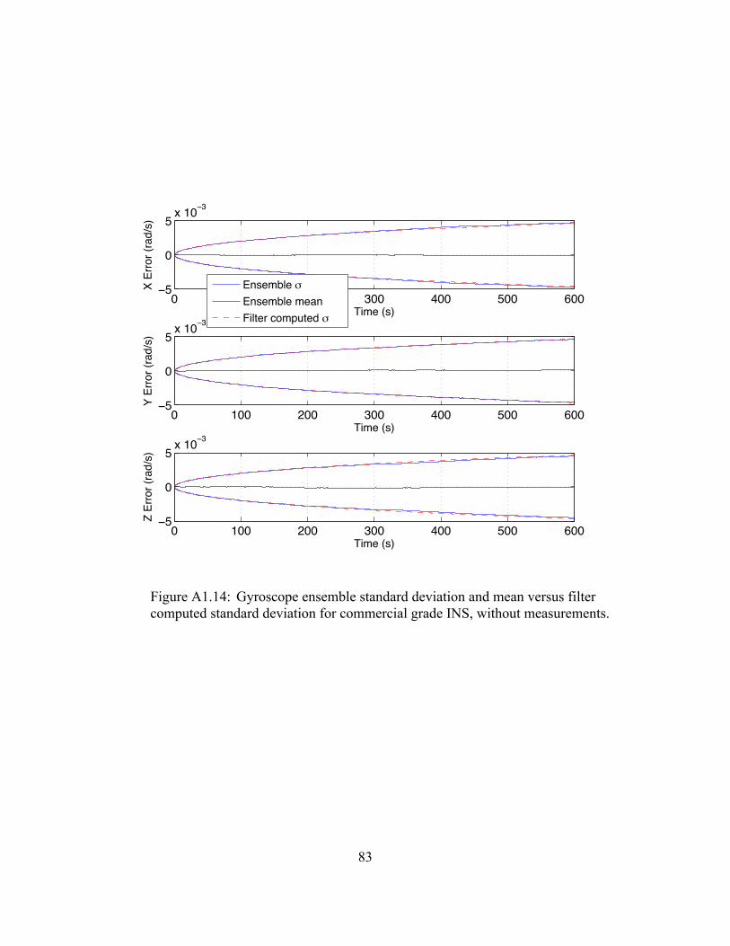
83

Figure A1.14: Gyroscope ensemble standard deviation and mean versus filter computed standard deviation for commercial grade INS, without measurements.

0 100 200 300 400 500 600−5

0

5x 10−3

Time (s)

X Er

ror (

rad/

s)


0 100 200 300 400 500 600−5

0

5x 10−3

Time (s)

Y Er

ror (

rad/

s)

0 100 200 300 400 500 600−5

0

5x 10−3

Time (s)

Z Er

ror (

rad/

s)

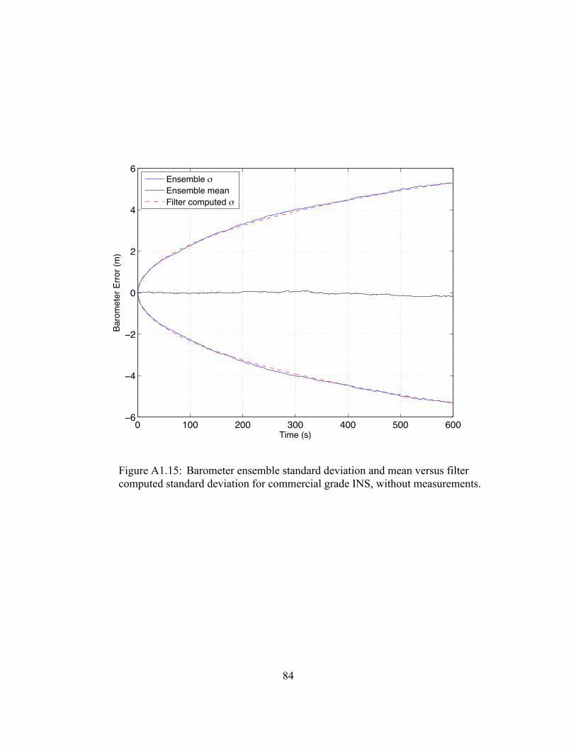
84

Figure A1.15: Barometer ensemble standard deviation and mean versus filter computed standard deviation for commercial grade INS, without measurements.

0 100 200 300 400 500 600−6

−4

−2

0

2

4

6

Time (s)

Baro

met

er E

rror (

m)


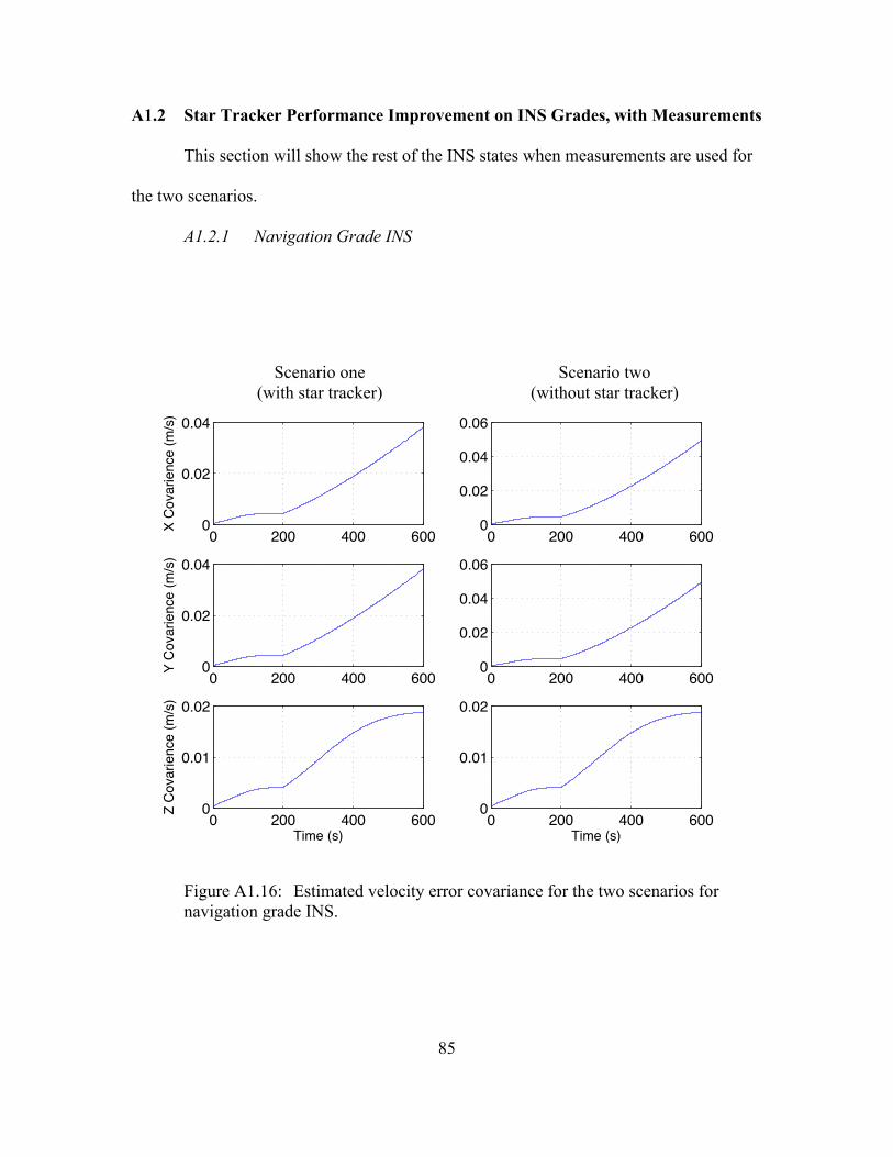
85

A1.2 Star Tracker Performance Improvement on INS Grades, with Measurements

This section will show the rest of the INS states when measurements are used for

the two scenarios.

A1.2.1 Navigation Grade INS

Figure A1.16: Estimated velocity error covariance for the two scenarios for navigation grade INS.

0 200 400 6000

0.02

0.04

X C

ovar

ienc

e (m

/s)

0 200 400 6000

0.02

0.04

Y C

ovar

ienc

e (m

/s)

0 200 400 6000

0.01

0.02

Time (s)

Z C

ovar

ienc

e (m

/s)

0 200 400 6000

0.02

0.04

0.06

0 200 400 6000

0.02

0.04

0.06

0 200 400 6000

0.01

0.02

Time (s)



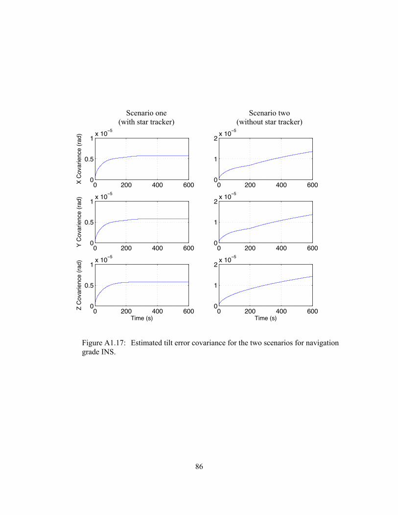
86

Figure A1.17: Estimated tilt error covariance for the two scenarios for navigation grade INS.

0 200 400 6000

0.5

1x 10−5

X C

ovar

ienc

e (ra

d)

0 200 400 6000

0.5

1x 10−5

Y C

ovar

ienc

e (ra

d)

0 200 400 6000

0.5

1x 10−5

Time (s)

Z C

ovar

ienc

e (ra

d)

0 200 400 6000

1

2x 10−5

0 200 400 6000

1

2x 10−5

0 200 400 6000

1

2x 10−5

Time (s)



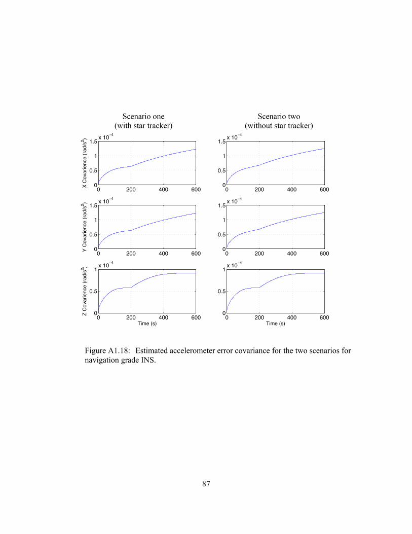
87

Figure A1.18: Estimated accelerometer error covariance for the two scenarios for navigation grade INS.

0 200 400 6000

0.5

1

1.5x 10−4

X C

ovar

ienc

e (ra

d/s2 )

0 200 400 6000

0.5

1

1.5x 10−4

Y C

ovar

ienc

e (ra

d/s2 )

0 200 400 6000

0.5

1x 10−4

Time (s)

Z C

ovar

ienc

e (ra

d/s2 )

0 200 400 6000

0.5

1

1.5x 10−4

0 200 400 6000

0.5

1

1.5x 10−4

0 200 400 6000

0.5

1x 10−4

Time (s)



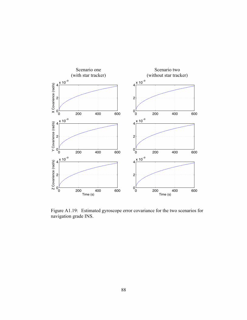
88

Figure A1.19: Estimated gyroscope error covariance for the two scenarios for navigation grade INS.

0 200 400 6000

2

4x 10−9

X C

ovar

ienc

e (ra

d/s)

0 200 400 6000

2

4x 10−9

Y C

ovar

ienc

e (ra

d/s)

0 200 400 6000

2

4x 10−9

Time (s)

Z C

ovar

ienc

e (ra

d/s)

0 200 400 6000

2

4x 10−9

0 200 400 6000

2

4x 10−9

0 200 400 6000

2

4x 10−9

Time (s)



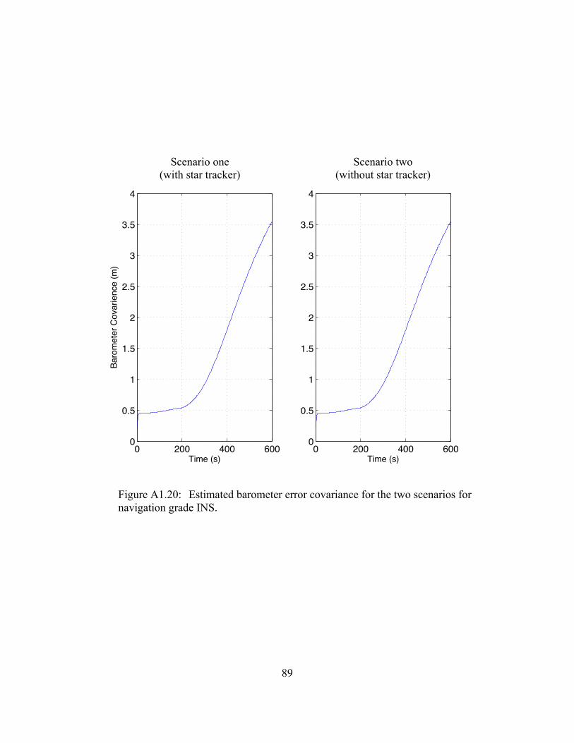
89

Figure A1.20: Estimated barometer error covariance for the two scenarios for navigation grade INS.

0 200 400 6000

0.5

1

1.5

2

2.5

3

3.5

4

Time (s)

Baro

met

er C

ovar

ienc

e (m

)

0 200 400 6000

0.5

1

1.5

2

2.5

3

3.5

4

Time (s)



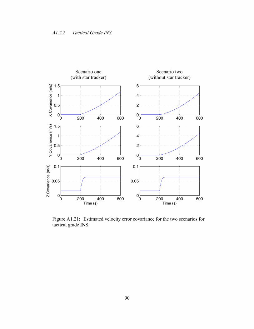
90

A1.2.2 Tactical Grade INS

Figure A1.21: Estimated velocity error covariance for the two scenarios for tactical grade INS.

0 200 400 6000

0.5

1

1.5

X C

ovar

ienc

e (m

/s)

0 200 400 6000

0.5

1

1.5

Y C

ovar

ienc

e (m

/s)

0 200 400 6000

0.05

0.1

Time (s)

Z C

ovar

ienc

e (m

/s)

0 200 400 6000

2

4

6

0 200 400 6000

2

4

6

0 200 400 6000

0.05

0.1

Time (s)



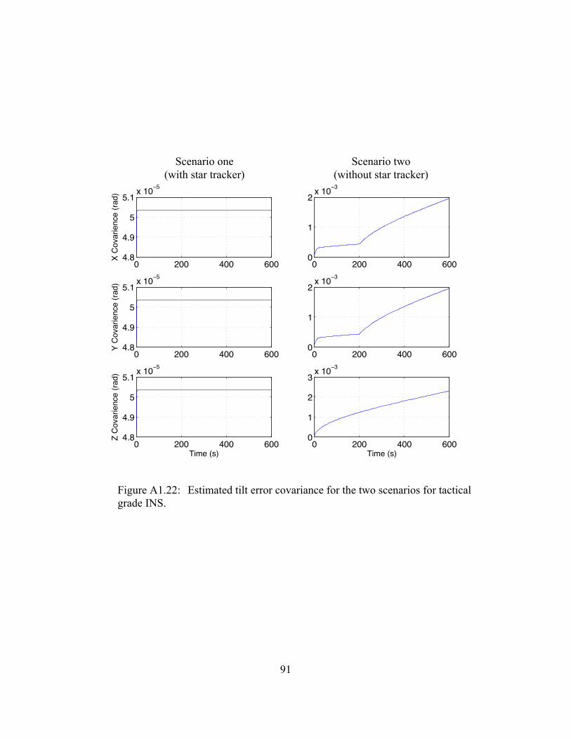
91

Figure A1.22: Estimated tilt error covariance for the two scenarios for tactical grade INS.

0 200 400 6004.8

4.9

5

5.1x 10−5

X C

ovar

ienc

e (ra

d)

0 200 400 6004.8

4.9

5

5.1x 10−5

Y C

ovar

ienc

e (ra

d)

0 200 400 6004.8

4.9

5

5.1x 10−5

Time (s)

Z C

ovar

ienc

e (ra

d)

0 200 400 6000

1

2x 10−3

0 200 400 6000

1

2x 10−3

0 200 400 6000

1

2

3x 10−3

Time (s)



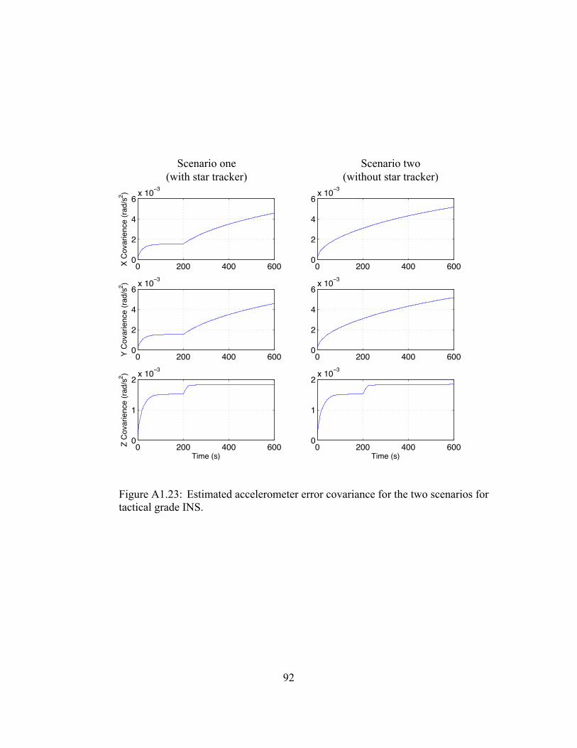
92

Figure A1.23: Estimated accelerometer error covariance for the two scenarios for tactical grade INS.

0 200 400 6000

2

4

6x 10−3

X C

ovar

ienc

e (ra

d/s2 )

0 200 400 6000

2

4

6x 10−3

Y C

ovar

ienc

e (ra

d/s2 )

0 200 400 6000

1

2x 10−3

Time (s)

Z C

ovar

ienc

e (ra

d/s2 )

0 200 400 6000

2

4

6x 10−3

0 200 400 6000

2

4

6x 10−3

0 200 400 6000

1

2x 10−3

Time (s)



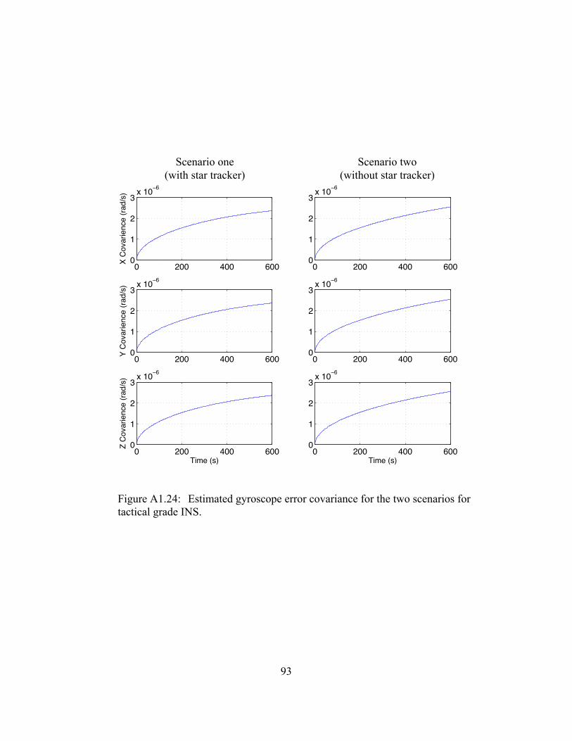
93

Figure A1.24: Estimated gyroscope error covariance for the two scenarios for tactical grade INS.

0 200 400 6000

1

2

3x 10−6

X C

ovar

ienc

e (ra

d/s)

0 200 400 6000

1

2

3x 10−6

Y C

ovar

ienc

e (ra

d/s)

0 200 400 6000

1

2

3x 10−6

Time (s)

Z C

ovar

ienc

e (ra

d/s)

0 200 400 6000

1

2

3x 10−6

0 200 400 6000

1

2

3x 10−6

0 200 400 6000

1

2

3x 10−6

Time (s)



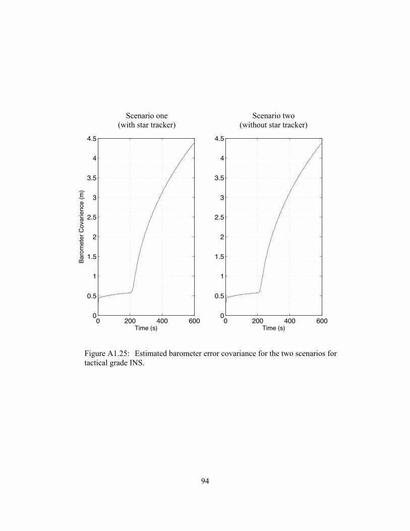
94

Figure A1.25: Estimated barometer error covariance for the two scenarios for tactical grade INS.

0 200 400 6000

0.5

1

1.5

2

2.5

3

3.5

4

4.5

Time (s)

Baro

met

er C

ovar

ienc

e (m

)

0 200 400 6000

0.5

1

1.5

2

2.5

3

3.5

4

4.5

Time (s)



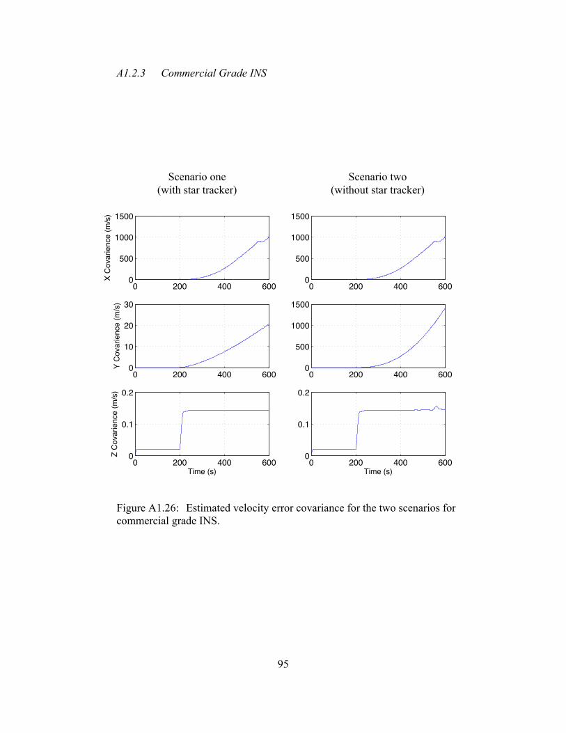
95

A1.2.3 Commercial Grade INS

Figure A1.26: Estimated velocity error covariance for the two scenarios for commercial grade INS.

0 200 400 6000

500

1000

1500

X C

ovar

ienc

e (m

/s)

0 200 400 6000

10

20

30

Y C

ovar

ienc

e (m

/s)

0 200 400 6000

0.1

0.2

Time (s)

Z C

ovar

ienc

e (m

/s)

0 200 400 6000

500

1000

1500

0 200 400 6000

500

1000

1500

0 200 400 6000

0.1

0.2

Time (s)



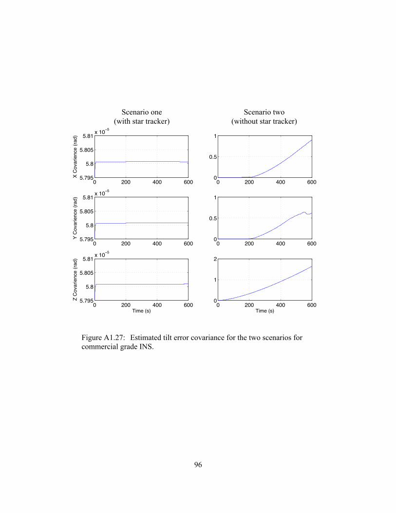
96

Figure A1.27: Estimated tilt error covariance for the two scenarios for commercial grade INS.

0 200 400 6005.795

5.8

5.805

5.81x 10−5

X C

ovar

ienc

e (ra

d)

0 200 400 6005.795

5.8

5.805

5.81x 10−5

Y C

ovar

ienc

e (ra

d)

0 200 400 6005.795

5.8

5.805

5.81x 10−5

Time (s)

Z C

ovar

ienc

e (ra

d)

0 200 400 6000

0.5

1

0 200 400 6000

0.5

1

0 200 400 6000

1

2

Time (s)



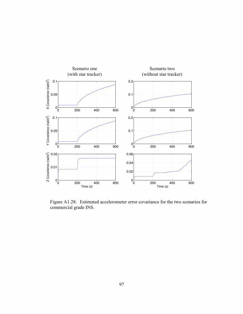
97

Figure A1.28: Estimated accelerometer error covariance for the two scenarios for commercial grade INS.

0 200 400 6000

0.05

0.1

X C

ovar

ienc

e (ra

d/s2 )

0 200 400 6000

0.05

0.1

Y C

ovar

ienc

e (ra

d/s2 )

0 200 400 6000

0.01

0.02

Time (s)

Z C

ovar

ienc

e (ra

d/s2 )

0 200 400 6000

0.1

0.2

0 200 400 6000

0.1

0.2

0 200 400 6000

0.02

0.04

0.06

Time (s)



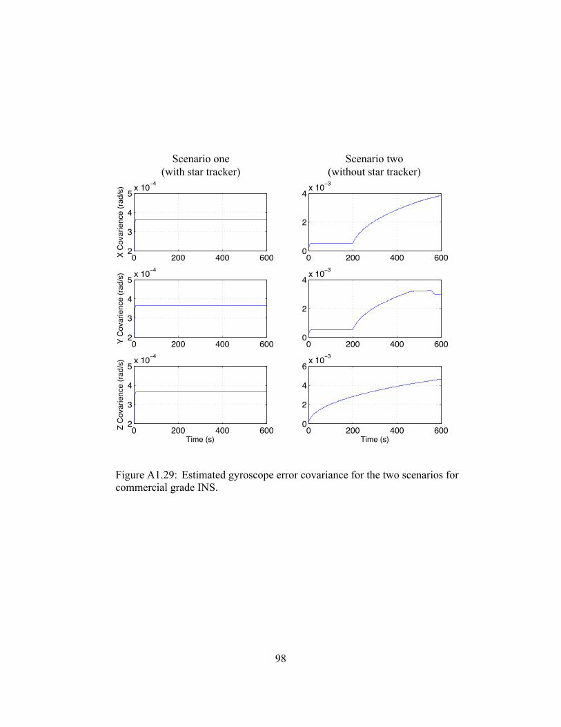
98

Figure A1.29: Estimated gyroscope error covariance for the two scenarios for commercial grade INS.

0 200 400 6002

3

4

5x 10−4

X C

ovar

ienc

e (ra

d/s)

0 200 400 6002

3

4

5x 10−4

Y C

ovar

ienc

e (ra

d/s)

0 200 400 6002

3

4

5x 10−4

Time (s)

Z C

ovar

ienc

e (ra

d/s)

0 200 400 6000

2

4x 10−3

0 200 400 6000

2

4x 10−3

0 200 400 6000

2

4

6x 10−3

Time (s)



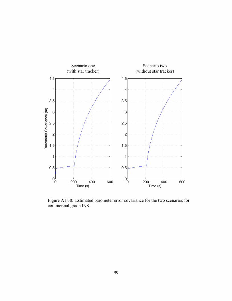
99

Figure A1.30: Estimated barometer error covariance for the two scenarios for commercial grade INS.

0 200 400 6000

0.5

1

1.5

2

2.5

3

3.5

4

4.5

Time (s)

Baro

met

er C

ovar

ienc

e (m

)

0 200 400 6000

0.5

1

1.5

2

2.5

3

3.5

4

4.5

Time (s)



100

Bibliography

1. Britting, Kenneth R. Inertial Navigation Systems Analysis. Wiley-Interscience, 1971.

2. D. H. Titterton and J. L.Weston, “ Strapdown Inertial Navigation Technology ”, second Edition.

3. F. Gul and Fang Jiancheng “Correction Technique for Velocity and Position Errors of Inertial Navigation System by Celestial Observations”, Emerging Technologies, 2005. Proceedings of the IEEE Symposium, on page(s): 7 pp. – 12.

4. Farid Gul and Fang Jiancheng “Alternate of GPS for Ballistic Vehicle Navigation”, Systems and Control in Aerospace and Astronautics, 2006. ISSCAA 2006. 1st International Symposium, On Page(s): 6 pp. – 24.

5. Hofmann-Wellenhof, “Global Positioning System, Theory and Practice”, Springer-Verlag New York, Inc; 2nd edition (Aug 7 2002).

6. S. J. Julier and J. K. Uhlmann, “ A new extension of the Kalman filter to nonlinear systems,” in Proc. AeroSense: 11th Int. Symp. Aerospace/Defence Sensing, Simulation and Controls, 1997, pp. 182-193.

7. Samaan, A. M., Mortari, D., & Junkins, L. J. (2008),”Compass Star Tracker for GPS-Like Applications”, IEEE Transactions On Aerospace And Electronic Systems. 44, 1629 – 1634.

8. National Imagery and Mapping Agency(NIMA) TR350.2,” World Geodetic System 198”,3rd edition, Departement of Defence, 3 january 2000.

9. Huffman, Kara M. (2006, May 26). “Designing star trackers to meet micro satellite requirements”. Retrieved from http://ssl.mit.edu/publications/theses/SM-2006-HuffmanKara.pdf

10. Weston John. Retrieved from http://www.globalspec.com/reference/26567/203279/chapter-11-strapdown-navigation-system-computation

11. Maybeck, Peter S. “Stochastic Models Estimation and Control”, Vol I. Academic Press, Inc., Orlando, Florida 32887, 1979.

12. M. Veth, “Fusion of imaging and inertial sensors for navigation,” Ph.D. dissertation, AFIT, Dayton, OH, 2006.

101

13. W.H. Steyn, M.J. Jacobs and P.J. Oosthuizen, “A High Performance Star Sensor System for Full Attitude Determination on a Microsatellite,” University of Stellenbosch, Stellenbosch 7600, South Africa.

14. Kyle Kauffman, “Radar based navigation in unknown terrain,” Ph.D. dissertation, AFIT, Dayton, OH, 2012.

15. Warden, John A., III. “Air Theory for the 21st Century”. Air and Space Expeditionary Operations, v4.0:108–119, 1994.

16. The Nobel Qur’an, Translation by Sahih International, Surat Al-'An`ām, verse 97.

17. Michaels, D., “ Ball Aerospace Star Tracker Achieves High Tracking Accuracy for a Moving Stars Field,” Aerospace Conference, 2005 IEEE , vol., no., pp.1,7, 5-12 March 2005.

102

REPORT DOCUMENTATION PAGE Form Approved OMB No. 074-0188

The public reporting burden for this collection of information is estimated to average 1 hour per response, including the time for reviewing instructions, searching existing data sources, gathering and maintaining the data needed, and completing and reviewing the collection of information. Send comments regarding this burden estimate or any other aspect of the collection of information, including suggestions for reducing this burden to Department of Defense, Washington Headquarters Services, Directorate for Information Operations and Reports (0704-0188), 1215 Jefferson Davis Highway, Suite 1204, Arlington, VA 22202-4302. Respondents should be aware that notwithstanding any other provision of law, no person shall be subject to an penalty for failing to comply with a collection of information if it does not display a currently valid OMB control number. PLEASE DO NOT RETURN YOUR FORM TO THE ABOVE ADDRESS. 1. REPORT DATE (DD-MM-YYYY)

18-09-2014 2. REPORT TYPE Master’s Thesis

3. DATES COVERED (From – To) Mar 2012 – Sep 2014

TITLE AND SUBTITLE Integration of a Star Tracker and Inertial Sensors Using an Attitude Update

5a. CONTRACT NUMBER

5b. GRANT NUMBER 5c. PROGRAM ELEMENT NUMBER

6. AUTHOR(S)

Humood Alkhaldi, Captain, RSAF

5d. PROJECT NUMBER

5e. TASK NUMBER

5f. WORK UNIT NUMBER

7. PERFORMING ORGANIZATION NAMES(S) AND ADDRESS(S) Air Force Institute of Technology Graduate School of Engineering and Management (AFIT/EN) 2950 Hobson Way, Building 640 WPAFB OH 45433-8865

8. PERFORMING ORGANIZATION REPORT NUMBER AFIT-ENG-T-14-S-16

9. SPONSORING/MONITORING AGENCY NAME(S) AND ADDRESS(ES) Intentionally left blank

10. SPONSOR/MONITOR’S ACRONYM(S)

11. SPONSOR/MONITOR’S REPORT NUMBER(S)

12. DISTRIBUTION/AVAILABILITY STATEMENT DISTRUBTION STATEMENT A. APPROVED FOR PUBLIC RELEASE; DISTRIBUTION UNLIMITED.

13. SUPPLEMENTARY NOTES This material is declared a work of the U.S. Government and is not subject to copyright protection in the United States.

14. ABSTRACT The Global Positioning System (GPS) is widely used in most of the military and civilian applications because of its precision navigation capability. Unfortunately, GPS is not available in all environments (e.g., indoors, under sea, under ground, or jamming environment). The motivation of this research is to address the limitations of GPS by using star trackers as an attitude update to an inertial navigation systems (INS). Commercial, tactical, and navigation grade INS are modeled and simulated with measurements from GPS, star tracker, and barometer. GPS measurements are used to update the INS position and velocity for a small duration in the beginning of the vehicle’s flight time. Star tracker and barometer measurements are used to update the INS attitude and altitude, respectively. This research uses a Linear Kalman Filter as a recursive estimation system, to estimate the INS errors (i.e. position, velocity, tilts, accelerometer bias, gyroscope bias, and barometer bias) using the three types of measurement updates. The simulation results show that the star tracker was able to improve the performance of the commercial and tactical grades INS, for any duration of the vehicle’s flight time. Also, the improvement in the performance of the navigation grade INS was not significant until the vehicle’s flight time was more than approximately 1000 seconds. Also, the research shows the performance impact on the three INS grades when using different star tracker accuracies. 15. SUBJECT TERMS navigation, image-aided navigation, inertial navigation, celestial navigation, autonomous navigation, global positioning, correspondence search, Kalman filter 16. SECURITY CLASSIFICATION OF: 17. LIMITATION

OF ABSTRACT

UU

18. NUMBER OF PAGES

115

19a. NAME OF RESPONSIBLE PERSON Dr. John F Raquet, AFIT/ENG

a. REPORT

U

b. ABSTRACT

U

c. THIS PAGE

U

19b. TELEPHONE NUMBER (Include area code) (937) 255-6565, ext 7264 ([email protected])

Standard Form 298 (Rev. 8-98) Prescribed by ANSI Std. Z39-18

Integration of a Star Tracker and Inertial Sensors Using ...

Documents

Transcript of Integration of a Star Tracker and Inertial Sensors Using ...