
Integrating Randomization and Discrimination for...
20
Integrating Randomization and Discrimination for Classifying Human-Object Interaction Activities Aditya Khosla, Bangpeng Yao and Li Fei-Fei 1 Introduction Psychologists have shown that the ability of humans to perform basic-level catego- rization (e.g. cars vs. dogs; kitchen vs. highway) develops well before their ability to perform subordinate-level categorization, or fine-grained visual categorization (e.g. distinguishing dog breeds such as Golden retrievers vs. Labradors) [18]. It is inter- esting to observe that computer vision research has followed a similar trajectory. Basic-level object and scene recognition has seen great progress [15, 21, 26, 31] while fine-grained categorization has received little attention. Unlike basic-level recognition, even humans might have difficulty with some of the fine-grained cate- gorization [32]. Thus, an automated visual system for this task could be valuable in many applications. Action recognition in still images can be regarded as a fine-grained classifi- cation problem [17] as the action classes only differ by human pose or type of human-object interactions. Unlike traditional object or scene recognition problems where different classes can be distinguished by different parts or coarse spatial lay- out [16, 21, 15], more detailed visual distinctions need to be explored for fine- grained image classification. The bounding boxes in Figure 1 demarcate the dis- tinguishing characteristics between closely related bird species, or different musical instruments or human poses that differentiate the different playing activities. Mod- els and algorithms designed for basic-level object or image categorization tasks are Aditya Khosla MIT, Cambridge, MA, USA, e-mail: [email protected] Bangpeng Yao Stanford University, Stanford, CA, USA, e-mail: [email protected] Li Fei-Fei Stanford University, Stanford, CA, USA, e-mail: [email protected] An early version of this chapter was presented in [37], and the code is available at http://vision.stanford.edu/discrim_rf/ 1
Transcript of Integrating Randomization and Discrimination for...

Integrating Randomization and Discriminationfor Classifying Human-Object InteractionActivities
Aditya Khosla, Bangpeng Yao and Li Fei-Fei
1 Introduction
Psychologists have shown that the ability of humans to perform basic-level catego-rization (e.g. cars vs. dogs; kitchen vs. highway) develops well before their ability toperform subordinate-level categorization, or fine-grained visual categorization (e.g.distinguishing dog breeds such as Golden retrievers vs. Labradors) [18]. It is inter-esting to observe that computer vision research has followed a similar trajectory.Basic-level object and scene recognition has seen great progress [15, 21, 26, 31]while fine-grained categorization has received little attention. Unlike basic-levelrecognition, even humans might have difficulty with some of the fine-grained cate-gorization [32]. Thus, an automated visual system for this task could be valuable inmany applications.
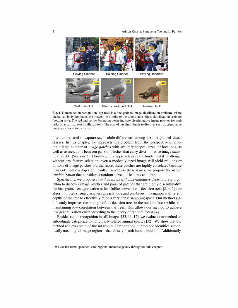
Action recognition in still images can be regarded as a fine-grained classifi-cation problem [17] as the action classes only differ by human pose or type ofhuman-object interactions. Unlike traditional object or scene recognition problemswhere different classes can be distinguished by different parts or coarse spatial lay-out [16, 21, 15], more detailed visual distinctions need to be explored for fine-grained image classification. The bounding boxes in Figure 1 demarcate the dis-tinguishing characteristics between closely related bird species, or different musicalinstruments or human poses that differentiate the different playing activities. Mod-els and algorithms designed for basic-level object or image categorization tasks are
Aditya KhoslaMIT, Cambridge, MA, USA, e-mail: [email protected]
Bangpeng YaoStanford University, Stanford, CA, USA, e-mail: [email protected]
Li Fei-FeiStanford University, Stanford, CA, USA, e-mail: [email protected]
An early version of this chapter was presented in [37], and the code is available athttp://vision.stanford.edu/discrim_rf/
1
2 Aditya Khosla, Bangpeng Yao and Li Fei-Fei
California Gull Glaucous-winged Gull Heerman Gull
Playing Clarinet Holding Clarinet Playing Recorder
Fig. 1 Human action recognition (top row) is a fine-grained image classification problem, wherethe human body dominates the image. It is similar to the subordinate object classification problem(bottom row). The red and yellow bounding boxes indicate discriminative image patches for bothtasks (manually drawn for illustration). The goal of our algorithm is to discover such discriminativeimage patches automatically.
often unprepared to capture such subtle differences among the fine-grained visualclasses. In this chapter, we approach this problem from the perspective of find-ing a large number of image patches with arbitrary shapes, sizes, or locations, aswell as associations between pairs of patches that carry discriminative image statis-tics [9, 33] (Section 3). However, this approach poses a fundamental challenge:without any feature selection, even a modestly sized image will yield millions orbillions of image patches. Furthermore, these patches are highly correlated becausemany of them overlap significantly. To address these issues, we propose the use ofrandomization that considers a random subset of features at a time.
Specifically, we propose a random forest with discriminative decision trees algo-rithm to discover image patches and pairs of patches that are highly discriminativefor fine-grained categorization tasks. Unlike conventional decision trees [8, 4, 2], ouralgorithm uses strong classifiers at each node and combines information at differentdepths of the tree to effectively mine a very dense sampling space. Our method sig-nificantly improves the strength of the decision trees in the random forest while stillmaintaining low correlation between the trees. This allows our method to achievelow generalization error according to the theory of random forest [4].
Besides action recognition in still images [33, 11, 12], we evaluate our method onsubordinate categorization of closely related animal species [32]. We show that ourmethod achieves state-of-the-art results. Furthermore, our method identifies seman-tically meaningful image regions1 that closely match human intuition. Additionally,
1 We use the terms ‘patches’ and ‘regions’ interchangeably throughout this chapter.
Title Suppressed Due to Excessive Length 3
our method tends to automatically generate a coarse-to-fine structure of discrimina-tive image patches, which parallels the human visual system [5].
The remaining part of this chapter is organized as follows: Section 2 discussesrelated work. Section 3 describes our dense feature space and Section 4 describesour algorithm for mining this space. Experimental results are discussed in Section 5,and Section 6 summarizes this chapter.
2 Related work
Image classification has been studied for many years. Most of the existing workfocuses on basic-level categorization such as objects [14, 2, 15] or scenes [26, 13,21]. In this chapter we focus on two tasks of fine-grained image classification: (1)identifying human-object interaction activities in still images [35, 36, 39, 34], andsubordinate-level categorization of animal species [17, 3, 20, 38], which requires anapproach that captures the fine and detailed information in images.
In this chapter, we explore a dense feature representation to distinguish fine-grained image classes. “Grouplet” features [33] have shown the advantage of densefeatures in classifying human activities. Instead of using the generative local featuresas in Grouplet, here we consider a richer feature space in a discriminative settingwhere both local and global visual information are fused together. Inspired by [9,33], our approach also considers pairwise interactions between image regions.
We use a random forest framework to identify discriminative image regions. Ran-dom forests have been used successfully in many vision tasks such as object de-tection [2], segmentation [27] and codebook learning [24]. Inspired from [28], wecombine discriminative training and randomization to obtain an effective classifierwith good generalizability. Our method differs from [28] in that for each tree node,we train an SVM classifier from one of the randomly sampled image regions, in-stead of using AdaBoost to combine weak features from a fixed set of regions. Thisallows us to explore an extremely large feature set efficiently.
A classical image classification framework [31] is Feature Extraction→ Coding→ Pooling→ Concatenating. Feature extraction [23] and better coding and poolingmethods [31] have been extensively studied for object recognition. In this work,we use discriminative feature mining and randomization to propose a new featureconcatenating approach, and demonstrate its effectiveness on fine-grained imagecategorization tasks.
3 Dense sampling space
Our algorithm aims to identify fine image statistics that are useful for fine-grainedcategorization. For example, in order to classify whether a human is playing a guitaror holding a guitar without playing it, we want to use the image patches below the
4 Aditya Khosla, Bangpeng Yao and Li Fei-Fei
(a) (b)
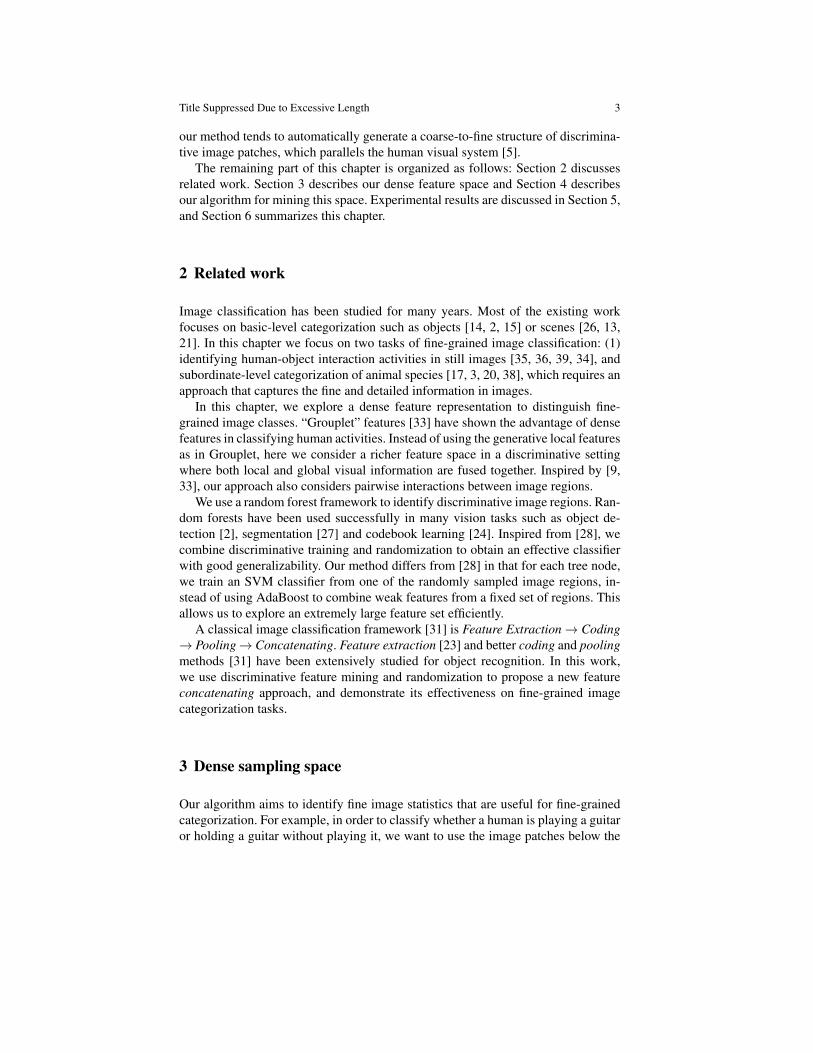
Fig. 2 Illustration of the proposed dense sampling space. (a) We densely sample rectangular im-age patches with varying widths and heights. The regions are closely located and have significantoverlaps. The red × denote the centers of the patches, and the arrows indicate the increment ofthe patch width or height. (b) Illustration of some image patches that may be discriminative for“playing-guitar”. All those patches can be sampled from our dense sampling space.
human face that are closely related to the human-guitar interaction (Figure 2(b)). Analgorithm that can reliably locate such regions is expected to achieve high classifica-tion accuracy. We achieve this goal by searching over rectangular image patches ofarbitrary width, height, and image location. We refer to this extensive set of imageregions as the dense sampling space, as shown in Figure 2(a). This figure has beensimplified for visual clarity, and the actual density of regions considered in our algo-rithm is significantly higher. We note that the regions considered by spatial pyramidmatching [21] is a very small subset lying along the diagonal of the height-widthplane that we consider. Further, to capture more discriminative distinctions, we alsoconsider interactions between pairs of arbitrary patches. The pairwise interactionsare modeled by applying concatenation, absolute of difference, or intersection be-tween the feature representations of two image patches.
However, the dense sampling space is very huge. Sampling image patches of size50×50 in a 400×400 image every four pixels leads to thousands of patches. Thisincreases many-folds when considering regions with arbitrary widths and heights.Further considering pairwise interactions of image patches will effectively lead totrillions of features for each image. In addition, there is much noise and redundancyin this feature set. On the one hand, many image patches are not discriminativefor distinguishing different image classes. On the other hand, the image patchesare highly overlapped in the dense sampling space, which introduces significantredundancy among these features. Therefore, it is challenging to explore this high-dimensional, noisy, and redundant feature space. In this work, we address this issueusing randomization.
Title Suppressed Due to Excessive Length 5
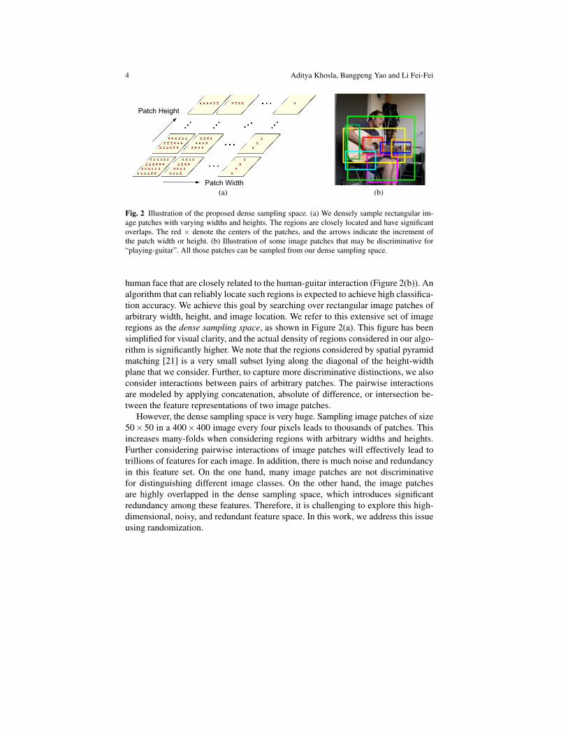
foreach tree t do- Sample a random set of training examples D ;- SplitNode(D);if needs to split then
i. Randomly sample the candidate (pairs of) image regions (Section 4.2);ii. Select the best region to split D into two sets D1 and D2 (Section 4.3);iii. Go to SplitNode(D1) and SplitNode(D2).
elseReturn Pt(c) for the current leaf node.
endend
Algorithm 1: Overview of the process of growing decision trees in the randomforest framework.
4 Discriminative random forest
In order to explore the dense sampling feature space for fine-grained visual cate-gorization, we combine two concepts: (1) Discriminative training to extract the in-formation in the image patches effectively; (2) Randomization to explore the densefeature space efficiently. Specifically, we adopt a random forest [4] framework whereeach tree node is a discriminative classifier that is trained on one or a pair of imagepatches. In our setting, the discriminative training and randomization can benefitfrom each other. We summarize the advantages of our method below:
• The random forest framework allows us to consider a subset of the image regionsat a time, which allows us to explore the dense sampling space efficiently in aprincipled way.
• Random forest selects a best image patch in each node, and therefore it can re-move the noise-prone image patches and reduce redundancy in the feature set.
• By using discriminative classifiers to train the tree nodes, our random forest hasmuch stronger decision trees. Further, because of the large number of possibleimage regions, it is likely that different decision trees will use different imageregions, which reduces the correlation between decision trees. Therefore, ourmethod is likely to achieve low generalization error (Section 4.4) compared withthe traditional random forest [4] which uses weak classifiers in the tree nodes.
An overview of the random forest framework we use is shown in Algorithm 1. Inthe following sections, we first describe this framework (Section 4.1). Then we elab-orate on our feature sampling (Section 4.2) and split learning (Section 4.3) strategiesin detail, and describe the generalization theory [4] of random forest which guaran-tees the effectiveness of our algorithm (Section 4.4).
6 Aditya Khosla, Bangpeng Yao and Li Fei-Fei
Weak
classifier
Leaf
(a) Conventional random decision tree.
Strong
classifier
Leaf
(b) The proposed discriminative decision tree.
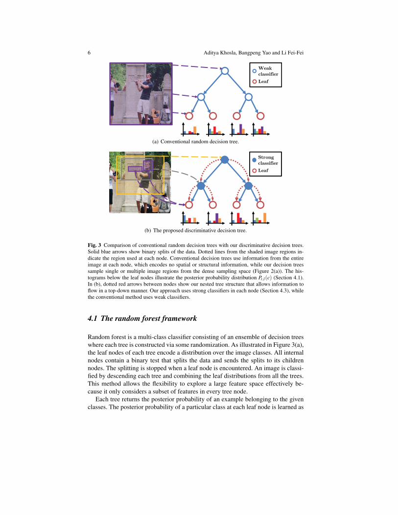
Fig. 3 Comparison of conventional random decision trees with our discriminative decision trees.Solid blue arrows show binary splits of the data. Dotted lines from the shaded image regions in-dicate the region used at each node. Conventional decision trees use information from the entireimage at each node, which encodes no spatial or structural information, while our decision treessample single or multiple image regions from the dense sampling space (Figure 2(a)). The his-tograms below the leaf nodes illustrate the posterior probability distribution Pt,l(c) (Section 4.1).In (b), dotted red arrows between nodes show our nested tree structure that allows information toflow in a top-down manner. Our approach uses strong classifiers in each node (Section 4.3), whilethe conventional method uses weak classifiers.
4.1 The random forest framework
Random forest is a multi-class classifier consisting of an ensemble of decision treeswhere each tree is constructed via some randomization. As illustrated in Figure 3(a),the leaf nodes of each tree encode a distribution over the image classes. All internalnodes contain a binary test that splits the data and sends the splits to its childrennodes. The splitting is stopped when a leaf node is encountered. An image is classi-fied by descending each tree and combining the leaf distributions from all the trees.This method allows the flexibility to explore a large feature space effectively be-cause it only considers a subset of features in every tree node.
Each tree returns the posterior probability of an example belonging to the givenclasses. The posterior probability of a particular class at each leaf node is learned as

Title Suppressed Due to Excessive Length 7
the proportion of the training images belonging to that class at the given leaf node.The posterior probability of class c at leaf l of tree t is denoted as Pt,l(c). Thus, a testimage can be classified by averaging the posterior probability from the leaf node ofeach tree:
c∗ = argmaxc
1T
T
∑t=1
Pt,lt (c), (1)
where c∗ is the predicted class label, T is the total number of trees, and lt is the leafnode that the image falls into.
In the following sections, we describe the process of obtaining Pt,l(c) using ouralgorithm. Readers can refer to previous works [4, 2, 27] for more details of theconventional decision tree learning procedure.
4.2 Sampling the dense feature space
As shown in Figure 3(b), each internal node in our decision tree corresponds to asingle or a pair of rectangular image regions that are sampled from the dense sam-pling space (Section 3), where the regions can have many possible widths, heights,and image locations. In order to sample a candidate image region, we first normalizeall images to unit width and height, and then randomly sample (x1,y1) and (x2,y2)from a uniform distribution U([0,1]). These coordinates specify two diagonally op-posite vertices of a rectangular region. Such regions could correspond to small areasof the image (e.g. the purple bounding boxes in Figure 3(b)) or even the completeimage. This allows our method to capture both global and local information in theimage.
In our approach, each sampled image region is represented by a histogram ofvisual descriptors. For a pair of regions, the feature representation is formed by ap-plying histogram operations (e.g. concatenation, intersection, etc.) to the histogramsobtained from both regions. Furthermore, the features are augmented with the deci-sion value wTf (described in Section 4.3) of this image from its parent node (indi-cated by the dashed red lines in Figure 3(b)). Therefore, our feature representationcombines the information of all upstream tree nodes that the corresponding imagehas descended from. We refer to this idea as “nesting”. Using feature sampling andnesting, we obtain a candidate set of features, f ∈ Rn, corresponding to a candidateimage region of the current node.
Implementation details. Our method is flexible to use many different visualdescriptors. In this work, we densely extract SIFT [23] descriptors on each imagewith a spacing of four pixels. The scales of the grids to extract descriptors are 8, 12,16, 24, and 30. Using k-means clustering, we construct a vocabulary of codewords2.Then, we use Locality-constrained Linear Coding [31] to assign the descriptors to
2 A dictionary size of 1024, 256, 256 is used for PASCAL action [11, 12], PPMI [33], and Caltech-UCSD Birds [32] datasets respectively.
8 Aditya Khosla, Bangpeng Yao and Li Fei-Fei
codewords. A bag-of-words histogram representation is used if the area of the patchis smaller than 0.2, while a 2-level or 3-level spatial pyramid is used if the area isbetween 0.2 and 0.8 or larger than 0.8 respectively. Note that all parameter here areempirically chose. Using other similar parameters will lead to very similar results.
During sampling (step i of Algorithm 1), we consider four settings of imagepatches: a single image patch and three types of pairwise interactions (concatena-tion, intersection, and absolute of difference of the two histograms). We sample25 and 50 image regions (or pairs of regions) in the root node and the first levelnodes respectively, and sample 100 regions (or pairs of regions) in all other nodes.Sampling a smaller number of image patches in the root can reduce the correlationbetween the resulting trees.
4.3 Learning the splits
In this section, we describe the process of learning the binary splits of the data usingSVM (step ii in Algorithm 1). This is achieved in two steps: (1) Randomly assigningall examples from each class to a binary label; (2) Using SVM to learn a binary splitof the data.
Assume that we have C classes of images at a given node. We uniformly sampleC binary variables, b, and assign all examples of a particular class ci a class label ofbi. As each node performs a binary split of the data, this allows us to learn a simplebinary SVM at each node. This improves the scalability of our method to a largenumber of classes and results in well-balanced trees. Using the feature representa-tion f of an image region (or pairs of regions) as described in Section 4.2, we find abinary split of the data: {
wTf≤ 0,go to left childotherwise,go to right child
where w is the set of weights learned from a linear SVM.We evaluate each binary split that corresponds to an image region or pairs of
regions with the information gain criteria [2], which is computed from the com-plete training images that fall at the current tree node. The splits that maximize theinformation gain are selected and the splitting process (step iii in Algorithm 1) isrepeated with the new splits of the data. The tree splitting stops if a pre-specifiedmaximum tree depth has been reached, or the information gain of the current nodeis larger than a threshold, or the number of samples in the current node is small.
Title Suppressed Due to Excessive Length 9
4.4 Generalization error of random forests
In [4], it has been shown that an upper bound for the generalization error of a randomforest is given by
ρ(1− s2)/s2, (2)
where s is the strength of the decision trees in the forest, and ρ is the correlationbetween the trees. Therefore, the generalization error of a random forest can bereduced by making the decision trees stronger or reducing the correlation betweenthe trees.
In our approach, we learn discriminative SVM classifiers for the tree nodes.Therefore, compared to the traditional random forests where the tree nodes are weakclassifiers of randomly generated feature weights [2], our decision trees are muchstronger. Furthermore, since we are considering an extremely dense feature space,each decision tree only considers a relatively small subset of image patches. Thismeans there is little correlation between the trees. Therefore, our random forestwith discriminative decision trees algorithm can achieve very good performance onfine-grained image classification, where exploring fine image statistics discrimina-tively is important. In Section 5.5, we show the strength and correlation of differentsettings of random forests with respect to the number of decision trees, which jus-tifies the above arguments. Please refer to [4] for details about how to compute thestrength and correlation values for a random forest.
5 Experiments
In this section, we first evaluate our algorithm on two fine-grained image datasets:actions of people-playing-musical-instrument (PPMI) [33] (Section 5.1) and a sub-ordinate object categorization dataset of 200 bird species [32] (Section 5.2). Ex-perimental results show that our algorithm outperforms state-of-the-art methods onthese datasets. Further, we use the proposed method to participate the action classi-fication competition of the PASCAL VOC challenge, and obtain the winning awardin both 2011 [11] and 2012 [12]. Detailed results and analysis are shown in Sec-tion 5.3 and Section 5.4. Finally, we evaluate the strength and correlation of thedecision trees in our method, and compare the result with the other settings of ran-dom forests to show why our method can lead to better classification performance(Section 5.5).

10 Aditya Khosla, Bangpeng Yao and Li Fei-Fei
Method BoW Grouplet [33] SPM [21] LLC [31] Ours
mAP (%) 22.7 36.7 39.1 41.8 47.0
Table 1 Mean Average Precision (% mAP) on the 24-class classification problem of the PPMIdataset. The best result is highlighted with bold fonts.
5.1 People-Playing-Musical-Instruments (PPMI)
The people-playing-musical-instrument (PPMI) data set is introduced in [33]. Thisdata set puts emphasis on understanding subtle interactions between humans andobjects. Here we use a full version of the dataset which contains twelve musicalinstruments; for each instrument there are images of people playing the instrumentand holding the instrument but not playing it. We evaluate the performance of ourmethod with 100 decision trees on the 24-class classification problem. We compareour method with many previous results3, including bag of words, grouplet [33], spa-tial pyramid matching (SPM) [21], locality-constrained linear coding (LLC) [31].The grouplet method uses one SIFT scale, while all the other methods use multipleSIFT scales described in Section 4.2. Table 1 shows that we significantly outperformthe a various of previous approaches.
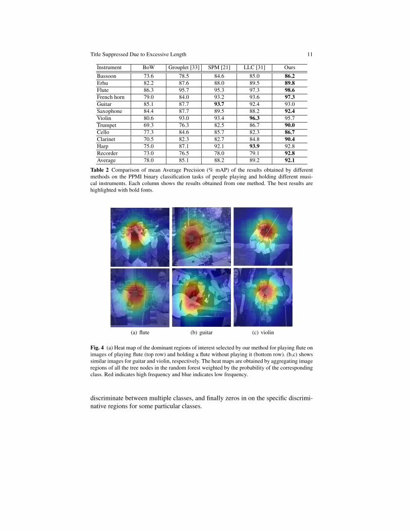
Table 2 shows the result of our method on the 12 binary classification tasks whereeach task involves distinguishing the activities of playing and not playing for thesame instrument. Despite a high baseline of 89.2% mAP, our method outperformsby 2.9% to achieve a result of 92.1% overall. We also perform better than the grou-plet approach [33] by 7%, mainly because the random forest approach is more ex-pressive. While each grouplet is encoded by a single visual codeword, each nodeof the decision trees here corresponds to an SVM classifier. Furthermore, we out-perform the baseline methods on nine of the twelve binary classification tasks. InFigure 4, we visualize the heat map of the features learned for this task. We observethat they show semantically meaningful locations of where we would expect thediscriminative regions of people playing different instruments to occur. For exam-ple, for flute, the region around the face provides important information while forguitar, the region to the left of the torso provides more discriminative information.It is interesting to note that despite the randomization and the algorithm having noprior information, it is able to locate the region of interest reliably.
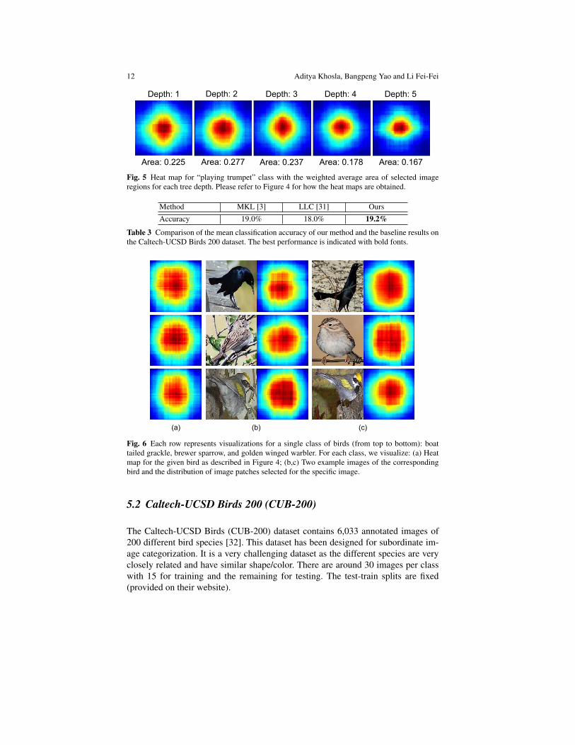
Furthermore, we also demonstrate that the method learns a coarse-to-fine regionof interest for identification. This is similar to the human visual system which isbelieved to analyze raw input in order from low to high spatial frequencies or fromlarge global shapes to smaller local ones [5]. Figure 5 shows the heat map of thearea selected by our classifier as we consider different depths of the decision tree.We observe that our random forest follows a similar coarse-to-fine structure. Theaverage area of the patches selected reduces as the tree depth increases. This showsthat the classifier first starts with more global features or high frequency features to
3 The baseline results are available from the dataset website:http://ai.stanford.edu/˜bangpeng/ppmi
Title Suppressed Due to Excessive Length 11
Instrument BoW Grouplet [33] SPM [21] LLC [31] Ours
Bassoon 73.6 78.5 84.6 85.0 86.2Erhu 82.2 87.6 88.0 89.5 89.8Flute 86.3 95.7 95.3 97.3 98.6French horn 79.0 84.0 93.2 93.6 97.3Guitar 85.1 87.7 93.7 92.4 93.0Saxophone 84.4 87.7 89.5 88.2 92.4Violin 80.6 93.0 93.4 96.3 95.7Trumpet 69.3 76.3 82.5 86.7 90.0Cello 77.3 84.6 85.7 82.3 86.7Clarinet 70.5 82.3 82.7 84.8 90.4Harp 75.0 87.1 92.1 93.9 92.8Recorder 73.0 76.5 78.0 79.1 92.8Average 78.0 85.1 88.2 89.2 92.1
Table 2 Comparison of mean Average Precision (% mAP) of the results obtained by differentmethods on the PPMI binary classification tasks of people playing and holding different musi-cal instruments. Each column shows the results obtained from one method. The best results arehighlighted with bold fonts.
(a) flute (b) guitar (c) violin
Fig. 4 (a) Heat map of the dominant regions of interest selected by our method for playing flute onimages of playing flute (top row) and holding a flute without playing it (bottom row). (b,c) showssimilar images for guitar and violin, respectively. The heat maps are obtained by aggregating imageregions of all the tree nodes in the random forest weighted by the probability of the correspondingclass. Red indicates high frequency and blue indicates low frequency.
discriminate between multiple classes, and finally zeros in on the specific discrimi-native regions for some particular classes.
12 Aditya Khosla, Bangpeng Yao and Li Fei-Fei
Depth: 1 Depth: 2 Depth: 3 Depth: 4 Depth: 5
Area: 0.225 Area: 0.277 Area: 0.237 Area: 0.178 Area: 0.167
Fig. 5 Heat map for “playing trumpet” class with the weighted average area of selected imageregions for each tree depth. Please refer to Figure 4 for how the heat maps are obtained.
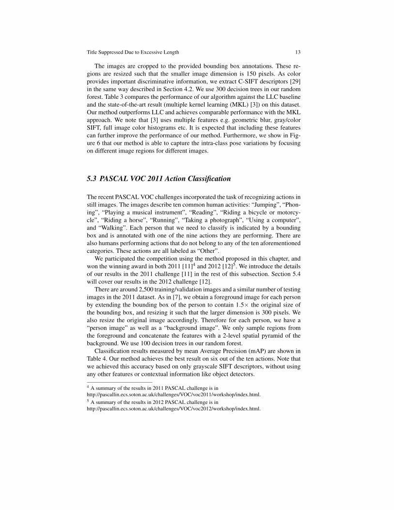
Method MKL [3] LLC [31] Ours
Accuracy 19.0% 18.0% 19.2%
Table 3 Comparison of the mean classification accuracy of our method and the baseline results onthe Caltech-UCSD Birds 200 dataset. The best performance is indicated with bold fonts.
(a) (b) (c)
Fig. 6 Each row represents visualizations for a single class of birds (from top to bottom): boattailed grackle, brewer sparrow, and golden winged warbler. For each class, we visualize: (a) Heatmap for the given bird as described in Figure 4; (b,c) Two example images of the correspondingbird and the distribution of image patches selected for the specific image.
5.2 Caltech-UCSD Birds 200 (CUB-200)
The Caltech-UCSD Birds (CUB-200) dataset contains 6,033 annotated images of200 different bird species [32]. This dataset has been designed for subordinate im-age categorization. It is a very challenging dataset as the different species are veryclosely related and have similar shape/color. There are around 30 images per classwith 15 for training and the remaining for testing. The test-train splits are fixed(provided on their website).
Title Suppressed Due to Excessive Length 13
The images are cropped to the provided bounding box annotations. These re-gions are resized such that the smaller image dimension is 150 pixels. As colorprovides important discriminative information, we extract C-SIFT descriptors [29]in the same way described in Section 4.2. We use 300 decision trees in our randomforest. Table 3 compares the performance of our algorithm against the LLC baselineand the state-of-the-art result (multiple kernel learning (MKL) [3]) on this dataset.Our method outperforms LLC and achieves comparable performance with the MKLapproach. We note that [3] uses multiple features e.g. geometric blur, gray/colorSIFT, full image color histograms etc. It is expected that including these featurescan further improve the performance of our method. Furthermore, we show in Fig-ure 6 that our method is able to capture the intra-class pose variations by focusingon different image regions for different images.
5.3 PASCAL VOC 2011 Action Classification
The recent PASCAL VOC challenges incorporated the task of recognizing actions instill images. The images describe ten common human activities: “Jumping”, “Phon-ing”, “Playing a musical instrument”, “Reading”, “Riding a bicycle or motorcy-cle”, “Riding a horse”, “Running”, “Taking a photograph”, “Using a computer”,and “Walking”. Each person that we need to classify is indicated by a boundingbox and is annotated with one of the nine actions they are performing. There arealso humans performing actions that do not belong to any of the ten aforementionedcategories. These actions are all labeled as “Other”.
We participated the competition using the method proposed in this chapter, andwon the winning award in both 2011 [11]4 and 2012 [12]5. We introduce the detailsof our results in the 2011 challenge [11] in the rest of this subsection. Section 5.4will cover our results in the 2012 challenge [12].
There are around 2,500 training/validation images and a similar number of testingimages in the 2011 dataset. As in [7], we obtain a foreground image for each personby extending the bounding box of the person to contain 1.5× the original size ofthe bounding box, and resizing it such that the larger dimension is 300 pixels. Wealso resize the original image accordingly. Therefore for each person, we have a“person image” as well as a “background image”. We only sample regions fromthe foreground and concatenate the features with a 2-level spatial pyramid of thebackground. We use 100 decision trees in our random forest.
Classification results measured by mean Average Precision (mAP) are shown inTable 4. Our method achieves the best result on six out of the ten actions. Note thatwe achieved this accuracy based on only grayscale SIFT descriptors, without usingany other features or contextual information like object detectors.
4 A summary of the results in 2011 PASCAL challenge is inhttp://pascallin.ecs.soton.ac.uk/challenges/VOC/voc2011/workshop/index.html.5 A summary of the results in 2012 PASCAL challenge is inhttp://pascallin.ecs.soton.ac.uk/challenges/VOC/voc2012/workshop/index.html.
14 Aditya Khosla, Bangpeng Yao and Li Fei-Fei
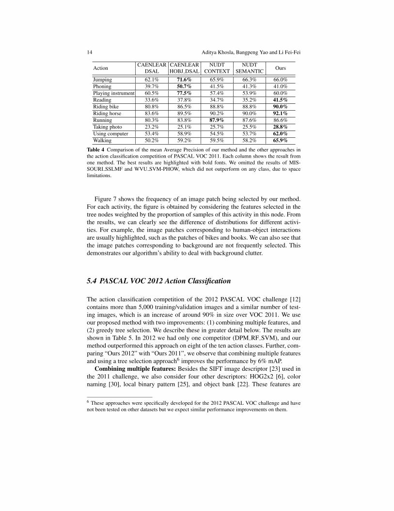
Action CAENLEAR CAENLEAR NUDT NUDT OursDSAL HOBJ DSAL CONTEXT SEMANTIC
Jumping 62.1% 71.6% 65.9% 66.3% 66.0%Phoning 39.7% 50.7% 41.5% 41.3% 41.0%Playing instrument 60.5% 77.5% 57.4% 53.9% 60.0%Reading 33.6% 37.8% 34.7% 35.2% 41.5%Riding bike 80.8% 86.5% 88.8% 88.8% 90.0%Riding horse 83.6% 89.5% 90.2% 90.0% 92.1%Running 80.3% 83.8% 87.9% 87.6% 86.6%Taking photo 23.2% 25.1% 25.7% 25.5% 28.8%Using computer 53.4% 58.9% 54.5% 53.7% 62.0%Walking 50.2% 59.2% 59.5% 58.2% 65.9%
Table 4 Comparison of the mean Average Precision of our method and the other approaches inthe action classification competition of PASCAL VOC 2011. Each column shows the result fromone method. The best results are highlighted with bold fonts. We omitted the results of MIS-SOURI SSLMF and WVU SVM-PHOW, which did not outperform on any class, due to spacelimitations.
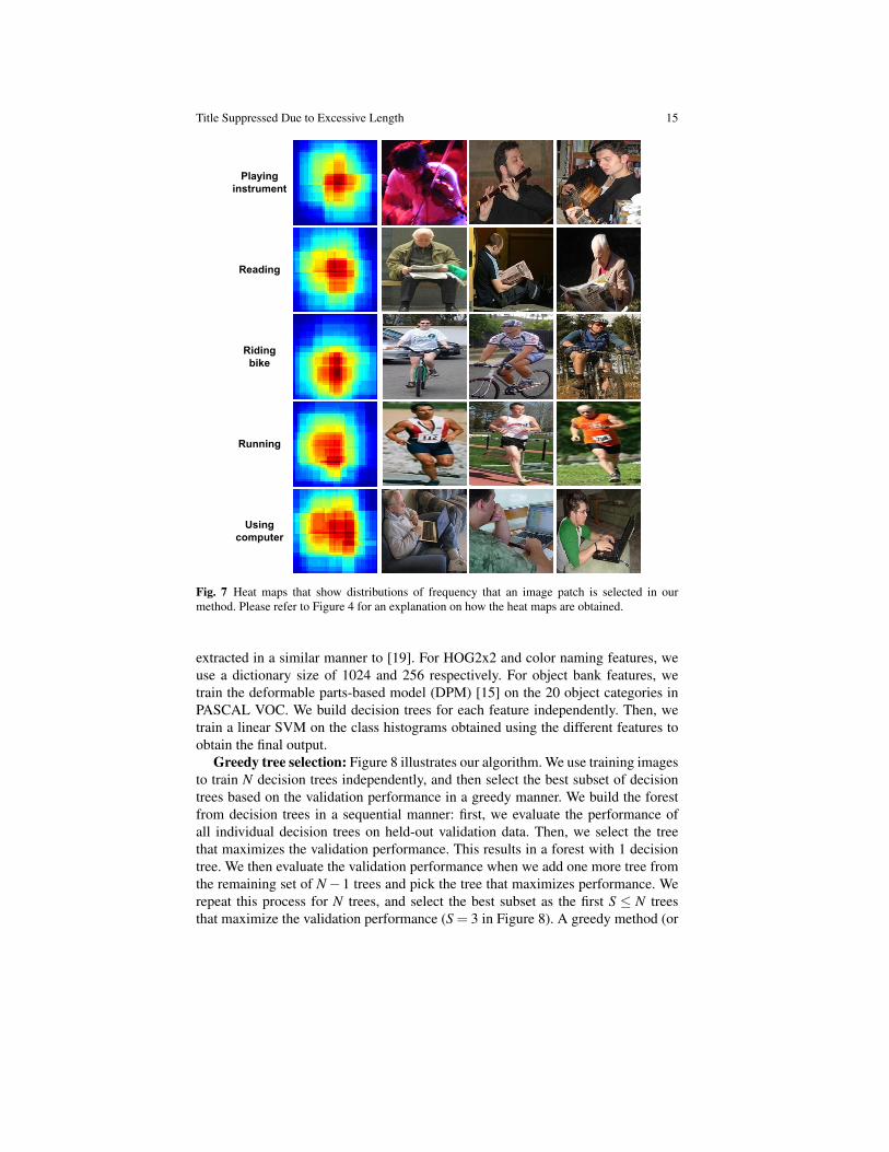
Figure 7 shows the frequency of an image patch being selected by our method.For each activity, the figure is obtained by considering the features selected in thetree nodes weighted by the proportion of samples of this activity in this node. Fromthe results, we can clearly see the difference of distributions for different activi-ties. For example, the image patches corresponding to human-object interactionsare usually highlighted, such as the patches of bikes and books. We can also see thatthe image patches corresponding to background are not frequently selected. Thisdemonstrates our algorithm’s ability to deal with background clutter.
5.4 PASCAL VOC 2012 Action Classification
The action classification competition of the 2012 PASCAL VOC challenge [12]contains more than 5,000 training/validation images and a similar number of test-ing images, which is an increase of around 90% in size over VOC 2011. We useour proposed method with two improvements: (1) combining multiple features, and(2) greedy tree selection. We describe these in greater detail below. The results areshown in Table 5. In 2012 we had only one competitor (DPM RF SVM), and ourmethod outperformed this approach on eight of the ten action classes. Further, com-paring “Ours 2012” with “Ours 2011”, we observe that combining multiple featuresand using a tree selection approach6 improves the performance by 6% mAP.
Combining multiple features: Besides the SIFT image descriptor [23] used inthe 2011 challenge, we also consider four other descriptors: HOG2x2 [6], colornaming [30], local binary pattern [25], and object bank [22]. These features are
6 These approaches were specifically developed for the 2012 PASCAL VOC challenge and havenot been tested on other datasets but we expect similar performance improvements on them.
Title Suppressed Due to Excessive Length 15
Playing
instrument
Reading
Riding
bike
Running
Using
computer
Fig. 7 Heat maps that show distributions of frequency that an image patch is selected in ourmethod. Please refer to Figure 4 for an explanation on how the heat maps are obtained.
extracted in a similar manner to [19]. For HOG2x2 and color naming features, weuse a dictionary size of 1024 and 256 respectively. For object bank features, wetrain the deformable parts-based model (DPM) [15] on the 20 object categories inPASCAL VOC. We build decision trees for each feature independently. Then, wetrain a linear SVM on the class histograms obtained using the different features toobtain the final output.
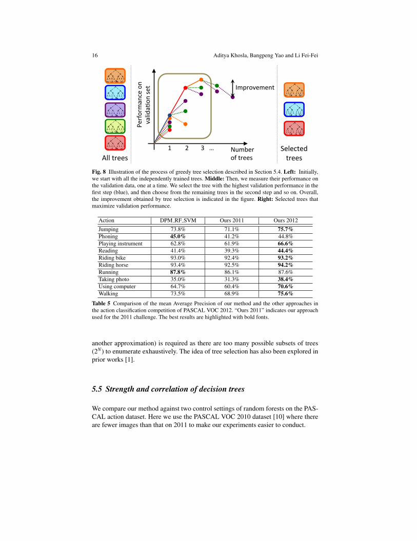
Greedy tree selection: Figure 8 illustrates our algorithm. We use training imagesto train N decision trees independently, and then select the best subset of decisiontrees based on the validation performance in a greedy manner. We build the forestfrom decision trees in a sequential manner: first, we evaluate the performance ofall individual decision trees on held-out validation data. Then, we select the treethat maximizes the validation performance. This results in a forest with 1 decisiontree. We then evaluate the validation performance when we add one more tree fromthe remaining set of N−1 trees and pick the tree that maximizes performance. Werepeat this process for N trees, and select the best subset as the first S ≤ N treesthat maximize the validation performance (S = 3 in Figure 8). A greedy method (or
16 Aditya Khosla, Bangpeng Yao and Li Fei-Fei
Greedy(Tree(Selec+on(
All(trees(
Performance(on(
valida+
on(se
t(Number((of(trees(
1( 2( 3(((…(
Improvement(
Selected((trees(
Fig. 8 Illustration of the process of greedy tree selection described in Section 5.4. Left: Initially,we start with all the independently trained trees. Middle: Then, we measure their performance onthe validation data, one at a time. We select the tree with the highest validation performance in thefirst step (blue), and then choose from the remaining trees in the second step and so on. Overall,the improvement obtained by tree selection is indicated in the figure. Right: Selected trees thatmaximize validation performance.
Action DPM RF SVM Ours 2011 Ours 2012
Jumping 73.8% 71.1% 75.7%Phoning 45.0% 41.2% 44.8%Playing instrument 62.8% 61.9% 66.6%Reading 41.4% 39.3% 44.4%Riding bike 93.0% 92.4% 93.2%Riding horse 93.4% 92.5% 94.2%Running 87.8% 86.1% 87.6%Taking photo 35.0% 31.3% 38.4%Using computer 64.7% 60.4% 70.6%Walking 73.5% 68.9% 75.6%
Table 5 Comparison of the mean Average Precision of our method and the other approaches inthe action classification competition of PASCAL VOC 2012. “Ours 2011” indicates our approachused for the 2011 challenge. The best results are highlighted with bold fonts.
another approximation) is required as there are too many possible subsets of trees(2N) to enumerate exhaustively. The idea of tree selection has also been explored inprior works [1].
5.5 Strength and correlation of decision trees
We compare our method against two control settings of random forests on the PAS-CAL action dataset. Here we use the PASCAL VOC 2010 dataset [10] where thereare fewer images than that on 2011 to make our experiments easier to conduct.
Title Suppressed Due to Excessive Length 17
0 100 200 300 4000.2
0.3
0.4
0.5
0.6
0.7
Number of trees
Mean A
vera
ge-P
recis
ion
dense feature, weak classifier
SPM feature, strong classifier
dense feature, strong classifier
(a) Mean average precision (mAP).
0 100 200 300 400-0.2
-0.1
0
0.1
0.2
Number of trees
Str
ength
dense feature, weak classifier
SPM feature, strong classifier
dense feature, strong classifier
Higher Strength,
Better generalizability
(b) Strength of the decision trees.
0 100 200 300 4000
0.1
0.2
0.3
0.4
0.5
Number of trees
Corr
ela
tion
dense feature, weak classifier
SPM feature, strong classifier
dense feature, strong classifier
Lower correlation,
Better generalizability
(c) Correlation between the decision trees
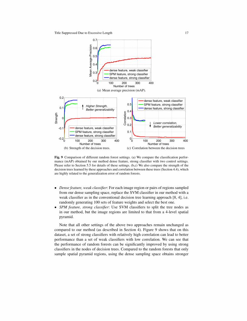
Fig. 9 Comparison of different random forest settings. (a) We compare the classification perfor-mance (mAP) obtained by our method dense feature, strong classifier with two control settings.Please refer to Section 5.5 for details of these settings. (b,c) We also compare the strength of thedecision trees learned by these approaches and correlation between these trees (Section 4.4), whichare highly related to the generalization error of random forests.
• Dense feature, weak classifier: For each image region or pairs of regions sampledfrom our dense sampling space, replace the SVM classifier in our method with aweak classifier as in the conventional decision tree learning approach [8, 4], i.e.randomly generating 100 sets of feature weights and select the best one.
• SPM feature, strong classifier: Use SVM classifiers to split the tree nodes asin our method, but the image regions are limited to that from a 4-level spatialpyramid.
Note that all other settings of the above two approaches remain unchanged ascompared to our method (as described in Section 4). Figure 9 shows that on thisdataset, a set of strong classifiers with relatively high correlation can lead to betterperformance than a set of weak classifiers with low correlation. We can see thatthe performance of random forests can be significantly improved by using strongclassifiers in the nodes of decision trees. Compared to the random forests that onlysample spatial pyramid regions, using the dense sampling space obtains stronger
18 Aditya Khosla, Bangpeng Yao and Li Fei-Fei
trees without significantly increasing the correlation between different trees, therebyimproving the classification performance. Furthermore, the performance of the ran-dom forests using discriminative node classifiers converges with a small number ofdecision trees, indicating that our method is more efficient than the conventionalrandom forest approach. In our experiment, the two settings and our method need asimilar amount of time to train a single decision tree.
Additionally, we show the effectiveness of random binary assignment of classlabels (Section 4.3) when we train classifiers for each tree node. Here we ignore thisstep and train a one-vs-all multi-class SVM for each sampled image region or pairsof regions. In this case C sets of weights are obtained when there are C classes ofimages at the current node. The best set of weights is selected using information gainas before. This setting leads to deeper and significantly unbalanced trees, and theperformance decreases to 58.1% with 100 trees. Furthermore, it is highly inefficientas it does not scale well with increasing number of classes.
6 Summary
In this chapter, we propose a random forest with discriminative decision trees al-gorithm to explore a dense sampling space for fine-grained image categorization.Experimental results on subordinate classification and activity classification showthat our method achieves state-of-the-art performance and discovers much semanti-cally meaningful information. One direction for future work is to extend the methodto allow for more flexible regions where their location can vary from image to im-age. Furthermore, it would be interesting to apply other classifiers with analyticalsolutions such as Linear Discriminant Analysis to speed up the training procedure7.
References
1. Simon Bernard, Laurent Heutte, and Sebastien Adam. On the selection of decision trees inrandom forests. In Neural Networks, 2009. IJCNN 2009. International Joint Conference on,pages 302–307. IEEE, 2009.
2. A. Bosch, A. Zisserman, and X. Munoz. Image classification using random forests and ferns.In Proceedings of the IEEE International Conference on Computer Vision (ICCV), 2007.
3. Steve Branson, Catherine Wah, Boris Babenko, Florian Schroff, Peter Welinder, Pietro Perona,and Serge Belongie. Visual recognition with humans in the loop. In Proceedings of theEuropean Conference on Computer Vision (ECCV), 2010.
4. Leo Breiman. Random forests. Machine Learning, 45:5–32, 2001.
7 Acknowledgements: L.F-F. is partially supported by an NSF CAREER grant (IIS-0845230), anONR MURI grant, the DARPA VIRAT program and the DARPA Mind’s Eye program. B.Y. is par-tially supported by the SAP Stanford Graduate Fellowship, and the Microsoft Research Fellowship.A.K. is partially supported by the Facebook Fellowship.
Title Suppressed Due to Excessive Length 19
5. Charles A. Collin and Patricia A. McMullen. Subordinate-level categorization relies on highspatial frequencies to a greater degree than basic-level categorization. Perception & Psy-chophysics, 67(2):354–364, 2005.
6. N. Dalal and B. Triggs. Histograms of oriented gradients for human detection. In Proceedingsof the IEEE Conference on Computer Vision and Pattern Recognition (CVPR), 2005.
7. Vincent Delaitre, Ivan Laptev, and Josef Sivic. Recognizing human actions in still images: Astudy of bag-of-features and part-based representations. In Proceedings of the British MachineVision Conference (BMVC), 2010.
8. T.G. Dietterich. An experimental comparison of three methods for constructing ensembles ofdecision trees: Bagging, boosting, and randomization. Machine Learning, 40:139–157, 2000.
9. Genquan Duan, Chang Huang, Haizhou Ai, and Shihong Lao. Boosting associated pairingcomparison features for pedestrian detection. In Proceedings of the Workshop on VisualSurveillance, 2009.
10. M. Everingham, L. Van Gool, C. Williams, J. Winn, and A. Zisserman. The PASCAL VisualObject Classes Challenge 2010 (VOC2010) Results, 2010.
11. M. Everingham, L. Van Gool, C. Williams, J. Winn, and A. Zisserman. The PASCAL VisualObject Classes Challenge 2011 (VOC2011) Results, 2011.
12. M. Everingham, L. Van Gool, C. Williams, J. Winn, and A. Zisserman. The PASCAL VisualObject Classes Challenge 2011 (VOC2012) Results, 2012.
13. L. Fei-Fei and P. Perona. A Bayesian hierarchical model for learning natural scene categories.In Proceedings of the IEEE Conference on Computer Vision and Pattern Recognition (CVPR),2005.
14. Li Fei-Fei, Rob Fergus, and Antonio Torralba. Recognizing and learning object categories.Short Course in the IEEE International Conference on Computer Vision, 2009.
15. P. Felzenszwalb, R. Girshick, D. McAllester, and D. Ramanan. Object detection with dis-criminantly trained part-based models. IEEE Transactions on Pattern Analysis and MachineIntelligence, 32:1627–1645, 2010.
16. R. Fergus, P. Perona, and A. Zisserman. Object class recognition by unsupervised scale-invariant learning. In Proceedings of the IEEE International Conference on Computer Vision(ICCV), 2003.
17. Aharon Bar Hillel and Daphna Weinshall. Subordinate class recognition using relational ob-ject models. In Proceedings of the Conference on Neural Information Processing Systems(NIPS), 2007.
18. Kathy E. Johnson and Amy T. Eilers. Effects of knowledge and development on subordinatelevel categorization. Cognitive Development, 13(4):515–545, 1998.
19. Aditya Khosla, Jianxiong Xiao, Antonio Torralba, and Aude Oliva. Memorability of imageregions. In Advances in Neural Information Processing Systems (NIPS), Lake Tahoe, USA,December 2012.
20. Aditya Khosla, Bangpeng Yao, Nityananda Jayadevaprakash, and Li Fei-Fei. Novel dataset forfine-grained image categorization. In First Workshop on Fine-Grained Visual Categorization,IEEE Conference on Computer Vision and Pattern Recognition, Colorado Springs, CO, 2011.
21. S. Lazebnik, C. Schmid, and J. Ponce. Beyond bags of features: Spatial pyramid matching forrecognizing natural scene categories. In Proceedings of the IEEE Conference on ComputerVision and Pattern Recognition (CVPR), 2006.
22. L.-J. Li, H. Su, E. Xing, and L. Fei-Fei. Object bank: A high-level image representation forscene classification and semantic feature sparsification. In Proceedings of the Conference onNeural Information Processing Systems (NIPS), 2010.
23. David G. Lowe. Distinctive image features from scale-invariant keypoints. InternationalJournal of Computer Vision, 60(2):91–110, 2004.
24. Frank Moosmann, Bill Triggs, and Frederic Jurie. Fast discriminative visual codebooks us-ing randomized clustering forests. In Proceedings of the Conference on Neural InformationProcessing Systems (NIPS), 2007.
25. T. Ojala, M. Pietikainen, and D. Harwood. Performance evaluation of texture measures withclassification based on kullback discrimination of distributions. In Proceedings of the IEEEInternational Conference on Pattern Recognition (ICPR), 1994.
20 Aditya Khosla, Bangpeng Yao and Li Fei-Fei
26. A. Oliva and A. Torralba. Modeling the shape of the scene: a holistic representation of theshape envelope. International Journal of Computer Vision, 42(3):145–175, 2001.
27. Jamie Shotton, Matthew Johnson, and Roberto Cipolla. Semantic texton forests for imagecategorization and segmentation. In Proceedings of the IEEE Conference on Computer Visionand Pattern Recognition (CVPR), 2008.
28. Zhuowen Tu. Probabilistic boosting-tree: Learning discriminative models for classification,recognition, and clustering. In Proceedings of the IEEE International Conference on Com-puter Vision (ICCV), 2005.
29. K.E.A. van de Sande, T. Gevers, and C.G.M. Snoek. Evaluating color descriptors for objectand scene recognition. IEEE Transactions on Pattern Analysis and Machine Intelligence,32(9):1582–1596, 2010.
30. J. van de Weijer, C. Schmid, J. Verbeek, and D. Larlus. Learning color names for real-worldapplications. IEEE Transactions on Image Processing, 18(7):1512–1523, 2009.
31. Jinjun Wang, Jianchao Yang, Kai Yu, Fengjun Lv, Thomas Huang, and Yihong Gong.Locality-constrained linear coding for image classification. In Proceedings of the IEEE Con-ference on Computer Vision and Pattern Recognition (CVPR), 2010.
32. Peter Welinder, Steve Branson, Takeshi Mita, Catherine Wah, Florian Schroff, Serge Belongie,and Pietro Perona. Caltech-UCSD birds 200. Technical Report CNS-TR-201, Caltech, 2010.
33. B. Yao and L. Fei-Fei. Grouplet: A structured image representation for recognizing human andobject interactions. In Proceedings of the IEEE Conference on Computer Vision and PatternRecognition (CVPR), 2010.
34. B. Yao and L. Fei-Fei. Modeling mutual context of object and human pose in human-objectinteraction activities. In Proceedings of the IEEE Conference on Computer Vision and PatternRecognition (CVPR), 2010.
35. B. Yao, X. Jiang, A. Khosla, A. L. Lin, L. J. Guibas, and Li Fei-Fei. Human action recognitionby learning bases of action attributes and parts. In Proceedings of the IEEE InternationalConference on Computer Vision (ICCV), 2011.
36. B. Yao, A. Khosla, and L. Fei-Fei. Classifying actions and measuring action similarity bymodeling the mutual context of objects and human poses. In Proceedings of the InternationalConference on Machine Learning (ICML), 2011.
37. B. Yao, A. Khosla, and L. Fei-Fei. Combining randomization and discrimination for fine-grained image categorization. In Proceedings of the IEEE Conference on Computer Visionand Pattern Recognition (CVPR), 2011.
38. Bangpeng Yao, Gary Bradski, and Li Fei-Fei. A codebook-free and annotation-free approachfor fine-grained image categorization. In Proceedings of the IEEE Conference on ComputerVision and Pattern Recognition (CVPR), 2012.
39. Bangpeng Yao and Li Fei-Fei. Action recognition with exemplar based 2.5D graph matching.In Proceedings of the European Conference on Computer Vision (ECCV), 2012.