Integrating ﬁeld sampling, geostatistics and remote ... · J. Arieira et al.: Integrating ﬁeld...

Biogeosciences, 8, 667–686, 2011www.biogeosciences.net/8/667/2011/doi:10.5194/bg-8-667-2011© Author(s) 2011. CC Attribution 3.0 License.

Biogeosciences

Integrating field sampling, geostatistics and remote sensing to mapwetland vegetation in the Pantanal, Brazil

J. Arieira 1,4, D. Karssenberg2, S. M. de Jong2, E. A. Addink 2, E. G. Couto3, C. Nunes da Cunha1,4, and J. O. Skøien2

1Instituto Nacional deAreasUmidas (INAU), Federal University of Mato Grosso, Cuiaba-MT, 78060-900, Brazil2Department of Physical Geography, Faculty of Geosciences, Utrecht University, P.O. Box 80115, 3508 TC, Utrecht,The Netherlands3Department of Soils, Faculty of Agronomy, Federal University of Mato Grosso, Cuiaba-MT, 78060-900, Brazil4Nucleo de estudos ecologicos do Pantanal (NEPA), Instituto de Biociencias, Federal University of Mato Grosso,Cuiaba-MT, 78060-900, Brazil

Received: 23 August 2010 – Published in Biogeosciences Discuss.: 13 September 2010Revised: 11 February 2011 – Accepted: 9 March 2011 – Published: 17 March 2011

Abstract. Development of efficient methodologies for map-ping wetland vegetation is of key importance to wetland con-servation. Here we propose the integration of a number ofstatistical techniques, in particular cluster analysis, universalkriging and error propagation modelling, to integrate obser-vations from remote sensing and field sampling for mappingvegetation communities and estimating uncertainty. The ap-proach results in seven vegetation communities with a knownfloral composition that can be mapped over large areas us-ing remotely sensed data. The relationship between remotelysensed data and vegetation patterns, captured in four factorialaxes, were described using multiple linear regression mod-els. There were then used in a universal kriging procedureto reduce the mapping uncertainty. Cross-validation proce-dures and Monte Carlo simulations were used to quantify theuncertainty in the resulting map. Cross-validation showedthat accuracy in classification varies according with the com-munity type, as a result of sampling density and configura-tion. A map of uncertainty derived from Monte Carlo simu-lations revealed significant spatial variation in classification,but this had little impact on the proportion and arrangementof the communities observed. These results suggested thatmapping improvement could be achieved by increasing thenumber of field observations of those communities with ascattered and small patch size distribution; or by includinga larger number of digital images as explanatory variablesin the model. Comparison of the resulting plant communitymap with a flood duration map, revealed that flooding dura-

Correspondence to:J. Arieira([email protected])

tion is an important driver of vegetation zonation. This map-ping approach is able to integrate field point data and high-resolution remote-sensing images, providing a new basis tomap wetland vegetation and allow its future application inhabitat management, conservation assessment and long-termecological monitoring in wetland landscapes.

1 Introduction

Wetlands are vulnerable habitats threatened by climaticchange, due to their high sensitivity to the hydrologicalregime (Junk, 2002). They form transitional habitats be-tween aquatic and terrestrial systems and embody differentkinds of habitats such as mangroves, peatlands, freshwaterswamps and marshes (Mitsch et al., 2009). The ecologi-cal importance of these habitats has been recognized world-wide as well as the urgent need to preserve them, as stressedin the Cuiaba Declaration on Wetland elaborated during the8th International Wetlands Conference of INTECOL, Brazil.However, lack of policy guidance to regulate the sustainableuse of wetlands may lead to arbitrary management decisions(Junk et al., 2006). To improve the protection of wetlands, itis imperative to have a thorough understanding of the struc-turing elements and of the identification of efficient methodsto describe and monitor them.

Vegetation communities have distinct spatial and tempo-ral patterns. Understanding the mechanisms that determinethese patterns has been an important issue in ecology fordecades (e.g., Connell and Slatyer, 1977; Svenning et al.,2004). Two aspects play a key role: spatial interactions inecological processes (e.g. competition), and environmental

Published by Copernicus Publications on behalf of the European Geosciences Union.

http://creativecommons.org/licenses/by/3.0/

668 J. Arieira et al.: Integrating field sampling, geostatistics and remote sensing to map wetland vegetation

factors (e.g. flooding duration) (Tilman, 1988). Ecologicalprocesses include interactions between individuals, whichmay cause particular spatial patterns in the distribution ofplants. Spatial variation in environmental factors causes spa-tial patterns in vegetation communities due to the differencesof species requirements. These two factors do not usuallyoperate independently but act together at different spatio-temporal scales (Turner, 1989; Svenning et al., 2004). Thismulti-scale interaction may lead to complex spatial patternsthat are continuously changing (Wagner and Fortin, 2005).Consequently, the ability to distinguish plant communitiesthat arise from multi-scale ecological processes requires anunderstanding of the processes and parameters causing theheterogeneity (Turner, 1989).

Classical methods describing vegetation distribution pat-terns along environmental gradients (e.g. altitude, tempera-ture, water, nutrients) are based on sampling field plots, oftenalong transects (McIntosh, 1958; Whittaker, 1967). Such anapproach yields detailed insights into the vegetation occur-rence and vegetation assemblages but does not provide spa-tially continuous information required to study mechanisticprocesses and spatial patterns of the landscape (Austin andSmith, 1989). To retrieve such spatially continuous informa-tion requires techniques that consider space explicitly (Gard-ner and Engelhardt, 2008). One of these techniques is remotesensing. By using the spectral signature of different vegeta-tion states, remote sensing enables description of spatial andtemporal patterns of vegetation in a spatially continuous way(Jensen, 2007). A restriction of this approach is the limitedlevel of detail in attribute information that can be mapped byremote sensing, hindering the detection and identification ofmany ecologically important properties of vegetation com-munities, such as floral composition (Chambers et al., 2007).

Whereas field plots and remotely sensed data each havetheir limitations as a basis for continuous vegetation maps,is it possible to combine them through a statistical approach(Guisan and Zimmerman, 2000; Ferrier et al., 2002; Pfefferet al., 2003; Miller et al., 2007). Point-data or other fielddata and spatially continuous information from remote sens-ing are here incorporated by means of statistical methods,such as ordination analysis (Jongman et al., 1995) and spa-tial interpolation techniques such as kriging. In this way, wecan make maps representing the spatial distribution of vege-tation across large areas that incorporate detailed informationon floral composition (Pfeffer et al., 2003). This approachhas become increasingly important in ecological studies as itrecognizes the influence of spatial correlation in vegetationpatterns (Bascompte and Sole, 1996; Turner et al., 2001). Inaddition, these techniques allow quantification of the uncer-tainty in mapped vegetation, which is valuable when vege-tation maps are used for further quantitative analysis or forcalibration and evaluation of mechanistic vegetation models(e.g., Brzeziecki et al., 1993; Guisan and Zimmerman, 2000;Chong et al., 2001). Here, we will use mapped vegetation(and its uncertainty) to understand the complexity of spatial

patterns of vegetation distribution and to study the effect offlood duration on plant community patterns.

In this study, we integrate field data and remotely senseddata through geostatistical methods for a case study in thePantanal, a 150 000 km2 floodplain of the upper Paraguaybasin in the center-west part of Brazil. The variability inwater depth and flood duration are considered to be the pre-ponderant causes of the high diversity of biological commu-nities and plant zonation patterns found in the area (Junk etal., 1989; Wantzen et al., 2005). In this extensive and pris-tine wetland floodplain, long-term conservation depends onhabitat diversity maintenance (Junk et al., 2006).

The aims of this paper are: (1) to indentify and map plantcommunities of the Pantanal by combining field data andremotely sensed data using advanced statistical techniques;(2) to evaluate the uncertainties in vegetation classificationof this novel statistical approach; and (3) to investigate therelation between flood duration and vegetation zonation.

2 Study area

Our study site covers 60 km2 and is located within a na-ture reserve in North Pantanal (16◦30′–16◦44′ S and 56◦20′–56◦30′ W) (Fig. 1a). The site is representative of a large partof the Pantanal regarding vegetation and environmental con-ditions.

The Pantanal contains a large variety of alluvial ecosys-tems with different drainage patterns, flooding characteris-tics, geomorphologic aspects and vegetation types (Fig. 1a)(Assine and Soares, 2004). The climate of this region istropical humid with marked seasonality between winter andsummer periods (Koppen, 1948). The summer from Novem-ber to April is characterized by high temperatures (averageday temperature 34◦ C) and it is the season with the largestamount of precipitation (Fig. 1b). The precipitation de-creases in winter, causing this season to be very dry (De Mu-sis et al., 1997). The water level in the rivers of the Pantanalfollows the seasonal trend in precipitation. Due to the poorsurface and subsurface drainage and the smooth, low eleva-tion relative to the river level (Alvarenga et al., 1984; Assineand Soares, 2004), large areas of the Pantanal are flooded ev-ery summer. Climate oscillations have been shown to be themain cause of the observed multi-year period of cyclic vari-ation in flooding (Junk et al., 2006). The fluctuation in waterlevel of the river Cuiaba, which crosses the north part of thestudied area, is the main cause of the flooding of the studiedfloodplain.

The Pantanal vegetation presents floristic elements ofthree important morphoclimatic and phytogeographic do-mains i.e. Cerrado (Brazilian savanna), Amazonia and Chaco(Ab’Saber, 1988). Savanna vegetation types are dominantphysiognomies in the Pantanal (67%). Semideciduous for-est, gallery forest, swamp, Chaco, pioneer formations suchas monodominant forest ofVochysia divergensPohl (Silva et

Biogeosciences, 8, 667–686, 2011 www.biogeosciences.net/8/667/2011/

J. Arieira et al.: Integrating field sampling, geostatistics and remote sensing to map wetland vegetation 669

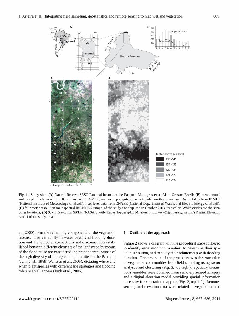
Fig. 1. Study site. (A) Natural Reserve SESC Pantanal located at the Pantanal Mato-grossense, Mato Grosso; Brazil;(B) mean annualwater depth fluctuation of the River Cuiaba (1963–2000) and mean precipitation near Cuiaba, northern Pantanal. Rainfall data from INMET(National Institute of Meteorology of Brazil), river level data from DNAEE (National Department of Waters and Electric Energy of Brazil);(C) four meter resolution multispectral IKONOS-2 image, of the study site acquired in October 2003, true color. White circles are the sam-pling locations;(D) 90-m Resolution SRTM (NASA Shuttle Radar Topographic Mission,http://www2.jpl.nasa.gov/srtm/) Digital ElevationModel of the study area.

al., 2000) form the remaining components of the vegetationmosaic. The variability in water depth and flooding dura-tion and the temporal connections and disconnection estab-lished between different elements of the landscape by meansof the flood pulse are considered the preponderant causes ofthe high diversity of biological communities in the Pantanal(Junk et al., 1989; Wantzen et al., 2005), dictating where andwhen plant species with different life strategies and floodingtolerance will appear (Junk et al., 2006).

3 Outline of the approach

Figure 2 shows a diagram with the procedural steps followedto identify vegetation communities, to determine their spa-tial distribution, and to study their relationship with floodingduration. The first step of the procedure was the extractionof vegetation communities from field sampling using factoranalyses and clustering (Fig. 2, top-right). Spatially contin-uous variables were obtained from remotely sensed imageryand a digital elevation model providing spatial informationnecessary for vegetation mapping (Fig. 2, top-left). Remote-sensing and elevation data were related to vegetation field

www.biogeosciences.net/8/667/2011/ Biogeosciences, 8, 667–686, 2011

http://www2.jpl.nasa.gov/srtm/


Fig. 2. Flow diagram describing the procedural steps in the analysis of the data.

data using regression analysis (Fig. 2, centre). After fittingvariograms describing the spatial correlation in the residualsof the regression analysis, universal kriging was performedto combine extracted factor scores and spatially continuousinformation derived from remote sensing to map vegetationcommunities (Fig. 2, centre). The second step of the proce-dure included an extensive uncertainty analysis on this map-ping procedure by cross-validation and random simulationsto quantify the quality of the vegetation community maps(Fig. 2, bottom-left). Finally, the vegetation map was usedto study the vegetation-environment relations by comparing

spatial patterns of plant community distribution with spatialpatterns of observed flooding duration (Fig. 2, bottom right).

4 Data acquisition

4.1 Vegetation data

We have sampled vegetation data based on field sampling ofkey structural and compositional attributes of the five follow-ing plant life forms as defined by Michin (1989): herbaceousspecies (including gramineous plants), vines, shrubs, and two



h

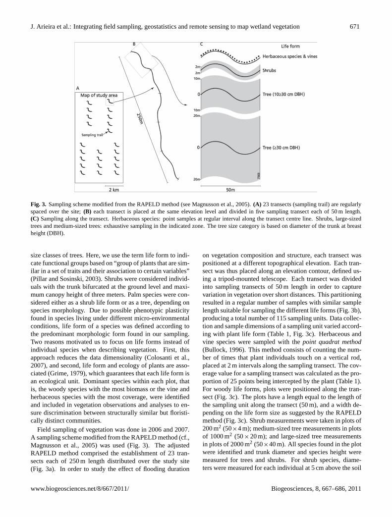
Fig. 3. Sampling scheme modified from the RAPELD method (see Magnusson et al., 2005).(A) 23 transects (sampling trail) are regularlyspaced over the site;(B) each transect is placed at the same elevation level and divided in five sampling transect each of 50 m length.(C) Sampling along the transect. Herbaceous species: point samples at regular interval along the transect centre line. Shrubs, large-sizedtrees and medium-sized trees: exhaustive sampling in the indicated zone. The tree size category is based on diameter of the trunk at breastheight (DBH).

size classes of trees. Here, we use the term life form to indi-cate functional groups based on “group of plants that are sim-ilar in a set of traits and their association to certain variables”(Pillar and Sosinski, 2003). Shrubs were considered individ-uals with the trunk bifurcated at the ground level and maxi-mum canopy height of three meters. Palm species were con-sidered either as a shrub life form or as a tree, depending onspecies morphology. Due to possible phenotypic plasticityfound in species living under different micro-environmentalconditions, life form of a species was defined according tothe predominant morphologic form found in our sampling.Two reasons motivated us to focus on life forms instead ofindividual species when describing vegetation. First, thisapproach reduces the data dimensionality (Colosanti et al.,2007), and second, life form and ecology of plants are asso-ciated (Grime, 1979), which guarantees that each life form isan ecological unit. Dominant species within each plot, thatis, the woody species with the most biomass or the vine andherbaceous species with the most coverage, were identifiedand included in vegetation observations and analyses to en-sure discrimination between structurally similar but floristi-cally distinct communities.

Field sampling of vegetation was done in 2006 and 2007.A sampling scheme modified from the RAPELD method (cf.,Magnusson et al., 2005) was used (Fig. 3). The adjustedRAPELD method comprised the establishment of 23 tran-sects each of 250 m length distributed over the study site(Fig. 3a). In order to study the effect of flooding duration

on vegetation composition and structure, each transect waspositioned at a different topographical elevation. Each tran-sect was thus placed along an elevation contour, defined us-ing a tripod-mounted telescope. Each transect was dividedinto sampling transects of 50 m length in order to capturevariation in vegetation over short distances. This partitioningresulted in a regular number of samples with similar samplelength suitable for sampling the different life forms (Fig. 3b),producing a total number of 115 sampling units. Data collec-tion and sample dimensions of a sampling unit varied accord-ing with plant life form (Table 1, Fig. 3c). Herbaceous andvine species were sampled with thepoint quadrat method(Bullock, 1996). This method consists of counting the num-ber of times that plant individuals touch on a vertical rod,placed at 2 m intervals along the sampling transect. The cov-erage value for a sampling transect was calculated as the pro-portion of 25 points being intercepted by the plant (Table 1).For woody life forms, plots were positioned along the tran-sect (Fig. 3c). The plots have a length equal to the length ofthe sampling unit along the transect (50 m), and a width de-pending on the life form size as suggested by the RAPELDmethod (Fig. 3c). Shrub measurements were taken in plots of200 m2 (50×4 m); medium-sized tree measurements in plotsof 1000 m2 (50×20 m); and large-sized tree measurementsin plots of 2000 m2 (50×40 m). All species found in the plotwere identified and trunk diameter and species height weremeasured for trees and shrubs. For shrub species, diame-ters were measured for each individual at 5 cm above the soil



Table 1. Vegetation data obtained from field sampling and the available remote-sensing and ancillary imagery. Sample size varies with thelife form of plant. Biomass of trees and shrubs are calculated using the allometric equation developed by Chave et al. (2005) and by Barbosaand Ferreira (2004), respectively.ρ is woody density,d is diameter at breast height,H is species height,Cb is circumference at groundheight (cm),n is the number of points touched by a species, andNt is the total number of points in a sample (25 points).

Variable name Calculation Sample size

Vegetation data

Above Ground Woody BiomassTree Eq. (2) 1000 m2

(medium sized tree)2000 m2

(large trees)Shrubs Eq. (1) 200 m2

Canopy height Average height of the overstore (m) 2000 m2

Richness Number of species per areaTree (>30 dbh) 2000 m2

Tree (10< dbh≤ 30) 1000 m2

Shrub 200 m2

herb (including grasses) 25 pointsvine 25 points

% Cover herbs % Cover = (n/Nt) ·100 (%) 25 points% Cover vine % Cover = (n/Nt) ·100 (%) 25 points

Remote-sensing and ancillary data

IKONOS-2 (4 m resolution)blue band (0.45–0.52 µm) Reflectance Values (µm)green band (0.52–0.60 µm)red band (0.63–0.69 µm)infra-red band (0.76–0.90 µm)

NDVI Normalized Difference VegetationIndex NDVI = (NIR− R)/(NIR + R)

Principal ComponentsPC1 Transformation from thePC2 first four multi-spectral bandsPC3 of IKONOS imagesPC4

Digital Elevation Model (90 m resolution) From USGS 7.5′ DEM (meter)

surface and for tree species at breast height. These data werealso used to calculate some variables describing the vege-tation structure. Aboveground biomass of woody individu-als was estimated by two different allometric equations forshrubs and trees, respectively. Aboveground woody biomass(Bs, kg) of shrubs was calculated using the allometric modeldeveloped by Barbosa and Ferreira (2004):

Bs= exp(−3.9041+0.4658 ln(Cb2H)

+0.0458(ln (Cb2H))2)

(1)

with, Cb is circumference at the ground height (cm) andH

the species height (m).

Biomass (Bt, Kg) of a tree species was estimated followingChave et al. (2005):

Bt = 0.112·(ρ ·H ·d2)0.916, (2)

with, ρ (g cm−3) the wood specific density,H (m) thespecies height, andd (cm) the species diameter at breastheight. Information on species densities was obtained fromSchongart et al. (2008). Canopy height (CH) was consideredthe average height of the eight highest individuals in a plot.

4.2 Remote-sensing and ancillary data

Remotely sensed imagery and ancillary data are frequentlyused in spatial vegetation modeling due to their capabilityof providing accurate environmental information related to



vegetation patterns (Guisan and Zimmerman, 2000; Pfef-fer et al., 2003; Miller et al., 2007). An IKONOS-2 imageand a Digital Elevation Model (DEM) (Table 1, Fig. 1c, d)were used in this study to derive variables related to vege-tation patterns. The acquisition date of the IKONOS-2 im-age is 1 October 2003 corresponding to the dry season inthe Pantanal and representing an optimal time for detectingspectral signatures of terrestrial vegetation on the floodplain,due to the availability of cloud free images and nonfloodedsoil conditions. The IKONOS-2 image consists of four spec-tral bands: three bands in the visible part of the spectrumlocated at blue (450–520 nm), green (520–600 nm) and red(630–690 nm) and one band in Near Infrared (760–900 nm)(Table 1). The pixel size is approximately 4×4 m. The reg-istered radiance values by the IKONOS-2 sensor were con-verted to reflectance values using the calibration informationprovided by Bowen (2002). A Normalized Difference Vege-tation Index (NDVI) was computed from the spectral bandsby taking a ratio of the difference of the near infrared and redspectral bands and the sum of the near infrared and red band(Tucker, 1979). Such an NDVI image shows stronger con-trast between vegetation and soil and water surfaces while re-ducing noise in the image. Furthermore, we applied a princi-pal component (PC) transformation to the IKONOS-2 imageto reduce inter-band correlation and extract new spectral in-formation that arises from this transformation. The four orig-inal bands, the NDVI image and the four principal compo-nent images were used for further data analysis as describedin the next section. The 90-m resolution DEM of the studyarea was obtained from the SRTM (NASA Shuttle Radar To-pography Mapping Mission) and used to provide continuousinformation of canopy height rather than soil surface (Jacob-sen, 2006) (Fig. 1d).

The original geodata with cell sizes of 4 m (IKONOS-2) and 90 m (SRTM DEM) were re-sampled to support thefield data, i.e., to the plot size used to take measurementsof large tree species (50×40 m). The disaggregation of the90 m cells into 40×50 m cells was done by overlaying thedesired 40×50 m cells over the 90 m cells and creating in-tersects. From these a weighted average was calculated todetermine the value for the 40×50 m cells. A similar pro-cedure was used to aggregate the 4 m cells of IKONOS-2images into 40×50 m cells. The procedure for extraction ofthe averaged values from the images consists of: (1) delin-eating the irregular plot boundaries in the IKONOS-2 imageusing ARC/INFO GIS software (version 9.0; ESRI, 2006);(2) calculating average remote-sensing and elevation valuesfor exactly these digitized plots; and (3) extracting variablesfrom the IKONOS-2 derived images and SRTM DEM forthe 115 plots to be used in the analysis. The two last stepswere done in the PCRaster interactive raster GIS environ-ment, which is oriented towards spatio-temporal modelling(PCRaster, 2002; Wesseling et al., 1996).

5 Identifying plant communities

Velloso et al. (1991) developed a classification system ofBrazilian vegetation, which was adapted by Nunes da Cunhaet al. (2006), providing a detailed description of the plantcommunities in the Pantanal. Here, we have used the com-munities described by Nunes da Cunha et al. (2006), becausethese can be identified by means of structure and composi-tion (only dominant species) data of different vegetation lay-ers. Communities are represented at a broad level as veg-etation formation types rather than plant associations. Weused factor analysis (Bray and Curtis, 1957) where the factorscores summarize the structural and compositional charac-teristics of different vegetation samples. These factors werefound in a principal component analysis of the correlationmatrix, generating a small number of orthogonal factors ex-plaining the correlation among the vegetation variables (Leg-endre and Legendre, 1998). The different factor scores areplotted against each other in Fig. 4, and the proximity amongpoint-samples and our field background about the vegetationclasses found in these points were used to classify them invegetation classes/clusters.

5.1 Ecological interpretation of ordination space

The first four factor axes explain 46% of the total vari-ance (Table 2). We assumed that the strongest correlationswith each axis reflect the main vegetation gradients cap-tured by it. Factor 1 explains a relatively large proportion(22%) of the total variance. It mainly distinguishes commu-nities dominated by a tall and rich tree layer (negative load-ings) and those dominated by vine, shrub or herbaceous lifeforms (positive loadings). Although explaining considerablysmaller proportions of the total variance, the remaining fac-tors are still useful for identifying the vegetation classes. Fac-tor 2 separates plant communities by their degree of coverageand richness of herbaceous species. Factor 3 mainly repre-sents variation in biomass of two trees,Brosimum latescensandMouriri guianensis, and one shrub,Psychotria capitata.Factor 4 mainly represents variation in the biomass of shrubsand of two species, the medium-sized treeSapium obovatumand the shrubRuprechtia brachycepala.

5.2 Defining plant communities through ecologicalinterpretation of clusters

Plant communities of the study area are identified based onthe proximity of point scores on the ordination space, andthe general expert knowledge (including existing vegetationcommunity classifications) of vegetation communities in thearea. Seven clusters are indicated in a scatter plot of thedifferent factors (Fig. 4) and are classified as:Monodomi-nant forest, Shrubland, Alluvial seasonal semideciduous for-est (Alluvial forest), Alluvial seasonal semideciduous lowforest(Alluvial low forest), Seasonally flooded grass-woody



Fig. 4. Factor analysis biplots of the axes 1 to 4 on vegetation variables obtained from 115 sampling locations. Seven clusters (symbols)represent the vegetation communities found in the studied floodplain. Factor 1 describes the gradient of tree biomass found in the study site;Factor 2 of herb cover and richness; Factor 3 of tree dominant species; and Factor 4 of shrub biomass.

savanna(Grassland), Low open tree and shrub savanna(Open savanna) and Low dense tree and shrub savanna(Dense savanna). The number of samples in each clusterand their distribution over the ordination space express thestructural and floristic variability found within the commu-nity and which communities have dominated the floodplainlandscape. Table 3 provides a statistical summary of struc-tural and floristic characteristics of communities.

A number of communities show overlapping ranges ofscores on some of the factor axes, while other factor axes

provide clear boundaries between these communities. For in-stance, the transitions betweenAlluvial forestandMonodom-inant forestare smooth (Fig. 4a–c). These two communitiesare mainly separated through the tree biomass and coverageof herbaceous species inMonodominant forest(Fig. 4a) andthe dominance ofBrosimum latescensandMouriri guianen-sis in Alluvial fores (Fig. 4b). Dense savannalies betweenOpen savannaandMonodominant forest. Tree biomass dis-tinguishes these communities (Fig. 4a).Dense savanna,Grassland, Open savannaand Monodominant foresthave



Table 2. Summary statistics for the factor analysis. Numbers inbold highlight the highest correlation with the factor axis.

Variable Factor 1 Factor 2 Factor 3 Factor 4

Richness tree −0.76 −0.25 0.17 −0.28Richness shrub 0.28 0.07 0.20 −0.35Richness herb 0.31 0.58 0.43 −0.11Canopy height −0.86 −0.05 −0.33 0.09Cover % herb 0.04 0.79 0.16 0.06Cover % vine 0.82 −0.15 −0.16 0.16Richness vine 0.73 −0.09 −0.14 0.16Biomass tree (total) −0.88 0.00 −0.26 0.18Biomass shrub 0.54 −0.42 0.07 −0.58

Biomass (DBH 10 cm> 30 cm)

Vochysia divergens −0.31 −0.05 0.05 0.03Sapium obovatum −0.03 −0.23 −0.09 −0.56Licania parvifolia −0.43 −0.03 −0.17 0.11Brosimum latescens −0.29 −0.34 0.51 0.22Trichilia catigua −0.30 −0.27 0.45 0.06Duroia duckei −0.59 0.09 −0.35 0.19Cecropia pachystachya −0.31 0.23 −0.20 −0.02Mouriri guianensis −0.51 −0.35 0.36 0.22

Biomass (DHB> 30 cm)

Vochysia divergens −0.72 0.17 −0.47 0.21Mouriri guianensis −0.37 −0.42 0.55 0.23

Biomass (shrub)

Albizia polycephala 0.62 −0.11 0.02 0.12Ruprechtia brachycepala −0.02 −0.25 0.05 −0.50Peritassa dulcis 0.18 −0.52 −0.46 −0.06Melochia villosa 0.41 0.16 0.18 0.24Byrsonima cydoniifolia −0.23 −0.40 0.43 0.15Psychotria capitata −0.48 −0.49 0.51 0.20Bauhinia rufa 0.17 0.04 0.09 −0.32Mimosa pellita 0.57 0.05 0.02 0.35Laetia americana 0.74 −0.20 −0.09 0.14Solanum pseudoauriculatum 0.26 0.19 0.15 0.22Eugenia florida 0.03 −0.29 −0.32 0.07Alchornia discolor −0.22 0.37 0.03 −0.37Mabea paniculata −0.30 0.12 0.17 −0.25Byrsonima orbygniana 0.00 0.19 0.25 −0.49

Cover % herbaceous species

Paspalum hydrophilum 0.34 0.37 0.24 0.05Panicum guianense −0.17 0.06 −0.18 −0.35Scleria bracteata −0.57 0.24 −0.27 0.16

Cover % vine

Cissus spinosa 0.67 −0.31 −0.20 −0.001Aniseia cernua 0.54 0.14 0.09 0.34Paullinia pinata 0.52 −0.31 −0.27 0.09Dolliocarpus dentatus 0.23 −0.57 −0.27 −0.01Ipomea rubens 0.36 0.16 0.17 0.22% Variance 22 9 8 7

similar correlation values with Factor 2, indicating that theremay be a small variation in coverage of herbaceous speciesbetween these communities. The low tree biomass inShrub-land is responsible for its positive scores on the first factor.Alluvial low forestis distinguished from other forests basedon Factor 4. Its high shrub coverage compared toShrub-

landand the dominance ofSapium obovatumandRuprechtiabrachycepalagenerates the lowest scores on Factor 4.

6 Mapping plant communities

6.1 Correlating field data and image derived data

We first examined the relationship between IKONOS imagesand SRTM DEM and the vegetation patterns captured in thefour factorial axes. Pearson correlation was applied to ana-lyze the existence of linear relationships, observed in an ex-ploratory analysis of the data, between image derived vari-ables and field data (scores on factor axes). This facilitatesour understanding of the spectral nature of the field data andthe ecological interpretation of the variables (James and Mc-Culloch, 1990). Next, the relationship between the imagederived variables and the factor axes was found using the fol-lowing multiple linear regression model:

Yi = a0+a1x1i +a2x2i + ...+apxpi +εi (3)

whereYi is the score value,a0,a1,...,ap are the model pa-rameters,x1i, x2i , . . . , xpi are the values of the image de-rived variables andεi are uncorrelated residuals. The anal-yses were done with log transformed reflectance values toensure that the statistical distribution of the data is close toGaussian (Draper and Smith, 1998).

In the multiple regression analysis, image derived vari-ables were selected to be included in the multiple regressionmodels using the best-subset regression method (Hofmannet al., 2007; James and McCulloch, 1990). In this analy-sis all combinations of explanatory variables in regressionsare tested, and Mallow’s C-p statistic (Mallows, 1973) anddetermination coefficients (R2) are used as eliminatory crite-rions of variables (Draper and Smith, 1998). We consider thebest regression equation for each factor the one with the low-est C-p value, highestR2, and lowest number of explanatoryvariables.

6.2 Vegetation patterns captured by digital images

Table 4 shows correlations between explanatory variablesand the factor axes. Except for NDVI, all image derived datapresent significant correlation with Factor 1. The strongestcorrelations with this first axis are found with blue, green andred bands, PC1 and canopy topography. Lower reflectancevalues in the three spectral bands and lower score values inthe PC1-3 images are linked to areas occupied by commu-nities with high stored tree biomass such asMonodominantforest andAlluvial forest (Table 4). Lower score values inthe PC4 reflects communities with lower tree biomass val-ues even though this axis explains the noise from the spec-tral band transformation. In spite of its weak correlationwith Factor 1, NDVI shows an expected spectral behaviour:the values decrease toward areas with lower tree biomass,



Table 3. Structural and floristic characteristics of plant communities, given as mean and standard deviation.

Cha

ract

eris

ticsp

ecie

s

Monodominantforest

Shrubland Alluvialforest

AlluvialLow Forest

Grassland Opensavanna

Densesavanna

VochysiadivergensPohl.

LaetiaamericanaL.

ByrsonimacydoniifoliaA. Juss.

RuprechtiabrachysepalaMeisn.

PaspalumhydrophilumHenrard

PaspalumhydrophilumHenrard

ByrsonimaorbignyanaA. Juss.

Duroia duckeiHuber

Mimosa pellitaHumb. & Bonpl.ex Willd.

PsychotriacapitataRuiz & Pav.

CrataevatapiaL.

PanicumguianenseHitchc.

HybiscusfurcellatusDesr.

Bauhinia rufa(Bong.)Steud.

LicaniaparvifoliaHuber

Peritassa dulcis(Benth.) Miers

TrichiliacatiguaA. Juss.

Banara argutaBriq.

LaetiaamericanaL.

AlchorneadiscolorPoepp.

ScleriabracteataCav.

Albizia polycephala(Benth.) Killip

MouririguianensisAubl.

SapiumobovatumKlotzschex Mull.Arg.

Cissus spinosaCambess.

Brosimumlactescens(S. Moore)C. C. Berg

CecropiapachystachyaTrecul

Aniseia cernuaMoric.

Paullinia pinnataL.

Ipomea rubensChousy

Richness of herbs(no. of sp. persample)

1.98±1.92 2.54±1.75 2±0.82 2.4±1.52 3.67±1.56 4.6±1.34 4.2±1.92

Richness of vines(no. of sp. persample)

2.96±1.52 7.71±1.72 1.71±1.25 4.6±1.82 4.42±1.31 3.8±1.1 1.4±1.52

Richness of shrubs(no. of sp. persample)

7.85±3.58 9.89±2.36 6.71±4.61 6.4±1.95 8.58±2.91 8.6±2.3 14.6±3.6

Richness ofmedium sized trees(no. of sp. persample)

4.91±1.64 0.32±0.61 8±2.65 6.2±2.17 0.17±0.39 1±0.45 5.8±1.64

Richness of largetrees (no. of sp.per sample)

2.77±0.71 0.14±0.45 4.71±1.11 1.6±1.34 0.17±0.39 0.6±0.55 2±0.7

Biomass of shrubs(Mg ha−1)

3.25±6.71 10.11±3.79 3.82±3.01 13.54±8.18 4.03±2.08 2.63±0.78 9.96±6.71

Biomass ofmedium sized trees(Mg ha−1)

109.58±17.29 2.38±7.58 91.54±29.87 28.50±21.78 4.57±9.56 29.5±31.01 26.75±17.29

Biomass of largetrees (Mg ha−1)

84.94±11.36 1.87±6.80 57.15±18.55 9.47±8.41 1.81±4.29 24.8±28.06 9.40±11.36

Canopy height (m) 20.19±1.30 2.41±0.84 15.2±3.19 5.72±1.74 1.76±0.21 2±0.1 3.14±1.3

Cover % herbs 37.06±9.55 27±24.26 16±7.66 18.4±11.52 61.33±21.46 97.6±3.58 56.8±9.55

Cover % vines 21.74±6.07 83±11.71 8.57±6.70 47.2±21.05 43.33±19.66 27.2±7.16 5.6±6.07



Table 4. Pearson’s correlation coefficients between factor axesand image variables: four spectral bands, Normalized DifferenceVegetation Index (NDVI), Principal Component transformation tothe IKONOS-2 image (PC), and canopy topography derived fromDEM-SRTM (DEM).

Variable Factor 1 Factor 2 Factor 3 Factor 4

blue band 0.71∗ 0.30∗ 0.38∗ 0.008green band 0.71∗ 0.23∗ 0.38∗ −0.03red band 0.67∗ 0.36∗ 0.37∗ −0.009infra-red band 0.43∗ −0.34∗ 0.02 −0.001NDVI −0.124 −0.47∗ −0.30∗ 0.01PC1 0.69∗ −0.13 0.25∗ −0.03PC2 0.29∗ 0.61∗ 0.30∗ 0.04PC3 0.26∗ −0.08 0.03 0.10PC4 −0.33∗ 0.13 −0.10 −0.10Canopy −0.72∗ 0.15 −0.39∗ −0.16topography(DEM)

∗ P-value≤ 0.05 for statistical significance.

such as those areas covered byGrassland, Open savanna,ShrublandandDense savanna. The strong negative corre-lation between canopy topography and Factor 1 shows thatthe boundaries between communities dominated by trees andthose dominated by shrubs, lianas and herbs are detected bydifferences in canopy height.

The variability in cover degree and richness of herbaceouslife forms expressed by the second axis is best described bythe PC2 image (61%; Table 4). Communities with higherand richer coverage of herbaceous species such asGrass-land, Open savannaandDense savannaare associated withhigher reflectance values in blue, green and red bands andhigher score values in the PC2 image. The negative correla-tions between Factor 2 and infra-red band and NDVI showthat communities dominated by herbaceous species presentweaker spectral response to these two images.

As observed earlier, Factor 3 mostly justifies the spatialdistribution pattern of three tree species that dominate inAl-luvial forest. Relatively toMonodominant forest, the lowerbiomass content and canopy height ofAlluvial forestmightbe the cause for the negative correlations between Factor 3and NDVI and Factor 3 and canopy topography.

The spatial variability of Factor 4 represents vegetationpatterns that are mainly explained by canopy topography(i.e. DEM) showing that areas with higher biomass of shrubsare associated with lower canopy height.

The equations found in the multiple regression analysisare shown in Table 5. The regression models significantlyexplain 70.4%, 66.3%, 31.3% and 25.6% of the variance infactors 1 to 4, respectively. The use of an automatic variableselection technique to choose regression models resulted ininclusion of autocorrelated predictor variables in the mod-

els, such as the principal component images and IKONOSbands. Because the main purpose of using multiple regres-sion analysis in this study is to predict values accurately, andnot to test hypotheses about the model parameters, colinear-ity of explanatory variables was not a matter of great concern(Legendre and Legendre, 1998).

6.3 Variogram analysis

We applied variogram analysis to the residuals of the mul-tiple linear regression to derive information on their spatialstructure (Wagner and Fortin, 2005). This information wasused for two reasons: (1) to investigate the spatial autocorre-lation associated with the observed vegetation patterns; (2) touse this information when making spatial predictions (Milleret al., 2007). Sample variograms were estimated and vari-ogram models fit using the functionautofitVariogramfromthe library automap(Hiemstra et al., 2008) in the statisti-cal environment R-2.7.2 (R Development Core Team, 2009).The functionautofitVariogramautomatically selects the var-iogram model and parameters that best match the observedsample variogram. The function iterates over the variogrammodels (spherical, Gaussian, Matern, and exponential) andselects the model and model parameters that result in thesmallest residual sum of squares with the sample variogram.

The results indicate that the vegetation gradients repre-sented by the residuals of each factor (Factor 1–4) vary ondifferent spatial scales (Fig. 5). Variograms of the Maternfamily, a family of semivariogram models where the degreeof smoothness of the random field is controlled through ashape parameter (kappa) (Pardo-Iguzquiza and Chica-Olmo,2008), were fit for Factors 1, 2 and 4 (Fig. 5a, b, d), whereasan exponential variogram (special case of the Matern fam-ily) was fit for Factor 3 (Fig. 5c). The first and third fac-tors show large-scale patterns as revealed by their ranges ofspatial dependence. The variogram of Factor 1 has a rangeof 3380 m, whereas the variogram of Factor 3 is monoton-ically increasing within the extent of the sample variogramand consequently has a larger range. The variograms of Fac-tors 2 and 4 show short ranges of spatial dependence (closeto a pure nugget effect) suggesting that processes governingtheir spatial patterns show small scale variability.

6.4 Universal kriging

Universal kriging is a spatial interpolation technique that canincorporate environmental data and spatial dependence in themodeled error to predict at locations without observationsand generate accurate vegetation distribution maps (Pfefferet al., 2003; Pebesma and Wesseling, 1998). Universal krig-ing was done on the regression residuals and the interpo-lated residuals were added to a trend surface to predict factorscores at unobserved locations. This trend surface was basedon the regression equation in Eq. (3) (Pfeffer et al., 2003).The predicted scores were used to create four factor score



Table 5. Multiple linear regression models relating factor axes scores (F1–4) to imagery derived variables: four spectral bands (blue, green,red and infra-red), Normalized Difference Vegetation Index (NDVI), Principal Component transformation to the IKONOS-2 image (PC), andcanopy topography derived from DEM-SRTM (DEM).R2 is the coefficient of determination showing the strength of these relationships.

Equation R2

F1= 30.6 + 9.49 blue− 0.0241 DEM− 34.7 PC1− 46.4 PC2− 33.7 PC3 + 8.7 PC4 + 2.15 NDVI 70.4F2= − 9.43 + 5.15 NDVI + 0.0715 DEM− 3.38 green + 3.52 red + 55.1 PC2− 140 PC3 66.3F3= 15.2 + 419 PC4− 9.98 NDVI + 15.9 blue− 15.2 red + 4.90 infra-red 31.3F4= 2.4− 27.9 PC1 + 53.9 PC2 + 129 PC3− 49 PC4− 0.9 NDVI− 0.15 DEM− 20.9 blue + 2.2 green + 9.8 red + 3.6 infra-red 25.6

Fig. 5. Maps of the kriged estimates of factor scores and the semi-variograms of the residuals of the regression between factor axes andremotely sensed and ancillary data; fitted variogram models: mat: matheron family, exp: exponential. Values between brackets are nuggeteffect, structured variance and variogram range, respectively.(A) Factor 1;(B) Factor 2;(C) Factor 3;(D) Factor 4.



Fig. 6. Maps of the standard deviation of the predicted error result-ing from universal kriging;(A) Factor 1;(B) Factor 2;(C) Factor 3;(D) Factor 4.

maps. In addition, the universal kriging approach was usedto estimate the prediction error (standard deviation), which istypically increasing as a function of the distance to observa-tion locations (Stein and Corsten, 1991).

The score maps in Fig. 5 show the vegetation spatial pat-terns predicted by universal kriging. The score maps of thefirst and third factor axes (Fig. 5a and c) show mainly large-scale variability. These axes, as mentioned earlier, mostlyrepresent spatial variation of tree life forms. Contrarily, thescore maps of the second and fourth axes (Fig. 5b and d)representing the occurrence of herbaceous and shrub layers,respectively, show small-scale spatial variability.

Examining the pattern of the prediction errors of the scoresfor each factor axis (Fig. 6), one can infer to which extentsample data and image data contribute to predictions. Whenthe range of the semivariogram is large, as seen in the semi-variograms of Factor 1 and 3 (Fig. 5a, c), the prediction er-rors increase slowly with the distance away from samples.On the other hand, a short range in the variogram results inprediction errors increasing rapidly with distance away fromsamples, as is the case with Factor 2 and 4. Image data willin this case have greater impact on predictions. Neverthe-less, the quality of the factor score maps is not only related todifferences between small-scale and large-scale spatial vari-ation but rather reflects the explanatory strength of the rela-tionship between factor axes and image derived variables asshown by the mean error in the score maps. We use thesemean errors as indicative of the overall quality of the maps.According to these averages, Factor 1 represents the mostaccurate map (mean standard deviation of 0.51) followed byFactor 2 (mean s.d.= 0.64), Factor 3 (mean s.d.= 0.69) andFactor 4 (mean s.d.= 0.87).

Fig. 7. (A) Predicted distribution of the plant communities iden-tified at the study site.(B) Results of leave-one-sample out cross-validation. Percentage of predicted classes at sampling locations.Each bar shows the results for sampling locations with a certain ob-served class (indicated by the colors at the bottom of theC panel).(C) Idem, leave-five-out cross-validation.N = 115.

6.5 Spatial distribution of plant communities acrossthe floodplain

In the final part of this procedure, we combined score pointdata and the four kriged maps generated as described in theformer sections to create the final map of plant communi-ties. First, the cluster center of each community was calcu-lated as the average of score values of each factor axis. Then,the resulting seven cluster centers were used to assign eachlocation on the map to a community class. This was doneby calculating Euclidean distances between centers and pre-dicted scores values. Each location was then assigned to thecommunity whose center was nearest to the predicted scorevalues at that location.

The map of plant communities (Fig. 7a) resulting from thisclassification method shows the predicted spatial distributionof the seven identified plant communities on the floodplain.Grassland(16% of coverage),Shrubland(30% of cover-age) andMonodominant forest(32% of coverage) sum upto 78% of the coverage at the studied site. These commu-nities mostly appear as large and contiguous patches acrossthe site.Alluvial forestandAlluvial low forest, as expected,appear as strips covering exclusively places close to water



bodies: along rivers, channels and surroundingbaıas, i.e.temporary or permanent lakes seasonally connected to theriver. These two communities cover just 4% (2% each) ofthe studied floodplain. The greatest portion of the 10% ofOpen savannathat covers the study area is located towardsthe Northern boundary. The 8% ofDense savannais foundas small patches generally surrounded byOpen savannaandas a big patch besideMonodominant forest.

6.6 Evaluating uncertainty

Vegetation mapping using statistical approaches carries dif-ferent sources of uncertainties related to sampling scheme,interpolation errors, sampling support, data quality, lack ofdata and others, which may compromise the model’s capa-bility of accurately predicting vegetation patterns (Guisanand Zimmerman, 2000; Pfeffer et al., 2003; Miller et al.,2007). The predictive success of our mapping approach wasevaluated using cross-validation (Efron and Tibshirani, 1986)and random-simulations (Bourennane et al., 2007), both per-formed in R.

6.6.1 Cross-validation

We have used cross-validation to investigate the sensitiv-ity of vegetation predictions performed by universal krig-ing as a result of sampling variability (Pfeffer et al.,2003). Two resampling techniques were applied:leave-one-out cross-validation (LOOCV)andleave-five-out cross-validation (LFOCV). The first technique is the standard pro-cedure (Efron and Tibshirani, 1986) which consists of omit-ting one sample at a time from the data set and based onthe remaining observed values make predictions at this loca-tion using the interpolation technique, i.e., universal kriging.Because samples/plots within the same transect are consider-ably closer to other observations than the typical distance be-tween prediction locations and observations locations (Milleret al., 2007), LFOCV was used to test the prediction qualityof the model when the whole transect, that is, five plots, is leftout to make predictions. Vegetation classes were assignedfrom the predicted scores and compared with the observedvegetation classes at the 115 sample plots.

Overall agreement between predicted and observed classesdoes not differ substantially between the two resamplingtechniques:leave-one-outresults in 52.2% agreement andleave-five-outin 48.7% agreement. Both techniques showthat accuracy in classification varies according to the com-munity type (Fig. 7b and c). Communities which have beenobserved on a large number of plots and occupy large por-tions of the vegetation map, such asMonodominant forestand Shrubland, are less sensitive to sampling density thanthose communities which occur in smaller and few patches,such asAlluvial forestandAlluvial low forest. Consequently,communities observed in few of the plots are wrongly clas-sified also for LOOCV (Fig. 7b). Other possible causes of

uncertainty in classification from our mapping approach de-rives from the similarity between community types havinga small distance between cluster centers in the ordinationspace (Fig. 4). Communities such asAlluvial forest andDense savannaare frequently predicted to be their neigh-boring communities, namely,Monodominant forest; andAl-luvial low forest are frequently predicted to beShrubland(Fig. 7b and c).

6.6.2 Simulation

A Monte Carlo approach was applied to examine the uncer-tainty of our method (Legendre and Legendre, 1998). Inthis approach, we used the same universal kriging equa-tions, however creating equally likely random realizations(i.e., possible random outcomes or scenarios) of score mapsinstead of predicted values as was done in the original proce-dure. This was done by simulating 1000 realizations of scoremaps for each factor, based on the scores at the observationlocations and the fit variograms. These realizations reflectthe prediction uncertainty at the prediction locations; all re-alizations are equally probable. For each realization, we cal-culated the vegetation pattern, using the same Euclidean dis-tance algorithm applied in the original mapping procedure.This was repeated for all 1000 realizations, resulting in 1000realizations of vegetation community maps. Two realizationsare shown in Fig. 8b, c. From these 1000 realizations, we cre-ated a map showing the probability, from 0 to 1, that a certaincommunity is found in a 40 m grid cell (Fig. 8). On this map,a value 1 indicates zero prediction uncertainty.

The result shows that the quality of classification variesspatially, even though the proportion and arrangement ofcommunities observed in the original map is preserved toa great extent. The central zone of a community patch ismore likely to be classified correctly than border areas, asshown by the increasing probabilities towards the center ofpatches of communities (Fig. 8a). This might reflect intrinsicuncertainties in classification of natural ecotones reflected inthe overlapping of score values of very close communitiesin the factor space. The quality of classification also var-ied between communities. Classification ofDense savannaandOpen savanna, for instance, exhibit lower probabilitiesof being in the correct class as indicated by their more ran-dom distribution across the landscape (Fig. 8b and c). Here,sampling configuration and distance between clusters in fac-tor space are an important source of errors.

7 Flood duration-vegetation relationship

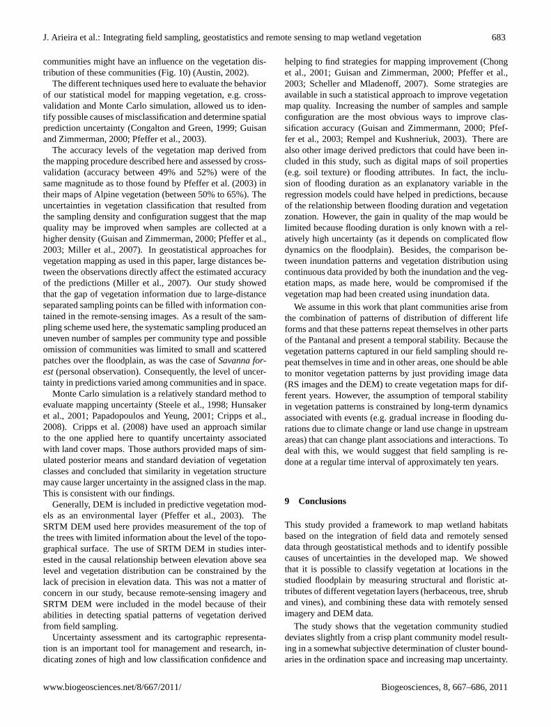
The relationship between vegetation distribution and flood-ing was assessed by comparing the plant community mapwith a flood duration map as in direct gradient analysis. Theflood duration map (Fig. 9) was created from a digital ele-vation map and 38 yr of daily recordings of the water level



Fig. 8. Results of Monte Carlo simulation, using 1000 random sim-ulations. (A) The colors on the map indicate the vegetation classwith the highest probability of occurrence at a cell. A color gradi-ent is used to show the value of this highest probability;(B) mapsof two single random realizations, color scale is identical to Fig. 8.

in the River Cuiaba (Fig. 1b) provided by the Brazilian Na-tional Water Agency (ANA;http://hidroweb.ana.gov.br). The40-m resolution digital elevation map was created with uni-versal kriging from 81 GPS elevation measurements at thesite and using SRTM DEM as an auxiliary variable (Valeri-ano and Abdon, 2007). A base station was installed for in-creased precision of the GPS measurements. Flood durationand flood depth data were also monitored by direct readingof staff gauges for two years (2007–2008) at the 23 samplingtransects. The relationship between flooding and elevationdata was tested with Pearson’s correlation coefficient. Statis-tically significant and strong correlations were found among

0

200

400

600

800

1000

Cuiabá River (Porto Cercado)

wetter yearsdrier years

year1968 1973 1978 1983 1988 1993 1998 2003 2008

Flood duration (avg days/yr)

elevation (meter a.s.l.)

flo

od

du

rati

on

(days

yr

)-1

128 130 132 134 136

300

250

200

150

100

50

0

56 23’Wo56 18’W

o

A

16 46’So

N1km0

16 57’So

B

C

wa

ter

lev

el(c

m)

Fig. 9. (A) Map with average number of days flooded per year at thestudy site, calculated over the period 1969–2007;(B) relationshipbetween flood duration (days yr−1) and elevation of the soil surface(m a.s.l.) observed at the 23 study transects;(C) water level fluctu-ation in the River Cuiaba between 1969 and 2007. Vertical dottedlines indicate the occurrence of drier and wetter years.

them (r > 70%; P ≤ 0.05) indicating the possibility of cal-culating flooding duration values over the floodplain throughthe indirect relationship between river water depth and ele-vation. Flood duration of a cell was calculated by comparingthe water level in the river and the topographical elevation ofthe cell for each day as follows: if the elevation value at acell was lower than the water level in the river on a certainday, the cell was considered flooded that day. This approachignores spatial variation in water level associated with down-stream gradients in water level, local depressions containingwater that is only partially connected with the main river, andsurface water fed by groundwater. However, the effect ofthese processes is relatively small as indicated by additionalfield sampling with the staff gauges.

The flood duration map (Fig. 9) shows the number offlooded days per year in the study area. Flood duration dataextracted from this map were classified into monthly inter-vals and the distribution of the plant communities found inthe vegetation map along this flooding gradient was plottedin Fig. 10. Figure 10 shows that the zonation of plant com-munities along the floodplain is clearly related to the durationof inundation. Alluvial forest andDense savannaoccur in


http://hidroweb.ana.gov.br


areas with a flooding duration of less than two months.Mon-odominant forest, although occupying a high proportion ofthe highest areas, has the highest occurrence at intermediaryflooding conditions, with a flooding duration between twoand four months.Open savannais mostly found where flood-ing lasts for four to six months per year.Grasslandis foundunder almost the whole range of flooding durations, howeverwith peaks of occurrence in areas with a flooding durationbelow two months and between four and six months of inun-dation.Alluvial low forestis mostly situated at locations witha flooding duration between 6–8 months.Shrublanddomi-nates the areas with the highest flooding duration. Aboveeight months of flood duration, there is no suitable conditionfor tree species establishment and the landscape is occupiedmostly byShrubland, Open savannaandGrassland. The oc-currence of monodominant forest in the last flood durationclass might be associated with the coarse representation ofspatial variation in flood duration, illustrated in Fig. 9.

8 Discussion

Wetland mapping at scales suitable for conservation can belimited by the lack of temporally and spatially consistentdatasets. The present study identifies an efficient method-ological approaches to map and understand spatio-temporalpatterns of wetland vegetation of the Pantanal. We provide aframework to map wetland habitats based on the integrationof field data and remotely sensed data through geostatisticmethods and identify possible causes of vegetation zonation.

The vegetation in our study area shows complex spatialpatterns. The use of universal kriging for mapping is valuablebecause it allows combining remote-sensing information andspatially distributed field observations, taking into accountthe spatial dependence of the variation not explained by theremote-sensing data. Most other classification methods (e.g.,maximum likelihood) do not allow this level of sophisticationin using composite spatial information.

The plant communities described in an existing classifica-tion (Nunes da Cunha et al., 2006) could be identified as clus-ters in the ordination space, thanks to the floristic propertiesincluded in the analyses that differentiated structurally sim-ilar but floristically different plant communities. However,sometimes clusters showed overlap on a number of factoraxes and boundaries between clusters were not always accu-rate. Such overlap probably indicates the existence of grad-ual changes in vegetation (Brzeziecki et al., 1993), whichis not represented in our model with sharp boundaries be-tween vegetation communities. Thus, the vegetation com-munity studied deviates slightly from our crisp plant com-munity model. This had two implications for our analysis.One is the subjective determination of cluster boundaries inthe ordination space, particularly in cases where boundarieswere not crisp. The other is related to the interpretation ofthe uncertainty analysis. One of the causes of uncertainty

Fig. 10.Fraction of occupied sites by the seven identified communi-ties along the flood duration gradient. Flooding gradient is dividedin five flood classes representing number of flooded months.

of the mapped vegetation is the uncertainty in the assign-ment of an interpolated point to a cluster in the ordinationspace. Overlap of clusters in the ordination space may ac-tually represent transition zones between plant communities,and are related to intrinsic uncertainty in classification (seealso, Fortin et al., 2000; Hernandez-Stefanoni and Dupuy,2007). Potential misclassification in these zones appears asuncertainty on the interpolated crisp map, particular in ar-eas close to mapped boundaries between plant communities.However, even though we recognize that plant community isa spatial concept rather than a well-delimited entity (Austinand Smith, 1989), we believe that the abstract definition ofcrisp boundaries is needed to interpret space-time vegetationpatterns over large areas.

Our analysis of the causes of vegetation zonation on thefloodplain indicated that flood duration is an important de-terminant of plant community distribution in space, influ-encing spatial transitions between different plant communi-ties. Different mechanisms of tolerance to prolonged flood-ing evolved by species of a community (Parolin, 2009) mightbe related to vegetation zonation as it controls the expan-sion of different sets of plants (Damasceno-Junior et al.,2005). On the other hand, non-linear response of com-munities to the flood duration gradient, as was the casefor Grassland, indicates that interaction with neighboring



communities might have an influence on the vegetation dis-tribution of these communities (Fig. 10) (Austin, 2002).

The different techniques used here to evaluate the behaviorof our statistical model for mapping vegetation, e.g. cross-validation and Monte Carlo simulation, allowed us to iden-tify possible causes of misclassification and determine spatialprediction uncertainty (Congalton and Green, 1999; Guisanand Zimmerman, 2000; Pfeffer et al., 2003).

The accuracy levels of the vegetation map derived fromthe mapping procedure described here and assessed by cross-validation (accuracy between 49% and 52%) were of thesame magnitude as to those found by Pfeffer et al. (2003) intheir maps of Alpine vegetation (between 50% to 65%). Theuncertainties in vegetation classification that resulted fromthe sampling density and configuration suggest that the mapquality may be improved when samples are collected at ahigher density (Guisan and Zimmerman, 2000; Pfeffer et al.,2003; Miller et al., 2007). In geostatistical approaches forvegetation mapping as used in this paper, large distances be-tween the observations directly affect the estimated accuracyof the predictions (Miller et al., 2007). Our study showedthat the gap of vegetation information due to large-distanceseparated sampling points can be filled with information con-tained in the remote-sensing images. As a result of the sam-pling scheme used here, the systematic sampling produced anuneven number of samples per community type and possibleomission of communities was limited to small and scatteredpatches over the floodplain, as was the case ofSavanna for-est(personal observation). Consequently, the level of uncer-tainty in predictions varied among communities and in space.

Monte Carlo simulation is a relatively standard method toevaluate mapping uncertainty (Steele et al., 1998; Hunsakeret al., 2001; Papadopoulos and Yeung, 2001; Cripps et al.,2008). Cripps et al. (2008) have used an approach similarto the one applied here to quantify uncertainty associatedwith land cover maps. Those authors provided maps of sim-ulated posterior means and standard deviation of vegetationclasses and concluded that similarity in vegetation structuremay cause larger uncertainty in the assigned class in the map.This is consistent with our findings.

Generally, DEM is included in predictive vegetation mod-els as an environmental layer (Pfeffer et al., 2003). TheSRTM DEM used here provides measurement of the top ofthe trees with limited information about the level of the topo-graphical surface. The use of SRTM DEM in studies inter-ested in the causal relationship between elevation above sealevel and vegetation distribution can be constrained by thelack of precision in elevation data. This was not a matter ofconcern in our study, because remote-sensing imagery andSRTM DEM were included in the model because of theirabilities in detecting spatial patterns of vegetation derivedfrom field sampling.

Uncertainty assessment and its cartographic representa-tion is an important tool for management and research, in-dicating zones of high and low classification confidence and

helping to find strategies for mapping improvement (Chonget al., 2001; Guisan and Zimmerman, 2000; Pfeffer et al.,2003; Scheller and Mladenoff, 2007). Some strategies areavailable in such a statistical approach to improve vegetationmap quality. Increasing the number of samples and sampleconfiguration are the most obvious ways to improve clas-sification accuracy (Guisan and Zimmermann, 2000; Pfef-fer et al., 2003; Rempel and Kushneriuk, 2003). There arealso other image derived predictors that could have been in-cluded in this study, such as digital maps of soil properties(e.g. soil texture) or flooding attributes. In fact, the inclu-sion of flooding duration as an explanatory variable in theregression models could have helped in predictions, becauseof the relationship between flooding duration and vegetationzonation. However, the gain in quality of the map would belimited because flooding duration is only known with a rel-atively high uncertainty (as it depends on complicated flowdynamics on the floodplain). Besides, the comparison be-tween inundation patterns and vegetation distribution usingcontinuous data provided by both the inundation and the veg-etation maps, as made here, would be compromised if thevegetation map had been created using inundation data.

We assume in this work that plant communities arise fromthe combination of patterns of distribution of different lifeforms and that these patterns repeat themselves in other partsof the Pantanal and present a temporal stability. Because thevegetation patterns captured in our field sampling should re-peat themselves in time and in other areas, one should be ableto monitor vegetation patterns by just providing image data(RS images and the DEM) to create vegetation maps for dif-ferent years. However, the assumption of temporal stabilityin vegetation patterns is constrained by long-term dynamicsassociated with events (e.g. gradual increase in flooding du-rations due to climate change or land use change in upstreamareas) that can change plant associations and interactions. Todeal with this, we would suggest that field sampling is re-done at a regular time interval of approximately ten years.

9 Conclusions

This study provided a framework to map wetland habitatsbased on the integration of field data and remotely senseddata through geostatistical methods and to identify possiblecauses of uncertainties in the developed map. We showedthat it is possible to classify vegetation at locations in thestudied floodplain by measuring structural and floristic at-tributes of different vegetation layers (herbaceous, tree, shruband vines), and combining these data with remotely sensedimagery and DEM data.

The study shows that the vegetation community studieddeviates slightly from a crisp plant community model result-ing in a somewhat subjective determination of cluster bound-aries in the ordination space and increasing map uncertainty.



We conclude that spatial patterns of vegetation distribu-tion in the studied floodplain is to a great extent determinedby the spatial patterns in inundation, as stressed by a num-ber of other studies in the Pantanal (Junk, 1989; Nunes daCunha and Junk, 1999, 2000; Zeilhofer and Schessl, 2000).In addition, patterns in vegetation are determined by spatialdependence in biological processes, such as competition be-tween neighbors and dispersal strategies (Tilman, 1994).

The cartographic representation of classification uncer-tainty gave useful information on the spatial distributionand sources of uncertainty. The simulation and the cross-validation results showed that uncertainty in classificationvaried in space and among communities, partly due to thesampling configuration. To avoid bias in sampling and re-sulting problems of omission of communities in the mappedarea, we suggest the use of stratified random samplingmethod or stratified systematic unaligned sampling in futurestudies (Lo and Watson, 1998). The inclusion of other re-motely sensed images in the model as a strategy for map im-provement needs to be taken into account in future studiesalso.

The significant advantage of the mapping approach de-scribed in this paper is that detailed biological informationfrom field observations can be integrated with high spatialresolution remotely sensed data producing accurate maps.Unlike “classical” approaches to vegetation class mapping,our modeling carries quantitative information on vegetationvariability and can be used to map vegetation over large ar-eas. We believe that mapping of plant communities by inte-grating field observations and high-resolution imagery usinggeostatistics is a promising approach for conservation assess-ment and long-term ecological monitoring in extensive wet-land areas.

Acknowledgements.The authors are grateful to the Braziliangovernmental agencies, CAPES and CNPq, for the financialsupport. Helpful comments and assistance were provided by FionaCarswell, P. Girard, Peter Zeihofer, Arnildo Pott, Vali J. Pott,Sandra Santos and Jose F. M. Valls. We also thank the SocialService of the Commerce (SESC) and technicians and students ofthe Federal University of Mato Grosso, for the technical supportin field work. Two anonymous reviewers are thanked for theirconstructive comments.

Edited by: F. Carswell

References

Ab’Saber, A. N.: O Pantanal Matogrossense e a teoria dos refugios,Rev. Bras. Geog., 50, 9–57, 1988.

Alvarenga, S. M., Brasil, A. E., Pinheiro, R., and Kux, H.J. H.: Estudo geomorfologico aplicadoa Bacia do alto RioParaguai e Pantanais Matogrossenses, Boletim Tecnico ProjetoRADAM/BRASIL, Serie Geomorfologia, Salvador, 187, 89–183, 1984.

Assine, M. L. and Soares, P. C.: Quaternary of the Pantanal, west-central Brazil, Quatern. Int., 114, 23–34, 2004.

Austin, M. P.: Spatial prediction of species distribution: an inter-face between ecological theory and statistical modelling, Ecol.Model., 157, 101–118, 2002.

Austin, M. P. and Smith, T. M.: A new model for the continuumconcept, Vegetatio, 83, 35–47, 1989.

Barbosa, R. I. and Ferreira, C. A. C.: Biomassa acima do solo deum ecossistema de “campina” em Roraima, norte da AmazoniaBrasileira, Acta Amazon., 34, 577–586, 2004.

Bascompte, J. and Sole, R. V.: Habitat fragmentation and extinctionthresholds in spatially explicit models, J. Anim. Ecol., 65, 465—473, 1996.

Bourennane, H., King, D., Couturier, A., Nicoullaud, B., Mary,B., and Richard, G.: Uncertainty assessment of soil water con-tent spatial patterns using geostatistical simulations: an empiricalcomparison of a simulation accounting for single attribute and asimulation accounting for secondary information, Ecol. Model.,205, 323–335, 2007.

Bowen, H. S.: Absolute radiometric calibration of the IKONOSsensor using radiometrically characterized stellar sources, in:Proceedings of the ISPRS Commission I Mid-Term Sympo-sium/Pecora 15-Land Satellite Information IV Conference, 10–14 November, Denver, CO, 2002.

Bray, J. R. and Curtis, J. T.: An ordination of the upland forestcommunities of southern Wisconsin, Ecol. Monogr., 27, 325–349, 1957.

Brzeziecki, B., Kienast, F., and Wildi, O.: A simulated map of thepotential natural forest vegetation of Switzerland, J. Veg. Sci., 4,499–508, 1993.

Bullock, J.: Plants, in: Ecological census techniques: a handbook,edited by: Sutherland, W. J., Cambridge Univ. Press, NY, 111–138, 1996.

Chambers, J. Q., Asner, G. P., Morton, D. C., Morton, D. C., An-derson, L. O., Saatchi, S. S., Espırito-Santo, F. D. B., and SouzaJr., M. P. C.: Regional ecosystem structure and function: eco-logical insights from remote sensing of tropical forests, TrendsEcol. Evol., 22, 414–423, 2007.

Chave, J., Andalo, C., Brown, S., Cairns, M. A., Chambers, J. Q.,Eamus, D., Folster, H., Fromard, F., Higuchi, N., Kira, T., Les-cure, J. P., Nelson, B. W., Ogawa, H., Puig, H., Riera, B., andYamakura, T.: Tree allometry and improved estimation of car-bon stocks and balance in tropical forests, Oecologia, 145, 87–99, 2005.

Chong, G. W., Reich, R. M., Kalkhan, M. A., and Stohlgren, T.J.: New approaches for sampling and modeling native and exoticplant species richness, West. N. Am. Naturalist, 61, 328–335,2001.

Colasanti, R. L., Hunt, R., and Watrud, L.: A simple cellular au-tomaton model for high-level vegetation dynamics, Ecol. Model.,203, 363–374, 2007.

Congalton, R. G. and Green, K.: Assessing the accuracy of remotelysensed data: principle and practices, Lewis Publishers, BocaRa-ton, USA, 1999.

Connell, J. H. and Slatyer, R. O.: Mechanisms of succession innatural communities and their role in community stability andorganization, Am. Nat., 111, 1119–1144, 1977.

Cripps, E., O’Hagan, A., Quaife, T., and Anderson, C. W.: Mod-elling uncertainty in satellite derived land cover maps, Research



Report No. 573/08, Department of Probability and Statistics,University of Sheffield, 2008.

Damasceno-Junior, G. A., Semir, J., Santos, F. A. M., and Leitao-Filho, H. F.: Structure, distribution of species and inundation ina riparian forest of Rio Paraguai, Pantanal, Brazil, Flora, 200,119–135, 2005.

De Musis, C. R., Junior, J. H. C., and Filho, N. P.: Caracterizacaoclimatologica da Bacia do Alto Paraguai, Geografia, 22, 5–21,1997.

Draper, N. R. and Smith, H.: Applied Regression Analysis, JohnWiley & Sons, Inc., New York, USA, 1998.

Efron, B. and Tibshirani, R.: Bootstrap methods for standard errors,confidence intervals, and other measures of statistical accuracy,Stat. Sci., 1, 54–75, 1986.

ESRI: Arc GIS, Version 9, Redlands, California, USA, 2006.Ferrier, S., Drielsma, M., Manion, G., and Watson, G.: Extended

statistical approaches to modelling spatial pattern in biodiversityin northeast New South Wales, II. Community-level modelling,Biodivers. Conserv., 11, 2309–2338, 2002.

Fortin, M.-J., Olson, R. J., Ferson, S., Iverson, L., Hunsaker, C., Ed-wards, G., Levine, D., Butera, K., and Klemas, V.: Issues relatedto the detection of boundaries, Landscape Ecol., 15, 453–466,2000.

Gardner, R. H. and Engelhardt, K. A. M.: Spatial processesthat maintain biodiversity in plant communities, Perspect. PlantEcol., 9, 211–228, 2008.

Grime, J. P.: Plant Strategies and Vegetation Processes, John Wiley& Sons, New York, USA, 1979.

Guisan, A. and Zimmermann, N. E.: Predictive habitat distributionmodels in ecology, Ecol. Model., 135, 147–186, 2000.

Hernandez-Stefanoni, J. L. and Dupuy, J. M.: Mapping species den-sity of trees, shrubs and vines in a tropical forest, using fieldmeasurements, satellite multiespectral imagery and spatial inter-polation, Biodivers. Conserv., 16, 3817–3833, 2007.

Hiemstra, P. H., Pebesma, E. J., Twenhofel, C. J. W., and Heuvelink,G. B. M.: Real-time automatic interpolation of ambient gammadose rates from the Dutch Radioactivity Monitoring Network,Comput. Geosci., 35, 1711–1721, 2008.

Hofmann, M., Gatu, C., and Kontoghiorghes, E. J.: Efficient algo-rithms for computing the best subset regression models for large-scale problems, Comput. Stat. Data An., 52, 16–29, 2007.

Hunsaker, C. T., Goodchild, M. F., and Friedl, M. A. (Eds.): Im-plications for Remote Sensing and GIS applications, Springer-Verlag New York, NY, 402 pp., 2001.

Jacobsen, K.: SRTM Height Models, in: GEOconnexion Interna-tional Magazine – Spatial data & landuse, edited by: Thurston,J. and Mai, W., UK, 5, 20–21, 2006.

James, F. C. and McCulloch, C. E.: Multivariate analysis in ecologyand systematics: panacea or pandora’s box?, Annu. Rev. Ecol.Syst., 21, 129–166, 1990.

Jensen, J. R.: Remote Sensing of the Environment – an Earth Re-source Perspective, 2nd edn., Upper Saddle River: Prentice-Hall,2007.

Jongman, R. H. G., ter Braak, C. J. F., and Van Togeren, O. F.R.: Data Analysis in Community and Landscape Ecology, Cam-bridge at the University press, Cambridge, UK, 1995.

Junk, W. J.: Flood tolerance and tree distribution in central Amazo-nian floodplains, in: Tropical Forests: Botanical Dynamics, Spe-ciation and Diversity, edited by: Haynes, R. R., Holm-Nielsen,

L. B., and Balslev, H., Academic Press, London, 47–64, 1989.Junk, W. J.: Long-term environmental trends and the future of trop-

ical wetlands, Environ. Conserv., 29, 414–435, 2002.Junk, W. J., Bayley, P. B., and Sparks, R. E.: The flood pulse con-

cept in river-floodplain systems, in: Proceedings of the Interna-tional Large River Symposium, Canadian Special Publication ofFisheries and Aquatic Sciences, edited by: Dodge, D. P., Ottawa,Canada, 110–127, 1989.

Junk, W. J., Nunes da Cunha, C., Wantzen, K. M., Petermann, P.,Strussmann, C., Marques, M. I., and Adis, J.: Biodiversity andits conservation in the Pantanal of Mato Grosso, Brazil, Aquat.Sci., 68, 278–309, 2006.

Koppen, W.: Climatologia, Fondo de Cultura, Buenos Aires, Ar-gentina, 1948.

Legendre, P. and Legendre, L.: Numerical Ecology, Elsevier, Ams-terdam, 1998.

Lo, C. P. and Watson, L. J.: The influence of geographic samplingmethods on vegetation map accuracy evaluation in a swampy en-vironment, Photogramm. Eng. Rem. S., 64, 1189–1200, 1998.

Magnusson, W. E., Lim, A. P, Luizao, R., Luizao, F., Costa, F. R. C.,Castilho, C. V., and Kinupp, V. F.: RAPELD: uma modificacaodo metodo de Gentry para inventario da biodiversidade em sıtiospara pesquisa ecologica de longa duracao, Biota Neotropica, 5,http://www.biotaneotropica.org.br/v5n2, 2005.

Mallows, C. L.: Some Comments onCp, Technometrics, 15, 661–675, 1973.

McIntosh, R. P.: Plant Communities, Science, 128, 115–120, 1958.Minchin, P. R.: Montane vegetation of the Mt. Field Massif, Tas-

mania: a test of some hypotheses about properties of communitypatterns, Plant Ecol., 83, 97–110, 1989.

Miller, J., Franklin, J., and Aspinall, R.: Incorporating spatial de-pendence in predictive vegetation models, Ecol. Model., 202,225–242, 2007.

Mitsch, W. J., Gosselink, J. G., Anderson, C. J., and Zhang, L.:Wetland Ecosystems, John Wiley & Sons, Inc., New York, 2009.

Nunes da Cunha, C. and Junk, W. J.: Composicao florıstica decapoes e cordilheiras: localizacao das especies lenhosas quantoao gradiente de inundacao no Pantanal de Pocone, MT, Brasil,in: Anais do II Simposio sobre Recursos Naturais e Socio-Economicos do Pantanal – Manejo e Conservacao, Embrapa –CPAP, Corumba, Brasil, 387–406, 1999.

Nunes da Cunha, C. and Junk, W. J.: The impact of floodingon distribution of woody plant communities in the Pantanal ofPocone, Mato Grosso, Brazil, in: German-Brazilian Workshopon Neotropical Ecosystems – Achievements and Prospects of Co-operative Research, Session 4: Living Resource Management:Approaches, Techniques, Variability, Hamburg, Germany, 3–8,2000.

Nunes da Cunha, C., Rawiel, P., Wantzen, K. M., Junk, W. J., andPrado, A. L.: Mapping and characterization of vegetation unitsby means of Landsat imagery and management recommenda-tions for the Pantanal of Mato Grosso (Brazil), north of Pocone,Amazoniana, XIX, 1–32, 2006.

Papadopoulos, C. E. and Yeung, H.: Uncertainty estimation andMonte Carlo simulation method, Flow Meas. Instrum., 12, 291–298, 2001.

Pardo-Iguzquiza, E. and Chica-Olmo, M.: Geostatistics with theMatern semivariogram model: a library of computer programsfor inference, kriging and simulation, Comput. Geosci., 34,


http://www.biotaneotropica.org.br/v5n2


1073–1079, 2008.Parolin, P.: Submerged in darkness: adaptations to prolonged sub-

mergence by woody species of the Amazonian floodplains, Ann.Bot., 103, 359–376, 2009.

PCRaster: PCRaster Software, info at:http://pcraster.geo.uu.nl/,2002.

Pebesma, E. J. and Wesseling, C. G.: GSTAT: a program for geosta-tistical modelling, prediction and simulation, Comput. Geosci.,24, 17–31, 1998.

Pfeffer, K., Pebesma, E. J., and Burrough, P. A.: Mapping alpinevegetation using vegetation observations and topographic at-tributes, Landscape Ecol., 18, 759–776, 2003.

Pillar, V. D. and Sosinski Jr., E. E.: An improved method for search-ing plant functional types by numerical analysis, J. Veg. Sci., 14,323–332, 2003.

R Development Core Team: R: A Language and Environment forStatistical Computing, R Foundation for Statistical Computing,Vienna, Austria, ISBN-3-900051-07-0,http://www.R-project.org, 2009.

Rempel, R. S. and Kushneriuk, R. S.: The influence of samplingscheme and interpolation method on the power to detect spatialeffects of forest birds in Ontario (Canada), Landscape Ecol., 18,741–757, 2003.

Scheller, R. and Mladenoff, D.: An ecological classification of for-est landscape simulation models: tools and strategies for under-standing broad-scale forested ecosystems, Landscape Ecol., 22,491–505, 2007.

Schongart, J., Arieira, J., Felfili Fortes, C., Cezarine de Arruda,E., and Nunes da Cunha, C.: Carbon dynamics in above-ground coarse wood biomass of wetland forests in the north-ern Pantanal, Brazil, Biogeosciences Discuss., 5, 2103–2130,doi:10.5194/bgd-5-2103-2008, 2008.

Silva, M. P., Mauro, R., Mourao, G. E., and Coutinho, M.:Distribuicao e quantificacao de classes de vegetacao do Pantanalatraves de levantamento aereo, Rev. Bras. Bot., 23, 143–152,2000.

Steele, B. M., Winne, J. C., and Redmond, R. L.: Estimationand mapping of misclassification probabilities for thematic landcover maps, Remote Sens. Environ., 66(2), 192–202, 1998.

Stein, A. and Corsten, L. C. A.: Universal kriging and cokriging asa regression procedure, Biometrics, 47, 575–587, 1991.

Svenning, J. C., Kinner, D. A., Stallard, R. F., Engelbrecht, B. M.J., and Wright, S. J.: Ecological determinism in plant communitystructure across a tropical forest landscape, Ecology, 85, 2526–2538, 2004.

Tilman, D.: Plant Strategies and the Dynamic and Structure of PlantCommunities, Princeton University Press, Princeton, New Jer-sey, 1988.

Tilman, D.: Competition and biodiversity in spatially structuredhabitats, Ecology, 75, 2–16, 1994.

Tucker, C. J.: Red and photographic infrared linear combinationsfor monitoring vegetation, Remote Sens. Environ., 8, 127–150,1979.

Turner, M. G.: Landscape ecology: the effect of pattern on process,Annu. Rev. Ecol. Syst., 20, 171–197, 1989.

Turner, M. G., Gardner, R. H., and O’Neill, R. V.: Landscape Ecol-ogy in Theory and Practice- Pattern and Process, Springer-VerlagNew York, Inc., USA, 2001.

Valeriano, M. M. and Abdon, M. M.: Aplicacao de dados SRTM aestudos do Pantanal, Rev. Bras. Cartog., 59, 63–71, 2007.

Velloso, H. P., Rangel Filho, A. L. R., and Lima, J. C. A.:Classificacao da Vegetacao Brasileira Adaptada a um SistemaUniversal, IBGE, RJ, BR, 1991.

Wagner, H. H. and Fortin, M. J.: Spatial analysis of landscapes:concepts and statistics, Ecology, 86, 1975–1987, 2005.

Wantzen, K. M., Drago, E., and da Silva, C. J.: Aquatic habitatsof the Upper Paraguay River-Floodplain-System and parts of thePantanal (Brazil), Ecohydrol. Hydrobiol., 5, 107–126, 2005.

Wesseling, C. G., Karssenberg, D., Van Deursen, W. P. A., and Bur-rough, P. A.: Integrating dynamic environmental models in GIS:the development of a Dynamic Modelling language, Transactionsin GIS, 1, 40–48, 1996.

Whittaker, R. W.: Gradient analysis of vegetation, Biol. Rev., 49,207–264, 1967.

Zeilhofer, P. and Schessl, M.: Relationship between vegetationand environmental conditions in the northern Pantanal of MatoGrosso, J. Biogeogr., 27, 159–168, 2000.


http://pcraster.geo.uu.nl/

http://www.R-project.org

http://www.R-project.org

http://dx.doi.org/10.5194/bgd-5-2103-2008

Integrating ﬁeld sampling, geostatistics and remote ... · J. Arieira et al.: Integrating ﬁeld...

Documents

Transcript of Integrating ﬁeld sampling, geostatistics and remote ... · J. Arieira et al.: Integrating ﬁeld...