i

Integrated Waterbird Management and Monitoring Approach

for Nonbreeding Waterbirds

Monitoring Manual Version 8: February 2015

Scrub-shrub Mallards. Photo Credit: Mick Hanan FWS

2

INTRODUCTION

The Challenge - Sustaining healthy populations of waterbirds that migrate long distances is a major

challenge for land managers. How does a manager know which species to manage for at a specific

site? How important is a single site in the big picture? How can many managers coordinate their

management of impoundments across the landscape so that the birds have the right amount and

quality of habitat, at the right time, in the right places? As part of the IWMM approach, managers

and scientists are working together to develop integrated monitoring protocols, decision support

models, and a database that will inform waterbird management decisions at multiple spatial scales.

These products will support clear and transparent decision making processes with respect to

waterbird habitat management.

The Integrated Waterbird Management and Monitoring (IWMM) approach was initiated by

conducting structured decision-making (SDM) workshops to develop an operational framework for

management and monitoring of waterfowl, shorebirds, and wading birds, collectively referred to as

waterbirds, at the local, regional and flyway spatial scales (Coppen et al. 2007, Laskowski et al.

2008, Lor et al. 2008). Through these workshops IWMM developed a multi-scaled adaptive

management process that will inform local, regional/state, and flyway managers about how they can

best meet the needs of migrating and wintering waterbird populations. Waterbird needs during the

migration and winter phases of their life-cycle are just as critical as those during the breeding

season. However, IWMM is the only landscape scale monitoring effort developed to date that

tracks and links waterbird habitat use, habitat conditions and management actions during the

migration and wintering periods. This approach includes a monitoring component that assesses how

well managers at all scales are meeting their management objectives and an adaptive feedback loop

that allows managers to adjust their management to address emerging threats.

This manual provides survey techniques (i.e. procedures) described herein that involve visual

assessments of whole-wetland unit habitat conditions and counts of waterbirds conducted from the

perimeter of the wetland unit. A series of standard operating procedures provides greater detail on

recommended methods and technical aspects of this protocol, and were used to develop a national

protocol framework to guide the local monitoring component of the IWMM approach at units

within the National Wildlife Refuge System. Data entry, archival, and multi-scale analysis are

handled through an online database that is part of the Avian Knowledge Network.

Refer to the following for the complete protocol framework:

Loges BW, Tavernia BG, Wilson AM, Stanton JD, Herner-Thogmartin JH, Casey J, Coluccy JM,

Coppen JL, Hanan M, Heglund PJ, Jacobi SK, Jones T, Knutson MG, Koch KE, Lonsdorf EV,

Laskowski HP, Lor SK, Lyons JE, Seamans ME, Stanton W, Winn B, and Ziemba LC. 2014.

National protocol framework for the inventory and monitoring of nonbreeding waterbirds and their

habitats, an Integrated Waterbird Management and Monitoring Initiative (IWMM) approach.

Natural Resources Program Center, Fort Collins, CO. This protocol is available from ServCat:

[http://ecos.fws.gov/ServCatFiles/Reference/Holding/40340]

3

Why Monitor Waterbirds and their Habitats?

We anticipate that setting and obtaining local management objectives will require knowledge about

waterbird use, setting habitat condition objectives, the ability to assess the efficacy of management

actions (e.g. accounting for management costs in terms of use-days or supported populations), and /

or the ability to learn how to improve management (Lyons et al. 2008). Also, depending on the

management objective, the survey activity will often entail assessing status and trends of habitat

conditions or waterbird numbers. Resulting data may be used to calculate wetland unit-specific

waterbird use-days, document migration chronologies, and explore relationships between waterbird

counts, management actions and habitat condition.

Survey Units

A survey unit is a single managed or unmanaged wetland unit. Boundaries of the unit should be

fixed throughout the season and across years to ensure data comparability. See Standard Operating

Procedure (SOP 1).

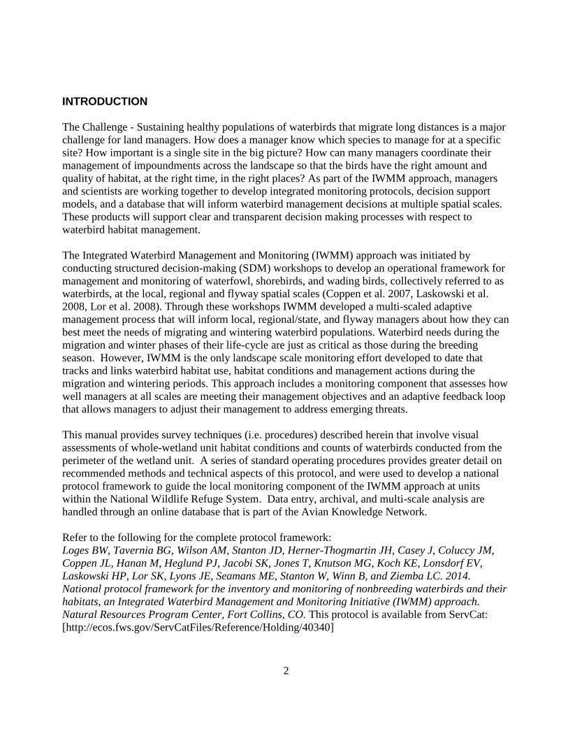
Site, survey unit, and observer codes will be assigned by IWMM staff to ensure that they do not

duplicate codes in use by other

cooperators. Please contact the Science

Coordinator

(iwmmprogram@gmail.com) for

assistance in assigning codes. If you do

not know the codes, please leave them

blank, but make sure that you fill in

name details so that the codes can be

completed subsequently. Please refer to

SOPs 2 - 5 for additional information

regarding pre-survey logistics and

preparation, including equipment

needed for waterbird and vegetation

surveys.

Survey timing and schedule

Waterbird and unit condition surveys are completed weekly or biweekly during the non-breeding

waterbird season. See SOP 2.

4

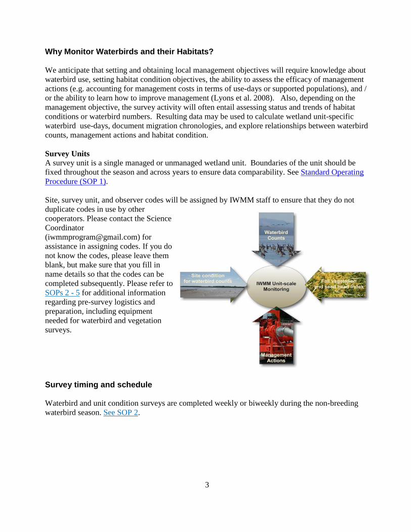
Figure 1. Generalized annual schedule for the Midwest for implementing waterfowl surveys,

vegetation surveys, data entry, and reporting. Flexibility in assigning start and end dates for key

tasks has been retained to facilitate customization of site-specific protocols.

A practical approach for selecting survey dates during the non-breeding season is to systematically

conduct Waterbird and Unit Condition Surveys on a weekly or biweekly basis. Subjective selection of

survey dates should be avoided because it can introduce bias into migration curves and bird use-day

estimates.

Vegetation surveys are completed once late in the growing season. See SOP 5.

Recording Management Activities. In addition to monitoring waterbird use and habitat

response, routine short-term habitat management activities from the start of the current year’s

growing season to the start of the next year’s growing season will be tracked for each management

unit. See SOP 6.

Data entry The IWMM will be transitioning to an online database that will be part of the Avian Knowledge

Network (AKN). This database will provide centralized data entry and reporting capabilities for

IWMM cooperators. As a member of the AKN, IWMM will be able to share data and tools with

other members, such as the International Shorebird Survey. Cooperators should enter collected data

into the IWMM’s centralized, online database. More specific instructions for entering data into this

database can be found in SOP 7.

5

Qualifications All surveys need to be conducted by qualified individuals. Surveyors should be able to:

• Identify waterbird species

• Identify common wetland plant species

• Estimate numbers of waterbirds using advocated techniques

• Follow survey protocols

Training Cooperators should visit the IWMM website at: http://iwmmprogram.ning.com/ for a 20-minute

webinar that will introduce IWMM and its waterbird and vegetation survey methods. This webinar

can be found on the Presentations page as IWMM Training Presentation 2012. Updates are

presently being made for the 2015 season. Inexperienced waterbird counters are advised to practice

their counting and estimation techniques before participating in IWMM.

Data collectors should also be trained for dealing with any local hazards and proper procedures for

handling and collecting injured or dead wildlife. For instructions on how to handle and submit

waterfowl carcasses for cause of death diagnosis, please see Supplemental Materials (SM-8) as well

as the Mortality Event Response instructions on the Wildlife Health office internal website:

https://sites.google.com/a/fws.gov/fws-wildlife-health/products.

Please use the Q&A forum within the website for general methodological queries. Alternatively,

use the messaging feature to contact the Science Coordinator. To access the Q&A forum or

messaging features, you will need a membership, email iwmmprogram@gmail.com.

Dead birds If carcasses of waterbirds are found, follow the guidelines provided in SM 8.

For More Information:

o IWMM National Project Coordinator—Linda Wires USFWS, 5600 American Blvd West,

Bloomington, MN 55427 Linda_wires@fws.gov

o IWMM National Science Coordinator—Tim Jones (Interim) USFWS, Merriam Lab, Room

215 11510 American Holly Drive Laurel, MD 20708. iwmmprogram@gmail.com

o Midwest- Brian Loges, Two Rivers National Wildlife Refuge, HC 82 Box 107 Brussels, IL.

Brian_Loges@fws.gov

o Southeast & Northeast- John Stanton, U.S. Fish and Wildlife Service, North Carolina

Migratory Bird Field Office, 155 L.A. Keiser Drive, Suite A, Columbia, North Carolina

27925. John_Stanton@fws.gov

6

SOP 1: Delineating Unit Boundaries

Before conducting waterbird and vegetation surveys, follow these instructions to delineate the

boundaries of each unit surveyed. Once boundaries are established for a unit those boundaries

should remain the same throughout the season and year to year. Equipment

GPS

Printed aerial images

GIS & digital imagery

Observers should define survey unit boundaries to accommodate whole-area waterbird counts and

vegetation surveys. On managed lands, wetlands are often divided into management units.

Wherever possible, existing management units will be used as survey units. A management unit is

defined as a fixed area where recurring waterbird management actions are applied. Management

actions may vary in type and frequency. Cooperators have the discretion to survey units ranging

from intensively managed moist-soil systems to protected natural wetlands with no habitat

manipulation.

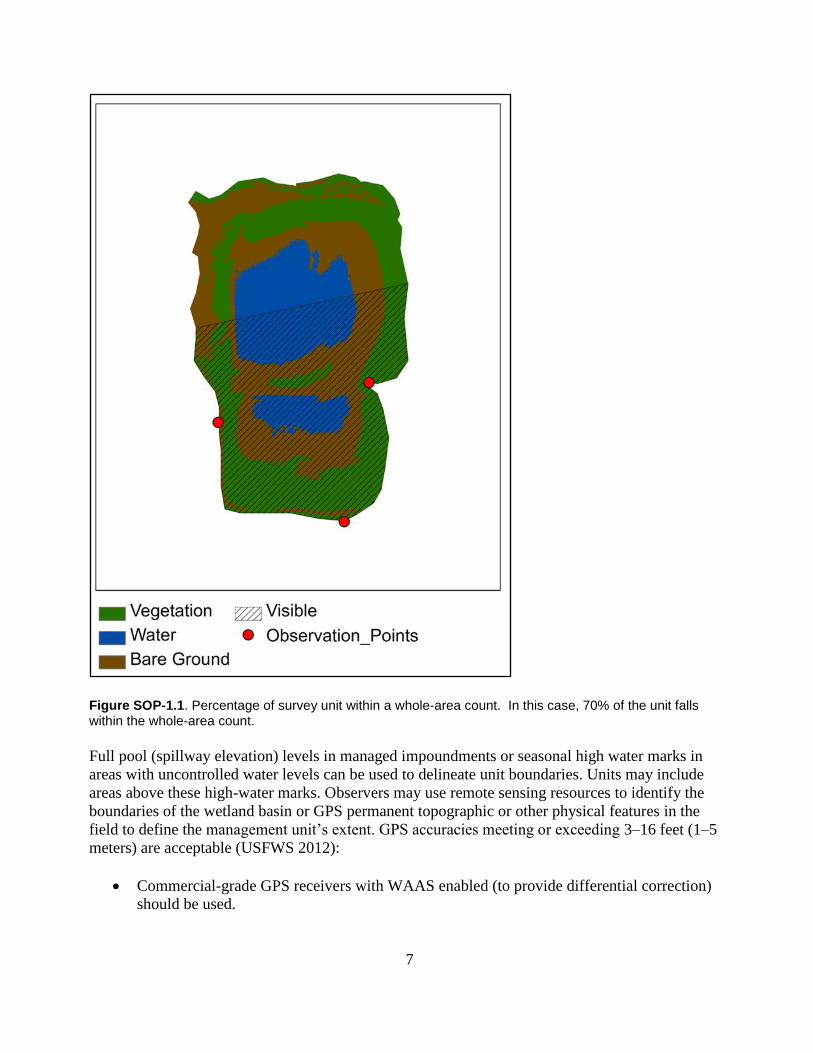
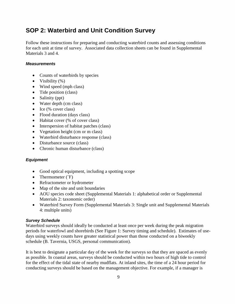
It is expected that the observer will be able to visually assess >70% of the survey/management unit

(Figure SOP-1.1). If an observer cannot visually assess >70% of a unit’s area, additional vantage

points should be added in lieu of splitting the management unit into multiple survey units. This

criterion applies to the surface area of a unit not to the visibility of birds within a unit. While

multiple observation points can be established around the perimeter of the unit to meet this

criterion, but observers should bear in mind the need to complete the count on the unit within a

single morning and to minimize multiple counting of individual birds. Note that the boundaries of

the unit should be fixed through the season and across years to ensure data comparability.

7

Figure SOP-1.1. Percentage of survey unit within a whole-area count. In this case, 70% of the unit falls within the whole-area count.

Full pool (spillway elevation) levels in managed impoundments or seasonal high water marks in

areas with uncontrolled water levels can be used to delineate unit boundaries. Units may include

areas above these high-water marks. Observers may use remote sensing resources to identify the

boundaries of the wetland basin or GPS permanent topographic or other physical features in the

field to define the management unit’s extent. GPS accuracies meeting or exceeding 3–16 feet (1–5

meters) are acceptable (USFWS 2012):

Commercial-grade GPS receivers with WAAS enabled (to provide differential correction)

should be used.

8

Relatively inexpensive GPS receivers or hand-held (cell phones) devices do not provide the

needed 3–16 feet meter accuracy.

Position averaging is recommended to meet the accuracy requirement.

Metadata should reflect estimated accuracies from field personnel during data collection

activities.

To facilitate inter-year comparisons of observations, survey unit boundaries should not be altered.

Observers should create and maintain printed maps and geospatial layers as aids in maintaining

consistent boundaries.

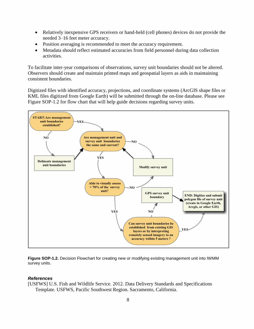
Digitized files with identified accuracy, projections, and coordinate systems (ArcGIS shape files or

KML files digitized from Google Earth) will be submitted through the on-line database. Please see

Figure SOP-1.2 for flow chart that will help guide decisions regarding survey units.

Figure SOP-1.2. Decision Flowchart for creating new or modifying existing management unit into IWMM survey units.

References

[USFWS] U.S. Fish and Wildlife Service. 2012. Data Delivery Standards and Specifications

Template. USFWS, Pacific Southwest Region. Sacramento, California.

9

SOP 2: Waterbird and Unit Condition Survey Follow these instructions for preparing and conducting waterbird counts and assessing conditions

for each unit at time of survey. Associated data collection sheets can be found in Supplemental

Materials 3 and 4.

Measurements

Counts of waterbirds by species

Visibility (%)

Wind speed (mph class)

Tide position (class)

Salinity (ppt)

Water depth (cm class)

Ice (% cover class)

Flood duration (days class)

Habitat cover (% of cover class)

Interspersion of habitat patches (class)

Vegetation height (cm or m class)

Waterbird disturbance response (class)

Disturbance source (class)

Chronic human disturbance (class)

Equipment

Good optical equipment, including a spotting scope

Thermometer (˚F)

Refractometer or hydrometer

Map of the site and unit boundaries

AOU species code sheet (Supplemental Materials 1: alphabetical order or Supplemental

Materials 2: taxonomic order)

Waterbird Survey Form (Supplemental Materials 3: Single unit and Supplemental Materials

4: multiple units)

Survey Schedule

Waterbird surveys should ideally be conducted at least once per week during the peak migration

periods for waterfowl and shorebirds (See Figure 1: Survey timing and schedule). Estimates of use-

days using weekly counts have greater statistical power than those conducted on a biweekly

schedule (B. Tavernia, USGS, personal communication).

It is best to designate a particular day of the week for the surveys so that they are spaced as evenly

as possible. In coastal areas, surveys should be conducted within two hours of high tide to control

for the effect of the tidal state of nearby mudflats. At inland sites, the time of a 24 hour period for

conducting surveys should be based on the management objective. For example, if a manager is

10

interested in supporting roosting activities, the counts should occur during a period when birds are

most likely to be roosting in a site. Flexibility in the timing of surveys is needed to address

constraints such as staffing, other activities taking place within units (e.g. hunting or management),

and weather.

If multiple units are surveyed, it is good practice to change the order of surveys by choosing

different starting units on each visit (wherever possible). If count numbers are expected to be

compiled, counts for all units should be completed in one day to minimize the interchange of birds

across units. Multiple-counting of individual waterbirds should be avoided. If birds regularly flush

from units during counts, then efforts to minimize disturbance during surveys or concurrent surveys

may be needed to minimize the multiple-counting of birds. Include waterbirds in the totals for only

the first unit in which you encounter them. Waterbirds observed outside the unit boundaries during

flood events, as flyovers or on adjacent dry land should not be included in the survey unit

observations.

There is no time limit for surveys. The observer should tally the waterbirds present when the

observation starts but should cease when there is a great deal of movement into the unit. Ideally, all

units within a site should be surveyed on the same day.

NOTE: During the waterfowl hunting season it is important to avoid conflict with hunting interests.

Disturbance can be avoided by surveying from accessible points around the perimeter of wetlands,

and by avoiding surveys when hunting activity is highest.

Site, unit and observer codes

Please contact the Science Coordinator (iwmmprogram@gmail.com) for assistance on assigning

codes. Site, survey unit, and observer codes must be assigned by IWMM staff to ensure that they do

not duplicate codes in use by other cooperators. If you do not know these codes, please leave them

blank, but make sure that you provide enough detail (e.g., name of observer, location of surveys) so

that the codes can be completed subsequently. Percent Visibility

To conduct whole-area counts, it is required that you be able to see >70% of the survey unit from

one or multiple vantage points placed around the unit’s perimeter. Estimate the percentage of the

survey unit included within the whole-area count (Figure SOP-2.1).

11

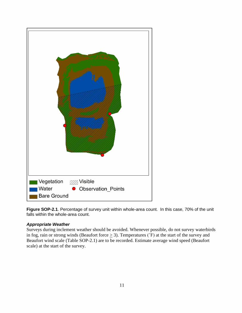
Figure SOP-2.1. Percentage of survey unit within whole-area count. In this case, 70% of the unit falls within the whole-area count. Appropriate Weather

Surveys during inclement weather should be avoided. Whenever possible, do not survey waterbirds

in fog, rain or strong winds (Beaufort force > 3). Temperatures (˚F) at the start of the survey and

Beaufort wind scale (Table SOP-2.1) are to be recorded. Estimate average wind speed (Beaufort

scale) at the start of the survey.

12

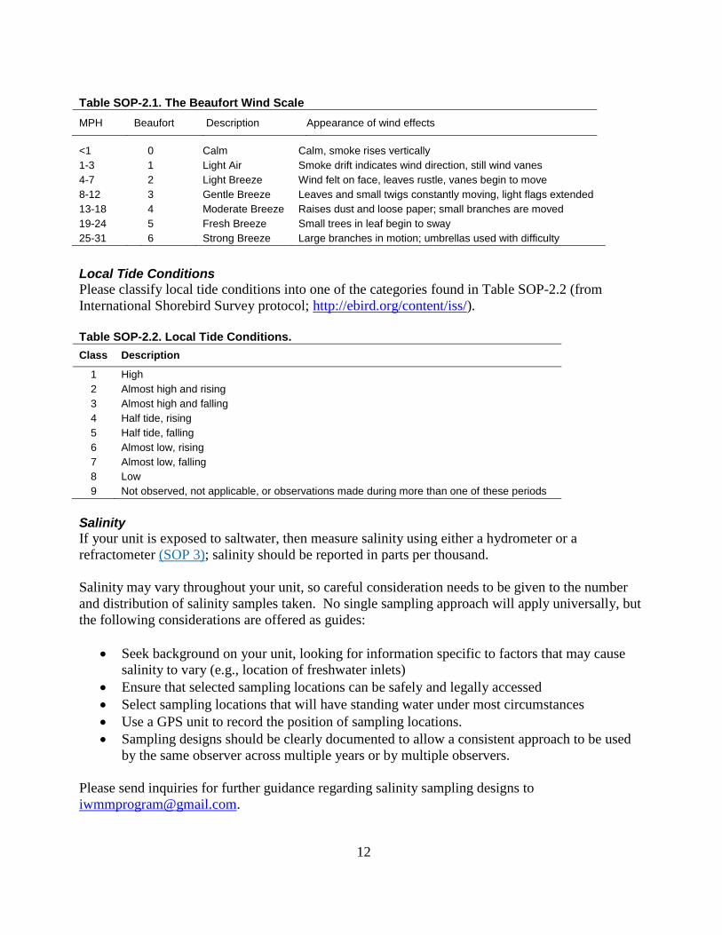
Table SOP-2.1. The Beaufort Wind Scale

MPH Beaufort Description Appearance of wind effects

Local Tide Conditions

Please classify local tide conditions into one of the categories found in Table SOP-2.2 (from

International Shorebird Survey protocol; http://ebird.org/content/iss/).

Table SOP-2.2. Local Tide Conditions.

Class Description

1 High

2 Almost high and rising

3 Almost high and falling

4 Half tide, rising

5 Half tide, falling

6 Almost low, rising

7 Almost low, falling

8 Low

9 Not observed, not applicable, or observations made during more than one of these periods

Salinity

If your unit is exposed to saltwater, then measure salinity using either a hydrometer or a

refractometer (SOP 3); salinity should be reported in parts per thousand.

Salinity may vary throughout your unit, so careful consideration needs to be given to the number

and distribution of salinity samples taken. No single sampling approach will apply universally, but

the following considerations are offered as guides:

Seek background on your unit, looking for information specific to factors that may cause

salinity to vary (e.g., location of freshwater inlets)

Ensure that selected sampling locations can be safely and legally accessed

Select sampling locations that will have standing water under most circumstances

Use a GPS unit to record the position of sampling locations.

Sampling designs should be clearly documented to allow a consistent approach to be used

by the same observer across multiple years or by multiple observers.

Please send inquiries for further guidance regarding salinity sampling designs to

iwmmprogram@gmail.com.

<1 0 Calm Calm, smoke rises vertically

1-3 1 Light Air Smoke drift indicates wind direction, still wind vanes

4-7 2 Light Breeze Wind felt on face, leaves rustle, vanes begin to move

8-12 3 Gentle Breeze Leaves and small twigs constantly moving, light flags extended

13-18 4 Moderate Breeze Raises dust and loose paper; small branches are moved

19-24 5 Fresh Breeze Small trees in leaf begin to sway

25-31 6 Strong Breeze Large branches in motion; umbrellas used with difficulty

13

If multiple samples are taken, report the mean value. If you do not take readings, report "NA". If

you are certain that the unit is never subject to saltwater incursion, report “< 0.5” (the numerical

definition of freshwater).

Water Gauge Reading

If the unit has a water level gauge, please record a reading each time a count is conducted. Be sure

to provide the measurement units of the water level gauge.

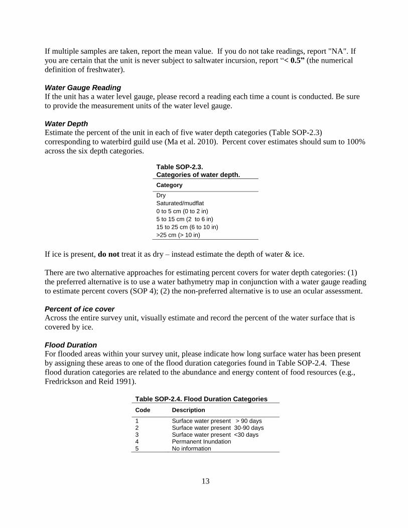
Water Depth

Estimate the percent of the unit in each of five water depth categories (Table SOP-2.3)

corresponding to waterbird guild use (Ma et al. 2010). Percent cover estimates should sum to 100%

across the six depth categories.

Table SOP-2.3. Categories of water depth.

Category

Dry

Saturated/mudflat

0 to 5 cm (0 to 2 in)

5 to 15 cm (2 to 6 in)

15 to 25 cm (6 to 10 in)

>25 cm (> 10 in)

If ice is present, do not treat it as dry – instead estimate the depth of water & ice.

There are two alternative approaches for estimating percent covers for water depth categories: (1)

the preferred alternative is to use a water bathymetry map in conjunction with a water gauge reading

to estimate percent covers (SOP 4); (2) the non-preferred alternative is to use an ocular assessment.

Percent of ice cover

Across the entire survey unit, visually estimate and record the percent of the water surface that is

covered by ice.

Flood Duration

For flooded areas within your survey unit, please indicate how long surface water has been present

by assigning these areas to one of the flood duration categories found in Table SOP-2.4. These

flood duration categories are related to the abundance and energy content of food resources (e.g.,

Fredrickson and Reid 1991).

Table SOP-2.4. Flood Duration Categories

Code Description

1 Surface water present > 90 days 2 Surface water present 30-90 days 3 Surface water present <30 days 4 Permanent Inundation 5 No information

14

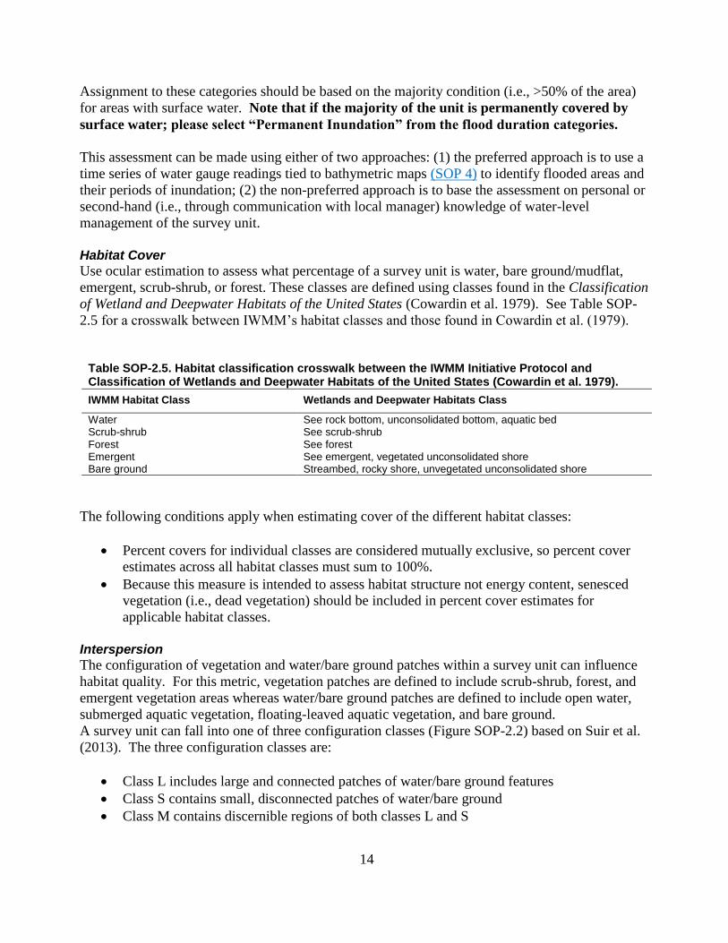
Assignment to these categories should be based on the majority condition (i.e., >50% of the area)

for areas with surface water. Note that if the majority of the unit is permanently covered by

surface water; please select “Permanent Inundation” from the flood duration categories.

This assessment can be made using either of two approaches: (1) the preferred approach is to use a

time series of water gauge readings tied to bathymetric maps (SOP 4) to identify flooded areas and

their periods of inundation; (2) the non-preferred approach is to base the assessment on personal or

second-hand (i.e., through communication with local manager) knowledge of water-level

management of the survey unit.

Habitat Cover

Use ocular estimation to assess what percentage of a survey unit is water, bare ground/mudflat,

emergent, scrub-shrub, or forest. These classes are defined using classes found in the Classification

of Wetland and Deepwater Habitats of the United States (Cowardin et al. 1979). See Table SOP-

2.5 for a crosswalk between IWMM’s habitat classes and those found in Cowardin et al. (1979).

Table SOP-2.5. Habitat classification crosswalk between the IWMM Initiative Protocol and Classification of Wetlands and Deepwater Habitats of the United States (Cowardin et al. 1979).

IWMM Habitat Class Wetlands and Deepwater Habitats Class

Water See rock bottom, unconsolidated bottom, aquatic bed

Scrub-shrub See scrub-shrub

Forest See forest Emergent See emergent, vegetated unconsolidated shore Bare ground Streambed, rocky shore, unvegetated unconsolidated shore

The following conditions apply when estimating cover of the different habitat classes:

Percent covers for individual classes are considered mutually exclusive, so percent cover

estimates across all habitat classes must sum to 100%.

Because this measure is intended to assess habitat structure not energy content, senesced

vegetation (i.e., dead vegetation) should be included in percent cover estimates for

applicable habitat classes.

Interspersion

The configuration of vegetation and water/bare ground patches within a survey unit can influence

habitat quality. For this metric, vegetation patches are defined to include scrub-shrub, forest, and

emergent vegetation areas whereas water/bare ground patches are defined to include open water,

submerged aquatic vegetation, floating-leaved aquatic vegetation, and bare ground.

A survey unit can fall into one of three configuration classes (Figure SOP-2.2) based on Suir et al.

(2013). The three configuration classes are:

Class L includes large and connected patches of water/bare ground features

Class S contains small, disconnected patches of water/bare ground

Class M contains discernible regions of both classes L and S

15

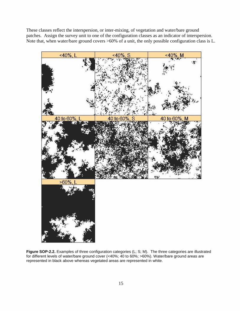
These classes reflect the interspersion, or inter-mixing, of vegetation and water/bare ground

patches. Assign the survey unit to one of the configuration classes as an indicator of interspersion.

Note that, when water/bare ground covers >60% of a unit, the only possible configuration class is L.

Figure SOP-2.2. Examples of three configuration categories (L; S; M). The three categories are illustrated for different levels of water/bare ground cover (<40%; 40 to 60%; >60%). Water/bare ground areas are represented in black above whereas vegetated areas are represented in white.

16

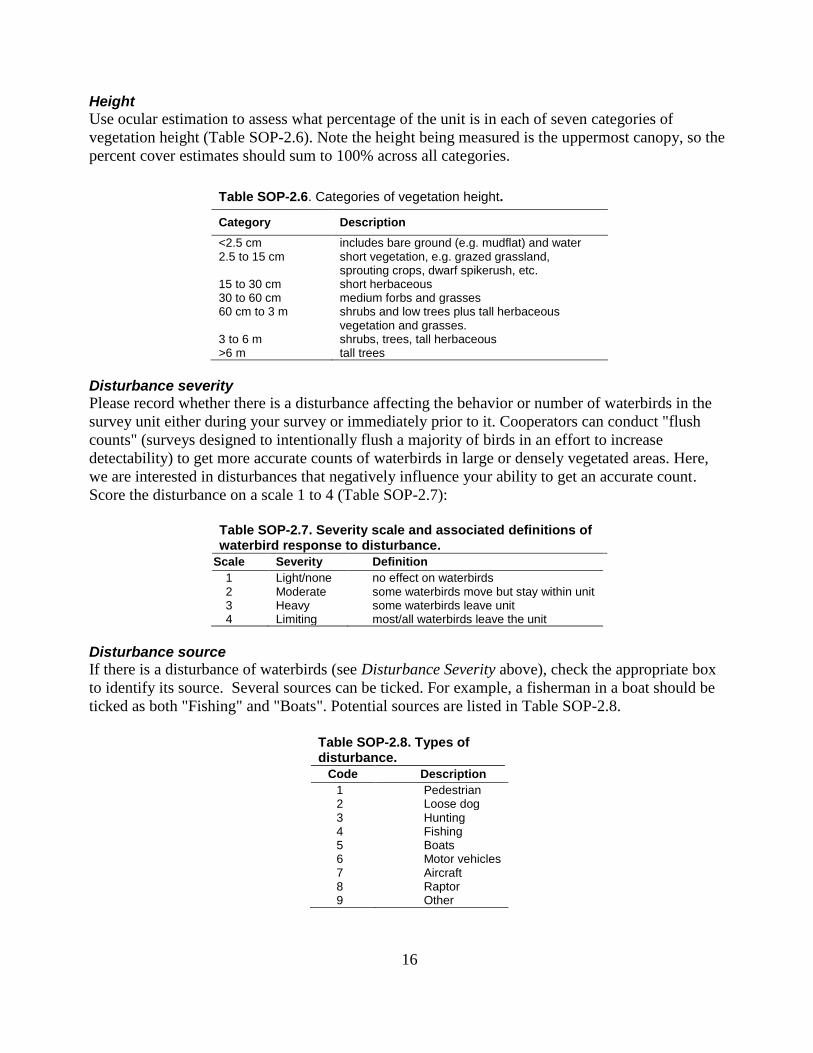
Height

Use ocular estimation to assess what percentage of the unit is in each of seven categories of

vegetation height (Table SOP-2.6). Note the height being measured is the uppermost canopy, so the

percent cover estimates should sum to 100% across all categories.

Table SOP-2.6. Categories of vegetation height.

Category Description

<2.5 cm includes bare ground (e.g. mudflat) and water 2.5 to 15 cm short vegetation, e.g. grazed grassland,

sprouting crops, dwarf spikerush, etc. 15 to 30 cm short herbaceous 30 to 60 cm medium forbs and grasses 60 cm to 3 m shrubs and low trees plus tall herbaceous

vegetation and grasses. 3 to 6 m shrubs, trees, tall herbaceous >6 m tall trees

Disturbance severity

Please record whether there is a disturbance affecting the behavior or number of waterbirds in the

survey unit either during your survey or immediately prior to it. Cooperators can conduct "flush

counts" (surveys designed to intentionally flush a majority of birds in an effort to increase

detectability) to get more accurate counts of waterbirds in large or densely vegetated areas. Here,

we are interested in disturbances that negatively influence your ability to get an accurate count.

Score the disturbance on a scale 1 to 4 (Table SOP-2.7):

Table SOP-2.7. Severity scale and associated definitions of waterbird response to disturbance.

Scale Severity Definition

1 Light/none no effect on waterbirds 2 Moderate some waterbirds move but stay within unit 3 Heavy some waterbirds leave unit 4 Limiting most/all waterbirds leave the unit

Disturbance source

If there is a disturbance of waterbirds (see Disturbance Severity above), check the appropriate box

to identify its source. Several sources can be ticked. For example, a fisherman in a boat should be

ticked as both "Fishing" and "Boats". Potential sources are listed in Table SOP-2.8.

Table SOP-2.8. Types of disturbance.

Code Description

1 Pedestrian 2 Loose dog 3 Hunting 4 Fishing 5 Boats 6 Motor vehicles 7 Aircraft 8 Raptor 9 Other

17

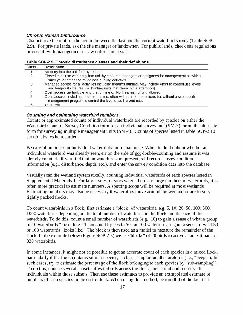
Chronic Human Disturbance

Characterize the unit for the period between the last and the current waterbird survey (Table SOP-

2.9). For private lands, ask the site manager or landowner. For public lands, check site regulations

or consult with management or law enforcement staff.

Table SOP-2.9. Chronic disturbance classes and their definitions.

Class Description

1 No entry into the unit for any reason. 2 Closed to all use with entry into unit by resource managers or designees for management activities,

surveys, or other controlled non-hunting activities. 3 Managed access for all activities including firearms hunting. May include effort to control use levels

and temporal closures (i.e. hunting units that close in the afternoon). 4 Open access via trail, viewing platforms etc. No firearms hunting allowed. 5 Open access, including firearms hunting, often with routine restrictions but without a site specific

management program to control the level of authorized use. 6 Unknown

Counting and estimating waterbird numbers

Counts or approximated counts of individual waterbirds are recorded by species on either the

Waterbird Count or Survey Condition form for an individual survey unit (SM-3), or on the alternate

form for surveying multiple management units (SM-4). Counts of species listed in table SOP-2.10

should always be recorded.

Be careful not to count individual waterbirds more than once. When in doubt about whether an

individual waterbird was already seen, err on the side of not double-counting and assume it was

already counted. If you find that no waterbirds are present, still record survey condition

information (e.g., disturbance, depth, etc.), and enter the survey condition data into the database.

Visually scan the wetland systematically, counting individual waterbirds of each species listed in

Supplemental Materials 1. For larger sites, or sites where there are large numbers of waterbirds, it is

often more practical to estimate numbers. A spotting scope will be required at most wetlands

Estimating numbers may also be necessary if waterbirds move around the wetland or are in very

tightly packed flocks.

To count waterbirds in a flock, first estimate a ‘block’ of waterbirds, e.g. 5, 10, 20, 50, 100, 500,

1000 waterbirds depending on the total number of waterbirds in the flock and the size of the

waterbirds. To do this, count a small number of waterbirds (e.g., 10) to gain a sense of what a group

of 10 waterbirds “looks like.” Then count by 10s to 50s or 100 waterbirds to gain a sense of what 50

or 100 waterbirds “looks like.” The block is then used as a model to measure the remainder of the

flock. In the example below (Figure SOP-2.3) we use 'blocks" of 20 birds to arrive at an estimate of

320 waterbirds.

In some instances, it might not be possible to get an accurate count of each species in a mixed flock,

particularly if the flock contains similar species, such as scaup or small shorebirds (i.e., “peeps”). In

such cases, try to estimate the percentage of the flock belonging to each species by “sub-sampling”.

To do this, choose several subsets of waterbirds across the flock, then count and identify all

individuals within those subsets. Then use these estimates to provide an extrapolated estimate of

numbers of each species in the entire flock. When using this method, be mindful of the fact that

18

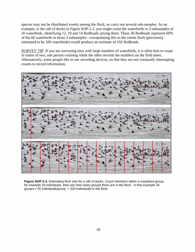
species may not be distributed evenly among the flock, so carry out several sub-samples. As an

example, in the raft of ducks in Figure SOP-2.3, you might count the waterbirds in 3 subsamples of

20 waterbirds, identifying 12, 10 and 14 Redheads among them. These 36 Redheads represent 60%

of the 60 waterbirds in those 3 subsamples - extrapolating this to the whole flock (previously

estimated to be 320 waterbirds) would produce an estimate of 192 Redheads.

SURVEY TIP: If you are surveying sites with large numbers of waterbirds, it is often best to count

in teams of two, one person counting while the other records the numbers on the field sheet.

Alternatively, some people like to use recording devices, so that they are not constantly interrupting

counts to record information.

Figure SOP-2.3. Estimating flock size for a raft of ducks. Count members within a visualized group, for example 20 individuals, then see how many groups there are in the flock. In this example 16 groups x 20 individuals/group = 320 individuals in the flock.

19

Training—First-time IWMM cooperators should view the IWMM overview entitled IWMM

Introduction located at http://iwmmprogram.ning.com/page/presentations.

Inexperienced waterbird counters are advised to practice their counting and estimation techniques

before participating in IWMM. This can be done in the field or at a desktop computer using

Wildlife Counts software: http://wildlifecounts.com/index.html.

Young waterbirds/broods—Do not include dependent young waterbirds in counts. For geese, swans

and ducks, assume juveniles are independent when they can fly. Any juveniles that did not hatch in

the immediate vicinity should be included in counts (e.g. juvenile swans migrating in family

groups).

Special survey techniques

Aerial Surveys—Although we do not require aerial waterbird surveys in the IWMM approach, we

would very much like to include aerial survey data if they are being completed for sites

participating in the program. If you conduct aerial surveys, collect the same data as a standard

ground-based whole-area count, using the same waterbird survey form.

If aerial surveys are employed, the cooperators should note this in the IWMM database. In the bird

survey database form select "Aerial Surveys" in the "Survey Type" dropdown box.

Flush Counts—Cooperators can conduct "flush counts" to get more accurate counts of waterbirds in

large or densely vegetated areas. Flush counts are not required by IWMM, but if this method is

employed, the cooperators should note this in the IWMM database. In the bird survey database form

select "Flush Counts" in the "Survey Type" dropdown box.

References

Cowardin LM, Carter V, Golet FC, LaRoe ET. 1979. Classification of wetlands and deepwater

habitats of the United States. U.S. Fish and Wildlife Service, Washington, D.C.

Fredrickson LH, Reid FA. 1991. 13.1.1 Nutritional values of waterfowl foods, Waterfowl

Management Handbook. U.S. Fish and Wildlife Service, Washington, D.C.

Ma Z, Cai Y, Li B, Chen J. 2010. Managing wetland habitats for waterbirds: an international

perspective. Wetlands 30:15–27.

Suir GM, Evers DE, Steyer GD, Sasser CE. 2013. Development of a reproducible method for

determining the quantity of water and its configuration in a marsh landscape. Journal of Coastal

Research, Special Issue 63:110–117.

20

SOP 3: Measuring Salinity

If measuring salinity with a hydrometer, you will also need a large, clear jar and a thermometer.

The protocol for measuring salinity with a hydrometer (EPA 2006):

1. Put the water sample in a hydrometer jar or a large, clear jar.

2. Gently lower the hydrometer into the jar along with a thermometer. Make sure the

hydrometer and thermometer are not touching and that the top of the hydrometer stem

(which is not in the water) is free of water drops.

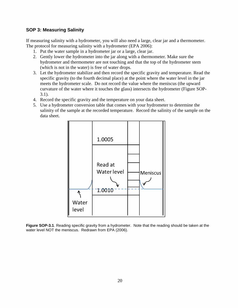
3. Let the hydrometer stabilize and then record the specific gravity and temperature. Read the

specific gravity (to the fourth decimal place) at the point where the water level in the jar

meets the hydrometer scale. Do not record the value where the meniscus (the upward

curvature of the water where it touches the glass) intersects the hydrometer (Figure SOP-

3.1).

4. Record the specific gravity and the temperature on your data sheet.

5. Use a hydrometer conversion table that comes with your hydrometer to determine the

salinity of the sample at the recorded temperature. Record the salinity of the sample on the

data sheet.

Figure SOP-3.1. Reading specific gravity from a hydrometer. Note that the reading should be taken at the water level NOT the meniscus. Redrawn from EPA (2006).

21

If measuring salinity with a refractometer, you will also need a dropper and a container of distilled

water. The protocol for measuring salinity with a refractometer (EPA 2006):

1. Lift the lid that protects the refractometer’s specially angled lens.

2. Place a few drops of your sample liquid on the angled lens and close the lid.

3. Peer through the eyepiece. Results appear along a scale within the eyepiece.

4. Record the measurement on your data sheet.

Rinse the lens with a few drops of distilled water, and pat dry, being very careful to not scratch the

lens’ surface.

References

[EPA] Environmental Protection Agency. 2006. Chapter 14: Salinity Pages 1–8 in Ohrel RL J.,

Register KM, editors. Volunteer estuary monitoring manual, a methods manual. 2nd edition.

Washington, D.C.: EPA-842-B-06-003. Available:

http://water.epa.gov/type/oceb/nep/monitor_index.cfm (January 2015).

22

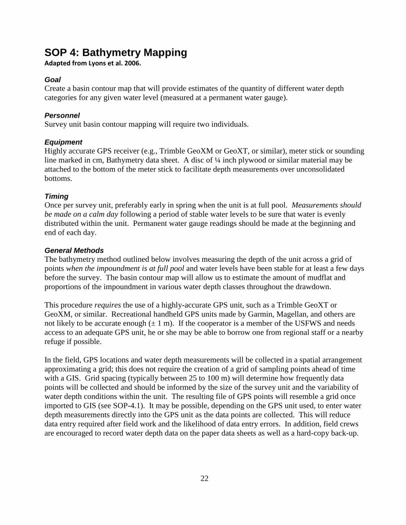
SOP 4: Bathymetry Mapping Adapted from Lyons et al. 2006.

Goal

Create a basin contour map that will provide estimates of the quantity of different water depth

categories for any given water level (measured at a permanent water gauge).

Personnel

Survey unit basin contour mapping will require two individuals.

Equipment

Highly accurate GPS receiver (e.g., Trimble GeoXM or GeoXT, or similar), meter stick or sounding

line marked in cm, Bathymetry data sheet. A disc of ¼ inch plywood or similar material may be

attached to the bottom of the meter stick to facilitate depth measurements over unconsolidated

bottoms.

Timing

Once per survey unit, preferably early in spring when the unit is at full pool. Measurements should

be made on a calm day following a period of stable water levels to be sure that water is evenly

distributed within the unit. Permanent water gauge readings should be made at the beginning and

end of each day.

General Methods

The bathymetry method outlined below involves measuring the depth of the unit across a grid of

points when the impoundment is at full pool and water levels have been stable for at least a few days

before the survey. The basin contour map will allow us to estimate the amount of mudflat and

proportions of the impoundment in various water depth classes throughout the drawdown.

This procedure requires the use of a highly-accurate GPS unit, such as a Trimble GeoXT or

GeoXM, or similar. Recreational handheld GPS units made by Garmin, Magellan, and others are

not likely to be accurate enough (± 1 m). If the cooperator is a member of the USFWS and needs

access to an adequate GPS unit, he or she may be able to borrow one from regional staff or a nearby

refuge if possible.

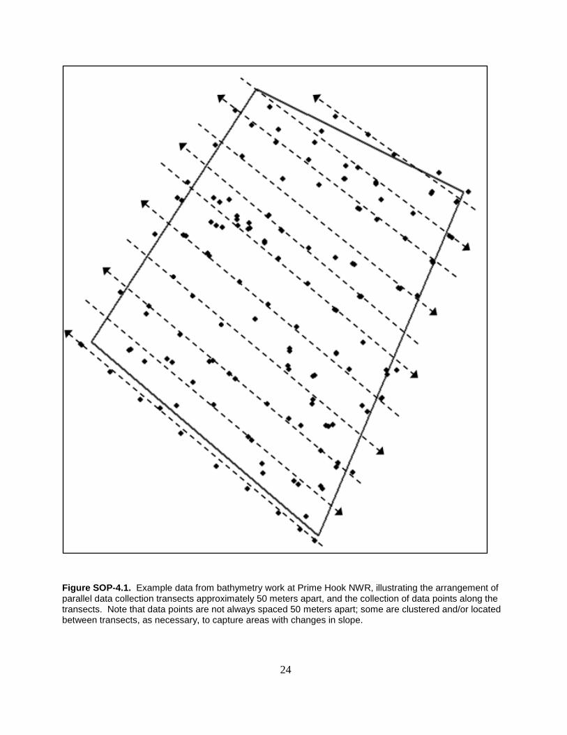
In the field, GPS locations and water depth measurements will be collected in a spatial arrangement

approximating a grid; this does not require the creation of a grid of sampling points ahead of time

with a GIS. Grid spacing (typically between 25 to 100 m) will determine how frequently data

points will be collected and should be informed by the size of the survey unit and the variability of

water depth conditions within the unit. The resulting file of GPS points will resemble a grid once

imported to GIS (see SOP-4.1). It may be possible, depending on the GPS unit used, to enter water

depth measurements directly into the GPS unit as the data points are collected. This will reduce

data entry required after field work and the likelihood of data entry errors. In addition, field crews

are encouraged to record water depth data on the paper data sheets as well as a hard-copy back-up.

23

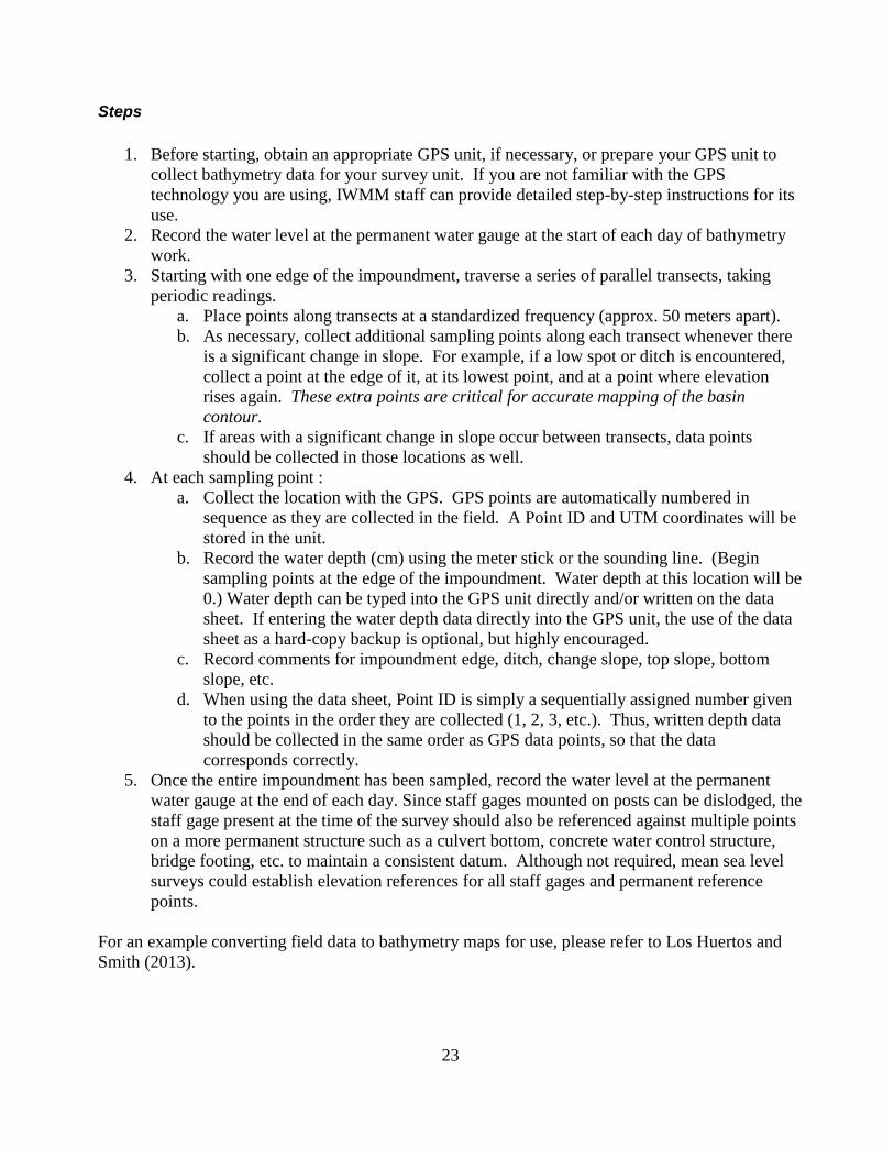
Steps

1. Before starting, obtain an appropriate GPS unit, if necessary, or prepare your GPS unit to

collect bathymetry data for your survey unit. If you are not familiar with the GPS

technology you are using, IWMM staff can provide detailed step-by-step instructions for its

use.

2. Record the water level at the permanent water gauge at the start of each day of bathymetry

work.

3. Starting with one edge of the impoundment, traverse a series of parallel transects, taking

periodic readings.

a. Place points along transects at a standardized frequency (approx. 50 meters apart).

b. As necessary, collect additional sampling points along each transect whenever there

is a significant change in slope. For example, if a low spot or ditch is encountered,

collect a point at the edge of it, at its lowest point, and at a point where elevation

rises again. These extra points are critical for accurate mapping of the basin

contour.

c. If areas with a significant change in slope occur between transects, data points

should be collected in those locations as well.

4. At each sampling point :

a. Collect the location with the GPS. GPS points are automatically numbered in

sequence as they are collected in the field. A Point ID and UTM coordinates will be

stored in the unit.

b. Record the water depth (cm) using the meter stick or the sounding line. (Begin

sampling points at the edge of the impoundment. Water depth at this location will be

0.) Water depth can be typed into the GPS unit directly and/or written on the data

sheet. If entering the water depth data directly into the GPS unit, the use of the data

sheet as a hard-copy backup is optional, but highly encouraged.

c. Record comments for impoundment edge, ditch, change slope, top slope, bottom

slope, etc.

d. When using the data sheet, Point ID is simply a sequentially assigned number given

to the points in the order they are collected (1, 2, 3, etc.). Thus, written depth data

should be collected in the same order as GPS data points, so that the data

corresponds correctly.

5. Once the entire impoundment has been sampled, record the water level at the permanent

water gauge at the end of each day. Since staff gages mounted on posts can be dislodged, the

staff gage present at the time of the survey should also be referenced against multiple points

on a more permanent structure such as a culvert bottom, concrete water control structure,

bridge footing, etc. to maintain a consistent datum. Although not required, mean sea level

surveys could establish elevation references for all staff gages and permanent reference

points.

For an example converting field data to bathymetry maps for use, please refer to Los Huertos and

Smith (2013).

24

Figure SOP-4.1. Example data from bathymetry work at Prime Hook NWR, illustrating the arrangement of parallel data collection transects approximately 50 meters apart, and the collection of data points along the transects. Note that data points are not always spaced 50 meters apart; some are clustered and/or located between transects, as necessary, to capture areas with changes in slope.

25

References

Lyons JE, Runge, MC, Kendall WL, Laskowski H, Lor S, Talbott S. 2006. Timing of impoundment

drawdowns and impact on waterbird, invertebrate, and vegetation communities within managed

wetlands:.Study Manual Final Version Field Season 2006. USGS-Refuge Cooperative Research

Program. Laurel, Maryland.

Los Huertos M, Smith D. 2013. Wetland Bathymetry and Mapping. Pages 49–86 in Anderson JT,

Davis CA, editors. Wetland Techniques: Foundations. Volume 1. Secaucus, New Jersey:

Springer.

26

SOP 5: Vegetation Survey

Follow these instructions for preparing and conducting vegetation surveys and assessing site

conditions of each unit. Associated data collection sheet can be found in Supplemental Materials 7.

Equipment

Map of the site and unit boundaries

Annual Vegetation Survey Form (See Supplemental Materials 4)

Seed Head Photographic Guide (See Supplemental Materials 5)

Survey Schedule

Vegetation surveys are to be completed once annually, typically late in the growing season when

dominant plant species have started to senesce. To improve the accuracy of the seed head index,

surveys should also be completed prior to the shattering of influential moist-soil species.

Plant Community Composition

Plant community composition will be assessed by measuring the cover of individual, emergent plant

species in areas of emergent vegetation within the survey unit. Only emergent vegetation from

the current growing season should be included in plant community composition assessments.

Two major steps are involved in the assessment of plant community composition: (1) assessment of

percent emergent cover within the survey unit and (2) species inventory and species-specific

percent cover assessments within areas of emergent vegetation.

Cooperators should determine the location of all emergent vegetation patches within a survey unit.

This could be done through a visual assessment around the perimeter of the survey unit. Preferably,

patches would be identified via a combination of aerial photograph (e.g., Google Earth imagery)

and field-based visual inspections. Once the cooperator is confident they have identified all

emergent vegetation patches, they should estimate and record the percent of the survey unit covered

by emergent vegetation. Percent cover is defined as the percentage of the survey unit covered by

vertical projections from the outermost perimeter of plants’ foliage (Anderson 1986) (Figure SOP-

5.1). Again, for this metric, percent cover assessments should exclusively consider vegetation from

the current season’s growth.

27

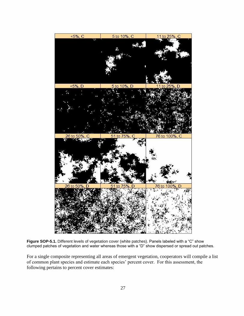
Figure SOP-5.1. Different levels of vegetation cover (white patches). Panels labeled with a “C” show clumped patches of vegetation and water whereas those with a “D” show dispersed or spread out patches.

For a single composite representing all areas of emergent vegetation, cooperators will compile a list

of common plant species and estimate each species’ percent cover. For this assessment, the

following pertains to percent cover estimates:

28

For individual plant species, cover is defined as above except that it is estimated as a

percentage of emergent vegetation area not as a percentage of total survey unit area. As an

example, consider a survey unit that contains only cattail as an emergent plant species.

Cattail may cover 50% of the total survey unit area, but as an individual plant species, it

covers 100% of the emergent vegetation area within a survey unit; report 100% as the

estimate.

Cover should be estimated only for common species, species covering >5% of the emergent

vegetation area.

Total cover across species can exceed 100% due to the stratification of plant species with

varying heights and growth forms.

Cooperators have two options for creating a list of the common plants and estimating their percent

covers:

1. Entry, Ocular Assessments (Preferred)

Preferably, cooperators will be able to physically enter the unit to identify emergent plant species

and to assess their covers. Physical entry will especially help cooperators identify and account for

plant species occupying lower strata that may be over-topped by taller growth forms.

2. Non-entry, Ocular Assessments (Non-preferred)

While not the preferred option, cooperators can identify emergent species and assess their covers

entirely from vantage points around the perimeter of the survey unit. Vantage points should offer

cooperators a comprehensive view of the emergent vegetation within the unit. This may be the only

viable assessment option when a cooperator does not have permission to enter a unit.

Seed Head Assessments

For important waterfowl food species identified in the Plant Community Composition assessment

(see above), choose a category for seed-head size and density for each species (Naylor et al. 2005).

Using ocular estimation, qualitatively assess seed head size for a given species as average, smaller,

or larger than the average size for the species. For example, Polygonum pensylvanicum would be

compared to average size of seed heads for this species. Use the “Not Assessed” category for

species that have deteriorated seed heads at the time of assessment or difficult to assess seed heads.

We provide a photographic guide to assist you in making seed head size assessments (see

Supplemental Materials 6). The guide includes many common waterfowl food sources but may

exclude some regionally important species. If you encounter a species that is energetically

important and not listed in the photographic guide, please email iwmmprogram@gmail.com to

suggest the species as an addition to the guide.

For each common plant species, visually assess seed head density based on two considerations:

The density of stems for a species.

The proportion of a species’ stems with seed heads

29

Through ocular assessments, seed head density is assigned to ordinal categories including low,

moderate, or high. Low seed head density is characterized by large areas of bare ground and a low

proportion of seed heads to plant stems. High stem density is assigned to areas with little bare

ground and a high proportion of seed heads to stems. Moderate stem densities fall between these

two extremes. Percent near tall edge

A “tall edge” is defined as an edge of the survey unit bordered by trees >6 m tall. There are two

alternatives for assessing the percent of a survey unit near a tall edge.

1. Aerial Photograph Assessment (Preferred)

The preferred option is to use available imagery in Google Earth or other remote sensing images to

assess what percentage of the survey unit is within 50 m of a tall edge.

2. Ocular Assessment (Non-preferred)

While not the preferred option, observers may visually assess the percentage of the unit within 50 m

of a tall edge. This option should be employed only if available aerial imagery for a survey unit no

longer reflects conditions on the ground, i.e., the photo is too old to use for the assessment.

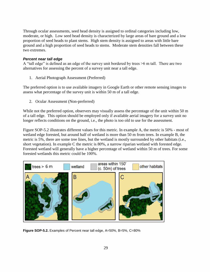
Figure SOP-5.2 illustrates different values for this metric. In example A, the metric is 50% - most of

wetland edge forested, but around half of wetland is more than 50 m from trees. In example B, the

metric is 5%, there are some tree lines, but the wetland is mostly surrounded by other habitats (i.e.,

short vegetation). In example C the metric is 80%, a narrow riparian wetland with forested edge.

Forested wetland will generally have a higher percentage of wetland within 50 m of trees. For some

forested wetlands this metric could be 100%.

Figure SOP-5.2. Examples of Percent near tall edge, A=50%, B=5%, C=80%

30

References

Anderson EW. 1986. A guide for estimating cover. Rangelands 8:236–238.

Naylor LW, Eadie JM, Smith WD, Eichholz M, Gray MJ. 2005. A simple method to predict seed

yield in moist-soil habitats. Wildlife Society Bulletin 33:1335–1341.

SOP 6: Recording Management Actions

Follow these instructions for recording and tracking management actions for each unit surveyed.

Associated management record sheet can be found in Supplemental Materials 7. Resources

Map of the site and unit boundaries

Wetland management activities record (Supplemental Materials 7) for recording

implemented actions.

In addition to monitoring waterbird use and habitat response, routine habitat management activities

need to be tracked for each management unit. To develop effective and informed strategies in an

adaptive management approach, a reasonable range of management activities must be considered

(Williams 2011). The details of timing, extent, and frequency will be recorded by cooperators via a

wetland management record (Supplemental Materials 7) to document individual actions (as listed in

Table SOP-6.1) as planned and implemented prescriptions. Infrequent management activities

involving major modifications or infrastructure development are excluded.

1. Create wetland management activities record (Supplemental Materials 7) for each unit and

fill in all planned actions. Use annual habitat management plans or other annual goals &

objectives to match planned activities for a unit to an action code in Table SOP-6.1. Broad

classes are provided to narrow the search for matching actions. Start the annual tracking

period at the beginning of the growing season that precedes the subsequent nonbreeding

period.

2. Update the record through the season as actions are implemented. Create a new entry for

repeat applications when the interval between applications exceeds the time required for a

single application. Record the geographic extent (footprint as the proportion of a

management unit) for each log entry. Total percent manipulated may exceed 100% since

applications may overlap.

3. Cooperators should enter information from the management action record into IWMM’s

centralized, online database on a routine basis with a complete entry concurrent with the last

waterbird survey for a survey period.

The following action groups are provided to guide the selection of individual actions:

31

Agriculture—Includes all activities related to the production of a harvested crop or a crop left

standing. Cultivation or other actions commonly used in agriculture are excluded if a crop was not

produced. Sowed stands of millet cultivars should be included here but not volunteer stands.

Chemical—Use of herbicides or fertilizers to manage vegetation not related to crop production.

Fire-Prescribed—Controlled burns completed within a range of prescriptions described in an

approved burn plan.

Mechanical—Managing soil, herbaceous vegetation, or light woody vegetation <4.5 inches diameter

at breast height (dbh) with mechanized equipment. Action includes common agricultural tillage

practices not related to the production of a crop in the current year.

Mechanical-woody—Removal or other manipulation of tree size (> 4.5 inches dbh) woody

vegetation.

Prescribed grazing—Controlled grazing completed within a range of prescriptions described in an

approved grazing plan.

Restoration herbaceous—Introducing seed of desired non-crop herbaceous vegetation.

Restoration woody—Actions relating to the direct planting or promotion of woody vegetation

through natural succession.

Water level management—Actions applied to manipulate water levels through adjusting water

control structures, pumping, or facilitating water movement.

A strategy list from the Refuge Lands Geographic Information System (RLGIS, USFWS 2010)

served as foundation for a compiled list of actions (Table SOP-6.1). The RLGIS Actions were

modified and fitted with costs from Natural Resources Conservation Service (NRCS) cost-share

practices (NRCS 2012, NRCS 2014 a, b). Pumping logs, pump specifications, power source fuel

use, and an irrigation study served as a basis for the fuel-use based pumping cost estimates (SRS

Crisafulli Inc. 2014, University of NE 2011, Henggeler 2012). Crop input costs are based on

production agriculture cost estimates (Dhuyvetter et al., Dobbins et al. 2012, Duffy 2014, Greer et

al. 2012, USDA 2012). Estimates for prescribed goat grazing in wetlands and mechanical marsh

shredders are derived from Greenfield et al. (2006). Costs for chemical control of woody invasive

plants based on Rathfon and Ruble (2006) and NRCS (2012).

All costs estimates are very general and applied to actions with highly variable costs. The estimates

are not recommended for use in budgeting purposes, cost benefit analysis, or other purposes

requiring increased accuracy. When available, site-specific cost estimates can be used in lieu of the

estimates provided to support of local-scale decision support tools or other uses.

32

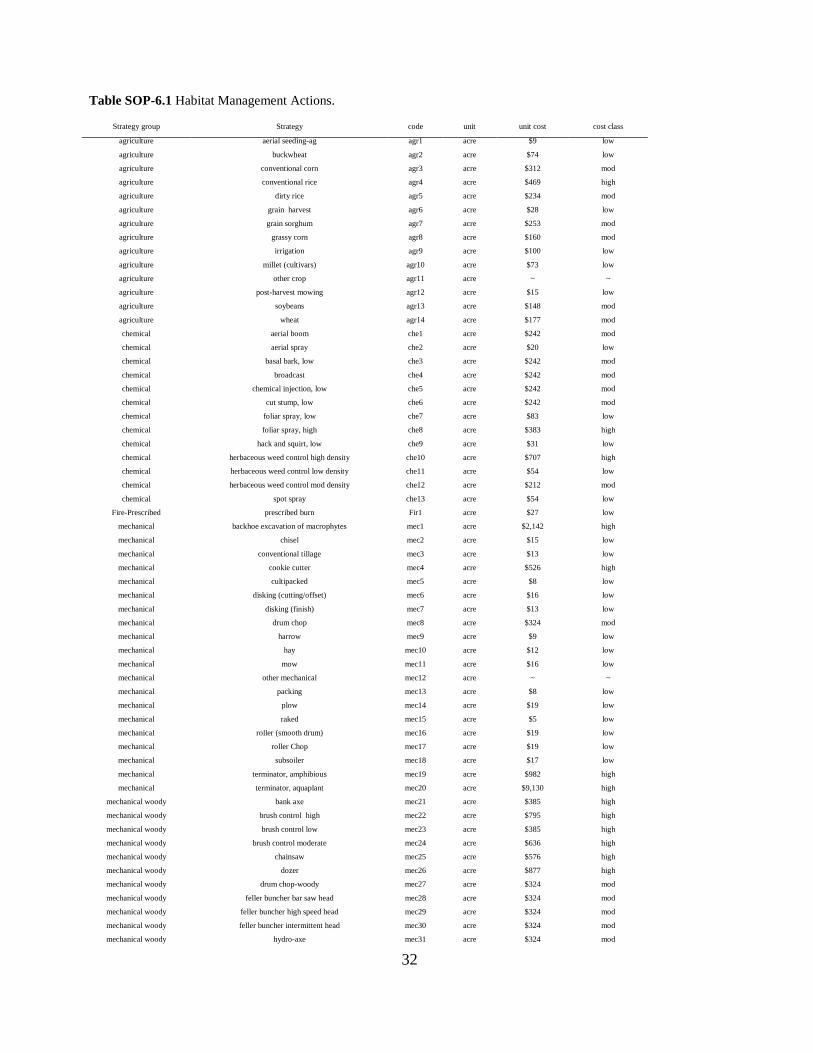
Table SOP-6.1 Habitat Management Actions.

Strategy group Strategy code unit unit cost cost class

agriculture aerial seeding-ag agr1 acre $9 low

agriculture buckwheat agr2 acre $74 low

agriculture conventional corn agr3 acre $312 mod

agriculture conventional rice agr4 acre $469 high

agriculture dirty rice agr5 acre $234 mod

agriculture grain harvest agr6 acre $28 low

agriculture grain sorghum agr7 acre $253 mod

agriculture grassy corn agr8 acre $160 mod

agriculture irrigation agr9 acre $100 low

agriculture millet (cultivars) agr10 acre $73 low

agriculture other crop agr11 acre ~ ~

agriculture post-harvest mowing agr12 acre $15 low

agriculture soybeans agr13 acre $148 mod

agriculture wheat agr14 acre $177 mod

chemical aerial boom che1 acre $242 mod

chemical aerial spray che2 acre $20 low

chemical basal bark, low che3 acre $242 mod

chemical broadcast che4 acre $242 mod

chemical chemical injection, low che5 acre $242 mod

chemical cut stump, low che6 acre $242 mod

chemical foliar spray, low che7 acre $83 low

chemical foliar spray, high che8 acre $383 high

chemical hack and squirt, low che9 acre $31 low

chemical herbaceous weed control high density che10 acre $707 high

chemical herbaceous weed control low density che11 acre $54 low

chemical herbaceous weed control mod density che12 acre $212 mod

chemical spot spray che13 acre $54 low

Fire-Prescribed prescribed burn Fir1 acre $27 low

mechanical backhoe excavation of macrophytes mec1 acre $2,142 high

mechanical chisel mec2 acre $15 low

mechanical conventional tillage mec3 acre $13 low

mechanical cookie cutter mec4 acre $526 high

mechanical cultipacked mec5 acre $8 low

mechanical disking (cutting/offset) mec6 acre $16 low

mechanical disking (finish) mec7 acre $13 low

mechanical drum chop mec8 acre $324 mod

mechanical harrow mec9 acre $9 low

mechanical hay mec10 acre $12 low

mechanical mow mec11 acre $16 low

mechanical other mechanical mec12 acre ~ ~

mechanical packing mec13 acre $8 low

mechanical plow mec14 acre $19 low

mechanical raked mec15 acre $5 low

mechanical roller (smooth drum) mec16 acre $19 low

mechanical roller Chop mec17 acre $19 low

mechanical subsoiler mec18 acre $17 low

mechanical terminator, amphibious mec19 acre $982 high

mechanical terminator, aquaplant mec20 acre $9,130 high

mechanical woody bank axe mec21 acre $385 high

mechanical woody brush control high mec22 acre $795 high

mechanical woody brush control low mec23 acre $385 high

mechanical woody brush control moderate mec24 acre $636 high

mechanical woody chainsaw mec25 acre $576 high

mechanical woody dozer mec26 acre $877 high

mechanical woody drum chop-woody mec27 acre $324 mod

mechanical woody feller buncher bar saw head mec28 acre $324 mod

mechanical woody feller buncher high speed head mec29 acre $324 mod

mechanical woody feller buncher intermittent head mec30 acre $324 mod

mechanical woody hydro-axe mec31 acre $324 mod

33

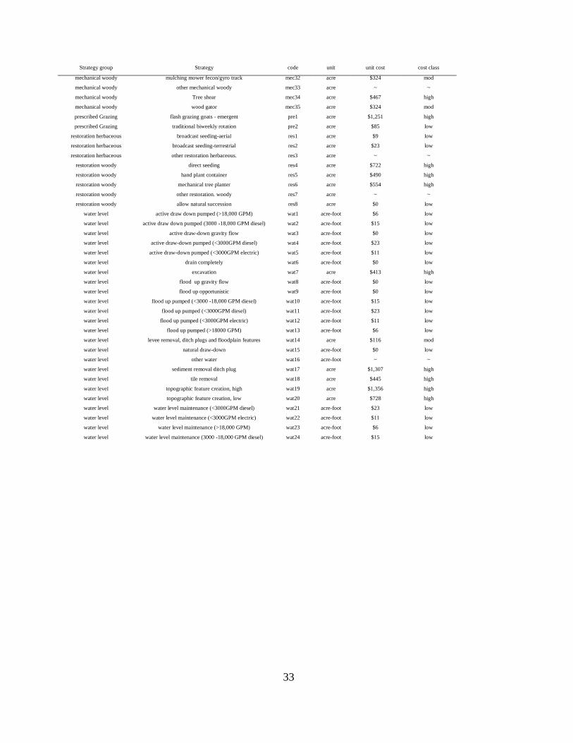
Strategy group Strategy code unit unit cost cost class

mechanical woody mulching mower fecon/gyro track mec32 acre $324 mod

mechanical woody other mechanical woody mec33 acre ~ ~

mechanical woody Tree shear mec34 acre $467 high

mechanical woody wood gator mec35 acre $324 mod

prescribed Grazing flash grazing goats - emergent pre1 acre $1,251 high

prescribed Grazing traditional biweekly rotation pre2 acre $85 low

restoration herbaceous broadcast seeding-aerial res1 acre $9 low

restoration herbaceous broadcast seeding-terrestrial res2 acre $23 low

restoration herbaceous other restoration herbaceous. res3 acre ~ ~

restoration woody direct seeding res4 acre $722 high

restoration woody hand plant container res5 acre $490 high

restoration woody mechanical tree planter res6 acre $554 high

restoration woody other restoration. woody res7 acre ~ ~

restoration woody allow natural succession res8 acre $0 low

water level active draw down pumped (>18,000 GPM) wat1 acre-foot $6 low

water level active draw down pumped (3000 -18,000 GPM diesel) wat2 acre-foot $15 low

water level active draw-down gravity flow wat3 acre-foot $0 low

water level active draw-down pumped (<3000GPM diesel) wat4 acre-foot $23 low

water level active draw-down pumped (<3000GPM electric) wat5 acre-foot $11 low

water level drain completely wat6 acre-foot $0 low

water level excavation wat7 acre $413 high

water level flood up gravity flow wat8 acre-foot $0 low

water level flood up opportunistic wat9 acre-foot $0 low

water level flood up pumped (<3000 -18,000 GPM diesel) wat10 acre-foot $15 low

water level flood up pumped (<3000GPM diesel) wat11 acre-foot $23 low

water level flood up pumped (<3000GPM electric) wat12 acre-foot $11 low

water level flood up pumped (>18000 GPM) wat13 acre-foot $6 low

water level levee removal, ditch plugs and floodplain features wat14 acre $116 mod

water level natural draw-down wat15 acre-foot $0 low

water level other water wat16 acre-foot ~ ~

water level sediment removal ditch plug wat17 acre $1,307 high

water level tile removal wat18 acre $445 high

water level topographic feature creation, high wat19 acre $1,356 high

water level topographic feature creation, low wat20 acre $728 high

water level water level maintenance (<3000GPM diesel) wat21 acre-foot $23 low

water level water level maintenance (<3000GPM electric) wat22 acre-foot $11 low

water level water level maintenance (>18,000 GPM) wat23 acre-foot $6 low

water level water level maintenance (3000 -18,000 GPM diesel) wat24 acre-foot $15 low

34

References

Dhuyvetter KC, O’Brien DM, Douglas S. 2014. Grain Sorghum Cost-Return Budget in Southeast

Kansas, Kansas State University. Manhattan. Farm Management Guide MF995.

Dobbins CL, Langemeier MR, Miller WA, Nielsen B, Vyn TJ, Casteel S, Johnson BB, Wise K.

2012. 2013 Purdue Crop Cost & Return Guide. Cooperative Extension Service Purdue

University. West Lafayette, Indiana.

Duffy M. 2014. Estimated Costs of Crop Production in Iowa: 2014 File A1-20. Cooperative

Extension Service Iowa State University of Science and Technology, Ames, Iowa.

Greenfield BK, Blankinship M, McNabb TJ. 2006. Control Costs, Operation, and Permitting Issues

for Non-chemical Plant Control: Case Studies in the San Francisco Bay-Delta Region,

California. Journal of Aquatic Plant Management 44:40–49.

Greer CA, Mutters RG, Espino LA, Buttner P, Klonsky KM, De Moura RL, Tumber KP. 2012.

Sample Costs to Produce Rice. Department of Agricultural and Resource Economics,

University of California, Davis.

Henggeler JC. 2012. Irrigation Systems, Wells, and Pumps of the Mississippi River Alluvium

Aquifer of Southeast Missouri. T.E. “Jake” Fisher Delta Center. Commercial Agriculture

Program, University of Missouri Extension. Columbia.

Natural Resources Conservation Service. 2012. FY2013 Practice Payment Schedule for

EQIP/WHIP. Available:

http://www.nrcs.usda.gov/Internet/FSE_DOCUMENTS/nrcs141p2_035967.pdf (April 2014).

Natural Resources Conservation Service. 2014a. Working Lands for Wildlife 2014 Payment

Schedule. Available:

http://www.nrcs.usda.gov/wps/PA_NRCSConsumption/download?cid=stelprdb1247312&ext=p

df (April 2014).

Natural Resources Conservation Service. 2014b. FY2014 Payment Scenario Descriptions for

Illinois. Available:

http://www.nrcs.usda.gov/wps/PA_NRCSConsumption/download?cid=stelprdb1243994&ext=x

lsx (April 2014).

Rathfon, R and Ruble K. 2006. Herbicide Treatments for Controlling Invasive Bush Honeysuckle in

a Mature Hardwood Forest in West-central Indiana. Pages 187-197 in Buckley DS, Clatterbuck

WK, editors. Proceedings 15th Central Hardwood Forest Conference. Asheville, North

Carolina, U.S. Department of Agriculture Forest Service, Southern Research Station.

SRS Crisafulli Inc. 2014. Trailer Pumps Product Catalogue. Available:

http://www.crisafullipumps.com/products-services/pumps/trailer/. (April 2014).

35

University of Missouri Extension. 2012. 2012 Custom Rates for Farm Services in Missouri.

Cooperative Extension University of Missouri. Columbia.

University of Nebraska Lincoln. 2011. Nebraska OECD Tractor Test 1987-Summary 760.

Nebraska Tractor Test Laboratory University of Nebraska Lincoln, East Campus. Lincoln.

USDA. 2012. Conservation Systems Fact Sheet No. 040. National Soil Dynamics Laboratory.

Auburn, Alabama.

Williams BK. 2011. Adaptive management of natural resources: framework and issues. Journal of

Environmental Management 92.5:1346–1353.

Williams BK, Szaro RC, Shapiro CD. 2009. Adaptive Management: The U.S. Department of

Interior Technical Guide. Adaptive Management Working Group, U.S. Department of Interior,

Washington, D.C.

36

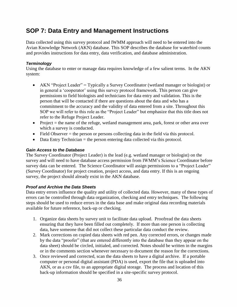
SOP 7: Data Entry and Management Instructions

Data collected using this survey protocol and IWMM approach will need to be entered into the

Avian Knowledge Network (AKN) database. This SOP describes the database for waterbird counts

and provides instructions for data entry, data verification, and database administration.

Terminology

Using the database to enter or manage data requires knowledge of a few salient terms. In the AKN

system:

AKN “Project Leader” = Typically a Survey Coordinator (wetland manager or biologist) or

in general a ‘cooperator’ using this survey protocol framework. This person can give

permissions to field biologists and technicians for data entry and validation. This is the

person that will be contacted if there are questions about the data and who has a

commitment to the accuracy and the validity of data entered from a site. Throughout this

SOP we will refer to this role as the “Project Leader” but emphasize that this title does not

refer to the Refuge Project Leader.

Project = the name of the refuge, wetland management area, park, forest or other area over

which a survey is conducted.

Field Observer = the person or persons collecting data in the field via this protocol.

Data Entry Technician = the person entering data collected via this protocol.

Gain Access to the Database

The Survey Coordinator (Project Leader) is the lead (e.g. wetland manager or biologist) on the

survey and will need to have database access permission from IWMM’s Science Coordinator before

survey data can be entered. The Science Coordinator will assign permissions to a “Project Leader”

(Survey Coordinator) for project creation, project access, and data entry. If this is an ongoing

survey, the project should already exist in the AKN database.

Proof and Archive the Data Sheets

Data entry errors influence the quality and utility of collected data. However, many of these types of

errors can be controlled through data organization, checking and entry techniques. The following

steps should be used to reduce errors in the data base and make original data recording materials

available for future reference, back-up or checking.

1. Organize data sheets by survey unit to facilitate data upload. Proofread the data sheets

ensuring that they have been filled out completely. If more than one person is collecting

data, have someone that did not collect these particular data conduct the review.

2. Mark corrections on copied data sheets with red pen. Any corrected errors, or changes made

by the data “proofer” (that are entered differently into the database than they appear on the

data sheet) should be circled, initialed, and corrected. Notes should be written in the margins

or in the comments section whenever necessary to document the reason for the corrections.

3. Once reviewed and corrected, scan the data sheets to have a digital archive. If a portable

computer or personal digital assistant (PDA) is used, export the file that is uploaded into

AKN, or as a csv file, to an appropriate digital storage. The process and location of this

back-up information should be specified in a site-specific survey protocol.

37

4. After data entry into AKN, archive the scanned data sheets or exported PDA file. If the data

are associated with a survey report, include these data as an Appendix to the report and

archive the report if possible. The original completed data forms or PDA file can also be

stored on site in a safe place, preferably in a designated fireproof safe or cabinet.

Enter the Data

Prepare for data entry:

1. Organize your data and guidance materials to aid data entry process.

2. A data form will help verify that you have all the right data entry fields for your project.

3. A description or knowledge of the methods used for this survey.

4. The name and address of the Survey Coordinator (the person who can be contacted

regarding questions about these data, once entered).

Enter the data into the AKN database:

1. Contact the IWMM Science Coordinator to gain access and log in to the data entry web site

using your email address and password.

2. Enter all waterbird, unit condition, and vegetation data from the datasheet into the database.

The database is intended to accept data uploaded from spreadsheets or stand-alone

databases. Check with IWMM’s Science Coordinator or website to determine formats that

can be accepted for uploading waterbird data.

3. After all data from each data sheet have been entered or uploaded, proof the data in the

database, reviewing the data forms and sorting summaries (from queries) to check for typos,

errors, and blank fields. As each data sheet (or any PDA output) is proofed, date and initial

that the input data were reviewed and checked against the original data records. The data

entry person will also verify the data has been proofed in the database by changing the status

of the data records to the next appropriate level (see the user’s manual for the database).

Verify and Validate

In general, AKN uses a tiered set of levels for indicating the data validation and access (Table SOP-

7.1). Once the person entering data is finished, he or she needs to notify the “Project Leader”

responsible for AKN data management (for the Refuge System, this is typically the survey

coordinator) that data are ready to be proofed in the database. The Project Leader will:

1. Ensure all datasheets have been initialed.

2. Compare the data sheets with the data records in the database and if there are no errors, then

change the status of the records to the next appropriate level (see the user’s manual for the

database).

3. Discuss any questionable data entry or field observer errors with the Data Entry Technician

and/or Field Observer. If there are errors, the Project Leader will open up the records for

editing.

4. After all errors are satisfactorily resolved in the database, the Project Leader will change the

status of the records in the database.

38

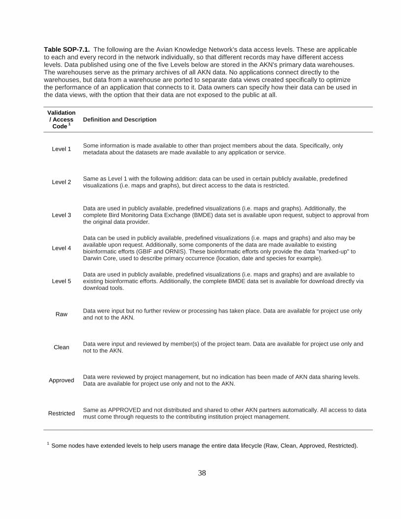
Table SOP-7.1. The following are the Avian Knowledge Network's data access levels. These are applicable to each and every record in the network individually, so that different records may have different access levels. Data published using one of the five Levels below are stored in the AKN's primary data warehouses. The warehouses serve as the primary archives of all AKN data. No applications connect directly to the warehouses, but data from a warehouse are ported to separate data views created specifically to optimize the performance of an application that connects to it. Data owners can specify how their data can be used in the data views, with the option that their data are not exposed to the public at all.

Validation / Access Code

1

Definition and Description

Level 1 Some information is made available to other than project members about the data. Specifically, only metadata about the datasets are made available to any application or service.

Level 2 Same as Level 1 with the following addition: data can be used in certain publicly available, predefined visualizations (i.e. maps and graphs), but direct access to the data is restricted.

Level 3 Data are used in publicly available, predefined visualizations (i.e. maps and graphs). Additionally, the complete Bird Monitoring Data Exchange (BMDE) data set is available upon request, subject to approval from the original data provider.

Level 4

Data can be used in publicly available, predefined visualizations (i.e. maps and graphs) and also may be available upon request. Additionally, some components of the data are made available to existing bioinformatic efforts (GBIF and ORNIS). These bioinformatic efforts only provide the data "marked-up" to Darwin Core, used to describe primary occurrence (location, date and species for example).

Level 5 Data are used in publicly available, predefined visualizations (i.e. maps and graphs) and are available to existing bioinformatic efforts. Additionally, the complete BMDE data set is available for download directly via download tools.

Raw Data were input but no further review or processing has taken place. Data are available for project use only and not to the AKN.

Clean Data were input and reviewed by member(s) of the project team. Data are available for project use only and not to the AKN.

Approved Data were reviewed by project management, but no indication has been made of AKN data sharing levels. Data are available for project use only and not to the AKN.

Restricted Same as APPROVED and not distributed and shared to other AKN partners automatically. All access to data must come through requests to the contributing institution project management.

1 Some nodes have extended levels to help users manage the entire data lifecycle (Raw, Clean, Approved, Restricted).

39

Data Maintenance and Archiving

AKN is responsible for performing periodic backups of all data residing in the database.

Editing of data that has already been “verified” in the database must be made in the AKN database

by the Project Leader via the interface. Contact IWMM’s Science Coordinator for assistance if

numerous edits are needed.