Integrated Supply Chain Network Design: Location ... Supply Chain Network Design: Location,...

Integrated Supply Chain Network Design:

Location, Transportation, Routing and Inventory Decisions

by

Mingjun Xia

A Dissertation Presented in Partial Fulfillment of the Requirements for the Degree

Doctor of Philosophy

Approved April 2013 by the Graduate Supervisory Committee:

Ronald Askin, Chair

Pitu Mirchandani Muhong Zhang Henry Kierstead

ARIZONA STATE UNIVERSITY

May 2013

i

ABSTRACT

In this dissertation, an innovative framework for designing a multi-product integrated

supply chain network is proposed. Multiple products are shipped from production

facilities to retailers through a network of Distribution Centers (DCs). Each retailer has

an independent, random demand for multiple products. The particular problem

considered in this study also involves mixed-product transshipments between DCs with

multiple truck size selection and routing delivery to retailers.

Optimally solving such an integrated problem is in general not easy due to its

combinatorial nature, especially when transshipments and routing are involved. In order

to find out a good solution effectively, a two-phase solution methodology is derived:

Phase I solves an integer programming model which includes all the constraints in the

original model except that the routings are simplified to direct shipments by using

estimated routing cost parameters. Then Phase II model solves the lower level inventory

routing problem for each opened DC and its assigned retailers.

The accuracy of the estimated routing cost and the effectiveness of the two-phase

solution methodology are evaluated, the computational performance is found to be

promising. The problem is able to be heuristically solved within a reasonable time frame

for a broad range of problem sizes (one hour for the instance of 200 retailers).

In addition, a model is generated for a similar network design problem considering

direct shipment and consolidation within the same product set opportunities. A genetic

algorithm and a specific problem heuristic are designed, tested and compared on several

realistic scenarios.

ii

ACKNOWLEDGEMENTS

A Ph.D. project is not a one-person project, therefore I would first and foremost like to

thank my advisor Professor Ronald G. Askin for his support and guidance throughout this

project. Without him this project would definitely not have been possible. Moreover,

without his inspiration and help, my career path would not be clear as it is now.

I would also like to thank my professors in the Industrial Engineering Faculty,

Arizona State University. My five year graduate experience with them was in every

respect wonderful. Professor Pitu Mirchandani delivered invaluable support and

supervising. I would also like to Professor Zhang and Professor Kierstead for their

insightful comments on the drafts of this dissertation.

My special thanks go to my classmate, friend and husband Felix Cheng. It was

significant for me to have his support and help all through my undergraduate and

graduate life. During past eight years, we overcome every difficulty together and share

happiness together. Thanks so much for always being here. Finally, I would like to thank

friends and family for their support during the almost five years it took to complete my

Ph.D. degree. In these periods, encouragement and comfort from friends and family was

never missing.

Tempe, Arizona, April 2013

Mingjun Xia

iii

TABLE OF CONTENTS

Page

LIST OF TABLES ............................................................................................................. vi

LIST OF FIGURES ......................................................................................................... viii

PREFACE ........................................................................................................................... x

CHAPTER

1. INTRODUCTION .................................................................................................. 1

1.1 Motivation ..................................................................................................... 1

1.2 Integrated Supply Chain Network Design Problem...................................... 3

2. LITERATURE REVIEW ....................................................................................... 9

2.1 Facility Location Problem (FLP) .................................................................. 9

2.2 Inventory Control Problem (ICP) ............................................................... 10

2.3 Vehicle Routing Problem (VRP) ................................................................ 13

2.4 Integrated Supply Chain ............................................................................. 15

3. PROBLEM DESCRIPTION ................................................................................. 19

3.1 Assumptions and Decisions ........................................................................ 20

3.2 Problem Formulation .................................................................................. 22

3.2.1 Cost Components ............................................................................... 24

3.2.2 Mixed Integer Programming Model ................................................... 27

3.3 Solution Methodology ................................................................................ 29

4. PHASE I: MULTI-PRODUCT FLP WITH APPROXIMATED IRC ................. 30

4.1 Problem Description and Mathematical Formulation ................................. 30

4.2 Problem Analysis ........................................................................................ 34

iv

CHAPTER Page

4.3 Single Plant Warehouse Case ..................................................................... 40

4.4 Meta-heuristic: TS-SA Method................................................................... 43

4.5 Direct Heuristics ......................................................................................... 46

4.5.1 Fixed Cost (FC) Heuristic .................................................................. 46

4.5.2 Inventory Routing Cost (IRC) Heuristic ............................................ 48

4.6 Computational Results ................................................................................ 49

4.6.1 Parameter Settings .............................................................................. 50

4.6.2 Lower Bound Generation ................................................................... 51

4.6.3 Results and Analysis .......................................................................... 52

5. PHASE II: INVENTORY ROUTING PROBLEM .............................................. 64

5.1 Problem Description and Mathematical Formulation ................................. 64

5.2 Problem Characteristics .............................................................................. 68

5.2.1 Optimal Delivery Frequency .............................................................. 68

5.2.2 Upper/Lower Bounds for the Number of Tours ................................. 70

5.2.3 Upper/Lower Bounds for the Objective Values ................................. 70

5.3 Solution Methods ........................................................................................ 71

5.3.1 Modified Sweep Method (MS) .......................................................... 72

5.3.2 Tabu Search – Simulated Annealing Method (TS-SA) ...................... 74

5.3.3 Integrated Local Search Method (ILS) ............................................... 75

5.3.4 Hybrid Genetic Algorithm Method (HGA) ........................................ 85

5.4 Computational Results ................................................................................ 91

5.4.1 Parameter Settings .............................................................................. 91

v

CHAPTER Page

5.4.2 Results and Analysis .......................................................................... 92

6. INTEGRATED PROBLEM’S RESULTS AND ANALYSIS ............................. 96

7. CONSOLIDATION FACILITY LOCATION AND DEMAND ALLOCATION

MODEL (CFLDAM) .......................................................................................... 104

7.1 Problem Description and Mathematical Formulation ............................... 104

7.2 Solution Methods ...................................................................................... 112

7.2.1 Genetic Algorithms (GAs) ................................................................ 112

7.2.2 Proposed Greedy Construction Heuristic (GCH) ............................. 116

7.3 Computational Results .............................................................................. 118

7.3.1 Parameter Settings ............................................................................ 118

7.3.2 Results and Analysis ........................................................................ 120

8. CONCLUSION AND FUTURE WORK ........................................................... 122

REFERENCE .................................................................................................................. 126

APPENDIX

A OPTIMAL FREQUENCY .................................................................................... 135

B UPPER BOUND ON THE LOSS FROM USE OF FULL TRUCK LOAD ........ 137

vi

LIST OF TABLES

Table Page

1.1 Available truck sizes and daily truck costs ................................................................... 5

1.2 Distances between all locations .................................................................................... 5

2.1 Related literature review summary ............................................................................. 16

4.1 Parameter settings in phase I....................................................................................... 50

4.2 Scenario construction in phase I: part A ..................................................................... 53

4.3 Scenario construction in phase I: part B ..................................................................... 53

4.4 Best solution scenarios and average GAP in phase I .................................................. 54

4.5 Full test running results in phase I .............................................................................. 60

5.1 Parameter settings for the natural frequency example ................................................ 69

5.2 Natural frequency calculation for the natural frequency example .............................. 69

5.3 Joint tour optimal frequency calculation for the natural frequency example ............. 70

5.4 Parameter settings for the route overlap example ....................................................... 79

5.5 Natural frequency calculation for the route overlap example ..................................... 80

5.6 Joint tour optimal frequency calculation for the route overlap example ................... 80

5.7 Savings in the route overlap example ......................................................................... 81

5.8 Optimal IRC calculation for each route in Figure 5.6 ................................................ 82

5.9 Optimal solution in Figure 5.6 .................................................................................... 83

5.10 Optimal IRC calculation for each route in Figure 5.7 .............................................. 84

5.11 Optimal solution in Figure 5.7 .................................................................................. 85

5.12 Parameter settings in phase II ................................................................................... 91

5.13 Scenarios construction in Phase II ............................................................................ 92

vii

Table Page

5.14 Heuristics parameter settings in phase II .................................................................. 92

5.15 Computational results: CPU time (sec) in Phase II .................................................. 93

5.16 Computational results: Objective values ($1000) in Phase II ................................... 94

5.17 Saving percentage in Phase II ................................................................................... 95

6.1 Computational results for the integrated problem ...................................................... 96

6.2 Computational results for the integrated problem if only routing cost αji is used .... 101

6.3 Computational results for the integrated problem if only direct shipping cost βji is

used ........................................................................................................................... 101

7.1 Chromosome representation for CFLDAM .............................................................. 114

7.2 Location variables’ values ........................................................................................ 114

7.3 Heuristic Algorithm for CFLDAM ........................................................................... 117

7.4 Scenarios construction for CFLDAM ....................................................................... 119

7.5 Computational Results for CFLDAM ....................................................................... 120

viii

LIST OF FIGURES

Figure Page

1.1 Different level decisions ............................................................................................... 2

1.2 Different transportation structures ................................................................................ 4

3.1 Integrated problem and solution example ................................................................... 20

4.1 Potential optimal network structure example ............................................................. 34

4.2 Two network structures............................................................................................... 35

4.3 Structure A and B........................................................................................................ 36

4.4 Structure C, D and E ................................................................................................... 38

4.5 Test result comparison between solving methods ...................................................... 55

4.6 Log transfermation of results ...................................................................................... 55

4.7 Results when NOR = 20, NODC = 2 .......................................................................... 56

4.8 Results when NOR = 50, NODC = 5 .......................................................................... 56

4.9 Results when NOR = 100, NODC = 10 ...................................................................... 57

4.10 Results when NOR = 150, NODC = 10 .................................................................... 57

4.11 Results when NOR = 200, NODC = 20 .................................................................... 58

4.12 Cost components ....................................................................................................... 59

5.1 Two retailers: natural frequency example................................................................... 68

5.2 Sweep result example ................................................................................................. 72

5.3 Insertion example ........................................................................................................ 77

5.4 Routing structure example .......................................................................................... 78

5.5 Seven retailers: route overlap example ....................................................................... 79

5.6 ILS method provides a better solution ........................................................................ 81

ix

Figure Page

5.7 MS method provides a better solution ........................................................................ 83

5.8 HGA framework ......................................................................................................... 85

6.1 Solution methodology ................................................................................................. 96

7.1 Shipment directions .................................................................................................. 113

7.2 CFLDAM feasible solution example ........................................................................ 113

x

PREFACE

This Ph.D. dissertation entitled “Integrated supply chain network design: location,

transportation, routing and inventory decisions" has been prepared by Mingjun Xia

during the period August 2009 to March 2013, at the Industrial Engineering, School of

Computing, Informatics, and Decision Systems Engineering, Arizona State University.

The Ph.D. project has been supervised by the advisor Professor Ronald G. Askin. The

subjects of the dissertation are proposing a methodology for an integrated multiple

product supply chain network design problem, and reporting the effectiveness of the

methodology. The results of the dissertation improve the classical approach in the

literature for the integrated supply chain. The dissertation is submitted as a partial

fulfillment of the requirement for obtaining the Ph.D. degree at the Arizona State

University. The project was supported by the research and teaching assistant fellowship

at the Industrial Engineering, School of Computing, Informatics, and Decision Systems

Engineering, Arizona State University.

1

CHAPTER

1. INTRODUCTION

Supply Chain Management (SCM) has been defined as the management of a network of

interconnected businesses involved in the ultimate provision of products and services

required by end customers (Harland, 1996). It is the process of planning, implementing

and controlling the operations of the supply chain, and spans all movements and storage

of raw materials, work-in-process inventory and finished goods from the points-of-origin

to the points-of-consumption.

1.1 Motivation

There are many decisions that must be made and business processes that must be

executed in managing a supply chain. Suppliers must be selected and qualified.

Customer orders must be received and contracts negotiated. Materials must be ordered,

received, converted into products and shipped. Thus SCM includes decisions at varying

levels of the organizational hierarchy and across functional boundaries. In this

dissertation, I will focus on the logistics function of moving materials through the stages

of the supply chain but will consider integration over hierarchical levels of the system

design and operation.

There are roughly three different levels of decisions in a supply chain: the strategic,

tactical and operational (Figure 1.1). Strategic decisions include where to locate facilities.

Tactical decisions include shipping methods and inventory control policies. Actual

routing and stocking decisions are made at the operational level. Key aspects of designing

and operating a supply chain network include the sub-problems: location-allocation

2

problem, which is also referred as Facility Location Problem (FLP); Vehicle Routing

Problem (VRP) and Inventory Control Problem (ICP). The last two problems can be

integrated as the Inventory Routing Problem (IRP). Specific versions of these general

supply system design and inventory planning problems have been studied for many years.

However, traditional decision models for the overall systems are disaggregated in the

literature. Failure to take an integrated consideration can lead to sub-optimality in the

whole system.

Figure 1.1 Different level decisions

It is clear that these three key problems of a supply chain are highly related. As more

and more companies become aware of their supply chain performance and the importance

of their performance improvement, coordination and integration of the supply, inventory,

and distribution operations have been known as the next source of competitive advantage.

Being able to build a decision support system which integrates these elements is a major

challenge and can provide a company with a tremendous competitive advantage in the

market, but the available research on integrated models is very limited. It is shown by

Shen and Qi (2007) that “significant cost saving can be obtained by the integrated model

in comparison with the sequential approach”.

3

This dissertation research was motivated by the need for integrated supply chain

network models and the currently limited available research. First, there is limited

research discussing integrated network design model jointly considering location,

distribution and inventory. Second, many realistic situations are ignored in available

research due to the complexity. For example, stochastic demand, multiple products and

joint transportation, transshipment between warehouses, nonlinear cost function and

optimal routing delivery are rarely included due to the complexity of solving such models.

Insights obtained from the modeling activities and comparison of computational

results will provide a new depth of understanding of supply chain networks. Through the

development of the general modeling framework and understanding of component

impacts and interactions, improved insight into model building will emerge that will

benefit a broad range of operations management research and practice, and this insight

will extend beyond the specific example models addressed in this research.

1.2 Integrated Supply Chain Network Design Problem

In this dissertation, the author attempts to present a general modeling framework which

can simultaneously optimize location, allocation, capacity, inventory and routing

decisions. These problems are all “hard” to solve. Often the magnitude of these problems

and the complexity of real life processes prohibit us from solving these problems exactly.

To solve this large optimization model, problem characteristics will be analyzed and

several heuristics will be generated to solve large instances of the problem.

The dissertation will consider two innovative multi-product supply chain networks in

following chapters. Retailers such as Wal-Mart handle over thousands of products daily,

4

but this multi-product supply chain is restricted in available research because of its

complexity. There has been limited available research discussing multi-product supply

chain optimization problems, especially considering product-mix during transportation

and transshipments. Under a multi-product system, consolidation of shipments plays an

important role. Consolidation centers receive products from multiple suppliers and then

delivers mixed product loads to local distribution centers. Economies are achieved by

allowing full (or nearly full) truck load shipments at bulk prices while keeping inventory

levels of each item low and allowing frequent replenishment. In addition, distribution

centers will also ship mixed product loads to end customers through consolidation of

shipments. The advantage of consolidation shipment and storage can be significant,

especially when the originating facilities are close to each other but far from retailers.

Figure 1.2 Different transportation structures

DistributionCenter

Retailer

Facility

B: Only Distribution Center

ConsolidationCenter

A: Through Consolidation Center

Retailer

Facility

Facility

C: Point-to-Point Transportation

Retailer

DistributionCenter

5

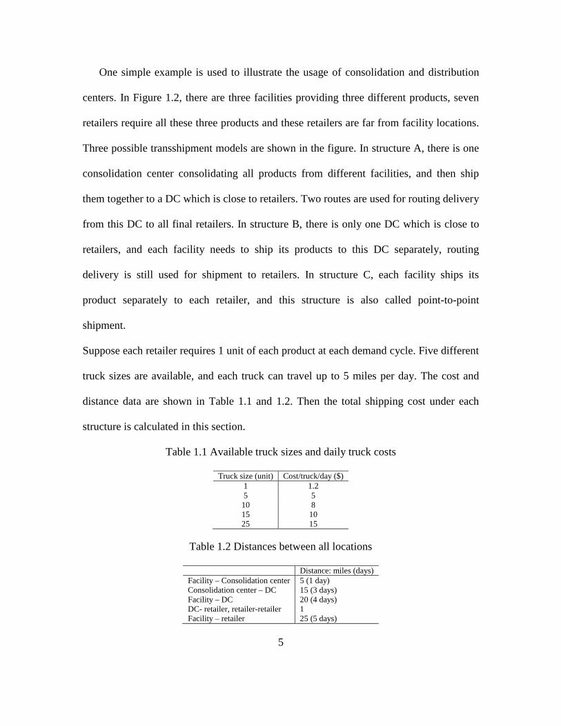
One simple example is used to illustrate the usage of consolidation and distribution

centers. In Figure 1.2, there are three facilities providing three different products, seven

retailers require all these three products and these retailers are far from facility locations.

Three possible transshipment models are shown in the figure. In structure A, there is one

consolidation center consolidating all products from different facilities, and then ship

them together to a DC which is close to retailers. Two routes are used for routing delivery

from this DC to all final retailers. In structure B, there is only one DC which is close to

retailers, and each facility needs to ship its products to this DC separately, routing

delivery is still used for shipment to retailers. In structure C, each facility ships its

product separately to each retailer, and this structure is also called point-to-point

shipment.

Suppose each retailer requires 1 unit of each product at each demand cycle. Five different

truck sizes are available, and each truck can travel up to 5 miles per day. The cost and

distance data are shown in Table 1.1 and 1.2. Then the total shipping cost under each

structure is calculated in this section.

Table 1.1 Available truck sizes and daily truck costs

Truck size (unit) Cost/truck/day ($) 1 1.2 5 5 10 8 15 10 25 15

Table 1.2 Distances between all locations

Distance: miles (days) Facility – Consolidation center 5 (1 day) Consolidation center – DC 15 (3 days) Facility – DC 20 (4 days) DC- retailer, retailer-retailer 1 Facility – retailer 25 (5 days)

6

Structure A

• Facility-Consolidation center: since each retailer requires 1 unit for each product

and there are 7 retailers in total, the total demand for each product is 7, the truck

with size 10 units is selected for transportation. The shipping cost = 3 (trucks) * 8

(daily truck cost) * 1 (day) = $24.

• Consolidation center-DC: the consolidation center consolidates all demand (21

units in total), thus the truck with size 25 units is selected for transportation. The

shipping cost = 1 (truck) * 15 (daily truck cost) * 3 (days) = $45.

• DC-retailer: two routes are used for routing delivery as shown in the Figure 1.1.

For the first vehicle, the total demand = 3*3 = 9, the truck with size 10 units are

selected for transportation, and the total shipping distance is 4 miles (1 day), thus

the shipping cost = 1 (truck) * 8 (daily truck cost) * 1 (day) = $8. For the second

vehicle, the total demand = 3*4 = 12, the truck with size 15 units are selected for

transportation, and the total shipping distance is 5 miles (1 day), thus the shipping

cost = 1 (truck) * 10 (daily truck cost) * 1 (day) = $10.

Under this transportation structure, the total shipping cost = 24 + 45 + 8 + 10 = $87.

Structure B

• Facility- DC: the truck with size 10 units is selected for transportation. The

shipping cost = 3 (trucks) * 8 (daily truck cost) * 4 (days) = $96.

• DC-Retailer: this is the same case as in structure A. For the first vehicle, the

shipping cost = 1 (truck) * 8 (daily truck cost) * 1 (day) = $8. For the second

vehicle, the shipping cost = 1 (truck) * 10 (daily truck cost) * 1 (day) = $10.

7

Under this transportation structure, the total shipping cost = 96 + 8 + 10 = $114.

Structure C

• Facility-Retailer: since each retailer only requires 1 unit for each product, the

smallest truck is selected for transportation. For each facility-retailer pair, the

shipping cost = 1 (truck) * 1.2 (daily truck cost) * 5 (days) = $6.

Under this transportation structure, the total shipping cost = 21 (pairs) * 6 = $126.

As noticed, total shipping cost under structure A with consolidation and distribution

centers is smaller than the other two structures. Even it costs to build consolidation and

distribution centers, the transportation savings may overcome the location cost if the

number of retailers and demand amount is large. In addition, having extra

consolidation/distribution centers will make the management easier and efficient, and it

will also overcome demand uncertainty and share risks in real business. In this

dissertation, several models are developed for assisting in planning supply distribution

including when and where to build consolidation and distribution centers.

The remaindert of this dissertation is as follows: Chapter 2 contains a detailed

literature review of several widely studied subproblems relevant to the integrated

approach taken in this dissertation. This includes the facility location, inventory

management and vehicle routing problems. In Chapter 3 an integrated network structure

including transshipment between DCs is considered. The transshipment is allowed

between DCs to provide the functions of both consolidation and distribution. A

transshipment network is a realistic representation of many real world problems that have

8

a general network structure with many supply/demand points and interconnecting links.

While becoming more complicated, it has important applications in industries. The

routing delivery strategy is also generally used in industries to take the advantages of Full

Truck Load (FTL), especially when served customers are close together and each

individual demand is small compared to the routing vehicle’s capacity. A mathematical

model will be presented and nonlinear terms are introduced to better represent the actual

system cost. However, due to the complexity of the problem, only small instances can be

solved directly from the mathematical model. Considering problem complexity and

recognizing costs are estimated and in reality other dynamically variables, a two-phase

solution methodology is proposed at the end of Chapter 3. Chapter 4 and 5 describe

detailed problems under each phase, heuristics for each phase problem are proposed and

tested as well. Chapter 6 solves and analyzes the integrated problem by using heristics

proposed in Chapter 4 and 5.

In Chapter 7, another innovation structure to group products into different sets based

on environmental or other factors is considered. Consolidation is allowed for shipping

products in the same product set, but products from different product sets must be

shipped separately. A mathematical model is derived here, two versions of a greedy

heuristic as well as a genetic algorithm are proposed and tested in this chapter.

Chapter 8 concludes my dissertation work and points out several possible future

research directions.

9

2. LITERATURE REVIEW

In this Chapter, a background review for each previously separate area in an integrated

supply chain network design problem is provided. Since there is a vast amount of

literature on these topics, references mentioned below are only examples to highlight

some of the results.

2.1 Facility Location Problem (FLP)

Modeling and solving FLP is a key element in strategic planning. It has its roots in the

pioneering work of Weber (1909) who considered the Fermat-Weber problem of locating

single facility to minimize the total travel distance between the site and a set of customers.

High costs associated with property acquisition and facility construction make facility

location or relocation projects long-term investments, and many other contributing

factors such as actual road network and congestion, customer response time demands and

dynamic customer bases complicate site selection and facility design. Cornuejols et al.

(1991), Sridharan (1995), Owen and Daskin (1998) and Melo et al. (2009) presented

summaries of FLP. More details about general characteristics in FLP can be found in

these papers.

Traditional FLP only considers fixed location cost and linear point-to-point

transportation cost (Albareda-Sambola et al., 2009; Averbakh et al., 2007; Harkness and

ReVelle, 2003; Hinojosa et al., 2000; Holmberg et al., 1999; Mazzola and Neebe, 1999;

Pirkul and Jayaraman, 1998; Snyder and Daskin, 2005). A basic fixed charge capacitated

plant location problem was formulated by Efroymson and Ray (1966). This paper

provided an integer-programming method for solving the plant location problem and a

10

branch-bound algorithm was then used to solve the problem. Daskin, Ozsen and Shen are

among the early authors who consider inventory control in FLP. They published several

papers in the past ten years about FLP with inventory considerations (Daskin, et al., 2002;

Ozsen et al., 2008; Qi and Shen, 2005; Sourirajan et al., 2007; Sourirajan et al., 2009) in

which they used risk-pooling to represent safety stock at DCs and used Lagrangian

relaxation based branch and bound heuristic to solve proposed mathematical formulations.

There are also a few papers discussing the location–routing problem. Min et al. (1998),

and Nagy and Salhi (2007) surveyed and classified this problem.

Among the available research, the multiple product case (Hinojosa et al., 2000;

Mazzola and Neebe, 1999; Melo et al., 2005; Santoso et al., 2005; Yao et al., 2010; Melo

et al., 2012) has received limited attention. There may be two reasons for this: the multi-

product problem can be translated to a single product problem based on an independence

assumption (demand, production, distribution and storage of each product is independent

from other products) and the complexity of multiple product problem.

The complexity of FLP has also limited much of the facility location literature to

simplified static and deterministic models. The first paper, published by Ballou (1968),

recognized the limited application of static and deterministic location models. More

papers appeared later to discuss FLP and the supply chain design problem under

uncertainty scenarios (Santoso et al., 2004; Qi and Shen, 2007).

2.2 Inventory Control Problem (ICP)

Inventory is required at one or more locations within a system to protect against shortages

resulting from random events and to allow rapid response to demand. Inventory also

11

exists due to the movement of economic load sizes in batch quantities different than unit

consumption. Inventory models seek to balance the costs of setups, inventory holding and

opportunity costs, shortages, and obsolescence.

An extensive body of literature has appeared in the past fifty years dating back to

Clark and Scarf (1960) on periodic and continuous review, deterministic and stochastic,

and single and multistage models. Silver et al. (1998) and Zipkin (2000) are two well-

known books which provide a thorough introduction about inventory modeling and

planning in operations research/management.

Within the ICP, the Economic Order Quantity (EOQ) model and its variants are

classical models for constant demand rate products. Power-of-two inventory policy is

widely used in multi-echelon inventory models, Roundy (1986) introduced the power-of-

two policies and he presented a 98% effective power-of-two policy for a one-warehouse,

multi-retailer inventory system with constant demand rate.

Risk pooling is an important concept in supply chain management. Risk pooling

suggests that demand variability is reduced if one aggregates demand across locations

because as demand is aggregated across different locations, it becomes more likely that

high demand from one customer will be offset by low demand from another. This

reduction in variability allows a decrease in safety stock and therefore reduces average

inventory. For example: in the centralized distribution system, the warehouse serves all

customers, which leads to a reduction in variability measured by either the standard

deviation or the coefficient of variation. Thus, risk-pooling is often used for modeling

optimal safety stock level when demand is stochastic.

12

Traditional ICP research focuses on a constant demand rate or general distributions

for demand and constant unit transportation rate (Miranda and Garrido, 2009; Pourakbar

et al., 2007). Nenes et al. (2010) built an inventory-review system for multiple

intermittent and lumpy products. Ertogral et al. (2007) considered two problems under

equal-size shipment policy with an all-unit-discount transportation cost structure. Tagaras

and Vlachos (2001) considered a periodic review inventory system with two

replenishment modes: regular orders and emergency orders. Schmitt et al. (2010)

invested an inventory system with stochastic demand and supply.

Excluding inventory holding at some physical locations, cross-docking operations

were first pioneered in the U.S. trucking industry in the 1930s. Cross-docking is done by

moving cargo from one transport vehicle directly into another, with minimal or no

warehousing. Waller et al. (2006) analyzed the impact of cross-docking on inventory in a

decentralized retailer supply chain. Retailers such as Wal-Mart have built efficient

systems with rapid replenishment to such a competitive advantage with sale information

and cross-docking (Apte and Viswanathan, 2000).

Another innovation is Vendor-Managed Inventory (VMI) control system. VMI is a

family of business models in which the buyer of a product (business) provides certain

information to a vendor (supply chain) supplier of that product and the supplier takes full

responsibility for maintaining an agreed inventory of the material, usually at the buyer's

consumption location (usually a store). A third-party logistics provider can also be

involved to make sure that the buyer has the required level of inventory by adjusting the

demand and supply gaps (Franke, 2010).

13

One of the keys to making VMI work is shared risk. In some cases, if the inventory

does not sell, the vendor (supplier) will repurchase the product from the buyer (retailer).

In other cases, the product may be in the possession of the retailer but is not owned by the

retailer until the sale takes place, meaning that the retailer simply houses (and assists with

the sale of) the product in exchange for a predetermined commission or profit (sometimes

referred to as consignment stock). This is also one of the successful business models used

by Wal-Mart and many other big box retailers.

2.3 Vehicle Routing Problem (VRP)

In its basic form, VRP is “to determine K vehicle routes, where a route is a tour that

begins at the depot, traverses a subset of the customers in a specified sequence and

returns to the depot. Each customer must be assigned to exactly one of the K vehicle

routes and total size of deliveries for customers assigned to each vehicle must not exceed

the vehicle capacity. The routes should be chosen to minimize total travel cost” (Fisher,

1995). Golden (1988) was a one of the first to summarize the theory and practice of VRP

in a book. Gendreau et al. (1996) provided a review of contributions to the VRP with

stochastic demands. A recent review is provided by Laporte (2009) who categorized and

summarized the main contributions during these years as: exact algorithms, classical

heuristics, and meta-heuristics.

There are three popular variants of VRP: Vehicle Routing Problem with Pickup and

Delivery (VRPPD) in which a number of goods need to be moved from certain pickup

locations to other delivery locations (Ai and Kachitvichyanukul, 2009; Berbeglia et al.,

2012; Hoff et al., 2009; Subramanian et al., 2010); Vehicle Routing Problem with Time

14

Windows (VRPTW) in which the delivery locations have time windows within which the

deliveries (or visits) must be made (Berger and Barkaoui, 2004; Li, 2008); and

Capacitated Vehicle Routing Problem (with or without Time Windows) (CVRP or

CVRPTW) in which the vehicles have limited carrying capacity of the goods that must be

delivered (Lin et al., 2009; Toth and Tramontani, 2008; Yurtkuran and Emel, 2010). In

addition, stochastic version problem (Dynamic real time VRPs) has also been studied

(Pillac, et al., 2012).

The Inventory Routing Problem (IRP) can be interpreted as an enrichment of VRP to

include inventory concerns. The inventory component arises because customers consume

product over time and have only limited storage capacity. The presence of inventory

complicates the routing decisions in two fundamental ways. First, the storage capacity

has to be taken into account when deciding on delivery quantities. Second, inventory

holding costs may be incurred which has to be accounted for in the objective function

(Bertazzi et al. 2008).

The first papers on IRPs appeared in 1980s (Dror and Ball, 1987; Dror et al., 1985,

Federgruen and Zipkin, 1984; Golden et al., 1984; Hall, 1985.) Then there are a varied

class of papers discussing IRP applications and solution approaches (Archetti et al., 2007;

Bard et al., 2010; Bartazzi et al., 2002; Huang and Lin, 2010; Li et al., 2010; Li et al.,

2011; Moin, et al., 2011; Shu et al., 2005; Solyah et al., 2012; Yu et al., 2008;

Zachariadis, et al., 2009; Zhao et al., 2008; Zhao et al., 2007;), also about performance

analysis (Anily and Bramel, 2004; Li et al., 2010).

15

2.4 Integrated Supply Chain

Numerous books and papers have been published on SCM covering many issues and

problem environments. However, as noted above, most research only focuses on some

particular issues and few models comprehensively address the integrated network. To

achieve a global optimal (or near optimal) solution, it is necessary to consider the entire

system in an integrated fashion and include all trade-offs in a realistic fashion.

When designing supply chains, firms are often faced with the competing demands of

improved customer service and reduced cost. In general, the higher the customer

responsiveness required, the higher the total cost needed. Nozick and Turnquist (2001),

and Shen and Daskin (2005) considered the trade-off between service level and cost in an

integrated supply chain.

Two research papers are found to have considered all three problems in a supply

chain. Shen and Qi (2007) proposed a model incorporating inventory and routing costs in

strategic location problem in a three-level supply chain. However, they just used an

approximate function for the routing stage instead of considering details and real routing

decisions. Javid and Azard (2010) extended Shen and Qi (2007) to include routing

decisions in their model, but they fixed routing frequency in their model and use them as

an input parameter. Both papers only considered a single-product system.

A summary table for most related journal papers referred in this dissertation is shown

as in Table 2.1. The table classifies papers by type of demand (deterministic or

stochastic), whether location (L), transportation (T), inventory (I) and routing (R)

decisions were considered, and also the main solution methods used in each paper.

16

Table 2.1 Related literature review summary

Author (year) Product Demand L T I R Main solution method Albareda-Sambola et al. (2009)

N/A N/A X X

Lagrangian relaxation

Averbakh et al. (2007)

N/A N/A X X

Dynamic programming

Bidhandi and Yusuff (2010)

Multiple Deterministic X X

Sample average approximation, Benders’ decomposition

Elhedhli and Gzara (2008)


Lagrangian relaxation, interior point cutting plane methods, primal heuristics

Harkness and ReVelle (2003)

Single Deterministic X X

Mixed integer programming

Hinojosa et al. (2000)



Holmberg et al. (1999)

N/A N/A X X


Mazzola and Neebe (1999)



Pirkul and Jayaraman (1998)



Santoso et al. (2005)


Sample average approximation, bender's decomposition

Snyder and Daskin (2005)

Single Stochastic X X


Ertogral et al. (2007)

Single Deterministic

X

Analytic method

Nenes et al. (2010) Multiple Stochastic

X

Analytic method Pourakbar et al. (2007)

Multiple Deterministic

X

Genetic algorithm

Schmitt et al. (2010)

Single Stochastic

X

Analytic method

Gebennini et al. (2009)

Single Stochastic

X X

Recursive heuristic algorithm

Lee et al. (2008) Single Deterministic

X X

Decomposition and post-improvement Ai and Kachitvichyanukul (2009)


X Particle swarm optimization algorithm

Berger and Barkaoui (2004)


X Genetic algorithm

Gutiérrez-Jarpa et al. (2010)


X Column generation, Label-setting algorithm, Branch and Bound

Ho et al. (2008) Single Deterministic

X Genetic algorithm

Hoff et al. (2009) Single Deterministic

X Tabu Search

Lin et al. (2009) Single Deterministic

X Simulated annealing, Tabu search Marinakis et al. (2010)


X Hybrid particle swarm optimization algorithm

Nagy and Salhi (2005)


X Heuristic algorithm

Subramanian et al. (2010)


X Parallel algorithm, variable neighborhood descent procedure, iterated local search

Yurtkuran and Emel (2010)


X Hybrid electromagnetism-like algorithm

Chan et al. (2001) Single Stochastic X

X Priori (space-filling curve) and posteriori (extended Clarke-Wright procedure) optimization

17

Author (year) Product Demand L T I R Main solution method Anily and Bramel (2004)


X X Fixed partition policies

Archetti et al. (2008)


X X Branch-and-Cut

Bard and Nananukul (2010)


X X Branch-and-price

Bertazzi et al. (2002)


X X Heuristic algorithm

Huang and Lin (2010)

Single Stochastic

X X Ant colony optimization algorithm

Li et al. (2010) Single Deterministic

X X Analytic method

Li et al. (2011) Single Deterministic

X X Decomposition solution approach based on a fixed partition policy

Moin et al. (2011) Multiple Deterministic

X X Genetic algorithm

Shu et al. (2005) Single Stochastic

X X Column generation algorithm Solyalı et al. (2012)

Single Stochastic

X X Branch and Cut

Yu et al. (2008) Single Deterministic

X X Lagrangian relaxation Zachariadis et al. (2009)


X X Local search heuristic algorithm

Zhao et al. (2008) Single Deterministic

X X Variable large neighborhood search algorithm

Daskin et al. (2002)

Single Stochastic X X X


Erlebacher and Meller (2000)

Single Deterministic X X X

Heuristic algorithm

Liu et al. (2010) Single Stochastic X X X


Melo et al. (2005) Multiple Deterministic X X X


Melo et al. (2012) Multiple Deterministic X X X

Tabu search Miranda and Garrido (2004)



Miranda and Garrido (2008)



Miranda and Garrido (2009)


Heuristic algorithm

Nozick and Turnquist (2001)

N/A N/A X X X


Ozsen et al. (2008) Single Stochastic X X X

Lagrangian relaxation Qi and Shen (2007)



Shen and Daskin (2005)


Genetic algorithm

Shen and Honda (2009)



Sourirajan et al. (2007)



Sourirajan et al. (2007)


Genetic algorithm

Yao et al. (2010) Multiple Stochastic X X X

Recursive heuristic algorithm Javid and Azad (2010)

Single Stochastic X X X X Tabu Search and Simulated Annealing

Shen and Qi (2007)

Single Stochastic X X X X Lagrangian relaxation

L: Location; T: Transportation; I: Inventory; R: Routing

18

There are several contributions of this dissertation research: First of all, an integrated

optimization framework is proposed for a multi-product supply chain network. There is

limited research discussing multi-product supply chain optimization problems, especially

considering product-mix during transportation and transshipments. However, multi-

product supply chain network is much more realistic: big retailers such as Wal-Mart

handle thousands of different products. Jointly considering ordering, distribution and

storage of multiple products will allow taking the advantage of full-truck-load shipments,

economies-of-scale, risk-pooling, etc. In this framework, DC location, allocation,

capacity, transportation, inventory and routing decisions in the whole system will be

optimized simultaneously. Second, a new network structure including transshipment

between DCs is considered in the model. Third, when minimizing total system cost, some

nonlinear terms are introduced to better represent the actual system cost. Fourth, a routing

delivery strategy is used to serve retailers from DCs. To take the advantage of full-truck

load, retailers are grouped into routes and one vehicle is assigned to serve multiple

retailers in the same route at an optimal joint frequency. Finally, several effective

heuristics are proposed for this integrated optimization problem.

19

3. PROBLEM DESCRIPTION

In this research, an integrated three-echelon multi-product supply chain network design

problem is considered which includes multiple production facilities (plants), DCs and

retailers. Each plant supplies one type of product and retailers have stochastic demand

requirements for these products. Each plant ships its finished products to one or more

DCs which are also called its corresponding Plant Warehouses (PWs). DCs combine

different products from different PWs and then ship mixed products to their assigned

retailers. Retailers are randomly clustered in a service region so a routing delivery

strategy is used to ship products from DCs to retailers. The goal of this research is to

select locations for DCs and determine transportation assignment, set inventory policy

based on service requirements, and to schedule vehicle routes to meet customers’ demand

such that the total cost in the system is minimized.

This three-echelon supply chain network is simplified from a four-echelon supply

chain network which exists in many real business situations. In a four-echelon supply

chain, production facilities supply multiple different products, shipments from one or

more production facilities are stored or just cross-docked at consolidation centers for

distribution. Regional warehouses then receive bulk shipments for subsequent delivery to

retailer outlets. The three-echelon research problem performs the same functions by

considering transshipments between DCs.

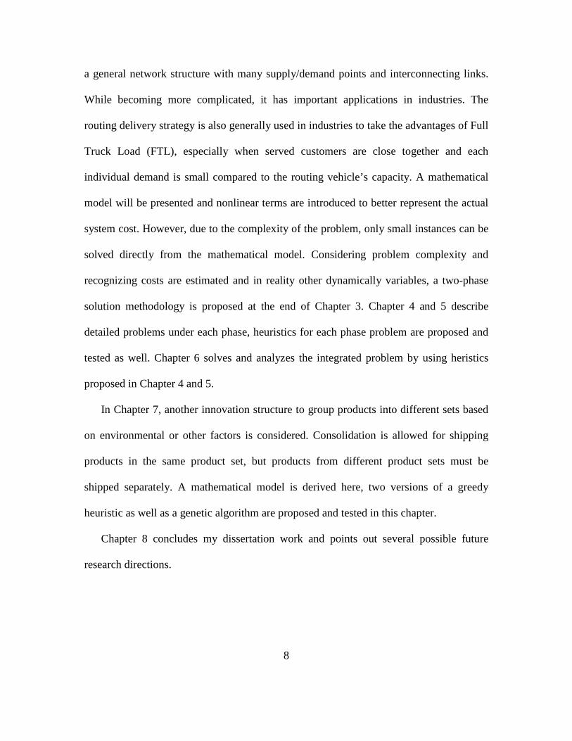
Figure 3.1 shows a four-echelon supply chain network as well as a three-echelon

supply chain network problem which will be discussed in this dissertation. Products flow

along shipment arcs, generally from left to right starting at production facilities and then

going through one or more distribution centers prior to being delivered to the final

20

customer. DCs in the proposed system have the functions of both consolidation and

distribution, and opened DCs receiving finished product directly from plants are called

plant warehouses (PWs). Transhipments occur between distribution centers where a DC

serves end customers but is not a PW. In addition, there are transshipments between DCs

to combine different products.

Figure 3.1 Integrated problem and solution example

In this network, cost components considered include fixed cost of locating DCs,

direct shipping cost from plants to its PWs and transshipment cost between DCs, working

inventory and safety stock holding cost at DCs and retailers, and routing cost from DCs

to retailers.

3.1 Assumptions and Decisions

Assumptions used in this dissertation and related decisions solved by the proposed

framework are provided in this section.

Assumptions

1. Each plant supplies a different type of product.

DistributionCenterDistributionCenter RetailerConsolidationCenterFacility

1

2

3

3

2

1

6

5

4

9

8

7

RetailerFacility

1

2

3

3

2

1

3

2

1

6

5

4

9

8

7

21

2. Potential locations for DCs are known and different capacity level options are

available for each DC at each location.

3. Retailers are randomly clustered across the service region. Routing delivery strategy

is used to ship products from DCs to retailers. Each DC owns a homogenous fleet of

vehicles, deliveries are made that begin and end their runs at each DC.

4. Demand of each type of product at each retailer per period follows a known stationary

distribution (assumed to be the normal distribution later). Demands between different

types of product and retailers are independent.

5. Single source: all products at one retailer should be delivered by one DC.

6. Single path: each plant ships its finished product to its PWs, and then PWs deliver

products to retailers assigned to them by routing delivery and other DCs by

transshipment. Only one path is allowed for each type of product at each retailer. This

path may be Plant-PW-Retailer or Plant-PW-DC-Retailer.

7. Both working inventory and safety stock inventory are held at DCs and retailers.

8. The same service level constraint applies to all products at all retailers.

9. Full truck load (FTL) shipping is used from plants to DCs and between DCs, but

multiple truck size choices may exist.

Decisions

1. Location and capacity decisions: how many DCs to locate, where to locate them, and

what capacity level to locate for each opened DC.

2. Allocation decisions: assignments of PWs for plants and DCs for retailers.

22

3. Transportation decisions: truck size selection for delivery from plants to PWs and

transshipments.

4. Routing decisions: how to build vehicle routes starting from DCs to serve retailers,

and routing frequencies of deliveries to retailers.

3.2 Problem Formulation

A mathematical formulation of the problem is presented as follows:

Index sets

P set of plants

I set of retailers

J set of potential DCs

K set of available DC capacity levels

L set of available truck size levels

N set of available routing frequencies

V set of tours

Parameters

zα left α-percentile of standard normal random variable Z

Miv Auxiliary variable defined for retailer i for subtour elimination in route of

vehicle v

PWp number of PWs allowed for plant p

µpi mean of annual demand of product p at retailer i

σ2pi variance of annual demand of product p at retailer i

23

Cjk capacity for DC j at level k

fjk annualized fixed cost if DC j is opened at capacity level k

ql truck size at level l

astl fixed cost of one FTL at size level l from node s to node t

bstl unit shipping cost from node s to node t

ltst lead time from node s to node t

hps annual holding cost of product p per unit at point storing point s

D routing distance limit per trip

q routing vehicle’s capacity

dst distance from node s to node t

s speed of the default vehicle

a fixed cost of using one routing vehicle at DCs

c unit routing delivery cost per mile

fn routing frequency at level n

Decision Variables

Ojk 1 if opening a DC at location j at capacity level k, 0 otherwise

Tstl 1 if using truck size at level l for FTL from node s to node t, 0 otherwise

Wpj 1 if DC j is a PW for production facility p, 0 otherwise

Xstv 1 if s immediate precedes t in route v, 0 otherwise

Yji 1 if retailer i is assigned to DC j, 0 otherwise

Ypjj’i 1 if retailer i obtains product p through path p-j-j’-i , 0 otherwise

Rvi 1 if use route v to supply demand at retailer i, 0 otherwise

24

Zvn 1 if route v has routing frequency at level n, 0 otherwise

Ipj’j 1 if DC j receives product p from DC j’ (a PW for product p), 0 otherwise

To simplify the notation, let:

v n vnn Nf Zγ

∈=∑ the number of trips for route v in one year

,v st stvs t I Jd d X

∈=∑ U

the distance of route v

1 v viv Vi

v viv V

d Rlt

R sγ∈

∈

= +∑∑

the lead time for the retailer i. Lead time is a

function of route frequency (first component) and route distance (second component).

Risk exposure to demand variability at a minimum occurs due to the duration of time

between deliveries plus time along the route for a retailer. For example, if a route

starts every hour and a retailer is 15 minutes into a route then when the order is

placed and the truck leaves the DC at 8:00am, the retailer’s inventory position must

be sufficient to accommodate demand until 9:15am since that is the earliest time they

can receive another shipment. Any required preordering time prior to truck departure

would need to be added onto this lead time.

3.2.1 Cost Components

• FC: Annualized fixed cost of locating DCs:

, jk jkj J k KFC f O

∈ ∈=∑ (3-1)

• IRC: Inventory routing cost from DCs to retailers:

( )0.5 pip P

v v pi pi iv V i I p P v Vvi vv V

a cd h z ltR α

µγ σ

γ∈

∈ ∈ ∈ ∈∈

+ + +

∑∑ ∑ ∑ ∑∑

(3-2)

25

IRC includes truck’s routing cost and inventory holding cost. The first component

of equation (3-2) is the annual routing cost. Each shipment contains a fixed cost (a)

and a variable cost (cdv), which are multiplied by the number of shipments per time

(year). The variable cost is linear function over the route distance dv. The second

component of equation (3-2) is the annual inventory cost which includes both regular

inventory and safety stock inventory. The regular inventory level is half of each-time

delivery amount and the safety stock level is related to delivery lead time as discussed

above with the appropriate service level specified on the lead time demand

distribution..

• SC: Shipping cost. Let Qpj be the annual shipping quantity from Plant p to DC j

and Qpj’j be the annual transshipment quantity of product p from DC j’ to DC j,

then showing by equation (3-3):

' 'pjj pi pjj ii IQ Yµ

∈=∑ and ''pj pjjj J

Q Q∈

=∑ (3-3)

Let qpj be the truck size used for direct shipping from Plant p to DC j , qj’j be the

truck size for transshipment from DC j’ to DC j, and let Apj , Aj’j be the shipping

cost for one FTL from Plant p to DC j and between DC j’ to DC j, then:

' ' pj l pjl j j l j jll L l Lq qT q qT

∈ ∈= =∑ ∑ (3-4)

( ) ( )' ' ' ' pj pjl pjl l pjl j j j jl j jl l j jll L l LA a b q T A a b q T

∈ ∈= + = +∑ ∑ (3-5)

'

'' , ''

pj jpj p Pj pj j jp P j J j j

pj j j

jj J

QQSC A A

q q

SC SC

∈

∈ ∈ ≠

∈

= +

=

∑∑ ∑

∑ (3-6)

26

• Tstl is a binary variable whether a truck size at level l is selected for the FTL from

node s to node t. Then equation (3-4) selects the optimal truck size for direct

shipping from Plant p to DC j and equation (3-5) is the optimal one FTL shipping

cost from Plant p to DC j (Apj) and between DC j’ to DC j (Aj’j ). Total annual

shipping cost from plants and other DCs to DC j is presented in equation (3-5)

and equation (3-6) is tha total annual shipping cost for all DCs. SSC: Safety stock

inventory holding cost at DCs. Note that safety stock must accommodate lead

time demand uncertainty. For each DC, its safety stock includes two parts: (1)

safety stock for shipping from plants, (2) safety stock for transshipment from

other DCs. The proposed model could be modified if replacement lead time or

demand is more accurate. If using risk pooling method, then the safety stock at

each DC j is:

( )2 2' ' ', ' '

,

pj pj pi pjj i j j pi pj jii I j J j J i I

pj pjp P j J

SS z lt Y lt Y

SSC h SS

α σ σ∈ ∈ ∈ ∈

∈ ∈

= +

=

∑ ∑ ∑∑

(3-7)

Equation (3-7) provides safety stock against the aggregated demand variability at

DC j. Depending on the exact ordering policy for DCs from plants and other DCs,

this expression coubld be modified.

• RIC: Regular inventory holding cost at DCs. For each DC, it receives products

either through plants directly or through transshipment from other DCs. Since

FTL is used for both cases, the Regular Inventory (RI) level of product p at DC j

is:

27

' '

' , ''

,

2 2pj j j pj j

pj j J j jpj jp P

pj pjp P j J

q q QRI

Q

RIC h RI

∈ ≠∈

∈ ∈

= +

=

∑ ∑∑

(3-8)

3.2.2 Mixed Integer Programming Model

Using the cost terms defined in the previous section, the system decision problem can be

formulated as a mixed integer mathematical programming model. The formulation is as

follows:

Minimize ( FC + IRC + SC + SSC + RIC ) (3-9)

Subject to:

1 viv VR i I

∈= ∀ ∈∑ (3-10)

, pi vip P i I

v

Rq v V

µ

γ∈ ∈ ≤ ∀ ∈

∑ (3-11)

vd D v V≤ ∀ ∈ (3-12)

( )| | | | 1 , ,sv tv stvM M I X I s t I v V− + × ≤ − ∀ ∈ ∈ (3-13)

,stv tsvs I J s I JX X t I J v V

∈ ∈= ∀ ∈ ∈∑ ∑U U

U (3-14)

,1 jivi I j J

X v V∈ ∈

≤ ∀ ∈∑ (3-15)

( ) 1 , ,itv jtv jit I JX X Y i I j J v V

∈+ ≤ + ∀ ∈ ∈ ∈∑ U

(3-16)

,itv vit I JX R i I v V

∈= ∀ ∈ ∈∑ U

(3-17)

1 jkk KO j J

∈≤ ∀ ∈∑ (3-18)

28

( )' ', ' , ' pi ji j i pjj jk jkp P i I j J j j k K

Y Y I C O j Jµ∈ ∈ ∈ ≠ ∈

+ ≤ ∀ ∈∑ ∑ ∑ (3-19)

1 vnn NZ v V

∈= ∀ ∈∑ (3-20)

pj pj JW PW p P

∈≤ ∀ ∈∑ (3-21)

''| | ,pjj pjj J

I J W p P j J∈

≤ ∀ ∈ ∈∑ (3-22)

1 ,pjll lT p P j J

∈≤ ∀ ∈ ∈∑ (3-23)

' 1 , ' , 'jj ll LT j j J j j

∈≤ ∀ ∈ ≠∑ (3-24)

' ', , , , , , , , {0,1}

, , ' , , , , , , ,jk vi stv ji vn pj pjl jj l pjjO R X Y Z W T T I

i I j j J p P k K s t I J v V n N l L

∈

∀ ∈ ∈ ∈ ∈ ∈ ∈ ∈ ∈U (3-25)

0 ,ivM i I v V≥ ∀ ∈ ∈ (3-26)

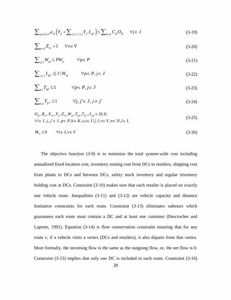
The objective function (3-9) is to minimize the total system-wide cost including

annualized fixed location cost, inventory routing cost from DCs to retailers, shipping cost

from plants to DCs and between DCs, safety stock inventory and regular inventory

holding cost at DCs. Constraint (3-10) makes sure that each retailer is placed on exactly

one vehicle route. Inequalities (3-11) and (3-12) are vehicle capacity and distance

limitation constraints for each route. Constraint (3-13) eliminates subtours which

guarantees each route must contain a DC and at least one customer (Descrocher and

Laporte, 1991). Equation (3-14) is flow conservation constraint ensuring that for any

route v, if a vehicle visits a vertex (DCs and retailers), it also departs from that vertex.

More formally, the incoming flow is the same as the outgoing flow, or, the net flow is 0.

Constraint (3-15) implies that only one DC is included in each route. Constraint (3-16)

29

links the retailer-DC allocation and the routing components of the model. For each

retailer i, it is assigned to DC j if the route v which visits it starts from DC j (Javid and

Azad, 2010). Constraint (3-17) links the retailer-route allocation and the routing

components of the model: retailer i is assigned to route v if the route v visits it. Constraint

(3-18) ensures that each DC can be assigned to only one capacity level. Constraint (3-19)

is capacity limitation for DCs, DC’s capacity is defined as the total product flow through

it, this constraint also ensures that opening one DC before any retailer or PW assigning to

it. Equality (3-20) is route frequency constraint and constraint (3-21) limits the number of

PWs for each plant. Constraint (3-22) links the transshipment and PW allocation: DC j is

a PW for production facility p if there is any DC receiving product p from DC j.

Constraints (3-23) and (3-24) are truck size selection for direct shipping and

transshipment. Constraint (3-25) and (3-26) are integrality and non-negativity restrictions

on the decision variables.

3.3 Solution Methodology

The proposed model is a large-scale optimization problem which includes both FLP and

IRP. In order to find a good feasible solution in a reasonable time, the original problem is

decomposed into two phases: In the first phase, an approximated IRC function is used to

locate DCs, and assign retailers and PWs to those opened DCs. In the second phase,

actual routing order and delivery frequency for each route will be determined.

30

4. PHASE I: MULTI-PRODUCT FLP WITH APPROXIMATED IRC

In this chapter, a FLP which focuses on locating DCs and assigning retailers is discussed.

Detailed routing decisions will not be considered here. An approximated routing cost

function representing distributions of retailer location and demand is developed to

provide insights into mathematical programing models.

4.1 Problem Description and Mathematical Formulation

A coefficient r ji is introduced in this phase to approximately represent the annual IRC at

retailer i if assigned to DC j. Then the approximated total inventory routing cost becomes:

, ji jii I j JIRC r Y

∈ ∈=∑ . This cost coefficient is approximated for each DC-retailer pair off-

line. Shen and Qi (2007) introduced a continuous approximation method in their paper,

but in their research, customers are uniformly scattered in a connected region and

location information for retailers are not included in the routing cost estimation. However,

routing strategy is a better strategy compared to direct shipping if customers are clustered

and close to each other, thus retailers are assumed to be clustered in the service region in

this research. The estimation of the routing coefficient r ji in this research considers real

location information for all retailers and potential DCs. To calculate this coefficient,

some new notation is introduced as follows:

αji routing cost using nearest neighborhood insertion method for retailer i

from DC j

βji direct shipping cost for retailer i from DC j

Rj(i) set of retailers in the route serving retailer i from DC j

31

Aj(i) set of arcs forming the route serving retailer i from DC j

nji number of retailers in the route serving retailer i from DC j, | Rj(i) |

∆ji distance per route trip serving retailer i from DC j

1. If retailer i is far away from DC j (the distance between them exceeds half of the

routing distance limit D), retailer i will not be possible to assigned to DC j:

0 if 2ji ji

DY d= ≥ .

2. For each DC j to its reachable retailer i, a modified inventory routing cost formulation

can be used to determine the routing cost from DC j to retailer i :

1min

2ji pi ji

ji n pi pip Pn Nji n n

a cf h z

n f f sα

µα σ

∈∈

+ ∆ ∆ = + + +

∑ (4-1)

Equation (4-1) utilizes the optimal routing frequencies from available frequencies to

minimize IRC. The cost function includes annualized individual routing delivery cost

(first component) and inventory holding cost (second component). The inventory at

retailer i includes regular inventory which is half of a delivery batch plus safety stock

which is related to routing delivery time. This formulation is similar as equation (3-2)

and detailed explanination is also similar as in equation (3-2).

An optimistic route is constructed using nearest neighborhood insertion method:

for retailer i, select as many neighbors as possible to form a route such that both

distance and capacity limits are satisfied. The process proceeds iteratively by

selecting the next nearest neighbor and then forming an optimal tour for selected set

32

of retailers in this route until no such a candidate retailer remains. This problem can

be formulated as:

max | ( ) |ji jn R i= (4-2)

( , ) ( ). .:

jji lml m A i

s t d D∈

∆ = ≤∑ (4-3)

( ), j

pm pm R i p P

ji

vq

µ

γ∈ ∈

≤∑

(4-4)

The objective function (4-2) is trying to maximize total number of retailers along

current route with route distance constraint (4-3) and truck capacity constraint (4-4).

3. If direct shipping method is used to serve retailer i from DC j, then the direct shipping

cost is:

( ) 21min 2

2pi ji

ji ji n pi pip Pn Nji ji

da cd f h z

sα

µβ σ

γ γ∈∈

= + + + +

∑ (4-5)

Equation (4-5) utilizes the optimal routing frequencies from available frequencies to

minimize IRC if retailer i receives deliveries from DC j individually.

4. The routing parameter r ji is estimated as the average of possible routing cost and

direct shipping cost as ( ) / 2ji ji jir α β= + . This average value is found in empirical

studies to more closely approximate solutions than αji alone. More discussion about

how to construct routing parameter r ji is referred to Chapter 6.

Integer Programming Model

By using the off-line calculated routing parameter r ji, the overall problem then becomes:

Minimize (FC + IRC + SC + SSC + RIC) (4-6)

33

Subject to:

1 jij JY i I

∈= ∀ ∈∑ (4-7)

'',1 ,pj jij j J

Y i I p P∈

= ∀ ∈ ∈∑ (4-8)

', ' ,pj ji jip P j J

Y MY i I j J∈ ∈

≤ ∀ ∈ ∈∑ (4-9)

', ' ,pjj i pji I j J

Y MW p P j J∈ ∈

≤ ∀ ∈ ∈∑ (4-10)

pj pj JW PW p P

∈≤ ∀ ∈∑ (4-11)

1 jkk KO j J

∈≤ ∀ ∈∑ (4-12)

1 ,pjll lT p P j J

∈≤ ∀ ∈ ∈∑ (4-13)

' 1 , ' , 'jj ll LT j j J j j

∈≤ ∀ ∈ ≠∑ (4-14)

', , , ' , ' pi ji pi pjj i jk jkp P i I p P i I j J j j k K

Y Y C O j Jµ µ∈ ∈ ∈ ∈ ∈ ≠ ∈

+ ≤ ∀ ∈∑ ∑ ∑ (4-15)

' ', , , , , {0,1} , , ' , , ,jk ji pj pjl jj l pjj iO Y W T T Y i I j j J p P k K l L∈ ∀ ∈ ∈ ∈ ∈ ∈ (4-16)

The objective function (4-6) is to minimize system-wide total cost. Constraints (4-7)

and (4-8) are single source and single path constraints. Constraints (4-9) link variables

Ypj’ji and Yji. Constraints (4-10) link the Ypj’ji transport path variables with the plant

warehouse variables Wpj to ensure initial receiving warehouses are opened. Constraint (4-

11) limits the number of PWs for each plant if desired. Constraint (4-12) means that at

most one DC with one capacity level can be built at each potential location. Constraints

(4-13) and (4-14) allow at most one type of truck being used for direct shipping and

34

transshipment between any plant-PW pair or DC-DC pair. Constraint (4-15) is the

capacity limitation for each DC, the capacity of one DC is measured by its total annual

flow, and this constraint also guarantees to open a DC if any retailer or PW is assigned to

it. Constraint (4-16) is the binary constraint for all binary decision variables.

4.2 Problem Analysis

In the current model, there are single source constraints for each retailer (4-7) and single

path constraints for each type of product at each retailer (4-8). To facilitate

implementation and solution, the optimality of these restrictions is examed. Assume first

that n > 1, and let PW(p) be the set of DCs which are PWs for product p. Consider the

following cases:

1. DC j is not a PW for product p, and j receives product p from several different PWs.

In other words, ( )j PW p∉ , 1 1 2 21 2 1 2 1 2 1 2, , , , , : 1, 1pj ji pj jij j j j j i i I i i Y Y∃ ≠ ≠ ∈ ≠ = = .

2. DC j is a PW for product p, but j still receives product p from other PWs. In other

words, ( )j PW p∈ , '' , : 1pj jij j i I Y∃ ≠ ∈ = .

Figure 4.1 Potential optimal network structure example

Figure 4.1 illustrates these two cases. In this figure, there are two plants providing

two different types of products and three opened DCs. PW(1) = {1, 2}, PW(2) = {1,3}.

DC3

DC2

DC1

P2

P1

35

In an optimal solution, may DC2 receive products 2 partially from DC1 and partially

from DC3 (Figure 4.2)? Or, may DC2 receive product 1 partially from DC1 even though

DC2 itself is a PW for product 1 (Figure 4.2)?

Figure 4.2 Two network structures

To simplify the problem, assume fixed cost of an opened DC is a continuous concave

function over the capacity level at this DC; holding rate, fixed and unit shipping cost are

the same, and there is no truck size limitation. Also assume annual demand standard

deviation (σ) equals coefficient of variation (cv) times demand (Q).

Theorem: There exists an optimal solution in which each opened DC j receives each type

of product p from only one PW under above assumptions.

To see how this theorem holds, these two cases are analyzed as follows.

Case 1: ( )j PW p∉

Structure A: DC j receives product p from DC j1 only with total quantity of Q.

Structure B: DC j receives product p partially from DC j1 with quantity of Q1 and

partially from DC j2 with quantity of Q2.

DC3

DC2

DC1

P1

P2

DC1

DC2

36

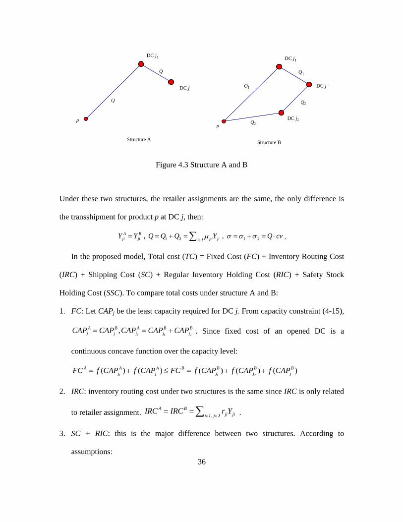
Figure 4.3 Structure A and B

Under these two structures, the retailer assignments are the same, the only difference is

the transshipment for product p at DC j, then:

1 2 1 2A Bji ji pi jii I

Y Y Q Q Q Y Q cvµ σ σ σ∈

= = + = = + = ⋅∑，， .

In the proposed model, Total cost (TC) = Fixed Cost (FC) + Inventory Routing Cost

(IRC) + Shipping Cost (SC) + Regular Inventory Holding Cost (RIC) + Safety Stock

Holding Cost (SSC). To compare total costs under structure A and B:

1. FC: Let CAPj be the least capacity required for DC j. From capacity constraint (4-15),

1 1 2,A B A B B

j j j j jCAP CAP CAP CAP CAP= = + . Since fixed cost of an opened DC is a

continuous concave function over the capacity level:

1 1 2( ) ( ) ( ) ( ) ( )A A A B B B B

j j j j jFC f CAP f CAP FC f CAP f CAP f CAP= + ≤ = + +

2. IRC: inventory routing cost under two structures is the same since IRC is only related

to retailer assignment. ,

A Bji jii I j J

IRC IRC r Y∈ ∈

= =∑ .

3. SC + RIC: this is the major difference between two structures. According to

assumptions:

DC j2

DC j

DC j1

DC j

DC j1

Q1

Q2

Q2

Q1

Q

Q

Structure BStructure A

pp

37

1 1

1 1

1 1

1 1

1 1

( ) ( ) ( )2 2

22 2

pj j jApj pj pj pj pj j j

pj j j

pj j jpj pjpj

pj j j

q qQ QSC RIC a b q a b q h h

q q

hq hqa Q a Qb Q

q q

+ = + + + + +

= + + + +

{ } ( )min ( ) 2 2Apj pjSC RIC a hQ b Q+ = +

Similarly, { } ( )1 2min ( ) 2 2 2Bpj pj pjSC RIC a hQ a hQ b Q+ = + +

1 2Q Q Q= + . Hence, ( ) ( )A BSC RIC SC RIC+ ≤ + .

4. SSC: Let ltst be the lead time from node s to node t, and σ be the standard deviation of

the demand variance, then the safety stock inventory holding cost at DCs:

( )( )

( ) ( )

1 1

1 1 2 2

1 1 2 2

1 1 2 2

2

Apj j j

Bpj j j pj j j

A Bpj j j pj j j

SSC hz lt lt

SSC hz lt lt lt lt

SSC SSC hz lt lt lt lt

α

α

α

σ σ

σ σ σ σ

σ

= +

= + + +

− = + − +

When DC j2 is closer to plant p and DC j, then the lead time is smaller compared to

DC j1, SSC under structure B is smaller. However, then it is better to receive

transshipment only from DC j2. Hence without loss of generality, assume

1 1 2 2pj j j pj j jlt lt lt lt+ ≤ + , then A BSSC SSC≤ .

As noticed, each cost component under structure A is smaller than under structure B,

hence structure B cannot exist in the optimal solution. However, the cost parameters in

the (SC+RIC) part is simplified assuming the holding rate, fixed and unit shipping cost

are the same, and no truck size limitation. Structure B may be better in some extreme

situations, and it is difficult to strictly exclude this situation mathematically. But this case

can be excluded by adding additional constraints if necessary.

38

Case 2: ( )j PW p∈

Structure C: DC j receives product p from DC j only with total quantity of Q.

Structure D: DC j receives product p partially from DC j’ with quantity of Q1 and

partially from DC j with quantity of Q2.

Structure E: DC j receives product p from DC j’ only with total quantity of Q.

Figure 4.4 Structure C, D and E

Using the same notation and argument process as in case 1:

1. FC: ,C D C EFC FC FC FC≤ ≤ .

2. IRC: C D EIRC IRC IRC= = .

3. SC + RIC:

{ }{ } ( ) ( ){ } ( )

1 1 2 2

min ( ) 2

min ( ) 2 2 2

min ( ) 2 2

Cpj pj

Dpj pj pj pj

Epj pj

SC RIC a hQ b Q

SC RIC a hQ b Q a hQ b Q

SC RIC a hQ b Q

+ = +

+ = + + +

+ = +

Hence, ( ) ( ) ,( ) ( )C D C ESC RIC SC RIC SC RIC SC RIC+ < + + < + .

pDC j p

p

DC j

DC j

DC j'

DC j'

DC j'

QQ2

Q1

QQ

Q1

Structure C Structure D

Structure E

39

4. SSC:

( )( )

( )( )

' 1 ' 1 2

' '

1 ' '

' '

Cpj

Dpj j j pj

Epj j j

C Dpj pj j j

C Epj pj j j

SSC hz lt

SSC hz lt lt lt

SSC hz lt lt

SSC SSC hz lt lt lt

SSC SSC hz lt lt lt

α

α

α

α

α

σ

σ σ σ

σ σ

σ

σ

=

= + +

= +

− = − +

− = − +

' 'pj pj j jlt lt lt≤ + , hence, ' 'pj pj j jlt lt lt≤ + and then: ,C D C ESSC SSC SSC SSC≤ ≤ .

Again, each cost component under structure C is the smallest under these three structures.

However, the cost parameters are simplified in assumptions. To exclude both cases, the

following additional constraints can be added to the original model.

• Single source for DCs: DC j receives each type of product p for all retailers assigned

to it from only one PW (this PW maybe DC j itself).

'' , '1 ,pj j pjj J j j

I W p P j J∈ ≠

+ = ∀ ∈ ∈∑ (4-17)

' ' , , ' , 'pj ji pj ji IY MI p P j j J j j

∈≤ ∀ ∈ ∈ ≠∑ (4-18)

Constraints (4-17) and (4-18) guarantee each DC receives each type of product from

only one source, either through plant directly or from only one PW. However, these

constraints are only effective if more than one PW is allowed. If PWp = 1,

transshipment between DCs for each type of product will be determined

automatically. The binary constraint (4-16) should be updated to include new binary

variables if these new constraints are added.

40

4.3 Single Plant Warehouse Case

One special case of the original problem is that only one PW is allowed for each plant

(PWp = 1). Each plant ships its product to its specified PW and all demand for such a

product is supplied directly or indirectly (through transshipment) from this PW. Note that

the plant may ship to other DCs or customers, however, they are outside the logistics

system and set of retailers in the system being considered. In this case, if DC j is the PW

for plant p, then its optimal truck size can be determined off-line since the total demand

from the plant is fixed as the total demand over all retailers. For direct shipping from

Plant p to DC j, select an optimal truck size such that direct shipping and regular working

inventory holding cost (DSRIC) is minimized as in equation (4-19):

( )min2

pii I lpj pjl pjl l pjp Pl

l

qDSRIC a b q h

q

µ∈

∈

= + +

∑ ∑ (4-19)

To update the model formulation, constraint (4-13) is eliminated.

For transshipment, a greedy method can be used to decide the truck size off-line:

1. For each retailer i, assign it to its closest candidate DC j. If DC j is not open, then

open it.

2. For each plant p, assign it to its closest DC j’ opened in step 1, then j’ is the PW for p.

3. Since there is only one PW for each plant in this case, transshipment decisions can be

determined by previous steps. This is a transshipment between DC j and j’ if either

DC j or j’ is a PW and the other serves a retailer.

41

For transshipment from DC j’ to DC j, select an optimal truck size such that

transshipment and regular working inventory holding cost (TSRIC) is minimized as in

equation (4-20):

( ) ' '' ' '

'

min2

pj jp P pj jlj j j jl j jl l pjp Pl

l pj jp P

Q QqTSRIC a b q h

q Q∈

∈∈

= + +

∑∑ ∑

(4-20)

If Q = 0, then use smallest truck for potential transshipment. And if j = j’ , transshipment

cost is zero. To update the model formulation, constraint (4-14) is eliminated.

As described, truck selection variables Tstl in this sub-problem can be estimated.

However, the model is still hard to solve directly. The complexity comes from two

nonlinear components: one is the safety stock which contains two square roots

( )2 2' ' ', ',pj pi pjj i j j pi pj jii I j J i I

lt Y lt Yσ σ∈ ∈ ∈∑ ∑ , the other is the regular working inventory

where a fraction exists'

' ''

:pj jpj j pi pj jii I

pj jp P

QQ Y

Qµ

∈∈

=

∑∑. If the holding rates for

different products are the same, the second nonlinear term simplifies and will not be a

problem. The safety stock can be solved iteratively. The safety stock formulation can be

modified as in equation (4-21) by introducing two coefficients ',pj pj jS S :

2 2 2 2' ' ', '

' , ''

pj pi pjj i j j pi pj jii I j J i Ipj j J j j

pj pj j

z lt Y z lt YSS

S S

α ασ σ∈ ∈ ∈

∈ ≠= +

∑ ∑∑ (4-21)

If coefficients ',pj pj jS S are the optimal safety stock: 2', 'pj pj pi pjj ii I j J

S z lt Yα σ∈ ∈

= ∑ ,

2' ' 'pj j j j pi pj jii I

S z lt Yα σ∈

= ∑ , then the solution solved from the modified linear objective

42

function subject to the constraints will be the same as the original non-linear model. In

general, the closer ',pj pj jS S is to the optimal safety stock, the closer the linear term is to

the optimal safety stock cost. A similar recursive procedure to that used in Gebennini et

al. (2009) based on the modified linear model is developed in order to find an admissible

solution with the following steps:

Set iter = 1. Set ',pj pj jS S to be 0.01.

1. Apply the new binary-integer linear model and find the solution.

2. For each type of product p and DC j where ', '0pjj ii I j J

Y∈ ∈

≠∑ or ' 0pj jii IY

∈≠∑ ,

calculate the actual safety stock as:

2', ',iter

pj pj pi pjj ii I j JS z lt Yα σ

∈ ∈= ∑ 2

' ' 'iterpj j j j pi pj jii I

S z lt Yα σ∈

= ∑

If ', '0pjj ii I j J

Y∈ ∈

=∑ or ' 0pj jii IY

∈=∑ , set the corresponding ',pj pj jS S to be 0.01.

If 1 1' ',iter iter iter iter

pj pj pj j pj jS S S S− −= = for all ',pj pj jS S , then go to step 4, else go to step 3.

3. Let iter = iter +1, go back to step 1.

4. Calculate the optimized total cost by applying the non-linear objective function. STOP.

If the binary-integer linear model in step 2 in the above recursive procedure can be

solved directly, the recursive procedure provides an optimal solution for the modified

formulation (Gebennini et al. 2009). However, this solution may not be the real global

optimal solution since the approximate heuristic used for selecting the truck size between

DCs off-line. Moreover, the binary-integer linear model is difficult to solve directly for

large instances, so additional heuristics are needed.

43

4.4 Meta-heuristic: TS-SA Method

Tabu search (TS) and Simulated Annealing (SA) are two successful meta-heuristic

solution approaches to solve hard combinatorial problems (Javid and Azad, 2010). The

most important feature of Tabu search is to avoid search cycling by systematically

preventing moves that generate the solutions previously visited in the solution space.

Simulated annealing allows the search to proceed to neighboring state even if the move

causes the value of the objective function to become worse. This allows it to prevent

falling in local optimum traps. TS-SA approach will combine these two advantages

(Javid and Azad, 2010). This Meta-heuristic contains two main stages: a construction

stage where an initial solution is generated and an improvement stage where the solution

is improved by different types of improvement moves.

Construction stage

The initial solution can be any feasible solution. For example, the greedy method

used for calculating truck sizes can also be used to generate an initial solution. The size

of each opened DC is the smallest feasible size which meets the capacity constraint.

Improvement stage

Improvement to the initial solution generated in the construction stage is attempted by

two types of improvement: location improvement and assignment improvement. Location

improvement deals with whether to close an opened DC or open a closed DC, this move

potentially has a large affect on the final solution and is not used frequently to generate a

neighborhood solution. Assignment improvement has less affect on the solution and is

44

widely used to generate a neighborhood solution. Other necessary parameters settings for

TS-SA procedure are selected based on previous study and preliminary experimentations.

Location improvement

• Close an opened DC, assign its retailers and plants to other remaining DCs. Since

there is a distance limitation for routing delivery, DC j cannot be closed if it is a

unique reachable DC for any retailer i.

• Open a closed DC, assign retailer i to it if routing cost from this newly opened DC

to retailer i is less comparing from other opened DCs.

Assignment improvement

• Assign one retailer to another reachable DC.

• Assign one product from one of its current plant warehouse to another opened DC.

Heuristic parameters

T0: Initial temperature

T: Current temperature

α: Decreasing rate of current temperature (cooling schedule), 0 < α < 1

FT: Freezing temperature

MaxNum: Maximum number of accepted solutions at each temperature

Num: Counter for number of accepted solutions at each temperature

X0: Initial solution

X: Current solution in algorithm

Xnh: Solution which is selected in neighborhood of X in each iteration

45

Xbest: Best solution obtained in algorithm

C(X): Objective function value for solution X

NOIMPROVE: Maximum number of iterations to run algorithm

Noimprove: Current number of iterations that the best solution is not improved

Procedure

1. Take the initial solution X0, set Xbest = X0, X = X0, T = T0. Num = Noimprove = 0.

2. Is the stopping criterion (T < FT or Noimprove < NOIMPROVE) matched? If so, stop;

otherwise go to Step 3.

3. Noimprove = Noimprove+1.

4. Generate a feasible solution Xnh in the neighborhood of X using location and

assignment improvements described above.

5. If Xnh is in the tabu list and Xnh is not the best solution found so far, go back to

generate another neighborhood, and update the tabu list. Otherwise go to step 6.

6. Num= Num+1.Update the tabu list and let∆C = C(Xnh) – C(X).

If 0C∆ ≤ , then X = Xnh. If C(Xnh) < C(Xbest), Xbest = Xnh, Noimprove = 0.

If 0, (0,1), /C y U z T C∆ > ← = ∆ . If y < z and ∆C < T, then X = Xnh, In this case,

the solution may move to a worse one than current solution.

7. Whether Num < MaxNum? If so, go to Step 4; otherwise, X = Xbest , T = αT , go to

Step 8.

8. To further avoid sinking in a local optimal, generate a feasible solution Xnh through a

big movement (location improvement) and set X = Xnh, go to Step 2.

46

4.5 Direct Heuristics

According to preliminary experimentations, FC and IRC are two major cost components

while the inventory cost is a relatively small cost component. For example, in the

computational experiment results for the fully integrated approach in Shen and Qi, (2007),

the average proportion of the location cost is 24% and 50% for transportation.

Experiments provided later result in similar proportions, thus two ad-hoc heuristics can

be derived by stating with minimizing either FC or IRC.

4.5.1 Fixed Cost (FC) Heuristic

InitialSolution_1(): Find a minimum set of DCs which can cover all retailers and open

those DCs in this set.

To find out a minimum set of DCs is a classical Set Covering Problem (SCP). SCP is

a well-known NP-complete problem, and several algorithms exist for it. For example,

you can use an integer linear program and use then available optimization software to

solve it. For each DC, let xj be a binary variable which indicates whether DC j is open or

not, and CS(i) be a set containing all DCs which can cover retailer i. Then the formulation

is:

min jj Jx

∈∑ (4-22)

( ). . : 0

{0,1}

jj CS i

j

s t x i I

x j I

∈≥ ∀ ∈

∈ ∀ ∈

∑ (4-23)

The objective function (4-22) is to minimize the total number of opened DCs and (4-

23) guarantees that each retailer is covered by at least one opened DC.

47

The formulation only considers the number of opened DCs. In order to include cost

considerations, a heuristic is used to find out the minimum set as follows:

1. Open all necessary DCs: DC j is necessary if only it can uniquely reach some retailer

i. Add those DCs to O which is the set including all opened DCs.

2. For each retailer i: if it is reachable from any DC in set O, then assign it to DC j

where argmin { }j O jij r∈= , otherwise, set the routing cost for this retailer to M (a big

integer number).

3. Let OIRC be the total , ji jii I j JIRC r Y

∈ ∈=∑ with DCs in set O opened. If OIRC M> , go

to step 4. Otherwise, a minimum set of DCs is already found, STOP.

4. Open a DC j where \ { }argmin { }, { }j J O O jj IRC O O j∈= =U

U . Update retailer assignments

if a lower routing cost exists for retailer i starting from newly opened DC j. Go back

to step 3.

After finding the opened DC set, retailers and plants can be reassigned to those DCs by:

Retailer assignment: for each retailer i, assign it to DC j where argmin { }j O jij r∈= .

Plant assignment: for each plant p, select DC j as its PW where argmin { }j O pjj DSRIC∈=

(Equation 4-19).

OpenDCs(): In this stage, new DCs may be opened.

1. Open DC j where \ { }argmax { }j J O O O jj IRC IRC∈= −U ;

2. Update plant assignment: If , ( )pj p PW pDSRIC DSRIC< argmin { }j O pjj DSRIC∈= (Equation

4-19), then select newly opened DC j as the new PW for product p.

48

3. Update retailer assignment: FTL transshipment cost between DCs includes fixed cost

of using each truck and variable cost, and inventory is also incurred because of

transshipment. To separate the transshipment pooling effect among DCs and noticing

that fixed truck and inventory costs has been found numerically to be similar to

variable shipping costs, TSC+IC is estimated as twice of the total variable cost as a

simplification of the calculation. Let bjj’ be the average unit transshipping cost from

DC j to j’ , then if retailer i is originally DC jo, and

0 0( ), ( ),2 2PW p j pi ji PW p j pi j ip pb r b rµ µ+ < +∑ ∑ , assign retailer i to DC j.

4. If the total system cost is reduced by the above process, then open DC j, { }O O j= U .

Otherwise, reverse the change and keep original solution.

5. If all closed DCs are tried by the above process, stop. Otherwise, go to step 1.

Improvement(): TS-SA method introduced in previous section can be used here as the

post-improvement method.

The FC Heuristic starts with finding out minimum coverage DC set and then attempts

to open more DCs. Another heuristic, Inventory Routing Cost (IRC) Heuristic, starts with

minimizing IRC and then tries to close unnecessary DCs.

4.5.2 Inventory Routing Cost (IRC) Heuristic

InitialSolution_2(): Open all DCs and assign retailers to its nearest DC.

1. Retailer assignment: for each retailer i, assign it to DC j where argmin { }j J jij r∈= .

49

2. Plant assignment: for each plant p, select an opened DC j from the first step as its PW

where argmin { }j O pjj DSRIC∈= .

CloseDCs(): In this stage, unnecessary DCs are closed.

1. Close DC j where \{ } \{ }argmin { },j O O j O O jj IRC IRC IRC M∈= − < ;

2. Update plant assignment: If closed DC j is a PW for plant p, then select DC j’ as its

new PW where ' \{ } '' argmin { }j O j pjj DSRIC∈= .

3. Update retailer assignment: if retailer i is originally DC j, then assign it to DC j’

where { }' \{ } ( ), ' '' arg min 2j O j PW p j pi j ipj b rµ∈= +∑ .

4. If the total system cost is reduced by above process, then close DC j, \ { }O O j= .

Otherwise, reverse the change and keep original solution.

5. If all opened DCs in O are already tried by the above process, stop. Otherwise, go

back to step 1.

Similarly, Improvement() function can help to improve current solution.

4.6 Computational Results

To evaluate the performance of the proposed heuristics, extensive computational

experiments are provided in this section.

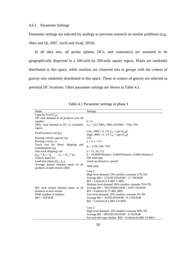
50

4.6.1 Parameter Settings

Parameter settings are selected by analogy to previous research on similar problems (e.g.,

Shen and Qi, 2007, Javid and Azad, 2010).

In all data sets, all points (plants, DCs, and customers) are assumed to be

geographically dispersed in a 500-mile by 500-mile square region. Plants are randomly

distributed in this space, while retailers are clustered into m groups with the centers of

gravity also randomly distributed in this space. These m centers of gravity are selected as

potential DC locations. Other parameter settings are shown in Table 4.1.

Table 4.1 Parameter settings in phase I

Name Settings Capacity level (Cjk) TD: total demand of all products over all retailers. TRDj: total demand in DC j’s reachable region.

k = 4 Cjk = {0.5 TRDj, TRDj, 05(TRDj + TD), TD}

Fixed location cost (fjk) Low: 2000 + 0. 1*[ Cjk + sqrt (Cjk)] High: 4000 + 0. 2*[ Cjk + sqrt (Cjk)]

Routing vehicle capacity (q) 150 Routing cost (a, c) a = 5, c = 0.1 Truck size for direct shipping and transshipment (ql)

ql = {150, 500, 750}

One truck shipping cost (apjl + bpjl * ql ajj’l + bjj’l * ql)

a = {5, 10, 12} b = {0.0006*distance, 0.0004*distance, 0.0003*distance}

Vehicle speed (s) 500 miles/day Lead time (days) (ltpj, ltjj’ ) round up (distance / speed) Average annual demand mean of all products at each retailer (MD)

3000 units

RD: total annual demand mean of all products at each retailer NOR: number of retailers MD = TD/NOR

Case 1: High level demand: 10% retailers consume 27% TD. Average RD = 27%TD/10%NOR = 2.7 TD/NOR RDi = Uniform (2.4 MD, 3 MD) Medium level demand: 80% retailers consume 70% TD. Average RD = 70%TD/80%NOR = 0.875 TD/NOR RDi = Uniform (0.75 MD, MD) Low level demand: 10% retailers consume 3% TD. Average RD = 3%TD/10%NOR = 0.3 TD/NOR RDi = Uniform (0.2 MD, 0.4 MD) Case 2: High level demand: 10% retailers consume 80% TD. Average RD = 80%TD/10%NOR = 8 TD/NOR For each this type retailer: RDi = Uniform (6 MD, 10 MD )

51

Name Settings Medium level demand: 10% retailers consume 10% TD. Average RD = 10%TD/10%NOR = TD/NOR RDi = Uniform (0.8 MD, 1.2 MD) Low level demand: 80% retailers consume 10% TD. Average RD = 10%TD/80%NOR = 0.125 TD/NOR RDi = Uniform (0.05 MD, 0.2 MD)

Annual demand mean of each product at each retailer (µpi) NOP: number of types of products PDi = RDi /NOP

High level demand product: 10% products consume 27% RD µpi = Uniform(2.4 PDi, 3 PDi) Medium level demand product: 80% products consume 70% RD µpi = Uniform(0.75 PDi, PDi) Low level demand product: 10% products consume 3% RD µpi = Uniform(0.2 PDi, 0.4 PDi)

Standard deviation of demand (σpi) µpi * Uniform(0, 0.1)

Annual unit holding cost (hpj)

Holding cost at DCs = Holding cost at retailers /2 Holding cost at retailers: Low level: $15/(year*unit) High level: $ 30/(year*unit)

Service level 97.5%: zα = 1.96 Available routing frequency {350, 175, 50, 25}, 1 year = 350 days Routing distance limit 500 miles

4.6.2 Lower Bound Generation

As mentioned earlier, the original model, even the modified model introduced in Section

4.3 with iteratively updating the safety stock coefficients, is quite difficult to solve in

medium and large instances. In order to provide an evaluation of the proposed heuristics,

another modified model will be introduced here.

The major complexity in the model comes from transshipments where product mix

exists. If the transshipment related component in the objective function (4-6) is ignored,

then the shipping and inventory cost is simplified from equation (4-24) to equation (4-25).

In addition, in the single PW case, if any DC is selected as a PW, the quantity shipped

between the plant and this DC is determined as the total demand. In this case equation

(4-25) can be rewritten as equation (4-26) by adding binary variable Wpj (1 if DC j is a

PW for facility p, 0 otherwise).

52

( )

( )

,

'

'' , ''

2 2' ' ', ' ' , '

, ' '

' , ''

= +

2 2

j pj pj pjj J p P j J

pj jpj p Ppj j jp P j J j j

pj j j

pj pi pjj i j j pi pj jii I j J j J j j i I

pjp P j pj j j pj j

j J j jpj jp P

SC h SS RI

QQA A

q q

z lt Y lt Y

h q q Q

Q

α σ σ

∈ ∈ ∈

∈

∈ ∈ ≠

∈ ∈ ∈ ≠ ∈

∈ ∈

∈ ≠∈

+ +

+

+ + +

∑ ∑∑

∑ ∑

∑ ∑ ∑

∑ ∑J∑

(4-24)

2', , '

+2

pj pjpj pj pj pi pjj ip P p P j J i I j J

pj

Q qA h z lt Y

q α σ∈ ∈ ∈ ∈ ∈

≥ +

∑ ∑ ∑ (4-25)

( )

2

, , '

,

2

, '

=2

Where min2

pi pj pji Ipj pj pj pi pjp P j J i I j J

pj

pj pjp P j J

pi pj li Ipj l L pjl pjl l pj pj pii I j J

l

h qA h z lt W

q

W

h qa b q h z lt

q

α

α

µσ

ω

µω σ

∈∈ ∈ ∈ ∈

∈ ∈

∈∈ ∈ ∈

+ + ⋅

=

= + + +

∑∑ ∑

∑∑ ∑

(4-26)

So the modified model without considering transshipment costs the objective function

becomes, in the single PW case, to minimize:

, pj pjp P j JFC IRC Wω

∈ ∈+ +∑ (4-27)

Subject to: Constraints (4-7) – (4-16) with PWp = 1. This makes the formulation an

integer programing model which can be solved by standard optimization software

directly in small-medium instances.

4.6.3 Results and Analysis

In this section, computational results are presented for 8 different data sets with each set

including 15 scenarios which sizes ranging from 20 to 200 retailers and 5 to 20 products.

53

Those 8 data sets differ in fixed location cost rate (low, high), demand rate (case 1, case 2)

and holding cost rate (low, high). Table 4.2 and 4.3 show the construction of all scenarios,

and Table 4.4 summarizes results from all experiments including objective value,

computational time, and the number of opened DCs under each scenario. All the time is

obtained on a Intel(R) Core(TM)2 T5550 at 1.83 GHz using Windows 7.

Table 4.2 Scenario construction in phase I: part A

Scenario Condition

1-15 Fixed cost = Low; Demand = Case1; Holding cost = High

16-30 Fixed cost = Low; Demand = Case1; Holding cost = Low

31-45 Fixed cost = Low; Demand = Case2; Holding cost = High

46-60 Fixed cost = Low; Demand = Case2; Holding cost = Low

61-75 Fixed cost = High; Demand = Case1; Holding cost = High

76-90 Fixed cost = High; Demand = Case1; Holding cost = Low

91-105 Fixed cost = High; Demand = Case2; Holding cost = High

106-120 Fixed cost = High; Demand = Case2; Holding cost = Low

Table 4.3 Scenario construction in phase I: part B

Scenario NOP NOR NODC

1 16 31 46 61 76 91 106 5 20 2

2 17 32 47 62 77 92 107 5 50 5

3 18 33 48 63 78 93 108 5 100 10

4 19 34 49 64 79 94 109 5 150 10

5 20 35 50 65 80 95 110 5 200 20

6 21 36 51 66 81 96 111 10 20 2

7 22 37 52 67 82 97 112 10 50 5

8 23 38 53 68 83 98 113 10 100 10

9 24 39 54 69 84 99 114 10 150 10

10 25 40 55 70 85 100 115 10 200 20

11 26 41 56 71 86 101 116 20 20 2

12 27 42 57 72 87 102 117 20 50 5

13 28 43 58 73 88 103 118 20 100 10

14 29 44 59 74 89 104 119 20 150 10

15 30 45 60 75 90 105 120 20 200 20

54

Table 4.4 Best solution scenarios and average GAP in phase I

TSSA IRC FC

Best Solution Scenarios 27 of 120 74 of 120 52 of 120

Average GAP 12.9% 1.2% 2.0%

In Table 4.3, NOP is the number of plants (different products), NOR is the number of

retailers and NODC is the number of potential DC locations. Five random instances were

generated for each experimental scenario. The three heuristics are then applied to each

scenario in Microsoft Visio Studio C++, and the result for each scenario is the average of

those five random instances. IBM ILOG CPLEX Optimization Studio is used to solve the

modified model and lower bound model. Only some small instances of the original model

can be solved in a reasonable time. Note that since the truck size is selected off-line, the

result is not guaranteed to be the true optimal solution. For the lower bound model, some

scenarios can be solved directly using CPLEX, otherwise current objective value and best

integer solution after running 1 hour is recorded. In addition, Table 4.5 records the

improvement using heuristics ((1 – Best heuristics solution/Original solution) × 100%)

and individual heuristic’s GAP ((Heuristic solution/Best heuristics solution - 1) × 100%).

Figure 4.5 illustrates objective values from five different solution methods (original

greedy solution, TSSA method, IRC heuristic, FC heuristic and lower bound solution).

It’s clearly shown that direct heuristics improve the original greedy solution significantly

and close to lower bound solution value. Since it is hard to tell the differences in small

instances, Figure 4.5 is transformed to Figure 4.6 by talking the log function over the

objective value.

55

Figure 4.5 Test result comparison between solving methods

Figure 4.6 Log transfermation of results

In addition, five figures are presented, each contains 24 cases covering the 8 scenarios

with 5, 10 and 20 plants respectively. The figures are separated by the number of retailers.

0

2

4

6

8

10

12

14

16

0 5 10 15 20 25 30 35 40 45 50 55 60 65 70 75 80 85 90 95 100105110115120

x 1

00

00

0

Original Solution TSSA Method IRC Heuristic FC Heuristic LowerBound Solution

4.5

4.7

4.9

5.1

5.3

5.5

5.7

5.9

6.1

6.3

0 5 10 15 20 25 30 35 40 45 50 55 60 65 70 75 80 85 90 95 100105110115120


56

For example, Figure 4.7 is the result for NOR = 20, NODC = 2, and there are in total 24

such cases as shown in bold in Table 4.3.

Figure 4.7 Results when NOR = 20, NODC = 2


3

4

5

6

7

8

9

10

0 5 10 15 20 25 30 35 40 45 50 55 60 65 70 75 80 85 90 95 100105110115120

x 1

00

00

Original solution TSSA Method IRC Heuristic FC Heuristic LowerBound Solution

7

9

11

13

15

17

19

21

23

25

0 5 10 15 20 25 30 35 40 45 50 55 60 65 70 75 80 85 90 95 100105110115120

x 1

00

00


57



1

2

3

4

5

6

7

0 5 10 15 20 25 30 35 40 45 50 55 60 65 70 75 80 85 90 95 100105110115120

x 1

00

00

0


2

3

4

5

6

7

8

9

0 5 10 15 20 25 30 35 40 45 50 55 60 65 70 75 80 85 90 95 100105110115120

x 1

00

00

0

Original Solution TSSA Method IRC Heristic FC Heuristic LowerBound Solution

58


From all the experiment running results, the following observations are obtained:

1. All instances are solved in a reasonable time by the heuristics, with the maximum

computation time of one hour. Note that even small instances (e.g., scenario 3) could

not be solved optimally by CPLEX software after two hours of computation.

2. Heuristics work well in terms of objective values compared to the original greedy

solution and the lower bound. The original solution’s objective value is reduced by

26.9% on average, and the improvement is greater under large instances. The best

heuristic’s solution is only 11.1% higher than the lower bound solution and 5.7%

higher than the integer solution of CPLEX after one hour running, note that the lower

bound values do not include transshipment consideration and large instances do not

converge completely in CPLEX (a Gap between current solution and the best integer

solution exists).

2

4

6

8

10

12

14

16

0 5 10 15 20 25 30 35 40 45 50 55 60 65 70 75 80 85 90 95 100105110115120

x 1

00

00

0

Original Solution TSSA Method IRC Heristic FC Heristic LowerBound Solution

3. Results from IRC and FC heuristics

in large instances. This is because TSSA method is embedded in IRC and FC

heuristics as a post-improvement step, indicat

point.

4. Differences among different s

instances (Figure 4.7 through Figure 4.11). In small intances, even

heuristic could find a good/optimal solution in a reasonable time.

5. IRC heuristic performs the best in both the number of best solution scenarios an

average GAP as shown in Table

in the system is IRC and the

smallest total IRC. Figure

experiments.

0%

10%

20%

30%

40%

50%

60%

70%

80%

90%

100%

FCRate = Low; HCRate = Low

FCRate = Low; HCRate = High

21.9%

57.4%

6.9%

13.7%

59

Results from IRC and FC heuristics are better than simple TSSA method, especially


improvement step, indicating the importance of a good starting

Differences among different solution methods become more obviou

instances (Figure 4.7 through Figure 4.11). In small intances, even

heuristic could find a good/optimal solution in a reasonable time.

IRC heuristic performs the best in both the number of best solution scenarios an

as shown in Table 4.4. This may be because the largest cost component

and the IRC heuristic starts with a feasible solution with the

Figure 4.12 shows the cost components among all

Figure 4.12 Cost components

FCRate = Low; HCRate = High

FCRate = High; HCRate = Low

FCRate = High; HCRate = High

21.9% 16.2% 35.9% 27.9%

57.4% 63.4% 47.1% 54.3%

6.9% 7.4% 5.4% 6.9%

13.7% 12.9% 11.7% 10.9%

are better than simple TSSA method, especially


the importance of a good starting

ous in large

instances (Figure 4.7 through Figure 4.11). In small intances, even the simple

IRC heuristic performs the best in both the number of best solution scenarios and the

be because the largest cost component

IRC heuristic starts with a feasible solution with the

shows the cost components among all running

27.9%

54.3%

6.9%

10.9%

SC

IC

IRC

FC

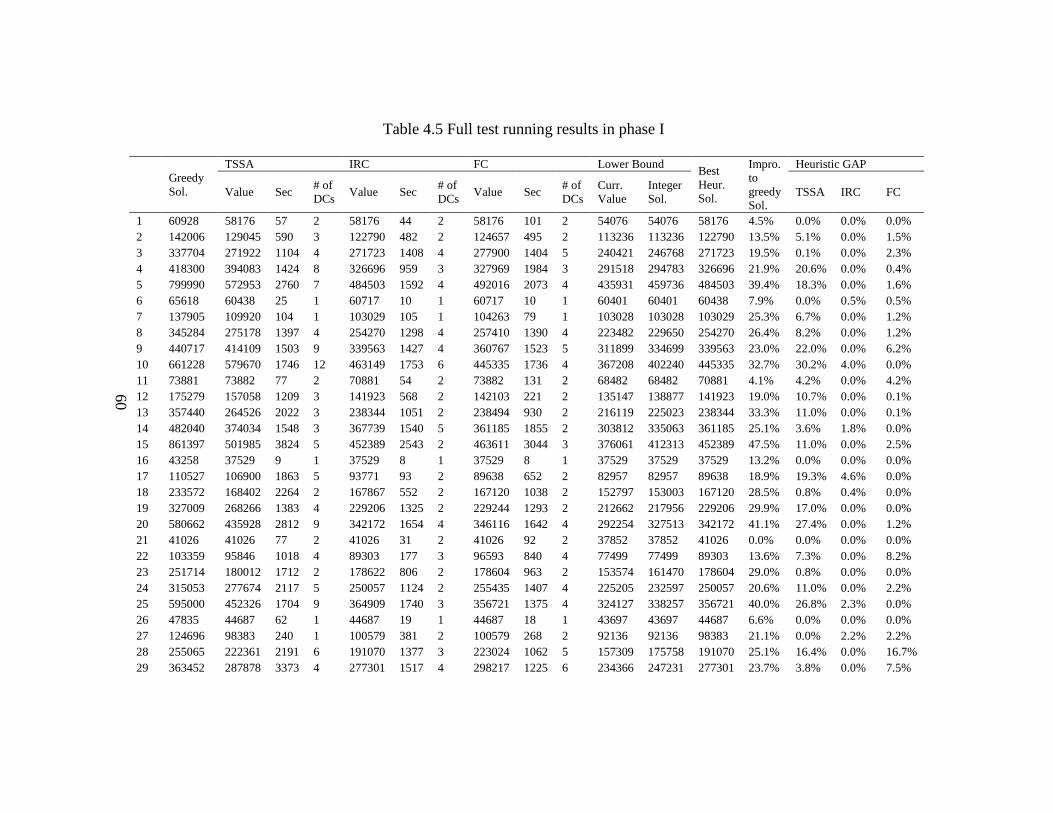
60

Table 4.5 Full test running results in phase I

Greedy Sol.

TSSA IRC FC Lower Bound Best Heur. Sol.

Impro. to greedy Sol.

Heuristic GAP

Value Sec # of DCs

Value Sec # of DCs

Value Sec # of DCs

Curr. Value

Integer Sol.

TSSA IRC FC

1 60928 58176 57 2 58176 44 2 58176 101 2 54076 54076 58176 4.5% 0.0% 0.0% 0.0% 2 142006 129045 590 3 122790 482 2 124657 495 2 113236 113236 122790 13.5% 5.1% 0.0% 1.5% 3 337704 271922 1104 4 271723 1408 4 277900 1404 5 240421 246768 271723 19.5% 0.1% 0.0% 2.3% 4 418300 394083 1424 8 326696 959 3 327969 1984 3 291518 294783 326696 21.9% 20.6% 0.0% 0.4% 5 799990 572953 2760 7 484503 1592 4 492016 2073 4 435931 459736 484503 39.4% 18.3% 0.0% 1.6% 6 65618 60438 25 1 60717 10 1 60717 10 1 60401 60401 60438 7.9% 0.0% 0.5% 0.5% 7 137905 109920 104 1 103029 105 1 104263 79 1 103028 103028 103029 25.3% 6.7% 0.0% 1.2% 8 345284 275178 1397 4 254270 1298 4 257410 1390 4 223482 229650 254270 26.4% 8.2% 0.0% 1.2% 9 440717 414109 1503 9 339563 1427 4 360767 1523 5 311899 334699 339563 23.0% 22.0% 0.0% 6.2% 10 661228 579670 1746 12 463149 1753 6 445335 1736 4 367208 402240 445335 32.7% 30.2% 4.0% 0.0% 11 73881 73882 77 2 70881 54 2 73882 131 2 68482 68482 70881 4.1% 4.2% 0.0% 4.2% 12 175279 157058 1209 3 141923 568 2 142103 221 2 135147 138877 141923 19.0% 10.7% 0.0% 0.1% 13 357440 264526 2022 3 238344 1051 2 238494 930 2 216119 225023 238344 33.3% 11.0% 0.0% 0.1% 14 482040 374034 1548 3 367739 1540 5 361185 1855 2 303812 335063 361185 25.1% 3.6% 1.8% 0.0% 15 861397 501985 3824 5 452389 2543 2 463611 3044 3 376061 412313 452389 47.5% 11.0% 0.0% 2.5% 16 43258 37529 9 1 37529 8 1 37529 8 1 37529 37529 37529 13.2% 0.0% 0.0% 0.0% 17 110527 106900 1863 5 93771 93 2 89638 652 2 82957 82957 89638 18.9% 19.3% 4.6% 0.0% 18 233572 168402 2264 2 167867 552 2 167120 1038 2 152797 153003 167120 28.5% 0.8% 0.4% 0.0% 19 327009 268266 1383 4 229206 1325 2 229244 1293 2 212662 217956 229206 29.9% 17.0% 0.0% 0.0% 20 580662 435928 2812 9 342172 1654 4 346116 1642 4 292254 327513 342172 41.1% 27.4% 0.0% 1.2% 21 41026 41026 77 2 41026 31 2 41026 92 2 37852 37852 41026 0.0% 0.0% 0.0% 0.0% 22 103359 95846 1018 4 89303 177 3 96593 840 4 77499 77499 89303 13.6% 7.3% 0.0% 8.2% 23 251714 180012 1712 2 178622 806 2 178604 963 2 153574 161470 178604 29.0% 0.8% 0.0% 0.0% 24 315053 277674 2117 5 250057 1124 2 255435 1407 4 225205 232597 250057 20.6% 11.0% 0.0% 2.2% 25 595000 452326 1704 9 364909 1740 3 356721 1375 4 324127 338257 356721 40.0% 26.8% 2.3% 0.0% 26 47835 44687 62 1 44687 19 1 44687 18 1 43697 43697 44687 6.6% 0.0% 0.0% 0.0% 27 124696 98383 240 1 100579 381 2 100579 268 2 92136 92136 98383 21.1% 0.0% 2.2% 2.2% 28 255065 222361 2191 6 191070 1377 3 223024 1062 5 157309 175758 191070 25.1% 16.4% 0.0% 16.7% 29 363452 287878 3373 4 277301 1517 4 298217 1225 6 234366 247231 277301 23.7% 3.8% 0.0% 7.5%

61

Greedy Sol.



Heuristic GAP

Value Sec # of DCs

Value Sec # of DCs

Value Sec # of DCs

Curr. Value

Integer Sol.

TSSA IRC FC

30 696137 477341 1504 9 363754 1449 3 365486 1372 3 289488 329951 363754 47.7% 31.2% 0.0% 0.5% 31 66558 64577 28 2 65313 32 2 65313 35 2 60792 60792 64577 3.0% 0.0% 1.1% 1.1% 32 159410 141331 1344 2 138424 75 1 138424 119 1 132915 132915 138424 13.2% 2.1% 0.0% 0.0% 33 446165 416010 1365 7 346922 1262 4 343589 750 3 304534 305096 343589 23.0% 21.1% 1.0% 0.0% 34 529884 405186 1725 2 389906 1187 2 380801 1380 2 348789 369088 380801 28.1% 6.4% 2.4% 0.0% 35 894131 639446 2069 8 545477 1635 4 554409 1155 2 474156 503618 545477 39.0% 17.2% 0.0% 1.6% 36 74593 68898 25 1 69096 11 1 69096 13 1 68600 68600 68898 7.6% 0.0% 0.3% 0.3% 37 198341 172594 959 2 176813 575 2 176487 329 2 154638 154638 172594 13.0% 0.0% 2.4% 2.3% 38 433334 375889 1709 4 344253 2182 3 349761 1285 4 305400 308485 344253 20.6% 9.2% 0.0% 1.6% 39 551753 444324 2599 3 412235 1381 2 406041 1305 2 377265 378713 406041 26.4% 9.4% 1.5% 0.0% 40 1001097 568855 2775 3 569713 1748 5 582380 1356 4 459516 517488 568855 43.2% 0.0% 0.2% 2.4% 41 70061 68748 55 1 68748 13 1 68748 15 1 65854 65854 68748 1.9% 0.0% 0.0% 0.0% 42 176209 163091 672 2 148289 539 2 154290 551 2 140476 140476 148289 15.8% 10.0% 0.0% 4.0% 43 511315 424480 1762 6 373717 1325 3 362337 1421 3 312129 329219 362337 29.1% 17.2% 3.1% 0.0% 44 595933 505879 2350 5 460701 1464 3 469338 1376 3 391592 417683 460701 22.7% 9.8% 0.0% 1.9% 45 1029142 711828 3600 7 637322 1134 3 648089 1472 4 506430 587654 637322 38.1% 11.7% 0.0% 1.7% 46 55017 49203 19 1 49203 11 1 49203 11 1 49203 49203 49203 10.6% 0.0% 0.0% 0.0% 47 151329 141750 796 3 140380 152 3 142111 267 3 122096 122096 140380 7.2% 1.0% 0.0% 1.2% 48 314144 273545 1477 6 231574 1358 3 249097 1732 3 205091 212383 231574 26.3% 18.1% 0.0% 7.6% 49 477297 374641 1756 4 372730 980 3 349354 1287 2 304157 320974 349354 26.8% 7.2% 6.7% 0.0% 50 784966 533026 1667 7 409663 1651 3 423902 1647 3 358988 390211 409663 47.8% 30.1% 0.0% 3.5% 51 59667 52792 24 1 52792 14 1 52792 15 1 52792 52792 52792 11.5% 0.0% 0.0% 0.0% 52 165152 148894 570 3 135331 177 2 141785 433 2 123936 123936 135331 18.1% 10.0% 0.0% 4.8% 53 285721 214268 1702 2 217315 1303 2 210704 1273 2 195732 200555 210704 25.0% 1.7% 3.1% 0.0% 54 451527 398527 2115 6 345879 1436 3 340996 1311 2 302856 313759 340996 24.5% 16.9% 1.4% 0.0% 55 821873 645541 2117 12 465626 2195 4 455408 2718 3 376349 444348 455408 44.6% 41.8% 2.2% 0.0% 56 49168 44449 24 1 44449 19 1 44449 23 1 44449 44449 44449 9.6% 0.0% 0.0% 0.0% 57 141823 136109 2694 4 123224 709 2 128525 387 2 111402 111402 123224 13.1% 10.5% 0.0% 4.3% 58 316108 297240 1407 8 236447 1419 3 236809 1388 3 193303 208582 236447 25.2% 25.7% 0.0% 0.2% 59 476277 422932 1545 6 361695 1531 3 389890 1518 4 315353 331703 361695 24.1% 16.9% 0.0% 7.8% 60 869445 566097 2663 7 510900 1480 4 519367 1202 3 394021 491387 510900 41.2% 10.8% 0.0% 1.7%

62

Greedy Sol.



Heuristic GAP

Value Sec # of DCs

Value Sec # of DCs

Value Sec # of DCs

Curr. Value

Integer Sol.

TSSA IRC FC

61 68884 65898 42 2 65359 48 2 65359 77 2 62230 62230 65359 5.1% 0.8% 0.0% 0.0% 62 176373 150616 171 2 157944 214 3 157706 1121 3 138503 138503 150616 14.6% 0.0% 4.9% 4.7% 63 380172 341329 1151 6 279400 1061 4 274207 1308 3 250760 252766 274207 27.9% 24.5% 1.9% 0.0% 64 556114 494886 1432 7 413921 1298 3 426706 1041 4 364094 374002 413921 25.6% 19.6% 0.0% 3.1% 65 1075650 715383 2131 9 561637 1216 4 559222 1160 3 504923 542152 559222 48.0% 27.9% 0.4% 0.0% 66 59810 52715 14 1 52715 9 1 52715 12 1 52715 52715 52715 11.9% 0.0% 0.0% 0.0% 67 190322 158039 1958 3 136632 280 2 152496 804 2 131338 131338 136632 28.2% 15.7% 0.0% 11.6% 68 430563 384282 1400 8 263430 1357 2 278752 953 3 237787 245432 263430 38.8% 45.9% 0.0% 5.8% 69 549299 456546 3600 6 392281 1072 2 397130 1420 3 346869 375594 392281 28.6% 16.4% 0.0% 1.2% 70 1157796 647292 2138 6 527163 1850 4 521174 2047 3 464898 500148 521174 55.0% 24.2% 1.1% 0.0% 71 79361 67570 15 1 67570 8 1 67570 8 1 67570 67570 67570 14.9% 0.0% 0.0% 0.0% 72 183478 162198 1953 3 147635 442 2 151387 562 2 138159 138159 147635 19.5% 9.9% 0.0% 2.5% 73 439712 322804 1727 5 282332 2067 3 307578 1395 4 241937 264686 282332 35.8% 14.3% 0.0% 8.9% 74 566400 456581 1541 4 399406 1562 2 382505 1430 2 356532 370689 382505 32.5% 19.4% 4.4% 0.0% 75 1101735 567338 2357 4 544567 1533 4 552659 1860 5 438662 525805 544567 50.6% 4.2% 0.0% 1.5% 76 50857 50857 73 2 49529 33 2 50857 21 2 47073 47073 49529 2.6% 2.7% 0.0% 2.7% 77 133244 105986 973 3 97220 491 2 102459 269 2 94362 94362 97220 27.0% 9.0% 0.0% 5.4% 78 325846 196153 1317 2 175547 904 2 175668 1173 2 169555 169555 175547 46.1% 11.7% 0.0% 0.1% 79 420871 357470 1408 7 300592 1393 3 314397 1399 3 270301 273611 300592 28.6% 18.9% 0.0% 4.6% 80 883370 577745 2074 9 380826 1618 3 391847 1262 3 337052 402026 380826 56.9% 51.7% 0.0% 2.9% 81 53905 52963 54 2 52568 194 2 51981 299 2 48543 48543 51981 3.6% 1.9% 1.1% 0.0% 82 145144 111076 1246 2 111693 767 2 111846 184 2 102494 102494 111076 23.5% 0.0% 0.6% 0.7% 83 344524 224603 1689 3 229454 786 3 230265 949 3 190260 205813 224603 34.8% 0.0% 2.2% 2.5% 84 452943 382455 1486 7 341346 1126 4 367218 2430 6 277406 310517 341346 24.6% 12.0% 0.0% 7.6% 85 858688 401240 2978 4 365487 2159 3 369824 1753 3 315742 504757 365487 57.4% 9.8% 0.0% 1.2% 86 58814 57956 188 2 58340 66 2 57742 77 2 53173 53173 57742 1.8% 0.4% 1.0% 0.0% 87 146010 126613 2024 3 114123 929 2 114306 632 2 105516 105516 114123 21.8% 10.9% 0.0% 0.2% 88 354070 300222 1724 6 245455 1460 3 237488 1046 3 202558 216255 237488 32.9% 26.4% 3.4% 0.0% 89 427952 362378 3119 6 315837 1245 3 288894 1103 2 253679 291011 288894 32.5% 25.4% 9.3% 0.0% 90 946959 510910 2657 6 420331 1870 3 394520 1222 2 324934 380298 394520 58.3% 29.5% 6.5% 0.0% 91 90095 86007 30 2 88531 16 2 88927 24 2 81467 81467 86007 4.5% 0.0% 2.9% 3.4%

63

Greedy Sol.



Heuristic GAP

Value Sec # of DCs

Value Sec # of DCs

Value Sec # of DCs

Curr. Value

Integer Sol.

TSSA IRC FC

92 194878 166118 1188 3 152264 1968 2 150302 1320 2 143792 143792 150302 22.9% 10.5% 1.3% 0.0% 93 565169 487431 3600 8 403239 923 3 431002 1366 5 344913 349693 403239 28.7% 20.9% 0.0% 6.9% 94 687053 538956 1415 5 486360 1067 3 435454 1286 2 427661 428235 435454 36.6% 23.8% 11.7% 0.0% 95 1381632 987433 2421 11 596740 1552 2 597183 1544 2 570956 591129 596740 56.8% 65.5% 0.0% 0.1% 96 84364 76619 10 1 76619 8 1 76619 8 1 76619 76619 76619 9.2% 0.0% 0.0% 0.0% 97 195399 168463 668 3 170204 541 3 164652 851 3 147878 147878 164652 15.7% 2.3% 3.4% 0.0% 98 539073 439129 1384 6 358524 940 2 355543 940 2 336592 337885 355543 34.0% 23.5% 0.8% 0.0% 99 836530 659383 1803 6 605684 1411 4 605422 1382 4 510174 532667 605422 27.6% 8.9% 0.0% 0.0% 100 1315789 739312 2138 6 629805 1747 4 598945 2949 4 504104 601443 598945 54.5% 23.4% 5.2% 0.0% 101 88119 80613 15 1 80613 9 1 80613 12 1 80047 80047 80613 8.5% 0.0% 0.0% 0.0% 102 233553 196393 1685 3 181776 693 2 185652 472 2 166329 166329 181776 22.2% 8.0% 0.0% 2.1% 103 631148 421742 3499 3 400342 1233 2 401952 1250 2 357133 379786 400342 36.6% 5.3% 0.0% 0.4% 104 824451 689145 1533 6 622704 1522 6 556633 1031 2 482332 522064 556633 32.5% 23.8% 11.9% 0.0% 105 1302067 769948 1778 9 579574 1371 3 631934 1837 5 472642 545655 579574 55.5% 32.8% 0.0% 9.0% 106 69782 54977 9 1 54977 9 1 54977 8 1 54977 54977 54977 21.2% 0.0% 0.0% 0.0% 107 189229 150383 287 2 148684 264 2 137733 651 2 121184 121184 137733 27.2% 9.2% 8.0% 0.0% 108 455272 332581 1757 5 266417 1353 3 255938 1285 2 239472 246359 255938 43.8% 29.9% 4.1% 0.0% 109 778168 620148 1444 6 512949 1092 3 513892 1424 4 432317 449721 512949 34.1% 20.9% 0.0% 0.2% 110 1202676 831707 3600 11 559753 1605 3 554113 1274 3 483731 601756 554113 53.9% 50.1% 1.0% 0.0% 111 88432 72994 11 1 72994 8 1 72994 15 1 72994 72994 72994 17.5% 0.0% 0.0% 0.0% 112 155882 144041 1052 4 122214 603 2 122214 542 2 110864 110864 122214 21.6% 17.9% 0.0% 0.0% 113 375032 268071 1418 4 239700 1365 3 217811 902 2 203755 220346 217811 41.9% 23.1% 10.0% 0.0% 114 607656 550787 1502 8 435270 1497 3 455483 1830 4 424069 436657 435270 28.4% 26.5% 0.0% 4.6% 115 1506312 832701 3544 7 590362 1661 3 591865 2093 3 505267 790495 590362 60.8% 41.0% 0.0% 0.3% 116 74736 63866 13 1 63866 9 1 63866 13 1 63866 63866 63866 14.5% 0.0% 0.0% 0.0% 117 196019 169072 1179 3 150043 1328 2 163246 1204 2 140460 140832 150043 23.5% 12.7% 0.0% 8.8% 118 447562 296019 3809 3 302342 1056 3 316288 1450 4 257485 302548 296019 33.9% 0.0% 2.1% 6.8% 119 801576 504925 1432 2 550683 1146 3 538847 1542 3 433571 513144 504925 37.0% 0.0% 9.1% 6.7% 120 1277470 714982 3834 7 637893 1349 4 700747 2226 6 496549 654710 637893 50.1% 12.1% 0.0% 9.9%

64

5. PHASE II: INVENTORY ROUTING PROBLEM

The Inventory Routing Problem (IRP) is the final state distribution problem of the

proposed integrated supply chain design problem. From the previous phase, DCs’

locations and retailers’ assignments are determined. In this phase, the IRP is considered

separately for each opened DC and its assigned retailers. The goal is to decide routing

tours to each retailer and routing frequencies of each tour so that the total routing and

inventory cost is minimized over an infinite planning horizon.


A one-to-many IRP is considered in this phase for each opened DC and its assigned

retailers. The DC owns multiple homogenous capacitated vehicles, and each routing tour

should start and end at the DC. While demand is random, I seek to form standard tours

and frequencies. Individual orders will vary based on recent usage and vehicle capacity

will be considered to ensure a high probability of being able to meet demand on each

route trip. Routing frequencies are assumed to fall in a discrete set such as daily, every

other day, weekly and biweekly.

In this problem, the total cost is a summation of routing cost over each trip and

inventory cost at each retailer for a specified length of time. In this dissertation, I

consider the static problem and use average cost per period. Routing cost of one trip

contains a predetermined fixed cost and a variable cost depending on total distance of this

trip. Inventory at each retailer contains both cycle inventory and safety stock. Lead time

is assumed to be a function of routing frequency and distance.

65

For each DC j and all retailers i assigned to it, let R be the set of retailers and

0 { }R R DC j= U . Other parameters and variables are the same as defined in Section 3.2.

To be convenient, some of the definitions are rewritten here as follows.

P set of plants

R set of retailers assigned to the specific DC j

N set of available routing frequencies

V set of tours

zα left α-percentile of standard normal random variable Z

Miv Auxiliary variable defined for retailer i for subtour elimination in route of

vehicle v

µpi mean of annual demand of product p at retailer i

σ2pi variance of annual demand of product p at retailer i

ltst lead time from node s to node t

hps annual holding cost of product p per unit at point storing point s

D routing distance limit per trip

q routing vehicle’s capacity

dst distance from node s to node t

s speed of the default vehicle

a fixed cost of using one routing vehicle at DCs

c unit routing delivery cost per mile

fn routing frequency at level n

66

Xstv 1 if s immediate precedes t in route v, 0 otherwise

Rvi 1 if use route v to supply demand at retailer i, 0 otherwise

Zvn 1 if route v has routing frequency at level n, 0 otherwise

v n vnn Nf Zγ

∈=∑ the number of trips for route v in one year

,v st stvs t I Jd d X

∈=∑ U

the distance of route v

1 v viv Vi

v viv V

d Rlt

R sγ∈

∈

= +∑∑

the lead time for the retailer i. Lead time is a

function of routing route frequency (first component) and route distance (second

component)

Mixed Integer Programming Model

The IRP problem of interest can then be formulated as follows:

Minimize ( )0.5 pip P

v v pi pi rv V i R p P v Vvi vv V

a cd h z ltR α

µγ σ

γ∈

∈ ∈ ∈ ∈∈

+ + +

∑∑ ∑ ∑ ∑∑

(5-1)

Subject to:

1 viv VR i R

∈= ∀ ∈∑ (5-2)

, pi vip P i R

v

Rq v V

µ

γ∈ ∈ ≤ ∀ ∈

∑ (5-3)

vd D v V≤ ∀ ∈ (5-4)

( )| | | | 1 , ,sv tv stvM M R X R s t R v V− + × ≤ − ∀ ∈ ∈ (5-5)

0 00 ,stv tsvs R s R

X X t R v V∈ ∈

= ∀ ∈ ∈∑ ∑ (5-6)

67

( )0

0 ,1 iv stvi R s t R

R X X v V∈ ∈

+ ≥ ∀ ∈∑ ∑ (5-7)

0 ,itv vit R

X R i R v V∈

= ∀ ∈ ∈∑ (5-8)

1 vnn NZ v V

∈= ∀ ∈∑ (5-9)

0, , {0,1} , , , ,vi stv vnR X Z i R s t R v V n N∈ ∀ ∈ ∈ ∈ ∈ (5-10)

0 ,ivM i I v V≥ ∀ ∈ ∈ (5-11)

The objective function (5-1) has two components: routing cost and inventory cost.

Inventory cost includes both cycle inventory to meet foreseeable demand and safety stock

to overcome uncertain demand. Safety stock must cover demand uncertainty risk during

the replenishment lead time from placement of an order to receipt of the following order.

Equation (5-2) makes sure that each retailer is placed on exactly one vehicle route.

Inequalities (5-3) and (5-4) are vehicle capacity and distance limitation constraints for

each route. The left hand side of constraint (5-3) accumulates total expected demand for

all retailers on a route per trip. This must not exceed truck capacity. The right hand side

truck capacity can be adjusted to provide safety capacity if desired as actual delivery

amounts will vary dynamically with random demand. Constraint (5-5) eliminates subtour

which guarantees each route must contain a DC and at least one customer. Equation (5-6)

is flow conservation constraint that ensures routes are continuous and connected.

Constraint (5-7) implies that each effective route starts at a DC. ,v st stvs t I J

d d X∈

=∑ Uas

formulated in Section 3.2. Constraint (5-8) links the retailer-route allocation and the

68

routing components. Equation (5-9) is route frequency constraint. Constraints (5-10) and

(5-11) are integrality and non-negativity restrictions on the decision variables.

5.2 Problem Characteristics

Several problem characteristics are provided to facilitate solution generation.

5.2.1 Optimal Delivery Frequency

If a routing tour is decided, then retailers in this route and the routing cost per trip in this

route are known. To decide the optimal routing frequency is to Minimize:

0.5( )

v

prp Pv v r pr rr S p P

v

a cd h z lt v Vα

µγ σ

γ∈

∈ ∈

+ + + ∀ ∈

∑∑ ∑ (5-12)

subject to the vehicle capacity constraints, where Sv is the set of retailers serviced by this

route v. As a discrete variable having relatively few available values, you can simply try

each value and use the one minimizing the total cost. The nonlinearity of the objective

makes it difficult to obtain a closed form optimality expression, but the first and second

order derivatives are provided in the Appendix A for nonlinear search techniques.

In some cases, the optimal delivery frequency may cause a retailer to receive items at

a frequency other than their natural frequency (The optimal routing frequency for each

retailer under an individual tour is called the natural frequency for this retailer).

Figure 5.1 Two retailers: natural frequency example

DC r2

r1

10 mile

100 mile

100 mile

69

For example: Consider two retailers (r1, r2) which are close together, they are both

100 miles from their assigned DC and only 10 miles in between (as shown in Figure 5.1).

The total annual demand mean is µ1 = 1500, µ2 = 20000 and standard deviation is σ1 = 5,

σ2 = 50. Other parameter settings are shown in Table 5.1.

Table 5.1 Parameter settings for the natural frequency example

Name Notation Value

Vehicle capacity C 150

Fixed cost of each vehicle a 5

Variable routing cost c 0.1

Distance limit D 500

Individual route distance d1, d2 200

Joint route distance d12 210

Speed s 175000

Holding cost hr 10

Service level Z 1.96

To calculate the natural frequency for each retailer, select the optimal frequency from

available frequency set {350, 175, 50, 25} (Table 5.2). The optimal routing frequency

for joint tour is shown in Table 5.3.

Table 5.2 Natural frequency calculation for the natural frequency example

r1 r2

Frequency

Annual vehicle capacity

Annual routing cost

Lead time

Annual Holding cost

Total Cost

Annual Holding

cost Total Cost

350 52500 8750 0.0040 27.6 8777.6 347.7 9097.7

175 26250 4375 0.0069 51.0 4426.0 652.6 5027.6

50 7500 1250 0.0211 164.2 1414.2

25 3750 625 0.0411 319.9 944.9

Total Cost 5972.5

As shown in Table 5.2, the natural frequency for r1 is 25/year and for r2 is 175/year.

Notice that frequency {50, 25} is not available for r2 because of the vehicle capacity.

70

Total cost for both routes are $5972.5/year. However, if you combine the tours and use

only one route to sever both retailers, then the joint optimal frequency is 175/year with

total cost $5253.9. In this case, the optimal delivery frequency causes r2 to receive items

at a frequency other than its natural frequency.

Table 5.3 Joint tour optimal frequency calculation for the natural frequency example

Frequency Annual vehicle capacity Annual routing cost Lead time Annual Holding cost Total Cost

350 52500 9100 0.0041 375.8 9475.8

175 26250 4550 0.0069 703.9 5253.9

5.2.2 Upper/Lower Bounds for the Number of Tours

In this research, the optimal number of tours needed is not known. If using full-truck-load

to delivery products as often as possible (at the maximum allowed frequency,maxγ ), a

lower bound is generated asmax

r rLBV

C

µγ∑

= .

And if using one individual route for each retailer, then an upper bound is generated:

V UB = N. This upper bound is used later on in genetic algorithm to create chromosomes.

5.2.3 Upper/Lower Bounds for the Objective Values

The major benefit of routing comes from reduction in delivery cost. If there are no

distance/capacity limitations, nearest neighbors will be merged into one tour. In an ideal

case, delivery distance to one retailer is 1 + 1/ (N+1) times the distance between nearest

neighbors, where N is the total number of retailers. The smallest total number of trips

required is total demand for the period over all retailers divided by truck capacity. Let

71

IRC be total inventory routing cost, so a lower bound for the objective value is generated

as:

,

11

1

11

1 12

r r

prr R p PLB rr R

prp Pr prp P

r r

c dN

IRC a dC N

h zpα

γ

µµ

σγ γ

∈ ∈

∈∈

∈

+ + = + + + + + +

∑∑ ∑

∑ (5-13)

where dr is distance to its nearest neighbor for each retailer. The value of second part can

be found using methods introduced in the previous section.

The above lower bound is very tight, so an estimation of total cost is also generated

by considering delivery distance to each retailer as D / n, where D is the distance limit

and n is the average number of retailers in one route. This estimation formula is not a

lower bound, and is only used to estimate the possible optimal total routing cost.

1

2

prp Pe r r prr R p P

r r

a cD DIRC h z

n npα

µγ σ

γ γ∈

∈ ∈

+ = + + +

∑∑ ∑ (5-14)

Any feasible solution is an upper bound, a simple solution is using all direct-shipping.

In this case, each retailer has one individual route, and the frequency is selected to

minimize this individual tour.

5.3 Solution Methods

This proposed IRP belongs to the class of NP-hard problems as an extension of VRP to

include inventory concerns. The VRP in general is NP-hard as it lies at the intersection of

these two NP-hard problems: Traveling Salesman Problem and Bin Packing Problem. In

72

this section, several heuristics are developed to solve this IRP problem for medium and

large instances. The basic idea is to generate fixed partitions of retailers and use one

vehicle to serve one group of retailers. After a routing tour is determined within a group

of retailers, routing frequencies are selected from the available frequency set.

5.3.1 Modified Sweep Method (MS)

Evidence indicates that the sweep method for routing vehicles is computationally

efficient and produces an average gap from optimality of about 10 percent (Ballou, 2003).

This gap may be acceptable where results must be obtained in short order and good

solutions are needed as opposed to optimal ones.

The simple sweep method is modified by considering specific characteristics in this

problem: optimize routing tour after inserting each new retailer, optimize routing

frequency within the route, start from each retailer and sweep both clockwise and

counterclockwise. The procedure of the modified sweep method is as follows:

Figure 5.2 Sweep result example

5

4

DC

1

23

6

7

8

9

10

11

12

73

Procedure

1. Locate the DC and all retailers on a map or grid by polar coordinates with the center

at the DC.

2. Starting at any angle from the DC, and then rotate the line clockwise until it intersects

one retailer. For the first retailer the line intersects, build one individual route for this

retailer (retailer 1 in Figure 5.2).

3. Continue to rotate the line until next retailer is reached, insert new retailer in current

route using nearest insertion method and try to improve the new route by 2-opt

method. After including new retailer and deciding new optimal route in current route,

check all constraints and recalculate the optimal routing frequency and total cost.

4. If adding the new retailer to current route can reduce total cost and all constraints are

met, add this retailer to the current route; otherwise, create a new route starting at the

new retailer.

5. Continue until all retailers are assigned.

In step 4, after checking all constraints if adding the next retailer, two cases are

compared to finally decide whether to add this new retailer or not: one is to add this new

retailer resulting in one longer route, the other is the previous route and a new individual

route for this new retailer. Let:

RC routing cost per trip

IC inventory cost

IRC total inventory routing cost

γ optimal routing frequency

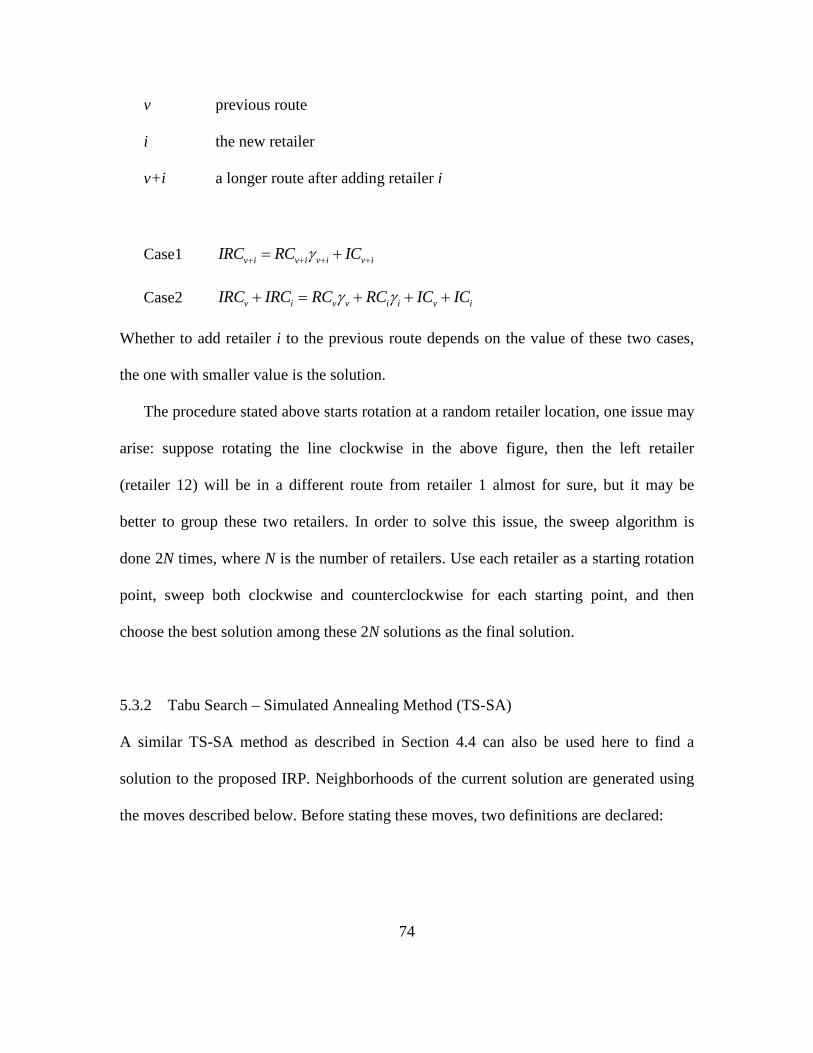
74

v previous route

i the new retailer

v+i a longer route after adding retailer i

Case1 v i v i v i v iIRC RC ICγ+ + + += +

Case2 v i v v i i v iIRC IRC RC RC IC ICγ γ+ = + + +

Whether to add retailer i to the previous route depends on the value of these two cases,

the one with smaller value is the solution.

The procedure stated above starts rotation at a random retailer location, one issue may

arise: suppose rotating the line clockwise in the above figure, then the left retailer

(retailer 12) will be in a different route from retailer 1 almost for sure, but it may be

better to group these two retailers. In order to solve this issue, the sweep algorithm is

done 2N times, where N is the number of retailers. Use each retailer as a starting rotation

point, sweep both clockwise and counterclockwise for each starting point, and then

choose the best solution among these 2N solutions as the final solution.

5.3.2 Tabu Search – Simulated Annealing Method (TS-SA)

A similar TS-SA method as described in Section 4.4 can also be used here to find a

solution to the proposed IRP. Neighborhoods of the current solution are generated using

the moves described below. Before stating these moves, two definitions are declared:

75

Distance between two routes: For all pairs of retailers in two different routes, the

smallest possible distance between two retailers is called the distance between these two

routes. Let Sk be the set of retailers included in route k; Dij be the distance between

retailer i and j, and DRmn be the distance between route m and n, then:

argmin{ } , mn ij m nDR D i S j S= ∈ ∈

Adjacent route: Two routes are called adjacent if the distance between these two

routes is the smallest compared to all other routes for at least one of the two routes.

Alternatively, define routes as adjacent if the distance is (or within some predetermined

value).

Move 1: Select two retailers in one route and then exchange their delivery order.

Move 2: Select two retailers from two adjacent routes and then exchange them.

Move 3: Select one retailer randomly and insert it to an adjacent route.

Move 4: Select one retailer randomly and then open a new individual route for it.

5.3.3 Integrated Local Search Method (ILS)

A distinction of this research is to simultaneously consider routing tour and routing

frequency over an infinite planning horizon while traditional routing solution methods

usually only focus on routing tour. In order to capture routing frequency, this integrated

local search method is proposed here.

The basic idea is to generate an initial solution where each retailer is serviced by one

individual tour, and then try to merge retailers into one route. The optimal routing

frequency for each retailer under an individual tour is called the natural frequency for this

76

retailer. This heuristic is also suitable if natural frequency is given in reality, for example,

some retailers receive orders daily/weekly.

When calculating the natural frequency, routing cost per trip is calculated as one fixed

vehicle cost plus variable cost from DC to the retailer. This is considering the

performance of one retailer in a joint routing tour with multi-retailers. The routing cost

for one retailer in such a tour is only part of one fixed cost and some inserted travel

distance from previous/next neighborhood. In the computing step, another two scenarios

are introduced: “Fixed cost + Variable cost (twice the distance from the DC)” and

"[Fixed cost + Variable cost (distance limitation)] / Average number of retailer in one

route", all three scenarios' results are compared. Scenario two implicitly assumes single

retailer rates.

Since the available values for routing frequency are discrete (daily, once other day,

weekly, biweekly and assume 1 year = 350 days), the natural frequency for each retailer

will be found by searching for the lowest cost policy over these options. Whether to

merge two retailers depends on two factors: the distance between these two retailers and

similarity in natural frequency. If two close retailers have similar natural frequency, using

one vehicle to serve both of them will reduce the total cost.

Procedure

1. Calculate natural frequency for each retailer.

2. Divide all retailers into different groups based on natural frequencies, retailers in the

same group will have the same natural frequency. In this research, four groups will be

77

generated with routing frequency to be 350, 175, 50, and 25, respectively. Call these

four groups to be G1, G2, G3 and G4.

3. Use embedded modified sweep method to merge retailers in group G1 (the group with

largest routing frequency).

4. After generating tours for all retailers in group G1, try to insert other retailers in other

groups (in the order of G2, G3 and G4) in current routes. The motivation to do this step

is because of the possibility of the following case:

Figure 5.3 Insertion example

In this case, one route is generated to serve retailer 1, 2, 3 and all these three retailers

have the same routing frequency. The distance limitation is validated if adding any

other retailer from group G1. However, one retailer (retailer 13) is very close to

retailer 1 and has a natural frequency smaller than G1. If adding retailer 13 does not

violate any distance/capacity constraint, the total cost may be less if inserting retailer

13 into current route. This is also the reason why starting from the largest frequency

group G1. Merging a retailer with smaller natural frequency to a route with larger

routing frequency will reduce the average cycle inventory level at this retailer, so the

inventory cost will be reduced. And since extra truck capacity is used and little

DC

32

1

13

78

additional variable routing cost to serve another retailer, the total routing cost will

also be reduced.

5. Repeat the same process of step 3 and 4 for retailers in group G2, G3 and G4

respectively.

6. *After generating an initial solution from the above five steps, an improvement step

using Tabu search can be added. Neighborhoods can be generated by two moves

introduced in Section 5.3.2, however, negative gain is not allowed here. A solution is

updated only if one neighborhood has smaller objective value.

In the Modified Sweep method, the final solution will usually be several disjoint

routes since the method adds retailers by sweeping one line clockwise/counter-clockwise.

However, in this method, the final solution may have a structure as shown in Figure 5.4.

Two routes are overlapped but with different routing frequencies. For example, route 1

deliveries products daily, and route 2 deliveries products weekly.

Figure 5.4 Routing structure example

To illustrate the case of route overlap, let us consider seven retailers geographically

located as in Figure 5.5. The first three retailers are 240 miles from their assigned DC and

10 miles in between, the next four retailers are 100 miles from their assigned DC and 10

miles in between. The total annual demand mean for the first three retailers is 8000 and

Route 1

Route 2

DC

79

the standard deviation is 50. The total annual demand mean for the next four retailers is

800 and the standard deviation is 5. All other parameter settings are shown in Table 5.4.

Figure 5.5 Seven retailers: route overlap example

Table 5.4 Parameter settings for the route overlap example

Name Notation Value

Vehicle capacity C 150

Fixed cost of each vehicle a 5

Variable routing cost c 0.1

Distance limit D 500

Individual route distance d1, d2, d3 480

Individual route distance d4, d5, d6, d7 200



Speed s 175000

Holding cost hr 10

Service level Z 1.96

To calculate the natural frequency for each retailer, select the optimal frequency from

available frequency set {350, 175, 50, 25}. The calculation is shown in Table 5.5, the

natural frequency for the first three retailers is 175/year with annual total cost of $9593.7

Route 2

Route 1

240 mile

10 mile10 mile

10 mile

10 mile

r7r6r5

r4

r3

100 mile

240 mile

10 miler1

r2

DC

100 mile

80

for each individual route, and noticing that the frequency {50, 25} is not available

because of the vehicle capacity. The natural frequency for the next four retailers is

25/year with annual total cost of $804.9 for each individual route.

Table 5.5 Natural frequency calculation for the route overlap example

Individual route: retailer 1,2, 3 Individual route: retailer 4, 5, 6, 7

Frequency


Annual routing

cost

Lead time

Annual Holding

cost

Total Cost

Annual routing

cost

Lead time

Annual Holding

cost

Total Cost

350 52500 18550 0.0056 187.6 18737.6 8750 0.0040 17.6 8767.6

175 26250 9275 0.0085 318.7 9593.7 4375 0.0069 31.0 4406.0

50 7500 1250 0.0211 94.2 1344.2

25 3750 625 0.0411 179.9 804.9

Using the ILS method introduced in this section, retailers are divided into two

different groups based on their natural frequencies. The first three retailers are in the first

group with the natural frequency of 175/year and the remaining are in the second group

with the natural frequency of 25/year. Then the first route is formed as the bold solid line

shown in Figure 5.5. Since the route distance already reaches the limit (500 miles), you

will not be able to insert any other retailers in the second groups into current route. The

remaining retailers are formed as the second route as the bold dotted line shown in Figure

5.5. Thus, an overlap route pattern appears in this example.

Table 5.6 Joint tour optimal frequency calculation for the route overlap example

Joint route: retailer 1,2, 3 Joint route: retailer 4, 5, 6, 7

Freq. Annual vehicle capacity

Annual routing

cost

Lead time

Annual holding

cost

Total cost

Annual routing

cost

Lead time

Annual holding

cost

Total cost

350 52500 19250 0.0057 565.1 19815.1 9800 0.0042 53.3 9853.3

175 26250 9625 0.0086 957.9 10582.9 4900 0.0070 93.2 4993.2

50 7500 1400 0.0213 282.9 1682.9

25 3750 700 0.0413 539.8 1239.8

81

The optimal routing frequency for joint tours is shown in Table 5.6. In this example,

the optimal frequency for joint routes is the same as retailer’s natural frequency. In

addition, you can notice that by using routing delivery, the total cost is decreased and the

vehicle usage is increased in Table 5.7.

Table 5.7 Savings in the route overlap example

Total cost Cost savings Vehicle usage

Individual route: retailer 1,2, 3 9593.7 * 3 = 28781.1

21.3%

Joint route: retailer 1,2, 3 10582.9 63.2% 85.3%

Individual route: retailer 4, 5, 6, 7 804.9 * 4 = 3219.5

30.5%

Joint route: retailer 4, 5, 6, 7 1239.8 61.5% 91.4%

Neither the ILS nor the MS method dominates the other and it is difficult to

determine clear rules apriori as to which will be best for a given problem instance.The

following two examples will illustrate how these two methods perform under different

cases.

Figure 5.6 ILS method provides a better solution

BA

60 mile

100 mile

60 mile

200 mile

r4

r3r2

r1

82

In Figure 5.6, there are four retailers which are all 200 miles from their assigned DC

and 60 miles in between. The total annual demand mean for retailers 1 and 4 is 1500 and

the standard deviation is 10. The total annual demand mean for retailers 2 and 3 is 8000

and the standard deviation is 50. All other parameter settings are the same as in Table 5.4.

The optimal IRC for each possible route is shown in Table 5.8.

If ILS method is used, then the first route containing retailer 2 and 3 is formed as the

bold solid line shown in Figure 5.6.A. Since the current route distance is 460 miles and

adding either retailer 1 or 4 will exceed the distance limit (500 miles), a new route is

generated. The second route containing retailer 1 and 4 is shown as the bold dotted line in

Figure 5.6.A. MS method starting rotating from retailer 1 will form two different routes

as shown as dotted lines in Figure 5.6.B.

Table 5.8 Optimal IRC calculation for each route in Figure 5.6

Route Freq.


Annual routing cost

Lead time

Annual holding

cost Total cost

DC-1-DC DC-4-DC

Mean 1500 350 52500 15750 0.0051 35.5 15785.5

Std. Dev. 10 175 26250 7875 0.0080 60.4 7935.4

Distance 400 50 7500 2250 0.0223 179.3 2429.3

25 3750 1125 0.0423 340.3 1465.3

DC-2-DC DC-3-DC

Mean 8000 350 52500 15750 0.0051 184.6 15934.6

Std. Dev. 50 175 26250 7875 0.0080 316.2 8191.2 Distance 400

DC-1-4-DC

Mean 3000 350 52500 19250 0.0057 72.5 19322.5

Std. Dev. 20 175 26250 9625 0.0086 122.0 9747.0

Distance 500 50 7500 2750 0.0229 359.3 3109.3

25 3750 1375 0.0429 681.2 2056.2

DC-2-3-DC

Mean 16000 350 52500 17850 0.0055 373.7 18223.7

Std. Dev. 100 175 26250 8925 0.0083 636.2 9561.2 Distance 460

DC-1-2-DC DC-3-4-DC

Mean 9500 350 52500 19250 0.0057 72.5 19322.5

Std. Dev. 60 175 26250 9625 0.0086 122.0 9747.0 Distance 460

83

The optimal solution using ILS and MS methods are summarized in Table 5.9. In this

case, ILS method provides a better solution.

Table 5.9 Optimal solution in Figure 5.6

Route IRC Frequency Vehicle usage Total cost

ILS method DC-1-4-DC 2056.2 25 80.0% 11617.3

DC-2-3-DC 9561.2 175 61.0%

MS method DC-1-2-DC 9747.0 175 36.2% 19494.0

DC-3-4-DC 9747.0 175 36.2%

In the next example, there are still four retailers, and distances among them are shown

in Figure 5.7. The annual demand mean for retailers 1, 2 and 3 is 8000 and the standard

deviation is 50, and the annual demand mean for retailers 4 is 4000 and the standard

deviation is 10. All other parameter settings are the same as in Table 5.4. The optimal

IRC for each possible route is shown in Table 5.10.

Figure 5.7 MS method provides a better solution

B

200 mile

100 mile

100 mile

150 mile150 mile

200 mile

200 mile

200 mile200 mile

150 mile

100 mile

A

200 miler4

r3

r2

r1

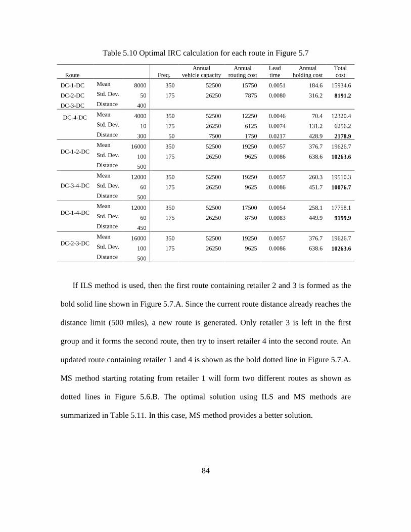
84

Table 5.10 Optimal IRC calculation for each route in Figure 5.7

Route Freq. Annual

vehicle capacity Annual

routing cost Lead time

Annual holding cost

Total cost

DC-1-DC Mean 8000 350 52500 15750 0.0051 184.6 15934.6

DC-2-DC Std. Dev. 50 175 26250 7875 0.0080 316.2 8191.2

DC-3-DC Distance 400

DC-4-DC

Mean 4000 350 52500 12250 0.0046 70.4 12320.4

Std. Dev. 10 175 26250 6125 0.0074 131.2 6256.2

Distance 300 50 7500 1750 0.0217 428.9 2178.9

DC-1-2-DC

Mean 16000 350 52500 19250 0.0057 376.7 19626.7

Std. Dev. 100 175 26250 9625 0.0086 638.6 10263.6 Distance 500

DC-3-4-DC

Mean 12000 350 52500 19250 0.0057 260.3 19510.3

Std. Dev. 60 175 26250 9625 0.0086 451.7 10076.7 Distance 500

DC-1-4-DC

Mean 12000 350 52500 17500 0.0054 258.1 17758.1

Std. Dev. 60 175 26250 8750 0.0083 449.9 9199.9 Distance 450

DC-2-3-DC

Mean 16000 350 52500 19250 0.0057 376.7 19626.7

Std. Dev. 100 175 26250 9625 0.0086 638.6 10263.6 Distance 500

If ILS method is used, then the first route containing retailer 2 and 3 is formed as the

bold solid line shown in Figure 5.7.A. Since the current route distance already reaches the

distance limit (500 miles), a new route is generated. Only retailer 3 is left in the first

group and it forms the second route, then try to insert retailer 4 into the second route. An

updated route containing retailer 1 and 4 is shown as the bold dotted line in Figure 5.7.A.

MS method starting rotating from retailer 1 will form two different routes as shown as

dotted lines in Figure 5.6.B. The optimal solution using ILS and MS methods are

summarized in Table 5.11. In this case, MS method provides a better solution.

85

Table 5.11 Optimal solution in Figure 5.7

Route IRC Frequency Vehicle usage Total cost

ILS method DC-1-2-DC 10263.6 175 61.0% 20340.3

DC-3-4-DC 10076.7 175 45.7%

MS method DC-1-4-DC 9199.9 175 45.7% 19463.5

DC-2-3-DC 10263.6 175 61.0%

5.3.4 Hybrid Genetic Algorithm Method (HGA)

A genetic algorithm (GA) is a search heuristic that mimics the process of natural

evolution. This heuristic is routinely used to generate useful solutions to optimization and

search problems. Genetic algorithms belong to the larger class of evolutionary algorithms

(EA), which generate solutions to optimization problems using techniques inspired by

natural evolution, such as inheritance, mutation, selection, and crossover.

Figure 5.8 HGA framework

The idea for the hybrid heuristic proposed here is to use a genetic algorithm (GA) to

generate/update a fixed partition for all retailers. A TSP is solved within each partition

86

and optimal delivery frequency is selected accordingly. In a fixed partition policy (FPP),

the retailers are partitioned into disjoint and collectively exhaustive sets. Each set of

retailers is served independently of the others and at its optimal replenishment rate. The

framework is shown in Figure 5.8, where GA is used to generate and update fixed

partition, TSP is solved by 2-opt heuristic.

Procedure

1. Set t = 0. Initialize Population P(t) with randomly constructed solutions. Alternatively

use results from heuristics (i.e., modified sweep method) as partial population.

2. Evaluate the feasibility and fitness function of individuals included in P(t).

3. Apply Crossover and Mutation operators to obtain a set C(t) of candidates that can

satisfy problem constraints.

4. Evaluate the set C(t) of candidate and select the best individuals with respect to

fitness value to add to new Population P(t+1). The new population consists of the best

PS (population size) chromosomes from P(t) and C(t).

5. t = t + 1, while stopping criteria are not met do, go back to step 2.

6. End and keep the best individual of the last population as the solution of the problem.

Chromosome Representation

In current research, the real number of vehicles used is an unknown variable, but the

maximum number will be the number of retailers. In that case, each retailer is serviced by

one individual route. The length of a chromosome is equal to the number of retailers N.

Each gene of the chromosome is related to a retailer and is assigned to an integer number

87

between 1 and N. If the ith gene is assigned to integer m, for instance, then it means that

retailer i is served by vehicle m.

1 2 3 4 5 6 7 8 9 10

2 1 4 2 1 1 4 3 3 2

The above chromosome represents a 4-vehicle solution, vehicle 1 services retailer 2, 5

and 6, vehicle 2 services retailer 1, 4 and 10, etc.

Chromosome Justification

The chromosome representation introduced above is easy to understand, but there will be

an issue in practice. For example, the following two chromosomes actually represent the

same solution. It’s a 4-vehicle solution with one vehicle services retailer 1,4,10; one

vehicle services retailer 2,5,6, one vehicle services retailer 8,9 and one vehicle services

retailer 3,7.

1 2 3 4 5 6 7 8 9 10

2 1 4 2 1 1 4 3 3 2

5 1 3 5 1 1 3 2 2 5

The differences in chromosomes' representations come from the order of different

routes. To deal with this symmetry and make the further calculation easier, a

chromosome justification is done every time after generating a new chromosome.

Justification: Number retailers from 1 to N. Following the order of retailers, each

retailer is assigned to the smallest available vehicle number.

By adopting this justification, the above two chromosomes will be modified to:

1 2 3 4 5 6 7 8 9 10

1 2 3 1 2 2 3 4 4 1

88

Crossover

Crossover is a mechanism in which the information between two chromosomes is

exchanged randomly. Two-point crossover operator is used, for example:

1 2 3 4 5 6 7 8 9 10

1 2 3 1 2 2 3 4 4 1

1 2 3 4 2 1 5 4 5 3

After crossover:

1 2 3 4 5 6 7 8 9 10

1 2 3 4 2 1 3 4 4 1

1 2 3 1 2 2 5 4 5 3

Additionally, one-point crossover operator can also be used, for example:

1 2 3 4 5 6 7 8 9 10

1 2 3 1 2 2 3 4 4 1

1 2 3 4 2 1 5 4 5 3

After crossover:

1 2 3 4 5 6 7 8 9 10

1 2 3 1 2 1 5 4 5 3

1 2 3 4 2 2 3 4 4 1

Mutation

In a mutation operator, each gene can change to a different integer number with a defined

probability, two examples:

1 2 3 4 5 6 7 8 9 10

1 2 3 1 2 2 3 4 4 1

Example 1

1 2 3 4 5 6 7 8 9 10

1 2 3 1 4 2 3 4 4 1

Example 2

1 2 3 4 5 6 7 8 9 10

1 2 3 1 5 2 3 4 4 1

89

In the first example, the number of routes does not change, but the real routes change.

In the second example, by assigning retailer 5 to route 5, the original 4-route solution

becomes a 5-route solution. Also check if justification is necessary whenever a new

chromosome is generated.

Fitness Function (ff)

The fitness score is a possibly-transformed rating used by the genetic algorithm to

determine the fitness of individuals for mating. In this heuristic, the objective function

value (total cost) is used directly as fitness score. It is probabilistically possible for

infeasible solutions to survive. A penalty value (a big positive number M) is applied to

the fitness function without removing infeasible solutions. The logic behind this is that an

optimal solution may exit with high probability near an infeasible solution. However, at

the same time, the proposed algorithm will record the best feasible solution. Since the

fitness function here is the total cost, the smaller the value is, the better the chromosome.

Selection

The roulette wheel selection operation is adopted to choose chromosomes to undergo

genetic operations. The approach is based on an observation that a roulette wheel has a

section allocated for each chromosome in the population, and the size of each section is

proportional to the chromosome’s fitness: the fitter the chromosome, the higher the

probability of being selected. Although one chromosome has the highest fitness, there is

no guarantee it will be selected. On average, a chromosome will be chosen with the

90

probability proportional to its fitness. Suppose the population size is PS, then the

selection procedure is as follows:

1. Calculate the total fitness of the population as FF.

2. Calculate the selection probability spi for each chromosome Xi: ( )

( 1)i

i

FF ff Xsp

FF PS

−=

−

3. Calculate the cumulative probability qpi for each chromosome Xi: 1

i

i jj

qp sp=

=∑

4. Generate a random number r from a uniform distribution in the range (0, 1].

5. If 1i iqp r qp− < ≤ , then chromosome Xi is selected.

Traveling Salesman Problem (TSP)

In the first stage, retailers are grouped into several sets and each set is serviced by one

vehicle. Within each set, use 2-opt search method to optimize the delivery tour and a

delivery frequency is selected later. For example, by solving TSP, the final solution is:

Route 1: {1, 4, 10} DC-4-10-1-DC

Route 2: {2, 5, 6} DC-2-6-5-DC

Route 3: {3, 7} DC-3-7-DC

Route 4: {8, 9} DC-8-9-DC

The total cost can be calculated based on the final routing schedule after selecting

delivery frequency for each route.

91


To evaluate the performance of the proposed four heuristics, an all direct-shipping

method is used to calculate upper bound. Total cost estimation and a lower bound are

generated using methods introduced in Section 5.2.


Parameter settings are defined in Tables 5.12 and 5.13.

Table 5.12 Parameter settings in phase II

Name Notation Value Remark Service level zα 1.96 97.50% Vehicle capacity C 150 Distance limit D 500 miles Vehicle speed s 500 miles/day Fixed cost a $ 5/truck Variable routing cost cd c = $ 0.1mile d = distance (miles) Available frequency/year fn {25, 50, 175, 350} 1year = 350 days Location of DC 0 (0, 0) Number of retailers N {20, 50, 100, 150, 200} Locations of retailers (x, y) [-100, 100] Uniform Distribution Demand mean/year

rµ 10% Low: [50, 150] 80% Medium: [500, 2000] 10% High: [10000, 25000]

Uniform Distribution

Demand standard deviation/year rσ Low: [1, 5]

High: [10, 50] Uniform Distribution

Holding cost hr Low: $ 10/unit year Medium: $ 50/unit year High: $ 100/unit year

Retailers are assumed to be randomly located in a 200-mile by 200-mile square with

the DC in the center. Number of retailers, holding cost and demand standard deviation

were variables shown in Table 5.9 to form 30 scenarios. Mean retailer demand, service

level, vehicle capacity and speed, distance limit (length of daily tour), location of DC,

and fixed truck cost were held constants. Vehicle capacity is set to be 150, this value is

roughly estimated so that one vehicle is used to serve about 10 retailers every two days

92

(Average demand/10 ≈150). Deliveries may be made daily, every other day, weekly, or

biweekly. Additional parameters were set for the TS-SA and HGA procedure as in Table

5.14. These were selected based on preliminary experimentation.

Table 5.13 Scenarios construction in Phase II

Scenario (k) N hr σr Scenario (k) N hr σr

1 20 High High 16 20 Medium Low 2 50 High High 17 50 Medium Low 3 100 High High 18 100 Medium Low 4 150 High High 19 150 Medium Low 5 200 High High 20 200 Medium Low 6 20 High Low 21 20 Low High 7 50 High Low 22 50 Low High 8 100 High Low 23 100 Low High 9 150 High Low 24 150 Low High 10 200 High Low 25 200 Low High 11 20 Medium High 26 20 Low Low 12 50 Medium High 27 50 Low Low 13 100 Medium High 28 100 Low Low 14 150 Medium High 29 150 Low Low 15 200 Medium High 30 200 Low Low

Table 5.14 Heuristics parameter settings in phase II

TS-SA Hybrid GA Name Value Name Value T0 1500 Population size 2N FT 10 Elite proportion 0.05 α Uniform: [0.7, 1.0] Mutation probability 0.05 MaxNum 500 TG 3000 NOIMPROVE 5 SG 100


Five random instances were generated for each experiment scenario. All four heuristics

were then applied to each instance, and results in the following tables for each scenario

are the average of those five random instances. For meta-heuristics, the maximum

running time was set to be 3600 seconds (1 hour). All the computational times are

obtained on a Intel(R) Core(TM)2 T5550 at 1.83 GHz using Windows 7.

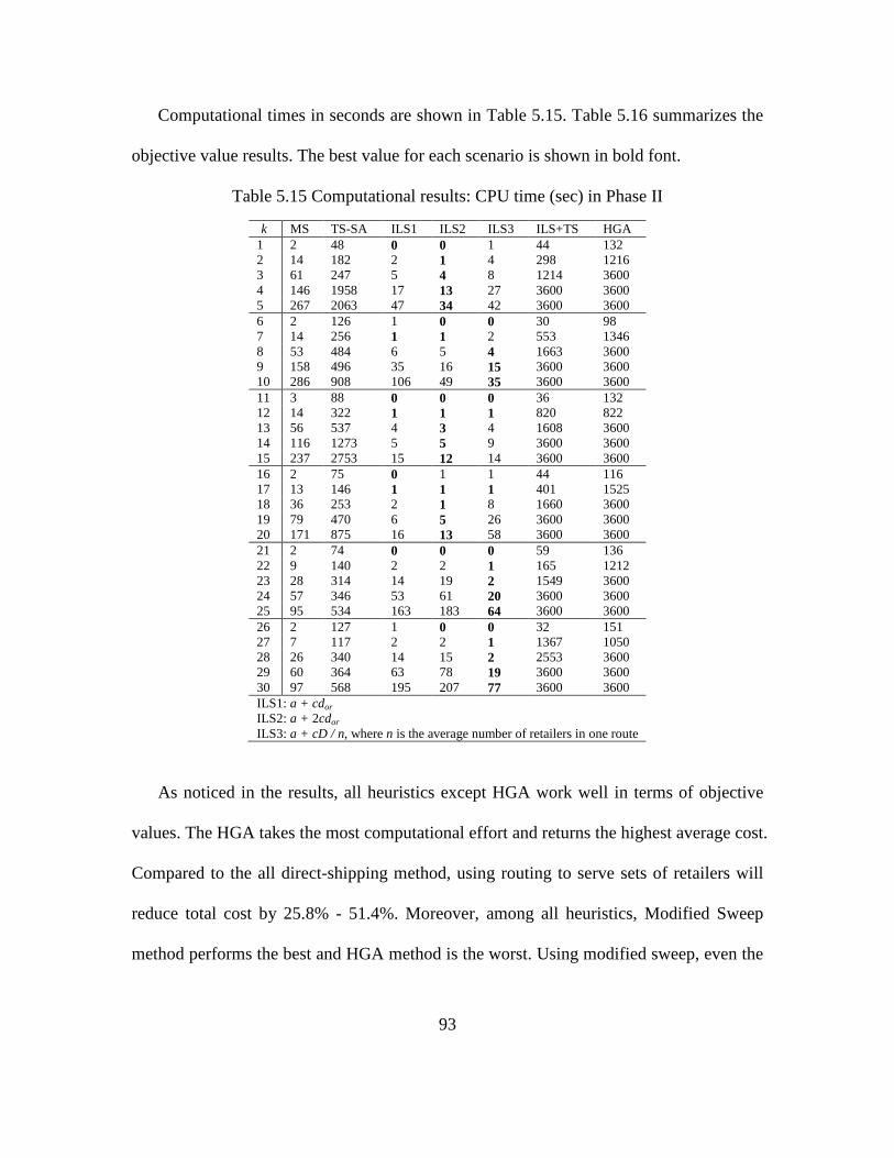
93

Computational times in seconds are shown in Table 5.15. Table 5.16 summarizes the

objective value results. The best value for each scenario is shown in bold font.

Table 5.15 Computational results: CPU time (sec) in Phase II

k MS TS-SA ILS1 ILS2 ILS3 ILS+TS HGA 1 2 48 0 0 1 44 132 2 14 182 2 1 4 298 1216 3 61 247 5 4 8 1214 3600 4 146 1958 17 13 27 3600 3600 5 267 2063 47 34 42 3600 3600 6 2 126 1 0 0 30 98 7 14 256 1 1 2 553 1346 8 53 484 6 5 4 1663 3600 9 158 496 35 16 15 3600 3600 10 286 908 106 49 35 3600 3600 11 3 88 0 0 0 36 132 12 14 322 1 1 1 820 822 13 56 537 4 3 4 1608 3600 14 116 1273 5 5 9 3600 3600 15 237 2753 15 12 14 3600 3600 16 2 75 0 1 1 44 116 17 13 146 1 1 1 401 1525 18 36 253 2 1 8 1660 3600 19 79 470 6 5 26 3600 3600 20 171 875 16 13 58 3600 3600 21 2 74 0 0 0 59 136 22 9 140 2 2 1 165 1212 23 28 314 14 19 2 1549 3600 24 57 346 53 61 20 3600 3600 25 95 534 163 183 64 3600 3600 26 2 127 1 0 0 32 151 27 7 117 2 2 1 1367 1050 28 26 340 14 15 2 2553 3600 29 60 364 63 78 19 3600 3600 30 97 568 195 207 77 3600 3600 ILS1: a + cdor

ILS2: a + 2cdor

ILS3: a + cD / n, where n is the average number of retailers in one route

As noticed in the results, all heuristics except HGA work well in terms of objective

values. The HGA takes the most computational effort and returns the highest average cost.

Compared to the all direct-shipping method, using routing to serve sets of retailers will

reduce total cost by 25.8% - 51.4%. Moreover, among all heuristics, Modified Sweep

method performs the best and HGA method is the worst. Using modified sweep, even the

94

largest case, it only takes 2 minutes and finds a good solution. But HGA takes a long time

and generates worse solutions. Two major reasons may explain this result:

Table 5.16 Computational results: Objective values ($1000) in Phase II

k MS TS-SA ILS1 ILS2 ILS3 ILS+TS HGA Lower bound IRCe

Direct shipping

1 45.0 47.3 58.8 56.6 52.3 47.5 45.3 30.8 41.0 71.9 2 99.5 110.6 128.2 131.9 121.2 97.2 109.7 63.4 99.0 174.0 3 198.2 215.2 260.2 271.8 233.0 200.9 250.8 123.9 207.0 363.9 4 288.6 285.7 388.5 409.2 364.4 290.2 347.6 173.7 307.2 548.0 5 373.5 375.1 509.9 525.3 434.7 374.3 485.5 217.4 401.3 723.5 6 33.4 34.5 42.0 37.2 47.3 33.9 35.0 20.8 30.5 57.7 7 84.6 93.0 107.9 109.5 107.2 86.6 91.0 50.3 81.6 152.8 8 145.0 150.2 186.3 200.2 194.9 148.5 175.3 81.8 153.8 279.3 9 200.8 215.3 292.3 285.0 267.3 205.3 224.3 114.2 228.9 413.1 10 271.9 272.3 385.8 381.4 358.2 270.3 347.2 148.3 307.4 555.0 11 37.5 38.2 43.4 46.4 57.4 38.6 37.0 23.4 30.8 52.6 12 68.0 71.4 83.2 88.3 95.1 68.0 77.4 41.8 68.8 114.3 13 138.9 138.0 166.2 169.7 175.7 135.7 160.3 74.9 140.2 235.5 14 214.1 214.5 253.6 265.6 285.1 215.1 264.1 111.4 217.0 369.7 15 274.8 248.0 330.5 347.9 347.7 268.9 351.1 139.3 284.4 482.3 16 30.3 31.5 35.1 36.9 41.8 30.4 29.7 18.2 23.1 42.4 17 80.8 83.6 95.5 99.4 98.1 81.9 87.1 41.9 66.4 119.5 18 142.9 148.3 163.2 167.0 175.6 133.3 175.3 65.8 119.5 217.2 19 209.5 209.3 242.8 249.8 260.6 200.3 233.1 92.7 180.0 325.8 20 248.4 244.6 302.1 311.7 307.6 234.3 333.9 107.7 225.5 408.5 21 16.2 16.9 18.3 18.3 23.6 16.4 17.9 8.7 10.9 23.0 22 36.8 39.3 42.6 42.6 47.6 37.1 38.8 18.4 26.1 55.4 23 76.3 76.6 90.3 85.9 92.0 70.1 90.2 34.5 53.7 112.1 24 108.5 116.9 128.7 125.3 145.0 102.3 143.4 47.2 80.0 163.5 25 149.8 156.1 176.9 174.6 194.1 140.2 191.6 61.9 109.0 224.5 26 16.2 17.1 18.7 17.8 24.4 17.2 16.5 9.0 10.0 21.8 27 34.2 36.3 39.9 38.9 50.0 34.6 38.4 16.3 22.6 50.4 28 65.2 68.2 78.8 77.4 81.9 64.1 70.3 34.6 56.6 100.0 29 99.4 108.5 118.3 119.0 138.8 96.1 136.2 45.5 80.1 153.8 30 139.7 146.9 164.7 163.8 169.0 134.7 188.1 50.7 91.6 214.6

1. Even the modified sweep method is straightforward, it has some theoretical

foundation and captures many important aspect of this routing problem. In the

problem, it has distance and capacity constraints, and it is preferred to merge

proximate retailers together for the consideration of shipping. Thus the method

sweeps all retailers clockwise and counterclockwise. Every time deciding whether or

not to insert a new retailer, the route is modified and 2-opt is used to improve the

95

route tour. In addition, joint tours and separate frequency tours are compared to find a

better solution.

2. HGA method works by making improvement from operators (crossover, and

mutation). However, there is a high probability that a child is infeasible with capacity

and distance constraints, especially in large instances. If allowing the HGA to run

infinitely, it may find the best solution, but this is not efficient.

LS works very fast in terms of CPU time, but its objective values are much higher

than MS. If joint with Tabu search, ILS-TS generates better results than MS in large

scenarios, but CPU time increases because of Tabu search step. So MS method is

recommend for IRP in this research stage, and Tabu search method can be used to further

improve results from MS method if necessary.

The saving percentage (1 - best solution / direct-shipping cost) is shown in Table 5.17.

When the holding cost and demand variance decrease, the benefits from routing strategy

decrease. Retailers will prefer to order more products each time when their inventory cost

is lower, so the number of retailers in one route will decrease because of capacity

limitation. In the extreme case, when the number of retailers in one route is only one, this

is equivalent to direct-shipping. Routing strategy will have more benefits if the demand

or optimal order size of each retailer is small compared to vehicle capacity.

Table 5.17 Saving percentage in Phase II

hr σr N = 20 N = 50 N = 100 N = 150 N = 200 Average High High 37.4 44.2 45.5 47.9 48.4 44.7 High Low 42.1 44.6 48.1 51.4 51.3 47.5 Medium High 29.7 40.5 42.4 42.1 48.6 40.7 Medium Low 29.9 32.3 38.6 38.5 42.6 36.4 Low High 29.6 33.7 37.5 37.2 37.6 35.1 Low Low 25.8 32.2 35.9 37.5 37.2 33.7

96

6. INTEGRATED PROBLEM’S RESULTS AND ANALYSIS

To sum up, the original integrated problem is decomposed into two phases. The DC’s

locations and PW/retailer’s assignments are determined in the first phase using IRC

heuristic described in Section 4.5.2. The actual routing decisions are determined in the

second phase using modified sweep method.

Figure 6.1 Solution methodology

In this Chapter, the integrated problem is solved using the proposed methods as

shown in Figure 6.1. Eight different data sets tested in phase I are used here, all

parameter settings are the same as in Table 4.1. Table 6.1 summarizes results from all

experiments including objective value, computational time, and the number of opened

DCs and the number of total routes under each scenario.

Table 6.1 Computational results for the integrated problem

Original Solution

Objective Value

CPU time (sec) No. DCs

Approx. IRC

Real IRC

Total cost

No. Routes

Total CPU time

IRC Gap

1 60928 58176 44 2 33942 31504 55738 5 49 0.07

2 142006 122790 482 2 83963 81575 120403 16 617 0.03

3 337704 271723 1408 4 181252 183543 274014 36 1854 0.01

4 418300 326696 959 3 223307 239583 342972 51 1592 0.07

5 799990 484503 1592 4 325656 336614 495461 57 2569 0.03

6 65618 60717 10 1 37077 36122 59761 7 16 0.03

7 137905 103029 105 1 74460 76163 104732 15 221 0.02

Original network design problem

Phase I: FLP with approximate IRC

DC locations and retailer assignments

Phase II: IRP, route assignments

Each opened DC

97

Original Solution

Objective Value


Approx. IRC

Real IRC

Total cost

No. Routes

Total CPU time

IRC Gap

8 345284 254270 1298 4 159298 153504 248476 25 1405 0.04

9 440717 339563 1427 4 223461 231161 347263 44 1889 0.03

10 661228 463149 1753 6 283359 266003 445793 43 2028 0.06

11 73881 70881 54 2 30280 28220 68821 4 59 0.07

12 175279 141923 568 2 84838 87967 145053 18 591 0.04

13 357440 238344 1051 2 156586 163545 245304 34 1236 0.04

14 482040 367739 1540 5 217478 199291 349553 31 1944 0.08

15 861397 452389 2543 2 317889 355398 489898 78 3612 0.12

16 43258 37529 8 1 24559 25596 38566 7 14 0.04

17 110527 93771 93 2 55761 53841 91851 13 188 0.03

18 233572 167867 552 2 110799 114481 171549 37 649 0.03

19 327009 229206 1325 2 155542 167072 240736 51 2015 0.07

20 580662 342172 1654 4 215101 211163 338234 56 1962 0.02

21 41026 41026 31 2 20784 17350 37593 5 37 0.17

22 103359 89303 177 3 49928 47246 86621 13 250 0.05

23 251714 178622 806 2 112316 112373 178679 33 963 0.00

24 315053 250057 1124 2 167901 187029 269185 71 1575 0.11

25 595000 364909 1740 3 218522 223647 370034 65 2965 0.02

26 47835 44687 19 1 24897 23232 43022 5 23 0.07

27 124696 100579 381 2 55020 52409 97967 15 578 0.05

28 255065 191070 1377 3 105105 106414 192379 32 1562 0.01

29 363452 277301 1517 4 155055 156860 279106 44 2161 0.01

30 696137 363754 1449 3 220151 233431 377034 67 2197 0.06

31 66558 65313 32 2 40398 35705 60620 5 36 0.12

32 159410 138424 75 1 100617 104052 141858 21 149 0.03

33 446165 346922 1262 4 204297 205194 347820 32 1314 0.00

34 529884 389906 1187 2 277816 315980 428071 60 1917 0.14

35 894131 545477 1635 4 339706 358123 563894 65 1941 0.05

36 74593 69096 11 1 44309 41705 66492 8 17 0.06

37 198341 176813 575 2 109408 112236 179642 17 598 0.03

38 433334 344253 2182 3 220242 243334 367344 51 2301 0.10

39 551753 412235 1381 2 290029 319810 442016 57 3224 0.10

40 1001097 569713 1748 5 335786 339643 573570 55 2080 0.01

41 70061 68748 13 1 36635 36087 68200 9 20 0.01

42 176209 148289 539 2 91294 86254 143249 13 572 0.06

43 511315 373717 1325 3 217132 231837 388422 38 1470 0.07

44 595933 460701 1464 3 286737 292370 466334 47 2062 0.02

45 1029142 637322 1134 3 394111 431764 674975 77 3112 0.10

46 55017 49203 11 1 33857 51052 66398 11 18 0.51

98

Original Solution

Objective Value


Approx. IRC

Real IRC

Total cost

No. Routes

Total CPU time

IRC Gap

47 151329 140380 152 3 73763 73081 139698 15 230 0.01

48 314144 231574 1358 3 139551 139573 231595 35 1441 0.00

49 477297 372730 980 3 208845 221223 385109 50 1702 0.06

50 784966 409663 1651 3 258329 281449 432783 69 2728 0.09

51 59667 52792 14 1 33358 36000 55434 9 21 0.08

52 165152 135331 177 2 75009 76922 137244 18 258 0.03

53 285721 217315 1303 2 128515 141001 229801 37 1974 0.10

54 451527 345879 1436 3 204110 218322 360091 55 1903 0.07

55 821873 465626 2195 4 261308 264659 468976 64 2501 0.01

56 49168 44449 19 1 23577 24997 45869 8 28 0.06

57 141823 123224 709 2 67285 66631 122570 15 733 0.01

58 316108 236447 1419 3 128098 138527 246876 39 1564 0.08

59 476277 361695 1531 3 197979 207134 370850 55 2052 0.05

60 869445 510900 1480 4 270102 292256 533054 67 2297 0.08

61 68884 65359 48 2 36790 36539 65108 7 53 0.01

62 176373 157944 214 3 89204 86801 155541 15 233 0.03

63 380172 279400 1061 4 161550 160374 278224 31 1141 0.01

64 556114 413921 1298 3 243718 244947 415150 43 1923 0.01

65 1075650 561637 1216 4 330483 333247 564401 55 2255 0.01

66 59810 52715 9 1 29741 25959 48933 4 15 0.13

67 190322 136632 280 2 80394 77235 133474 11 433 0.04

68 430563 263430 1357 2 160774 164559 267216 35 1949 0.02

69 549299 392281 1072 2 247815 263725 408191 58 1557 0.06

70 1157796 527163 1850 4 293683 287166 520647 45 2691 0.02

71 79361 67570 8 1 31717 28529 64382 6 14 0.10

72 183478 147635 442 2 78455 75119 144299 14 600 0.04

73 439712 282332 2067 3 157786 155197 279743 34 2251 0.02

74 566400 399406 1562 2 241076 262587 420917 52 2242 0.09

75 1101735 544567 1533 4 305017 306107 545657 59 2697 0.00

76 50857 49529 33 2 22977 22002 48554 6 37 0.04

77 133244 97220 491 2 54692 50370 92898 14 804 0.08

78 325846 175547 904 2 106017 104619 174149 27 1488 0.01

79 420871 300592 1393 3 164574 166429 302448 51 2198 0.01

80 883370 380826 1618 3 208382 219057 391501 61 2846 0.05

81 53905 52568 194 2 22816 20418 50170 6 199 0.11

82 145144 111693 767 2 57074 56143 110762 13 791 0.02

83 344524 229454 786 3 111195 113164 231422 33 915 0.02

84 452943 341346 1126 4 166998 169877 344226 53 1507 0.02

85 858688 365487 2159 3 202221 213825 377090 68 3225 0.06

99

Original Solution

Objective Value


Approx. IRC

Real IRC

Total cost

No. Routes

Total CPU time

IRC Gap

86 58814 58340 66 2 21095 19257 56503 5 71 0.09

87 146010 114123 929 2 56966 56882 114040 19 1048 0.00

88 354070 245455 1460 3 115918 123950 253487 38 1668 0.07

89 427952 315837 1245 3 147621 150314 318530 43 1839 0.02

90 946959 420331 1870 3 203085 215803 433049 72 3037 0.06

91 90095 88531 16 2 46324 41522 83728 6 20 0.10

92 194878 152264 1968 2 94102 92598 150760 17 1988 0.02

93 565169 403239 923 3 232386 230682 401535 35 1258 0.01

94 687053 486360 1067 3 273021 288834 502174 56 1899 0.06

95 1381632 596740 1552 2 400505 460236 656471 93 2325 0.15

96 84364 76619 8 1 44045 45720 78294 7 15 0.04

97 195399 170204 541 3 89711 87560 168052 17 557 0.02

98 539073 358524 940 2 221165 225821 363180 41 1060 0.02

99 836530 605684 1411 4 300269 313480 618895 49 1791 0.04

100 1315789 629805 1747 4 323144 338145 644807 55 2170 0.05

101 88119 80613 9 1 40446 41254 81421 9 16 0.02

102 233553 181776 693 2 93957 95525 183345 14 715 0.02

103 631148 400342 1233 2 218564 227752 409530 35 1396 0.04

104 824451 622704 1522 6 276346 299861 646219 38 1624 0.09

105 1302067 579574 1371 3 317838 329613 591349 60 2243 0.04

106 69782 54977 9 1 28125 28599 55451 7 16 0.02

107 189229 148684 264 2 69788 65991 144888 16 466 0.05

108 455272 266417 1353 3 129473 133334 270279 30 1873 0.03

109 778168 512949 1092 3 238546 276429 550832 68 1598 0.16

110 1202676 559753 1605 3 290054 318230 587929 76 2584 0.10

111 88432 72994 8 1 39926 44767 77834 11 15 0.12

112 155882 122214 603 2 60756 58637 120095 18 627 0.03

113 375032 239700 1365 3 123190 125046 241556 37 1459 0.02

114 607656 435270 1497 3 215448 240494 460315 62 2218 0.12

115 1506312 590362 1661 3 282277 315914 623998 74 2499 0.12

116 74736 63866 9 1 34180 31076 60762 8 15 0.09

117 196019 150043 1328 2 75141 79349 154252 22 1476 0.06

118 447562 302342 1056 3 137973 142494 306863 36 1217 0.03

119 801576 550683 1146 3 217214 233387 566856 50 2001 0.07

120 1277470 637893 1349 4 267297 291807 662403 66 1980 0.09

From the experimental results for the integrated problem shown in Table 6.1, the

following observations are observed:

100

1. All instances are solved in a reasonable time by the heuristics, with the maximum

computation time of one hour (3612 seconds in scenario 15).

2. Heuristics work well in terms of objective values compared to the original greedy

solution. The original greedy solution’s value is reduced by 25.3% on average.

3. The IRC gap in the table is calculated as |Real IRC/Approximated IRC - 1|. The

average value for this gap is 5.6%. This indicates the approximate cost function for

IRC constructed in Chapter 4 provides a good fit to the actual IRC in the integrated

problem.

4. From the number of retailers and the number of routes used for delivery, there are on

average 3 to 5 retailers in one route. There are still some retailers using individual

route delivery from the detailed routing information. This is why using the average

value of possible routing cost and direct shipping cost ( ( ) / 2ji ji jir α β= + in Section

4.1, αji is the routing cost using nearest neighborhood insertion method for retailer i

from DC j and βji is the direct shipping cost for retailer i from DC j) as the routing

parameter r ji is found in empirical studies to more closely approximate solutions than

using routing cost αji alone.

For example, Table 6.2 records the running results for the first 15 scenarios if only

routing cost αji is used and Table 6.3 records the running results for the first 15

scenarios if only direct shipping cost βji is used. The average IRC gaps in these two

cases become 14.4% and 32.8% separately, these two values are large and indicate

inaccuracy of estimated IRC.

101

Table 6.2 Computational results for the integrated problem if only routing cost αji is used

Original Solution

Objective Value


Approx. IRC

Real IRC

Total cost

No. Routes

Total CPU time

IRC Gap

1 43026 37364 12 1 23781 20521 34104 3 19 0.14

2 115974 95176 350 2 62798 64894 97272 16 493 0.03

3 246788 175265 1299 3 122301 137426 190390 36 1784 0.12

4 327825 228772 1384 2 160612 193446 261606 44 2457 0.20

5 616569 343016 1243 4 233923 347391 456485 46 2408 0.49

6 52543 49934 432 2 26958 22202 45179 5 438 0.18

7 131854 88561 106 1 62314 66808 93055 17 228 0.07

8 270301 180150 928 4 110066 106981 177065 21 1058 0.03

9 329369 251674 935 2 184990 209318 276002 45 1626 0.13

10 632161 343345 1825 4 227234 264920 381031 64 3216 0.17

11 62460 62420 26 2 26535 21807 57692 6 33 0.18

12 220621 214335 361 2 124550 119482 209267 16 543 0.04

13 271742 180809 1129 2 113867 130528 197470 34 1367 0.15

14 376550 583347 1132 3 368449 393092 607990 57 1861 0.07

15 708067 336230 1486 3 206430 240520 370321 49 2728 0.17

Table 6.3 Computational results for the integrated problem if only direct shipping cost βji is used

Original Solution

Objective Value


Approx. IRC

Real IRC

Total cost

No. Routes

Total CPU time

IRC Gap

1 79648 68162 10 1 43067 50915 76010 5 18 0.18

2 188584 164943 266 2 107386 136509 194066 24 401 0.27

3 442915 333540 848 3 201330 270447 402657 35 924 0.34

4 626553 461071 1779 3 296029 427001 592044 56 2310 0.44

5 1138800 611697 1651 4 341453 492463 762707 68 2430 0.44

6 84658 75404 10 1 42482 49674 82596 6 16 0.17

7 201397 178192 97 2 98868 130662 209987 18 161 0.32

8 464876 324986 2055 2 211185 315717 429519 59 429519 0.49

9 639992 468034 1460 3 276531 380209 571713 47 2000 0.37

10 1066300 619865 1753 3 383099 553918 790684 93 2483 0.45

11 79604 79062 81 2 36567 43121 85616 7 87 0.18

12 220621 194624 171 2 112902 134132 215855 17 283 0.19

13 484423 352984 1345 4 185667 225817 393134 29 1397 0.22

14 666544 510598 1227 4 257921 346112 598790 35 1859 0.34

15 1182180 621347 2553 3 341757 519640 799230 82 3741 0.52

102

In this research, whether the location decision is accurate depends on how the

estimated IRC compared to the actual IRC. There are two ways to increase this accuracy,

one is to update IRC for each retailer to its assigned DC in current solution each time and

the other is to update weights to parameters α, β. In the first case, only the related IRC for

each retailer to its assigned DC can be updated and this value also depends on other

retailers assignments (because of the route generation). For example, there are two DCs

and five retailers, retailers 1, 2 and 3 are assigned to DC 1 and retailers 4 and 5 are

assigned to DC 2 in current solution. Then only related IRC (α11, α12, α13, α24, α25) can be

updated and these valued are only accurate in current assignment solution. This will make

the iteration nonsense or too inefficient. So instead of updating IRC at each time, the

more efficient way is to consider selecting or updating the weights to parameters α, β. By

comparing the estimated IRC and actual IRC, the closer these two values are, the more

accurate the location decision is.

The actual routing structure depends on the location density (the retailer’s distance to

its nearest neighbor compared to the routing distance limit) and the demand density (the

individual’s annual demand rate compared to the routing vehicle’s capacity). Prior

knowledge will provide better estimation about the IRC in phase I. If retailers are close to

each other and each retailer’s annual demand rate is relatively small, then higher weight

should be given to the possible routing cost when estimating routing parameters.

Otherwise, higher weigh should be given to the direct shipping cost. To estimate a more

accurate routing cost r ji, the following formula is proposed:

r ji = w αji + (1-w) βji (6-1)

103

,D C

w fd µ

=

(6-2)

Equation (6-1) states that the routing cost r ji is a weighted average of αji (the routing

cost using nearest neighborhood insertion method) and βji (the direct shipping cost).

Equation (6-2) states that the weight w is a function of location density (d : the average

distance to nearest neighbors; D: routing distance limit) and the demand density (µ : the

average annual demand; C: the routing vehicle’s capacity C). The numerical relationship

is undefined and should become one future research direction. But in general, an

approximate weight value can be found by the binary search method until a predefined

acceptable gap value is achieved.

104

7. CONSOLIDATION FACILITY LOCATION AND DEMAND ALLOCATI ON

MODEL (CFLDAM)

Chapter 3 through 6 derived an integrated model for the proposed multi-product supply

chain network design problem with location, inventory and routing decisions, and then

generated a two-phase solving methodology for the complex model.

One distinguishing part in this proposed problem is to include transhipments between

DCs. A transhipment network is a realistic representation of many real world problems

that have a general network structure with many supply/demand points and

interconnecting links, and this network structure is not usual in available research work.

In this chapter, another model of designing a distribution network which also acquires

products from multiple facilities and then delivers products to retailer is introduced.

Different to previous models, this problem is formulated with direct shipment and

consolidation opportunities. Even though it is still a multi-product system, the

transhipment option does not exist and each production facility ships its product directly

to each opened DC. Another innovation structure motivated from many real world

problems is to group products into different sets based on environmental or other factors

is generated. Consolidation is allowed for shipping products in the same product set, but

products from different product sets must be shipped separately.


This chapter considers the selection of DC locations and sizes from a predetermined

finite set of options and the subsequent choice of distribution paths from multiple product

suppliers to retailers in a three-echelon supply chain (facility, DC and retailer) system.

105

The objective is to optimize the whole system and minimize the total cost which includes

fixed location cost, inventory cost and transportation cost. Two shipment methods are

considered for products to each retailer: direct shipment from facility to retailer and

indirect shipment from facility to DC and then from DC to retailer. Moreover, multiple

products are grouped into sets based on environmental or other factors and allow

consolidation in transportation. With respect to inventory, both safety stock and regular

inventory are included and the trade-off between inventory and transportation costs when

delivery time requirements must be met or replaced by safety stock is considered.

Production facilities already exist and each provides one specific product. DCs can be

located at potential locations with alternative sizes and need hold both cycle inventory

and safety stock. They may also effectively serve as cross-docking points. Retailers’

locations are also known in advance and the demand rate for each product at each retailer

is assumed to have a known distribution per time (assumed later to be normally

distributed for simplicity of presentation). Each retailer can order from a DC or directly

from manufacturers but chooses a single route for each product. In practice, this decision

is based on cost and delivery lead time. In addition to regular cycle inventory, retailers

hold safety stock if the lead-time of replenishing one order is above a specific threshold

value (for example, one day).

Products are divided into sets based on environmental or other factors. Consolidation

is allowed for shipping products in the same product set, but products from different

product sets must be shipped separately. The holding cost rate for products is the same

for products in the same set. For instance, in a food chain, certain products may require

106

refrigerated trucks. In other environments security or handling considerations may dictate

compatibility of products.

Different notation to previous chapters is used in this new problem and is described as

follows:

Index sets

I set of products

S set of product sets

K set of DCs

J set of possible DC sizes–small, medium and large

R set of retailers

N set of subscripts, n = 1, …, 5, where 1 means from a facility to a retailer, 2

means from a facility to a DC, 3 means from a DC to a retailer, 4 means at a DC, 5

means at a retailer

Parameters

kjf fixed cost of opening one DC at location k with size j

kjU capacity of one DC at location k with size j

nijlt lead time from point i to j (n = 1, 2, 3)

nijC capacity of one truck used for shipping from point i to j (n = 1, 2, 3)

nijA setup cost of each order from point i to j (n = 1, 2, 3)

107

nija fixed transportation cost per trip for using one truck from point i to j (n =

1, 2, 3)

nijbl variable transportation cost from point i to j (n = 1, 2, 3)

nijh holding cost of product i at point j per time (n = 4, 5)

srh holding cost of product set S at retailer r

nijt 1 if the lead time from point i to j is greater than threshold value (one day),

0 otherwise (n = 1, 3)

irD demand mean of product i at retailer r per time

2irσ demand variance of product i at retailer r

Decision Variables

kjw 1 if opening one DC at location k at size j, 0 otherwise

irx 1 if retailer r orders product i from facility i directly, 0 otherwise

ikrx 1 if retailer r orders product i from DC k, 0 otherwise

nijQ quantity of one order of product i from the facility to j (n = 1, 2)

3ikrQ quantity of one order of product i from DC k to retailer r

3skrQ quantity of one order of one product set s from DC k to retailer r

The objective is to minimize the total cost including: fixed DC location costs

(depreciation), regular inventory cost, safety stock cost, order cost and transportation

cost. When calculating safety stock at a DC, risk-pooling is applied for each product. At a

108

DC, the total safety stock for one product is shown in Equation (7-1) and is determined as

the desired confidence multiplier times the standard deviation of cumulative product

demand served by that DC.

22i ir ik ikrr

SS z lt xα σ= ∑ (7-1)

When calculating the transportation cost, assume a fixed cost of using a truck per

shipment along with a variable cost related to number of units and shipping distance.

Thus, cost for each order is equal to: fixed cost ⋅number of trucks + variable cost ⋅

distance ⋅ quantity of one order. Assuming full truck load order size, the cost is shown in

Equation (7-2).

Transport Cost / Shipment = Q

a bl QC ⋅ + ⋅

(7-2)

An economic order quantity model is used to determine the initial optimal order

quantity. And since the existence of order cost, it is shown to be near optimal using

multiple full-truck loads at one time instead of sending one full-truck load several times.

Let Q0 be the optimal economic order quantity assuming fixed truck costs are linearized.

Due to the relative insensitivity of actual cost to quantity and the economics of full

truckload shipments, the actual order quantity used is selected from the floor or ceiling

function of Q0 as either 0 /Q Q C C = ⋅ or ' 0 /Q Q C C = ⋅ . Bounds on maximal loss from

considering only full truck loads are derived in the Appendix B. The model is easily

extended to allow for multiple capacity truck options in the case that the natural order

size is significantly different than the capacity of the normal truck for such shipments.

The modeller could include options for 20’, 40’ and 53’ containers for instance or even

109

smaller delivery trucks for local deliveries from DCs to retailers. Indeed, structurally,

options such as mail packages could even be considered.

Mixed Integer Programming Model

By using the defined notation and decision variables in previous section, the proposed

problem can be modelled as follows:

Minimize

2 42

4 2

3 1 5

5 3 3 1 1

11 1 1 1

1 1

2

2

ik iki

kj kj ik ir ik ikrk j k k i r

s skr r ir ir

k s iir ir kr ikr kr ir ir ir ir

r r i k

ir ir irir ir ir ir

i ir

Q hf w z h lt x

Q h Q hz h t x lt t x lt

Q D xA a bl Q

C Q

α

α

σ

σ σ

+ +

+ + + +

+ + +

∑∑∑ ∑ ∑∑ ∑

∑∑ ∑∑ ∑∑ ∑

∑ 22 2 2 2

2 2

33 3 3 3

3 3

ir ikrik r

ik ik ik ikr k iir ik ik

s ir ikrskr i S

kr kr kr kr sk r s kr kr

D xQ

A a bl QC Q

D xQ

A a bl QC Q

∈

+ + +

+ + +

∑∑ ∑∑

∑∑∑∑

(7-3)

Subject to:

2 ik kjj

Q Mw≤∑ ,i k∀ (7-4)

3 skr kj

j

Q Mw≤∑ , ,s k r∀ (7-5)

3 3skr ikr

i S

Q Q∈

=∑ , ,s k r∀ (7-6)

1kjj

w ≤∑ k∀ (7-7)

1ikr irk

x x+ =∑ ,i r∀ (7-8)

110

222 0.8

2ik

ir ik ikr kj kji i r j

Qlt x U wσ+ ≤∑ ∑ ∑ ∑ k∀ (7-9)

1 2 3, , 0sir ik krQ Q Q ≥ , , ,i s k r∀ (7-10)

{ }, 0,1ir ikrx x ∈ , ,i k r∀ (7-11)

The objective function (7-3) has six terms- the fixed DC location costs, the average

inventory costs at DCs, the average inventory costs at retailers, order cost, the

transportation cost from facilities to retailers directly, the transportation costs from

facilities to DCs and the transportation costs from DCs to retailers when needed. Safety

stock at a site is based on desired percentiles of its replenishment lead time demand.

When delivery lead time (distance) is below an acceptable threshold, safety stock is not

needed. The order quantities are computed by first finding the optimal continuous

economic order quantity and then costing out the options of that quantity against the

rounded up and down full truck load alternatives. Based on the choice of xir, xikr the

candidate continuous optimal order quantity value can be found using the typical EOQ

model as shown in Equations (7-12) to (7-14). As described above, these values are then

rounded to find the appropriate Q value for use in the model.

0 11

5

2 ir ir irir

ir

A D xQ

h= (7-12)

2

02

4

2 ik ir ikrr

ikik

A D x

Qh

=∑

(7-13)

111

3

03

2 kr ir ikri Ss

kr sr

A D x

Qh∈

=∑

, 0 03 3

s irikr kr

iri S

DQ Q

D∈

= ∑

(7-14)

The cost model is adaptable. For instance, suppose orders are for multiple truck loads.

The model above assumes all loads are shipped at once. However, if truck loads are

spaced in time by the ratio of truck capacity to demand, then the inventory terms in (7-3)

would be replaced by expressions of the form Ch / 2 (A similar change is used in

equation (7-9)).

Constraint sets (7-4) and (7-5) require that shipping quantities for one plant to one DC

or from one DC to one retailer can be greater than 0 only when opening this DC.

Constraint set (7-6) sets the total shipping quantity of one product set equal to the

summation of all the shipping quantities of products in this product set. Constraint set (7-

7) limits opening at most one DC at one potential DC location. Constraint set (7-8)

requires only one supplier for each retailer-product combination; the retailer can order

directly from the plant or order from one DC. Constraint set (7-9) assumes random access

and guarantees the average inventory level at each DC should be less than the effective

capacity of this DC. Average inventory includes cycle stock plus safety stock. Effective

capacity is nominally set at 80% of total space (but is easily adjusted). Average

inventory is equal to average cycle inventory plus a safety stock based on replenishment

lead time and total product volume. Constraints set (7-10) and (7-11) are nonnegative

and binary constraints.

112

7.2 Solution Methods

A genetic algorithm and construction heuristic are proposed and tested here.

7.2.1 Genetic Algorithms (GAs)

Deriving optimal or near-optimal solutions to location problems has fed the growth of the

field of location analysis over the past three decades (Jamarillo et al. 2002). The large

number of integer variables makes it computationally difficult to solve. For this reason a

genetic algorithm approach is applied.

In recent years, GAs have been used to solve several optimization problems, but

applications of GAs to location models have been relatively few. Hosage and Goodchild

(1986) and Chaudhry et al. (2003) present an application of GA for the p-median problem.

Gen and Syarif (2005) propose a spanning tree-based GA to solve a location facilities

problem considering multi products and multi periods. Finally, Jamarillo et al. (2002) and

Zhou et al. (2003) propose GA application to two simple models for location-allocation

problems. A GA application is presented for a complex model of location considering

several factories with single product production, several potential sites for opening DCs,

multiple customers having different and continuous demand for each product and the

choice of direct or indirect shipment from factories and retailers. In the next section, the

GA heuristic is presented in detail and then report the outcome of empirical tests.

Chromosome representation

The chromosome representing the problem solution is composed for each product by 3

sub-strings representing respectively: (i) the direct shipment of products from a single

113

factory to network’s retailers (i to r), (ii) the link among a single factory and the possible

sites for opening DCs (i to k), and (iii) the shipment of products from DCs to retailers (k

to r). (The i to k link is unnecessary since it may be inferred by the other two, but it is

included here for ease of description. During implementation, its presence did not impact

performance). For each product-retailer there are K+1 possible tours for shipment.

However, only one route must be chosen. A retailer can be supplied by one of the DCs or

directly by the plant as showed by Figure 7.1.

irx

ikrx

Figure 7.1 Shipment directions

Figure 7.2 CFLDAM feasible solution example

Figure 7.2 shows a feasible solution where Product 1 (i1) is directly shipped from plant to

retailer 1 and through DC k1 for retailer 2. Retailers 1 and 2 are both supplied from DC

k1 for Product 2. In this scenario DC k2 is not opened and the corresponding

chromosome is:

114

Table 7.1 Chromosome representation for CFLDAM

Product 1 (P1) Product 2 (P2) From i to r From i to k From k to r From i to r From i to k From k to r 1 0 1 0 0 1 0 0 0 0 1 0 1 1 0 0 0 1 2 3 4 5 6 7 8 9 10 11 12 13 14 15

The genes are represented by binary values shown in Table 7.1. The gene in position

0 that assumes value equal to 1 means that retailer r1 is supplied directly by plant i1 for

product 1. The 1 in position 5 indicates DC 1 is the inter model shipment point for

product 1 to retailer 2. The gene equal to 1 in position 10 means that there is a link

between plant i2 and DC k1. The gene in position 13 means that retailer r2 is supplied by

DC k1 for product 2. With respect to the model presented in this chapter, this string

represents only the values of variables called “x”. The values of variables called “w” are

calculated with a simple method that checks the value of the chromosome’s genes and

decides to open a DC when a DC supplies at least 1 retailer. With respect to the

chromosome presented in Table 7.1, the corresponding string for the DCs opened is

shown is Table 7.2. The value 1 in position 0 means that DC k1 will be opened, the value

0 in position 1 means that DC k2 will be not opened.

Table 7.2 Location variables’ values

k1 k2 Value 1 0 Position 0 1

Constraint feasibility and Fitness Function evaluation

For each chromosome, the feasibility is checked with respect to the following constraints:

• Single sourcing constraint: for each product a retailer has to be supplied and has

to be supplied by the plant or by just one DC.

115

• DCs’ capacity limit.

• The total flow entering a DC has to be equal to the flow exiting for each product.

• If required, the limit about the service level (delivery time).

For the feasible individuals the next step is to calculate the fitness function (ff) value

corresponding to the objective function of the model presented in Section 7.2. When the

individual chromosome is not feasible with respect to DCs capacity or service level, then

the value of ff is assumed to be equal to a big integer called M. When the individual is not

feasible with respect to other constraints then two methods called ToBuilt_1() and

ToBuilt_2() are applied in order to build a feasible solution from a infeasible solution.

The first method operates fixing the first sub-string of the chromosome and building the

rest of it. The second fixes the last sub-string of the chromosome and builds the

remaining parts respecting the above-mentioned constraints.

Operators

In the general crossover, given a pair of parent strings, an arbitrary cutoff point is picked.

The only difference of crossover operator here with respect to the normal one is the

choice of the cutoff point. In order to obtain feasible offspring, the cutoff is chosen

randomly from a predefined set of possibilities. These points correspond to the end of

substring relative to a product. With respect to Table 7.1, the unique possible cutoff is

between positions 7 and 8.

Mutation is an operation at the genes level. With a pre-defined probability a gene

changes its value, from 1 to 0 or from 0 to 1. Three kinds of mutations can be defined

depending on which substring of chromosome is changing. After this operation, the

116

ToBuilt_1 and ToBuilt_2 () methods are applied as necessary to re-establish the

solution’s feasibility.

Evolution mechanism

The mechanism known in the literature as Elitism is adopted here. For every generation

10% of population represents the “Elité” of the set and it is composed of the best

solutions found during the evolution process. The remaining 90% of population changes

on basis of pre-determined percentages for applying Crossover and Mutation operators.

The evolution stops when reaching the number of iterations declared or when not

improving the best solution for a specified large number of iterations.

7.2.2 Proposed Greedy Construction Heuristic (GCH)

Merging concepts from opportunity cost and steepest approach, a greedy heuristic is

developed for comparison to GA. The GCH heuristic builds the solution step by step

using a “cascade” method. Each iteration makes a decision for a product-retailer pair and

includes the decision taken in the previous iterations.

Procedure

1. Set t = 0.

2. To build a table with “I × R” rows and “K+1” columns and evaluate the feasibility of

the solution with respect to DCs’ capacity. If the constraint is satisfied then calculate

the objective function for each product-mode-retailer combination OFikr(t) comparing

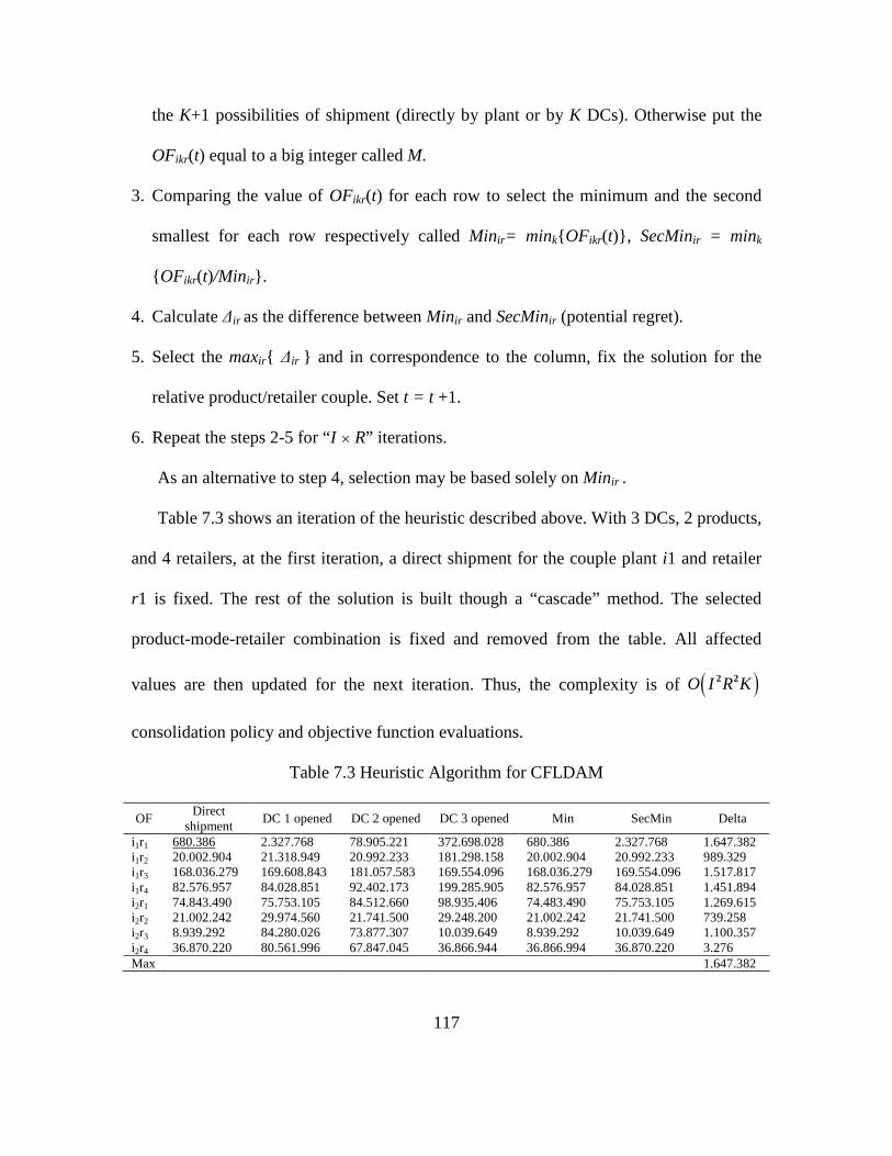
117

the K+1 possibilities of shipment (directly by plant or by K DCs). Otherwise put the

OFikr(t) equal to a big integer called M.

3. Comparing the value of OFikr(t) for each row to select the minimum and the second

smallest for each row respectively called Minir= mink{ OFikr(t)}, SecMinir = mink

{ OFikr(t)/Minir}.

4. Calculate ∆ir as the difference between Minir and SecMinir (potential regret).

5. Select the maxir{ ∆ir } and in correspondence to the column, fix the solution for the

relative product/retailer couple. Set t = t +1.

6. Repeat the steps 2-5 for “I × R” iterations.

As an alternative to step 4, selection may be based solely on Minir .

Table 7.3 shows an iteration of the heuristic described above. With 3 DCs, 2 products,

and 4 retailers, at the first iteration, a direct shipment for the couple plant i1 and retailer

r1 is fixed. The rest of the solution is built though a “cascade” method. The selected

product-mode-retailer combination is fixed and removed from the table. All affected

values are then updated for the next iteration. Thus, the complexity is of ( )2 2O I R K

consolidation policy and objective function evaluations.

Table 7.3 Heuristic Algorithm for CFLDAM

OF Direct

shipment DC 1 opened DC 2 opened DC 3 opened Min SecMin Delta

i1r1 680.386 2.327.768 78.905.221 372.698.028 680.386 2.327.768 1.647.382 i1r2 20.002.904 21.318.949 20.992.233 181.298.158 20.002.904 20.992.233 989.329 i1r3 168.036.279 169.608.843 181.057.583 169.554.096 168.036.279 169.554.096 1.517.817 i1r4 82.576.957 84.028.851 92.402.173 199.285.905 82.576.957 84.028.851 1.451.894 i2r1 74.843.490 75.753.105 84.512.660 98.935.406 74.483.490 75.753.105 1.269.615 i2r2 21.002.242 29.974.560 21.741.500 29.248.200 21.002.242 21.741.500 739.258 i2r3 8.939.292 84.280.026 73.877.307 10.039.649 8.939.292 10.039.649 1.100.357 i2r4 36.870.220 80.561.996 67.847.045 36.866.944 36.866.994 36.870.220 3.276 Max 1.647.382

118


To evaluate the performance of proposed heuristics, extensive computational experiments

are provided in this section.


Products are divided into two different product sets in the tests. Consolidation is allowed

for shipping products in the same product set, but products from different product sets

must be shipped separately. Holding costs for products are different for different product

sets and different holding places.

Production facilities and retailers are chosen as major cities in the United States.

Potential DCs can be located at the locations of retailers. Each DC has three possible

sizes: small, medium and large. The distances among cities are supplied by Daskin

(1995). The fixed cost of each DC is calculated on basis of home value in the respective

cities which is also supplied by Daskin (1995) and capacity of the DC which is set

according to potential service amount.

Demands of products at each retailer are normally distributed. The mean is

proportional to the population around that retailer. The variance of demand is calculated

using coefficient of variation times mean demand. Using trucks to distribute products,

lead time between two cities depends on the distance and speed of a truck (500

miles/day). Each truck has specified capacity. Shipping cost of one order is computed as

the fixed cost of using trucks plus variable costs which depends on distance and shipping

quantity.

119

Eight scenarios are compared defining the set of plants, possible sites for opening

DCs, customers’ locations and kind of function used to define the batch size. The eight

scenarios are shown in Table 7.4.

Table 7.4 Scenarios construction for CFLDAM

Scenario # Plants # Locations for DCs

#Customers Function to define the batch size

Length of Chromosome (genes)

1 2 10 10 Floor 140 2 2 10 10 Ceiling 140 3 5 10 10 Floor 600 4 5 10 10 Ceiling 600 5 2 10 49 Floor 608 6 2 10 49 Ceiling 608 7 5 10 49 Floor 2745 8 5 10 49 Ceiling 2745

Using the chromosome representation described in the Section 7.3, the length of

chromosome is defined as: Chromosome’s length = (number of plants× number of

customers) + (number of plants× number of possible sites for DCs) + (number of

possible sites for DCs× number of customers). The length of chromosome joined with the

number of iterations required to reach a feasible solution determines the complexity of

the algorithm and consequently the computation time (CPU). Each element of the

chromosome is called a gene so length is defined as number of genes.

The population size is equal to 100 individuals for the first 6 scenarios and equal to

10 for the last two scenarios. The number of iterations has been fixed equal to 50,000.

The GA stops when it fails to improve the solution for 10,000 continuous iterations.

120


For each scenario in Table 7.4, the performance of the genetic and the two versions of the

heuristic algorithms is tested and compared. In addition to the two heuristics discussed

earlier, the cost for all direct-shipping is also calculated. Table 7.5 presents the results

obtained for the scenarios presented in the previous section.

Table 7.5 Computational Results for CFLDAM

Genetic

Heuristic (Max {Delta = SecMin – Min})

Heuristic (Min {Min}) All Direct-shipping

CPU Time (sec)

No. Iter.

Objective Value

No. DCs

CPU Time (sec)

No. Iter.

Objective Value

No. DCs

CPU Time (sec)

No. Iter.

Objective Value

No. DCs

Objective Value

1 98 422 3.0567E+8 4 1 20 3.0303E+8 3 1 20 3.0303E+8 3 4.2113E+8

2 123 329 3.0551E+8 4 1 20 3.0302E+8 3 1 20 3.0303E+8 3 4.2112E+8

3 1435 9238 1.1807E+9 4 3 50 9.8272E+8 6 3 50 9.8462E+8 7 1.1800E+9 4 1203 1399 1.1797E+9 4 3 50 9.7914E+8 7 2 50 9.8462E+8 7 1.1801E+9 5 80 652 5.0602E+7 0 10 98 5.0602E+7 0 10 98 5.0602E+7 0 5.0602E+7

6 39 589 5.0618E+7 0 10 98 5.0618E+7 0 9 98 5.0618E+7 0 5.0618E+7

7 17771 23760 1.7430E+8 1 49 245 1.5454E+8 0 25 245 1.5452E+8 1 1.5454E+8

8 20486 25900 1.5152E+8 1 49 245 1.5452E+8 1 24 245 1.5452E+8 1 1.5454E+8

From all the experiment running results, the following observations are obtained:

1. The heuristic proved computationally efficient and provided the best solution in all

but one case (scenario 8).

2. The “delta” form of the heuristic (making the selection based on difference between

the best and second best options) outperformed the “min” form in two cases and the

“min” form performed best in one case.

3. As expected, both forms of the heuristic performed at least as well as direct shipments

in all cases and better in five of eight cases for the delta version and six of eight for

the min version.

121

4. The genetic algorithm found the unique best feasible solution in the last case and tied

for best in two additional cases where no DCs were opened. However the genetic

algorithm required significantly longer computation time.

Larger scenarios is also tested for examples containing a set of 88 customers, 2 or 5

plants, and 190 possible sites where opening DCs as suggested by Daskin. In these cases

the GA gives solutions in a reasonable time depending by the choice of population size.

These results are not reported here due to the difficulty to evaluate the goodness of these

solutions.

122

8. CONCLUSION AND FUTURE WORK

In this dissertation, an innovative framework for designing a multi-product integrated

supply chain network is proposed. I have derived and evaluated the effectiveness of a

two-phase solution methodology for solving this integrated location, inventory and

distribution problem. Transshipment is allowed between DCs to provide the functions of

both consolidation and distribution, and routing delivery strategy is considered for

delivering mixed-products from DCs to served retailers. A transshipment network is a

realistic representation of many real world problems that have a general network structure

with many supply/demand points and interconnecting links. While becoming more

complicated, it has immense applications in industry. Routing delivery strategy is also

generally used in industries to take the advantages of full truck load, especially when

served customers are close together and each individual demand is small compared to the

routing vehicle’s capacity.

A mixed-integer programming model is proposed for the full problem and sub-

problems in each phase. However, due to the complexity of the problem, several heuristic

methods are generated in each phase to find a good solution in a reasonable time.

In phase I, the multi-product FLP is solved subject to all the constraints in the original

model except that the routings are restricted to direct shipment by using estimated routing

cost parameters. The accuracy of the estimated routing cost parameters is discussed in

Chapter 6. A hybrid TS-SA method with an initial solution starting minimizing total IRC

is finally selected to solve the phase I model. The optimal solution to Phase I is always

feasible to the original problem and determines the locations of DCs and PWs/retailers

assignments.

123

Phase II model solves the routing problem for each opened DC and its assigned

retailers. The associated delivery problem is formulated as a capacitated IRP with

additional constraints to solve the optimal routing tours and frequencies simultaneously.

The study on this problem enriches the existing literature of IRP, and the proposed MS

method provides an alternative to solve complicated real life distribution problems with

heterogeneous fleet efficiently.

Computational performance of this proposed two-phase methodology is promising.

The heuristics are able to solve the problem within reasonable time frame for a broad

range of problem sizes and the solution from heuristics significantly improves the general

greedy solution.

There are several potential extensions from this work. First, even the proposed

heuristics can apply to the integrated problem where the number of PWs for each plant is

greater than one, only the special case of the original problem where only one PW is

allowed for each plant is discussed in detail in current research. Extra experiments could

be performed to discuss available heuristics.

Second, from an academic research point of view, new algorithms that can provide a

more accurate lower bound solution for the integrated problem, other than using the

CPLEX MIP solver to solve the model without nonlinear terms directly, will be of

interest. For a noticeable number of test cases experienced, the time required for CPLEX

even to verify the optimal solution to the model without nonlinear terms was excessive

(test results in Section 4.6).

Third, in this dissertation, DC locations and retailer assignments are determined and

then fixed in Phase I model, an algorithm allowing updating these decisions by

124

considering the routing information solved in Phase II could be of a great value to the real

world needs.

Finally, the usage of routing strategy is one important innovation in this dissertation

when deciding DC locations. As discussed in Chapter 6, the final routing structure highly

depends on the demand/retailer density, and extra research could be done to provide

better IRC estimation under different demand/retailer structures.

In addition, Chapter 7 presents an innovative model to guide the design of a

distribution network for shipping multiple products, each originating from its unique

production plant, to retailers considering different product consolidation sets. Shipments

may be direct or use intermediate DCs for shipment consolidation and/or inventory

pooling prior to final delivery to retail demand points. Facility costs, inventory costs and

shipping costs are considered. This model is flexible and may consider factors such as

multiple types of delivery trucks for each segment, full or less than full truck shipments

and different service requirements. A bound is derived on the maximum cost penalty that

could be incurred from restricting all deliveries to full truck loads.

Two versions of a greedy construction heuristic and a genetic algorithm are

developed to solve the model. The construction heuristics are shown to provide

computationally efficient approaches to obtain good solutions as compared to a direct

shipment strategy. Given a set of possible DC locations and standard cost data for

shipping alternatives and storage, the user can evaluate one or multiple scenarios and

generate a system design by applying the heuristic. The genetic algorithm also provides

good, feasible solutions but requires greater computational effort to produce comparable

results.

125

In this work, I assume a continuous demand distribution, experimentation further

assumed a Gaussian distribution. Future work could explore discrete demand. Another

possible improvement can be the consideration of an additional level of consolidation that

would allow for early consolidation from multiple plants for long shipments to demand

regions which are then divided into delivery orders at local DCs within demand regions.

With regards to model solution, other chromosome definitions may be considered for the

genetic algorithm. The use of integers instead of binary values could improve the running

time as a result of chromosome’s length reduction. Sensitivity to shipping policies could

able be investigated.

126

REFERENCE

Ai, T. J., & Kachitvichyanukul, V. (2009). A particle swarm optimization for the vehicle routing problem with simultaneous pickup and delivery. Computers & Operations Research, 36, 1693-1702.

Albareda-Sambola, M., Fernández, E., Hinojosa, Y., & Puerto, J. (2009). The multi-period incremental service facility location problem. Computers & Operations Research, 36, 1356-1375.

Anily, S., & Bramel, J. (2004). An asymptotic 98.5%-effective lower bound on fixed partition policies for the inventory-routing problem. Discrete Applied Mathematics, 145, 22-39.

Archetti, C., Bertazzi, L., Laporte, G., & Speranza, M. G. (2007). A branch-and-cut algorithm for a vendor-managed inventory-routing problem. Transportation Science, 41, 382-391.

Askin, R. G., Baffo, I., & Xia, M. (2010). Multi-commodity warehouse location and distribution planning with inventory consideration. International Journal of Production Research, In process. https://docs.google.com/viewer?a=v&pid=sites&srcid=ZGVmYXVsdGRvbWFpbnxtaW5nanVueGlhfGd4OjNiNzM0MDk1YTYxNGUzYjU Askin, R. G., & Xia, M. (2012). Hybrid heuristics for infinite period inventory routing problem. In Michael, K.O. (Ed.), Progress in 12th International Material Handling Research Colloquium. https://docs.google.com/viewer?a=v&pid=sites&srcid=ZGVmYXVsdGRvbWFpbnxtaW5nanVueGlhfGd4Ojc5ZjcyZjUxYTMxNDYxODY

Averbakh, I., Berman, O., Drezner, Z., & Wesolowsky, G. O. (2007). The uncapacitated facility location problem with demand-dependent setup and service costs and customer-choice allocation. European Journal of Operational Research, 179, 956-967.

Ballou, R. H. (2003). Business Logistics: Supply Chain Management. (5th ed.). Prentice Hall.

Ballou, R. H. (1968). Dynamic warehouse location analysis. Journal of Marketing Research, 5, 271-276.

Bard, J. F., & Nananukul, N. (2010). A branch-and-price algorithm for an integrated production and inventory routing problem. Computers & Operations Research, 37, 2202-2217.

127

Berbeglia, G., Pesant, G., & Rousseau, L. (2012). Feasibility of the pickup and delivery problem with fixed partial routes: a complexity analysis. Transportation Science, 46, 359-373.

Berger, J., & Barkaoui, M. (2004). A parallel hybrid genetic algorithm for the vehicle routing problem with time windows. Computers & Operations Research, 31, 2037-2053.

Bertazzi, L., Paletta, G., & Speranza, M. G. (2002). Deterministic order-up-to level policies in an inventory routing problem. Transportation Science, 36, 119-132.

Bertazzi, L., Savelsbergh, M., & Speranza, M. G. (2008). Inventory routing. in anonymous the vehicle routing problem, 49-72.

Bidhandi, H. M., & Yusuff, R. M. (2011). Integrated supply chain planning under uncertainty using an improved stochastic approach. Applied Mathematical Modelling, 35, 2618-2630.

Chan, Y., Carter, W. B., & Burnes, M. D. (2001). A multiple-depot, multiple-vehicle, location-routing problem with stochastically processed demands. Computers & Operations Research, 28, 803-826.

Chaudhry, S.S., He, S.S., & Chaudhry, P.E. (2003). Solving a class of facility location problems using genetic algorithms. Expert System, 20, 86-91.

Clark, A. J., & Scarf, H. (1960). Optimal policies for a multi-echelon inventory problem. Management Science, 6, 475-490.

Cornejols, R., Sridharan, R., & Thizy, J. M. (1991). A comparison of heuristics and relaxations for the capacitated plant location problem. European Journal of Operational Research, 50, 280-297.

Daskin, M.S., Collard, C. R., & Shen, Z. M. (2002). An inventory-location model: formulation, solution algorithm and computational results. Annals of Operations Research, 110, 83-106.

Daskin, M.S. (1995). Network and Discrete Location-Models, Algorithms, and Applications, Wiley-Interscience Series in Discrete Mathematics and Optimization.

Desrochers, M., & Laporte, G. (1991). Improvements and extensions to the Miller–Tucker–Zemlin subtour elimination constraints. Operations Research Letters, 10, 27–36.

Dror, M., & Ball, M. (1987). Inventory/Routing: reduction from an annual to a short-period problem. Naval Research Logistics Quarterly, 34, 891-905.

128

Dror, M., Ball, M., & Golden, B. (1985). A computational comparison of algorithms for the inventory routing problem. Annals of Operations Research, 4, 3-23.

Efroymson, M.A., & Ray, T.L. (1966). A branch and bound algorithm for plant location. Operations Research, 14, 361-368.

Elhedhli, S., & Gzara, F. (2008). Integrated design of supply chain networks with three echelons, multiple commodities and technology selection. IIE Transactions, 40, 31-44.

Erlebacher, S. J., & Meller, R. D. (2000). The interaction of location and inventory in designing distribution systems. IIE Transactions, 32, 155-166.

Ertogral, K., Darwish, M., & Ben-Day, M. (2007). Production and shipment lot sizing in a vendor-buyer supply chain with transportation cost. European Journal of Operational Research, 176, 1592-1606.

Federgruen, A., & Zipkin, P. (1984). A combined vehicle routing and inventory allocation problem. Operations Research, 32, 1019-1032.

Fisher, M. L. (1995). Network Routing, Handbooks in Operations Research and Management Science. Elsevier Science.

Franke, P.D., (2010). Vendor-managed inventory for high value parts: results from a survey among leading international manufacturing firms. Berlin: Berlin Institute of Technology.

Gebennini, E., Gamberini, R., & Manzini, R. (2009). An integrated production–distribution model for the dynamic location and allocation problem with safety stock optimization. International Journal of Production Economics, 122, 286-304.

Golden, B., Assad, A., & Dahl, R. (1984). Analysis of a large scale vehicle routing problem with an inventory component. Large Scale Systems, 7, 181-190.

Golden, B. L. (1988). Vehicle Routing: Methods and Studies. North-Holland.

Gutiérrez-Jarpa, G., Desaulniers, G., Laporte, G., & Marianov, V. (2010). A branch-and-price algorithm for the vehicle routing problem with deliveries, selective pickups and time windows. European Journal of Operational Research, 206, 341-349.

Haimovich, M., & Rinnooy Kan, A. H. G. (1985). Bounds and heuristics for capacitated routing problems. Mathematics of Operations Research, 10, 527-542.

Hall, R. W. (1985). Determining vehicle dispatch frequency when shipping frequency differs among suppliers. Transportation Research B, 19, 421-431.

129

Harkness, J., & ReVelle, C. (2003). Facility location with increasing production costs. European Journal of Operational Research, 145, 1-13.

Harland, C. M. (1996). Supply Chain Management, Purchasing and Supply Management, Logistics, Vertical Integration, Materials Management and Supply Chain Dynamics, Blackwell Encyclopedic Dictionary of Operations Management. Blackwell: U.K.

Hinojosa, Y., Puerto, J., & Fernández, F. R. (2000). A multi-period two-echelon multi-commodity capacitated plant location problem. European Journal of Operational Research, 123, 271-291.

Ho, W., Ho, G. T. S., Ji, P., & Lau, H. C. W. (2008). A hybrid genetic algorithm for the multi-depot vehicle routing problem. Engineering Applications of Artificial Intelligence, 21, 548-557.

Hoff, A., Gribkovskaia, I., Laporte, G., & Løkketangen, A. (2009). Lasso solution strategies for the vehicle routing problem with pickups and deliveries. European Journal of Operational Research, 192, 755-766.

Holmberg, K., Ronnqvist, M., & Yuan, D. (1999). An exact algorithm for the capacitated facility location problems with single sourcing. European Journal of Operational Research, 113, 544-559.

Hosage, C.M., & Goodchild, M.F. (1986). Discrete space location-allocation solutions for genetic algorithms. Annals of Operations Research, 6, 35-46.

Huang, S., & Lin, P. (2010). A modified ant colony optimization algorithm for multi-item inventory routing problems with demand uncertainty. Transportation Research Part E, 46, 598-611.

Jamarillo, J.H., Bhadury, J., & Batta, R. (2002). On the use of genetic algorithm to solve location problems. Computers & Operations Research, 29, 761-779.

Javid, A. A., & Azad, N. (2010). Incorporating location, routing and inventory decisions in supply chain network design. Transportation Research Part E, 46, 582-597.

Laporte, G. (2009). Fifty years of vehicle routing. Transportation Science, 43, 408-416.

Lee, B. K., Kang, K. H., & Lee, Y. H. (2008). Decomposition heuristic to minimize total cost in a multi-level supply chain network. Computers & Industrial Engineering, 54, 945-959.

130

Li, J., Chen, H., & Chu, F. (2010). Performance evaluation of distribution strategies for the inventory routing problem. European Journal of Operational Research, 202, 412-419.

Li, J., Chu, F., & Chen, H. (2011). A solution approach to the inventory routing problem in a three-level distribution system. European Journal of Operational Research, 210, 736-744.

Li, X. (2010). Optimal inventory policies in decentralized supply chains. International Journal of Production Economics, 128, 303-309.

Lin, S., Lee, Z., Ying, K., & Lee, C. (2009). Applying hybrid meta-heuristics for capacitated vehicle routing problem. Expert Systems with Applications, 36, 1505-1512.

Liu, K., Zhou, Y., & Zhang, Z. (2010). Capacitated location model with online demand pooling in a multi-channel supply chain. European Journal of Operational Research, 207, 218-231.

Marinakis, Y., Marinaki, M., & Dounias, G. (2010). A hybrid particle swarm optimization algorithm for the vehicle routing problem. Engineering Applications of Artificial Intelligence, 23, 463-472.

Mazzola, J. B., & Neebe, A. W. (1999). Lagrangian-relaxation-based solution procedures for a multiproduct capacitated facility location problem with choice of facility type. European Journal of Operational Research, 115, 285-299.

Melo, M. T., Nickel, S., & Saldanha-da-Gama, F. (2012). A tabu search heuristic for redesigning a multi-echelon supply chain network over a planning horizon. International Journal of Production Economics, 136, 218-230.

Melo, M. T., Nickel, S., & Saldanha-da-Gama, F. (2005). Dynamic multi-commodity capacitated facility location: a mathematical modeling framework for strategic supply chain planning. Computers & Operations Research, 33, 181-208.

Min, H., Jayaraman, V., & Srivastava, R. (1998). Combined location-routing problems: A synthesis and future research directions. European Journal of Operational Research, 108, 1-15.

Miranda, P., & Garrido, R. A. (2009). Inventory service-level optimization within distribution network design problem. International Journal of Production Economics, 122, 276-285.

131

Miranda, P. A., & Garrido, R. A. (2008). Valid inequalities for lagrangian relaxation in an inventory location problem with stochastic capacity. Transportation Research Part E, 44, 47-65.

Miranda, P. A., & Garrido, R. A. (2004). Incorporating inventory control decisions into a strategic distribution network design model with stochastic demand. Transportation Research Part E, 40, 183-207.

Moin, N. H., Salhi, S., & Aziz, N. A. B. (2011). An efficient hybrid genetic algorithm for the multi-product multi-period inventory routing problem. International Journal of Production Economics, 133, 334-343.

Nagy, G., & Salhi, S. (2007). Location-routing: Issues, models and methods. European Journal of Operational Research, 177, 649-672.

Nagy, G., & Salhi, S. (2005). Heuristic algorithms for single and multiple depot vehicle routing problems with pickups and deliveries. European Journal of Operational Research, 162, 126-141.

Nenes, G., Panagiotidou, S., & Tagaras, G. (2010). Inventory management of multiple items with irregular demand: A case study. European Journal of Operational Research, 205, 313-324.

Nozick, L. K., & Turnquist, M. A. (2001). Inventory, transportation, service quality and the location of DCs. European Journal of Operational Research, 129, 362-371.

Ozsen, L., Coullard, C. R., & Daskin, M. S. (2008). Capacitated warehouse location model with risk pooling. Naval Research Logistics, 55, 295-312.

Park, S., Lee, T., & Sung, C. S. (2010). A three-level supply chain network design model with risk-pooling and lead times. Transportation Research Part E, 46, 563-581.

Pirkul, H., & Jayaraman, V. (1998). A multi-commodity, multi-plant, capacitated facility location problem: formulation and efficient heuristic solution. Computers Operations Research, 25, 869-878.

Pillac, V., Gendreau, M., Guéret, C., & Medaglia, A. L. (2012) A review of dynamic vehicle routing problems. European Journal of Operational Research, Accepted manuscript, doi:10.1016/j.ejor.2012.08.015.

Pourakbar, M., Farahani, R. Z., & Asgari, N. (2007). A joint economic lot-size model for an integrated supply network using genetic algorithm. Applied Mathematics and Computation, 189, 583-596.

132

Qi, L., & Shen, Z. M. (2007). A supply chain design model with unreliable supply. Naval Research Logistics, 54, 829-844.

Roundy, R. (1986). A 98% effective lot-sizing rule for a multi-product multi-state production inventory system. Mathematics of Operations Research, 11, 699-727.

Santoso, T., Ahmed, S., Goetschalckx, M., & Shapiro, A. (2005). A stochastic programming approach for supply chain network design under uncertainty. European Journal of Operational Research, 167, 96-115.

Schmitt, A. J., Snyder, L. V., & Shen, Z. M. (2010). Inventory systems with stochastic demand and supply: Properties and approximations. European Journal of Operational Research, 206, 313-328.

Shen, S., & Honda, M. (2009). Incorporating lateral transfers of vehicles and inventory into an integrated replenishment and routing plan for a three-echelon supply chain. Computers & Industrial Engineering, 754, 775.

Shen, Z. M., & Daskin, M. S. (2005). Trade-offs between customer service and cost in integrated supply chain design. Manufacturing & Service Operations Management, 7, 188-207.

Shen, Z.M. and Qi, L., (2007). Incorporating inventory and routing costs in strategic location models. European Journal of Operational Research 179, 372-389.

Shu, J., Chung-Piaw Teo, C., & Shen, Z. M. (2005). Stochastic transportation-inventory network design problem. Operations Research, 53, 48-60.

Silver, E. A., Pyke, D. F., & Peterson, R. (1998). Inventory Management and Production Planning and Scheduling. (3rd ed.). Wiley: New York.

Snyder, L. V., & Daskin, M. (2005). Reliability models for facility location: the expected failure cost case. Transportation Sience, 39, 400-416.

Solyalı, O., Cordeau, J., & Laporte, G. (2012). Robust inventory routing under demand uncertainty. Transportation Science, 46, 327-340.

Sourirajan, K., Ozsen, L., & Uzsoy, R. (2009). A genetic algorithm for a single product network design model with lead time and safety stock considerations. European Journal of Operational Research, 197, 599-608.

Sourirajan, L., Ozsen, L., & Uzsoy, R. (2009). A single product network design model with lead time and safety stock considerations. IIE Transactions, 39, 411-424.

133

Subramanian, A., Drummonda, L. M. A., Bentes, C., Ochi, L. S., & Farias, R. (2010). A parallel heuristic for the Vehicle Routing Problem with Simultaneous Pickup and Delivery. Computers & Operations Research, 37, 1899-1911.

Tagaras, G., & Vlachos., D. (2001). A periodic review inventory system with emergency replenishments. Management Science, 47, 415-429.

Toth, P., & Tramontani, A. (2008). An integer linear programming local search for capacitated vehicle routing problems. in anonymous The Vehicle Routing Problem (pp. 275-295).

Uday Apte, M. & Viswanathan, S. (2000) Effective cross docking for improving distribution efficiencies. International Journal of Logistics: Research and Applications, 3, 291–302.

Waller, M. A., Cassady, C. R., & Ozment, J. (2006). Impact of cross-docking on inventory in a decentralized retail supply chain. Transportation Research Part E, 42, 359-382.

Weber, A. (1909 (translated by Friedrich, C.J)). Theory of the Location of Industries. The University of Chicago Press: Chicago.

Xia, M, & Askin, R.G.. (2012). Multi-product supply chain network design with location, inventory and routing decisions. In process. https://docs.google.com/viewer?a=v&pid=sites&srcid=ZGVmYXVsdGRvbWFpbnxtaW5nanVueGlhfGd4OmMyMDM2MTc0YTBjMTFhMg

Yao, Z., Lee, L. H., Jaruphongsa, W., Tan, V., & Hui, C. F. (2010). Multi-source facility location–allocation and inventory problem. European Journal of Operational Research, 207, 750-762.

Yu, Y., Chen, H., & Chu, F. (2008). A new model and hybrid approach for large scale inventory routing problems. European Journal of Operational Research, 189, 1022-1040.

Yurtkuran, A., & Emel, E. (2010). A new hybrid electromagnetism-like algorithm for capacitated vehicle routing problems. Expert Systems with Applications, 37, 3427-3433.

Zachariadis, E. E., Tarantilis, C. D., & Kiranoudis, C. T. (2009). An integrated local search method for inventory and routing decisions. Expert Systems with Applications, 36, 10239-10248.

Zhao, Q., Chen, S., & Zang, C. (2008). Model and algorithm for inventory/routing decision in a three-echelon logistics system. European Journal of Operational Research, 191, 623-635.

134

Zhou G., Min H., & Gen M. (2003) A genetic algorithm approach to the bi-criteria allocation of customers to warehouses. International Journal of Production Economics, 86, 35-45.

Zipkin, P. H. (2000). Foundations of Inventory Management. (1st ed.). McGraw-Hill: New York.

135

APPENDIX A

OPTIMAL FREQUENCY

136

Minimize: 0.5 1

( )v

vrv v r rr S

v v

dy a cd h z

pα

µγ σ

γ γ∈

= + + + +

∑

Let: 0.5

0.5

/

v

v

v

v

r rr S

r rr S

v

x

A a cd

B h

C h z

D d p

α

γ

µ

σ

∈

∈

=

= +

=

=

=

∑∑

Then the objective function becomes: 1B

y Ax C Dx x

= + + +

where A, B, C, and D are positive constants, x is an independent positive variable. The

problem is to find the value of x to minimize y.

2 2

22

1 1

2 1

1

2

0

dy B CA

dx x xD

xB C

Ax

x Dx

= − + −

+

= − −

+

=

3/2 1/22

2 3 2 2 3

3/2334

3/234

2 1 1 1 1

2 2

2

114

14

2

14

>0

d y B C CD D

dx x x x x x x

B C C

xx Dx D

xx

C Cx DB x

xx D

x

− − = − − + − + + −

= − − ++

− + += +

+

137

APPENDIX B

UPPER BOUND ON THE LOSS FROM USE OF FULL TRUCK LOAD

138

The proposed model in Chapter 7 assumes use of full-truck loads in transportation.

However, the number of full-trucks in each order may be greater than 1. In practice, these

loads may be staggered but this research assumes that all are shipped jointly in current

inventory calculations. The model could be readily adjusted for other shipping scenarios

as discussed earlier in the paper. An upper bound on the loss from use of full truck load

shipments is derived here.

For each supplier-customer pair, the total cost for this pair given a policy needs to be

minimized. Using the same parameters as in the paper:

Minimize ( )2

Q D QTC A a bl Q h

C Q = + ⋅ + ⋅ ⋅ + ⋅

(B-1)

Let the optimal quantityQ mC= , where m may not be an integer. Total Cost function

(B-1) becomes

( ) ( )2

D m CTC m A a m bl m C h

m C

⋅= + ⋅ + ⋅ ⋅ ⋅ + ⋅ ⋅

(B-2)

To know the maximum loss between this Q and the better of the floor and ceiling

function multiples of C, define:

1 2,m m m m= = ,

( ) ( )( )

1 2

2

min{ ( ); ( )}, 1

( ), 0 1

0, 1

TC m TC m TC m TC m if m

TC m TC m if m

if m

δ

− − >

= − < < =

( ) 11 1

1 1

1 1( ) ( ) ( ) ( )

2

m mAD aD hCTC m TC m m m

C m m C m m

− = − + − + −

Note that 11m m m− ≤ ≤

139

( )

( )

1

1

1 1( ) ( ) (1 ) ( )

1 2

( )( 1)

mAD aD hCTC m TC m m m

C m m C mAD

TC m TC mCm m

∴ − ≤ − + − + −−

∴ − ≤−

( ) 22 2

2 2

1 1( ) ( ) ( ) ( )

2

m mAD aD hCTC m TC m m m

C m m C m m

− = − + − + −

Note that 2 1m m m≤ ≤ +

( )

( )

2

2

1 1( ) ( ) (1 ) ( 1 )

1 2

( )2

mAD aD hCTC m TC m m m

C m m C mhC

TC m TC m

∴ − ≤ − + − + + −+

∴ − ≤

min{ ; }, 1( 1) 2

, 0 12

0, 1

AD hCif m

Cm m

hCif m

if m

δ

> −∴ ≤

< <

=

In conclusion, 2

hCδ ≤

Integrated Supply Chain Network Design: Location ... Supply Chain Network Design: Location,...

Documents

Transcript of Integrated Supply Chain Network Design: Location ... Supply Chain Network Design: Location,...