Integrated Flight Dynamics and

Aeroelasticity of Flexible Aircraft with

Application to Swept Flying Wings

Robert J. S. Simpson∗ and Rafael Palacios†,

Imperial College, London, SW7 2AZ, United Kingdom

The dynamics of flexible, swept flying wing (SFW) aircraft are described by a set of

nonlinear, multi-disciplinary equations of motion. Aircraft structures are modeled us-

ing a geometrically-exact composite beam model which can, in general, capture large

dynamic deformations and the interaction between rigid-body and elastic degrees-of-

freedom. In addition, an implementation of the unsteady vortex-lattice method capa-

ble of handling arbitrary kinematics is used to capture the unsteady, three-dimensional

flow-field around the aircraft as it deforms. Linearization of this coupled nonlinear

description, which can in general be around a nonlinear equilibrium, is performed

to yield linear time-invariant state-space models. Verification of aeroelastic stability

analyses using these models is carried out. Subsequently, a set of SFW models are

developed and the dynamic stability characteristics of these aircraft are investigated

for a range of flight velocities and vehicle parameters.

Nomenclature

A state-space system matrix / sectional area, m2

A aerodynamic influence coefficient matrix (downwash)

AU aerodynamic influence coefficient matrix (velocity)

B state-space input matrix

C constant sparse matrix / state-space output matrix

C tangent damping matrix

∗Graduate Student, Department of Aeronautics, 363A Roderic Hill Building; r.simpson11@imperial.ac.uk.AIAA Student Member.†Reader, Department of Aeronautics, 355 Roderic Hill Building; r.palacios@imperial.ac.uk. AIAA Mem-

ber.

1 of 17

E Young’s modulus

f frequency, Hz

G shear modulus

I moment of inertia, kg·m2

J sectional polar 2nd moment of area, m4

K tangent stiffness

k discrete time step index

m mass, kg

Q generalized nodal forces

q dynamic pressure, Pa

∆t discrete time step, s

Uext External fluid velocities, m·s−1

u system inputs

v velocity of body-fixed frame, m·s−1

w downwash at collocation points, m·s−1

x system states

β rigid-body degrees-of-freedom

Γ circulation, m2·s−1

η structural degrees of freedom

Θ Euler angles, rad

ζ aerodynamic grid coordinates

ρ∞ free-stream air density, kg·m−3

χ quaternions

ω angular velocity vector of body-fixed frame, rad·s−1

Subscript

(•)0 reference condition

(•)g pertaining to gust inputs

(•)∞ free-stream quantity

(•)f flutter condition

Superscript

F fluid degrees-of-freedom

R rigid-body degrees-of-freedom

S structural degrees-of-freedom

(•) time derivative

(•) linearized quantity / per unit beam length

(•)? pertaining to the wake

2 of 17

I. Introduction

The trend for ever more lightweight, slender aero-structures is pushing the design of next-

generation aircraft towards unprecedented levels of flexibility. A consequence of this is that

active aeroelastic control will be employed more often for stability augmentation and gust-

load alleviation, and is likely to be an enabling technology for future designs. This has forced

engineers to develop multi-disciplinary computational tools for early-stage and control system

design that can predict the interaction of aircraft elastic response, rigid-body motion, and

aerodynamic forcing.1,2, 3, 4, 5, 6 In addition to this, several flight test programs7,8 have been

developed recently that specifically target the phenomenon of aeroelastic/rigid-body coupling

with the intention of developing active aeroelastic control systems for stability augmentation

and disturbance rejection. Most saliently, the intended handover of the Lockheed-developed

X-56 Multi-Utility Technology Testbed (MUTT) to NASA has created a focal point for

public domain research into flexible aircraft flight dynamics (FAFD) and control.8,9, 10

As such, the goals of this work are to present a relatively simple test case, referred to

as the Swept Flying Wing (SFW), useful for investigating the control problems associated

with platforms similar to the X-56 test aircraft. Firstly, the analysis methodology used in

this work is described in Section II. Following this, verification of the static and dynamic

aeroelastic analyses are presented in Section III. Finally, the development of the SFW test

case is presented with stability analysis of the unconstrained aeroelastic response of the

aircraft in Section IV. In the future it is hoped that this computational model will be useful

for demonstrating active aeroelastic control technologies for stabilization and disturbance

rejection during simulations of the aircraft dynamics.

II. Methodology

In this section we present a flexible aircraft flight dynamics model based on coupling a

nonlinear composite beam model with the unsteady vortex-lattice method (UVLM). Follow-

ing this we present a linearization of the coupled model, and the re-casting of its underlying

equations into state-space form. These methods are the basis for the software implemen-

tation used in this work, referred to as Simulation of High-Aspect-Ratio Planes in Python

(SHARPy).

II.A. Nonlinear Flexible Aircraft Dynamics

A geometrically-exact composite beam model based on the formulations by Hodges11 and

Geradin & Cardona12 is used to capture the dynamics of flexible, unconstrained structures

subject to large (geometrically-nonlinear) deformations and nonlinear rigid-body motion.

3 of 17

A moving body-fixed reference system is used to track elastic deformations and rigid-body

motion of the structure. The resulting equations of motion (EoM) that describe a moving

flexible body are13

M (η)

ηβ+Qgyr (η, η, β) +Qstif (η) = Qext (η, η, β, χ) , (1)

where the structural degrees of freedom, η, are given in terms of nodal displacements and

finite rotations (parameterized using the Cartesian rotation vector)12 in a 2-noded finite-

element beam discretization. The rigid-body states, β, include the translational and angular

velocities of the origin of the body-fixed reference frame. These are denoted va and ωa

respectively. The system dynamics are coupled through the tangent mass matrix, M(η),

and the discrete gyroscopic and external forces, Qgyr and Qext, respectively. Computation

of the discrete elastic forces, Qstif , depend upon the elastic degrees-of-freedom, η. The

structural and rigid-body components (denoted by superscripts S and R, respectively) of

the gyroscopic, elastic and external forces can be identified as

Qgyr =

QSgyr

QRgyr

, Qstif =

QSstif

0

, and Qext =

QSext

QRext

(2)

respectively. A detailed description of the various terms in Eq. (1) can be found in previous

work by one of the authors.13 Finally, the orientation of the body-fixed reference frame with

respect to an inertial frame is parameterized using quaternions, denoted by χ, and computed

by solving an extra set of attitude EoM.14,15 Together with the Eq. (1) this completes the

geometrically nonlinear description of the aircraft structural dynamics and nonlinear rigid-

body motion.

Assuming coincident spanwise discretizations, an aerodynamic lattice ζ is constructed

that represents the aircraft lifting surfaces. From this discretization, the 3-D, geometrically-

nonlinear, unsteady aerodynamic loading is obtained using the unsteady vortex-lattice method.

In the UVLM, quadrilateral vortex ring elements are used to discretize both lifting surfaces

and their wakes. Each surface (bound) vortex ring has an associated circulation strength, Γ,

and a collocation point at which the non-penetration boundary condition is satisfied. The

Kutta condition and Joukowski hypothesis16 are approximately satisfied by shedding wake

vortex rings from the trailing-edge of each surface at every time step. A first-order, explicit

time-stepping scheme is employed.4,17,18 This results in a time-varying, discrete-time system

4 of 17

of equations, written for time step k + 1, of the form

A(ζ)Γk+1

+A?(ζ, ζ?)Γ?k+1

+ wk+1

= 0, (3)

Γ?k+1

= CΓΓk

+ C?ΓΓ?

k

, (4)

ζ?k+1 − Cζζ

k+1

= C?ζ ζ

?k + ∆t(AUΓ

k

+A?UΓ?k)

+ ∆tU?k

ext , (5)

where Eq.(3) enforces the non-penetration boundary condition on the aircraft geometry, and

Eqs. (4) & (5) propagate the wake circulation strength and wake geometry, respectively,

through time. Note that the ( )? superscript denotes an entity corresponding to the aircraft

wake, for example the lattice geometry of the free shear-layer, ζ?, or the corresponding vortex

ring strengths, Γ?. A more detailed description of the terms in (3) - (5) can be found in

previous work by the authors.19

The circulation distribution on the deformed aircraft is then post-processed to obtain the

aerodynamic loading which is then mapped back onto the structural nodes. Thus the flexible-

body dynamics and aerodynamics models are coupled to form a nonlinear aeroelastic model

of the dynamics of flexible aircraft. In the presence of geometrically nonlinear deformations

and complex kinematics all components of the aerodynamic forces must be captured when

post-processing the aircraft states to obtain aerodynamic load distributions.20,21

II.B. Linearization

The structural dynamics are linearized around reference condition (η0, η0, β0, χ0) and small

changes from this state are represented with over-bars, that is, (η, ˙η, β, χ). The linearized

(incremental) form of Eq. (1) around the reference state has the form13

M(η0)

¨η

˙β

+ C(η0, η0, β0)

˙η

β

+K(η0, η0, β0)

η0 = Qext

(η, ˙η, β, Θ

), (6)

where the constant tangent damping and stiffness matrices C and K, respectively, are ob-

tained through direct linearization of the discretized forces in Eq. (1). Note that Euler

angles, Θ, are preferred in the linear analysis to describe variations of the aircraft orienta-

tion.22 Projection of the linear EoM on the vibration modes of the unconstrained aircraft can

further simplify the structural representation of the vehicle dynamics. This linear, second-

order set of ODEs is then discretized in time using the Newmark-β scheme and cast in

state-space form and coupled with a linearized UVLM aerodynamics model.

A linearized form of the aerodynamics model is constructed using the model developed by

Murua et al.23 and based on the description by Hall.24 To obtain the state-space form of the

UVLM, the governing equations are linearized on a frozen aerodynamic geometry around the

5 of 17

aircraft trim condition, which may include large wing deformations and a non-planar wake.

Therefore, the system of Eqs. (3)-(5) is reduced to

A(ζ0)Γk+1

+A?(ζ0, ζ?0 )Γ?

n+1

+ wk+1

= 0, (7)

Γ?k+1

= CΓΓk

+ C?ΓΓ?

k

, (8)

where the over-bars again represent increments on the states about which the aircraft is

linearized. The aerodynamic equations above are coupled with the linear structural Eqs. (6)

and cast in the discrete-time state-space form

x(k + 1) = Ax(k) +Bu(k) +Bgug(k),

y(k) = Cx(k),(9)

where u are the actuator inputs and subscript-g terms correspond to gust inputs. The state

vector that completely determines the linear system is

x := (xF ; xS; xR) , (10)

where

xF := (Γ; Γ?; ˙Γ), (11)

xS := (η; ˙η) , (12)

xR :=(β; Θ

)(13)

Note that the time-rate-of-change of the bound vortex ring strengths, ˙Γ, is included in the

state vector as it is required for the computation of unsteady aerodynamic loads.23 This set

of coupled, linear EoM now form a suitable basis for stability analyses, model reduction, and

control syntheses.

III. Verification of aeroelastic analyses

Divergence and flutter of swept wings was investigated numerically and experimentally by

Ricketts and Doggett.25 In their experiments wind-tunnel models of forward-swept, isotropic,

cantilever wings (with the structure being a flat plate) were subjected to a range of dynamic

pressures, in some cases up to their divergence dynamic pressure, qD. For some of the

wing models flutter occurred prior to the onset of divergence - this was also reported and

predicted numerically in their work. The wing models are described in the planform sketches

of Figure 1 and structural properties of Table 1. This set of tests allows a benchmarking of

6 of 17

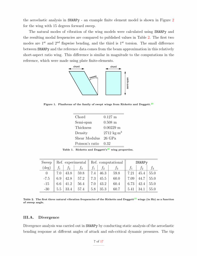
the aeroelastic analysis in SHARPy - an example finite element model is shown in Figure 2

for the wing with 15 degrees forward sweep.

The natural modes of vibration of the wing models were calculated using SHARPy and

the resulting modal frequencies are compared to published values in Table 2. The first two

modes are 1st and 2nd flapwise bending, and the third is 1st torsion. The small difference

between SHARPy and the reference data comes from the beam approximation in this relatively

short-aspect ratio wing. This difference is similar in magnitude to the computations in the

reference, which were made using plate finite-elements.

Figure 1. Planforms of the family of swept wings from Ricketts and Doggett.25

Chord 0.127 m

Semi-span 0.508 m

Thickness 0.00229 m

Density 2712 kg·m3

Shear Modulus 26 GPa

Poisson’s ratio 0.32

Table 1. Ricketts and Doggett’s25 wing properties.

Sweep Ref. experimental Ref. computational SHARPy

(deg) f1 f2 f3 f1 f2 f3 f1 f2 f3

0 7.0 43.8 59.8 7.4 46.3 59.8 7.21 45.4 55.0

-7.5 6.9 42.8 57.2 7.3 45.5 60.0 7.09 44.7 55.0

-15 6.6 41.2 56.4 7.0 43.2 60.4 6.73 42.4 55.0

-30 5.5 33.4 57.4 5.8 35.3 60.7 5.41 34.1 55.0

Table 2. The first three natural vibration frequencies of the Ricketts and Doggett25 wings (in Hz) as a functionof sweep angle.

III.A. Divergence

Divergence analysis was carried out in SHARPy by conducting static analysis of the aeroelastic

bending response at different angles of attack and sub-critical dynamic pressures. The tip

7 of 17

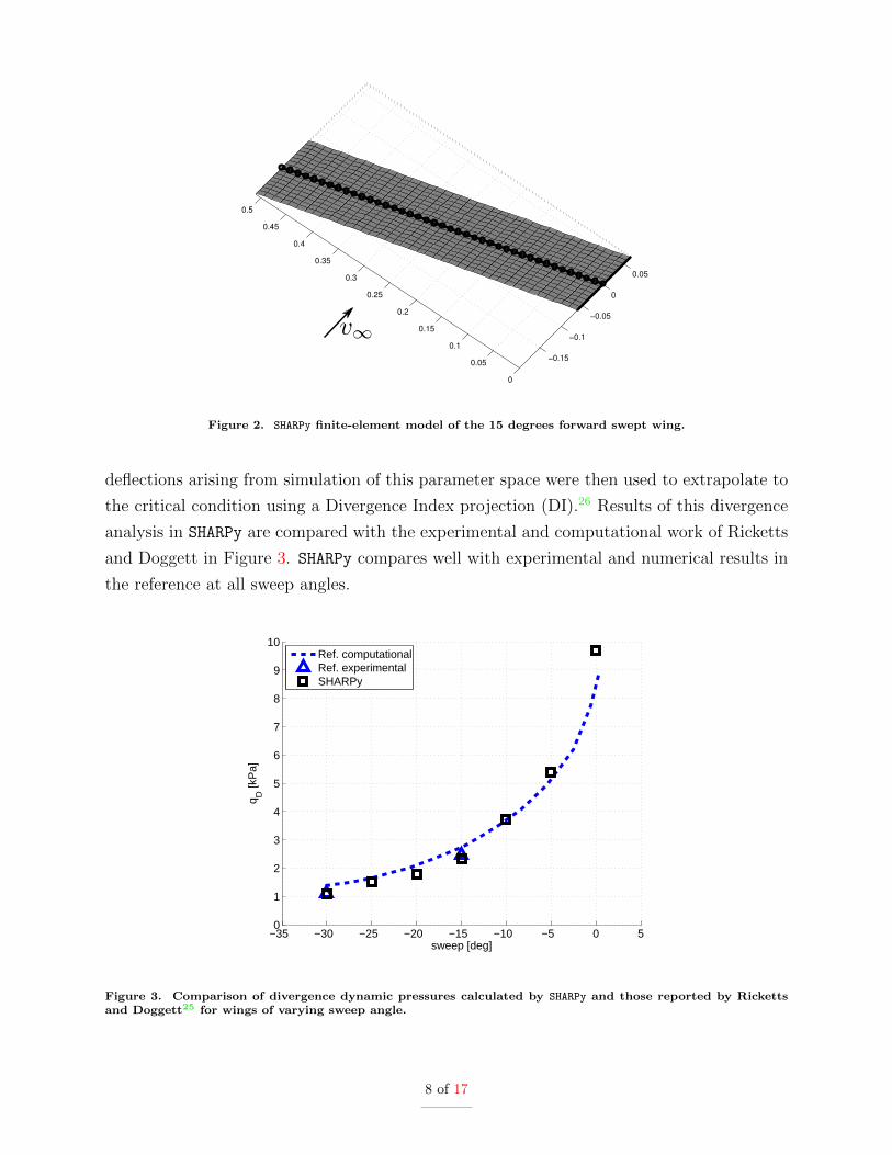
Figure 2. SHARPy finite-element model of the 15 degrees forward swept wing.

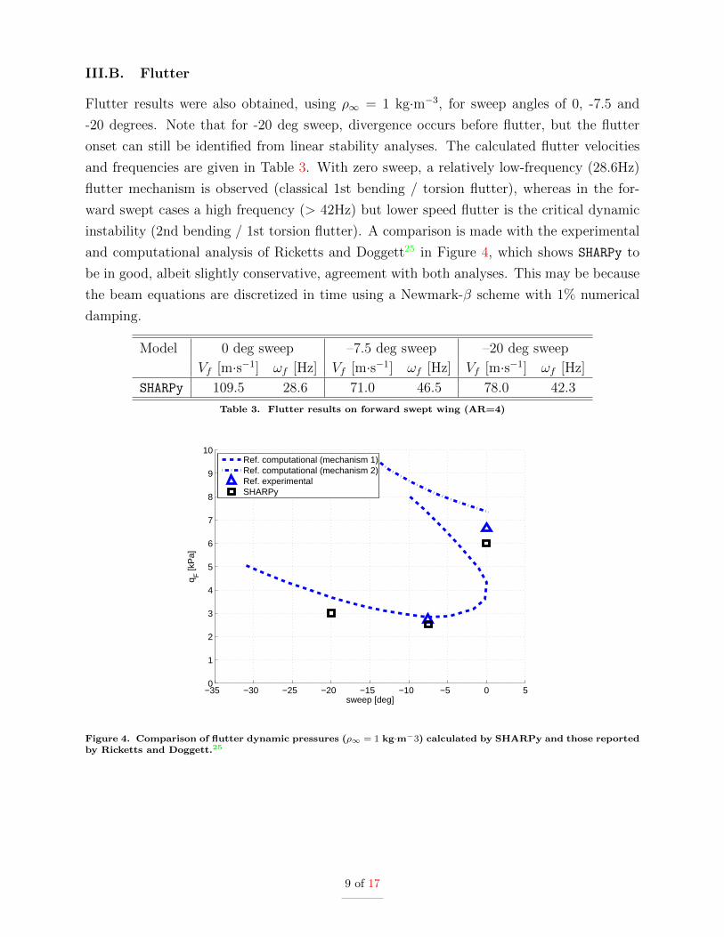
deflections arising from simulation of this parameter space were then used to extrapolate to

the critical condition using a Divergence Index projection (DI).26 Results of this divergence

analysis in SHARPy are compared with the experimental and computational work of Ricketts

and Doggett in Figure 3. SHARPy compares well with experimental and numerical results in

the reference at all sweep angles.

−35 −30 −25 −20 −15 −10 −5 0 50

1

2

3

4

5

6

7

8

9

10

sweep [deg]

q D [k

Pa]

Ref. computationalRef. experimentalSHARPy

Figure 3. Comparison of divergence dynamic pressures calculated by SHARPy and those reported by Rickettsand Doggett25 for wings of varying sweep angle.

8 of 17

III.B. Flutter

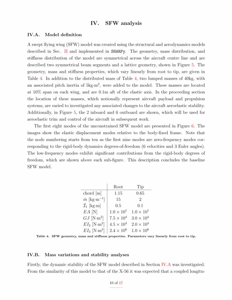
Flutter results were also obtained, using ρ∞ = 1 kg·m−3, for sweep angles of 0, -7.5 and

-20 degrees. Note that for -20 deg sweep, divergence occurs before flutter, but the flutter

onset can still be identified from linear stability analyses. The calculated flutter velocities

and frequencies are given in Table 3. With zero sweep, a relatively low-frequency (28.6Hz)

flutter mechanism is observed (classical 1st bending / torsion flutter), whereas in the for-

ward swept cases a high frequency (> 42Hz) but lower speed flutter is the critical dynamic

instability (2nd bending / 1st torsion flutter). A comparison is made with the experimental

and computational analysis of Ricketts and Doggett25 in Figure 4, which shows SHARPy to

be in good, albeit slightly conservative, agreement with both analyses. This may be because

the beam equations are discretized in time using a Newmark-β scheme with 1% numerical

damping.

Model 0 deg sweep –7.5 deg sweep –20 deg sweep

Vf [m·s−1] ωf [Hz] Vf [m·s−1] ωf [Hz] Vf [m·s−1] ωf [Hz]

SHARPy 109.5 28.6 71.0 46.5 78.0 42.3

Table 3. Flutter results on forward swept wing (AR=4)

−35 −30 −25 −20 −15 −10 −5 0 50

1

2

3

4

5

6

7

8

9

10

sweep [deg]

q F [k

Pa]

Ref. computational (mechanism 1)Ref. computational (mechanism 2)Ref. experimentalSHARPy

Figure 4. Comparison of flutter dynamic pressures (ρ∞ = 1 kg·m−3) calculated by SHARPy and those reportedby Ricketts and Doggett.25

9 of 17

IV. SFW analysis

IV.A. Model definition

A swept flying wing (SFW) model was created using the structural and aerodynamics models

described in Sec. II and implemented in SHARPy. The geometry, mass distribution, and

stiffness distribution of the model are symmetrical across the aircraft centre line and are

described two symmetrical beam segments and a lattice geometry, shown in Figure 5. The

geometry, mass and stiffness properties, which vary linearly from root to tip, are given in

Table 4. In addition to the distributed mass of Table 4, two lumped masses of 40kg, with

an associated pitch inertia of 5kg·m2, were added to the model. These masses are located

at 10% span on each wing, and are 0.1m aft of the elastic axis. In the proceeding section

the location of these masses, which notionally represent aircraft payload and propulsion

systems, are varied to investigated any associated changes to the aircraft aeroelastic stability.

Additionally, in Figure 5, the 2 inboard and 6 outboard are shown, which will be used for

aeroelastic trim and control of the aircraft in subsequent work.

The first eight modes of the unconstrained SFW model are presented in Figure 6. The

images show the elastic displacement modes relative to the body-fixed frame. Note that

the node numbering starts from ten as the first nine modes are zero-frequency modes cor-

responding to the rigid-body dynamics degrees-of-freedom (6 velocities and 3 Euler angles).

The low-frequency modes exhibit significant contributions from the rigid-body degrees of

freedom, which are shown above each sub-figure. This description concludes the baseline

SFW model.

Root Tip

chord [m] 1.15 0.65

m [kg·m−1] 15 2

I1 [kg·m] 0.5 0.1

EA [N] 1.0× 107 1.0× 107

GJ [N·m2] 7.5× 104 3.0× 104

EI2 [N·m2] 4.5× 104 2.0× 104

EI3 [N·m2] 2.4× 106 1.0× 106

Table 4. SFW geometry, mass and stiffness properties. Parameters vary linearly from root to tip.

IV.B. Mass variations and stability analyses

Firstly, the dynamic stability of the SFW model described in Section IV.A was investigated.

From the similarity of this model to that of the X-56 it was expected that a coupled longitu-

10 of 17

dinal rigid-body / 1st symmetric bending mode, i.e. body-freedom flutter (BFF), would be

the critical flutter mode.9 This behaviour is consistent with other recent work on the X-568

and other swept flying-wing configurations.27

To visualize the stability of the aircraft model throughout the flight envelope, linearized

models were constructed for a range of velocities at sea-level air density (ρ∞ = 1.225 kg·m−3).

Eigenvalues of the resulting state transfer matrices (A in Eq. (9)) were then used to construct

root loci illustrating the evolution of the system dynamics with velocity. Figure 7 illustrates

the dynamics of the baseline aircraft, described in Section IV.A, in this way. The short-

period mode rises steadily in frequency and damping from close to the origin far into the

left-hand plane. This is accompanied by the first bending mode (which starts at around 5 Hz)

dropping in frequency and showing a region of decreasing damping (becoming less stable)

after 30 m·s−1. This root migrates into the right-hand plane at around 40 m·s−1, indicating

BFF instability. The coalescence of modal frequencies and divergence of damping – one

mode becoming unstable while the other, in this case the aircraft short period mode, rapidly

becomes very highly damped – is analogous to the classical bend-twist flutter of unswept

cantilever wings. The higher frequency modes of the aircraft remain in the left-hand plane,

and are therefore stable, up to a velocity of 150 m·s−1.

To investigate the effect of mass distribution on the aircraft dynamic stability two modi-

fied SFW models were constructed. This was done by moving the lumped masses from 10%

span (baseline case) to 20% span and 30% span. The chordwise offset of the masses are

updated to maintain a distance of 0.1m from the beam axis. The unconstrained natural

mode frequencies and rigid-body mass properties of all three SFWs are compared in Table

5. Moving the concentrated masses outboard increases the rolling and yawing inertia, and

reduces the pitch inertia.

Figure 8 shows the aeroelastic stability of the baseline model (black), 20% span model

(red) and 30% span model (green). In general the BFF mode velocity is increased as the

lumped masses are moved outboard: 40 m·s−1 for the baseline case, 41 m·s−1 for the 20%

span case, and 52 m·s−1 for the 30% span case. This has the side-effect of introducing a

second, high frequency, instability in the 2nd antisymmetric bending / torsion mode, which

occurs at 150 m·s−1 and 14.3 Hz in the 20% span case. This effect is more pronounced for

the 30% span model where the same mode becomes unstable, but at 120 m·s−1 and 12.45

Hz.

V. Conclusion

A relatively simple swept-flying-wing (SFW) configuration, designed to replicate the sta-

bility problems typical of such aircraft, namely body-freedom-flutter (BFF) and higher fre-

11 of 17

Baseline mode Baseline 20% span 30% span

1sfb 5.15 5.00 5.02

1asfb 8.31 7.05 6.77

2sfb 15.8 16.8 13.9

2asfb/1asT 20.3 17.3 16.9

1sllb 22.2 21.7 23.4

3asfb/2asT 23.7 22.9 24.9

1sT 34.2 35.7 30.3

3asT/3asfb 35.4 37.7 41.1

mtotal [kg] 153.1 153.1 153.1

CoG [% chord] 71.90 79.02 86.17

Iroll [kg·m2] 255.4 293.8 357.8

Ipitch [kg·m2] 28.18 24.35 22.42

Iyaw [kg·m2] 271.0 305.6 367.6

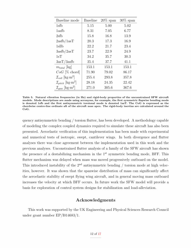
Table 5. Natural vibration frequencies (in Hz) and rigid-body properties of the unconstrained SFW aircraftmodels. Mode descriptions are made using acronyms, for example, the first symmetric flapwise bending modeis denoted 1sfb and the first antisymmetric torsional mode is denoted 1asT. The CoG is expressed as thechordwise centre-line ordinate aft of the aircraft nose apex. The rigid-body inertias are calculated around theCoG.

quency antisymmetric bending / torsion flutter, has been developed. A methodology capable

of modeling the complex coupled dynamics required to simulate these aircraft has also been

presented. Aeroelastic verification of this implementation has been made with experimental

and numerical tests of isotropic, swept, cantilever wings. In both divergence and flutter

analyses there was close agreement between the implementation used in this work and the

previous analyses. Unconstrained flutter analysis of a family of the SFW aircraft has shown

the presence of a destabilizing mechanism in the 1st symmetric bending mode, BFF. This

flutter mechanism was delayed when mass was moved progressively outboard on the model.

This introduced instability of the 2nd antisymmetric bending / torsion mode at high veloc-

ities, however. It was shown that the spanwise distribution of mass can significantly affect

the aeroelastic stability of swept flying wing aircraft, and in general moving mass outboard

increases the velocity at which BFF occurs. In future work the SFW model will provide a

basis for exploration of control system designs for stabilization and load-alleviation.

Acknowledgments

This work was supported by the UK Engineering and Physical Sciences Research Council

under grant number EP/I014683/1.

12 of 17

References

1van Schoor, M. C. and von Flotow, A. H., “Aeroelastic Characteristics of a Highly Flexible Aircraft,”

Journal of Aircraft , Vol. 27, No. 10, 1990, pp. 901 – 908.2Shearer, C. M. and Cesnik, C. E., “Nonlinear flight dynamics of very flexible aircraft,” Journal of

Aircraft , Vol. 44, No. 5, 2007, pp. 1528 – 1545.3Jian, Z. and Jinwu, X., “Nonlinear Aeroelastic Response of High-aspect-ratio Flexible Wings,” Chinese

Journal of Aeronautics, Vol. 22, No. 4, Aug. 2009, pp. 355 – 363.4Wang, Z., Chen, P. C., Liu, D. D., and Mook, D. T., “Nonlinear-Aerodynamics/Nonlinear-Structure

Interaction Methodology for a High-Altitude Long-Endurance Wing,” Journal of aircraft , Vol. 47, No. 2,

2010, pp. 556 – 566.5Su, W. and Cesnik, C. E. S., “Dynamic Response of Highly Flexible Flying Wings,” AIAA Journal ,

Vol. 49, No. 2, 2011, pp. 324 – 339.6Dillsaver, M. J., Cesnik, C. E. S., and Kolmanovsky, I. V., “Gust Response Sensitivity Characteristics

of Very Flexible Aircraft,” AIAA Atmospheric Flight Mechanics Conference, AIAA, Minneapolis, Minnesota,

Aug. 2012.7Cesnik, C. E., Senatore, P. J., Weihua, S., Atkins, E. M., and Shearer, C. M., “X-HALE: A Very

Flexible Unmanned Aerial Vehicle for Nonlinear Aeroelastic Tests,” AIAA journal , Vol. 50, No. 12, 2012,

pp. 2820 – 2833.8Ryan, J. J., Bosworth, J. T., Burken, J. J., and Suh, P. M., “Current and Future Research in Active

Control of Lightweight, Flexible Structures Using the X-56 Aircraft,” 52nd Aerospace Sciences Meeting at

SciTech, AIAA, National Harbour, MD, Jan. 2014.9Bryson, D. E. and Alyanak, E. J., “Aeroelastic Modeling of the X-56A Using a Rapid Model Generator

for Conceptual Design,” 52nd Aerospace Sciences Meeting at SciTech, AIAA, National Harbour, MD, Jan.

2014.10Hjartarson, A., Seiler, P. J., and Balas, G. J., “LPV aeroservoelastic control using the lpvtools toolbox,”

AIAA Atmospheric Flight Mechanics Conference, AIAA, Boston, MA, Aug. 2013.11Hodges, D. H., “A mixed variational formulation based on exact intrinsic equations for dynamics of

moving beams,” International Journal of Solids and Structures, Vol. 26, No. 11, 1990, pp. 1253 – 1273.12Geradin, M. and Cardona, A., Flexible Multibody Dynamics: A Finite Element Approach, John Wiley

& Sons Ltd, Chichester, UK, 2001.13Hesse, H. and Palacios, R., “Consistent structural linearisation in flexible-body dynamics with large

rigid-body motion,” Computers & Structures, Vol. 110 - 111, 2012, pp. 1 – 14.14Stevens, B. L. and Lewis, F. L., Aircraft Control and Simulation, John Wiley & Sons, Inc., New York,

NY, USA, 1992.15Murua, J., Hesse, H., Palacios, R., and Graham, J. M. R., “Stability and Open-Loop Dynamics of Very

Flexible Aircraft Including Free-Wake Effects,” 52nd AIAA/ASME/ASCE/AHS/ASC Structures, Structural

Dynamics and Materials Conference, Denver, Colorado, April 2011.16Morino, L. and Bernardini, G., “Singularities in BIEs for the Laplace equation; Joukowski trailing-edge

conjecture revisited,” Engineering Analysis with Boundary Elements, Vol. 25, No. 9, Oct. 2001, pp. 805 –

818.17Katz, J. and Plotkin, A., Low-Speed Aerodynamics, Cambridge University Press, 2001.18Murua, J., Flexible Aircraft Dynamics with a Geometrically-Nonlinear Description of the Unsteady

Aerodynamics, Ph.D. thesis, Imperial College London, Department of Aeronautics, May 2012.19Simpson, R. J. S., Palacios, R., Hesse, H., and Goulart, P. J., “Predictive Control for Alleviation of Gust

13 of 17

Loads on Very Flexible Aircraft,” 55th AIAA/ASME/ASCE/AHS/ASC Structures, Structural Dynamics,

and Materials Conference at SciTech, AIAA, National Harbour, MA, Jan. 2014.20Simpson, R. J. S., Palacios, R., and Murua, J., “Induced Drag Calculations in the Unsteady Vortex

Lattice Method,” AIAA Journal , Vol. 51, No. 7, 2013, pp. 1775 – 1779.21Simpson, R. J. S. and Palacios, R., “Numerical aspects of nonlinear flexible aircraft flight dynamics

modeling,” 54th AIAA/ASME/ASCE/AHS/ASC Structures, Structural Dynamics, and Materials Confer-

ence, AIAA, Boston, MA, April 2013.22Cook, R., Palacios, R., and Goulart, P., “Robust Gust Alleviation and Stabilization of Very Flexible

Aircraft,” AIAA Journal , Vol. 51, No. 2, February 2013, pp. 330 – 340.23Murua, J., Palacios, R., and Graham, J. M. R., “Applications of the unsteady vortex-lattice method

in aircraft aeroelasticity and flight dynamics,” Progress in Aerospace Sciences, Vol. 55, Nov. 2012, pp. 46 –

72.24Hall, K. C., “Eigenanalysis of unsteady flows about airfoils, cascades, and wings,” AIAA journal ,

Vol. 32, 1994, pp. 2426 – 2432.25Ricketts, R. H. and Doggett, R. V., “Wind-tunnel experiments on divergence of forward-swept wings,”

Technical Paper TP 1685, NASA, Langley Research Center, Hampton, VA, 1980.26Hertz, T. J., Shirk, M. H., Ricketts, R. H., and Weisshaar, T. A., “Aeroelastic tailoring with composites

applied to forward swept wings,” Tech. Rep. AFWAL-TR-81-3043, DTIC Document, 1981.27Love, M. H., Zink, P. S., Wieselmann, P. A., and Youngren, H., “Body freedom flutter of high as-

pect ratio flying wings,” The 46th AIAA/ASME/ASCE/AHS/ASC Structures, Structural Dynamics and

Materials Conference, AIAA, Austin, Texas, April 2005.

14 of 17

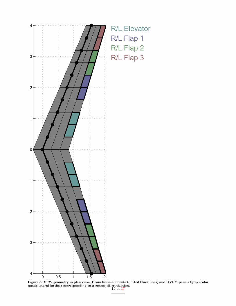
Figure 5. SFW geometry in plan view. Beam finite-elements (dotted black lines) and UVLM panels (gray/colorquadrilateral lattice) corresponding to a coarse discretization.

15 of 17

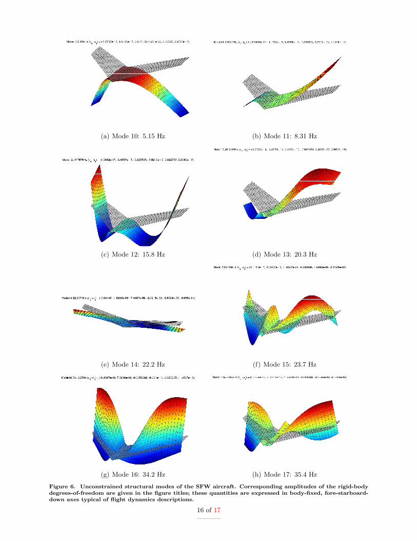
(a) Mode 10: 5.15 Hz (b) Mode 11: 8.31 Hz

(c) Mode 12: 15.8 Hz (d) Mode 13: 20.3 Hz

(e) Mode 14: 22.2 Hz (f) Mode 15: 23.7 Hz

(g) Mode 16: 34.2 Hz (h) Mode 17: 35.4 Hz

Figure 6. Unconstrained structural modes of the SFW aircraft. Corresponding amplitudes of the rigid-bodydegrees-of-freedom are given in the figure titles; these quantities are expressed in body-fixed, fore-starboard-down axes typical of flight dynamics descriptions.

16 of 17

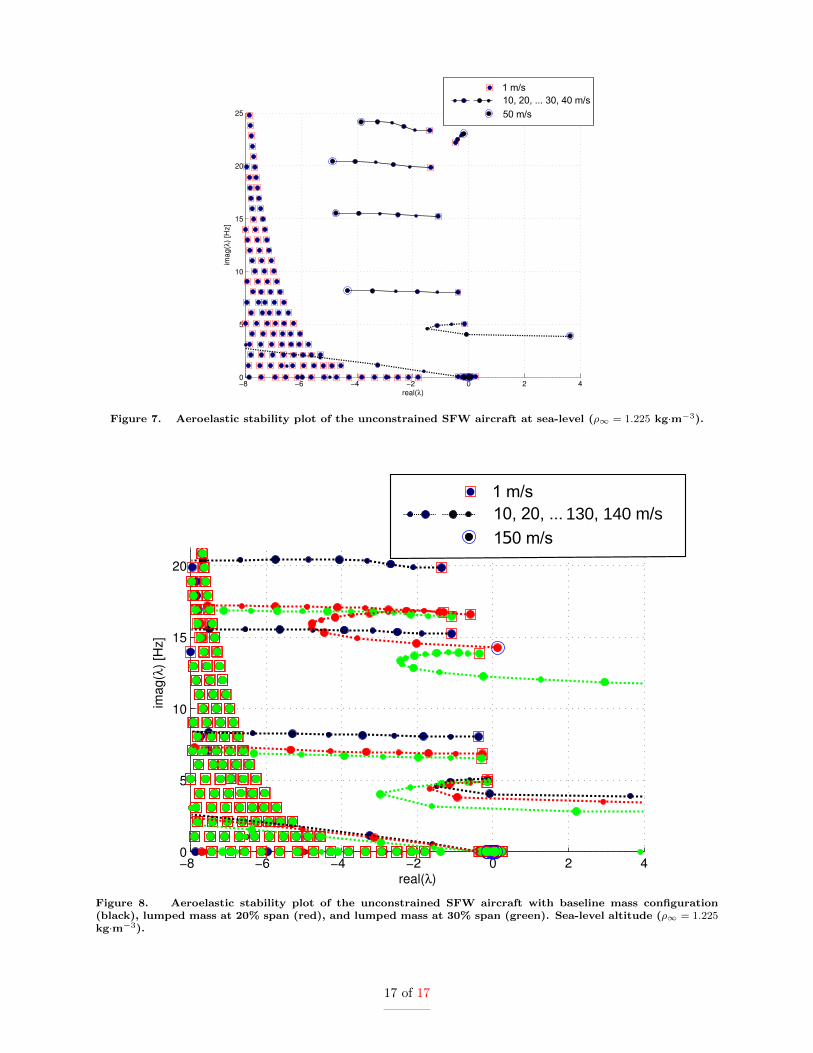
Figure 7. Aeroelastic stability plot of the unconstrained SFW aircraft at sea-level (ρ∞ = 1.225 kg·m−3).

Figure 8. Aeroelastic stability plot of the unconstrained SFW aircraft with baseline mass configuration(black), lumped mass at 20% span (red), and lumped mass at 30% span (green). Sea-level altitude (ρ∞ = 1.225kg·m−3).

17 of 17