Integrated energy and battery life management for … · Integrated energy and battery life...
139
Integrated energy and battery life management for hybrid vehicles Pham, H.T. Published: 28/04/2015 Document Version Publisher’s PDF, also known as Version of Record (includes final page, issue and volume numbers) Please check the document version of this publication: • A submitted manuscript is the author's version of the article upon submission and before peer-review. There can be important differences between the submitted version and the official published version of record. People interested in the research are advised to contact the author for the final version of the publication, or visit the DOI to the publisher's website. • The final author version and the galley proof are versions of the publication after peer review. • The final published version features the final layout of the paper including the volume, issue and page numbers. Link to publication Citation for published version (APA): Pham, H. T. (2015). Integrated energy and battery life management for hybrid vehicles Eindhoven: Technische Universiteit Eindhoven General rights Copyright and moral rights for the publications made accessible in the public portal are retained by the authors and/or other copyright owners and it is a condition of accessing publications that users recognise and abide by the legal requirements associated with these rights. • Users may download and print one copy of any publication from the public portal for the purpose of private study or research. • You may not further distribute the material or use it for any profit-making activity or commercial gain • You may freely distribute the URL identifying the publication in the public portal ? Take down policy If you believe that this document breaches copyright please contact us providing details, and we will remove access to the work immediately and investigate your claim. Download date: 08. Sep. 2018
Transcript of Integrated energy and battery life management for … · Integrated energy and battery life...
Integrated energy and battery life management for hybridvehiclesPham, H.T.
Published: 28/04/2015
Document VersionPublisher’s PDF, also known as Version of Record (includes final page, issue and volume numbers)
Please check the document version of this publication:
• A submitted manuscript is the author's version of the article upon submission and before peer-review. There can be important differencesbetween the submitted version and the official published version of record. People interested in the research are advised to contact theauthor for the final version of the publication, or visit the DOI to the publisher's website.• The final author version and the galley proof are versions of the publication after peer review.• The final published version features the final layout of the paper including the volume, issue and page numbers.
Link to publication
Citation for published version (APA):Pham, H. T. (2015). Integrated energy and battery life management for hybrid vehicles Eindhoven: TechnischeUniversiteit Eindhoven
General rightsCopyright and moral rights for the publications made accessible in the public portal are retained by the authors and/or other copyright ownersand it is a condition of accessing publications that users recognise and abide by the legal requirements associated with these rights.
• Users may download and print one copy of any publication from the public portal for the purpose of private study or research. • You may not further distribute the material or use it for any profit-making activity or commercial gain • You may freely distribute the URL identifying the publication in the public portal ?
Take down policyIf you believe that this document breaches copyright please contact us providing details, and we will remove access to the work immediatelyand investigate your claim.
Download date: 08. Sep. 2018

It is my pleasure to invite you to the defense of my
PhD dissertation
Integrated energy and battery life
management for hybrid vehicles
In room 4 of the Auditorium of Eindhoven University
of Technology
on Tuesday28 April 2015
at 16:00.
You are also cordially invited to the reception that will
follow at Senaatzaal of the Auditorium.
Pham Hong [email protected]
± 130 pag.= 8,3mm rug90 grs. BiotopGlanslaminaat
Integrated Energy and Battery Life
Management for Hybrid Vehicles
PROEFSCHRIFT
ter verkrijging van de graad van doctor aan de Technische Universiteit
Eindhoven, op gezag van de rector magnificus, prof.dr.ir. C.J. van Duijn,
voor een commissie aangewezen door het College voor Promoties, in het
openbaar te verdedigen op dinsdag 28 april 2015 om 16:00 uur
door
Pham Hong Thinh
geboren te Bac Ninh, Vietnam

Dit proefschrift is goedgekeurd door de promotoren en de samenstelling van de pro-
motiecommissie is als volgt:
voorzitter: prof.dr.ir. A.C.P.M. Backx
1e promotor: prof.dr.ir. P.P.J. van den Bosch
co-promotor(en): dr.ir. J.T.B.A. Kessels
leden: prof.dr.ir. E.G.M. Holweg (TUD)
prof.dr. A. Bouscayrol (Universite Lille 1)
prof.dr.ir. M. Steinbuch
dr.ir. A.G. de Jager
adviseur(s): dr.ir. R.G.M. Huisman (DAF Trucks N.V.)

Integrated Energy and Battery Life
Management for Hybrid Vehicles
This work has been carried out as part of the Hybrid
Innovations for Trucks (HIT) project, which is funded by HTAS.
This dissertation has been completed in fulfillment of the
requirements of the Dutch Institute of Systems and Control DISC.
This thesis was prepared using the LATEX typesetting system.
Printed by: Printservice, Eindhoven University of Technology.
Cover design: Paul Verspaget, Nuenen, The Netherlands.
A catalogue record is available from the Eindhoven University of Technology Library.
Integrated energy and battery life management for hybrid vehicles
by Pham Hong Thinh. - Eindhoven: Technische Universiteit Eindhoven, 2015.
Proefschrift.
ISBN: 978-90-386-3822-5
NUR: 951
Copyright c©2015 by Pham Hong Thinh

This thesis is dedicated to my beloved family
iii

Summary
Integrated Energy and Battery Life Management for Hybrid Vehicles
Over the years, Hybrid Electric Vehicles (HEVs) have emerged as a leading technol-
ogy to satisfy the future market’s fuel consumption and emission demands. In HEVs,
an Internal Combustion Engine (ICE) cooperates with a high-voltage battery to bring
opportunities in reducing its fuel consumption and the associated CO2 emission. The
cooperative operation of the ICE and the battery is handled by a sophisticated Energy
Management Strategy (EMS) to minimize the HEVs’ fuel consumption.
This thesis presents a Hybrid Electric Truck with a clutch system consisting of an ICE
clutch and a Motor Generator (MG) clutch. The clutch system enables the capability
for decoupling the ICE and MG from the Drivetrain. As a result, it offers opportunities
for improving the fuel reduction by eliminating the parasitic drag losses in the ICE and
MG.
The objective of the EMS is to determine the power/torque split between the ICE and
the MG by influencing the battery charge/discharge power and clutches selection. How-
ever, battery usage shortens battery life and incurs extra costs for battery replacement.
By restricting the usage of the battery, the battery life can be prolonged with a penalty
on the total fuel consumption of the hybrid truck. Henceforth, operation of the EMS
and the battery life management are not separated.
This thesis has developed an Integrated Energy Management (IEM) strategy to guaran-
tee the requested battery life and to minimize the vehicle fuel consumption by optimizing
the battery charge/discharge power and the operation of the clutch system. The solu-
tion of the IEM strategy is analytical and yields both mathematical and physical insight
regarding the balance between fuel reduction and battery life preservation. The derived
solution of the IEM is computational very efficient.
The analytical solution of this IEM strategy requires prior knowledge, especially the
driving cycle, to find their optimal control variables. As a result, they are non-causal
strategies. This thesis has developed a real-time implementable IEM strategy satisfy-
ing the battery life requirement while minimizing the fuel consumption. The control
v
variables of the real-time implementable IEM strategy are estimated online using a
combination of feedforward and feedback control. The feedforward controller utilizes
Driving Pattern Recognition (DPR) techniques to provide the current driving pattern.
The optimal control variables are found off-line using the analytical solutions of the IEM
strategy for predefined standard driving cycles, being stored in look-up tables. Due to
the inaccuracy of the DPR, and the differences between the models and the actual pro-
cess, feedback loops from system states are constructed to keep the system states around
their predefined reference trajectories.
In summary, the main contributions of this thesis are:
• An analytical solution for integrated energy management of a hybrid truck with
the option of an additional clutch to decouple and turn off the MG from the
drivetrain when it is not used. The optimal battery charge/discharge power and
the operation of the clutch system are found to minimize the fuel consumption
whilst satisfying the battery life requirement with the assumption that the exact
information of the future driving cycle is known.
• A real-time implementable solution of the integrated energy management for a
hybrid truck to guarantee the battery life requirement while minimizing the vehi-
cle fuel consumption. The real-time implementable solution optimizes the battery
charge/discharge power and the clutches’ operation without requiring exact infor-
mation of the future driving cycle.
Contents
Summary v
Contents vii
Abbreviations xi
1 Introduction 1
1.1 Research motivation . . . . . . . . . . . . . . . . . . . . . . . . . . . . . . 1
1.1.1 Advances in hybrid trucks . . . . . . . . . . . . . . . . . . . . . . . 1
1.1.2 Motivation for integrated energy and battery wear management . . 3
1.2 Powertrain configuration of hybrid electric truck . . . . . . . . . . . . . . 4
1.3 Research objectives . . . . . . . . . . . . . . . . . . . . . . . . . . . . . . . 7
1.4 Problem definition . . . . . . . . . . . . . . . . . . . . . . . . . . . . . . . 7
1.5 Literature survey . . . . . . . . . . . . . . . . . . . . . . . . . . . . . . . . 11
1.5.1 Energy management in hybrid electric vehicles . . . . . . . . . . . 11
1.5.2 Integrated Energy Management in hybrid electric vehicles . . . . . 13
1.6 Thesis outline . . . . . . . . . . . . . . . . . . . . . . . . . . . . . . . . . . 15
2 System modeling 17
2.1 Vehicle model . . . . . . . . . . . . . . . . . . . . . . . . . . . . . . . . . . 17
2.2 Internal combustion engine model . . . . . . . . . . . . . . . . . . . . . . . 19
2.3 Motor generator model . . . . . . . . . . . . . . . . . . . . . . . . . . . . . 21
2.4 Battery model . . . . . . . . . . . . . . . . . . . . . . . . . . . . . . . . . 23
2.4.1 Battery efficiency model . . . . . . . . . . . . . . . . . . . . . . . . 23
2.4.2 Quasi-static battery cycle-life model . . . . . . . . . . . . . . . . . 26
2.5 Conclusions . . . . . . . . . . . . . . . . . . . . . . . . . . . . . . . . . . . 30
3 Analytical solutions for energy management 31
3.1 Analytical solution for energy management without battery life requirement 32
3.1.1 Explicit solution for energy management during driving periods . . 33
3.1.2 Optimal battery power during braking periods . . . . . . . . . . . 38
3.2 Solution for energy management with battery energy state constraint andwithout battery life requirement . . . . . . . . . . . . . . . . . . . . . . . 39
3.3 Analytical solution for integrated energy management . . . . . . . . . . . 40
3.3.1 Convexification of battery cycle-life model . . . . . . . . . . . . . . 40
3.3.2 Extended equivalent fuel consumption management strategy ap-proach . . . . . . . . . . . . . . . . . . . . . . . . . . . . . . . . . . 42
vii
Contents viii
3.3.3 Explicit solution for integrated energy management during drivingperiods . . . . . . . . . . . . . . . . . . . . . . . . . . . . . . . . . 44
3.3.4 Optimal battery power during braking periods . . . . . . . . . . . 47
3.3.5 Effect of integrated energy management strategy on preservingbattery life . . . . . . . . . . . . . . . . . . . . . . . . . . . . . . . 47
3.3.5.1 Influence of IEM1 strategy on battery usage in MA, Cand R mode . . . . . . . . . . . . . . . . . . . . . . . . . 48
3.3.5.2 Influence of IEM1 strategy on battery usage in MO mode 48
3.3.5.3 Influence of IEM1 strategy on battery usage in PSM andICE Only mode . . . . . . . . . . . . . . . . . . . . . . . 49
3.4 Solution for integrated energy management with battery energy state con-straint . . . . . . . . . . . . . . . . . . . . . . . . . . . . . . . . . . . . . . 53
3.5 Integrated energy and thermal management including battery wear . . . . 53
3.6 Conclusions . . . . . . . . . . . . . . . . . . . . . . . . . . . . . . . . . . . 56
4 Real-time implementation of adaptive integrated energy management 59
4.1 Motivation for adaptive integrated energy management . . . . . . . . . . . 59
4.2 Real-time implementation concept . . . . . . . . . . . . . . . . . . . . . . 61
4.3 Driving pattern recognition . . . . . . . . . . . . . . . . . . . . . . . . . . 63
4.3.1 Principal component analysis . . . . . . . . . . . . . . . . . . . . . 63
4.3.2 Verification of driving pattern recognition algorithm . . . . . . . . 66
4.4 Feedback control concept for adaptive energy management . . . . . . . . . 68
4.4.1 Bandwidth of energy management strategy . . . . . . . . . . . . . 68
4.4.2 Adaptive tuning scheme for PI controller . . . . . . . . . . . . . . 71
4.5 Computation of cost-effective battery power range . . . . . . . . . . . . . 73
4.6 Conclusions . . . . . . . . . . . . . . . . . . . . . . . . . . . . . . . . . . . 75
5 Simulation results 77
5.1 Fuel reduction improvement from Motor Generator clutch . . . . . . . . . 78
5.2 Integrated energy management strategy performance . . . . . . . . . . . . 80
5.3 Energy management strategy performance for keeping battery energy inpredefined window . . . . . . . . . . . . . . . . . . . . . . . . . . . . . . . 85
5.4 Performance of the adaptive integrated energy management strategy . . . 85
5.4.1 Constraint handling . . . . . . . . . . . . . . . . . . . . . . . . . . 87
5.4.2 Influence of battery capacity loss reference trajectory . . . . . . . . 89
5.5 Conclusions . . . . . . . . . . . . . . . . . . . . . . . . . . . . . . . . . . . 91
6 Conclusions and recommendations 93
6.1 Conclusions . . . . . . . . . . . . . . . . . . . . . . . . . . . . . . . . . . . 93
6.2 Recommendations . . . . . . . . . . . . . . . . . . . . . . . . . . . . . . . 95
A Mathematical derivation of energy management without battery lifepreservation 97
A.1 Optimal battery power in MA and C mode for CEM1 . . . . . . . . . . . 97
A.2 Hamiltonian function minimization for CEM1 . . . . . . . . . . . . . . . . 98
A.3 Influence of battery power loss coefficient on CEM1 . . . . . . . . . . . . . 99
Contents ix
B Mathematical derivation of integrated energy management with bat-tery life preservation 103
B.1 Optimal battery power in MA and C mode for IEM1 . . . . . . . . . . . . 103
B.2 Hamiltonian function minimization for IEM1 . . . . . . . . . . . . . . . . 104
B.3 Influence of FF and FB control on A-IEM strategy performance . . . . . . 106
B.4 Benefit and cost for battery usage in MA, MO and R mode . . . . . . . . 110
B.5 Computation of battery capacity loss upper bound . . . . . . . . . . . . . 112
Bibliography 113
Acknowledgments 121
Curriculum Vitae 123

Abbreviations
A-IEM Adaptive Integrated Energy Management
BTMS Battery Thermal Management System
BTS Battery Thermal System
DOC Diesel Oxidation Catalyst
DPR Driving Pattern Recognition
ECMS Equivalent fuel Consumption Management Strategy
EMS Energy Management Strategy
GHG Green House Gases
GPS Global Positioning System
HEV Hybrid Electric Vehicle
ICE Internal Combustion Engine
IEM Integrated Energy Management
IETM Integrated Energy and battery Thermal Management
IPC Integrated Powertrain Control
ITS Intelligent Transportation System
PC Principle Component
PCA Principal Component Analysis
SCR Selective Catalytic Reduction
xi

Chapter 1
Introduction
1.1 Research motivation
This section presents the motivation for using hybrid electric powertrain technology in
a heavy-duty truck, and the necessity for integrating battery lifetime management into
the energy management system of a hybrid truck.
1.1.1 Advances in hybrid trucks
Over decades, the global warming and the shortage of fossil fuels have been two of the
critical issues for mankind. As reported by the US Energy Information Administration
(EIA), in 2013, fossil fuels amounted up to 82% percent share of the total primary
energy consumption in the world1. Fossil fuels are typically burned to generate the
energy. This burning process emits Green House Gases (GHG), primarily CO2, which
cannot be absorbed entirely by natural processes. It results in a net-increase of GHG in
the atmosphere. The total CO2 emission in the world is doubled in the period from 1971
to 2010 [1]. It is stated in [2] that this net-increase of GHG in the atmosphere is one of
the main global warming sources. To protect our environment and achieve a sustainable
energy society, it is essential to prevent GHG from emitting to the environment and to
restrict the fossil fuels consumption [2], [3].
According to the International Energy Agency (IEA), transportation is an important
cause of the global CO2 emissions, accounted for 22% of the world CO2 emission in 2010.
Within the transportation itself, long haul applications contribute about 80% of the
total CO2 emissions of commercial vehicles. More generally, in developing commercial
vehicles, one of the most crucial objectives is reducing the vehicle fuel consumption and
1The data is available at the US EIA, www.eia.gov/totalenergy/
1
1.1. Research motivation
so CO2 emission. Fuel consumption is an important variable cost in the transportation
and logistic industry [4]. It is both desired and necessary to reduce the fuel consumption
and the associated CO2 emission of the vehicle in long haul applications.
Approaches, reducing the fuel consumption of long haul vehicles, can be classified into
three main categories (see [5] and the references there in),
• efficiency-improving technologies non-electric on conventional powertrains and ve-
hicles
• substitution of natural gas, electricity or hydrogen for diesel fuel
• hybrid drive technologies
These approaches have their own potential for lowering the fuel consumption and the
associated CO2 emission. This thesis focuses on the third item: hybrid drive technolo-
gies.
Hybrid drive technology is a viable solution to reduce the vehicle fuel consumption and
comply with increasingly stringent emission legislation. In hybrid vehicles, an Internal
Combustion Engine (ICE) cooperates with an additional power source to bring oppor-
tunities in minimizing fuel consumption and associated CO2 emission. Over the last
decade, many Hybrid Electric Vehicles (HEVs) have been produced in series in the
passenger car market (light-duty) [6], e.g., Citroen C3, Honda Civic IMA, Toyota Prius.
In the class of medium-duty trucks and buses, HEVs are also in production for several
years, e.g., DAF LF, Volvo hybrid bus. However, despite its significant fuel consumption
reduction (between 20 and 30% [7]), the production numbers are low due to the high
additional cost of a hybrid system.
Utilization of hybrid drive technology in heavy-duty trucks, on the other hand, is still
in the development stage. Although these vehicles normally drive on the highway with
minimum braking and acceleration events, one of the benefits from hybridization comes
from its huge vehicle’s mass (up to 40 tons). Specifically, when the truck reduces its
speed or goes downhill, there emerges considerable braking energy to be absorbed in
a dedicated battery for later utilization. Besides, the potential for using hybrid drive
technology in long haul trucks comes from its high mileage, e.g., 150, 000 km/year. The
potential fuel benefit depends also on many design aspects of the hybrid power train.
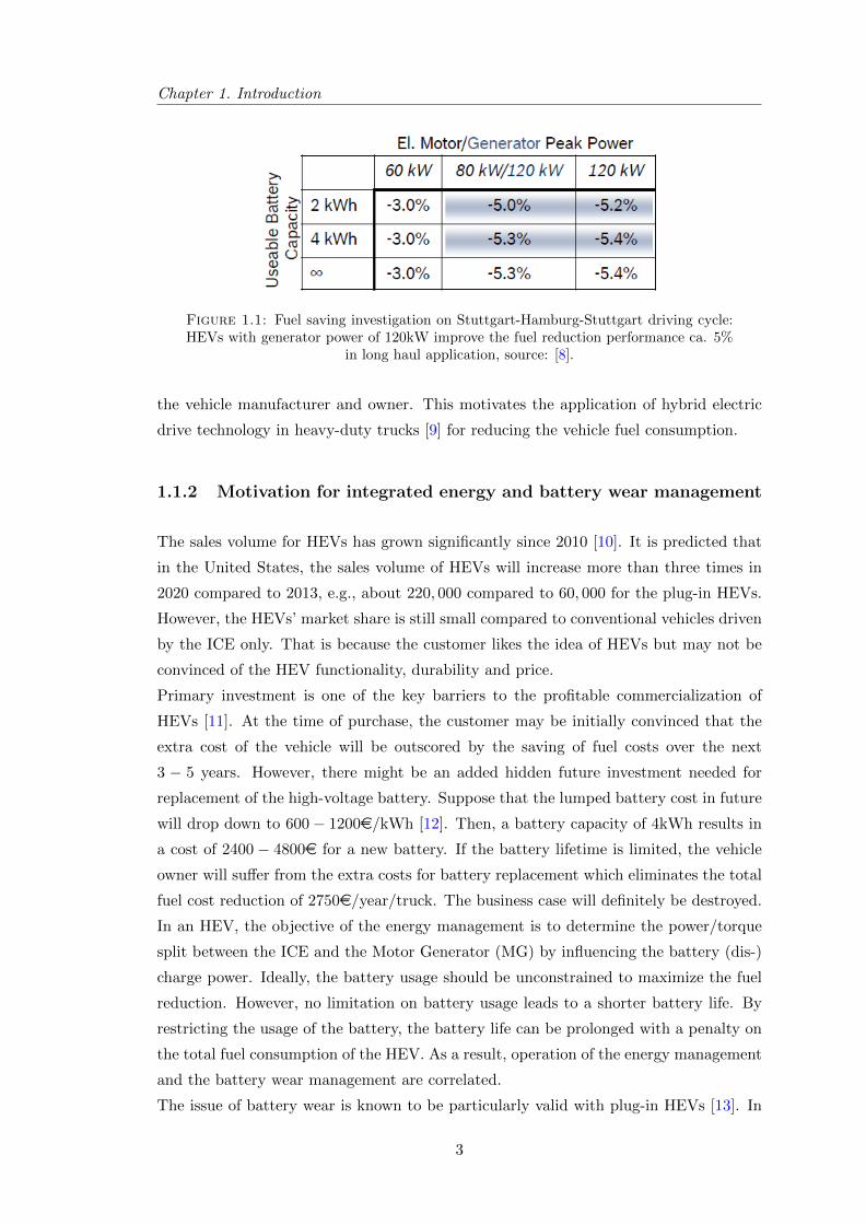
A study from Bosch [8] reveals that battery storage capacity and power ratings of the
electric machine influence on the actual fuel savings, see Fig. 1.1. Suppose a hybrid
truck saves 5% fuel consumption compared to a conventional truck (driven by the ICE
only). A conventional truck consumes on average 33 liters/100km, resulting in about
50, 000 liters of diesel per year [7]. With a diesel price of 1.1[e/liter], the total fuel cost
reduction per year per truck is translated into 2750[e] which is considerable for both
2
Chapter 1. Introduction
Figure 1.1: Fuel saving investigation on Stuttgart-Hamburg-Stuttgart driving cycle:HEVs with generator power of 120kW improve the fuel reduction performance ca. 5%
in long haul application, source: [8].
the vehicle manufacturer and owner. This motivates the application of hybrid electric
drive technology in heavy-duty trucks [9] for reducing the vehicle fuel consumption.
1.1.2 Motivation for integrated energy and battery wear management
The sales volume for HEVs has grown significantly since 2010 [10]. It is predicted that
in the United States, the sales volume of HEVs will increase more than three times in
2020 compared to 2013, e.g., about 220, 000 compared to 60, 000 for the plug-in HEVs.
However, the HEVs’ market share is still small compared to conventional vehicles driven
by the ICE only. That is because the customer likes the idea of HEVs but may not be
convinced of the HEV functionality, durability and price.
Primary investment is one of the key barriers to the profitable commercialization of
HEVs [11]. At the time of purchase, the customer may be initially convinced that the
extra cost of the vehicle will be outscored by the saving of fuel costs over the next
3 − 5 years. However, there might be an added hidden future investment needed for
replacement of the high-voltage battery. Suppose that the lumped battery cost in future
will drop down to 600− 1200e/kWh [12]. Then, a battery capacity of 4kWh results in
a cost of 2400 − 4800e for a new battery. If the battery lifetime is limited, the vehicle
owner will suffer from the extra costs for battery replacement which eliminates the total
fuel cost reduction of 2750e/year/truck. The business case will definitely be destroyed.
In an HEV, the objective of the energy management is to determine the power/torque
split between the ICE and the Motor Generator (MG) by influencing the battery (dis-)
charge power. Ideally, the battery usage should be unconstrained to maximize the fuel
reduction. However, no limitation on battery usage leads to a shorter battery life. By
restricting the usage of the battery, the battery life can be prolonged with a penalty on
the total fuel consumption of the HEV. As a result, operation of the energy management
and the battery wear management are correlated.
The issue of battery wear is known to be particularly valid with plug-in HEVs [13]. In
3
1.2. Powertrain configuration of hybrid electric truck
hybrid electric trucks, to compromise the total operational cost for vehicle owner, the
balance between fuel consumption reduction, battery cost and battery life should be
carefully considered [14]. It is necessary to integrate the battery wear management into
the energy management system of hybrid trucks.
1.2 Powertrain configuration of hybrid electric truck
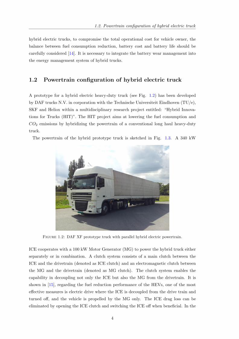
A prototype for a hybrid electric heavy-duty truck (see Fig. 1.2) has been developed
by DAF trucks N.V. in corporation with the Technische Universiteit Eindhoven (TU/e),
SKF and Heliox within a multidisciplinary research project entitled: “Hybrid Innova-
tions for Trucks (HIT)”. The HIT project aims at lowering the fuel consumption and
CO2 emissions by hybridizing the powertrain of a conventional long haul heavy-duty
truck.
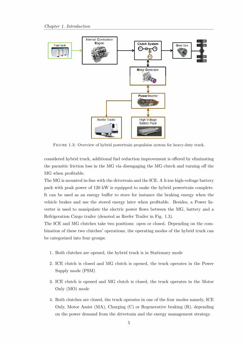
The powertrain of the hybrid prototype truck is sketched in Fig. 1.3. A 340 kW
Figure 1.2: DAF XF prototype truck with parallel hybrid electric powertrain.
ICE cooperates with a 100 kW Motor Generator (MG) to power the hybrid truck either
separately or in combination. A clutch system consists of a main clutch between the
ICE and the drivetrain (denoted as ICE clutch) and an electromagnetic clutch between
the MG and the drivetrain (denoted as MG clutch). The clutch system enables the
capability in decoupling not only the ICE but also the MG from the drivetrain. It is
shown in [15], regarding the fuel reduction performance of the HEVs, one of the most
effective measures is electric drive where the ICE is decoupled from the drive train and
turned off, and the vehicle is propelled by the MG only. The ICE drag loss can be
eliminated by opening the ICE clutch and switching the ICE off when beneficial. In the
4
Chapter 1. Introduction
Figure 1.3: Overview of hybrid powertrain propulsion system for heavy-duty truck.
considered hybrid truck, additional fuel reduction improvement is offered by eliminating
the parasitic friction loss in the MG via disengaging the MG clutch and turning off the
MG when profitable.
The MG is mounted in-line with the drivetrain and the ICE. A li-ion high-voltage battery
pack with peak power of 120 kW is equipped to make the hybrid powertrain complete.
It can be used as an energy buffer to store for instance the braking energy when the
vehicle brakes and use the stored energy later when profitable. Besides, a Power In-
verter is used to manipulate the electric power flows between the MG, battery and a
Refrigeration Cargo trailer (denoted as Reefer Trailer in Fig. 1.3).
The ICE and MG clutches take two positions: open or closed. Depending on the com-
bination of these two clutches’ operations, the operating modes of the hybrid truck can
be categorized into four groups:
1. Both clutches are opened, the hybrid truck is in Stationary mode
2. ICE clutch is closed and MG clutch is opened, the truck operates in the Power
Supply mode (PSM)
3. ICE clutch is opened and MG clutch is closed, the truck operates in the Motor
Only (MO) mode
4. Both clutches are closed, the truck operates in one of the four modes namely, ICE
Only, Motor Assist (MA), Charging (C) or Regenerative braking (R), depending
on the power demand from the drivetrain and the energy management strategy.
5
1.2. Powertrain configuration of hybrid electric truck
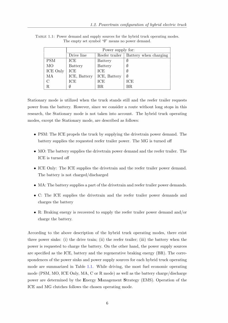
Table 1.1: Power demand and supply sources for the hybrid truck operating modes.The empty set symbol “∅” means no power demand.
Power supply for:
Drive line Reefer trailer Battery when charging
PSM ICE Battery ∅MO Battery Battery ∅ICE Only ICE ICE ∅MA ICE, Battery ICE, Battery ∅C ICE ICE ICER ∅ BR BR
Stationary mode is utilized when the truck stands still and the reefer trailer requests
power from the battery. However, since we consider a route without long stops in this
research, the Stationary mode is not taken into account. The hybrid truck operating
modes, except the Stationary mode, are described as follows:
• PSM: The ICE propels the truck by supplying the drivetrain power demand. The
battery supplies the requested reefer trailer power. The MG is turned off
• MO: The battery supplies the drivetrain power demand and the reefer trailer. The
ICE is turned off
• ICE Only: The ICE supplies the drivetrain and the reefer trailer power demand.
The battery is not charged/discharged
• MA: The battery supplies a part of the drivetrain and reefer trailer power demands.
• C: The ICE supplies the drivetrain and the reefer trailer power demands and
charges the battery
• R: Braking energy is recovered to supply the reefer trailer power demand and/or
charge the battery.
According to the above description of the hybrid truck operating modes, there exist
three power sinks: (i) the drive train; (ii) the reefer trailer; (iii) the battery when the
power is requested to charge the battery. On the other hand, the power supply sources
are specified as the ICE, battery and the regenerative braking energy (BR). The corre-
spondences of the power sinks and power supply sources for each hybrid truck operating
mode are summarized in Table 1.1. While driving, the most fuel economic operating
mode (PSM, MO, ICE Only, MA, C or R mode) as well as the battery charge/discharge
power are determined by the Energy Management Strategy (EMS). Operation of the
ICE and MG clutches follows the chosen operating mode.
6
Chapter 1. Introduction
1.3 Research objectives
The first objective of this thesis is to develop an EMS to minimize the fuel consumption
of a hybrid truck by optimizing the battery charge/discharge power and the operation
of the clutch system. An analytical solution is needed to provide a fundamental under-
standing of the EMS and the clutch system in improving the fuel reduction performance
when the driving cycle is predefined.
The second objective is to develop an Integrated Energy Management (IEM) to guaran-
tee the requested battery life and minimize the vehicle fuel consumption by optimizing
the battery charge/discharge power and the operation of the clutch system. An ana-
lytical solution is also needed for understanding the balance between fuel cost, electric
power cost and battery wear cost with the assumption that the driving cycle is known
in advance.
In real-life applications, the assumption for exact information of the future driving cycle
is not feasible. The third objective is to develop a real-time implementable IEM strategy
to optimize the battery charge/dicharge power and the clutch system operation without
knowing the driving cycle in advance. The real-time implementable IEM minimizes the
vehicle fuel consumption while satisfying the battery life requirement.
1.4 Problem definition
The energy management problem can be formulated into an optimal control framework.
The objective is to minimize the cumulative fuel consumption of the hybrid truck
J =
tf∫t0
mf (τ) dτ (1.1)
with mf [g/s] the ICE fuel mass flow. t0 and tf are the time instants at the beginning and
end of the driving cycle. Without loss of generality regarding the power split between
the ICE and MG, the control inputs are chosen as the battery charge/discharge power
Pb [W] at the battery terminals and the operation of the clutch system. Besides physical
constraints, e.g., battery power limitations, the EMS takes into account also limitation
on stored battery energy state Es [J] (denoting the energy level in the battery) and
battery capacity loss Ql [%] (representing the battery wear), described as follows:
1. Battery charge sustaining constraint: the stored battery energy Es(tf ) at the end
of the driving cycle should be larger or equal to the energy at the beginning of the
driving cycle Es(t0). This constraint allows a fair comparison between the hybrid
7
1.4. Problem definition
and conventional truck in terms of fuel consumption.
Charge sustaining : Es (tf ) ≥ Es (t0) (1.2)
2. Battery energy state constraint: at every time instant during driving, the battery
energy Es(t) should not violate the min and max energy level. This constraint
is required for proper operations of the battery and hybrid truck and prevents
battery depletion and overcharging while driving.
Energy state : Es ≤ Es(t) ≤ Es (1.3)
for t ∈ (t0, tf ). Es [J] and Es [J] correspond to the lower and upper bound of the
stored battery energy.
3. Battery capacity loss constraint: the battery capacity loss Ql(t) should be smaller
or equal to a predefined upper bound to guarantee sufficient battery life. When
the battery capacity loss reaches a predefined value, the battery is considered to
be at its End of Life (EoL) and needs to be replaced. The battery capacity loss
should satisfy
Ql(t) ≤ Ql (1.4)
for t ∈ [0, tf ]. Since the battery capacity is irreversibly worn out during its opera-
tion, the constraint (1.4) can be denoted as
Capacity loss : Ql (tf ) ≤ Ql (1.5)
where Ql [%] is a predefined upper bound (for the battery capacity loss) at the
final time tf of the driving cycle.
There are 8 possible combinations of the three constraints (1.2)-(1.5). We assume that
constraint (1.2) is always active to prevent the battery from depleting at the end of
the driving cycle. Therefore, this thesis considers the four remaining fuel minimization
optimal control problems (OCPs), formulated and summarized in Table 1.2. SICE =
0, 1 and SMG = 0, 1 represent the open,close operation of the ICE and MG clutch,
respectively.
These fuel minimization OCPs are solved in this thesis taking into account the following
assumptions:
• Assumption 1: Thermal effects of the ICE have been excluded from the ICE model.
All driving cycles start with a hot soak ICE. That is because an ICE warm-up
8
Chapter 1. Introduction
Table 1.2: Overview fuel minimization optimal control problems. CEM and IEMstand for Conventional Energy Management and Integrated Energy Management, re-
spectively.
OCP Control inputs Objective Constraint
CEM1 Pb, SICE , SMG (1.1) (1.2)
CEM2 Pb, SICE , SMG (1.1) (1.2), (1.3)
IEM1 Pb, SICE , SMG (1.1) (1.2), (1.5)
IEM2 Pb, SICE , SMG (1.1) (1.2), (1.3), (1.5)
period is very short compared to the total travelling time of the vehicle in long
haul applications. In [16], the thermal effects of the ICE during its warm up period
have been analyzed.
• Assumption 2: The shift strategy of the gear box is given. The mechanical power
demand at the input shaft of the transmission (Pd [W]) can be estimated on-line.
Alos, the power request from the reefer trailer (Pl [W]) can be measured on-line.
When the driving cycle is known in advance, it means that Pl, Pd and the rotational
speed (ωd [rad/s]) at the input shaft of the transmission are given over the entire
driving cycle.
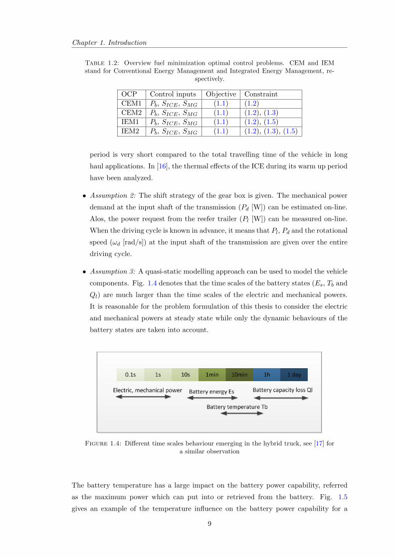
• Assumption 3: A quasi-static modelling approach can be used to model the vehicle
components. Fig. 1.4 denotes that the time scales of the battery states (Es, Tb and
Ql) are much larger than the time scales of the electric and mechanical powers.
It is reasonable for the problem formulation of this thesis to consider the electric
and mechanical powers at steady state while only the dynamic behaviours of the
battery states are taken into account.
Figure 1.4: Different time scales behaviour emerging in the hybrid truck, see [17] fora similar observation
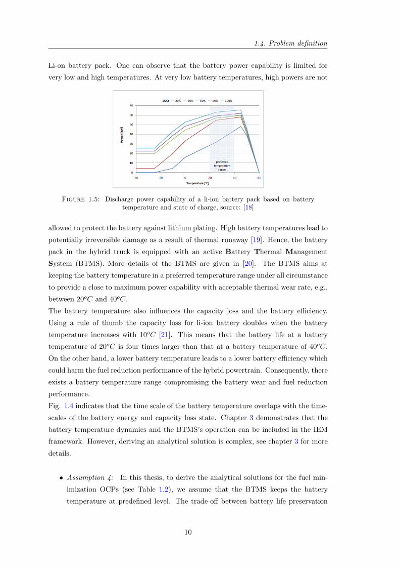
The battery temperature has a large impact on the battery power capability, referred
as the maximum power which can put into or retrieved from the battery. Fig. 1.5
gives an example of the temperature influence on the battery power capability for a
9
1.4. Problem definition
Li-on battery pack. One can observe that the battery power capability is limited for
very low and high temperatures. At very low battery temperatures, high powers are not
Figure 1.5: Discharge power capability of a li-ion battery pack based on batterytemperature and state of charge, source: [18]
allowed to protect the battery against lithium plating. High battery temperatures lead to
potentially irreversible damage as a result of thermal runaway [19]. Hence, the battery
pack in the hybrid truck is equipped with an active Battery Thermal Management
System (BTMS). More details of the BTMS are given in [20]. The BTMS aims at
keeping the battery temperature in a preferred temperature range under all circumstance
to provide a close to maximum power capability with acceptable thermal wear rate, e.g.,
between 20oC and 40oC.
The battery temperature also influences the capacity loss and the battery efficiency.
Using a rule of thumb the capacity loss for li-ion battery doubles when the battery
temperature increases with 10oC [21]. This means that the battery life at a battery
temperature of 20oC is four times larger than that at a battery temperature of 40oC.
On the other hand, a lower battery temperature leads to a lower battery efficiency which
could harm the fuel reduction performance of the hybrid powertrain. Consequently, there
exists a battery temperature range compromising the battery wear and fuel reduction
performance.
Fig. 1.4 indicates that the time scale of the battery temperature overlaps with the time-
scales of the battery energy and capacity loss state. Chapter 3 demonstrates that the
battery temperature dynamics and the BTMS’s operation can be included in the IEM
framework. However, deriving an analytical solution is complex, see chapter 3 for more
details.
• Assumption 4: In this thesis, to derive the analytical solutions for the fuel min-
imization OCPs (see Table 1.2), we assume that the BTMS keeps the battery
temperature at predefined level. The trade-off between battery life preservation
10
Chapter 1. Introduction
and fuel reduction performance will be analyzed for different battery temperature
levels.
The necessity of these assumptions becomes clear in the next chapters.
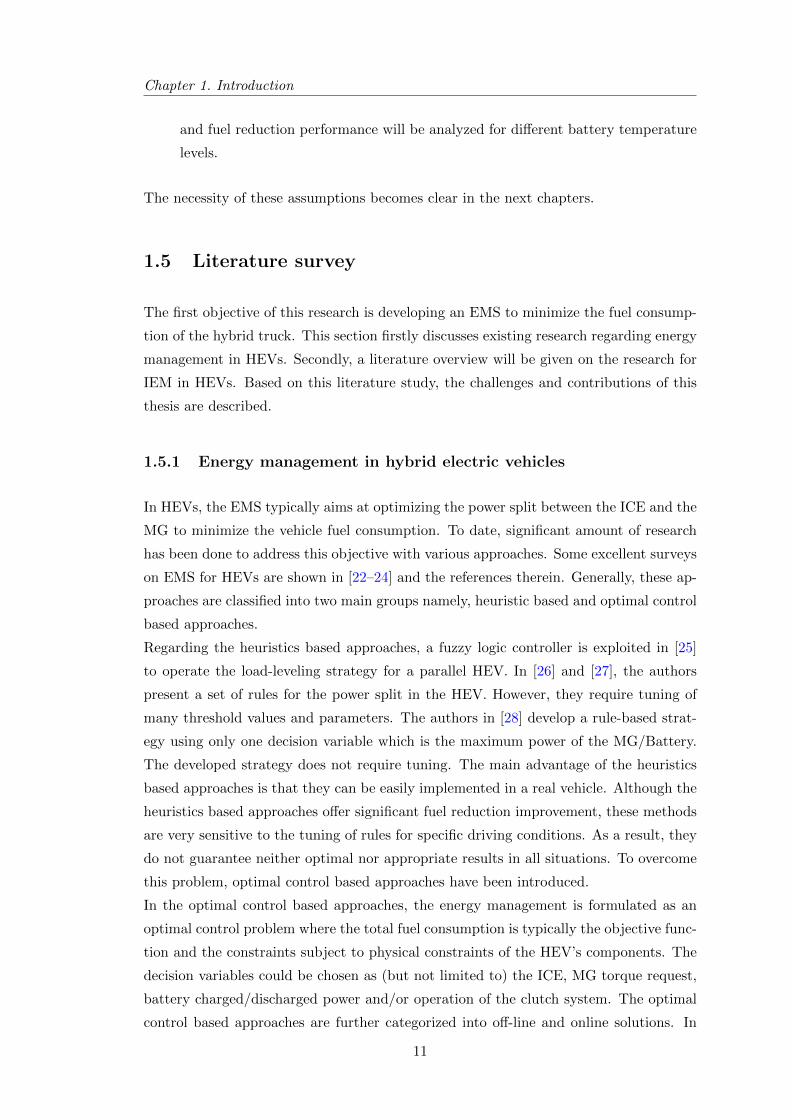
1.5 Literature survey
The first objective of this research is developing an EMS to minimize the fuel consump-
tion of the hybrid truck. This section firstly discusses existing research regarding energy
management in HEVs. Secondly, a literature overview will be given on the research for
IEM in HEVs. Based on this literature study, the challenges and contributions of this
thesis are described.
1.5.1 Energy management in hybrid electric vehicles
In HEVs, the EMS typically aims at optimizing the power split between the ICE and the
MG to minimize the vehicle fuel consumption. To date, significant amount of research
has been done to address this objective with various approaches. Some excellent surveys
on EMS for HEVs are shown in [22–24] and the references therein. Generally, these ap-
proaches are classified into two main groups namely, heuristic based and optimal control
based approaches.
Regarding the heuristics based approaches, a fuzzy logic controller is exploited in [25]
to operate the load-leveling strategy for a parallel HEV. In [26] and [27], the authors
present a set of rules for the power split in the HEV. However, they require tuning of
many threshold values and parameters. The authors in [28] develop a rule-based strat-
egy using only one decision variable which is the maximum power of the MG/Battery.
The developed strategy does not require tuning. The main advantage of the heuristics
based approaches is that they can be easily implemented in a real vehicle. Although the
heuristics based approaches offer significant fuel reduction improvement, these methods
are very sensitive to the tuning of rules for specific driving conditions. As a result, they
do not guarantee neither optimal nor appropriate results in all situations. To overcome
this problem, optimal control based approaches have been introduced.
In the optimal control based approaches, the energy management is formulated as an
optimal control problem where the total fuel consumption is typically the objective func-
tion and the constraints subject to physical constraints of the HEV’s components. The
decision variables could be chosen as (but not limited to) the ICE, MG torque request,
battery charged/discharged power and/or operation of the clutch system. The optimal
control based approaches are further categorized into off-line and online solutions. In
11
1.5. Literature survey
the off-line solutions, the driving cycle is known and predefined. The optimal solution
is found by utilizing various techniques as linear programming [29], quadratic program-
ming [30] and Dynamic Programming [31–33]. The obtained optimal solutions can be
exploited as a bench-mark to evaluate other EMSs. Moreover, they also assist in deter-
mining the rules for developing the rule-based strategies [34].
Regarding the on-line strategies, besides various non-linear control strategies [35], [36],
the Equivalent fuel Consumption Management Strategy (ECMS) has shown to be one
of the best performing strategies with respect to fuel reduction performance [35]. A
large amount of research has been reported in utilizing the ECMS technique for EMS,
part of them are listed as [15, 23, 35, 37–43]. Experiments on real vehicles [44], [45]
for these EMSs demonstrate a very promising performance and robustness in reducing
fuel consumption and the associated CO2 emission. In [46], a model of the GM Voltec
powertrain is implemented as a simulator to evaluate various heuristics and ECMS based
EMSs. The simulation results show that the ECMS based EMSs generally outperform
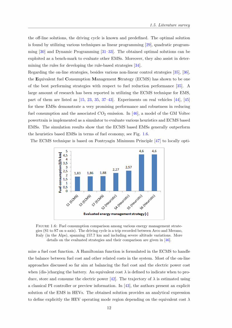
the heuristics based EMSs in terms of fuel economy, see Fig. 1.6.
The ECMS technique is based on Pontryagin Minimum Principle [47] to locally opti-
Figure 1.6: Fuel consumption comparison among various energy management strate-gies (S1 to S7 on x-axis). The driving cycle is a trip recorded between Arco and Merano,Italy (in the Alps), spanning 157.7 km and including severe altitude variations. More
details on the evaluated strategies and their comparison are given in [46].
mize a fuel cost function. A Hamiltonian function is formulated in the ECMS to handle
the balance between fuel cost and other related costs in the system. Most of the on-line
approaches discussed so far aim at balancing the fuel cost and the electric power cost
when (dis-)charging the battery. An equivalent cost λ is defined to indicate when to pro-
duce, store and consume the electric power [42]. The trajectory of λ is estimated using
a classical PI controller or preview information. In [43], the authors present an explicit
solution of the EMS in HEVs. The obtained solution provides an analytical expression
to define explicitly the HEV operating mode region depending on the equivalent cost λ
12
Chapter 1. Introduction
(or s as denoted in [43]) and the power demand from the drivetrain.
Contribution of this thesis to energy management in HEVs
Most of the aforementioned approaches study an HEV with only one clutch between the
ICE and the drivetrain. The benefit from decoupling the MG from the drivetrain has
not been explored. This research extends existing solutions by providing an analytical
solution to the EMS where the benefit from also using the MG clutch is demonstrated.
1.5.2 Integrated Energy Management in hybrid electric vehicles
Besides the ICE and battery, there exist other energy buffers and energy sources from
other components [48]. As suggested in [49], taking into account additional systems can
further improve the system efficiency. In [50], [16], the ICE temperature is incorporated
in addition to the battery energy state to optimally control the HEV to minimize the fuel
consumption during the ICE warmup. The authors in [16] show that the optimization
can also be solved explicitly as an extension of the optimal control solution in [43]. In
[51], the concept of Integrated Powertrain Control (IPC) is proposed to incorporate the
system states from the powertrain components and the aftertreatment system. Specifi-
cally, the conventional ECMS [42] is extended to take into account the battery energy
state, Selective Catalytic Reduction (SCR) catalyst temperature state and the tail-pipe
NOx emissions to minimize the operational cost and satisfy the pollutant constraint.
The IPC concept is also presented in [52] for an application of an Euro-VI diesel engine
with a Waste Heat Recovery system. The Diesel Oxidation Catalyst (DOC) catalyst
temperature, SCR temperature and the NOx tail-pipe emission are incorporated in the
control strategy. The control inputs are then determined to minimize the fuel consump-
tion within the constraints set by the emission legislation. In [53], the authors show via
simulation the trade-off between the cost of the BTMS action versus the benefit from
the hybrid powertrain. This trade-off is also discussed in [54], [20] where an Integrated
Energy and battery Thermal Management (IETM) is introduced to balance the costs
among fuel consumption, electric power from (dis-)charging the battery and fuel con-
sumed by the BTMS.
In an HEV, the total tail-pipe emission has to comply with the emission legislation.
On the other hand, the battery life needs to be sufficient to make the HEV commercial
profitable. The issue of battery wear in commercial vehicles is recognized for plug-in
HEVs in [13]. In hybrid electric trucks, the balance among fuel consumption reduction,
battery cost and battery life should also be taken into account [14].
Integrating battery wear in EMSs
In recent years, integration of battery wear into the EMS framework of the HEVs has
13
1.5. Literature survey
become a viable research topic. In [55], the authors demonstrate the necessity to incor-
porate battery wear into the optimal powertrain sizing and control via an example of a
series hybrid electric bus. In [56], an LPV approach is presented to minimize the vehicle
fuel consumption by forcing the battery state of charge tracking a predefined proper ref-
erence trajectory. It is observed from simulation results in [56] that when degradation
of battery capacity occurs, the battery energy should be used less to prolong the battery
life. In [57], a soft constraint is set on the battery cell temperature to prevent indirectly
the battery from its fast-aging region. However, in both [56] and [57], the battery wear is
not explicitly taken into account in the problem formulation. The compromise between
battery life preservation and fuel consumption reduction is not shown in both [56] and
[57]. This trade-off is discussed in [58–63] where the authors exploit their developed
battery wear models to quantify the battery wear in the framework of the EMS.
The developed strategies in [58–63] make use of the ECMS technique [37], [23] to op-
timize the power/torque split between the ICE and the MG. In [58] battery wear is
incorporated directly in the objective function with a tuned weighting factor, and the
Hamiltonian function takes into account the fuel, electric power and battery wear cost.
Similarly, the authors in [60] and [62] weight the battery wear in the objective function,
but the Hamiltonian function is extended to take into account the cost from the energy
request to heat up/cool down the battery temperature. Minimization of the Hamilto-
nian function in [58, 60, 62] is not shown explicitly. Moreover, the weighting factors in
[58, 60, 62] are arbitrary values and have to be manually adjusted to satisfy the battery
life requirement with the assumption that the driving cycle is known in advance. Hence,
the developed strategies in [58, 60, 62] are not strictly causal. In [61], [63], to preserve
the battery life, an adaptive factor is introduced to artificially increase the battery power
loss in the Hamiltonian function to restrict the battery usage when necessary. The au-
thors in [59], on the other hand, extend the Hamiltonian function to balance three costs:
fuel consumption, electric power and battery wear. However, an analytical solution for
minimization of the Hamiltonian function is not derived. The developed strategy in
[59] is causal. It utilizes two feedback loops to estimate the control parameters on-line.
These feedback loops keep the battery state of charge and state of health around their
predefined reference trajectories. The benefit of utilizing feedforward control to estimate
the control parameters was not explored in [59]. And, an appropriate selection of refer-
ence trajectory for the battery state of health had not been discussed in [59].
Contributions of this thesis to integrated energy and battery life management
This thesis contributes to finding an analytical solution to the Integrated Energy and
Battery Life Management. An analytical solution provides fundamental understanding
for both mathematical and physical insight of the optimal control problem [64]. The
obtained analytical solution reveals that in the EMS framework, the battery life is pre-
served by not (dis-)charging the battery at peak powers to avoid fast deterioration of
14
Chapter 1. Introduction
Table 1.3: Comparison of developed Integrated Energy and Battery Life Managementstrategies in this thesis with existing literature. Objective function OF1 refers to thefuel minimization. Objective function OF2 refers to minimizing the summation of fuel
consumption and battery wear with a weighting factor.
References IEM A-IEM[58] [59] [60] [57] [56] [62] [61] [63] (Thesis) (Thesis)
Year 2011 2012 2013 2013 2013 2014 2014 2014 2015 2015Objective OF1 - + - + + - + + + +function OF2 + - + - - + - - - -Constraints Es + + + + + + + + + +on system Ql + + + - - + + + + +states Tb - - + + - + + - - -
SolutionNumerical + + + + + + + + - -Analytical - - - - - - - - + +
Causal Feedback - + - - - - - + - +solution Feedback +
- - - - - - - + - +FeedforwardAppropriate
- - - +referencetrajectory
the battery wear.
Having the analytical solutions for energy management in the hybrid truck as the off-
line solutions, this thesis also develops a adaptive real-time implementable IEM (A-IEM)
strategy to minimize the hybrid truck fuel consumption while meeting the battery life
requirement. We explore the combination of feedforward and feedback control to obtain
appropriate control parameters. Combination of feedforward and feedback control re-
sults in a reliable solution for satisfying the constraints while achieving almost minimal
fuel consumption. In the thesis, the reference trajectory for the battery capacity loss
state is constructed based on the physical characteristic of the battery wear over the
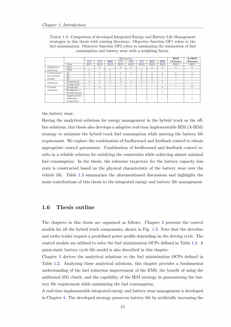
vehicle life. Table 1.3 summarizes the aforementioned discussions and highlights the
main contributions of this thesis to the integrated energy and battery life management.
1.6 Thesis outline
The chapters in this thesis are organized as follows. Chapter 2 presents the control
models for all the hybrid truck components, shown in Fig. 1.3. Note that the driveline
and reefer trailer request a predefined power profile depending on the driving cycle. The
control models are utilized to solve the fuel minimization OCPs defined in Table 1.2. A
quasi-static battery cycle life model is also described in this chapter.
Chapter 3 derives the analytical solutions to the fuel minimization OCPs defined in
Table 1.2. Analyzing these analytical solutions, this chapter provides a fundamental
understanding of the fuel reduction improvement of the EMS, the benefit of using the
additional MG clutch, and the capability of the IEM strategy in guaranteeing the bat-
tery life requirement while minimizing the fuel consumption.
A real-time implementable integrated energy and battery wear management is developed
in Chapter 4. The developed strategy preserves battery life by artificially increasing the
15
1.6. Thesis outline
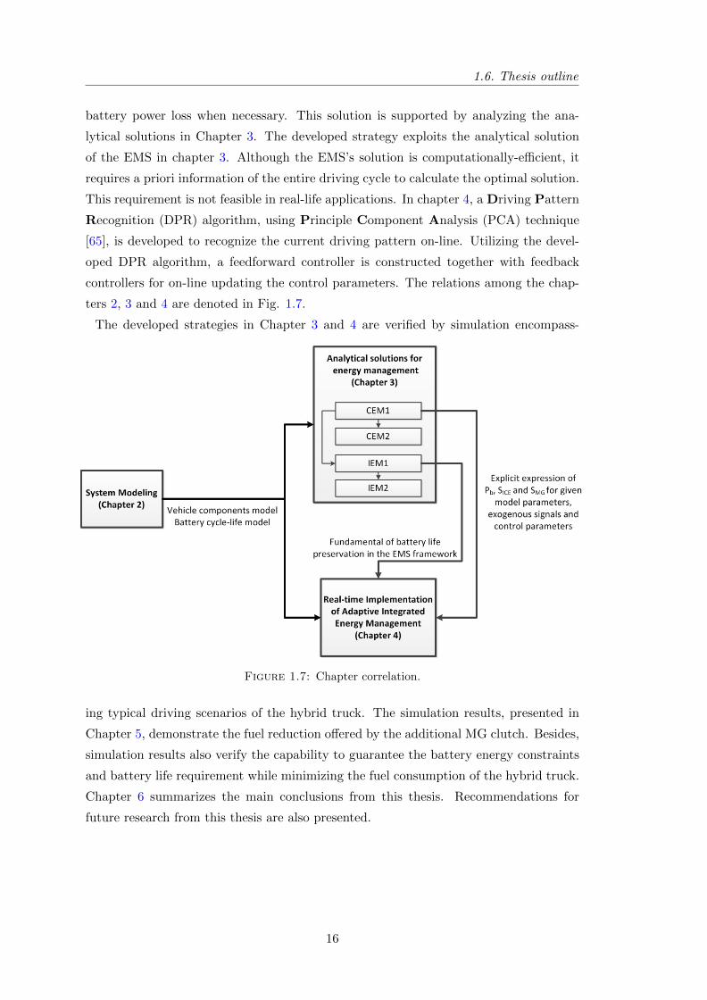
battery power loss when necessary. This solution is supported by analyzing the ana-
lytical solutions in Chapter 3. The developed strategy exploits the analytical solution
of the EMS in chapter 3. Although the EMS’s solution is computationally-efficient, it
requires a priori information of the entire driving cycle to calculate the optimal solution.
This requirement is not feasible in real-life applications. In chapter 4, a Driving Pattern
Recognition (DPR) algorithm, using Principle Component Analysis (PCA) technique
[65], is developed to recognize the current driving pattern on-line. Utilizing the devel-
oped DPR algorithm, a feedforward controller is constructed together with feedback
controllers for on-line updating the control parameters. The relations among the chap-
ters 2, 3 and 4 are denoted in Fig. 1.7.
The developed strategies in Chapter 3 and 4 are verified by simulation encompass-
Figure 1.7: Chapter correlation.
ing typical driving scenarios of the hybrid truck. The simulation results, presented in
Chapter 5, demonstrate the fuel reduction offered by the additional MG clutch. Besides,
simulation results also verify the capability to guarantee the battery energy constraints
and battery life requirement while minimizing the fuel consumption of the hybrid truck.
Chapter 6 summarizes the main conclusions from this thesis. Recommendations for
future research from this thesis are also presented.
16
Chapter 2
System modeling
This chapter presents the vehicle model and the component models needed for solving
the fuel minimization OCPs defined in Table 1.2.
2.1 Vehicle model
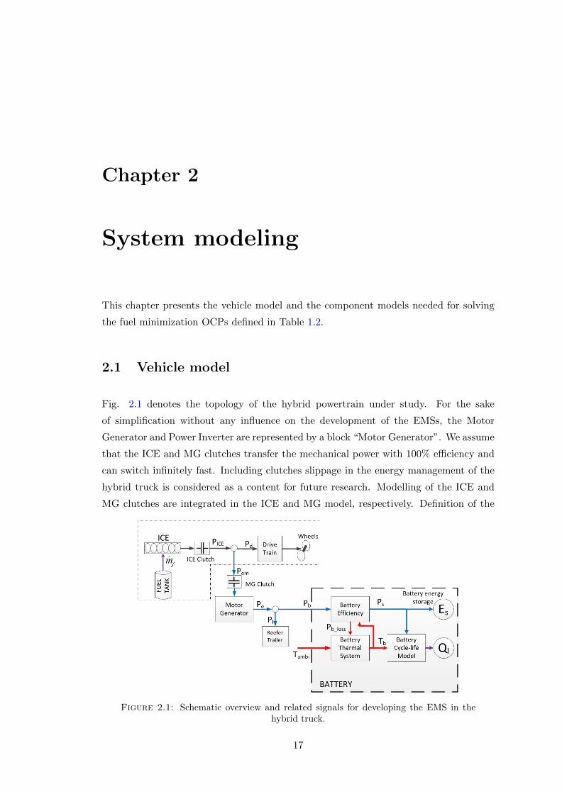
Fig. 2.1 denotes the topology of the hybrid powertrain under study. For the sake
of simplification without any influence on the development of the EMSs, the Motor
Generator and Power Inverter are represented by a block “Motor Generator”. We assume
that the ICE and MG clutches transfer the mechanical power with 100% efficiency and
can switch infinitely fast. Including clutches slippage in the energy management of the
hybrid truck is considered as a content for future research. Modelling of the ICE and
MG clutches are integrated in the ICE and MG model, respectively. Definition of the
Figure 2.1: Schematic overview and related signals for developing the EMS in thehybrid truck.
17
2.1. Vehicle model
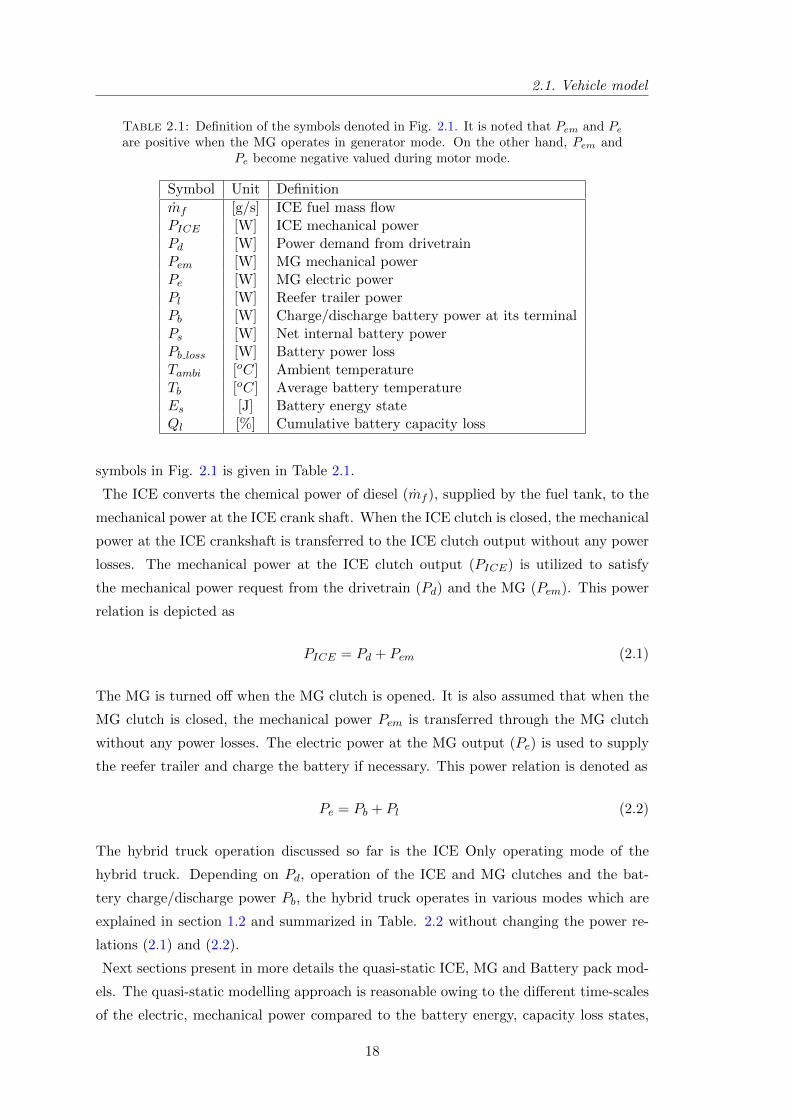
Table 2.1: Definition of the symbols denoted in Fig. 2.1. It is noted that Pem and Peare positive when the MG operates in generator mode. On the other hand, Pem and
Pe become negative valued during motor mode.
Symbol Unit Definition
mf [g/s] ICE fuel mass flowPICE [W] ICE mechanical powerPd [W] Power demand from drivetrainPem [W] MG mechanical powerPe [W] MG electric powerPl [W] Reefer trailer powerPb [W] Charge/discharge battery power at its terminalPs [W] Net internal battery powerPb loss [W] Battery power lossTambi [oC] Ambient temperatureTb [oC] Average battery temperatureEs [J] Battery energy stateQl [%] Cumulative battery capacity loss
symbols in Fig. 2.1 is given in Table 2.1.
The ICE converts the chemical power of diesel (mf ), supplied by the fuel tank, to the
mechanical power at the ICE crank shaft. When the ICE clutch is closed, the mechanical
power at the ICE crankshaft is transferred to the ICE clutch output without any power
losses. The mechanical power at the ICE clutch output (PICE) is utilized to satisfy
the mechanical power request from the drivetrain (Pd) and the MG (Pem). This power
relation is depicted as
PICE = Pd + Pem (2.1)
The MG is turned off when the MG clutch is opened. It is also assumed that when the
MG clutch is closed, the mechanical power Pem is transferred through the MG clutch
without any power losses. The electric power at the MG output (Pe) is used to supply
the reefer trailer and charge the battery if necessary. This power relation is denoted as
Pe = Pb + Pl (2.2)
The hybrid truck operation discussed so far is the ICE Only operating mode of the
hybrid truck. Depending on Pd, operation of the ICE and MG clutches and the bat-
tery charge/discharge power Pb, the hybrid truck operates in various modes which are
explained in section 1.2 and summarized in Table. 2.2 without changing the power re-
lations (2.1) and (2.2).
Next sections present in more details the quasi-static ICE, MG and Battery pack mod-
els. The quasi-static modelling approach is reasonable owing to the different time-scales
of the electric, mechanical power compared to the battery energy, capacity loss states,
18
Chapter 2. System modeling
Table 2.2: Hybrid truck operating mode. ‘+’ and ‘-’ correspond to the positive andnegative value. The positive values of Pd imply the driving periods whereas the negativevalues of Pd refer to the braking periods. The positive values of Pb mean the battery ischarged while the negative values of Pb denote the operation of discharging the battery.
Operating mode Pd SICE SMG PbPSM + 1 0 -MO + 0 1 -ICE Only + 1 1 0MA + 1 1 -C + 1 1 +R - 1 1 +
see also Fig. 1.4. Modeling of the reefer trailer and the drivetrain are neglected due
to the assumption that the reefer trailer power request Pl and the mechanical power
demand Pd at the transmission side of the drivetrain can be estimated on-line.
2.2 Internal combustion engine model
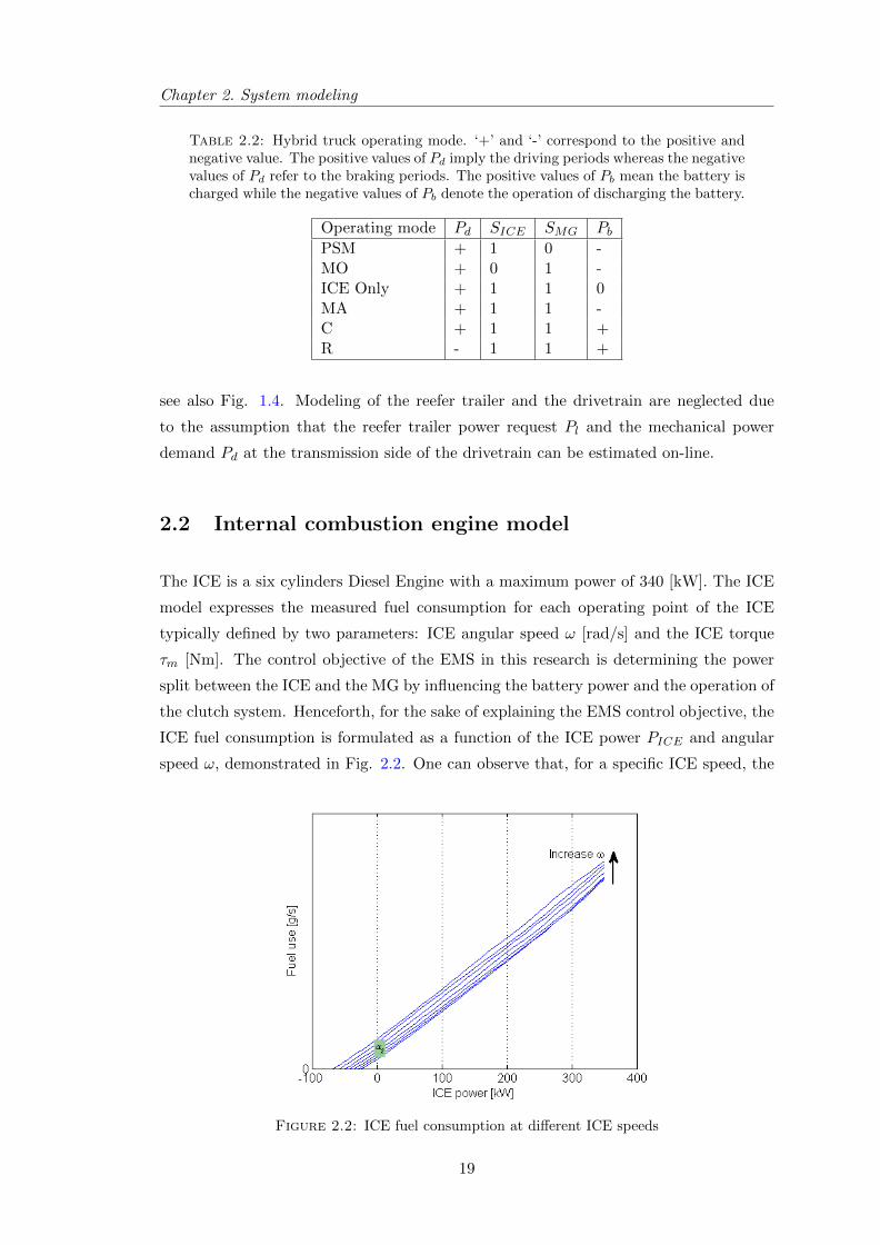
The ICE is a six cylinders Diesel Engine with a maximum power of 340 [kW]. The ICE
model expresses the measured fuel consumption for each operating point of the ICE
typically defined by two parameters: ICE angular speed ω [rad/s] and the ICE torque
τm [Nm]. The control objective of the EMS in this research is determining the power
split between the ICE and the MG by influencing the battery power and the operation of
the clutch system. Henceforth, for the sake of explaining the EMS control objective, the
ICE fuel consumption is formulated as a function of the ICE power PICE and angular
speed ω, demonstrated in Fig. 2.2. One can observe that, for a specific ICE speed, the
Figure 2.2: ICE fuel consumption at different ICE speeds
19
2.2. Internal combustion engine model
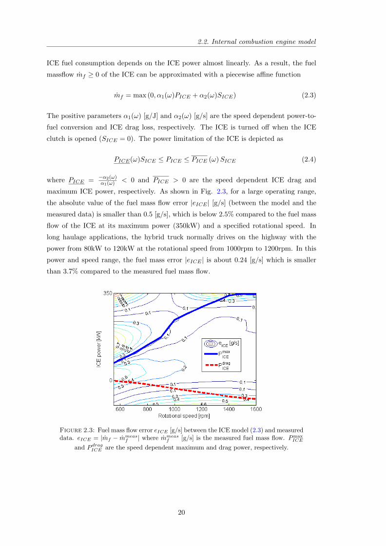
ICE fuel consumption depends on the ICE power almost linearly. As a result, the fuel
massflow mf ≥ 0 of the ICE can be approximated with a piecewise affine function
mf = max (0, α1(ω)PICE + α2(ω)SICE) (2.3)
The positive parameters α1(ω) [g/J] and α2(ω) [g/s] are the speed dependent power-to-
fuel conversion and ICE drag loss, respectively. The ICE is turned off when the ICE
clutch is opened (SICE = 0). The power limitation of the ICE is depicted as
PICE(ω)SICE ≤ PICE ≤ PICE (ω)SICE (2.4)
where PICE = −α2(ω)α1(ω) < 0 and PICE > 0 are the speed dependent ICE drag and
maximum ICE power, respectively. As shown in Fig. 2.3, for a large operating range,
the absolute value of the fuel mass flow error |eICE | [g/s] (between the model and the
measured data) is smaller than 0.5 [g/s], which is below 2.5% compared to the fuel mass
flow of the ICE at its maximum power (350kW) and a specified rotational speed. In
long haulage applications, the hybrid truck normally drives on the highway with the
power from 80kW to 120kW at the rotational speed from 1000rpm to 1200rpm. In this
power and speed range, the fuel mass error |eICE | is about 0.24 [g/s] which is smaller
than 3.7% compared to the measured fuel mass flow.
Figure 2.3: Fuel mass flow error eICE [g/s] between the ICE model (2.3) and measureddata. eICE = |mf − mmeas
f | where mmeasf [g/s] is the measured fuel mass flow. Pmax
ICE
and P dragICE are the speed dependent maximum and drag power, respectively.
20
Chapter 2. System modeling
2.3 Motor generator model
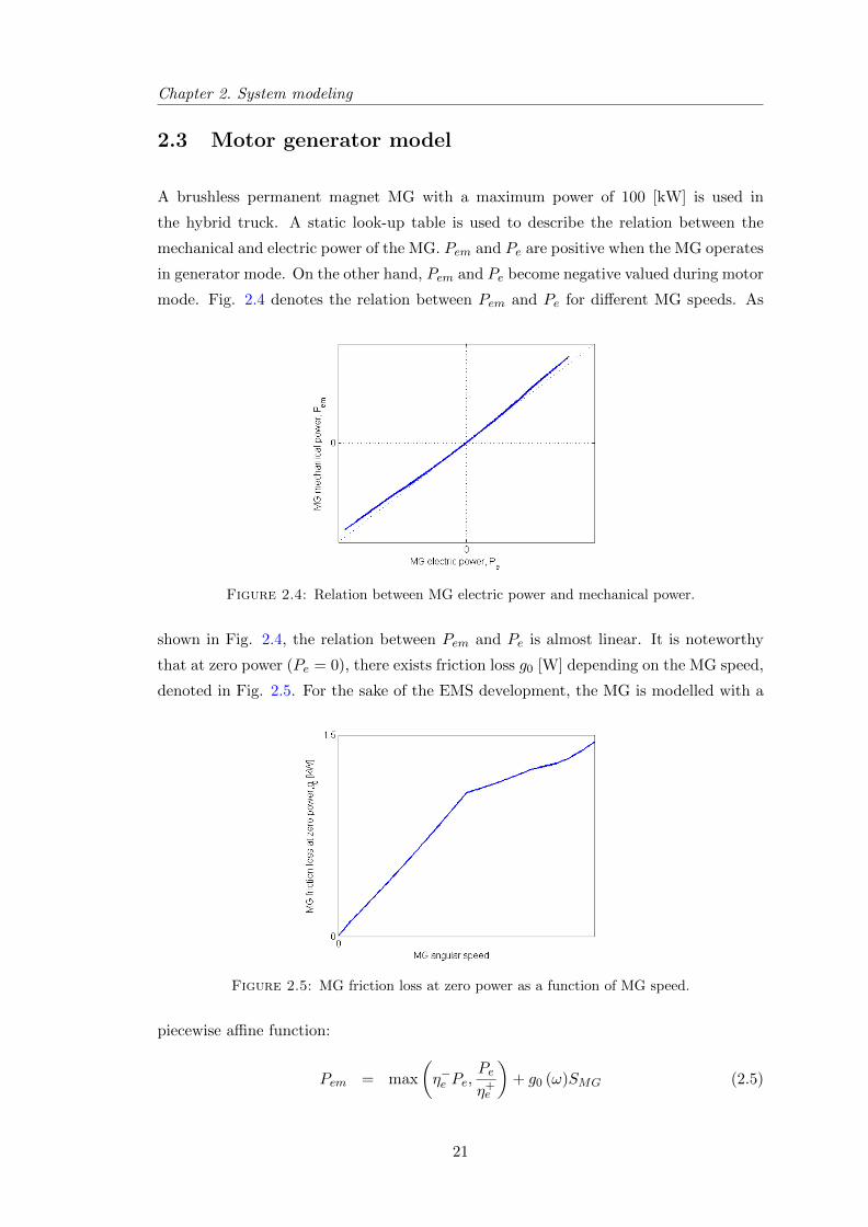
A brushless permanent magnet MG with a maximum power of 100 [kW] is used in
the hybrid truck. A static look-up table is used to describe the relation between the
mechanical and electric power of the MG. Pem and Pe are positive when the MG operates
in generator mode. On the other hand, Pem and Pe become negative valued during motor
mode. Fig. 2.4 denotes the relation between Pem and Pe for different MG speeds. As
Figure 2.4: Relation between MG electric power and mechanical power.
shown in Fig. 2.4, the relation between Pem and Pe is almost linear. It is noteworthy
that at zero power (Pe = 0), there exists friction loss g0 [W] depending on the MG speed,
denoted in Fig. 2.5. For the sake of the EMS development, the MG is modelled with a
Figure 2.5: MG friction loss at zero power as a function of MG speed.
piecewise affine function:
Pem = max
(η−e Pe,
Pe
η+e
)+ g0 (ω)SMG (2.5)
21
2.3. Motor generator model
where η−e and η+e are the power conversion efficiencies (including also the Power Inverter
efficiency) in Motor and Generator mode, respectively. The power limitation of the MG
is denoted as
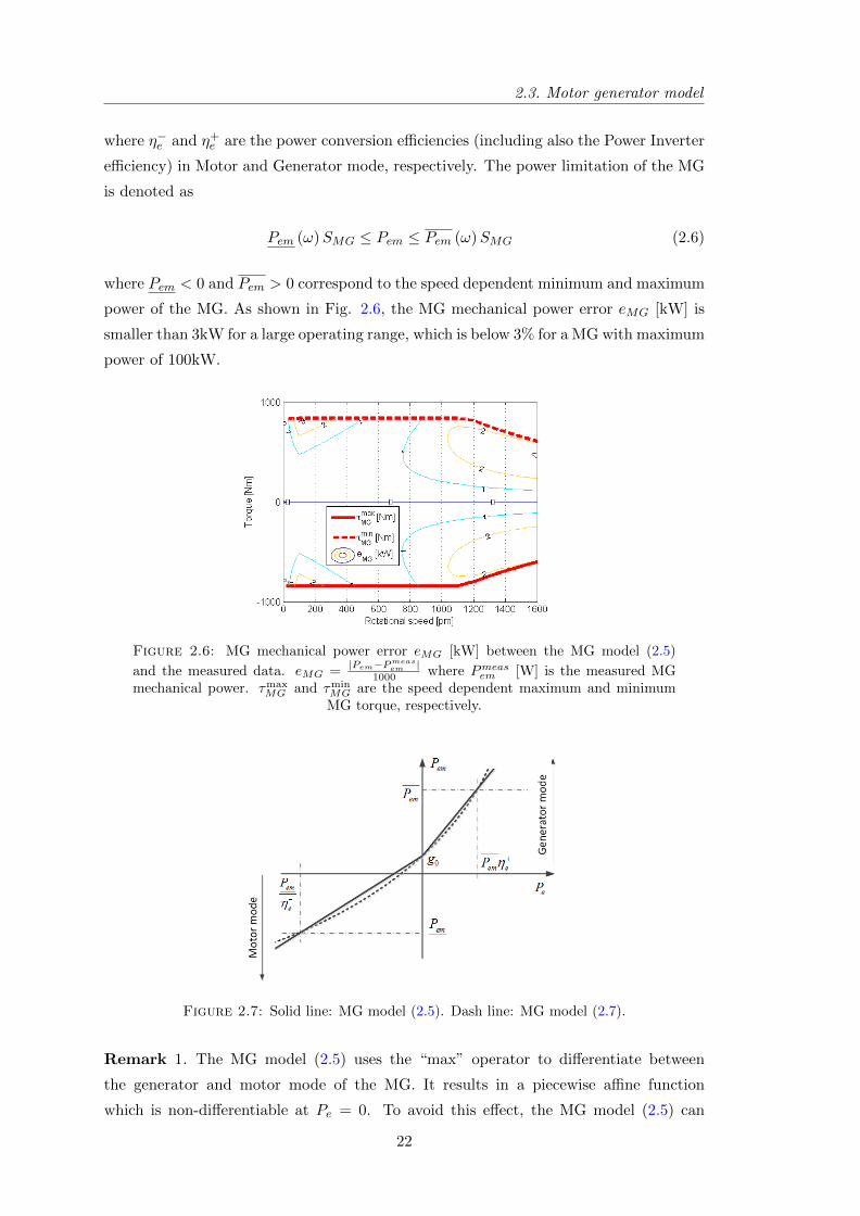
Pem (ω)SMG ≤ Pem ≤ Pem (ω)SMG (2.6)
where Pem < 0 and Pem > 0 correspond to the speed dependent minimum and maximum
power of the MG. As shown in Fig. 2.6, the MG mechanical power error eMG [kW] is
smaller than 3kW for a large operating range, which is below 3% for a MG with maximum
power of 100kW.
Figure 2.6: MG mechanical power error eMG [kW] between the MG model (2.5)
and the measured data. eMG =|Pem−Pmeas
em |1000 where Pmeasem [W] is the measured MG
mechanical power. τmaxMG and τmin
MG are the speed dependent maximum and minimumMG torque, respectively.
Figure 2.7: Solid line: MG model (2.5). Dash line: MG model (2.7).
Remark 1. The MG model (2.5) uses the “max” operator to differentiate between
the generator and motor mode of the MG. It results in a piecewise affine function
which is non-differentiable at Pe = 0. To avoid this effect, the MG model (2.5) can
22
Chapter 2. System modeling
be approximated by a quadratic function with respect to Pe,
Pem = η1P2e + η2Pe + g0(ω)SMG (2.7)
where η1 and η2 are estimated by fitting (2.7) to the three points(Pem
η−e, Pem
), (0, g0) and(
Pemη+e , Pem
), see Fig. 2.7. The advantage and disadvantage of using the MG model
(2.7) will be discussed in chapter 3.
2.4 Battery model
The hybrid truck is equipped with a li-ion battery pack with a peak power of 120
[kW]. The battery model consists of the battery efficiency, battery thermal system and
battery cycle-life model, see Fig. 2.1. This thesis does not aim at integrating the
battery temperature and operation of the BTMS in the energy management. Henceforth,
modeling of the battery thermal system is not presented here. In [20], more details of
the battery thermal system are given.
2.4.1 Battery efficiency model
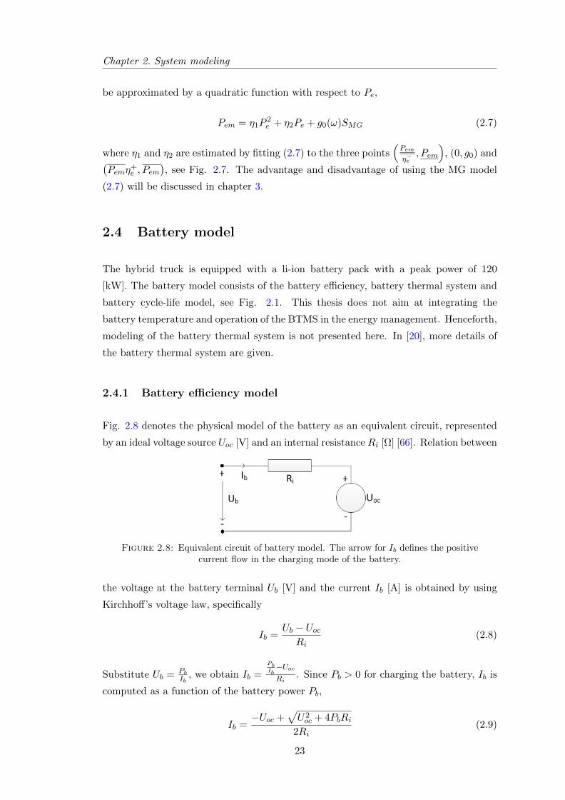
Fig. 2.8 denotes the physical model of the battery as an equivalent circuit, represented
by an ideal voltage source Uoc [V] and an internal resistance Ri [Ω] [66]. Relation between
Figure 2.8: Equivalent circuit of battery model. The arrow for Ib defines the positivecurrent flow in the charging mode of the battery.
the voltage at the battery terminal Ub [V] and the current Ib [A] is obtained by using
Kirchhoff’s voltage law, specifically
Ib =Ub − Uoc
Ri(2.8)
Substitute Ub = PbIb
, we obtain Ib =PbIb−UocRi
. Since Pb > 0 for charging the battery, Ib is
computed as a function of the battery power Pb,
Ib =−Uoc +
√U2oc + 4PbRi
2Ri(2.9)
23
2.4. Battery model
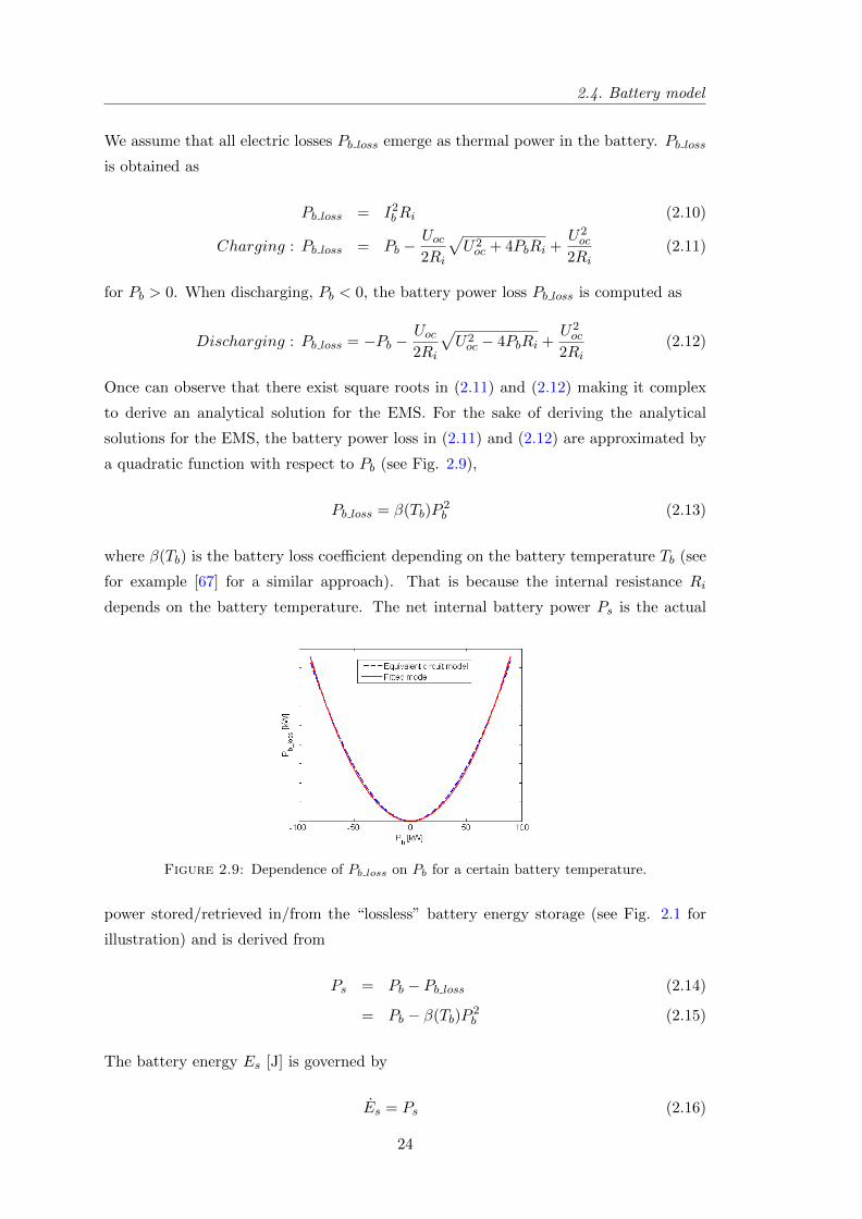
We assume that all electric losses Pb loss emerge as thermal power in the battery. Pb loss
is obtained as
Pb loss = I2bRi (2.10)
Charging : Pb loss = Pb −Uoc2Ri
√U2oc + 4PbRi +
U2oc
2Ri(2.11)
for Pb > 0. When discharging, Pb < 0, the battery power loss Pb loss is computed as
Discharging : Pb loss = −Pb −Uoc2Ri
√U2oc − 4PbRi +
U2oc
2Ri(2.12)
Once can observe that there exist square roots in (2.11) and (2.12) making it complex
to derive an analytical solution for the EMS. For the sake of deriving the analytical
solutions for the EMS, the battery power loss in (2.11) and (2.12) are approximated by
a quadratic function with respect to Pb (see Fig. 2.9),
Pb loss = β(Tb)P2b (2.13)
where β(Tb) is the battery loss coefficient depending on the battery temperature Tb (see
for example [67] for a similar approach). That is because the internal resistance Ri
depends on the battery temperature. The net internal battery power Ps is the actual
Figure 2.9: Dependence of Pb loss on Pb for a certain battery temperature.
power stored/retrieved in/from the “lossless” battery energy storage (see Fig. 2.1 for
illustration) and is derived from
Ps = Pb − Pb loss (2.14)
= Pb − β(Tb)P2b (2.15)
The battery energy Es [J] is governed by
Es = Ps (2.16)
24
Chapter 2. System modeling
The power limitation of the battery is depicted as
Pb ≤ Pb ≤ Pb (2.17)
with
Pb = min(Pbd, SOFcha(Es, Tb)
)Pb = max
(Pbd,−SOFdis(Es, Tb)
)SOFdis > 0 [W] and SOFcha > 0 [W] represent the power capability for (dis-) charging
the battery as function of Es and Tb [18]. Pbd > 0 [W] and Pbd < 0 [W] are the battery
power limitations incorporating the power limitations of the ICE, MG and the capability
to supply the power demand Pd as well as the reefer trailer power request Pl, specifically
Pbd = max[(
min(PICE − Pd, Pem
)− g0
)η+e − Pl, 0
]Pbd = min
[max
(PICE − Pd, Pem
)− g0
η−e− Pl, 0
]
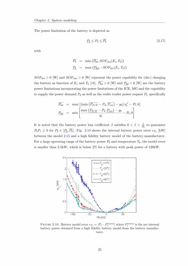
It is noted that the battery power loss coefficient β satisfies 0 < β < 1Pb
to guarantee
PbPs ≥ 0 for Pb ∈ [Pb, Pb]. Fig. 2.10 shows the internal battery power error ePs [kW]
between the model 2.15 and a high fidelity battery model of the battery manufacturer.
For a large operating range of the battery power Pb and temperature Tb, the model error
is smaller than 2.5kW, which is below 2% for a battery with peak power of 120kW.
Figure 2.10: Battery model error ePs= |Ps−Pmanus | where Pmanus is the net internal
battery power obtained from a high fidelity battery model from the battery manufac-turer.
25
2.4. Battery model
2.4.2 Quasi-static battery cycle-life model
This thesis develops a model-based IEM strategy to guarantee the requested battery life
whilst minimizing the vehicle’s fuel consumption. As a result, a battery life model is
necessary. This model should fit the EMS framework. It estimates the battery capacity
loss every time instant when the battery is charged/discharged.
Battery aging, in general, is effected by its calendar-life and cycle-life [68], [69]. While
the calendar-life reflects the degradation of the battery capacity during its storage, the
cycle-life represents the battery capacity reduction when (dis-)charging the battery. The
influences of calendar-life and cycle-life on the total battery capacity loss are normally
assumed to be cumulative [70]. It is, therefore, reasonable to consider their effects on
the battery life separately. The IEM strategy aims at handling the trade-off between
the cost and benefit when (dis-)charging the battery. This paper focuses on the battery
cycle-life.
The Li-ion battery has been widely used in the applications of hybrid and electric ve-
hicles owing to its high energy density and power density [38]. The considered hybrid
truck is also equipped with a Li-ion high-voltage battery pack. In [69], the authors
give an overview on the battery aging mechanism for Li-on battery cells. In [71], the
authors present preliminary results on the effect of battery ageing propagated between
interconnected cells in a battery pack. Battery capacity wears out during its operation
with a rate depending on several factors, e.g., charge/discharge rate, temperature, SOC
level [21].
In [72], the authors investigate a Li-ion battery whose cell technology is similar the one
being used in the considered hybrid truck. A battery cycle-life model for Li-ion battery
cells is empirically constructed from a large amount of experimental data. The cells
were tested at various conditions as combinations of different temperatures, levels of
Depth-of-Discharge (DOD) and constant discharge rates. The model, denoted in (2.18),
describes the dependence of the cumulative battery capacity loss Ql [%] on three factors
namely, battery Ah throughput, C-rate and temperature.
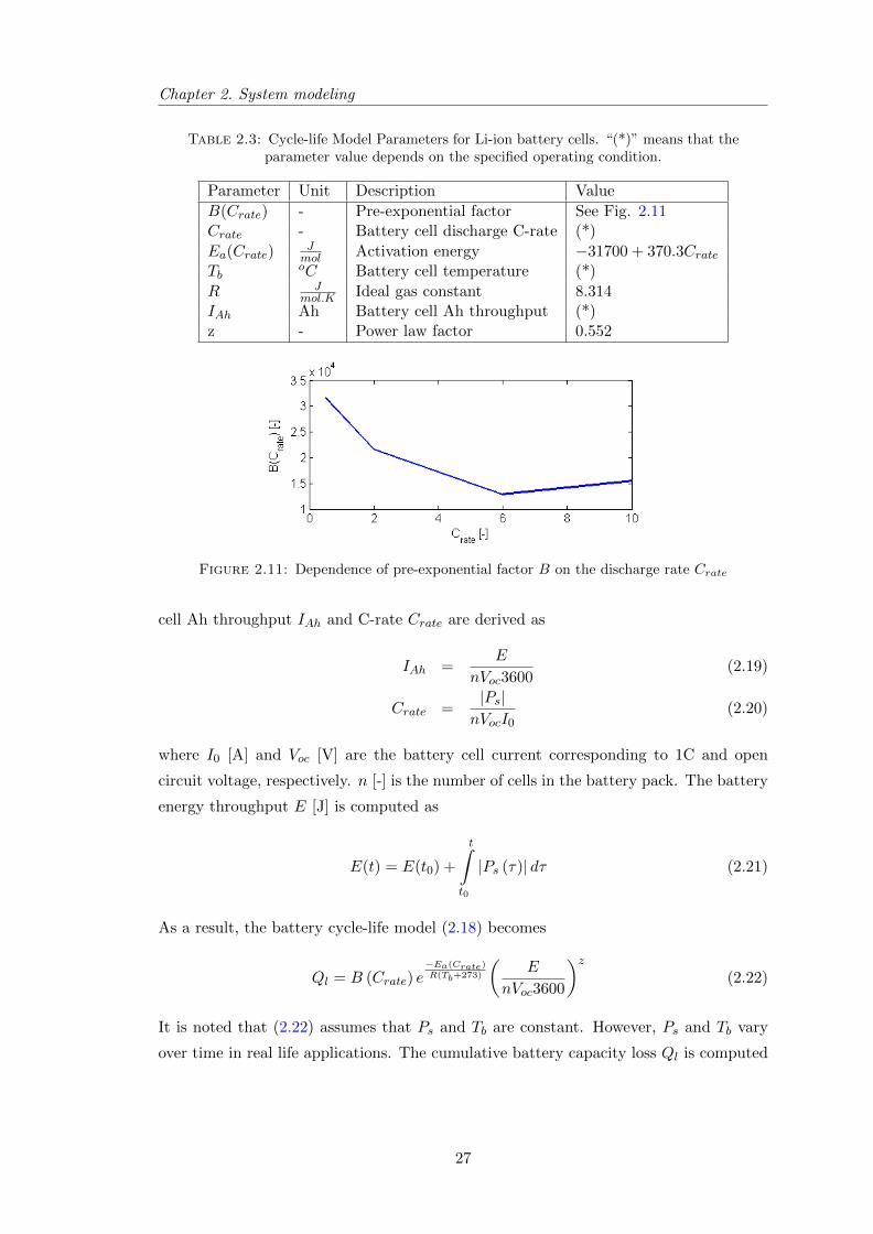
Ql = B(Crate)e−Ea(Crate)R(Tb+273) (IAh)z (2.18)
Table 2.3 gives an overview of the model parameters whose values are given in [72]. The
battery cycle-life model (2.18) estimates the battery capacity loss at cell-level. However,
the considered hybrid truck is equipped with a high voltage battery pack comprising
many cells. Therefore, the model (2.18) is adapted such that the battery cell cycle-life
can be evaluated based on the battery pack power and temperature.
Assume that the battery power is uniformly distributed in the battery pack. The battery
26
Chapter 2. System modeling
Table 2.3: Cycle-life Model Parameters for Li-ion battery cells. “(*)” means that theparameter value depends on the specified operating condition.
Parameter Unit Description Value
B(Crate) - Pre-exponential factor See Fig. 2.11Crate - Battery cell discharge C-rate (*)
Ea(Crate)Jmol Activation energy −31700 + 370.3Crate
TboC Battery cell temperature (*)
R Jmol.K Ideal gas constant 8.314
IAh Ah Battery cell Ah throughput (*)z - Power law factor 0.552
Figure 2.11: Dependence of pre-exponential factor B on the discharge rate Crate
cell Ah throughput IAh and C-rate Crate are derived as
IAh =E
nVoc3600(2.19)
Crate =|Ps|nVocI0
(2.20)
where I0 [A] and Voc [V] are the battery cell current corresponding to 1C and open
circuit voltage, respectively. n [-] is the number of cells in the battery pack. The battery
energy throughput E [J] is computed as
E(t) = E(t0) +
t∫t0
|Ps (τ)| dτ (2.21)
As a result, the battery cycle-life model (2.18) becomes
Ql = B (Crate) e−Ea(Crate)R(Tb+273)
(E
nVoc3600
)z(2.22)
It is noted that (2.22) assumes that Ps and Tb are constant. However, Ps and Tb vary
over time in real life applications. The cumulative battery capacity loss Ql is computed
27

2.4. Battery model
by adding up the incremental capacity loss Ql in the static battery cycle-life model
Ql (t) = Ql (t0) +
t∫t0
Ql (Ps, Tb, τ) dτ (2.23)
To obtain the incremental capacity loss Ql at a certain battery wear status Ql, a quasi-
static approach is utilized since this approach is well suited for the development of the
EMS [38]. The rate of change of Crate and Tb are neglected. Hence, Ql can be derived
from (2.22) as follows,
dQldt
=∂Ql∂E
dE
dt
= B(Crate)e−Ea(Crate)R(Tb+273)
z
nVoc3600
(E
nVoc3600
)z−1
|Ps|
= h (Ps, Tb)Qz−1z
l (2.24)
where
h (Ps, Tb) =
[B (Crate) e
−Ea(Crate)R(Tb+273)
] 1z z
3600nVOC|Ps| (2.25)
Fig. 2.12 demonstrates that at a certain level of Ql, Ql increases with higher battery
temperature Tb and net internal battery power Ps.
The model (2.23) is verified with data from battery cell manufacturer, shown in Fig.
Figure 2.12: Dependence of the incremental battery capacity loss Ql on batterytemperature and battery net stored/retrieved power at certain level of the battery
capacity loss Ql
2.13. The verification is typically done for a fixed battery cell temperature level and
standard test cycle, i.e., USABC 25 Wh (this test cycle is used to specify the battery
cell cycle-life, more details are given in [73]).
28
Chapter 2. System modeling
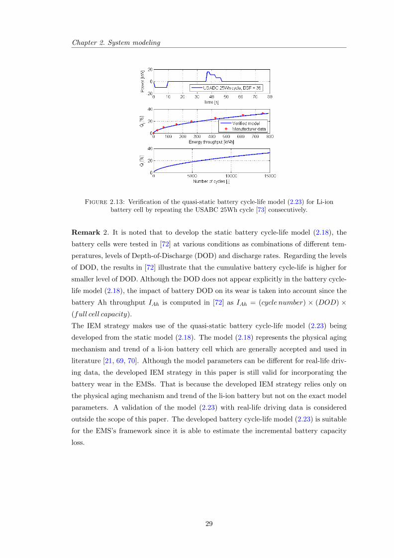
Figure 2.13: Verification of the quasi-static battery cycle-life model (2.23) for Li-ionbattery cell by repeating the USABC 25Wh cycle [73] consecutively.
Remark 2. It is noted that to develop the static battery cycle-life model (2.18), the
battery cells were tested in [72] at various conditions as combinations of different tem-
peratures, levels of Depth-of-Discharge (DOD) and discharge rates. Regarding the levels
of DOD, the results in [72] illustrate that the cumulative battery cycle-life is higher for
smaller level of DOD. Although the DOD does not appear explicitly in the battery cycle-
life model (2.18), the impact of battery DOD on its wear is taken into account since the
battery Ah throughput IAh is computed in [72] as IAh = (cycle number) × (DOD) ×(full cell capacity).
The IEM strategy makes use of the quasi-static battery cycle-life model (2.23) being
developed from the static model (2.18). The model (2.18) represents the physical aging
mechanism and trend of a li-ion battery cell which are generally accepted and used in
literature [21, 69, 70]. Although the model parameters can be different for real-life driv-
ing data, the developed IEM strategy in this paper is still valid for incorporating the
battery wear in the EMSs. That is because the developed IEM strategy relies only on
the physical aging mechanism and trend of the li-ion battery but not on the exact model
parameters. A validation of the model (2.23) with real-life driving data is considered
outside the scope of this paper. The developed battery cycle-life model (2.23) is suitable
for the EMS’s framework since it is able to estimate the incremental battery capacity
loss.
29
2.5. Conclusions
2.5 Conclusions
This chapter presents the quasi-static vehicle model and the component models being
necessary for developing the EMSs and IEMs in chapter 3 and 4. A quasi-static battery
cycle-life model is developed from an empirically model and verified with the battery
manufacturer data. The quasi-static battery cycle-life model is able to estimate the
battery capacity loss every time instant when the battery is charged/discharged. It,
henceforth, provides a basis for integrating the battery wear management in the energy
management of the hybrid truck.
In Chapter 5, simulations will be done to evaluate the developed EMS and IEM strategies
performance. In the simulation environment, the approximated models for the ICE (2.3),
for the MG (2.5) and for the battery efficiency (2.15) are not used. The ICE model is
implemented using a static look-up table expressing the measured fuel consumption for
each operating point of the ICE, defined by the ICE angular speed ω and the ICE power
PICE . Similarly, a static look-up table is utilized to describe the speed dependence
relation between the measured mechanical and electric power of the MG. The battery
efficiency model is obtained from the battery manufacturer.
30
Chapter 3
Analytical solutions for energy
management
To provide fundamental understanding for both mathematical and physical insight of
the energy management in the considered hybrid truck, this chapter presents the ana-
lytical solutions to the predefined fuel minimization Optimal Control Problems (OCPs)
in Table 1.2. The solutions are based on the Equivalent fuel Consumption Minimiza-
tion Strategy (ECMS) technique to determine the optimal hybrid truck operating mode
(Power Supply Mode (PSM), Motor Only (MO), ICE Only, Motor Assist (MA), Charg-
ing (C) and Regenerative Braking (R)) regarding the fuel reduction performance and/or
battery life preservation. A Hamiltonian function is formulated in the ECMS to handle
the balance between the fuel cost and other related costs in the system. The optimal
battery charge/discharge power at its terminal and the operation of the clutch system
are found to minimize the Hamiltonian function.
Regarding the Conventional Energy Management (CEM) CEM1 and CEM2 problem
where the battery life requirement is not taken into account, the Hamiltonian function
is constructed to balance only the fuel and the electric power cost. Minimization of
the Hamiltonian function is shown explicitly to provide the fundamental of the Energy
Management Strategy (EMS) in fuel saving in the hybrid truck. Moreover, the fuel re-
duction improvement from using the Motor Generator (MG) clutch in the clutch system
is also explained by analyzing the derived analytical solution of CEM1.
When the battery life requirement is considered in the Integrated Energy Management
(IEM) IEM1 and IEM2, compared to the conventional ECMS approach [37], the Hamil-
tonian function is extended to incorporate the battery capacity loss state. The aug-
mented Hamiltonian function balances the costs among the fuel consumption, electric
power from (dis-) charging the battery and the battery capacity loss (representing the
battery wear). The analytical solutions to IEM1 and IEM2 are also derived to reveal
31
3.1. Analytical solution for energy management without battery life requirement
the physical insight into the battery life preservation within the EMS framework.
We assume in this chapter that the battery temperature is kept constant by means of
the active Battery Thermal Management System (BTMS) and the future information of
the driving cycle are known. These assumptions are needed to find the optimal control
parameters of the derived solutions of CEM1, CEM2, IEM1 and IEM2.
Analytical solutions for CEM1 and CEM2 are presented in 3.1 and 3.2, respectively.
Analytical solutions for IEM1 and IEM2 are given correspondingly in 3.3 and 3.4. Sec-
tion 3.5 demonstrates the integration of battery temperature dynamics and the BTMS’s
operation in the IEM framework.
3.1 Analytical solution for energy management without
battery life requirement
The objective of CEM1 is to minimize the fuel consumption while taking into account
the battery charge sustaining condition. Using Pontryagin’s Minimum Principle [47],
the Hamiltonian function is formulated from the objective function J =tf∫t0
mf (τ) dτ and
the battery energy state dynamic Es as
H = mf + pEs (3.1)
where p is a multiplier, also known as co-state. Physically, the Hamiltonian function
(3.1) balances the costs between the fuel consumption and electric power from (dis-)
charging the battery. Since p is normally negatively valued, we denote λ1 = −p for the
sake of deriving an explicit solution to CEM1. The Hamiltonian function becomes
H = mf − λ1Es (3.2)
= mf − λ1
(Pb − βP 2
b
)(3.3)
where the ICE fuel mass flow mf can be written as a function of the control inputs and
measured signals Pd and Pl,
mf = α1
(Pd + max
(η−e (Pb + Pl),
Pb + Pl
η+e
)+ g0SMG
)+ α2SICE (3.4)
Due to the discrete values of SICE and SMG as well as of the MG model, (3.4) implies
that the Hamiltonian function H is non differentiable with respect to the control inputs
SICE , SMG and Pb. Nevertheless, H is differentiable with respect to Es. The Maximum
Principle as in Theorem 9.3.1 in [74] is applied to derive the necessary conditions for the
optimal solution of CEM1
32
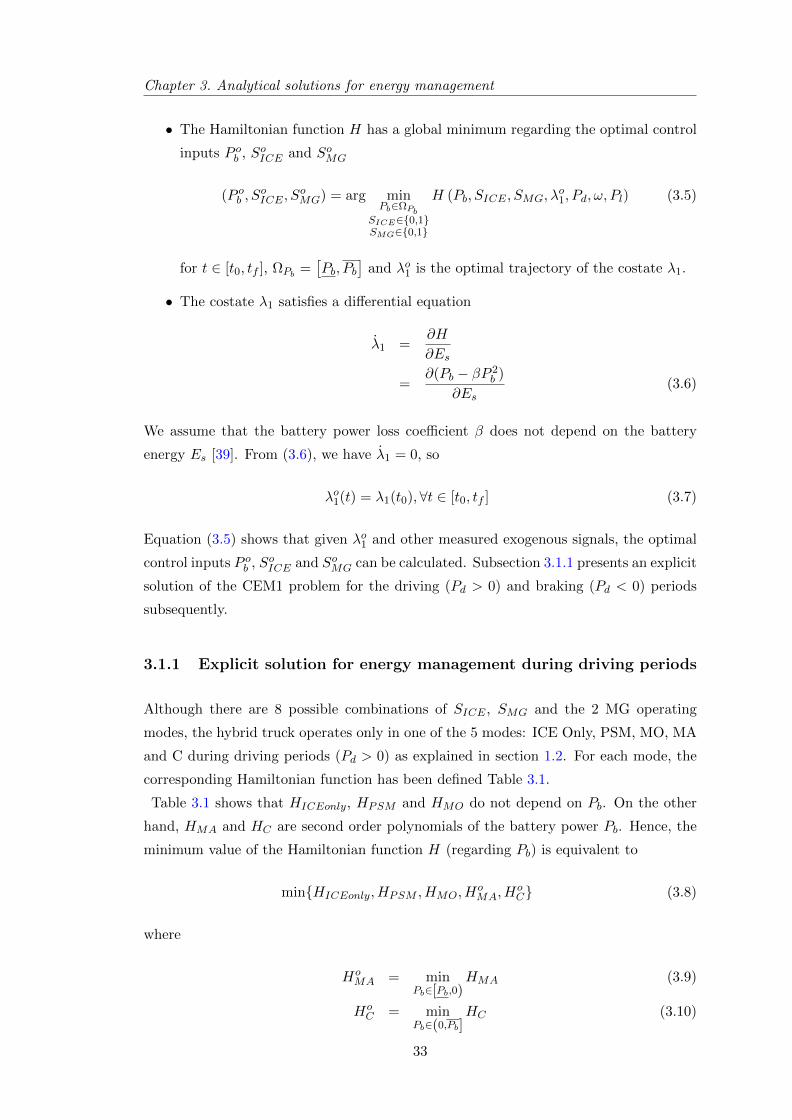
Chapter 3. Analytical solutions for energy management
• The Hamiltonian function H has a global minimum regarding the optimal control
inputs P ob , SoICE and SoMG
(P ob , SoICE , S
oMG) = arg min
Pb∈ΩPbSICE∈0,1SMG∈0,1
H (Pb, SICE , SMG, λo1, Pd, ω, Pl) (3.5)
for t ∈ [t0, tf ], ΩPb =[Pb, Pb
]and λo1 is the optimal trajectory of the costate λ1.
• The costate λ1 satisfies a differential equation
λ1 =∂H
∂Es
=∂(Pb − βP 2
b )
∂Es(3.6)
We assume that the battery power loss coefficient β does not depend on the battery
energy Es [39]. From (3.6), we have λ1 = 0, so
λo1(t) = λ1(t0),∀t ∈ [t0, tf ] (3.7)
Equation (3.5) shows that given λo1 and other measured exogenous signals, the optimal
control inputs P ob , SoICE and SoMG can be calculated. Subsection 3.1.1 presents an explicit
solution of the CEM1 problem for the driving (Pd > 0) and braking (Pd < 0) periods
subsequently.
3.1.1 Explicit solution for energy management during driving periods
Although there are 8 possible combinations of SICE , SMG and the 2 MG operating
modes, the hybrid truck operates only in one of the 5 modes: ICE Only, PSM, MO, MA
and C during driving periods (Pd > 0) as explained in section 1.2. For each mode, the
corresponding Hamiltonian function has been defined Table 3.1.
Table 3.1 shows that HICEonly, HPSM and HMO do not depend on Pb. On the other
hand, HMA and HC are second order polynomials of the battery power Pb. Hence, the
minimum value of the Hamiltonian function H (regarding Pb) is equivalent to
minHICEonly, HPSM , HMO, HoMA, H
oC (3.8)
where
HoMA = min
Pb∈[Pb,0)HMA (3.9)
HoC = min
Pb∈(0,Pb]HC (3.10)
33
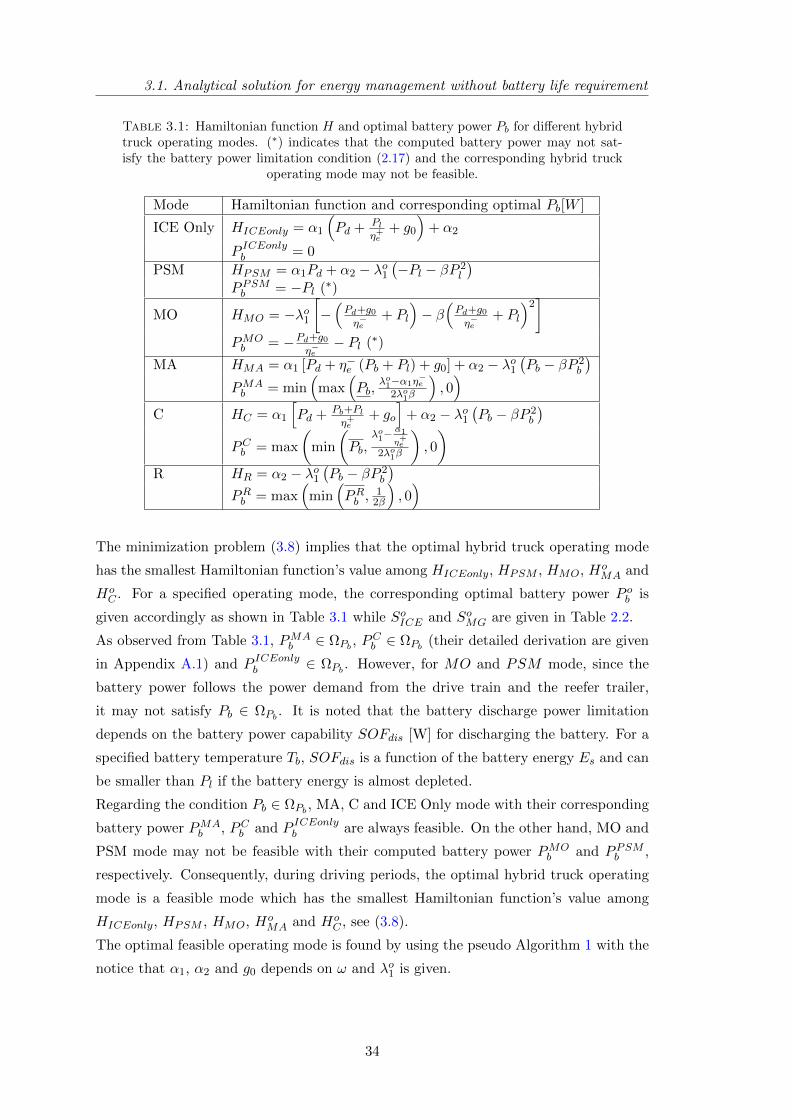
3.1. Analytical solution for energy management without battery life requirement
Table 3.1: Hamiltonian function H and optimal battery power Pb for different hybridtruck operating modes. (∗) indicates that the computed battery power may not sat-isfy the battery power limitation condition (2.17) and the corresponding hybrid truck
operating mode may not be feasible.
Mode Hamiltonian function and corresponding optimal Pb[W ]
ICE Only HICEonly = α1
(Pd + Pl
η+e+ g0
)+ α2
P ICEonlyb = 0
PSM HPSM = α1Pd + α2 − λo1(−Pl − βP 2
l
)PPSMb = −Pl (∗)
MO HMO = −λo1[−(Pd+g0η−e
+ Pl
)− β
(Pd+g0η−e
+ Pl
)2]
PMOb = −Pd+g0
η−e− Pl (∗)
MA HMA = α1 [Pd + η−e (Pb + Pl) + g0] + α2 − λo1(Pb − βP 2
b
)PMAb = min
(max
(Pb,
λo1−α1η−e
2λo1β
), 0)
C HC = α1
[Pd + Pb+Pl
η+e+ go
]+ α2 − λo1
(Pb − βP 2
b
)PCb = max
(min
(Pb,
λo1−α1
η+e2λo1β
), 0
)R HR = α2 − λo1
(Pb − βP 2
b
)PRb = max
(min
(PRb ,
12β
), 0)
The minimization problem (3.8) implies that the optimal hybrid truck operating mode
has the smallest Hamiltonian function’s value among HICEonly, HPSM , HMO, HoMA and
HoC . For a specified operating mode, the corresponding optimal battery power P ob is
given accordingly as shown in Table 3.1 while SoICE and SoMG are given in Table 2.2.
As observed from Table 3.1, PMAb ∈ ΩPb , P
Cb ∈ ΩPb (their detailed derivation are given
in Appendix A.1) and P ICEonlyb ∈ ΩPb . However, for MO and PSM mode, since the
battery power follows the power demand from the drive train and the reefer trailer,
it may not satisfy Pb ∈ ΩPb . It is noted that the battery discharge power limitation
depends on the battery power capability SOFdis [W] for discharging the battery. For a
specified battery temperature Tb, SOFdis is a function of the battery energy Es and can
be smaller than Pl if the battery energy is almost depleted.
Regarding the condition Pb ∈ ΩPb , MA, C and ICE Only mode with their corresponding
battery power PMAb , PCb and P ICEonlyb are always feasible. On the other hand, MO and
PSM mode may not be feasible with their computed battery power PMOb and PPSMb ,
respectively. Consequently, during driving periods, the optimal hybrid truck operating
mode is a feasible mode which has the smallest Hamiltonian function’s value among
HICEonly, HPSM , HMO, HoMA and Ho
C , see (3.8).
The optimal feasible operating mode is found by using the pseudo Algorithm 1 with the
notice that α1, α2 and g0 depends on ω and λo1 is given.
34
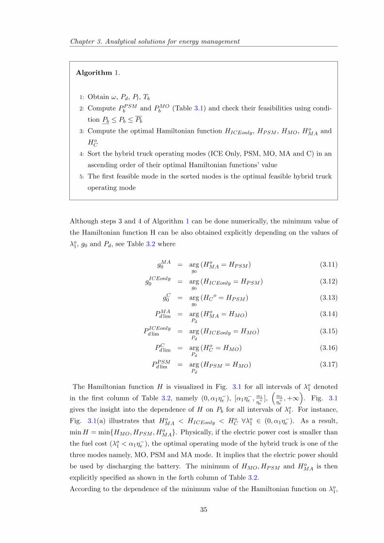
Chapter 3. Analytical solutions for energy management
Algorithm 1.
1: Obtain ω, Pd, Pl, Tb
2: Compute PPSMb and PMOb (Table 3.1) and check their feasibilities using condi-
tion Pb ≤ Pb ≤ Pb3: Compute the optimal Hamiltonian function HICEonly, HPSM , HMO, Ho
MA and
HoC
4: Sort the hybrid truck operating modes (ICE Only, PSM, MO, MA and C) in an
ascending order of their optimal Hamiltonian functions’ value
5: The first feasible mode in the sorted modes is the optimal feasible hybrid truck
operating mode
Although steps 3 and 4 of Algorithm 1 can be done numerically, the minimum value of
the Hamiltonian function H can be also obtained explicitly depending on the values of
λo1, g0 and Pd, see Table 3.2 where
gMA0 = arg
g0(Ho
MA = HPSM ) (3.11)
gICEonly0 = argg0
(HICEonly = HPSM ) (3.12)
gC0 = argg0
(HCo = HPSM ) (3.13)
PMAd lim = arg
Pd
(HoMA = HMO) (3.14)
P ICEonlyd lim = argPd
(HICEonly = HMO) (3.15)
PCd lim = argPd
(HoC = HMO) (3.16)
PPSMd lim = argPd
(HPSM = HMO) (3.17)
The Hamiltonian function H is visualized in Fig. 3.1 for all intervals of λo1 denoted
in the first column of Table 3.2, namely (0, α1η−e ), [α1η
−e ,
α1
η+e],(α1
η+e,+∞
). Fig. 3.1
gives the insight into the dependence of H on Pb for all intervals of λo1. For instance,
Fig. 3.1(a) illustrates that HoMA < HICEonly < Ho
C ∀λo1 ∈ (0, α1η−e ). As a result,
minH = minHMO, HPSM , HoMA. Physically, if the electric power cost is smaller than
the fuel cost (λo1 < α1η−e ), the optimal operating mode of the hybrid truck is one of the
three modes namely, MO, PSM and MA mode. It implies that the electric power should
be used by discharging the battery. The minimum of HMO, HPSM and HoMA is then
explicitly specified as shown in the forth column of Table 3.2.
According to the dependence of the minimum value of the Hamiltonian function on λo1,
35
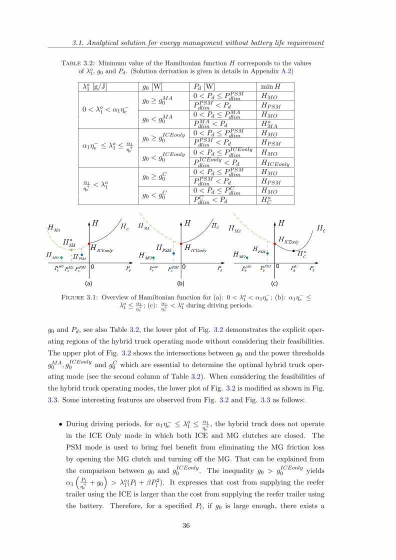
3.1. Analytical solution for energy management without battery life requirement
Table 3.2: Minimum value of the Hamiltonian function H corresponds to the valuesof λo1, g0 and Pd. (Solution derivation is given in details in Appendix A.2)
λo1 [g/J] g0 [W] Pd [W] minH
0 < λo1 < α1η−e
g0 ≥ gMA0
0 < Pd ≤ PPSMdlim HMO
PPSMdlim < Pd HPSM
g0 < gMA0
0 < Pd ≤ PMAdlim HMO
PMAdlim < Pd Ho
MA
α1η−e ≤ λo1 ≤ α1
η+e
g0 ≥ gICEonly0
0 < Pd ≤ PPSMdlim HMO
PPSMdlim < Pd HPSM
g0 < gICEonly0
0 < Pd ≤ P ICEonlydlim HMO
P ICEonlydlim < Pd HICEonly
α1
η+e< λo1
g0 ≥ gC00 < Pd ≤ PPSMdlim HMO
PPSMdlim < Pd HPSM
g0 < gC00 < Pd ≤ PCdlim HMO
PCdlim < Pd HoC
Figure 3.1: Overview of Hamiltonian function for (a): 0 < λo1 < α1η−e ; (b): α1η
−e ≤
λo1 ≤ α1
η+e; (c): α1
η+e< λo1 during driving periods.
g0 and Pd, see also Table 3.2, the lower plot of Fig. 3.2 demonstrates the explicit oper-
ating regions of the hybrid truck operating mode without considering their feasibilities.
The upper plot of Fig. 3.2 shows the intersections between g0 and the power thresholds
gMA0 , gICEonly0 and gC0 which are essential to determine the optimal hybrid truck oper-
ating mode (see the second column of Table 3.2). When considering the feasibilities of
the hybrid truck operating modes, the lower plot of Fig. 3.2 is modified as shown in Fig.
3.3. Some interesting features are observed from Fig. 3.2 and Fig. 3.3 as follows:
• During driving periods, for α1η−e ≤ λo1 ≤ α1
η+e, the hybrid truck does not operate
in the ICE Only mode in which both ICE and MG clutches are closed. The
PSM mode is used to bring fuel benefit from eliminating the MG friction loss
by opening the MG clutch and turning off the MG. That can be explained from
the comparison between g0 and gICEonly0 . The inequality g0 > gICEonly0 yields
α1
(Plη+e
+ g0
)> λo1(Pl + βP 2
l ). It expresses that cost from supplying the reefer
trailer using the ICE is larger than the cost from supplying the reefer trailer using
the battery. Therefore, for a specified Pl, if g0 is large enough, there exists a
36
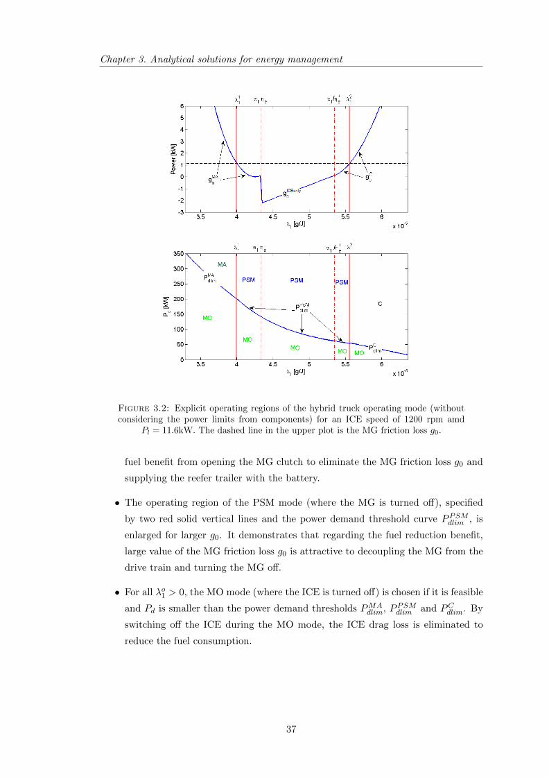
Chapter 3. Analytical solutions for energy management
Figure 3.2: Explicit operating regions of the hybrid truck operating mode (withoutconsidering the power limits from components) for an ICE speed of 1200 rpm amd
Pl = 11.6kW. The dashed line in the upper plot is the MG friction loss g0.
fuel benefit from opening the MG clutch to eliminate the MG friction loss g0 and
supplying the reefer trailer with the battery.
• The operating region of the PSM mode (where the MG is turned off), specified
by two red solid vertical lines and the power demand threshold curve PPSMdlim , is
enlarged for larger g0. It demonstrates that regarding the fuel reduction benefit,
large value of the MG friction loss g0 is attractive to decoupling the MG from the
drive train and turning the MG off.
• For all λo1 > 0, the MO mode (where the ICE is turned off) is chosen if it is feasible
and Pd is smaller than the power demand thresholds PMAdlim, PPSMdlim and PCdlim. By
switching off the ICE during the MO mode, the ICE drag loss is eliminated to
reduce the fuel consumption.
37
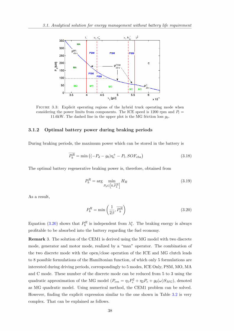
3.1. Analytical solution for energy management without battery life requirement
Figure 3.3: Explicit operating regions of the hybrid truck operating mode whenconsidering the power limits from components. The ICE speed is 1200 rpm and Pl =
11.6kW. The dashed line in the upper plot is the MG friction loss g0.
3.1.2 Optimal battery power during braking periods
During braking periods, the maximum power which can be stored in the battery is
PRb = min((−Pd − g0)η+
e − Pl, SOFcha)
(3.18)
The optimal battery regenerative braking power is, therefore, obtained from
PRb = arg minPb∈
(0,PRb
]HR (3.19)
As a result,
PRb = min
(1
2β, PRb
)(3.20)
Equation (3.20) shows that PRb is independent from λo1. The braking energy is always
profitable to be absorbed into the battery regarding the fuel economy.
Remark 3. The solution of the CEM1 is derived using the MG model with two discrete
mode, generator and motor mode, realized by a “max” operator. The combination of
the two discrete mode with the open/close operation of the ICE and MG clutch leads
to 8 possible formulations of the Hamiltonian function, of which only 5 formulations are
interested during driving periods, correspondingly to 5 modes, ICE Only, PSM, MO, MA
and C mode. These number of the discrete mode can be reduced from 5 to 3 using the
quadratic approximation of the MG model (Pem = η1P2e + η2Pe + g0(ω)SMG), denoted
as MG quadratic model. Using numerical method, the CEM1 problem can be solved.
However, finding the explicit expression similar to the one shown in Table 3.2 is very
complex. That can be explained as follows.
38
Chapter 3. Analytical solutions for energy management
Using the MG quadratic model, the Hamiltonian functions for the MA, ICE Only and
C mode are now generalized as
HMIC = α1
(Pd + η1(Pb + Pl)
2 + η2 (Pb + Pl) + g0(ω)SMG
)+ α2SICE
−λo1(Pb − βP 2
b
)(3.21)
The minimum value of the Hamiltonian function H is now equivalent to
H = minHoMIC , HPSM , HMO (3.22)
where
HoMIC = min
Pb∈[Pb,Pb]HMIC (3.23)
Moreover, it is noteworthy that using the MG quadratic model, the battery power during
the MO mode is obtained as
PMOb = arg
Pb
(η1(Pb + Pl)
2 + η2 (Pb + Pl) + g0 = −Pd)
(3.24)
as a result,
PMOb =
−η2 ±√η2
2 − 4 (Pd + g0) η1
2η1− Pl (3.25)
The existence of the square root in PMOb leads to an existence of the square root in
HMO. Consequently, the analytical expressions of the power thresholds
PPSMdlim = argPd
(HPSM = HMO) (3.26)
PMICdlim = arg
Pd
(HoMIC = HMO) (3.27)
are very complex to be derived.
3.2 Solution for energy management with battery energy
state constraint and without battery life requirement
The obtained solution for CEM1 does not take into account the battery energy state
constraint (Es ≤ Es(t) ≤ Es). Consequently, the battery energy Es may exceed Es or
goes below Es. This section extends the solution of CEM1 to take into account also the
battery energy state constraint.
39
3.3. Analytical solution for integrated energy management
When considering the battery energy state constraint, besides the necessary conditions
(3.5) and (3.6), additional conditions are needed. Specifically, for any (unknown) time
instants tl and tu when Es correspondingly hits Es and Es, the costate λ1 trajectory
may have a discontinuity given by the following jump conditions [75]:
λ1
(t+l)
= λ1
(t−l)− ηl (tl)
∂(Es − Es (tl)
)∂Es (tl)
= λ1
(t−l)
+ ηl (tl) (3.28)
λ1
(t+u)
= λ1
(t−u)− ηu (tu)
∂(Es − Es
)∂Es (tu)
= λ1
(t−u)− ηu (tu) (3.29)
The superscripts − and + represent correspondingly the left-hand and right-hand side
limits values at the contact times. ηl ≥ 0 and ηu ≥ 0 are the magnitude of the jump
of the costate λ1 when the battery energy Es hits its boundaries. From (3.6), (3.28)
and (3.29), the optimal trajectory of the costate λ1 is piecewise constant, where a jump
occurs if the battery energy state boundaries Es and Es are reached (see also [23] for
similar observation). To find λo1, the Recursive root finding Algorithm in [23] is adopted
without modifying the explicit solution denoted in Algorithm 1 and Table 3.2.
3.3 Analytical solution for integrated energy management
The IEM1 strategy aims at guaranteeing the battery lifetime constraint (Ql(tf ) ≤ Ql)
while allowing appropriate hybrid powertrain operations for fuel minimization. The
strategy uses three control variables namely, battery power Pb, ICE clutch SICE and
MG clutch SMG. This section presents firstly the convexification of the developed battery
cycle-life model. The convexified battery cycyle-life model is utilized to formulate and
solve the IEM1 strategy explicitly to minimize the fuel consumption while satisfying the
battery capacity loss and charge sustaining constraints.
3.3.1 Convexification of battery cycle-life model
As shown in the quasi-static battery cycle-life model, the incremental battery capacity
loss Ql = h (Ps, Tb)Qz−1z
l is a nonlinear function of Ps, Tb and Ql. Moreover, h(Ps, Tb)
has an exponential term making it complex to derive an analytical solution for the IEM1
strategy. Thus, for the sake of deriving an analytical solution for the IEM1 strategy, the
function h(Ps, Tb) is approximated as
h (Pb, Tb) = αb (Tb)P2b (3.30)
40
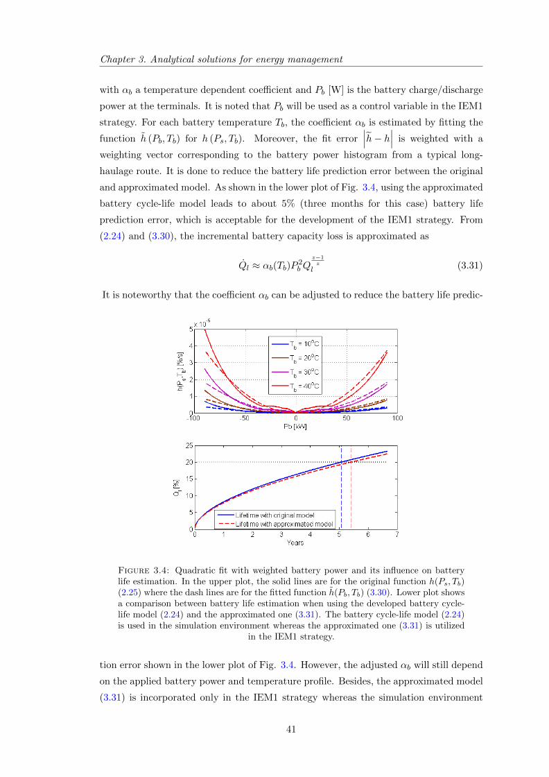
Chapter 3. Analytical solutions for energy management
with αb a temperature dependent coefficient and Pb [W] is the battery charge/discharge
power at the terminals. It is noted that Pb will be used as a control variable in the IEM1
strategy. For each battery temperature Tb, the coefficient αb is estimated by fitting the
function h (Pb, Tb) for h (Ps, Tb). Moreover, the fit error∣∣∣h− h∣∣∣ is weighted with a
weighting vector corresponding to the battery power histogram from a typical long-
haulage route. It is done to reduce the battery life prediction error between the original
and approximated model. As shown in the lower plot of Fig. 3.4, using the approximated
battery cycle-life model leads to about 5% (three months for this case) battery life
prediction error, which is acceptable for the development of the IEM1 strategy. From
(2.24) and (3.30), the incremental battery capacity loss is approximated as
Ql ≈ αb(Tb)P 2b Q
z−1z
l (3.31)
It is noteworthy that the coefficient αb can be adjusted to reduce the battery life predic-
Figure 3.4: Quadratic fit with weighted battery power and its influence on batterylife estimation. In the upper plot, the solid lines are for the original function h(Ps, Tb)(2.25) where the dash lines are for the fitted function h(Pb, Tb) (3.30). Lower plot showsa comparison between battery life estimation when using the developed battery cycle-life model (2.24) and the approximated one (3.31). The battery cycle-life model (2.24)is used in the simulation environment whereas the approximated one (3.31) is utilized
in the IEM1 strategy.
tion error shown in the lower plot of Fig. 3.4. However, the adjusted αb will still depend
on the applied battery power and temperature profile. Besides, the approximated model
(3.31) is incorporated only in the IEM1 strategy whereas the simulation environment
41
3.3. Analytical solution for integrated energy management
uses (2.23) and (2.24) to estimate Ql. As a result, the approximated model (3.31) is
suitable for the development of the IEM1 strategy.
3.3.2 Extended equivalent fuel consumption management strategy ap-
proach
To solve the predefined problem IEM1, an ECMS technique [37], [23] is extended. Com-
pared to the conventional ECMS approach, the Hamiltonian function is extended to take
into account not only the battery energy Es but also the battery capacity loss Ql. The
augmented Hamiltonian function is formulated as
H = mf + pEs + λ2Ql (3.32)
where p [g/J] and λ2 [g/%] are the multipliers, also known as costates. The variable p is
normally negatively valued. Hence, for the sake of simplifying the solution derivation, we
introduce λ1 = −p [g/J]. From Ql = h (Ps, Tb)Qz−1z
l and Es = Pb−βP 2b , the Hamiltonian
function H becomes
H = mf − λ1
(Pb − βP 2
b
)+ λ2h (Ps, Tb)Q
z−1z
l (3.33)
Physically, the Hamiltonian function (3.33) balances the incremental fuel consumption,
battery charge/discharge power (via λ1) and the incremental battery capacity loss (via
λ2) at every time instant when the battery is charged/discharged. The necessary con-
ditions for the optimal costates λ1 and λ2 are derived as [74]
λ1 =∂H
∂Es= −λ1
∂(Pb − βP 2b )
∂Es(3.34)
λ2 = − ∂H∂Ql
(3.35)
Often it is assumed that the battery power loss coefficient β does not depend on the
battery energy Es [15], [39]. Hence, from equation (3.34), we have λ1 = 0. As a result,
λ1(t) = λ1(t0),∀t ∈ [t0, tf ] (3.36)
Moreover, from (3.33) and (3.35), the optimal trajectory of the costate λ2 can be ob-
tained as
λ2 = −λ2h(Ps, Tb)z − 1
zQ− 1z
l (3.37)
↔ dλ2
λ2= −h(Ps, Tb)
z − 1
zQ− 1z
l dt (3.38)
42
Chapter 3. Analytical solutions for energy management
Substitute dt = dQl
h(Ps,Tb)Qz−1z
l
from (2.24) into (3.38), we obtain
dλ2
λ2= −z − 1
z
dQlQl
(3.39)
The explicit expression of the optimal trajectory of the co-state λ2 is derived as
λ2 (t) = λ2 (t0)Q− z−1
zl (t) (3.40)
Equation (3.40) shows that to obtain the optimal trajectory of the co-state λ2, it is
required to search for an optimal initial value λ2(t0) only.
For the sake of simplification, λ1(t0) and λ2(t0) are denoted as λo1 and λo2, respectively.
Substitute λ1(t) and λ2(t) from (3.36) and (3.40) in the Hamiltonian function (3.33), we
have
General formulation :H = mf − λo1(Pb − βP 2
b
)+ λo2h(Ps, Tb) (3.41)
The general formulation of the Hamiltonian function H (3.41) elucidates the necessity
of using the additional co-state λ2 for obtaining the optimal battery power in the IEM1
strategy for a general formulation of the battery cycle-life model (2.24).
In this thesis we use the function (3.31) Ql ≈ αb(Tb)P 2b Q
z−1z
l to approximate the battery
wear and to derive an analytical solution to achieve mathematical and physical insight
regarding the battery life preservation in the EMS framework. The Hamiltonian function
(3.41) is now denoted as
Specific formulation with approximated battery cycle − life model (3 .31 ) :
H = mf − λo1(Pb − βP 2
b
)+ λo2αbP
2b (3.42)
Given λo1 and λo2, the optimal battery power P ob , ICE clutch SoICE and MG clutch SoMG
can be obtained by solving the following minimization problem
minPb∈ΩPb
SICE∈0,1SMG∈0,1
H (Pb, SICE , SMG, λo1, λ
o2, Pd, ω, Pl) (3.43)
where ΩPb =[Pb, Pb
]. The following subsection presents the explicit solution of the
minimization problem (3.43) for the driving (Pd > 0) and braking (Pd ≤ 0) periods
subsequently.
Remark 4. With the particular approximation Ql ≈ αb(Tb)P 2b Q
z−1z
l of the battery cycle-
life model, it shows an equivalence between using λ2 and adapting the battery power
43
3.3. Analytical solution for integrated energy management
loss coefficient β to satisfy the battery capacity loss constraint Ql(tf ) ≤ Ql. The Hamil-
tonian function (3.42) can be denoted as H = mf−λo1(Pb − β
′P 2b
)where β
′= β+
λo2αbλo1
.
Generally, to satisfy the constraints on battery energy and capacity loss states, using λ1
and β′
is a subclass of using λ1 and λ2.
Using λ1 and β′
to guarantee the battery energy and capacity loss constraints, the
explicit solution of the CEM1 strategy can be used without any modification except
replacing β by β′. The battery power loss coefficient β in the CEM1 strategy is a phys-
ical parameter of the battery efficiency model whereas the adapted battery power loss
coefficient β′
is used as a control variable to assure the battery capacity loss constraint.
Using only one co-state λ1 is sufficient to obtain the optimal solution of the CEM1 strat-
egy since the battery capacity loss constraint is not considered in the CEM1 strategy.
When the battery capacity loss constraint is taken into account, we need two indepen-
dent co-states λ1, λ2 or two control variables (a co-state λ1 and a control variable β′)
to satisfy the constraints on the battery energy and capacity loss state.
3.3.3 Explicit solution for integrated energy management during driv-
ing periods
Owing to the MG model (Pem = max(η−e Pe,
Peη+e
)+ g0 (ω)SMG) and the discrete control
variables SICE and SMG, the Hamiltonian function H in (3.43) is not smooth. Specif-
ically, the Hamiltonian function H switches accordingly to different combinations of
SICE , SMG and the MG operating modes (generator or motor mode). Although there
are 8 possible combinations of SICE , SMG and the 2 MG operating modes, the hybrid
truck operates only in one of the 5 modes: ICE Only, PSM, MO, MA and C during driv-
ing periods, as explained in section 1.2. For each mode, the corresponding Hamiltonian
function has been defined Table 3.3. Table 3.3 shows that HICEonly, HPSM and HMO
do not depend on Pb. On the other hand, HMA and HC are second order polynomials
of the battery power Pb. Hence, the minimum value of the Hamiltonian function H
(regarding Pb) is equivalent to
minHICEonly, HPSM , HMO, HoMA, H
oC (3.44)
where
HoMA = min
Pb∈[Pb,0)HMA (3.45)
HoC = min
Pb∈(0,Pb]HC (3.46)
44
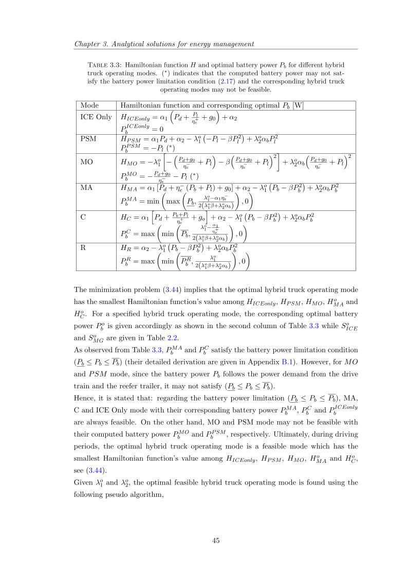
Chapter 3. Analytical solutions for energy management
Table 3.3: Hamiltonian function H and optimal battery power Pb for different hybridtruck operating modes. (∗) indicates that the computed battery power may not sat-isfy the battery power limitation condition (2.17) and the corresponding hybrid truck
operating modes may not be feasible.
Mode Hamiltonian function and corresponding optimal Pb [W]
ICE Only HICEonly = α1
(Pd + Pl
η+e+ g0
)+ α2
P ICEonlyb = 0
PSM HPSM = α1Pd + α2 − λo1(−Pl − βP 2
l
)+ λo2αbP
2l
PPSMb = −Pl (∗)
MO HMO = −λo1[−(Pd+g0η−e
+ Pl
)− β
(Pd+g0η−e
+ Pl
)2]
+ λo2αb
(Pd+g0η−e
+ Pl
)2
PMOb = −Pd+g0
η−e− Pl (∗)
MA HMA = α1 [Pd + η−e (Pb + Pl) + g0] + α2 − λo1(Pb − βP 2
b
)+ λo2αbP
2b
PMAb = min
(max
(Pb,
λo1−α1η−e
2(λo1β+λo2αb)
), 0
)C HC = α1
[Pd + Pb+Pl
η+e+ go
]+ α2 − λo1
(Pb − βP 2
b
)+ λo2αbP
2b
PCb = max
(min
(Pb,
λo1−α1
η+e
2(λo1β+λo2αb)
), 0
)R HR = α2 − λo1
(Pb − βP 2
b
)+ λo2αbP
2b
PRb = max
(min
(PRb ,
λo12(λo1β+λo2αb)
), 0
)
The minimization problem (3.44) implies that the optimal hybrid truck operating mode
has the smallest Hamiltonian function’s value among HICEonly, HPSM , HMO, HoMA and
HoC . For a specified hybrid truck operating mode, the corresponding optimal battery
power P ob is given accordingly as shown in the second column of Table 3.3 while SoICE
and SoMG are given in Table 2.2.
As observed from Table 3.3, PMAb and PCb satisfy the battery power limitation condition
(Pb ≤ Pb ≤ Pb) (their detailed derivation are given in Appendix B.1). However, for MO
and PSM mode, since the battery power Pb follows the power demand from the drive
train and the reefer trailer, it may not satisfy (Pb ≤ Pb ≤ Pb).Hence, it is stated that: regarding the battery power limitation (Pb ≤ Pb ≤ Pb), MA,
C and ICE Only mode with their corresponding battery power PMAb , PCb and P ICEonlyb
are always feasible. On the other hand, MO and PSM mode may not be feasible with
their computed battery power PMOb and PPSMb , respectively. Ultimately, during driving
periods, the optimal hybrid truck operating mode is a feasible mode which has the
smallest Hamiltonian function’s value among HICEonly, HPSM , HMO, HoMA and Ho
C ,
see (3.44).
Given λo1 and λo2, the optimal feasible hybrid truck operating mode is found using the
following pseudo algorithm,
45
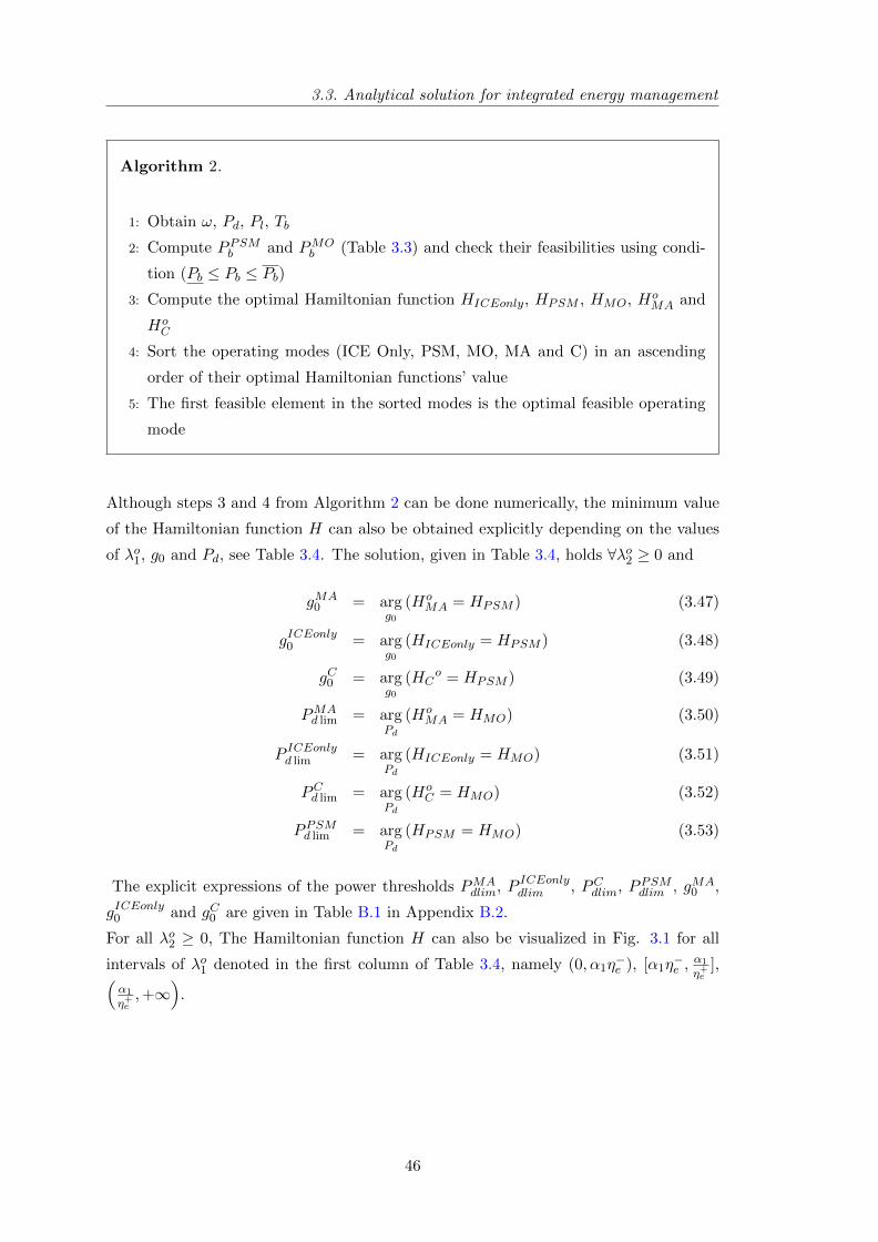
3.3. Analytical solution for integrated energy management
Algorithm 2.
1: Obtain ω, Pd, Pl, Tb
2: Compute PPSMb and PMOb (Table 3.3) and check their feasibilities using condi-
tion (Pb ≤ Pb ≤ Pb)3: Compute the optimal Hamiltonian function HICEonly, HPSM , HMO, Ho
MA and
HoC
4: Sort the operating modes (ICE Only, PSM, MO, MA and C) in an ascending
order of their optimal Hamiltonian functions’ value
5: The first feasible element in the sorted modes is the optimal feasible operating
mode
Although steps 3 and 4 from Algorithm 2 can be done numerically, the minimum value
of the Hamiltonian function H can also be obtained explicitly depending on the values
of λo1, g0 and Pd, see Table 3.4. The solution, given in Table 3.4, holds ∀λo2 ≥ 0 and
gMA0 = arg
g0(Ho
MA = HPSM ) (3.47)
gICEonly0 = argg0
(HICEonly = HPSM ) (3.48)
gC0 = argg0
(HCo = HPSM ) (3.49)
PMAd lim = arg
Pd
(HoMA = HMO) (3.50)
P ICEonlyd lim = argPd
(HICEonly = HMO) (3.51)
PCd lim = argPd
(HoC = HMO) (3.52)
PPSMd lim = argPd
(HPSM = HMO) (3.53)
The explicit expressions of the power thresholds PMAdlim, P ICEonlydlim , PCdlim, PPSMdlim , gMA
0 ,
gICEonly0 and gC0 are given in Table B.1 in Appendix B.2.
For all λo2 ≥ 0, The Hamiltonian function H can also be visualized in Fig. 3.1 for all
intervals of λo1 denoted in the first column of Table 3.4, namely (0, α1η−e ), [α1η
−e ,
α1
η+e],(
α1
η+e,+∞
).
46
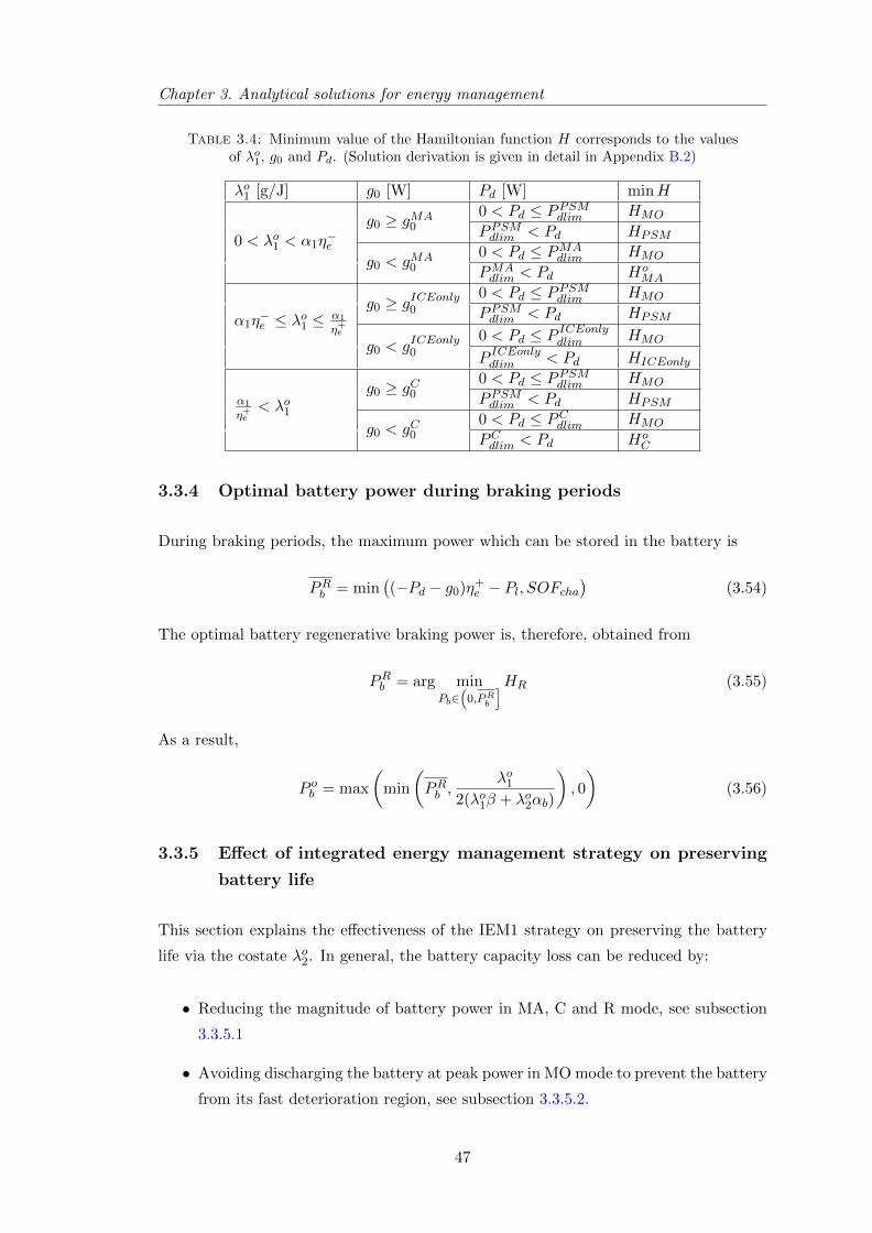
Chapter 3. Analytical solutions for energy management
Table 3.4: Minimum value of the Hamiltonian function H corresponds to the valuesof λo1, g0 and Pd. (Solution derivation is given in detail in Appendix B.2)
λo1 [g/J] g0 [W] Pd [W] minH
0 < λo1 < α1η−e
g0 ≥ gMA0
0 < Pd ≤ PPSMdlim HMO
PPSMdlim < Pd HPSM
g0 < gMA0
0 < Pd ≤ PMAdlim HMO
PMAdlim < Pd Ho
MA
α1η−e ≤ λo1 ≤ α1
η+e
g0 ≥ gICEonly0
0 < Pd ≤ PPSMdlim HMO
PPSMdlim < Pd HPSM
g0 < gICEonly0
0 < Pd ≤ P ICEonlydlim HMO
P ICEonlydlim < Pd HICEonly
α1
η+e< λo1
g0 ≥ gC00 < Pd ≤ PPSMdlim HMO
PPSMdlim < Pd HPSM
g0 < gC00 < Pd ≤ PCdlim HMO
PCdlim < Pd HoC
3.3.4 Optimal battery power during braking periods
During braking periods, the maximum power which can be stored in the battery is
PRb = min((−Pd − g0)η+
e − Pl, SOFcha)
(3.54)
The optimal battery regenerative braking power is, therefore, obtained from
PRb = arg minPb∈
(0,PRb
]HR (3.55)
As a result,
P ob = max
(min
(PRb ,
λo12(λo1β + λo2αb)
), 0
)(3.56)
3.3.5 Effect of integrated energy management strategy on preserving
battery life
This section explains the effectiveness of the IEM1 strategy on preserving the battery
life via the costate λo2. In general, the battery capacity loss can be reduced by:
• Reducing the magnitude of battery power in MA, C and R mode, see subsection
3.3.5.1
• Avoiding discharging the battery at peak power in MO mode to prevent the battery
from its fast deterioration region, see subsection 3.3.5.2.
47
3.3. Analytical solution for integrated energy management
• Reducing the number of occurrences of PSM mode and favoring the usage of ICE
Only mode, see subsection 3.3.5.3
3.3.5.1 Influence of IEM1 strategy on battery usage in MA, C and R mode
As defined in the third column of Table 3.1, the costate λo2 appears only in the denomi-
nator of the equations of the battery power PMAb , PCb and PRb . Since λo1, α1, αb, β and
λo2 are positive, the sign of battery power during MA, C and R mode is not influenced by
λo2. Hence, the costate λo2 only affects the magnitude of PMAb , PCb and PRb . Specifically,
an increase of λo2 reduces the magnitude of PMAb , PCb and PRb .
It is interesting to note that in the equations of PMAb and PCb , the numerators show the
comparison between the cost of electric power and fuel, represented by λo1 and α1. As
described in Table 2.2, the battery power is negative in MA mode. As a result, MA
mode is only selected for λo1 < α1η−e . Physically, it means that the MA mode can only
be selected when the electric power from the battery is cheaper than electric power from
fuel. In contrast, the C mode is only selected when the fuel cost is cheaper than the
electric power cost, λo1 >αo1η+e
.
The denominators in the equations of PMAb , PCb and PRb on the other hand, are the total
cost of the battery power loss and the capacity loss during its operation. It suggests
that the costate λo2 tries to add an additional penalty to the cost of the battery power
loss to restrict the battery usage. This observation aligns with an approach proposed
in [63] and chapter 4 where an adaptive factor is introduced to artificially increase the
battery power loss when reducing the battery wear is necessary.
3.3.5.2 Influence of IEM1 strategy on battery usage in MO mode
As shown in Table 3.2, the minimum value of the Hamiltonian function H is HMO if
the driver power demand Pd is smaller than certain power thresholds PMAdlim, P ICEonlydlim ,
PCdlim and PPSMdlim , generalized as Pmodedlim to simplify the notation. The symbol “mode”
represents MA, ICE Only, C and PSM. The MO mode is only selected if Pd ≤ Pmodedlim
and the MO mode is feasible according to the power limitation Pb ≤ Pb ≤ Pb. The
battery power in MO follows the power demand from the drive train Pd and the reefer
trailer Pl. As a result, to restrict the battery power in MO mode, the power demand
limitation curve Pmodedlim should be reduced.
For λo2 > 0, the first derivative of Pmodedlim regarding λo2 satisfies∂Pmoded lim∂λo2
< 0 for all mode ∈ MA, ICE Only, C, PSM . It means that an increase of λo2 leads to a decrease of the
power demand limitation curve Pmodedlim .
To illustrate the above statement, the explicit solution of IEM1 strategy (see Table 3.2)
48
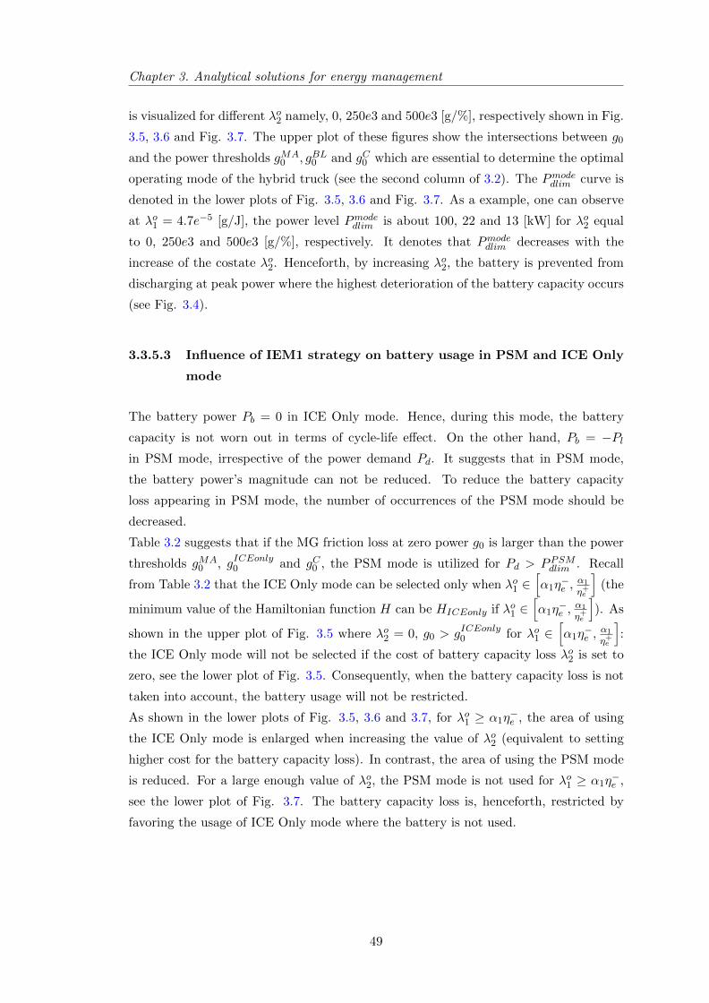
Chapter 3. Analytical solutions for energy management
is visualized for different λo2 namely, 0, 250e3 and 500e3 [g/%], respectively shown in Fig.
3.5, 3.6 and Fig. 3.7. The upper plot of these figures show the intersections between g0
and the power thresholds gMA0 , gBL0 and gC0 which are essential to determine the optimal
operating mode of the hybrid truck (see the second column of 3.2). The Pmodedlim curve is
denoted in the lower plots of Fig. 3.5, 3.6 and Fig. 3.7. As a example, one can observe
at λo1 = 4.7e−5 [g/J], the power level Pmodedlim is about 100, 22 and 13 [kW] for λo2 equal
to 0, 250e3 and 500e3 [g/%], respectively. It denotes that Pmodedlim decreases with the
increase of the costate λo2. Henceforth, by increasing λo2, the battery is prevented from
discharging at peak power where the highest deterioration of the battery capacity occurs
(see Fig. 3.4).
3.3.5.3 Influence of IEM1 strategy on battery usage in PSM and ICE Only
mode
The battery power Pb = 0 in ICE Only mode. Hence, during this mode, the battery
capacity is not worn out in terms of cycle-life effect. On the other hand, Pb = −Plin PSM mode, irrespective of the power demand Pd. It suggests that in PSM mode,
the battery power’s magnitude can not be reduced. To reduce the battery capacity
loss appearing in PSM mode, the number of occurrences of the PSM mode should be
decreased.
Table 3.2 suggests that if the MG friction loss at zero power g0 is larger than the power
thresholds gMA0 , gICEonly0 and gC0 , the PSM mode is utilized for Pd > PPSMdlim . Recall
from Table 3.2 that the ICE Only mode can be selected only when λo1 ∈[α1η
−e ,
α1
η+e
](the
minimum value of the Hamiltonian function H can be HICEonly if λo1 ∈[α1η
−e ,
α1
η+e
]). As
shown in the upper plot of Fig. 3.5 where λo2 = 0, g0 > gICEonly0 for λo1 ∈[α1η
−e ,
α1
η+e
]:
the ICE Only mode will not be selected if the cost of battery capacity loss λo2 is set to
zero, see the lower plot of Fig. 3.5. Consequently, when the battery capacity loss is not
taken into account, the battery usage will not be restricted.
As shown in the lower plots of Fig. 3.5, 3.6 and 3.7, for λo1 ≥ α1η−e , the area of using
the ICE Only mode is enlarged when increasing the value of λo2 (equivalent to setting
higher cost for the battery capacity loss). In contrast, the area of using the PSM mode
is reduced. For a large enough value of λo2, the PSM mode is not used for λo1 ≥ α1η−e ,
see the lower plot of Fig. 3.7. The battery capacity loss is, henceforth, restricted by
favoring the usage of ICE Only mode where the battery is not used.
49
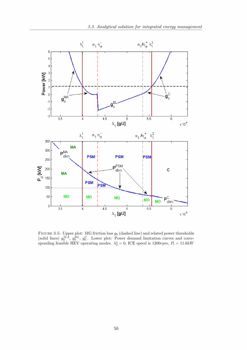
3.3. Analytical solution for integrated energy management
Figure 3.5: Upper plot: MG friction loss g0 (dashed line) and related power thresholds(solid lines) gMA
0 , gBL0 , gC0 . Lower plot: Power demand limitation curves and corre-sponding feasible HEV operating modes. λo2 = 0, ICE speed is 1200rpm, Pl = 11.6kW
50
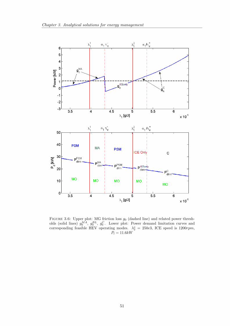
Chapter 3. Analytical solutions for energy management
Figure 3.6: Upper plot: MG friction loss g0 (dashed line) and related power thresh-olds (solid lines) gMA
0 , gBL0 , gC0 . Lower plot: Power demand limitation curves andcorresponding feasible HEV operating modes. λo2 = 250e3, ICE speed is 1200rpm,
Pl = 11.6kW
51
3.3. Analytical solution for integrated energy management
Figure 3.7: Upper plot: MG friction loss g0 (dashed line) and related power thresholds
(solid lines) gMA0 , gICEonly0 , gC0 . Lower plot: Power demand limitation curves and
corresponding feasible HEV operating modes. λo2 = 500e3, ICE speed is 1200rpm,Pl = 11.6kW
52
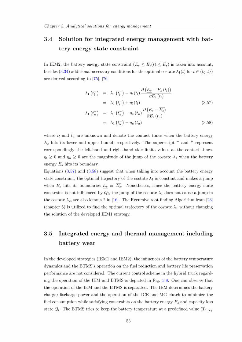
Chapter 3. Analytical solutions for energy management
3.4 Solution for integrated energy management with bat-
tery energy state constraint
In IEM2, the battery energy state constraint (Es ≤ Es(t) ≤ Es) is taken into account,
besides (3.34) additional necessary conditions for the optimal costate λ1(t) for t ∈ (t0, tf )
are derived according to [75], [76]
λ1
(t+l)
= λ1
(t−l)− ηl (tl)
∂(Es − Es (tl)
)∂Es (tl)
= λ1
(t−l)
+ ηl (tl) (3.57)
λ1
(t+u)
= λ1
(t−u)− ηu (tu)
∂(Es − Es
)∂Es (tu)
= λ1
(t−u)− ηu (tu) (3.58)
where tl and tu are unknown and denote the contact times when the battery energy
Es hits its lower and upper bound, respectively. The superscript − and + represent
correspondingly the left-hand and right-hand side limits values at the contact times.
ηl ≥ 0 and ηu ≥ 0 are the magnitude of the jump of the costate λ1 when the battery
energy Es hits its boundary.
Equations (3.57) and (3.58) suggest that when taking into account the battery energy
state constraint, the optimal trajectory of the costate λ1 is constant and makes a jump
when Es hits its boundaries Es or Es. Nonetheless, since the battery energy state
constraint is not influenced by Ql, the jump of the costate λ1 does not cause a jump in
the costate λ2, see also lemma 2 in [16]. The Recursive root finding Algorithm from [23]
(chapter 5) is utilized to find the optimal trajectory of the costate λ1 without changing
the solution of the developed IEM1 strategy.
3.5 Integrated energy and thermal management including
battery wear
In the developed strategies (IEM1 and IEM2), the influences of the battery temperature
dynamics and the BTMS’s operation on the fuel reduction and battery life preservation
performance are not considered. The current control scheme in the hybrid truck regard-
ing the operation of the IEM and BTMS is depicted in Fig. 3.8. One can observe that
the operation of the IEM and the BTMS is separated. The IEM determines the battery
charge/discharge power and the operation of the ICE and MG clutch to minimize the
fuel consumption while satisfying constraints on the battery energy Es and capacity loss
state Ql. The BTMS tries to keep the battery temperature at a predefined value (Tb ref
53
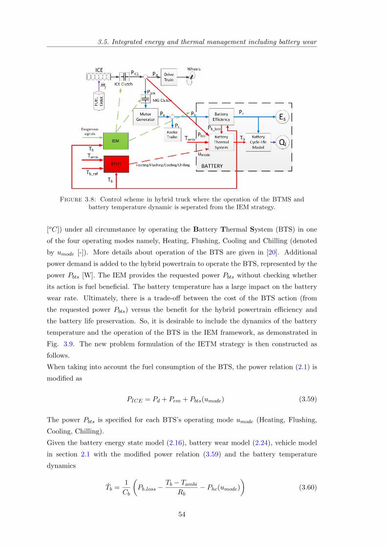
3.5. Integrated energy and thermal management including battery wear
Figure 3.8: Control scheme in hybrid truck where the operation of the BTMS andbattery temperature dynamic is seperated from the IEM strategy.
[oC]) under all circumstance by operating the Battery Thermal System (BTS) in one
of the four operating modes namely, Heating, Flushing, Cooling and Chilling (denoted
by umode [-]). More details about operation of the BTS are given in [20]. Additional
power demand is added to the hybrid powertrain to operate the BTS, represented by the
power Pbts [W]. The IEM provides the requested power Pbts without checking whether
its action is fuel beneficial. The battery temperature has a large impact on the battery
wear rate. Ultimately, there is a trade-off between the cost of the BTS action (from
the requested power Pbts) versus the benefit for the hybrid powertrain efficiency and
the battery life preservation. So, it is desirable to include the dynamics of the battery
temperature and the operation of the BTS in the IEM framework, as demonstrated in
Fig. 3.9. The new problem formulation of the IETM strategy is then constructed as
follows.
When taking into account the fuel consumption of the BTS, the power relation (2.1) is
modified as
PICE = Pd + Pem + Pbts(umode) (3.59)
The power Pbts is specified for each BTS’s operating mode umode (Heating, Flushing,
Cooling, Chilling).
Given the battery energy state model (2.16), battery wear model (2.24), vehicle model
in section 2.1 with the modified power relation (3.59) and the battery temperature
dynamics
Tb =1
Cb
(Pb loss −
Tb − TambiRb
− Phc(umode))
(3.60)
54
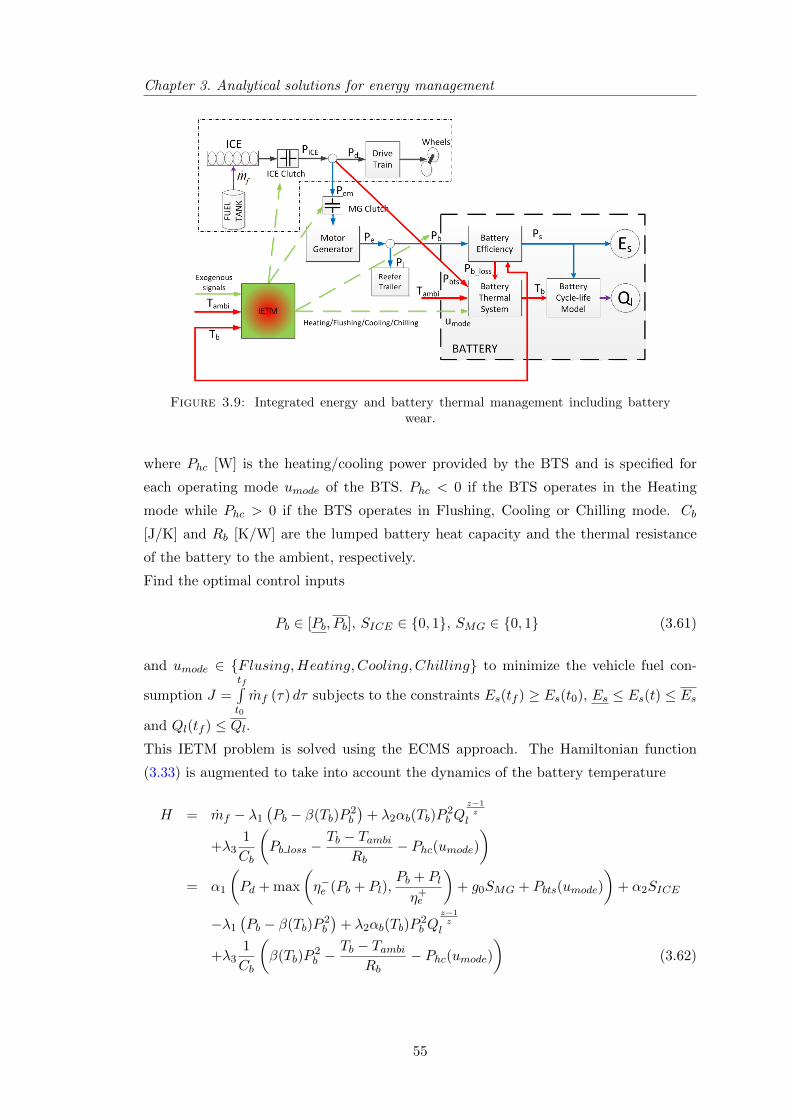
Chapter 3. Analytical solutions for energy management
Figure 3.9: Integrated energy and battery thermal management including batterywear.
where Phc [W] is the heating/cooling power provided by the BTS and is specified for
each operating mode umode of the BTS. Phc < 0 if the BTS operates in the Heating
mode while Phc > 0 if the BTS operates in Flushing, Cooling or Chilling mode. Cb
[J/K] and Rb [K/W] are the lumped battery heat capacity and the thermal resistance
of the battery to the ambient, respectively.
Find the optimal control inputs
Pb ∈ [Pb, Pb], SICE ∈ 0, 1, SMG ∈ 0, 1 (3.61)
and umode ∈ Flusing,Heating, Cooling, Chilling to minimize the vehicle fuel con-
sumption J =tf∫t0
mf (τ) dτ subjects to the constraints Es(tf ) ≥ Es(t0), Es ≤ Es(t) ≤ Es
and Ql(tf ) ≤ Ql.This IETM problem is solved using the ECMS approach. The Hamiltonian function
(3.33) is augmented to take into account the dynamics of the battery temperature
H = mf − λ1
(Pb − β(Tb)P
2b
)+ λ2αb(Tb)P
2b Q
z−1z
l
+λ31
Cb
(Pb loss −
Tb − TambiRb
− Phc(umode))
= α1
(Pd + max
(η−e (Pb + Pl),
Pb + Pl
η+e
)+ g0SMG + Pbts(umode)
)+ α2SICE
−λ1
(Pb − β(Tb)P
2b
)+ λ2αb(Tb)P
2b Q
z−1z
l
+λ31
Cb
(β(Tb)P
2b −
Tb − TambiRb
− Phc(umode))
(3.62)
55
3.6. Conclusions
Since there are six operating modes of the hybrid truck (ICE Only, PSM, MO, MA, C
and R) and four operating modes of the BTS (Heating, Flushing, Cooling and Chilling),
the Hamiltonian function (3.62) has 24 different formulations making it quite complex
to derive an analytical solution to the IETM strategy. Nevertheless, given the optimal
costates λo1, λo2, λo3 and other measured exogenous signals, minimization of the Hamil-
tonian function H(Pb, SICE , SMG, umode, λo1, λ
o2, λ
o3, t) (3.62) can still be computed by
numerically evaluating these 24 Hamiltonian functions on a dense grid. The optimal
hybrid truck operating mode is specified as the feasible mode which has the smallest
Hamiltonian function value among their 24 different formulations. Operations of the
BTS and the clutch system are specified accordingly. Verification of the IETM strategy
will be addressed in future research.
3.6 Conclusions
The fuel minimization OCPs (CEM1, CEM2, IEM1 and IEM2), defined in Table 1.2,
are addressed in this chapter. Without considering the battery life requirement, an ana-
lytical solution to CEM1 strategy, utilizing ECMS technique, is derived to minimize the
fuel consumption of the hybrid truck by controlling the battery charge/discharge power
and the clutch system’s operation. The analytical solution of the CEM1 strategy yields
the explicit operating regions of the hybrid truck operating mode. Moreover, analyzing
the analytical solution of the CEM1 reveals that decoupling the MG from the drivetrain
brings additional fuel benefit. The analytical solution of the CEM1 requires solving a
finite number of simple algebraic equations. It, therefore, results in a computationally-
efficient algorithm being applicable for real-life application. Without modifying the
explicit expressions in Table 3.2, the CEM2 strategy uses the solution of the CEM1 to
take into account also the battery energy state constraint (Es ≤ Es(t) ≤ Es).When considering the battery life requirement, the developed battery cycle-life model is
approximated by a convex function to be incorporated in the EMS framework. By ex-
ploiting the approximated model, the IEM1 strategy is formulated and solved explicitly
to minimize the vehicle fuel consumption while satisfying the battery capacity loss and
charge sustaining constraints. The IEM1 strategy makes use of the ECMS technique
and takes into account not only the battery energy but also the battery capacity loss
state in the Hamiltonian function. Henceforth, the IEM1 strategy is able to balance
three costs: the fuel consumption, the battery charge/discharge powers and the bat-
tery capacity loss. During driving periods, the optimal hybrid truck operating mode
and battery power are determined by searching the smallest (regarding the Hamiltonian
function’s value) feasible (regarding the battery power limitation (Pb ≤ Pb ≤ Pb)) mode
among five possible operating modes: ICE Only, PSM, MO, MA and C. The searching
56

Chapter 3. Analytical solutions for energy management
algorithm is done by solving a finite number of simple algebraic equations. It, therefore,
results in a computationally-efficient algorithm. Without modifying the explicit expres-
sions in Table 3.4, the IEM2 strategy uses the solution of the IEM1 to take into account
also the battery energy state constraint (Es ≤ Es(t) ≤ Es).The developed strategies (CEM1, CEM2, IEM1 and IEM2) requires the future informa-
tion of the driving cycle and battery temperature (kept at constant value) to find the
optimal control parameters. Although, this requirement leads to non-causal strategies,
the derived solutions provides a basis for developing a real-time implementable strategy,
presented in chapter 4.
57

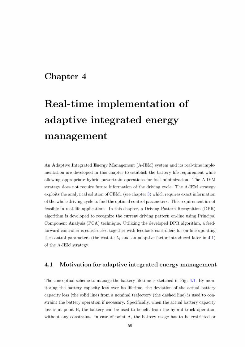
Chapter 4
Real-time implementation of
adaptive integrated energy
management
An Adaptive Integrated Energy Management (A-IEM) system and its real-time imple-
mentation are developed in this chapter to establish the battery life requirement while
allowing appropriate hybrid powertrain operations for fuel minimization. The A-IEM
strategy does not require future information of the driving cycle. The A-IEM strategy
exploits the analytical solution of CEM1 (see chapter 3) which requires exact information
of the whole driving cycle to find the optimal control parameters. This requirement is not
feasible in real-life applications. In this chapter, a Driving Pattern Recognition (DPR)
algorithm is developed to recognize the current driving pattern on-line using Principal
Component Analysis (PCA) technique. Utilizing the developed DPR algorithm, a feed-
forward controller is constructed together with feedback controllers for on-line updating
the control parameters (the costate λ1 and an adaptive factor introduced later in 4.1)
of the A-IEM strategy.
4.1 Motivation for adaptive integrated energy management
The conceptual scheme to manage the battery lifetime is sketched in Fig. 4.1. By mon-
itoring the battery capacity loss over its lifetime, the deviation of the actual battery
capacity loss (the solid line) from a nominal trajectory (the dashed line) is used to con-
straint the battery operation if necessary. Specifically, when the actual battery capacity
loss is at point B, the battery can be used to benefit from the hybrid truck operation
without any constraint. In case of point A, the battery usage has to be restricted or
59
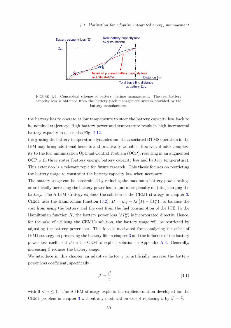
4.1. Motivation for adaptive integrated energy management
Figure 4.1: Conceptual scheme of battery lifetime management. The real batterycapacity loss is obtained from the battery pack management system provided by the
battery manufacturer.
the battery has to operate at low temperature to steer the battery capacity loss back to
its nominal trajectory. High battery power and temperature result in high incremental
battery capacity loss, see also Fig. 2.12.
Integrating the battery temperature dynamics and the associated BTMS operation in the
IEM may bring additional benefits and practically valuable. However, it adds complex-
ity to the fuel minimization Optimal Control Problem (OCP), resulting in an augmented
OCP with three states (battery energy, battery capacity loss and battery temperature).
This extension is a relevant topic for future research. This thesis focuses on restricting
the battery usage to constraint the battery capacity loss when necessary.
The battery usage can be constrained by reducing the maximum battery power ratings
or artificially increasing the battery power loss to put more penalty on (dis-)charging the
battery. The A-IEM strategy exploits the solution of the CEM1 strategy in chapter 3.
CEM1 uses the Hamiltonian function (3.2), H = mf − λ1
(Pb − βP 2
b
), to balance the
cost from using the battery and the cost from the fuel consumption of the ICE. In the
Hamiltonian function H, the battery power loss (βP 2b ) is incorporated directly. Hence,
for the sake of utilizing the CEM1’s solution, the battery usage will be restricted by
adjusting the battery power loss. This idea is motivated from analyzing the effect of
IEM1 strategy on preserving the battery life in chapter 3 and the influence of the battery
power loss coefficient β on the CEM1’s explicit solution in Appendix A.3. Generally,
increasing β reduces the battery usage.
We introduce in this chapter an adaptive factor γ to artificially increase the battery
power loss coefficient, specifically
β′
=β
γ(4.1)
with 0 < γ ≤ 1. The A-IEM strategy exploits the explicit solution developed for the
CEM1 problem in chapter 3 without any modification except replacing β by β′
= βγ .
60
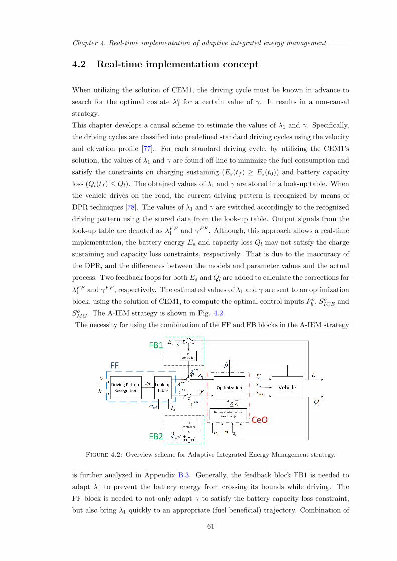
Chapter 4. Real-time implementation of adaptive integrated energy management
4.2 Real-time implementation concept
When utilizing the solution of CEM1, the driving cycle must be known in advance to
search for the optimal costate λo1 for a certain value of γ. It results in a non-causal
strategy.
This chapter develops a causal scheme to estimate the values of λ1 and γ. Specifically,
the driving cycles are classified into predefined standard driving cycles using the velocity
and elevation profile [77]. For each standard driving cycle, by utilizing the CEM1’s
solution, the values of λ1 and γ are found off-line to minimize the fuel consumption and
satisfy the constraints on charging sustaining (Es(tf ) ≥ Es(t0)) and battery capacity
loss (Ql(tf ) ≤ Ql). The obtained values of λ1 and γ are stored in a look-up table. When
the vehicle drives on the road, the current driving pattern is recognized by means of
DPR techniques [78]. The values of λ1 and γ are switched accordingly to the recognized
driving pattern using the stored data from the look-up table. Output signals from the
look-up table are denoted as λFF1 and γFF . Although, this approach allows a real-time
implementation, the battery energy Es and capacity loss Ql may not satisfy the charge
sustaining and capacity loss constraints, respectively. That is due to the inaccuracy of
the DPR, and the differences between the models and parameter values and the actual
process. Two feedback loops for both Es and Ql are added to calculate the corrections for
λFF1 and γFF , respectively. The estimated values of λ1 and γ are sent to an optimization
block, using the solution of CEM1, to compute the optimal control inputs P ob , SoICE and
SoMG. The A-IEM strategy is shown in Fig. 4.2.
The necessity for using the combination of the FF and FB blocks in the A-IEM strategy
Figure 4.2: Overview scheme for Adaptive Integrated Energy Management strategy.
is further analyzed in Appendix B.3. Generally, the feedback block FB1 is needed to
adapt λ1 to prevent the battery energy from crossing its bounds while driving. The
FF block is needed to not only adapt γ to satisfy the battery capacity loss constraint,
but also bring λ1 quickly to an appropriate (fuel beneficial) trajectory. Combination of
61
4.2. Real-time implementation concept
the FF and FB blocks results in a reliable solution for satisfying the constraints while
achieving minimal fuel consumption.
The A-IEM strategy consists of a Feedforward (FF, denoted by dash line) control block,
two Feedback (FB1 and FB2, denoted by dotted line) control blocks and an Cost-effective
Optimization (CeO, denoted by dash-dot-dot line) block. The main functions of these
blocks are briefly explained as follows:
• The FF control block is constructed from a DPR and Look-up table layer. The
DPR layer classifies the current driving pattern using the information of the vehicle
velocity v and the road elevation h. The Look-up table layer stores the off-line
calculated values of λ1 and γ for different driving scenarios with respect to the
driving pattern (denoted by dp) and the measured vehicle mass mveh, battery
temperature Tb, see Fig. 4.3. It is noteworthy that mveh impacts on the driver
Figure 4.3: Optimal values of λ1 and γ for a certain mveh and various values of Tbfor City flat and City hilly driving cycles.
power demand and Tb influences the battery power loss coefficient. mveh and
Tb ultimately influence λ1 and γ. With the detected dp and the look-up table,
appropriate values of λFF1 and γFF become available. The DPR layer is presented
in details in subsection 4.3.
• FB control blocks: The FB control blocks utilize each a PI controller to correct
the feedforward signals λFF1 and γFF to regulate the actual battery energy Es
and actual capacity loss Ql around their specified reference signals Es ref and
Ql ref , respectively (see Fig. 4.2). Subsection 4.4 discusses the tuning of both PI
controllers.
• CeO block: In the CeO block, the Optimization layer outputs the optimal control
inputs P ob , SoICE and SoMG using the explicit solution of CEM1 with the estimated
λ1 and γ from the FB1, FB2 and FF control blocks. The Battery Cost-effective
62
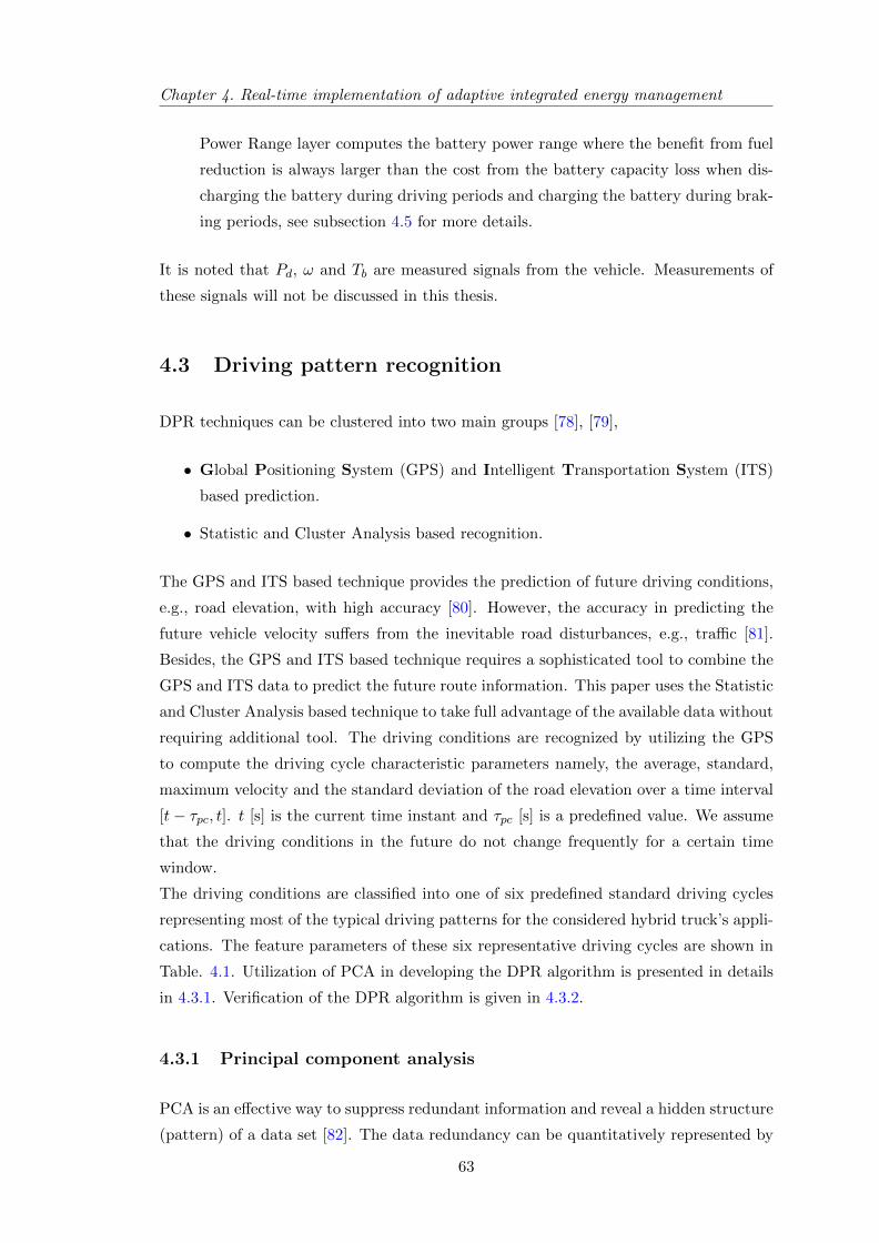
Chapter 4. Real-time implementation of adaptive integrated energy management
Power Range layer computes the battery power range where the benefit from fuel
reduction is always larger than the cost from the battery capacity loss when dis-
charging the battery during driving periods and charging the battery during brak-
ing periods, see subsection 4.5 for more details.
It is noted that Pd, ω and Tb are measured signals from the vehicle. Measurements of
these signals will not be discussed in this thesis.
4.3 Driving pattern recognition
DPR techniques can be clustered into two main groups [78], [79],
• Global Positioning System (GPS) and Intelligent Transportation System (ITS)
based prediction.
• Statistic and Cluster Analysis based recognition.
The GPS and ITS based technique provides the prediction of future driving conditions,
e.g., road elevation, with high accuracy [80]. However, the accuracy in predicting the
future vehicle velocity suffers from the inevitable road disturbances, e.g., traffic [81].
Besides, the GPS and ITS based technique requires a sophisticated tool to combine the
GPS and ITS data to predict the future route information. This paper uses the Statistic
and Cluster Analysis based technique to take full advantage of the available data without
requiring additional tool. The driving conditions are recognized by utilizing the GPS
to compute the driving cycle characteristic parameters namely, the average, standard,
maximum velocity and the standard deviation of the road elevation over a time interval
[t− τpc, t]. t [s] is the current time instant and τpc [s] is a predefined value. We assume
that the driving conditions in the future do not change frequently for a certain time
window.
The driving conditions are classified into one of six predefined standard driving cycles
representing most of the typical driving patterns for the considered hybrid truck’s appli-
cations. The feature parameters of these six representative driving cycles are shown in
Table. 4.1. Utilization of PCA in developing the DPR algorithm is presented in details
in 4.3.1. Verification of the DPR algorithm is given in 4.3.2.
4.3.1 Principal component analysis
PCA is an effective way to suppress redundant information and reveal a hidden structure
(pattern) of a data set [82]. The data redundancy can be quantitatively represented by
63
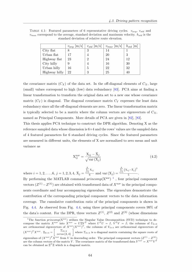
4.3. Driving pattern recognition
Table 4.1: Featured parameters of 6 representative driving cycles. vavg, vstd andvmax correspond to the average, standard deviation and maximum velocity. hstd is the
standard deviation of relative route elevation.
vavg [m/s] vstd [m/s] vmax [m/s] hstd [m]
City flat 8 3 14 1Urban flat 17 4 20 3Highway flat 23 2 24 12City hilly 9 4 16 30Urban hilly 16 5 22 32Highway hilly 22 3 25 40
the covariance matrix (CX) of the data set. In the off-diagonal elements of CX , large
(small) values correspond to high (low) data redundancy [83]. PCA aims at finding a
linear transformation to transform the original data set to a new one whose covariance
matrix (CY ) is diagonal. The diagonal covariance matrix CY expresses the least data
redundancy since all the off-diagonal elements are zero. The linear transformation matrix
is typically selected to be a matrix where the column vectors are eigenvectors of CX ,
named as Principal Components. More details of PCA are given in [82], [83].
This thesis applies PCA technique to construct the DPR algorithm. Denoting X as the
reference sampled data whose dimension is 6×4 and the rows’ values are the sampled data
of 4 featured parameters for 6 standard driving cycles. Since the featured parameters
are measured in different units, the elements of X are normalized to zero mean and unit
variance as
Xnorij =
Xij − Xj√var (Xj)
(4.2)
where i = 1, 2, . . . , 6, j = 1, 2, 3, 4, Xj =
6∑i=1
Xij
6 and var (Xj) =
6∑i=1
(Xij−Xj)2
5 .
By performing the MATLAB command princomp(Xnor) 1 , four principal component
vectors (Z(1)−Z(4)) are obtained with transformed data of Xnor in the principal compo-
nents coordinate and four accompanying eigenvalues. The eigenvalues demonstrate the
contribution of the corresponding principal component vectors to the data information
coverage. The cumulative contribution ratio of the principal components is shown in
Fig. 4.4. As observed from Fig. 4.4, using three principal components covers 99% of
the data’s content. For the DPR, three vectors Z(1), Z(2) and Z(3) (whose dimensions
1The function princomp(Xnor) utilizes the Singular Value Decomposition (SVD) technique to de-compose the matrix Xnor into Xnor = UΞV T where UTU = I, V TV = I; the columns of U6×6
are orthonormal eigenvectors of Xnor(Xnor)T , the columns of V4×4 are orthonormal eigenvectors of
(Xnor)TXnor. Ξ6×4 =
[Σ4×4
zeros (2, 4)
]where Σ4×4 is a diagonal matrix containing the square roots of
eigenvalues of (Xnor)TXnor from V in descending order. The principal component vectors (Z(1) −Z(4))are the column vectors of the matrix V . The covariance matrix of the transformed data Y nor = XnorV T
can be obtained as ΞTΞ which is a diagonal matrix.
64
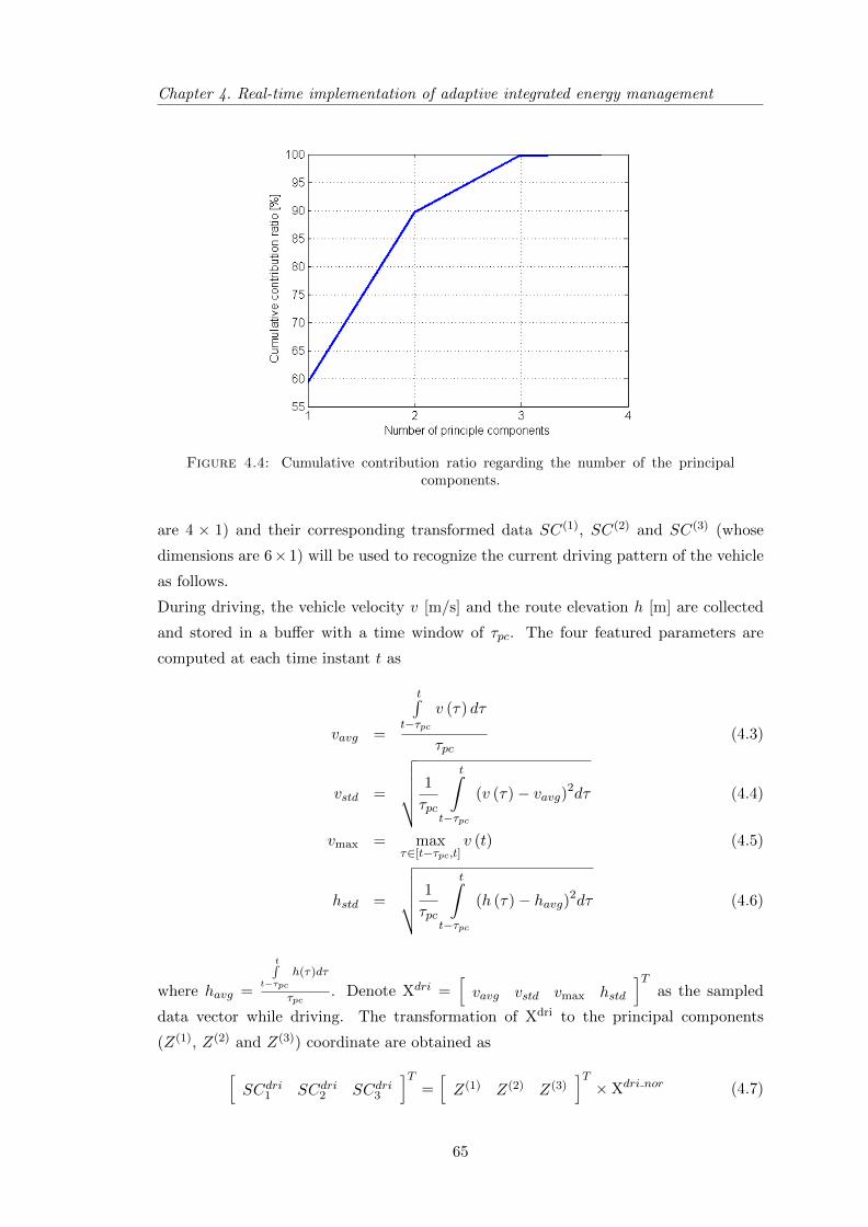
Chapter 4. Real-time implementation of adaptive integrated energy management
Figure 4.4: Cumulative contribution ratio regarding the number of the principalcomponents.
are 4 × 1) and their corresponding transformed data SC(1), SC(2) and SC(3) (whose
dimensions are 6×1) will be used to recognize the current driving pattern of the vehicle
as follows.
During driving, the vehicle velocity v [m/s] and the route elevation h [m] are collected
and stored in a buffer with a time window of τpc. The four featured parameters are
computed at each time instant t as
vavg =
t∫t−τpc
v (τ) dτ
τpc(4.3)
vstd =
√√√√√ 1
τpc
t∫t−τpc
(v (τ)− vavg)2dτ (4.4)
vmax = maxτ∈[t−τpc,t]
v (t) (4.5)
hstd =
√√√√√ 1
τpc
t∫t−τpc
(h (τ)− havg)2dτ (4.6)
where havg =
t∫t−τpc
h(τ)dτ
τpc. Denote Xdri =
[vavg vstd vmax hstd
]Tas the sampled
data vector while driving. The transformation of Xdri to the principal components
(Z(1), Z(2) and Z(3)) coordinate are obtained as[SCdri1 SCdri2 SCdri3
]T=[Z(1) Z(2) Z(3)
]T×Xdri nor (4.7)
65
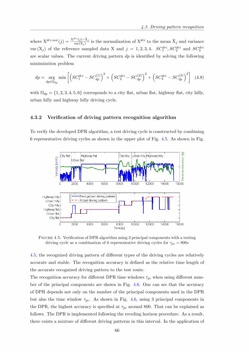
4.3. Driving pattern recognition
where Xdri nor(j) =Xdri(j)−Xj
var(Xj)is the normalization of Xdri to the mean Xj and variance
var (Xj) of the reference sampled data X and j = 1, 2, 3, 4. SCdri1 , SCdri2 and SCdri3
are scalar values. The current driving pattern dp is identified by solving the following
minimization problem
dp = argdp∈Ωdp
min
[(SCdri1 − SC(1)
dp
)2+(SCdri2 − SC(2)
dp
)2+(SCdri3 − SC(3)
dp
)2]
(4.8)
with Ωdp = 1, 2, 3, 4, 5, 6 corresponds to a city flat, urban flat, highway flat, city hilly,
urban hilly and highway hilly driving cycle.
4.3.2 Verification of driving pattern recognition algorithm
To verify the developed DPR algorithm, a test driving cycle is constructed by combining
6 representative driving cycles as shown in the upper plot of Fig. 4.5. As shown in Fig.
Figure 4.5: Verification of DPR algorithm using 3 principal components with a testingdriving cycle as a combination of 6 representative driving cycles for τpc = 800s
4.5, the recognized driving pattern of different types of the driving cycles are relatively
accurate and stable. The recognition accuracy is defined as the relative time length of
the accurate recognized driving pattern to the test route.
The recognition accuracy for different DPR time windows τpc when using different num-
ber of the principal components are shown in Fig. 4.6. One can see that the accuracy
of DPR depends not only on the number of the principal components used in the DPR
but also the time window τpc. As shown in Fig. 4.6, using 3 principal components in
the DPR, the highest accuracy is specified at τpc around 800. That can be explained as
follows. The DPR is implemented following the receding horizon procedure. As a result,
there exists a mixture of different driving patterns in this interval. In the application of
66
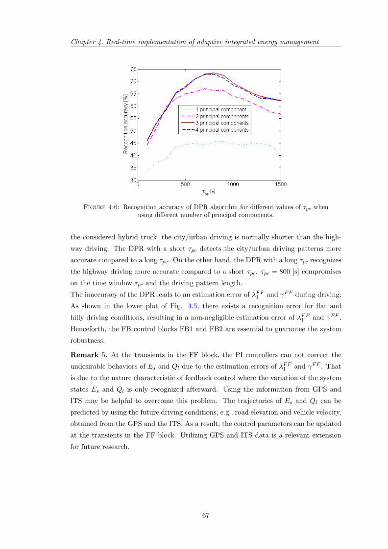
Chapter 4. Real-time implementation of adaptive integrated energy management
Figure 4.6: Recognition accuracy of DPR algorithm for different values of τpc whenusing different number of principal components.
the considered hybrid truck, the city/urban driving is normally shorter than the high-
way driving. The DPR with a short τpc detects the city/urban driving patterns more
accurate compared to a long τpc. On the other hand, the DPR with a long τpc recognizes
the highway driving more accurate compared to a short τpc. τpc = 800 [s] compromises
on the time window τpc and the driving pattern length.
The inaccuracy of the DPR leads to an estimation error of λFF1 and γFF during driving.
As shown in the lower plot of Fig. 4.5, there exists a recognition error for flat and
hilly driving conditions, resulting in a non-negligible estimation error of λFF1 and γFF .
Henceforth, the FB control blocks FB1 and FB2 are essential to guarantee the system
robustness.
Remark 5. At the transients in the FF block, the PI controllers can not correct the
undesirable behaviors of Es and Ql due to the estimation errors of λFF1 and γFF . That
is due to the nature characteristic of feedback control where the variation of the system
states Es and Ql is only recognized afterward. Using the information from GPS and
ITS may be helpful to overcome this problem. The trajectories of Es and Ql can be
predicted by using the future driving conditions, e.g., road elevation and vehicle velocity,
obtained from the GPS and the ITS. As a result, the control parameters can be updated
at the transients in the FF block. Utilizing GPS and ITS data is a relevant extension
for future research.
67
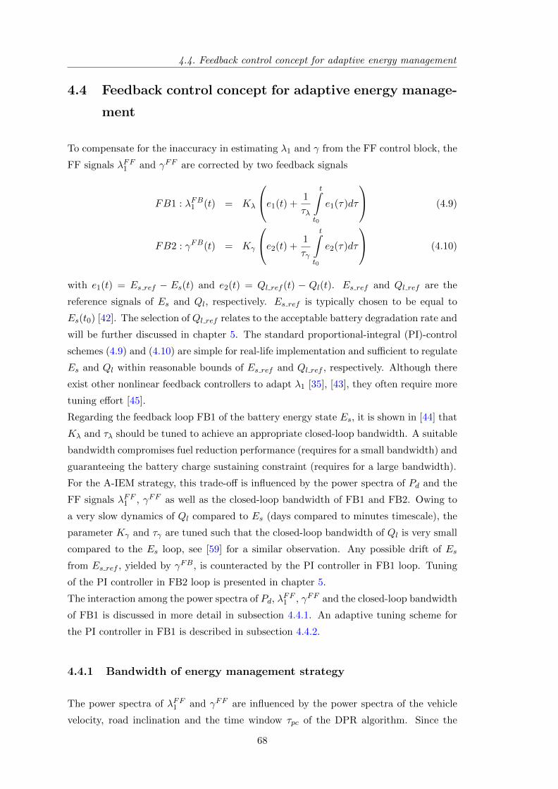
4.4. Feedback control concept for adaptive energy management
4.4 Feedback control concept for adaptive energy manage-
ment
To compensate for the inaccuracy in estimating λ1 and γ from the FF control block, the
FF signals λFF1 and γFF are corrected by two feedback signals
FB1 : λFB1 (t) = Kλ
e1(t) +1
τλ
t∫t0
e1(τ)dτ
(4.9)
FB2 : γFB(t) = Kγ
e2(t) +1
τγ
t∫t0
e2(τ)dτ
(4.10)
with e1(t) = Es ref − Es(t) and e2(t) = Ql ref (t) − Ql(t). Es ref and Ql ref are the
reference signals of Es and Ql, respectively. Es ref is typically chosen to be equal to
Es(t0) [42]. The selection of Ql ref relates to the acceptable battery degradation rate and
will be further discussed in chapter 5. The standard proportional-integral (PI)-control
schemes (4.9) and (4.10) are simple for real-life implementation and sufficient to regulate
Es and Ql within reasonable bounds of Es ref and Ql ref , respectively. Although there
exist other nonlinear feedback controllers to adapt λ1 [35], [43], they often require more
tuning effort [45].
Regarding the feedback loop FB1 of the battery energy state Es, it is shown in [44] that
Kλ and τλ should be tuned to achieve an appropriate closed-loop bandwidth. A suitable
bandwidth compromises fuel reduction performance (requires for a small bandwidth) and
guaranteeing the battery charge sustaining constraint (requires for a large bandwidth).
For the A-IEM strategy, this trade-off is influenced by the power spectra of Pd and the
FF signals λFF1 , γFF as well as the closed-loop bandwidth of FB1 and FB2. Owing to
a very slow dynamics of Ql compared to Es (days compared to minutes timescale), the
parameter Kγ and τγ are tuned such that the closed-loop bandwidth of Ql is very small
compared to the Es loop, see [59] for a similar observation. Any possible drift of Es
from Es ref , yielded by γFB, is counteracted by the PI controller in FB1 loop. Tuning
of the PI controller in FB2 loop is presented in chapter 5.
The interaction among the power spectra of Pd, λFF1 , γFF and the closed-loop bandwidth
of FB1 is discussed in more detail in subsection 4.4.1. An adaptive tuning scheme for
the PI controller in FB1 is described in subsection 4.4.2.
4.4.1 Bandwidth of energy management strategy
The power spectra of λFF1 and γFF are influenced by the power spectra of the vehicle
velocity, road inclination and the time window τpc of the DPR algorithm. Since the
68
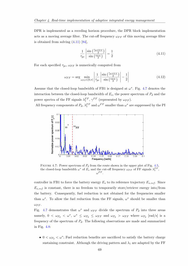
Chapter 4. Real-time implementation of adaptive integrated energy management
DPR is implemented as a receding horizon procedure, the DPR block implementation
acts as a moving average filter. The cut-off frequency ωFF of this moving average filter
is obtained from solving (4.11) [84],
1
τpc
∣∣∣∣∣sin( τpcωFF
2
)sin(ωFF
2
) ∣∣∣∣∣ =1
2(4.11)
For each specified τpc, ωFF is numerically computed from
ωFF = arg minωFF∈[0,π]
∣∣∣∣∣ 1
τpc
∣∣∣∣∣sin( τpcωFF
2
)sin(ωFF
2
) ∣∣∣∣∣− 1
2
∣∣∣∣∣ (4.12)
Assume that the closed-loop bandwidth of FB1 is designed at ω∗. Fig. 4.7 denotes the
interaction between the closed-loop bandwidth of Es, the power spectrum of Pd and the
power spectra of the FF signals λFF1 , γFF (represented by ωFF ).
All frequency components of Pd, λFF1 and ωFF smaller than ω∗ are suppressed by the PI
Figure 4.7: Power spectrum of Pd from the route shown in the upper plot of Fig. 4.5,the closed-loop bandwidth ω∗ of Es and the cut-off frequency ωFF of FF signals λFF1 ,
ωFF .
controller in FB1 to force the battery energy Es to its reference trajectory Es ref . Since
Es ref is constant, there is no freedom to temporarily store/retrieve energy into/from
the battery. Consequently, fuel reduction is not obtained for the frequencies smaller
than ω∗. To allow the fuel reduction from the FF signals, ω∗ should be smaller than
ωFF .
Fig. 4.7 demonstrates that ω∗ and ωFF divide the spectrum of Pd into three areas
namely, 0 < ωPd < ω∗, ω∗ ≤ ωPd ≤ ωFF and ωPd > ωFF where ωPd [rad/s] is a
frequency of the spectrum of Pd. The following observations are made and summarized
in Fig. 4.8:
• 0 < ωPd < ω∗; Fuel reduction benefits are sacrificed to satisfy the battery charge
sustaining constraint. Although the driving pattern and λ1 are adapted by the FF
69
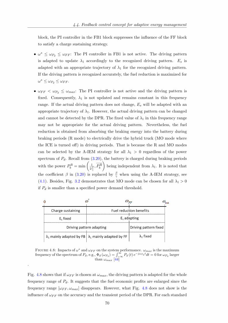
4.4. Feedback control concept for adaptive energy management
block, the PI controller in the FB1 block suppresses the influence of the FF block
to satisfy a charge sustaining strategy.
• ω∗ ≤ ωPd ≤ ωFF : The PI controller in FB1 is not active. The driving pattern
is adapted to update λ1 accordingly to the recognized driving pattern. Es is
adapted with an appropriate trajectory of λ1 for the recognized driving pattern.
If the driving pattern is recognized accurately, the fuel reduction is maximized for
ω∗ ≤ ωPd ≤ ωFF .
• ωFF < ωPd ≤ ωmax: The PI controller is not active and the driving pattern is
fixed. Consequently, λ1 is not updated and remains constant in this frequency
range. If the actual driving pattern does not change, Es will be adapted with an
appropriate trajectory of λ1. However, the actual driving pattern can be changed
and cannot be detected by the DPR. The fixed value of λ1 in this frequency range
may not be appropriate for the actual driving pattern. Nevertheless, the fuel
reduction is obtained from absorbing the braking energy into the battery during
braking periods (R mode) to electrically drive the hybrid truck (MO mode where
the ICE is turned off) in driving periods. That is because the R and MO modes
can be selected by the A-IEM strategy for all λ1 > 0 regardless of the power
spectrum of Pd. Recall from (3.20), the battery is charged during braking periods
with the power PRb = min
(1
2βγ
, PRb
)being independent from λ1. It is noted that
the coefficient β in (3.20) is replaced by βγ when using the A-IEM strategy, see
(4.1). Besides, Fig. 3.2 demonstrates that MO mode can be chosen for all λ1 > 0
if Pd is smaller than a specified power demand threshold.
Figure 4.8: Impacts of ω∗ and ωFF on the system performance. ωmax is the maximumfrequency of the spectrum of Pd, e.g., Φd (ωPd
) =∫∞−∞ Pd (t) e−jωPd
tdt = 0 for ωPdlarger
than ωmax [44]
.
Fig. 4.8 shows that if ωFF is chosen at ωmax, the driving pattern is adapted for the whole
frequency range of Pd. It suggests that the fuel economic profits are enlarged since the
frequency range [ωFF , ωmax] disappears. However, what Fig. 4.8 does not show is the
influence of ωFF on the accuracy and the transient period of the DPR. For each standard
70
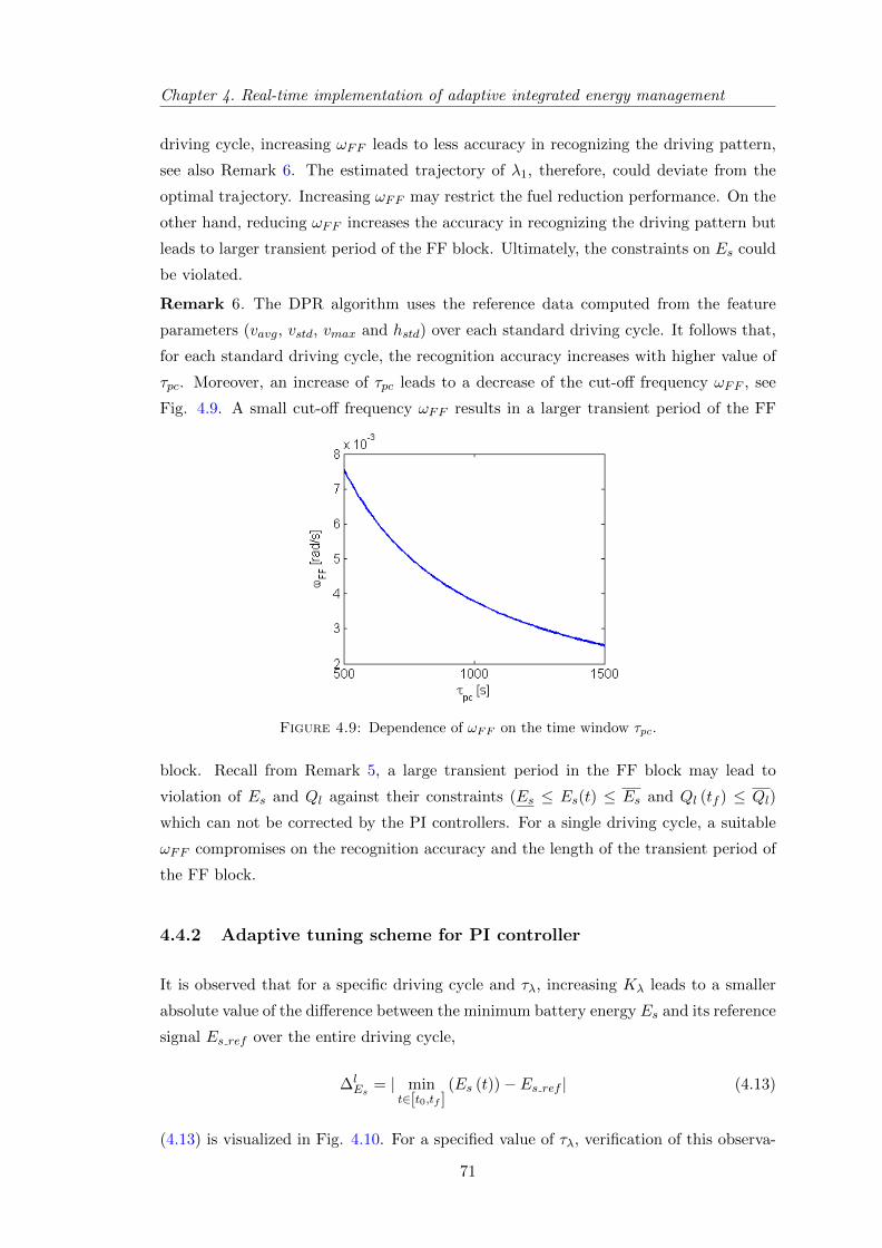
Chapter 4. Real-time implementation of adaptive integrated energy management
driving cycle, increasing ωFF leads to less accuracy in recognizing the driving pattern,
see also Remark 6. The estimated trajectory of λ1, therefore, could deviate from the
optimal trajectory. Increasing ωFF may restrict the fuel reduction performance. On the
other hand, reducing ωFF increases the accuracy in recognizing the driving pattern but
leads to larger transient period of the FF block. Ultimately, the constraints on Es could
be violated.
Remark 6. The DPR algorithm uses the reference data computed from the feature
parameters (vavg, vstd, vmax and hstd) over each standard driving cycle. It follows that,
for each standard driving cycle, the recognition accuracy increases with higher value of
τpc. Moreover, an increase of τpc leads to a decrease of the cut-off frequency ωFF , see
Fig. 4.9. A small cut-off frequency ωFF results in a larger transient period of the FF
Figure 4.9: Dependence of ωFF on the time window τpc.
block. Recall from Remark 5, a large transient period in the FF block may lead to
violation of Es and Ql against their constraints (Es ≤ Es(t) ≤ Es and Ql (tf ) ≤ Ql)
which can not be corrected by the PI controllers. For a single driving cycle, a suitable
ωFF compromises on the recognition accuracy and the length of the transient period of
the FF block.
4.4.2 Adaptive tuning scheme for PI controller
It is observed that for a specific driving cycle and τλ, increasing Kλ leads to a smaller
absolute value of the difference between the minimum battery energy Es and its reference
signal Es ref over the entire driving cycle,
∆lEs = | min
t∈[t0,tf ](Es (t))− Es ref | (4.13)
(4.13) is visualized in Fig. 4.10. For a specified value of τλ, verification of this observa-
71
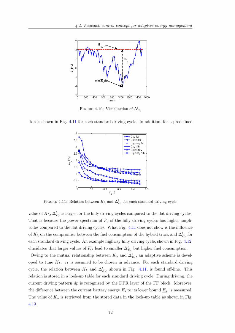
4.4. Feedback control concept for adaptive energy management
Figure 4.10: Visualization of ∆lEs
tion is shown in Fig. 4.11 for each standard driving cycle. In addition, for a predefined
Figure 4.11: Relation between Kλ and ∆lEs
for each standard driving cycle.
value of Kλ, ∆lEs
is larger for the hilly driving cycles compared to the flat driving cycles.
That is because the power spectrum of Pd of the hilly driving cycles has higher ampli-
tudes compared to the flat driving cycles. What Fig. 4.11 does not show is the influence
of Kλ on the compromise between the fuel consumption of the hybrid truck and ∆lEs
for
each standard driving cycle. An example highway hilly driving cycle, shown in Fig. 4.12,
elucidates that larger values of Kλ lead to smaller ∆lEs
but higher fuel consumption.
Owing to the mutual relationship between Kλ and ∆lEs
, an adaptive scheme is devel-
oped to tune Kλ. τλ is assumed to be chosen in advance. For each standard driving
cycle, the relation between Kλ and ∆lEs
, shown in Fig. 4.11, is found off-line. This
relation is stored in a look-up table for each standard driving cycle. During driving, the
current driving pattern dp is recognized by the DPR layer of the FF block. Moreover,
the difference between the current battery energy Es to its lower bound Es, is measured.
The value of Kλ is retrieved from the stored data in the look-up table as shown in Fig.
4.13.
72
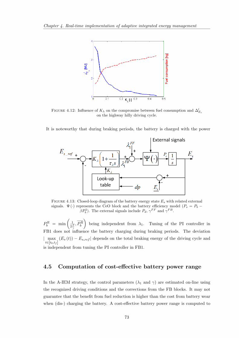
Chapter 4. Real-time implementation of adaptive integrated energy management
Figure 4.12: Influence of Kλ on the compromise between fuel consumption and ∆lEs
on the highway hilly driving cycle.
It is noteworthy that during braking periods, the battery is charged with the power
Figure 4.13: Closed-loop diagram of the battery energy state Es with related externalsignals. Ψ (·) represents the CeO block and the battery efficiency model (Ps = Pb −
βP 2b ). The external signals include Pd, γ
FF and γFB .
PRb = min
(1
2βγ
, PRb
)being independent from λ1. Tuning of the PI controller in
FB1 does not influence the battery charging during braking periods. The deviation
| maxt∈[t0,tf ]
(Es (t)) − Es ref | depends on the total braking energy of the driving cycle and
is independent from tuning the PI controller in FB1.
4.5 Computation of cost-effective battery power range
In the A-IEM strategy, the control parameters (λ1 and γ) are estimated on-line using
the recognized driving conditions and the corrections from the FB blocks. It may not
guarantee that the benefit from fuel reduction is higher than the cost from battery wear
when (dis-) charging the battery. A cost-effective battery power range is computed to
73
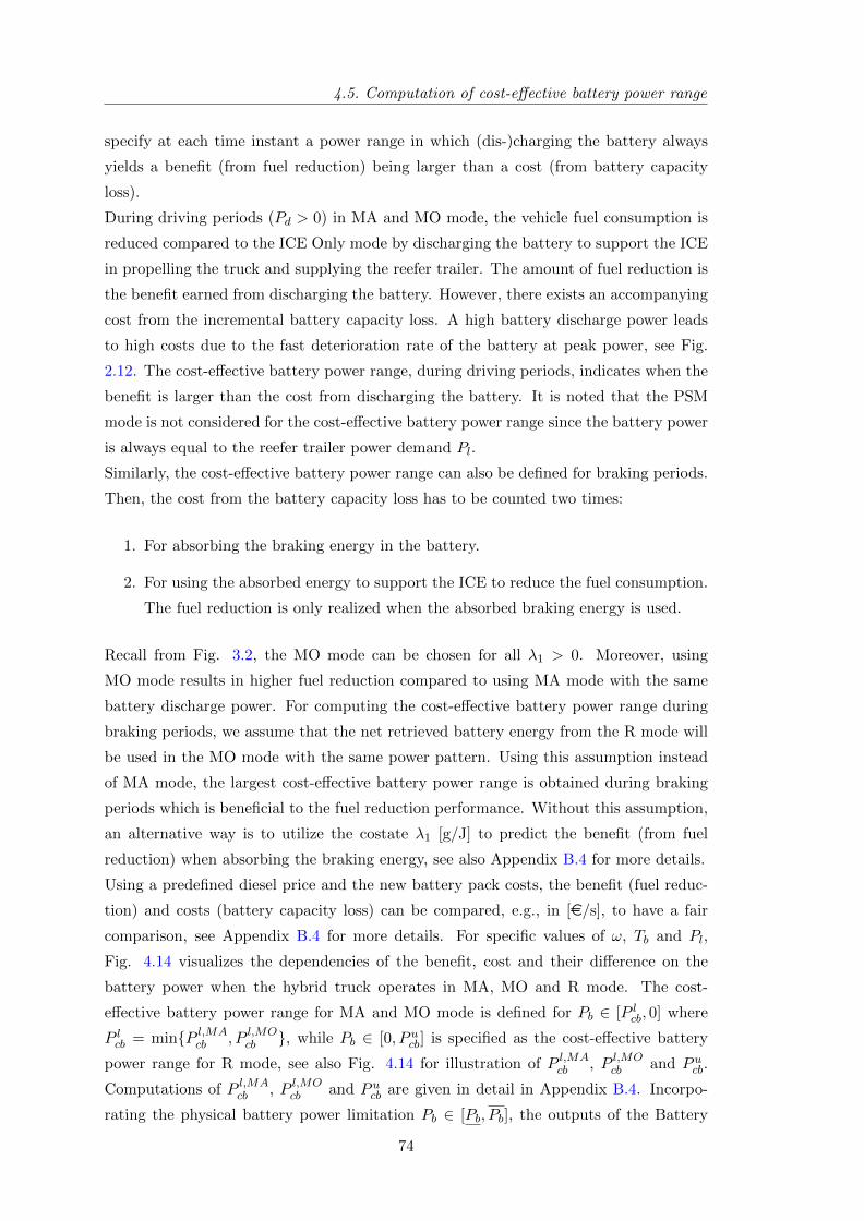
4.5. Computation of cost-effective battery power range
specify at each time instant a power range in which (dis-)charging the battery always
yields a benefit (from fuel reduction) being larger than a cost (from battery capacity
loss).
During driving periods (Pd > 0) in MA and MO mode, the vehicle fuel consumption is
reduced compared to the ICE Only mode by discharging the battery to support the ICE
in propelling the truck and supplying the reefer trailer. The amount of fuel reduction is
the benefit earned from discharging the battery. However, there exists an accompanying
cost from the incremental battery capacity loss. A high battery discharge power leads
to high costs due to the fast deterioration rate of the battery at peak power, see Fig.
2.12. The cost-effective battery power range, during driving periods, indicates when the
benefit is larger than the cost from discharging the battery. It is noted that the PSM
mode is not considered for the cost-effective battery power range since the battery power
is always equal to the reefer trailer power demand Pl.
Similarly, the cost-effective battery power range can also be defined for braking periods.
Then, the cost from the battery capacity loss has to be counted two times:
1. For absorbing the braking energy in the battery.
2. For using the absorbed energy to support the ICE to reduce the fuel consumption.
The fuel reduction is only realized when the absorbed braking energy is used.
Recall from Fig. 3.2, the MO mode can be chosen for all λ1 > 0. Moreover, using
MO mode results in higher fuel reduction compared to using MA mode with the same
battery discharge power. For computing the cost-effective battery power range during
braking periods, we assume that the net retrieved battery energy from the R mode will
be used in the MO mode with the same power pattern. Using this assumption instead
of MA mode, the largest cost-effective battery power range is obtained during braking
periods which is beneficial to the fuel reduction performance. Without this assumption,
an alternative way is to utilize the costate λ1 [g/J] to predict the benefit (from fuel
reduction) when absorbing the braking energy, see also Appendix B.4 for more details.
Using a predefined diesel price and the new battery pack costs, the benefit (fuel reduc-
tion) and costs (battery capacity loss) can be compared, e.g., in [e/s], to have a fair
comparison, see Appendix B.4 for more details. For specific values of ω, Tb and Pl,
Fig. 4.14 visualizes the dependencies of the benefit, cost and their difference on the
battery power when the hybrid truck operates in MA, MO and R mode. The cost-
effective battery power range for MA and MO mode is defined for Pb ∈ [P lcb, 0] where
P lcb = minP l,MAcb , P l,MO
cb , while Pb ∈ [0, P ucb] is specified as the cost-effective battery
power range for R mode, see also Fig. 4.14 for illustration of P l,MAcb , P l,MO
cb and P ucb.
Computations of P l,MAcb , P l,MO
cb and P ucb are given in detail in Appendix B.4. Incorpo-
rating the physical battery power limitation Pb ∈ [Pb, Pb], the outputs of the Battery
74
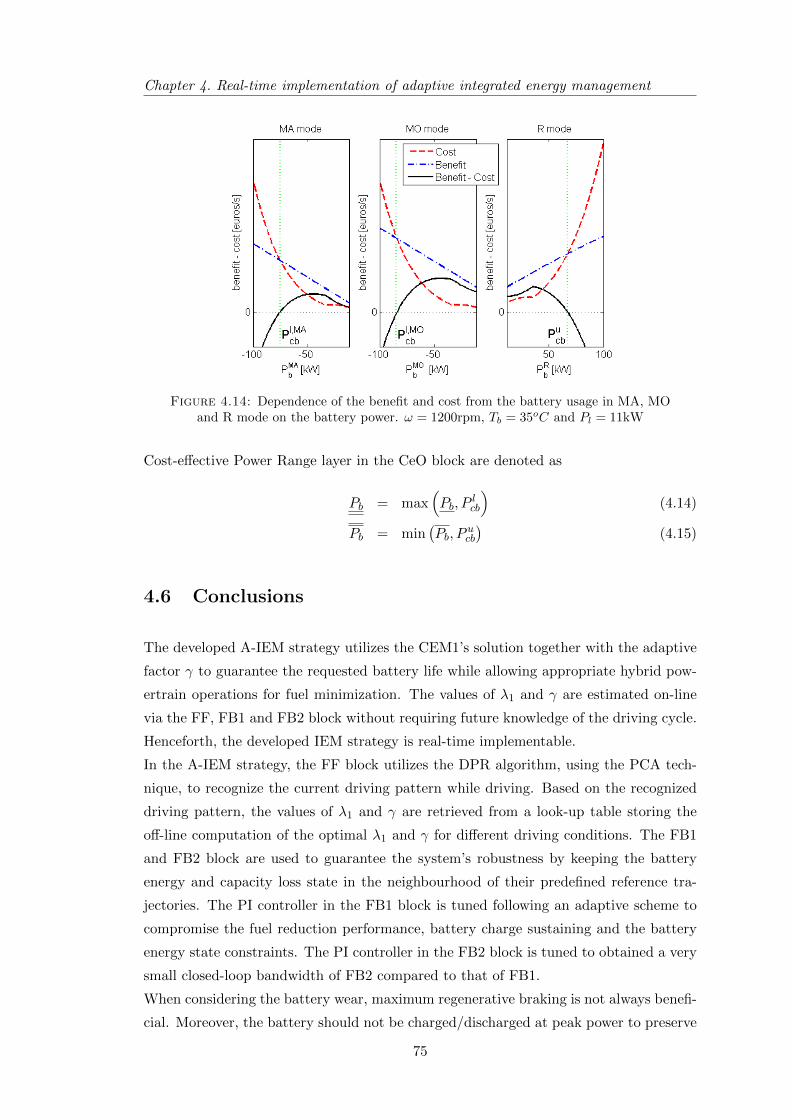
Chapter 4. Real-time implementation of adaptive integrated energy management
Figure 4.14: Dependence of the benefit and cost from the battery usage in MA, MOand R mode on the battery power. ω = 1200rpm, Tb = 35oC and Pl = 11kW
Cost-effective Power Range layer in the CeO block are denoted as
Pb = max(Pb, P
lcb
)(4.14)
Pb = min(Pb, P
ucb
)(4.15)
4.6 Conclusions
The developed A-IEM strategy utilizes the CEM1’s solution together with the adaptive
factor γ to guarantee the requested battery life while allowing appropriate hybrid pow-
ertrain operations for fuel minimization. The values of λ1 and γ are estimated on-line
via the FF, FB1 and FB2 block without requiring future knowledge of the driving cycle.
Henceforth, the developed IEM strategy is real-time implementable.
In the A-IEM strategy, the FF block utilizes the DPR algorithm, using the PCA tech-
nique, to recognize the current driving pattern while driving. Based on the recognized
driving pattern, the values of λ1 and γ are retrieved from a look-up table storing the
off-line computation of the optimal λ1 and γ for different driving conditions. The FB1
and FB2 block are used to guarantee the system’s robustness by keeping the battery
energy and capacity loss state in the neighbourhood of their predefined reference tra-
jectories. The PI controller in the FB1 block is tuned following an adaptive scheme to
compromise the fuel reduction performance, battery charge sustaining and the battery
energy state constraints. The PI controller in the FB2 block is tuned to obtained a very
small closed-loop bandwidth of FB2 compared to that of FB1.
When considering the battery wear, maximum regenerative braking is not always benefi-
cial. Moreover, the battery should not be charged/discharged at peak power to preserve
75

4.6. Conclusions
the battery life by avoiding high deterioration of its capacity. A cost-effective battery
power range is computed to specify at each time instant a power range in which (dis-)
charging the battery always yields a benefit (from fuel reduction) being larger than a
cost (from battery capacity loss).
76
Chapter 5
Simulation results
In this chapter, simulations are used to elucidate the benefits of the proposed energy
management strategies from chapter 3 and 4. Chapter 3 presented the solutions for
managing the power split between the ICE and MG to minimize the fuel consumption
without and with considering the battery life requirement. The derived solutions are
analytical. They provide the insight into:
• the benefit of using an additional MG clutch in the considered hybrid truck,
• the trade-off between the fuel reduction performance and battery life preservation
This chapter demonstrates the aforementioned insight by simulating the hybrid truck
for the six representative driving cycles, shown in Table. 4.1.
• Section 5.1 verifies the fuel reduction improvement from the MG clutch by com-
paring the CEM1 strategy with and without the MG clutch.
• Section 5.2 illustrates the performance of the IEM1 in balancing the fuel reduction
performance and battery life preservation.
• Section 5.3 demonstrate the capability of the CEM2 in guaranteeing the battery
energy state constraint (Es ≤ Es(t) ≤ Es).
• Section 5.4 shows that without knowing the future information of the driving cycle,
the A-IEM is able to guarantee the battery life requirement robustly while achieves
the fuel reduction performance close to the IEM2 strategy where the driving cycle
is assumed to be known in advance.
In all simulations, the vehicle mass is constant and the battery temperature is assumed
to be kept at a constant level by means of the active BTMS. If not mentioned specifically,
the battery temperature for all simulation is 30oC.
77
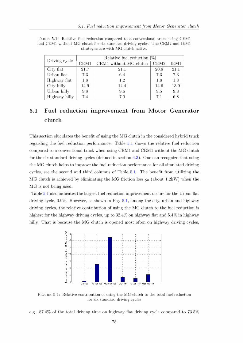
5.1. Fuel reduction improvement from Motor Generator clutch
Table 5.1: Relative fuel reduction compared to a conventional truck using CEM1and CEM1 without MG clutch for six standard driving cycles. The CEM2 and IEM1
strategies are with MG clutch active.
Driving cycleRelative fuel reduction [%]
CEM1 CEM1 without MG clutch CEM2 IEM1
City flat 21.7 21.1 20.8 21.1Urban flat 7.3 6.4 7.3 7.3Highway flat 1.8 1.2 1.8 1.8City hilly 14.9 14.4 14.6 13.9Urban hilly 9.8 9.6 9.5 9.8Highway hilly 7.4 7.0 7.1 6.8
5.1 Fuel reduction improvement from Motor Generator
clutch
This section elucidates the benefit of using the MG clutch in the considered hybrid truck
regarding the fuel reduction performance. Table 5.1 shows the relative fuel reduction
compared to a conventional truck when using CEM1 and CEM1 without the MG clutch
for the six standard driving cycles (defined in section 4.3). One can recognize that using
the MG clutch helps to improve the fuel reduction performance for all simulated driving
cycles, see the second and third columns of Table 5.1. The benefit from utilizing the
MG clutch is achieved by eliminating the MG friction loss g0 (about 1.2kW) when the
MG is not being used.
Table 5.1 also indicates the largest fuel reduction improvement occurs for the Urban flat
driving cycle, 0.9%. However, as shown in Fig. 5.1, among the city, urban and highway
driving cycles, the relative contribution of using the MG clutch to the fuel reduction is
highest for the highway driving cycles, up to 32.4% on highway flat and 5.4% in highway
hilly. That is because the MG clutch is opened most often on highway driving cycles,
Figure 5.1: Relative contribution of using the MG clutch to the total fuel reductionfor six standard driving cycles
e.g., 87.4% of the total driving time on highway flat driving cycle compared to 73.5%
78
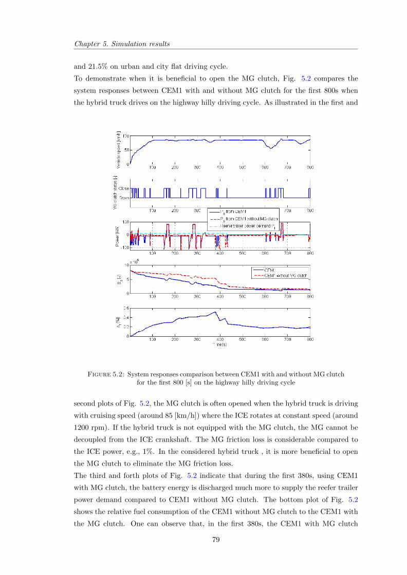
Chapter 5. Simulation results
and 21.5% on urban and city flat driving cycle.
To demonstrate when it is beneficial to open the MG clutch, Fig. 5.2 compares the
system responses between CEM1 with and without MG clutch for the first 800s when
the hybrid truck drives on the highway hilly driving cycle. As illustrated in the first and
Figure 5.2: System responses comparison between CEM1 with and without MG clutchfor the first 800 [s] on the highway hilly driving cycle
second plots of Fig. 5.2, the MG clutch is often opened when the hybrid truck is driving
with cruising speed (around 85 [km/h]) where the ICE rotates at constant speed (around
1200 rpm). If the hybrid truck is not equipped with the MG clutch, the MG cannot be
decoupled from the ICE crankshaft. The MG friction loss is considerable compared to
the ICE power, e.g., 1%. In the considered hybrid truck , it is more beneficial to open
the MG clutch to eliminate the MG friction loss.
The third and forth plots of Fig. 5.2 indicate that during the first 380s, using CEM1
with MG clutch, the battery energy is discharged much more to supply the reefer trailer
power demand compared to CEM1 without MG clutch. The bottom plot of Fig. 5.2
shows the relative fuel consumption of the CEM1 without MG clutch to the CEM1 with
the MG clutch. One can observe that, in the first 380s, the CEM1 with MG clutch
79

5.2. Integrated energy management strategy performance
consumes less fuel compared to the CEM1 without MG clutch (around 0.5%) while in
the period from 380s to 800s, CEM1 with MG clutch consumes more fuel, around 0.3%.
As a result, in the first 800s on the highway hilly driving cycle, the CEM1 with MG
clutch consumes less fuel, i.e., 0.2%, compared to without MG clutch.
5.2 Integrated energy management strategy performance
This section demonstrates how the IEM1 strategy manages the battery capacity loss ef-
fectively. The simulations encompass the six representative driving cycles. The driving
Figure 5.3: Normalized histogram of the hybrid truck operating modes for typicaldriving cycles with different settings of λo2. λo2 = 0, 250e3 and 500e3 are denoted
correspondingly in blue, green and red columns.
cycles’ characteristics are shown in Table 4.1. Fig. 5.3 shows the normalized number of
80
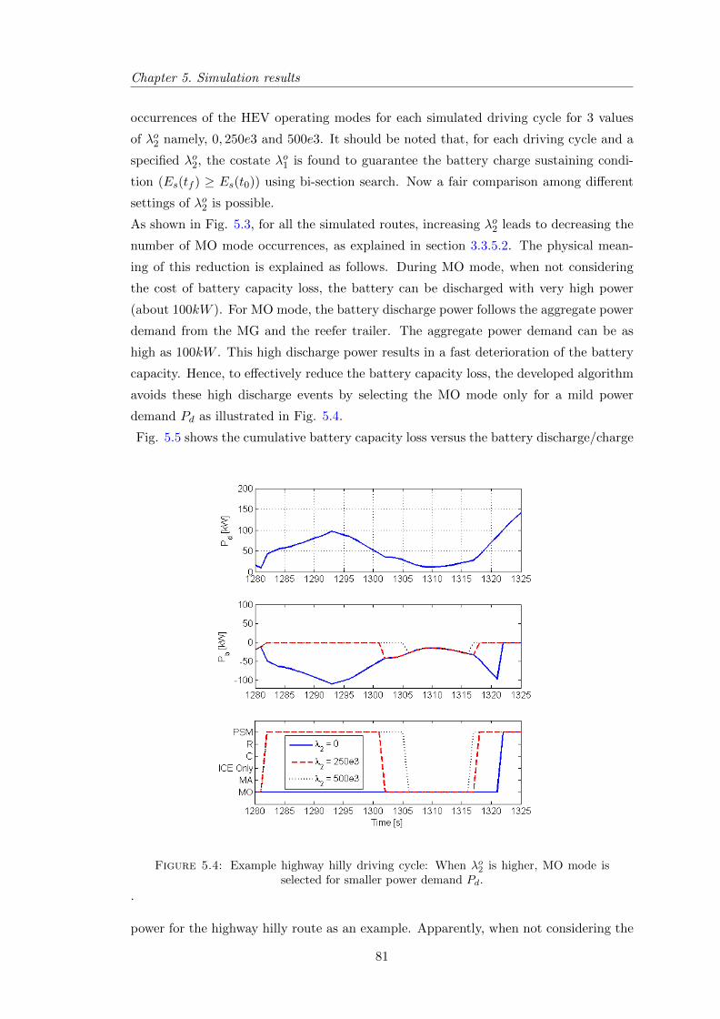
Chapter 5. Simulation results
occurrences of the HEV operating modes for each simulated driving cycle for 3 values
of λo2 namely, 0, 250e3 and 500e3. It should be noted that, for each driving cycle and a
specified λo2, the costate λo1 is found to guarantee the battery charge sustaining condi-
tion (Es(tf ) ≥ Es(t0)) using bi-section search. Now a fair comparison among different
settings of λo2 is possible.
As shown in Fig. 5.3, for all the simulated routes, increasing λo2 leads to decreasing the
number of MO mode occurrences, as explained in section 3.3.5.2. The physical mean-
ing of this reduction is explained as follows. During MO mode, when not considering
the cost of battery capacity loss, the battery can be discharged with very high power
(about 100kW ). For MO mode, the battery discharge power follows the aggregate power
demand from the MG and the reefer trailer. The aggregate power demand can be as
high as 100kW . This high discharge power results in a fast deterioration of the battery
capacity. Hence, to effectively reduce the battery capacity loss, the developed algorithm
avoids these high discharge events by selecting the MO mode only for a mild power
demand Pd as illustrated in Fig. 5.4.
Fig. 5.5 shows the cumulative battery capacity loss versus the battery discharge/charge
Figure 5.4: Example highway hilly driving cycle: When λo2 is higher, MO mode isselected for smaller power demand Pd.
.
power for the highway hilly route as an example. Apparently, when not considering the
81
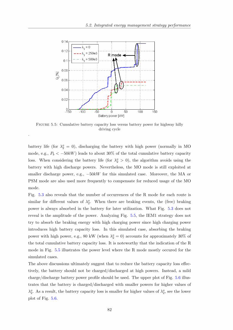
5.2. Integrated energy management strategy performance
Figure 5.5: Cumulative battery capacity loss versus battery power for highway hillydriving cycle
.
battery life (for λo2 = 0), discharging the battery with high power (normally in MO
mode, e.g., Pb < −50kW ) leads to about 30% of the total cumulative battery capacity
loss. When considering the battery life (for λo2 > 0), the algorithm avoids using the
battery with high discharge powers. Nevertheless, the MO mode is still exploited at
smaller discharge power, e.g., −50kW for this simulated case. Moreover, the MA or
PSM mode are also used more frequently to compensate for reduced usage of the MO
mode.
Fig. 5.3 also reveals that the number of occurrences of the R mode for each route is
similar for different values of λo2. When there are braking events, the (free) braking
power is always absorbed in the battery for later utilization. What Fig. 5.3 does not
reveal is the amplitude of the power. Analyzing Fig. 5.5, the IEM1 strategy does not
try to absorb the braking energy with high charging power since high charging power
introduces high battery capacity loss. In this simulated case, absorbing the braking
power with high power, e.g., 80 kW (when λo2 = 0) accounts for approximately 30% of
the total cumulative battery capacity loss. It is noteworthy that the indication of the R
mode in Fig. 5.5 illustrates the power level where the R mode mostly occured for the
simulated cases.
The above discussions ultimately suggest that to reduce the battery capacity loss effec-
tively, the battery should not be charged/discharged at high powers. Instead, a mild
charge/discharge battery power profile should be used. The upper plot of Fig. 5.6 illus-
trates that the battery is charged/discharged with smaller powers for higher values of
λo2. As a result, the battery capacity loss is smaller for higher values of λo2, see the lower
plot of Fig. 5.6.
82
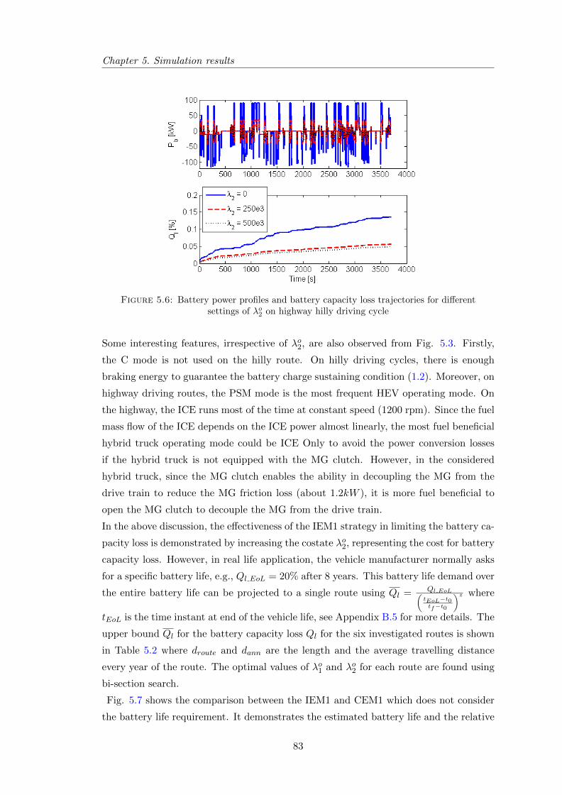
Chapter 5. Simulation results
Figure 5.6: Battery power profiles and battery capacity loss trajectories for differentsettings of λo2 on highway hilly driving cycle
Some interesting features, irrespective of λo2, are also observed from Fig. 5.3. Firstly,
the C mode is not used on the hilly route. On hilly driving cycles, there is enough
braking energy to guarantee the battery charge sustaining condition (1.2). Moreover, on
highway driving routes, the PSM mode is the most frequent HEV operating mode. On
the highway, the ICE runs most of the time at constant speed (1200 rpm). Since the fuel
mass flow of the ICE depends on the ICE power almost linearly, the most fuel beneficial
hybrid truck operating mode could be ICE Only to avoid the power conversion losses
if the hybrid truck is not equipped with the MG clutch. However, in the considered
hybrid truck, since the MG clutch enables the ability in decoupling the MG from the
drive train to reduce the MG friction loss (about 1.2kW ), it is more fuel beneficial to
open the MG clutch to decouple the MG from the drive train.
In the above discussion, the effectiveness of the IEM1 strategy in limiting the battery ca-
pacity loss is demonstrated by increasing the costate λo2, representing the cost for battery
capacity loss. However, in real life application, the vehicle manufacturer normally asks
for a specific battery life, e.g., Ql EoL = 20% after 8 years. This battery life demand over
the entire battery life can be projected to a single route using Ql = Ql EoL(tEoL−t0tf−t0
)z where
tEoL is the time instant at end of the vehicle life, see Appendix B.5 for more details. The
upper bound Ql for the battery capacity loss Ql for the six investigated routes is shown
in Table 5.2 where droute and dann are the length and the average travelling distance
every year of the route. The optimal values of λo1 and λo2 for each route are found using
bi-section search.
Fig. 5.7 shows the comparison between the IEM1 and CEM1 which does not consider
the battery life requirement. It demonstrates the estimated battery life and the relative
83
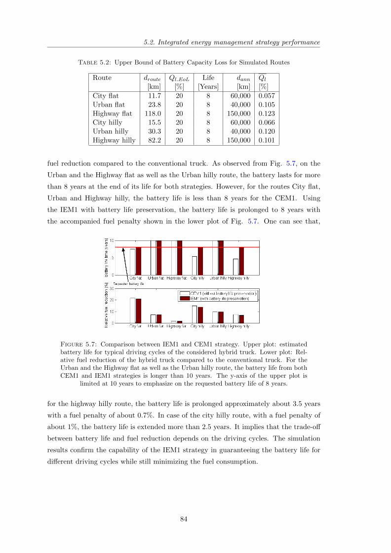
5.2. Integrated energy management strategy performance
Table 5.2: Upper Bound of Battery Capacity Loss for Simulated Routes
Route droute Ql EoL Life dann Ql[km] [%] [Years] [km] [%]
City flat 11.7 20 8 60,000 0.057Urban flat 23.8 20 8 40,000 0.105Highway flat 118.0 20 8 150,000 0.123City hilly 15.5 20 8 60,000 0.066Urban hilly 30.3 20 8 40,000 0.120Highway hilly 82.2 20 8 150,000 0.101
fuel reduction compared to the conventional truck. As observed from Fig. 5.7, on the
Urban and the Highway flat as well as the Urban hilly route, the battery lasts for more
than 8 years at the end of its life for both strategies. However, for the routes City flat,
Urban and Highway hilly, the battery life is less than 8 years for the CEM1. Using
the IEM1 with battery life preservation, the battery life is prolonged to 8 years with
the accompanied fuel penalty shown in the lower plot of Fig. 5.7. One can see that,
Figure 5.7: Comparison between IEM1 and CEM1 strategy. Upper plot: estimatedbattery life for typical driving cycles of the considered hybrid truck. Lower plot: Rel-ative fuel reduction of the hybrid truck compared to the conventional truck. For theUrban and the Highway flat as well as the Urban hilly route, the battery life from bothCEM1 and IEM1 strategies is longer than 10 years. The y-axis of the upper plot is
limited at 10 years to emphasize on the requested battery life of 8 years.
for the highway hilly route, the battery life is prolonged approximately about 3.5 years
with a fuel penalty of about 0.7%. In case of the city hilly route, with a fuel penalty of
about 1%, the battery life is extended more than 2.5 years. It implies that the trade-off
between battery life and fuel reduction depends on the driving cycles. The simulation
results confirm the capability of the IEM1 strategy in guaranteeing the battery life for
different driving cycles while still minimizing the fuel consumption.
84
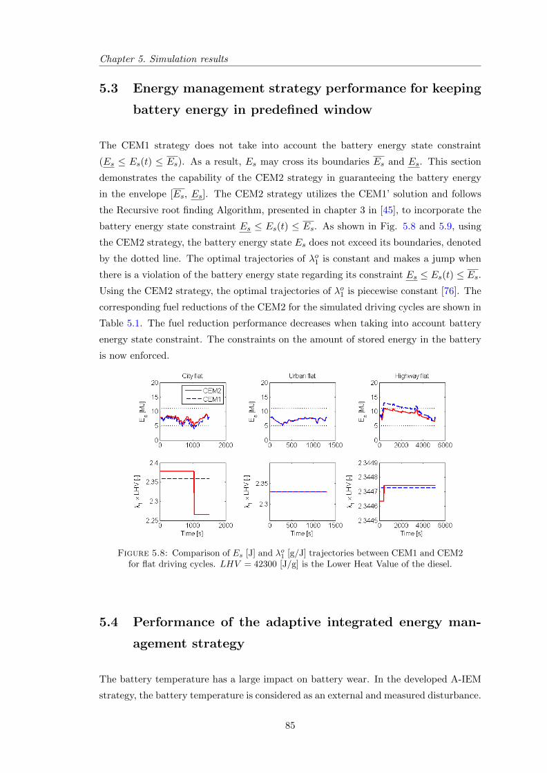
Chapter 5. Simulation results
5.3 Energy management strategy performance for keeping
battery energy in predefined window
The CEM1 strategy does not take into account the battery energy state constraint
(Es ≤ Es(t) ≤ Es). As a result, Es may cross its boundaries Es and Es. This section
demonstrates the capability of the CEM2 strategy in guaranteeing the battery energy
in the envelope [Es, Es]. The CEM2 strategy utilizes the CEM1’ solution and follows
the Recursive root finding Algorithm, presented in chapter 3 in [45], to incorporate the
battery energy state constraint Es ≤ Es(t) ≤ Es. As shown in Fig. 5.8 and 5.9, using
the CEM2 strategy, the battery energy state Es does not exceed its boundaries, denoted
by the dotted line. The optimal trajectories of λo1 is constant and makes a jump when
there is a violation of the battery energy state regarding its constraint Es ≤ Es(t) ≤ Es.Using the CEM2 strategy, the optimal trajectories of λo1 is piecewise constant [76]. The
corresponding fuel reductions of the CEM2 for the simulated driving cycles are shown in
Table 5.1. The fuel reduction performance decreases when taking into account battery
energy state constraint. The constraints on the amount of stored energy in the battery
is now enforced.
Figure 5.8: Comparison of Es [J] and λo1 [g/J] trajectories between CEM1 and CEM2for flat driving cycles. LHV = 42300 [J/g] is the Lower Heat Value of the diesel.
5.4 Performance of the adaptive integrated energy man-
agement strategy
The battery temperature has a large impact on battery wear. In the developed A-IEM
strategy, the battery temperature is considered as an external and measured disturbance.
85
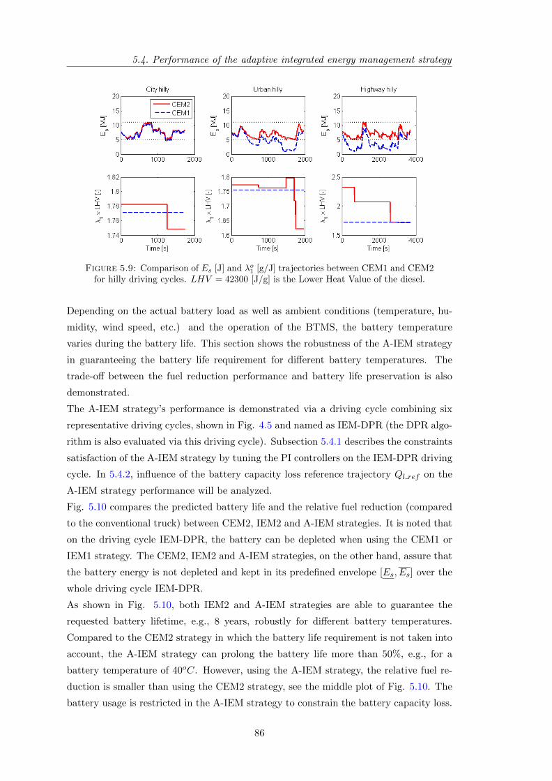
5.4. Performance of the adaptive integrated energy management strategy
Figure 5.9: Comparison of Es [J] and λo1 [g/J] trajectories between CEM1 and CEM2for hilly driving cycles. LHV = 42300 [J/g] is the Lower Heat Value of the diesel.
Depending on the actual battery load as well as ambient conditions (temperature, hu-
midity, wind speed, etc.) and the operation of the BTMS, the battery temperature
varies during the battery life. This section shows the robustness of the A-IEM strategy
in guaranteeing the battery life requirement for different battery temperatures. The
trade-off between the fuel reduction performance and battery life preservation is also
demonstrated.
The A-IEM strategy’s performance is demonstrated via a driving cycle combining six
representative driving cycles, shown in Fig. 4.5 and named as IEM-DPR (the DPR algo-
rithm is also evaluated via this driving cycle). Subsection 5.4.1 describes the constraints
satisfaction of the A-IEM strategy by tuning the PI controllers on the IEM-DPR driving
cycle. In 5.4.2, influence of the battery capacity loss reference trajectory Ql ref on the
A-IEM strategy performance will be analyzed.
Fig. 5.10 compares the predicted battery life and the relative fuel reduction (compared
to the conventional truck) between CEM2, IEM2 and A-IEM strategies. It is noted that
on the driving cycle IEM-DPR, the battery can be depleted when using the CEM1 or
IEM1 strategy. The CEM2, IEM2 and A-IEM strategies, on the other hand, assure that
the battery energy is not depleted and kept in its predefined envelope [Es, Es] over the
whole driving cycle IEM-DPR.
As shown in Fig. 5.10, both IEM2 and A-IEM strategies are able to guarantee the
requested battery lifetime, e.g., 8 years, robustly for different battery temperatures.
Compared to the CEM2 strategy in which the battery life requirement is not taken into
account, the A-IEM strategy can prolong the battery life more than 50%, e.g., for a
battery temperature of 40oC. However, using the A-IEM strategy, the relative fuel re-
duction is smaller than using the CEM2 strategy, see the middle plot of Fig. 5.10. The
battery usage is restricted in the A-IEM strategy to constrain the battery capacity loss.
86
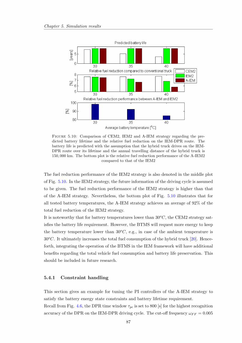
Chapter 5. Simulation results
Figure 5.10: Comparison of CEM2, IEM2 and A-IEM strategy regarding the pre-dicted battery lifetime and the relative fuel reduction on the IEM-DPR route. Thebattery life is predicted with the assumption that the hybrid truck drives on the IEM-DPR route over its lifetime and the annual travelling distance of the hybrid truck is150, 000 km. The bottom plot is the relative fuel reduction performance of the A-IEM2
compared to that of the IEM2
The fuel reduction performance of the IEM2 strategy is also denoted in the middle plot
of Fig. 5.10. In the IEM2 strategy, the future information of the driving cycle is assumed
to be given. The fuel reduction performance of the IEM2 strategy is higher than that
of the A-IEM strategy. Nevertheless, the bottom plot of Fig. 5.10 illustrates that for
all tested battery temperatures, the A-IEM strategy achieves an average of 92% of the
total fuel reduction of the IEM2 strategy.
It is noteworthy that for battery temperatures lower than 30oC, the CEM2 strategy sat-
isfies the battery life requirement. However, the BTMS will request more energy to keep
the battery temperature lower than 30oC, e.g., in case of the ambient temperature is
30oC. It ultimately increases the total fuel consumption of the hybrid truck [20]. Hence-
forth, integrating the operation of the BTMS in the IEM framework will have additional
benefits regarding the total vehicle fuel consumption and battery life preservation. This
should be included in future research.
5.4.1 Constraint handling
This section gives an example for tuning the PI controllers of the A-IEM strategy to
satisfy the battery energy state constraints and battery lifetime requirement.
Recall from Fig. 4.6, the DPR time window τpc is set to 800 [s] for the highest recognition
accuracy of the DPR on the IEM-DPR driving cycle. The cut-off frequency ωFF = 0.005
87
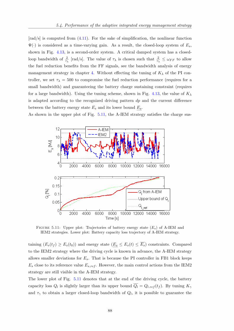
5.4. Performance of the adaptive integrated energy management strategy
[rad/s] is computed from (4.11). For the sake of simplification, the nonlinear function
Ψ(·) is considered as a time-varying gain. As a result, the closed-loop system of Es,
shown in Fig. 4.13, is a second-order system. A critical damped system has a closed-
loop bandwidth of 2τλ
[rad/s]. The value of τλ is chosen such that 2τλ≤ ωFF to allow
the fuel reduction benefits from the FF signals, see the bandwidth analysis of energy
management strategy in chapter 4. Without effecting the tuning of Kλ of the PI con-
troller, we set τλ = 500 to compromise the fuel reduction performance (requires for a
small bandwidth) and guaranteeing the battery charge sustaining constraint (requires
for a large bandwidth). Using the tuning scheme, shown in Fig. 4.13, the value of Kλ
is adapted according to the recognized driving pattern dp and the current difference
between the battery energy state Es and its lower bound Es.
As shown in the upper plot of Fig. 5.11, the A-IEM strategy satisfies the charge sus-
Figure 5.11: Upper plot: Trajectories of battery energy state (Es) of A-IEM andIEM2 strategies. Lower plot: Battery capacity loss trajectory of A-IEM strategy.
taining (Es(tf ) ≥ Es(t0)) and energy state (Es ≤ Es(t) ≤ Es) constraints. Compared
to the IEM2 strategy where the driving cycle is known in advance, the A-IEM strategy
allows smaller deviations for Es. That is because the PI controller in FB1 block keeps
Es close to its reference value Es ref . However, the main control actions from the IEM2
strategy are still visible in the A-IEM strategy.
The lower plot of Fig. 5.11 denotes that at the end of the driving cycle, the battery
capacity loss Ql is slightly larger than its upper bound Ql = Ql ref (tf ). By tuning Kγ
and τγ to obtain a larger closed-loop bandwidth of Ql, it is possible to guarantee the
88
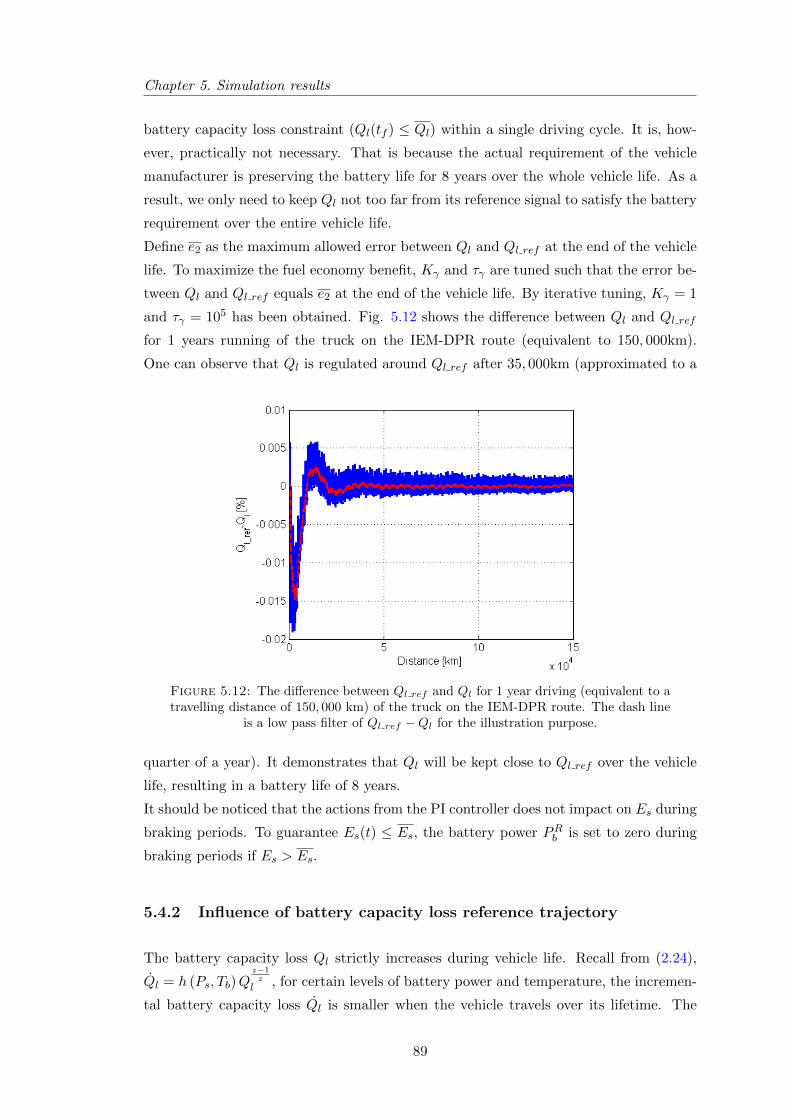
Chapter 5. Simulation results
battery capacity loss constraint (Ql(tf ) ≤ Ql) within a single driving cycle. It is, how-
ever, practically not necessary. That is because the actual requirement of the vehicle
manufacturer is preserving the battery life for 8 years over the whole vehicle life. As a
result, we only need to keep Ql not too far from its reference signal to satisfy the battery
requirement over the entire vehicle life.
Define e2 as the maximum allowed error between Ql and Ql ref at the end of the vehicle
life. To maximize the fuel economy benefit, Kγ and τγ are tuned such that the error be-
tween Ql and Ql ref equals e2 at the end of the vehicle life. By iterative tuning, Kγ = 1
and τγ = 105 has been obtained. Fig. 5.12 shows the difference between Ql and Ql ref
for 1 years running of the truck on the IEM-DPR route (equivalent to 150, 000km).
One can observe that Ql is regulated around Ql ref after 35, 000km (approximated to a
Figure 5.12: The difference between Ql ref and Ql for 1 year driving (equivalent to atravelling distance of 150, 000 km) of the truck on the IEM-DPR route. The dash line
is a low pass filter of Ql ref −Ql for the illustration purpose.
quarter of a year). It demonstrates that Ql will be kept close to Ql ref over the vehicle
life, resulting in a battery life of 8 years.
It should be noticed that the actions from the PI controller does not impact on Es during
braking periods. To guarantee Es(t) ≤ Es, the battery power PRb is set to zero during
braking periods if Es > Es.
5.4.2 Influence of battery capacity loss reference trajectory
The battery capacity loss Ql strictly increases during vehicle life. Recall from (2.24),
Ql = h (Ps, Tb)Qz−1z
l , for certain levels of battery power and temperature, the incremen-
tal battery capacity loss Ql is smaller when the vehicle travels over its lifetime. The
89
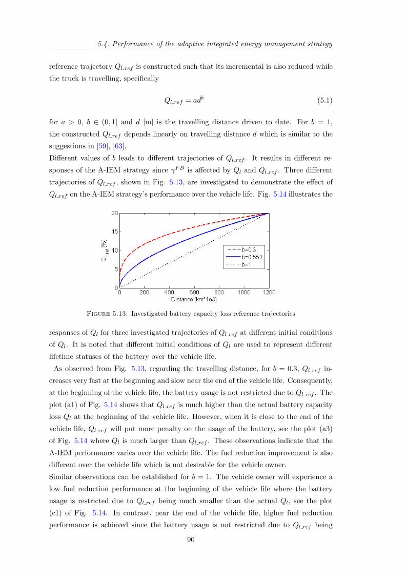
5.4. Performance of the adaptive integrated energy management strategy
reference trajectory Ql ref is constructed such that its incremental is also reduced while
the truck is travelling, specifically
Ql ref = adb (5.1)
for a > 0, b ∈ (0, 1] and d [m] is the travelling distance driven to date. For b = 1,
the constructed Ql ref depends linearly on travelling distance d which is similar to the
suggestions in [59], [63].
Different values of b leads to different trajectories of Ql ref . It results in different re-
sponses of the A-IEM strategy since γFB is affected by Ql and Ql ref . Three different
trajectories of Ql ref , shown in Fig. 5.13, are investigated to demonstrate the effect of
Ql ref on the A-IEM strategy’s performance over the vehicle life. Fig. 5.14 illustrates the
Figure 5.13: Investigated battery capacity loss reference trajectories
responses of Ql for three investigated trajectories of Ql ref at different initial conditions
of Ql. It is noted that different initial conditions of Ql are used to represent different
lifetime statuses of the battery over the vehicle life.
As observed from Fig. 5.13, regarding the travelling distance, for b = 0.3, Ql ref in-
creases very fast at the beginning and slow near the end of the vehicle life. Consequently,
at the beginning of the vehicle life, the battery usage is not restricted due to Ql ref . The
plot (a1) of Fig. 5.14 shows that Ql ref is much higher than the actual battery capacity
loss Ql at the beginning of the vehicle life. However, when it is close to the end of the
vehicle life, Ql ref will put more penalty on the usage of the battery, see the plot (a3)
of Fig. 5.14 where Ql is much larger than Ql ref . These observations indicate that the
A-IEM performance varies over the vehicle life. The fuel reduction improvement is also
different over the vehicle life which is not desirable for the vehicle owner.
Similar observations can be established for b = 1. The vehicle owner will experience a
low fuel reduction performance at the beginning of the vehicle life where the battery
usage is restricted due to Ql ref being much smaller than the actual Ql, see the plot
(c1) of Fig. 5.14. In contrast, near the end of the vehicle life, higher fuel reduction
performance is achieved since the battery usage is not restricted due to Ql ref being
90
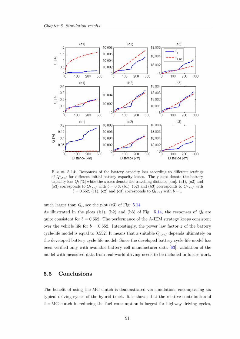
Chapter 5. Simulation results
Figure 5.14: Responses of the battery capacity loss according to different settingsof Ql ref for different initial battery capacity losses. The y axes denote the batterycapacity loss Ql [%] while the x axes denote the travelling distance [km]. (a1), (a2) and(a3) corresponds to Ql ref with b = 0.3; (b1), (b2) and (b3) corresponds to Ql ref with
b = 0.552; (c1), (c2) and (c3) corresponds to Ql ref with b = 1
much larger than Ql, see the plot (c3) of Fig. 5.14.
As illustrated in the plots (b1), (b2) and (b3) of Fig. 5.14, the responses of Ql are
quite consistent for b = 0.552. The performance of the A-IEM strategy keeps consistent
over the vehicle life for b = 0.552. Interestingly, the power law factor z of the battery
cycle-life model is equal to 0.552. It means that a suitable Ql ref depends ultimately on
the developed battery cycle-life model. Since the developed battery cycle-life model has
been verified only with available battery cell manufacturer data [63], validation of the
model with measured data from real-world driving needs to be included in future work.
5.5 Conclusions
The benefit of using the MG clutch is demonstrated via simulations encompassing six
typical driving cycles of the hybrid truck. It is shown that the relative contribution of
the MG clutch in reducing the fuel consumption is largest for highway driving cycles,
91
5.5. Conclusions
about 32.4%, where the MG clutch is opened most often.
Simulation results verify the analytical analysis that the IEM1 strategy preserves the
battery life effectively by avoid charging/discharging the battery at too high powers.
Nevertheless, the fuel consumption is still reduced by utilizing the battery at a mild
battery power profile. Although the trade-off between fuel reduction and battery life
depends on the driving cycle, simulation results show that the IEM1 strategy guarantees
the battery life requirement for different driving scenarios.
Simulation results also demonstrate that the A-IEM strategy is able to guarantee ro-
bustly the battery life requirement for different driving scenarios without knowing the
future information of the driving cycle. On average, the fuel reduction performance of
the A-IEM strategy attains around 92% that of the IEM2 strategy requiring the full
knowledge of the driving cycle.
92
Chapter 6
Conclusions and
recommendations
This chapter summarizes the main conclusions of this thesis in section 6.1. Recommen-
dations for future research arising from this research are given in section 6.2.
6.1 Conclusions
This thesis studied a parallel hybrid electric heavy-duty truck. The considered hybrid
truck is equipped with a clutch system to support decoupling of both the ICE and MG
from the drive train to drive electrically and/or eliminate their drag losses. Regarding
the research objectives presented in chapter 1, the following conclusions are made:
• Energy Management Strategies (EMSs) CEM1 and CEM2, which focus on fuel
consumption and not on battery lifetime, are developed to minimize the hybrid
truck fuel consumption while keeping the stored battery energy (Es) in a predefined
operating range. With the assumption that future information of the driving cycle
is known, analytical solutions to the CEM1 and CEM2 strategies are derived to
optimize the battery charge/dicharge power and the operation of the clutch system.
• When taking into account the battery life requirement, the developed EMSs are ex-
tended to the Integrated Energy Management Strategies (IEM), IEM1 and IEM2.
The IEM1 and IEM2 strategies minimize the hybrid truck fuel consumption within
the battery life requirement. Solutions for the IEM1 and IEM2 strategies are
also derived analytically to optimize the clutch system operation and battery
charge/discharge power. Knowledge of the future driving cycle information is
93
6.1. Conclusions
needed to achieve the optimal analytical solutions of the IEM1 and IEM2 strate-
gies.
• In chapter 4, without requesting knowledge of the future driving cycle, a real-
time implementation of the Adaptive Integrated Energy Management (A-IEM)
strategy is developed to satisfy the battery life requirement and to achieve a fuel
reduction performance close to that of the IEM2 strategy. For all the simulated
driving scenarios, the A-IEM strategy achieves an average of 92% of the total fuel
reduction of the IEM2 strategy.
In [44], the author shows that the EMS utilizes three characteristics for reducing the
vehicle fuel consumption namely, the slope of the ICE fuel map, the ICE drag loss
and the regeneration of free kinetic energy during braking periods. Besides
these characteristics, this thesis, analyzing the analytical solutions and simulation re-
sults, identifies additional characteristics for fuel reduction and battery life preservation:
• The Motor Generator (MG) friction loss as function of MG speed can be
eliminated by opening the MG clutch and turning off the MG. When the MG is
connected to the drive train but electrically inactive, it produces no mechanical/-
electric power but it still requests power to counteract its friction loss. When the
MG clutch is open, this friction loss can be eliminated by turning off the MG. The
hybrid truck is now propelled by the ICE and the reefer trailer is supplied by the
battery. This thesis shows that the power conversion loss and the friction loss in
the MG, compared to the battery power loss, determine when it is profitable to
open the MG clutch and turn off the MG.
• To preserve the battery life, the battery should not be charged/discharged
at too high power to avoid high deterioration of its capacity. However, restrict-
ing the battery usage results in a penalty on the total fuel consumption of the
hybrid truck. This thesis shows that there exists a compromise between battery
life preservation and fuel reduction performance of the hybrid truck. For exam-
ple, when not considering the battery wear, regenerative braking energy is always
profitable to be absorbed in the battery. When the battery wear is taken into
account, maximum regenerative braking is not always beneficial. High
charging powers during the braking periods should be avoided to prevent too fast
deterioration of the battery capacity. This thesis proposed such an upper bound
for braking power.
The battery life is preserved in the A-IEM strategy by
94
Chapter 6. Conclusions and recommendations
• Artificially increasing the battery power loss in the Hamiltonian func-
tion using an adaptive factor γ when necessary. It restricts the battery usage to
reduce its wear.
The fuel reduction performance of the A-IEM strategy is achieved by
• Appropriate estimation of the A-IEM control parameters (costate λ1 and
the adaptive factor γ) for each specific driving pattern in the driving cycle. A
Driving Pattern Recognition algorithm, utilizing the Principal Component Analy-
sis technique, is used to recognize the current driving pattern. The optimal values
of λ1 and γ are computed off-line and stored in a look-up table for a number of
standard driving patterns.
• A correct tuning of the PI controllers in the battery energy Es and battery ca-
pacity loss Ql loops leads to appropriate closed-loop bandwidths for both
Es and Ql: It prevents Es and Ql to drift away from their reference trajectories
due to the inaccuracy in recognizing the driving pattern. Besides, it still allows
enough freedom for storing/retrieving energy into/from the battery to obtain fuel
reduction benefits.
6.2 Recommendations
This thesis has developed both the off-line and on-line energy management strategies to
minimize the fuel consumption of the hybrid truck with (equipped with the ICE and MG
clutches) taking the battery life requirement explicitly into account. Some extensions
from this research are suggested:
• The battery cycle-life has a large impact on the system performance. The bat-
tery cycle-life is currently verified with only the battery manufacturer data with
standard charge/dicharge cycle and temperature. A validation of the developed
battery cycle-life model with real-life driving data is foreseen as future research.
• The developed A-IEM strategy utilizes only the past information from the driving
cycle to estimate the control parameters. Owing to the availability of the preview
information from a GPS or ITS system, the A-IEM can be extended to capture
additional benefits from the preview information, e.g., a (feedforward-oriented)
correction of DPR block.
• Integrating the battery temperature dynamics and the Battery Thermal Man-
agement System operation into the IEM framework is shown to be feasible with a
95
6.2. Recommendations 96
numerical solution. Verification of the numerical solution via simulation and deriv-
ing an analytical solution to the new Integrated Energy and Thermal Management
(IETM) strategy are relevant future research topics. They will bring more insight
into the cost balancing among the fuel consumption, battery heating/cooling op-
eration and the battery wear.
• Combination of battery and supercapacitor: When taking the battery wear into
account, the battery is not charged/discharged at peak powers to prevent the
battery from its high capacity loss region, see Fig. 2.12. Consequently, when
considering the battery wear in the EMS, the fuel reduction (compared to a con-
ventional truck) will be less than that when not considering battery wear in the
EMS. To avoid this loss, the battery can be used in combination with a superca-
pacitor. The supercapacitor features a much higher power density, a longer life
cycle with high efficiency and fast charging/discharging responses [85]. Hence, it
is well suited for charging/discharging with peak powers. Although a small energy
density is the main disadvantage of the supercapacitor, combining the battery and
supercapacitor may preserve the battery life without losing any potential fuel ben-
efit from the hybrid powertrain. Extending the developed strategies to handle also
the supercapacitor operation will influence the presented results and yields some
challenges in control algorithms.
• In the considered hybrid truck, by opening the ICE and/or MG clutches, the ICE
and/or MG are decoupled from the drive train. As a result, the ICE and/or
MG can be turned off to eliminate their drag losses to improve the fuel reduction
performance of the hybrid truck. So far, the ICE and MG starts/stops are not
penalized by the CEM1, CEM2, IEM1, IEM2 and A-IEM strategies. They will be
important issues when the driveability is respect. Moreover, frequent starts/stops
of the ICE and MG request frequent opening/closing the ICE and MG clutches
which are not desirable for the ICE and MG clutches’ durability. To incorporate
the penalties on ICE and MG start/stop, a valid approach is to include extra en-
ergy losses for starting the ICE and MG in their models. This method is proposed
to make a trade-off between the cost (from driveability, clutches’ durability) and
profits (from the fuel reduction) when utilizing the ICE and MG start/stop func-
tionality. A start has been made in [86] where an ICE start loss model is utilized
to investigate the effects of ICE start losses on EMSs and fuel consumption for a
parallel hybrid electric vehicle.
96
Appendix A
Mathematical derivation of
energy management without
battery life preservation
A.1 Optimal battery power in MA and C mode for CEM1
Regarding minPb∈[Pb,0)
HMA, the battery power Pb which minimize HMA is obtained by
solving the equation
∂HMA
∂Pb= 0 (A.1)
α1η−e − λo1 (1− 2βPb) = 0 (A.2)
for Pb ∈[Pb, 0
). As a result, the optimal battery power in the MA mode is achieved as
P ob = PMAb = min
(max
(Pb,
λo1 − α1η−e
2λo1β
), 0
)(A.3)
In terms of minPb∈(0,Pb]
HC , the battery power Pb minimizing HC is computed from solving
the equation
∂HC
∂Pb= 0 (A.4)
α1
η+e− λo1 (1− 2βPb) = 0 (A.5)
97
A.2. Hamiltonian function minimization for CEM1 98
for Pb ∈(0, Pb
]. Subsequently, the optimal battery power in the C mode is derived as
P ob = PCb = max
(min
(Pb,
λo1 − α1
η+e
2λo1β
), 0
)(A.6)
A.2 Hamiltonian function minimization for CEM1
It is obvious that the solution of (A.2) Pb =λo1−α1η
−e
2λo1βis smaller than 0 ∀0 < λo1 < α1η
−e
and the solution of (A.5) Pb =λo1−
α1
η+e2λo1β
is larger than 0 ∀λo1 > α1
η+e. Owing to these
observations, the Hamiltonian function H is analyzed for three intervals of λo1 namely,
(0, α1η−e ), [α1η
−e ,
α1
η+e],(α1
η+e,+∞
).
1. For 0 < λo1 < α1η−e : In this interval, the first derivative of HC with respect to Pb
satisfies ∂HC∂Pb
> 0, ∀Pb > 0. Therefore HC > limPb→0+
HC = HICEonly. Moreover,
since PMAb < 0, we have Ho
MA < limPb→0−
HMA = HICEonly. It follows that
HoMA < HICEonly < HC for 0 < λo1 < α1η
−e andPd > 0 (A.7)
2. For α1η−e ≤ λo1 ≤ α1
η+e: In this interval, we have ∂HMA
∂Pb< 0, ∀Pb < 0 and ∂HC
∂Pb>
0, ∀Pb > 0. Hence,
HC > limPb→0+
HC = HICEonly (A.8)
HMA > limPb→0−
HMA = HICEonly (A.9)
for all λ1 ∈[α1η
−e ,
α1
η+e
]and Pd > 0.
3. For λo1 >α1
η+e: In this interval, the first derivative of HMA with respect to Pb satisfies
∂HMA∂Pb
< 0, ∀Pb < 0. Therefore, HMA > limPb→0−
HMA = HICEonly. Moreover, since
PCb > 0 for λ1 >α1
η+e, we have Ho
C < limPb→0−
HC = HICEonly. It follows that
HoC < HICEonly < HMA for λ1 >
α1
η+eandPd > 0 (A.10)
Moreover, by solving (3.11)-(3.17), it is straight forward to obtain the following
properties: HoMA ≥ HMO for 0 < Pd ≤ PMA
dlim
HoMA ≥ HPSM forg0 ≥ gMA
0
(A.11)
98
Appendix A. Mathematical derivation of energy management without battery lifepreservation 99
Table A.1: Explicit expression of the power thresholds [W] used in determining theoptimal feasible HEV operating mode for CEM1.
Parameter Expression
PMAdlim
η−e [(λo1−α1η−e )−2√α2λo1β]
−2λo1β− Plη−e − g0
P ICEonlydlim
η−e
[(λo1−α1η
−e )−
√(λo1−α1η
−e )
2+4
(α2+α1Pl
(1
η+e−η−e
))λo1β
]−2λo1β
− Plη−e − g0
PCdlim
η−e
(λo1−α1η−e )−
√(λo1−α1η
−e )
2−(λo1−
α1
η+e
)2
+4
(α2+α1Pl
(1
η+e−η−e
))λo1β
−2λo1β
−Plη−e − g0
PPSMdlim
η−e
[(λo1−α1η
−e )−
√(λo1−α1η
−e )
2+4(λo1βP 2
l +(λo1−α1η−e )Pl+α2−α1g0)λo1β
]−2λo1β
−Plη−e − g0
gMA0
λo1(Pl+βP 2l )
α1+
(λo1−α1η−e )
2
4λo1βα1− Plη−e
gICEonly0
λo1(Pl+βP 2l )
α1− Pl
η+e
gC0λo1(Pl+βP 2
l )α1
+
(λo1−
α1
η+e
)2
4λo1βα1− Pl
η+e
HICEonly ≥ HMO for 0 < Pd ≤ P ICEonlydlim
HICEonly ≥ HPSM forg0 ≥ gICEonly0
(A.12)
HoC ≥ HMO for 0 < Pd ≤ PCdlim
HoC ≥ HPSM forg0 ≥ gC0
(A.13)
HPSM ≥ HMO for 0 < Pd ≤ PPSMdlim (A.14)
From (A.7), (A.8), (A.9), and (A.10)-(A.14), the solution shown in Table 3.2 is achieved.
It is noteworthy that for the equality of (A.11)-(A.14), e.g., Pd = P(.)dlim and g0 = g
(.)0 ,
the Hamiltonian function has two identical minima. Without loss of optimality, the MO
mode is chosen for Pd = P(.)dlim (see [43] for a similar observation) while the PSM mode
is chosen for g0 = g(.)0 and Pd > P
(.)dlim. The explicit expressions of the power thresholds
PMAdlim, P ICEonlydlim , PCdlim, PPSMdlim , gMA
0 , gICEonly0 and gC0 are given in Table A.1.
A.3 Influence of battery power loss coefficient on CEM1
As shown in Table 3.1, PMAb and PCb depend explicitly on λo1, β, α1 and η−e . Moreover, it
can be seen that changing the value of β only effects the size of PMAb and PCb . Increasing
β leads to a decrease of PMAb and PCb . In addition, PRb will be also reduced with higher
99
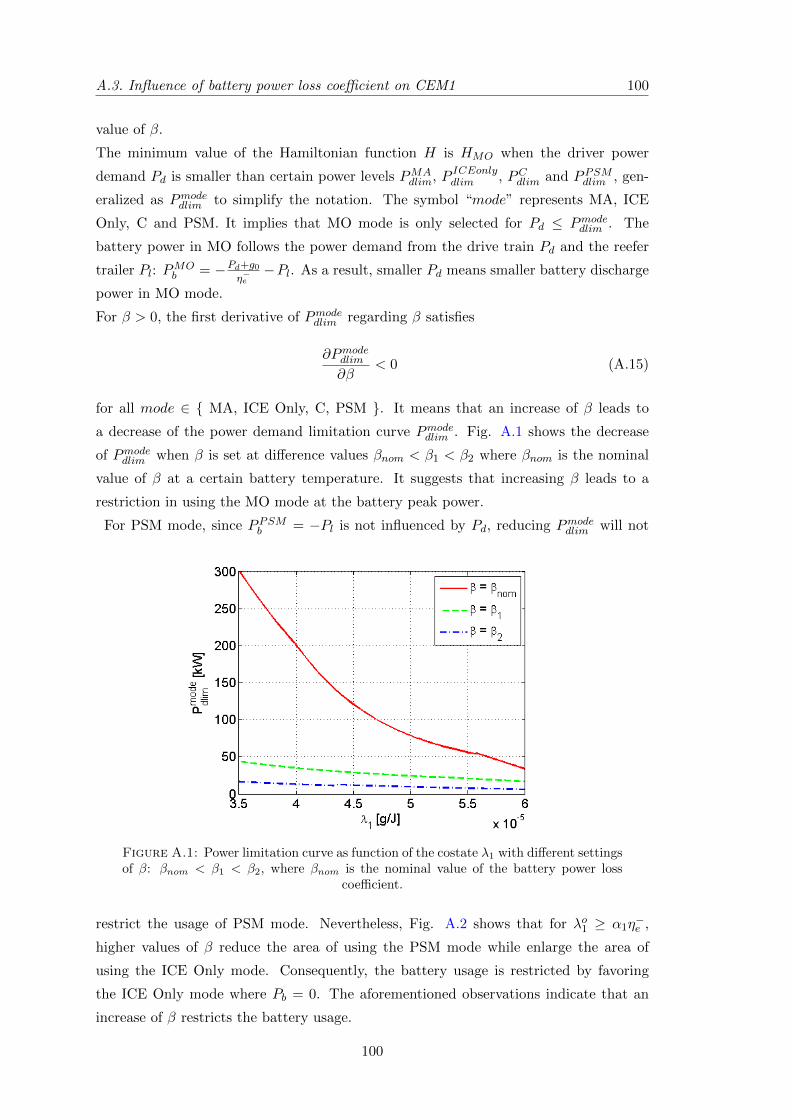
A.3. Influence of battery power loss coefficient on CEM1 100
value of β.
The minimum value of the Hamiltonian function H is HMO when the driver power
demand Pd is smaller than certain power levels PMAdlim, P ICEonlydlim , PCdlim and PPSMdlim , gen-
eralized as Pmodedlim to simplify the notation. The symbol “mode” represents MA, ICE
Only, C and PSM. It implies that MO mode is only selected for Pd ≤ Pmodedlim . The
battery power in MO follows the power demand from the drive train Pd and the reefer
trailer Pl: PMOb = −Pd+g0
η−e−Pl. As a result, smaller Pd means smaller battery discharge
power in MO mode.
For β > 0, the first derivative of Pmodedlim regarding β satisfies
∂Pmodedlim
∂β< 0 (A.15)
for all mode ∈ MA, ICE Only, C, PSM . It means that an increase of β leads to
a decrease of the power demand limitation curve Pmodedlim . Fig. A.1 shows the decrease
of Pmodedlim when β is set at difference values βnom < β1 < β2 where βnom is the nominal
value of β at a certain battery temperature. It suggests that increasing β leads to a
restriction in using the MO mode at the battery peak power.
For PSM mode, since PPSMb = −Pl is not influenced by Pd, reducing Pmodedlim will not
Figure A.1: Power limitation curve as function of the costate λ1 with different settingsof β: βnom < β1 < β2, where βnom is the nominal value of the battery power loss
coefficient.
restrict the usage of PSM mode. Nevertheless, Fig. A.2 shows that for λo1 ≥ α1η−e ,
higher values of β reduce the area of using the PSM mode while enlarge the area of
using the ICE Only mode. Consequently, the battery usage is restricted by favoring
the ICE Only mode where Pb = 0. The aforementioned observations indicate that an
increase of β restricts the battery usage.
100
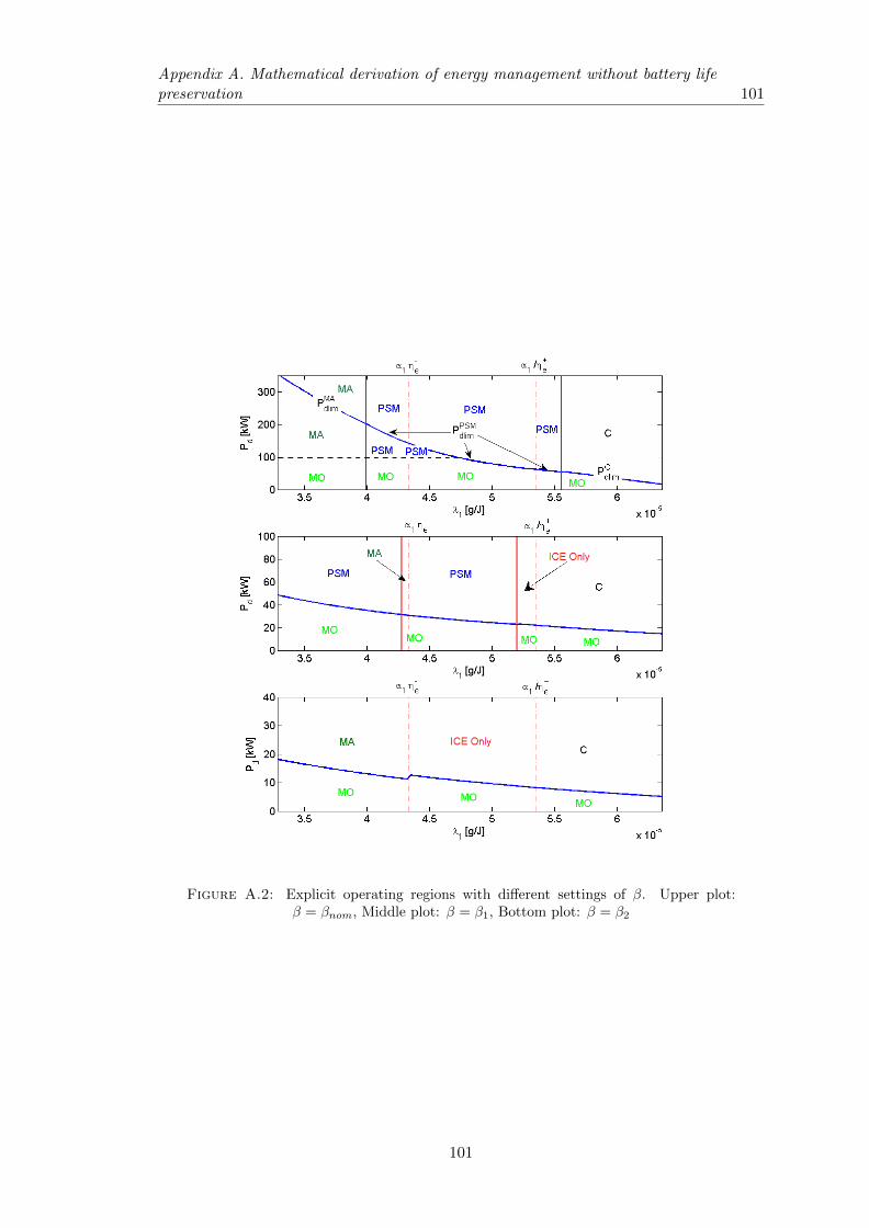
Appendix A. Mathematical derivation of energy management without battery lifepreservation 101
Figure A.2: Explicit operating regions with different settings of β. Upper plot:β = βnom, Middle plot: β = β1, Bottom plot: β = β2
101

Appendix B
Mathematical derivation of
integrated energy management
with battery life preservation
B.1 Optimal battery power in MA and C mode for IEM1
Regarding minPb∈[Pb,0)
HMA, the battery power Pb which minimizes HMA is obtained by
solving the equation ∂HMA∂Pb
= 0. We have,
α1η−e − λo1 (1− 2βPb) + 2λo2αbPb = 0 (B.1)
for Pb ∈[Pb, 0
). As a result, the optimal battery power in the MA mode is achieved as
P ob = PMAb = min
(max
(Pb,
λo1 − α1η−e
2 (λo1β + λo2αb)
), 0
)(B.2)
In terms of minPb∈(0,Pb]
HC , the battery power Pb minimizing HC is computed from solving
the equation ∂HC∂Pb
= 0 . We have,
α1
η+e− λo1 (1− 2βPb) + 2λo2αbPb = 0 (B.3)
for Pb ∈(0, Pb
]. Subsequently, the optimal battery power in the C mode is derived as
P ob = PCb = max
(min
(Pb,
λo1 − α1
η+e
2 (λo1β + λo2αb)
), 0
)(B.4)
103
B.2. Hamiltonian function minimization for IEM1 104
B.2 Hamiltonian function minimization for IEM1
It is obvious that the solution of (B.1)
Pb =λo1 − α1η
−e
2 (λo1β + λo2αb)< 0 (B.5)
for all 0 < λo1 < α1η−e and λo2 ≥ 0. The solution of (B.3)
Pb =λo1 − α1
η+e
2 (λo1β + λo2αb)> 0 (B.6)
for all λo1 >α1
η+eand λo2 ≥ 0. Owing to these observations, for all λo2 ≥ 0, the Hamiltonian
function H is analyzed for three intervals of λo1 namely, (0, α1η−e ), [α1η
−e ,
α1
η+e],(α1
η+e,+∞
).
• For 0 < λo1 < α1η−e :
In this interval, the first derivative of HC with respect to Pb satisfies
∂HC
∂Pb> 0, ∀Pb > 0 (B.7)
Therefore
HC > limPb→0+
HC = HICEonly (B.8)
Moreover, since PMAb < 0, we have
HoMA < lim
Pb→0−HMA = HICEonly (B.9)
From (B.8) and (B.9), the following property is derived
HoMA < HICEonly < HC for 0 < λo1 < α1η
−e andPd > 0 (B.10)
• For α1η−e ≤ λo1 ≤ α1
η+e
In this interval, we have
∂HMA
∂Pb< 0, ∀Pb < 0 (B.11)
∂HC
∂Pb> 0, ∀Pb > 0 (B.12)
104
Appendix B. Mathematical derivation of integrated energy management with battery lifepreservation 105
Hence,
HC > limPb→0+
HC = HICEonly (B.13)
HMA > limPb→0−
HMA = HICEonly (B.14)
for all λ1 ∈[α1η
−e ,
α1
η+e
]and Pd > 0.
• For λo1 >α1
η+e:
The following property holds for λo1 >α1
η+e,
∂HMA
∂Pb< 0, ∀Pb < 0 (B.15)
Therefore,
HMA > limPb→0−
HMA = HICEonly (B.16)
Moreover, since PCb > 0 for λ1 >α1
η+e, we have
HoC < lim
Pb→0−HC = HICEonly (B.17)
Equations (B.16) and (B.17) imply
HoC < HICEonly < HMA for λ1 >
α1
η+eandPd > 0 (B.18)
Moreover, by solving (3.47)-(3.53), it is straight forward to obtain the following proper-
ties: HoMA ≥ HMO for 0 < Pd ≤ PMA
dlim
HoMA ≥ HPSM forg0 ≥ gMA
0
(B.19)
HICEonly ≥ HMO for 0 < Pd ≤ P ICEonlydlim
HICEonly ≥ HPSM forg0 ≥ gICEonly0
(B.20)
HoC ≥ HMO for 0 < Pd ≤ PCdlim
HoC ≥ HPSM forg0 ≥ gC0
(B.21)
HPSM ≥ HMO for 0 < Pd ≤ PPSMdlim (B.22)
105
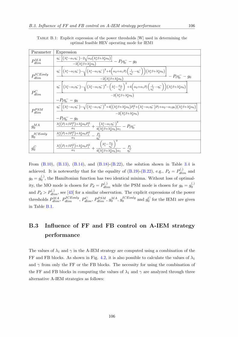
B.3. Influence of FF and FB control on A-IEM strategy performance 106
Table B.1: Explicit expression of the power thresholds [W] used in determining theoptimal feasible HEV operating mode for IEM1
Parameter Expression
PMAdlim
η−e[(λo1−α1η
−e )−2
√α2(λo1β+λo2αb)
]−2(λo1β+λo2αb)
− Plη−e − g0
P ICEonlydlim
η−e
[(λo1−α1η
−e )−
√(λo1−α1η
−e )
2+4
(α2+α1Pl
(1
η+e−η−e
))(λo1β+λo2αb)
]−2(λo1β+λo2αb)
− Plη−e − g0
PCdlim
η−e
(λo1−α1η−e )−
√(λo1−α1η
−e )
2−(λo1−
α1
η+e
)2
+4
(α2+α1Pl
(1
η+e−η−e
))(λo1β+λo2αb)
−2(λo1β+λo2αb)
−Plη−e − g0
PPSMdlim
η−e
[(λo1−α1η
−e )−
√(λo1−α1η
−e )
2+4((λo1β+λo2αb)P 2
l +(λo1−α1η−e )Pl+α2−α1g0)(λo1β+λo2αb)
]−2(λo1β+λo2αb)
−Plη−e − g0
gMA0
λo1(Pl+βP 2l )+λo2αbP
2l
α1+
(λo1−α1η−e )
2
4(λo1β+λo2αb)α1− Plη−e
gICEonly0
λo1(Pl+βP 2l )+λo2αbP
2l
α1− Pl
η+e
gC0λo1(Pl+βP 2
l )+λo2αbP2l
α1+
(λo1−
α1
η+e
)2
4(λo1β+λo2αb)α1− Pl
η+e
From (B.10), (B.13), (B.14), and (B.18)-(B.22), the solution shown in Table 3.4 is
achieved. It is noteworthy that for the equality of (B.19)-(B.22), e.g., Pd = P(.)dlim and
g0 = g(.)0 , the Hamiltonian function has two identical minima. Without loss of optimal-
ity, the MO mode is chosen for Pd = P(.)dlim while the PSM mode is chosen for g0 = g
(.)0
and Pd > P(.)dlim, see [43] for a similar observation. The explicit expressions of the power
thresholds PMAdlim, P ICEonlydlim , PCdlim, PPSMdlim , gMA
0 , gICEonly0 and gC0 for the IEM1 are given
in Table B.1.
B.3 Influence of FF and FB control on A-IEM strategy
performance
The values of λ1 and γ in the A-IEM strategy are computed using a combination of the
FF and FB blocks. As shown in Fig. 4.2, it is also possible to calculate the values of λ1
and γ from only the FF or the FB blocks. The necessity for using the combination of
the FF and FB blocks in computing the values of λ1 and γ are analyzed through three
alternative A-IEM strategies as follows:
106
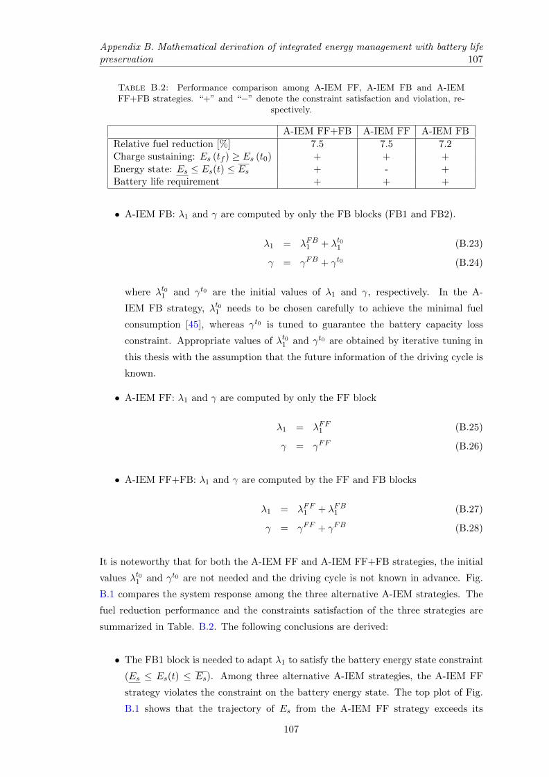
Appendix B. Mathematical derivation of integrated energy management with battery lifepreservation 107
Table B.2: Performance comparison among A-IEM FF, A-IEM FB and A-IEMFF+FB strategies. “+” and “−” denote the constraint satisfaction and violation, re-
spectively.
A-IEM FF+FB A-IEM FF A-IEM FB
Relative fuel reduction [%] 7.5 7.5 7.2Charge sustaining: Es (tf ) ≥ Es (t0) + + +
Energy state: Es ≤ Es(t) ≤ Es + - +Battery life requirement + + +
• A-IEM FB: λ1 and γ are computed by only the FB blocks (FB1 and FB2).
λ1 = λFB1 + λt01 (B.23)
γ = γFB + γt0 (B.24)
where λt01 and γt0 are the initial values of λ1 and γ, respectively. In the A-
IEM FB strategy, λt01 needs to be chosen carefully to achieve the minimal fuel
consumption [45], whereas γt0 is tuned to guarantee the battery capacity loss
constraint. Appropriate values of λt01 and γt0 are obtained by iterative tuning in
this thesis with the assumption that the future information of the driving cycle is
known.
• A-IEM FF: λ1 and γ are computed by only the FF block
λ1 = λFF1 (B.25)
γ = γFF (B.26)
• A-IEM FF+FB: λ1 and γ are computed by the FF and FB blocks
λ1 = λFF1 + λFB1 (B.27)
γ = γFF + γFB (B.28)
It is noteworthy that for both the A-IEM FF and A-IEM FF+FB strategies, the initial
values λt01 and γt0 are not needed and the driving cycle is not known in advance. Fig.
B.1 compares the system response among the three alternative A-IEM strategies. The
fuel reduction performance and the constraints satisfaction of the three strategies are
summarized in Table. B.2. The following conclusions are derived:
• The FB1 block is needed to adapt λ1 to satisfy the battery energy state constraint
(Es ≤ Es(t) ≤ Es). Among three alternative A-IEM strategies, the A-IEM FF
strategy violates the constraint on the battery energy state. The top plot of Fig.
B.1 shows that the trajectory of Es from the A-IEM FF strategy exceeds its
107
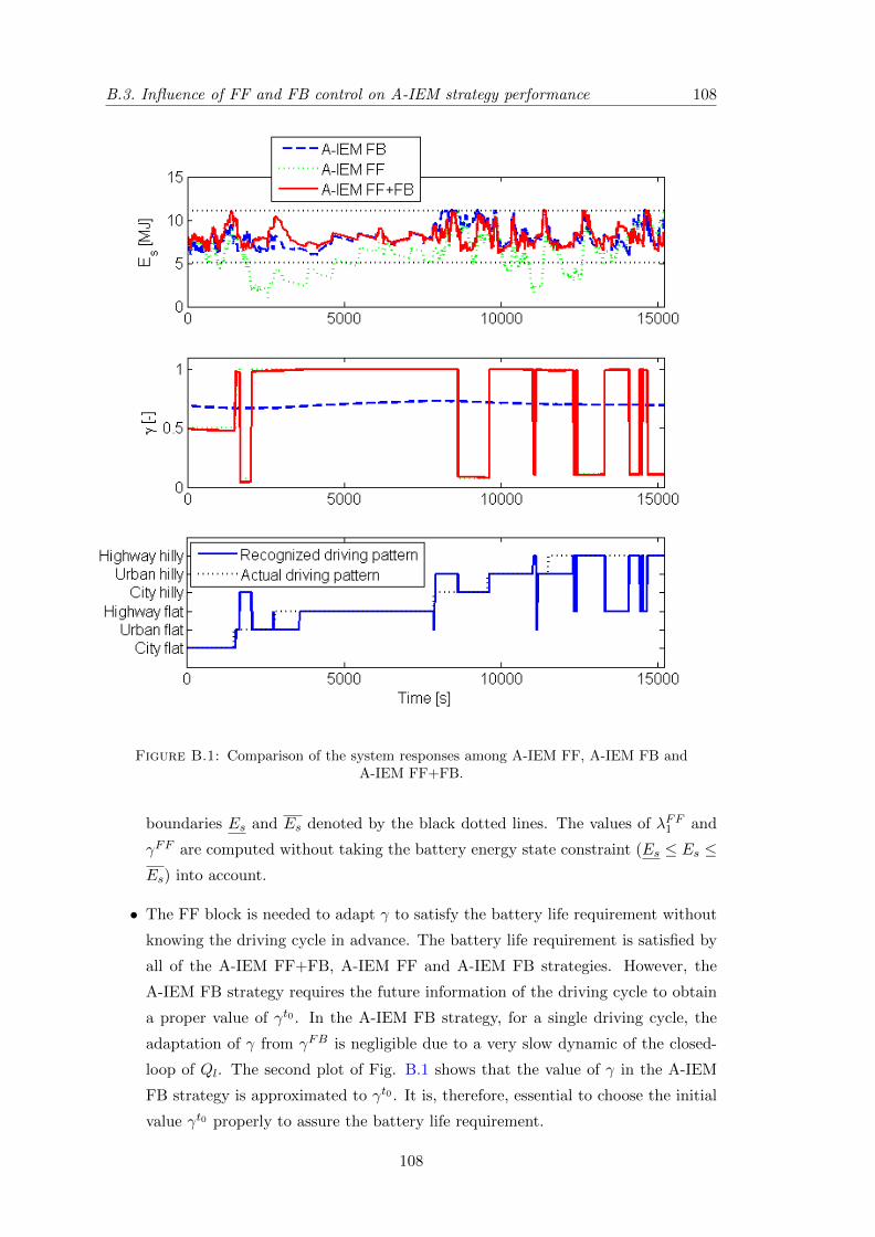
B.3. Influence of FF and FB control on A-IEM strategy performance 108
Figure B.1: Comparison of the system responses among A-IEM FF, A-IEM FB andA-IEM FF+FB.
boundaries Es and Es denoted by the black dotted lines. The values of λFF1 and
γFF are computed without taking the battery energy state constraint (Es ≤ Es ≤Es) into account.
• The FF block is needed to adapt γ to satisfy the battery life requirement without
knowing the driving cycle in advance. The battery life requirement is satisfied by
all of the A-IEM FF+FB, A-IEM FF and A-IEM FB strategies. However, the
A-IEM FB strategy requires the future information of the driving cycle to obtain
a proper value of γt0 . In the A-IEM FB strategy, for a single driving cycle, the
adaptation of γ from γFB is negligible due to a very slow dynamic of the closed-
loop of Ql. The second plot of Fig. B.1 shows that the value of γ in the A-IEM
FB strategy is approximated to γt0 . It is, therefore, essential to choose the initial
value γt0 properly to assure the battery life requirement.
108
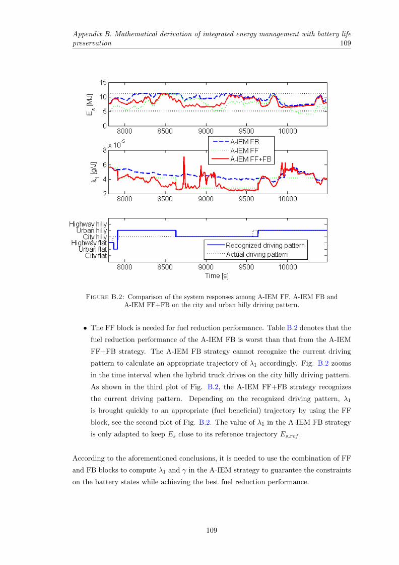
Appendix B. Mathematical derivation of integrated energy management with battery lifepreservation 109
Figure B.2: Comparison of the system responses among A-IEM FF, A-IEM FB andA-IEM FF+FB on the city and urban hilly driving pattern.
• The FF block is needed for fuel reduction performance. Table B.2 denotes that the
fuel reduction performance of the A-IEM FB is worst than that from the A-IEM
FF+FB strategy. The A-IEM FB strategy cannot recognize the current driving
pattern to calculate an appropriate trajectory of λ1 accordingly. Fig. B.2 zooms
in the time interval when the hybrid truck drives on the city hilly driving pattern.
As shown in the third plot of Fig. B.2, the A-IEM FF+FB strategy recognizes
the current driving pattern. Depending on the recognized driving pattern, λ1
is brought quickly to an appropriate (fuel beneficial) trajectory by using the FF
block, see the second plot of Fig. B.2. The value of λ1 in the A-IEM FB strategy
is only adapted to keep Es close to its reference trajectory Es ref .
According to the aforementioned conclusions, it is needed to use the combination of FF
and FB blocks to compute λ1 and γ in the A-IEM strategy to guarantee the constraints
on the battery states while achieving the best fuel reduction performance.
109
B.4. Benefit and cost for battery usage in MA, MO and R mode 110
B.4 Benefit and cost for battery usage in MA, MO and R
mode
To transform the cost and benefit when using the battery to [e/s], it is essential to
define the diesel price πf [e/g] and a lifetime dependence battery capacity loss price
πb [e/%]. πf = πdieselρ is obtained from the worldwide diesel price πdiesel [e/liter] and
the diesel density ρ [g/liter]. Regarding the battery capacity loss price πb, Eq. (2.24),
Ql = h (Ps, Tb)Qz−1z
l , shows that for a fixed value of Ps and Tb, the incremental battery
capacity loss Ql is smaller for higher Ql since z = 0.552 < 1. It suggests that πb should
also depend on Ql to equally justify the cost from Ql over its lifetime. As a result, πb is
computed from the following equation
πb(t)h (Ps(t), Tb(t))Qz−1z
l (t) = Πbh (Ps(t), Tb(t))Qz−1z
EoL (B.29)
where Πb [e/%] equals to a new battery pack price excluding the costs for the battery
thermal management system. The right hand side of (B.29) expresses that at the end of
the battery lifetime, each usage of the battery has to pay a price of Πb since the battery
needs to be replaced afterward. From (B.29), we have
πb(t) = Πb(Ql(t)
QEoL)1−zz (B.30)
To compute the benefit and cost from using the battery in MA, MO and R mode, the
analysis makes use of the developed vehicle model in combination with the predefined
prices πf and πb.
The fuel consumption of the ICE in the ICE Only mode to propel the truck and supply
the reefer trailer is
mICEonlyf = α1
(Pd +
Pl
η+e
+ g0
)+ α2 (B.31)
The fuel consumed by the ICE in MA mode with the battery discharge power Pb < 0 is
obtained as
mMAf = α1
(Pd + η−e (Pb + Pl) + g0
)+ α2 (B.32)
Hence, the benefit achieved from using the MA mode is derived as
bMA = πf (mICEonlyf − mMA
f ) = πfα1
(−Pbη−e + Pl
(1
η+e− η−e
))(B.33)
110
Appendix B. Mathematical derivation of integrated energy management with battery lifepreservation 111
Similarly, the benefit from using the MO mode, with the battery discharge power Pb < 0,
is obtained as
bMO = πfα1
(−Pbη−e + Pl
(1
η+e− η−e
))+ α2 (B.34)
The cost from the battery capacity loss for both MA and MO mode is computed as
cMA = cMO = πbh(Pb − βP 2
b , Tb)Q
z−1z
l (B.35)
Regarding the R mode, the cost from absorbing the braking energy with the battery
charge power Pb > 0 is
cR = 2πbh(Pb − βP 2
b , Tb)Q
z−1z
l (B.36)
The benefit from using the absorbed energy in MO mode is
bR = πfα1
(−P ′bη−e + Pl
(1
η+e− η−e
))+ α2 (B.37)
with P′b = arg
P′b<0
(P′b − β
(P′b
)2= −(Pb − βP 2
b )
)is the battery discharge power at its
terminals corresponding to the net retrieved battery power Pb − βP 2b .
From (B.33)-(B.37), the powers P l,MAcb , P l,MO
cb and P ucb are computed as
P l,MAcb = arg min
Pb∈[−120e3,0]Pb| bMA − cMA ≥ 0 (B.38)
P l,MOcb = arg min
Pb∈[−120e3,0]Pb| bMO − cMO ≥ 0 (B.39)
P ucb = arg maxPb∈[0,120e3]
Pb| bR − cR ≥ 0 (B.40)
Remark 7. Without assuming that the net retrieved battery energy from the R mode
will be used in the MO mode with the same power pattern, the benefit from fuel reduction
when absorbing the braking energy can be computed as follows.
If the battery energy is discharged with an amount of Es1, the battery has to be charged
by means of the ICE and/or braking energy to re-fill the battery with an amount of at
least Es1 to guarantee the charge sustaining constraint. When discharging the battery,
λ1 represents an equivalent fuel cost to recharge the battery energy using the ICE. If
there is free braking energy, this fuel cost is reduced by absorbing the braking energy
to recharge the battery. Owing to this observation, the benefit (from fuel reduction)
when absorbing the braking energy can be estimated as follows. At every time instant
t, an averaged value λ1 avg of λ1 over a past period [t − τλ1 , t] is computed and used
as the future cost of the electric power. τλ1 > 0 is a predefined value. Since the fuel
mass flow mf of the ICE depends linearly on the ICE power, the benefit from fuel
111
B.5. Computation of battery capacity loss upper bound 112
reduction according to charging the battery from braking energy with a power of Pb can
be estimated as
bR = πfλ1 avgP′b (B.41)
with P′b = arg
P′b<0
(P′b − β
(P′b
)2= −(Pb − βP 2
b )
)is the battery discharge power at its
terminals corresponding to the net retrieved battery power Pb − βP 2b .
B.5 Computation of battery capacity loss upper bound
The static battery cycle-life model (2.22), Ql = B (Crate) e−Ea(Crate)R(Tb+273)
(E
nVoc3600
)z, suggests
that for specific Ql, E and a constant battery Crate, there exists a constant battery
temperature Tb such that the equation (2.22) is satisfied. As a result, given the time-
varying Ps and Tb satisfying (Ql(tf ) ≤ Ql), there exists a constant Tb and Ps such
that
Ql(tf ) = B(Crate
)e−Ea(Crate)
RTb
(E (tf )
nVoc3600
)z(B.42)
where Ql(tf ) = Ql (t0) +tf∫t0
Ql (Ps, Tb, τ) dτ , and Crate corresponds to an average battery
charged/discharged power Ps = 1tf−t0
tf∫t0
|Ps (τ)| dτ .
Owing to the assumption that the truck runs on a same route for the entire battery life,
the following equation is obtained
Ql (tEoL) = B(Crate
)e−Ea(Crate)
RTb
(E (tf ) tEoL−t0tf−t0nVoc3600
)z(B.43)
Let Ql(tf ) = Ql and Ql(tEoL) = Ql EoL. From (B.42) and (B.43), the value of Ql is
derived as
Ql =Ql EoL(tEoL−t0tf−t0
)z (B.44)
112
Bibliography
[1] M. van der Hoeven. CO2 emssions from fuel combustion, highlights. Technical
report, International Energy Agency, 2012.
[2] NRC. Understanding and responding to climate change. Technical report, Board
on Atmospheric Sciences and Climate, US National Academy of Sciences, 2008.
[3] N. Oreskes. Beyond the ivory tower: The scientific consensus on climate change.
Science, 306(5702), 2004.
[4] K.J. Fender and D. A. Pierce. An analysis of the operational costs of trucking: 2012
update. Technical report, American Transportation Research Institute, Sep 2012.
[5] H. Zhao, A. Burke, and L. Zhu. Analysis of class 8 hybrid-electric truck technologies
using diesel, LNG, electricity, and hydrogen, as the fuel for various applications.
In Proc. of EVS27 International Battery, Hybrid and Fuel Cell Electric Vehicle
Symposium, Barcelona, Spain, 17-20 Nov 2013.
[6] T.H. Bradley and A.A. Frank. Design, demonstrations and sustainability impact
assessments for plug-in hybrid electric vehicles. Renewable and Sustainable Energy
Reviews, 13:115–128, 2009.
[7] N. Dressler, W. Bernhart, J. Shen, S. Keese, A. Fernandez, and F. Pietras. Truck
powertrain 2020, mastering the CO2 challenge. Technical report, Roland Berger,
2009.
[8] R. Maier. Improving energy efficiency of commercial vehicles. Technical report,
EVP Engineering, Robert Bosch GmbH, Brasil, Aug 2013.
[9] G.J.C.M. Arts. Hybrid technology for heavy duty trucks. In Proc. of 21st Aachen
Colloquium Automobile and Engine Technology, 2012.
[10] C. Vyas and D. Hurst. Electric vehicle consumer survey. Consumer attitudes, opin-
ions, and preferences for electric vehicles and EV charging stations. Technical
report, Navigant Research, 2013.
113
Bibliography 114
[11] M.S. Alam. Key barriers to the profitable commercialization of plug-in hybrid
and electric vehicles. Adv Automob Eng, 2(2):1–2, 2013. doi: 10.4172/2167-7670.
1000e117.
[12] A review of battery technologies for automotive applications. Technical report,
EUROBAT and ACEA and JAMA and KAMA and ILA, 2014.
[13] L. Browning and S. Unnasch. Hybrid electric vehicle commercialization issues. In
Applications and Advances, 2001. The Sixteenth Annual Battery Conference on,
pages 45–45, 2001. doi: 10.1109/BCAA.2001.905098.
[14] P. Svens, J. Lindstom, M. Behm, and G. Lindbergh. HEV lithium-ion battery test-
ing and driving cycle analysis in a heavy-duty truck field study. ECS Transactions,
41(32):13–26, 2012.
[15] J.T.B.A. Kessels, M. Koot, B. de Jager, P. P.J. van den Bosch, N.P.I. Aneke,
and D. B. Kok. Energy management for the electric powernet in vehicles with a
conventional drivetrain. IEEE Trans on Control Systems Tech, 15(3):494–505, May
2007.
[16] Vital van Reeven, Theo Hofman, Frank Willems, Rudolf Huisman, and Maarten
Steinbuch. Optimal control of engine warmup in hybrid vehicles. Oil & Gas Science
and Technology, Dec 2014. doi: http://dx.doi.org/10.2516/ogst/2014042.
[17] V. van Reeven, R.G.M. Huisman, J.T.B.A. Kessels, T.H. Pham, and T. Hofman.
Integrating energy and thermal management of hybrid trucks. In Proc. of the 12th
International Conference on Commercial Vehicles Truck, Bus, Van, Trailer, pages
1–14, Celle, Germany, 5-6 June 2013.
[18] C. Kuper, M. Hoh, G. Houchin-Miller, and J. Fuhr. Thermal management of hybrid
vehicle battery systems. In EVS24, Stavanger, Norway, May 13-16 2009.
[19] K. Buford, J. Williams, and M. Simonini. Determining most energy efficient cooling
control strategy of a rechargeable energy storage system. In Proc. of the SAE World
Congress, December 2011. SAE Paper 2011-01-0893.
[20] T.H. Pham, J.T.B.A. Kessels, P.P.J. van den Bosch, R.G.M. Huisman, and
R.M.P.A. Nevels. On-line energy and battery thermal management for hybrid elec-
tric heavy-duty truck. In Proc. of the American Control Conf., Washington, DC,
June 2013.
[21] M. Ecker, J.B. Gerschler, J. Vogel, S. Kabitz, F. Hust, P. Dechent, and D.U. Sauer.
Development of a lifetime prediction model for lithium-ion batteries based on ex-
tended accelerated aging test data. Journal of Power Sources, 215:248–257, 2012.
114
Bibliography 115
[22] A. Sciarretta and L. Guzzella. Control of hybrid electric vehicles. IEEE Control
Systems Magazine, 27(2):60–70, April 2007.
[23] B. de Jager, T. van Keulen, and J.T.B.A. Kessels. Optimal Control of Hybrid
Vehicles. Springer, 2013.
[24] A.A. Malikopoulos. Supervisory power management control algorithms for hybrid
electric vehicles: A survey. IEEE Trans on Intelligent Transportation Systems, 15
(5):1869 – 1885, 2014.
[25] B.M. Baumann, G. Washington, B.C. Glenn, and G. Rizzoni. Mechatronic design
and control of hybrid electric vehicles. IEEE/ASME Trans Mechatronics, 5(1):
58–72, Mar 2000.
[26] H. Wallentowitz and R. Ludes. System control application for hybrid vehicles. In
Proc. of the IEEE Conference on Control Applications, volume 1, pages 639–650,
Glasgow, 24-26 Aug 1994.
[27] N. Jalil, N.A. Kheir, and M. Salman. A rule-based energy management strategy for
a series hybrid vehicle. In Proc. of the American Control Conf., volume 1, pages
689–693. Albuquerque, NM, 4-6 Jun 1997.
[28] T. Hofman, M. Steinbuch, R. van Druten, and A. Serrarens. Rule-based energy
management strategies for hybrid vehicles. Int. J. Electric and Hybrid Vehicles, 1
(1):71–94, 2007.
[29] E.D. Tate and S.P. Boyd. Finding ultimate limits of performance for hybrid electric
vehicles. SAE Paper, (2000-01-3099), 2000.
[30] T.C.J. Romijn, M.C.F. Donkers, J.T.B.A. Kessels, and S. Weiland. A dual decom-
position approach to complete energy management for a heavy-duty vehicle. In
Proc. of IEEE Conference on Decision and Control, Los Angeles, CA, 15-17 Dec
2014.
[31] O. Sundstrom, L. Guzzella, and P. Soltic. Optimal hybridization in two parallel
hybrid electric vehicles using dynamic programming. In Proc. 17th World Congr.
int. Fed. Autom. Control, pages 4642–4647, 2008.
[32] F. Kirschbaum, M. Back, and M. Hart. Determination of the fuel-optimal trajectory
for a vehicle along a known route. In Proc. 15th IFAC World Congr, volume 15,
2002.
[33] C.-C. Lin, H. Peng, J.W. Grizzle, and J.-M. Kang. Power management strategy for
a parallel hybrid electric truck. IEEE Trans. Control Syst. Technol, 11(6):839–849,
2003.
115
Bibliography 116
[34] C. Guardiola, B. Pla, S. Onori, and G. Rizzoni. Insight into the HEV/PHEV opti-
mal control solution based on a new tuning method. Control Engineering Practice,
29:247–256, Aug 2014.
[35] P. Pisu and G. Rizzoni. A comparative study of supervisory control strategies for
hybrid electric vehicles. IEEE Trans on Control Systems Tech., 15(3):506–518, May
2007.
[36] B. Sampathnarayanan, S. Onori, and S. Yurkovich. An optimal regulation strat-
egy with disturbance rejection for energy management of hybrid electric vehicles.
Automatica, 50(1):128–140, Jan 2014.
[37] S. Delprat, J. Lauber, T.M. Guerra, and J. Rimaux. Control of a parallel hybrid
powertrain: Optimal control. IEEE Trans on Vehicular Tech, 53(3):872–881, May
2004.
[38] L. Guzzella and A. Sciarretta. Vehicle Propulsion Systems - Introduction to Mod-
eling and Optimization. Springer-Verlag, Berlin Heidelberg, 2nd edition, 2007.
[39] M. Koot, J.T.B.A. Kessels, B. de Jager, W.P.M.H. Heemels, P.P.J. van den Bosch,
and M. Steinbuch. Energy management strategies for vehicular electric power sys-
tems. IEEE Trans on Vehicular Tech, 54(3):771–782, May 2005.
[40] M.W.T. Koot. Energy Management for vehicular electric power systems. PhD the-
sis, Dept. Mech. Eng., Technische Univ. Eindhoven, Eindhoven, The Netherlands,
2006.
[41] C. Musardo, G. Rizzoni, and B. Staccia. A-ECMS: An adaptive algorithm for
hybrid electric vehicle energy management. In Proc. of the Joint 44th IEEE Conf.
Decision Control, Eur. Control Conf., pages 1816–1823, Seville, Spain, December
2005.
[42] J.T.B.A. Kessels, M.W.T. Koot, P.P.J. van den Bosch, and D.B. Kok. Online
energy management for hybrid electric vehicles. IEEE Trans on Vehicular Tech,
57(6):3428–3440, November 2008.
[43] D. Ambuhl, O. Sundstrom, A. Sciarretta, and L. Guzzella. Explicit optimal con-
trol policy and its practical application for hybrid electric powertrains. Control
Engineering Practice, 18(12):1429–1439, 2010.
[44] J.T.B.A. Kessels. Energy Management for Automotive Power Nets. PhD thesis,
Technische Universiteit Eindhoven, 2007.
[45] T. van Keulen. Fuel Optimal Control of Hybrid Vehicles. PhD thesis, Eindhoven
University of Technology, 2011.
116
Bibliography 117
[46] A. Sciarretta, L. Serrao, P.C. Dewangan, P. Tona, E.N.D. Bergshoeff, C. Bordons,
L. Charmpa, Ph. Elbert, L. Eriksson, T. Hofman, M. Hubacher, P. Isenegger, F. La-
candia, A. Laveau, H. Li, D. Marcos T. Nuesch, S. Onori, P. Pisu, J. Rios, E. Silvas,
M. Sivertsson, L. Tribioli, A.-J. van der Hoeven, and M. Wu. A control benchmark
on the energy management of a plug-in hybrid electric vehicle. Control Engineering
Practice, 29:287–298, 2014.
[47] H.P. Geering. Optimal Control with Engineering Applications. Springer-Verlag
Berlin Heidelberg, 2007.
[48] J.T.B.A. Kessels, J.H.M. Martens, P.P.J. van den Bosch, and W.H.A. Hendrix.
Smart vehicle powernet enabling complete vehicle energy management. In Proc.
of the IEEE Vehicle Power and Propulsion Conference(VPPC), Seoul, Korea, 9-12
Oct 2012.
[49] L. Serrao. Open issues in supervisory control of hybrid electric vehicles: a unified
approach using optimal control methods. In Proc. RHEVE, 2011.
[50] J. Lescot, A. Sciarretta, Y. Chamaillard, and A. Charlet. On the integration of
optimal energy management and thermal management of hybrid electric vehicles.
In Proc. of the Vehicle Power and Propulsion Conference (VPPC), Lille, 1-3 Sept
2010.
[51] J.T.B.A. Kessels, F.P.T. Willems, W.J. Schoot, and P.P.J. van den Bosch. Inte-
grated energy and emission management for hybrid electric truck with SCR af-
tertreatment. In Proc. of the IEEE Vehicle Power and Propulsion Conference
(VPPC), Lille, France, September 2010.
[52] F. Willems, F. Kupper, and R. Cloudt. Integrated powertrain control for optimal
CO2-NOx tradeoff in an Euro-VI diesel engine with waste heat recovery system. In
Proc. of the American Control Conference, Montreal, Canada, June 27-29 2012.
[53] P. Klaus, A. Martin, H. Josef, W. Martin, and N. Heimo. Simulation and energy
management of hybrid commercial vehicles with attention to the thermal system
behaviour. In Proc. of the FISTA World Automotive Congress, Budapest, Hungary,
30 May - 4 June. 2010.
[54] H.T. Pham, P.P.J. van den Bosch, J.T.B.A. Kessels, and R.G.M. Huisman. In-
tegrated energy and thermal management for hybrid electric heavy duty trucks.
In Proc. of the IEEE Vehicle Power and Propulsion Conference (VPPC), Seoul,
Korea, 9-12 October 2012.
[55] L. Johannesson, N. Murgovski, S. Ebbesen, B. Egardt, E. Gelso, and J. Hellgren.
Including a battery state of health model in the hev component sizing and optimal
117
Bibliography 118
control problems. In Proc. of the 7th IFAC Symposium on Advances in Automotive
Control, Tokyo, Japan, September 4-7 2013.
[56] T.-H. Wang, O. Sename, and J.J. Martinez-Molina. A LPV/H∞ approach for fuel
consumption minimization of the phev with battery life prolongation. In Proc.
of the 7th IFAC Symposium on Advances in Automotive Control, Tokyo, Japan,
September 4-7 2013.
[57] T.M. Padovani, M. Debert, G. Colin, and Y. Chamaillard. Optimal energy man-
agement strategy including battery health through thermal management for hybrid
vehicles. In Proc. of the 7th IFAC Symposium on Advances in Automotive Control,
Tokyo, Japan, September 4-7 2013.
[58] L. Serrao, S. Onori, A. Sciarretta, Y. Guezennec, and G. Rizzoni. Optimal energy
management of hybrid electric vehicles including battery aging. In Proc. of the
American Control Conf., San Francisco, CA, USA, June 29 - July 01. 2011.
[59] S. Ebbesen, P. Elbert, and L. Guzzella. Battery state-of-health perceptive energy
management for hybrid electric vehicles. IEEE Trans on Control Systems Tech, 61
(7):2893–2900, September 2012.
[60] T.H. Pham, J.T.B.A. Kessels, P.P.J. van den Bosch, and R.G.M. Huisman. Cost-
effective energy management for hybrid electric heavy-duty truck including battery
aging. In Proc. of the 2013 ASME Dynamic Systems and Control Conference, Palo
Alto, CA, October 21-23 2013.
[61] T.H. Pham, S.K. Ramachandran, J.T.B.A. Kessels, R.G.M. Huisman, and P.P.J.van
den Bosch. Integrating battery management into energy management for hybrid
heavy-duty trucks. In Proc. of the FISITA World Automotive Congress 2014, Maas-
tricht, The Netherlands, 2-6 June 2014.
[62] H. Waschl, I. Kolmanovsky, M. Steinbuch, and L. del Re. Optimization and Optimal
Control in Automotive Systems. Springer, 2014.
[63] T.H. Pham, P.P.J. van den Bosch, J.T.B.A. Kessels, and R.G.M. Huisman. Inte-
grated online energy and battery life management for hybrid long haulage truck.
In Proc. of the IEEE Vehicle Power and Propulsion Conference (VPPC), Coimbra,
Portugal, 9-12 October 2014.
[64] E. Tazelaar, B. Veenhuizen, P.P.J. van den Bosch, and M. Grimminck. Analytical
solution of the energy management for fuel cell hybrid propulsion systems. IEEE
Trans on Vehicular Tech, 61(5):1986–1998, June 2012.
[65] I.T. Jolliffe. Principal Component Analysis. Springer, 2nd edition, 2002.
118
Bibliography 119
[66] V. Pop. Universal State-of-Charge Indication for Portable Applications. PhD thesis,
Universiteit Twente, 2007.
[67] C. Park and A.K. Jaura. Dynamic thermal model of li-ion battery for predictive
behavior in hybrid and fuel cell vehicles. In Proc. of the Future Transportation
Technology Conf., Costa Mesa, California, June 2003. SAE Paper 2003-01-2286.
[68] E. Meissner and G. Richter. The challenge to the automotive battery industry:
the battery has to become an increasingly integrated component within the vehicle
electric power system. Journal of Power Sources, 144:438–460, 2005.
[69] A. Barre, B. Deguilhem, S. Grolleau, M. Gerard, F. Suard, and D. Riu. A review on
lithium-ion battery ageing mechanisms and estimations for automotive applications.
Journal of Power Sources, 241:680–689, 2013.
[70] T. Yuksel and J. Michalek. Development of a simulation model to analyze the effect
of thermal management on battery life. SAE Technical Paper, (2012-01-0671), 2012.
doi: 10.4271/2012-01-0671.
[71] A. Cordoba-Arenas, S. Onori, G. Rizzoni, and G. Fan. Aging propagation in ad-
vanced battery systems: Preliminary results. In Proc. of the 7th IFAC Symposium
on Advances in Automotive Control, Tokyo, Japan, September 4-7 2013.
[72] J. Wang, P. Liu, J. Hicks-Garner, E. Sherman, S. Soukiazian, M. Verbrugge,
H. Tataria, J. Musser, and P. Finamore. Cycle-life model for graphite-LiFePO4
cells. Journal of Power Sources, 196:3942–3948, 2011.
[73] PNGV Battery Test Manual, DOE/ID-10597, Feb 2001.
[74] Richard Vinter. Optimal Control. Systems & control: foundation & applications.
Springer, 2010.
[75] R.F. Hartl, S.P. Sethi, and R.G. Vickson. A survey of the maximum principles for
optimal control problems with state contraints. SIAM Review, 37:181–218, 1995.
[76] T. van Keulen, J. Gillot, B. de Jager, and M. Steinbuch. Solutions for state con-
strained optimal control problems applied to power split control for hybrid vehicles.
Automatica, 50:187–192, 2014.
[77] S.-I Jeon, S.-T Jo, Y.-I Park, and J.-M Lee. Multi-mode driving control of a par-
allel hybrid electric vehicle using driving pattern recognition. Journal of Dynamic
System, Measurement, and Control, 124:141–149, March 2002.
[78] R. Wang and S.M. Lukic. Review of driving conditions prediction and driving
style recognition based control algorithms for hybrid electric vehicles. In Vehicle
119
Bibliography 120
Power and Propulsion Conference (VPPC), 2011 IEEE, pages 1–7, Sept 2011. doi:
10.1109/VPPC.2011.6043061.
[79] H. He, C. Sun, and X. Zhang. A method for indentification of driving patterns
in hybrid electric vehicles based on a LVQ neural network. Energies, 5:3363–3380,
2012. doi: 10.3390/en5093363.
[80] C. Zhang, A. Vahid, P. Pisu, X. Li, and K. Tennant. Role of terrain preview in
energy management of hybrid electric vehicles. IEEE Trans on Vehicular Tech, 59
(3):1139–1147, March 2010.
[81] L. Fu, U. Ozguner, P. Tulpule, and V. Marano. Real-time energy management
and sensitivity study for hybrid electric vehicles. In Proc. of the American Control
Conf., CA, USA, June 29 - July 01 2011.
[82] David C. Lay. Linear Algebra and Its Applications. Addison-Wesley, 4th edition,
2012.
[83] J. Shlens. A tutorial on principal component analysis. Technical report, Institute
for Nonlinear Science, Univeristy of California, San Diego La Jolla, CA, 2005.
[84] S.W. Smith. The Scientist and Engineering’s Guide to Digital Signal Processing.
California Technical, 1997.
[85] A. Khaligh and Z. Li. Battery, ultracapacitor, fuel cell, and hybrid energy storage
systems for electric, hybrid electric, fuel cell, and plug-in hybrid electric vehicles:
State of the art. IEEE Trans on Vehicular Tech, 59(6):2806–2814, July 2010.
[86] V.D. Ngo. Gear Shift Strategies for Automotive Transmissions. PhD thesis, Tech-
nische Universiteit Eindhoven, Sep 2012.
120
Acknowledgments
Doing a PhD is an epic journey which I could not complete without the invaluable
support from many people. To them, I owe my gratitude.
First of all, I am deeply grateful to my first promotor Prof. Paul van den Bosch.
Without his constant guidance, I would never have been able to finish my PhD. His
critical questions during our discussions stimulate me to understand the problem more
explicitly and to explore the problem from numerous aspects, which ultimately improves
the scientific level of my work. Paul is an expert in motivating his students to deal with
challenging tasks. Besides, he is also a great promotor who really takes care of and
supports his students. “Thanks a lot for your faith in me”.
I would like to convey my sincere gratitude to my co-promotor Dr. John Kessels who
spends every week his precious time discussing and guiding me. His fruitful advices
undoubtedly play a major role in the completion of my PhD. I truly appreciate all the
industrial experiences he shares with me in our meeting. I have learnt from John lots
of valuable lessons to broaden my academic knowledge and to work effectively in the
industry. “Thanks a great deal for your inspiring ideas and extensive knowledge of
energy management in the automotive power net”.
I owe a lot of thanks to the doctoral committee members Prof. Edward Holweg, Prof.
Alain Bouscayrol, Prof. Maarten Steinbuch, Prof. Bram de Jager, Dr. Rudolf Huisman
and Prof. Ton Backx for their approval on my thesis. Thanks a lot for spending your
time reviewing this thesis and providing me relevant feedback to further improve its
readability and clarity.
My gratitude also falls towards the colleagues at DAF Trucks N.V. for their cooperation
and willingness to share their knowledge. My thankfulness, in particular, goes to Dr.
Rudolf Huisman who has been the co-author for all of my publication so far. He always
provides me constructive comments and remarks on my paper. He is also very nice
colleague at DAF Trucks N.V., being willing to support and to help me whenever I ask
for help. Certainly, I am really enjoying working with him.
Furthermore, I would like to convey my thanks to the colleagues in the Control Systems
group. It has been my pleasure to work in a very relaxing and friendly atmosphere.
121
Bibliography 122
Particularly, I really enjoy playing football for the “Team of Rob”. Thanks Constantijn,
Handian, Hernan, Koen, Michel, Pepijn, Quang, Rian, Tuan, Veaceslav, Mohammed,
Mohsin, Rob, Mark, Andelko, Mircea, etc., for sharing the great spirit of the team.
I want to extend my warm thanks to the PhD students in the HIT project, Vital, Yanja
and Emilia, for all the fruitful discussions and cooperation.
Above all, I owe my deep gratitude to my parents, brothers (and their families) for their
unconditional support during my study abroad. I thank my brother, Duc, for motivating
me to start the PhD study. “Thank you for all your invaluable advices when we are
both away from home for study”.
Finally, I would like to dedicate my special and heartfelt thanks to my beloved wife,
Huong, for her endless love and constant support. Thanks for your great encouragement
to stimulate me in finishing my PhD. Thanks for your heartfelt sympathy with me during
my PhD life. Thanks for sharing every happy and stressful moment on my PhD journey.
Together with my wife, my beloved son, Hai, are my eternal energy sources. Seeing his
smile and playing with him reveal all the working pressure. Without my wife and my
son, I would never finish this epic PhD journey successfully.
122
Curriculum Vitae
Pham Hong Thinh was born on 18th February 1986 in Bac Ninh, VietNam. He gradu-
ated from Hanoi University of Technology, VietNam in 2008. After that, he studied his
Master degree in the System Theoretic Analysis and Control Lab, Electrical Engineering
Department, KAIST, Korea. During his Master study, he focused on analyzing stability
of nonlinear systems and developing nonlinear controllers to stabilize a class of nonlinear
systems affected by exogenous signals and time-delay. His Master work was presented
in the thesis entitled “A Study on Robust Gain Scheduling in Nonlinear Systems with
Exogenous Signal and Time-Delay in the Input”. After receiving the Master diploma in
2010, he went back to VietNam and worked for a Robotic Company (TOSY) in Viet-
Nam as a Control/Software engineer. In May 2011, he was appointed as a PhD student
in the Control Systems group of the Electrical Engineering department at Eindhoven
University of Technology. His research deals with integrated energy management for hy-
brid electric vehicles, being part of a Dutch multidisciplinary research project entitled:
“Hybrid Innovations for Trucks (HIT)”. The results of this research are presented in this
thesis.
During his PhD research, Thinh obtained the DISC certificate for fulfilling the course
program requirements of the Dutch Institute for Systems and Control. He also received
the best paper prize at the Vehicle Power and Propulsion Conference 2014 in Coimbra,
Portugal.
123