INTEGRATED DIRECT/INDIRECT ADAPTIVE ROBUST CONTROL OF MULTI-DOFHYDRAULIC ROBOTIC ARMS ∗

Amit MohantyGraduate Student

School of Mechanical EngineeringPurdue University

West Lafayette, IN-47906Email: amohanty@purdue.edu

Bin YaoProfessor

School of Mechanical EngineeringPurdue University

West Lafayette, IN-47906Email: byao@purdue.edu

Proceedings of IMECE2007 2007 ASME International Mechanical Engineering Congress and Exposition

November 11-15, 2007, Seattle, Washington, USA

IMECE2007-41891

ABSTRACTIn a general DIARC framework [13], the emphasis is always

on the guaranteed transient performance and accurate trajectorytracking in the presence of uncertain nonlinearity and paramet-ric uncertainties along with accurate parameter estimation forsecondary purpose such as system health monitoring and prog-nosis. Need for accurate parameter estimation calls for the useof Least Square Estimation (LSE) type of algorithms for sucha seamless integration of good tracking performance and accu-rate parameter estimation. This paper presents a physical modelbased integrated direct/indirect adaptive robust control (DIARC)strategy for a hydraulically actuated 3-DOF robotic arm.

To avoid the need of acceleration feedback for DIARC back-stepping design, the property, that the adjoint matrix and thedeterminant of the inertial matrix could be linearly parameter-ized by certain suitably selected parameters is utilized. Unlikegradient-type parameter estimation law, which used overparam-terization, there is no multiple estimation of the single parame-ter. Theoretically, the resulting controller is able to take into ac-count not only the effect of parametric uncertainties coming fromthe payload and various hydraulic parameters but also the effectof uncertain nonlinearities. Furthermore, the proposed DIARCcontroller guarantees a prescribed output tracking transient per-formance and final tracking accuracy while achieving asymptoticoutput tracking in the presence of parametric uncertainties only.Simulation results based on a three degree-of-freedom (DOF) hy-

∗THE WORK IS SUPPORTED IN PART BY THE US NATIONAL SCENCE FOUNDATION GRANT NO. CMS-0600516.

I-

draulic robot arm (a scaled down version of an industrial back-hoe/excavator arm) are presented to illustrate the proposed con-trol algorithm.

INTRODUCTIONRobotic manipulator driven by hydraulic actuators has been

widely used in the industry for the tasks such as material han-dling and earth moving due to its high power density. These typesof tasks typically require that the end-effectors of the manipula-tors follow certain prescribed desired trajectories in the workingspace. In order to meet the increasing requirement of produc-tivity and performance of modern industry, the development ofhigh speed and high accuracy trajectory tracking controllers forthe coordinated motion of robot manipulator driven by hydraulicactuators is of practical importance.

Compared to the the conventional robotic manipulatordriven by electrical motors, the controller design for the roboticmanipulator driven by hydraulic actuators is more difficult boththeoretically and experimentally due to the following several rea-sons. First of all, unlike the electrical motors, the hydrauliccylinders are linear actuators and complicated mechanical mech-anisms are needed to drive revolute joints. Such a configura-tion results in additional nonlinearities and stronger couplingsamong the dynamics of various joints. Secondly, in additionto the coupled MIMO nonlinear dynamics of the rigid robotarm, the dynamics of the hydraulic actuators must be consid-ered in the control of a hydraulic arm, which substantially in-

1 Copyright c© 2007 by ASME

creases the controller design difficulties. It is well known thata robot arm including actuator dynamics has a relative degreemore than three [17]. Synthesizing a controller for such a sys-tem usually requires joint acceleration feedback for a completestate feedback, which may not be a practical solution. Further-more, the single-rod hydraulic actuator studied here has a muchmore complicated dynamics than electrical motors. The dynam-ics of a hydraulic cylinder is highly nonlinear [9] and may besubjected to non-smooth and discontinuous nonlinearities due todirectional change of valve opening and frictions. The dynamicequations describing the pressure changes in the two chambers ofa single-rod hydraulic actuator cannot be combined into a singleload pressure equation, which not only increases the dimensionof the system to be dealt with but also brings in the stability issueof the added internal dynamics. Finally, a hydraulic arm nor-mally experiences large extent of model uncertainties includingthe large changes in load seen by the system in industrial use,the large variations in the hydraulic parameters (e.g., bulk mod-ulus), leakages, the external disturbances, and frictions. Partlydue to these difficulties, so far, the model-based robust control ofa hydraulic arm has not been well studied and fewer results areavailable. In [4] the singular perturbation was used to synthesizea controller for a 6 axis hydraulically actuated robot. In [8] avariable structure controller was developed to control a Caterpil-lar 325 excavator without considering parametric uncertaintiesand uncertain nonlinearities associated with the system simulta-neously. Theoretically, none of above schemes could address allthe difficulties mentioned above well.

In [13] an integrated direct/indirect ARC (DIARC) frame-work is presented for the high performance trajectory trackingcontrol of SISO nonlinear systems in a semi-strict feedback formtaking into account both the parametric uncertainties and uncer-tain nonlinearities. The resulting DIARC controller not onlyachieves a guaranteed robust tracking performance but also asgood on-line parameter estimation as possible. In [3] a physicalmodel based ARC controller, which uses overparameterizationfor a 3 DOF hydraulic robot arm to avoid need of accelerationfeedback was proposed. The same problem was solved by theduo in [2] using an acceleration observer. In both the cases, how-ever, the presented ARC controllers are of direct type, which onlyadmit gradient-type of parameter adaptation law, leading to pooron-line parameter estimation in practice.

This paper continues the work done in [3] and [2] but willextend the design to include LSE-type of parameter estimationlaws for accurate on-line parameter estimates and reduce the or-der of control by avoiding overparameterization. The proposedmethod makes full use of the property of the inertial matrix thatthe adjoint matrix and the determinant of the inertial matrix couldbe linearly parametrized by certain suitably selected parameters.Theoretically, the proposed DIARC approach achieves a guar-anteed transient and final tracking accuracy for output trajectorytracking, which overcomes the drawbacks of traditional robust

2

adaptive control designs. At the same time, asymptotic outputtracking is achieved in the presence of parametric uncertaintiesonly, which overcomes the performance limitation of traditionalrobust control designs. Simulation results based on a 3 DOF hy-draulic arm will be presented to illustrate the effectiveness ofthe proposed control algorithm. Experimental verification is be-ing carried out and comparative experimental results will be pre-sented at the conference when available.

PROBLEM FORMULATION AND DYNAMIC MODEL

bx

2l

2q

2o

2y

2x

3l

3o

3y

3x

3q

Boom Cyl inder

Boom Arm

Stick Cyl inder

St ick Arm

xst

Swing Arm

Swing Cyl inder

xs

q1

Side View

Top View

o2

2z

3o

3z1o1l

1y

1o

1z

1x

2x3x

1x

Figure 1: A Hydraulic Robot Arm

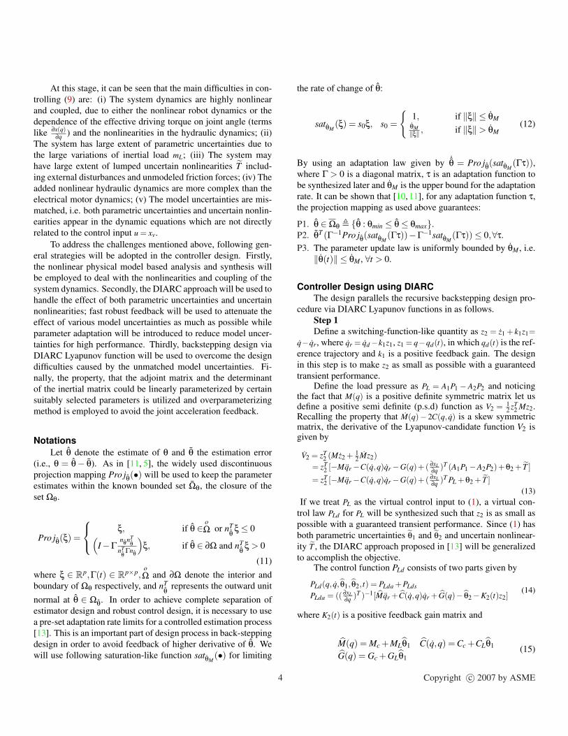
The system under consideration is depicted in Fig.1, whichrepresents a 3 DOF robot arm driven by three single-rod hy-draulic cylinders. The joint angles are represented by q =[q1,q2,q3]T . x = [xL1,xL2,xL3]T is the displacement vector of thehydraulic cylinders, which is uniquely related to the angle q, i.e.,xL1(q1), xL2(q2) and so on. The goal is to have joint angles q trackany feasible desired motion trajectories as closely as possible forprecision maneuver of the inertia load of the hydraulic robot arm.The rigid-body dynamics of the hydraulic arm can be describedby:

M(q)q+C(q, q)q+G(q) =(

∂x∂q

)T(A1P1−A2P2)+T (t,q, q) (1)

where P1 = [P11,P12,P13]T and P1i (i = 1,2,3) is the forward cham-ber pressures for the ith cylinder. P2 = [P21,P22,P23]T and P2i

Copyright c© 2007 by ASME

(i = 1,2,3) is the return chamber pressure of the ith cylinder.A1 = diag[A11,A12,A13] and A2 = diag[A21,A22,A23] are the ram ar-eas of the two chambers of the driving cylinders and T (t,q, q)∈R3

represents the lumped disturbance torque including external dis-turbances and terms like the friction torque.

Let mL be the unknown payload mounted at the end of the3rd arm, which is treated as a point mass for simplicity. Then, theinertial matrix M(q), coriolis terms C(q, q) and gravity terms G(q)in (1) can be linearly parametrized with respect to the unknownmass mL as

M(q) = Mc(q)+ML(q)mL,G(q) = Gc(q)+GL(q)mLC(q, q) = Cc(q, q)+CL(q, q)mL

(2)

where Mc(q), ML(q), Cc(q, q), CL(q, q), Gc(q), GL(q) are knownnonlinear functions of q and q. One of the properties of the inertiamatrix M(q) is that its inverse can be written as:

M−1(q) = M(q)/|M(q)| (3)

where |M(q)| represents the determinant of M(q), M(q) representsthe adjoint matrix of M(q). Furthermore, both M(q) and |M(q)|can be written as

|M(q)|= I = Ic +∑3i=1 Isimi

L M(q) = Mc +∑2i=1 Mimi

L (4)

where Ic, Isi, Mc and Mi are of the known functions of joint posi-tion q and I is a scalar.

Assuming no cylinder leakages, the actuator (or the cylin-der) dynamics can be written as,

V1(x)βe

P1 =−A1x+Q1 =−A1∂x∂q q+Q1

V2(x)βe

P2 = A2x−Q2 = A2∂x∂q q−Q2

(5)

where V1(x) = Vh1 + A1diag[x] ∈ R3×3 and V2(x) = Vh2 −A2diag[x]are the diagonal total control volume matrices of the twochambers of hydraulic cylinders respectively, which includethe hose volume between the two chambers and the valves,Vh1 = diag[Vh11,Vh12,Vh13] and Vh2 = diag[Vh21,Vh22,Vh23] are thecontrol volumes of the two chambers when x = 0, diag[x] =diag[x1L,x2L,x3L] , βe ∈ R is the effective bulk modulus, Q1 =[Q11,Q12,Q13]T is the vector of the supplied flow rates to the for-ward chambers of the driving cylinders, and Q2 = [Q21,Q22,Q23]T

is the vector of the return flow rates from the return chambers ofthe cylinders.

Let xv = [xv1,xv2,xv3] denotes the spool displacements of thevalves in the hydraulic loops. Define the square roots of the pres-sure drops across the two ports of the first control valve as:

g31(P11,sign(xv1)) =√

Ps−P11 for xv1 ≥ 0√P11−Pr xv1 < 0

g41(P21,sign(xv1)) =√

P21−Pr for xv1 ≥ 0√Ps−P21 xv1 < 0

(6)

where Ps is the supply pressure of the pump, and Pr is the tankreference pressure. Similarly, let g3i and g4i be the square rootsof the pressure drops for the ith hydraulic loop. For simplicity of

notation, define the diagonal square root matrices of the pressuredrops as:

g3(P1,sign(xv)) = diag[g31(P11,sign(xv1)), . . . ,g33(P1n,sign(xv3))]g4(P2,sign(xv)) = diag[g41(P21,sign(xv1)), . . . ,g43(P2n,sign(xv3))]

(7)Then, Q1 and Q2 in (5) are related to the spool displacements ofthe valves xv by ,

Q1 = kq1g3(P1,sign(xv))xv ,Q2 = kq2g4(P2,sign(xv))xv (8)

where kq1 = diag[kq11, . . . ,kq13] and kq2 = diag[kq21, . . . ,kq23] are theconstant flow gain coefficients matrices of the forward and returnloops respectively.

Given the desired motion trajectory qd(t), the objective is tosynthesize a control input u = xv such that the output y = q tracksqd(t) as closely as possible in spite of various model uncertain-ties.

ADAPTIVE ROBUST CONTROLLER DESIGNDesign Model and Issues to be Addressed

In this paper, for simplicity, we consider the parametric un-certainties due to the unknown payload mL, and the nominalvalue of the lumped disturbance vector T , Tn only. Other para-metric ucnertainties can be dealt with in the same way if nec-essary. In order to use parameter adaptation to reduce para-metric uncertainties to improve performance, it is necessary tolinearly parametrize the system dynamics equation in terms ofa set of unknown parameters. To achieve this, define the un-known parameter set as θ = [θ1,θ21,θ22,θ23]T where θ1 = mL andθT

2 = [θ21,θ22,θ23]T = Tn. The system dynamic equations can thusbe linearly parametrized in terms of θ as

M(q)q+C(q, q)q+G(q) =(

∂x∂q

)T(A1P1−A2P2)

+θ2 + T (t,q, q), T = T (t,q, q)−Tn

P1 = βeV−11 (q)

[−A1

∂x∂q q+Q1(u,g3(P1,sign(u))

]

P2 = βeV−12 (q)

[A2

∂x∂q q−Q2(u,g4(P2,sign(u))

](9)

Since the extent of the parametric uncertainties and uncertainnonlinearities are normally known, the following practical as-sumption is made. The following practical assumptions are madeabout parametric uncertainties and uncertain nonlinearities:

Assumption 1. The unknown parameter vector θ is within aknown bounded convex set Ωθ. Without loss of generality, it isassumed that, ∀θ∈Ωθ,θimin ≤ θi ≤ θimax, i = 1,21,22,23, whereθimax and θimin are some known constant.

Assumption 2. The uncertain nonlinearity d(t) can bebounded by a known function δd(t)

d(t) ∈Ωd , d : ‖d‖ ≤ δd(t) (10)

3 Copyright c© 2007 by ASME

At this stage, it can be seen that the main difficulties in con-trolling (9) are: (i) The system dynamics are highly nonlinearand coupled, due to either the nonlinear robot dynamics or thedependence of the effective driving torque on joint angle (termslike ∂x(q)

∂q ) and the nonlinearities in the hydraulic dynamics; (ii)The system has large extent of parametric uncertainties due tothe large variations of inertial load mL; (iii) The system mayhave large extent of lumped uncertain nonlinearities T includ-ing external disturbances and unmodeled friction forces; (iv) Theadded nonlinear hydraulic dynamics are more complex than theelectrical motor dynamics; (v) The model uncertainties are mis-matched, i.e. both parametric uncertainties and uncertain nonlin-earities appear in the dynamic equations which are not directlyrelated to the control input u = xv.

To address the challenges mentioned above, following gen-eral strategies will be adopted in the controller design. Firstly,the nonlinear physical model based analysis and synthesis willbe employed to deal with the nonlinearities and coupling of thesystem dynamics. Secondly, the DIARC approach will be used tohandle the effect of both parametric uncertainties and uncertainnonlinearities; fast robust feedback will be used to attenuate theeffect of various model uncertainties as much as possible whileparameter adaptation will be introduced to reduce model uncer-tainties for high performance. Thirdly, backstepping design viaDIARC Lyapunov function will be used to overcome the designdifficulties caused by the unmatched model uncertainties. Fi-nally, the property, that the adjoint matrix and the determinantof the inertial matrix could be linearly parameterized by certainsuitably selected parameters is utilized and overparameterizingmethod is employed to avoid the joint acceleration feedback.

NotationsLet θ denote the estimate of θ and θ the estimation error

(i.e., θ = θ− θ). As in [11, 5], the widely used discontinuousprojection mapping Pro jθ(•) will be used to keep the parameterestimates within the known bounded set Ωθ, the closure of theset Ωθ.

Pro jθ(ξ) =

ξ, if θ ∈ oΩ or nT

θ ξ≤ 0(I−Γ

nθnTθ

nTθ

Γnθ

)ξ, if θ ∈ ∂Ω and nT

θ ξ > 0

(11)where ξ ∈ Rp,Γ(t) ∈ Rp×p,

oΩ and ∂Ω denote the interior and

boundary of Ωθ respectively, and nTθ represents the outward unit

normal at θ ∈ Ωθ. In order to achieve complete separation ofestimator design and robust control design, it is necessary to usea pre-set adaptation rate limits for a controlled estimation process[13]. This is an important part of design process in back-steppingdesign in order to avoid feedback of higher derivative of θ. Wewill use following saturation-like function satθM

(•) for limiting

4

the rate of change of θ:

satθM(ξ) = s0ξ, s0 =

1, if ‖ξ‖ ≤ θM

θM‖ξ‖ , if ‖ξ‖> θM

(12)

By using an adaptation law given by ˙θ = Pro jθ(satθM(Γτ)),

where Γ > 0 is a diagonal matrix, τ is an adaptation function tobe synthesized later and θM is the upper bound for the adaptationrate. It can be shown that [10, 11], for any adaptation function τ,the projection mapping as used above guarantees:

P1. θ ∈Ωθ , θ : θmin ≤ θ≤ θmax.P2. θT (Γ−1Pro jθ(satθM

(Γτ))−Γ−1satθM(Γτ))≤ 0,∀τ.

P3. The parameter update law is uniformly bounded by θM , i.e.‖θ(t)‖ ≤ θM , ∀t > 0.

Controller Design using DIARCThe design parallels the recursive backstepping design pro-

cedure via DIARC Lyapunov functions in as follows.Step 1Define a switching-function-like quantity as z2 = z1 + k1z1=

q− qr, where qr = qd−k1z1, z1 = q−qd(t), in which qd(t) is the ref-erence trajectory and k1 is a positive feedback gain. The designin this step is to make z2 as small as possible with a guaranteedtransient performance.

Define the load pressure as PL = A1P1 − A2P2 and noticingthe fact that M(q) is a positive definite symmetric matrix let usdefine a positive semi definite (p.s.d) function as V2 = 1

2 zT2 Mz2.

Recalling the property that M(q)− 2C(q, q) is a skew symmetricmatrix, the derivative of the Lyapunov-candidate function V2 isgiven by

V2 = zT2 (Mz2 + 1

2 Mz2)= zT

2 [−Mqr−C(q,q)qr−G(q)+( ∂xL∂q )T (A1P1−A2P2)+θ2 + T ]

= zT2 [−Mqr−C(q,q)qr−G(q)+( ∂xL

∂q )T PL +θ2 + T ](13)

If we treat PL as the virtual control input to (1), a virtual con-trol law PLd for PL will be synthesized such that z2 is as small aspossible with a guaranteed transient performance. Since (1) hasboth parametric uncertainties θ1 and θ2 and uncertain nonlinear-ity T , the DIARC approach proposed in [13] will be generalizedto accomplish the objective.

The control function PLd consists of two parts given by

PLd(q, q, θ1, θ2, t) = PLda +PLds

PLda = (( ∂xL∂q )T )−1[Mqr +C(q,q)qr + G(q)− θ2−K2(t)z2]

(14)

where K2(t) is a positive feedback gain matrix and

M(q) = Mc +MLθ1 C(q,q) = Cc +CLθ1

G(q) = Gc +GLθ1(15)

Copyright c© 2007 by ASME

Substituting (14) into (13) and let z3 = PL−PLd represent the inputdiscrepancy, we will have

V2 = zT2 [( ∂xL

∂q )T PLds−φ2θ+ T ]− zT2 K2(t)z2 + zT

2 ( ∂xL∂q )T z3 (16)

whereφ2 = [−MLqr−CL(q,q)qr−GL(q), In×n] (17)

Then PLds and positive feedback gain matrix can be chosen tosatisfy:

condition i. zT2 [( ∂xL

∂q )T PLds−φ2θ+ T ]≤ ε2

condition ii. zT2 ( ∂xL

∂q )T PLds ≤ 0(18)

where ε2 is a design parameter which can be arbitrarily small. Es-sentially, first condition of (18) shows that PLds is synthesized todominate the model uncertainties coming from both parametricuncertainties θ and uncertain nonlinearities T , where as noninter-ference of robust part and adaptive part of the design is ensuredby second condiion. How to choose PLds to satisfy constraintslike (18) can be worked out in the same way as in [15] and [16].

Step 2In this step, an actual control law will be synthesized so

that z3 converges to designer-specified small value with a guar-anteed transient performance and accuracy. If we were to use thebackstepping design strategy via DIARC Lyapunov function asin [13], then, the resulting DIARC law would require the feed-back of the joint acceleration q , since q is needed in computingPLd , the calculable part of the derivative of the desired virtualcontrol function PLd , for adaptive model compensation. In or-der to avoid the need for joint acceleration feedback, in the fol-lowing, the property of the inertia matrix in (4) will be used asfollows.

Multiply both side of first equation of (9) by |M|M−1 = M wewill have

|M|q+MC(q,q)q+MG = M( ∂xL∂q )T PL +Mθ2 +MT (19)

DefineCt(q,q) = MC(q,q) Gt(q) = MGdn = Mθ2 d = MT

(20)

Thus (19) could be expressed by

Iq+Ct q+Gt = M( ∂xL∂q )T PL +dn + d (21)

where I is a scalar. Similar to (2), Ct , Gt and dn can be expressedby

Ct(q,q) = Ctc +∑ni=1 Ctiθi

1 Gt(q) = Gtc +∑ni=1 Gtiθi

1dn = Mcθ2 +∑n−1

i=1 Miθi1θ2

(22)

where Ctc and Gtc are of the known nonlinear functions of q andq.

From (22), redefine the unknown parameters as:

[β1,β2, · · · ,βn,βTn+1,β

Tn+2, · · · ,βT

2n]= [θ1,θ2

1, · · · ,θn1,θ

T2 ,θ1θT

2 , · · · ,θn−11 θT

2 ](23)

5

From (9), the derivative of z3 is given by

z3 = PL− PLd

PL = βe[−(A21V−1

1 +A22V−1

2 )( ∂xL∂q )T q+(A1V−1

1 Q1 +A2V−12 Q2)]

PLd = ∂PLd∂q q+ ∂PLd

∂q q+ ∂PLd

∂θ˙θ+ ∂PLd

∂t(24)

Define a p.s.d function as V3 = V2 + 12 IzT

3 z3. The derivative of V3is given by

V3 = V2|z3=0 + zT2 ( ∂xL

∂q )T z3 + IzT3 z3 + 1

2 IzT3 z3

= V2|z3=0 + zT3 (( ∂xL

∂q )T z2 + IPL− IPLd + 12 Iz3)

(25)

where V2|z3=0 represents the derivative of V2 when z3 = 0 and IPLdcan be expressed by

IPLd = IPLd + IPLd (26)

where

IPLd = ∂PLd∂q Iq+ ∂PLd

∂q (−Ct q− Gt + M( ∂xL∂q )T PL + dn)+ ∂PLd

∂t I + ∂PLd

∂θI ˙θ

IPLd = ( ∂PLd∂q q+ ∂PLd

∂θ˙θ+ ∂PLd

∂t )(−∑ni=1 Isiβi)

+ ∂PLd∂q [∑n

i=1(Ctiq+Gti)βi−∑n−1i=1 Mi( ∂xL

∂q )T PLβi−Mcβn+1

−∑ni=2 Mi−1βn+i + d]

I = Ic +∑ni=1 Isiβi, Ct = Ctc +∑n

i=1 Ctiβi

Gt = Gtc +∑ni=1 Gtiβi, dn = Mcβn+1 +∑n

i=2 Mi−1βn+i

M = Mc +∑n−1i=1 Miβi

(27)IPLd represents the calculable part of IPLd and will be used in

the model compensation part of the ARC control law in this step,IPLd is the incalculable part of IPLd and will be attenuated bycertain robust feedback.

Define

QL = A1V−11 Q1 +A2V−1

2 Q2 (28)

From (25), QL can be treated as the virtual control input in thisstep and we will synthesize an ARC control function QLd for QLsuch that PL will track the desired control virtual control inputPLd with a guaranteed transient and final tracking performance.Similar to the first step, QL is given by

QLd = QLda +QLds

QLda = (A21V−1

1 +A22V−1

2 )( ∂xL∂q )T q

+ 1Iβe

(−( ∂xL∂q )T z2 + IPLd − 1

2Iz3− IcK3z3)

(29)

where I = Ic +∑ni=1 Isiβi and K3 is a positive feedback gain matrix.

Substituting (29) in (25), we have

V3 = V2|z3=0 + zT3 (IβeQLds−φ3β+ ∂PLd

∂θI ˙θ− ∂PLd

∂q d)− zT3 IcK3z3 (30)

Copyright c© 2007 by ASME

where φ3 = [φ3(1), · · · ,φ3(n−1),φ3n,φ3(n+1),φ3(n+2), · · · ,φ3(2n)].

φ3(1) = Is1[βeQLda−βe(A21V−1

1 +A22V−1

2 )( ∂xL∂q )T q− ∂PLd

∂q q

− ∂PLd∂t ]+ ∂PLd

∂q (Ct1q+Gt1−M1( ∂xL∂q )T PL)+ 1

2 Is1z3

φ3(n−1) = Isn−1[βeQLda−βe(A21V−1

1 +A22V−1

2 )( ∂xL∂q )T q

− ∂PLd∂q q−− ∂PLd

∂t ]+ ∂PLd∂q (Ctn−1q+Gtn−1

−Mn−1( ∂xL∂q )T PL)+ 1

2 Isn−1z3

φ3n = Isn[βeQLda−βe(A21V−1

1 +A22V−1

2 )( ∂xL∂q )T q

− ∂PLd∂q q− ∂PLd

∂t ]+ ∂PLd∂q (Ctnq+Gtn)+ 1

2 Isnz3

φ3(n+1) =− ∂PLd∂q Mc

φ3(n+2) =− ∂PLd∂q M1

φ3(2n) =− ∂PLd∂q Mn−1

(31)

Thus QLds could be chosen to satisfy:

condition i. zT3 (IβeQLds−φ3β− ∂PLd

∂q d)≤ ε3

condition ii. zT3 (IβeQLds)≤ 0

(32)

where ε3 is a positive design parameter.Once the control function QLd for QL is synthesized as given

by (29), the actual control input u can be backed out from thecontinuous one-to-one nonlinear load flow mapping (28) as fol-lows. Noting that the elements of the diagonal matrices g3, g4,V1, and V2 are all positive functions, ui, the control input for theith hydraulic loop, should have the same sign as QLdi. Thus

ui = [A1iV−11i kq1ig3i(P1i,sign(QLdi))

+A2iV−12i kq2ig4i(P2i,sign(QLdi))]−1QLdi i = 1,2, . . . ,n

(33)

PARAMETER ADAPTATIONWe intend to use least square algorithm for parameter iden-

tification of the system. As indicated earlier in order to stressmore on the design philosophy rather than the actual design pro-cess, we will assume the uncertainty only in the mass lifted bythe robotic arm. Another parameter to be identified is the dc-likecomponent of the disturbance coming out of uncertain nonlin-earity like term. Even though all the states are available for themeasurement, the unavailability of rate of change of states sug-gests design of a filter circuit as in [7]. The following describesthe robot dynamics without presence of any uncertain nonlinear-ity

(Mm +θ1Mp)q+(Cm +θ1Cp)q+Bq+(Gm +θ1Gp)= ( ∂xL

∂q )T (P1A1−P2A2)+θ2(34)

Let H f (s) = 1τs+1 ,τ > 0 be a first order low-pass filter. Let Ω1 =

H f (Mm(q)q)) and Ω2 = H f (Mp(q)q). But, one important thingis to notice that as q is not available for measurement, we can’timplement this filter circuit directly.

6

Definition 1 (Filters Design for Parameter Adaptation).Let H f (s) = 1

τs+1 be a first order stable filter and let the filteredsignals be

ΩCm = H f [Cm(q, q)q],ΩCp = H f [Cp(q, q)q],ΩGm = H f [Gm(q)],ΩGp = H f [Gp(q)]ΩT = H f [( ∂xL

∂q )T (P1A1−P2A2)]

τΩ11 =−Ω11− 1τ Mm(q)q− Mm(q)q

Ω1 = Ω11 + 1τ Mm(q)q

τΩ2 =−Ω22− 1τ Mp(q)q− Mp(q)q

Ω2 = Ω22 + 1τ Mp(q)q

(35)

Now, we can write the robot dynamics as

y = Ω1 +ΩCm +ΩGm −ΩT = θ2−θ1[Ω2 +ΩCp +ΩGp ] (36)

Denoting Ψ(t)T = [−(Ω2 + ΩCp + ΩGp), I3×3] and θ =[θ1,θ21,θ22,θ23], we can write y = Ψ(t)T θ.

We implement the covariance-resetting, exponential-forgetting,recursive LSE [1] to regressor equation (36) to estimate θ:

Definition 2 (LSE Parameter Adaptation Algorithm).

˙θ(t) = Pro jθ(satθM(Γτ)), θ(0) ∈Ωθ

Γ(t) =

αΓ(t)− Γ(t)ΨΨT Γ(t)1+νtr(ΨΓΨT ) , if λmax(Γ(t))≤ ρM and

‖Pro jθ(Γτ)‖ ≤ θM

0 otherwise(37)

where τ = y−ΨT θ1+νtr(ΨΓΨT ) ,Γ(0) = ΓT (0) > 0,Γ(t+r ) = ρoI,ν ≥ 0.

In (37), α > 0 is the forgetting factor, tr is the covariance re-setting time, i.e., the time when λmin(Γ(t)) = ρ1 where ρ1 is thepre-set lower limit for Γ(t) satisfying 0 < ρ1 < ρ0. By limitingλmax(Γ(t)) ≤ ρM , we avoid the estimator wind-up when the re-gressor is not persistently exciting.

Main Theoretical ResultsLemma 1. When the rate-limited projection type adaptationlaw (37) is used, the following results hold:

θ ∈ L∞[0,∞), ΨT θ ∈ L∞[0,∞), ˙θ ∈ L∞[0,∞) (38)

In presence of no nonlinear uncertainties following additionalfacts also hold:

ΨT θ ∈ L2[0,∞), ˙θ ∈ L2[0,∞) (39)

Copyright c© 2007 by ASME

Proof: The boundedness of θ and ˙θ are guaranteed by projec-tion and saturated operator respectively. H f (s) is a stable filterand the regressor Ψ(t) is uniformly bounded. By choosing a pdfVθ = θT Γ−1θ, we can prove that Vθ = −cθT ΨΨT θ and hence,integrating the inequality we get ΨT θ ∈ L2[0,∞). ¤

Theorem 1. Let the parameter estimates θ be updated by theadaptation law (37). If the control law (33) is applied, then

A. Transient Performance: The tracking errors, z2 and z3,are bounded. Furthermore, V3, an index for the bound of thetracking errors, is bound above by

V3(t) ≤ exp(−λV t)V3(0)+ εVλV

[1− exp(−λV t)] (40)

where λV = 2mink2,k3IcmaxkM ,IM , εV = ε2 + ε3, kM is the upper

bound of the inertial matrix (i.e., M(q) ≤ kMI3×3 ), IM isthe upper bound of the determinant of inertial matrix, andk2 = inft>0 λmin(K2(t)),k3 = λmin(K3).

B. Asymptotic Tracking: After a finite time t0 ≥ 0, ifT (t+0 ) = 0, i.e., in the presence of parametric uncertaintiesonly, in addition to results in A, asymptotic output trackingis also obtained. 4

The derivative of V3 could be expressed by

V3 = zT2 (( ∂xL

∂q )T PLds−φ2θ+ T )+ zT3 (IβeQLds− ∂PLd

∂θI ˙θ−φ3β

− ∂PLd∂q d)− zT

2 Mz2− zT3 IcK3z3

(41)From the stabilizing condition of (18), (41) can be rewritten as

V3 ≤−zT2 Mz2− zT

3 IcK3z3 + ε2 + ε3≤−λVV3 + εV

(42)

which will lead to Part A by using Comparison Lemma [6]. ¤The proof of part B for general SISO nonlinear systems in semi-strict feedback forms can be found in [14].

Theorem 2 (Parametric Convergence). In the presence ofparametric uncertainties only, i.e. d = 0, by using control law(33) with rate limited projection type adaptation law (37), if thefollowing persistent excitation condition is satisfied:

∫ t+T

tΨ(τ)ΨT (τ)dτ≥ κpIp, for some κp > 0,T > 0 (43)

then the parameter estimates θ converge to their true values.( i.e., θ→ 0 as t → ∞.) 4Proof: From Lemma 1, ΨT θ is bounded and from (36), it iscontinuous; hence, it is uniformly continuous. Using Barbalat’sLemma, ΨT θ → 0 as t → 0. Following standard techniques inadaptive control [5], it is easy to show that 43 guarantees expo-nential convergence of parameters to its true value. ¤.

7

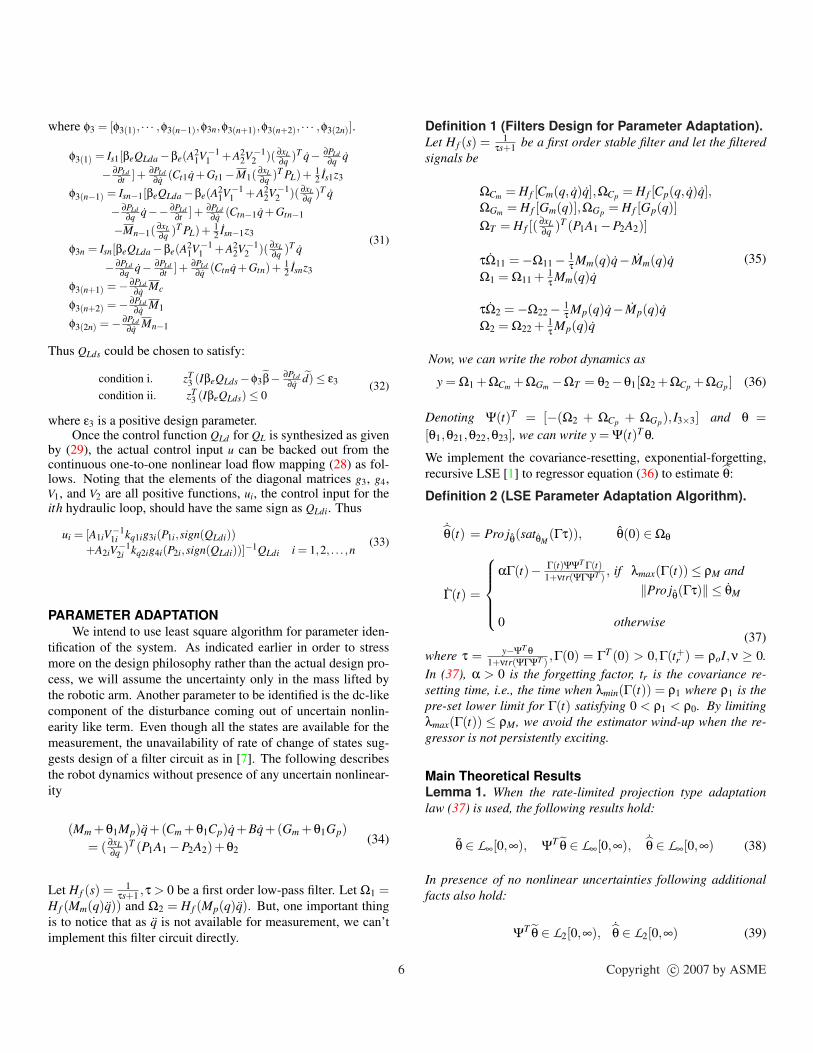
SIMULATION RESULTSExtensive simulations were carried out to check the valid-

ity of the proposed nonlinear integrated direct/indirect adaptiverobust algorithm under two scenarios. Firstly we considered asystem with constant disturbances and tried to estimate the massand disturbances of the system. In the second scenario Gaussiandisturbances with nonzero mean and a positive variance were es-timated along with unknown mass. The simulation model repre-sents a three-link robot arm (a scaled down version of industrialbackhoe loader arm) driven by three single-rod hydraulic cylin-ders as shown in Fig.1. The three hydraulic cylinders are con-trolled by two proportional directional control valves and oneservovalve manufactured by Parker Hannifan company. The dif-ferent arms are called swing, boom and stick.

The exact model of the hydraulic arm shown in Fig.1is quite messy and can be obtained from the authors. Pa-rameters of the actual arm used in the simulations are:m1 =22.98kg, m2 =24.94kg, m3 =19.68kg, mL = 20kg, l1 =0.3683m,l2= 0.9906m, and l3 =0.8001m. Hydraulic cylinder pa-rameters are: A1 =diag[2.0268 × 10−3,2.0268 × 10−3,2.0268 ×10−3]m2, A2 =diag[1.0688× 10−3,1.0688× 10−3,1.0688× 10−3]m2,Vh1 =diag[4.9953 × 10−4,5.2125 × 10−4,4.8505 × 10−4]m3, andVh2 =diag[9.0676×10−4,8.7237×10−4,9.2667×10−4]m3. The valveparameters are kq1 =diag[3.5904 × 10−8,3.5904 × 10−8,3.5904 ×10−8] m3

sec√

PaVand kq2 =diag[3.7206× 10−8,3.7206× 10−8,3.7206×

10−8] m3

sec√

PaV. The supplied pressure is Ps = 6.9× 106Pa and ac-

tual bulk modulus is βe = 2.7148× 108Pa. The desired jointposition vector is obtained by passing a pulse input to a thirdorder stable filter. The control gain and gain matrices arechosen as k1 = diag[350,400,350], K2 = diag[250,450,320], K3 =diag[350,400,220]. Other controller design parameters are ε2 =1×104, ε3 = 1×105.

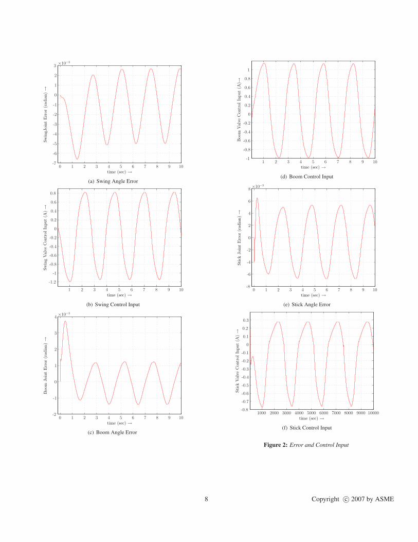
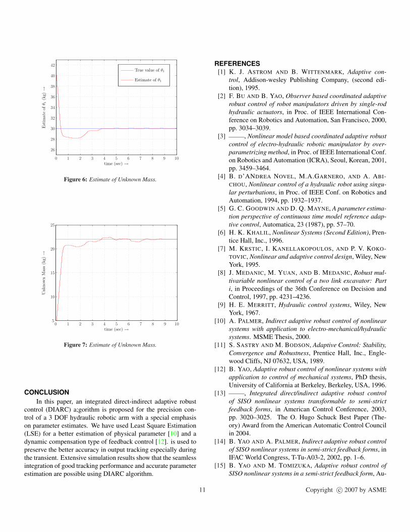
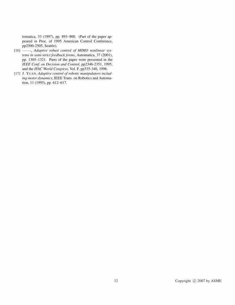
Constant Disturbances: The tracking errors of three jointsare shown in Fig.4(a), Fig.4(c) and Fig.4(e). As seen, the systemhas very small tracking errors during both transient period andsteady-state period. Fig. 4(b), Fig. 4(d) and Fig. 4(f) show thecontrol input of valves for three joints. The control inputs arewithin the control input saturation level ±10V . Fig. 7, Fig. 5(a),Fig. 5(b) and Fig. 5(c) show the least square estimates of thefour parameters as considered in the algorithm. The parameterestimates show very good convergence properties as comparedthe some of the previous result of using gradient law in [3], whilepreserving same tracking performance.

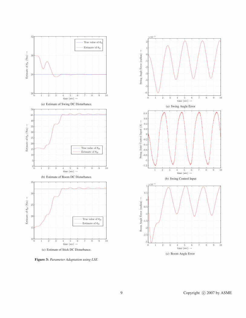
Disturbance with Nonzero Mean: The algorithm was alsoimplemented with nonzero mean bounded gaussian disturbancesand the seen in the results the nice properties of transient andsteady state performance are preserved. The system modelingimperfection due to disturbance degrades the parameter estima-tion process as expected. However, the overall performance ofthe estimation process as improved compared to gradient-typeestimation process.

Copyright c© 2007 by ASME

time (sec) →

Sw

ingJ

oint

Err

or(r

adia

n)→

0 1 2 3 4 5 6 7 8 9 10-7

-6

-5

-4

-3

-2

-1

0

1

2

3×10−3

(a) Swing Angle Error

time (sec) →

Sw

ing

Val

veC

ontr

olIn

put

(A)→

1 2 3 4 5 6 7 8 9 10

-1.2

-1

-0.8

-0.6

-0.4

-0.2

0

0.2

0.4

0.6

0.8

(b) Swing Control Input

time (sec) →

Boom

Joi

nt

Err

or(r

adia

n)→

0 1 2 3 4 5 6 7 8 9 10-2

-1

0

1

2

3

4×10−3

(c) Boom Angle Error

time (sec) →

Boom

Val

veC

ontr

olIn

put

(A)→

1 2 3 4 5 6 7 8 9 10-1

-0.8

-0.6

-0.4

-0.2

0

0.2

0.4

0.6

0.8

1

(d) Boom Control Input

time (sec) →

Sti

ckJoi

nt

Err

or(r

adia

n)→

0 1 2 3 4 5 6 7 8 9 10-8

-6

-4

-2

0

2

4

6

8×10−3

(e) Stick Angle Error

time (sec) →

Sti

ckV

alve

Con

trol

Input

(A)→

1000 2000 3000 4000 5000 6000 7000 8000 9000 10000-0.8

-0.7

-0.6

-0.5

-0.4

-0.3

-0.2

-0.1

0

0.1

0.2

0.3

(f) Stick Control Input

Figure 2: Error and Control Input

8 Copyright c© 2007 by ASME

time (sec) →

Est

imat

eof

θ21

(Nm

)→

True value of θ21

Estimate of θ21

0 1 2 3 4 5 6 7 8 9 1026

28

30

32

(a) Estimate of Swing DC Disturbance.

time (sec) →

Est

imat

eof

θ22

(Nm

)→

True value of θ22

Estimate of θ22

0 1 2 3 4 5 6 7 8 9 100

5

10

15

20

25

30

35

40

45

50

(b) Estimate of Boom DC Disturbance.

time (sec) →

Est

imat

eof

θ23

(Nm

)→

True value of θ23

Estimate of θ23

0 1 2 3 4 5 6 7 8 9 1010

15

20

25

30

35

(c) Estimate of Stick DC Disturbance.

Figure 3: Parameter Adaptation using LSE

time (sec) →

Sw

ing

Angl

eE

rror

(rad

ian)→

0 1 2 3 4 5 6 7 8 9 10

-6

-5

-4

-3

-2

-1

0

1

2

×10−3

(a) Swing Angle Error

time (sec) →

Sw

ing

Joi

nt

Con

trol

Input

(A)→

1 2 3 4 5 6 7 8 9 10

-1.2

-1

-0.8

-0.6

-0.4

-0.2

0

0.2

0.4

0.6

0.8

(b) Swing Control Input

time (sec) →

Boom

Angl

eE

rror

(rad

ian)→

0 1 2 3 4 5 6 7 8 9 10

-3

-2.5

-2

-1.5

-1

-0.5

0

0.5

1×10−3

(c) Boom Angle Error

9 Copyright c© 2007 by ASME

time (sec) →

Boom

Joi

nt

Con

trol

Input

(A)→

1 2 3 4 5 6 7 8 9 10

-1

-0.8

-0.6

-0.4

-0.2

0

0.2

0.4

0.6

0.8

1

(d) Boom Control Input

time (sec) →

Sti

ckA

ngl

eE

rror

(rad

ian)→

0 1 2 3 4 5 6 7 8 9 10-5

-4

-3

-2

-1

0

1

2

3

×10−3

(e) Stick Angle Error

time (sec) →

Sti

ckV

alve

Con

trol

Input

(A)→

1 2 3 4 5 6 7 8 9 10-0.8

-0.7

-0.6

-0.5

-0.4

-0.3

-0.2

-0.1

0

0.1

0.2

0.3

(f) Stick Control Input

Figure 4: Error and Control Input

time (sec) →

Est

imat

eof

θ21

(Nm

)→

0 1 2 3 4 5 6 7 8 9 1020

25

30

35

40

45

50

(a) Estimate of Swing DC Disturbance.

time (sec) →

Est

imat

eof

θ22

(Nm

)→

0 1 2 3 4 5 6 7 8 9 105

10

15

20

25

30

35

40

(b) Estimate of Boom DC Disturbance.

time (sec) →

Est

imat

eof

θ23

(Nm

)→

0 1 2 3 4 5 6 7 8 9 105

10

15

20

25

30

35

40

(c) Estimate of Stick DC Disturbance.

Figure 5: Parameter Adaptation using LSE

10 Copyright c© 2007 by ASME

time (sec) →

Est

imat

eof

θ1

(kg)

→

True value of θ1

Estimate of θ1

0 1 2 3 4 5 6 7 8 9 10

26

28

30

32

34

36

38

40

42

Figure 6: Estimate of Unknown Mass.

time (sec) →

Unknow

nM

ass

(kg)

→

0 1 2 3 4 5 6 7 8 9 105

10

15

20

25

Figure 7: Estimate of Unknown Mass.

CONCLUSIONIn this paper, an integrated direct-indirect adaptive robust

control (DIARC) a;gorithm is proposed for the precision con-trol of a 3 DOF hydraulic robotic arm with a special emphasison parameter estimates. We have used Least Square Estimation(LSE) for a better estimation of physical parameter [10] and adynamic compensation type of feedback control [12]. is used topreserve the better accuracy in output tracking especially duringthe transient. Extensive simulation results show that the seamlessintegration of good tracking performance and accurate parameterestimation are possible using DIARC algorithm.

1

REFERENCES[1] K. J. ASTROM AND B. WITTENMARK, Adaptive con-

trol, Addison-wesley Publishing Company, (second edi-tion), 1995.

[2] F. BU AND B. YAO, Observer based coordinated adaptiverobust control of robot manipulators driven by single-rodhydraulic actuators, in Proc. of IEEE International Con-ference on Robotics and Automation, San Francisco, 2000,pp. 3034–3039.

[3] , Nonlinear model based coordinated adaptive robustcontrol of electro-hydraulic robotic manipulator by over-parametrizing method, in Proc. of IEEE International Conf.on Robotics and Automation (ICRA), Seoul, Korean, 2001,pp. 3459–3464.

[4] B. D’ANDREA NOVEL, M.A.GARNERO, AND A. ABI-CHOU, Nonlinear control of a hydraulic robot using singu-lar perturbations, in Proc. of IEEE Conf. on Robotics andAutomation, 1994, pp. 1932–1937.

[5] G. C. GOODWIN AND D. Q. MAYNE, A parameter estima-tion perspective of continuous time model reference adap-tive control, Automatica, 23 (1987), pp. 57–70.

[6] H. K. KHALIL, Nonlinear Systems (Second Edition), Pren-tice Hall, Inc., 1996.

[7] M. KRSTIC, I. KANELLAKOPOULOS, AND P. V. KOKO-TOVIC, Nonlinear and adaptive control design, Wiley, NewYork, 1995.

[8] J. MEDANIC, M. YUAN, AND B. MEDANIC, Robust mul-tivariable nonlinear control of a two link excavator: Parti, in Proceedings of the 36th Conference on Decision andControl, 1997, pp. 4231–4236.

[9] H. E. MERRITT, Hydraulic control systems, Wiley, NewYork, 1967.

[10] A. PALMER, Indirect adaptive robust control of nonlinearsystems with application to electro-mechanical/hydraulicsystems. MSME Thesis, 2000.

[11] S. SASTRY AND M. BODSON, Adaptive Control: Stability,Convergence and Robustness, Prentice Hall, Inc., Engle-wood Cliffs, NJ 07632, USA, 1989.

[12] B. YAO, Adaptive robust control of nonlinear systems withapplication to control of mechanical systems, PhD thesis,University of California at Berkeley, Berkeley, USA, 1996.

[13] , Integrated direct/indirect adaptive robust controlof SISO nonlinear systems transformable to semi-strictfeedback forms, in American Control Conference, 2003,pp. 3020–3025. The O. Hugo Schuck Best Paper (The-ory) Award from the American Automatic Control Councilin 2004.

[14] B. YAO AND A. PALMER, Indirect adaptive robust controlof SISO nonlinear systems in semi-strict feedback forms, inIFAC World Congress, T-Tu-A03-2, 2002, pp. 1–6.

[15] B. YAO AND M. TOMIZUKA, Adaptive robust control ofSISO nonlinear systems in a semi-strict feedback form, Au-

1 Copyright c© 2007 by ASME

tomatica, 33 (1997), pp. 893–900. (Part of the paper ap-peared in Proc. of 1995 American Control Conference,pp2500-2505, Seattle).

[16] , Adaptive robust control of MIMO nonlinear sys-tems in semi-strict feedback forms, Automatica, 37 (2001),pp. 1305–1321. Parts of the paper were presented in theIEEE Conf. on Decision and Control, pp2346-2351, 1995,and the IFAC World Congress, Vol. F, pp335-340, 1996.

[17] J. YUAN, Adaptive control of robotic manipulators includ-ing motor dynamics, IEEE Trans. on Robotics and Automa-tion, 11 (1995), pp. 612–617.

12 Copyright c© 2007 by ASME