INTEGRALS 5. INTEGRALS We saw in Section 5.1 that a limit of the form arises when we compute an...
88
INTEGRALS INTEGRALS 5
-
date post
15-Jan-2016 -
Category
Documents
-
view
226 -
download
0
Transcript of INTEGRALS 5. INTEGRALS We saw in Section 5.1 that a limit of the form arises when we compute an...

INTEGRALSINTEGRALS
5

INTEGRALS
We saw in Section 5.1 that a limit of the form
arises when we compute an area.
We also saw that it arises when we try to find the distance traveled by an object.
1
1 2
lim ( *)
lim[ ( *) ( *) ... ( *) ]
n
in
i
nn
f x x
f x x f x x f x x
Equation 1

5.2The Definite Integral
In this section, we will learn about:
Integrals with limits that represent
a definite quantity.
INTEGRALS

DEFINITE INTEGRAL
If f is a function defined for a ≤ x ≤ b,
we divide the interval [a, b] into n subintervals
of equal width ∆x = (b – a)/n.
We let x0(= a), x1, x2, …, xn(= b) be the endpoints of these subintervals.
We let x1*, x2*,…., xn* be any sample points in these subintervals, so xi* lies in the i th subinterval.
Definition 2
DEFINITE INTEGRAL
Then, the definite integral of f from a to b is
provided that this limit exists.
If it does exist, we say f is integrable on [a, b].
1
( ) lim ( *)nb
ia ni
f x dx f x x
Definition 2

DEFINITE INTEGRAL
The precise meaning of the limit that
defines the integral is as follows:
For every number ε > 0 there is an integer N such that
for every integer n > N and for every choice of xi* in [xi-1, xi].
1
( ) ( *)nb
iai
f x dx f x x

INTEGRAL SIGN
The symbol ∫ was introduced by Leibniz
and is called an integral sign.
It is an elongated S.
It was chosen because an integral is a limit of sums.
Note 1

In the notation ,
f(x) is called the integrand.
a and b are called the limits of integration; a is the lower limit and b is the upper limit.
For now, the symbol dx has no meaning by itself; is all one symbol. The dx simply indicates
that the independent variable is x.
( )b
af x dx
( )b
af x dx
Note 1( )b
af x dxNOTATION

INTEGRATION
The procedure of
calculating an integral
is called integration.
Note 1

DEFINITE INTEGRAL
The definite integral is a number.
It does not depend on x.
In fact, we could use any letter in place of x
without changing the value of the integral:
( )b
af x dx
( ) ( ) ( )b b b
a a af x dx f t dt f r dr
Note 2( )b
af x dx
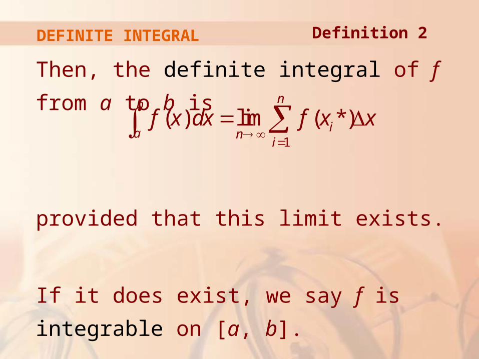
RIEMANN SUM
The sum
that occurs in Definition 2 is called
a Riemann sum.
It is named after the German mathematician Bernhard Riemann (1826–1866).
1
( *)n
ii
f x x
Note 3

RIEMANN SUM
So, Definition 2 says that the definite integral
of an integrable function can be approximated
to within any desired degree of accuracy by
a Riemann sum.
Note 3

RIEMANN SUM
We know that, if f happens to be positive,
the Riemann sum can be interpreted as:
A sum of areas of approximating rectangles
Note 3
Figure 5.2.1, p. 301

RIEMANN SUM
Comparing Definition 2 with the definition
of area in Section 5.1, we see that the definite
integral can be interpreted as:
The area under the curve y = f(x) from a to b
( )b
af x dx
Note 3
Figure 5.2.2, p. 301

RIEMANN SUM
If f takes on both positive and negative values, then the
Riemann sum is:
The sum of the areas of the rectangles that lie above the x-axis and the negatives of the areas of the rectangles that lie below the x-axis
That is, the areas of the gold rectangles minus the areas of the blue rectangles
Note 3
Figure 5.2.3, p. 301

RIEMANN SUM
When we take the limit of such
Riemann sums, we get the situation
illustrated here.
Note 3
© Thomson Higher Education
Figure 5.2.4, p. 301

NET AREA
A definite integral can be interpreted as
a net area, that is, a difference of areas:
A1 is the area of the region above the x-axis and below the graph of f.
A2 is the area ofthe region belowthe x-axis andabovethe graph of f.
1 2( )b
af x dx A A
Note 3
© Thomson Higher Education
Figure 5.2.4, p. 301

UNEQUAL SUBINTERVALS
Though we have defined by dividing
[a, b] into subintervals of equal width, there
are situations in which it is advantageous
to work with subintervals of unequal width.
In Exercise 14 in Section 5.1, NASA provided velocity data at times that were not equally spaced.
We were still able to estimate the distance traveled.
( )b
af x dx
Note 4

UNEQUAL SUBINTERVALS
If the subinterval widths are ∆x1, ∆x2, …, ∆xn,
we have to ensure that all these widths
approach 0 in the limiting process.
This happens if the largest width, max ∆xi , approaches 0.
Note 4

UNEQUAL SUBINTERVALS
Thus, in this case, the definition of
a definite integral becomes:
max 01
( ) lim ( *)i
nb
i ia xi
f x dx f x x
Note 4

INTEGRABLE FUNCTIONS
We have defined the definite integral
for an integrable function.
However, not all functions are integrable.
Note 5

INTEGRABLE FUNCTIONS
If f is continuous on [a, b], or if f has only
a finite number of jump discontinuities, then
f is integrable on [a, b].
That is, the definite integral exists.( )b
af x dx
Theorem 3

INTEGRABLE FUNCTIONS
To simplify the calculation of the integral,
we often take the sample points to be right
endpoints.
Then, xi* = xi and the definition of an integral simplifies as follows.

INTEGRABLE FUNCTIONS
If f is integrable on [a, b], then
where
1
( ) lim ( )i
nb
ia ni
f x dx f x x
and i
b ax x a i x
n
Theorem 4

DEFINITE INTEGRAL
Express
as an integral on the interval [0, π].
Comparing the given limit with the limit in Theorem 4, we see that they will be identical if we choose f(x) = x3 + x sin x.
3
1
lim ( sin )n
i i i in
i
x x x x
Example 1

DEFINITE INTEGRAL
We are given that a = 0 and b = π.
So, by Theorem 4, we have:
3 3
01
lim ( sin ) ( sin )n
i i i in
i
x x x x x x x dx
Example 1

DEFINITE INTEGRAL
In general, when we write
we replace: lim Σ by ∫ xi* by x
∆x by dx
1
lim ( *) ( )n b
i ani
f x x f x dx
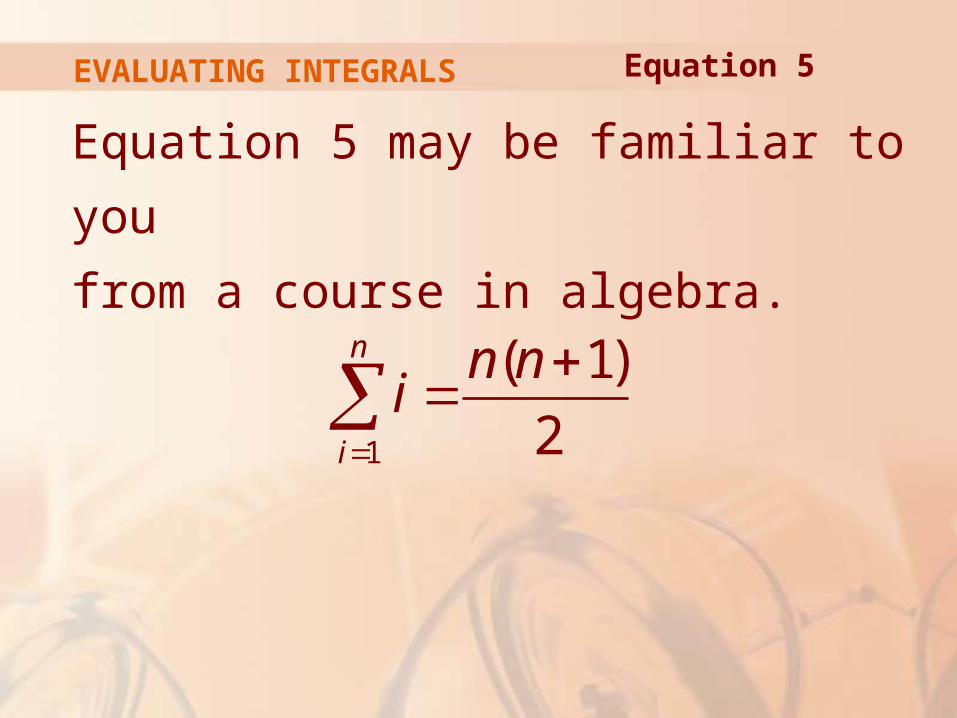
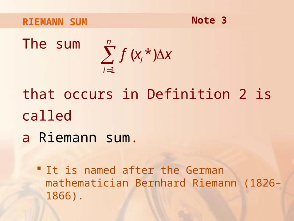
EVALUATING INTEGRALS
Equation 5 may be familiar to you
from a course in algebra.
1
( 1)
2
n
i
n ni
Equation 5

EVALUATING INTEGRALS
Equations 6 and 7 were discussed in
Section 5.1 and are proved in Appendix E.
2
1
( 1)(2 1)
6
n
i
n n ni
23
1
( 1)
2
n
i
n ni
Equations 6 & 7

EVALUATING INTEGRALS
The remaining formulas are simple rules for
working with sigma notation:
Eqns. 8, 9, 10 & 11
1
n
i
c nc
1 1
n n
i ii i
ca c a
1 1 1
( )n n n
i i i ii i i
a b a b
1 1 1
( )n n n
i i i ii i i
a b a b

EVALUATING INTEGRALS
a.Evaluate the Riemann sum for f(x) = x3 – 6x
taking the sample points to be right
endpoints and a = 0, b = 3, and n = 6.
b.Evaluate .3 3
0( 6 )x x dx
Example 2

EVALUATING INTEGRALS
With n = 6,
The interval width is:
The right endpoints are: x1 = 0.5, x2 = 1.0, x3 = 1.5, x4 = 2.0, x5 = 2.5, x6 = 3.0
3 0 1
6 2
b ax
n
Example 2 a

EVALUATING INTEGRALS
So, the Riemann sum is:6
61
12
( )
(0.5) (1.0) (1.5)
(2.0) (2.5) (3.0)
( 2.875 5 5.625 4 0.625 9)
3.9375
ii
R f x x
f x f x f x
f x f x f x
Example 2 a

EVALUATING INTEGRALS
Notice that f is not a positive function.
So, the Riemann sum does not
represent a sum of areas of rectangles.
Example 2 a

EVALUATING INTEGRALS
However, it does represent the sum of the areas of
the gold rectangles (above the x-axis) minus the
sum of the areas of the blue rectangles (below the
x-axis).
Example 2 a
Figure 5.2.5, p. 304

EVALUATING INTEGRALS
With n subintervals, we have:
Thus, x0 = 0, x1 = 3/n, x2 = 6/n, x3 = 9/n.
In general, xi = 3i/n.
3b ax
n n
Example 2 b

EVALUATING INTEGRALS3 3
0
1
1
3
1
33
1
( 6 )
lim ( )
3 3lim
3 3 3lim 6 (Eqn. 9 with 3/ )
3 27 18lim
n
ini
n
ni
n
ni
n
ni
x x dx
f x x
ifn n
i ic n
n n n
i in n n
Example 2 b

EVALUATING INTEGRALS Example 2 b
34 2
1 1
2
4 2
2
81 54lim (Eqns. 11 & 9)
81 ( 1) 54 ( 1)lim (Eqns. 7 & 5)
2 2
81 1 1lim 1 27 1
4
81 2727 6.75
4 4
n n
ni i
n
n
i in n
n n n n
n n
n n

EVALUATING INTEGRALS
This integral can’t be interpreted as
an area because f takes on both positive
and negative values.
Example 2 b

EVALUATING INTEGRALS
However, it can be interpreted as
the difference of areas A1 – A2, where
A1 and A2 are as shown.
Example 2 b
Figure 5.2.6, p. 304

EVALUATING INTEGRALS
This figure illustrates the calculation by showing the
positive and negative terms
in the right Riemann sum Rn for n = 40.
Example 2 b
Figure 5.2.7, p. 304

EVALUATING INTEGRALS
The values in the table
show the Riemann sums
approaching the exact
value of
the integral, -6.75,
as n → ∞.
Example 2 b
p. 304

EVALUATING INTEGRALS
a.Set up an expression for as
a limit of sums.
b.Use a computer algebra system (CAS)
to evaluate the expression.
5 4
2x dxExample 3

EVALUATING INTEGRALS
Here, we have f(x) = x4, a = 2, b = 5,
and
So, x0 = 2, x1 = 2 + 3/n, x2 = 2 + 6/n,
x3 = 2 + 9/n, and
xi = 2 + 3i / n
3
b ax
n n
Example 3 a
Figure 5.2.8, p. 305

EVALUATING INTEGRALS
From Theorem 4, we get:
5 4
21
1
4
1
lim ( )
3 3lim 2
3 3lim 2
n
in
i
n
ni
n
ni
x dx f x x
if
n n
i
n n
Example 3 a

EVALUATING INTEGRALS
If we ask a CAS to evaluate the sum
and simplify, we obtain:
4 3 2
31
3 2062 3045 1170 272
10
n
i
i n n n
n n
Example 3 b

EVALUATING INTEGRALS
Now, we ask the CAS to evaluate
the limit:
45 4
21
4 3 2
4
3 3lim 2
3 2062 3045 1170 27lim
103 2062 3093
618.610 5
n
ni
n
ix dx
n n
n n n
n
Example 3 b

EVALUATING INTEGRALS
Evaluate the following integrals by interpreting
each in terms of areas.
a.
b.
1 2
01 x dx
3
0( 1)x dx
Example 4

EVALUATING INTEGRALS
Since ,
we can interpret this integral as
the area under the curve
from 0 to 1.
Example 4 a
2( ) 1 0f x x
21y x

EVALUATING INTEGRALS
However, since y2 = 1
- x2, we get:
x2 + y2 = 1
This shows that the graph of f is the quarter-circle with radius 1.
Example 4 a
Figure 5.2.9, p. 305

EVALUATING INTEGRALS
Therefore,
In Section 8.3, we will be able to prove that the area of a circle of radius r is πr2.
1 2 2140
1 (1)4
x dx
Example 4 a
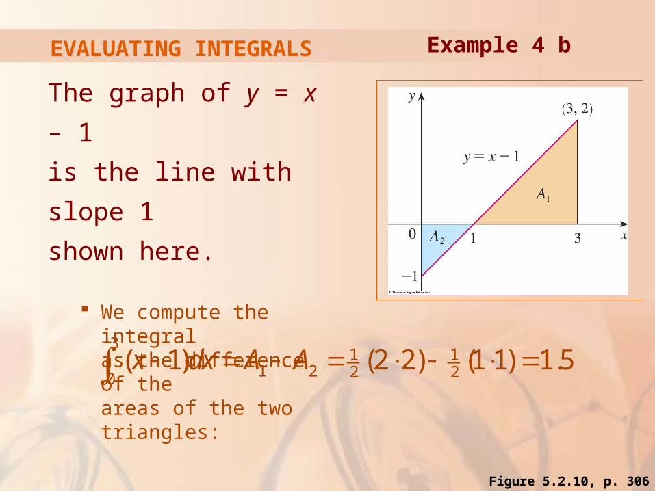
EVALUATING INTEGRALS
The graph of y = x – 1
is the line with slope 1
shown here.
We compute the integral as the difference of the areas of the two triangles:
31 1
1 2 2 20( 1) (2 2) (1 1) 1.5x dx A A
Example 4 b
Figure 5.2.10, p. 306

MIDPOINT RULE
However, if the purpose is to find
an approximation to an integral, it is usually
better to choose xi* to be the midpoint of
the interval.
We denote this by . ix

MIDPOINT RULE
Any Riemann sum is an approximation
to an integral.
However, if we use midpoints, we get
the following approximation.
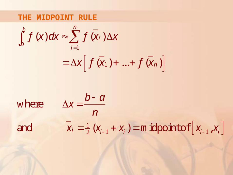
THE MIDPOINT RULE
1
1
11 12
( ) ( )
( ) ... ( )
where
and ( ) midpoint of ,
nb
ia
i
n
i i i i i
f x dx f x x
x f x f x
b ax
n
x x x x x

MIDPOINT RULE
Use the Midpoint Rule with n = 5
to approximate
The endpoints of the five subintervals are: 1, 1.2, 1.4, 1.6, 1.8, 2.0
So, the midpoints are: 1.1, 1.3, 1.5, 1.7, 1.9
2
1
1dxx
Example 5

MIDPOINT RULE
The width of the subintervals is: ∆x = (2 - 1)/5 = 1/5
So, the Midpoint Rule gives:
2
1
1(1.1) (1.3) (1.5) (1.7) (1.9)
1 1 1 1 1 1
5 1.1 1.3 1.5 1.7 1.9
0.691908
dx x f f f f fx
Example 5

MIDPOINT RULE
As f(x) = 1/x for 1 ≤ x ≤ 2, the integral
represents an area, and the approximation
given by the rule is the sum of the areas of
the rectangles shown.
Example 5
Figure 5.2.11, p. 306

MIDPOINT RULE
The approximation
M40 ≈ -6.7563
is much closer to
the true value -6.75 than
the right endpoint
approximation,
R40 ≈ -6.3998,
in the earlier figure.
Figure 5.2.12, p. 306
Figure 5.2.7, p. 304
PROPERTIES OF DEFINITE INTEGRAL
When we defined the definite integral
, we implicitly assumed that a < b.
However, the definition as a limit of Riemann
sums makes sense even if a > b.
( )b
af x dx

Notice that, if we reverse a and b, then ∆x
changes from (b – a)/n to (a – b)/n.
Therefore,
If a = b, then ∆x = 0, and so
( ) ( )a b
b af x dx f x dx
( ) 0a
bf x dx
PROPERTIES OF DEFINITE INTEGRAL

PROPERTIES OF THE INTEGRAL
We assume f and g are continuous functions.
1. ( ), where c is any constant
2. ( ) ( ) ( ) ( )
3. ( ) ( ) , where c is any constant
4. ( ) ( ) ( ) ( )
b
a
b b b
a a a
b b
a a
b b b
a a a
c dx c b a
f x g x dx f x dx g x dx
c f x dx c f x dx
f x g x dx f x dx g x dx

PROPERTY 1
Property 1 says that the integral of a constant
function f(x) = c is the constant times the
length of the interval.
( ), where c is any constantb
ac dx c b a

PROPERTY 1
If c > 0 and a < b, this
is to be expected,
because c(b – a) is the
area of the shaded
rectangle here.
Figure 5.2.13, p. 307

PROPERTY 2
Property 2 says that the integral of a sum
is the sum of the integrals.
( ) ( ) ( ) ( )b b b
a a af x g x dx f x dx g x dx
PROPERTY 2
For positive functions, it says that
the area under f + g is the area under
f plus the area under g.

PROPERTY 2
The figure helps us
understand why
this is true.
In view of how graphical
addition works, the corresponding vertical line segments have equal height.
Figure 5.2.14, p. 307

PROPERTY 2
In general, Property 2 follows from Theorem 4
and the fact that the limit of a sum is the sum
of the limits:
1
1 1
1 1
( ) ( ) lim ( ) ( )
lim ( ) ( )
lim ( ) lim ( )
( ) ( )
nb
i ia ni
n n
i ini i
n n
i in n
i i
b b
a a
f x g x dx f x g x x
f x x g x x
f x x g x x
f x dx g x dx

PROPERTY 3
Property 3 can be proved in a similar manner
and says that the integral of a constant times
a function is the constant times the integral
of the function.
That is, a constant (but only a constant) can be taken in front of an integral sign.
( ) ( ) , where c is any constantb b
a ac f x dx c f x dx

PROPERTY 4
Property 4 is proved by writing f – g = f + (-g)
and using Properties 2 and 3 with c = -1.
( ) ( ) ( ) ( )b b b
a a af x g x dx f x dx g x dx

PROPERTIES OF INTEGRALS
Use the properties of integrals to
evaluate
Using Properties 2 and 3 of integrals, we have:
1 2
0(4 3 )x dx
1 1 12 2
0 0 0
1 1 2
0 0
(4 3 ) 4 3
4 3
x dx dx x dx
dx x dx
Example 6

PROPERTIES OF INTEGRALS
We know from Property 1 that:
We found in Example 2 in Section 5.1 that:
1
04 4(1 0) 4dx
1 2 130
x dx
Example 6

PROPERTIES OF INTEGRALS
Thus,
1 1 12 2
0 0 0
13
(4 3 ) 4 3
4 3 5
x dx dx x dx
Example 6
PROPERTY 5
Property 5 tells us how to combine
integrals of the same function over
adjacent intervals:
( ) ( ) ( )c b b
a c af x dx f x dx f x dx

PROPERTY 5
However, for the case where f(x) ≥ 0 and
a < c < b, it can be seen from the geometric interpretation in
the figure.
The area under y = f(x) from a to c plus the area from c to b is equal to the total area from a to b.
Figure 5.2.15, p. 308

PROPERTIES OF INTEGRALS
If it is known that
find:
10 8
0 0( ) 17 and ( ) 12f x dx f x dx
Example 7
10
8( )f x dx

PROPERTIES OF INTEGRALS
By Property 5, we have:
So,
8 10 10
0 8 0( ) ( ) ( )f x dx f x dx f x dx
10 10 8
8 0 0( ) ( ) ( )
17 12
5
f x dx f x dx f x dx
Example 7

PROPERTIES OF INTEGRALS
Properties 1–5 are true
whether:a < ba = ba > b

COMPARISON PROPERTIES OF THE INTEGRAL
These properties, in which we compare sizes
of functions and sizes of integrals, are true
only if a ≤ b.
6. If ( ) 0 for , then ( ) 0
7. If ( ) ( ) for , then ( ) ( )
8. If ( ) for , then
( ) ( ) ( )
b
a
b b
a a
b
a
f x a x b f x dx
f x g x a x b f x dx g x dx
m f x M a x b
m b a f x dx M b a

PROPERTY 6
If f(x) ≥ 0, then represents
the area under the graph of f.
( )b
af x dx
If ( ) 0 for , then ( ) 0b
af x a x b f x dx

PROPERTY 7
Property 7 says that a bigger function has
a bigger integral.
It follows from Properties 6 and 4 because f - g ≥ 0.
If ( ) ( ) for ,
then ( ) ( )b b
a a
f x g x a x b
f x dx g x dx

PROPERTY 8
Property 8 is illustrated for the case where
f(x) ≥ 0. If ( ) for , then
( ) ( ) ( )
b
a
m f x M a x b
m b a f x dx M b a
Figure 5.2.16, p. 309

PROPERTY 8
If f is continuous, we could take m and M
to be the absolute minimum and maximum
values of f on the interval [a, b].
Figure 5.2.16, p. 309

PROPERTY 8
In this case, Property 8 says that:
The area under the graph of f is greater than the area of the rectangle with height m and lessthan the area of the rectangle with height M.
Figure 5.2.16, p. 309
PROPERTY 8—PROOF
Since m ≤ f(x) ≤ M, Property 7 gives:
Using Property 1 to evaluate the integrals
on the left and right sides, we obtain:
( )b b b
a a amdx f x dx M dx
( ) ( ) ( ) b
am b a f x dx M b a

PROPERTY 8
Use Property 8 to estimate
is an increasing function on [1, 4].
So, its absolute minimum on [1, 4] is m = f(1) = 1 and its absolute maximum on [1, 4] is M = f(4) = 2.
4
1 x dx
( ) f x x
Example 8

PROPERTY 8
Thus, by Property 8,
Example 8
4
1
4
1
1 4 1 2 4 1
or
3 6
x dx
x dx

PROPERTY 8
The result is illustrated here.
The area under from 1 to 4 is greater thanthe area of the lower rectangle andless than the area of the large rectangle.
y x
Example 8
Figure 5.2.17, p. 309