GEOPHYSICS, VOL. 13. NO. I (FEBRUARY IY78). P. 19-76, 37 FKS

INTEGRAL FORMULATION FOR MIGRATION IN TWO AND THREE DIMENSIONS

WILLIAM A. SCHNEIDER*

Computer migration of seismic data emerged in the late 1960s as a natural outgrowth of manual migration techniques based on wavefront charts and diffraction curves. Summation (integration) along a diffraction hyperbola was recognized as a way to automate the familiar point-to-point coordinate trans- formation performed by interpreters in mapping reflections from the x, t (traveltime) domain into the X, z (depth domain).

We will discuss the mathematical formulation of migration as a solution to the scalar wave equation in which surface seismic observations are the known boundary values. Solution of this boundary value problem follows standard techniques, and the mi- grated image is expressed as a surface integral over the known seismic observations when area1 or 3-D coverage exists. If only 2-D seismic coverage is available, wave equation migration is still possible by assuming the subsurface and hence surface re- corded data do not vary perpendicular to the seismic profile. With this assumption, the surface integral

reduces to a line integral over the seismic section, suitably modified to account for the implicit broad- side integral. Neither the 2-D or 3D integral migra- tion algorithms require any approximation to the scalar wave equation. The only limitations imposed are those of space and time sampling, and accurate knowledge of the velocity field.

Migration can also be viewed as a downward con- tinuation operation which transforms surface re- corded data to a deeper hypothetical recording surface. This transformation is convolutional in nature and the transfer functions tn both two and three dimensions are developed and discussed in terms of their characteristic properties Simple analy- tic and computer model data are migrated to illustrate the basic properties of migration and the fidelity of the integral method. Finally, applications of these algorithms to field data in both two and three dimen- sions are presented and discussed in terms of their impact on the seismic image.

INTRODUCTION

Migration of seismic data has been a basic tool of interpreters since at least the 1940s. The classic work of Hagedoom (1954) provided firm theoretical basis for the migration of time sections in two or three dimensions based upon the use of wavefront charts and diffraction curves. In the late 196Os, nu- merous computer implementations of Hagedoom’s migration principle became available for commercial use in seismic data processing. In the main, these programs accomplished migration by summation of stacked trace amplitudes along hyperbolic trajec- tories governed by the rms velocity distribution.

A recent revival in migration theory and practice stems principally from the work of Jon Claerbout (1970, 1972) and his colleagues at Stanford Uni- versity, who first formulated a finite-difference algorithm for migration based upon the scalar wave equation. Commercial programs at-c now available in industry to implement finite-difference migration of seismic data based on Claerbout’s original work and extensions thereof. These techniques are variously called “wave equation” migrations.

This paper develops an alternate view of wave equation migration in which the problem is posed as a boundary value problem, which leads naturally to

Presented at the 46th Annual International SEC Meeting, October 24, 1976 in Houston. Manuscript received by the Editor January 7, 1977; revised manuscript received June 26, 1977. *Formerly Texas Instruments, Dallas, TX.; currently Colorado School of Mines, Golden, CO 80401 0016-8033/78/0201-0049 $0X.00. @ 1978 Society of Exploration Geophysicists. All rights reserved.

49

Dow

nloa

ded

01/1

8/16

to 2

3.30

.65.

121.

Red

istr

ibut

ion

subj

ect t

o SE

G li

cens

e or

cop

yrig

ht; s

ee T

erm

s of

Use

at h

ttp://

libra

ry.s

eg.o

rg/

50 Schneider

an integral or summation algorithm for migration in either two or three dimensions. As will be seen, the integral solution has strong historic ties to the “con- ventional” diffraction summation approach of the late 1960s. The differences are subtle but significant ins turns of amplitude and waveform reconstruction. faithful to the scalar wave equation.

THEORY

For completeness, the integral migration algorithm will be derived from first principles starting with the scalar wave equation,

V’IJ ---& (In = -4rrq(r, t). FIG. 1. Geometry for boundary value solution.

The complete solution to the inhomogeneous wave equation in an arbitrary volume V, is given by a surface integral on S,, enclosing V, involving the boundary values, and a volume integral over I/, involving both source terms and initial values. This result is well known in the mathematical physics literature (see, for example, Morse and Feshback, 1953) and derives from an application of Green’s theorem. For our purposes, the volume integral may be ignored since the initial values are assumed to be zero before the shot instant, and there are no real sources in the subsurface image space, just reflectors and scatterers. Thus, we are left with the homoge- neous wave equation and inhomogeneous boundary conditions of the Dirichlet type. The remaining surface integral is given by,

U(r,1)=~Ilit,IdS,[G~U(r,,r,)

- U(r,, h) $-G 1 The specific geometry of interest is shown in Figure 1 with n the outward normal vector to the surface So. It includes the recording surface Z = 0 place, and a hemisphere extending to infinity in the subsurface. Contributions from the distant hemisphere are ig- nored, and the boundary value representation reduces to an integral over the surface involving the wave field on So and a suitable Green’s function G. Since U(r,, to) in equation (2) is equated to the observed seismic data, we require that G = 0 on So in order to eliminate the gradient of U, which may not also be independently specified, nor is it measured in current seismic practice. A Green’s function having the desired properties at the free surface consists of a point source at r0 and its negative image at rh, or

G(r, tl ro, to) = S(r-r,-;) *(r-ro-g

_ R R' ’

(3)

where

R = d(z - zo)* + (x - GI)~ + (Y - Yd2~

and

R’ = .\/(z + z# + (X - ~0)’ + (L’ - YI#.

Other choices of G are possible for image recon- struction purposes as discussed by Kuhn and Alhilali (1976). Substitution of equation (3) into equation (2) and simplification yields the following integral representation for the wave field U(r, t) at any point in image space in terms of observations of the wave field U(r,,, t,) on the surface,

dAo

This~ is a rigorous statement of Huygen’s principle and is commonly called the Kirchhoff integral. From the form of the kernel of equation (4), we recognize the transformation as a three-dimensional convolu- tion of the observed wave field w*ith a space-time operator related to the point source solution to the wave equation. We will return to this point subse- quently. Before doing so, however, it is instructive to re-express equation (4) by performing the indi- cated Z0 differentiation and t, integration resulting in an equivalent expression. D

ownl

oade

d 01

/18/

16 to

23.

30.6

5.12

1. R

edis

trib

utio

n su

bjec

t to

SEG

lice

nse

or c

opyr

ight

; see

Ter

ms

of U

se a

t http

://lib

rary

.seg

.org

/

Migration in Two and Three Dimensions 51

The bracketed term contains the time derivative of the recorded data plus the recorded data scaled by C/R or l/r the reciprocal traveltime, all evaluated at the ‘ ‘retarded’ ’ time to = 1 - R/C, Multiplying the brackets is the familiar “obliquity” factor. cos0. Because of the l/t multiplier, the second term in brackets is frequently dropped giving the Rayleigh-Sommerfeld diffraction formula of optics, Goodman (1968). However, it is no problem to re- tain both terms in seismic applications; we need only to differentiate the seismic section and add to it the same section scaled by l/t in order to implement equation (5) exactly. Trorey (1970), Hilterman (1970, 1975), and Berryhill (1976) make extensive use of the Kirchhoff integral [equation (S)] in forward modeling studies of diffraction and other propagation complexities in two and three dimensions. For a lucid discussion of the historic role of equation (5) and its many variants in optical, acoustic, and seismic imagery, the author recommends the excellent treat- ment given by Walter and Peterson (I 976).

Still another representation of equation (4) is pos- sible by interchanging the Z0 derivative with a Z derivative which may then be taken outside the in- tegral, giving

This is the most compact form and clearly demon- strates that the integral transformation is a solution to the 3-D wave equation by virtue of the form of the kernel f(t - R/C)/R. Now let us return to the convolutional aspects of this transformation. As noted previously, the integral transformation equa- tion (4) may be written symbolically as a three- dimensional convolution,

1 a [i )I 6 fk$

*-- 2n dzo

, (7) r

where

r2 = Az2 + x2 + J”.

which translates the observed wave field from one

q H (-lnzl)

H (IAzl)

MiGRATiOt-4 USES ii i+iAzlj TO EXTRAPOLATE CONVERGiNG ViNVES

FIG. 2. Extrapolation of converging and diverging waves. Dow

nloa

ded

01/1

8/16

to 2

3.30

.65.

121.

Red

istr

ibut

ion

subj

ect t

o SE

G li

cens

e or

cop

yrig

ht; s

ee T

erm

s of

Use

at h

ttp://

libra

ry.s

eg.o

rg/

52 Schneider

Z-plane to another. If we Fourier transform expres- sion (7) over X, y, and f (Appendix A), the operation becomes complex multiplication in the frequency wavenumber domain, giving

fi(k,, k,, z, w) = &k.r, k,, zo, QJ)

H(k,, k,, AZ, 4, (8)

where

to reflect the phase delay in propagation across the slab of thickness hZ. Conversely, we can make the clock run backward and compute the field at Z, from the field at Z2 by use of the positive sign in H

to reflect the phase advance in moving a distance AZ closer to the source. In the operation of migration we must use the positive sign in operator H to ex- trapolate converging waves back toward their ori- gins. With these basic mathematical tools to move data around, let us now review the principle of migration based on these integral transformations.

H = eZi, AZ, -k: - k-$. (9)

The transfer function H is seen to be a pure phase operator embodying the exact dispersion relation for the scalar wave equation. The operator H, expressed either in the space-time domain or frequency wave- number domain, enables us to extrapolate waves in space, which we will see shortly is basic to seismic image reconstruction. The choice of sign in equation (7) and (8) is important insofar as it determines the direction of extrapolation. To clarify the choice, consider Figure 2 which depicts a spherical wave radiating from S and two observation surfaces at Z, and Z2. The wave field at Z2 can be obtained from the field at Z,, which is closer to the source, by using expression (8) with the negative sign in operator H

(1) FIELD DATA - CDP STACK

G (x, y, o, t ) t

COINCIDENT SOURCE/RECEIVER

(2) Utx, y, o, t) = Glx, y, o, 2tl

ONE-WAY TIME

First, it is important to recognire that the wave field extrapolation equations developed thus far are not suitable for application to field records. While it is not difficult to pose the problem to accommodate shot-to-detector offset [see, for example, Timoshin (1970) and French (1975)], the mathematics are somewhat messier. For simplicity, we limit this discussion to the familiar CDP stack representation which approximates coincident source/receiver geometry as illustrated in Figure 3. Furthermore, the equations are cast in one-way traveltime so we can either divide our stacked section time scales by 2 or use a velocity in migration equal to l/2 the true velocity. With these two assumptions, it becomes clear that the “physical” experiment we are approx- imaging with stacked data is one in which the re-

Y G (x, y, o, t 1

s, r

FIG. 3. Migration principle: steps I and 2 Dow

nloa

ded

01/1

8/16

to 2

3.30

.65.

121.

Red

istr

ibut

ion

subj

ect t

o SE

G li

cens

e or

cop

yrig

ht; s

ee T

erm

s of

Use

at h

ttp://

libra

ry.s

eg.o

rg/

Migration-in TWS snd~ Jhree~ !limensians

(3) DOWNWARD EXTRAPOLATION

U (x, y, z, t ) = - &- 2 1’ dA

(4) IMAGING PRINCIPLE - EXTRAPOLATE RECEIVERS FOR ALL Z >O ATt = 0

u (x, y, z, 0) = - & + dxdy U(xl Y, o$ R

q 3D MIGRATION

FIG. 4. Migration principle: steps 3 and 4.

ceivers are located on the surface, the sources are positioned along the reflecting interfaces, their strengths are proportional to the reflection coeffi- cients, and they are fired in unison. That such a physical (though not necessarily practical) experi- ment could account for most if not all of the significant events present on a CDP stack section is of more than academic interest. Migration and other inverse wave equation processes require input data that are reasonably consistent with some forward propagation process. Not all current seismic processing tech- niques preserve the integrity of this forward-inverse re!ationship. For example, fast AGC applied either before or after stack can dramatically alter the ampli- tude of complex wave interferences which. if undis- turbed, can be unscrambled by migration in the inverse propagation process. Thus, given that the CDP stack, properly processed, is amenable to wave equation manipulation, we next insert this data into our previously derived transformation equation to downward extrapolate the surface recorded data to successively deeper levels, as depicted in Figure 4, step 3. This in itself is not yet migration, for the equation as written would give us a time function U(x, y, z, t) for each X, y, z position. Instead, we really only want to map a single value for each posi- tion, a value proportional to the reflection or scattering strength at that subsurface location, or in the context

of our “physical” experiment, we wish to map the equivalent source strength at all subsurface positions at the shot instant r = 0. Therefore, we must fix t = 0 and evaluate the integral for all X, y, z of interest as indicated in step 4 of Figure 4. This is 3-D migra-

tion for stacked data based on the Kirchhoff integral formula.

To further clarify this concept, consider Figure 5 which illustrates the input-output mapping relation- ship implied by the equations of Figure 4. The input assumes we have stacked data over the Z = 0 plane for the model shown. The output is a single trace at some .x, y !ocation plotted versus Z and vertical time Z/C. As the receiver moves down through SUC-

cessive positions, a point is mapped at each step by evaluating the integral with r = 0. For example, simulated receiver r1 at z1 maps a zero at t = 0 because the reflection has not arrived. Similarly, the response is zero at zz, and as becomes obvious, the integral will be zero when evaluated at zero travel- time unless the receiver is sitting on top of or very near the reflector. When it is, the reflection wavelet will be mapped at the vertical traveltime below the surface receiver position (actually below the CDP midpoint position). We recognize that this mapping procedure will produce the migrated picture.

Thus far, the development has assumed seismic observations are available over an area of sufficient D

ownl

oade

d 01

/18/

16 to

23.

30.6

5.12

1. R

edis

trib

utio

n su

bjec

t to

SEG

lice

nse

or c

opyr

ight

; see

Ter

ms

of U

se a

t http

://lib

rary

.seg

.org

/

Schneider

OUTPUT Ulx, y, z, 0)

_------z 0

.------- z 1

_-------z 2

,----___Z 3

---__-.z 4

_

--

--

_ -

_ -

t

Y

I//, INPUT utx, y, 0, t)

‘0-T *X

__________-_r,.-A__ __--- I

----__-_-- r _-•__--_

2 I

__----- i/

__-_r _ A _____ 3 I

/! ----- --‘47-----

Z

FIG. 5. Migration principle: input-output relationship.

extent to perform the indicated surface integrals or their discretized equivalents. This requires a 3-D seismic survey in which data are acquired over an entire prospect with space sampling of the order of one-half the shortest wavelengths of interest. While surveys of this kind have been and are now being conducted on a limited scale, the bulk of current seismic information is still 2-D, having been CO]- lected along widely spaced lines or traverses. In order to use the foregoing theory to migrate data from a single line and retain the benefits of a wave equation algorithm, we must make some assumption about the nature of the surface data U(x, y, 0, t) where we did not measure it. The most common practice is to assume the wave field at the surface is only 2-D; that is, if the line was shot in the x- direction, then

I/(x, .Y> 0, t) = U(x, 0, r),

independent of y. For this to be true, two conditions must be met: (I) the subsurface geology must be independent of _v, and (2) the source must either be a line source in the y-direction or the source and receiver must be colocated as is approximately the case in CDP stack. If these conditions are met, the appropriate 2-D transfer functions can be obtained

from equations (7) and (8), by either integrating out the y dependence in the 3-D space-time operator or setting k, = 0 in the frequency-vvave number oper- ator. The corresponding 2-D transfer functions are given below:

(10)

where

H = unit step function,

r= (z-zo)2+xZ,

and

H(&, AZ, w) = e’iiAzi \‘m. (11)

The resulting expressions (IO) and (I 1) are, of course, Fourier transform pairs and bear the same relationship to the 2-D wave equation solution as the 3-D transfer functions equations (7) and (8) bear to the 3-D wave equation. The 2-D migration algorithm obtained by convolving equation ( IO) with U(x, 0, r) and setting t = 0 as required by the mapping prin- ciple gives: D

ownl

oade

d 01

/18/

16 to

23.

30.6

5.12

1. R

edis

trib

utio

n su

bjec

t to

SEG

lice

nse

or c

opyr

ight

; see

Ter

ms

of U

se a

t http

://lib

rary

.seg

.org

/

Migration in Two and Three Dimensions 55

traces in this example is arbitrary, and generally is chosen to accommodate the maximum geologic timedip to be migrated. In principle, dips to 90 degrees and beyond can be migrated by the integral approach; however, this is not the case fol- finite-difference migration algorithms. Figure 7 shows a plot of an approximate 2-D transfer function obtained from equation (I 1) by assuming near vertical incidence propagation which yields

OFFSET (DEPTH POINTS)

FIG. 6. Exact 2-D transfer function.

This expression is somewhat more complicated looking than its 3-D counterpart of Figure 4, because

the y integral has been replaced by a time integral along the trace. In order to more fully appreciate the relationship between the 2-D and 3-D migration expressions, consider the following hypothetical experiment. First, consider migrating a seismic sec- tion using the 2-D expression given in equation ( 12). Next, imagine replicating that same input section many times to simulate shooting parallel lines in the dip direction of a 2-D subsurface model. Then 3-D migrate these parallel lines using the expression in Figure 4. The results of the two migrations will be identical; that is, expression (12) actually accom- plishes 3-D wave equation migration under the spe- cial circumstances that the surface recorded data are independent of one surface variable. When the above is not true, then equation (12) is not a valid migration, and as every interpreter should know, user beware!

Before leaving the mathematics of migration, it is instructive to examine the behavior of the 2-D trans- fer function, equation (IO), in more detail. Figure 6 shows a plot one-half the exact space-time operator as it would appear when being convolved with the section for an output value at 1 set vertical travel- time The operator shown is band-limited in both space and time appropriate to the sampling. The hyperbolic trajectory is predictable from simple ray theory considerations; however, the amplitude and phase behavior are not. The aperture width, ? 100

for

h-k,. C

This approximation is the basis of Claerbout’s (1972) so-called 1.5 degree finite difference algorithm. The approximate operator plotted in Figure 7 and the exact operator in Figure 6 are virtually identical near the apex corresponding to small dip angles. The ap- proximate operator decays more rapidly with offset and follows a parabolic rather than hyperbolic trajec- tory. Both these factors, plus frequency dispersion associated with finite differencing schemes, limit the accuracy and fidelity of finite difference migration in steeply dipping situations. While it is true that higher order approximations are possible and have been discussed by Claerbout (1976) and others. in the limit they can only approach the exact transfer function which the integral method achieves with ease. Next, let us examine the application of these migration algorithms to both model and field data.

MODEL RESULTS

First, consider the analytical migration of a plane

1.0

c

i!

S z

z

= 1.5

0 OFFSET (DEPTH POINTS)

FIG. 7. Approximate 2-D transfer function. Dow

nloa

ded

01/1

8/16

to 2

3.30

.65.

121.

Red

istr

ibut

ion

subj

ect t

o SE

G li

cens

e or

cop

yrig

ht; s

ee T

erm

s of

Use

at h

ttp://

libra

ry.s

eg.o

rg/

56 Schneider

Z 2

SURFACE DATA DOWNWARD CONTINUED DATA

Ulx, y, 0, t) = J$$ sin wt”

U(x, y, z.t) = wt”

z. case t’+ly _

C t”

x sine =1--T-- -

(z, - z) case

C

dt’ sine _I -- dx C

FIG. 8. Plane dipping reflector example.

dipping reflection depicted in Figure 8. On the left of the figure, we postulate a band-limited signal .S(t) emanating from a bed dipping at angle 0 in the X, z plane. The surface recorded data U(x, y. 0, t) is a delayed version of this signal, and the observed time dip dt ‘ldx is the familiar quantity sin 0/c. For this analytical signal we can actually analytically downward continue our receiver to a depth z using either equation (7) or (8). The result, U(X, y, z, t), is not unexpected and could have been arrived at by inspection. Since the receiver is a distance z closer to the reflector, the traveltime delay is reduced by z cos 0/c. Now to obtain the migrated time picture we must invoke the mapping principle by setting t = 0, and change variable from depth z to vertical time T = Z/C as shown by U(X, y, T, 0) in Figure 9. In migrated time space, the time dip dr’/dx after migration becomes tanB/c, and the bandwidth of the signal is reduced by cos0. Since migration is a loss-less process, the latter is purely a geometrical effect due to rotation of the reflection. Put another way, migration increases the time dip of a reflector by cos 0 and decreases the apparent signal frequency by the same factor so as to preserve horizontal wave- number.

Now let US examine the computeI’ migration of several simple synthetic sections. Figure 10 models four flat reflections and four dipping reflections with

time dips of 4, 8, 12, and 16 msec/trace, respec- tively. The reflection wavelet is a zero phase, O-80 Hz bandwidth pulse. A 2-D migrated picture is shown in Figure 11. A trace spacing of 25 m and velocity of 2500 misec were used resulting in struc- tural dips ranging from 12 to 53 degrees. The steepest event has migrated some 200 traces, or about 5 km.

f

-n

0

To = c

MIGRATED time PICTURE

Let: t - o, T- 5 - Vertical time

sincrl”7’ UN y.r, 0) = W’T’

T’ x tan0 ‘T- To - -

dT’ _x C 7F’ c

w’ * wcos.9

FIG. 9. Analytical migration of dipping reflector. Dow

nloa

ded

01/1

8/16

to 2

3.30

.65.

121.

Red

istr

ibut

ion

subj

ect t

o SE

G li

cens

e or

cop

yrig

ht; s

ee T

erm

s of

Use

at h

ttp://

libra

ry.s

eg.o

rg/

Migration in Two and Three Dimensions

4

FIG. 10. Synthetic time section modeling four flat reflections and four dipping reflections at 4, 8, 12, and 16 msecitr dip.

FIG. Il. 2-D migrated time section, AX = 25 m, V = 2500 misec.

The dots on the 53 degree event indicate the predicted yet these events are properly migrated including the migrated end points for the 16 msec/trace reflection aliased components. The question of migrating under in Figure 10, the correspondence is excellent. The sampled data is more complex than one might ex- slight tails on each of the migrated events result from pect, nor is it independent of the algorithm. With not including diffractions in the input model. The the integral approach it is possible to correctly mi- details of the result are more evident in Figures 12 grate aliased data by not spatially bandlimiting the and 13 which show enlarged portions of the input migration operator shown previously in Figure 6. section and migrated section, respectively. The low The risk in doing this is to generate migration back- level jitter on the input are sidelobes associated with ground noise which in the previous example is the sharp cutoffs in the wavelet design. The back- sufficiently low level to be unobjectionable. How- ground noise in the output is a combination of the ever, the effect is very sensitive to the space sampling above and migration noise. The expected results are AX. Figure 14 shows another ‘migration of the input also evident from these figures; namely, (I) the mi- model in Figure IO in which the trace interval was grated dip is greater than the unmigrated dip by cos doubled to 50 m; that is, the migration program was 8, and (2) the migrated pulse is reduced in apparent told the AX was 50 m instead of 25 m. but the identi- bandwidth by cos 8, thereby keeping the horizontal cal section was migrated. Of course, the implied wavenumber invariant. It is also interesting to note structural picture is different, and. as before, the the 12 and 16 msec/trace reflections have a signifi- events are correctly migrated, including aliased cant portion of their bandwidth beyond the l/2 wave- frequencies. The most notable difference, however, length Nyquist space sampling limit of 42 and 32 Hz, is the increase in migration noise from both flat and

FIG. 12. Detail of input section in Figure 10. FIG. 13. Detail of migrated section in Figure 11. Dow

nloa

ded

01/1

8/16

to 2

3.30

.65.

121.

Red

istr

ibut

ion

subj

ect t

o SE

G li

cens

e or

cop

yrig

ht; s

ee T

erm

s of

Use

at h

ttp://

libra

ry.s

eg.o

rg/

58 Schneider

‘\

\

:

FIG. 14. 2-D migrated time section, AX = 50 m, V = 2500 mlsec.

dipping events. This is basically a leakage problem caused by approximating the integral [equation (12)] by a discrete summation. The coarser the AX, the poorer the summation approximates the integral and the greater the leakage. While AX is a critical param- eter, the leakage also depends on frequency, velocity, migration aperture, and traveltime. In general, the leakage worsens with increasing AX, increasing frequency, increasing aperture, decreasing velocity, and decreasing traveltime. The problem also scales as the ratio of V/AX. In other words, the 50 m model with a 5000 m/set velocity would have the same low noise level as the 25 m, 2500 m/set migration in Figure Il. To guard against this problem on coarsely sampled data (whether or not it is aliased), the migration operator must be spatially bandlimited as in Figure 6 or, equivalently, a more sophisticated numerical integration must be used in lieu of discrete summation. Before leaving this sample plane dipping model, however, we will migrate it one more timeusing a AX of 16 m giving the result as shown in Figure 15. The third dipping event now appears as a greatly compressed 70 degree segment which has migrated some 300 traces horizontally and 1 .O to 1.5 set in time to its correct subsurface position. The missing fourth reflection does not represent a possible reflection in this model because its 16 msec/trace time dip exceeds the maximum of 13 msec/trace for a 90 degree reflector; hence it is not imaged.

As is apparent from these examples, the integral method has no algorithmic limitations on dip. Reflec- tions can be migrated to 90 degrees and beyond in the presence of vertical velocity gradients. The issues

FIG. 15. 2-D migrated time section, AX = 16 m, V = 2500 m/set.

of velocity and cost ultimately become the limiting factors, but before addressing the questions of veloc- ity inhomogeneity, another slightly more realistic model is of interest.

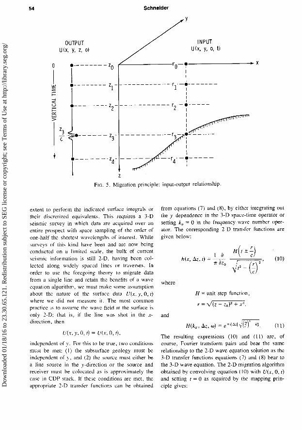
Figure 16 shows a synthetic zero offset timesection for three reflecting horizons of moderate complexity computed using a forward wave theory approach described by Trorey ( 1970). A constant 8000 ft/sec velocity was used, the trace interval is 50 ft, and the wavelet bandwidth is approximately O-60 Hz. Many of the classic diffraction phenomena so often seen on stacked sections are present. The 2-D integral migration shown in Figure 17 is virtually a perfect reconstruction of the subsurface acoustic impedance with accurate representation of the ampli- tude and waveform, structural attitude, curvature, and bed terminations. Were the world so simple, seismic processing would be a closed book. Un- fortunately, real seismograms are infinitely more complex than the constant velocity model depicted here, and much ptoggiess remains to be made in seismic processing techniques before we can accu- rately image in heterogeneous media.

Some of the more practical aspects of migrating seismic data are knowing what velocity to use, how to estimate it from the data, and how accurate it must be. None of these are trivial issues, nor shall I attempt to provide comprehensive answers. Certainly the issues of estimating seismic velocity for stacking and more recently for migration have received ample attention in the literature and in professional society meetings. I will not attempt to summarize the current art in this mature activity except to point out there is a trend away from CDP stack based vel- ocity analysis toward migration based techniques [Sattlegger (1975), Dohr (1975)]. The trend will undoubtedly accelerate as migration of unstacked

Dow

nloa

ded

01/1

8/16

to 2

3.30

.65.

121.

Red

istr

ibut

ion

subj

ect t

o SE

G li

cens

e or

cop

yrig

ht; s

ee T

erm

s of

Use

at h

ttp://

libra

ry.s

eg.o

rg/

Migration in Two and Three Dimensions 59

FIG. 16. Wave theory, zero offset time section modeled at 8000 ft/sec and 50 ft tract spacing.

data gradually replaces the CDP stack as the standard seismic image.

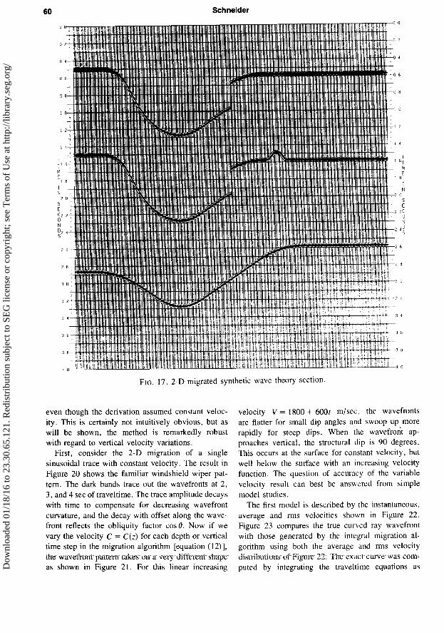
The question of (post stack) migration velocity sensitivity is somewhat more easily addressed, and I use the model in Figure 16 to illustrate the effects of slightly under and over migration. The section was remigrated with a velocity of 7600 ft/sec (5 percent low) and 8400 ft/sec (5 percent high). The results are shown in Figures 18 and 19, respectively. In a gross sense the pictures are very similar to Figure 17 migrated with the correct velocity. In

discernible, and, as expected, the flat reflections are totally insensitive to velocity. While not a com- prehensive answer to the velocity sensitivity ques- tion, we may readily conclude that: the more complex the subsurface, the more diffraction-like is the timesection, and the more accurate must the velocity be. Even with faulted simple geology, relatively small errors in migration velocity will improperly collapse the diffraction tails and blunt fault resolution.

VELOCITY INHOMOGENEITY

detail they differ; for example, the fault terminations In the foregoing development, starting with the are blurred, the flanks of the synclines are in error scalar wave equation and resulting in integral migra- by several hundred feet, and the small bump on the tion algorithms based thereon, it has been tacitly second reflector is severely distorted. Other distor- assumed the techniques could be successfully applied tions in amplitude and waveform are not readily to waves propagating in a variable velocity medium D

ownl

oade

d 01

/18/

16 to

23.

30.6

5.12

1. R

edis

trib

utio

n su

bjec

t to

SEG

lice

nse

or c

opyr

ight

; see

Ter

ms

of U

se a

t http

://lib

rary

.seg

.org

/

60 Schneider

FIG. 17. 2-D migrated synthetic wave theory section.

even though the derivation assumed constant veloc- ity. This is certainly not intuitively obvious, but as will be shown, the method is remarkedly robust with regard to vertical velocity variations.

First, consider the 2-D migration of a single sinusoidal trace with constant velocity. The result in Figure 20 shows the familiar windshield wiper pat- tern. The dark bands trace out the wavefronts at 2, 3, and 4 set of traveltime. The trace amplitude decays with time to compensate for decreasing wavefront curvature, and the decay with offset along the wave- front reflects the obliquity factor cos0. Now if we vary the velocity C = C(Z) for each depth or vertical time step in the migration algorithm [equation (12)], them wavefront- p~attern txkes on a very different~ shape as shown in Figure 21. For this linear increasing

velocity V = 1800 + tjOOt m/set, the wavefronts are flatter for small dip angles and swoop up more rapidly for steep dips. When the wavefront ap- proaches vertical, the structural dip is 90 degrees. This occurs at the surface for constant velocity, but well below the surface with an increasing velocity function. The question of accuracy of the variable velocity result can best be answered from simple model studies.

The first model is described by the instantaneous, average and rms velocities shown in Figure 22. Figure 23 compares the true curved ray wavefront with those generated by the integral migration al- gorithm using both the average and rms velocity distributions~ofFigure 22. The exuct curve -was com- puted by integrating the traveltime equations as D

ownl

oade

d 01

/18/

16 to

23.

30.6

5.12

1. R

edis

trib

utio

n su

bjec

t to

SEG

lice

nse

or c

opyr

ight

; see

Ter

ms

of U

se a

t http

://lib

rary

.seg

.org

/

Migration in Two and Three Dimensions 61

described by Musgrave (1961). For traveltimes of 1, 2, 3, and 4 set, the wavefronts are virtually iden- tical for dips less than 20 degrees. The rms velocity curve continues to track the exact wavefront to about 40 degrees and then departs gradually as the dip angle increases. Even out to approximately 60 de- grees the offset error is only about l-2 percent, which implies the velocity is too slow by the same amount.

A second model, Figure 24, presents a more com- plicated velocity distribution consisting of a deep water layer over a high-velocity subsurface. The wavefronts shown in Figure 25 tell a similar story; the ermrs are slightly greater due to the large dis- continuity at the water bottom, yet migration using

the rms velocity appears quite satisfactory to about 60 degrees, considering the expected accuracy of seismic velocity estimation.

A final model, Figures 26 and 27, shows a first order velocity discontinuity at depth between two linearly increasing functions. The errors are of the same magnitude as in the previous two models and suggests that for this class of linear increasing vel- ocity functions (with or without discontinuities), the strategy of using the vertical rms velocity in the integral migration algorithm [equation (12)] will produce quite accurate migrations to the order of 60 degrees structural dip. The errrors increase with angle and total distance traveled. At early times, less than 2 set for these models, accurate migrations

FIG. 18. Model in Figure 16 migrated at 7600 ftisec, 5 percent low velocity Dow

nloa

ded

01/1

8/16

to 2

3.30

.65.

121.

Red

istr

ibut

ion

subj

ect t

o SE

G li

cens

e or

cop

yrig

ht; s

ee T

erm

s of

Use

at h

ttp://

libra

ry.s

eg.o

rg/

62 Schneider

FIG. 19. Model in Figure 16 migrated at 8400 ftisec, 5 percent high velocity

can be obtained well beyond 60 degrees. Refine- ments are possible to improve accuracy at steeper dips by using ray-tracing strategies or modifying the rms velocity as a function of angle to approximate the rms velocity along the ray, which would give the exact result. At present, however, we do not believe these refinements are warranted until further ad- vances are made in estimating velocity with accuracy of the order of I percent in structurally complex geologic settings.

Horizontal velocity gradients present an additional complication to both migration and velocity estima- tion techniques. They can be “handled” from a mechanical point of view in much the same way as are the vertical gradients, by allowing the rms velocity term in the 2-D and 3-D migration algo-

rithms to vary with X, y, and Z. The errors in migra- tion caused by lateral velocity gradients are not as well understood as those caused by vertical gradients, and the matter is still being actively researched.

Let us now leave the theory and models and ex- amine several field examples of 2-D and 3-D migration.

FIELD EXAMPLES

The first 2-D migration example comes from the Gulf of Mexico. Figures 28 and 29 show, respec- tively, the stack section and migrated section. The trace interval is 50 m, typical Gulf velocities were used, and the display bandwidth is about 40 Hz shallow and 20 Hz at depth. Technically the result is very clean with virtually no migration noise or D

ownl

oade

d 01

/18/

16 to

23.

30.6

5.12

1. R

edis

trib

utio

n su

bjec

t to

SEG

lice

nse

or c

opyr

ight

; see

Ter

ms

of U

se a

t http

://lib

rary

.seg

.org

/

Migration in Two and Three Dimensions 63

-2

z ‘7ii E

-3

-4

-1

-2

1

E c

-3

-4

FIG. 20. Migrated 40 Hz sinewave at constant 2500 misec velocity.

FIG. 21. Migrated 40 Hz sinewave with varying velocity V = 1800 + 600 t misec.

artifacts, and waveform character has been well preserved. Geophysically, the main value of 2-D migration in this example is to enhance fault resolu- tion in the relatively simple sand/shale section. At depth, while some simplification occurs in the struc- tural picture, it would be remarkable if the assump- tions for valid 2-D migration were met; that is, sections parallel to this one would look exactly alike.

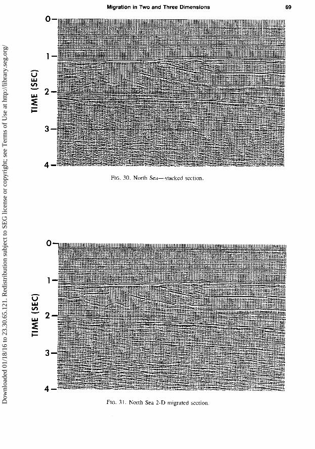
A second 2-D example comes from the North Sea. The CDP stack and 2-D migrated sections are shown in Figures 29 and 30, respectively. Trace spacing in this case is 25 m and the display band- width is higher than in the previous Gulf Coast ex- ample. The stacked section exhibits a simple Tertiary-Cretaceous section down to about 1 sec. Below the Cretaceous-Jurassic unconformity the data are complex, discontinuous, and exhibit numer- ous diffraction events. The 2-D migrated picture reveals a much more interpretable Jurassic section between 1 and 2 set, indicating major block faulting and tectonic activity probably related to salt move- ment. In particular, several small fault blocks on the left of the section and also just right of center are virtually obscured by diffractions on the stacked section. After migration, they stand out with remark- able clarity. as does the uncomformity at the base of the Cretaceous. Overall, the waveform and char- acter of the input section are faithfully preserved in the migrated picture, due principally to the wave equation formulation of the algorithm. This is per- haps the most significant difference between this “Kirchhoff” based migration and the earlier diffraction-summation techniques.

Whether the structural picture portrayed here by migration is correct cannot be answered from this result alone; additional seismic control is necessary. In general, from our experience we know complex geology is seldom sufficiently two-dimensional to satisfy the assumptions required for 2-D migration. While French (1975) extends the range of applica- bility of 2-D migration to both oblique profiles and plunging 2-D structures, there is no substitute for 3-D data and 3-D migration to correctly image seismic returns from complex geologic targets.

Until recently 3-D seismic data acquisition and processing were more of a research curiosity than a practical exploration tool. However, continuing advances in computer hardware and software coupled with innovations in seismic data acquisition over the

VELOCITY (KFT/SEC) 10 15. .20 25 30

1

FIG. 22. Velocity function-model 1. Dow

nloa

ded

01/1

8/16

to 2

3.30

.65.

121.

Red

istr

ibut

ion

subj

ect t

o SE

G li

cens

e or

cop

yrig

ht; s

ee T

erm

s of

Use

at h

ttp://

libra

ry.s

eg.o

rg/

64 Schneider

OFFSET IKFT)

FIG. 23. Wavefront

MIGRATION WAVEFRONT V, MIGRATION WAVEFRONT V,,,,,

EXACT WAVEFRONT

curves for model 1 showing the exact and approximate wavefronts using the average rms velocities in the Kirchhoff migration integral.

and

past several years now make it economically feasible to conduct 3-D surveys on both land and marine prospects. Tegland (1976) describes some of these significant advances which include streamer tracking systems to locate accurately the streamer relative to the boat for each shot, apd efficient land 3-D col- lection techniques based on crooked traverses and perimeter shooting. An example of the latter applied to a California land prospect is shown in Figure 32. The technique, called Seisloop/Seisquare’, obtains 3-D coverage by shooting around regular or irregular loops into geophones emplaced completely around the perimeter of the same loop. In this prospect, 14 rectangular loops covering IO sq mi were shot using Vibroseism source patterns at each of the large dots, into geophone arrays at each small dot. Each source- receiver midpoint location is calculated and the cor- responding trace assigned to a unique “bin” 330 ft square, resulting in the regular CDP map of Figure 33. Traces common to a bin are stacked together after static and NM0 corrections have been applied, yielding a set of stacked traces on a uniform 330 ft X, y grid with an average CDP fold of six. These data may be arranged for display in numerous ways, Figure 34 shows a north-south gather of CDP lines 19, 20, and 21 which are 330 ft apart and about 3 miles long. Data quality is fair to good in the shallow section. The geology is complex showing strong north dip, and well control indicates that the shallow

‘Service Mark of GSI. U.S. Patent No. 3,867,713. @Continental Oil Co.

gas production is controlled by numerous small fault blocks. The prospect is an old field with 25 existing wells, generally thought to be drilled out. 3-D seis- mic was tried in an attempt to uncover additional secondary fault traps in a mature field development situation. As a result of the 3-D survey, five new drilling locations were identified, and as of this writ- ing, two have been drilled and tested commercial gas with recoverable economic value about ten times the cost of the 3-D survey and drilling.

Of major significance in this project was the ap- plication of 3-D migration based on the formula of Figure 4 appropriately discretized for sampled data input. Figure 35 shows three output sections from the

VELOCITY (KFT/SEC)

FIG. 24. Velocity function-model 2. Dow

nloa

ded

01/1

8/16

to 2

3.30

.65.

121.

Red

istr

ibut

ion

subj

ect t

o SE

G li

cens

e or

cop

yrig

ht; s

ee T

erm

s of

Use

at h

ttp://

libra

ry.s

eg.o

rg/

Migration in Two and Three Dimensions

OFFSET (KFT)

65

b

MIGRATION WAVEFRONT V, MIGRATION WAVEFRONT V,,, EXACT WAVEFRONT

FIG. 25. Wavefront curves for model 2.

3-D migration process at the same locations as the CDP stack lines in Figure 34. Each trace in the mi- grated picture results from a weighted sum over a square aperture of 10 x 10 input CDP stacked traces. The aperture size was determined by the maximum time dip rates as seen on the stacked sections in the north-south direction and between lines in the east- west direction.

For comparison, Figure 36 shows the same three lines migrated with the 2-D algorithm. The clarity and definition of the 3-D migration are superior to both the 2-D migration and CDP stack at all levels. In fairness to the latter, however, it should be noted that 6-fold conventional shooting is not a very heavy field effort by current standards. Better conventional 2-D results could have been obtained with higher fold shooting. That more conventional seismic would have contributed to finding additional reserves in this field is questionable since several generations of 2-D work had already been exploited to their fullest in discovering the known reserves. The key to finding any remaining pools was dense spatial sampling and accurate location of small untested fault blocks, both of which the 3-D migrated data addressed. Of sec- ondary interest is a major unconformity seen at about I.5 set on the 3-D sections, but rather obscure on the CDP and 2-D migrated sections. This uncon- formity may play a significant role in deeper untested targets in the field. Its expression is more apparent on east-west lines illustrated in Figure 37, showing two 3-D migrated lines gathered across the prospect 660 ft apart. Also evident are numerous north-south

trending faults which control the shallow gas pro- duction.

Of considerable importance to the overall success of this project was the confidence placed in the 3-D migrated result by the geologist-interpreter because it tied subsurface well control, whereas the stacked sections did not. Finally, in retrospect, the 330 ft bin size was marginally adequate for the exploration objective in terms of structural dip and resolution implications. The space sampling intervals &, AY are critical parameters in 3-D surveys and must be selected to meet the geologic and resolution objec- tives within the economic constraints imposed on the program. In general, 3-D seismic surveys will,

vEtociTY (KFT/SEC)

FIG. 26. Velocity function- model 3. Dow

nloa

ded

01/1

8/16

to 2

3.30

.65.

121.

Red

istr

ibut

ion

subj

ect t

o SE

G li

cens

e or

cop

yrig

ht; s

ee T

erm

s of

Use

at h

ttp://

libra

ry.s

eg.o

rg/

because of their custom problem-solving nature, re- quire a much greater degree of prep~hmnirrg and client-contractor interplay than conventional seismic surveys.

SUMMARY AND CONCLUSIONS

Our understanding of migration has come a long way from the era of wavefront charts and curves of maximum convexity. We now view the operation as a rigorous inverse wave propagation process sub- ject only to the limitations of the scalar wave equation assumption. and our ability to estimate propagation velocity. Both these areas will undoubtedly be the focal points for further improvements in migration practice in the years ahead.

This discussion has centered on the integral formu- lation for migration. The finite-difference school also has its advocates and supporters and no attempt was made here to plead their case. Loewenthal (1974), Koehler (1976). Larner (1976), and others have dis- cussed the latter in considerable detail. To claim one approach is vastly superior to the other is to ignore the fact that both integral and tinite-difference migra- tions are based on the scalar wave equation. In the limit of no approximations in implementation they would yield the same results.

In the author’s opinion, the integral method offers the following advantages:

I) The 2-D and 3-D algorithms can be implemented without approximating the scalar wave equation.

Data can be migrated to 90 degrees and beyond, velocity accuracy and cost being the only real limitations. In 3-D applications, departure from a regular X, v grid can be easily accommodated by the integral method. This occurs frequently in both land and marine applications because of the difficulty in collecting seismic data exactly where you want it. Finally, the integral method lends itself more readily to ad hoc weighting schemes which are meant to combat seismic noise not comprehended by any of the current wave equation formulations for migration.

ACKNOWLEDGMEN’I’S

The author wishes to thank his colleagues, Cam Wason and Bruce Secrest, for their many helpful, theoretical discussions relevant to the concepts pre- sented herein. My thanks also go to Frank Linville, Chyi Lu, and Bob Hester for their sxsistance in pre- paring the model results. And, finally. the author is grateful to Texas Instruments for permission to pub- lish this work.

REFERENCES Berryhill, J. R.. 1976, Diffraction responsefor nonzero

separation of source and receiver: &physics, v. 42, P. 1158-1176.

Claerbout, Jon F., 1970, Coarse grid calculations of waves in inhomogeneous media with application to delineation of complicated seismic structure: Ceophqsics. v. 35, p. 407-418. (Text continued on p. 76)

OFFSET (KU)

FIG. 27. Wavefront curves for model 3.

MIGRATION WAVEFRONT V, MIGRATION WAVEFRONT V,,,

EXACT WAVEFRONT

Dow

nloa

ded

01/1

8/16

to 2

3.30

.65.

121.

Red

istr

ibut

ion

subj

ect t

o SE

G li

cens

e or

cop

yrig

ht; s

ee T

erm

s of

Use

at h

ttp://

libra

ry.s

eg.o

rg/

O-

1

2-

3-

4-

5-

Migration in Two and Three Dimensions 67

FIG. 28. Gulf of Mexico CDP stacked section. Dow

nloa

ded

01/1

8/16

to 2

3.30

.65.

121.

Red

istr

ibut

ion

subj

ect t

o SE

G li

cens

e or

cop

yrig

ht; s

ee T

erm

s of

Use

at h

ttp://

libra

ry.s

eg.o

rg/

Dow

nloa

ded

01/1

8/16

to 2

3.30

.65.

121.

Red

istr

ibut

ion

subj

ect t

o SE

G li

cens

e or

cop

yrig

ht; s

ee T

erm

s of

Use

at h

ttp://

libra

ry.s

eg.o

rg/

time (SEC)

P w IQ

n a w

time (SEC)

P Ia 0

Dow

nloa

ded

01/1

8/16

to 2

3.30

.65.

121.

Red

istr

ibut

ion

subj

ect t

o SE

G li

cens

e or

cop

yrig

ht; s

ee T

erm

s of

Use

at h

ttp://

libra

ry.s

eg.o

rg/

70 Schneider

FIG. 32. California land 3-D prospect map showing location of source and receiver positions.

Dow

nloa

ded

01/1

8/16

to 2

3.30

.65.

121.

Red

istr

ibut

ion

subj

ect t

o SE

G li

cens

e or

cop

yrig

ht; s

ee T

erm

s of

Use

at h

ttp://

libra

ry.s

eg.o

rg/

Migration in Two and Three Dimensions 71

FIG. 33. California land 3-D prospect map showing grid of CDP bin center locations.

Dow

nloa

ded

01/1

8/16

to 2

3.30

.65.

121.

Red

istr

ibut

ion

subj

ect t

o SE

G li

cens

e or

cop

yrig

ht; s

ee T

erm

s of

Use

at h

ttp://

libra

ry.s

eg.o

rg/

72 Schneider

time (SEC) 0 0 9 9 0

d r: cy m 4

Dow

nloa

ded

01/1

8/16

to 2

3.30

.65.

121.

Red

istr

ibut

ion

subj

ect t

o SE

G li

cens

e or

cop

yrig

ht; s

ee T

erm

s of

Use

at h

ttp://

libra

ry.s

eg.o

rg/

Migration in Two and Three Dimensions 73

time (SEC) 0 cy-

0 0 0

d C c\i c4 +

0 -

0 4

0 r:

0 d

0 ci

(33s) 3WIl

Dow

nloa

ded

01/1

8/16

to 2

3.30

.65.

121.

Red

istr

ibut

ion

subj

ect t

o SE

G li

cens

e or

cop

yrig

ht; s

ee T

erm

s of

Use

at h

ttp://

libra

ry.s

eg.o

rg/

74 Schneider

time (SEC) 9 9 0 0 0 0 cu’ ti +

Dow

nloa

ded

01/1

8/16

to 2

3.30

.65.

121.

Red

istr

ibut

ion

subj

ect t

o SE

G li

cens

e or

cop

yrig

ht; s

ee T

erm

s of

Use

at h

ttp://

libra

ry.s

eg.o

rg/

Migration in Two and Three Dimensions

DEPTH (KFT)

0 0 0 0 0 6 cu’ 4 4 od

0 0 0 0 6 cj i 4

9 0 0 0 d

“,l,,,_ cy 9 4 4

- - - WI)

time (SEC)

9 0 0 0 0

0 4 cu’ Pi i

0 6 0 0 0 0 4 Pi ci +

Dow

nloa

ded

01/1

8/16

to 2

3.30

.65.

121.

Red

istr

ibut

ion

subj

ect t

o SE

G li

cens

e or

cop

yrig

ht; s

ee T

erm

s of

Use

at h

ttp://

libra

ry.s

eg.o

rg/

- 1976, Fundamentals of geophysical data process- ing: New York, McGraw-Hill Book Co., Inc.

Claerbout, Jon F., and Doherty, S. M., 1972, Downward continuation of moveout corrected seismograms: Geo- physics, v. 37, p. 741-768.

Dohr, G. P.,, and Stiller, P: K., 1975; Migration vdoeity determination: Part 11. Applications: Geophysics, v. 40, p. 6-16.

French, W. S., 1975, Computer migration of oblique seis- mic reflection profiles: Geophysics, v. 40, p. 961-980.

Goodman, J. W., 1968, Introduction to Fourier optics: New York, McGraw-Hill Book Co., Inc.

Hagedoorn, J. G., 1954, A process of seismic reflection interpretation: Geophys. Prosp., v. 2, p. 85-127.

Hilterman, F. J., 1970, Three-dimensional seismic model- ing: Geophysics, v. 35, p. 1020-1037.

- 1975, Amplitudes of seismic waves-a quick look: Geophysics, v. 40, p. 745-762.

Koehler, F., and Reilly, M.D., 1976, Interpretational bene- fits of wave equation migration: Presented at 46th Inter- national SEG meeting, October 27 in Houston.

Kuhn, M. J., and Alhilali, K. A., 1976, Weighting factors in the construction and reconstruction of acoustical wave- fields: Geophysics, v. 42, p. 1183-l 198.

Lamer, K., and Hatton, L., 1976, Wave equation migra- tion: two approaches: Presented at 46th International

76 Schneider

SEG meeting, October 24 in Houston. Loewenthal, D., Lee, L., Robinson, R., and Sherwood, J.,

1974, The wave equation applied to migration and water bottom multiples: Presented at 44th International SEG meeting, November 12 in Dallas.

Magims, W., and Gberhettinger, F, 1954, Formulas~ and theorems for the functions of mathematical physics: New York, Chelsea Publishing Co.

Morse, P. M., and Feshback, H., 1953, Methods of theo- retical physics, Parts I and II: New York, McGraw-Hill Book Co., Inc.

Musgrave, A. W., 1961, Wavefront charts and three- dimensional migration: Geophysics, v. 26, p. 738-753.

Sattlegger, J. W., 1975, Migration velocity determination: Part I. Philosophy: Geophysics, v. 40, p. l-5.

Tegland, E. R., Bone, M. R., and Giles, B. F., 1976, 3-D high resolution data collection, processing and display: Presented at 46th International SEG meeting, October 27 in Houston.

Timoshin, Y. V., 1970, New possibilities for imagery: Soviet Physics-Acoustics, v. 15, p. 360-367.

Trorey, A. W., 1970, A simple theory for seismic diffrac- tions: Geophysics, v. 35, p. 762-784.

Walter, W. C., and Peterson, R. A., 1976, Seismic imag- ing atlas 1976: United Geophysical Corp. publication.

APPENDIX

The system response function H(k,, k,, AZ, w), which translates the scalar wave field across a slab of thickness AZ = z - z,, in a constant velocity me- dium, is given by the 3-D Fourier transform of the convolutional operator given in equation (7). There- fore, we have

H&i-, k,, AZ, 4 = -&-; drdydt

‘tt - rlC) e-i(ot+k,s+k,!A

r

and integrating over t gives

e -i,“d(z- zoy+** +y*

d(z - z(J* + x2 + y* e-ik,s emikyv

I .

The inner integral is a Hankel function of the second kind (Magnus and Oberhettinger, 1954) thus we are left with the following integral over y:

a H= --

dZ

Now using the relation between cylindrical functions

H’*’ = J 0 0

- iN 0

where Jo and N,, are Bessel and Neumann functions, respectively, we substitute for Hb2) in the y integral and evaluate the final transform as (Magnus and Oberhettinger, 1954)

I sin(;-zO)JF

H=% JF

The two-dimensional transfer function [equation (1 l)] can be derived in a similar manner starting with the convolutional operator [equation (lo)].

Dow

nloa

ded

01/1

8/16

to 2

3.30

.65.

121.

Red

istr

ibut

ion

subj

ect t

o SE

G li

cens

e or

cop

yrig

ht; s

ee T

erm

s of

Use

at h

ttp://

libra

ry.s

eg.o

rg/