Integral equation Analyticalsolution - BYU Physics … University of Texas at Dallas Erik Jonsson...
51
The University of Texas at Dallas Erik Jonsson School PhoTEC c C. D. Cantrell (06/1997) FRESNEL-KIRCHHOFF DIFFRACTION THEORY • Partial differential equation approach: Analytical solution ◦ Solve PDE by separation of variables ◦ Use boundary conditions to restrict set of possible solutions ◦ Useful only for certain highly symmetrical geometries Numerical solution: ◦ Discretize using finite differences or finite elements ◦ Obtain a system of linear equations that also incorporates the boundary conditions • Integral equation approach: Turn the PDE into an integral equation Incorporate approximate boundary conditions Get an approximate analytical solution Numerical solution
Transcript of Integral equation Analyticalsolution - BYU Physics … University of Texas at Dallas Erik Jonsson...
The University of Texas at Dallas Erik Jonsson SchoolPhoTEC
c© C. D. Cantrell (06/1997)
FRESNEL-KIRCHHOFF DIFFRACTION THEORY
• Partial differential equation approach:
� Analytical solution
◦ Solve PDE by separation of variables
◦ Use boundary conditions to restrict set of possible solutions
◦ Useful only for certain highly symmetrical geometries
� Numerical solution:
◦ Discretize using finite differences or finite elements
◦ Obtain a system of linear equations that also incorporates the boundaryconditions
• Integral equation approach:
� Turn the PDE into an integral equation
� Incorporate approximate boundary conditions
� Get an approximate analytical solution
� Numerical solution

The University of Texas at Dallas Erik Jonsson SchoolPhoTEC
c© C. D. Cantrell (06/1997)
FRESNEL-KIRCHHOFF DIFFRACTION THEORY (1)
• Maxwell’s equations imply the vector wave equation
∇× [∇× E(r, t)] +1
v2
∂2
∂t2E(r, t) = 0
� Vector (polarization) effects are often negligible except for very small aper-tures or obstacles
• In a uniform dielectric and in Cartesian coordinates,(∇2 − 1
v2
∂2
∂t2
)E(r, t) = 0
• Scalar wave equation: (∇2 − 1
v2
∂2
∂t2
)U(r, t) = 0
� Valid for (at best) one Cartesian component of E

The University of Texas at Dallas Erik Jonsson SchoolPhoTEC
c© C. D. Cantrell (06/1997)
FRESNEL-KIRCHHOFF DIFFRACTION THEORY (2)
• The scalar wave equation,(∇2 − 1
v2
∂2
∂t2
)U(r, t) = 0,
and the assumption of a perfectly monochromatic wave,
U(r, t) = u(r)e−iωt,
imply the scalar Helmholtz equation(∇2 + k2
)u(r) = 0
where
k2 =ω2
v2
� Boundary conditions for the Helmholtz equation
◦ Dirichlet (u given on the boundary)
◦ Neumann (du/dn given on the boundary)

DIRICHLET BOUNDARY CONDITIONS
c© C. D. Cantrell (06/1997)
u = 0
u = 0
u = 0
x
u = f

The University of Texas at Dallas Erik Jonsson SchoolPhoTEC
c© C. D. Cantrell (06/1997)
BESSEL BEAMS
• Transverse radial profile is a Bessel function of the first kind
• A Bessel beam propagates without spreading
� An exact solution of the Helmholtz equation (∇2 + k2)u = 0 is
u(ρ, φ, z) = Jm(αρ) eimφ eiβz
◦ The conditionk2 = α2 + β2
must be satisfied
◦ Most useful for m = 0, because J0 gives the beam a central bright spot
◦ Because the radial profile is independent of z, diffraction does not leadto spreading

INTENSITY PATTERN OF A BESSEL BEAM
http://www.doe.carleton.ca/∼rpm/bbessel.html

The University of Texas at Dallas Erik Jonsson SchoolPhoTEC
c© C. D. Cantrell (06/1997)
FRESNEL-KIRCHHOFF DIFFRACTION THEORY (3)
• Approximate scalar boundary conditions obtained fromSt.-Venant’s hypothesis:
� The optical field u in an aperture is the same as if the aperture were notpresent
� u = 0:
◦ At all points on the screen
◦ At large distances in image space
• Obviously not entirely correct, but useful
� Ignores currents in the edges of the aperture

The University of Texas at Dallas Erik Jonsson SchoolPhoTEC
c© C. D. Cantrell (06/1997)
FRESNEL-KIRCHHOFF DIFFRACTION THEORY (4)
• Green function for the scalar Helmholtz equation:
� Scalar Helmholtz equation:
(∇2 + k2)u = 0
� Green function in free space:
G(r, x) =eik|r−x|
|r − x|◦ G is a spherical wave expanding out from a point source at r◦ G satisfies the equation
(∇2 + k2)G(r, x) = −4πδ(r − x)
and outgoing boundary conditions at ∞� A solution of the equation (∇2 + k2)u(r) = −s(r) in a region V is
u(x) =
(4π)−1
∫V
G(x − r) s(r) d3r, if x ∈ V ;
0, if x /∈ V

The University of Texas at Dallas Erik Jonsson SchoolPhoTEC
c© C. D. Cantrell (06/1997)
FRESNEL-KIRCHHOFF DIFFRACTION THEORY (5)
• Green function for the scalar Helmholtz equation:
� Scalar Helmholtz equation:
(∇2 + k2)u = 0
� Green function in free space (outgoing boundary conditions):
G(r, x) =eik|r−x|
|r − x|◦ G is a spherical wave expanding out from a point source at Q
◦ G satisfies the equation
(∇2 + k2)G(r, x) = −4πδ(r − x)
and outgoing boundary conditions at ∞� A solution of the equation (∇2 + k2)u(r) = −s(r) is
u(x) =1
4π
∫G(x − r) s(r) d3r

The University of Texas at Dallas Erik Jonsson SchoolPhoTEC
c© C. D. Cantrell (06/1997)
FRESNEL-KIRCHHOFF DIFFRACTION THEORY (6)
• Derivation of Green’s theorem:
� Recall Gauss’s theorem:∫V
∇ · F d3r =
∫∂V
(−n) · F dS
∂V := surface that bounds the volume V, n := inward normal to ∂V
� Apply Gauss’s theorem to the vector field F = u∇G − G∇u:∫∂V
(−n)·(u∇G − G∇u) dS =
∫V
∇ · (u∇G − G∇u) d3r
=
∫V
[(∇u) · (∇G) − (∇G) · (∇u)] d3r
+
∫V
(u∇2G − G∇2u) d3r
=
∫V
[u(∇2 + k2)G − G(∇2 + k2)u] d3r = −4πu(x)
◦ We used (∇2 + k2)u = 0 and (∇2 + k2)G(r, x) = −4πδ(r − x)

inward
P
Screen S withaperture A
c© C. D. Cantrell (06/1997)
u = 0
u = 0
u = 0
KIRCHHOFF’S BOUNDARY CONDITIONS
Q
P0
rs
x
n := normal
In A, u = fieldwith no screen present

The University of Texas at Dallas Erik Jonsson SchoolPhoTEC
c© C. D. Cantrell (06/1997)
FRESNEL-KIRCHHOFF DIFFRACTION THEORY (7)
• The Helmholtz-Kirchhoff integral theorem:
� From Gauss’s and Green’s theorems,
u(x) =1
4π
∫∂V
[u (n · ∇G) − G (n · ∇u)] dS
n := inward normal to the surface that bounds V
G(r, x) =eik|r−x|
|r − x|� Substitute for G:
u(x) =1
4π
∫∂V
[u(r)
(n · ∇ eiks
s
)− eiks
s(n · ∇u(r))
]dS
◦ Expresses u(x) in terms of fields at points r on the surface that boundsV , but not in the same way as Huyghens’ Principle
◦ Kirchhoff’s boundary conditions apply

The University of Texas at Dallas Erik Jonsson SchoolPhoTEC
c© C. D. Cantrell (06/1997)
FRESNEL-KIRCHHOFF DIFFRACTION THEORY (8)
• Kirchhoff’s boundary conditions:
� u = 0 everywhere but in the aperture
� In the aperture, u is the field due to a point source at P0,
u(r) = Aeikr
r
• Apply the Helmholtz-Kirchhoff integral theorem:
� At any point r in the aperture,
∇u(r) = rAeikr
r
(ik − 1
r
), ∇G(r, x) = −sA
eiks
s
(ik − 1
s
)
where s := x − r
� Result: The Fresnel-Kirchhoff diffraction formula,
u(x) = −ikA
4π
∫A
eik(r+s)
rs(n · s + n · r) dS

y0
x0
η
ξ y1
x1
Observation
Plane
Screen
OP0
P
Q
xδ
sr
Source
Plane
c© C. D. Cantrell (06/1997)
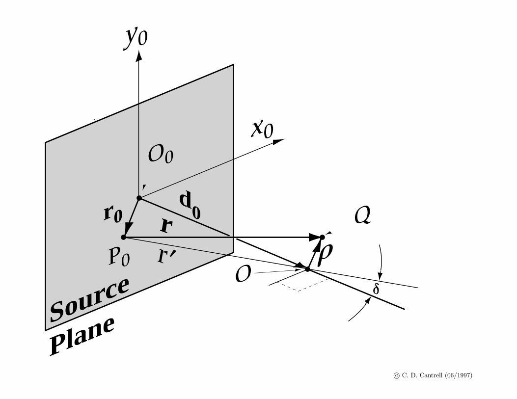
COORDINATES FOR THE flFRESNEL-KIRCHHOFF DIFFRACTION INTEGRAL
ρ
r1
r0
O0
d0
d1

The University of Texas at Dallas Erik Jonsson SchoolPhoTEC
c© C. D. Cantrell (06/1997)
FRESNEL-KIRCHHOFF DIFFRACTION THEORY (9)
• The Fresnel-Kirchhoff diffraction formula
u(x) = −ikA
4π
∫A
eik(r+s)
rs(n · s + n · r) dS
� is an approximate scalar solution of the Helmholtz equation, valid forwavelengths small compared to the aperture size
� is based on deep physical insight
� is accurate enough to give useful, quantitative results in opticsbut
� does not make u → 0 at large distances (as assumed in Kirchhoff’s bound-ary conditions)
� is not the first term in any iterative solution of the boundary-value prob-lem

The University of Texas at Dallas Erik Jonsson SchoolPhoTEC
c© C. D. Cantrell (06/1997)
FRESNEL-KIRCHHOFF DIFFRACTION THEORY (10)
• Consistency of the Fresnel-Kirchhoff diffraction formula
u(x) = −ikA
4π
∫A
eik(r+s)
rs(n · s + n · r) dS
with Huyghens’ Principle
� Expresses u(x) as a superposition of spherical waves eiks/s emanatingfrom the wavefront eikr/r produced by a point source
� The inclination factor is
I(r, s) = −(n · s + n · r)◦ In the backward direction (s = −r),
I(r,−r) = 0
◦ In the forward direction (s = r),
I(r, r) = −2 cos δ

The University of Texas at Dallas Erik Jonsson SchoolPhoTEC
c© C. D. Cantrell (06/1997)
FRESNEL-KIRCHHOFF DIFFRACTION THEORY (11)
• Extensions of the Fresnel-Kirchhoff diffraction formula:
� If the inclination factor is nearly constant over the aperture,
u(x) ≈ ikAI
4π
∫A
eik(r+s)
rsdS
� Replace the point-source incident wavefront eikr/r produced by a pointsource with a general wavefront uinc(r) produced by an extended source(modeled as a collection of point sources):
u(x) =ikI
4π
∫A
uinc(r)eiks
sdS
� Characterize the aperture by a transmission function τ to modelamplitude and/or phase changes due to lenses & diffraction gratings
u(x) =ikI
4π
∫A
τ (r) uinc(r)eiks
sdS

c© C. D. Cantrell (06/1997)
THIN LENS
ρ
d = cos θ
≈ 12 θ2
≈2
2
(1− )R
R
ρ
R
R
d
θ
Optical path in lens
t0
kn[t0− ]
2
2ρ
R
≈
ρ
The University of Texas at Dallas Erik Jonsson SchoolPhoTEC
c© C. D. Cantrell (06/1997)
TRANSMISSION FUNCTION OF A THIN LENS
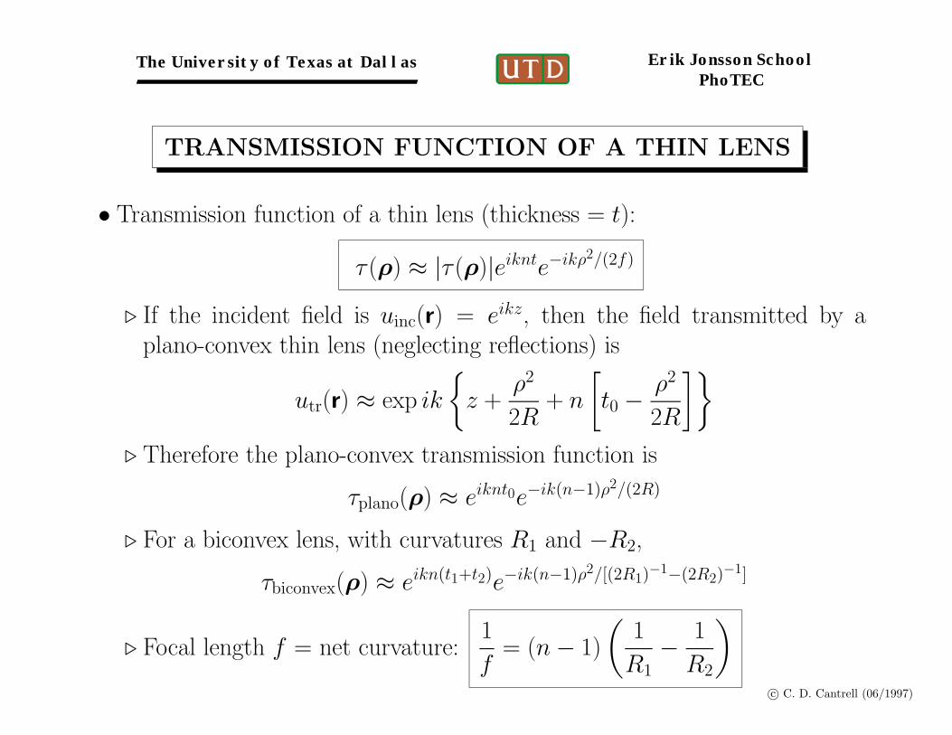
• Transmission function of a thin lens (thickness = t):
τ (ρ) ≈ |τ (ρ)|eiknte−ikρ2/(2f)
� If the incident field is uinc(r) = eikz, then the field transmitted by aplano-convex thin lens (neglecting reflections) is
utr(r) ≈ exp ik
{z +
ρ2
2R+ n
[t0 −
ρ2
2R
]}
� Therefore the plano-convex transmission function is
τplano(ρ) ≈ eiknt0e−ik(n−1)ρ2/(2R)
� For a biconvex lens, with curvatures R1 and −R2,
τbiconvex(ρ) ≈ eikn(t1+t2)e−ik(n−1)ρ2/[(2R1)−1−(2R2)
−1]
� Focal length f = net curvature:1
f= (n − 1)
(1
R1− 1
R2
)

The University of Texas at Dallas Erik Jonsson SchoolPhoTEC
c© C. D. Cantrell (06/1997)
DIFFRACTION THEORY (1)
• Applications of the Fresnel-Kirchhoff diffraction formula
u(x) =ikI
4π
∫A
τ (r) uinc(r)eiks
sdS
� Diffraction of light from a point source:
uinc(r) = Aeikr
r
◦ Fraunhofer limit (plane waves)
◦ Fresnel regime
� Diffraction theory of image formation
◦ Aberrations
◦ Focal-plane filtering
◦ Transfer functions
� Propagation of the mutual coherence function

The University of Texas at Dallas Erik Jonsson SchoolPhoTEC
c© C. D. Cantrell (06/1997)
DIFFRACTION THEORY (2)
• Fresnel’s approximation to a spherical wave:
eikr
r≈ eikr′
r′eik1·ρeik[ρ2−(r′·ρ)2]/(2r′)
�eikr′
r′= spherical wave centered at P0
� eik1·ρ = plane wave with propagation constant k1 := kr′
� eik[ρ2−(r′·ρ)2]/(2r′) = lowest correction for wavefront curvature
◦ This factor is approximately 1 when the Fresnel number is small:
b2
r′λ� 1
where b2 := ρ2 − (r′ · ρ)2
• Bottom line: You get a nearly plane wave if you move far away from a pointsource (but it’s easier to use a lens!)

c© C. D. Cantrell (06/1997)
THE FRESNEL APPROXIMATION
r
r
ρ
′
ρ
θ
a
b
a = r′ · ρb2 = ρ2 − a2 = ρ2 − (r′ · ρ)2
r =r′ + a
cos θ
≈ r′
cos θ+ a ≈ r′(1 + 1
2θ2) + a
≈ r′ + a +b2
2r′

The University of Texas at Dallas Erik Jonsson SchoolPhoTEC
c© C. D. Cantrell (06/1997)
FRESNEL APPROXIMATION DETAILS (1)
• Approximate r in terms of r′ (fixed) and ρ (varies over aperture):
� Vector addition:r = r′ + ρ
r2 = r′2+ 2r′ · ρ + ρ2
r = r′[1 + 2
r′
r′2· ρ +
(ρ
r′
)2]1/2
� Binomial expansion correct to order (ρ/r′)2:
r ≈ r′ +r′
r′· ρ +
ρ2
2r′− (r′ · ρ)2
2r′3
r ≈ r′ + r′ · ρ +ρ2
2r′− (r′ · ρ)2
2r′

The University of Texas at Dallas Erik Jonsson SchoolPhoTEC
c© C. D. Cantrell (06/1997)
FRESNEL APPROXIMATION DETAILS (2)
• The Fresnel approximation, valid for small angles between r and r′:
denominator = r ≈ r′
phase = kr ≈ kr′ + k1 · ρ + k
[ρ2 − (r′ · ρ)2
2r′
]
�eikr′
r′= spherical wave centered at P0
� eik1·ρ = plane wave with direction r′
◦ Propagation constant: k1 := kr′
� eik[ρ2−(r′·ρ)2]/(2r′) = lowest-order approximation to the phase of a sphericalwavefront
eikr
r≈ eikr′
r′eik1·ρeik[ρ2−(r′·ρ)2]/(2r′)
y0
x0
OP0
Q
δ
′rr
Source
Plane
ρ
r0
O0
d0
c© C. D. Cantrell (06/1997)

y0
x0
η
ξ y1
x1
Observation
Plane
Screen
OP0
P
Q
′sδ
′r sr
Source
Plane
c© C. D. Cantrell (06/1997)
COORDINATES FOR THE flFRESNEL-KIRCHHOFF DIFFRACTION INTEGRAL
ρ
r1
r0
O0
d0
d1

c© C. D. Cantrell (06/1997)
COORDINATES FOR THE DIFFRACTION INTEGRAL
r
s
r
ρ
′s ′
r1
k1
–k2
q

The University of Texas at Dallas Erik Jonsson SchoolPhoTEC
c© C. D. Cantrell (06/1997)
DIFFRACTION THEORY (3)
• Diffraction pattern of a point source, part 1:
� Fresnel’s approximation applied to the spherical waves eikr/r and eiks/s:
eikr
r≈ eikr′
r′eik1·ρ exp
{ik
[ρ2 − (r′ · ρ)2
2r′
]}
eiks
s≈ eiks′
s′eik2·(r1−ρ) exp
{ik
[(r1 − ρ)2 − [s′ · (r1 − ρ)]2
2s′
]}
where the propagation vectors are
k1 := kr′, k2 := ks′, q := k1 − k2
� Diffraction integral for a point source in Fresnel’s approximation:
u(x) =ikIAeik(r′+s′)
4πr′s′eik2·r1
∫A
τ (r) eiq·ρeik
[ρ2−(r′·ρ)2
2r′ +(r1−ρ)2−[s′·(r1−ρ)]2
2s′
]dS

The University of Texas at Dallas Erik Jonsson SchoolPhoTEC
c© C. D. Cantrell (06/1997)
DIFFRACTION THEORY (4)
• Diffraction pattern of a point source, part 2:
� Diffraction integral for a point source in Fresnel’s approximation:
u(x) =ikIAeik(r′+s′)
4πr′s′eik2·r1
∫A
τ (ρ) eiq·ρeik
[ρ2−(r′·ρ)2
2r′ +(r1−ρ)2−[s′·(r1−ρ)]2
2s′
]dS
where q := k1 − k2, k1 := kr′, k2 := ks′
� eik2·r1 = plane wave “carrier” incident at P
� Integral over aperture = “signal”
◦ eik
[ρ2−(r′·ρ)2
2r′ +(r1−ρ)2−[s′·(r1−ρ)]2
2s′
]= wavefront curvature correction
◦ Fresnel diffraction: Wavefront curvature is an essential part of thephysics
◦ Fraunhofer diffraction: No wavefront curvature correction needed
u(x) =
∫A
τ (ρ) eiq·ρ dS
= Fourier transform of τ

The University of Texas at Dallas Erik Jonsson SchoolPhoTEC
c© C. D. Cantrell (06/1997)
DIFFRACTION THEORY (5)
• Fraunhofer diffraction at a rectangular aperture:
u(x) =
∫A
τ (ρ) eiq·ρ dS
where q := k1 − k2, k1 := kr′, k2 := ks′
� Aperture dimensions: 2a (in x) × 2b (in y)
� q is not necessarily in the plane of the aperture, but we can assume thatit is for this case because its z-component is small
� Integral over the components of ρ:
u(r1) =ikIAeik(r′+s′)
4πr′s′eik2·r1
∫ a
−a
∫ b
−b
ei(qxξ+qyη)
= (constant)[2 sinc (qxa)][2 sinc (qyb)]
dξ dη
� Intensity:
S(q) = S(0) sinc2(qxa) sinc2(qyb)


The University of Texas at Dallas Erik Jonsson SchoolPhoTEC
c© C. D. Cantrell (06/1997)
DIFFRACTION THEORY (6)
• Fraunhofer diffraction at a circular aperture:
u(x) =
∫A
τ (ρ) eiq·ρ dS
where q := k1 − k2, k1 := kr′, k2 := ks′
� Aperture radius = a
� Integral over the components of ρ:
u(q) =ikIAeik(r′+s′)
4πr′s′eik2·r1
∫ 2π
0
∫ a
0
eiqρ cos φ ρ dρ dφ
= (constant)(πa2)
[2J1(qa)
qa
]
� Intensity:
S(q) = S(0)
[2J1(qa)
qa
]2
(the Airy pattern)


The University of Texas at Dallas Erik Jonsson SchoolPhoTEC
c© C. D. Cantrell (06/1997)
DIFFRACTION THEORY (7)
• Dimensions of central feature:
� Rectangular aperture, 2a × 2b
◦ For a small diffraction angle, qx ≈ kξ
s′, qy ≈ k
η
s′◦ First zero of sinc function is at x = π
◦ At the first zero in ξ,2π
λ
ξ0
s′a = π
ξ0 =λs′
2a, η0 =
λs′
2b
� Circular aperture, radius a
◦ For a small diffraction angle θ, q ≈ kθ
◦ First zero of J1 is j1,1 = 3.832 · · · = 1.220π
◦ At the first zero, qa ≈ 2πθ0a/λ ≈ 1.220π
θ0 ≈ 0.610λ
a≈ 1.220
λ
d

The University of Texas at Dallas Erik Jonsson SchoolPhoTEC
c© C. D. Cantrell (06/1997)
DIFFRACTION THEORY (8)
• Fraunhofer diffraction by N randomly arranged identical apertures:
� Aperture Am is displaced from aperture A1 by a random vector am
� Amplitude of diffracted field is proportional to∫A
eiq·ρ dS =
N∑m=1
eiq·am
∫A1
eiq·ρ dS
� Intensity of diffracted field is
S(q) = (const.)
∣∣∣∣∣N∑
m=1
eiq·am
∫A1
eiq·ρ dS
∣∣∣∣∣2
= (const.)
N∑m=1
N∑n=1
eiq·(am−an)
∣∣∣∣∫
A1
eiq·ρ dS
∣∣∣∣2
= N × (const.) ×∣∣∣∣∫
A1
eiq·ρ dS
∣∣∣∣2
∣∣∣∣∫
A1
eiq·ρ dS
∣∣∣∣2
∝ diffraction pattern of a single aperture
� Intensities add, not amplitudes, when the arrangement is random
The University of Texas at Dallas Erik Jonsson SchoolPhoTEC
c© C. D. Cantrell (06/1997)
DIFFRACTION THEORY (9)
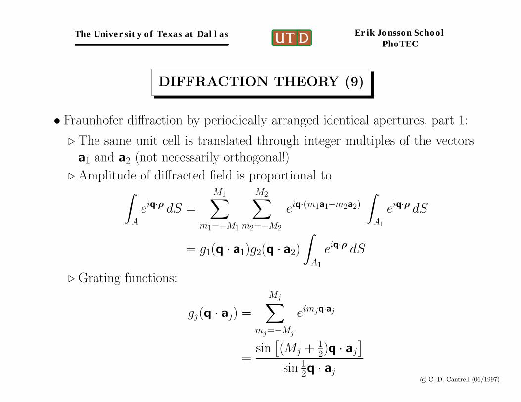
• Fraunhofer diffraction by periodically arranged identical apertures, part 1:
� The same unit cell is translated through integer multiples of the vectorsa1 and a2 (not necessarily orthogonal!)
� Amplitude of diffracted field is proportional to∫A
eiq·ρ dS =
M1∑m1=−M1
M2∑m2=−M2
eiq·(m1a1+m2a2)
∫A1
eiq·ρ dS
= g1(q · a1)g2(q · a2)
∫A1
eiq·ρ dS
� Grating functions:
gj(q · aj) =
Mj∑mj=−Mj
eimjq·aj
=sin
[(Mj + 1
2)q · aj
]sin 1
2q · aj

0 2 4 6
-20
0
20
40
60
g(x) =sin
[(M+ 1
2)x]
sin( x)12
x
g(x)
THE GRATING FUNCTION
c© C. D. Cantrell (06/1997)
for M = 20

The University of Texas at Dallas Erik Jonsson SchoolPhoTEC
c© C. D. Cantrell (06/1997)
DIFFRACTION THEORY (10)
• Fraunhofer diffraction by periodically arranged identical apertures, part 2:
� Properties of the grating function
g(q · a) =sin
[(M + 1
2)q · a]
sin 12q · a
◦ Peak value of g is 2M + 1 at
q · a = 2nπ
◦ Half-width of central peak =π
M + 12
◦ Amplitude of first side lobe is −0.212× amplitude of central peak

The University of Texas at Dallas Erik Jonsson SchoolPhoTEC
c© C. D. Cantrell (06/1997)
DIFFRACTION THEORY (11)
• Fraunhofer diffraction by periodically arranged identical apertures, part 3:
� Intensity of diffracted field is proportional to∣∣∣∣∫
A
eiq·ρ dS
∣∣∣∣2
= |g1(q · a1)|2 |g2(q · a2)|2∣∣∣∣∫
A1
eiq·ρ dS
∣∣∣∣2
◦ The grating functions are sharply peaked at values of q such that
q · a1 = 2n1π and q · a2 = 2n2π
� These conditions imply that q is 2π times a reciprocal lattice vector:
q = 2π(n1b1 + n2b2)
◦ Peaks are modulated by the diffraction pattern of a single aperture,∣∣∣∣∫
A1
eiq·ρ dS
∣∣∣∣2

The University of Texas at Dallas Erik Jonsson SchoolPhoTEC
c© C. D. Cantrell (06/1997)
2-D RECIPROCAL LATTICE (1)
• The 2-d direct lattice spanned by non-parallel vectors a1 and a2
consists of the pointsrm1,m2 = m1a1 + m2a2
• The reciprocal lattice to the a1 – a2 lattice consists of vectors
kn1,n2 = n1b1 + n2b2
wherebi · aj = δi,j
� The reciprocal lattice basis is
b1 =a2 × z
z · (a1 × a2), b2 =
z × a1
z · (a1 × a2)
Hexagonal lattice basis: a1 = x, a2 =1
2x +
√3
2y
Reciprocal lattice basis: b1 = x − 1√3y, b2 =
2√3y
The University of Texas at Dallas Erik Jonsson SchoolPhoTEC
c© C. D. Cantrell (06/1997)
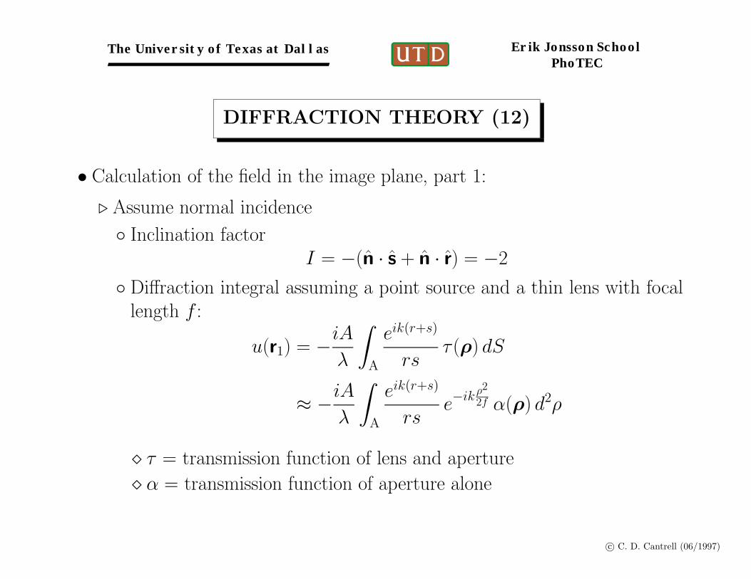
DIFFRACTION THEORY (12)
• Calculation of the field in the image plane, part 1:
� Assume normal incidence
◦ Inclination factorI = −(n · s + n · r) = −2
◦ Diffraction integral assuming a point source and a thin lens with focallength f :
u(r1) = −iA
λ
∫A
eik(r+s)
rsτ (ρ) dS
≈ −iA
λ
∫A
eik(r+s)
rse−ik ρ2
2f α(ρ) d2ρ
� τ = transmission function of lens and aperture
� α = transmission function of aperture alone

The University of Texas at Dallas Erik Jonsson SchoolPhoTEC
c© C. D. Cantrell (06/1997)
DIFFRACTION THEORY (13)
• Calculation of the field in the image plane, part 2:
� Diffraction integral assuming a point source and a thin lens with focallength f :
u(r1) ≈ −iA
λ
∫A
eik(r+s)
rse−ik ρ2
2f α(ρ) d2ρ
◦ The sum of the exponents is (in the Fresnel approximation)
ik
[r + s − ρ2
2f
]≈ ik
[r′ + s′ − ρ2
2f+
(r0 − ρ)2
2r′+
(ρ − r1)2
2s′
]
= ik
[r′ + s′ +
ρ2
2
(−1
f+
1
r′+
1
s′
)+
r20
2r′+
r21
2s′− ρ ·
(r0r′
+r1s′
)]

The University of Texas at Dallas Erik Jonsson SchoolPhoTEC
c© C. D. Cantrell (06/1997)
DIFFRACTION THEORY (14)
• Calculation of the field in the image plane, part 3:
� At the Gaussian focal point of a thin lens,
−1
f+
1
r′+
1
s′= 0
◦ This makes the coefficient of ρ2 vanish in the exponent
◦ The diffraction integral reduces to a phase factor times the Fouriertransform of the pupil function α:
u(r1) ≈ − iA
λr′s′eik
[(r202r′+
r212s′
)+r′+s′
] ∫A
α(ρ) e−ikρ·(r0r′+
r1s′ ) d2ρ
◦ The image is spread out by diffraction
◦ The peak amplitude occurs at the stationary-phase point:
r0r′
+r1s′
= 0 ⇒ r1 = −s′
r′r0 (Gaussian image displacement)

The University of Texas at Dallas Erik Jonsson SchoolPhoTEC
c© C. D. Cantrell (06/1997)
DIFFRACTION THEORY (15)
• Imaging by a thin lens of an extended, coherently illuminated object:
� Superpose the fields due to a distribution ψ of point sources:
u(r1) ≈ − i
λ
∫S
∫A
ψ(r0)eikr
rα(ρ) e−ik ρ2
2feiks
sd2ρ d2r0
◦ Instead of performing two 2-d integrations simultaneously, we can eval-uate a diffraction integral to go from the source to the lens and anotherto go from the lens to the observation plane
◦ Field incident at lens:
uinc(ρ) ≈ − i
λ
eikr′
r′
∫S
ψ(r0) eik(ρ−r0)2
2r′ d2r0
≈ − i
λ
eikr′
r′
∫S
ψ(r0) Fk/r′(ρ − r0) d2r0
� uinc is a convolution of the source distribution ψ with the Fresnelfunction Fk/r′, where
Fα(r) := eiαr2

The University of Texas at Dallas Erik Jonsson SchoolPhoTEC
c© C. D. Cantrell (06/1997)
THE FRESNEL FUNCTION (1)
• The Fresnel function is
Fα(r) := e12iαr2
where r lies in the x – y plane
� The 2-d Fourier transform of Fα is
Fα(q) =
∫e−iq·r Fα(r) d2r
=2iπ
αF−1/α(q)
=2iπ
αe−i q2
2α

The University of Texas at Dallas Erik Jonsson SchoolPhoTEC
c© C. D. Cantrell (06/1997)
DIFFRACTION THEORY (16)
• Imaging by a thin lens of an extended, coherently illuminated object, part2:
� The field incident on the lens, uinc, is a convolution of the source distri-bution ψ with the Fresnel function Fk/r′:
uinc(ρ) = − i
λ
eikr′
r′
∫S
ψ(r0) Fk/r′(ρ − r0) d2r0
= − i
λ
eikr′
r′1
(2π)2
∫ψ(q) Fk/r′(q) eiq·ρ d2q
� Diffraction integral for the field in the observation plane:
u(r1) =
(− i
λ
)2eik(r′+s′)
(2π)2r′s′
∫ ∫A
ψ(q) Fk/r′(q) α(ρ) eE(q,ρ,r1) d2ρ d2q
◦ The sum of the exponents is (in the Fresnel approximation)
E(q, ρ, r1) = ik
[−ρ2
2f+
ρ2
2s′+
r21
2s′
]+ i
(q − k
r1s′
)· ρ

The University of Texas at Dallas Erik Jonsson SchoolPhoTEC
c© C. D. Cantrell (06/1997)
DIFFRACTION THEORY (17)
• Imaging by a thin lens of an extended, coherently illuminated object, part3:
� In the back focal planes′ = f
the sum of the exponents does not depend on ρ2:
E(q, ρ, r1) = ikr21
2s′+ iq′ · ρ
where
r′1 := r1|s′=f and q′ := q − kr′1s′
� Diffraction integral for the field in the back focal plane:
u(r′1) =
(− i
λ
)2eik(r′+s′)
(2π)2r′s′eik
r′12
2f
∫ψ(q) Fk/r′(q) α(q′) d2q

The University of Texas at Dallas Erik Jonsson SchoolPhoTEC
c© C. D. Cantrell (06/1997)
DIFFRACTION THEORY (18)
• Imaging by a thin lens of an extended, coherently illuminated object, part4:
� Diffraction integral for the field in the back focal plane:
u(r′1) =
(− i
λ
)2eik(r′+s′)
(2π)2r′s′eik
r′12
2f
∫ψ(q) Fk/r′(q) α(q′) d2q
� The Fourier transform of the pupil function, α, is very sharply peaked atq′ = 0 (for a circular pupil, α is the Airy disk)
◦ For an infinite aperture, α(q′) = (2π)2δ(q′) ⇒ q = kr′1f
◦ In this limit, and with the Fraunhofer approximation,
u(r′1) ≈ − i
λfψ
(kr′1f
)
◦ The back focal plane contains the Fourier transform of acoherently illuminated object

The University of Texas at Dallas Erik Jonsson SchoolPhoTEC
c© C. D. Cantrell (06/1997)
DIFFRACTION THEORY (19)
• Imaging by a thin lens of an extended, coherently illuminated object, part5: Focal plane filtering
� Concept: Alter the image by (intentionally or unintentionally)filtering the Fourier transform in the focal plane
� Propagate the field from the back focal plane to the image plane usingyet another diffraction integral!
� Field in the image plane:
u(r1) = − i
λ
∫F
eiku
uσ(r′1) u(r′1) d2r′1
◦ Focal-plane filter transmission function = σ
◦ Vector from point in focal plane to point in image plane:
u = s′′ + r1 − r′1

The University of Texas at Dallas Erik Jonsson SchoolPhoTEC
c© C. D. Cantrell (06/1997)
DIFFRACTION THEORY (20)
• Imaging by a thin lens of an extended, coherently illuminated object, part 6
� Propagate the field from the back focal plane to the image plane
◦ Assume an infinite aperture, α(q′) = (2π)2δ(q′):
u(r′1) ≈ − i
λfe
ikr′12
2
(1f−
r′f2
)ψ
(kr′1s′
)
◦ Sum of exponents in the diffraction integral:
ikr′12
2
(1
f− r′
f 2+
1
s′′
)
◦ Use Newton’s equation for the focus-to-image distance rI :
1
f− r′
f 2=
f − r′
f 2=
1
f − rI
◦ All quadratic phase terms cancel in the image plane, f − rI = −s′′

The University of Texas at Dallas Erik Jonsson SchoolPhoTEC
c© C. D. Cantrell (06/1997)
DIFFRACTION THEORY (21)
• Imaging by a thin lens of an extended, coherently illuminated object, part 7
� Field amplitude in the image plane:
u(r′1) ≈ −(
i
λ
)21
(2π)2s′′fei
kr212s′′
∫F
σ(r′1) ψ
(kr′1f
)e−ik
r′1·r1s′′ d2r′1
◦ The image-plane field is proportional to the Fouriertransform of the product of the focal-plane filteringfunction σ and the Fourier transform of the original field