Integer Programminguetzm/do/IP-FKS.pdf · CHAPTER 9 Integer Programming An integer linear program...
24
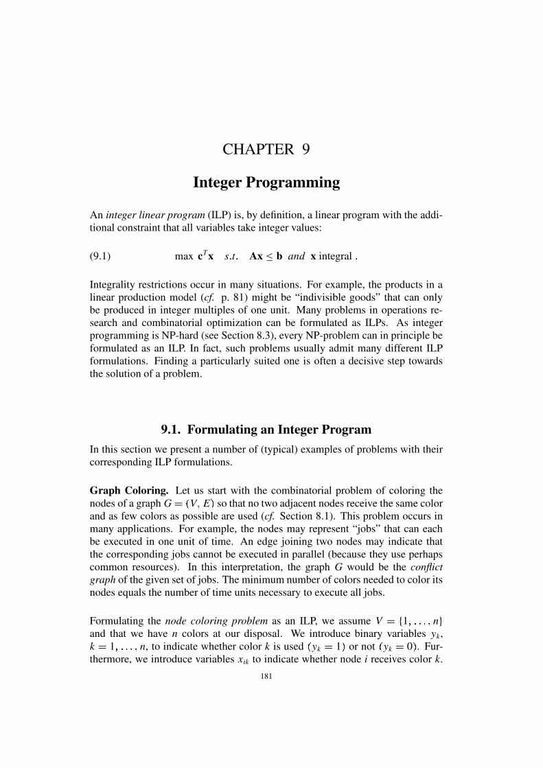
CHAPTER 9 Integer Programming An integer linear program (ILP) is, by definition, a linear program with the addi- tional constraint that all variables take integer values: (9.1) max c T x st Ax ≤ b and x integral Integrality restrictions occur in many situations. For example, the products in a linear production model (cf. p. 81) might be “indivisible goods” that can only be produced in integer multiples of one unit. Many problems in operations re- search and combinatorial optimization can be formulated as ILPs. As integer programming is NP-hard (see Section 8.3), every NP-problem can in principle be formulated as an ILP. In fact, such problems usually admit many different ILP formulations. Finding a particularly suited one is often a decisive step towards the solution of a problem. 9.1. Formulating an Integer Program In this section we present a number of (typical) examples of problems with their corresponding ILP formulations. Graph Coloring. Let us start with the combinatorial problem of coloring the nodes of a graph G = VE so that no two adjacent nodes receive the same color and as few colors as possible are used (cf. Section 8.1). This problem occurs in many applications. For example, the nodes may represent “jobs” that can each be executed in one unit of time. An edge joining two nodes may indicate that the corresponding jobs cannot be executed in parallel (because they use perhaps common resources). In this interpretation, the graph G would be the conflict graph of the given set of jobs. The minimum number of colors needed to color its nodes equals the number of time units necessary to execute all jobs. Formulating the node coloring problem as an ILP, we assume V ={1 n} and that we have n colors at our disposal. We introduce binary variables y k , k = 1 n, to indicate whether color k is used y k = 1 or not y k = 0 . Fur- thermore, we introduce variables x ik to indicate whether node i receives color k. 181
Transcript of Integer Programminguetzm/do/IP-FKS.pdf · CHAPTER 9 Integer Programming An integer linear program...
CHAPTER 9
Integer Programming
An integer linear program (ILP) is, by definition, a linear program with the addi-tional constraint that all variables take integer values:
(9.1) max cTx s � t � Ax ≤ b and x integral �Integrality restrictions occur in many situations. For example, the products in alinear production model (cf. p. 81) might be “indivisible goods” that can onlybe produced in integer multiples of one unit. Many problems in operations re-search and combinatorial optimization can be formulated as ILPs. As integerprogramming is NP-hard (see Section 8.3), every NP-problem can in principle beformulated as an ILP. In fact, such problems usually admit many different ILPformulations. Finding a particularly suited one is often a decisive step towardsthe solution of a problem.
9.1. Formulating an Integer ProgramIn this section we present a number of (typical) examples of problems with theircorresponding ILP formulations.
Graph Coloring. Let us start with the combinatorial problem of coloring thenodes of a graph G= � V � E � so that no two adjacent nodes receive the same colorand as few colors as possible are used (cf. Section 8.1). This problem occurs inmany applications. For example, the nodes may represent “jobs” that can eachbe executed in one unit of time. An edge joining two nodes may indicate thatthe corresponding jobs cannot be executed in parallel (because they use perhapscommon resources). In this interpretation, the graph G would be the conflictgraph of the given set of jobs. The minimum number of colors needed to color itsnodes equals the number of time units necessary to execute all jobs.
Formulating the node coloring problem as an ILP, we assume V = {1 � ����� � n}and that we have n colors at our disposal. We introduce binary variables yk,k = 1 � ����� � n, to indicate whether color k is used � yk = 1 � or not � yk = 0 � . Fur-thermore, we introduce variables xik to indicate whether node i receives color k.
181
182 9. INTEGER PROGRAMMING
The resulting ILP is
(9.2) min∑n
k=1 yk s � t � � 1 � ∑nk=1 xik = 1 i = 1 � ����� � n� 2 � xik − yk ≤ 0 i � k = 1 � ����� � n� 3 � xik + x jk ≤ 1 � i � j � ∈ E � k = 1 � ����� � n� 4 � 0 ≤ xik � yk ≤ 1� 5 � xik � yk ∈ Z
The constraints (4) and (5) ensure that the xik and yk are binary variables. Theconstraints (1)–(3) guarantee (in this order) that each node is colored, node i re-ceives color k only if color k is used at all, and any two adjacent nodes havedifferent colors.
EX. 9.1. Show: If the integrality constraint (5) is removed, the resulting linear programhas optimum value equal to 1.
The Traveling Salesman Problem (TSP). This is one of the best-known com-binatorial optimization problems: There are n towns and a ”salesman”, locatedin town 1, who is to visit each of the other n − 1 towns exactly once and thenreturn home. The tour (traveling salesman tour) has to be chosen so that the to-tal distance traveled is minimized. To model this problem, consider the so-calledcomplete graph Kn, i.e., the graph Kn = � V � E � with n = |V | pairwise adjacentnodes. With respect to a given cost (distance) function c : E→ R we then seekto find a Hamilton circuit C ⊆ E, i.e., a circuit including every node, of minimalcost.
An ILP formulation can be obtained as follows. We introduce binary variablesxik � i � k = 1 � ����� � n � to indicate whether node i is the kth node visited. In addition,we introduce variables ye � e ∈ E � to record whether edge e is traversed:
(9.3)
min∑
e∈E ce ye
s � t � x11 = 1∑nk=1 xik = 1 i = 1 � ����� � n∑ni=1 xik = 1 k = 1 � ����� � n∑
e ye = nxi + k−1+ x jk − ye ≤ 1 e = � i � j � � k ≥ 2
xin + x11 − ye ≤ 1 e = � i � 1 �0 ≤ xik � ye ≤ 1
xik � ye ∈ Z
EX. 9.2. Show that each feasible solution of (9.3) corresponds to a Hamilton circuit andconversely.
In computational practice, other TSP formulations have proved more efficient.To derive an alternative formulation, consider first the following simple programwith edge variables ye, e ∈ E:
9.1. FORMULATING AN INTEGER PROGRAM 183
(9.4)min cTy s � t � y �J�t� i ��� = 2 i = 1 � ����� � n
0 ≤ y ≤ 1y integral �
(Recall our shorthand notation y �-�7� i ��� =∑e∈ " � i � ye for the sum of all y-values onedges incident with node i.)
ILP (9.4) does not describe our problem correctly: We still must rule out solu-tions corresponding to disjoint circuits that cover all nodes. We achieve this byadding more inequalities, so-called subtour elimination constraints. To simplifythe notation, we write for y ∈ RE and two disjoint subsets S � T ⊆ V
y � S : T � = ∑
e = e i ¡ j fi ∈ S ¡ j ∈ T
ye �
The subtour elimination constraints
y � S : S � ≥ 2
make sure that there will be at least two edges in the solution that lead from aproper nonempty subset S⊂ V to its complement S= V \ S. So the correspondingtour is connected. A correct ILP-formulation is thus given by
(9.5)
min cTy s � t � y �J�t� i ��� = 2 i = 1 � ����� � ny � S : S � ≥ 2 ∅ ⊂ S ⊂ V0 ≤ y ≤ 1
y integral �Note the contrast to our first formulation (9.3): ILP (9.5) has exponentially manyconstraints, one for each proper subset S ⊂ V . If n = 30, there are more than 230
constraints. Yet, the way to solve (9.5) in practice is to add even more constraints!This approach of adding so-called cutting planes is presented in Sections 9.2 and9.3 below.
REMARK. The mere fact that (9.5) has exponentially many constraints does not preventus from solving it (without the integrality constraints) efficiently (cf. Section 10.6.2).
Maximum Clique. This is another well-studied combinatorial problem, whichwe will use as a case study for integer programming techniques later. Consideragain the complete graph Kn = � V � E � on n nodes. This time, there are weightsc ∈ RV and d ∈ RE given on both the vertices and the edges. We look for a setC ⊆ V that maximizes the total weight of vertices and induced edges:
(9.6) maxC⊆V
c � C � + d � E � C ��� �As Kn = � V � E � is the complete graph, each C ⊆ V is a clique (set of pairwiseadjacent nodes). Therefore, we call (9.6) the maximum weighted clique problem.
184 9. INTEGER PROGRAMMING
EX. 9.3. Given a graph G = � V E ′ � with E′ ⊆ E, choose c = 1 and
de ={
0 e ∈ E′
−n otherwise
Show: With these parameters (for Kn = � V E � ), (9.6) reduces to the problem of findinga clique C in G of maximum cardinality.
Problem (9.6) admits a rather straightforward ILP-formulation:
(9.7)
max cTx+ dTyye − xi ≤ 0 e ∈ E � i ∈ e
xi + x j − ye ≤ 1 e = � i � j � ∈ E0 ≤ x � y ≤ 1
x � y integer
A vector � x � y � with all components xi � ye ∈ {0 � 1} that satisfies the constraints of(9.7) is the so-called (vertex-edge) incidence vector of the clique
C = {i ∈ V | xi = 1} �In other words, x ∈ RV is the incidence vector of C and y ∈ RE is the incidencevector of E � C � .REMARK. The reader may have noticed that all ILPs we have formulated so far arebinary programs, i.e., the variables are restricted to take values in {0 1} only. This isnot by pure accident. The majority of integer optimization problems can be cast in thissetting. But of course, there are also others (e.g., the integer linear production modelmentioned in the introduction to this chapter).
9.2. Cutting Planes IConsider the integer linear program
(9.8) max cTx s � t � Ax ≤ b and x integral �For the following structural analysis it is important (see Ex. 9.4) to assume that Aand b are rational, i.e., A ∈ Qm×n and b ∈ Qm. In this case, the polyhedron
(9.9) P = {x ∈ Rn | Ax ≤ b}is a rational polyhedron (cf. Section 3.6). The set of integer vectors in P is adiscrete set, whose convex hull we denote by
(9.10) PI = conv {x ∈ Zn | Ax ≤ b} �Solving (9.8) is equivalent with maximizing cTx over the convex set PI (Why?).Below, we shall prove that also PI is a polyhedron and derive a system of inequal-ities describing PI. We thus show how (at least in principle) the original problem(9.8) can be reduced to a linear program.
EX. 9.4. Give an example of a (non-rational) polyhedron P ⊆ Rn such that the set PI isnot a polyhedron.
9.2. CUTTING PLANES I 185
PROPOSITION 9.1. Let P ⊆ Rn be a rational polyhedron. Then also PI is arational polyhedron. In case PI 6= ∅, its recession cone equals that of P.
Proof. The claim is trivial if P is bounded (as P then contains only finitely manyinteger points and the result follows by virtue of the discussion in Section 3.6). Bythe Weyl-Minkowski Theorem 3.2, a rational polyhedron generally decomposesinto
P = conv V + cone Wwith finite sets of rational vectors V ⊆ Qn and W ⊆ Qn. By scaling, if necessary,we may assume that W ⊆ Zn. Denote by V and W the matrices whose columnsare the vectors in V and W respectively. Thus each x ∈ P can be written as
x = Vλ+Wµ � where λ � µ ≥ 0 and 1Tλ = 1 �Let bµc be the integral part of µ 6= 0 (obtained by rounding down each compo-nent O i ≥ 0 to the next integer b O ic). Splitting µ into its integral part bµc and itsnon-integral part µ = µ− bµc yields
x = Vλ+Wµ+Wbµc = x+Wbµcwith bµc ≥ 0 integral and x ∈ P, where
P = {Vλ+Wµ | λ ≥ 0 � 1Tλ = 1 � 0 ≤ µ � 1} �Because W ⊆ Zn, x is integral if and only if x is integral. Hence
P∩Zn = P∩Zn + {Wz | z ≥ 0 integral} �Taking convex hulls on both sides, we find (cf. Ex. 9.5)
PI = conv � P∩Zn � + cone W �Since P is bounded, P∩Zn is finite. So the claim follows as before.
�
EX. 9.5. Show: conv � V +W � = conv V + conv W for all V W ⊆ Rn.
We next want to derive a system of inequalities describing PI . There is no loss ofgenerality when we assume P to be described by a system Ax ≤ b with A and bintegral. The idea now is to derive new inequalities that are valid for PI (but notnecessarily for P) and to add these to the system Ax ≤ b. Such inequalities arecalled cutting planes as they “cut off” parts of P that are guaranteed to contain nointegral points.
Consider an inequality cTx ≤ V that is valid for P. If c ∈ Zn but V 6∈ Z, theneach integral x ∈ P ∩ Zn obviously satisfies the stronger inequality cTx ≤ b V c.Recall from Corollary 2.6 that valid inequalities for P can be derived from thesystem Ax≤ b by taking nonnegative linear combinations. We therefore considerinequalities of the form
(9.11) � yTA � x ≤ yTb � y ≥ 0 �
186 9. INTEGER PROGRAMMING
If yTA ∈ Zn, then every x ∈ P∩Zn (and hence every x ∈ PI) satisfies
(9.12) � yTA � x ≤ byTbc �We say that (9.12) arises from (9.11) by rounding (if yTA ∈ Zn). In particular, weregain the original inequalities Ax ≤ b taking as y all unit vectors. We conclude
PI ⊆ P′ = {x ∈ Rn | � yTA � x ≤ byTbc � y ≥ 0 � yTA ∈ Zn} ⊆ P �Searching for inequalities of type (9.12) with yTA ∈ Zn, we may restrict ourselvesto 0 ≤ y ≤ 1. Indeed, each y ≥ 0 splits into its integral part z = byc ≥ 0 andnon-integral part y = y − z. The inequality (9.12) is then implied by the twoinequalities
(9.13)� zTA � x ≤ zTb � ∈ Z �� yTA � x ≤ byTbc �
(Recall that we assume A and b to be integral.) The first inequality in (9.13) isimplied by Ax≤ b. To describe P′, it thus suffices to augment the system Ax ≤ bby all inequalities of the type (9.12) with 0 ≤ y � 1, which describes
(9.14) P′ = {x ∈ Rn | � yTA � x ≤ byTbc � 0 ≤ y ≤ 1 � yTA ∈ Zn} �by a finite number of inequalities (see Ex. 9.6) and thus exhibits P′ as a polyhe-dron.
EX. 9.6. Show: There are only finitely many vectors yTA ∈ Zn with 0 ≤ y ≤ 1.
EX. 9.7. Show: P ⊆ Q implies P′ ⊆ Q′. (In particular, P′ depends only on P and noton the particular system Ax ≤ b describing P.)
Iterating the above construction, we obtain the so-called Gomory sequence
(9.15) P ⊇ P′ ⊇ P′′ ⊇ ����� ⊇ P � k � ⊇ ����� ⊇ PI �Remarkably (cf. Gomory [34], and also Chvatal [9]), Gomory sequences are al-ways finite:
THEOREM 9.1. The Gomory sequence is finite in the sense that P � t � = PI holdsfor some t ∈ N.
Before giving the proof, let us examine in geometric terms what it means to passfrom P to P′. Consider an inequality
� yTA � x ≤ yTb
with y ≥ 0 and yTA ∈ Zn. Assume that the components of yTA have greatestcommon divisor d = 1 (otherwise replace y by d−1y). Then the equation
� yTA � x = byTbc
9.2. CUTTING PLANES I 187
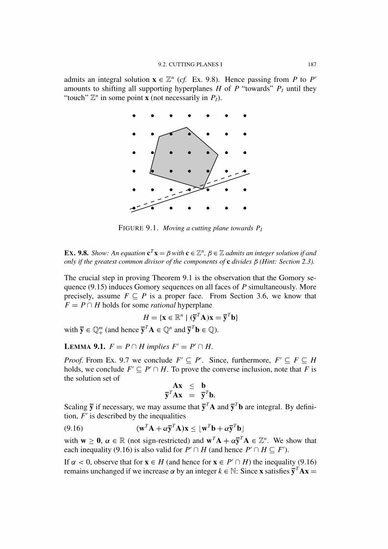
admits an integral solution x ∈ Zn (cf. Ex. 9.8). Hence passing from P to P′
amounts to shifting all supporting hyperplanes H of P “towards” PI until they“touch” Zn in some point x (not necessarily in PI).
FIGURE 9.1. Moving a cutting plane towards PI
EX. 9.8. Show: An equation cT x= ' with c ∈ Zn, ' ∈ Z admits an integer solution if andonly if the greatest common divisor of the components of c divides ' (Hint: Section 2.3).
The crucial step in proving Theorem 9.1 is the observation that the Gomory se-quence (9.15) induces Gomory sequences on all faces of P simultaneously. Moreprecisely, assume F ⊆ P is a proper face. From Section 3.6, we know thatF = P∩ H holds for some rational hyperplane
H = {x ∈ Rn | � yTA � x = yTb}with y ∈ Qm
+ (and hence yTA ∈ Qn and yTb ∈ Q).
LEMMA 9.1. F = P∩ H implies F ′ = P′ ∩ H.
Proof. From Ex. 9.7 we conclude F ′ ⊆ P′. Since, furthermore, F ′ ⊆ F ⊆ Hholds, we conclude F ′ ⊆ P′ ∩ H. To prove the converse inclusion, note that F isthe solution set of
Ax ≤ byTAx = yTb �
Scaling y if necessary, we may assume that yTA and yTb are integral. By defini-tion, F′ is described by the inequalities
(9.16) � wTA+ 1 yTA � x ≤ bwTb+ 1 yTbcwith w ≥ 0, 1 ∈ R (not sign-restricted) and wTA+ 1 yTA ∈ Zn. We show thateach inequality (9.16) is also valid for P′ ∩ H (and hence P′ ∩ H ⊆ F′).
If 1¢� 0, observe that for x ∈ H (and hence for x ∈ P′ ∩ H) the inequality (9.16)remains unchanged if we increase 1 by an integer k ∈ N: Since x satisfies yTAx=
188 9. INTEGER PROGRAMMING
yTb ∈ Z, both the left and right hand side will increase by kyTb if 1 is increased to1 + k. Hence we can assume 1 ≥ 0 without loss of generality. If 1 ≥ 0, however,(9.16) is easily recognized as an inequality of type (9.12). (Take y=w+ 1 y≥ 0.)So the inequality is valid for P′ and hence for P′ ∩ H.
�We are now prepared for the
Proof of Theorem 9.1. In case P = {x ∈ Rn | Ax = b} is an affine subspace, theclaim follows from Corollary 2.2 (cf. Ex. 9.9). In general, P is presented in theform
(9.17) Ax = bA′x ≤ b′
with n − d equalities Ai·x = bi and s ≥ 0 facet inducing (i.e., irredundant) in-equalities A′j·x ≤ b′j.
CASE 1: PI = ∅. Let us argue by induction on s ≥ 0. If s = 0, P is an affinesubspace and the claim is true. If s ≥ 1, we remove the last inequality A′s·x ≤ b′sin (9.17) and let Q ⊆ Rn be the corresponding polyhedron. By induction, we thenhave Q � t � = Q I for some t ∈ N. Now PI = ∅ implies
Q I ∩ {x ∈ Rn | A′s·x ≤ b′s} = ∅ �Since P � t � ⊆ Q � t � and (trivially) P � t � ⊆ {x ∈ Rn | A′s·x ≤ b′s}, we conclude thatP � t � = ∅ holds, too.
CASE 2: PI 6= ∅. We proceed now by induction on dim P. If dim P= 0, P = {p}is an affine subspace and the claim is true. In general, since PI is a polyhedron,we can represent it as
Ax = bCx ≤ d
with C and d integral.
We show that each inequality cTx ≤ � of the system Cx ≤ d will eventually be-come valid for some P � t � , t ∈ N (which establishes the claim immediately). So fixan inequality cTx≤ � . Since P and PI (and hence all P � t � ) have identical recessioncones by Proposition 9.1, the values
� � t � = maxx∈P £ t ¤ cTx
are finite for each t ∈ N. The sequence � � t � is decreasing. Indeed, from the defini-tion of the Gomory sequence we conclude that � � t+1 � ≤ b � � t � c. Hence the sequence� � t � reaches its limit � := lim
t→∞� � t � ≥ �
in finitely many steps. If � = � , there is nothing left to prove. Suppose therefore� = � � t � � � and consider the face
F := {x ∈ P � t � | cTx = � } �
9.2. CUTTING PLANES I 189
Then FI must be empty since every x ∈ PI ⊇ FI satisfies cTx ≤ �>� � . If cT ∈row A, then cTx is constant on P ⊇ P � t � ⊇ PI, so �x�¥� is impossible. HencecT 6∈ row A, i.e., dim F � dim P. By induction, we conclude from Lemma 9.1
F � k � = P � t+k � ∩ {x ∈ Rn | cTx = � } = ∅for some finite k. Hence � � t+k � � � , a contradiction.
�EX. 9.9. Assume P = {x ∈ Rn | Ax = b}. Show that either P = PI or P′ = PI = ∅.(Hint: Corollary 2.2 and Proposition 9.1)
EX. 9.10 (Matching Polytopes). Let G = � V E � be a graph with an even number ofnodes. A perfect matching in G is a set of pairwise disjoint edges covering all nodes.Perfect matchings in G are in one-to-one correspondence with integral (and hence binary)vectors x ∈ RE satisfying the constraints
(1) x �vgH� i �L� = 1 � i ∈ V �(2) 0 ≤ x ≤ 1.
Let P ⊆ RE be the polytope described by these constraints. The associated polytope PIis called the matching polytope of G. Thus PI is the convex hull of (incidence vectorsof) perfect matchings in G. (For example, if G consists of two disjoint triangles, we haveRE ' R6, P = { 12 · 1} and PI = ∅).To construct the Gomory polytope P′, consider some S⊆ V . When we add the constraints(1) for i ∈ S, every edge e = � i j � with i j ∈ S occurs twice. So the resulting equation is
(1’) x �vgH� S � � + 2x � E � S � � = |S|(Recall that E � S � ⊆ E is the set of edges induced by S.) On the other hand, (2) implies
(2’) x �vgH� S � � ≥ 0 From (1’) and (2’) we conclude that x � E � S �L� ≤ 1
2 |S| is valid for P. Hence for S ⊆ V
(3) x � E � S � � ≤ b 12 |S|c
is valid for P′. It can be shown (cf. [12]) that the inequalities (1)-(3) describe PI . SoP′ = PI and the Gomory sequence has length 1.
Gomory’s Cutting Plane Method. Theorem 9.1 tells us that – at least in principle– integer programs can be solved by repeated application of linear programming.Conceptually, Gomory’s method works as follows. Start with the integer linearprogram
(9.18) max cTx s � t � Ax ≤ b � x integral
and solve its LP-relaxation, which is obtained by dropping the integrality con-straint:
(9.19) max cTx s � t � Ax ≤ b �So cTx is maximized over P = {x ∈ Rn | Ax ≤ b}. If the optimal solution isintegral, the problem is solved. Otherwise, determine P′ and maximize cTx overP′ etc.
190 9. INTEGER PROGRAMMING
Unfortunately, this approach is hopeless inefficient. In practice, if the optimum x∗of (9.19) is non-integral, one tries to find cutting planes (i.e., valid inequalities forPI that “cut off” a part of P containing x∗) right away in order to add these to thesystem Ax ≤ b and then solves the new system etc.. This procedure is generallyknown as the cutting plane method for integer linear programs.
Of particular interest in this context are cutting planes that are best possible inthe sense that they cut as much as possible off P. Ideally, one would like toadd inequalities that define facets of PI. Numerous classes of such facet definingcutting planes for various types of problems have been published in the literature.In Section 9.3, we discuss some techniques for deriving such cutting planes.
9.3. Cutting Planes IIThe cutting plane method has been successfully applied to many types of prob-lems. The most extensively studied problem in this context is the traveling sales-man problem (see, e.g., [12] for a detailed exposition). Here, we will take the maxclique problem from Section 9.1 as our guiding example, trying to indicate somegeneral techniques for deriving cutting planes. Moreover, we take the opportunityto explain how even more general (seemingly nonlinear) integer programs can beformulated as ILPs.
The following unconstrained quadratic boolean (i.e., binary) problem was studiedin Padberg [64] with respect to a symmetric matrix Q = � qi j � ∈ Rn×n:
(9.20) maxn∑
i + j=1
qi jxix j � xi ∈ {0 � 1} �
As xi · xi = xi holds for a binary variable xi, the essential nonlinear terms in theobjective function are the terms qi jxix j � i 6= j � . These may be linearized with thehelp of new variables yi j = xix j. Since xix j = x jxi, it suffices to introduce justn � n − 1 � 6 2 new variables ye, one for each edge e = � i � j � ∈ E in the completegraph Kn = � V � E � with V = {1 � ����� � n}.The salient point is the fact that the non-linear equation ye = xix j is equivalentwith the three linear inequalities
ye ≤ xi � ye ≤ x j � and xi + x j − ye ≤ 1
if xi � x j and ye are binary variables.
9.3. CUTTING PLANES II 191
With ci = qii and de = qi j + q ji for e = � i � j � ∈ E, problem (9.20) can thus bewritten as an integer linear program:
(9.21)
maxn∑
i=1
cixi +∑
e∈E
de ye s.t.
ye − xi ≤ 0 e ∈ E � i ∈ exi + x j − ye ≤ 1 e = � i � j � ∈ E
0 ≤ xi � ye ≤ 1xi � ye integer.
Note that (9.21) is precisely our ILP formulation (9.7) of the weighted max cliqueproblem.
Let P ⊆ RV∪E be the polytope defined by the inequality constraints of (9.21).As we have seen in Section 9.1, PI is then the convex hull of the (vertex-edge)incidence vectors � x � y � ∈ RV∪E of cliques (subsets) C ⊆ V .
The polytope P ⊆ RV∪E is easily seen to have full dimension n+(n
2
)(because,
e.g., x = 12 · 1 and y = 1
3 · 1 yields an interior point � x � y � of P). Even PI isfull-dimensional (see Ex. 9.11).
EX. 9.11. Show: RV∪E is the affine hull of the incidence vectors of the cliques of sizes0,1 and 2.
What cutting planes can we construct for PI? By “inspection”, we find that forany three vertices i � j � k ∈ V and corresponding edges e � f � g ∈ E, the followingtriangle inequality
(9.22) xi + x j + xk − ye − y f − yg ≤ 1
holds for any clique incidence vector � x � y � ∈ RV∪E.
EX. 9.12. Show: (9.22) can also be derived from the inequalities describing P by round-ing.
This idea can be generalized. To this end, we extend our general shorthand nota-tion and write for � x � y � ∈ RV∪E and S ⊆ V :
x � S � =∑i∈S
xi and y � S � = ∑
e∈E � S � ye �For example, (9.22) now simply becomes: x � S � − y � S � ≤ 1 for |S| = 3.
For every S ⊆ V and integer 1 ∈ N, consider the following clique inequality
(9.23) 1 x � S � − y � S � ≤ 1��?1 + 1 � 6 2 �PROPOSITION 9.2. Each clique inequality is valid for PI.
192 9. INTEGER PROGRAMMING
Proof. Let � x � y � ∈ RV∪E be the incidence vector of some clique C ⊆ V . We mustshow that � x � y � satisfies (9.23) for each S ⊆ V and 1 ∈ N. Let s = |S ∩C|. Thenx � S � = s and y � S � = s � s− 1 � 6 2. Hence
1��?1 + 1 � 6 2− 1 x � S � + y � S � = [ 1��v1 + 1 � − 2 1 s+ s � s− 1 � ] 6 2= �?1 − s � �?1 − s+ 1 � 6 2 �
which is nonnegative since both 1 and s are integers.�
A further class of inequalities can be derived similarly. For any two disjoint sub-sets S � T ⊆ V , the associated cut inequality is
(9.24) x � S � + y � S � + y � T � − y � S : T � ≥ 0
(Recall from Section 9.1 that y � S : T � denotes the sum of all y-values on edgesjoining S and T).
PROPOSITION 9.3. Each cut inequality is valid for PI .
Proof. Assume that � x � y � ∈ RV∪E is the clique incidence vector of C ⊆ V . Withs = |C ∩ S| and t = |C ∩ T |, we then find
x � S � + y � S � + y � T � − y � S : T � = s+ s � s− 1 � 6 2+ t � t− 1 � 6 2− st= � s− t � � s− t+ 1 � 6 2 ≥ 0 �
�Multiplying a valid inequality with a variable xi ≥ 0, we obtain a new (nonlin-ear!) inequality. We can linearize it by introducing new variables as explained atthe beginning of this section. Alternatively, we may simply use linear (lower orupper) bounds for the nonlinear terms, thus weakening the resulting inequality.For example, multiplying a clique inequality (9.23) by 2xi, i ∈ S, yields
2 1 ∑j∈S
xix j − 2xiy � S � ≤ 1��?1 + 1 � xi �Because of xiy � S � ≤ y � S � , x2
i = xi and xix j = ye, e = � i � j � ∈ E, the followingso-called i-clique inequality
(9.25) 2 1 y � i : S \ {i} � − 2y � S � − 1��?1 − 1 � xi ≤ 0
must be valid for PI. (This may also be verified directly.)
REMARK. Most of the above inequalities actually define facets of PI . Consider, e.g.,for some % , 1 ≤ % ≤ n− 2, the clique inequality% x � S � − y � S � ≤ % � % + 1 � � 2 which is satisfied with equality by all incidence vectors of cliques C⊆ V with |C∩ S| = %or |C ∩ S| = % + 1. Let H ⊆ RV∪E be the affine hull of all these incidence vectors.To prove that the clique inequality is facet defining, one has to show
dim H = dim PI − 1
9.4. BRANCH AND BOUND 193
i.e., H is a hyperplane in RV∪E . This is not too hard to do. (In the special case S = V and% = 1, it follows readily from Ex. 9.11).
The cutting plane method suffers from a difficulty we have not mentioned so far.Suppose we try to solve an integer linear program, starting with its LP-relaxationand repeatedly adding cutting planes. In each step, we then face the problem offinding a suitable cutting plane that cuts off the current non-integral optimum.This problem is generally difficult. E.g., for the max clique problem one canshow that it is N P-hard to check whether a given � x∗ � y∗ � ∈ RV∪E satisfies allclique inequalities and, if not, find a violated one to cut off � x∗ � y∗ � .Moreover, one usually has only a limited number of different classes (types) ofcutting planes to work with. In the max clique problem, for example, we couldend up with a solution � x∗ � y∗ � that satisfies all clique, i-clique and cut inequalitiesand yet is non-integral. The original system and these three classes of cuttingplanes namely describe PI by no means completely.
The situation in practice, however, is often not so bad. Quite efficient heuristicscan be designed that frequently succeed to find cutting planes of a special type.Macambira and de Souza [57], for example, solve max clique instances of up to50 nodes with the above clique and cut inequalities and some more sophisticatedgeneralizations thereof.
Furthermore, even when a given problem is not solved completely by cuttingplanes, the computation was not futile: Typically, the (non-integral) optimumobtained after having added hundreds of cutting planes provides a rather tightestimate of the true integer optimum. Such estimates are extremely valuable in abranch and bound method for solving ILPs as discussed in Section 9.4 below. Forexample, the combination of cutting planes and a branch and bound procedure hassolved instances of the TSP with several thousand nodes to optimality (cf. [12]).
9.4. Branch and BoundAny linear maximization program (ILP) with binary variables x1 � ����� � xn can inprinciple be solved by complete enumeration: Check all 2n possible solutions forfeasibility and compare their objective values. To do this in a systematic fashion,one constructs an associated tree of subproblems as follows. Fixing, say the firstvariable x1, to either x1 = 0 or x1 = 1, we generate two subproblems � ILP | x1 = 0 �and � ILP | x1 = 1 � . These two subproblems are said to be obtained from (ILP) bybranching on x1.
Clearly, an optimal solution of (ILP) can be inferred by solving the two subprob-lems. Repeating the above branching step, we can build a binary tree whose nodescorrespond to subproblems obtained by fixing some variables to be 0 or 1. (Theterm binary refers here to the fact that each node in the tree has exactly two lowerneighbors.) The resulting tree may look as indicated in Figure 9.2 below.
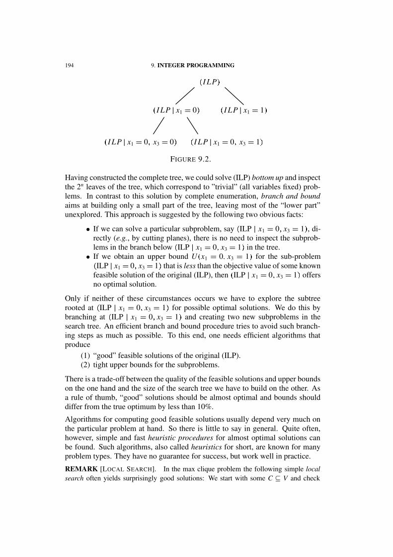
194 9. INTEGER PROGRAMMING
� I LP | x1 = 0 � x3 = 1 �� I LP | x1 = 0 � x3 = 0 �
� I LP | x1 = 0 �
� I LP �
� I LP | x1 = 1 �
FIGURE 9.2.
Having constructed the complete tree, we could solve (ILP) bottom up and inspectthe 2n leaves of the tree, which correspond to ”trivial” (all variables fixed) prob-lems. In contrast to this solution by complete enumeration, branch and boundaims at building only a small part of the tree, leaving most of the “lower part”unexplored. This approach is suggested by the following two obvious facts:
• If we can solve a particular subproblem, say � ILP | x1 = 0 � x3 = 1 � , di-rectly (e.g., by cutting planes), there is no need to inspect the subprob-lems in the branch below � ILP | x1 = 0 � x3 = 1 � in the tree.• If we obtain an upper bound U � x1 = 0 � x3 = 1 � for the sub-problem� ILP | x1 = 0 � x3 = 1 � that is less than the objective value of some known
feasible solution of the original (ILP), then � ILP | x1 = 0 � x3 = 1 � offersno optimal solution.
Only if neither of these circumstances occurs we have to explore the subtreerooted at � ILP | x1 = 0 � x3 = 1 � for possible optimal solutions. We do this bybranching at � ILP | x1 = 0 � x3 = 1 � and creating two new subproblems in thesearch tree. An efficient branch and bound procedure tries to avoid such branch-ing steps as much as possible. To this end, one needs efficient algorithms thatproduce
(1) “good” feasible solutions of the original (ILP).(2) tight upper bounds for the subproblems.
There is a trade-off between the quality of the feasible solutions and upper boundson the one hand and the size of the search tree we have to build on the other. Asa rule of thumb, “good” solutions should be almost optimal and bounds shoulddiffer from the true optimum by less than 10%.
Algorithms for computing good feasible solutions usually depend very much onthe particular problem at hand. So there is little to say in general. Quite often,however, simple and fast heuristic procedures for almost optimal solutions canbe found. Such algorithms, also called heuristics for short, are known for manyproblem types. They have no guarantee for success, but work well in practice.
REMARK [LOCAL SEARCH]. In the max clique problem the following simple localsearch often yields surprisingly good solutions: We start with some C ⊆ V and check
9.5. LAGRANGIAN RELAXATION 195
whether the removal of some node i ∈ C or the addition of some node j �∈ C yields animprovement. If so, we add (delete) the corresponding node and continue this way untilno such improvement is possible (in which case we stop with the current local optimumC ⊆ V). This procedure may be repeated with different initial solutions C ⊆ V .
Computing good upper bounds is usually more difficult. Often, one just solvesthe corresponding LP-relaxations. If these are too weak, one can try to improvethem by adding cutting planes as outlined in Section 9.3 . An alternative is toobtain upper bounds from Lagrangian relaxation (see Section 9.5 below).
Search and Branching Strategies. For the practical execution of a branch andbound algorithm, one needs to specify how one should proceed. Suppose, forexample, that we are in a situation as indicated in Figure 9.2, i.e., that we havebranched from (ILP) on variable x1 and from � ILP | x1 = 0 � on variable x3. Wethen face the question which subproblem to consider next, either � ILP | x1 = 1 �or one of the subproblems of � ILP | x1 = 0 � . There are two possible (extremal)strategies: We either always go to one of the “lowest” (most restricted) subprob-lems or to one of the “highest” (least restricted) subproblems. The latter strategy,choosing � ILP | x1 = 1 � in our case, is called breadth first search while the for-mer strategy is referred to as depth first search, as it moves down the search treeas fast as possible.
A second question concerns the way of branching itself. If LP-relaxation or cut-ting planes are used for computing upper bounds, we obtain a fractional optimumx∗ each time we try to solve a subproblem. A commonly used branching rulethen branches on the most fractional x∗i . In the case of (0 � 1)-variables, this rulebranches on the variable xi for which x∗i is closest to 1 6 2. In concrete applications,we have perhaps an idea about the “relevance” of the variables. We may then al-ternatively decide to branch on the most relevant variable xi. Advanced softwarepackages for integer programming allow the user to specify the branching processand support various upper bounding techniques.
REMARK. The branch and bound approach can easily be extended to general integerproblems. Instead of fixing a variable xi to either 0 or 1, we may restrict it to xi ≤ % i orxi ≥ % i+ 1 for suitable % i ∈ Z. Indeed, the general idea is to partition a given subprobleminto a number of (possibly more than just two) subproblems of similar type.
9.5. Lagrangian RelaxationIn Section 5.1, Lagrangian relaxation was introduced as a means for calculatingupper bounds for optimization problems. Thereby, one “relaxes” (dualizes) some(in)equality constraints by adding them to the objective function using Lagrangianmultipliers y≥ 0 (in case of inequality constraints) to obtain an upper bound L � y � .The crucial question is which constraints to dualize. The more constraints aredualized, the weaker the bound becomes. On the other hand, dualizing moreconstraints facilitates the computation of L � y � . There is a trade-off between the
196 9. INTEGER PROGRAMMING
quality of the bounds we obtain and the effort necessary for their computation.Generally, one would dualize only the “difficult” constraints, i.e., those that aredifficult to deal with directly (see Section 9.5.2 for an example).
Held and Karp [39] were the first to apply the idea of Lagrangian relaxation tointeger linear programs. Assume that we are given an integer program as
(9.26) max {cTx | Ax ≤ b � Bx ≤ d � x ∈ Zn}for given integral matrices A � B and vectors b � c � d and let z∗I P be the optimumvalue of (9.26). Dualizing the constraints Ax − b ≤ 0 with multipliers u ≥ 0yields the upper bound
L � u � = max {cTx− uT � Ax− b � | Bx ≤ d � x ∈ Zn}(9.27)= uTb+max { � cT − uTA � x | Bx ≤ d � x ∈ Zn}
and thus the Lagrangian dual problem
(9.28) z∗D = minu≥0
L � u � �
EX. 9.13. Show that L � u � is an upper bound on z∗I P for every u ≥ 0.
It is instructive to compare (9.28) with the linear programming relaxation
(9.29) z∗LP = max {cTx | Ax ≤ b � Bx ≤ d} �which we obtain by dropping the integrality constraint x ∈ Zn. We find that La-grangian relaxation approximates the true optimum z∗I P at least as well:
THEOREM 9.2. z∗I P ≤ z∗D ≤ z∗LP.
Proof. The first inequality is clear (cf. Ex. 9.13). The second one follows fromthe fact that the Lagrangian dual of a linear program equals the linear program-ming dual. Formally, we may derive the second inequality by applying linearprogramming duality twice:
z∗D = minu≥0
L � u �= min
u≥0[uTb+max
x{ � cT − uTA � x | Bx ≤ d � x ∈ Zn}]
≤ minu≥0
[uTb+maxx{ � cT − uTA � x | Bx ≤ d}]
= minu≥0
[uTb+minv{dTv | vTB = cT − uTA � v ≥ 0}]
= minu + v {uTb+ vTd | uTA+ vTB = cT � u ≥ 0 � v ≥ 0}
= maxx{cTx | Ax ≤ b � Bx ≤ d} = z∗LP �
�
9.5. LAGRANGIAN RELAXATION 197
REMARK. As the proof of Theorem 9.2 shows, z∗D = z∗LP holds if and only if the inte-grality constraint x ∈ Zn is redundant in the Lagrangian dual problem defining z∗D. In thiscase, the Lagrangian dual is said to have the integrality property (cf. Geoffrion [29]).
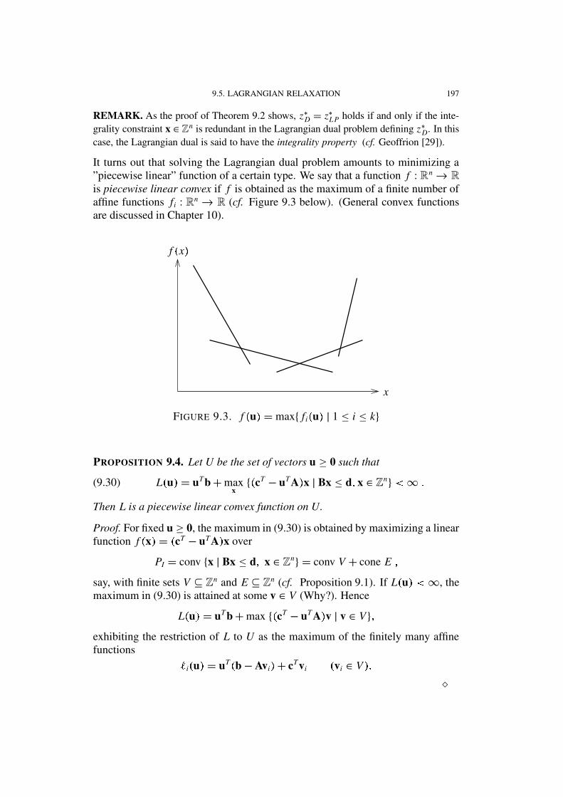
It turns out that solving the Lagrangian dual problem amounts to minimizing a”piecewise linear” function of a certain type. We say that a function f : Rn→ R
is piecewise linear convex if f is obtained as the maximum of a finite number ofaffine functions fi : Rn → R (cf. Figure 9.3 below). (General convex functionsare discussed in Chapter 10).
x
f � x �
FIGURE 9.3. f � u � = max{ fi � u � | 1 ≤ i ≤ k}
PROPOSITION 9.4. Let U be the set of vectors u ≥ 0 such that
(9.30) L � u � = uTb+maxx{ � cT − uTA � x | Bx ≤ d � x ∈ Zn} � ∞ �
Then L is a piecewise linear convex function on U.
Proof. For fixed u ≥ 0, the maximum in (9.30) is obtained by maximizing a linearfunction f � x � = � cT − uTA � x over
PI = conv {x | Bx ≤ d � x ∈ Zn} = conv V + cone E �say, with finite sets V ⊆ Zn and E ⊆ Zn (cf. Proposition 9.1). If L � u � � ∞, themaximum in (9.30) is attained at some v ∈ V (Why?). Hence
L � u � = uTb+max { � cT − uTA � v | v ∈ V} �exhibiting the restriction of L to U as the maximum of the finitely many affinefunctions
R i � u � = uT � b−Avi � + cTvi � vi ∈ V � ��
198 9. INTEGER PROGRAMMING
9.5.1. Solving the Lagrangian Dual. After these structural investigations,let us address the problem of computing (at least approximately) the best possibleupper bound L � u∗ � and solving the Lagrangian dual
z∗D = minu≥0
L � u � �To this end, we assume that we can evaluate (i.e., efficiently solve) for any givenu ≥ 0:
(9.31) L � u � = max {cTx− uT � Ax− b � | Bx ≤ d � x ∈ Zn} �REMARK. In practice this means that the constraints we dualize (Ax ≤ b) have to bechosen appropriately so that the resulting L � u � is easy to evaluate (otherwise we obvi-ously cannot expect to solve the problem min L � u � )Suppose x ∈ Zn is an optimal solution of (9.31). We then seek some u ≥ 0 suchthat L � u � � L � u � . Since x is a feasible solution of the maximization problem in(9.31), L � u � � L � u � implies
(9.32) cTx− uT � Ax− b � ≤ L � u � � L � u � = cTx− uT � Ax− b �and hence � u− u � T � Ax− b � � 0 �The Subgradient Method. The preceding argument suggests to try a vector u =u+∆u with
∆u = u− u = � � Ax− b �for some small step size
� � 0.
Of course, we also want to have u = u +∆u ≥ 0. So we simply replace anynegative component by 0, i.e., we project the resulting vector u onto the set Rm
+ offeasible multipliers and obtain
(9.33) u = max{0 � u+ � � Ax− b � } (componentwise) �REMARK. This procedure appears intuitively reasonable: As our step size � is small,a negative component can only occur if ui ≈ 0 and Ai·x � bi. This means that we donot need to enforce the constraint Ai·x ≤ bi by assigning a large penalty (Lagrangianmultiplier) to it. Consequently, we try ui = 0.
The above procedure is the subgradient method (cf. also Section 5.2.3) for solv-ing the Lagrangian dual: We start with some u0 ≥ 0 and compute a sequenceu1 � u2 � ����� by iterating the above step with step sizes
�1 � � 2 � ����� .
The appropriate choice of the step size�
i is a delicate problem – both in theoryand in practice. A basic result states that convergence takes place (in the sense ofTheorem 11.6) provided
limi→∞
�i = 0 and
∞∑
i=0
�i =∞ �

9.5. LAGRANGIAN RELAXATION 199
9.5.2. Max Clique Revisited. How could Lagrangian relaxation be appliedto the max clique problem? The first (and most crucial) step is to establish anappropriate ILP formulation of the max clique problem. This formulation shouldbe such that dualizing a suitable subset of constraints yields upper bounds that arereasonably tight and efficiently computable. A bit of experimenting reveals ouroriginal formulation (9.7) resp. (9.21) to be inadequate. Below, we shall derivean alternative formulation that turns out to work better.
We start by passing from the underlying complete graph Kn = � V � E � to the com-plete directed graph Dn = � V � A � , replacing each edge e = � i � j � ∈ E by twooppositely directed arcs � i � j � ∈ A and � j � i � ∈ A. To avoid confusion with the no-tation, we will always indicate whether a pair � i � j � is considered as an ordered orunordered pair and write � i � j � ∈ A or � i � j � ∈ E, resp. With each arc � i � j � ∈ A, weassociate a binary variable yi j. The original edge weights de � e ∈ E � are equallyreplaced by arc weights qi j = q ji = de 6 2 (e = � i � j � ∈ E).
The original ILP formulation (9.7) can now be equivalently replaced by
(9.34)
max cTx+ qTy s � t �� 1 � xi + x j − 12 � yi j + y ji � ≤ 1 � i � j � ∈ E� 2 � yi j − y ji = 0 � i � j � ∈ E� 3 � yi j − xi ≤ 0 � i � j � ∈ A� 4 � x ∈ {0 � 1}V � y ∈ {0 � 1}A
REMARK. (9.34) is a “directed version” of (9.7). The cliques (subsets) C ⊆ V are nowin one-to-one correspondence with the feasible solutions of (9.34), namely the vertex-arcincidence vectors � x y � ∈ {0 1}V∪A, defined by xi = 1 if i ∈ C and yi j = 1 if i j ∈ C.
The directed version (9.34) offers the following advantage over the formulation(9.7): After dualizing constraints (1) and (2) in (9.34), the remaining constraints(3) and (4) imply no “dependence” between different nodes i and j (i.e., y i j = 1implies xi = 1 but not x j = 1) . The resulting Lagrangian relaxation can thereforebe solved quite easily (cf. Ex. 9.14).
EX. 9.14. Using Lagrangian multipliers u ∈ RE+ for dualizing constraints (1) and unre-
stricted multipliers v ∈ RE for dualizing the equality constraints (2) in (9.34), one obtains
L � u v � = max cTx+ qTy+∑
� i + j � ∈E
ui j(1− xi − x j +
12� yi j + y ji
� )+ ∑
� i + j � ∈E
ai j � yi j − y ji
�subject to (3)–(4) from (9.34) .
So for given u ∈ RE+ and v ∈ RE, computing L � u v � amounts to solving a problem of the
following type (with suitable c ∈ RV and q ∈ RA):
max cTx+ qTy subject to (3)–(4) from (9.34)
Show: A problem of the latter type is easy to solve because the constraints (3)–(4) implyno “dependence” between different nodes i and j.(Hint: For i ∈ V, let Pi = { j ∈ V | qi j & 0}. Set xi = 1 if ci +
∑j∈Pi
qi j & 0.)
200 9. INTEGER PROGRAMMING
Unfortunately, the Lagrangian bounds we obtain from the dualization of the con-straints (1) and (2) in (9.34) are too weak to be useful in practice. To derive tighterbounds, we want to add more constraints to (9.34) while keeping the enlarged sys-tem still efficiently solvable after dualizing constraints (1) and (2). It turns out thatone can add “directed versions” (cf. below) of the clique inequalities (9.23) andthe i-clique inequalities (9.25) for S = V without complicating things too much.The resulting formulation of the max clique problem is
(9.35)
max cTx+ qTy s.t.� 1 � xi + x j − 1
2 � yi j + y ji � ≤ 1 � i � j � ∈ E� 2 � yi j − y ji = 0 � i � j � ∈ E� 3 � yi j − xi ≤ 0 � i � j � ∈ A� 4 � 2 1 x � V � − y � V � ≤ 1��?1 + 1 � 1 = 1 � ����� � n� 5 � 2 1 y �J� + � i ��� − y � V � − 1��?1 − 1 � xi ≤ 0 i ∈ V� 6 � x ∈ {0 � 1}V � y ∈ {0 � 1}Awhere, in constraints (4) and (5), we used the straightforward extension of ourgeneral shorthand notation:
y � V � = ∑
� i + j � ∈A
yi j and y �J� + � i ��� =∑j 6=i
yi j �Constraints (4) and (5) are “directed versions” of the original clique and i-cliqueinequalities (9.23) and (9.25).
EX. 9.15. Show that every incidence vector � x y � ∈ RV∪A of a set (clique) C ⊆ Vsatisfies the constraints in (9.35). (Hint: Section 9.3)
To dualize constraints (1) and (2) in (9.35), we introduce Lagrangian multipliersu ∈ RE
+ for the inequality constraints (1) and unrestricted multipliers v ∈ RE forthe equality constraints (2). So we obtain for L � u � v � the expression
max cTx+ qTy+∑
� i + j � ∈E
ui j(1− xi − x j +
12� yi j + y ji � )+ ∑
� i + j � ∈E
_i j � yi j − y ji �
subject to (3)–(6) from (9.35) �Given u ∈ RE
+ and v ∈ RE, the computation of L � u � v � amounts to solving a prob-lem of the following type (for suitable c ∈ RV and q ∈ RA):
max cTx+ qTy subject to (3)–(6) from (9.35)(9.36)
The integer linear program (9.36) appears to be more difficult, but can still besolved quickly.
For p = 0 � ����� � n, we determine the best solution satisfying x � V � = p as follows:For p = 0, set x = y = 0. Given p ≥ 1, we choose for each i ∈ V the p − 1most profitable arcs in � + � i � , i.e., those with the highest q-values. Suppose theirq-values sum up to qi for i ∈ V . We then let xi = 1 for the p largest values ofci + qi. If xi = 1, we let yi j = 1 for the p− 1 most profitable arcs in � + � i � .
9.5. LAGRANGIAN RELAXATION 201
The optimal solution is then the best we found for p = 0 � ����� � n. This followsfrom
LEMMA 9.2. Let � x � y � ∈ {0 � 1}V∪A. Then � x � y � is a feasible solution of (9.36) ifand only if there exists some p ∈ {0 � ����� � n} such that
� i � x � V � = p and � ii � y �J� + � i ��� ={
p− 1 if xi = 1 � i ∈ V �0 if xi = 0
Proof. Assume first that � x � y � satisfies (i) and (ii). Then � x � y � satisfies the con-straints (3) and (6) of (9.35). Constraint (4) reduces to
(4’) 2 1 p− p � p− 1 � ≤ 1��?1 + 1 � ,which holds for all 1¦� p ∈ Z since �?1 − p � 2 + �v1 − p � ≥ 0. Constraint (5) iscertainly satisfied if xi = 0 (due to (ii)). For xi = 1, constraint (5) becomes
2 1�� p− 1 � − p � p− 1 � ≤ 1��?1 − 1 � �which is (4’) again.
Conversely, assume that � x � y � is feasible for (9.36) and let p = x � V � =∑i∈V xi.Consider the constraints (5) of (9.36) for those i with xi = 1. Adding the corre-sponding inequalities for any 1 , we find
2 1 y � V � − py � V � − p 1��v1 − 1 � ≤ 0 �Taking 1 = p, we conclude y � V � ≤ p � p− 1 � �On the other hand, letting 1 = p in (4), we have
2p2 − y � V � ≤ p � p+ 1 � and hence y � V � ≥ p � p− 1 � �which proves y � V � = p � p − 1 � . Substituting the latter equality into (5) (with1 = p) and dividing by p, we deduce for i ∈ V with xi = 1:
2y �J� + � i ��� ≤ � p− 1 � + � p− 1 � xi = 2 � p− 1 � �In view of constraint (3) in (9.35), we thus have the inequalities
y �J� + � i ��� ≤{
p− 1 if xi = 10 if xi = 0.
Since y � V � = p � p− 1 � , actually equality must hold.�
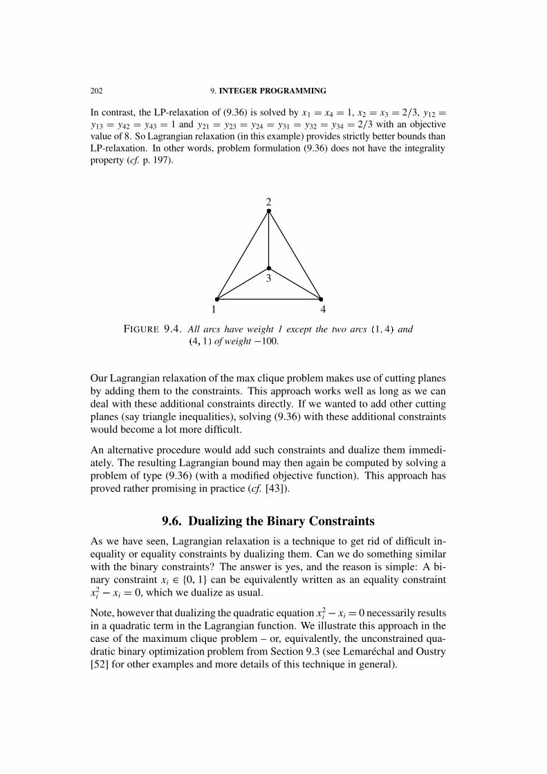
EX. 9.16. The Lagrangian bounds L � u v � we obtain when solving (9.36) as explainedabove are generally better than the bound produced by the LP-relaxation of (9.36). Con-sider, for example, the complete directed graph D4 = � V A � with c = 0 ∈ RV and sym-metric arc weights qi j = q ji as indicated in Figure 9.4 below.An optimum integral solution of (9.36) can be obtained as follows: Choose any set C ⊆ Vwith |C| = 3. Set xi = 1 if i ∈ C. Furthermore, for each i ∈ C choose two arcs in g + � i �with weight qi j = 1. Set yi j = 1 on these two arcs. This solution guarantees an objectivefunction value qTy = 6 (so the duality gap is zero).
202 9. INTEGER PROGRAMMING
In contrast, the LP-relaxation of (9.36) is solved by x1 = x4 = 1, x2 = x3 = 2 � 3, y12 =y13 = y42 = y43 = 1 and y21 = y23 = y24 = y31 = y32 = y34 = 2 � 3 with an objectivevalue of 8. So Lagrangian relaxation (in this example) provides strictly better bounds thanLP-relaxation. In other words, problem formulation (9.36) does not have the integralityproperty (cf. p. 197).
1
2
3
4
FIGURE 9.4. All arcs have weight 1 except the two arcs � 1 4 � and� 4 1 � of weight −100.
Our Lagrangian relaxation of the max clique problem makes use of cutting planesby adding them to the constraints. This approach works well as long as we candeal with these additional constraints directly. If we wanted to add other cuttingplanes (say triangle inequalities), solving (9.36) with these additional constraintswould become a lot more difficult.
An alternative procedure would add such constraints and dualize them immedi-ately. The resulting Lagrangian bound may then again be computed by solving aproblem of type (9.36) (with a modified objective function). This approach hasproved rather promising in practice (cf. [43]).
9.6. Dualizing the Binary ConstraintsAs we have seen, Lagrangian relaxation is a technique to get rid of difficult in-equality or equality constraints by dualizing them. Can we do something similarwith the binary constraints? The answer is yes, and the reason is simple: A bi-nary constraint xi ∈ {0 � 1} can be equivalently written as an equality constraintx2
i − xi = 0, which we dualize as usual.
Note, however that dualizing the quadratic equation x2i − xi = 0 necessarily results
in a quadratic term in the Lagrangian function. We illustrate this approach in thecase of the maximum clique problem – or, equivalently, the unconstrained qua-dratic binary optimization problem from Section 9.3 (see Lemarechal and Oustry[52] for other examples and more details of this technique in general).
9.6. DUALIZING THE BINARY CONSTRAINTS 203
Let Q ∈ Rn×n be a symmetric matrix and reconsider the unconstrained quadraticboolean problem
(9.37) max {xTQx | x ∈ {0 � 1}n} �Dualizing the constraints x2
i − xi = 0 with Lagrangian multipliers ui ∈ R, weobtain the Lagrangian bound
(9.38) L � u � = maxx∈Rn
xTQx+∑
i
ui � x2i − xi � �
Letting U ∈ Rn×n denote the diagonal matrix with diagonal u ∈ Rn, we can write
(9.39) L � u � = maxx
xT � Q+U � x− uTx �Evaluating L � u � amounts to solving the unconstrained quadratic optimizationproblem (9.39). Ex. 9.17 shows how to accomplish this.
EX. 9.17. For fixed u ∈ Rn, consider the function
f � x � = xT � Q+U � x− uTx Show: If x � Q+U � x & 0 holds for some x ∈ Rn, then f has no finite maximum.Assume that xT � Q+U � x ≤ 0 always holds (i.e., Q+U is negative semidefinite). Show:x is optimal for f if and only if ∇ f � x � = 2xT � Q+U � − uT = 0T . (Hint: Section 10.3).So f has a finite maximum if and only if Q+U is negative semidefinite and ∇ f � x � = 0T
has a solution. The maximum is attained in each x ∈ Rn satisfying 2 � Q+U � x= u, whichimplies
L � u � = maxx
f � x � = 12
xTu− uTx = −12
uTx The Lagrangian dual minu L � u � is called the semidefinite relaxation of the primal(9.37), as it can be reformulated as follows (with u ∈ Rn, r ∈ R):
minu
L � u � = minu + r {r | L � u � ≤ r}
= minu + r {r | xT � Q+U � x− uTx ≤ r ∀x ∈ Rn}
= minu + r {r | � 1 � xT �
[−r − 1
2uT
− 12u � Q+U �
](1x
)≤ 0 ∀ x ∈ Rn}
= minu + r { r |
[−r − 1
2uT
− 12u � Q+U �
]is negative semidefinite} �
Only the last step needs further explanation, which is given in Ex. 9.18 below.
EX. 9.18. Show for any S ∈ R � n+1 � × � n+1 � :� 1 xT � S(1
x
)≤ 0 for all x ∈ Rn ⇐⇒ zT Sz ≤ 0 for all z ∈ Rn+1.
204 9. INTEGER PROGRAMMING
Our reformulation of the Lagrangian dual via
minu
L � u � = minr+ u r s � t � Sr + u =
[−r − 1
2uT
− 12u � Q+U �
]� 0 �(9.40)
is a special case of a semidefinite program (optimizing a linear objective underlinear and semidefinite constraints, see also Section12.6).REMARK. To understand how (and why) problem (9.40) can be solved at least approx-imately, consider the following “cutting plane approach”: We first replace the conditionof semidefiniteness for S = Sr + u by a finite number of linear inequalities
(9.41) aT Sa ≤ 0 � a ∈ A �for some finite set A ⊆ Rn+1. Note that, for each fixed a ∈ A, the inequality aT Sa ≤ 0 isa linear inequality with variables r and u.We then minimize r subject to constraints (9.41). If the solution provides us with r and usuch that Sr+ u is negative semidefinite, we have found a solution. Otherwise, if aTSa & 0holds for some a ∈ Rn+1, we add a to A (i.e., we add a violated inequality) and solve themodified problem etc. (Note that we can check whether S = Sr + u is negative semidefinitewith the Diagonalization algorithm from Section 2.1. This also provides us with a suitablevector a in case S is not negative semidefinite.)The theoretical aspects of this approach will be discussed in the context of the ellipsoidmethod in Section 10.6. In practice, analogues of the interior point method for linearprograms (cf. Chapter 6) solve semidefinite programs more efficiently.
We want to emphasize that the approach of dualizing the binary constraints in ageneral integer program
max cTx s.t. Ax ≤ b � x ∈ {0 � 1}nis limited. If we dualize only the binary constraints x2
i − xi = 0 using Lagrangianmultipliers ui ∈ R, the Lagrangian function becomes
L � u � = max xTUx+ � c− u � Tx s.t. Ax ≤ b �In contrast to (9.38), this is a quadratic optimization problem with inequality con-straints, which is in general difficult (NP-hard, cf. Section 8.3).