Integer Programming : Theory and Practice

INTEGERPROGR AMMING

Theory and Practice

OPS_SeriesPage 8/19/05 10:25 AM Page 1

The Operations Research Series

Series Editor: A. Ravi RavindranDept. of Industrial & Manufacturing Engineering

The Pennsylvania State University, USA

Operations Research: A Practical ApproachMichael W. Carter and Camille C. Price

Operations Research Calculations HandbookDennis Blumenfeld

Integer Programming: Theory and PracticeJohn K. Karlof

Forthcoming Titles

Applied Nonlinear Optimization ModelingJanos D. Pinter

Operations Research and Management Science HandbookA. Ravi Ravindran

A CRC title, part of the Taylor & Francis imprint, a member of theTaylor & Francis Group, the academic division of T&F Informa plc.

INTEGERPROGR AMMING

Edited by John K. Karlof

Boca Raton London New York

Theory and Practice

Published in 2006 byCRC PressTaylor & Francis Group 6000 Broken Sound Parkway NW, Suite 300Boca Raton, FL 33487-2742

© 2006 by Taylor & Francis Group, LLCCRC Press is an imprint of Taylor & Francis Group

No claim to original U.S. Government worksPrinted in the United States of America on acid-free paper10 9 8 7 6 5 4 3 2 1

International Standard Book Number-10: 0-8493-1914-5 (Hardcover) International Standard Book Number-13: 978-0-8493-1914-3 (Hardcover) Library of Congress Card Number 2005041912

This book contains information obtained from authentic and highly regarded sources. Reprinted material isquoted with permission, and sources are indicated. A wide variety of references are listed. Reasonable effortshave been made to publish reliable data and information, but the author and the publisher cannot assumeresponsibility for the validity of all materials or for the consequences of their use.

No part of this book may be reprinted, reproduced, transmitted, or utilized in any form by any electronic,mechanical, or other means, now known or hereafter invented, including photocopying, microfilming, andrecording, or in any information storage or retrieval system, without written permission from the publishers.

For permission to photocopy or use material electronically from this work, please access www.copyright.com(http://www.copyright.com/) or contact the Copyright Clearance Center, Inc. (CCC) 222 Rosewood Drive,Danvers, MA 01923, 978-750-8400. CCC is a not-for-profit organization that provides licenses and registrationfor a variety of users. For organizations that have been granted a photocopy license by the CCC, a separatesystem of payment has been arranged.

Trademark Notice: Product or corporate names may be trademarks or registered trademarks, and are used onlyfor identification and explanation without intent to infringe.

Library of Congress Cataloging-in-Publication Data

Integer programming : theory and practice / edited by John K. Karlof. p. cm.

ISBN 0-8493-1914-5 (alk. paper)1. Integer programming. I. Karlof, John K.

T57.74.I547 2005519.7'7--dc22 2005041912

Visit the Taylor & Francis Web site at http://www.taylorandfrancis.com

and the CRC Press Web site at http://www.crcpress.com

Taylor & Francis Group is the Academic Division of T&F Informa plc.

1914_Discl.fm Page 1 Thursday, August 18, 2005 8:51 AM

P1: shibuAugust 23, 2005 10:15 1914 1914˙C000

Preface

Integer programming is a rich and fertile field of applications and theory.This book contains a varied selection of both. I have purposely includedapplications and theory that are usually not found in contributed books inthe hope that the book will appeal to a wide variety of readers. Each of thechapters was invited and refereed. I want to thank the contributors as well asthe referees, who took great care in reviewing each submitted chapter.

The Boolean optimization problem (BOOP) is based on logical expressionsin prepositional first-order logic, with a profit associated with variables hav-ing a true (or false) value subject to these variables making a logical expressiontrue (or false). BOOP represents a large class of binary optimization modelsthat include weighted versions of set covering, graph stability, set partition-ing, and maximum-satisfiability problems. In Chapter 1, Lars Hvattum, ArneLøkketangen, and Fred Glover describe new constructive and iterative searchmethods for solving the BOOP.

Duan Li, Xiaoling Sun, and Jun Wang report recent developments inChapter 2 on convergent Lagrangian techniques that use objective level-cutand domain-cut methods to solve separable nonlinear integer-programmingproblems. The optimal solution to the Lagrangian-relaxation problem doesnot necessarily solve the original problem, even for linear or convex integer-programming problems. This circumstance is the duality gap. The idea of thenew cutting methods is based on the observation that the duality gap can beeliminated by reshaping the perturbation function. Thus, the optimal solutioncan be exposed to the convex hull of the revised perturbation function, whichguarantees the convergence of the Lagrangian method on the revised domain.

Robert Nauss discusses the generalized assignment problem (GAP) inChapter 3. The GAP is concerned with assigning m agents to M tasks sothat the assignment costs are minimized, each task is assigned to exactly oneagent, and resource limitations for each agent are enforced. The GAP may beformulated as a binary-integer linear-programming problem. The problemcan be very difficult to solve with as few as 35 agents and tasks. A special-purpose branch-and-bound algorithm that utilizes a number of tools suchas Lagrangian relaxation, subgradient optimization, lifted cover cuts, logicalfeasibility testing, and specialized feasible-solution generators is presented.

In Chapter 4, Ted Ralphs and Matthew Galati discuss the use of decom-position methods to obtain bounds on the optimal value of solutions tointeger linear-programming problems. Let P be the convex hull of feasiblesolutions. Most bounding procedures are based on the generation of a polyhe-dral approximation to P. The most common approximation is the continuous

P1: shibuAugust 23, 2005 10:15 1914 1914˙C000

approximation. Traditional dynamic procedures for augmenting the continu-ous approximation fall generally into cutting-plane methods and methodsthat dynamically generate extreme points to improve the approximation.Ralphs and Galati describe the principle of decomposition and its applica-tion in the traditional setting. They extend the traditional framework to showhow the cutting-plane method can be integrated with either the Dantzig-Wolfemethod or the Lagrangian method to generate improved bounds. They intro-duce a new concept called structured separation and show how it can be usedin a decomposition framework. Software implementation is also discussed.

Chapter 5 contains models and solution algorithms for the reschedulingof airlines that result from the temporary closure of airports. ShangyaoYan and Chung-Gee Lin consider the operations of a multiple fleet withone-stop and nonstop flights when a single airport is temporally closed,most often because of weather. A basic model is first constructed as a mul-tiple time-space network, from which several strategic network models aredeveloped for scheduling. These network models are formulated as purenetwork-flow problems, network-flow problems with side constraints, ormultiple-commodity network-flow problems. The first are solved by use ofthe network-simplex method, and the others are solved by application of aLagrangian relaxation-based algorithm. The models are shown to be usefulin actual operations by tests on the operations of a major airline.

Chapter 6 and Chapter 7 deal with the determination of an optimal mixof self-owned and chartered vessels of different types that are needed totransport a product. Chapter 6 considers transportation between a singlesource and a single destination, and Chapter 7 considers multiple sourcesto various destinations. Hanif Sherali and Salem Al-Yakoob develop integer-programming models to determine an optimal fleet mix and schedule. Thenew models are solved by application of an optimization package and arecompared to an ad hoc scheduling procedure that simulates how schedulesare generated by a major petroleum corporation.

Chapter 8 presents an application of integer programming that involves thecapture, storage, and transmission of large quantities of data collected duringa variety of possible testing scenarios that might involve military ground ve-hicles, cars, medical applications, large equipment, missiles, or aircraft. Theparticular application that this chapter focuses on is testing military aircraft. Alarge amount of data relating to parameters such as speed, altitude, mechan-ical stress, and pressure is collected. Typically, several hundred or possiblythousands of parameters are continuously sampled during the flight, with asubset of these transmitted to a ground station. The parameters to be trans-mitted are multiplexed into a data structure called a data cycle map, a sequenceof digital words. Data cycle maps are constructed subject to certain regula-tions. One of the most constraining features of the data cycle map constructionprocess is that each parameter must appear periodically within the map. InChapter 8, David Panton, Maria John, and Andrew Mason show how a set-packing integer-programming model may be used to find data cycle mapconstructions that are feasible and efficient.

P1: shibuAugust 23, 2005 10:15 1914 1914˙C000

Govind Daruka and Udatta Palekar consider in Chapter 9 the problem ofdetermining the assortment of products that must be carried by the stores in aretail chain to maximize profit. They develop an integer linear-programmingmodel to solve this problem. The model considers sales forecasts and con-strains the assortments on the basis of available space, desired inventoryturns, advertising restrictions, and other product-specific restrictions. The re-sulting model is solved by use of a column-generation approach. The modeland algorithm were implemented for a large retail chain and have been suc-cessfully used for several years.

Chapter 10 contains an overview of noncommercial software tools for thesolution of mixed-integer linear programs (MILP). Jeff Linderoth and TedRalphs first review solution methodologies for MILP, and then present anoverview of the available software, including detailed descriptions of eightpublicly available software packages. Each package is categorized as a black-box solver, a callable library, a solver framework, or some combination ofthese. The distinguishing features of all eight packages are fully described.The chapter concludes with case studies that illustrate the use of two of thesolver frameworks to develop custom solvers for specific problem classes andwith benchmarking of the six black-box solvers.

P1: shibuAugust 23, 2005 10:15 1914 1914˙C000

P1: shibuAugust 23, 2005 10:15 1914 1914˙C000

The Editor

John Karlof grew up in upstate New York and graduated from The State Uni-versity of New York, Oswego, in 1968 with a B.A. in mathematics. He re-ceived M.A. (1970) and Ph.D. (1973) degrees from the University of Colorado,Boulder, in mathematics. He attended The State University of New York,Stony Brook, in 1981 and received an M.S. in operations research. Dr. Karlofwas professor of mathematics at the University of Nebraska at Omaha from1974 to 1984 and is currently professor of mathematics and graduate coordina-tor at the University of North Carolina, Wilmington, where he has been since1984. His research interests include coding theory, job scheduling, and mathe-matical programming. He has published several papers and directed masterstheses in these areas. In his spare time, Dr. Karlof enjoys racing and cruisingon his 30-foot sailboat, Epsilon, in coastal Carolina.

P1: shibuAugust 23, 2005 10:15 1914 1914˙C000

P1: shibuAugust 23, 2005 10:15 1914 1914˙C000

Contributors

Govind P. Daruka Department of Mechanical and Industrial Engineering,University of Illinois, Urbana, Illinois

Matthew V. Galati Analytical Solutions — Operations R&D, SAS Institute,Cary, North Carolina

Fred Glover Leeds School of Business, University of Colorado, Boulder,Colorado

Lars M. Hvattum Molde University College, Molde, Norway

Maria John Center for Industrial and Applied Mathematics, University ofSouth Australia, Mawson Lakes, South Australia

Duan Li Department of Systems Engineering and Engineering Manage-ment, The Chinese University of Hong Kong, Hong Kong, People’s Re-public of China

Chung-Gee Lin Department of Business Mathematics, Soochow University,Taipei, Taiwan

Jeffrey T. Linderoth Department of Industrial and Systems Engineering,Lehigh University, Bethlehem, Pennsylvania

Arne Løkketangen Molde University College, Molde, Norway

Andrew Mason Department of Engineering Science, University of Auck-land, Auckland, New Zealand

Robert M. Nauss College of Business Administration, University ofMissouri, St. Louis, Missouri

Udatta S. Palekar Department of Mechanical and Industrial Engineering,University of Illinois, Urbana, Illinois

David Panton Center for Industrial and Applied Mathematics, Universityof South Australia, Mawson Lakes, South Australia

P1: shibuAugust 23, 2005 10:15 1914 1914˙C000

Ted K. Ralphs Department of Industrial and Systems Engineering, LehighUniversity, Bethlehem, Pennsylvania

Hanif D. Sherali Department of Industrial and Systems Engineering,Virginia Polytechnic Institute and State University, Blacksburg, Virginia

Xiaoling Sun Department of Mathematics, Shanghai University, Shanghai,People’s Republic of China

Jun Wang Department of Systems Engineering and Engineering Manage-ment, The Chinese University of Hong Kong, Hong Kong, People’s Repub-lic of China

Salem M. Al-Yakoob Department of Mathematics and Computer Science,Kuwait University, Kuwait City, Kuwait

Shangyao Yan Department of Civil Engineering, National Central Univer-sity, Chungli, Taiwan

Referees

Kurt Brethauer Operations and Decision Technologies Department, KelleySchool of Business, Indiana University, Bloomington, Indiana, U.S.

Yaw Chang Department of Mathematics and Statistics, University of NorthCarolina Wilmington, U.S.

Marco Dorigo Iridia, Universite’ Libre de Bruxelles, Belgium

John Forrest IBM, T. J. Watson Research Center, Yorktown Heights, NewYork, U.S.

Lou Hafer School of Computing Science, Simon Fraser University, Burnaby,British Columbia, Canada

Tabitha James Department of Business Information Technology, VirginiaPolytechnic Institute and State University, Blacksburg, Virginia, U.S.

Charles Jones

P1: shibuAugust 23, 2005 10:15 1914 1914˙C000

Andrew Lim Department of Industrial Engineering and Engineering Man-agement, Hong Kong University of Science and Technology, Hong Kong

Tassos Perakis Department of Naval Architecture and Marine Engineering,University of Michigan, Ann Arbor, Michigan, U.S.

David Ronen College of Business Administration, University of Missouri —St. Louis, U.S.

Matthew Tenhuisen Department of Mathematics and Statistics, Universityof North Carolina Wilmington, U.S.

Dusan Teodorovic Department of Civil and Environmental Engineering,Virginia Polytechnic Institute and State University, Blacksburg, Virginia,U.S.

Joris van de Klundert Department of Mathematics, Maastricht University,Maastricht, The Netherlands

Mutsunori Yagiura Department of Applied Mathematics and Physics,Kyoto University, Kyoto, Japan

P1: shibuAugust 23, 2005 10:15 1914 1914˙C000

P1: shibuAugust 23, 2005 10:15 1914 1914˙C000

Contents

1 New Heuristics and Adaptive Memory Proceduresfor Boolean Optimization Problems . . . . . . . . . . . . . . . . . . . . . . . . . . . . . . . . 1Lars M. Hvattum, Arne Løkketangen, and Fred Glover

2 Convergent Lagrangian Methods for SeparableNonlinear Integer Programming:Objective Level Cut and Domain Cut Methods . . . . . . . . . . . . . . . . . . . .19Duan Li, Xiaoling Sun, and Jun Wang

3 The Generalized Assignment Problem . . . . . . . . . . . . . . . . . . . . . . . . . . . . .39Robert M. Nauss

4 Decomposition in Integer Linear Programming . . . . . . . . . . . . . . . . . . . .57Ted K. Ralphs and Matthew V. Galati

5 Airline Scheduling Models and Solution Algorithmsfor the Temporary Closure of Airports . . . . . . . . . . . . . . . . . . . . . . . . . . . .111Shangyao Yan and Chung-Gee Lin

6 Determining an Optimal Fleet Mix and Schedules:Part I — Single Source and Destination . . . . . . . . . . . . . . . . . . . . . . . . . . .137Hanif D. Sherali and Salem M. Al-Yakoob

7 Determining an Optimal Fleet Mix and Schedules:Part II — Multiple Sources and Destinations,and the Option of Leasing Transshipment Depots . . . . . . . . . . . . . . . . 167Hanif D. Sherali and Salem M. Al-Yakoob

8 An Integer Programming Model for the Optimizationof Data Cycle Maps . . . . . . . . . . . . . . . . . . . . . . . . . . . . . . . . . . . . . . . . . . . . . . . 195David Panton, Maria John, and Andrew Mason

9 Application of Column Generation Techniquesto Retail Assortment Planning . . . . . . . . . . . . . . . . . . . . . . . . . . . . . . . . . . . . 221Govind P. Daruka and Udatta S. Palekar

P1: shibuAugust 23, 2005 10:15 1914 1914˙C000

10 Noncommercial Software for Mixed-IntegerLinear Programming . . . . . . . . . . . . . . . . . . . . . . . . . . . . . . . . . . . . . . . . . . . . . .253Jeffrey T. Linderoth and Ted K. Ralphs

Index . . . . . . . . . . . . . . . . . . . . . . . . . . . . . . . . . . . . . . . . . . . . . . . . . . . . . . . . . . . . . . . . . . 305

P1: shibu/Vijay

August 8, 2005 10:7 1914 1914˙C001

1New Heuristics and Adaptive MemoryProcedures for Boolean OptimizationProblems

Lars M. Hvattum, Arne Løkketangen, and Fred Glover

CONTENTS

1.1 Introduction . . . . . . . . . . . . . . . . . . . . . . . . . . . . . . . . . 21.2 Problem Formulation and Search Basics . . . . . . . . . . . . . . . . . 2

1.2.1 Problem Formulation . . . . . . . . . . . . . . . . . . . . . . . . 21.2.2 Local Search Basics . . . . . . . . . . . . . . . . . . . . . . . . . 31.2.3 Move Evaluation Function . . . . . . . . . . . . . . . . . . . . . 4

1.3 Local Search Improvements . . . . . . . . . . . . . . . . . . . . . . . . 41.3.1 Adaptive Clause Weights . . . . . . . . . . . . . . . . . . . . . 51.3.2 Probabilistic Move Acceptance . . . . . . . . . . . . . . . . . . 5

1.4 Constructive Methods . . . . . . . . . . . . . . . . . . . . . . . . . . . 61.4.1 PAM–Persistent Attractiveness Measure . . . . . . . . . . . . . 61.4.2 MCV–Marginal Conditional Validity . . . . . . . . . . . . . . . 71.4.3 A Comparison with GRASP . . . . . . . . . . . . . . . . . . . . 8

1.5 Weighted Maximum Satisfiability . . . . . . . . . . . . . . . . . . . . . 81.6 Computational Results . . . . . . . . . . . . . . . . . . . . . . . . . . . 9

1.6.1 Effect of Adaptive Clause Weights . . . . . . . . . . . . . . . . 91.6.2 Effect of Probabilistic Move Acceptance . . . . . . . . . . . . 101.6.3 PAM and MCV . . . . . . . . . . . . . . . . . . . . . . . . . . 101.6.4 Comparison with GRASP . . . . . . . . . . . . . . . . . . . . 121.6.5 Results for Weighted Maximum Satisfiability . . . . . . . . . 131.6.6 Performance Profiles . . . . . . . . . . . . . . . . . . . . . . . 15

1.7 Conclusions . . . . . . . . . . . . . . . . . . . . . . . . . . . . . . . . 16References . . . . . . . . . . . . . . . . . . . . . . . . . . . . . . . . . . . . 17

1

P1: shibu/Vijay

August 8, 2005 10:7 1914 1914˙C001

2 Integer Programming: Theory and Practice

1.1 Introduction

The Boolean Optimization Problem (BOOP) represents a large class of binaryoptimization models, including weighted versions of Set Covering, GraphStability, Set Partitioning, and Maximum Satisfiability problems. These prob-lems are all NP-hard, and exact (provably convergent) optimization methodsencounter severe performance difficulties in these particular applications,being dominated by heuristic search methods even for moderately sizedproblem instances.

Previous heuristic work on this problem is mainly by Davoine, Hammer,and Vizvari [2], employing a greedy heuristic based on pseudo-boolean func-tions. Hvattum, Løkketangen, and Glover [11] describe simple iterativeheuristic methods for solving BOOP, starting from random initial solutions.Although equipped with no long-term mechanism apart from a randomrestart procedure, they obtain very good results compared to the work byDavoine, Hammer, and Vizvari, and also by an even greater margin whencompared to CPLEX and XPRESS/MP on the larger problems.

The remainder of this chapter is organized as follows. Section 1.2 providesBOOP problem formulations and details of previous work. Section 1.3 de-scribes new local search mechanisms, designed to diversify the search, whileSection 1.4 describes our new constructive methods. In Section 1.5 we addressthe Weighted Maximum Satisfiability problem (W-MAX_SAT), and show howto transform it into a BOOP formulation framework. Computational resultsare given in Section 1.6, followed by the conclusions in Section 1.7.

1.2 Problem Formulation and Search Basics

1.2.1 Problem Formulation

The Boolean Optimization Problem (BOOP), first formulated in Davoine,Hammer, and Vizvari [2], is based on logical expressions in prepositional,first-order logic, with an extra cost (or profit) associated with the variableshaving a true (or false) value. One formulation can be (assuming maximization)

Max z =N∑

i=1

(ci |xi = true/false)

such that

(x) = (x1, . . . , xN) =

truefalse

where (x) is the logical expression, and N the number of variables. Thesolution to this problem is the set of truth value assignments to the xi variablesthat yields the highest objective function value z, while satisfying the logical

P1: shibu/Vijay

August 8, 2005 10:7 1914 1914˙C001

New Heuristics and Adaptive Memory 3

expression. The logical expression can in general be arbitrary, but we restrictourselves to formulations in conjunctive normal form, CNF. (The disjunctivenormal form can be obtained by a simple transformation.) Informally, a BOOPcan be regarded as a satisfiability problem (SAT) with an objective functionadded on. For more information on SAT, see, for example, Cook [1], and Du,Gu, and Pardalos [4].

Applying simple transformations described in Hvattum, Løkketangen, andGlover [11], we get the following model by splitting each xi into its true andfalse component yi and yi#:

Max z =N∑

i=1

ci yi

s.t.

Dy ≥ 1yi + yi# = 1

where D is the 0-1 matrix obtained by substituting the y’s for the xi ’s. The lastconstraint is handled implicitly in the search heuristics we introduce.

1.2.2 Local Search Basics

To better understand the mechanisms described in this chapter, some back-ground from previous work is helpful. Further details can be found inHvattum, Løkketangen, and Glover [11], whereas an introduction to tabusearch can be found in, e.g., Glover and Laguna [10]. The basic strategy of theearlier work includes the following features:

• The starting solution (or starting point) is based on a random assign-ment to the variables. This solution may be primally infeasible, andhence the search must be able to move in infeasible space.

• A move is the flip of a variable by assigning the opposite value (i.e.,change 1 → 0 or 0 → 1).

• The search neighborhood is the full set of possible flips, with a neigh-borhood size of N, the number of variables.

• Move evaluation is based on both the change in objective functionvalue, and the change in amount of infeasibility.

• The move selection is greedy (i.e., take the best move according to themove evaluation).

• Simple randomized tabu tenure and a new best aspiration criterionare used.

• A random restart is applied after a certain number of moves, todiversify the search.

• The stopping criterion is a simple time limit.

P1: shibu/Vijay

August 8, 2005 10:7 1914 1914˙C001


The manner in which we incorporate these features, and add new ones toour current method, is sketched in the following sections.

1.2.3 Move Evaluation Function

The move evaluation function, FMi , has two components. The first is thechange in objective function value. The cost coefficients, ci , are initially nor-malized to lie in the range (0,1). This means that the change in objectivefunction value per move, zi , is in the range (−1, +1).

The second component is the change in the number of violated clauses(or constraint rows), for the flipping of each variable. This number, Vi willusually be a small positive or negative integer. For a different way to handleinfeasible solutions, see Løkketangen and Glover [12].

These two components are combined to balance the considerations of ob-taining solutions that are feasible and that have a good objective functionvalue. The relative emphasis between the two components is changed dy-namically to focus the search in the vicinity of the feasibility boundary, usingthe following move evaluation function:

FMi = Vi + w ∗ zi

The value of w, the adaptive component, is initially set to 1. It is adjusted aftereach move so that:

• If the current solution is feasible: w = w + winc

• If the current solution is not feasible, and w > 1: w = w − wdec

The effect of this adaptation is to induce a strategic oscillation around the fea-sibility boundary. A different approach appears in Glover and Kochenberger[9], where the oscillation is coupled with the use of a critical event memory,forcing the search into new areas.

1.3 Local Search Improvements

The simple local search described in Hvattum, Løkketangen, and Glover [11]relies on a sophisticated adaptive move evaluation scheme for achieving thetype of balance between feasibility and objective function quality previouslydescribed. From their computational results, however, it is evident that forthe larger test cases a better form of diversification than random restart isneeded to be able to explore larger parts of the search space.

The extra mechanisms come at a cost. There is a tradeoff between the gainsprovided by improved search guidance or diversification, and the associatedcomputational effort to perform the extra calculations and to maintain theauxiliary data structures. In the current setting, the additional mechanisms

P1: shibu/Vijay

August 8, 2005 10:7 1914 1914˙C001


reduce the number of search iterations done in a given amount of computa-tional time.

We have implemented two processes for diversification: Adaptive ClauseWeighting, and Probabilistic Move Acceptance.

1.3.1 Adaptive Clause Weights

In the basic local search scheme, all violated clauses (i.e., constraint rows) con-tribute the same amount to the move evaluation function, FMi , as describedin Section 1.2.3. However, some of the clauses will be more difficult to satisfythan others, and should be given more emphasis. We achieve this by attach-ing a separate weight, CW, to each clause. Previous work on adaptive clauseweights can be found in Løkketangen and Glover [13].

All clauses start with CW = 1. The weight is updated only after iterationswhere a clause becomes violated, at which point the weight of the newlyviolated clause is incremented by a small amount, CW. To prevent clauseweights from growing prohibitively large, they are renormalized by dividingall the clause weights by a constant CWDIV, whenever one weight becomesgreater than some CWLIM.

Such a procedure constitutes a long-time learning approach. The moveevaluation function drives the search out of the feasible region to seek solu-tions with high objective function quality in nearby infeasible space. Havingadaptive clause weights helps the search to better adapt to the infeasibilityborder of the search space, thus enabling the search to cross back over the bor-der to find different, and better, feasible solutions. As shown in Section 1.6.1,the tradeoff between the extra time taken to update the weights, and theresulting improved search guidance pays the greatest dividends for the largerproblems.

1.3.2 Probabilistic Move Acceptance

In every iteration the search method generates a list that identifies a subset ofpossible moves to execute, and the best move from this list is selected. Usuallythis best equates with best move evaluation value. But the move evaluation func-tion is rather myopic, only looking at the local neighborhood, and we modifyit by using recency and frequency measures as proposed in tabu search. (See,e.g., Glover and Laguna [10] and Gendreau [6]).

In a sorted list of possible moves, the presumably best moves will be atthe front of the list, but not necessarily in strict order. A simplified variant ofthis principle from Glover [7] is also employed in GRASP, where the chosenmove is randomly selected among the top half of the moves (see Feo andResende [5]).

We use this approach by selecting randomly from the top of the list, but ina way biased toward the moves having the highest evaluations. This is calledProbabilistic Move Acceptance, PMA, as described in Løkketangen and Glover[12]. The selection method is as follows:

P1: shibu/Vijay

August 8, 2005 10:7 1914 1914˙C001


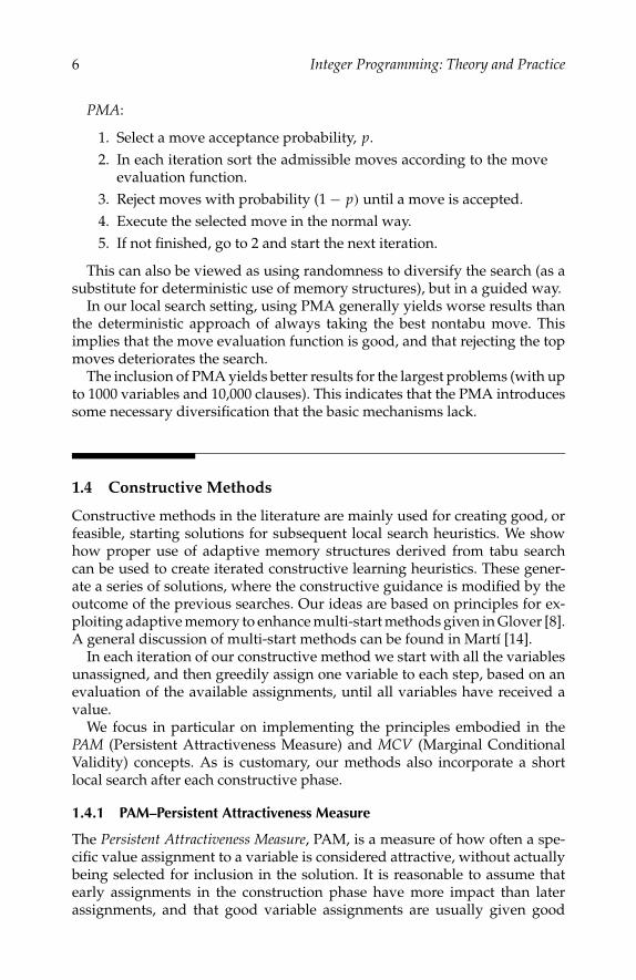
PMA:

1. Select a move acceptance probability, p.2. In each iteration sort the admissible moves according to the move

evaluation function.3. Reject moves with probability (1 − p) until a move is accepted.4. Execute the selected move in the normal way.5. If not finished, go to 2 and start the next iteration.

This can also be viewed as using randomness to diversify the search (as asubstitute for deterministic use of memory structures), but in a guided way.

In our local search setting, using PMA generally yields worse results thanthe deterministic approach of always taking the best nontabu move. Thisimplies that the move evaluation function is good, and that rejecting the topmoves deteriorates the search.

The inclusion of PMA yields better results for the largest problems (with upto 1000 variables and 10,000 clauses). This indicates that the PMA introducessome necessary diversification that the basic mechanisms lack.

1.4 Constructive Methods

Constructive methods in the literature are mainly used for creating good, orfeasible, starting solutions for subsequent local search heuristics. We showhow proper use of adaptive memory structures derived from tabu searchcan be used to create iterated constructive learning heuristics. These gener-ate a series of solutions, where the constructive guidance is modified by theoutcome of the previous searches. Our ideas are based on principles for ex-ploiting adaptive memory to enhance multi-start methods given in Glover [8].A general discussion of multi-start methods can be found in Martı [14].

In each iteration of our constructive method we start with all the variablesunassigned, and then greedily assign one variable to each step, based on anevaluation of the available assignments, until all variables have received avalue.

We focus in particular on implementing the principles embodied in thePAM (Persistent Attractiveness Measure) and MCV (Marginal ConditionalValidity) concepts. As is customary, our methods also incorporate a shortlocal search after each constructive phase.

1.4.1 PAM–Persistent Attractiveness Measure

The Persistent Attractiveness Measure, PAM, is a measure of how often a spe-cific value assignment to a variable is considered attractive, without actuallybeing selected for inclusion in the solution. It is reasonable to assume thatearly assignments in the construction phase have more impact than laterassignments, and that good variable assignments are usually given good

P1: shibu/Vijay

August 8, 2005 10:7 1914 1914˙C001


evaluations. The attractiveness should also increase for a variable assignmentthat is repeatedly ranked high without being chosen.

If we index the assignment steps with s, and the individual rankings in astep with r , we would like the PAM to have the following properties:

PAM(r, s) is decreasing for increasing s (earlier steps are more important)PAM(r, s) is decreasing for increasing r (higher rank is better)

We only calculate PAM for the top ranked moves.The PAM evaluator can be formulated as E(s, r ) = E’(s) + E”(r), where, for

BOOP, we setE′(s) = as∗ − as

andE′′(r) = br∗ − br

where s∗ = N (number of variables) and r is a parameter. The constants aandb are determined experimentally as subsequently described.

The PAM-values corresponding to a given assignment are summed over allthe constructive steps to yield an overall measure of attractiveness for eachpossible assignment.

PAM values for several consecutive constructive runs can be accumulatedin a measure of attractiveness, e.g., by exponential smoothing:

New PAM = (Last PAM + Last Accumulated Total PAM)/2

We thus expand the move evaluation indicated earlier to become:

F(yi(#)) = Vi(#) + w∗(zi(#) + PAMi(#))

The values for the PAM-measure are limited to an interval [0, k], with k chosento match w in some way, again as specified later. The parameter w is updatedas in the local search (see Section 1.2.3), but only after the completion of eachconstructive run.

1.4.2 MCV–Marginal Conditional Validity

The choices made at the beginning of a constructive search are based onless information than later choices, and are thus more likely to be bad. Whenlater choices are made, the problem has been reduced by the earlier choices,and better choices can be made (but in the context of the earlier ones). Laterdecisions are thus likely to make earlier decisions look better. We call this theMarginal Conditional Validity principle.

After the constructive phase we analyze the completed solution to findassignments that should have been different. There are two cases that can beused as a foundation:

1. A variable is true, but there are unsatisfied rows where the negatedvariable is present.

2. A variable is false, but the negated variable is present only in rowsthat would be satisfied even if the variable had been flipped.

P1: shibu/Vijay

August 8, 2005 10:7 1914 1914˙C001


In the first case the opposite value assignment to the variable would possi-bly satisfy more rows, while in the second case we would get an increase inthe objective function value, without violating any new constraints. Each ofthe assignments recognized in this manner is enforced in the start of the nextconstructive run with a given probability p.

1.4.3 A Comparison with GRASP

The Greedy Randomized Adaptive Search Procedure, or GRASP, is a well known,memoryless, constructive heuristic relying heavily on randomization (seeResende, Pitsoulis, and Pardalos, 1997). A constructive run can be followedby a short greedy local search.

We have adapted and implemented GRASP to work for BOOP, for com-parison purposes. We use the same basic objective function value as before,but without any adaptive memory or learning. The only parameter requiredfor GRASP is the proportion of moves to be considered for execution in eachconstructive assignment, called α.

GRASP:

1. Start with all variables unassigned, rate all possible assignments.2. Select an assignment randomly among those who are within α% of

best evaluation.3. When all variables are assigned, possibly do a local search.4. Go to 1, if not finished.

We use time as a stopping criterion, and try three versions of local search (LS):No LS, complete LS, or “steepest ascent” LS.

We also tried to augment GRASP with learning capabilities by introducingthe adaptive component w in the evaluation function, as for our other constr-uctive approach (see Section 1.4.1). Computational results are in Section 1.6.4.

1.5 Weighted Maximum Satisfiability

To support the claim that BOOP can represent many different problem classes,this section outlines how Weighted Maximum Satisfiability problems(W-MAX_SAT) can be easily transformed to BOOP. Section 1.6.5 gives com-putational results for this case, without any effort to specialize our procedureto handle the special structure of this problem.

A W-MAX_SAT instance can informally be regarded as an unsatisfiableinstance of a SAT problem that in addition has weights on the clauses (rows).The objective is then to find a truth assignment that maximizes the sum of theweights on the satisfied clauses. This is similar to BOOP, except that weightsare attached to the clauses rather than the variables. A W-MAX_SAT instancecan be transformed to BOOP by adding a new variable to each clause to

P1: shibu/Vijay

August 8, 2005 10:7 1914 1914˙C001


carry information about weights. The clause weights are transformed to ob-jective function value coefficients for the new variables in the correspondingclauses, while the original n variables will have objective function value co-efficients of 0.

Thus, if the W-MAX_SAT has n variables and m clauses, the BOOP willhave (n + m) variables and m clauses. The number of clauses (rows), m, isoften large compared to the number of variables, n, giving a BOOP encodingfor W-MAX_SAT having many more variables. (In the test instances used inSection 1.6.5 n is 100 and m is 800 to 900, giving 900 to 1000 variables for theBOOP encoding, compared to 100 for W-MAX_SAT.)

As we can see in the computational results Section 1.6.5, our BOOP codecompares favorably to the GRASP heuristic on the same problem instances(Resende, Pitsoulis, and Pardalos [15]), and is only slightly worse than thespecial purpose method of Shang [17] in spite of the fact that no specializationis used in our procedure.

1.6 Computational Results

This section reports the final parameter settings applied to each of the differ-ent methods or mechanisms during testing, as well as overall computationalresults. Section 1.6.6 attempts to compare all the different methods and mech-anisms in a meaningful way.

The same BOOP test cases as used in the previous work (Hvattum, Løkke-tangen, and Glover [11] and Davoine, Hammer, and Vizvari [2]) are usedfor testing. The test-set consists of 5485 instances, ranging in size from 50 to1000 variables, and 200 to 10000 clauses (rows). Results are reported as theaverage of solution values relative to results obtained by Davoine, Hammer,and Vizvari using CPLEX 6.0.

The testing of W-MAX_SAT is based on modifying the unsatisfiable jnh*, asused in Resende, Pitsoulis, and Pardalos [15]. These all have 100 variables and800 to 900 clauses. For preliminary testing to fix parameter values, we selectedthe same three test cases as in Hvattum, Løkketangen, and Glover [11].

1.6.1 Effect of Adaptive Clause Weights

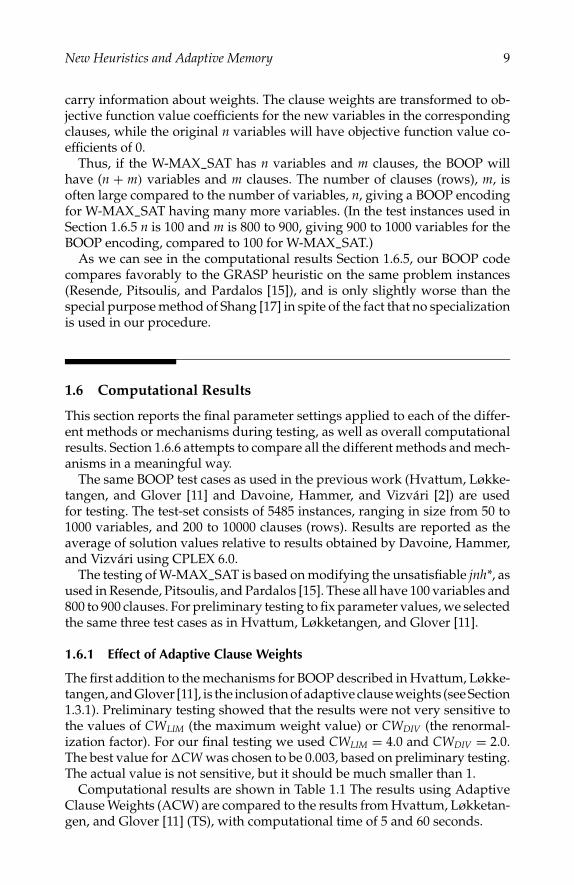
The first addition to the mechanisms for BOOP described in Hvattum, Løkke-tangen, and Glover [11], is the inclusion of adaptive clause weights (see Section1.3.1). Preliminary testing showed that the results were not very sensitive tothe values of CWLIM (the maximum weight value) or CWDIV (the renormal-ization factor). For our final testing we used CWLIM = 4.0 and CWDIV = 2.0.The best value for CW was chosen to be 0.003, based on preliminary testing.The actual value is not sensitive, but it should be much smaller than 1.

Computational results are shown in Table 1.1 The results using AdaptiveClause Weights (ACW) are compared to the results from Hvattum, Løkketan-gen, and Glover [11] (TS), with computational time of 5 and 60 seconds.

P1: shibu/Vijay

August 8, 2005 10:7 1914 1914˙C001


TABLE 1.1

Adaptive Clause WeightsTS 5 TS 60 ACW 5 ACW 60

Classes 1–22 100.001 100.001 100.002 100.002Classes 23–49 101.214 101.215 101.212 101.214Classes 50–54 106.305 106.982 107.628 107.866Classes 55–63 102.463 102.465 102.462 102.464Classes 1–63 101.373 101.427 101.477 101.497

As can be seen, the overall results show an improvement for both the 5second and 60 second cutoff. For classes 55 to 63 the results are slightly inferiorto those of our earlier approach.

1.6.2 Effect of Probabilistic Move Acceptance

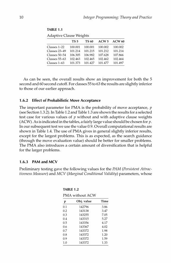
The important parameter for PMA is the probability of move acceptance, p(see Section 1.3.2). In Table 1.2 and Table 1.3 are shown the results for a selectedtest case for various values of p without and with adaptive clause weights(ACW). As is indicated in the tables, a fairly large value should be chosen for p.In our subsequent test we use the value 0.9. Overall computational results areshown in Table 1.4. The use of PMA gives in general slightly inferior results,except for the largest problems. This is as expected, as the search guidance(through the move evaluation value) should be better for smaller problems.The PMA also introduces a certain amount of diversification that is helpfulfor the larger problems.

1.6.3 PAM and MCV

Preliminary testing gave the following values for the PAM (Persistent Attrac-tiveness Measure) and MCV (Marginal Conditional Validity) parameters, whose

TABLE 1.2

PMA without ACWp Obj. value Time

0.1 142796 3.860.2 143138 3.470.3 143255 7.050.4 143315 5.270.5 143356 4.170.6 143367 4.020.7 143372 1.980.8 143372 1.200.9 143372 1.591.0 143372 1.33

P1: shibu/Vijay

August 8, 2005 10:7 1914 1914˙C001


TABLE 1.3

PMA with ACWp Obj. value Time

0.1 142845 5.290.2 143148 6.350.3 143246 6.180.4 143323 5.510.5 143357 6.110.6 143365 4.620.7 143369 2.270.8 143372 1.960.9 143372 1.271.0 143372 0.82

role is sketched in Section 1.4.1 and Section 1.4.2:

a = 2b = 3

r∗ = 4

The PAM-value of each variable assignment is scaled to lie between 0 and 0.3before it is used in the move evaluation function as specified in Section 1.4.1.

Figure 1.1 shows results for the given test case for various values of p, theprobability that determines when to apply the MCV principle. For this testcase the best results are when the MCV principle (p = 0) is not applied. Theresults with p = 0.4 give best results when applying MCV, and this value isused in the computational testing.

Table 1.5 shows the computational results for our constructive learningheuristic applying both PAM and MCV. The column PAM/MCV-NO LS givesthe results when no local search was applied after each constructive run.PAM/MCV-STEEP indicates that a steepest ascent local search was appliedafter each construction, and PAM/MCV-TS 500 indicates that a tabu searchlimited to 500 iterations, as described in Section 1.3.1, was used for improve-ment. All the runs were for 60 seconds. This new constructive method, evenwithout the local search, performs much better than the basic GRASP ap-proach (see Section 1.6.4). The constructive approach without local search (LS)

TABLE 1.4

Results for PMATabu Search PMA w.o. ACW PMA w. ACW

TS 5 TS 60 PMA 5 PMA 60 PMA 5 PMA 60

Classes 1–22 100.001 100.001 99.998 100.000 99.996 99.998Classes 23–49 101.214 101.215 101.205 101.213 101.205 101.211Classes 50–54 106.305 106.982 105.787 106.168 107.438 107.778Classes 55–63 102.463 102.465 102.446 102.463 102.450 102.461Classes 1–63 101.373 101.427 101.324 101.361 101.455 101.487

P1: shibu/Vijay

August 8, 2005 10:7 1914 1914˙C001


MCV parameter

140400

140600140800141000141200

141400141600

0 0.1 0.2 0.3 0.4 0.5 0.6 0.7 0.8 0.9 1

p

ob

ject

ive

valu

e

FIGURE 1.1Values for p for MCV.

also beats the results in Davoine, Hammer, and Vizvari [2] on small instances,and beats, with the addition of a short LS to the constructive approach, theseresults on all the instances.

It seems that when combining the constructive learning heuristic with theTS from Section 1.3.1, most of the benefit comes from the TS. However, themethod PAM/MCV-TS 500 was the only method that finds the optimum of allthe small instances (classes 1 to 22, 5280 instances). In fact, all the optima werefound within 2 seconds. This seems to reflect the trend we have observed forour constructive heuristics, that they are more effective for the smaller prob-lem instances and do not often contribute improved results for the largestproblem instances.

1.6.4 Comparison with GRASP

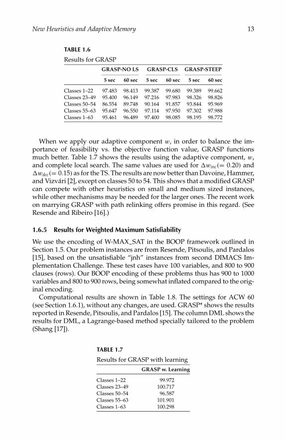
Results for the GRASP heuristic outlined in Section 1.4.3 are shown in Table 1.6,allowing for 5 or 60 seconds search time. A value of α = 0.5 was used. The col-umn GRASP–NO LS shows the results when no local search is applied afterthe constructive phase, and GRASP–CLS shows the results when a complete,recursive, local search is applied. GRASP–STEEP shows the results whensteepest, ascent is used.

These results indicate that GRASP is better than Davoine, Hammer, andVizvari [2] on small instances, but does not scale well for the larger problems.

TABLE 1.5

Results for PAM and MCVPAM/MCV-NO LS PAM/MCV-STEEP PAM/MCV-TS 500

Classes 1–22 99.359 99.780 100.002Classes 23–49 99.571 100.074 101.205Classes 50–54 97.202 98.545 106.778Classes 55–63 99.581 99.942 102.448Classes 1–63 99.310 99.831 101.405

P1: shibu/Vijay

August 8, 2005 10:7 1914 1914˙C001


TABLE 1.6

Results for GRASPGRASP-NO LS GRASP-CLS GRASP-STEEP

5 sec 60 sec 5 sec 60 sec 5 sec 60 sec

Classes 1–22 97.483 98.413 99.387 99.680 99.389 99.662Classes 23–49 95.400 96.149 97.216 97.983 98.326 98.826Classes 50–54 86.554 89.748 90.164 91.857 93.844 95.969Classes 55–63 95.647 96.550 97.114 97.950 97.302 97.988Classes 1–63 95.461 96.489 97.400 98.085 98.195 98.772

When we apply our adaptive component w, in order to balance the im-portance of feasibility vs. the objective function value, GRASP functionsmuch better. Table 1.7 shows the results using the adaptive component, w,and complete local search. The same values are used for winc(= 0.20) andwdec(= 0.15) as for the TS. The results are now better than Davoine, Hammer,and Vizvari [2], except on classes 50 to 54. This shows that a modified GRASPcan compete with other heuristics on small and medium sized instances,while other mechanisms may be needed for the larger ones. The recent workon marrying GRASP with path relinking offers promise in this regard. (SeeResende and Ribeiro [16].)

1.6.5 Results for Weighted Maximum Satisfiability

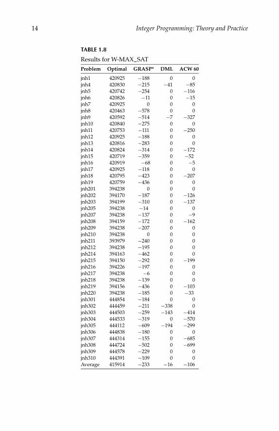
We use the encoding of W-MAX_SAT in the BOOP framework outlined inSection 1.5. Our problem instances are from Resende, Pitsoulis, and Pardalos[15], based on the unsatisfiable “jnh” instances from second DIMACS Im-plementation Challenge. These test cases have 100 variables, and 800 to 900clauses (rows). Our BOOP encoding of these problems thus has 900 to 1000variables and 800 to 900 rows, being somewhat inflated compared to the orig-inal encoding.

Computational results are shown in Table 1.8. The settings for ACW 60(see Section 1.6.1), without any changes, are used. GRASP* shows the resultsreported in Resende, Pitsoulis, and Pardalos [15]. The column DML shows theresults for DML, a Lagrange-based method specially tailored to the problem(Shang [17]).

TABLE 1.7

Results for GRASP with learningGRASP w. Learning

Classes 1–22 99.972Classes 23–49 100.717Classes 50–54 96.587Classes 55–63 101.901Classes 1–63 100.298

P1: shibu/Vijay

August 8, 2005 10:7 1914 1914˙C001


TABLE 1.8

Results for W-MAX_SATProblem Optimal GRASP* DML ACW 60

jnh1 420925 −188 0 0jnh4 420830 −215 −41 −85jnh5 420742 −254 0 −116jnh6 420826 −11 0 −15jnh7 420925 0 0 0jnh8 420463 −578 0 0jnh9 420592 −514 −7 −327jnh10 420840 −275 0 0jnh11 420753 −111 0 −250jnh12 420925 −188 0 0jnh13 420816 −283 0 0jnh14 420824 −314 0 −172jnh15 420719 −359 0 −52jnh16 420919 −68 0 −5jnh17 420925 −118 0 0jnh18 420795 −423 0 −207jnh19 420759 −436 0 0jnh201 394238 0 0 0jnh202 394170 −187 0 −126jnh203 394199 −310 0 −137jnh205 394238 −14 0 0jnh207 394238 −137 0 −9jnh208 394159 −172 0 −162jnh209 394238 −207 0 0jnh210 394238 0 0 0jnh211 393979 −240 0 0jnh212 394238 −195 0 0jnh214 394163 −462 0 0jnh215 394150 −292 0 −199jnh216 394226 −197 0 0jnh217 394238 −6 0 0jnh218 394238 −139 0 0jnh219 394156 −436 0 −103jnh220 394238 −185 0 −33jnh301 444854 −184 0 0jnh302 444459 −211 −338 0jnh303 444503 −259 −143 −414jnh304 444533 −319 0 −570jnh305 444112 −609 −194 −299jnh306 444838 −180 0 0jnh307 444314 −155 0 −685jnh308 444724 −502 0 −699jnh309 444578 −229 0 0jnh310 444391 −109 0 0Average 415914 −233 −16 −106

P1: shibu/Vijay

August 8, 2005 10:7 1914 1914˙C001


Our computational results compare favorably to those of the GRASPheuristic on the same problem instances. Our outcomes are only slightly worsethan those of the special purpose DML method of Shang [17], although weare undertaking to solve the much larger transformed problem and make nouse of any specialization.

1.6.6 Performance Profiles

It is always very difficult to compare different methods based on tables ofcomputational results, unless one method is best on all the tests. We thereforealso compare our methods using the ideas given in Dolan and More [3]. Basedon the time used to find the best solution, we can construct a performanceprofile as follows.

Let P be the set of problem instances, S be the set of solvers, and np bethe number of problems. Define tp,s to be the time used by solver s to solveproblem p. Let

rp,s = tp,s

mintp,s∗|s∗ ∈ Sbe the ratio between the performances of solver s to the best solver on theproblem p. If a solver fails to solve a problem, then set rp,s = rM, where rM ≥rp,s for all p and s.

A measure of the performance of a solver can be given by

ρs (τ ) = 1np

sizep ∈ P|rp,s ≤ τ

where ρs (τ ) is the probability that for solver s, the ratio of performance rp,s iswithin a factor τ of the best ratio. A plot of ρs (τ ) for the different solvers willgive interesting characteristics of the solvers. Please note that ρs (1) gives theproportion of problems where s is winning over the other solvers.

For many of our problem instances the reported solution time is very small,and the solvers report 0. All these instances are removed from this compari-son. This is not necessarily a drawback, as the remaining problems’ instancespresumably are the most interesting ones.

Figure 1.2 shows performance profiles for the following six methods:

• ACW 60 – Tabu Search with adaptive clause weights• TS 60 – Tabu Search without adaptive clause weights• PMA 60 TS – Tabu Search without adaptive clause weights, but

with PMA• CON ACW – Constructive Search, followed by TS• CON LS – Constructive Search, followed by Steepest Ascent• CON – Constructive Search – No LS

The allotted solution times are 60 seconds per problem instance.

P1: shibu/Vijay

August 8, 2005 10:7 1914 1914˙C001


CONCON LSCON ACWPMA 60 TSTS 60ACW 60

T

1

0.9

0.8

0.7

0.6

0.5

0.4

0.3

0.2

0.1

050045040035030025020015010050

FIGURE 1.2Performance profiles.

Of the original 5485 problem instances, 352 were left after removing thosewhere at least one of the solvers reported a solution time of 0 seconds. Ofthese remaining problems there are 299 where not all the solvers find thesame solution value.

As can be seen, the method ACW 60 is the best. It is of interest to note thatwhen solution time is small (less than a factor 40 from the best solver on eachparticular instance), is that CON ACW is better than PMA 60 TS, while forlonger solution times PMA 60 TS is better.

1.7 Conclusions

We have shown the value of certain types of adaptive memory to improvethe performance of heuristics, both iterative and constructive. Our resultscompare very favorably to previous published results, and are significantlybetter than those obtained by exact solvers (XPRESS and CPLEX).

For BOOP, we have achieved the best results by using a tabu search basedheuristic, augmented by an adaptive move evaluation function, and adaptiveclause weights. Very good results are also obtained for constructive heuristicsaugmented by the learning schemes of PAM (Persistent Attractiveness Measure)and MCV (Marginal Conditional Validity).

P1: shibu/Vijay

August 8, 2005 10:7 1914 1914˙C001


We also show that our approach can be applied to Weighted MaximumSatisfiability problems by transforming them into (larger) BOOP problems,and that without specialization to the W-MAX_SAT setting we obtain resultscomparable to those of the better specialized methods from the literature.

References

1. Cook, S. A., The complexity of theorem-proving procedures, in Proc. Third ACMSymp. on Theory of Computing, 1971, 151.

2. Davoine, T., Hammer P. L., and Vizvari, B., A heuristic for Boolean optimizationproblems, J of Heuristics, 9, 229, 2003.

3. Dolan, E. D. and More J. J., Benchmarking optimization software with per-formance profiles, preprint ANL/MCS-P861-1200, Mathematics and ComputerScience Division, Argonne National Laboratory, 2001.

4. Du, D., Gu, J., and Pardalos, P., Eds., Satisfiability Problem: Theory and Applications,DIMACS Series in Discrete Mathematics and Theoretical Computer Science,Vol. 35, AMS, 1997.

5. Feo, T. A. and Resende M. G. C., A probabilistic heuristic for a computationallydifficult set covering problem, Operations Research Letters, 8, 67, 1989.

6. Gendreau, M., An introduction to tabu Search, in Handbook of Metaheuristics,Glover, F. and Kochenberger, G., Eds., Kluwer Academic Publishers, 2003,37.

7. Glover, F., Tabu search — part I, ORSA Journal on Computing, 1, 190, 1989.8. Glover, F., Multi-start and strategic oscillation methods — principles to exploit

adaptive memory, in OR Computing Tools for Modeling, Optimization and Sim-ulation: Interfaces in Computer Science and Operations Research, Laguna, M. andGonzalez-Velarde, J. L., 2000, 1.

9. Glover, F. and Kochenberger, G., Critical event tabu search for multidimensionalknapsack problems, in Meta Heuristics: Theory and Applications, Osman, I. H. andKelly, J. P., Eds., Kluwer Academic Publishers, 1996, 407.

10. Glover, F. and Laguna, M., Tabu Search, Kluwer Academic Publishers, 1997.11. Hvattum, L. M., Løkketangen, A., and Glover, F., Adaptive memory search for

Boolean optimization problems, Discrete Applied Mathematics, 142, 99, 2004.12. Løkketangen, A. and Glover F., Probabilistic move selection in tabu Search for

0/1 mixed integer programming problems, in Metaheuristics: Theory and Appli-cations, Eds.: Osman, I. H. and Kelly, J. P., Eds., Kluwer Academic Publishers,1996, 467.

13. Løkketangen, A. and Glover, F., Surrogate constraint analysis — new heuristicsand learning schemes for satisfiability problems, in Satisfiability Problem: Theoryand Applications, Du, D., Gu, J., and Pardalos, P. M., Eds., DIMACS Series inDiscrete Mathematics and Theoretical Computer Science, Vol. 35, AMS, 1997,pp. 537–572.

14. Martı, R., Multi-start methods, in Handbook of Metaheuristics, Glover, F. andKochenberger, G., Eds., Kluwer Academic Publishers, 2003, 355.

15. Resende, M. G. C., Pitsoulis, L. S., and Pardalos, P. M., Approximate solutionof weighted MAX-SAT problems using GRASP, in Satisfiability Problem: Theoryand Applications, Du, D., Gu, J., and Pardalos, P. M., Eds., DIMACS Series in

P1: shibu/Vijay

August 8, 2005 10:7 1914 1914˙C001


Discrete Mathematics and Theoretical Computer Science, Vol. 35, AMS, 1997,393.

16. Resende, M. G. C. and Ribeiro, C. C., GRASP with path-relinking: recent ad-vances and applications, submitted to Metaheuristics: Progress as Real ProblemSolvers, Ibaraki, T., Nonobe, K., and Yagiura, M., Eds., Springer, 2005.

17. Shang, Y., Global search methods for solving nonlinear optimization prob-lems, Ph.D. Thesis, Dept. of Computer Science, University of Illinois, Urbana-Champaign, 1997.

P1: shibu/Vijay

August 12, 2005 9:48 1914 1914˙C002

2Convergent Lagrangian Methods forSeparable Nonlinear Integer Programming:Objective Level Cut and Domain Cut Methods

Duan Li, Xiaoling Sun, and Jun Wang

CONTENTS

2.1 Introduction . . . . . . . . . . . . . . . . . . . . . . . . . . . . . . . . 192.2 Lagrangian Relaxation, Perturbation Function, and Duality . . . . . 202.3 Objective Level Cut Method . . . . . . . . . . . . . . . . . . . . . . . 252.4 Domain Cut Method . . . . . . . . . . . . . . . . . . . . . . . . . . . 292.5 Numerical Results . . . . . . . . . . . . . . . . . . . . . . . . . . . . 332.6 Summary . . . . . . . . . . . . . . . . . . . . . . . . . . . . . . . . . . 35Acknowledgments . . . . . . . . . . . . . . . . . . . . . . . . . . . . . . . 36References . . . . . . . . . . . . . . . . . . . . . . . . . . . . . . . . . . . . 36

2.1 Introduction

We consider the following general class of separable integer programmingproblems:

(P) min f (x) =n∑

j=1

f j (xj )

s.t. gi (x) =n∑

j=1

gi j (xj ) ≤ bi , i = 1, . . . , m, (2.1)

x ∈ X = X1 × X2 × . . . × Xn,

where all f j s are integer-valued functions, all gijs are real-valued functionsand all Xj s are finite integer sets in R.

Problem (P) has a wide variety of applications, including resource alloca-tion problems and nonlinear knapsack problems. In particular, manufacturing

19

P1: shibu/Vijay

August 12, 2005 9:48 1914 1914˙C002


capacity planning, stratified sampling, production planning, and networkreliability are special cases of (P) (see [2][10][22] and the references therein).

The solution methods for problem (P) and its special cases can be classi-fied into three major categories, dynamic programming ([4][11]), branch-and-bound methods ([2][3][8]), and Lagrangian relaxation methods ([5–7][19])(plus some combinations of branch-and-bound and dynamic programmingmethods [18]). Although dynamic programming is conceptually an ideal so-lution scheme for separable integer programming, the “curse of dimension-ality” prevents its direct application to the multiply constrained cases of (P)

when m is large. The success of branch-and-bound methods based on contin-uous relaxation relies on their ability to identify a global optimal solution tocontinuous relaxation subproblems. Thus, branch-and-bound methods maynot be applicable to (P) when a nonconvexity is presented which is oftenthe case in many applications, e.g., concave integer programming and poly-nomial integer programming. Due to the often existence of a duality gap,Lagrangian relaxation methods in many situations are not used as an exactmethod to find an optimal solution for (P). Developing an efficient solutionscheme for general separable nonlinear integer programming problems in(P) is a challenging task.

Two convergent Lagrangian methods using the objective level cut anddomain cut methods have been recently developed in [14–16] for solvingseparable nonlinear integer programming problems. The purpose of thischapter is to discuss the solution concepts behind these two new methodsin order to give new insights and to stimulate further research results.

2.2 Lagrangian Relaxation, Perturbation Function, and Duality

By associating with each constraint in (P) a nonnegative λi , the Lagrangianrelaxation of (P) is formulated as

(Lλ) d(λ) = minx∈X

L(x, λ) = f (x) +m∑

i=1

λi (gi (x) − bi ), (2.2)

where λ = (λ1, . . . , λm)T ∈ Rm+ and L(x, λ) is called the Lagrangian function

of (P). One of the prominent features of the Lagrangian relaxation problem(Lλ) is that it can be decomposed into n one-dimensional problems:

min f j (xj ) +m∑

i=1

λi gi j (xj ) (2.3)

s.t. xj ∈ Xj .

Notice that (2.3) is a problem of minimizing a univariate function over a finiteinteger set and its optimal solution can be easily identified. Denote the optimal

P1: shibu/Vijay

August 12, 2005 9:48 1914 1914˙C002

Convergent Lagrangian Methods 21

value of problem (Q) as v(Q). Let the feasible region and the optimal valueof (P) be defined as,

S = x ∈ X | gi (x) ≤ bi , i = 1, . . . , m,v(P) = f ∗ = min

x∈Sf (x).

Since d(λ) ≤ f (x) for all x ∈ S and λ ≥ 0, the dual value d(λ) always providesa lower bound for the optimal value of (P) (weak duality):

v(P) = f ∗ ≥ d(λ), ∀λ ≥ 0.

We assume in the sequel that minx∈X f (x) < f ∗, otherwise minx∈X = f ∗ musthold and (P) reduces to an unconstrained integer programming problem. TheLagrangian dual problem of (P) is to search for an optimal multiplier vectorλ∗ ∈ Rm

+ which maximizes d(λ) for all λ ≥ 0:

(D) d(λ∗) = maxλ≥0

d(λ). (2.4)

By weak duality, f ∗ ≥ d(λ∗) holds. The difference f ∗ − d(λ∗) is called the du-ality gap between (P) and (D). Let u be an upper bound of f ∗. We denoteu − d(λ∗) as a duality bound between (P) and (D). It is clear that a dualitybound is always larger than or equal to the duality gap.

If x∗ solves (Lλ∗) with λ∗ ≥ 0, and, in addition, the following conditions aresatisfied:

gi (x∗) ≤ bi , i = 1, 2, . . . , m, (2.5)

λ∗i (gi (x∗) − bi ) = 0, i = 1, 2, . . . , m, (2.6)

then x∗ solves (P) and v(P) = v(D), i.e., the duality gap is zero. In thissituation, the strong Lagrangian duality condition is said to be satisfied.Unfortunately, the strong Lagrangian duality is rarely present in integer pro-gramming, and a nonzero duality gap often exists when the Lagrangianrelaxation method is adopted.

For any vectors x and y ∈ Rm, denote x ≤ y iff xi ≤ yi , i = 1, . . . , m. Afunction h defined on Rm is said to be nonincreasing if for any x and y ∈ Rm,x ≤ y implies h(x) ≥ h(y).

Let g(x) = (g1(x), . . . , gm(x))T and b = (b1, . . . , bm)T . The perturbationfunction of (P) is defined as follows for y ∈ Rm,

w(y) = min f (x) | g(x) ≤ y, x ∈ X, (2.7)

where the domain of w is

Y = y ∈ Rm | there exists x ∈ X such that g(x) ≤ y. (2.8)

It is easy to see that w(g(x)) ≤ f (x) for any x ∈ X and w(b) = f ∗. By the def-inition of the perturbation function in (2.7), w(y) is a nonincreasing function.

P1: shibu/Vijay

August 12, 2005 9:48 1914 1914˙C002


Moreover, since X is a finite set, w is a piecewise constant function over Y.The domain Y can be decomposed as Y = ∪K

k=1Yk , where K is a finite numberand Yk is a subset over which w takes constant value fk :

w(y) = fk , ∀y ∈ Yk, k = 1, . . . , K . (2.9)

For singly constrained cases of (P), i.e., m = 1, Yk has the following form:

Yk =

[ck , ck+1), k = 1, . . . , K − 1,

[ck , +∞), k = K,(2.10)

where c1 = minx∈X g1(x).

For multiply constrained cases of (P), define

cki = minyi | y = (y1, . . . , ym)T ∈ Yk, k = 1, . . . , K , i = 1, . . . , m,C = ck = (ck1, . . . , ckm)T | k = 1, . . . , K ,

c = (ck , fk) | k = 1, . . . , K , = (y, w(y)) | y ∈ Y.

It follows from the definition of w that ck ∈ Yk for k = 1, . . . , K and thusc ⊂ . A point in c is said to be a corner point of the perturbation function w.It is clear that (y, w(y)) ∈ c iff (y, w(y)) ∈ and for any z ∈ Y satisfyingz ≤ y and z = y, w(z) > w(y) holds. For all x ∈ X, the points (g(x), f (x)) areon or above the image of the perturbation function.

A vector λ ∈ Rm is said to be a subgradient of w(·) at y = y if

w(y) ≥ w(y) + λT (y − y), ∀y ∈ Y.

LEMMA 2.1 [17]Let x∗ solve primal problem (P). Then x∗ is a solution to Lagrangian relaxationproblem (L λ) for some λ in Rm

+ iff −λ is a subgradient of w(·) at y = g(x∗).Define the convex envelope function of w to be the greatest convex function

majorized by w:

ψ(y) = maxh(y) | h(y) is convex on Y, h(y) ≤ w(y), ∀y ∈ Y. (2.11)

It can be easily seen that ψ is piecewise linear and nonincreasing on Y andw(y) ≥ ψ(y) for all y ∈ Y. Moreover, by the convexity of ψ we have

ψ(y) = maxλT y + r | λ ∈ Rm, r ∈ R, and λT z + r ≤ w(z), ∀z ∈ Y,

or equivalently,

ψ(y) = max λT y + r (2.12)s.t. λT ck + r ≤ fk , k = 1, . . . , K ,

λ ∈ Rm, r ∈ R.

P1: shibu/Vijay

August 12, 2005 9:48 1914 1914˙C002


For any fixed y ∈ Y, we introduce a dual variable µk ≥ 0 for each constraintλT ck + r ≤ fk , k = 1, . . . , K . Dualizing the linear program (2.12) then yields

ψ(y) = minK∑

k=1

µk fk (2.13)

s.t.K∑

k=1

µkck ≤ y,

K∑i=1

µk = 1, µk ≥ 0, k = 1, . . . , K .

THEOREM 2.1 [15][17]Let (−λ∗, r∗) and µ∗ be optimal solutions to (2.12) and (2.13) with y = b, respec-tively. Then

i. λ∗ is an optimal solution to the dual problem (D) and

ψ(b) = maxλ≥0

d(λ) = d(λ∗). (2.14)

ii. For each k with µ∗k > 0, any x ∈ X satisfying (g(x), f (x)) = (ck , fk)

is an optimal solution to the Lagrangian problem (Lλ∗).

THEOREM 2.2 [17]Let x∗ solve (P). Then, x∗, λ∗ is an optimal primal-dual pair iff the hyperplane givenby w = f (x∗) − (λ∗)T [y − g(x∗)] is a supporting hyperplane at [ f (x∗), g(x∗)] andcontains [ψ(b), b].

Now let us investigate the reasons behind the often failures of the tradi-tional Lagrangian method in finding an exact solution of the primal problem.Consider the following example.

Example 2.1

min f (x) = −2x21 − x2 + 3x2

3

s.t. 5x1 + 3x22 −

√3x3 ≤ 7,

x ∈ X = 0 ≤ xi ≤ 2, xi integer, i = 1, 2, 3.

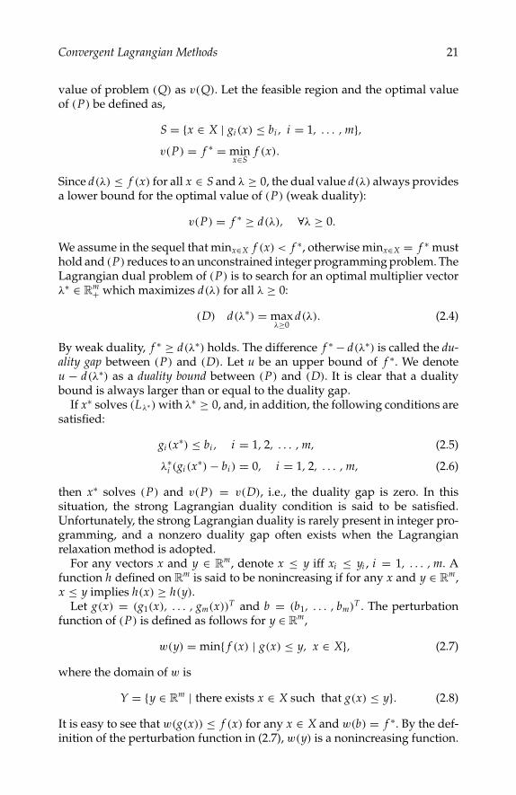
The optimal solution of this example is x∗ = (1, 0, 0)T with f ∗ = f(x∗) = −2.The perturbation function of this problem is illustrated in Figure 2.1. We cansee from Figure 2.1 that point C that corresponds to the optimal solution x∗

“hides” above the convex envelope of the perturbation function and thereforethere does not exist a subgradient of perturbation function w at g(x∗). In otherwords, it is impossible for x∗ to be found by the conventional Lagrangiandual method. The optimal solution to (D) in this example is λ∗ = 0.8 withd(λ∗) = −5.6. Note the solutions to (Lλ∗=0.8) are (0, 0, 0)T and (2, 0, 0)T , nei-ther of which is optimal to the primal problem.

P1: shibu/Vijay

August 12, 2005 9:48 1914 1914˙C002


C

y=7

B1=(10,–8|( 2,0,0)) A1=(0,0|(0,0,0))

C=(5,–2| (1,0,0))

B1

A1

(g(x),f(x)|x)

–5.6

w(y

)

y

10

5

0

–5

–10

2520151050–5

FIGURE 2.1The perturbation function of Example 2.1.

A vector λ∗ ≥ 0 is said to be an optimal generating multiplier vector of (P) ifan optimal solution x∗ to (P) can be generated by solving (Lλ) with λ = λ∗

(see [17]). A pair (x∗, λ∗) is said to be an optimal primal-dual pair of (P) if theoptimal dual solution λ∗ to (D) is an optimal generating multiplier vector foran optimal solution x∗ to (P) (see [17]).

The conventional Lagrangian dual method would fail in two critical situ-ations, both of which have been witnessed in the above example. The firstsituation occurs where no solution of (P) can be generated by problem (Lλ)

for any λ ≥ 0. The second situation occurs where no solution to problem (Lλ∗),with λ∗ being an optimal solution to (D), is a solution to (P).

It is clear that the nonexistence of a linear support at the optimal point leadsto a failure of the traditional Lagrangian method. Recognizing the existence ofa nonlinear support, nonlinear Lagrangian formulations have been proposedin [12][13][17][20][21] to offer a success guarantee for the dual search in gen-erating an optimal solution of the primal integer programming problem. Incontrast to the traditional Lagrangian formulation which is linear with respectto the objective function and constraints, a nonlinear Lagrangian formulationtakes nonlinear forms such as pth power or a logarithmic-exponential formu-lation with respect to the objective function and constraints.

While the nonlinear Lagrangian theory provides a theoretical mechanismto guarantee the success of the dual search, the nonlinear Lagrangian formula-tion does not lead to a decomposability which is the most prominent feature ofthe traditional linear Lagrangian. When the original problem is separable, thenonlinear Lagrangian formulation destroys the original separable structure

P1: shibu/Vijay

August 12, 2005 9:48 1914 1914˙C002


and makes the decomposition impossible. Thus, the computational and im-plementation issue of nonlinear Lagrangian theory in integer programmingremains unsolved since there is no efficient algorithm to solve a general non-separable integer programming problem.

Stimulated by the relationship between the duality gap and the geome-try of the perturbation function, two novel convergent Lagrangian methodsadopting the objective level cut method and the domain cut method haverecently been developed for (P) in [14–16]. They are efficient and convergentLagrangian solution schemes in a sense that they provide an exact solution to(P) while retaining the decomposability of (P) in the solution process. Bothmethods are devised to reshape the perturbation function by adding somecuts such that the duality gap can be reduced. A successive reshaping pro-cess will eventually expose the optimal solution on the convex envelop of arevised perturbation function and thus the success of convergent dual searchcan be guaranteed.

2.3 Objective Level Cut Method

We continue to investigate Example 2.1 to motivate the development of theobjective level cut method [14] [15].

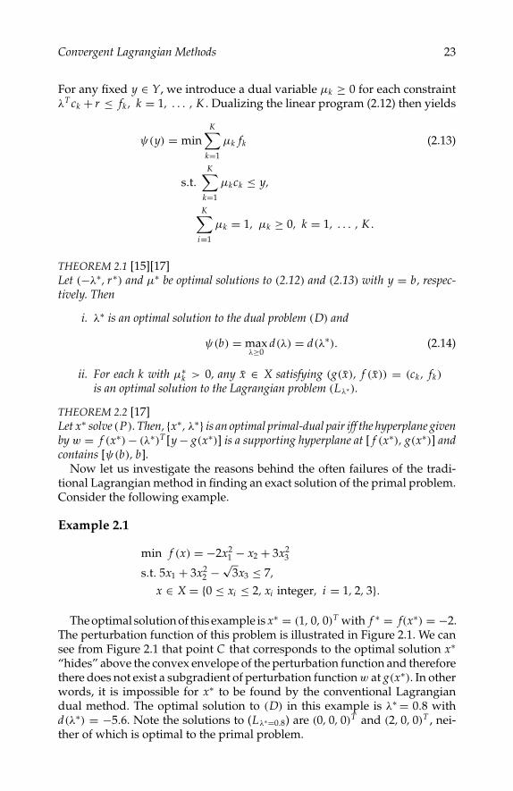
As we observed from Figure 2.1, the optimal point C hides above the convexenvelope of the perturbation and there is no optimal generating vector at C .The duality gap is f (x∗) − d(λ∗) = −2 − (−5.6) = 3.6 and the current dualitybound is 0 − (−5.6) = 5.6 achieved by the traditional Lagrangian method.A key finding is that point C can be exposed to the convex envelope or theconvex hull of the perturbation function by adding an objective cut. As amatter of fact, since A1 corresponds to a feasible solution x0 = (0, 0, 0)T , thefunction value f (x0) = 0 is an upper bound of f ∗. Moreover, by the weakduality, the dual value d(λ∗) = −5.6 is a lower bound of f ∗. Therefore, addingan objective cut of −5.6 ≤ f (x) ≤ 0 to the original problem does not excludethe optimal solution, while the perturbation function will be reshaped dueto the modified feasible region. Since the objective function is integer-valued,we can set a stronger objective cut of −5 ≤ f (x) ≤ −1 after storing the currentbest feasible solution x0 as the incumbent. The modified problem then has thefollowing form:

min f (x) = −2x21 − x2 + 3x2

3 (2.15)

s.t. 5x1 + 3x22 −

√3x3 ≤ 7,

x ∈ X1 = X ∩ x | −5 ≤ f (x) ≤ −1.The perturbation function of (2.15) is shown in Figure 2.2. The optimal dualmultiplier to (2.15) is 0.7593 with dual value −4.0372. Since x1 = (0, 1, 0)T

corresponding to A2 is feasible, the duality bound is now reduced to f (x1) −(−4.0372) = −1 + 4.0372 = 3.0372. Again we can add an objective

P1: shibu/Vijay

August 12, 2005 9:48 1914 1914˙C002


–4.0372

y=7

C

B2

A2

(g(x),f(x)|x)

B2=(8.2679,–5|( 2,0,1))

A2=(3,–1|(0,1,0)) C=(5,–2| (1,0,0))

w(y

)

y

0

–1

–2

–3

–4

–5

–618161412108642

FIGURE 2.2The perturbation function of (2.15).

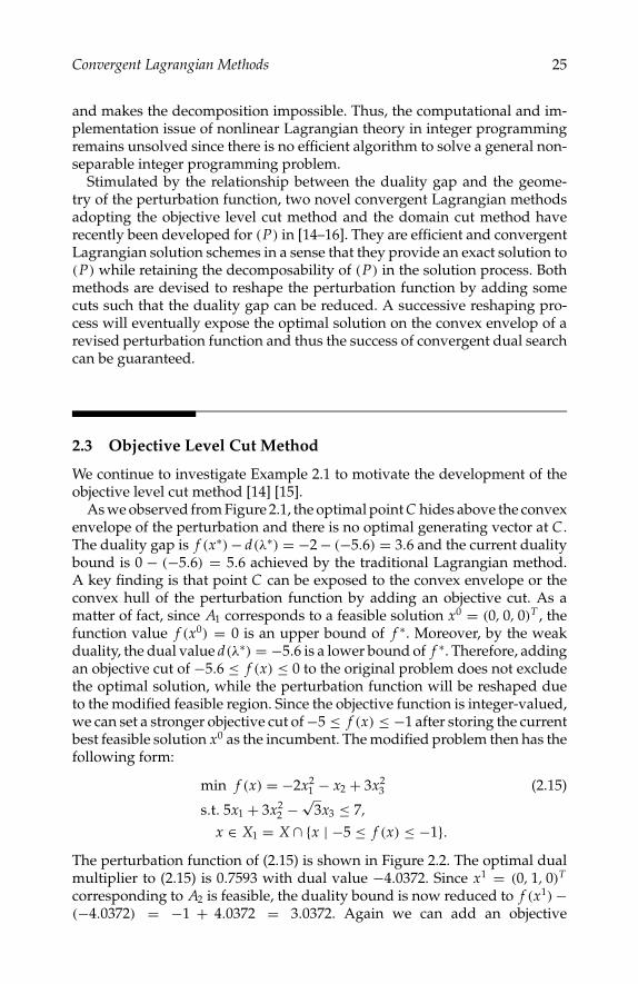
cut −4 ≤ f (x) ≤ f (x1) − 1 = −2 to (2.15) and obtain the following problem:

min f (x) = −2x21 − x2 + 3x2

3 (2.16)

s.t. 5x1 + 3x22 −

√3x3 ≤ 7,

x ∈ X2 = X ∩ x | −4 ≤ f (x) ≤ −2.The perturbation function of (2.16) is shown in Figure 2.3. The optimal dualmultiplier is 0.3333 with dual value −2.6667. Now point C corresponding tox∗ is exposed to the convex hull of the perturbation function and the dualitybound is reduced to f (x∗) − (−2.6667) = −2 + 2.6667 = 0.6667 < 1. Sincethe objective function is integer-valued, we claim that x∗ = (1, 0, 0)T is theoptimal solution to the original problem.

To reduce the duality gap between the Lagrangian dual problem and theprimal problem, we reshape the perturbation function by adding objectivecut to the problem. We start with a lower bound derived from the dual valueby the conventional dual search and an upper bound by a feasible solutiongenerated in the dual search (if any). The updated lower level cut and upperlevel cut are imposed to the program successively such that the duality bound(duality gap) is forced to shrink. Note that there is only one lower bound andupper bound constraint during the whole solution process.

How to solve the relaxation problems of the revised problems such as theLagrangian relaxations of (2.15) and (2.16) is crucial to an efficient implemen-tation of this novel idea. The Lagrangian relaxation of each revised problemis a separable integer programming with a lower bound and upper bound

P1: shibu/Vijay

August 12, 2005 9:48 1914 1914˙C002


–2.6667

y=7

(g(x),f(x)|x)

B3

C

B3=(8,–3|(1,1,0)) C=(5,–2| (1,0,0))

w(y

)

y

–1.5

–2

–2.5

–3

–3.5

–4

–4.51816141210864

FIGURE 2.3The perturbation function of (2.16).

constraint for the objective function. Since the objective function is integer-valued, dynamic programming can be used to search for optimal solutions tothis kind of problems efficiently. Consider the following modified version of(P) by imposing a lower cut l and an upper cut u:

(P(l, u)) min f (x) (2.17)s.t. gi (x) ≤ bi , i = 1, . . . , m,

x ∈ X(l, u) = x ∈ X | l ≤ f (x) ≤ u.It is obvious that (P(l, u)) is equivalent to (P) if l ≤ f ∗ ≤ u. The Lagrangianrelaxation of (P(l, u)) is:

(Lλ(l, u)) d(λ, l, u) = minx∈X(l,u)

L(x, λ). (2.18)

The Lagrangian dual problem of (P(l, u)) is then given as

(D(l, u)) maxλ≥0

d(λ, l, u). (2.19)

Notice that (Lλ(l, u)) can be explicitly written as:

d(λ, l, u) = min

[f (x) +

m∑i=1

λi (gi (x) − bi )

]= min

n∑

j=1

θ j (xj , λ) − α(λ)

(2.20)

s.t. l ≤n∑

j=1

f j (xj ) ≤ u,

x ∈ X,

P1: shibu/Vijay

August 12, 2005 9:48 1914 1914˙C002


where θ j (xj , λ) = f j (xj ) + mi=1λi gi j (xj ) and α(λ) = m

i=1λi bi . It is clear that(Lλ(l, u)) is a separable integer programming problem with a lower boundand upper bound constraint on f (x). By the assumptions in (P), each f j (xj )

is integer-valued for all xj ∈ Xj . Therefore, (Lλ(l, u)) can be efficiently solvedby dynamic programming. Let

sk =k−1∑j=1

f j (xj ), k = 2, . . . , n + 1, (2.21)

with an initial condition of s1 = 0. Then (Lλ(l, u)) can be solved by the fol-lowing dynamic programming formulation:

(DP) min sn+1 +n∑

j=1

[m∑

i=1

λi gi j (xj )

](2.22)

s.t. s j+1 = s j + f j (xj ), j = 1, 2, . . . , n,

s1 = 0,

l ≤ sn+1 ≤ u,

xj ∈ Xj , j = 1, 2, . . . , n.

The state in the above dynamic programming formulation takes finite valuesat each stage.

THEOREM 2.3Let λ∗ be the optimal solution to (D). Denote by T(λ∗) the set of the optimal solu-tions to the Lagrangian problem (Lλ∗). Assume that the duality gap is nonzero, i.e.,d(λ∗) < f ∗. Then

i. There is at least one infeasible solution to (Lλ∗);

ii. min f (x) | x ∈ T(λ∗) \ S ≤ d(λ∗).

Based on Theorem 3, the objective cut is always valid when the duality gapis nonzero. More specifically, in each new cut, some infeasible solution that isthe solution to the previous Lagrangian relaxation problem will be removed,thus raising the dual value in the current iteration.

THEOREM 2.4

i. Let λ∗(l, u) denote the optimal solution to (D(l, u)). The dual optimalvalue d(λ∗(l, u), l, u) is a nondecreasing function of l.

ii. If l ≤ f ∗ ≤ u, then d(λ∗) ≤ d(λ∗(l, u), l, u) ≤ f ∗. Moreover, let σ =max f (x) | f (x) < f ∗, x ∈ X \ S. If σ < l ≤ f ∗, then λ∗(l, u) = 0and d(λ∗(l, u), l, u) = f ∗.

iii. For l < f ∗, we have d(λ∗(l, u), l, u) ≥ l.

The implication of Theorem 4 is clear: The higher the lower cut, the higherthe dual value. The solution process will stop when the duality gap is less than

P1: shibu/Vijay

August 12, 2005 9:48 1914 1914˙C002


one. From Theorem 2.3 and Theorem 2.4, the following result of finite con-vergence is evident.

THEOREM 2.5The objective level cut algorithm either finds an optimal solution of (P) or reports aninfeasibility of (P) in at most u0 − l0 + 1 iterations, where u0 and l0 are the upperand lower bounds generated in the first iteration using the conventional Lagrangianmethod.

Although the objective function is assumed to be integer-valued in theobjective level cut algorithm, a rational objective function can be also handledby multiplying the objective function by the least common multiplier of thedenominators of all coefficients.

2.4 Domain Cut Method

When the objective function in (P) is a nonincreasing function with respectto all xi s and all the constraints are nondecreasing functions with respect toall xi s, problem (P) becomes a nonlinear knapsack problem. The domain cutmethod [14][16] is developed for solving nonlinear knapsack problems. Notethat the assumption of integer-valued objective function is not needed in thedomain cut method.

We illustrate the solution concept of the domain cut method by the follow-ing example.

Example 2.2

min f (x) = −x21 − 1.5x2

s.t. g(x) = 6x1 + x22 ≤ 23,

x ∈ X = x | 1 ≤ xi ≤ 4, xi integer, i = 1, 2.

Note that f is nonincreasing and g is nondecreasing. The optimal solution ofthis example is x∗ = (3, 2)T with f (x∗) = −12.

The domain X and the perturbation function z = w(y) of this example areillustrated in Figure 2.4 and Figure 2.5, respectively. It is easy to check thatthe optimal Lagrangian multiplier is λ∗ = 0.8333 with dual value −15.8333.The duality gap is 3.8333. The Lagrangian problem

minx∈X

[ f (x) + 0.8333(g(x) − 23)]

has a feasible solution x0 = (1, 1)T with f (x0) = −2.5 and an infeasible solutiony0 = (4, 1)T . In Figure 2.5, points A, B, C correspond to x0, y0, and x∗ in(g(x), f (x)) plane, respectively. We observe that if points Aand B are removedfrom the plot of the perturbation function, then the duality gap of the revised

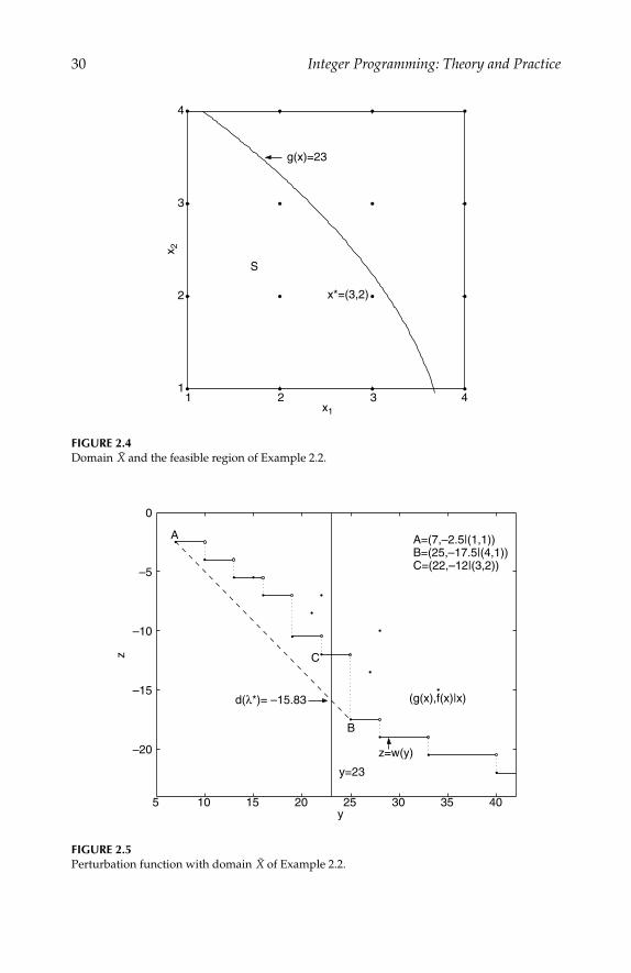
P1: shibu/Vijay

August 12, 2005 9:48 1914 1914˙C002


S

x*=(3,2)

g(x)=23 x 2

x1

4

3

2

14321

FIGURE 2.4Domain X and the feasible region of Example 2.2.

z=w(y)

(g(x),f(x)|x) d(λ*)= –15.83

C

B

A

C=(22,–12|(3,2)) B=(25,–17.5|(4,1))

A=(7,–2.5|(1,1))

y=23

z

y

0

–5

–10

–15

–20

403530252015105

FIGURE 2.5Perturbation function with domain X of Example 2.2.

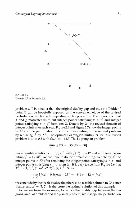
P1: shibu/Vijay

August 12, 2005 9:48 1914 1914˙C002


x2

x13 2

4

3

2 x*=(3,2)

g(x)=23

FIGURE 2.6Domain X1 in Example 2.2.

problem will be smaller than the original duality gap and thus the “hidden”point C can be hopefully exposed on the convex envelope of the revisedperturbation function after repeating such a procedure. The monotonicity off and g motivates us to cut integer points satisfying x ≤ x0 and integerpoints satisfying x ≥ y0 from box X. Denote by X1 the revised domain ofinteger points after such a cut. Figure 2.6 and Figure 2.7 show the integer pointsin X1 and the perturbation function corresponding to the revised problemby replacing X by X1. The optimal Lagrangian multiplier for this revisedproblem is λ∗ = 0.3 with d(λ∗) = −12.3. The Lagrangian problem

minx∈X1

[ f (x) + 0.3(g(x) − 23)]

has a feasible solution x1 = (3, 2)T with f (x1) = −12 and an infeasible so-lution y1 = (3, 3)T . We continue to do the domain cutting. Denote by X2 theinteger points in X1 after removing the integer points satisfying x ≤ x1 andinteger points satisfying x ≥ y1 from X1. It is easy to see from Figure 2.6 thatX2 = (1, 3)T , (1, 4)T , (2, 3)T , (2, 4)T . Since

minx∈X2

[ f (x) + 0.3(g(x) − 23)] = −9.1 > −12 = f (x1),

we conclude by the weak duality that there is no feasible solution in X2 betterthan x1 and x1 = (3, 2)T is therefore the optimal solution of this example.

As we see from the example, to reduce the duality gap between the La-grangian dual problem and the primal problem, we reshape the perturbation

P1: shibu/Vijay

August 12, 2005 9:48 1914 1914˙C002


d(λ*)= –12.3 B

C z=w(y)

(g(x),f(x)|x)

y=23

C=(22,–12|(3,2)) B=(27,–13.5|(3,3))

z

y

0

–2

–4

–6

–8

–10

–12

–14

–16353025201510

FIGURE 2.7Perturbation function with domain X1 of Example 2.2.

function by removing certain points from the domain X. The monotonicity ofthe problem guarantees that an optimal solution either has been found duringthe search or is still in the remaining feasible region after the domain cut.

Let α, β ∈ Zn, where Zn denotes the set of integer points in Rn. Let 〈α, β〉denote the set of integer points in [α, β],

〈α, β〉 =n∏

i=1

〈αi , βi 〉 = 〈α1, β1〉 × 〈α2, β2〉 . . . × 〈αn, βn〉.

We call 〈α, β〉 an integer box. Let l = (l1, . . . , ln)T and u = (u1, . . . , un)

T .Assume that the integer set X in (P) is given by X = 〈l, u〉. If the objectivefunction is nonincreasing and constraints are nondecreasing, we have thefollowing conclusions:

i. If x ∈ 〈l, u〉 is a feasible solution to (P), then for any x ∈ 〈l, x〉, it holdsthat f (x) ≥ f (x).

ii. If y ∈ 〈l, u〉 is an infeasible solution to (P), then any point in 〈y, u〉is infeasible.

Therefore, 〈l, x〉 and 〈y, u〉 can be cut from the 〈l, u〉, without missing anyoptimal solution of (P) after recording the feasible solution x.

A critical issue for an efficient implementation of the domain cut methodis how to characterize the nonbox revised domain after performing a cuttingprocess. In [14][16], the following analytical formulas are derived to describethe revised domain as a union of subboxes.

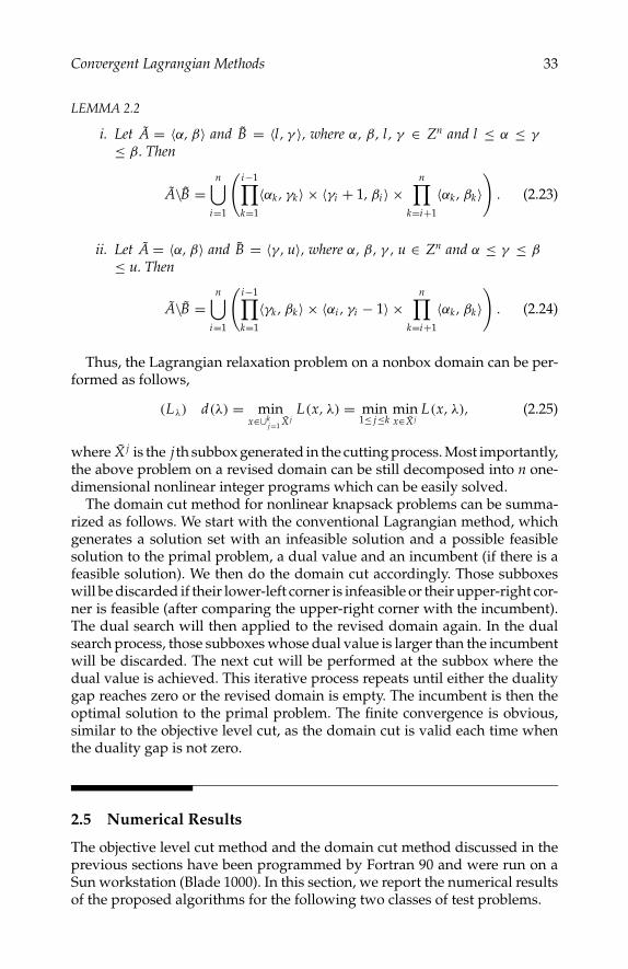
P1: shibu/Vijay

August 12, 2005 9:48 1914 1914˙C002


LEMMA 2.2

i. Let A = 〈α, β〉 and B = 〈l, γ 〉, where α, β, l, γ ∈ Zn and l ≤ α ≤ γ

≤ β. Then

A\B =n⋃

i=1

(i−1∏k=1

〈αk , γk〉 × 〈γi + 1, βi 〉 ×n∏

k=i+1

〈αk , βk〉)

. (2.23)

ii. Let A = 〈α, β〉 and B = 〈γ , u〉, where α, β, γ , u ∈ Zn and α ≤ γ ≤ β

≤ u. Then

A\B =n⋃

i=1

(i−1∏k=1

〈γk , βk〉 × 〈αi , γi − 1〉 ×n∏

k=i+1

〈αk , βk〉)

. (2.24)

Thus, the Lagrangian relaxation problem on a nonbox domain can be per-formed as follows,

(Lλ) d(λ) = minx∈∪k

j=1 X jL(x, λ) = min

1≤ j≤kminx∈X j

L(x, λ), (2.25)

where X j is the j th subbox generated in the cutting process. Most importantly,the above problem on a revised domain can be still decomposed into n one-dimensional nonlinear integer programs which can be easily solved.

The domain cut method for nonlinear knapsack problems can be summa-rized as follows. We start with the conventional Lagrangian method, whichgenerates a solution set with an infeasible solution and a possible feasiblesolution to the primal problem, a dual value and an incumbent (if there is afeasible solution). We then do the domain cut accordingly. Those subboxeswill be discarded if their lower-left corner is infeasible or their upper-right cor-ner is feasible (after comparing the upper-right corner with the incumbent).The dual search will then applied to the revised domain again. In the dualsearch process, those subboxes whose dual value is larger than the incumbentwill be discarded. The next cut will be performed at the subbox where thedual value is achieved. This iterative process repeats until either the dualitygap reaches zero or the revised domain is empty. The incumbent is then theoptimal solution to the primal problem. The finite convergence is obvious,similar to the objective level cut, as the domain cut is valid each time whenthe duality gap is not zero.

2.5 Numerical Results

The objective level cut method and the domain cut method discussed in theprevious sections have been programmed by Fortran 90 and were run on aSun workstation (Blade 1000). In this section, we report the numerical resultsof the proposed algorithms for the following two classes of test problems.

P1: shibu/Vijay

August 12, 2005 9:48 1914 1914˙C002


PROBLEM 2.1Polynomial integer programming (PIP):

min f (x) =n∑

j=1

3∑k=1

c jk xkj

s.t. gi (x) =n∑

j=1

3∑k=1

ai jk xkj ≤ bi , i = 1, . . . , m,

li ≤ xj ≤ u j , xj integer, j = 1, . . . , n.

The coefficients are generated from uniform distributions: all c jk are integersfrom [−10, 10], ai jk ∈ [−10, 10], i = 1, . . . , m, j = 1, . . . , n, k = 1, 2, 3. We alsotake l = (1, . . . , 1)T and u = (5, . . . , 5)T , and bi = gi (l)+ 0.5 × (gi (u)− gi (l)),i = 1, . . . , m. Note that f (x) and gi (x) in problem (PIP) are not necessarilyconvex and the objective function f (x) is integer-valued.

PROBLEM 2.2Polynomial knapsack problems (PKP):

min f (x) =n∑

j=1

[−c j xj + d j (e j − xj )3]

s.t. g(x) = Ax ≤ b,

li ≤ xj ≤ u j , xj integer, j = 1, . . . , n,

where c j > 0, d j > 0, e j ∈ (l j , u j ) for j = 1, . . . , n, and A = (ai j )m×n withai j ≥ 0 for i = 1, . . . , m, j = 1, . . . , n. The coefficients are generated fromuniform distributions: c j ∈ [1, 50], d j ∈ [1, 10], e j ∈ [1, 5] for j = 1, . . . , n,ai j ∈ [1, 50] for i = 1, . . . , m, j = 1, . . . , n. We also take l = (1, . . . , 1)T

and u = (5, . . . , 5)T , and b = 0.7 × Au. We notice that function f j (xj ) =−c j xj + d j (e j − xj )

3 is nonincreasing but not necessarily convex or concaveon [l j , u j ] for j = 1, . . . , n. Therefore, problem (PKP) is a nonlinear knapsackproblem.

Numerical results of the objective level cut method for problem (PIP) arereported in Table 2.1. We can see from Table 2.1 that the proposed algorithmcan solve large-scale multiply constrained separable integer programmingproblems in reasonable computation time.

Table 2.2 summarizes numerical results of the domain cut algorithm forproblem (PKP). It can be seen from Table 2.2 that the domain cut algorithm isefficient for solving large-scale singly-constrained nonlinear knapsack prob-lems in terms of CPU time. Combined with the surrogate constraint technique,the domain cut method can also solve multiply constrained knapsack prob-lems efficiently as shown in Table 2.2.

More computational results of the objective level cut method and the do-main cut method for different types of test problems and their comparisonwith other existing methods in the literature can be found in [14–16]. Oneevident conclusion from numerical experiments is that while most of the

P1: shibu/Vijay

August 12, 2005 9:48 1914 1914˙C002


TABLE 2.1

Numerical Results of Objective LevelCut Method for (PIP)

Average Number Average CPUn m of Iterations Time (s)

50 5 4 0.550 10 12 5.850 15 5 1.950 20 17 24.250 30 15 223.4

TABLE 2.2

Numerical Results of Domain CutMethod for (PKP)

Average Number Average CPUn m of Integer Boxes Time (s)

500 1 30017 30.71000 1 97212 214.52000 1 269877 1382.1

20 5 901 2.840 5 7042 43.860 5 40342 417.030 10 5064 34.630 20 9251 82.830 30 25320 228.6

existing methods suffer from their limitations in nonconvex and multiply-constrained situations, both the objective level cut method and the domaincut method can be applied to general multiply-constrained nonconvex separa-ble nonlinear integer programming problems with promising computationalresults.

2.6 Summary

Two recently developed convergent Lagrangian methods: objective level cutand domain cut methods for separable nonlinear integer programming havebeen discussed in this chapter. Due to the discrete nature of the integerprogramming, the optimal solutions to the Lagrangian relaxation problemcorresponding to the optimal multiplier do not necessarily solve the originalproblem — a duality gap may exist even for linear or convex integer program-ming. The idea of the new cutting methods is based on a key observation thatthe duality gap of an integer program can be eliminated by reshaping theperturbation function. Consequently, the optimal solution can be exposed tothe convex hull of the revised perturbation function, and thus guaranteeing

P1: shibu/Vijay

August 12, 2005 9:48 1914 1914˙C002


the convergence of dual search. These two methods have been tested againsta variety of large-scale separable nonlinear integer programming problemswith up to several thousand variables. Extensive numerical results of thesetwo methods are very promising [14–16].

Acknowledgments

This research was partially supported by the Research Grants Council of HongKong, Grant CUHK4214/01E and the National Natural Science Foundationof China under grants 79970107 and 10271073.

References

1. Bell, D.E. and Shapiro, J.F., A convergent duality theory for integer program-ming. Operations Research 25, 419, 1977.

2. Bretthauer, K.M. and Shetty, B., The nonlinear resource allocation problem. Op-erations Research 43, 670, 1995.

3. Bretthauer, K.M. and Shetty, B., A pegging algorithm for the nonlinear resourceallocation problem. Computers & Operations Research 29, 505, 2002.

4. Cooper, M.W., The use of dynamic programming for the solution of a class ofnonlinear programming problems, Naval Research Logistics Quarterly 27, 89, 980.

5. Fisher, M.L. and Shapiro, J.F., Constructive duality in integer programming.SIAM Journal on Applied Mathematics 27, 31, 1974.

6. Fisher, M.L., The Lagrangian relaxation method for solving integer program-ming problems. Management Science 27, 1, 1981.

7. Geoffrion, A.M., Lagrangian relaxation for integer programming. MathematicalProgramming Study 2, 82, 1974.

8. Gupta, O.K. and Ravindran, A., Branch and bound experiments in convex non-linear integer programming. Management Science 31, 1533, 1985.

9. Hochbaum, D., A nonlinear knapsack problem. Operations Research Letters 17,103, 1995.

10. Ibaraki, T. and Katoh, N., Resource Allocation Problems: Algorithmic Approaches,MIT Press, Cambridge, Massachusetts, 1988.

11. Korner, F., A hybrid method for solving nonlinear knapsack problems. EuropeanJournal of Operational Research 38, 238, 1989.

12. Li, D., Zero duality gap in integer programming: p-norm surrogate constraintmethod. Operations Research Letters 25, 89, 1999.

13. Li, D. and Sun, X.L., Success guarantee of dual search in integer programming:p-th power Lagrangian method. Journal of Global Optimization 18, 235, 2000.

14. Li, D. and Sun, X.L., Nonlinear Integer Programming, Springer, to be published in2005.

15. Li, D., Sun, X.L., Wang, J., and McKinnon, K., A Convergent Lagrangian and do-main cut method for nonlinear knapsack problems, Submitted for publication,2002. Also Technical Report, Serial No: SEEM2002-10, Department of SystemsEngineering and Engineering Management, Chinese University of Hong Kong,November 2002.

P1: shibu/Vijay

August 12, 2005 9:48 1914 1914˙C002


16. Li, D., Wang, J., and Sun, X.L., Exact solution to separable nonlinear integerprogramming: Convergent Lagrangian and objective level cut method, Sub-mitted for publication, 2003. Also Technical Report, Serial No: SEEM2003-08,Department of Systems Engineering and Engineering Management, ChineseUniversity of Hong Kong, May 2003.

17. Li, D. and White, D.J., P-th power Lagrangian method for integer programming.Annals of Operations Research 98, 151, 2000.

18. Marsten, R.E. and Morin, T.L., A hybrid approach to discrete mathematicalprogramming. Mathematical Programming 14, 21, 1978.

19. Shapiro, J.F., A survey of Lagrangian techniques for discrete optimization.Annals of Discrete Mathematics 5, 113, 1979.

20. Sun, X.L. and Li, D., Asymptotic strong duality for bounded integer program-ming: A logarithmic-exponential dual formulation. Mathematics of OperationsResearch 25, 625, 2000.

21. Sun, X.L. and Li, D., New dual formulations in constrained integer program-ming, X. Q. Yang, Ed., Progress in Optimization, Kluwer, 79, 2000.

22. Sun, X.L. and Li, D., Optimality condition and branch and bound algorithmfor constrained redundancy optimization in series systems. Optimization andEngineering 3, 53, 2002.

P1: shibu/Vijay

August 12, 2005 9:48 1914 1914˙C002

P1: shibu/Vijay

August 10, 2005 10:30 1914 1914˙C003

3The Generalized Assignment Problem

Robert M. Nauss

CONTENTS

3.1 Introduction . . . . . . . . . . . . . . . . . . . . . . . . . . . . . . . . 393.2 Model Formulation . . . . . . . . . . . . . . . . . . . . . . . . . . . . 403.3 Previous Work . . . . . . . . . . . . . . . . . . . . . . . . . . . . . . . 403.4 Solution Approach . . . . . . . . . . . . . . . . . . . . . . . . . . . . 42

3.4.1 Methods for Increasing the Lower Bound for (P) . . . . . . . 423.4.2 Methods for Decreasing the Upper Bound for (P) . . . . . . 47

3.5 Branch-and-Bound Algorithm . . . . . . . . . . . . . . . . . . . . . . 483.6 Computational Results . . . . . . . . . . . . . . . . . . . . . . . . . . 503.7 Conclusions . . . . . . . . . . . . . . . . . . . . . . . . . . . . . . . . 53References . . . . . . . . . . . . . . . . . . . . . . . . . . . . . . . . . . . . 54

3.1 Introduction

The generalized assignment problem (GAP) has been investigated in numerousresearch papers over the past 30 years. The problem may be stated as finding aminimum-cost assignment of tasks to agents such that each task is assigned toexactly one agent and such that each agent’s resource capacity is not violated.Applications of the GAP range from jobs assigned to computers in computernetworks (Balachandran [1]) to loading for flexible manufacturing systems(Mazolla et al. [17]) to facility location (Ross and Soland [24]). A review ofapplications and algorithms (both exact and heuristic) appears in Cattrysseand Van Wassenhove [5]. Osman [20] describes various heuristic approachesto the GAP.

The chapter is organized as follows. Section 3.2 describes the mathematicalformulation of the GAP. Section 3.3 surveys earlier work on the GAP. Solutionmethodologies employed in our algorithm are described in Section 3.4.Section 3.5 explains the branch-and-bound algorithm and Section 3.6describes computational results. A concluding section gives ideas for futurework and extensions.

39

P1: shibu/Vijay

August 10, 2005 10:30 1914 1914˙C003


3.2 Model Formulation

The GAP may be formulated as an integer linear programming (ILP) modelwith binary variables. Let n be the number of tasks to be assigned to m agentsand define N = 1, 2, . . . , n and M = 1, 2, . . . , m. Let:

cij = cost of task j being assigned to agent i

rij = amount of resource required for task j by agent i

bi = resource units available to agent i.

The decision variables are defined as:

xij =

1, if task j is assigned to agent i

0, if not.

The 0-1 ILP model is:

(P) minimizem∑

i=1

n∑j=1

cij xij (3.1)

subject to:

n∑j=1

rijxij ≤ bi , ∀i ∈M (3.2)

m∑i=1

xij = 1, ∀ j ∈ N (3.3)

xij = 0 or 1, ∀i ∈ M, j ∈ N. (3.4)

The objective function (3.1) totals the costs of the assignments. Constraint (3.2)enforces resource limitations for each agent, and constraint (3.3) assures thateach task is assigned to exactly one agent. All data elements are allowed tobe real. We note, however, that certain efficiencies follow if the data elementsare assumed to be integral.

3.3 Previous Work

Research on the GAP over the past 30 years provides the integer program-ming student with a smorgasbord of solution approaches devised by numer-ous researchers. This is indeed propitious for the student since he need onlyconcern himself with mastering the various approaches within the context ofa rather simple 0-1 ILP formulation of the GAP.

P1: shibu/Vijay

August 10, 2005 10:30 1914 1914˙C003

The Generalized Assignment Problem 41

The first formal computational work addressing the GAP was by Ross andSoland [23]. Its importance revolves around the fact that the authors used anad hoc approach for solving a tighter (than LP) relaxation which, in effect,was the first published instance of Lagrangian relaxation (LGR) applied to anILP problem. Although the authors did not refer to Lagrangian relaxation perse, its usage is quite clear. Fisher et al. [8] formalized the use of Lagrangianrelaxation and devised a clever dual multiplier adjustment procedure thattightens the initial LGR. This tightening procedure when incorporated in abranch-and-bound algorithm allowed larger, more difficult GAP problems onthe order of 100 0-1 variables to be solved to optimality. Jornsten and Nasberg[13] reformulated the GAP by introducing a set of auxiliary variables andcoupling constraints. Using their approach good, feasible solutions were ableto be generated in a more straightforward fashion. Guignard and Rosenwein[11] extended the work of tightening the LGR by devising a dual-based ap-proach that also incorporated the use of a surrogate constraint. This relaxationtightening allowed problems of up to 500 variables to be solved to optimality.

Thus through the late 1980s the maximum size GAP problems to be solvedto optimality remained at about 500 binary variables. In the early 1990s someresearchers started to look at heuristic approaches due to the perceived diffi-culty in solving large GAP problems to optimality. Cattryese et al. [4] used acolumn generation/set partitioning approach to generate good feasible solu-tions, and coupled this with dual ascent and Lagrangian techniques in orderto reduce the gap between lower (LB) and upper (UB) bounds. Thus theywere able to state that the best feasible solution (UB) was within (U B−L B

L B )% ofoptimality.

Researchers have continued to devise other heuristic approaches for theGAP. Wilson [26] developed a dual-type algorithm and coupled it with aclever search strategy to find good feasible solutions. Chu and Beasley [6]used a genetic algorithm-based heuristic that generates very good feasiblesolutions albeit at increased computation time due to the probabilistic searchfeatures of genetic algorithms in general. Guignard and Zhu [12] utilizedsubgradient optimization to tighten the LGR and simultaneously invoked asimple “variables switch” heuristic to obtain good feasible solutions. Yagiuraet al. [28] devised a tabu search algorithm utilizing an ejection chain approachto govern the neighborhood search for feasible solutions. They also incorpo-rated a subgradient optimization scheme to generate lower bounds so thatsolution quality could be measured. Yagiura et al. [27] extended Yagiura et al.[28] by devising a mechanism to combine two or more reference solutions.

Concurrent with the work on heuristics in the 1990s, various researcherscontinuedtodeviseefficientalgorithmstogenerateprovably optimal solutionsto the GAP. Savelsburgh [25] employed a set partitioning formulation of theGAP similar to that used by Cattrysee et al. [4] (see above). However, he extend-ed their work by employing both column generation and branch-and-boundin order to generate provably optimal solutions to the GAP. He has been able toextend the size of problems solved to 1000 variables. Cattrysee et al. [3] gener-ated lifted cover cuts to improve the standard LP relaxation, devised two new

P1: shibu/Vijay

August 10, 2005 10:30 1914 1914˙C003


heuristics for generating good feasible solutions, and incorporated this in abranch-and-bound algorithm. Park et al. [21] utilized subgradient optimiza-tion in conjunction with a specialized dual ascent algorithm to tighten the La-grangian relaxation and incorporated this approach in a branch-and-boundalgorithm. Finally Nauss [19] has devised a special-purpose branch-and-boundalgorithm that utilizes lifted cover cuts, feasible solution generators, Lagrang-ian relaxation, and subgradient optimization to solve hard GAP problemswith up to 3000 binary variables. A by-product is that good feasible solutionstend to be generated early in the solution process. Thus the algorithm mimicsa heuristic approach when the search process is truncated.

3.4 Solution Approach

Over the past 10 years or so, general purpose ILP solvers have become moreeffective in solving general ILP problems. However certain problem classes,with the GAP being one of them, remain difficult to solve to optimality. Specif-ically “hard” GAP problems with more than 500 binary variables are verydifficult to solve with “off-the-shelf” software such as ILOG’s CPLEX solver(Nauss [19]).

Given this reality, the development of a special-purpose branch-and-boundalgorithm tailored for the GAP’s structure is warranted. In this section we out-line a number of techniques and tools used in a special-purpose algorithm.The algorithm itself will be described in Section 3.5. Consider the GAP de-fined as a minimization problem. A branch-and-bound algorithm may bethought of as a “divide-and-conquer” strategy. In general, strictly decreasingfeasible solution values (upper bounds) are found as the algorithm proceeds.We define the best solution known to date as the incumbent. Concurrentlythe lower bound values of branch-and-bound candidate problems (obtainedfrom valid relaxations) tend to increase as one proceeds deeper in the branch-and-bound tree. Optimality of the incumbent is assured when it can be shownthat the lower bounds of all remaining candidate problems are greater thanor equal to the upper bound. In the next subsection we proceed to describea number of methods for improving valid lower bounds (LB) for (P) as wellas for candidate problems derived from (P) as part of the branch-and-boundprocess. In subsection 3.4.2 we describe methods for generating improvedfeasible solutions (UB).

3.4.1 Methods for Increasing the Lower Bound for (P )

We denote the linear programming relaxation of (P) as (P) where the binaryconstraints (3.4) are replaced by 0 ≤ xij ≤ 1 ∀i ∈ M, j ∈ N. A straightfor-ward way to tighten (P) is to add additional constraints which “cut” awayportions of the feasible region of (P) while leaving the feasible region of(P) intact. Numerous types of cuts may be utilized. However the specialstructure of the GAP in terms of the separable knapsack constraints (3.2)

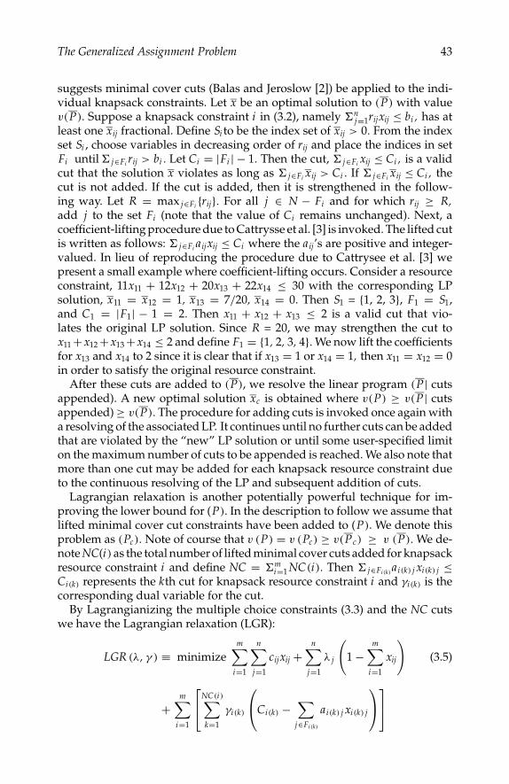
P1: shibu/Vijay

August 10, 2005 10:30 1914 1914˙C003


suggests minimal cover cuts (Balas and Jeroslow [2]) be applied to the indi-vidual knapsack constraints. Let x be an optimal solution to (P) with valuev(P). Suppose a knapsack constraint i in (3.2), namely n

j=1rijxij ≤ bi , has atleast one xij fractional. Define Si to be the index set of xij > 0. From the indexset Si , choose variables in decreasing order of rij and place the indices in setFi until j∈Fi rij > bi . Let Ci = |Fi | − 1. Then the cut, j∈Fi xij ≤ Ci , is a validcut that the solution x violates as long as j∈Fi xij > Ci . If j∈Fi xij ≤ Ci , thecut is not added. If the cut is added, then it is strengthened in the follow-ing way. Let R = max j∈Fi rij. For all j ∈ N − Fi and for which rij ≥ R,add j to the set Fi (note that the value of Ci remains unchanged). Next, acoefficient-lifting procedure due to Cattrysse et al. [3] is invoked. The lifted cutis written as follows: j∈Fi aijxij ≤ Ci where the aij’s are positive and integer-valued. In lieu of reproducing the procedure due to Cattrysee et al. [3] wepresent a small example where coefficient-lifting occurs. Consider a resourceconstraint, 11x11 + 12x12 + 20x13 + 22x14 ≤ 30 with the corresponding LPsolution, x11 = x12 = 1, x13 = 7/20, x14 = 0. Then S1 = 1, 2, 3, F1 = S1,and C1 = |F1| − 1 = 2. Then x11 + x12 + x13 ≤ 2 is a valid cut that vio-lates the original LP solution. Since R = 20, we may strengthen the cut tox11 +x12 +x13 +x14 ≤ 2 and define F1 = 1, 2, 3, 4. We now lift the coefficientsfor x13 and x14 to 2 since it is clear that if x13 = 1 or x14 = 1, then x11 = x12 = 0in order to satisfy the original resource constraint.

After these cuts are added to (P), we resolve the linear program (P| cutsappended). A new optimal solution xc is obtained where v(P) ≥ v(P| cutsappended) ≥ v(P). The procedure for adding cuts is invoked once again witha resolving of the associated LP. It continues until no further cuts can be addedthat are violated by the “new” LP solution or until some user-specified limiton the maximum number of cuts to be appended is reached. We also note thatmore than one cut may be added for each knapsack resource constraint dueto the continuous resolving of the LP and subsequent addition of cuts.

Lagrangian relaxation is another potentially powerful technique for im-proving the lower bound for (P). In the description to follow we assume thatlifted minimal cover cut constraints have been added to (P). We denote thisproblem as (Pc). Note of course that v (P) = v (Pc) ≥ v(Pc) ≥ v (P). We de-note NC(i) as the total number of lifted minimal cover cuts added for knapsackresource constraint i and define NC = m

i=1 NC(i). Then j∈Fi(k)ai(k) j xi(k) j ≤

Ci(k) represents the kth cut for knapsack resource constraint i and γi(k) is thecorresponding dual variable for the cut.

By Lagrangianizing the multiple choice constraints (3.3) and the NC cutswe have the Lagrangian relaxation (LGR):

LGR (λ, γ ) ≡ minimizem∑

i=1

n∑j=1

cijxij +n∑

j=1

λ j

(1 −

m∑i=1

xij

)(3.5)

+m∑

i=1

NC(i)∑

k=1

γi(k)

Ci(k) −

∑j∈Fi(k)

ai(k) j xi(k) j

P1: shibu/Vijay

August 10, 2005 10:30 1914 1914˙C003


subject to:

n∑j=1

rijxij ≤ bi , ∀i ∈ M (3.6)

xij = 0 or 1, ∀i ∈ M, j ∈ N. (3.7)

Note that LGR(λ, γ ) separates into m independent 0-1 knapsack problems.The individual knapsack problems are solved using an algorithm due toNauss [18].

If we utilize the optimal dual multipliers λ and γ from the solution of (Pc)

we are assured that v(P) ≥ v(LGR(λ, γ )) ≥ v(Pc) ≥ v(P). The LGR may betightened further by utilizing subgradient optimization to “adjust” λ and γ

in the following way:

maximizeλ unrestrictedγ ≤ 0

minimize

m∑i=1

n∑j=1

cij xij +n∑

j=1

λ j

(1 −

m∑i=1

xij

)

+m∑

i=1

NC(i)∑

k=1

γi(k)

Ci(k) −

∑j∈Fi(k)

ai(k) j xi(k) j

(3.8)

subject to:

n∑j=1

rij xij ≤ bi , ∀i ∈ M (3.9)

xij = 0 or 1, ∀i ∈ M, j ∈ N. (3.10)

Note that in each subgradient iteration we must solve m 0-1 knapsack prob-lems. Thus we limit the number of iterations to 100 while utilizing a stepsizecalculation described in Guignard and Rosenwein [11].

Once the LGR has been solved we introduce the concept of penalties. Penal-ties are useful in two ways. First in a branch-and-bound algorithm penaltiesmay be used to select a branching variable to separate a candidate problem(CP) under the “divide and conquer” strategy. Variables xij that can be shownto have relatively large values of |v(LGR(CP|xij = 1)) − v(LGR(C P|xij = 0))|are attractive to separate (or branch) on since it is reasonable to assume thatthe objective value for (P) is quite different if xij = 1 as opposed to if xij = 0.

Alternatively if the value is very small, then whether xij equals 0 or 1 wouldnot seem to have much impact on the optimal objective value of (P). A sec-ond use of penalties is to try to fix xij variables to 0 or 1. This is closelyrelated to branch selection since if it can be shown that xij cannot be 0, forexample, the xij may be fixed at 1 and a potential branching is eliminated forCP.

P1: shibu/Vijay

August 10, 2005 10:30 1914 1914˙C003


For penalty calculation we use the Lagrangian relaxation LGR(λ, γ ) where(λ, γ ) are the dual multiplier vectors found via subgradient optimization.Clearly v(LGR(λ, γ )) may be divided into m + 1 components as follows: n∑

j=1

λ j +m∑

i=1

NC(i)∑k=1

γi(k)Ci(k)

+

m∑i=1

n∑

j=1

cij − λ j −NC(i)∑k=1

γi(k)

∑

j∈Fi(k)

ai(k) j

xij

Letting

v(KNAPi ) =n∑

j=1

cij − λ j −

NC(i)∑k=1

γi(k)

∑

j∈Fi(k)

ai(k) j

xij,

we have

v (LGR (λ, γ )) =n∑

j=1

λ j +m∑

i=1

NC(i)∑k=1

γi(k)Ci(k) +m∑

i=1

v(KNAPi ).

Denoting the optimal LP relaxation solution value for (KNAPi )asv(KNAPi ),we have for some i∗,

v (LGR (λ, γ )) ≥n∑

j=1

λ j +m∑

i=1

NC(i)∑k=1

γi(k)Ci(k) +m∑

i=1i =i∗

v(KNAPi ) + v(KNAPi∗)

The right-hand side of the above inequality is a valid relaxation value forv (LGR (λ, γ )). LP penalties for variables in a knapsack problem are easilycalculated using the optimal LP dual multiplier for the resource constraint(Nauss [18]). Note also that the LP penalty for a variable xij is based on the LPrelaxation of a single knapsack constraint while the remainder of the knapsackconstraints are not relaxed. Thus if Z∗ is the incumbent for (P), we may fixxi∗ j to 1 if

n∑j=1

λ j +m∑

i=1

NC(i)∑k=1

γi(k)Ci(k) +

m∑i=1i =i∗

v(KNAPi )

+v(KNAPi∗

)+ PEN(i∗, j |xi∗ j = 0

) ≥ Z∗. (3.11)

Note that PEN(i∗, j |xi∗ j = 0) = −ci∗ j + ζri∗ j where ζ is the optimal dualmultiplier of (KNAPi∗). We note also that a stronger penalty may be cal-culated by finding v(KNAPi∗ |xi∗ j = 0) and substituting it for v(KNAPi∗) +PEN(i∗, j |xi∗ j = 0) in (3.11). This of course requires solving a 0-1 knapsack,which may be prohibitive if every variable were so tested. However, the se-lective use of such enhanced penalties can be effective when a correspondingLP penalty “almost” results in fixing a variable.

P1: shibu/Vijay

August 10, 2005 10:30 1914 1914˙C003


Finally we address two logical feasibility-based tests for fixing xij variablesto 0 or 1. The first test looks at the maximum slack allowed in a knapsackresource constraint i for an optimal solution to (P). As such it utilizes anupper bound on v(P) and thus as the upper bound is reduced the maximumslack also tends to be reduced. This, in effect, reduces the feasible region for (P)

and potentially allows xij variables to be fixed to 0 or 1 in candidate problems.Rewrite the knapsack resource constraints as n

j=1rijxij + ui = bi i ∈ Mwhere ui is defined to be the corresponding nonnegative slack variable. Thenfor each knapsack resource constraint solve the following LP where Z∗ is anupper bound on (P) and v(LGR(λ, γ )) is a lower bound on (P):

gi ≡ maximize ui (3.12)

subject to:

n∑j=1

rij xij + ui = bi , ∀i ∈ M (3.13)

m∑i=1

xij = 1, ∀ j ∈ N (3.14)

v(LGR(λ, γ )) ≤m∑

i=1

n∑j=1

cij xij ≤ Z∗ (3.15)

0 ≤ xij ≤ 1 ∀i ∈ M, j ∈ N (3.16)

ui ≥ 0, ∀ i ∈ M. (3.17)

We may then add the constraints 0 ≤ ui ≤ gi∀i ∈ M to (P) where (3.2) isreplaced by (3.13).

Next we calculate the maximum total slack over all knapsack resourceconstraints by solving:

Z∗u ≡ maximize

m∑i=1

ui

subject to:

(3.13) − (3.16)

0 ≤ ui ≤ gi , ∀i ∈ M.

Suppose that for a particular candidate problem a number of xij variables havebeen set to 1, and that for some resource constraint we have: j |xj =1rj xj >

b −g and j |xj =1rj xj ≤ b. For all i define gcp(i) = minbi − j |xij=1rijxij, gi .

It is easy to see that gcp(i) is a valid bound on ui for a particular candidateproblem. We deduce that Z∗

u − m=1,=i gcp() is also an upper bound on the

maximum slack for knapsack i , and if Z∗u − m

=1∗=i gcp() < gi , then gi maybe reduced to that value for all descendant candidate problems.

P1: shibu/Vijay

August 10, 2005 10:30 1914 1914˙C003


Another method for tightening gi for a candidate problem is to use LPpenalties for each knapsack in the LGR. Define ui to be the value of theslack variable in the ith knapsack LP. If ui = 0 in an optimal LP solution, it isstraightforward to calculate the maximum value that ui could assume suchthat the objective value of the LGR still exceeds Z∗. These calculations arecarried out after all knapsacks in the LGR have been solved, since the testdepends on v(LGR(λ, γ )), v(KNAPi ), and v(KNAPi ). The maximum valuethat ui could take on may then replace gi in the current candidate prob-lem and all its descendants. We note that tightening of the bound on ui isoften more useful in feasibility-based fixing tests than in improving the LB,v(LGR(λ, γ )). This is because the variable to be fixed to 0 is often equal to 0in the LGR. Rather, the benefit of fixing the variable to 0 is important becausethis may eventually lead to other variables being fixed to 1.

The above procedures for reducing the maximum slack in knapsack re-source constraints strengthen the three straightforward logical feasibility testthat we now enumerate.

Consider a conditional feasibility test to fix some xik to 1. Assume xik is tem-porarily set to 0. Then if we can show that for some i, j |xij=1rij < bi − gi and=k and

= j |xij=1ri < bi − gi − j |xij=1rij, then xik may be fixed to 1. This follows since

we must have bi − gi ≤ j rij xij ≤ bi .

Next is a conditional feasibility test where xik is temporarily set to 1. If it canbe shown that no feasible solution exists under this assumption, then xik maybe fixed to 0. For example, if for some i, j =k and

j |xij=1rij + rik > bi , then xikmay be

fixed to 0.Finally, if for some i, j |xij=1rij + rik < bi − gi , and j |xij=1rij + rik

+ min=k and= j |xij=1

ri > bi , then xik may be fixed to 0.

3.4.2 Methods for Decreasing the Upper Bound for (P )

In order to decrease the UB, one must find an improved feasible solution to(P) with objective value less than that of the current incumbent solution, Z∗.At each node of the branch-and-bound tree a Lagrangian relaxation solutionx is obtained from (3.8) to (3.10). In this Lagrangian relaxation the multiplechoice constraints (3.3) have been relaxed and placed in the objective function.Thus they are the only type of constraints that might be violated. For example,a task may have m

i=1 xi ≥ 2 while another task k may have mi=1 xik = 0. Ac-

cordingly, we attempt to modify the LGR solution, x, by attempting to reduceassignments as economically as possible for constraints where m

i=1 xij ≥ 2. Wefind the constraint j∗ where j∗ = arg max(m

i=1 xij). Then all but one xij thatare currently equal to 1 are reset to the value 0 in nonincreasing order of thecost coefficients, ci j∗ . This creates additional slack in the resource constraintsallowing possible assignments to be made for tasks, j , where m

i=1 xij = 0.

For each such constraint j we attempt to set an xij to 1 where the followingtwo conditions must be met. First the knapsack inequality (3.9) must have

P1: shibu/Vijay

August 10, 2005 10:30 1914 1914˙C003


sufficient slack to allow rij to fit and the cost coefficient cij should be as smallas possible. If all multiple choice constraints are now satisfied and the objec-tive function has value less than Z∗, an improved feasible solution has beenfound and the UB is reduced.

Whenever an improved feasible solution has been found, we invoke aneighborhood slide/switch heuristic suggested by Ronen [22] to attempt tofind an even better solution. Ronen attempts to move each task from its cur-rent agent to every other agent. The move is made only if a cost saving isachieved. Next, all pairs of tasks ( j1, j2) currently assigned to distinct agents(i1, i2) where i1 = i2 are tentatively switched so that task j1 is assigned to agenti2 and task j2 is assigned to agent i1. Once again the switch is made only if afeasible cost saving is achieved. Similar tentative switches of one task for twotasks with a different agent as well as two for three task switches are alsoattempted. If an improved solution is generated, the entire neighborhoodslide/switch and multiple switches are attempted again until a completecycle is completed without an improved feasible solution being found.

Finally, complete enumeration is used when relatively few tasks (say, fiveor fewer) remain to be assigned in some candidate problem. Every possiblecombination of assignments of tasks to agents is evaluated. If an improvedfeasible solution is found, the incumbent and the upper bound is updated. Inany case the candidate problem is discarded from further consideration.

3.5 Branch-and-Bound Algorithm

A special purpose branch-and-bound algorithm for the GAP is described us-ing Geoffrion and Marsten’s [9] general framework. We comment on variousfeatures of the algorithm at the end of this section.

Step-1. Set FATHOM = 0, C = .014, and NODE = 0.Step 0. (Solve root node relaxations) Solve the LP relaxation (P). Add vio-

lated lifted minimal cover cuts to (P), namely (Pc). Resolve (Pc) andadd more violated lifted minimal cover cuts. Continue this proce-dure until no more violated cuts are added. Solve the associatedLagrangian relaxation, (LGR) and apply subgradient optimization.Place (P) in the candidate list. Set Z∗ = ZF ≡ (1 + C)∗v(LGR).

Step 1. (Tighten resource slack variable bounds) Solve m + 1 linear pro-grams to find the maximum slack for each resource constraint andthe maximum total slack.

Step 2. (Penalty tests) Attempt to fix variables to 0 or 1 using LP knapsackpenalties. Periodically attempt to fix variables with strong IP knap-sack penalties. Attempt to fix variables to 0 or 1 using feasibility tests.If any variables have been fixed to 0 or 1, resolve the Lagrangian relax-ation and apply subgradient optimization and return to the beginningof step 2. If FATHOM = 1, go to step 3. If FATHOM = 0, go to step 8.

P1: shibu/Vijay

August 10, 2005 10:30 1914 1914˙C003


Step 3. (Candidate problem selection) If the candidate list is empty, stop; anoptimal solution has been found if Z∗ < ZF , or if Z∗ ≥ ZF increase Cto 2*C and go to step 0. If the candidate list is not empty, select aproblem (CP) from the candidate list using a LIFO rule, set NODE =NODE +1, and set FATHOM = 0.

Step 4. (Complete enumeration) If (CP) has more than five tasks not as-signed, go to step 5. Otherwise completely enumerate (CP). If an im-proved feasible solution has been found, update Z∗, set FATHOM = 1and go to step 1. Else go to step 3.

Step 5. (Feasibility-based tests) Perform feasibility-based tests to fix vari-ables 0 to 1.

Step 6. (Solve LGR relaxation) Solve the LGR of (CP). If v(LGR) ≥ Z∗, setFATHOM = 1 and go to step 3. If NODE ≤ 10 or NODE is a multipleof 5, use subgradient optimization to tighten the LGR of (CP). Ifv(LGR) ≥ Z∗ set FATHOM = 1 and go to step 3. If the LGR solu-tion is feasible for (P) update Z∗, set FATHOM = 1 and go to step 1.

Step 7. (Feasible solution generator) Attempt to modify the Lagrangian re-laxation to find an improved feasible solution to (P). If one is found,update Z∗. If Z∗ = v(LGR) set FATHOM = 1 and go to step 1.

Step 8. (Separation) Choose a free variable xij in (CP) and add the candidateproblems (CP | xij = 0) and (CP | xij = 1) to the bottom of the candi-date list. Go to step 3.

The indicator FATHOM is set to 1 whenever a node is fathomed. When anew node is chosen in step 3, FATHOM is reset to 0 and the node counter,NODE is incremented. The value of C is initially set to .014. We use thisparameter in order to artificially set an upper bound ZF at 1.4% larger thanv(LGR). If it is proven that no feasible solution to (P) exists with value lessthan ZF , we double the value of C and restart the algorithm with ZF at avalue 2.8% larger than v(LGR). This technique is used since generally the gapsbetween v(LGR) and optimal value Z∗ are less than 1.4% The initializationof ZF allows us to benefit in two ways. First, Guignard and Rosenwein [11]suggest that a good upper bound target be used for subgradient optimizationin order to reduce “overshooting.” Second, variables may be fixed at 0 or 1using the penalty tests described in earlier sections thus reducing unnecessarybranching or separation. In the next section we comment further on the useof ZF.

In Step 8 the variable to be separated on is determined in the followingway. Recall that a LIFO rule is used to select candidate problems and thus the“1” branch is chosen before “0” branch. Let JFIX1 be the index set of all tasks jthat have an xij fixed to 1 in the current candidate problem. Over all j /∈ JFIX1,place j in the index set JB if m

i=1 xij = 1 (where x is the current LGR solution).The branch variable xij is selected by finding

max PENj∈ JB

andxij=1

(i, j |xi∗ j = 0)

P1: shibu/Vijay

August 10, 2005 10:30 1914 1914˙C003


where PEN (*) is the knapsack LP penalty. In effect we select a variable xij withthe largest penalty for setting xij to 0 such that the corresponding multiplechoice constraint (m

i=1xij = 1) is not violated in the Lagrangian relaxation.


The algorithm was coded in FORTRAN and compiled using Compaq VisualFORTRAN 6.6 (Compaq [7]). XMP (Marsten [16]) was used to solve the linearprograms. A Dell 340 Precision Workstation (2.53 GHz Pentium 4 with 512 MBof PC800 ECC RDRAM) was used for the computational work.

A dataset consisting of 540 random problems was generated according toguidelines outlined in Chu and Beasley [6] and in Laguna et al. [15]. Thedataset consists entirely of “hard” GAP problems of types D and E rangingfrom 750 to 4000 binary variables. Both problem types D and E have ob-jective function coefficients, cij, that are inversely correlated with resourcecoefficients, rij.

We present the computational results in two tables. Table 3.1 gives resultsfor 270 type D problems and Table 3.2 gives results for 270 Type E problems.Each line in the tables gives the average results for ten problems of a particularsize. Six averages for each problem set are reported.

They are:

lpgap(%) − the percentage gap between the LP and best solution foundlgrgap(%) − the percentage gap between the original LGR and the best

solution foundbstlgr(%) − the percentage gap between the LGR that reflects variables

that were fixed to 0 or 1 based on penalty tests calculatedafter every feasible solution found and the best solution foundnode

node − the number of branch-and-bound nodes evaluatedtmbst (sec) − the CPU time in seconds until the best feasible solution was

foundtottime(sec) − the CPU time in seconds to either prove optimality or until

the time limit was reached

A time limit of 1200 CPU seconds was enforced and a suboptimality tol-erance of 0% was used. In both tables the problems are given in order ofincreasing size. Within each set of problems with the same number of vari-ables (but differing number of agents and tasks), the ratio of tasks/agents isdecreasing.

Results for types D and E are dissimilar for problems of size 1250 or greater.In fact only 8 of 240 D type problems with variable sizes of 1250 to 4000 aresolved to optimality. On the other hand 220 of 240 E type problems withvariable sizes of 1250 to 4000 are solved to optimality. A key variable thatseems to explain problem difficulty is bstlgr(%). As can be seen in Table 3.1 and

P1: shibu/Vijay

August 10, 2005 10:30 1914 1914˙C003

The Generalized Assignment Problem 51TA

BLE

3.1

Type

DPr

oble

ms

Pro

ble

ms

Tm

bst

Tott

ime

Req

uir

ing

Age

nts

Task

sV

aria

ble

sTa

sks/

Age

nts

lpga

p(%

)lg

rgap

(%)

bst

lgr(

%)

Nod

es(s

ec)

(sec

)L

arge

rC

515

075

030

.00.

060.

060.

0371

,286

175.

118

5.4

10of

10pr

oven

opti

mal

010

7575

07.

50.

490.

410.

1592

,681

300.

941

4.6

10of

10pr

oven

opti

mal

015

5075

03.

31.

741.

070.

2912

,900

61.5

71.7

10of

10pr

oven

opti

mal

010

125

1250

12.5

0.24

0.21

0.12

214,

629

695.

912

00.4

0of

10pr

oven

opti

mal

010

150

1500

15.0

0.21

0.20

0.13

192,

837

574.

712

00.6

0of

10pr

oven

opti

mal

020

7515

003.

81.

170.

840.

2411

0,33

053

3.8

1049

.92

of10

prov

enop

tim

al0

1017

517

5017

.50.

210.

200.

1517

4,24

473

8.8

1200

.20

of10

prov

enop

tim

al0

2570

1750

2.8

1.78

1.10

0.25

64,6

6753

8.3

786.

06

of10

prov

enop

tim

al0

1020

020

0020

.00.

180.

170.

1416

5,77

070

3.8

1200

.20

of10

prov

enop

tim

al0

2010

020

005.

00.

780.

640.

3098

,685

739.

312

00.2

0of

10pr

oven

opti

mal

025

8020

003.

21.

390.

970.

2987

,615

802.

612

00.4

0of

10pr

oven

opti

mal

010

225

2250

22.5

0.17

0.17

0.14

148,

146

915.

712

00.1

0of

10pr

oven

opti

mal

015

150

2250

10.0

0.34

0.31

0.21

110,

815

683.

012

00.2

0of

10pr

oven

opti

mal

025

9022

503.

61.

160.

850.

3379

,220

753.

812

00.1

0of

10pr

oven

opti

mal

010

250

2500

25.0

0.17

0.17

0.15

135,

247

700.

812

00.2

0of

10pr

oven

opti

mal

020

125

2500

6.3

0.57

0.49

0.28

87,1

5752

1.9

1200

.20

of10

prov

enop

tim

al0

2510

025

004.

00.

970.

760.

3375

,179

783.

912

00.1

0of

10pr

oven

opti

mal

010

275

2750

27.5

0.15

0.14

0.13

133,

488

760.

912

00.1

0of

10pr

oven

opti

mal

025

110

2750

4.4

0.83

0.68

0.34

68,4

4768

9.5

1200

.20

of10

prov

enop

tim

al0

1030

030

0030

.00.

160.

160.

1511

5,69

081

8.3

1200

.10

of10

prov

enop

tim

al0

1520

030

0013

.30.

260.

250.

2089

,744

906.

612

00.1

0of

10pr

oven

opti

mal

020

150

3000

7.5

0.46

0.42

0.28

68,4

7664

2.4

1200

.10

of10

prov

enop

tim

al0

2512

030

004.

80.

710.

590.

3262

,377

710.

412

00.1

0of

10pr

oven

opti

mal

030

100

3000

3.3

1.26

0.94

0.42

56,6

3884

5.6

1200

.10

of10

prov

enop

tim

al0

1040

040

0040

.00.

180.

180.

1789

,290

691.

412

00.2

0of

10pr

oven

opti

mal

020

200

4000

10.0

0.37

0.35

0.28

57,5

8171

7.9

1200

.20

of10

prov

enop

tim

al0

2516

040

006.

40.

540.

490.

3348

,692

774.

412

00.2

0of

10pr

oven

opti

mal

0O

vera

llA

vera

ges

0.61

0.47

0.23

100,

438

658.

610

70.8

1.4

of10

prov

enop

tim

al0

38of

270

prov

enop

tim

al

P1: shibu/Vijay

August 10, 2005 10:30 1914 1914˙C003

52 Integer Programming: Theory and PracticeTA

BLE

3.2

Type

EPr

oble

ms

Pro

ble

ms

Tm

bst

Tott

ime

Req

uir

ing

Age

nts

Task

sV

aria

ble

sTa

sks/

Age

nts

lpga

p(%

)lg

rgap

(%)

bst

lgr(

%)

Nod

es(s

ecs)

(sec

s)L

arge

rC

515

075

030

.00.

070.

050.

031,

285

3.0

3.7

10of

10pr

oven

opti

mal

010

7575

07.

50.

500.

100.

091,

434

4.8

5.8

10of

10pr

oven

opti

mal

015

5075

03.

32.

850.

340.

331,

113

5.2

7.2

10of

10pr

oven

opti

mal

810

125

1250

12.5

0.14

0.05

0.03

4,26

317

.719

.610

of10

prov

enop

tim

al0

1015

015

0015

.00.

110.

040.

026,

028

27.3

30.0

10of

10pr

oven

opti

mal

020

7515

003.

81.

790.

190.

184,

789

29.5

42.0

10of

10pr

oven

opti

mal

010

175

1750

17.5

0.08

0.04

0.02

8,93

330

.542

.110

of10

prov

enop

tim

al0

2570

1750

2.8

3.65

0.24

0.22

3,57

537

.248

.010

of10

prov

enop

tim

al10

1020

020

0020

.00.

050.

030.

014,

898

27.0

29.9

10of

10pr

oven

opti

mal

020

100

2000

5.0

0.85

0.09

0.08

19,6

5318

1.7

196.

810

of10

prov

enop

tim

al0

2580

2000

3.2

2.50

0.21

0.20

6,42

545

.378

.610

of10

prov

enop

tim

al5

1022

522

5022

.50.

050.

030.

016,

054

30.1

36.1

10of

10pr

oven

opti

mal

015

150

2250

10.0

0.17

0.05

0.03

14,3

4310

2.8

117.

610

of10

prov

enop

tim

al0

2590

2250

3.6

1.91

0.21

0.20

17,6

4617

1.7

229.

510

of10

prov

enop

tim

al0

1025

025

0025

.00.

030.

020.

018,

246

49.0

52.6

10of

10pr

oven

opti

mal

020

125

2500

6.3

0.42

0.06

0.05

17,1

7314

6.6

197.

010

of10

prov

enop

tim

al0

2510

025

004.

01.

360.

170.

1631

,460

250.

842

4.9

8of

10pr

oven

opti

mal

010

275

2750

27.5

0.03

0.02

0.01

11,8

6179

.187

.110

of10

prov

enop

tim

al0

2511

027

504.

41.

040.

120.

1123

,077

198.

534

1.2

8of

10pr

oven

opti

mal

010

300

3000

30.0

0.03

0.02

0.01

27,3

8312

5.4

182.

810

of10

prov

enop

tim

al0

1520

030

0013

.30.

090.

030.

0219

,581

146.

320

5.2

10of

10pr

oven

opti

mal

020

150

3000

7.5

0.29

0.05

0.03

37,9

4742

4.9

537.

09

of10

prov

enop

tim

al0

2512

030

004.

80.

810.

080.

0722

,587

269.

639

2.8

8of

10pr

oven

opti

mal

030

100

3000

3.3

2.21

0.20

0.19

27,2

3831

0.5

496.

58

of10

prov

enop

tim

al3

1040

040

0040

.00.

030.

020.

0187

,607

650.

672

4.3

7of

10pr

oven

opti

mal

020

200

4000

10.0

0.15

0.04

0.03

54,6

1059

4.5

813.

36

of10

prov

enop

tim

al0

2516

040

006.

40.

460.

130.

1237

,090

509.

171

4.1

6of

10pr

oven

opti

mal

0O

vera

llA

vera

ges

0.80

0.10

0.08

18,7

5216

5.5

224.

39.

3of

10pr

oven

opti

mal

2625

0of

270

prov

enop

tim

al

P1: shibu/Vijay

August 10, 2005 10:30 1914 1914˙C003


Table 3.2 the bstlgr(%) in Table 3.1 is generally larger than the corresponding(same number of agents and tasks) value of bstlgr(%) in Table 3.2. In fact overall 270 type E problems the average bstlgr(%) is .08 while the correspondingvalue is .23 over all 270 type D problems. Also note that in numerous instancesin Table 3.1 and Table 3.2 there are average lpgap(%) values in excess of 1.Somewhat perplexing is the fact that the overall average lpgap(%) for type Dis .61 while it is .80 for type E. However the overall average lgrgap(%) for typeD is .47 while only .10 for type E. Thus we have the interesting behavior of typeD problems having tighter LP relaxations, but looser LGR relaxations whencompared to type E problems. We also note that 26 of 270 Type E problemsrequired that the value of C be increased from .014 to .028. Put another way thevalue of ZF was set too low in these cases. The CPU time and node averagesinclude the time and nodes evaluated when C was .014 for those problems.

We also note that as the tasks/agents ratio becomes smaller (for a fixed num-ber of variables), it is almost uniformly true that the lpgap(%), lgrgap(%), andbstlgr(%) grow larger. The only exception is in Table 3.1 when comparing thebstlgr(%) for 2000 variable problems. This behavior appears to make sensesince as the expected number of tasks per agent decreases it is more likelythat slack occurs in the resource constraints. This implies that available re-sources are not being efficiently utilized and hence the lpgap(%), lgrgap(%),and bstlgr(%) will tend to grow larger.

Finally we note that Yagiura et al. [27] analyzed the “distance” betweengood feasible solutions for individual problems. Interestingly they found thataverage distances are larger for Type D problems. This suggests two things.First, Type D problems appear to have good feasible solutions more highly dis-persed over the feasible region. Second, this dispersal suggests that a “depthfirst” search (which we use) may not be as effective as a “breadth first” searchfor Type D problems. This appears to be confirmed by the excellent resultsthat were generated for Type E problems where good feasible solutions tendto be “closer together.”

3.7 Conclusions

While our results are favorable for Type E problems up to 4000 variables,Type D problems of 1250 or more variables still remain difficult for our algo-rithm. However, it should be pointed out that the largest average bestlgr(%)gap for any Type D problem set is .42% with an overall average for all 270problems of .23%. Thus excellent feasible solutions are generated with theshortcomings being the difficulty in further tightening of the lower boundsand in the use of a LIFO approach for selection of candidate problems(cf. Section 3.6). Further work on Type D problems might include a “breadthfirst” approach for the search process as well as additional work on tighteningthe relaxed feasible region of candidate problems. For example the incorpora-tion of additional cuts as developed by Gottlieb and Rao [10] might result in

P1: shibu/Vijay

August 10, 2005 10:30 1914 1914˙C003


a Lagrangian relaxation that is easier (and faster) to solve in the subgradientoptimization phase. In line with this it should be noted that since 30 to 60%of CPU time is devoted to solving the 0-1 knapsack problems, an alternateknapsack code (Kellerer et al. [14]) might be incorporated. Such an imple-mentation might require that all data (cij and rij) be integer valued. Secondly,the use of a state-of-the-art LP solver such as CPLEX would result in reducedcomputational times. Finally with the advent of parallel processing it wouldbe instructive to “marry” the branch-and-bound code with a heuristic such asYagiura et al. [27]. In such a marriage multiple processors might be allocatedfor separate copies of the heuristic (where different feasible region neighbor-hoods are examined). Then when an improved feasible solution is found itis stored in shared memory to be used by multiple processors that are run-ning the branch-and-bound algorithm. (Of course improved feasible solutionsgenerated by the branch-and-bound algorithm would also be stored in thisshared memory.) Alternatively the neighborhood search heuristics might be“called” to explore various feasible region neighborhoods on different pro-cessors as the branch-and-bound algorithm generates sufficiently differentcandidate problems.

References

1. Balachandran, V., An integer generalized transportation model for optimal jobassignment in computer networks, Working Paper 34-72-3, Graduate School ofIndustrial Administration, Carnegie Mellon University, Pittsburgh, 1972.

2. Balas, E. and Jeroslow, R., Canonical cuts in the unit hypercube, SIAM J. Appl.Math., 23, 61, 1972.

3. Cattrysse, D., Degraeve Z., and Tistaert, J., Solving the generalized assignmentproblem using polyhedral results, European J. Operational Research, 108, 618, 1998.

4. Cattrysse, D., Salomon, M., and Van Wassenhove, L., A set partitioning heuristicfor the generalized assignment problem, European J. Operational Research, 72, 167,1994.

5. Cattrysse, D. and Van Wassenhove, L., A survey of algorithms for the general-ized assignment problem, European J. Operational Research, 60, 260, 1992.

6. Chu, P.C. and Beasley, J.B., A genetic algorithm for the generalized assignmentproblem, Computers and Operations Research, 24, 17, 1997.

7. COMPAQ Fortran Language Reference Manual, Compaq Computer Corporation,Houston, 1999.

8. Fisher, M. and Jaikumar, R., A generalized assignment heuristic for vehicle rout-ing, Networks, 11, 109, 1981.

9. Geoffrion, A.M. and Marsten, R.E., Integer programming algorithms: a frame-work and state-of-the-art survey, Management Science, 18, 465, 1972.

10. Gottlieb, E. and Rao, M., The generalized assignment problem: valid inequalitiesand facets, Mathematical Programming, 46, 31, 1990.

11. Guignard, M. and Rosenwein, M., An improved dual based algorithm for thegeneralized assignment problem, Operations Research, 37, 658, 1989.

P1: shibu/Vijay

August 10, 2005 10:30 1914 1914˙C003


12. Guignard, M. and Zhu, S., A Two Phase Dual Algorithm for Solving LagrangianDuals in Mixed Integer Programming, working paper, The Wharton School, Uni-versity of Pennsylvania, Philadelphia, 1996.

13. Jornsten, K. and Nasberg, M., A new Lagrangian relaxation approach to thegeneralized assignment problem, European Journal of Operational Research, 27,313, 1986.

14. Kellerer, H., Pferschy, U., and Pisinger, D., Knapsack Problems, Springer, 2004.15. Laguna, M., Kelly, J., Gonzalez-Velarde, J., and Glover, F., Tabu search for the

multilevel generalized assignment problem, European J. Operational Research, 82,176, 1995.

16. Marsten, R., The design of the XMP linear programming library, technical re-port, Department of Management Information Systems, University of Arizona,Tucson, 80-2, 1980.

17. Mazzola, J., Neebe, A., and Dunn, C., Production planning of a flexible manu-facturing system in a material requirements planning environment, InternationalJournal of Flexible Manufacturing Systems, Vol. 1 of 2, 115, 1989.

18. Nauss, R.M., An efficient algorithm for the 0-1 knapsack problem, ManagementScience, 23, 27, 1976.

19. Nauss, R.M., Solving the generalized assignment problem: an optimizing andheuristic approach, INFORMS Journal on Computing, 15, 249, 2003.

20. Osman, I.H., Heuristics for the generalized assignment problem, OR Spektrum,17, 211, 1995.

21. Park, J.S., Lim, B.H., and Lee, Y., A Lagrangian dual-based branch-and-boundalgorithm for the generalized multi-assignment problem, Management Science,44, S271, 1998.

22. Ronen, D., Allocation of trips to trucks operating from a single terminal, Com-puters and Operations Research, 19, 129, 1992.

23. Ross, G.T. and Soland, R.M., A branch and bound algorithm for the generalizedassignment problem, Mathematical Programming, 8, 91, 1975.

24. Ross, G.T. and Soland, R.M., Modeling facility location problems as generalizedassignment problems, Management Science, 24, 345, 1977.

25. Savelsbergh, M., A branch-and-price algorithm for the generalized assignmentproblem, Operations Research, 45, 831, 1997.

26. Wilson, J.M., A simple dual algorithm for the generalized assignment problem,Journal of Heuristics, 2, 303, 1997.

27. Yagiura, M., Ibaraki, T. and Glover, F., A path relinking approach with ejectionchains for the generalized assignment problem, European Journal of OperationalResearch, in press, 2005.

28. Yagiura, M., Ibaraki, T., and Glover, F., An ejection chain approach for thegeneralized assignment problem, INFORMS Journal on Computing, 16, No. 2,2004.

P1: shibu/Vijay

August 10, 2005 10:30 1914 1914˙C003

P1: shibuAugust 23, 2005 10:18 1914 1914˙CH04

4Decomposition in Integer LinearProgramming

Ted K. Ralphs and Matthew V. Galati

CONTENTS

4.1 Introduction . . . . . . . . . . . . . . . . . . . . . . . . . . . . . . . . 574.2 Definitions and Notation . . . . . . . . . . . . . . . . . . . . . . . . . 594.3 The Principle of Decomposition . . . . . . . . . . . . . . . . . . . . . 60

4.3.1 Cutting Plane Method . . . . . . . . . . . . . . . . . . . . . . 644.3.2 Dantzig-Wolfe Method . . . . . . . . . . . . . . . . . . . . . . 684.3.3 Lagrangian Method . . . . . . . . . . . . . . . . . . . . . . . 76

4.4 Integrated Decomposition Methods . . . . . . . . . . . . . . . . . . 784.4.1 Price and Cut . . . . . . . . . . . . . . . . . . . . . . . . . . . 794.4.2 Relax and Cut . . . . . . . . . . . . . . . . . . . . . . . . . . . 90

4.5 Solving the Cutting Subproblem . . . . . . . . . . . . . . . . . . . . 924.5.1 The Template Paradigm . . . . . . . . . . . . . . . . . . . . . 934.5.2 Separating Solutions with Known Structure . . . . . . . . . . 934.5.3 Decompose and Cut . . . . . . . . . . . . . . . . . . . . . . . 94

4.6 Solving the Master Problem . . . . . . . . . . . . . . . . . . . . . . . 964.7 Software . . . . . . . . . . . . . . . . . . . . . . . . . . . . . . . . . . 974.8 Applications . . . . . . . . . . . . . . . . . . . . . . . . . . . . . . . . 98

4.8.1 Vehicle Routing Problem . . . . . . . . . . . . . . . . . . . . . 994.8.2 Three-Index Assignment Problem . . . . . . . . . . . . . . 1034.8.3 Steiner Tree Problem . . . . . . . . . . . . . . . . . . . . . . 105

4.9 Conclusions and Future Work . . . . . . . . . . . . . . . . . . . . . 107References . . . . . . . . . . . . . . . . . . . . . . . . . . . . . . . . . . . 107

4.1 Introduction

In this chapter, we discuss the principle of decomposition as it applies to thecomputation of bounds on the value of an optimal solution to an integer linearprogram (ILP). Most bounding procedures for ILP are based on the generationof a polyhedron that approximates P , the convex hull of feasible solutions.

57

P1: shibuAugust 23, 2005 10:18 1914 1914˙CH04


Solving an optimization problem over such a polyhedral approximation, pro-vided it fully containsP , produces a bound that can be used to drive a branch-and-bound algorithm. The effectiveness of the bounding procedure dependslargely on how well P can be approximated. The most straightforward ap-proximation is the continuous approximation, consisting simply of the linearconstraints present in the original ILP formulation. The bound resulting fromthis approximation is frequently too weak to be effective, however. In suchcases, it can be improved by dynamically generating additional polyhedralinformation that can be used to augment the approximation.

Traditional dynamic procedures for augmenting the continuous approx-imation can be grouped roughly into two categories. Cutting plane methodsimprove the approximation by dynamically generating half-spaces contain-ing P , i.e., valid inequalities, to form a second polyhedron, and then intersectthis second polyhedron with the continuous approximation to yield a finalapproximating polyhedron. With this approach, the valid inequalities are gen-erated by solution of an associated separation problem. Generally, the additionof each valid inequality reduces the hypervolume of the approximating poly-hedron, resulting in a potentially improved bound. Because they dynamicallygenerate part of the description of the final approximating polyhedron as theintersection of half-spaces (an outer representation), we refer to cutting planemethods as outer approximation methods.

Traditional decomposition methods, on the other hand, improve the ap-proximation by dynamically generating the extreme points of a polyhedroncontaining P , which is again intersected with the continuous approximation,as in the cutting plane method, to yield a final approximating polyhedron.In this case, each successive extreme point is generated by solution of anassociated optimization problem and at each step, the hypervolume of the ap-proximating polyhedron is increased. Because decomposition methods dy-namically generate part of the description of the approximating polyhedronas the convex hull of a finite set (an inner representation), we refer to thesemethods as inner approximation methods.

Both inner and outer methods work roughly by alternating between a pro-cedure for computing solution and bound information (the master problem)and a procedure for augmenting the current approximation (the subproblem).The two approaches, however, differ in important ways. Outer methods re-quire that the master problem produce “primal” solution information, whichthen becomes the input to the subproblem, a separation problem. Inner methodsrequire “dual” solution information, which is then used as the input to thesubproblem, an optimization problem. In this sense, the two approaches can beseen as “dual” to one another. A more important difference, however, is thatthe valid inequalities generated by an inner method can be valid with respectto any polyhedron containing P (see Section 4.5), whereas the extreme pointsgenerated by an inner method must ostensibly be from a single polyhedron.Procedures for generating new valid inequalities can also take advantageof knowledge of previously generated valid inequalities to further improvethe approximation, whereas with inner methods, such “backward-looking”

P1: shibuAugust 23, 2005 10:18 1914 1914˙CH04

Decomposition in Integer Linear Programming 59

procedures do not appear to be possible. Finally, the separation proceduresused in the cutting plane method can be heuristic in nature as long as it can beproven that the resulting half-spaces do actually contain P . Although heuris-tic methods can be employed in solving the optimization problem requiredof an inner method, valid bounds are only obtained when using exact opti-mization. On the whole, outer methods have proven to be more flexible andpowerful and this is reflected in their position as the approach of choice forsolving most ILPs.

As we will show, however, inner methods do still have an important role toplay. Although inner and outer methods have traditionally been consideredseparate and distinct, it is possible, in principle, to integrate them in a straight-forward way. By doing so, we obtain bounds at least as good as those yieldedby either approach alone. In such an integrated method, one alternates be-tween a master problem that produces both primal and dual information, andeither one of two subproblems, one an optimization problem and the other aseparation problem. This may result in significant synergy between the sub-problems, as information generated by solving the optimization subproblemcan be used to generate cutting planes and vice versa.

The remainder of the chapter is organized as follows. In Section 4.2, we in-troduce definitions and notation. In Section 4.3, we describe the principle ofdecomposition and its application to integer linear programming in a tra-ditional setting. In Section 4.4, we extend the traditional framework to showhow the cutting plane method can be integrated with either the Dantzig-Wolfemethod or the Lagrangian method to yield improved bounds. In Section 4.5,we discuss solution of the separation subproblem and introduce an extensionof the well-known template paradigm, called structured separation, inspired bythe fact that separation of structured solutions is frequently easier than sep-aration of arbitrary real vectors. We also introduce a decomposition-basedseparation algorithm called decompose and cut that exploits structured sepa-ration. In Section 4.6, we discuss some of the algorithms that can be usedto solve the master problem. In Section 4.7, we describe a software frame-work for implementing the algorithms presented in the paper. Finally, inSection 4.8, we present applications that illustrate the principles discussedherein.

4.2 Definitions and Notation

For ease of exposition, we consider only pure integer linear programs withbounded, nonempty feasible regions, although the methods presented hereincan be extended to more general settings. For the remainder of the chapter,we consider an ILP whose feasible set is the integer vectors contained in thepolyhedron Q = x ∈ Rn | Ax ≥ b, where A ∈ Qm×n is the constraint matrixand b ∈ Qm is the vector of requirements. Let F = Q ∩ Zn be the feasible set

P1: shibuAugust 23, 2005 10:18 1914 1914˙CH04


and let P be the convex hull of F . The canonical optimization problem for P isthat of determining

zIP = minx∈Zn

cx | Ax ≥ b = minx∈F

cx = minx∈P

cx (4.1)

for a given cost vector c ∈ Qn, where zIP = ∞ if F is empty. We refer to

such an ILP by the notation ILP(P , c). In what follows, we also consider theequivalent decision version of this problem, which is to determine, for a givenupper bound U, whether there is a member ofP with objective function valuestrictly better than U. We denote by OPT(P , c, U) a subroutine for solving thisdecision problem. The subroutine is assumed to return either the empty set, ora set of one or more (depending on the situation) members of P with objectivevalue better than U.

A related problem is the separation problem for P , which is typically alreadystated as a decision problem. Given x ∈ Rn, the problem of separating x fromP is that of deciding whether x ∈ P and if not, determining a ∈ R

n andβ ∈ R such that ay ≥ β ∀y ∈ P but ax < β. A pair (a, β) ∈ Rn+1 such thatay ≥ β ∀y ∈ P is a valid inequality for P and is said to be violated by x ∈ Rn

if ax < β. We denote by SEP(P , x) a subroutine that separates an arbitraryvector x ∈ Rn from polyhedron P , returning either the empty set or a set ofone or more violated valid inequalities. Note that the optimization form ofthe separation problem is that of finding the most violated inequality and isequivalent to the decision form stated here.

A closely related problem is the facet identification problem, which restrictsthe generated inequalities to only those that are facet-defining for P . In [32],it was shown that the facet identification problem for P is polynomiallyequivalent to the optimization problem for P (in the worst case sense).However, a theme that arises in what follows is that the complexity of opti-mization and separation can vary significantly if either the input or the outputmust have known structure. If the solution to an optimization problem is re-quired to be integer, the problem generally becomes much harder to solve.On the other hand, if the input vector to a separation problem is an integralvector, then the separation problem frequently becomes much easier to solvein the worst case. From the dual point of view, if the input cost vector of anoptimization problem has known structure, such as being integral, this maymake the problem easier. Requiring the output of the separation problem tohave known structure is known as the template paradigm and may also makethe separation problem easier, but such a requirement is essentially equivalentto enlarging P . These concepts are discussed in more detail in Section 4.5.

4.3 The Principle of Decomposition

We now formalize some of the notions described in the introduction. Imple-menting a branch-and-bound algorithm for solving an ILP requires a pro-cedure that will generate a lower bound as close as possible to the optimal

P1: shibuAugust 23, 2005 10:18 1914 1914˙CH04


value zIP. The most commonly used method of bounding is to solve the linearprogramming (LP) relaxation obtained by removing the integrality require-ment from the ILP formulation. The LP Bound is given by

zLP = minx∈Rn

cx | Ax ≥ b = minx∈Q

cx, (4.2)

and is obtained by solving a linear program with the original objective func-tion c over the polyhedron Q. It is clear that zLP ≤ zIP since P ⊆ Q. This LPrelaxation is usually much easier to solve than the original ILP, but zLP may bearbitrarily far away from zIP in general, so we need to consider more effectiveprocedures.

In most cases, the description ofQ is small enough that it can be representedexplicitly and the bound computed using a standard linear programming al-gorithm. To improve the LP bound, decomposition methods construct a sec-ond approximating polyhedron that can be intersected withQ to form a betterapproximation. Unlike Q, this second polyhedron usually has a descriptionof exponential size, and we must generate portions of its description dynam-ically. Such a dynamic procedure is the basis for both cutting plane methods,which generate an outer approximation, and for traditional decompositionmethods, such as the Dantzig-Wolfe method [19] and the Lagrangian method[22, 14], which generate inner approximations.

For the remainder of this section, we consider the relaxation of (4.1)defined by

minx∈Zn

cx | A′x ≥ b ′ = minx∈F ′

cx = minx∈P ′

cx, (4.3)

where F ⊂ F ′ = x ∈ Zn | A′x ≥ b ′ for some A′ ∈ Qm′×n, b ′ ∈ Qm′and P ′

is the convex hull of F ′. Along with P ′ is associated a set of side constraints[A′′, b ′′] ∈ Q

m′′×(n+1) such that Q = x ∈ Rn | A′x ≥ b ′, A′′x ≥ b ′′. We

denote by Q′ the polyhedron described by the inequalities [A′, b ′] and by Q′′

the polyhedron described by the inequalities [A′′, b ′′]. Thus, Q = Q′ ∩ Q′′

and F = x ∈ Zn | x ∈ P ′ ∩ Q′′. For the decomposition to be effective,

we must have that P ′ ∩ Q′′ ⊂ Q, so that the bound obtained by optimizingover P ′ ∩Q′′ is at least as good as the LP bound and strictly better for someobjective functions. The description of Q′′ must also be “small” so that wecan construct it explicitly. Finally, we assume that there exists an effectivealgorithm for optimizing over P ′ and thereby, for separating arbitrary realvectors from P ′. We are deliberately using the term effective here to denotean algorithm that has an acceptable average-case running time, since this ismore relevant than worst-case behavior in our computational framework.

Traditional decomposition methods can all be viewed as techniques foriteratively computing the bound

zD = minx∈P ′

cx | A′′x ≥ b ′′ = minx∈F ′∩Q′′

cx = minx∈P ′∩Q′′

cx. (4.4)

In Section 4.3.1 to Section 4.3.3 below, we review the cutting plane method, theDantzig-Wolfe method, and the Lagrangian method, all classical approaches

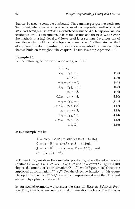
P1: shibuAugust 23, 2005 10:18 1914 1914˙CH04


that can be used to compute this bound. The common perspective motivatesSection 4.4, where we consider a new class of decomposition methods calledintegrated decomposition methods, in which both inner and outer approximationtechniques are used in tandem. In both this section and the next, we describethe methods at a high level and leave until later sections the discussion ofhow the master problem and subproblems are solved. To illustrate the effectof applying the decomposition principle, we now introduce two examplesthat we build on throughout the chapter. The first is a simple generic ILP.

Example 4.1Let the following be the formulation of a given ILP:

min x1,

7x1 − x2 ≥ 13, (4.5)x2 ≥ 1, (4.6)

−x1 + x2 ≥ −3, (4.7)−4x1 − x2 ≥ −27, (4.8)

−x2 ≥ −5, (4.9)0.2x1 − x2 ≥ −4, (4.10)−x1 − x2 ≥ −8, (4.11)

−0.4x1 + x2 ≥ 0.3, (4.12)x1 + x2 ≥ 4.5, (4.13)

3x1 + x2 ≥ 9.5, (4.14)0.25x1 − x2 ≥ −3, (4.15)

x ∈ Z2. (4.16)

In this example, we let

P = convx ∈ R2 | x satisfies (4.5) − (4.16),Q′ = x ∈ R2 | x satisfies (4.5) − (4.10),Q′′ = x ∈ R2 | x satisfies (4.11) − (4.15), andP ′ = conv(Q′ ∩ Z2).

In Figure 4.1(a), we show the associated polyhedra, where the set of feasiblesolutions F = Q′ ∩Q′′ ∩ Z2 = P ′ ∩Q′′ ∩ Z2 and P = conv(F). Figure 4.1(b)depicts the continuous approximationQ′ ∩Q′′, while Figure 4.1(c) shows theimproved approximation P ′ ∩ Q′′. For the objective function in this exam-ple, optimization over P ′ ∩ Q′′ leads to an improvement over the LP boundobtained by optimization over Q.

In our second example, we consider the classical Traveling Salesman Prob-lem (TSP), a well-known combinatorial optimization problem. The TSP is in

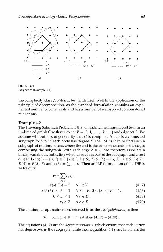
P1: shibuAugust 23, 2005 10:18 1914 1914˙CH04


(2,1)(2,1)),1(2

′′∩ Q′PP

′′∩ Q′QP

′′Q

′Q

′PP

(c)(b)(a)

FIGURE 4.1Polyhedra (Example 4.1).

the complexity class N P-hard, but lends itself well to the application of theprinciple of decomposition, as the standard formulation contains an expo-nential number of constraints and has a number of well-solved combinatorialrelaxations.

Example 4.2The Traveling Salesman Problem is that of finding a minimum cost tour in anundirected graph G with vertex set V = 0, 1, . . . , |V|−1 and edge set E . Weassume without loss of generality that G is complete. A tour is a connectedsubgraph for which each node has degree 2. The TSP is then to find such asubgraph of minimum cost, where the cost is the sum of the costs of the edgescomprising the subgraph. With each edge e ∈ E , we therefore associate abinary variable xe , indicating whether edge e is part of the subgraph, and a costce ∈ R. Let δ(S) = i, j ∈ E | i ∈ S, j /∈ S, E(S : T) = i, j | i ∈ S, j ∈ T,E(S) = E(S : S) and x(F ) = ∑

e∈F xe . Then an ILP formulation of the TSP isas follows:

min∑e∈E

ce xe ,

x(δ(i)) = 2 ∀ i ∈ V, (4.17)x(E(S)) ≤ |S| − 1 ∀ S ⊂ V, 3 ≤ |S| ≤ |V| − 1, (4.18)

0 ≤ xe ≤ 1 ∀ e ∈ E, (4.19)xe ∈ Z ∀ e ∈ E . (4.20)

The continuous approximation, referred to as the TSP polyhedron, is then

P = convx ∈ RE | x satisfies (4.17) − (4.20).The equations (4.17) are the degree constraints, which ensure that each vertexhas degree two in the subgraph, while the inequalities (4.18) are known as the

P1: shibuAugust 23, 2005 10:18 1914 1914˙CH04


subtour elimination constraints (SECs) and enforce connectivity. Since there arean exponential number of SECs, it is impossible to explicitly construct the LPrelaxation of TSP for large graphs. Following the pioneering work of Held andKarp [35], however, we can apply the principle of decomposition by employ-ing the well-known Minimum 1-Tree Problem, a combinatorial relaxation of TSP.

A 1-tree is a tree spanning V \ 0 plus two edges incident to vertex 0. A1-tree is hence a subgraph containing exactly one cycle through vertex 0. TheMinimum 1-Tree Problem is to find a 1-tree of minimum cost and can thus beformulated as follows:

min∑e∈E

ce xe ,

x(δ(0)) = 2, (4.21)x(E(V \ 0)) = |V| − 2, (4.22)

x(E(S)) ≤ |S| − 1 ∀ S ⊂ V \ 0, 3 ≤ |S| ≤ |V| − 1, (4.23)xe ∈ 0, 1 ∀ e ∈ E . (4.24)

A minimum cost 1-tree can be obtained easily as the union of a minimumcost spanning tree of V \ 0 plus two cheapest edges incident to vertex 0.For this example, we thus let P ′ = conv(x ∈ RE | x satisfies (4.21) − (4.24))be the 1-Tree Polyhedron, while the degree and bound constraints comprisethe polyhedron Q′′ = x ∈ RE | x satisfies (4.17) and (4.19) and Q′ = x ∈R

E | x satisfies (4.18). Note that the bound constraints appear in the descrip-tions of both polyhedra for computational convenience. The set of feasiblesolutions to TSP is then F = P ′ ∩Q′′ ∩ ZE .

4.3.1 Cutting Plane Method

Using the cutting plane method, the bound zD can be obtained by dynamicallygenerating portions of an outer description of P ′. Let [D, d] denote the set offacet-defining inequalities of P ′, so that

P ′ = x ∈ Rn | Dx ≥ d. (4.25)

Then the cutting plane formulation for the problem of calculating zD can bewritten as

zCP = minx∈Q′′

cx | Dx ≥ d. (4.26)

This is a linear program, but since the set of valid inequalities [D, d] is poten-tially of exponential size, we dynamically generate them by solving a sepa-ration problem. An outline of the method is presented in Figure 4.2.

In Step 2, the master problem is a linear program whose feasible region is thecurrent outer approximation P t

O, defined by a set of initial valid inequalitiesplus those generated dynamically in Step 3. Solving the master problem in iter-ation t, we generate the relaxed (primal) solution xt

CP and a valid lower bound.In the figure, the initial set of inequalities is taken to be those ofQ′′, since it is

P1: shibuAugust 23, 2005 10:18 1914 1914˙CH04


Cutting Plane Method

Input: An instance ILP(P , c).Output: A lower bound zCP on the optimal solution value for theinstance, and xCP ∈ Rn such that zCP = c xCP.

1. Initialize: Construct an initial outer approximation

P0O = x ∈ Rn | D0x ≥ d0 ⊇ P , (4.27)

where D0 = A′′ and d0 = b ′′, and set t ← 0.2. Master Problem: Solve the linear program

ztCP = min

x∈Rncx | Dtx ≥ dt (4.28)

to obtain the optimal value ztCP = minx∈P t

Ocx ≤ zIP and optimal

primal solution xtCP.

3. Subproblem: Call the subroutine SEP(P , xtCP) to generate a set of

potentially improving valid inequalities [D, d] forP , violated by xtCP.

4. Update: If violated inequalities were found in Step 3, set[Dt+1, dt+1] ← [

Dt dt

D d

]to form a new outer approximation

P t+1O = x ∈ Rn | Dt+1x ≤ dt+1 ⊇ P , (4.29)

and set t ← t + 1. Go to Step 2.5. If no violated inequalities were found, output zCP = zt

CP ≤ zIP andxCP = xt

CP.

FIGURE 4.2Outline of the cutting plane method.

assumed that the facet-defining inequalities for P ′, which dominate those ofQ′, can be generated dynamically. In practice, however, this initial set may bechosen to include those ofQ′ or some other polyhedron, on an empirical basis.

In Step 3, we solve the subproblem, which is to generate a set of improvingvalid inequalities, i.e., valid inequalities that improve the bound when addedto the current approximation. This step is usually accomplished by applyingone of the many known techniques for separating xt

C P fromP . The algorithmicdetails of the generation of valid inequalities are covered more thoroughlyin Section 4.5, so the unfamiliar reader may wish to refer to this section forbackground or to [1] for a complete survey of techniques. It is well known thatviolation of xt

CP is a necessary condition for an inequality to be improving, andhence, we generally use this condition to judge the potential effectiveness ofgenerated valid inequalities. However, this condition is not sufficient and un-less the inequality separates the entire optimal face of P t

O, it will not actuallybe improving. Because we want to refer to these results later in the chapter, we

P1: shibuAugust 23, 2005 10:18 1914 1914˙CH04


state them formally as theorem and corollary without proof. See [59] for a thor-ough treatment of the theory of linear programming that leads to this result.

THEOREM 4.1Let F be the face of optimal solutions to an LP over a nonempty, bounded polyhedronX with objective function vector f . Then (a, β) is an improving inequality for Xwith respect to f , i.e.,

min f x | x ∈ X, ax ≥ β > min f x | x ∈ X, (4.30)

if and only if ay < β for all y ∈ F .

COROLLARY 4.1If (a, β) is an improving inequality for X with respect to f , then a x < β, where x isany optimal solution to the linear program over X with objective function vector f .

Even in the case when the optimal face cannot be separated in its entirety, theaugmented cutting plane LP must have a different optimal solution, whichin turn may be used to generate more potential improving inequalities. Sincethe condition of Theorem 4.1 is difficult to verify, one typically terminates thebounding procedure when increases resulting from additional inequalitiesbecome “too small.”

If we start with the continuous approximation P0O = Q′′ and generate only

facet-defining inequalities of P ′ in Step 3, then the procedure described hereterminates in a finite number of steps with the bound zCP = zD (see [52]).SinceP t

O ⊇ P ′ ∩Q′′ ⊇ P , each step yields an approximation for P , along witha valid bound. In Step 3, we are permitted to generate any valid inequality forP , however, not just those that are facet-defining for P ′. In theory, this meansthat the cutting plane method can be used to compute the bound zIP exactly.However, this is rarely practical.

To illustrate the cutting plane method, we show how it could be appliedto generate the bound zD for the ILPs of Example 4.1 and Example 4.2. Sincewe are discussing the computation of the bound zD, we only generate facet-defining inequalities for P ′ in these examples. We discuss more general sce-narios later in the chapter.

Example 4.1 (Continued)We define the initial outer approximation to be P0

O =Q′ ∩ Q′′ = x ∈ R2 | x

satisfies (4.5) − (4.15), the continuous approximation.Iteration 0: Solving the master problem overP0

O, we find an optimal primal so-lution x0

CP = (2.25, 2.75) with bound z0CP = 2.25, as shown in Figure 4.3(a). We

then call the subroutine SEP(P , x0CP), generating facet-defining inequalities of

P ′ that are violated by x0CP. One such facet-defining inequality, 3x1 − x2 ≥ 5, is

pictured in Figure 4.3(a). We add this inequality to form a new outer approx-imation P1

O.Iteration 1: We again solve the master problem, this time over P1

O, to find anoptimal primal solution x1

CP = (2.42, 2.25) and bound z1CP = 2.42, as shown in

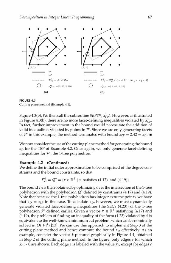
P1: shibuAugust 23, 2005 10:18 1914 1914˙CH04


(a) (b)

PP′

P0O = Q′ ∩ Q′′

x0CP =(2.25,2.75)

PP′

P1O = P0

O ∩ x ∈ Rn | 3x1 – x2 ≥ 5

x1CP =( 2.42, 2.25)

(2,1) (2, 1)

FIGURE 4.3Cutting plane method (Example 4.1).

Figure 4.3(b). We then call the subroutine SEP(P , x1CP). However, as illustrated

in Figure 4.3(b), there are no more facet-defining inequalities violated by x1CP.

In fact, further improvement in the bound would necessitate the addition ofvalid inequalities violated by points inP ′. Since we are only generating facetsof P ′ in this example, the method terminates with bound zCP = 2.42 = zD.

We now consider the use of the cutting plane method for generating the boundzD for the TSP of Example 4.2. Once again, we only generate facet-defininginequalities for P ′, the 1-tree polyhedron.

Example 4.2 (Continued)We define the initial outer approximation to be comprised of the degree con-straints and the bound constraints, so that

P0O = Q′′ = x ∈ RE | x satisfies (4.17) and (4.19).

The bound zD is then obtained by optimizing over the intersection of the 1-treepolyhedron with the polyhedron Q′′ defined by constraints (4.17) and (4.19).Note that because the 1-tree polyhedron has integer extreme points, we havethat zD = zLP in this case. To calculate zD, however, we must dynamicallygenerate violated facet-defining inequalities (the SECs (4.23)) of the 1-treepolyhedron P ′ defined earlier. Given a vector x ∈ RE satisfying (4.17) and(4.19), the problem of finding an inequality of the form (4.23) violated by x isequivalent to the well-known minimum cut problem, which can be nominallysolved in O(|V|4) [53]. We can use this approach to implement Step 3 of thecutting plane method and hence compute the bound zD effectively. As anexample, consider the vector x pictured graphically in Figure 4.4, obtainedin Step 2 of the cutting plane method. In the figure, only edges e for whichxe > 0 are shown. Each edge e is labeled with the value xe , except for edges e

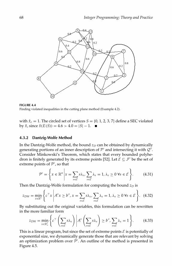
P1: shibuAugust 23, 2005 10:18 1914 1914˙CH04


0

1

2

0.6

3

0.2

0.8

0.2

4

5

6

0.8

7

0.8

8

9

0.6

10

11

0.4

0.2

12

0.2

0.20.2

130.4

0.60.8

14

0.6

0.2

0.2

15

0.2

0.2

0.2

0.80.6

FIGURE 4.4Finding violated inequalities in the cutting plane method (Example 4.2).

with xe = 1. The circled set of vertices S = 0, 1, 2, 3, 7 define a SEC violatedby x, since x(E(S)) = 4.6 > 4.0 = |S| − 1.

4.3.2 Dantzig-Wolfe Method

In the Dantzig-Wolfe method, the bound zD can be obtained by dynamicallygenerating portions of an inner description of P ′ and intersecting it with Q′′.Consider Minkowski’s Theorem, which states that every bounded polyhe-dron is finitely generated by its extreme points [52]. Let E ⊆ F ′ be the set ofextreme points of P ′, so that

P ′ =

x ∈ Rn

∣∣∣∣∣x =∑s∈E

sλs ,∑s∈E

λs = 1, λs ≥ 0 ∀s ∈ E

. (4.31)

Then the Dantzig-Wolfe formulation for computing the bound zD is

zDW = minx∈Rn

cx

∣∣∣∣∣A′′x ≥ b ′′, x =∑s∈E

sλs ,∑s∈E

λs = 1, λs ≥ 0 ∀s ∈ E

. (4.32)

By substituting out the original variables, this formulation can be rewrittenin the more familiar form

zDW = minλ∈RE+

c(∑

s∈Esλs

)∣∣∣∣∣A′′(∑

s∈Esλs

)≥ b ′′,

∑s∈E

λs = 1

. (4.33)

This is a linear program, but since the set of extreme points E is potentially ofexponential size, we dynamically generate those that are relevant by solvingan optimization problem over P ′. An outline of the method is presented inFigure 4.5.

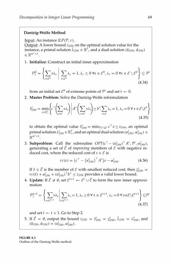
P1: shibuAugust 23, 2005 10:18 1914 1914˙CH04


Dantzig-Wolfe Method

Input: An instance ILP(P , c).Output: A lower bound zDW on the optimal solution value for theinstance, a primal solution λDW ∈ RE , and a dual solution (uDW, αDW)

∈ Rm′′+1.

1. Initialize: Construct an initial inner approximation

P0I =

∑s∈E0

sλs

∣∣∣∣∣∑s∈E0

λs = 1, λs ≥ 0 ∀s ∈ E0, λs = 0 ∀s ∈ E \ E0

⊆ P ′

(4.34)

from an initial set E0 of extreme points of P ′ and set t ← 0.2. Master Problem: Solve the Dantzig-Wolfe reformulation

ztDW = min

λ∈RE+

c(∑

s∈Esλs

)∣∣∣∣∣A′′(∑

s∈Esλs

)≥ b ′′,

∑s∈E

λs = 1, λs = 0 ∀ s ∈ E\E t

(4.35)

to obtain the optimal value ztDW = minP t

I ∩Q′′ cx ≥ zDW, an optimalprimal solution λt

DW ∈RE+, and an optimal dual solution (utDW, αt

DW) ∈R

m′′+1.3. Subproblem: Call the subroutine OPT(c− (ut

DW) A′′, P ′, αtDW),

generating a set of E of improving members of E with negative re-duced cost, where the reduced cost of s ∈ E is

rc(s) = (c − (utDW

) A′′)s − αtDW. (4.36)

If s ∈ E is the member of E with smallest reduced cost, then ztDW =

rc(s) + αtDW + (ut

DW)b ′′ ≤ zDW provides a valid lower bound.4. Update: If E = ∅, set E t+1 ← E t ∪ E to form the new inner approxi-

mation

P t+1I =

∑s∈E t+1

sλs

∣∣∣∣∣∑

s∈E t+1

λs = 1, λs ≥ 0 ∀ s ∈ E t+1, λs = 0 ∀ s∈E\E t+1

⊆P ′

(4.37)

and set t ← t + 1. Go to Step 2.5. If E = ∅, output the bound zDW = zt

DW = ztDW, λDW = λt

DW, and(uDW, αDW) = (ut

DW, αtDW).

FIGURE 4.5Outline of the Dantzig-Wolfe method.

P1: shibuAugust 23, 2005 10:18 1914 1914˙CH04


In Step 2, we solve the master problem, which is a restricted linear programobtained by substituting E t for E in (4.33). In Section 4.6, we discuss severalalternatives for solving this LP. In any case, solving it results in a primalsolution λt

DW, and a dual solution consisting of the dual multipliers utDW on the

constraints corresponding to [A′′, b ′′] and the multiplier αtDW on the convexity

constraint. The dual solution is needed to generate the improving columns inStep 3. In each iteration, we are generating an inner approximation, P t

I ⊆ P ′,the convex hull of E t. Thus P t

I ∩Q′′ may or may not contain P and the boundreturned from the master problem in Step 2, zt

DW, provides an upper boundon zDW. Nonetheless, it is easy to show (see Section 4.3.3) that an optimalsolution to the subproblem solved in Step 3 yields a valid lower bound. Inparticular, if s is a member of E with the smallest reduced cost in Step 3, then

ztDW = cs + (ut

DW

)(b ′′ − A′′s) (4.38)

is a valid lower bound. This means that, in contrast to the cutting planemethod, where a valid lower bound is always available, the Dantzig-Wolfemethod only yields a valid lower bound when the subproblem is solved tooptimality, i.e., the optimization version is solved, as opposed to the decisionversion. This need not be done in every iteration, as described below.

In Step 3, we search for improving members of E , where, as in the previoussection, this means members that when added to E t yield an improved bound.It is less clear here, however, which bound we would like to improve, zt

DW orzt

DW. A necessary condition for improving ztDW is the generation of a column

with negative reduced cost. In fact, if one considers (4.38), it is clear that thiscondition is also necessary for improvement of zt

DW. However, we point outagain that the subproblem must be solved to optimality in order to updatethe bound zt

DW. In either case, however, we are looking for members of E withnegative reduced cost. If one or more such members exist, we add them to E t

and iterate.An area that deserves some deeper investigation is the relationship between

the solution obtained by solving the reformulation (4.35) and the solution thatwould be obtained by solving an LP directly over P t

I ∩Q′′ with the objectivefunction c. Consider the primal optimal solution λt

DW, which we refer to as anoptimal decomposition. If we combine the members of E t using λt

DW to obtainan optimal fractional solution

xtDW =

∑s∈E t

s(λt

DW

)s , (4.39)

then we see that ztDW = cxt

DW. In fact, xtDW ∈ P t

I ∩Q′′ is an optimal solutionto the linear program solved directly over P t

I ∩Q′′ with objective function c.The optimal fractional solution plays an important role in the integrated

methods to be introduced later. To illustrate the Dantzig-Wolfe method andthe role of the optimal fractional solution in the method, we show how toapply it to generate the bound zD for the ILP of Example 4.1.

P1: shibuAugust 23, 2005 10:18 1914 1914˙CH04


′⊂ P)2Ev(on=cI2P

′⊂ P)1Ev(on=cI1P′⊂)0Ev(on=cI

0P

25).2,42.2= (DW2x

′PP

′′Q

4),3= (s

86).1,64.2= (DW1x

′PP

′′Q′′Q

= (2,1)s

2),25.4= (DW0x

1),(2

1),(21),(2

”Au–c

”Au–c

c ”Au–c

′PP

(c)

(b)(a)

P

FIGURE 4.6Dantzig-Wolfe method (Example 4.1).

Example 4.1 (Continued)For the purposes of illustration, we begin with a randomly generated initialset of points E0 = (4, 1), (5, 5). Taking their convex hull, we form the initialinner approximation P0

I = conv(E0), as illustrated in Figure 4.6(a).Iteration 0. Solving the master problem with inner polyhedron P0

I , we ob-tain an optimal primal solution (λ0

DW)(4,1) = 0.75, (λ0DW)(5,5) = 0.25, x0

DW =(4.25, 2), and bound z0

DW = 4.25. Since constraint (4.12) is binding at x0DW, the

only nonzero component of u0DW is (u0

DW)(4.12) = 0.28, while the dual variableassociated with the convexity constraint has value α0

DW = 4.17. All other dualvariables have value zero. Next, we search for an extreme point of P ′ with

P1: shibuAugust 23, 2005 10:18 1914 1914˙CH04


negative reduced cost, by solving the subproblem OPT(c − P ′, (utDW) A′′,

α0DW). From Figure 4.6(a), we see that s = (2, 1). This gives a valid lower bound

z0DW = 2.03. We add the corresponding column to the restricted master and

set E1 = E0 ∪ (2, 1).Iteration 1. The next iteration is depicted in Figure 4.6(b). First, we solve themaster problem with inner polyhedron P1

I = conv(E1) to obtain (λ1DW)(5,5) =

0.21, (λ1DW)(2,1) = 0.79, x1

DW = (2.64, 1.86), and bound and z1DW = 2.64. This

also provides the dual solution (u1DW)(4.13) = 0.43 and α1

DW = 0.71 (all otherdual values are zero). Solving OPT(c−P ′, u1

DW A′′, α1DW), we obtain s = (3, 4),

and z1DW = 1.93. We add the corresponding column to the restricted master

and set E2 = E1 ∪ (3, 4).Iteration 2. The final iteration is depicted in Figure 4.6(c). Solving the masterproblem once more with inner polyhedron P2

I = conv(E2), we obtain(λ2

DW)(2,1) = 0.58 and (λ2DW)(3,4) = 0.42, x2

DW = (2.42, 2.25), and bound z2DW =

2.42. This also provides the dual solution (u2DW)(4.14) = 0.17 and α2

DW = 0.83.Solving OPT(c −P ′, u2

DW A′′, α2DW), we conclude that E = ∅. We therefore ter-

minate with the bound zDW = 2.42 = zD.

As a further brief illustration, we return to the TSP example introduced earlier.

Example 4.2 (Continued)As we noted earlier, the Minimum 1-Tree Problem can be solved by comput-ing a minimum cost spanning tree on vertices V \ 0, and then adding twocheapest edges incident to vertex 0. This can be done in O(|E | log |V|) usingstandard algorithms. In applying the Dantzig-Wolfe method to compute zD

using the decomposition described earlier, the subproblem to be solved inStep 3 is a Minimum 1-Tree Problem. Because we can solve this problem ef-fectively, we can apply the Dantzig-Wolfe method in this case. As an exampleof the result of solving the Dantzig-Wolfe master problem (4.35), Figure 4.7depicts an optimal fractional solution (a) to a Dantzig-Wolfe master LP andthe six extreme points in Figure 4.7(b to g) of the 1-tree polyhedron P ′, withnonzero weight comprising an optimal decomposition. We return to this fig-ure later in Section 4.4.

Now consider the set S(u, α), defined as

S(u, α) = s ∈ E | (c − u A′′)s = α, (4.40)

where u ∈ Rm′′and α ∈ R. The set S(ut

DW, αtDW) is the set of members of E

with reduced cost zero at optimality for (4.35) in iteration t. It follows thatconv(S(ut

DW, αtDW)) is in fact the face of optimal solutions to the linear pro-

gram solved overP tI with objective function c −u A′′. This line of reasoning

culminates in the following theorem tying together the set S(utDW, αt

DW) de-fined above, the vector xt

DW, and the optimal face of solutions to the LP overthe polyhedron P t

I ∩Q′′.

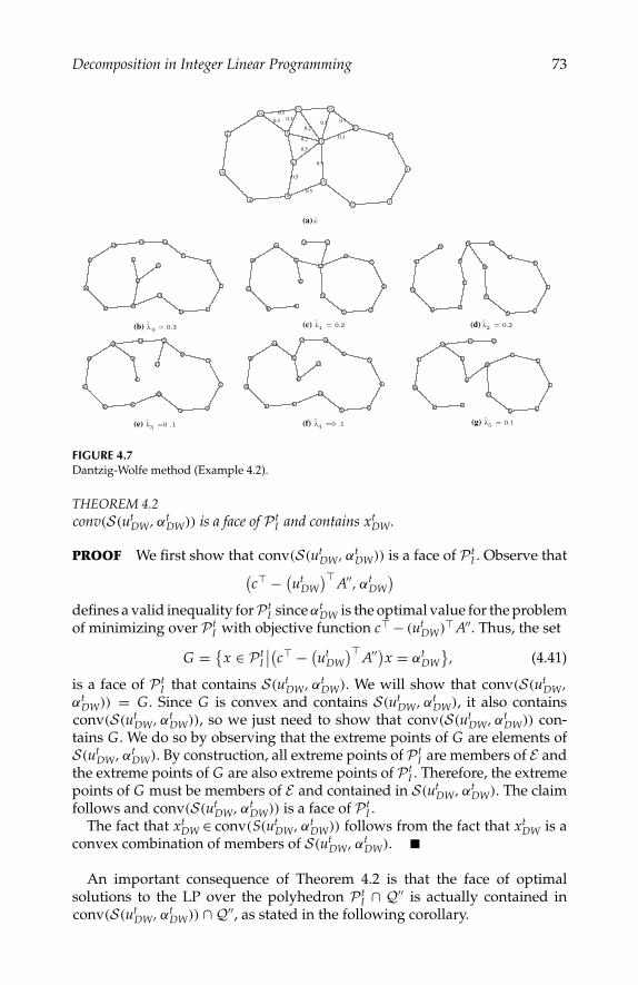
P1: shibuAugust 23, 2005 10:18 1914 1914˙CH04


000

0 0 0

0

121314

15

11

111

1 1 1

1

222

2 2 2

2

333

3 3 3

3

444

4 4 4

4

555

5 5 5

5

666

6 6 6

6

777

7 7 7

7

888

8 8 8

8

10

999

9 9 9

9

1010

1010

11 1111

1111

12 12

12 12

1313

13 13

14 14

14 14

15

15 15

15

0.5

0.5

0.5

0.5

0.5

0.5

0.2

0.3 0.7

0.3

0.3

0.2

(a)x

(b) λ 0 = 0.3 (c) λ1 = 0.2 (d) λ2 = 0.2

(e) λ3 =0 .1 (f) λ4 =0 .1 (g) λ5 = 0.1

ˆ

10

121314

15

10

121314

15

11

FIGURE 4.7Dantzig-Wolfe method (Example 4.2).

THEOREM 4.2conv(S(ut

DW, αtDW)) is a face of P t

I and contains xtDW.

PROOF We first show that conv(S(utDW, αt

DW)) is a face of P tI . Observe that(

c − (utDW

) A′′, αtDW

)defines a valid inequality forP t

I since αtDW is the optimal value for the problem

of minimizing over P tI with objective function c − (ut

DW) A′′. Thus, the set

G = x ∈ P tI

∣∣(c − (utDW

) A′′)x = αtDW

, (4.41)

is a face of P tI that contains S(ut

DW, αtDW). We will show that conv(S(ut

DW,αt

DW)) = G. Since G is convex and contains S(utDW, αt

DW), it also containsconv(S(ut

DW, αtDW)), so we just need to show that conv(S(ut

DW, αtDW)) con-

tains G. We do so by observing that the extreme points of G are elements ofS(ut

DW, αtDW). By construction, all extreme points of P t

I are members of E andthe extreme points of G are also extreme points of P t

I . Therefore, the extremepoints of G must be members of E and contained in S(ut

DW, αtDW). The claim

follows and conv(S(utDW, αt

DW)) is a face of P tI .

The fact that xtDW ∈ conv(S(ut

DW, αtDW)) follows from the fact that xt

DW is aconvex combination of members of S(ut

DW, αtDW).

An important consequence of Theorem 4.2 is that the face of optimalsolutions to the LP over the polyhedron P t

I ∩ Q′′ is actually contained inconv(S(ut

DW, αtDW)) ∩Q′′, as stated in the following corollary.

P1: shibuAugust 23, 2005 10:18 1914 1914˙CH04


COROLLARY 4.2If F is the face of optimal solutions to the linear program solved directly overP t

I ∩Q′′

with objective function vector c, then F ⊆ conv(S(utDW, αt

DW)) ∩Q′′.

PROOF Let x ∈ F be given. Then we have that x ∈ P tI ∩ Q′′ by definition,

and

c x = αtDW + (ut

DW

)b ′′ = αtDW + (ut

DW

) A′′ x, (4.42)

where the first equality in this chain is a consequence of strong duality andthe last is a consequence of complementary slackness. Hence, it follows that(c − (ut

DW) A′′)x = αtDW and the result is proven.

Hence, each iteration of the method not only produces the primal solu-tion xt

DW ∈ P tI ∩ Q′′, but also a dual solution (ut

DW, αtDW) that defines a face

conv(S(utDW, αt

DW)) of P tI that contains the entire optimal face of solutions to

the LP solved directly overP tI ∩Q′′ with the original objective function vector c.

When no column with negative reduced cost exists, the two bounds must beequal to zD and we stop, outputting both the primal solution λDW, and the dualsolution (uDW, αDW). It follows from the results proven above that in the finaliteration, any column of (4.35) with reduced cost zero must in fact have a costof αDW = zD − u

DWb ′′ when evaluated with respect to the modified objectivefunction c − u

DW A′′. In the final iteration, we can therefore strengthen thestatement of Theorem 4.2, as follows.

THEOREM 4.3conv(S(uDW, αDW)) is a face of P ′ and contains xDW.

The proof follows along the same lines as Theorem 4.2. As before, we can alsostate the following important corollary.

COROLLARY 4.3If F is the face of optimal solutions to the linear program solved directly over P ′ ∩Q′′

with objective function vector c, then F ⊆ conv(S(uDW, αDW)) ∩Q′′.

Thus, conv(S(uDW, αDW)) is actually a face of P ′ that contains xDW and theentire face of optimal solutions to the LP solved over P ′ ∩Q′′ with objectivefunction c. This fact provides strong intuition regarding the connection be-tween the Dantzig-Wolfe method and the cutting plane method and allowsus to regard Dantzig-Wolfe decomposition as either a procedure for produc-ing the bound zD = c xDW from primal solution information or the boundzD = cs + u

DW(b ′′ − A′′s), where s is any member of S(uDW, αDW), from dualsolution information. This fact is important in the next section, as well as laterwhen we discuss integrated methods.

The exact relationship between S(uDW, αDW), the polyhedron P ′ ∩Q′′, andthe face F of optimal solutions to an LP solved over P ′ ∩ Q′′ can vary fordifferent polyhedra and even for different objective functions. Figure 4.8

P1: shibuAugust 23, 2005 10:18 1914 1914˙CH04


FIGURE 4.8The relationship of P ′ ∩Q′′, conv(S(uDW, αDW)) ∩Q′′, and the face F .

shows the polyhedra of Example 4.1 with three different objective functionsindicated. The convex hull of S(uDW, αDW) is typically a proper face ofP ′, butit is possible for xDW to be an inner point of P ′, in which case we have thefollowing result.

P1: shibuAugust 23, 2005 10:18 1914 1914˙CH04


THEOREM 4.4If xDW is an inner point of P ′, then conv(S(uDW, αDW)) = P ′.

PROOF We prove the contrapositive. Suppose conv(S(uDW, αDW)) is aproper face of P ′. Then there exists a facet-defining valid inequality (a, β) ∈R

n+1 such that conv(S(uDW, αDW)) ⊆ x ∈ Rn | ax = β. By Theorem 4.3,

xDW ∈ conv(S(uDW, αDW)) and xDW therefore cannot satisfy the definition ofan inner point.

In this case, illustrated graphically in Figure 4.8(a) with the polyhedra fromExample 4.1, zDW = zLP and Dantzig-Wolfe decomposition does not improvethe bound. All columns of the Dantzig-Wolfe LP have reduced cost zero andany member of E can be given positive weight in an optimal decomposition.A necessary condition for an optimal fractional solution to be an inner pointof P ′ is that the dual value of the convexity constraint in an optimal solutionto the Dantzig-Wolfe LP be zero. This condition indicates that the chosenrelaxation may be too weak.

A second case of potential interest is when F = conv(S(uDW, αDW)) ∩ Q′′,illustrated graphically in Figure 4.8(b). In this case, all constraints of theDantzig-Wolfe LP other than the convexity constraint must have dual valuezero, since removing them does not change the optimal solution value. Thiscondition can be detected by examining the objective function values of themembers of E with positive weight in the optimal decomposition. If they areall identical, any such member that is contained in Q′′ (if one exists) mustbe optimal for the original ILP, since it is feasible and has objective functionvalue equal to zIP. The more typical case, in which F is a proper subset ofconv(S(uDW, αDW)) ∩Q′′, is shown in Figure 4.8(c).

4.3.3 Lagrangian Method

The Lagrangian method [14, 22] is a general approach for computing zD

that is closely related to the Dantzig-Wolfe method, but is focused primar-ily on producing dual solution information. The Lagrangian method can beviewed as a method for producing a particular face of P ′, as in the Dantzig-Wolfe method, but no explicit approximation of P ′ is maintained. Althoughthere are implementations of the Lagrangian method that do produce ap-proximate primal solution information similar to the solution informationthat the Dantzig-Wolfe method produces (see Section 4.3.2), our viewpointis that the main difference between the Dantzig-Wolfe method and the La-grangian method is the type of solution information they produce. This dis-tinction is important when we discuss integrated methods in Section 4.4.When exact primal solution information is not required, faster algorithmsfor determining the dual solution are possible. By employing a Lagrangianframework instead of a Dantzig-Wolfe framework, we can take advantage ofthis fact.

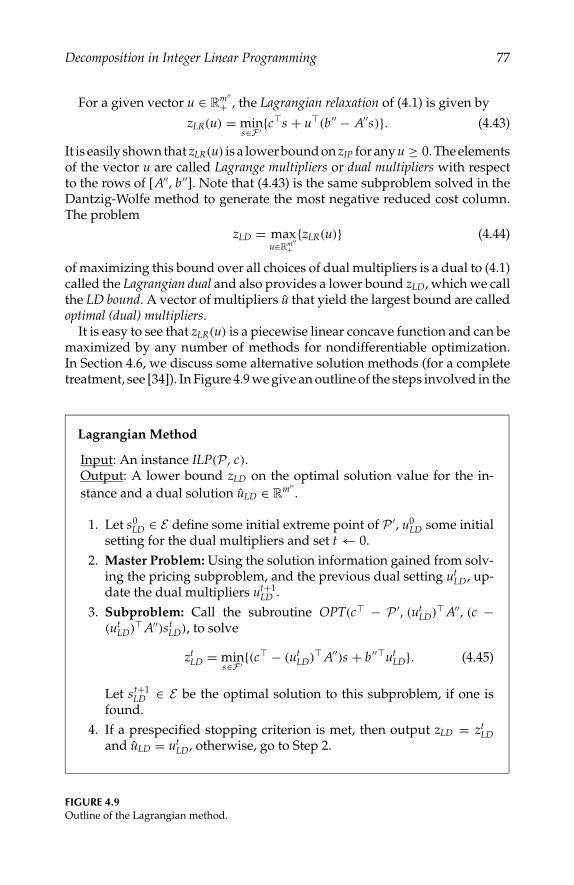
P1: shibuAugust 23, 2005 10:18 1914 1914˙CH04


For a given vector u ∈ Rm′′+ , the Lagrangian relaxation of (4.1) is given by

zLR(u) = mins∈F ′

cs + u(b ′′ − A′′s). (4.43)

It is easily shown that zLR(u) is a lower bound on zIP for any u ≥ 0. The elementsof the vector u are called Lagrange multipliers or dual multipliers with respectto the rows of [A′′, b ′′]. Note that (4.43) is the same subproblem solved in theDantzig-Wolfe method to generate the most negative reduced cost column.The problem

zLD = maxu∈Rm′′

+zLR(u) (4.44)

of maximizing this bound over all choices of dual multipliers is a dual to (4.1)called the Lagrangian dual and also provides a lower bound zLD, which we callthe LD bound. A vector of multipliers u that yield the largest bound are calledoptimal (dual) multipliers.

It is easy to see that zLR(u) is a piecewise linear concave function and can bemaximized by any number of methods for nondifferentiable optimization.In Section 4.6, we discuss some alternative solution methods (for a completetreatment, see [34]). In Figure 4.9 we give an outline of the steps involved in the

Lagrangian Method

Input: An instance ILP(P , c).Output: A lower bound zLD on the optimal solution value for the in-stance and a dual solution uLD ∈ Rm′′

.

1. Let s0LD ∈ E define some initial extreme point of P ′, u0

LD some initialsetting for the dual multipliers and set t ← 0.

2. Master Problem: Using the solution information gained from solv-ing the pricing subproblem, and the previous dual setting ut

LD, up-date the dual multipliers ut+1

LD .3. Subproblem: Call the subroutine OPT(c − P ′, (ut

LD) A′′, (c −(ut

LD) A′′)stLD), to solve

ztLD = min

s∈F ′(c − (ut

LD) A′′)s + b ′′utLD. (4.45)

Let st+1LD ∈ E be the optimal solution to this subproblem, if one is

found.4. If a prespecified stopping criterion is met, then output zLD = zt

LDand uLD = ut

LD, otherwise, go to Step 2.

FIGURE 4.9Outline of the Lagrangian method.

P1: shibuAugust 23, 2005 10:18 1914 1914˙CH04


Lagrangian method. As in Dantzig-Wolfe, the main loop involves updatingthe dual solution and then generating an improving member of E by solvinga subproblem. Unlike the Dantzig-Wolfe method, there is no approximationand hence no update step, but the method can nonetheless be viewed in thesame frame of reference.

To more clearly see the connection to the Dantzig-Wolfe method, considerthe dual of the Dantzig-Wolfe LP (4.33),

zDW = maxα∈R,u∈Rm′′

+α + b ′′u | α ≤ (c − u A′′)s ∀s ∈ E. (4.46)

Letting η = α + b ′′u and rewriting, we see that

zDW = maxη∈R,u∈Rm′′

+η | η ≤ (c − u A′′)s + b ′′u ∀s ∈ E (4.47)

= maxη∈R,u∈Rm′′

+min

s∈E(c − u A′′)s + b ′′u = zLD. (4.48)

Thus, we have that zLD = zDW and that (4.44) is another formulation forthe problem of calculating zD. It is also interesting to observe that the setS(ut

LD, ztLD −b ′′ut

LD) is the set of alternative optimal solutions to the subprob-lem solved at iteration t in Step 3. The following theorem is a counterpart toTheorem 4.3 that follows from this observation.

THEOREM 4.5conv(S(uLD, zLD − b ′′uLD)) is a face of P ′. Also, if F is the face of optimal solutionsto the linear program solved directly over P ′ ∩Q′′ with objective function vector c,then F ⊆ conv(S(uLD, zLD − b ′′uLD)) ∩Q′′.

Again, the proof is similar to that of Theorem 4.3. This shows that whilethe Lagrangian method does not maintain an explicit approximation, it doesproduce a face of P ′ containing the optimal face of solutions to the linearprogram solved over the approximation P ′ ∩Q′′.

4.4 Integrated Decomposition Methods

In Section 4.3, we demonstrated that traditional decomposition approachescan be viewed as utilizing dynamically generated polyhedral information toimprove the LP bound by either building an inner or an outer approximationof an implicitly defined polyhedron that approximatesP . The choice betweeninner and outer methods is largely an empirical one, but recent computationalresearch has favored outer methods. In what follows, we discuss three meth-ods for integrating inner and outer methods. In principle, this is not difficultto do and can result in bounds that are improved over those achieved byeither approach alone.

While traditional decomposition approaches build either an inner or anouter approximation, integrated decomposition methods build both an inner and

P1: shibuAugust 23, 2005 10:18 1914 1914˙CH04


an outer approximation. These methods follow the same basic loop as tra-ditional decomposition methods, except that the master problem is requiredto generate both primal and dual solution information and the subproblemcan be either a separation problem or an optimization problem. The first twotechniques we describe integrate the cutting plane method with either theDantzig-Wolfe method or the Lagrangian method. The third technique, de-scribed in Section 4.5, is a cutting plane method that uses an inner approxi-mation to perform separation.

4.4.1 Price and Cut

The integration of the cutting plane method with the Dantzig-Wolfe methodresults in a procedure that alternates between a subproblem that generatesimproving columns (the pricing subproblem) and a subproblem that gener-ates improving valid inequalities (the cutting subproblem). Hence, we callthe resulting method price and cut. When employed in a branch-and-boundframework, the overall technique is called branch, price, and cut. This methodhas already been studied previously by a number of authors [11, 12, 39, 60, 61]and more recently by Aragao and Uchoa [21].

As in the Dantzig-Wolfe method, the bound produced by price and cut canbe thought of as resulting from the intersection of two approximating polyhe-dra. However, the Dantzig-Wolfe method required one of these, Q′′, to havea short description. With integrated methods, both polyhedra can have de-scriptions of exponential size. Hence, price and cut allows partial descriptionsof both an inner polyhedron PI and an outer polyhedron PO to be generateddynamically. To optimize over the intersection ofPI andPO, we use a Dantzig-Wolfe reformulation as in (4.33), except that the [A′′, b ′′] is replaced by a matrixthat changes dynamically. The outline of this method is shown in Figure 4.10.

In examining the steps of this generalized method, the most interestingquestion that arises is how methods for generating improving columns andvalid inequalities translate to this new dynamic setting. Potentially trouble-some is the fact that column generation results in a reduction of the boundzt

PC produced by (4.51), while generation of valid inequalities is aimed atincreasing it. Recall again, however, that while it is the bound zt

PC that is di-rectly produced by solving (4.51), it is the bound zt

PC obtained by solving thepricing subproblem that one might claim is more relevant to our goal and thisbound can be potentially improved by generation of either valid inequalitiesor columns.

Improving columns can be generated in much the same way as they werein the Dantzig-Wolfe method. To search for new columns, we simply lookfor those that have negative reduced cost, where reduced cost is defined tobe the usual LP reduced cost with respect to the current reformulation. Hav-ing a negative reduced cost is still a necessary condition for a column to beimproving. However, it is less clear how to generate improving valid inequal-ities. Consider an optimal fractional solution xt

PC obtained by combining themembers of E according to weights yielded by the optimal decomposition λt

PC

P1: shibuAugust 23, 2005 10:18 1914 1914˙CH04


Price and Cut Method

Input: An instance ILP(P , c).Output: A lower bound zPC on the optimal solution value for the instance, aprimal solution xPC ∈ Rn, an optimal decomposition λPC ∈ RE , a dual solution(uPC , αPC ) ∈ Rmt+1, and the inequalities [DPC , dPC ] ∈ Rmt×(n+1).

1. Initialize: Construct an initial inner approximation

P0I =

∑s∈E0

sλs

∣∣∣∣∣∑s∈E0

λs = 1, λs ≥ 0 ∀s ∈ E0, λs = 0 ∀s ∈ E \ E0

⊆ P ′

(4.49)

from an initial set E0 of extreme points of P ′ and an initial outer approxi-mation

P0O = x ∈ Rn | D0x ≥ d0 ⊇ P , (4.50)

where D0 = A′′ and d0 = b ′′, and set t ← 0, m0 = m′′.

2. Master Problem: Solve the Dantzig-Wolfe reformulation

ztPC= min

λ ∈RE+

c(∑

s∈Esλs

)∣∣∣∣∣Dt

(∑s∈E

sλs

)≥dt,

∑s∈E

λs = 1, λs = 0 ∀s ∈ E \ E t

(4.51)

of the LP over the polyhedron P tI ∩P t

O to obtain the optimal value ztPC ,

an optimal primal solution λtPC ∈RE , an optimal fractional solution xt

PC =∑s∈E s(λt

PC )s , and an optimal dual solution (utPC , αt

PC ) ∈ Rmt+1.

3. Do either (a) or (b).(a) Pricing Subproblem and Update: Call the subroutine OPT

(c − P ′, (utPC ) Dt, αt

PC ), generating a set E of improving mem-bers of E with negative reduced cost (defined in Figure 4.5). IfE = ∅, set E t+1 ← E t ∪ E to form a new inner approximation P t+1

I .If s ∈ E is the member of E with smallest reduced cost, thenzt

PC = rc(s) + αtPC + (dt)ut

PC provides a valid lower bound. Set[Dt+1, dt+1] ← [Dt, dt], P t+1

O ←P tO, mt+1 ← mt , t ← t + 1, and go to

Step 2.

(b) Cutting Subproblem and Update: Call the subroutine SEP(P , xt

PC ) to generate a set of improving valid inequalities [D, d] ∈R

m×n+1 for P , violated by xtPC . If violated inequalities were found,

set [Dt+1, dt+1] ← [Dt dt

D d

]to form a new outer approximation P t+1

O .Set mt+1 ← mt + m, E t+1 ← E t , P t+1

I ←P tI , t ← t + 1, and go to Step 2.

4. If E = ∅ and no valid inequalities were found, output the boundzPC = zt

PC = ztPC = cxt

PC , xPC = xtPC , λPC = λt

PC , (uPC , αPC ) = (utPC , αt

PC ),and [DPC , dPC ] = [Dt, dt].

FIGURE 4.10Outline of the price and cut method.

P1: shibuAugust 23, 2005 10:18 1914 1914˙CH04


in iteration t. Following a line of reasoning similar to that followed in ana-lyzing the results of the Dantzig-Wolfe method, we can conclude that xt

PC isin fact an optimal solution to an LP solved directly over P t

I ∩ P tO with ob-

jective function vector c and that therefore, it follows from Theorem 4.1 thatany improving inequality must be violated by xt

PC . It thus seems sensible toconsider separating xt

PC from P . This is the approach taken in the method ofFigure 4.10.

To demonstrate how the price and cut method works, we return toExample 4.1.

Example 4.1 (Continued)We pick up the example at the last iteration of the Dantzig-Wolfe method andshow how the bound can be further improved by dynamically generatingvalid inequalities.Iteration 0. Solving the master problem with E0 = (4, 1), (5, 5), (2, 1), (3, 4)and the initial inner approximation P0

I = conv(E0) yields (λ0PC)(2,1) = 0.58 and

(λ0PC)(3,4) = 0.42, x0

PC = (2.42, 2.25), bound z0PC = z0

PC = 2.42. Next, we solve thecutting subproblem SEP(P , x0

PC), generating facet-defining inequalities of Pthat are violated by x0

PC . One such facet-defining inequality, x1 ≥ 3, is illus-trated in Figure 4.11(a). We add this inequality to the current set D0 = [A′′, b ′′]to form a new outer approximation P1

O, defined by the set D1.Iteration 1. Solving the new master problem, we obtain an optimal primal so-lution (λ1

PC)(4,1) = 0.42, (λ1PC)(2,1) = 0.42, (λ1

PC)(3,4) = 0.17, x1PC = (3, 1.5), bound

z1PC = 3, as well as an optimal dual solution (u1

PC , α1PC). Next, we consider the

pricing subproblem. Since x1PC is in the interior ofP ′, every extreme point ofP ′

has reduced cost 0 by Theorem 4.4. Therefore, there are no negative reducedcost columns and we switch again to the cutting subproblem SEP(x1

PC , P).As illustrated in Figure 4.11(b), we find another facet-defining inequality ofP violated by x1

PC , x2 ≥ 2. We then add this inequality to form D2 and furthertighten the outer approximation, now P2

O.Iteration 2. In the final iteration, we solve the master problem again to obtain(λ2

PC)(4,1) = 0.33, (λ2PC)(2,1) = 0.33, (λ2

PC)(3,4) = 0.33, x2PC = (3, 2), bound z2

PC = 3.Now, since the primal solution is integral, and is contained in P ′ ∩ Q′′, weknow that z2

PC = zIP and we terminate.

Let us now return to the TSP example to further explore the use of the priceand cut method.

Example 4.2 (Continued)As described earlier, application of the Dantzig-Wolfe method along with the1-tree relaxation for the TSP allows us to compute the bound zD obtained byoptimizing over the intersection of the 1-tree polyhedron (the inner polyhe-dron) with the polyhedronQ′′ (the outer polyhedron) defined by constraints(4.17) and (4.19). With price and cut, we can further improve the bound by al-lowing both the inner and outer polyhedra to have large descriptions. For this

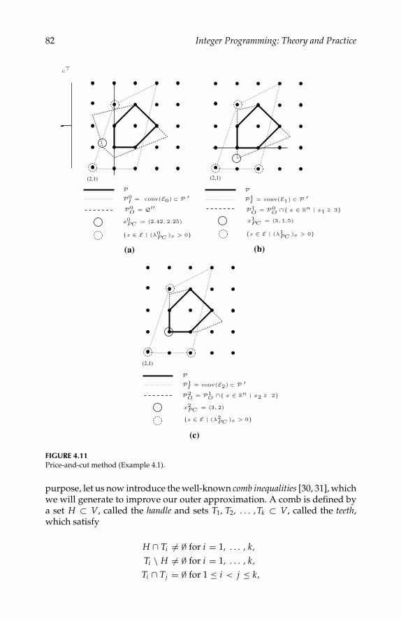
P1: shibuAugust 23, 2005 10:18 1914 1914˙CH04


′⊂ P)2Ev(on= cI1P

0>s)PC2λ(|∈ Es

0>s)PC1λ(|∈ Es0>s)PC

0λ(|∈ Es

′⊂ P)1Ev(on= cI1P′⊂ P)0Ev(on= cI

0P

2),3= (PC2x

2≥2x|nR∈x∩O

1P=O2P

P

5).1,3= (PC1x

3≥1x|nR∈x∩O

0P=O1P

P

25).2,42.2= (PC0x

′′Q=O0P

P

c

(2,1)

(2,1)(2,1)

(c)

(b)(a)

FIGURE 4.11Price-and-cut method (Example 4.1).

purpose, let us now introduce the well-known comb inequalities [30, 31], whichwe will generate to improve our outer approximation. A comb is defined bya set H ⊂ V, called the handle and sets T1, T2, . . . ,Tk ⊂ V, called the teeth,which satisfy

H ∩ Ti = ∅ for i = 1, . . . , k,

Ti \ H = ∅ for i = 1, . . . , k,

Ti ∩ Tj = ∅ for 1 ≤ i < j ≤ k,

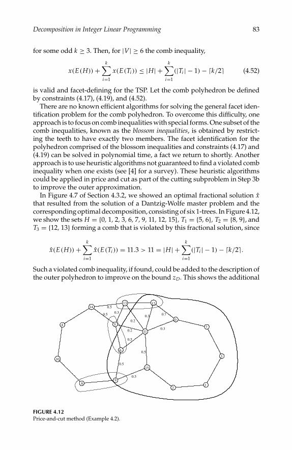
P1: shibuAugust 23, 2005 10:18 1914 1914˙CH04


for some odd k ≥ 3. Then, for |V| ≥ 6 the comb inequality,

x(E(H)) +k∑

i=1

x(E(Ti )) ≤ |H| +k∑

i=1

(|Ti | − 1) − k/2 (4.52)

is valid and facet-defining for the TSP. Let the comb polyhedron be definedby constraints (4.17), (4.19), and (4.52).

There are no known efficient algorithms for solving the general facet iden-tification problem for the comb polyhedron. To overcome this difficulty, oneapproach is to focus on comb inequalities with special forms. One subset of thecomb inequalities, known as the blossom inequalities, is obtained by restrict-ing the teeth to have exactly two members. The facet identification for thepolyhedron comprised of the blossom inequalities and constraints (4.17) and(4.19) can be solved in polynomial time, a fact we return to shortly. Anotherapproach is to use heuristic algorithms not guaranteed to find a violated combinequality when one exists (see [4] for a survey). These heuristic algorithmscould be applied in price and cut as part of the cutting subproblem in Step 3bto improve the outer approximation.

In Figure 4.7 of Section 4.3.2, we showed an optimal fractional solution xthat resulted from the solution of a Dantzig-Wolfe master problem and thecorresponding optimal decomposition, consisting of six 1-trees. In Figure 4.12,we show the sets H = 0, 1, 2, 3, 6, 7, 9, 11, 12, 15, T1 = 5, 6, T2 = 8, 9, andT3 = 12, 13 forming a comb that is violated by this fractional solution, since

x(E(H)) +k∑

i=1

x(E(Ti )) = 11.3 > 11 = |H| +k∑

i=1

(|Ti | − 1) − k/2.

Such a violated comb inequality, if found, could be added to the description ofthe outer polyhedron to improve on the bound zD. This shows the additional

0

121314

15

11

12

3

4 5

6

7

8

10

9

0.5

0.5

0.5

0.5

0.5

0.5

0.2

0.3 0.7

0.3

0.3

0.2

FIGURE 4.12Price-and-cut method (Example 4.2).

P1: shibuAugust 23, 2005 10:18 1914 1914˙CH04


power of price and cut over the Dantzig-Wolfe method. Of course, it shouldbe noted that it is also possible to generate such inequalities in the standardcutting plane method and to achieve the same bound improvement.

The choice of relaxation has a great deal of effect on the empirical be-havior of decomposition algorithms. In Example 4.2, we employed an innerpolyhedron with integer extreme points. With such a polyhedron, the inte-grality constraints of the inner polyhedron have no effect and zD = zLP. InExample 4.3, we consider a relaxation for which the bound zD may be strictlyimproved over zLP by employing an inner polyhedron that is not integral.

Example 4.3Let G be a graph as defined in Example 4.2 for the TSP. A 2-matching is asubgraph in which every vertex has degree two. Every TSP tour is hence a2-matching. The Minimum 2-Matching Problem is a relaxation of TSP whosefeasible region is described by the degree (4.17), bound (4.19), and integral-ity constraints (4.20) of the TSP. Interestingly, the 2-matching polyhedron,which is implicitly defined to be the convex hull of the feasible region justdescribed, can also be described by replacing the integrality constraints (4.20)with the blossom inequalities. Just as the SEC constraints provide a completedescription of the 1-tree polyhedron, the blossom inequalities (plus degreeand bound) constraints provide a complete description of the 2-matchingpolyhedron. Therefore, we could use this polyhedron as an outer approxima-tion to the TSP polyhedron. In [50], Muller-Hannemann and Schwartz presentseveral polynomial algorithms for optimizing over the 2-matching polyhe-dron. We can therefore also use the 2-matching relaxation in the context ofprice and cut to generate an inner approximation of the TSP polyhedron. Us-ing integrated methods, it would then be possible to simultaneously build upan outer approximation of the TSP polyhedron consisting of the SECs (4.18).Note that this simply reverses the roles of the two polyhedra from Example4.2 and thus would yield the same bound.

Figure 4.13 shows an optimal fractional solution arising from the solutionof the master problem and the 2-matchings with positive weight in a corre-sponding optimal decomposition. Given this fractional subgraph, we couldemploy the separation algorithm discussed in Example 4.2 of Section 4.3.1 togenerate the violated subtour S = 0, 1, 2, 3, 7.

Another approach to generating improving inequalities in price and cut isto try to take advantage of the information contained in the optimal decompo-sition to aid in the separation procedure. This information, though computedby solving (4.51) is typically ignored. Consider the fractional solution xt

PCgenerated in iteration t of the method in Figure 4.10. The optimal decompo-sition for the master problem in iteration t, λt

PC , provides a decomposition ofxt

PC into a convex combination of members of E . We refer to elements of E thathave a positive weight in this combination as members of the decomposition. Thefollowing theorem shows how such a decomposition can be used to derive

P1: shibuAugust 23, 2005 10:18 1914 1914˙CH04


000

0

1 11

1

2 22

2

0.6

3 3 3

3

4 44

0.2

5 55

0.8

6 66

0.2

77

4

7

5

8 8 8

6

9 9 9

0.8

10 10

7

10

0.8

11 11

8

11

12 12

9

12

0.6

131313

10

1414 14

11

1515 15

0.4

0.2

12

0.2

0.20.2

130.4

0.60.8

14

0.6

0.2

0.2

15

0.2

0.2

0.2

0.80.6

(b) λ0 = 0.2 (c) λ1 = 0.2 (d) λ2 = 0.6

(a) x

FIGURE 4.13Finding violated inequalities in price-and-cut (Example 4.3).

an alternate necessary condition for an inequality to be improving. Becausewe apply this theorem in a more general context later in the paper, we stateit in a general form.

THEOREM 4.6If x ∈ Rn violates the inequality (a, β) ∈ R(n+1) and λ ∈ RE+ is such that s∈E λs = 1and x = s∈Esλs , then there must exist an s ∈ E with λs > 0 such that s also violatesthe inequality (a, β) .

PROOF Let x ∈ Rn and (a, β) ∈ R(n+1) be given such that a x < β. Also, letλ ∈ RE+ be given such that s∈E λs = 1 and x = s∈Esλs . Suppose that as ≥ β

for all s ∈ E with λs > 0. Since s∈E λs = 1, we have a( s∈Esλs) ≥ β. Hence,a x = a( s∈Esλs) ≥ β, which is a contradiction.

In other words, an inequality can be improving only if it is violated by atleast one member of the decomposition. If I is the set of all improving in-equalities in iteration t, then the following corollary is a direct consequenceof Theorem 4.6.

COROLLARY 4.4I ⊆ V = (a, β) ∈ R(n+1) : as < β for some s ∈ E such that (λt

PC)s > 0.

P1: shibuAugust 23, 2005 10:18 1914 1914˙CH04


The importance of these results is that, in many cases, separation of mem-bers of F ′ from P is easier than separation of arbitrary real vectors. Thereare a number of well-known polyhedra for which the problem of separatingan arbitrary real vector is difficult, but the problem of separating a solutionto a given relaxation is easy. This concept is formalized in Section 4.5 andsome examples are discussed in Section 4.8. In Figure 4.14, we propose a newseparation procedure that can be embedded in price and cut that takes advan-tage of this fact. The procedure takes as input an arbitrary real vector x thathas been previously decomposed into a convex combination of vectors withknown structure. In price and cut, the arbitrary real vector is xt

PC and it is de-composed into a convex combination of members of E by solving the masterproblem (4.51). Rather than separating xt

PC directly, the procedure consistsof separating each one of the members of the decomposition in turn, thenchecking each inequality found for violation against xt

PC .The running time of this procedure depends in part on the cardinality

of the decomposition. Caratheodory’s Theorem assures us that there exists adecomposition with less than or equal to dim(P t

I )+1 members. Unfortunately,even if we limit our search to a particular known class of valid inequalities,the number of such inequalities violated by each member of D in Step 2 maybe extremely large and these inequalities may not be violated by xt

PC (such aninequality cannot be improving). Unless we enumerate every inequality in theset V from Corollary 4.4, either implicitly or explicitly, the procedure does notguarantee that an improving inequality will be found, even if one exists. Incases where examination of the setV in polynomial time is possible, the worst-case complexity of the entire procedure is polynomially equivalent to that ofoptimizing over P ′. Obviously, it is unlikely that the set V can be examined inpolynomial time in situations when separating xt

PC is itself an NP-completeproblem. In such cases, the procedure to select inequalities that are likely to

Separation Using a Decomposition

Input: A decomposition λ ∈ RE of x ∈ Rn.Output: A set [D, d] of potentially improving inequalities.

1. Form the set D = s ∈ E | λs > 0.2. For each s ∈ D, call the subroutine SEP(P , s) to obtain a set [D, d]

of violated inequalities.3. Let [D, d] be composed of the inequalities found in Step 2 that are

also violated by x, so that Dx < d.4. Return [D, d] as the set of potentially improving inequalities.

FIGURE 4.14Solving the cutting subproblem with the aid of a decomposition.

P1: shibuAugust 23, 2005 10:18 1914 1914˙CH04


be violated by xtPC in Step 2 is necessarily a problem-dependent heuristic. The

effectiveness of such heuristics can be improved in a number of ways, someof which are discussed in [57].

Note that members of the decomposition in iteration t must belong to theset S(ut

PC , αtPC), as defined by (4.40). It follows that the convex hull of the

decomposition is a subset of conv(S(utPC , αt

PC)) that contains xtPC and can

be thought of as a surrogate for the face of optimal solutions to an LP solveddirectly overP t

I ∩P tO with objective function vector c. Combining this corollary

with Theorem 4.1, we conclude that separation of S(utPC , αt

PC) from P is asufficient condition for an inequality to be improving. Although this sufficientcondition is difficult to verify in practice, it does provide additional motivationfor the method described in Figure 4.14.

Example 4.1 (Continued)Returning to the cutting subproblem in iteration 0 of the price and cut method,we have a decomposition x0

PC = (2.42, 2.25) = 0.58(2, 1) + 0.42(3, 4), as de-picted in Figure 4.11(a). Now, instead of trying to solve the subproblemSEP(P , x0

PC), we instead solve SEP(P , s), for each s ∈D= (2, 1), (3, 4). Inthis case, when solving the separation problem for s = (2, 1), we find the samefacet-defining inequality of P as we did by separating x0

PC directly.Similarly, in iteration 1, we have a decomposition of x2

PC = (3, 1.5) into a con-vex combination of D= (4, 1), (2, 1), (3, 4). Clearly, solving the separationproblem for either (2, 1) or (4, 1) produces the same facet-defining inequalityas with the original method.

Example 4.2 (Continued)Returning again to Example 4.2, recall the optimal fractional solution and thecorresponding optimal decomposition arising during solution of the TSP bythe Dantzig-Wolfe method in Figure 4.7. Figure 4.12 shows a comb inequalityviolated by this fractional solution. By Theorem 4.6, at least one of the mem-bers of the optimal decomposition shown in Figure 4.7 must also violate thisinequality. In fact, the member with index 0, also shown in Figure 4.15, is theonly such member. Note that the violation is easy to discern from the struc-ture of this integral solution. Let x ∈ 0, 1E be the incidence vector of a 1-tree.Consider a subset H of V whose induced subgraph in the 1-tree is a path withedge set P . Consider also an odd set O of edges of the 1-tree of cardinality atleast 3 and disjoint from P , such that each edge has one endpoint in H andone endpoint in V \ H. Taking the set H to be the handle and the endpoints ofeach member of O to be the teeth, it is easy to verify that the correspondingcomb inequality will be violated by the 1-tree, since

x(E(H)) +k∑

i=1

x(E(Ti )) = |H| − 1 +k∑

i=1

(|Ti | − 1) > |H| +k∑

i=1

(|Ti | − 1) − k/2.

Hence, searching for such configurations in the members of the decomposi-tion, as suggested in the procedure of Figure 4.14, may lead to the discovery

P1: shibuAugust 23, 2005 10:18 1914 1914˙CH04


0

0

121314

15

11

1

1

2

2

3

3

4

4

5

5

6

6

7

7

8

8

10

9

9

10

11

121314

15

0.50.5

0.5

0.5

0.5

0.5

0.2

0.3 0.7

0.3

0.3

0.2

(a) x

(b) λ0

FIGURE 4.15Using the optimal decomposition to find violated inequalities in price and cut (Example 4.2).

of comb inequalities violated by the optimal fractional solution. In this case,such a configuration does in fact lead to discovery of the previously indi-cated comb inequality. Note that we have restricted ourselves in the abovediscussion to the generation of blossom inequalities. The teeth, as well as thehandles can have more general forms that may lead to the discovery of moregeneral forms of violated combs.

Example 4.3 (Continued)Returning now to Example 4.3, recall the optimal fractional solution and thecorresponding optimal decomposition, consisting of the 2-matchings shownin Figure 4.13. Previously, we produced a set of vertices defining a SEC vio-lated by the fractional point by using a minimum cut algorithm with the opti-mal fractional solution as input. Now, let us consider applying the procedure

P1: shibuAugust 23, 2005 10:18 1914 1914˙CH04


of Figure 4.14 by examining the members of the decomposition in order to dis-cover inequalities violated by the optimal fractional solution. Let x ∈ 0, 1E

be the incidence vector of a 2-matching. If the corresponding subgraph doesnot form a tour, then it must be disconnected. The vertices correspondingto any connected component thus define a violated SEC. By determiningthe connected components of each member of the decomposition, it is easyto find violated SECs. In fact, for any 2-matching, every component of the2-matching forms a SEC that is violated by exactly 1. For the 2-matching cor-responding to s, we have x(E(S)) = |S| > |S| − 1. Figure 4.16(b) shows thethird member of the decomposition along with a violated SEC defined by one

0

0

1

1

2

2

0.6

3

3

4

0.2

5

0.8

6

0.2

4

7

5

6

8

0.8

9

7

10

0.8

8

11

9

12

0.6

13

10

14

11

0.4

15

0.2

12

0.2

0.20.2

130.4

0.60.8

14

0.6

0.2

0.2

15

0.2

0.2

0.2

0.80.6

(a) x

(b) λ2

FIGURE 4.16Using the optimal decomposition to find violated inequalities in price and cut (Example 4.3).

P1: shibuAugust 23, 2005 10:18 1914 1914˙CH04


of its components. This same SEC is also violated by the optimal fractionalsolution.

There are many variants of the price-and-cut method shown in Figure 4.10.Most significant is the choice of which subproblem to execute during Step 3. Itis easy to envision a number of heuristic rules for deciding this. For example,one obvious rule is to continue generating columns until no more are availableand then switch to valid inequalities for one iteration, then generate columnsagain until none are available. This can be seen as performing a “complete”dual solution update before generating valid inequalities. Further variantscan be obtained by not insisting on a “complete” dual update before solvingthe pricing problem [17, 29]. This rule could easily be inverted to generatevalid inequalities until no more are available and then generate columns. Ahybrid rule in which some sort of alternation occurs is a third option. Thechoice between these options is primarily empirical.

4.4.2 Relax and Cut

Just as with the Dantzig-Wolfe method, the Lagrangian method of Figure 4.9can be integrated with the cutting plane method to yield a procedure severalauthors have termed relax and cut. This is done in much the same fashionas in price and cut, with a choice in each iteration between solving a pric-ing subproblem and a cutting subproblem. In each iteration that the cuttingsubproblem is solved, the generated valid inequalities are added to the de-scription of the outer polyhedron, which is explicitly maintained as the algo-rithm proceeds. As with the traditional Lagrangian method, no explicit innerpolyhedron is maintained, but the algorithm can again be seen as one thatcomputes a face of the implicitly defined inner polyhedron that contains theoptimal face of solutions to a linear program solved over the intersection ofthe two polyhedra. When employed within a branch and bound framework,we call the overall method branch, relax, and cut.

An outline of the relax-and-cut method is shown in Figure 4.17. The ques-tion again arises as to how to ensure that the inequalities being generated inthe cutting subproblem are improving. In the case of the Lagrangian method,this is a much more difficult issue because we cannot assume the availabilityof the same primal solution information available within price and cut. Fur-thermore, we cannot verify the condition of Corollary 4.1, which is the bestavailable necessary condition for an inequality to be improving. Neverthe-less, some primal solution information is always available in the form of thesolution st

RC to the last pricing subproblem that was solved. Intuitively, sep-arating st

RC makes sense since the infeasibilities present in stRC may possibly

be removed through the addition of valid inequalities violated by stRC .

As with both the cutting plane and price-and-cut methods, the difficultyis that the valid inequalities generated by separating st

RC from P may notbe improving, as Guignard first observed in [33]. To deepen understandingof the potential effectiveness of the valid inequalities generated, we further

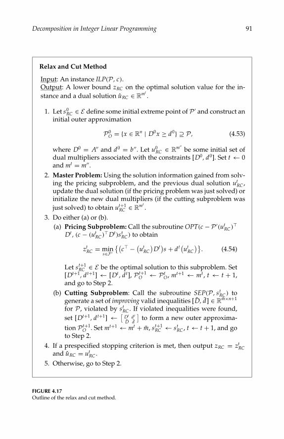
P1: shibuAugust 23, 2005 10:18 1914 1914˙CH04


Relax and Cut Method

Input: An instance ILP(P , c).Output: A lower bound zRC on the optimal solution value for the in-stance and a dual solution uRC ∈ Rmt

.

1. Let s0RC ∈ E define some initial extreme point of P ′ and construct an

initial outer approximation

P0O = x ∈ Rn | D0x ≥ d0 ⊇ P , (4.53)

where D0 = A′′ and d0 = b ′′. Let u0RC ∈ Rm′′

be some initial set ofdual multipliers associated with the constraints [D0, d0]. Set t ← 0and mt = m′′.

2. Master Problem: Using the solution information gained from solv-ing the pricing subproblem, and the previous dual solution ut

RC ,update the dual solution (if the pricing problem was just solved) orinitialize the new dual multipliers (if the cutting subproblem wasjust solved) to obtain ut+1

RC ∈ Rmt.

3. Do either (a) or (b).(a) Pricing Subproblem: Call the subroutine OPT(c −P ′(ut

RC)

Dt, (c − (utRC) Dt)st

RC) to obtain

ztRC = min

s∈F ′

(c − (ut

RC

)Dt)s + dt(ut

RC

). (4.54)

Let st+1RC ∈ E be the optimal solution to this subproblem. Set

[Dt+1, dt+1] ← [Dt, dt], P t+1O ← P t

O, mt+1 ← mt, t ← t + 1,and go to Step 2.

(b) Cutting Subproblem: Call the subroutine SEP(P , stRC) to

generate a set of improving valid inequalities [D, d] ∈ Rm×n+1

for P , violated by stRC . If violated inequalities were found,

set [Dt+1, dt+1] ← [Dt dt

D d

]to form a new outer approxima-

tion P t+1O . Set mt+1 ← mt + m, st+1

RC ← stRC , t ← t + 1, and go

to Step 2.4. If a prespecified stopping criterion is met, then output zRC = zt

RCand uRC = ut

RC .5. Otherwise, go to Step 2.

FIGURE 4.17Outline of the relax and cut method.

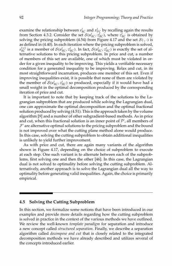
P1: shibuAugust 23, 2005 10:18 1914 1914˙CH04


examine the relationship between stRC and xt

PC by recalling again the resultsfrom Section 4.3.2. Consider the set S(ut

RC , ztRC), where zt

RC is obtained bysolving the pricing subproblem (4.54) from Figure 4.17 and the set S(·, ·) isas defined in (4.40). In each iteration where the pricing subproblem is solved,st+1

RC is a member of S(utRC , zt

RC). In fact, S(utRC , zt

RC) is exactly the set of al-ternative solutions to this pricing subproblem. In price and cut, a numberof members of this set are available, one of which must be violated in or-der for a given inequality to be improving. This yields a verifiable necessarycondition for a generated inequality to be improving. Relax and cut, in itsmost straightforward incarnation, produces one member of this set. Even ifimproving inequalities exist, it is possible that none of them are violated bythe member of S(ut

RC , ztRC) so produced, especially if it would have had a

small weight in the optimal decomposition produced by the correspondingiteration of price and cut.

It is important to note that by keeping track of the solutions to the La-grangian subproblem that are produced while solving the Lagrangian dual,one can approximate the optimal decomposition and the optimal fractionalsolution produced by solving (4.51). This is the approach taken by the volumealgorithm [9] and a number of other subgradient-based methods. As in priceand cut, when this fractional solution is an inner point of P ′, all members ofF ′ are alternative optimal solutions to the pricing subproblem and the boundis not improved over what the cutting plane method alone would produce.In this case, solving the cutting subproblem to obtain additional inequalitiesis unlikely to yield further improvement.

As with price and cut, there are again many variants of the algorithmshown in Figure 4.17, depending on the choice of subproblem to executeat each step. One such variant is to alternate between each of the subprob-lems, first solving one and then the other [46]. In this case, the Lagrangiandual is not solved to optimality before solving the cutting subproblem. Al-ternatively, another approach is to solve the Lagrangian dual all the way tooptimality before generating valid inequalities. Again, the choice is primarilyempirical.

4.5 Solving the Cutting Subproblem

In this section, we formalize some notions that have been introduced in ourexamples and provide more details regarding how the cutting subproblemis solved in practice in the context of the various methods we have outlined.We review the well-known template paradigm for separation and introducea new concept called structured separation. Finally, we describe a separationalgorithm called decompose and cut that is closely related to the integrateddecomposition methods we have already described and utilizes several ofthe concepts introduced earlier.

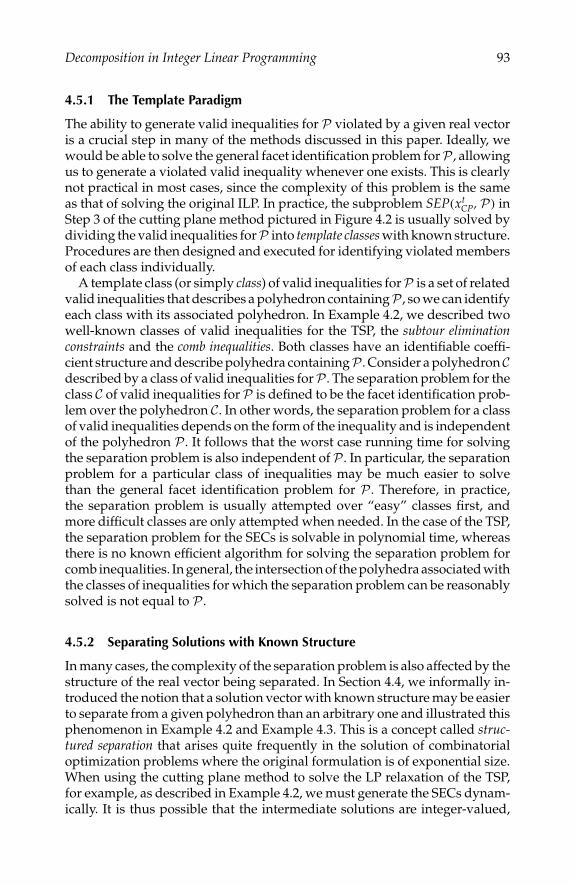
P1: shibuAugust 23, 2005 10:18 1914 1914˙CH04


4.5.1 The Template Paradigm

The ability to generate valid inequalities for P violated by a given real vectoris a crucial step in many of the methods discussed in this paper. Ideally, wewould be able to solve the general facet identification problem forP , allowingus to generate a violated valid inequality whenever one exists. This is clearlynot practical in most cases, since the complexity of this problem is the sameas that of solving the original ILP. In practice, the subproblem SEP(xt

CP, P) inStep 3 of the cutting plane method pictured in Figure 4.2 is usually solved bydividing the valid inequalities forP into template classes with known structure.Procedures are then designed and executed for identifying violated membersof each class individually.

A template class (or simply class) of valid inequalities forP is a set of relatedvalid inequalities that describes a polyhedron containingP , so we can identifyeach class with its associated polyhedron. In Example 4.2, we described twowell-known classes of valid inequalities for the TSP, the subtour eliminationconstraints and the comb inequalities. Both classes have an identifiable coeffi-cient structure and describe polyhedra containingP . Consider a polyhedronCdescribed by a class of valid inequalities forP . The separation problem for theclass C of valid inequalities forP is defined to be the facet identification prob-lem over the polyhedron C. In other words, the separation problem for a classof valid inequalities depends on the form of the inequality and is independentof the polyhedron P . It follows that the worst case running time for solvingthe separation problem is also independent of P . In particular, the separationproblem for a particular class of inequalities may be much easier to solvethan the general facet identification problem for P . Therefore, in practice,the separation problem is usually attempted over “easy” classes first, andmore difficult classes are only attempted when needed. In the case of the TSP,the separation problem for the SECs is solvable in polynomial time, whereasthere is no known efficient algorithm for solving the separation problem forcomb inequalities. In general, the intersection of the polyhedra associated withthe classes of inequalities for which the separation problem can be reasonablysolved is not equal to P .

4.5.2 Separating Solutions with Known Structure

In many cases, the complexity of the separation problem is also affected by thestructure of the real vector being separated. In Section 4.4, we informally in-troduced the notion that a solution vector with known structure may be easierto separate from a given polyhedron than an arbitrary one and illustrated thisphenomenon in Example 4.2 and Example 4.3. This is a concept called struc-tured separation that arises quite frequently in the solution of combinatorialoptimization problems where the original formulation is of exponential size.When using the cutting plane method to solve the LP relaxation of the TSP,for example, as described in Example 4.2, we must generate the SECs dynam-ically. It is thus possible that the intermediate solutions are integer-valued,

P1: shibuAugust 23, 2005 10:18 1914 1914˙CH04


but nonetheless not feasible because they violate some SEC that is not presentin the current approximation. When the current solution is optimal, however,it is easy to determine whether it violates a SEC — we simply examine theconnected components of the underlying support graph, as described earlier.This process can be done in O(|V|+ |E |) time. For an arbitrary real vector, theseparation problem for SECs is more difficult, taking O(|V|4) time.

It is also frequently the case that when applying a sequence of separationroutines for progressively more difficult classes of inequalities, routines forthe more difficult classes assume implicitly that the solution to be separatedsatisfies all inequalities of the the easier classes. In the case of the TSP, forinstance, any solution passed to the subroutine for separating the comb in-equalities is generally assumed to satisfy the degree and subtour eliminationconstraints. This assumption can allow the separation algorithms for subse-quent classes to be implemented more efficiently.

For the purposes of the present work, our main concern is with separat-ing solutions that are known to be integral, in particular, members of F ′. Inour framework, the concept of structured separation is combined with thetemplate paradigm in specifying template classes of inequalities for whichseparation of integral solutions is much easier, in a complexity sense, thanseparation of arbitrary real vectors over that same class. A number of ex-amples of problems and classes of valid inequalities for which this situationoccurs are examined in Section 4.8. We now examine a separation paradigmcalled decompose and cut that can take advantage of our ability to easily sepa-rate solutions with structure.

4.5.3 Decompose and Cut

The use of a decomposition to aid in separation, as is described in the proce-dure of Figure 4.14, is easy to extend to a traditional branch-and-cut frame-work using a technique we call decompose and cut, originally proposed in [56]and further developed in [40] and [57]. Suppose now that we are given an op-timal fractional solution xt

CP obtained during iteration t of the cutting planemethod and suppose that for a given s ∈ F ′, we can determine effectivelywhether s ∈ F and if not, generate a valid inequality (a, β) violated by s. Byfirst decomposing xt

CP (i.e., expressing xtCP as a convex combination of members

of E ⊆ F ′) and then separating each member of this decomposition from P inthe fashion described in Figure 4.14, we may be able to find valid inequalitiesfor P that are violated by xt

CP.The difficult step is finding the decomposition of xt

CP. This can be accom-plished by solving a linear program whose columns are the members of E ,as described in Figure 4.18. This linear program is reminiscent of (4.33) andin fact can be solved using an analogous column-generation scheme, as de-scribed in Figure 4.19. This scheme can be seen as the “inverse” of the methoddescribed in Section 4.4.1, since it begins with the fractional solution xt

CP andtries to compute a decomposition, instead of the other way around. By theequivalence of optimization and facet identification, we can conclude that the

P1: shibuAugust 23, 2005 10:18 1914 1914˙CH04


Separation in Decompose and Cut

Input: x ∈ Rn

Output: A valid inequality for P violated by x, if one is found.

1. Apply standard separation techniques to separate x. If one of thesereturns a violated inequality, then STOP and output the violatedinequality.

2. Otherwise, solve the linear program

maxλ∈RE+

0λ

∣∣∣∣∣∑s∈E

sλs = x,∑s∈E

λs = 1

, (4.55)

as in Figure 4.19.3. The result of Step 2 is either (1) a subset D of members of E partici-

pating in a convex combination of x, or (2) a valid inequality (a, β)

forP that is violated by x. In the first case, go to Step 4. In the secondcase, STOP and output the violated inequality.

4. Attempt to separate each member of D from P . For each inequalityviolated by a member of D, check whether it is also violated by x.If an inequality violated by x is encountered, STOP and output it.

FIGURE 4.18Separation in the decompose-and-cut method.

Column Generation in Decompose and Cut

Input: x ∈ Rn

Output: Either (1) a valid inequality for P violated by x; or (2) a subsetD of E and a vector λ ∈ RE+ such that s∈Dλss = x and s∈Dλs = 1.

2.0 Generate an initial subset E0 of E and set t ← 0.2.1 Solve (4.55), replacing E by E t. If this linear program is feasible, then

the elements of E t corresponding to the nonzero components of λ, thecurrent solution, comprise the set D, so STOP.

2.2 Otherwise, let (a, β) be a valid inequality for conv(E t) violated byx (i.e., the proof of infeasibility). Solve OPT(P ′, a , β) and let E be theresulting set of solutions. If E = ∅, then set E t+1 ← E t ∪ E , t → t + 1,and go to 2.1. Otherwise, (a, β) is an inequality valid for P ′ ⊇ P andviolated by x, so STOP.

FIGURE 4.19Column generation for the decompose-and-cut method.

P1: shibuAugust 23, 2005 10:18 1914 1914˙CH04


problem of finding a decomposition of xtCP is polynomially equivalent to that

of optimizing over P ′.Once the decomposition is found, it can be used as before to locate a violated

valid inequality. In contrast to price and cut, however, it is possible that xtCP ∈

P ′. This could occur, for instance, if exact separation methods for P ′ are tooexpensive to apply consistently. In this case, it is obviously not possible tofind a decomposition in Step 2 of Figure 4.18. The proof of infeasibility for thelinear program (4.55), however, provides an inequality separating xt

CP fromP ′ at no additional expense. Hence, even if we fail to find a decomposition,we still find an inequality valid for P and violated by xt

CP. This idea wasoriginally suggested in [56] and was further developed in [40]. A similarconcept was also discovered and developed independently by Applegate,et al. [3].

Applying decompose and cut in every iteration as the sole means of sep-aration is theoretically equivalent to price and cut. In practice, however,the decomposition is only computed when needed, i.e., when less expen-sive separation heuristics fail to separate the optimal fractional solution.This could give decompose and cut an advantage in terms of computationalefficiency. In other respects, the computations performed in each method aresimilar.

4.6 Solving the Master Problem

The choice of a proper algorithm for solving the master problem is importantfor these methods, both because a significant portion of the computationaleffort is spent solving the master problem and because the solver must becapable of returning the solution information required by the method. In thissection, we would like to briefly give the reader a taste for the issues involvedand summarize the existing methodology. The master problems we have dis-cussed are linear programs, or can be reformulated as linear programs. Hence,one option for solving them is to use either simplex or interior point methods.In the case of solving a Lagrangian dual, subgradient methods may also beemployed.

Simplex methods have the advantage of providing accurate primal solutioninformation. They are therefore well-suited for algorithms that utilize primalsolution information, such as price and cut. The drawback of these methodsis that updates to the dual solution at each iteration are relatively expensive.In their most straightforward implementations, they also tend to convergeslowly when used with column generation. This is primarily due to the factthat they produce basic (extremal) dual solutions, which tend to change sub-stantially from one iteration to the next, causing wide oscillations in the inputto the column-generation subproblem. This problem can be addressed by im-plementing one of a number of stabilization methods that prevent the dual

P1: shibuAugust 23, 2005 10:18 1914 1914˙CH04


solution from changing “too much” from one iteration to the next (for a sur-vey, see [43]).

Subgradient methods, on the other hand, do not produce primal solutioninformation in their most straightforward form, so they are generally mostappropriate for Lagrangian methods such as relax and cut. It is possible,however, to obtain approximate primal solutions from variants of subgradientsuch as the volume algorithm [9]. Subgradient methods also have convergenceissues without some form of stabilization. A recent class of algorithms thathas proven effective in this regard is bundle methods [18].

Interior point methods may provide a middle ground by providing accu-rate primal solution information and more stable dual solutions [28, 58]. Inaddition, hybrid methods that alternate between simplex and subgradientmethods for updating the dual solution have also shown promise [10, 36].

4.7 Software

The theoretical and algorithmic framework proposed in Section 4.3 to Section4.5 lends itself nicely to a wide-ranging and flexible generic software frame-work. All of the techniques discussed can be implemented by combining aset of basic algorithmic building blocks. DECOMP is a C++ framework de-signed with the goal of providing a user with the ability to easily utilizevarious traditional and integrated decomposition methods while requiringonly the provision of minimal problem-specific algorithmic components [25].With DECOMP, the majority of the algorithmic structure is provided as partof the framework, making it easy to compare various algorithms directly anddetermine which option is the best for a given problem setting. In addition,DECOMP is extensible — each algorithmic component can be overridden bythe user, if they so wish, in order to develop sophisticated variants of theaforementioned methods.

The framework is divided into two separate user interfaces, an applica-tions interface DecompApp, in which the user must provide implementationsof problem-specific methods (e.g., solvers for the subproblems), and an al-gorithms interface DecompAlgo, in which the user can modify DECOMP’sinternal algorithms, if desired. A DecompAlgo object provides implementa-tions of all of the methods described in Section 4.3 and Section 4.4, as well asoptions for solving the master problem, as discussed in Section 4.6. One im-portant feature of DECOMP is that the problem is always represented in theoriginal space, rather than in the space of a particular reformulation. The userhas only to provide subroutines for separation and column generation in theoriginal space without considering the underlying method. The frameworkperforms all of the necessary bookkeeping tasks, including automatic refor-mulation in the Dantzig-Wolfe master, constraint dualization for relax and cut,cut and variable pool management, as well as, row and column expansion.

P1: shibuAugust 23, 2005 10:18 1914 1914˙CH04


In order to develop an application, the user must provide implementationsof the following two methods:

• DecompApp::createCore(). The user must define the initial setof constraints [A′′, b ′′].

• DecompApp::solveRelaxedProblem(). The user must providea solver for the relaxed problem OPT(P ′, c, U) that takes a cost vec-tor c ∈ Rn as its input and returns a set of solutions as DecompVarobjects. Alternatively, the user has the option to provide the inequal-ity set [A′, b ′] and solve the relaxed problem using the built-in ILPsolver.

Iftheuserwishestoinvokethetraditionalcuttingplanemethodusingproblem-specific methods, then the following method must also be implemented:

• DecompApp::generateCuts(x). A method for solving the sep-aration problem SEP(P , x), given an arbitrary real vector, x ∈ Rn,which returns a set of DecompCut objects.

Alternatively, various generic separation algorithms are also provided. Theuser might also wish to implement separation routines specifically for mem-bers of F ′ that can take advantage of the structure of such solutions, as wasdescribed in Section 4.5:

• DecompApp::generateCuts(s). A method for solving the sep-aration problem SEP(P , s), given members of F ′, which returns aset of DecompCut objects.

At a high level, the main loop of the base algorithm provided in DecompAlgofollows the paradigm described earlier, alternating between solving a masterproblem to obtain solution information, followed by a subproblem to generatenew polyhedral information. Each of the methods described in this paper haveits own separate interface derived from DecompAlgo. For example, the baseclass for the price-and-cut method is DecompAlgo::DecompAlgoPC. In thismanner, the user can override a specific subroutine common to all methods(in DecompAlgo) or restrict it to a particular method.

4.8 Applications

In this section, we further illustrate the concepts presented with three moreexamples. We focus here on the application of integrated methods, a keycomponent of which is the paradigm of structured separation introduced inSection 4.5. For each example, we discuss three key polyhedra: (1) an origi-nal ILP defined by a polyhedron P and associated feasible set F = P ∩ Zn;(2) an effective relaxation of the original ILP with feasible set F ′ ⊇ F suchthat optimization over the polyhedron PI = conv(F ′) is possible; and (3) apolyhedron PO, such that F = PI ∩PO ∩Zn. In each case, the polyhedron PO

P1: shibuAugust 23, 2005 10:18 1914 1914˙CH04


is comprised of a known class or classes of valid inequalities that could begenerated during execution of the cutting subproblem of one of the integratedmethods discussed in Section 4.4. As before,PI is a polyhedron with an innerdescription generated dynamically through the solution of an optimizationproblem, while PO is a polyhedron with an outer description generated dy-namically through the solution of a separation problem. We do not discussstandard methods of solving the separation problem for PO, i.e., unstruc-tured separation, as these are well-covered in the literature. Instead, we focushere on problems and classes of valid inequalities for which structured sep-aration, i.e., separation of a member of F ′, is much easier than unstructuredseparation. A number of ILPs that have appeared in the literature have relax-ations and associated classes of valid inequalities that fit into this framework,such as the Generalized Assignment Problem [54], the Edge-Weighted CliqueProblem [37], the Knapsack Constrained Circuit Problem [42], the RectangularPartition Problem [16], the Linear Ordering Problem [15], and the CapacitatedMinimum Spanning Tree Problem [24].

4.8.1 Vehicle Routing Problem

We first consider the Vehicle Routing Problem (VRP) introduced by Dantzigand Ramser [20]. In this NP-hard optimization problem, a fleet of k vehicleswith uniform capacity C must service known customer demands for a singlecommodity from a common depot at minimum cost. Let V = 1, . . . , |V|index the set of customers and let the depot have index 0. Associated witheach customer i ∈ V is a demand di . The cost of travel from customer i to j isdenoted ci j and we assume that ci j = c ji > 0 if i = j and cii = 0.

By constructing an associated complete undirected graph G with vertex setN = V ∪0 and edge set E , we can formulate the VRP as an integer program.A route is a set of vertices R = i1, i2, . . . , im such that the members of Rare distinct. The edge set of R is ER = i j , i j+1 | j ∈ 0, . . . , m, where i0 =im+1 = 0. A feasible solution is then any subset of E that is the union of the edgesets of k disjoint routes Ri , i ∈ [1, . . . , k], each of which satisfies the capacityrestriction, i.e., j∈Ri d j ≤ C , ∀i ∈ [1, . . . , k]. Each route corresponds to a setof customers serviced by one of the k vehicles. To simplify the presentation,let us define some additional notation.

By associating a variable with each edge in the graph, we obtain the fol-lowing formulation of this ILP [41]:

min∑e∈E

ce xe ,

x(δ(0)) = 2k, (4.56)x(δ(v)) = 2 ∀ v ∈ V, (4.57)

x(δ(S)) ≥ 2b(S) ∀ S ⊆ V, |S| > 1, (4.58)xe ∈ 0, 1 ∀ e ∈ E(V), (4.59)xe ∈ 0, 1, 2 ∀ e ∈ δ(0). (4.60)

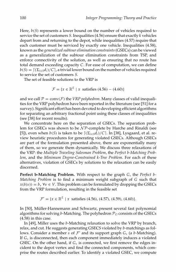
P1: shibuAugust 23, 2005 10:18 1914 1914˙CH04


Here, b(S) represents a lower bound on the number of vehicles required toservice the set of customers S. Inequalities (4.56) ensure that exactly k vehiclesdepart from and returning to the depot, while inequalities (4.57) require thateach customer must be serviced by exactly one vehicle. Inequalities (4.58),known as the generalized subtour elimination constraints (GSECs) can be viewedas a generalization of the subtour elimination constraints from TSP, andenforce connectivity of the solution, as well as ensuring that no route hastotal demand exceeding capacity C . For ease of computation, we can defineb(S) = ( i∈Sdi )/C, a trivial lower bound on the number of vehicles requiredto service the set of customers S.

The set of feasible solutions to the VRP is

F = x ∈ RE | x satisfies (4.56) − (4.60)

and we call P = conv(F) the VRP polyhedron. Many classes of valid inequali-ties for the VRP polyhedron have been reported in the literature (see [51] for asurvey). Significant effort has been devoted to developing efficient algorithmsfor separating an arbitrary fractional point using these classes of inequalities(see [38] for recent results).

We concentrate here on the separation of GSECs. The separation prob-lem for GSECs was shown to be NP-complete by Harche and Rinaldi (see[5]), even when b(S) is taken to be ( i∈Sdi )/C. In [38], Lysgaard, et al. re-view heuristic procedures for generating violated GSECs. Although GSECsare part of the formulation presented above, there are exponentially manyof them, so we generate them dynamically. We discuss three relaxations ofthe VRP: the Multiple Traveling Salesman Problem, the Perfect b-Matching Prob-lem, and the Minimum Degree-Constrained k-Tree Problem. For each of thesealternatives, violation of GSECs by solutions to the relaxation can be easilydiscerned.

Perfect b-Matching Problem. With respect to the graph G, the Perfect b-Matching Problem is to find a minimum weight subgraph of G such thatx(δ(v)) = bv ∀v ∈ V. This problem can be formulated by dropping the GSECsfrom the VRP formulation, resulting in the feasible set

F ′ = x ∈ RE | x satisfies (4.56), (4.57), (4.59), (4.60).

In [50], Muller-Hannemann and Schwartz, present several fast polynomialalgorithms for solving b-Matching. The polyhedronPO consists of the GSECs(4.58) in this case.

In [49], Miller uses the b-Matching relaxation to solve the VRP by branch,relax, and cut. He suggests generating GSECS violated by b-matchings as fol-lows. Consider a member s of F ′ and its support graph Gs (a b-Matching).If Gs is disconnected, then each component immediately induces a violatedGSEC. On the other hand, if Gs is connected, we first remove the edges in-cident to the depot vertex and find the connected components, which com-prise the routes described earlier. To identify a violated GSEC, we compute

P1: shibuAugust 23, 2005 10:18 1914 1914˙CH04


the total demand of each route, checking whether it exceeds capacity. If not,the solution is feasible for the original ILP and does not violate any GSECs.If so, the set S of customers on any route whose total demand exceeds ca-pacity induces a violated GSEC. This separation routine runs in O(|V| +|E |) time and can be used in any of the integrated decomposition meth-ods previously described. Figure 4.20a shows an example vector that couldarise during execution of either price and cut or decompose and cut, alongwith a decomposition into a convex combination of two b-Matchings, shown

0

0

00

0

2

2

2

2

22

2

7

7

7

7

77

7

5

5

5

5

55

5

8

8

8

8

88

8

7

7

7

7

77

7

10

10

10

10

1010

10

4

4

4

4

44

4

0.5

11

11

11

11

0.5

11

11

5

5

0.5

5

5

5

5

11

1

1

1

1

1

1

5

13

13

13

13

1

13

13

5

5

5

5

5

5

13

4

4

4

5

4

4

4

1

1

1

1

1

0.5

1

0.5

1

1

11

1

1

4

2

2

2

0.5

2

2

2

1

1 2

0.5

0.5

(a) x

(b) b -Matching λ1 = 12 (c) b -Matching λ2 = 1

2

(f) k-DCT λ3 = 14

(d) k-DCT λ1 = 14

(e) k-DCT λ2 = 14

(g) k -DCT λ4 = 14

0

FIGURE 4.20Example of a decomposition into b-Matchings and k-DCTs.

P1: shibuAugust 23, 2005 10:18 1914 1914˙CH04


in Figure 4.20b and c. In this example, the capacity C = 35 and by inspectionwe find a violated GSEC in the second b-Matching (c) with S equal to themarked component. This inequality is also violated by the optimal fractionalsolution, since x(δ(S)) = 3.0 < 4.0 = 2b(S).

Minimum Degree-Constrained k-Tree Problem. A k-tree is defined as a span-ning subgraph of G that has |V| + k edges (recall that G has |V| + 1 vertices).A degree-constrained k-tree (k-DCT), as defined by Fisher in [23], is a k-treewith degree 2k at vertex 0. The Minimum k-DCT Problem is that of finding aminimum cost k-DCT, where the cost of a k-DCT is the sum of the costs onthe edges present in the k-DCT. Fisher [23] introduced this relaxation as partof a Lagrangian relaxation-based algorithm for solving the VRP.

The k-DCT polyhedron is obtained by first adding the redundant constraint

x(E) = |V| + k, (4.61)

then deleting the degree constraints (4.57), and finally, relaxing the capacityto C = i∈Sdi . Relaxing the capacity constraints gives b(S) = 1 for all S ⊆ V,and replaces the set of constraints (4.58) with

∑e∈δ(S)

xe ≥ 2, ∀S ⊆ V, |S| > 1. (4.62)

The feasible region of the Minimum k-DCT Problem is then

F ′ = x ∈ RE | x satisfies (4.56), (4.58), (4.59), (4.61).This time, the polyhedron PO is comprised of the constraints (4.57) and theGSECs (4.58). Since the constraints (4.57) can be represented explicitly, wefocus again on generation of violated GSECs. In [62], Wei and Yu give apolynomial algorithm for solving the Minimum k-DCT Problem that runsin O(|V|2 log |V|) time. In [48], Martinhon et al. study the use of the k-DCTrelaxation for the VRP in the context branch, relax, and cut. Again, considerseparating a member s of F ′ from the polyhedron defined by all GSECS. Itis easy to see that for GSECs, an algorithm identical to that described abovecan be applied. Figure 4.20a also shows a vector that could arise during theexecution of either the price and cut or decompose-and-cut algorithms, alongwith a decomposition into a convex combination of four k-DCTs (Figure 4.20dto g). Removing the depot edges, and checking each components demand,we easily identify the violated GSEC in k-DCT (g).

Multiple Traveling Salesman Problem. The Multiple Traveling Salesman Prob-lem (k-TSP) is an uncapacitated version of the VRP obtained by adding thedegree constraints to the k-DCT polyhedron. The feasible region of the k-TSPis

F ′ = x ∈ RE | x satisfies (4.56), (4.57), (4.59), (4.60), (4.62).Although the k-TSP is an N P-hard optimization problem, small instancescan be solved effectively by transformation into an equivalent TSP obtained

P1: shibuAugust 23, 2005 10:18 1914 1914˙CH04


by adjoining to the graph k − 1 additional copies of vertex 0 and its incidentedges. In this case, the polyhedronPO is again comprised solely of the GSECs(4.58). In [57], Ralphs et al. report on an implementation of branch, decomposeand cut using the k-TSP as a relaxation.

4.8.2 Three-Index Assignment Problem

The Three-Index Assignment Problem (3AP) is that of finding a minimum-weightclique cover of the complete tri-partite graph Kn,n,n. Let I, J, and K be threedisjoint sets with |I | = |J | = |K | = n and set H = I × J × K . 3AP can beformulated as the following binary integer program:

min∑

(i, j,k)∈H

ci jk xi jk ,

∑( j,k)∈J ×K

xi jk = 1 ∀ i ∈ I, (4.63)

∑(i,k)∈I×K

xi jk = 1 ∀ j ∈ J , (4.64)

∑(i, j)∈I×J

xi jk = 1 ∀ k ∈ K, (4.65)

xi jk ∈ 0, 1 ∀ (i, j, k) ∈ H. (4.66)

A number of applications of 3AP can be found in the literature (see Piersjalla[18,19]). 3AP is known to be N P-hard [26]. As before, the set of feasiblesolutions to 3AP is noted as

F = x ∈ RH | x satisfies (4.63) − (4.66)

and we set P = conv(F).In [7], Balas and Saltzman study the polyhedral structure ofP and introduce

several classes of facet-inducing inequalities. Let u, v ∈ H and define |u ∩ v|to be the numbers of coordinates for which the vectors u and v have the samevalue. Let C(u) = w ∈ H | |u ∩ w| = 2 and C(u, v) = w ∈ H | |u ∩ w| =1, |w ∩ v| = 2. We consider two classes of facet-inducing inequalities Q1(u)

and P1(u, v) for P ,

xu +∑

w∈C(u)

xw ≤ 1 ∀ u ∈ H, (4.67)

xu +∑

w∈C(u,v)

xw ≤ 1 ∀ u, v ∈ H, |u ∩ v| = 0. (4.68)

Note that these include all the clique facets of the intersection graph of Kn,n,n

[7]. In [6], Balas and Qi describe algorithms that solve the separation problemfor the polyhedra defined by the inequalities Q1(u) and P1(u, v) in O(n3)

time.

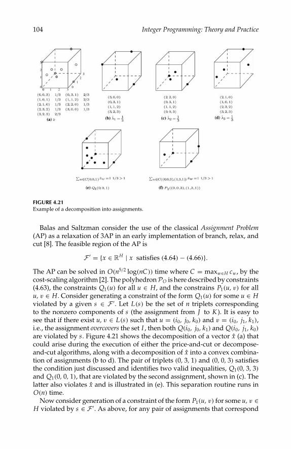
P1: shibuAugust 23, 2005 10:18 1914 1914˙CH04


FIGURE 4.21Example of a decomposition into assignments.

Balas and Saltzman consider the use of the classical Assignment Problem(AP) as a relaxation of 3AP in an early implementation of branch, relax, andcut [8]. The feasible region of the AP is

F ′ = x ∈ RH | x satisfies (4.64) − (4.66).The AP can be solved in O(n5/2 log(nC)) time where C = maxw∈H cw, by thecost-scaling algorithm [2]. The polyhedronPO is here described by constraints(4.63), the constraints Q1(u) for all u ∈ H, and the constrains P1(u, v) for allu, v ∈ H. Consider generating a constraint of the form Q1(u) for some u ∈ Hviolated by a given s ∈ F ′. Let L(s) be the set of n triplets correspondingto the nonzero components of s (the assignment from J to K ). It is easy tosee that if there exist u, v ∈ L(s) such that u = (i0, j0, k0) and v = (i0, j1, k1),i.e., the assignment overcovers the set I , then both Q(i0, j0, k1) and Q(i0, j1, k0)

are violated by s. Figure 4.21 shows the decomposition of a vector x (a) thatcould arise during the execution of either the price-and-cut or decompose-and-cut algorithms, along with a decomposition of x into a convex combina-tion of assignments (b to d). The pair of triplets (0, 3, 1) and (0, 0, 3) satisfiesthe condition just discussed and identifies two valid inequalities, Q1(0, 3, 3)

and Q1(0, 0, 1), that are violated by the second assignment, shown in (c). Thelatter also violates x and is illustrated in (e). This separation routine runs inO(n) time.

Now consider generation of a constraint of the form P1(u, v) for some u, v ∈H violated by s ∈ F ′. As above, for any pair of assignments that correspond

P1: shibuAugust 23, 2005 10:18 1914 1914˙CH04


to nonzero components of s and have the form (i0, j0, k0), (i0, j1, k1), we knows violates P1((i0, j0, k0), (i, j1, k1)), ∀i = i0 and P1((i0, j1, k1), (i, j0, k0)), ∀i =i0. The inequality P1((0, 0, 3), (1, 3, 1)) is violated by the second assignment,shown in Figure 4.21(c). This inequality is also violated by x and is illustratedin (f). Once again, this separation routine runs in O(n) time.

4.8.3 Steiner Tree Problem

Let G = (V, E) be a complete undirected graph with vertex set V = 1, . . . ,|V|, edge set E and a positive weight ce associated with each edge e ∈ E .Let T ⊂ V define the set of terminals. The Steiner Tree Problem (STP), whichis N P-hard, is that of finding a subgraph that spans T (called a Steiner tree)and has minimum edge cost. In [13], Beasley formulated the STP as a sideconstrained Minimum Spanning Tree Problem (MSTP) as follows. Let r ∈ T besome terminal and define an artificial vertex 0. Now, construct the augmentedgraph G = (V, E) where V = V ∪ 0 and E = E ∪ i, 0 | i ∈ (V \ T) ∪ r.Let ci0 = 0 for all i ∈ (V \ T) ∪ r. Then, the STP is equivalent to finding aminimum spanning tree (MST) in G subject to the additional restriction thatany vertex i ∈ (V \ T) connected by edge i, 0 ∈ E must have degree one.

By associating a binary variable xe with each edge e ∈ E , indicating whetheror not the edge is selected, we can then formulate the STP as the followinginteger program:

min∑e∈E

ce xe ,

x(E) = |V| − 1, (4.69)x(E(S)) ≤ |S| − 1 ∀S ⊆ V, (4.70)xi0 + xe ≤ 1 ∀e ∈ δ(i), i ∈ (V \ T), (4.71)

xe ∈ 0, 1 ∀e ∈ E . (4.72)

Inequalities (4.69) and (4.70) ensure that the solution forms a spanning treeon G. Inequalities (4.70) are subtour elimination constraints (similar to thoseused in the TSP). Inequalities (4.71) are the side constraints that ensure thesolution can be converted to a Steiner tree by dropping the edges in E \ E .

The set of feasible solutions to the STP is

F = x ∈ RE | x satisfies (4.69) − (4.72).We set P = conv(F) as before. We consider two classes of valid inequalitiesfor P that are lifted versions of the subtour elimination constraints (SEC).

x(E(S)) + x(E(S \ T | 0)) ≤ |S| − 1 ∀S ⊆ V, S ∩ T = ∅, (4.73)x(E(S)) + x(E(S \ v | 0)) ≤ |S| − 1 ∀S ⊆ V, S ∩ T = ∅, v ∈ S. (4.74)

The class of valid inequalities (4.73) were independently introduced byGoemans [27], Lucena [44] and Margot, Prodon, and Liebling [47], for another

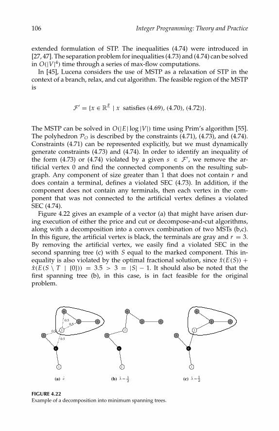
P1: shibuAugust 23, 2005 10:18 1914 1914˙CH04


extended formulation of STP. The inequalities (4.74) were introduced in[27, 47]. The separation problem for inequalities (4.73) and (4.74) can be solvedin O(|V|4) time through a series of max-flow computations.

In [45], Lucena considers the use of MSTP as a relaxation of STP in thecontext of a branch, relax, and cut algorithm. The feasible region of the MSTPis

F ′ = x ∈ RE | x satisfies (4.69), (4.70), (4.72).

The MSTP can be solved in O(|E | log |V|) time using Prim’s algorithm [55].The polyhedron PO is described by the constraints (4.71), (4.73), and (4.74).Constraints (4.71) can be represented explicitly, but we must dynamicallygenerate constraints (4.73) and (4.74). In order to identify an inequality ofthe form (4.73) or (4.74) violated by a given s ∈ F ′, we remove the ar-tificial vertex 0 and find the connected components on the resulting sub-graph. Any component of size greater than 1 that does not contain r anddoes contain a terminal, defines a violated SEC (4.73). In addition, if thecomponent does not contain any terminals, then each vertex in the com-ponent that was not connected to the artificial vertex defines a violatedSEC (4.74).

Figure 4.22 gives an example of a vector (a) that might have arisen dur-ing execution of either the price and cut or decompose-and-cut algorithms,along with a decomposition into a convex combination of two MSTs (b,c).In this figure, the artificial vertex is black, the terminals are gray and r = 3.By removing the artificial vertex, we easily find a violated SEC in thesecond spanning tree (c) with S equal to the marked component. This in-equality is also violated by the optimal fractional solution, since x(E(S)) +x(E(S \ T | 0)) = 3.5 > 3 = |S| − 1. It should also be noted that thefirst spanning tree (b), in this case, is in fact feasible for the originalproblem.

1 1 1

2 2 2

3 3 3

0.5

4440.5

5 55

6 6

6

6

6

0.5

6

0.5

(a) x (b) λ = 12

12(c) λ =

FIGURE 4.22Example of a decomposition into minimum spanning trees.

P1: shibuAugust 23, 2005 10:18 1914 1914˙CH04


4.9 Conclusions and Future Work

In this chapter, we presented a framework for integrating dynamic cut genera-tion (outer methods) and traditional decomposition methods (inner methods)to yield new integrated methods that may produce bounds that are improvedover those yielded by either technique alone. We showed the relationshipsbetween the various methods and how they can be viewed in terms of polyhe-dral intersection. We have also introduced the concept of structured separa-tion and a related paradigm for the generation of improving inequalities basedon decomposition and the separation of solutions to a relaxation. The nextstep in this research is to complete a computational study using the softwareframework introduced in Section 4.7 that will allow practitioners to makeintelligent choices between the many possible variants we have discussed.

References

1. Aardal, K. and van Hoesel, S., Polyhedral techniques in combinatorial opti-mization, Statistica Neerlandica, 50, 3, 1996.

2. Ahuja, R., Magnanti, T., and Orlin, J., Network Flows: Theory, Algorithms, andApplications, Prentice Hall, Englewood Cliffs, NJ, 1993.

3. Applegate, D., Bixby, R., Chvatal, V., and Cook, W., TSP cuts which do notconform to the template paradigm, in Computational Combinatorial Optimization,pages 261–303, Springer, 2001.

4. Applegate, D., Bixby, R., Chvatal, V., and Cook, W., Implementing the Dantzig-Fulkerson-Johnson algorithm for large traveling salesman problems, Mathe-matical Programming, 97, 91, 2003.

5. Augerat, P. et al., Computational Results with a Branch and Cut Code forthe Capacitated Vehicle Routing Problem, Technical Report 949-M, UniversiteJoseph Fourier, Grenoble, France, 1995.

6. Balas, E. and Qi, L., Linear-time separation algorithms for the three-index as-signment polytope, Discrete Applied Mathematics, 43, 1, 1993.

7. Balas, E. and Saltzman, M., Facets of the three-index assignment polytope,Discrete Applied Mathematics, 23, 201, 1989.

8. Balas, E. and Saltzman, M., An algorithm for the three-index assignment prob-lem, Operations Research, 39, 150, 1991.

9. Barahona, F. and Anbil, R., The volume algorithm: Producing primal solutionswith a subgradient method, Mathematical Programming, 87, 385, 2000.

10. Barahona, F. and Jensen, D., Plant location with minimum inventory, Mathe-matical Programming, 83, 101, 1998.

11. Barnhart, C., Hane, C. A., and Vance, P. H., Using branch-and-price-and-cutto solve origin-destination integer multi-commodity flow problems, OperationsResearch, 48, 318, 2000.

12. Barnhart, C., Johnson, E. L., Nemhauser, G. L., Savelsbergh, M. W. P., and Vance,P. H., Branch and price: Column generation for solving huge integer programs,Operations Research, 46, 316, 1998.

P1: shibuAugust 23, 2005 10:18 1914 1914˙CH04


13. Beasley, J., A SST-based algorithm for the steiner problem in graphs, Networks,19, 1, 1989.

14. Beasley, J., Lagrangean relaxation, in Modern Heuristic Techniques for Combinato-rial Optimization, edited by Reeves, C., Wiley, 1993.

15. Belloni, A. and Lucena, A., A Lagrangian heuristic for the linear ordering prob-lem, in Metaheuristics: Computer Decision-Making, edited by Resende, M. andde Sousa, J. P., pages 123–151, Kluwer Academic, 2003.

16. Calheiros, F. C., Lucena, A., and de Souza, C., Optimal rectangular partitions,Networks, 41, 51, 2003.

17. Caprara, A., Fischetti, M., and Toth, P., Algorithms for the set covering problem,Annals of Operations Research, 98, 353, 2000.

18. Carraresi, P., Frangioni, A., and Nonato, M., Applying bundle methods to opti-mization of polyhedral functions: An applications-oriented development, Tech-nical Report TR-96-17, Universita di Pisa, 1996.

19. Dantzig, G. and Wolfe, P., Decomposition principle for linear programs, Opera-tions Research, 8, 101, 1960.

20. Danzig, G. and Ramser, R., The truck dispatching problem, Management Sci-ence, 6, 80, 1959.

21. de Aragao, M. P. and Uchoa, E., Integer program reformulation for robustbranch-and-cut-and-price, Working paper, Pontifica Universidade Catolica doRio de Janeiro, 2004, Available from http://www.inf.puc-rio.br/˜uchoa/doc/rbcp-a.pdf.

22. Fisher, M., The Lagrangian relaxation method for solving integer programmingproblems, Management Science, 27, 1, 1981.

23. Fisher, M., Optimal solution of vehicle routing problems using minimum k-trees, Operations Research, 42, 626, 1994.

24. Fukasawa, R., de Aragao, M. P., Reis, M., and Uchoa, E., Robust branch-and-cut-and-price for the capacitated minimum spanning tree problem, in Proceedingsof the International Network Optimization Conference, pages 231–236, Evry, France,2003.

25. Galati, M., DECOMP user’s manual, Technical report, Lehigh University In-dustrial and Systems Engineering, 2005.

26. Garey, M. R. and Johnson, D. S., Computers and Intractability: A Guide to the Theoryof NP-Completeness, W. H. Freeman and Company, New York, 1979.

27. Goemans, M., The steiner tree polytope and related polyhedra, MathematicalProgramming, 63, 157, 1994.

28. Goffin, J. L. and Vial, J. P., Convex nondifferentiable optimization: A surveyfocused on the analytic center cutting plane method, Technical Report 99.02,Logilab, Geneva, Switzerland, 1999.

29. Gondzio, J. and Sarkissian, R., Column generation with a primal-dual method,Technical report, University of Geneva, Logilab, HEC Geneva, 1996.

30. Grotschel, M. and Padberg, M., On the symmetric travelling salesman problemI: Inequalities, Mathematical Programming, 16, 265, 1979.

31. Grotschel, M. and Padberg, M., On the symmetric travelling salesman problemII: Lifting theorems and facets, Mathematical Programming, 16, 281, 1979.

32. Grotschel, M. and Lovasz, L. and Schrijver, A., The ellipsoid method and itsconsequences in combinatorial optimization, Combinatorica, 1, 169, 1981.

33. Guignard, M., Efficient cuts in Lagrangean “relax-and-cut” schemes, EuropeanJournal of Operational Research, 105, 216, 1998.

34. Guignard, M., Lagrangean relaxation, Top, 11, 151, 2003.

P1: shibuAugust 23, 2005 10:18 1914 1914˙CH04


35. Held, M. and Karp, R. M., The traveling salesman problem and minimumspanning trees, Operations Research, 18, 1138, 1970.

36. Huisman, D., Jans, R., Peeters, M., and Wagelmans, A., Combining column gen-eration and Lagrangian relaxation, Technical report, Erasmus Research Instituteof Management, Rotterdamn, The Netherlands, 2003.

37. Hunting, M., Faigle, U., and Kern, W., A Lagrangian relaxation approach tothe edge-weighted clique problem, European Journal of Operational Research, 131,119, 2001.

38. J. Lysgaard, A. L. and Eglese, R., A new branch-and-cut algorithm for the ca-pacitated vehicle routing problem, Mathematical Programming, 100, 423, 2004.

39. Kohl, N., Desrosiers, J., Madsen, O., Solomon, M., and Soumis, F., 2-path cutsfor the vehicle routing problem with time windows, Transportation Science, 33,101, 1999.

40. Kopman, L., A New Generic Separation Routine and Its Application In a Branchand Cut Algorithm for the Capacitated Vehicle Routing Problem, PhD thesis, CornellUniversity, 1999.

41. Laporte, G., Nobert, Y., and Desrouchers, M., Optimal routing with capacityand distance restrictions, Operations Research, 33, 1050, 1985.

42. Linderoth, J. and Galati, M., Knapsack constrained circuit problem, Unpub-lished working paper, 2004.

43. Lubbecke, M. E. and Desrosiers, J., Selected topics in column generation, Tech-nical Report 008-2004, Technische Universitat Berlin, 2004.

44. Lucena, A., Tight bounds for the Steiner problem in graphs, Talk given atTIMS-XXX-SOBRAPO XXIII Joint International Meeting, Rio de Janeiro, 1991.

45. Lucena, A., Steiner problem in graphs: Lagrangian relaxation and cuttingplanes, COAL Bulletin, 28, 2, 1992.

46. Lucena, A., Nondelayed relax-and-cut algorithms, Working paper, Depart-maneto de Administrac ao, Universidade Federal do Rio de Janeiro, 2004.

47. Margot, F., Prodon, A., and Liebling, T., Tree polyhedron on 2-tree, MathematicalProgramming, 63, 183, 1994.

48. Martinhon, C., Lucena, A., and Maculan, N., Stronger k-tree relaxations forthe vehicle routing problem, European Journal of Operational Research, 158, 56,2004.

49. Miller, D., A matching based exact algorithm for capacitated vehicle routingproblems, ORSA Journal on Computing, 7, 1, 1995.

50. Muller-Hannemann, M. and Schwartz, A., Implementing weighted b-matchingalgorithms: Toward a flexible software design, in Proceedings of the Workshop onAlgorithm Engineering and Experimentation (ALENEX99), volume 1619 of Lecturenotes in Computer Science, pages 18–36, Baltimore, MD, 1999, Springer-Verlag.

51. Naddef, D. and Rinaldi, G., Branch-and-cut algorithms for the capacitated VRP,in The Vehicle Routing Problem, edited by Toth, P. and Vigo, D., pages 53–84, SIAM,2002.

52. Nemhauser, G. and Wolsey, L., Integer and Combinatorial Optimization, Wiley,New York, 1988.

53. Padberg, M. and Rinaldi, G., An efficient algorithm for the minimum capacitycut problem, Mathematical Programming, 47, 19, 1990.

54. Pigatti, A., Modelos e algoritmos para o problema de alocao generalizada e aplicacoes,PhD thesis, Pontificia Universidade Catolica do Rio de Janeiro, 2003.

55. Prim, R., Shortest connection networks and some generalizations, Bell SystemTechnical Journal, 36, 1389, 1957.

P1: shibuAugust 23, 2005 10:18 1914 1914˙CH04


56. Ralphs, T., Parallel Branch and Cut for Vehicle Routing, PhD thesis, Cornell Uni-versity, 1995.

57. Ralphs, T., Kopman, L., Pulleyblank, W., and Trotter Jr., L., On the capacitatedvehicle routing problem, Mathematical Programming, 94, 343, 2003.

58. Rousseau, L. M., Gendreau, M., and Feillet, D., Interior point stabilization forcolumn generation, Working paper, Cahier du Gerad, 2003, Available fromhttp://www.lia.univ-avignon.fr/fich_art/380-IPS.pdf.

59. V. Chvatal, Linear Programming, W.H. Freeman and Company, 1983.60. van den Akker, J., Hurkens, C., and Savelsbergh, M., Time-indexed formulations

for machine scheduling problems: Column generation, INFORMS Journal onComputing, 12, 111, 2000.

61. Vanderbeck, F., Lot-sizing with start-up times, Management Science, 44, 1409,1998.

62. Wei, G. and Yu, G., An improved O(n2 log n) algorithm for the degree-constrained minimum k-tree problem, Technical report, The University of Texasat Austin, Center for Management of Operations and Logistics, 1995.

P1: shibu/Vijay

August 12, 2005 10:24 1914 1914˙C005

5Airline Scheduling Models and SolutionAlgorithms for the Temporary Closureof Airports

Shangyao Yan and Chung-Gee Lin

CONTENTS

5.1 Introduction . . . . . . . . . . . . . . . . . . . . . . . . . . . . . . . 1115.2 The Basic Model . . . . . . . . . . . . . . . . . . . . . . . . . . . . . 1145.3 The Strategic Models . . . . . . . . . . . . . . . . . . . . . . . . . . 119

5.3.1 Rule (a) The Swap of Aircraft Types . . . . . . . . . . . . . 1195.3.2 Rule (b) Flight Delays . . . . . . . . . . . . . . . . . . . . . 1205.3.3 Rule (c) Modification of Multi-Stop Flights . . . . . . . . . 1225.3.4 Rule (d) Ferrying of Idle Aircraft . . . . . . . . . . . . . . . 123

5.4 Solution Methods . . . . . . . . . . . . . . . . . . . . . . . . . . . . 1245.5 Case Study . . . . . . . . . . . . . . . . . . . . . . . . . . . . . . . . 1265.6 Conclusions . . . . . . . . . . . . . . . . . . . . . . . . . . . . . . . 132Acknowledgments . . . . . . . . . . . . . . . . . . . . . . . . . . . . . . 134References . . . . . . . . . . . . . . . . . . . . . . . . . . . . . . . . . . . 134

5.1 Introduction

The temporary closure of airports usually results in significant perturbationsof flight schedules. For example, typhoons or periods of heavy rain hap-pen from time to time in Taiwan each year. The airports usually have to betemporarily closed, and many flights are then canceled or delayed. The poorscheduling of flights, or an entire fleet, may result in a substantial loss of profitand decreased levels of service for airline carriers. Thus, effective and efficientflight/fleet incident management is important for carriers in order to regaintheir normal services as soon as possible following a schedule perturbation.

The current process for handling the schedule perturbations from a tempo-rary closure of airports for the carriers in Taiwan is inefficient and ineffectivefrom a system perspective, especially for large flight networks. The typicalprocess is as follows. When an airport is closed temporarily, a scheduling

111

P1: shibu/Vijay

August 12, 2005 10:24 1914 1914˙C005


group in the System Operations Control department (SOC) starts by choos-ing a suitable strategy, the expected time for the airport to open, the regularplanned schedule, projected (with booked) demand on all flights and the allo-cation of the currently available airplanes. The detailed flight/fleet scheduleis then adjusted by a trial-and-error process until a feasible solution is found.For example, if a flight cannot be served because the airport is closed, thenit may be delayed until the airport is reopened, or it may be canceled if itis delayed too long. For another example, if a flight cannot be served by itsscheduled aircraft (probably due to the closure of an upstream airport), thenthe flight may be suitably delayed so that a holding aircraft (or an incom-ing aircraft) can be rescheduled to serve this flight; however, if there is noholding aircraft (or no incoming aircraft), then the flight may be canceled, orserved by an aircraft obtained from another station using a ferry flight. Sucha process generally involves a series of local adjustments (usually by hand)of the aircraft routes and related flights. When the network size grows, thisprocess becomes inefficient for finding the optimal solution. Typically, onlya feasible solution is obtained under the real time constraint. The draftedschedule is then shuttled to other groups in the SOC for the application ofother constraints (for example crew constraints or maintenance constraints).The schedule will be executed if proves feasible; otherwise, it will be returnedto the scheduling group for schedule revisions. The process is repeated untilall groups are satisfied with the revised schedule.

Due to deregulation, the flight networks for carriers in Taiwan have recentlygrown. In particular, to enhance operations, carriers have been purchasing dif-ferent types of aircraft suitable for different flight mileages to form multi-fleetoperations, in order to improve their profit. If the schedule is perturbed fol-lowing accidents, in a multi-fleet operation airplanes of different types cansupport each other through new routing with a temporary flight schedule.For example; a) some idle larger-sized aircraft can serve flights scheduledfor smaller-sized aircraft, b) some idle smaller-sized aircraft can serve flightsscheduled for larger-sized aircraft, if passengers not able to board the smaller-sized aircraft are allowed to cancel, or can be reaccommodated on suitableflights or alternate modes to the same destinations. For another example,some flights could be delayed so that other-sized aircraft can be resched-uled to serve these flights if this is profitable from the system aspect. Since asingle-fleet scheduling model may not be adequate to evaluate such sched-ule perturbations, it would be helpful for carriers to have multi-fleet modelsto handle schedule perturbations both efficiently and effectively and thus toreduce losses resulting from airport closures.

As a result of growing size of fleet, it is increasingly difficult for the tradi-tional approach to adequately handle schedule incidents. It would be helpfulfor carriers to have systematic computerized models to handle schedule per-turbations efficiently and effectively, so as to reduce losses resulting fromairport closures. The past studies on airline schedule perturbations can typi-cally be classified into two topics: one, the shortage of aircraft and the other,the closure of airports (Yan and Lin [22]).

P1: shibu/Vijay

August 12, 2005 10:24 1914 1914˙C005

Airline Scheduling Models and Solution Algorithms 113

For schedule perturbations on aircraft shortages, relatively more researchhas been done. In particular, Deckwitz [5] introduced “positioning flights”and “sliding flights”. The former denotes a relocation of some reserved air-planes to serve certain flights. The latter indicates the delay of a flight’s depar-ture time within a slot time to better adjust that flight’s connections. Jedlin-sky [11] applied a minimum cost network flow problem to solve scheduleperturbation using the out-of-kilter algorithm. Etschmaier and Rothstein [6]built a simulation model for evaluating flight punctuality. Teodorovic andGuberinic [17] developed a nonlinear integer model by setting the objectiveto be a minimization of the total passenger delay. Gershkoff [9] used a time-space framework to formulate fleet routing and applied a successive shortestpath method to find arc chains for the cancellation of a series of flights becauseof a shortage of aircraft. Teodorovic and Stojkovic [18] developed a greedyheuristic for solving a goal programming problem. Given some perturbationsin the flight schedule, the heuristic finds the new set of aircraft routings thatfirst minimizes the number of cancellations, and then minimizes the overallpassenger delays. Jarrah et al. [10] proposed two minimum cost network flowmodels to systematically adjust aircraft routing and flight scheduling in realtime, to minimize the total cost incurred from a shortage of aircraft. The “delaymodel” applied flight delays and aircraft swaps at a station, and the “cancel-lation model” applied flight cancellations and aircraft swaps among stationsto handle aircraft routing and flight scheduling. Yan and Yang [24] have in-corporated flight cancellations, delays and ferry flights into four time-spacenetwork models in order to resolve schedule recovery problems arising from atemporary shortage of aircraft, for single-fleet and nonstop flight operations.Yan and Tu [23] have extended Yan and Yang’s models to multiple-fleet andmultiple-stop flight operations. Thengvall et al. [19] have extended the workof Yan et al. [22–24] to the building of recovery schedules by the inclusionof an incentive in the formulation that will minimize any deviation from theoriginal aircraft routings.

For schedule perturbations on airport closures, Jedlinsky [11] has intro-duced a network using the local modification of links to handle schedule per-turbations resulting from the closure of an airport. The modified network wasformulated as a minimum cost network flow problem which was solved usingthe out-of-kilter algorithm. Teodorovic [15] has developed a model for design-ing the most meteorologically reliable airline schedule, which however, wasnot focused on schedule perturbations to execute a planned airline schedule.Yan and Lin [22] have used time-space networks to develop eight schedulingmodels for single-fleet and multiple-stop operations dealing with the tempo-rary closure of airports. Thengvall et al. [20] have incorporated flight cancel-lations, delays, ferry flights and substitutions between fleets and sub-fleets, toformulate three multi-commodity network models for the large carriers thathave to deal with a hub closure. Compared to the aircraft shortage literature,not much research has been done on schedule perturbations resulting fromthe temporary closure of airports. Moreover, most of the former research onairline schedule perturbations was focused on the operations of a single fleet.

P1: shibu/Vijay

August 12, 2005 10:24 1914 1914˙C005


To improve the traditional scheduling process, this research modifies the pro-cess by solving the scheduling problem using several strategic models whichcombine the traditional scheduling rules in a systematic scheme.

This research aims to develop a set of models to help carriers handle sched-ule perturbations resulting from the temporary closure of airports. A basicmodel is first constructed as a multiple time-space network, from which sev-eral perturbed network models are developed for rescheduling followingincidents. The scope of this research is confined to the operations of a mul-tiple fleet as well as one-stop and nonstop flights. The operations involvedin other types of multi-stop flights and the schedule perturbation caused byother types of incidents are left to be addressed in the future. In addition, thisresearch focuses on a case where an airport is temporarily closed. Althoughthe model developed in this research needs to be modified to handle caseswhere more than one airport is closed at the same time, we believe modifica-tion to be easy, a subject also left for future research.

Although there is a significant interdependence between the airline sched-ule design process and aircraft maintenance, as well as the crew schedulingprocesses, these processes are usually separated in order to facilitate prob-lem solving (Teodorovic, [16]). This research thus excludes the constraints ofaircraft maintenance and crew scheduling in the modeling. In practice, thefleet routes and flight schedules obtained from these models can serve as agood initial solution for the minor modification of these constraints. How-ever, actually incorporating these constraints into a complicated frameworkwould be a topic for future research.

The rest of this chapter is organized as follows: first, we formulate our mod-els, including a basic model and several strategic models. These models areformulated as integer programs and their solutions are developed hereafter.A case study is then performed to test the models in the real world. Finally,we offer conclusions.

5.2 The Basic Model

In practice, most carriers’ primary objective for adjusting schedule perturba-tion following incidents is to resume their normal services as soon as possiblein order to maintain their levels of service. Given the time length of a scheduleperturbation, carriers typically aim to adjust a schedule to minimize the lossof system profit. Thus, the basic model is designed to minimize the schedule-perturbed period after an incident and to obtain the most profitable schedulegiven the schedule-perturbed period.

The basic model contains several fleet networks, each formulating a singlefleet operation in the schedule-perturbed period. This research suggests usinga time-space network, as shown in Figure 5.1, to formulate a single fleetoperation in the basic mode, because it is natural to represent conveyanceroutings in the dimensions of time and space (see, for example, Yan et al. [21]).

P1: shibu/Vijay

August 12, 2005 10:24 1914 1914˙C005


(2) (1)

the ending time

the recovery time

the starting time

(4) (4) (4)

(3)(5)

(7)

(8)

kCity City 3 (closed)City 2City 1

(6)

(6)

(4) final demand (3) intermediate demand (2) intermediate supply (1) initial supply

(4)

(5) position arc(6) flight arc(7) ground arc(8) overnight arc

FIGURE 5.1The single-fleet basic model.

To develop strategic models based on the basic model, only a few nodes,links, or additional side constraints need to be modified, without changingthe original network structure. In Figure 5.1, the horizontal axis representsairport locations, while the vertical axis represents the time duration. Eachnode represents a specific airport at a specific time. Each arc represents anactivity for an airplane. There are four types of arcs described below:

Flight arc: representing a nonstop flight or a one-stop flight. The time win-dow for a nonstop flight is calculated as a block of time, from the time whenan airplane begins to prepare for this flight to the time when the airplane fin-ishes the flight and is ready for the next flight service or holding. If the flightis a multiple-stop flight, then the time block is from the beginning of the firstleg to the end of the last leg. The time block includes the time for investi-gating aircraft before departure, fueling, passenger/baggage boarding anddeplaning, and flight time in the air. The arc cost equals the flight cost minus

P1: shibu/Vijay

August 12, 2005 10:24 1914 1914˙C005


passenger revenues. The arc flow upper bound is one, meaning that at mostone airplane can serve this flight. The arc flow lower bound is zero, indicatingthat this flight can be canceled. Additional charges for canceling flights can beincurred; for example, to reaccommodate the passengers of canceled flightson suitable flights or alternate modes to the same destinations. To reflect suchcharges, we set the cost function for a flight from i to j as Ccn

ij + Cdnij

∗ Xnij, where

Xnij is the flow on arc (i, j) in the nth fleet network, which is equal to zero or one,

Ccnij is the cancellation cost and Cdn

ij equals the flight arc cost minus the can-cellation cost, Cn

ij − Ccnij. Therefore, if the flight (i, j) is served (that is, Xn

ij = 1),then the cost is Cn

ij; otherwise (that is, Xnij = 0), the cost is Ccn

ij. Note that forflight arcs connected to the closed airport within the unavailable period, theirupper bounds are set as zero, meaning that these flights are canceled unlessother strategies are applied to modify the flights to be served.

Ground arc: representing the holding of airplanes at an airport in a timewindow. The time window lies between two adjacent flight event times(landing/taking-off) at an airport. The arc cost represents the expenses in-curred by holding an airplane at the airport in the time window, includingthe airport tax, airport holding charges and gate use charges. The arc flowupper bound is equal to the apron capacity, representing the greatest numberof airplanes that can be held at this airport during this time window. The arcflow lower bound is zero, meaning that a minimum of zero airplanes are heldat this airport in this time window.

Overnight arc: representing the holding of airplanes overnight at an airport.The time window is set for the overnight duration between two consecutivedays. The arc cost is the cost for an airplane held overnight, which is similar tothat of a ground arc with an additional overnight charge. The arc flow upperbound and lower bound are set to be the same as those of the ground arcs.

Position arc: representing a ferry flight between two airports. This is similarto a flight arc; except that the arc cost excludes passenger revenue, and theblock time excludes passenger boarding/deplaning time and package han-dling time, and the arc flow upper bound is equal to the airport departurecapacity.

The network contains a perturbed period from a starting time to an endingtime. The recovery time indicates the time that the closed airport is opened.The starting time is when an airport is closed. At the starting time all airplaneslocated at airports or in the air, are set as initial or intermediate node supplies.The ending time is when the fleet resumes its normal operations. The endingtime is determined as follows. In order to ensure a feasible solution in thedesigned network and to minimize the perturbed period, position arcs areadded from the nodes when the closed airport is opened. Through theseposition arcs, the airplanes can be at least relocated to suitable airports byferry flights. Thus the fleet can resume its regular service. In order to ensurethat all airplanes are relocated in time to the destination of such ferry flights,we set the ending time to be the latter of the following two times: the last

P1: shibu/Vijay

August 12, 2005 10:24 1914 1914˙C005


arrival time of all the position arcs and the last arrival time of flights whichdepart earlier than the times their corresponding ferry flights arrive. Final orintermediate node demands are set according to the normal fleet allocationat airports, or in the air, at the ending time. Note that if more than one airportis closed at the same time, the ending time can be set using the same method,except it is the last one calculated among them all. This research however,assumes only one closed airport at a time for simplification. It should alsobe noted that the airport authority might possibly update estimates of anairport’s opening time. For this reason, the models should be dynamicallyapplied. In particular, a new network should be updated in such a case, anew starting time and a new ending time. After solving the new network, theschedule should be revised again.

To formulate the basic model involving multi-fleet operations, we use amultiple time-space network (as shown in Figure 5.2) assuming there arethree fleets in the operation. Each fleet network in Figure 5.2 is designed thesame as that in Figure 5.1. Note that the ending time of the system is the lastending time calculated in each fleet network.

The integer program formulating the basic model is shown below:

Min Z =∑n∈M

∑

i, j∈An\F n

Cnij Xn

ij +∑

i, j∈F n

Cndij

Xnij

+∑

i, j∈F n

Cncij

(5.1)

s.t.∑

j∈On(i)

Xnij

−∑

k∈I n(i)

Xnki

= bni, ∀i ∈ N,∀n ∈ M (5.2)

0 ≤ Xnij

≤ Unij

, ∀(i, j) ∈ A, ∀n ∈ M (5.3)

Xnij ∈ I, ∀(i, j) ∈ A, ∀n ∈ M (5.4)

where:n : the nth fleetM : the set of all fleetsNn : the set of all nodes in the nth fleet networkAn : the set of all arcs in the nth fleet networkF n : the set of all flight arcs in the nth fleet networkOn(i) : the set of head nodes for arcs emanating from node i in the

nth fleet networkI n(i) : the set of tail nodes for arcs pointing into node i in the

nth fleet networkbn

i : the node supply/demand of node i in the nth fleet networkCn

ij , Xnij , Un

ij : arc (i, j) cost, flow and flow upper bound, respectively in thenth fleet network

Cncij : the cancellation cost for flight (i, j) in the nth fleet network

Cndij : equal to Cn

ij − Cncij

The objective of this model is to “flow” all node supplies to all node de-mands in each network at a minimum cost. Since passenger revenues areformulated as negative costs, the objective is equivalent to a maximization of

P1: shibu/Vijay

August 12, 2005 10:24 1914 1914˙C005


a1

a2

b1

b2

b3

c1

c2

a1, a2: type A flight arcsb1, b2, b3: type B flight arcsc1, c2: type C flight arcs

the starting time

the recovery time

the ending time

1 2 3 k 1 2 3 k 1 2 3 k

FIGURE 5.2The multi-fleet basic model.

the total system profit. Constraint (5.1) is the flow conservation constraint, atevery node, in each fleet network. Constraint (5.2) ensures that all arc flowsare within their upper and lower bounds in each fleet network, and constraint(5.3) ensures that all arc flows are integers in each fleet network. Note that thebasic model can be used to evaluate the cancellation of flights. When n = 1,the integer program formulates a single-fleet scheduling model. As n ≥ 2,the integer program describes a multi-fleet scheduling model. Since any fleetnetwork is independent of the other fleet networks, the basic model can becharacterized as a single-fleet scheduling model.

P1: shibu/Vijay

August 12, 2005 10:24 1914 1914˙C005


5.3 The Strategic Models

To make the basic model more useful, four practical scheduling rules are in-corporated to develop strategic models, in particular, (a) the swap of aircrafttypes (b) flight delays, (c) the modification of one-stop flights, and (d) theferrying of idle aircraft. Note that the first rule can only be applied to multi-fleet scheduling. Although the last three rules are designed for single-fleetscheduling, with the combination of the first rule, the last three rules can alsobe applied to multi-fleet scheduling. Carriers may create different modelsbased on the basic model and the selected scheduling rules, and then choosethe best one for application. Modifications for these on the network are de-scribed below.

5.3.1 Rule (a) The Swap of Aircraft Types

An example of the modifications for this rule is shown in Figure 5.3; assumethat there are three types of aircraft in operation where the capacity of typeA is the smallest and that of type C is the largest. Since larger aircraft canserve smaller-type flights, smaller-type flight arcs can be added into larger-type fleet networks. For example, as shown in Figure 5.3, type A flight arcs(e.g., “a1”, “a2”, and “a3”) can be added into the type B and type C networks.Type B flight arcs (e.g., “b1”, “b2”, and “b3”) can be added into the type Cnetwork. Some of the type B flight arcs (e.g., “b1”) may be added into thetype A network. If passengers not able to get on the type A aircraft (becauseof fewer seats), they can be reaccommodated on other suitable flights oralternate modes to the same destinations. Similarly, some type C flight arcs(e.g., “c1” and “c2”) may be added into the type A or type B network. Notethat, similar to flight cancellations of Yan and Lin [22], additional chargesmay be incurred for reaccommodating passengers who are unable to get onthe smaller-sized aircraft, on suitable flights or alternate modes to the samedestinations. Also note that, when using another type of aircraft to serve aflight, this type of aircraft should be feasible in terms of the flight mileage andthe associated airport facilities.

It should be mentioned that, if flight swaps happen when using anothertype of aircraft to serve flights, then swap costs (for example, the additionalcosts of switching gates or switching crew members) should be includedwhen modeling. After all, the smaller-type flight arc cost in the larger-typefleet network (e.g., “a1” in the type C fleet network) equals the larger-typeof aircraft’s flight expenses, plus the swap cost, minus the on-board passen-ger revenue. Similarly, the larger-type flight arc cost in the smaller-type fleetnetwork (e.g., “b1” in the type A fleet network) equals the smaller-type ofaircraft’s flight expenses, plus the swap cost, minus the on-board passengerrevenue, plus the additional charges acquired for passengers not getting onthe smaller-type aircraft.

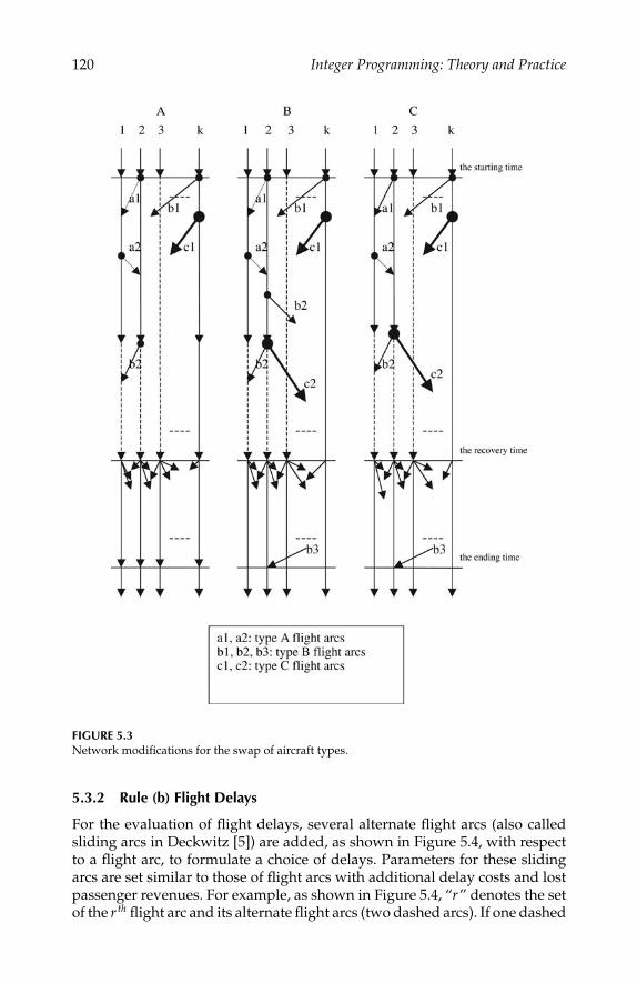
P1: shibu/Vijay

August 12, 2005 10:24 1914 1914˙C005


FIGURE 5.3Network modifications for the swap of aircraft types.

5.3.2 Rule (b) Flight Delays

For the evaluation of flight delays, several alternate flight arcs (also calledsliding arcs in Deckwitz [5]) are added, as shown in Figure 5.4, with respectto a flight arc, to formulate a choice of delays. Parameters for these slidingarcs are set similar to those of flight arcs with additional delay costs and lostpassenger revenues. For example, as shown in Figure 5.4, “r” denotes the setof the r th flight arc and its alternate flight arcs (two dashed arcs). If one dashed

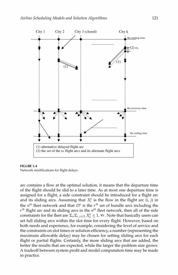
P1: shibu/Vijay

August 12, 2005 10:24 1914 1914˙C005


(1) alternative delayed flight arc(2) the set of the rth flight arcs and its alternate flight arcs

City 1 City 2 City 3 (closed) City k

the starting time

the recovery time

the ending time

(1)(1)

(2) rth

FIGURE 5.4Network modifications for flight delays.

arc contains a flow at the optimal solution, it means that the departure timeof the flight should be slid to a later time. As at most one departure time isassigned for a flight, a side constraint should be introduced for a flight arcand its sliding arcs. Assuming that Xn

ij is the flow in the flight arc (i, j) inthe nth fleet network and that Dn

r is the r th set of bundle arcs including ther th flight arc and its sliding arcs in the nth fleet network, then all of the sideconstraints for the fleet are ni, j∈Dr Xn

ij ≤ 1, ∀r . Note that basically users canset full sliding arcs within the slot time for every flight. However, based onboth needs and experience, for example, considering the level of service andthe constraints on slot times or solution efficiency, a number (representing themaximum allowable delay) may be chosen for setting sliding arcs for eachflight or partial flights. Certainly, the more sliding arcs that are added, thebetter the results that are expected, while the larger the problem size grows.A tradeoff between system profit and model computation time may be madein practice.

P1: shibu/Vijay

August 12, 2005 10:24 1914 1914˙C005


5.3.3 Rule (c) Modification of Multi-Stop Flights

Some uneconomic segments in a multi-stop flight may be suitably canceledto improve system profits when the aircraft are not enough for service, due toa schedule perturbation. To evaluate the cancellation of one-stop flight seg-ments, this research suggests an extension of the modeling technique by Simp-son [14]. As shown in Figure 5.5, Xn

ij , Xnjk, and Xn

ik stand for a nonstop flightfrom i to j, from j to k, or from i to k respectively in the nth fleet network. Xn

ijk

stands for a one-stop flight from i to j to k in the nth fleet network. In the tech-nique proposed by Simpson [14], Xn

ik is an addition. As introduced by Simpson[14], two nonstop segments (Xn

ij and Xnjk) are bridged by a one-stop arc (Xn

ijk ).A dummy node (a or b) is placed on flight (i, j) and flight ( j, k). This con-struction allows either (i, j) or ( j, k) segments to be operated independentlyas nonstop flights. Any previous arrivals at j cannot use the attractive “one-stop” arc joining the two flights. There are two cost arcs created for use if theflights operate independently. If the flights are connected, the Xn

ij flow directlytransfers to the Xn

ijk flow and receives an additional benefit of Rnik for doing so.

This model, however, does not consider the passenger demand from i to k.To evaluate the decomposition of a one-stop flight into complete nonstop

flights, this research introduces another nonstop segment,Xnik, and a side

constraint. Firstly, since the flight segment from i to k can be chosen at mostonce, that is, the sum of Xn

ik and Xnijk can be at most one, an additional constraint,

n(Xnik + Xn

ijk) ≤ 1, should be added.If Xn

ik has flows (should be 1), then Xnijk should be zero, meaning that the

one-stop flight from i to j to k is not served. Similarly, if Xnijk has flows (should

be 1), then Xnik should be zero, meaning that the passenger demand from i to k

i kj

Un=1Cn=0

a

bUn=1Cn=0

Cnbk

Cnik

Cnijk

ONE STOPARC

Cnaj

Cnaj= -Rnij+DCnijCnbk= -Rnjk+DCnjkCnik= -Rnik+DCnikCnijk= -Rnik+Cnaj

Rn: revenueDCn: operation costUn: arc flow upper bound

FIGURE 5.5Network modifications for a one-stop flight arc.

P1: shibu/Vijay

August 12, 2005 10:24 1914 1914˙C005


has been served by the one-stop flight i to j to k, and there is no need forproviding the nonstop flight from i to k. Note that the arc cost of Xn

ik is theflight cost minus the passenger revenue obtained on the nonstop flight fromi to k; all other arc costs are the same as those mentioned in Simpson [14].Similar to rule (b), users can evaluate all or part of the one-stop flights for theirneeds in practice. To reduce the model’s complexity, this research focuses onthe scheduling of nonstop and one-stop flights. Modifications for two-stopor more-stop flights can be considered in future research.

5.3.4 Rule (d) Ferrying of Idle Aircraft

This rule uses ferry flights to relocate idle airplanes of the same type to whereand when the system needs them for the best routing. As shown in Figure 5.6,position arcs with ferry flight costs are systematically added. For example, ifthere is a flow in the arc (b, s), it means that an aircraft should be relocated,

(1) position arc(2) gap for reposition(3) position arc for relocating aircraft back to normal

City 1 City 2 City 3 (closed) City k

(3)(3)

the starting time

the recovery time

the ending time

b

s(1)

(1)

(2)

(2)

FIGURE 5.6Network modifications for the ferrying of idle aircraft.

P1: shibu/Vijay

August 12, 2005 10:24 1914 1914˙C005


via a ferry flight from city 1 to city 2, when the perturbation begins. Note thatferry arcs should not be connected to the airport when it is closed. As in rules(b) and (c), users can add full position arcs into the network, or, they mayadd position arcs whenever and wherever they feel it to be suitable for thepossible relocation of airplanes. The model will then determine the optimalsolution. Obviously, the more position arcs that are added, the better theeffects of the ferry flights expected, while the larger the network size grows.A tradeoff between system profit and model computation time may be madein practice. No additional side constraints, but additional arcs are generatedin this modification.

Although modifications of the basic model for rules (b), (c), and (d) in eachfleet network are referred to in Yan and Lin [22], if rule (a) is applied togetherwith rule (b), then, because at most one departure time is assigned for a flight, aside constraint should be introduced for a flight arc and its alternate flight arcsamong all associated fleet networks to ensure that at most one flight is served.Similarly, if rule (a) is applied together with rule (c), then the additional sideconstraint mentioned in Yan and Lin [22] should be extended across all theassociated fleet networks. Besides, to ensure that each nonstop flight (whichis modified from a one-stop flight) is served at most once, a side constraintshould be introduced for each nonstop flight across all the associated fleetnetworks.

5.4 Solution Methods

The aforementioned models are formulated as pure network flow problems,network flow problems with side constraints, or multiple commodity networkflow problems. As in the basic model, a strategic model, not including rule(a), can be characterized as a single-fleet scheduling model, because any fleetnetwork is independent of the other fleet networks. Thus, the basic model, in-corporating rules (b), (c), or (d), can be formulated as pure network flowproblems or network flow problems with side constraints. Moreover, the basicmodel incorporated rule (a) and any of rules (b), (c), and (d) can be formulatedas multi-commodity network flow problems. These models are designed tohave optimal solutions, so that in actual applications they do not generateinfeasible or unbounded solutions (Yan and Lin [22]). Numerous methods arecapable of solving the pure network flow problem, including the out-of-kilteralgorithm, the network simplex method, the cost scaling algorithm and theright-hand-side scaling algorithm (Ahuja et al. [1]). This research suggestsusing the network simplex method to solve pure network flow problemsdue to its demonstrated efficiency, see Ahuja et al. [1] or Kennington andHelgason [12].

Since the network flow problems with side constraints and the multiplecommodity network flow problems are characterized as NP-hard, (see Gareyand Johnson [8]), traditional exact integer solution techniques are applicable,

P1: shibu/Vijay

August 12, 2005 10:24 1914 1914˙C005


for example, the branch-and-bound or the cutting planes. This research, how-ever, suggests using a Lagrangian relaxation with subgradient methods (LRS)for an approximation of the near-optimal solutions in order to avoid a longcomputation time for solving realistically large problems.

LRS is known for its fast convergence and efficient allocation of memoryspace (Fisher [7]). The LRS process is addressed as follows: By dualizingthe side constraints or the bundle constraints with a Lagrangian multiplier,we produce a Lagrangian problem that is easy to solve and whose optimalobjective is a lower bound (for minimization problems) on the optimal valueof the original problem. We then use a Lagrangian heuristic to find a feasiblesolution whose objective is an upper bound (for minimization problems) onthe optimal value of the original problem. To reduce the gap between theupper bound and the lower bound, we modify the Lagrangian multiplierusing a subgradient method, then solve for another lower and upper bound.Better bounds are updated. The process is repeated until the gap is convergedto within 0.1% of error.

Since the proposed network flow problem with side constraints is a specialcase of the proposed multiple commodity network flow problem, we intro-duce the LRS on the basis of the latter problem. The detailed application ofthe LRS in this research is summarized below in three parts.

(5.1) A lower bound for each iterationThe side constraints are relaxed by a nonnegative Lagrangian multiplier andare added to the objective function, resulting in a Lagrangian program whichcontains several independent pure network flow problems. Each pure net-work flow problem can be solved using the network simplex method and thesum of the optimal objective values can be proven to be the lower bound ofthe original problem (Fisher [7]).

(5.2) An upper bound for each iterationA Lagrangian heuristic is developed to find a feasible solution (an upperbound of the optimal solution), from the lower bound solution (typically aninfeasible solution), for each iteration. If a certain side constraint is violated,there should be at least two flight arcs in this set of side arcs with positive flow,which is equal to one. We choose the arc from among them with the largest arccost (after being modified by LR), to reduce its flow from one to zero. In orderto maintain the flow conservation on the arc’s tail and head, we find the leastcost flow augmenting path from this arc’s tail to the arc’s head in the associatedfleet network by a modified label correcting algorithm (Powell [13]), andaugment a unit of flow through the path; thus, we reduce it by one unit ofbundle flow, surely increasing the objective value. Any arc flow involvedwith side constraints cannot be increased during the flow augmentation toprevent the violation of other side constraints. If the side constraint is not yetsatisfied, we choose another arc with the next highest cost from this set toreduce by another unit of bundle flow until this side constraint is satisfied.If all the side constraints are scanned and modified to become feasible, thenwe have found a feasible flow. Otherwise, we discard the upper bound from

P1: shibu/Vijay

August 12, 2005 10:24 1914 1914˙C005


this iteration. Such a situation, however, was not found in the case studypresented in Section 5.5. Note that since the networks are designed to havefeasible solutions, we can find an initial upper bound (corresponding to theinitial feasible solution) at the beginning of the algorithm.

(5.3) Solution process:

The solution steps are listed below:

Step 0: Set the initial Lagrangian multipliers.Step 1: Solve the Lagrangian problem optimally using the network simplex

method to get a lower bound. Update the lower bound.Step 2: Apply the Lagrangian heuristic to find an upper bound and update

the upper bound.Step 3: If the gap between the lower bound and the upper bound is within a

0.1% error, stop the algorithm.Step 4: Adjust the Lagrangian multipliers using the subgradient method

(Camerini et al. [2]).Step 5: Set k = k + 1. Go to Step 1.

Because the solutions mentioned above are fleet flows and are incapable ofexpressing the route of each airplane, we suggest using a flow decompositionmethod (Yan and Lin [22]) to decompose the link flows in each fleet networkinto arc chains, with each arc chain representing an airplane’s route with theassociated aircraft type in the perturbed period. If some airplanes’ routes aredifferent from their original ones, flight swaps of the same aircraft type shouldbe done for these aircraft. Note that according to a major Taiwan airline car-rier, the swap cost for aircraft of the same type in its operations is small andcan be omitted. Thus a suitable aircraft swap does not cause deterioration inthe system performance. Also note that the arc chains may not be unique.When applying the models, the SOC scheduling group may solve several arcchain patterns, then send them to other groups for the application of aircraftmaintenance and crew scheduling constraints. Hence, there will be more op-tions for the SOC to choose the best routing and a satisfactory solution forall groups could be relatively easy to find. Even if all the patterns are infeasi-ble, then instead of revising only one schedule, as is done currently, severalalternate patterns with the same best profit would provide more flexibilityfor schedule revisions. Thus, both the scheduling process and the quality ofa schedule could be improved. However, more practical arc chains can bestudied in the future in order to meet the regulations for aircraft maintenanceor crew scheduling.

5.5 Case Study

To test how well the models may be applied in real world, we demonstratea case study based on data from a major Taiwan airline’s international op-erations (China Airlines [3]). There are 24 cities involved in its operations.

P1: shibu/Vijay

August 12, 2005 10:24 1914 1914˙C005


The flight timetable, used for testing, is rotated once a week and includes273 flights. About 20 percent of them are one-stop flights; the others are non-stop flights. There are several types of aircraft involved in its operations,including B737’s, AB3’s, AB6’s, MD11’s, B74L’s, B744’s and B747’s. For sim-plicity, we had three types of aircraft in this case study; type A indicates B737’s(3 airplanes) with 120 seats, type B includes AB3’s, AB6’s, MD11’s, and B74L’s(17 airplanes) with an average of 269 seats, and type C includes B744’s andB747’s (6 airplanes) with an average of 403 seats.

For ease of testing, as calculated in Yan and Lin [22], all the cost parameterswere set according to the airline’s reports and the Taiwan government regu-lations, with reasonable simplifications, refer to China Airlines [3] and CivilAeronautics Administration [4]. Note that according to the airline the swapcost for different aircraft types in its operations is very small compared to theflight cost. For simplicity, the swap cost between different fleets is assumedto be zero. Besides, since the airline has contracts with other airlines for trans-porting passengers under irregular operations, without additional charges,for simplicity, we assume that the additional charges, for reaccommodatingpassengers not getting on the smaller-sized aircraft for suitable flights to thesame destinations, are zero. Note that the cost typically affects the test results.Because the case study is only for demonstration purposes at the currentstage, the evaluation of the application of the models to actual operations isleft to future work.

For the simplification of strategy (b), we only add two alternate flight arcsafter each flight arc, each alternate flight denoting a delay of 30 minutes (inother words, we do not allow a delay of more than one hour in this test). Forstrategy (d), we add position arcs between every OD pair every 6 hours fromthe starting time to the recovery time. We assume that an airport (Taipei)is closed at 3:00 AM on Wednesday and will be reopened 8 hours later.Consequently, the starting time is 3:00 AM on Wednesday; the recovery timeis 11:00 AM on Wednesday and the ending time by definition is 6:20 AM onFriday.

Eighteen scenarios were done in this test. Scenario 1 (indicated as “Normal”)denotes a normal operation. Referred to Gershkoff [9], Scenario 2 (“SSP”)applies the successive shortest paths to randomly finding a series of aircraftroutes from the starting time to the ending time. The number of canceledflights can thus be calculated after fleet assignment. To assure that the fleetcan resume its normal operations after the ending time, ferry flights could beused in the assignment. Scenario 3 through Scenario 18 are associated with ourstrategic models. For example, Scenario “B” indicates the basic model (flightcancellations); “Ba” denotes the combined model for flight cancellations andthe swap of aircraft types; “Bb” denotes the combined model for flight cancel-lations and flight delays; “Bc” denotes the combined model for flight cancel-lations and the modification of multi-stop flights; “Bd” denotes the combinedmodel for flight cancellations and the ferrying of idle aircraft; and “Babcd” de-notes the combined model for flight cancellations, the swap of aircraft types,flight delays, the modification of multi-stop flights, and the ferrying of idle

P1: shibu/Vijay

August 12, 2005 10:24 1914 1914˙C005


aircraft. Models “B” and “Bd” are pure network flow problems and the othermodels are network flow problems with side constraints or multi-commoditynetwork flow problems. We used the network simplex method to solve thepure network flow problems and applied the Lagrangian relaxation-basedalgorithm to solve the network flow problems with side constraints or multi-commodity network flow problems. The convergence gap was set as 0.1% ofthe error. The same flow decomposition method (Yan and Lin [22]) was usedto decompose the link flows into arc chains in each fleet network, with eacharc chain representing an airplane’s route in the perturbed period.

We note that the SSP method is easy to implement using our networks. Inparticular, the label correcting algorithm (Ahuja et al. [1]) is applicable forsolving the fleet assignment. The SSP method used here is for the preliminaryevaluation of our models. Several C programs were developed for; (1) theanalysis of raw data, (2) the building of the basic model, (3) the developmentand solution of the strategic models, and (4) the output of data. The casestudy was implemented on an HP735 workstation. Sixteen strategic modelswere tested with problem sizes of up to 7,515 nodes and 29,355 arcs. All ofthe results show that the models could be useful for actual operations. Theresults are summarized in Table 5.1 and specifically analyzed as follows.

(1) The algorithms performed very well, indicating they could be usefulin practice. In particular, models “B” and “Bd” were optimally solved in twoseconds of CPU time. The other models converged within 0.1% of the error inat most 250 seconds of CPU time. Note that the CPU times for network gen-eration and data output in each scenario are relatively short compared withmodel solutions and can be neglected. This shows that the network simplex al-gorithm should be efficient for solving pure network problems, like “B” and“Bd”, and this research indicates that the proposed Lagrangian relaxation-based algorithm could also be efficient for solving the multi-commoditynetwork flow problems. Compared with the efficiency of the traditional ap-proach, the algorithms are superior.

(2) From column (10) in Table 5.1, we find that the multi-fleet schedulingmodels yield a higher profit than the single-fleet scheduling models. In par-ticular, all eight strategic models containing strategy “a” suggest that a fleetcan temporarily serve other types of flights in scheduling, so as to improvethe system profit. For example, three type C flights in Model “Ba” are servedby the type B fleet. The result for Model “Ba” (−72,896,930) is better thanthat for the basic model “B” (−72,691,067) which is a single-fleet schedulingmodel, an improvement of NT$ 205,863 (about 0.28%). For another example,six type B flights and three type C flights in Model “Babcd” are served by thetype A fleet, and the type B fleet respectively. The result for Model “Babcd”(−81,028,533) is better than that for Model “Bbcd” (−79,730,287), an improve-ment of NT$ 1,298,246 (about 1.63%). Similarly, Models “Bab”, “Bac”, “Bad”,“Babc”, “Babd”, and “Bacd” yield higher profits than “Bb”, “Bc”, “Bd”, “Bbc”,“Bbd”, and “Bcd” respectively. The improvements in profit are NT$ 223,466(0.28%), 407,149 (0.56%), 205,663 (0.28%), 1,602,025 (2.04%), 221,264 (0.28%),and 1,111,457 (1.53%) respectively.

P1: shibu/Vijay

August 12, 2005 10:24 1914 1914˙C005


TAB

LE5.

1

Res

ults

ofA

llSc

enar

ios

#N

odes

#L

ink

sC

omp

uta

tion

Tim

eO

bje

ctiv

eV

alu

eC

onve

rged

Gap

Sce

nar

io(s

ec)

#It

erat

ion

(NT

$)%

AB

CA

BC

#S

ide

Con

stra

ints

Nor

mal

——

−87

,674

,685

——

——

——

——

SSP

0.65

—−

47,9

06,4

44—

2,47

32,

473

2,47

35,

480

5,52

95,

483

—B

1.09

1−

72,6

91,0

670

2,47

32,

473

2,47

35,

480

5,52

95,

483

0B

a12

4.88

117

−72

,896

,930

0.1

2,47

32,

473

2,47

35,

548

5,54

85,

548

76B

b14

.29

11−

78,7

20,6

900.

042,

473

2,47

32,

473

5,54

85,

585

5,49

476

Bc

91.1

776

−72

,691

,067

0.1

2,47

32,

473

2,47

35,

480

5,64

15,

483

108

Bd

1.86

1−

72,8

35,6

030

2,47

32,

473

2,47

39,

530

9,57

99,

533

0B

ab39

.66

31−

78,9

44,1

560.

12,

473

2,47

32,

473

5,62

35,

623

5,62

376

Bac

250.

219

3−

73,0

98,2

160.

12,

505

2,50

52,

505

5,66

05,

660

5,66

010

8B

ad15

9.55

78−

73,0

41,2

660.

12,

473

2,47

32,

473

9,59

89,

598

9,59

876

Bbc

41.8

631

−78

,720

,690

0.02

2,47

32,

505

2,47

35,

488

5,69

75,

494

108

Bbd

62.8

425

−78

,924

,326

0.03

2,47

32,

473

2,47

39,

538

9,53

59,

544

76B

cd84

.14

37−

72,8

35,6

030

2,47

32,

505

2,47

39,

530

9,69

19,

533

108

Bab

c61

.14

45−

80,3

22,7

150.

082,

505

2,50

52,

505

5,73

55,

735

5,73

510

8B

abd

90.3

635

−79

,145

,591

0.01

2,47

32,

473

2,47

39,

673

9,67

39,

673

76B

acd

130.

5655

−73

,947

,060

0.03

2,50

52,

505

2,50

59,

710

9,71

09,

710

108

Bbc

d95

.237

−79

,730

,287

02,

473

2,50

52,

473

9,53

89,

747

9,54

410

8B

abcd

159.

7159

−81

,028

,533

0.07

2,50

52,

505

2,50

59,

785

9,78

59,

785

108

(con

tinu

ed)

P1: shibu/Vijay

August 12, 2005 10:24 1914 1914˙C005


TAB

LE5.

1(C

onti

nued

)

Res

ults

ofA

llSc

enar

ios

#Fl

igh

tsS

erve

db

y#

Mod

ified

Mu

lti-

stop

#O

rigi

nal

Flig

hts

Oth

erFl

eet

#C

ance

led

Flig

hts

#D

elay

edFl

igh

tsFl

igh

ts#

Ferr

yFl

igh

ts

Sce

nar

ioA

BC

B/A

C/B

AB

CA

BC

AB

CA

BC

#C

ance

led

Flig

hts

and

Flig

ht

Seg

men

tsTo

tal

Nor

mal

857

11—

——

——

——

——

——

——

——

SSP

857

11—

—3

253

——

——

——

16

131

B8

5711

00

214

20

00

00

00

00

18B

a8

5711

03

215

10

00

00

00

10

18B

b8

5711

00

28

20

40

00

00

00

12B

c8

5711

00

214

20

00

00

00

00

18B

d8

5711

00

214

20

00

00

00

20

18B

ab8

5711

03

29

10

40

00

00

10

12B

ac8

5711

23

413

10

00

00

01

10

18B

ad8

5711

03

215

10

00

00

00

30

18B

bc8

5711

00

28

20

40

00

00

00

12B

bd8

5711

00

28

20

30

00

00

50

12B

cd8

5711

00

214

20

00

00

00

20

18B

abc

857

116

24

12

09

00

30

11

010

Bab

d8

5711

23

29

10

30

00

04

20

12B

acd

857

113

32

131

00

00

00

41

016

Bbc

d8

5711

00

25

20

70

02

00

40

11B

abcd

857

116

35

11

010

00

10

43

08

P1: shibu/Vijay

August 12, 2005 10:24 1914 1914˙C005


(3) All of our models yield a higher profit than the SSP approach does. Thebest result (−81,028,533), for Model “Babcd”, is closest to the profit achievedin normal operations (−87,674,685). Model “Babcd” causes much less profitloss (NT$ 6,646,152) than using the SSP approach (NT$ 39,768,241). Thoughthe basic model, “B”, is the worst among the strategic models, its objective(−72,691,067) is significantly better than that of the SSP method (−47,906,444).We note that if more rules are incorporated to develop a strategic model, thenthe model will be more flexible for optimizing a temporary schedule, so thatsystem profits can be improved more. For example, the result for “Babcd” isbetter than that for “Babc”, which is better than “Bab”. The reader can seeother examples in Table 5.1. The reason that our models outperform the SSPmethod could be that although the SSP method cancels a series of uneco-nomic flights (3 type A, 25 type B, and 3 type C flights), it does not considerthe swapping of aircraft, the delaying of flights, the modification of multi-stop flights, the ferrying of idle aircraft, or a combination of these in adjustingthe schedule. Besides, its randomness for finding shortest paths neglects thecombinatorial complexity of systematic routings, possibly resulting in an infe-rior combination of aircraft routes. Through the effective adjustment of flightschedules or fleet routes, fewer flights are canceled (for example, only 7 (5 typeA, 1 type B, and 1 type C) flights are canceled in “Babcd”. Thus, higher profitsare achieved. We also find that the strategic models containing strategy “b”,for example, “Bb”, “Bab”, “Bbc”, “Bbd”, “Babc”, “Babd”, “Bbcd”, or “Babcd”yield significantly higher profits (more than 78,000,000) than other models(less than 74,000,000). This implies that a flight delay is an important andeffective strategy in schedule adjustment.

(4) Other than the profit considerations, the degree of schedule perturba-tion may be a criterion for carriers to evaluate levels of service for all strategicmodels. Typically the more flights perturbed, the higher the chance that thelevel of service is affected. Furthermore, the number of canceled flights (in-cluding one-stop flight segments) and delayed flights in the case study mayserve as an index of schedule perturbation. Although the influence on thelevel of service for flight cancellations and flight delays could be different,carriers may evaluate them separately, or use the technique of multiple cri-teria decision making. In this study, since a flight has at most a delay of onehour, its influence on the level of service could be omitted when comparedto a canceled flight. Thus, in terms of the level of service, “Babcd” could bethe best (7 canceled flights and 1 canceled one-stop flight segment, includ-ing 3 departure flights at Taipei during the closed period) and SSP the worst(31 canceled flights), as shown in Figure 5.2. Note that strategic models con-taining “b” canceled less flights (less than or equal to 12 flights and one-stopflight segments) than other models (more than 15). Consequently, consider-ing both profit and level of service, strategic models containing “b” performbetter than others. In particular, Model “Babcd” is the best of them all.

It should be noted that if a solution obtained from a strategic model, which isassociated with a large degree of schedule perturbation, might not be acceptedby carriers under real operating constraints (for example, crew availability or

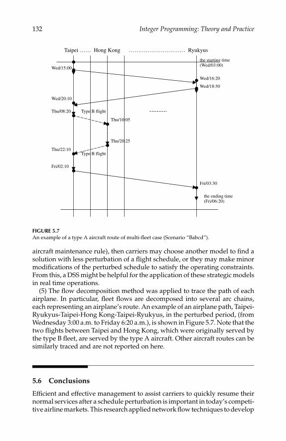
P1: shibu/Vijay

August 12, 2005 10:24 1914 1914˙C005


Taipei …… Hong Kong ………………………… Ryukyus

the starting time(Wed/03:00)

the ending time(Fri/06:20)

Wed/15:00

Wed/20:10

Wed/16:20

Wed/18:50

Thu/08:20

Thu/10:05

Fri/03:30

Type B flight

Type B flight

Thu/20:25

Thu/22:10

Fri/02:10

FIGURE 5.7An example of a type A aircraft route of multi-fleet case (Scenario “Babcd”).

aircraft maintenance rule), then carriers may choose another model to find asolution with less perturbation of a flight schedule, or they may make minormodifications of the perturbed schedule to satisfy the operating constraints.From this, a DSS might be helpful for the application of these strategic modelsin real time operations.

(5) The flow decomposition method was applied to trace the path of eachairplane. In particular, fleet flows are decomposed into several arc chains,each representing an airplane’s route. An example of an airplane path, Taipei-Ryukyus-Taipei-Hong Kong-Taipei-Ryukyus, in the perturbed period, (fromWednesday 3:00 a.m. to Friday 6:20 a.m.), is shown in Figure 5.7. Note that thetwo flights between Taipei and Hong Kong, which were originally served bythe type B fleet, are served by the type A aircraft. Other aircraft routes can besimilarly traced and are not reported on here.

5.6 Conclusions

Efficient and effective management to assist carriers to quickly resume theirnormal services after a schedule perturbation is important in today’s competi-tive airline markets. This research applied network flow techniques to develop

P1: shibu/Vijay

August 12, 2005 10:24 1914 1914˙C005


several systematic strategic models, combining various practical schedulingrules, to help carriers handle schedule perturbations resulting from the tem-porary closure of airports. These models were based on a basic model for-mulated as a time-space network from which various strategic models weredeveloped. These models minimize the schedule-perturbed time after inci-dents so that carriers can resume their normal services as soon as possible inorder to maintain their levels of service. In addition, these models combinethe swapping of aircraft, flight cancellations, flight delays, the modification ofmulti-stop flights, and the ferrying of idle aircraft in a combined and system-atic framework to effectively adjust a schedule following incidents, so that acarrier can maintain its profitability.

Mathematically, these strategic models were formulated as, pure networkflow problems, network flow problems with side constraints, or multiple com-modity network flow problems. We used the network simplex method to solvethe pure network flow problems and developed a Lagrangian relaxation-based solution algorithm to solve the network flow problems with side con-straints and multiple commodity network flow problems.

A case study of a major Taiwan airline’s operations was presented to test themodels. Sixteen strategic models and the SSP approach were tested, with sub-stantial problem sizes of up to 7515 nodes and 29355 arcs. Several C programswere developed to apply these models on an HP735 workstation. The algo-rithms performed very well. In particular, models “B” and “Bd” were solvedoptimally in two seconds of CPU time; other models converged within 0.1%of the error in at most 250 seconds of CPU time. We found that the multi-fleet scheduling models yield a higher profit than the single-fleet schedulingmodels. The improvements in profit for all multi-fleet strategic models weresignificant, between NT$ 205,663 and 1,602,025. The improved ratios fell be-tween 0.28 and 2.04%. This shows that a fleet can temporarily serve othertypes of flights in scheduling, so as to improve the system profit. We alsofound that all of our models yielded a higher profit than the SSP approachdoes. All of these results show that the models could be useful for actual op-erations. Since the case study is only for demonstration at the current stage,the evaluation of impact on the application of the models to actual operationsis left to future work.

Although this research is motivated by Taiwan airline operations, the mod-els developed here are not specific and could be applicable for operations inother areas. It might be possible that more than one airport is temporarilyclosed at the same time. To resolve this problem, the networks developed inthis research should be modified. In particular, the flow upper bounds of theflight arcs connected to these closed airports during the closed period are setto zero and the ending time of the network can be set as the last one calculatedamong all the closed airports. In addition, how to combine several smaller-type flights to form a larger-type flight is not considered in this research.Though it may make the modeling more complicated, it could be an effectivestrategy in multi-fleet operations and could be a direction for future research.Besides, the incorporation of other routing factors (for example, different or

P1: shibu/Vijay

August 12, 2005 10:24 1914 1914˙C005


multiple objectives involved in actual operations) and systematic models forhandling schedule perturbation caused by other types of incidents can be per-formed as well in future research. A computerized decision support systemuseful for users, to apply these strategic models in real time operations, couldalso be another direction of future research.

Finally, we note that the techniques and ideas used in this research couldbe similarly applied to more general daily airline operations control prob-lems, for example, a temporary limitation on airport operations from the FAAbecause of congestion, or other types of incidents (for example, temporaryaircraft shortage). Particularly, the time-space network could be used withmodifications on the starting time/the initial supply, the ending time/the fi-nal demand, and the nodes/arcs according to the planned schedule and theincident. The practical scheduling rules could also be added into the basicnetwork to develop various strategic models which should be formulated aspure network flow problems, network flow problems with side constraints, ormultiple commodity network flow problems. Then, the solution techniquesused in this research, with suitable modifications, may be applicable for solv-ing the problems. All of these could be topics for future research.

Acknowledgments

This research was supported by a grant from the National Science Council ofTaiwan. We thank China Airlines for providing the test problems.

References

1. Ahuja, R. K., Magnanti, T. L., and Orlin, J. B., Network Flows, Theory, Algorithms,and Applications, Prentice Hall, Englewood Cliffs, 1993.

2. Camerini, K., Fratta L., and Maffioli, F., On improving relaxation methods bymodified gradient techniques, Mathematical Programming Study, 3, 6, 1975.

3. China Airlines, China Airlines Annual Report 1992, Taipei, R.O.C., 1993.4. Civil Aeronautics Administration, CAA’s Fare Regulation for Using Airport Build-

ings, Land, and Other Relative Equipment, Ministry of Transportation and Com-munication, R.O.C ,1984.

5. Deckwitz, T. A., Interactive Dynamic Airplane Scheduling, Flight TransportationLaboratory Report R-84-5, Massachusetts Institute of Technology, 1984.

6. Etschmaier, M. M. and Rothstein, M., Estimating the Punctuality Rate Inherent inan Airline Schedule, Technical Report 19, Department of Industrial Engineering,University of Pittsburgh, 1973.

7. Fisher, M. L., The Lagrangian relaxation method for solving integer program-ming problems, Management Science, 27, 1, 1981.

8. Garey, M. R. and Johnson, D. S., Computers and Intractability: A Guide to the Theoryof NP-completeness, W. H. Freeman & Company, San Francisco, 1979.

9. Gershkoff, I., Aircraft Shortage Evaluator, presented at ORSA/TIMS JointNational Meeting, St. Louis, MO, 1987.

P1: shibu/Vijay

August 12, 2005 10:24 1914 1914˙C005


10. Jarrah, A.I., et al., A Decision Support Framework for Airline Flight Cancella-tions and Delays, Transportation Science, 27, 266, 1993.

11. Jedlinsky, D. C., The Effect of Interruptions on Airline Schedule Control,Masters thesis, Massachusetts Institute of Technology, 1967.

12. Kennington, J. L. and Helgason, R. V., Algorithms for Network Programming, JohnWiley & Sons, New York, 1980.

13. Powell, W. B., A review of sensitivity results for linear networks and a newapproximation to reduce the effects of degeneracy, Transportation Science, 23,231, 1989.

14. Simpson, R. W., Scheduling and Routing Models for Airline Systems, Flight Trans-portation Laboratory Report R-68-3, Massachusetts Institute of Technology,1969.

15. Teodorovic, D., A model for designing the meteorologically most reliable airlineschedule, European Journal of Operational Research, 21, 156, 1985.

16. Teodorovic, D., Airline Operations Research, Gordon and Breach Science Publish-ers, New York, 1988.

17. Teodorovic, D. and Guberinic, S., Optimal dispatching strategy on an airlinenetwork after a schedule perturbation, European Journal of Operational Research,15, 178, 1984.

18. Teodorovic, D. and Stojkovic, G., Model for operational daily airline scheduling,Transportation Planning and Technology, 14, 273, 1990.

19. Thengvall, B. G., Bard, J. F., and Yu, G., Balancing user preferences for aircraftschedule recovery during airline irregular operations, IIE Transactions on Oper-ations Engineering, 32, 181, 2000.

20. Thengvall, B. G., Yu, G., and Bard, J. F. Multiple fleet aircraft schedule recoveryfollowing hub closure, Transportation Research, 35A, 289, 2001.

21. Yan, S., Bernstein, D., and Sheffi, Y., Intermodal pricing using network flowtechniques, Transportation Research, 29B, 171, 1995.

22. Yan, S. and Lin, C., Airline scheduling for the temporary closure of airports,Transportation Science, 31, 72, 1997.

23. Yan, S. and Tu, Y., Multi-fleet routing and multi-stop flight scheduling for sched-ule perturbation, European Journal of Operational Research, 103, 155, 1997.

24. Yan, S. and Yang, D., A decision support framework for handling scheduleperturbation, Transportation Research, 30B, 405, 1996.

P1: shibu/Vijay

August 12, 2005 10:24 1914 1914˙C005

P1: shibu/Vijay

August 12, 2005 10:42 1914 1914˙C006

6Determining an Optimal Fleet Mixand Schedules: Part I — Single Sourceand Destination

Hanif D. Sherali and Salem M. Al-Yakoob

CONTENTS

6.1 Introduction: Problem Description . . . . . . . . . . . . . . . . . . 1376.2 Related Literature . . . . . . . . . . . . . . . . . . . . . . . . . . . . 1396.3 Modeling Preliminaries . . . . . . . . . . . . . . . . . . . . . . . . 143

6.3.1 Problem Notation and Assumptions . . . . . . . . . . . . . 1436.3.2 Penalty Functions . . . . . . . . . . . . . . . . . . . . . . . . 144

6.4 Model Development . . . . . . . . . . . . . . . . . . . . . . . . . . 1456.4.1 Model Variables . . . . . . . . . . . . . . . . . . . . . . . . . 1466.4.2 Model Constraints . . . . . . . . . . . . . . . . . . . . . . . 1476.4.3 Objective Function . . . . . . . . . . . . . . . . . . . . . . . 1486.4.4 Overall Model Formulation . . . . . . . . . . . . . . . . . . 149

6.5 An Aggregate Formulation AVSP for Model VSP . . . . . . . . . . 1506.5.1 Formulation of Model AVSP . . . . . . . . . . . . . . . . . . 150

6.5.1.1 Objective Function and Constraints . . . . . . . . 1526.5.1.2 Extracting Schedules for Individual Vessels . . . . 152

6.6 Computational Results and Rolling Horizon Heuristics . . . . . . 1536.6.1 Computational Experience in Solving

Models VSP and AVSP . . . . . . . . . . . . . . . . . . . . . 1536.6.2 Rolling Horizon Algorithms . . . . . . . . . . . . . . . . . . 1546.6.3 Comparison with an ad-hoc Scheduling Procedure . . . . . 157

6.7 Summary, Conclusions, and Future Research . . . . . . . . . . . . 159References . . . . . . . . . . . . . . . . . . . . . . . . . . . . . . . . . . . 160

6.1 Introduction: Problem Description

Efficient scheduling of oceanic transportation vessels presents serious chal-lenges to concerned decision-makers due to the complexity of the operationand the potential savings that can be attained. A vessel usually costs tens of

137

P1: shibu/Vijay

August 12, 2005 10:42 1914 1914˙C006


millions of U.S. dollars with daily operational costs amounting to tens of thou-sands of U.S. dollars. Chartering and spot-chartering of vessels is also veryexpensive and should be avoided to the extent possible. In general, large-scale vessel scheduling is very intricate and requires repeated revampingto accommodate changes in demand, market conditions, and weather effects.Manual approaches are often inefficient and expensive, and hence, it is imper-ative to utilize quantitative methods to generate and update vessel schedulesefficiently and in a timely fashion.

The problem that is studied in this chapter is concerned with the trans-portation of a product from a single source to a single destination. The nextchapter examines the case of multiple sources and destinations, along withthe option of leasing transshipment depots. For example, we might be in-terested in shipping crude oil from a refinery to a storage facility that has aknown demand structure defined by different daily consumption rates. Thedaily export from the source depends on the availability of the product at thesource, the availability of vessels, and the current storage level at the desti-nation’s storage facility. Consumption rates at the destination might not befixed during the entire time horizon and might vary based on, for example,seasonal considerations. The level of the product at the destination’s storagefacility is desired to lie within certain lower and upper bounds, and hence,daily penalties are imposed based on limited shortage or excess quantitieswith respect to these bounds.

Typically the organization that handles the transportation of the productfrom the source to the destination owns vessels of different types, where eachtype is characterized by the vessel size, speed, loading and unloading times,etc. Moreover, there are vessels that are available for chartering during all orpart of the time horizon. Spot-chartering is also available if desired, wherebya vessel is chartered for a particular voyage or voyages, not for a period oftime. In this case, all operating costs are undertaken by the vessel owner. (Seefor example, Rana and Vickson [24].)

The organization aims to satisfy demand requirements at a minimum over-all cost that is comprised of operational expenses, penalties resulting fromexceeding lower and upper storage levels, and chartering expenses. This re-quires an efficient utilization of the organization’s self-owned vessels, and aminimal reliance on chartered and spot-chartered vessels that tend to havehigh associated costs. The combinatorial nature of this problem makes themanual scheduling of vessels inefficient and costly because of unduly highresulting chartering and penalty expenses.

In this chapter, we develop mathematical models that generatecost-effectivevessel schedules in a timely fashion. The problem described above is faced bymany oil companies such as the Kuwait Petroleum Corporation (KPC), whichis required by agreed upon contracts to meet specified demands of crude oilthat vary based on daily consumption rates at a given destination. The sin-gle source-destination vessel scheduling operation arises in many situations,for example, when large quantities of crude oil need to be transported fromKuwait to a destination located in Europe, North America, or Asia. In this case,

P1: shibu/Vijay

August 12, 2005 10:42 1914 1914˙C006

Determining an Optimal Fleet Mix and Schedules 139

the destination might be a single customer or a collection of customers thatare located within close proximities of each other. Hence, the single sourceand destination problem considered herein, although a special case of themultiple source and destination problem addressed elsewhere [31], is impor-tant in its own right and is frequently faced in practice.

6.2 Related Literature

Transportation routing and scheduling problems have been widely researchedin the literature, with a bulk of the published work dealing with vehiclerouting and scheduling problems. Vessel scheduling, in particular, has at-tracted the least attention among all transportation modes. Ronen [26, 27]highlighted a noticeable scarcity of published research dealing with design-ing, planning, and managing sea-borne transportation systems, and gave anumber of impediments associated with vessel-scheduling problems such asthe complexity and the high uncertainties associated with such problems.However, recently, there has been increasing interest in research related tomaritime transportation as evidenced, for example, by a special issue de-voted to this area in Transportation Science (Psaraftis [23]). Also, the book byPerakis [20] gives an overview of models for a number of problems related tofleet operations and deployment. For a comprehensive review on ship rout-ing and scheduling research conducted over the last decade, the reader mayrefer to Christiansen et al. [8].

In order to accurately model vessel routing and scheduling problems, novelmathematical formulations are often needed. Moreover, models for large-scale vessel scheduling problems are rather hard to solve due to complexconstraint structures that result from the operational intricacies of such prob-lems, and their inherent combinatorial characteristics arising from an explicitconsideration of the different components of the operation. Vessel schedulingcan therefore be an arduous and time-consuming task, and is often compli-cated by the dynamic nature of such problems. Yet, many organizations stilllargely handle their vessel scheduling problems only manually.

Typically there are three modes of operation in seaborne shipping: liner,tramp, and industrial (see, for example, Christiansen et al. [8] and Lawrence[17]). Liners operate based on a fixed published itinerary and schedule similarto bus or passenger train lines. Tramp ships operate like a taxi by followingthe available cargos. In industrial shipping, the cargo owner controls thefleet of ships. Accordingly, vessel routing and scheduling problems can bepartitioned into four categories: a) liner, b) tramp, c) industrial, and d) otherrelated models. The first three are not sharply defined or mutually exclusive,nor collectively exhaustive (Lawrence [17]); hence, the fourth category ofproblems captures applications that cannot be clearly classified as liner, tramp,or industrial. It is worth mentioning that water transportation routing andscheduling models mainly deal with the transport and delivery of cargo.

P1: shibu/Vijay

August 12, 2005 10:42 1914 1914˙C006


Considerably fewer models have been developed to tackle vessel routingand scheduling problems in the context of transporting passengers. This isa result of the fact that most vessels move cargo around the world, whilepassengers mainly travel by air or land.

The literature on modeling techniques and approaches for the liner ship-ping is fairly limited; however, in recent years an increased activity in this areahas become evident (see, for example, Christiansen et al. [8] and Lane et al.[16]). Powell and Perakis [22] formulated an integer programming model for afleet deployment problem. The objective of the model was to minimize the op-erating costs for a fleet of liner ships involved in various routes. It was shown,based on real liner shipping data, that substantial savings could be achievedvia using the proposed modeling approach. Note that the work of Powell andPerakis [22] was an extension to the work of Perakis and Jaramillo [19] andJaramillo and Perakis [13]. In the latter two papers, a linear programmingapproach was used to solve a fleet deployment problem. Cho and Perakis [6]investigated a fleet size and design of a liner routing problem for a containershipping company. The problem was formulated by generating a subset ofcandidate routes for the different ships a priori, and was then solved as a lin-ear program, where the columns represent the candidate routes. This modelwas also extended to a mixed-integer program that additionally incorporatesinvestment alternatives for expanding fleet capacity. Xinlian et al. [31] formu-lated a fleet planning model for a problem similar to that investigated by Choand Perakis [6]. The model aims to determine the ship types to add to theexisting fleet of ships as well as an optimal fleet deployment plan.

Datz et al. [9] developed a simple calculative method for scheduling a linerand suggested some techniques for evaluating the financial results of such aschedule. Nemhauser and Yu [18] studied a model for rail service that can beused for a liner problem. Dynamic programming was used to find the optimalfrequency of services that maximizes profit over the planning horizon. De-mand for service was a function of two variables, namely service frequencyand timing. Rana and Vickson [24] developed a deterministic mathematicalprogramming model for optimally routing a chartered container vessel. Theformulation involves nonlinearities, which were handled by converting thenonlinear problem into a number of mixed-integer programs. Benders’ de-composition was applied to the resulting mixed-integer programs, whereinthe integer network subprograms were solved by a specialized algorithm.Later, Rana and Vickson [25] extended their work in [24] by allowing multipleships. They formulated a mathematical programming model for a container-ship routing problem that determines the following: 1) an optimal sequenceof ports of call for each vessel, 2) the number of trips each vessel makes in theplanning horizon, and 3) the amount of cargo delivered between any two portsby each ship. The problem was solved by Lagrangian relaxation by decom-posing it into several sub-problems, one for each vessel. Each sub-problemwas further decomposed into a number of mixed-integer programs. For otherrelated literature on liner models, the reader may refer to Christiansen et al.[8] and Al-Yakoob [1].

P1: shibu/Vijay

August 12, 2005 10:42 1914 1914˙C006


Very little research has been conducted on the allocation, routing, andscheduling of tramp shipping (see Appelgren [2, 3]). Appelgren [2] discusseda ship scheduling problem obtained from a Swedish ship-owning company.In this problem, a ship-owning company was engaged in world-wide oper-ations involving a large number of vessels. A set of cargos were providedfor the planning period, which covered 2 to 4 months. The author designedan algorithm that used the Dantzig-Wolf decomposition method for linearprogramming, where the subprograms were modeled as network flow prob-lems and were solved by dynamic programming. The master program in thedecomposition algorithm was modeled as a linear program having only zero-one elements in the matrix and on the right-hand-side. This algorithm wastested on instances involving about 40 ships and 50 cargos.

Later, Appelgren [3] utilized integer programming methods to solve a ves-sel scheduling problem. The problem was to determine an optimal sequenceof cargos for each vessel in a given fleet during a specified time period. Thispaper was an attempt to deal with some of the shortcomings associated withthe technique used by the author in [2], where a decomposition algorithmwas used, which, however, produced nonintegral solutions that could not beinterpreted as valid schedules. To avoid fractional solutions, a branch-and-bound algorithm was developed, where the branching was performed on oneof the ”essential” noninteger variables and the bounds were computed bythe decomposition algorithm. A decision support system for both tramp andindustrial shipping was described in Fagerholt [10], where a heuristic hybridsearch algorithm was employed for solving such ship scheduling problems.

Since the problem under consideration can be classified as an industrialshipping problem, we present next some industrial scheduling literature thatis most closely related to our problem.

A vessel scheduling problem concerned with transporting crude oil fromthe Middle East to Europe and North America was considered by Brownet al. [5], who formulated a mixed-integer partitioning model and utilizedcolumn generation techniques to solve this problem. The demand structurewas specified by a sequence of cargos that needed to be delivered during theplanning horizon. The approach adopted by Brown et al. [5] attempted togenerate a partial set of complete feasible schedules (in a column generationframework), along with the generated schedules’ costs, and then utilized anelastic set partitioning programming model to derive a prescribed solution.This same problem was investigated by Perakis and Bremer [21] who alsoapplied a set partitioning approach to solve the problem. The work of Brownet al. [5] was extended in Bausch et al. [4] by allowing a shipload to have upto five products. A similar set partitioning approach to that of Brown et al. [5]was used by Bausch et al. [4] to solve the problem.

Sherali et al. [30] presented mixed-integer programming models and spe-cialized rolling horizon algorithms for an oil tanker routing and schedulingproblem to ship various products from one source to different destinations.The demand structure that was investigated by Sherali et al. [30] was deter-mined by the total demand for each product at each destination, along with

P1: shibu/Vijay

August 12, 2005 10:42 1914 1914˙C006


the respective sub-demand that was required to be satisfied within agreed-upon time intervals. It was assumed that some vessels could carry more thanone product. The modeling approach adopted in Sherali et al. [30] as well asin this chapter differs from the modeling approach of Brown et al. [5] in that itcombines the process of constructing and selecting feasible schedules at once.

Ronen [28] proposed a mixed-integer programming model and a cost-basedheuristic procedure for a vessel transportation problem that is similar to theone considered in this chapter. The approach adopted by Ronen [28] separatesthe solution of the problem into two stages. The first stage determines the slateof shipments to be made, and the second stage generates vessel schedules. Incontrast, the models developed here decide upon the fleet size mix as well asthe detailed vessel schedules all together. Another application within the oilindustry, which involves the transport of refined oil products from a refineryto several depots, was investigated by Scott [29]. A Lagrangian relaxationapproach was adopted to generate a set of potentially good schedules, andan enhanced version of Benders’ decomposition was used to decide upon anoptimal schedule from within the generated set of schedules. Fagerholt andChristiansen [11] studied a multi-product scheduling problem similar to theone presented by Bausch et al. [4]. However, in this paper, the authors as-sumed that each ship in the fleet is equipped with a flexible cargo hold thatcan be partitioned into many holds in a specified number of ways. A setpartitioning approach was utilized by the authors for this problem and a de-tailed algorithm for finding optimal schedules for the individual ships wasdescribed in Fagerholt and Christiansen [12]. An inventory-routing problemwas studied by Christiansen [7], which attempts to attain a degree of balancein the ammonia supply at all producing and/or consuming company-ownedplants around the world.

A ship scheduling problem that does not clearly fall into liner, tramp, or in-dustrial shipping was investigated by Koenigsberg and Lam [14] who studiedqueuing aspects for a small system of liquid gas tankers operating in closedroutes between a small number of terminals. For any particular system, theirmodel provides the expected number of ships at each stage, the expectednumber waiting in each stage, and most importantly, the expected waitingtime at ports. Exponential service time distributions were used; however, aseries of parallel simulation computations were also employed to analyze theimpact of other distributions. Later, Koenigsberg and Meyers [15] extendedthe work of Koenigsberg and Lam [14] by developing an analytical model ofa system having two independent fleets that share a common loading port.Exponential distributions of service times were used in all queuing stages. Theauthors used a simulation program to investigate the behavior of the systemwhen the service time distributions were not exponential and demonstrated agood level of conformity between the simulation and the analytical results forexponential distributions.

For further details on vessel routing and scheduling problems and models,the reader may refer to Al-Yakoob [1], Christiansen [8], Perakis [20], andRonen [26, 27].

P1: shibu/Vijay

August 12, 2005 10:42 1914 1914˙C006


Although many vessel scheduling problems and models have been discuss-ed in the aforementioned literature, none of these fully address the peculiaraspects of the problem considered in this chapter. The specific nature of thedemand structure and the consideration of different vessel types and costcomponents require novel mathematical formulations and solution methodsto accurately model the problem and to derive solutions in a manner thatcan be practically implemented. The remainder of this chapter is organizedas follows. The next section provides a detailed description of the problem. Amixed-integer programming model is then developed in Section 6.4, and sub-sequently, an aggregate reformulation of this model is derived in Section 6.5.Solution algorithms and computational results are presented in Section 6.6,along with a comparison with the ad-hoc scheduling procedure that is cur-rently in use at KPC. Finally, Section 6.7 provides a summary and some con-cluding remarks.

6.3 Modeling Preliminaries

This section introduces aspects of the problem that will be used to formulateinteger programming models in Section 6.4 and Section 6.5. In particular,Section 6.3.1 presents notation and assumptions, and Section 6.3.2 describesa function for computing penalties associated with exceeding certain lowerand upper allowable storage levels. For the reader’s convenience, a glossaryof notation (sequenced in order of appearance) is provided in Appendix A.

6.3.1 Problem Notation and Assumptions

Let h = 1, . . . , H index the days of the time horizon under consideration.Typically, a time horizon is associated with a contract to deliver the productfrom the source to the destination based on some given consumption ratesas discussed in Section 6.1. Therefore, the terms “time horizon” and “con-tract horizon” will henceforth be used interchangeably. Note that a contractmay be signed, and then another contract may be signed prior to the end ofthe first contract horizon. Suppose that there are T vessel types, indexed byt = 1, . . . , T . It is assumed that vessels of the same type have similar featuressuch as capacity, speed, loading and unloading times, etc. The capacity of avessel of type t is denoted by t and the total number of vessels of this typethat are available for use during all or part of the time-horizon is given by Mt

(note that Mt is composed of self-owned vessels in addition to vessels that areavailable for chartering). For a vessel type t ∈ 1, . . . , T, let n = 1, . . . , Mt

index all vessels of this type, and let Ot and C Ht = Mt − Ot respectivelydenote the number of self-owned vessels and the number of available vesselsof this type that can be possibly chartered. Accordingly, let n = 1, . . . , Ot andn = Ot + 1, . . . , Ot + CHt ≡ Mt respectively index self-owned vessels andvessels that are available for chartering of type t. Let us also denote O =T

t=1 Ot and CH = Tt=1CHt. Let $t,n be the cost (in U.S. dollars) of chartering

P1: shibu/Vijay

August 12, 2005 10:42 1914 1914˙C006


a vessel n of type t, for n = Ot + 1, . . . , Ot + CHt = Mt, and for each t ∈1, . . . , T. Let UTt,n be the maximum number of days vessel n of type t canbe used during the time horizon. This time restriction is typically needed formaintenance purposes.

Let Tt represent the time required to load a vessel of type t at the source,plus the time this vessel takes to travel from the source to the destination,unload time at the destination, and then travel back from the destinationto the source. We assume that there is a unique prescribed route from thesource to the destination, and likewise, from the destination to the source. LetTt = T1,t + T2,t, where T1,t is the time required to load a vessel of type t at thesource plus and then travel to the destination, and T2,t is the time required tounload at the destination and then travel back to the source. Vessels of the sametype are assumed to have equal values of Tt (and their splits), and this durationis also assumed to be independent of h; i.e., Tt is independent of the day the legstarts (weather effects are neglected). The values of Tt and its splits are derivedfrom the design speed of the vessels of type t. Let DCt,n denote the dailyoperational cost of vessel n of type t so that the total operational cost of vesseln of type t is given by Ct,n = Tt(DCt,n), which covers the round-trip expensesfrom the source to the destination, and is independent of the day the trip starts.

Let Q denote a production capacity or certain imposed quota of the productat the source. At the beginning of the time horizon, the storage level at thedestination is given by w. This level may represent a single storage facilityor a collection of storage facilities at the destination; however, for the sakeof modeling, we only deal with a combined aggregate storage level. Let SL1and SL2 denote the minimum and maximum desired levels, respectively, atthe destination’s storage facility, which should be maintained to the extentpossible in order to avoid penalties. Accordingly, letπ denote the daily penaltyfor each shortage or excess unit at the destination. The permitted shortageand excess quantities at the destination with respect to the desired levelsSL1 and SL2 to the extent given by A1 and A2, respectively. Let b1 = SL1 −A1 and b2 = SL2 + A2. Let U B > b2 be a sufficiently large upper bound on themaximum allowable storage level on any given day of the time horizon. Short-ages levels falling below b1 or in excess of b2 (up to UB), while permitted, arehighly undesirable, and incur a significantly greater penalty λ > π per unit.

Let Rj denote the expected consumption rate at the destination on day j ,for j = 1, . . . , H. The different daily consumption rates arise from possibleseasonal changes during the time-horizon, as well as from client-specific con-siderations. Thus, the total cumulative consumption at the destination overthe days j = 1, . . . , h is given by TCh = h

j=1 Rj .

6.3.2 Penalty Functions

The daily storage levels determine the overall penalty over the time horizon,being given by the summation of all daily penalties as described below. LetSh be the storage level on day h. Define Type I and Type II penalty functionsas follows:Type I penalty:PI (Sh) = π maximum 0, (SL1 − Sh), (Sh − SL2) if Sh ∈ [b1, b2]

P1: shibu/Vijay

August 12, 2005 10:42 1914 1914˙C006


and

Type II penalty:PII(Sh) =

π A1 + λ(b1 − Sh) if Sh ∈ (0, b1),π A2 + λ(Sh − b2) if Sh ∈ (b2, UB),

where π and λ > π are as defined above. Note that if Sh ∈ [SL1, SL2], thenthe storage level lies within the desired bounds and no penalty is induced. IfSh ∈ [b1, SL1) ∪ (SL2, b2], then a penalty is incurred based on the respectiveshortage or excess quantity. On the other hand, if Sh ∈ [0, b1) ∪ (b2, UB), thena sufficiently large additional penalty rate is imposed continuously beyondthat of PI (.) to indicate the undesirabity of such a storage level on any givenday of the time horizon.

PROPOSITION 6.1Let Sh = S1,h − S2,h − S3,h + S4,h + S5,h , (6.1)

where

SL1 ≤ S1,h ≤ SL2, 0 ≤ S2,h ≤ A1, 0 ≤ S3,h ≤ b1,(6.2)

0 ≤ S4,h ≤ A2, and 0 ≤ S5,h ≤ UB − b2.

DefineP(Sh) : [0, UB] → [0, ∞)as the linear penalty function:P(Sh) = π(S2,h + S4,h) + λ(S3,h + S5,h).Then any minimization objective formu-

lation that incorporates the termP(Sh) defined above along with (1.1) and (1.2) willautomatically enforce the sum of the type I and type II penalties PI (Sh) + PI I (Sh).

PROOF Noting that 0 < π < λ we have that for any Sh ∈ [0, UB), the corre-sponding representation of Shin terms of S1,h , S2,h , S3,h , S4,h , and S5,his deter-mined as follows, where in each case, the remaining (unspecified) variablesfrom this list have zero values. If Sh ∈ [SL1, SL2], then Sh = S1,h . If Sh ∈[b1, SL1), then Sh = S1,h − S2,h , where S1,h = SL1 and S2,h = SL1 − Sh , while ifSh ∈ (SL2, b2], then Sh = S1,h+S4,h , where S1,h = SL2 and S4,h = Sh−SL2. Like-wise, if Sh ∈ [0, b1), then Sh = S1,h − S2,h − S3,h , where S1,h = SL1, S2,h = A1,and S3,h = b1 − Sh , while if Sh ∈ (b2, UB), then Sh = S1,h + S4,h + S5,h , whereS1,h = SL2, S4,h = A2, and S5,h = Sh − b2. In each case, the function P(Sh)

is readily verified to impose the required Type I plus Type II penalties asdescribed above, and this completes the proof.

6.4 Model Development

In this section, we formulate a mixed-integer programming model for theprescribed vessel scheduling problem. The variables and constraints of themodel are respectively presented in Section 6.4.1 and Section 6.4.2, and the ob-jective function and the proposed mathematical model are respectively givenin Section 6.4.3 and Section 6.4.4.

P1: shibu/Vijay

August 12, 2005 10:42 1914 1914˙C006


6.4.1 Model Variables

Define the following sets of binary decision variables. Let

Xh,t,n =

1 if vessel n of type t departs the source toward thedestination on day h,

0 otherwise,

Since a vessel cannot be dispatched from the source on day h unless it isavailable on this day, another set of binary variables is defined as follows.Let

Yh,t,n =

1 if vessel n of type t is available at the source on day h,

0 otherwise.

Finally, in order to represent the chartering decisions, let

Zt,n =

1 if vessel n of type t is selected for chartering during(all or only part of) the time horizon,

0 otherwise.

A vessel may be chartered for the entire duration of the time horizon orfor only a specified subset of it, depending on its availability. The charteringexpense, denoted by $t,n for a vessel n of type t is incurred as a fixed-cost basedon the availability duration of this vessel, whenever it is chartered during aspecified interval of the time horizon, regardless of its usage during this timeinterval. The reason for this is that selected chartered vessels will be under thecontrol of the (leased-to) company (in our case, KPC) for the specified timeinterval, and the (leased-to) company is free to make any related dispatchingdecisions during this interval.

REMARK 6.1Note that subsets of these binary decisions variables are a priori known to beeffectively zero, i.e., inadmissible. The following are examples of such zerovariables. A vessel n of type t might not be available for use from the firstday of the time horizon. This occurs if this vessel is a self-owned vessel that isinvolved in a trip from a previously signed demand contract that will termi-nate sometime during the current time horizon. In other words, previous con-tracts might have committed certain vessels over durations concurrent withthe present contract horizon. Accordingly, suitable sets of variables shouldbe defined to be zero for the present contract horizon problem to signify theunavailability of such vessels. This might also happen if this vessel is a char-tered vessel that will become available sometime after the first day of thetime-horizon. In either case, the vessel availability variable Yh,t,n is set to zerountil this vessel becomes available at the source. Also, for a chartered vesseln of type t, the leasing conditions may specify some last operational day forthis vessel so that sufficient time is allowed for the leasing company to trans-fer this vessel to another organization or perform a scheduled maintenance.

P1: shibu/Vijay

August 12, 2005 10:42 1914 1914˙C006


In this case, the availability variable Yh,t,n is set to zero whenever h + Tt isgreater than that specified day. Note that naturally whenever Yh,t,n = 0, thenXh,t,n = 0 because a vessel is dispatched on a given day only if it is avail-able on that day. Let φX and φY denote the index sets of X and Y variables,respectively, that are restricted to be fixed at specified binary values by virtueof such considerations.

6.4.2 Model Constraints

The various constraints of the model are formulated as described in turnbelow.

(A) Representation of the destination’s storage level

The daily storage level of the product at the destination must remain within[b1, b2] to the extent possible as discussed in the previous section, and appro-priate daily penalties are imposed based on the specific levels of the storage.Representation of the storage level is given by the following constraints.

(C1) Sh = w +∑

t

∑n

∑h1:h1+T1,t∈1, ... ,h

t Xh1,t,n − TCh, ∀ h ∈ 1, . . . , H,

(C2) Sh = S1,h − S2,h − S3,h + S4,h + S5,h , ∀ h ∈ 1, . . . , H,where SL1 ≤ S1,h ≤ SL2, 0 ≤ S2,h ≤ A1, 0 ≤ S3,h ≤ b1, 0 ≤ S4,h ≤ A2, and0 ≤ S5,h ≤ UB − b2.

Constraint (C1) gives the storage level on day h based on the daily consump-tion rates and the shipments of the product that are delivered on or beforeday h. Constraint (C2) represents Sh in terms of S1,h , S2,h , S3,h , S4,h , and S5,h asdescribed in (1.1) and (1.2) so that appropriate penalties would be incurred inthe objective function based on this representation as stated in Proposition 6.1.

(B) Availabilities of vessels

The vessel availability constraints are given as follows:

(C3) Yh,t,n = Yh−1,t,n − Xh−1,t,n +∑

h1:h1+Tt=h

Xh1,t,n, ∀ h ≥ 2, t, n,

(C4) Xh,t,n ≤ Yh,t,n, ∀ h, t, n.

A vessel n of type t can be dispatched from the source to the destination onday h only if it is available at the source on that day. This vessel is availableat the source on day h if either the vessel was available at the source on theprevious day and it was not dispatched, or this vessel was not available thereduring the previous day but it arrived on the current day. On the other hand,this vessel is unavailable on day h at the source if it was available there on theprevious day and it was dispatched on that day (assuming that Tt ≥ 2 for allvessel-types t), or it was unavailable on the previous day and it did not arriveon the current day. Constraint (C3) examines the availability of vessel n oftype t at the source on day h by incorporating these cases, and then Constraint(C4) permits dispatching of vessels conditioned upon this availability.

P1: shibu/Vijay

August 12, 2005 10:42 1914 1914˙C006


(C) Chartering of vessel

The following constraint examines if a vessel n ∈ Ot + 1, . . . , Mt of type tis selected for chartering or not.

(C5) Yh,t,n ≤ Zt,n, ∀ h, t, n ∈ Ot + 1, . . . , Mt.

Hence, a vessel n ∈ Ot + 1, . . . , Mt that is available for chartering is usedonly if Zt,n = 1.

(D) Capacity restrictions and maintenance requirements

A production capacity or certain imposed daily quota might restrict the maxi-mum amount of the product that can be shipped to the destination on any dayof the time horizon. This restriction is represented by the following constraint.

(C6)∑

t

∑n

t Xh,t,n ≤ Q, ∀h.

Furthermore, the following constraint enforces that any vessel n of type tcan be used for at most UTt,n days during the time horizon since differentage vessels might have different usage allowances. This restriction might beneeded for maintenance purposes and is enforced by the following constraint.

(C7)∑

h

Tt Xh,t,n ≤ UTt,n, ∀t, n.

Other forms of scheduled maintenance restrictions can be also accommodatedin the model by setting certain X-variables to zero.

6.4.3 Objective Function

The objective function is composed of the following terms.

(a) Operational costs (both for self-owned and chartered vessels) givenby ∑

h

∑t

∑n

Ct,n Xh,t,n.

(b) Penalty costs resulting from shortage or excess levels at the desti-nation’s storage are given by the following term based on the rep-resentation stated in Proposition 1 above.

∑h

π [S2,h + S4,h] +∑

h

λ [S3,h + S5,h].

(c) The chartering expenses are given by∑

t

Mt∑n=Ot+1

$t,n Zt,n.

P1: shibu/Vijay

August 12, 2005 10:42 1914 1914˙C006


6.4.4 Overall Model Formulation

The objective function terms (a), (b), and (c) together with the constraints yieldthe following model for the Vessel Scheduling Problem (VSP). (All indices areassumed to take on only their respective relevant values.)

VSP:

Minimize∑

h

∑t

∑n

Ct,n Xh,t,n +∑

h

π [S2,h + S4,h]

+∑

h

λ [S3,h + S5,h] +∑

t

Mt∑n=Ot+1

$t,n Zt,n,

subject to

(C1) Sh = w +∑

t

∑n

∑h1:

h1+T1,t∈[1, ... ,h]

t Xh1,t,n − TCh, ∀ h,

(C2) Sh = S1,h − S2,h − S3,h + S4,h + S5,h , ∀h,

(C3) Yh,t,n = Yh−1,t,n − Xh−1,t,n +∑

h1:

h1+Tt=h

Xh1,t,n, ∀ h ≥ 2, t, n,

(C4) Xh,t,n ≤ Yh,t,n, ∀ h, t, n,

(C5) Yh,t,n ≤ Zt,n, ∀ h, t, n ∈ Ot + 1, . . . , Mt,(C6)

∑t

∑n

t Xh,t,n ≤ Q, ∀ h,

(C7)∑

h

∑t

Xh,t,n Tt ≤ UTt,n, ∀ t, n,

Xh,t,n ∈ 0, 1,∀ h, t, n, ifXh,t,n /∈ φX, and fixed at zero or one otherwise, Y1,t,n ∈0, 1, ∀ t, n, 0 ≤ Yh,t,n ≤ 1, ∀ h ≥ 2, t, n, if Yh,t,n /∈ φY, and fixed at zero or oneotherwise, 0 ≤ Zt,n ≤ 1, ∀t, n = Ot +1, . . . , Ot +CHt, Sh ≥ 0, SL1 ≤ S1,h ≤SL2, 0 ≤ S2,h ≤ A1, 0 ≤ S3,h ≤ b1, 0 ≤ S4,h ≤ A2, and 0 ≤ S5,h ≤ UB−b2, ∀ h.

REMARK 6.2Note that by Constraint (C3), the integrality of the Y-variables is guaranteedonce the integrality of the X-variables and the Y-variables correspondingto the first day of the time horizon is enforced. The integrality of the Z-variables is then automatically enforced by Constraint (C5) along with thefourth term of the objective function. This holds true since if a vessel n ∈Ot + 1, . . . , Ot + C Ht of type t is selected for chartering, then this vesselis used in at least one trip from the source to the destination, in which caseYh,t,n = 1 for some day h,and hence, the corresponding Constraint (C5) thenenforces Zt,n to also take on a value of one. On the other hand, if this vessel is

P1: shibu/Vijay

August 12, 2005 10:42 1914 1914˙C006


not selected for chartering, then Yh,t,n = 0 for all days of the time-horizon, inwhich case the most attractive value for Zt,n is zero based on the fourth termof the objective function.

In the next section, we derive an aggregated formulation of Model VSP,and in Section 6.6, we present a problem size analysis for both formulations.

6.5 An Aggregate Formulation AVSP for Model VSP

The vessel scheduling problem at hand can be alternatively formulated bydeciding upon the number of vessels of each type that are needed to be dis-patched every day instead of having to make dispatching decisions aboutindividual vessels. In this section, we derive an aggregated version of ModelVSP that retains the essential characteristics of the operation while being farmore computationally tractable than Model VSP. This formulation can beideally used for problem instances having relatively longer time horizons inorder to deal with the ensuing large number of binary variables.

6.5.1 Formulation of Model AVSP

Assume that the daily operational costs of vessels of a given type are thesame, and that the chartering expenses of all such vessels are identical. Incase the operational costs of vessels of the same type are not identical, thenwe take the average of all such costs, and likewise for the chartering expenses.However, if there are significant differences between these daily operationalcosts or between the chartering expenses, then we may accordingly partitiona vessel-type into various sub-types so that the assumed cost representationis adequate. Hence, let DCt denote the average daily operational cost of avessel of type t and let Ct = Tt (DCt).

Define xh,t as an integer variable that represents the number of vessels oftype t that are dispatched from the source on day h. Define yh,t to be aninteger decision variable that represents the maximum number of vesselsof type t that are available for dispatching from the source on day h. Asmentioned in Remark 6.1, vessels might become available for use at differentdays of the time horizon due to, for example, their involvement in trips fromprevious demand contracts that will terminate sometime during the currenttime horizon. Hence, we let Oh,t be the number of self-owned vessels of typet that will become available for use for the first time at the source on day hof the time horizon, and we let C Hh,t be the number of vessels of type t thatwill become available for chartering on day h of the time horizon. Let αh,t =Oh,t + CHh,t and note that Ot = h Oh,t and CHt = hCHh,t. Accordingly, welet zh,t be the integer variable that denotes the number of vessels of type tthat are actually selected for chartering on day h of the time horizon and let$h,t denote the average chartering cost of a vessel of type t that will becomeavailable for use on day h of the time horizon.

P1: shibu/Vijay

August 12, 2005 10:42 1914 1914˙C006


Let Ah,t be the subset of indices for vessels of type t (both self-owned andvessels available for chartering) that will become available for use at the sourcefor the first time on day h of the time horizon. Hence, for a given day h andvessel type t, we let UTh,t = n∈Ah,t UTt,n

αh,t, which basically gives the average

usage allowance for a vessel of type t that will become available for use forthe first time on day h of the time horizon. Accordingly, UTt = h UTh,t givesthe average usage allowance for a vessel of type t.

Note that in this aggregated model, the variable yh,t represents the maxi-mum number of vessels of type t that could be consigned on day h as neces-sary; the actual number used, and in particular the chartering decisions, aregoverned in this model via the dispatching variables xh,t. Similar to the indexsets φX and φY, we let φx and φy denote the index sets of x-and y-variables,respectively, that are a priori restricted to be zero, or fixed at some knownpositive integer values.

The aggregated model is formulated as stated below, where the S-variablesare defined as for Model VSP.

AVSP:

Minimize∑

h

∑t

Ctxh,t +∑

h

π [S2,h+S4,h] +∑

h

λ [S3,h + S5,h] +∑

h

∑t

$h,tzh,t,

subject to

(AC1) Sh = w +∑

t

∑h1:

h1+T1,t∈1, ... ,h

txh1,t − TCh, ∀ h,

(AC2) Sh = S1,h − S2,h − S3,h + S4,h + S5,h , ∀ h,

(AC3) yh,t = yh−1,t − xh−1,t +∑

h1:

h1+Tt=h

xh1,t + Oh,t + zh,t, ∀h ≥ 2, t,

(AC4) xh,t ≤ yh,t, ∀ h, t,

(AC5) y1,t = O1,t + z1,t , ∀ t,

(AC6)∑

t

txh,t ≤ Q, ∀ h,

(AC7.1) zt =∑

h

zh,t, ∀ h,

(AC7.2)∑

h

Tt xh,t ≤ UTt (Ot + zt), ∀ t,

xh,t ∈ 0, 1, . . . , Mt, ∀ h, t, if xh,t /∈ φx and fixed at zero or one otherwise,0 ≤ yh,t ≤ Mt, ∀ h, t, if yh,t /∈ φy and fixed at zero or one otherwise,

zh,t ∈ 1, . . . , C Hh,t, ∀ h, t,

Sh ≥ 0, SL1 ≤ S1,h ≤ SL2, 0 ≤ S2,h ≤ A1, 0 ≤ S3,h ≤ b1,

0 ≤ S4,h ≤ A2, and 0 ≤ S5,h ≤ UB − b2, ∀ h.

P1: shibu/Vijay

August 12, 2005 10:42 1914 1914˙C006


6.5.1.1 Objective Function and Constraints

The objective function of Model AVSP is similar to that of Model VSP, whichrepresents the total operational costs for both the self-owned vessels andthe chartered vessels, the penalties resulting from shortage or excess levelsat the destination, and the chartering expenses. Constraints (AC1), (AC2),(AC4), (AC6), and (AC7.2) used are basically representations of Constraints(C1), (C2), (C4), (C6), and (C7), respectively, in an aggregate sense. Note thatConstraint (AC7.1) is a definitional constraint that computes the total numberof vessels of type t that are actually selected for chartering. Constraint (AC3)

is a representation of (C3) in an aggregate sense, however, the right-hand-sideof (AC3) also accounts for the first-time availabilities of the self-owned andchartered vessels. Note that Constraints (AC5) in concert with Constraints(AC3) and (AC4) are sufficient to account for the chartered vessels.

Note that the parameters Oh,t and C Hh,t used in this model are necessarybecause, unlike as in Model VSP, we no longer maintain a track of individualvessels. The above reformulation adopts an aggregated approach as indicatedby the integer decision variables that represent the number of dispatched ves-sels (without any individual vessel identity) over the time horizon, in lieu ofusing the previous binary variables. This formulation of the problem is morecompact, however, at the expense of having to relax the individual vessel’stotal usage and downtime restrictions (C7) to (AC7.1), which now representsan aggregate usage constraint for vessels of type t, because we no longerspecifically account for each individual vessel’s activity. Likewise, for thecommissioned chartered vessels, we assume that these vessels are availablefor the duration of use as prescribed by the model solution. This relaxed con-straint needs to be dealt with separately while implementing the model-baseddecision. Note that the integrality of the y-variables is automatically enforcedbased on a similar reasoning as discussed in Remark 6.2 above.

REMARK 6.3Consider the following constraint.

(AC5.1) zt ≥

xh,t +

∑h1<h:

(h1+Tt)>h

xh1,t − Oh,t

, ∀ h, t.

Note that the right-hand-side of the Constraint (AC5.1) yields the number ofvessels of type t that are being used on day h beyond the self-owned numberof vessels Oh,t. Thus, this constraint can be used to tighten the continuousrelaxation of Model AVSP.

6.5.1.2 Extracting Schedules for Individual Vessels

A feasible schedule for individual vessels can be extracted from the solutionof Model AVSP as follows. Having solved Model AVSP the variable zh,t at

P1: shibu/Vijay

August 12, 2005 10:42 1914 1914˙C006


optimality specifies the number of vessels of type t that are needed for char-tering on day h, and hence, we can determine the fleet size mix. Then, we canbegin dispatching different vessels of type t on each day h based on the valuesof the x-variables. In this process, the downtime unavailabilities of variousvessels and the balancing of days for which the different vessels are put intoservice could be incorporated. It is worth mentioning that, in practice, thereis some flexibility in scheduling maintenance and in vessel usage constraints.Hence, this facilitates the conversion of the model solution to one that can beimplemented on an individual ship basis without perturbing the overall so-lution and its associated cost and while satisfying (C7.2) to the extent possible.

6.6 Computational Results and Rolling Horizon Heuristics

In this section, we present computational results related to solving ModelsVSP and AVSP based on ten test problems that represent various operationalscenarios. The test problems are given in Appendix B. Section 6.6.1 providescomputational experience for solving Models VSP and AVSP directly by theCPLEX package (version 7.5). In Section 6.6.2, we develop two rolling horizonheuristics to solve problem instances that cannot be solved directly via ModelAVSP. Finally, in Section 6.6.3, we present an ad-hoc procedure that is intendedto simulate a manual scheduling procedure used by KPC and the schedulesobtained via this procedure are compared against those derived via the pro-posed modeling approach.

Notationally, we will let P denote the linear relaxation of any model P . Theoptimal objective function value of model P will be denoted by v(P). The bestupper bound and lower bound found for model P will be respectively denotedby vUB(P)and vL B(P). All runs below are made on a Pentium 4, CPU 1.70 GHzcomputer having 512 MB of RAM using CPLEX-7.5, with coding in Java. Thetest problem instances are labeled as defined in Appendix B: Ii for i = 1, . . . ,10. The symbol “•” will be used to indicate that no meaningful solution of agiven model was obtained using CPLEX due to out-of-memory difficulties.

6.6.1 Computational Experience in Solving Models VSP and AVSP

Table 6.1 and Table 6.2 report computational results related to solving ModelsVSP and AVSP using CPLEX-MIP-7.5 based on the ten test problems.

REMARK 6.4The number of constraints and variables in Model AVSP are substantially lessthan the respective number of constraints and variables in Model VSP, as ob-served from Table 6.1 and Table 6.2. For example, the number of constraintsand variables for Model VSP based on test instance I10 are respectively givenby 10,451 and 11,126, while those for Model AVSP for this test instance are2,366 and 4,242, respectively. Note that these numbers are obtained fromCPLEX after performing necessary preprocessing and elimination steps.

P1: shibu/Vijay

August 12, 2005 10:42 1914 1914˙C006


TABLE 6.1

Linear Relaxation of Model VSPNonzero CPU Time

Ii Rows Columns Entries v(VSP) ($) (seconds)

I1 493 598 4,460 390,000 0.01I2 503 727 7,787 615,000 0.01I3 1,636 1,811 24,601 615,000 0.08I4 1,614 1,958 35,859 1,290,000 0.11I5 5,176 5,519 146,415 3,930,000 0.61I6 4,399 4,728 114,657 4,290,000 0.50I7 5,082 5,487 173,115 7,400,000 0.69I8 10,590 11,106 441,532 6,630,000 1.61I9 8,812 9,407 421,789 7,980,000 1.53I10 10,451 11,126 556,298 14,999,166 13.89

This will motivate the utilization of Model AVSP in concert with rolling hori-zon algorithms that are designed below to solve problem instances havingrelatively long time horizons.

REMARK 6.5Solutions for the linear relaxations of both Models VSP and AVSP were read-ily obtained for all the test problems. We were unable to obtain meaningfulsolutions for Model VSP for any of the test problems due to out-of-memorydifficulties. For Model AVSP, we were able to solve it directly only for testproblems I1, . . . , I4, while for test problems I5, . . . , I10, we encounteredout-of-memory difficulties before reaching meaningful solutions.

6.6.2 Rolling Horizon Algorithms

In this section, we present rolling horizon algorithms similar to thoseproposed in [30] to facilitate the derivation of good quality solutions withreasonable effort for the test problem instances that cannot be solved directly

TABLE 6.2

Statistics Related to Solving Model AVSPNonzero CPU Time CPU Time

Ii Rows Columns Entries v(AVSP)($) (seconds) v(AVSP)($) (seconds)

I1 105 235 688 390,000 0.00 420,000 0.01I2 205 477 2,273 615,000 0.02 660,000 6,363.16I3 342 682 3,990 615,000 0.01 660,000 0.02I4 519 1,039 8,696 1,459,166 0.03 1,500,000 0.06I5 698 1,394 15,198 4,520,000 0.03 ? 14,002.11I6 1,172 2,108 27,405 10,125,000 0.06 ? 310,593.03I7 1,173 2,199 33,700 7,765,000 0.08 ? 318,887.36I8 1,406 2,622 45,954 7,190,000 0.13 ? 105,854.48I9 2,061 3,689 81,638 9,260,000 0.25 ? 771,486.74I10 2,366 4,242 107,672 16,157,333 0.45 ? 39,559.61

P1: shibu/Vijay

August 12, 2005 10:42 1914 1914˙C006


via Model AVSP. These algorithms are based on a sequential fixing of integervariables and are presented below along with related computational results.Note that since optimal solutions of Model AVSP based on test problemsI1, . . . , I4 were obtained using CPLEX, we only apply the proposed rollinghorizon algorithms for test problem instances I5, . . . , I10.

Let AVSP(H, opt - gap) denote the relaxation of Model AVSP for whichintegrality is enforced only on the pertinent x-variables that correspond today 1 through day H of the time horizon, and an optimal solution is re-quired to be found within a tolerance “opt-gap” of optimality. Note thatv(AVSP(H, opt-gap)) provides a lower bound for problem AVSP, wherev(AVSP) ≤ v(AVSP(H, opt-gap)). Furthermore, increasing H and decreasingopt-gap will tighten this lower bound. Using the default CPLEX optimalitygap, we solved AVSP(H, opt-gap) for the largest possible integer n, whereH ≡ 10n ≤ H, such that a meaningful solution is obtained within a maxi-mum of 7 hours of run time. Let vLB = v(AVSP(H, opt-gap)) for the largestcomputationally feasible H as discussed above. Table 6.3 displays the resultsobtained.

(A) Rolling Horizon Algorithm RHA1

In Model AVSP, let the vector x be partitioned as (x1, x2, . . . , xH), where xh

denotes the vector of x-variables associated with the hth day of the time hori-zon. Let H1 be the length of the horizon interval for which the correspondingx-variables are restricted to be integer valued, and the remaining variablesare declared to be continuous. Accordingly, in a rolling-horizon framework,let H2 be the duration of the initial subset of this interval for which the deter-mined decisions are permanently fixed. Let KK = ((H − H1)/H2) + 1andlet AVSP(H1, H2, opt-gap, k), for k = 1, . . . , KK, denote Model AVSP havingthe following characteristics:

(a) xh is enforced to be integer valued for h ≤ H1 + (k − 1)H2, and isrelaxed to be continuous otherwise, ∀ h = 1, . . . , H.

(b) xh for h ≤ (k − 1)H2 is fixed at the values found from the solutionto Model AVSP(H1, H2, opt-gap, (k − 1)).

(c) The optimality gap tolerance for fathoming is set at opt-gap.

The rolling-horizon algorithm (RHA1) then proceeds as follows.

TABLE 6.3

Statistics Related to Solving v(AVSP(H, opt-gap))

Ii vLB ($) H (days) CPU Time (seconds)

I5 4,580,000 80 0.28I6 11,069,999 80 2,501.30I7 7,840,000 80 0.61I8 7,265,000 90 0.73I9 9,335,000 90 1.61I10 16,265,333 90 2.44

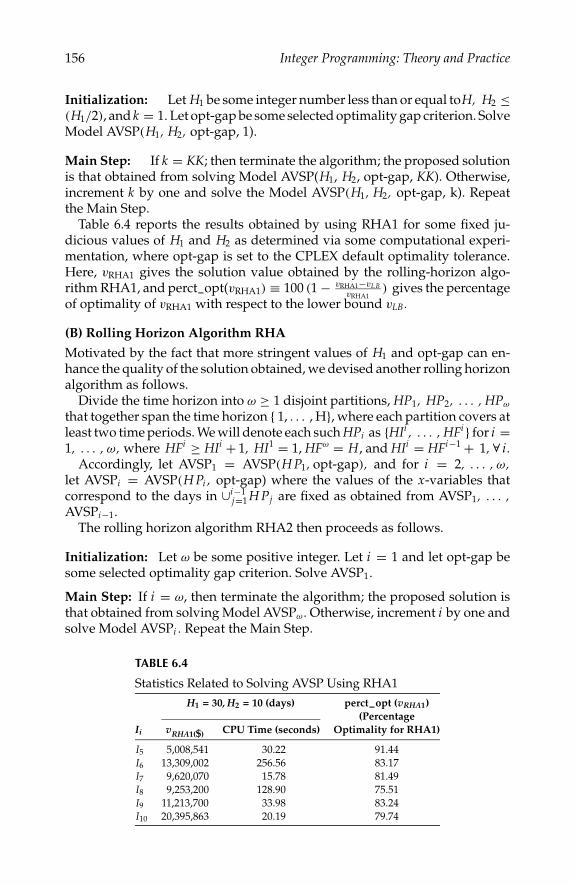
P1: shibu/Vijay

August 12, 2005 10:42 1914 1914˙C006


Initialization: Let H1 be some integer number less than or equal toH, H2 ≤(H1/2), and k = 1. Let opt-gap be some selected optimality gap criterion. SolveModel AVSP(H1, H2, opt-gap, 1).

Main Step: If k = KK; then terminate the algorithm; the proposed solutionis that obtained from solving Model AVSP(H1, H2, opt-gap, KK). Otherwise,increment k by one and solve the Model AVSP(H1, H2, opt-gap, k). Repeatthe Main Step.

Table 6.4 reports the results obtained by using RHA1 for some fixed ju-dicious values of H1 and H2 as determined via some computational experi-mentation, where opt-gap is set to the CPLEX default optimality tolerance.Here, vRHA1 gives the solution value obtained by the rolling-horizon algo-rithm RHA1, and perct_opt(vRHA1) ≡ 100 (1 − vRHA1−vL B

vRHA1) gives the percentage

of optimality of vRHA1 with respect to the lower bound vLB.

(B) Rolling Horizon Algorithm RHA

Motivated by the fact that more stringent values of H1 and opt-gap can en-hance the quality of the solution obtained, we devised another rolling horizonalgorithm as follows.

Divide the time horizon into ω ≥ 1 disjoint partitions, HP1, HP2, . . . , HPω

that together span the time horizon 1, . . . , H, where each partition covers atleast two time periods. We will denote each such HPi as HIi , . . . , HFi for i =1, . . . , ω, where HFi ≥ HIi + 1, HI1 = 1, HFω = H, and HIi = HFi−1 + 1, ∀ i.

Accordingly, let AVSP1 = AVSP(H P1, opt-gap), and for i = 2, . . . , ω,let AVSPi = AVSP(H Pi , opt-gap) where the values of the x-variables thatcorrespond to the days in ∪i−1

j=1 H Pj are fixed as obtained from AVSP1, . . . ,AVSPi−1.

The rolling horizon algorithm RHA2 then proceeds as follows.

Initialization: Let ω be some positive integer. Let i = 1 and let opt-gap besome selected optimality gap criterion. Solve AVSP1.

Main Step: If i = ω, then terminate the algorithm; the proposed solution isthat obtained from solving Model AVSPω. Otherwise, increment i by one andsolve Model AVSPi . Repeat the Main Step.

TABLE 6.4

Statistics Related to Solving AVSP Using RHA1H1 = 30, H2 = 10 (days) perct_opt (vRHA1)

(PercentageIi vRHA1($) CPU Time (seconds) Optimality for RHA1)

I5 5,008,541 30.22 91.44I6 13,309,002 256.56 83.17I7 9,620,070 15.78 81.49I8 9,253,200 128.90 75.51I9 11,213,700 33.98 83.24I10 20,395,863 20.19 79.74

P1: shibu/Vijay

August 12, 2005 10:42 1914 1914˙C006


TABLE 6.5

Statistics Related to Solving AVSP Using RHA2CPU CPU CPU

v(AVSP1) HF1 Time v(AVSP2) HF2 Time v(AVSP3) HF3 TimeIi ($) (days) (seconds) ($) (days) (seconds) ($) (days) (seconds)

I5 4,580,000 80 0.28 4,680,000 120 47.41 N/AI6 11,069,999 80 2,501.30 11,400,000 120 0.52 N/AI7 7,840,000 80 0.61 7,900,000 120 0.83 8,000,000 150 22.14I8 7,265,000 90 0.73 7,310,000 150 860.27 7,400,000 180 1.64I9 9,335,000 90 1.61 9,339,999 170 49.89 9,360,000 210 0.95I10 16,265,333 90 2.44 16,293,333 170 34.52 16,450,000 240 5.77

Let vRHA2 denote the solution value obtained by the rolling horizon algo-rithm RHA2, and let perct_opt(vRHA2) = 100(1 − vRHA2−vL B

vRHA2), which gives the

percentage of optimality of vRHA2 with respect to the lower bound vLB. More-over, let perct_imp(vRHA2, vRHA1) = 100( vRHA1−vRHA2

vRHA1), which gives the percent-

age of improvement in total cost of algorithm RHA2 over algorithm RHA1.Table 6.5 and Table 6.6 report statistics related to algorithm RHA2, whereopt-gap is set to the default CPLEX optimality gap.

Note that the sets of test problems I5, I6, and I7, . . . , I10 were solvedusing two and three partitions, respectively. Furthermore, algorithm RHA2produced better results than RHA1 for all the test problems under consider-ation. Note that the performance of these algorithms (particularly the latter)may be enhanced by using higher-grade computers that would permit fixingor relaxing fewer variables at each step.

6.6.3 Comparison with an ad-hoc Scheduling Procedure

In this section, we compare the performance of the proposed modeling ap-proach vs. an ad-hoc scheduling procedure that represents the processadopted by Kuwait Petroleum Corporation. Since chartering expenses arelarge relative to operational costs and penalties imposed for undesirable

TABLE 6.6

Statistics Related to Solving AVSP Using RHA2perct_opt (vRHA2) perct_imp (vRHA2, vRHA1)

Total (Percentage (PercentageCPU Time Optimality Improvement of

Ii vRHA2($) (seconds) for RHA2) RHA2 over RHA1)

I5 4,680,000 47.69 97.86 6.56I6 11,400,000 2,501.82 97.10 14.34I7 8,000,000 23.58 98.00 16.84I8 7,400,000 862.64 98.17 20.02I9 9,360,000 52.45 99.73 16.53I10 16,450,000 42.73 98.87 19.34

P1: shibu/Vijay

August 12, 2005 10:42 1914 1914˙C006


storage levels, this ad-hoc procedure attempts to fully utilize company-ownedvessels before resorting to chartered vessels, and operates as follows:

(A) Examine the first day of the time horizon, say h, on which deliv-ery of shipments is possible without exceeding SL2, and dispatchcompany-owned vessels for delivery on day h so that the total stor-age level on that day will not exceed SL2. This involves exploringvarious feasible departure days, and the usage of different combi-nations of vessels. This process is repeated for the company-ownedvessels, taking into account the availability of vessels during thedays of the time horizon, until it becomes impossible to do so.

(B) Repeat Step A, however, without exceeding b2, i.e., allowing for theType I penalty when the storage level lies within (SL2, b2].

(C) Repeat Step A, however, without exceeding UB, i.e., allowing forthe Type I and Type II penalties when the storage level lies within(SL2, UB].

(D) Now, if the storage level on any given day of the horizon is not be-low zero, then we are done, and hence, there is no need for charteredvessels. Otherwise, let hh be a day when the storage level becomesnegative, and select the smallest sized vessel that is available forchartering to be dispatched for delivery on a day in (hh − δ), whereδ is to be determined by the scheduler. Repeat this step as neces-sary, however, using the already selected chartered vessel(s). At eachpass through this process, if the storage level on any given day of thetime horizon is nonnegative, then we are done. On the other hand,if there exist no more chartered vessels while for some day we stillhave a storage level below zero, then no feasible solution is found.

Let AH denote the foregoing ad-hoc procedure. Table 6.7 presents some com-putational statistics for comparing schedules obtained via Procedure AH withthose generated by the proposed modeling approach. Here, vAH representsthe total cost of the solution obtained via AH and vmin gives the objective valueof the best solution obtained via the proposed modeling approach. Also, letperct_imp(vmin, vAH) = 100[( vAH−vmin

vAH)], which gives the percentage improve-

ment in the total cost of the schedules generated by the proposed modelingapproach over those obtained via the ad-hoc procedure.

Observe that for each of the test problems I1, . . . , I10, the overall cost ob-tained via the proposed modeling approach is often substantially better thanthe overall cost obtained via the ad-hoc procedure AH. For example, in testproblem I10, the improvement in total cost obtained via the modelingapproach over that obtained via the existing AH procedure is $47,090,000.Notice also that there is a large variance in the performance of the ad-hoc proce-dure AH vs. the proposed approach. The reason for this is two-fold. First,the AH procedure makes myopic decisions and is unable to recognize complexcompromises that sometimes need to be made for attaining an overall efficient

P1: shibu/Vijay

August 12, 2005 10:42 1914 1914˙C006


TABLE 6.7

Comparison of the ad-hoc Procedure AH vs. the ProposedModeling Approach

(Percentage Improvementof the Proposed Approach

over the Ad-hoc Approach)Ii vmin($) vAH($) perct_imp (vmin, vAH)

I1 420,000 720,000 41.66I2 660,000 720,000 8.33I3 660,000 2,480,000 73.38I4 1,500,000 3,940,000 61.93I5 4,680,000 6,720,000 30.35I6 11,400,000 42,178,000 72.97I7 8,000,000 10,880,000 26.47I8 7,400,000 8,282,000 10.65I9 9,360,000 56,450,000 83.42I10 16,450,000 24,140,000 31.85

solution. Second, because of such myopic decisions that unwisely use the self-owned vessel resources, the ad-hoc procedure often needs to resort to unneces-sary chartering of vessels, which is an expensive venture. On the other hand,the proposed modeling approach makes more effective and robust decisions.

6.7 Summary, Conclusions, and Future Research

In this chapter, we presented mixed-integer programming models for deter-mining an optimal mix of vessels of different types that are needed to transporta product from a source to a destination based on a stream of consumptionrates at the destination’s facility. Various cost components such as daily op-erational costs of vessels, chartering expenses, and penalties associated withundesirable storage levels are incorporated in the models. Such single source-destination vessel scheduling problems are faced by oil companies, for exam-ple, in which the product is crude oil, the source is a refinery facility, and thedestination is a storage location that belongs to a client. Problems of this typealso arise in practice where large quantities of crude oil need to be shippedfrom a country such as Kuwait to specific aggregated clusters of locations inEurope, North America, or Asia.

Due to the combinatorial nature of the problem, a manual scheduling ofvessels is often expensive and requires an inordinate amount of effort forconstructing and revamping vessel schedules. Therefore, it is imperative toutilize modeling approaches to advantageously compromise between thevarious cost components in order to avoid unduly high vessel charteringand penalty expenses. The proposed modeling approach enables the trans-porting organization to generate and revamp vessels’ schedules as frequently

P1: shibu/Vijay

August 12, 2005 10:42 1914 1914˙C006


as necessary and in a timely fashion. This approach also allows the organiza-tion to contemplate long-term plans regarding the size of the self-owned fleetand the need for chartered vessels.

The efficiency of the proposed modeling approach is assessed by com-paring it against an ad-hoc scheduling procedure that represents the actualscheduling of vessels in a related case study concerning Kuwait PetroleumCorporation (KPC). Using a set of ten realistic test problems, the results in-dicate that the proposed approach substantially improves upon the manualprocedure, resulting in savings ranging from $60,000 to $47,090,000.

The current manual practice at KPC suffers from a lack of robustness be-cause of the myopic nature of decisions made. Often, such decisions encumberthe self-owned vessels ineffectively, resulting in relatively large expenses forchartering additional vessels. On the other hand, the developed proceduredetermines near-optimal solutions more robustly within 97 to 99 percent ofoptimality.

This work can be extended to examine the cost effectiveness of simultane-ously investigating multiple sources and destinations instead of associatingspecific vessels with designated source-destination combinations. We can alsoexplore the impact of leasing temporary transshipment storage depots on theoverall chartering and penalty costs, whereby fewer chartered vessels mightneed to be acquired. These two extensions are the subject of a companionfollow-on paper [31].

Acknowledgments

This research work was supported by Kuwait University under ResearchGrant No. SM-06/02 and the National Science Foundation under ResearchGrant No. DMI-0094462. Special thanks to Mrs. Lulwa Al-Shebeeb forher contribution in the computational implementation of the solutionalgorithms.

References

1. Al-Yakoob, S.M., Mixed-integer mathematical programming optimization mod-els and algorithms for an oil tanker routing and scheduling problem, PhD. dis-sertation, Department of Mathematics, Virginia Polytechnic Institute and StateUniversity, Blacksburg, 1997.

2. Appelgren, L.H., A column generation algorithm for a ship scheduling problem,Transportation Science, 3, 53, 1969.

3. Appelgren, L.H., Integer programming methods for a vessel scheduling prob-lem, Transportation Science, 5, 64, 1971.

4. Bausch, D.O., Brown, G.G., and Ronen, D., Scheduling short-term marine trans-port of bulk products, Maritime Policy and Management, 25(4), 335, 1998.

5. Brown, G.G., Graves, G.W., and Ronen, D., Scheduling ocean transportation ofcrude oil, Management Science, 32, 335, 1983.

P1: shibu/Vijay

August 12, 2005 10:42 1914 1914˙C006


6. Cho, S.C. and Perakis, A.N., Optimal liner fleet routing strategies, Maritime Policyand Management, 23(3), 249, 1996.

7. Christiansen, M., Decomposition of a combined inventory and time constrainedship routing problem, Transportation Science, 3(1), 3, 1999.

8. Christiansen, M., Fagerholt, K., and Ronen, D., Ship routing and scheduling:status and prospective, Transportation Science, 38(1), 1, 2004.

9. Datz, I.M., Fixman, C.M., Friedberg, A.W., and Lewinson, V.A., A description ofthe maritime administration mathematical simulation of ship operations, Trans.SNAME, 493, 1964.

10. Fagerholt, K., A computer-based decision support system for vessel fleetscheduling — Experience and future research, Decision Support Systems, 37(1),35, 2004.

11. Fagerholt, K. and Christiansen, M., A combined ship scheduling and allocationproblem, Journal of the Operational Research Society, 51(7), 834, 2000a.

12. Fagerholt, K. and Christiansen, M., A traveling salesman problem with alloca-tion time window and precedence constraints — an application to ship schedul-ing, International Transactions in Operational Research, 7(3), 231, 2000b.

13. Jaramillo, D.I. and Perakis, A.N., Fleet deployment optimization for liner ship-ping, Part 2: Implementation and results, Maritime Policy and Management, 18(4),235, 1991.

14. Koenigsberg, E. and Lam, R.C., Cyclic queue models of fleet operations, Opera-tions Research, 24(3),516, 1976.

15. Koenigsberg, E. and Meyers, D.A., An interacting cyclic queue model of fleetoperations, The Logistics and Transportation Review, 16, 59, 1980.

16. Lane, D.E., Heaver, T.D., and Uyeno, D., Planning and scheduling for efficiencyin liner shipping, Maritime Policy and Management, 14(2), 109, 1987.

17. Lawrence, S.A., International Sea Transport: the Years Ahead, Lexington Books,Lexington, 1972.

18. Nemhauser, G.L. and Yu, P.L., A problem in bulk service scheduling, OperationsResearch, 20, 813, 1972.

19. Perakis, A.N. and Jaramillo, D.I., Fleet deployment optimization for liner ship-ping, part 1: Background, problem formulation and solution approaches, Mar-itime Policy and Management, 18(3), 183, 1991.

20. Perakis, A.N., Fleet operations optimization and fleet deployment, in The HandBook of Maritime Economics and Business, Grammenos, C.T., Ed., Lloyds of LondonPublications, London, 2002, 580.

21. Perakis, A.N. and Bremer, W.M., An operational tanker scheduling optimizationsystem: background, current practice and model formulation, Maritime Policyand Management, 19(3), 177, 1992.

22. Powell, B.J. and Perakis, A.N., Fleet deployment optimization for liner shipping:an integer programming model, Maritime Policy and Management, 24(2), 183,1997.

23. Psaraftis, H.N., Foreword to the focused issue on maritime transportation, Trans-portation Science, 33(1), 1, 1999.

24. Rana, K. and Vickson, R.G., A model and solution algorithm for optimal routingof a time-chartered containership, Transportation Science, 22(2), 83, 1988.

25. Rana, K. and Vickson, R. G., Routing container ships using Lagrangian relax-ation and decomposition. Transportation Science, 25(3), 201, 1991.

26. Ronen, D., Cargo ships routing and scheduling: survey of models and problems,European Journal of Operational Research, 12, 119, 1983.

P1: shibu/Vijay

August 12, 2005 10:42 1914 1914˙C006


27. Ronen, D., Ship scheduling: the last decade, European Journal of Operational Re-search, 71, 325, 1993.

28. Ronen, D., Marine inventory routing: shipment planning, Journal of the Opera-tional Research Society, 53, 108, 2002.

29. Scott, J. L., A transportation model, its development and application to a shipscheduling problem, Asia-Pacific Journal of Operational Research, 12, 111, 1995.

30. Sherali, H.D., Al-Yakoob, S.M., and Merza, H., Fleet management models andalgorithms for an oil-tanker routing and scheduling problem, IIE Transactions,31, 395, 1999.

31. Sherali, H.D., Al-Yakoob, S.M. Determining an optimal fleet mix and sched-ules: Part II—multiple sources and destinations, and the option of leasing trans-shipment depots. Department of Mathematics and Computer Science, KuwaitUniversity, 2004. (Part I of the sequence is the present chapter.)

32. Xinlian, X., Tangfei, W., and Daisong, C., A dynamic model and algorithm forfleet planning, Maritime Policy and Management, 27(1), 53, 2000.

Appendix A: Glossary of Notation

• h = 1, . . . , H : Indices of the days of the time horizon.• t = 1, . . . , T : Indices for the types of vessels.• t : Capacity (in barrels) of a vessel of type t.• Mt : Number of vessels of type t.• n = 1, . . . , Mt : Indices of all vessels of type t.• Ot and CHt = Mt − Ot: Respectively, the number of self-owned

vessels and the number of available vessels of this type that can bepossibly chartered.

• n = 1, . . . , Ot : Indices for the self-owned vessels.• n = Ot + 1, . . . , Ot + CHt ≡ Mt : Indices for the self-owned vessels

of type t that are available for chartering.

• O =T∑

t=1

Ot.

• CH =T∑

t=1

CHt.

• $t,n : Cost (in U.S. dollars) of chartering a vessel n of type t.• UTt,n : Maximum number of days vessel n of type t can be used

during the time horizon.• Tt : Time ( in days) required to load a vessel of type t at the source,

plus the time this vessel takes to travel from the source to the des-tination, unload time at the destination, and then travel back fromthe destination to the source.

P1: shibu/Vijay

August 12, 2005 10:42 1914 1914˙C006


• Tt = T1,t + T2,t.

• T1,t : Time (in days) required to load a vessel of type t at the sourceand then travel to the destination.

• T2,t : Time (in days) required to unload a vessel of type t at thedestination and then travel back to the source.

• DCt,n : Daily operational cost (in U.S. dollars) of vessel n of type t.• Ct,n = T1,t (DCt,n).

• Q : A production capacity (in barrels) or certain imposed quota ofthe product at the source.

• w : Storage level (in barrels) at the destination at the beginning ofthe time horizon.

• SL1 and SL2 : The minimum and maximum desired levels (in bar-rels), respectively, at the destination’s storage facility, which shouldbe maintained to the extent possible in order to avoid penalties.

• π : Daily penalty (in U.S. dollars) for each shortage or excess unit atthe destination.

• A1 and A2 : Permitted shortage and excess quantities (in barrels) atthe destination with respect to the desired levels SL1 and SL2, re-spectively.

• b1 = SL1 − A1.

• b2 = SL2 + A2.

• UB : Upper bound on the maximum storage level (in barrels) at thedestination.

• λ : Type II penalty (in U.S. dollars).• Rj : Expected consumption rate (in barrels) at the destination on

day j , for j = 1, . . . , H.

• TCh =h∑

j=1

Rj .

• Sh : A continuous variable representing the storage level on day h.• PI (Sh) = π maximum 0, (SL1 − Sh), (Sh − SL2) if Sh ∈ [b1, b2].

• PI I (Sh) =

π A1 + λ (b1 − Sh) if Sh ∈ (0, b1)

π A2 + λ (Sh − b2) if Sh ∈ (b2, U B).

• Sh = S1,h − S2,h − S3,h + S4,h + S5,h ,

where SL1 ≤ S1,h ≤ SL2, 0 ≤ S2,h ≤ A1, 0 ≤ S3,h ≤ b1,0 ≤ S4,h ≤ A2, and 0 ≤ S5,h ≤ U B − b2.

• P(Sh) = π(S2,h + S4,h) + λ(S3,h + S5,h).

• Xh,t,n =

1 if vessel n of type t departs the source towardthe destination on day h,

0 otherwise.

P1: shibu/Vijay

August 12, 2005 10:42 1914 1914˙C006


• Yh,t,n =

1 if vessel n of type t is available at the source on day h,

0 otherwise.

• Zt,n =

1 if vessel n of type t is selected for chartering during(all or only part of) the time horizon,

0 otherwise.• φX and φY : Sets of X and Y variables, respectively, that are restricted

to be fixed at specified binary values by virtue of such considera-tions.

• DCt : Average daily operational cost (in U.S. dollars) of a vessel oftype t.

• Ct = Tt (DCt).

• xh,t : An integer variable that represents the number of vessels oftype t that are dispatched from the source on day h.

• yh,t : An integer decision variable that represents the maximumnumber of vessels of type t that are available for dispatching fromthe source on day h.

• Oh,t : Number of vessels of type t that will become available for useat the source for the first time on day h of the time horizons.

• CHh,t : Number of vessels of type t that will become available forchartering on day h of the time horizon.

• αh,t = Oh,t + CHh,t : Number of vessels of type t that will becomeavailable for use on day h of the time horizon.

• Ot =∑

h

Oh,t.

• C Ht =∑

h

CHh,t.

• zh,t : An integer variable that denotes the number of vessels oftype t that are actually selected for chartering on day h of the timehorizon.

• $h,t : Average chartering cost (in U.S. dollars) of a vessel of type tthat will become available for use on day h of the time horizon.

• Ah,t : A subset of indices for the vessels of type t (both self-ownedand vessels available for chartering) that will become available foruse at the source for the first time on day h of the time horizon.

• UTh,t =∑

n∈Ah,tUTt,n

αh,t, which basically gives the average usage allow-

ance (in days) for a vessel of type t that will become available foruse for the first time on day h of the time horizon.

• φx and φy : Sets of x- and y-variables, respectively, that are a pri-ori restricted to be zero, or fixed at some known positive integervalue.

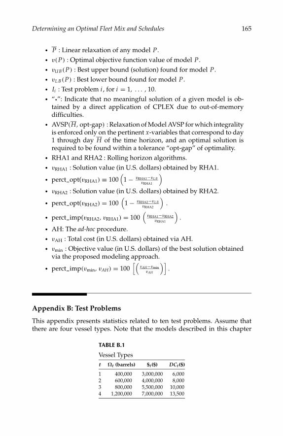
P1: shibu/Vijay

August 12, 2005 10:42 1914 1914˙C006


• P : Linear relaxation of any model P .• v(P) : Optimal objective function value of model P .• vU B(P) : Best upper bound (solution) found for model P .• vL B(P) : Best lower bound found for model P .• Ii : Test problem i , for i = 1, . . . , 10.

• “•”: Indicate that no meaningful solution of a given model is ob-tained by a direct application of CPLEX due to out-of-memorydifficulties.

• AVSP(H, opt-gap) : Relaxation of Model AVSP for which integralityis enforced only on the pertinent x-variables that correspond to day1 through day H of the time horizon, and an optimal solution isrequired to be found within a tolerance “opt-gap” of optimality.

• RHA1 and RHA2 : Rolling horizon algorithms.• vRHA1 : Solution value (in U.S. dollars) obtained by RHA1.

• perct_opt(vRHA1) ≡ 100(

1 − vRHA1−vL BvRHA1

)• vRHA2 : Solution value (in U.S. dollars) obtained by RHA2.

• perct_opt(vRHA2) = 100(

1 − vRHA2−vL BvRHA2

).

• perct_imp(vRHA2, vRHA1) = 100(

vRHA1−vRHA2vRHA1

).

• AH: The ad-hoc procedure.• vAH : Total cost (in U.S. dollars) obtained via AH.• vmin : Objective value (in U.S. dollars) of the best solution obtained

via the proposed modeling approach.

• perct_imp(vmin, vAH) = 100[(

vAH−vminvAH

)].

Appendix B: Test Problems

This appendix presents statistics related to ten test problems. Assume thatthere are four vessel types. Note that the models described in this chapter

TABLE B.1

Vessel Typest Ωt (barrels) $t($) DCt($)

1 400,000 3,000,000 6,0002 600,000 4,000,000 8,0003 800,000 5,500,000 10,0004 1,200,000 7,000,000 13,500

P1: shibu/Vijay

August 12, 2005 10:42 1914 1914˙C006


TABLE B.2

Test ProblemsT (vessel (O1, O2, O3, O4) (CH1, CH2, CH3, CH4) (T1, T2, T3, T4)

Ii H (days) types) (vessels) (vessels) (days) w (barrels)

I1 30 1 (4,0,0,0) (5,0,0,0) (10,0,0,0) 4,000,000I2 60 1 (2,0,0,0) (2,0,0,0) (10,0,0,0) 7,000,000I3 60 2 (2,3,0,0) (2,7,0,0) (10,20,0,0) 7,000,000I4 90 2 (2,2,0,0) (2,3,0,0) (10,20,0,0) 7,000,000I5 120 2 (3,4,0,0) (8,7,0,0) (20,30,0,0) 7,000,000I6 120 4 (1,1,1,1) (3,4,2,6) (20,30,40,50) 7,000,000I7 150 3 (2,5,2,0) (1,5,2,0) (20,30,40,0) 4,000,000I8 180 3 (5,1,6,0) (2,7,9,0) (20,30,40,0) 7,000,000I9 210 4 (4,2,1,4) (3,2,1,4) (20,30,40,50) 7,000,000I10 240 4 (5,2,2,2) (1,2,2,6) (30,40,50,60) 7,000,000

consider a single source-destination operation. We assume that the dailyconsumption rate for a given destination is the same for the duration of agiven time-horizon (denoted by R1), and that the daily operational costs ofvessels of a given type are also the same. The Type I penalty is fixed at $3and the Type II penalty is fixed at $500. Specific details for the test problemsare presented in Table B.1 and Table B.2, where Table B.2 describes our setof ten test problems. Note that R1 = 150, 000, SL1 = 2, 250, 000, SL2 =10, 000, 000, and A1 = A2 = 1, 000, 000 for all the test problems. Also, notethat Ti = 0 indicates that no vessels of type i are involved in the operation.

P1: shibu/Vijay

August 12, 2005 11:0 1914 1914˙C007

7Determining an Optimal Fleet Mixand Schedules: Part II — Multiple Sourcesand Destinations, and the Option of LeasingTransshipment Depots

Hanif D. Sherali and Salem M. Al-Yakoob

CONTENTS

7.1 Introduction . . . . . . . . . . . . . . . . . . . . . . . . . . . . . . . 1687.1.1 Problem Statement . . . . . . . . . . . . . . . . . . . . . . . 1687.1.2 Related Research . . . . . . . . . . . . . . . . . . . . . . . . 168

7.2 Problem Description . . . . . . . . . . . . . . . . . . . . . . . . . . 1707.2.1 Demand Structure . . . . . . . . . . . . . . . . . . . . . . . 1707.2.2 Problem Notation . . . . . . . . . . . . . . . . . . . . . . . . 1707.2.3 Penalty Representations . . . . . . . . . . . . . . . . . . . . 173

7.3 Model Formulation . . . . . . . . . . . . . . . . . . . . . . . . . . . 1747.3.1 A Mixed-Integer Programming Model . . . . . . . . . . . . 1747.3.2 Objective Function . . . . . . . . . . . . . . . . . . . . . . . 1777.3.3 Constraints . . . . . . . . . . . . . . . . . . . . . . . . . . . 177

7.4 An Aggregated Reformulation for Model VSPand Related Issues . . . . . . . . . . . . . . . . . . . . . . . . . . . 1787.4.1 Formulation of Model AVSP . . . . . . . . . . . . . . . . . . 1787.4.2 Objective Function and Constraints . . . . . . . . . . . . . 181

7.5 Solution Algorithms and Computational Results . . . . . . . . . . 1827.5.1 A Rolling Horizon Algorithm for Model AVSP . . . . . . . 1827.5.2 Usefulness of the Proposed Modeling Approach . . . . . . 185

7.6 Summary, Conclusions, and Future Research . . . . . . . . . . . . 185Acknowledgments . . . . . . . . . . . . . . . . . . . . . . . . . . . . . . 186References . . . . . . . . . . . . . . . . . . . . . . . . . . . . . . . . . . . 187

167

P1: shibu/Vijay

August 12, 2005 11:0 1914 1914˙C007


7.1 Introduction

Scheduling the shipment of products to destinations is a challenging problemfaced by many organizations that are interested in improving the efficiencyof their transportation systems due to the high cost associated with opera-tional and penalty costs. Efficient transportation systems have the potentialfor enormous savings. For example, in the oil industry, a typical vessel ina fleet of oil tankers usually costs millions of U.S. dollars, and the daily op-erational costs of an oil tanker amounts to tens of thousands of U.S. dollars.Furthermore, considerable penalties are levied for either shortages in fulfillingcustomer demands, or requiring customers to carry higher than desired levelsof inventory during certain periods. Hence, a formal modeling approach thatcompromises among these different cost components in an effective mannerbecomes imperative.

7.1.1 Problem Statement

Without loss of generality, we assume that the product to be transported iscrude oil and that the transporting vessels are oil tankers. Accordingly, theterms “crude oil” and “product” will be used interchangeably. Hence, sup-pose that an organization is concerned with transporting a product from dif-ferent source points to customers located at various destinations. The sourcepoints might represent refineries or storage facilities either owned or leasedby the organization. There also exist certain specified delivery time-windowsfor the product from the sources to the destinations that are governed by anumber of factors. These factors include the availability of the product at thesources, storage capacities at the destination facilities, rates of consumptionof the product at the destinations, penalties imposed by customers due tounacceptable storage levels, routes available for transportation, vessels avail-able for transportation, transshipment depots available for leasing, and con-tracted constraints agreed upon between the organization and the respectivecustomers. The fleet of vessels utilized by the organization may be composedof self-owned vessels, chartered vessels, or a mix of both.

The leasing of transshipment depots is a strategic decision that is open tothe organization in seeking an overall efficient and cost effective solution.The organization aims to satisfy customer demands for the product basedon agreed-upon contracts at a minimum total cost that is comprised of theoperational costs of the vessels, chartering expenses, penalties associated withviolating certain storage levels, and the cost of leasing storage facilities.

7.1.2 Related Research

This work is an extension to the work of the authors in [6] and [7]. In [6] the au-thors investigated a problem concerned with the scheduling of oil tankers toship various products from one source to different destinations. The demand

P1: shibu/Vijay

August 12, 2005 11:0 1914 1914˙C007


structures that were investigated were determined by the total demand foreach product at each destination, along with the respective subdemands thathave to be satisfied within specified time intervals. It was assumed that somevessels can carry more than one product. In the previous chapter, the au-thors considered a vessel scheduling problem to transport a product from asingle source to a single destination in which the demand for the productis governed by the consumption rates at the destination, with an allowancefor over- or under-shipments, subject to appropriate penalties. Two mixed-integer programming models were developed for this problem: a full-scalerepresentation that incorporates all the detailed features of the problem, andan aggregate model that suppresses the individual identities of the vessels ofeach type, while incorporating this aspect later when prescribing the actualconsignment decisions.

The problem addressed here is similar to that investigated in [7], with theexception that we now accommodate multiple sources and destinations andmoreover, we incorporate the consideration that the organization can leasetemporary transshipment storage facilities having known locations. Note thatby leasing suitable transshipment depots, a cost savings could be realized bystocking the shipments closer to the destinations during slack periods for useduring periods of higher demand, while using fewer vessels, and in particu-lar, avoiding the high costs associated with chartering vessels. Incorporatingmultiple sources and destinations, along with the option of leasing trans-shipment storage facilities in the problem, necessitates novel modeling andalgorithmic considerations in order to derive good quality strategic decisionswith a reasonable computational effort.

In general, vessel routing and scheduling problems can be partitioned intofour categories (see, for example, Al-Yakoob [1] and Christiansen [2]): a) liner,b) tramp, c) industrial, and d) other related models. The bulk of the watertransportation routing and scheduling models deal with the transport anddelivery of cargo. Significantly fewer models have been developed to tacklevessel routing and scheduling problems in the context of passengers. Thisis a consequence of the fact that most vessels transport cargo around theworld, whereas passengers mainly travel by air or land. Similar to the vesselscheduling problems that are investigated in [6] and [7], the problem thatis considered here falls into the fourth category mentioned above. For fur-ther details on vessel scheduling and related models, the reader may refer toAl-Yakoob [1], Christiansen [2], Perakis [3], and Ronen [4, 5], as well as to themore detailed literature review given in Part I of this study [7].

The remainder of this chapter is organized as follows. The next section pro-vides a description of the problem, and Section 7.3 presents a mixed-integerprogramming model for the problem. Due to the immense size of this modelfor most practical problem instances, Section 7.4 proposes an aggregate re-formulation of the problem. Rolling horizon heuristics along with relatedcomputational results based on a set of test instances representing variousoperational scenarios are presented in Section 7.5. Section 7.6 provides resultspertaining to potential enhancements that can be attained via the leasing of

P1: shibu/Vijay

August 12, 2005 11:0 1914 1914˙C007


transshipment depots, and Section 7.7 concludes this chapter with a summary,future research, and recommendations pertaining to implementation.

7.2 Problem Description

As mentioned earlier, the problem considered here is an extension to thework of the authors in [7]. Accordingly, the demand structure, consump-tion rates, and penalty representation considered in this part are similar tothose used in [7]. These are briefly described below for the sake of complete-ness and ease in presentation. Pertinent notation related to the present workis also introduced in this section. For the sake of reader’s convenience, aglossary of notation (sequenced in the order of appearance) is provided inappendix A.

7.2.1 Demand Structure

The demand structure for the problem is influenced by the following factors:a) the storage capacities at client destinations; b) initial levels of storage atdestinations; c) the rates of consumption at client storage facilities; and d)other customer-specific requirements. The rate of consumption of the productmight not be fixed throughout the entire time horizon. The storage level atany client facility is desired to lie between some minimum and maximumallowable limits on any given day of the time horizon. Some customers imposepenalties when the storage level on a given day falls below the minimumdesired level or exceeds the maximum specified level. The latter maximumlevel might be the storage capacity of the facility, and exceeding this capacitywould require resorting to extra temporary storage facilities, thereby resultingin additional cost penalties. More specific details on the characterization ofthe demand structure are prescribed below.

7.2.2 Problem Notation

Contracts between the transporting company and clients are signed sequen-tially over time and accordingly, scheduling decisions are updated every timea new contract is signed. Note that each contract specifies a time horizonalong with required storage levels to fulfill demand. A time horizon associ-ated with a contract is also referred to as a “contract horizon”. Let CTaa

hh,HHdenote a contract that is signed on day aa having a time horizon given byhh, . . . , HH. Suppose that scheduling decisions need to be made at timeaa to fulfill demand requirements for this contract as well as a set of previ-ously signed contracts, say γ of them, that have not been fulfilled by time aa.Let CThh1,HH1 , . . . , CThhγ ,HHγ

denote these previously signed contracts havingtime horizons given by hh1, . . . , HH1 , . . . , hhγ , . . . , HHγ , respectively.

P1: shibu/Vijay

August 12, 2005 11:0 1914 1914˙C007


Note that for i = 1, . . . , γ, HHi > aa. Let AA = maxHH1, HH2, . . . , HHγ ,HH.Then the collective time horizon for the contracts CThh1,HH1 , . . . ,CThhγ ,HHγ

,and CTaa

hh,HH is given by aa, . . . , AA. For the sake of simplicity, we leth = 1, . . . , H index the days of the collective time horizon, which will hence-forth be referred to as the “time horizon.”

Let t = 1, . . . , T denote the types of vessels in the company’s fleet, wheret represents the capacity of a vessel of Type t. For each t = 1, . . . , T , letn = 1, . . . , Mt index the vessels of Type t, and let Ot and CHt = Mt − Ot

respectively denote the number of company-owned vessels and the numberof available vessels of this type that can be possibly chartered. The company-owned vessels are indexed by n = 1, . . . , Ot while the chartered vessels areindexed by n = Ot + 1, . . . , Ot + CHt ≡ Mt. The actual numbers of vesselsof each type that are chartered are effectively determined by the schedulesprescribed by the model. Note that two vessels of the same type might bechartered at different prices. Accordingly, let $t,n be the cost (in U.S. dollars)of chartering a vessel n of type t, for n = Ot + 1, . . . , Ot + CHt, and for eacht = 1, . . . , T . A vessel may be chartered for the entire duration of the timehorizon or for only a specified subset of it, depending on its availability. Thechartering cost given by $t,n is incurred as a fixed-cost whenever the vesselis chartered during the time horizon, regardless of its usage during this timeinterval. This stems from the fact that the chartered vessels will be madeavailable to the (leased-to) company (in our case, KPC) essentially over thehorizon, and the (leased-to) company is free to make any related dispatchingdecisions during this period. Let UTt,n be the maximum number of daysvessel n of type t can be used during the time horizon. This time restrictionis typically needed for maintenance purposes.

Let f = 1, . . . , F denote the storage facilities that are available for leasingover the duration of the contract horizon. Each storage facility is character-ized by its location, capacity, and leasing expenses. For f = 1, . . . , F , let C f

denote the capacity of storage facility f and let $$ f be the cost (in U.S. dollars)of leasing a storage facility f for the duration of the contract horizon. A stor-age facility can effectively be either a source or a destination for a given vesseltrip, based on whether the vessel happens to be respectively loading or un-loading at the storage facility. Let s = 1, . . . , S+ F denote the entire collectionof sources comprised of the company’s sources and the storage facilities thatare available for leasing. The company’s sources are indexed by s = 1, . . . , S,while s = S + 1, . . . , S + F respectively correspond to the storage facilitiesf = 1, . . . , F . Let Qs be the maximum daily permitted amount that can beshipped from source s to any destination. This might represent a production ora storage capacity restriction. Likewise, let d = 1, . . . , D+ F denote the desti-nations (client storage facilities or storage facilities available for leasing). Theclient destinations are indexed by d = 1, . . . , D, while d = D + 1, . . . , D+ Frespectively correspond to the storage facilities f = 1, . . . , F.

Let LEGh,t,n,s1,d,s2 represent a leg for vessel n of type t leaving source s1toward destination d on day h, and then returning to source s2. Let Tt,s1,d,s2

represent the time required to complete LEGh,t,n,s1,d,s2 , which includes the time

P1: shibu/Vijay

August 12, 2005 11:0 1914 1914˙C007


required to load the vessel of type t at source s1, the time this vessel takes totravel to destination d , the unloading time at destination d, and then the timeneeded to travel from destination d to source s2. We assume that there is aunique prescribed route from source s1 to destination d, and likewise, fromdestination d to source s2. Let Tt,s1,d,s2 = T1,t,s1,d,s2 + T2,t,s1,d,s2 , where T1,t,s1,d,s2 isthe time required to load a vessel of type t at source s1 plus the travel time todestination d , and T2,t,s1,d,s2 is the time required to unload at destination d plusthe travel time from destination d to source s2. Vessels of the same type areassumed to have equal values of Tt,s1,d,s2 (and their splits), and this durationis also assumed to be independent of h; i.e., Tt,s1,d,s2 is independent of theday the leg starts (weather effects are neglected). Let DCt,n denote the dailyoperational cost of vessel n of type t. Let Ct,n,s1,d,s2 = Tt,s1,d,s2 (DCt,n), whichis the cost associated with LEGh,t,n,s1,d,s2 . Note that this cost is independent ofthe day the trip starts.

Next, let us define the following sets to identify permissible shipment rout-ing itineraries:

I1 = (s1, d, s2) : where s1 ∈ 1, . . . , S, d ∈ 1, . . . , D, ands2 ∈ 1, . . . , S + F ,

I2 = (s1, d, s2) : where s1 ∈ 1, . . . , S, d ∈ D + 1, . . . , D + F , ands2 ∈ 1, . . . , S, and

I3 = (s1, d, s2) : where s1 ∈ S + 1, . . . , S + F , d ∈ 1, . . . , D, ands2 ∈ 1, . . . , S + F

Note that I1 represents trips initiated from any of the company sourcess1 ∈ 1, . . . , S, headed to a client storage facility d ∈ 1, . . . , D, and then re-turning to a company source or to a leased storage facility s2 ∈ 1, . . . , S + F .I2 represents trips initiated from any of the company sources s1 ∈ 1, . . . , S,headed to one of the leased storage facilities d ∈ D + 1, . . . , D + F , and thenreturning to a company source s2 ∈ 1, . . . , S. I3 represents trips initiatedfrom any of the leased storage facilities s1 ∈ S + 1, . . . , S + F , headed to aclient storage facility d ∈ 1, . . . , D, and then returning to a company sourceor to one of the leased storage facilities s2 ∈ 1, . . . , S + F . Observe that suc-cessive trips between one leased facility and another is disallowed. Hence,I = I1 ∪ I2 ∪ I3 represents all types of permitted trips in the operation.

For d ∈ 1, . . . , D + F , let wd denote the storage level at either destinationd if d ∈ 1, . . . , D, or transshipment depot (d − D) if d ∈ D + 1, . . . , D + F ,at the beginning of the time horizon, i.e., on the first day of the time horizon.Let SL1,d and SL2,d denote the minimum and maximum desired levels, re-spectively, at the storage facility of destination d. Some customers may allowthe storage level to go below or to exceed SL1,d and SL2,d , respectively; how-ever, with a penalty based on the corresponding shortage or excess quantities.Let πd denote the daily penalty for each shortage or excess unit at destinationd. This penalizes shortages and excess quantities at destination d with respectto the desired levels SL1,d and SL2,d , to the extent given by A1,d and A2,d , re-spectively. Let b1,d = SL1,d − A1,d and b2,d = SL2,d + A2,d . Storage levels falling

P1: shibu/Vijay

August 12, 2005 11:0 1914 1914˙C007


below b1,d or in excess of b2,d (up to a sufficiently large upper bound SUBd),while permitted, are highly undesirable, and incur a significantly greaterpenalty λd > πd per unit, at each destination d.

Let Rj,d denote the expected consumption at destination d on day j , forj ∈ 1, . . . , H. Usually, at most two distinct daily consumption rates exist ata given destination. The different daily consumptions arise from the possibleseasonal changes during the horizon, as well as some client-specific consider-ations. Let TCh,d be the total consumption at destination d during the interval1, . . . , h, which is given by TCh,d = h

j=1 Rj,d .

7.2.3 Penalty Representations

Penalties are computed on a daily basis and depend on the storage levels atthe customers’ facilities. These penalties are similar to those introduced in partI, and are extended to address multiple destinations. Let Sh,d be the storagelevel at destination d on day h. Define Type I and Type II penalty functionsas follows.

Type I penalty:

PI (Sh,d) = πd maximum0, (SL1,d − Sh,d), (Sh,d − SL2,d) if Sh,d ∈ [b1,d , b2,d],

and

Type II penalty:

PII(Sh,d) =

πd A1,d + λd (b1,d − Sh,d) if Sh,d ∈ (0, b1,d),

πd A2,d + λd (Sh,d − b2,d) if Sh,d ∈ (b2,d , SUBd),

where πd and λd > πd are as defined above. Note that if Sh,d ∈ [SL1,d , SL2,d ],then the storage level at destination d lies within the desired bounds and nopenalty is induced. If Sh,d ∈ [b1,d , SL1,d) ∪ (SL2,d , b2,d ], then a penalty is in-curred based on the respective shortage or excess quantity at destination d.On the other hand, if Sh,d ∈ [0, b1,d)∪ (b2,d , SUBd ], then a sufficiently large ad-ditional penalty rate is imposed continuously beyond that of PI (.) to indicatethe undesirabity of such a storage level at destination d on any given day ofthe time horizon.

PROPOSITION 7.1Let

Sh,d = S1,h,d − S2,h,d − S3,h,d + S4,h,d + S5,h,d , (7.1)

where

SL1,d ≤ S1,h,d ≤ SL2,d , 0 ≤ S2,h,d ≤ A1,d , 0 ≤ S3,h,d ≤ b1,d ,

0 ≤ S4,h,d ≤ A2,d , and 0 ≤ S5,h ≤ (SUBd − b2,d). (7.2)

Define P(Sh,d) : [0, SUBd ] → [0, ∞) as the linear penalty function.

P1: shibu/Vijay

August 12, 2005 11:0 1914 1914˙C007


P(Sh,d) = πd(S2,h,d + S4,h,d)+λd(S3,h,d + S5,h,d). Then any minimization objectiveformulation that incorporates the term P(Sh,d) defined above along with (7.1) and(7.2) will automatically enforce the sum of the Type I and Type II penalties PI (Sh,d)+PI I (Sh,d).

PROOF The proof is similar to that of Proposition 7.1 in part I for the caseof a single source-destination operation.

7.3 Model Formulation

7.3.1 A Mixed-Integer Programming Model

In order to formulate the problem described in the foregoing section, wedefine the following sets of binary decision variables. Let

Xh,t,n,s1,d,s2 =

1 if LEGh,t,n,s1,d,s2 is selected,

0 otherwise.

Since a vessel cannot be dispatched from source s on day h unless it isavailable on this day, another set of binary variables is defined as follows:

Yh,t,n,s =

1 if vessel n of type t is available at source s on day h,

0 otherwise.

Finally, in order to represent the chartering decisions and the storage leasingdecisions, let

Zt,n =

1 if vessel n ∈ Ot + 1, . . . , Ot + CHt of type t is selected forchartering during the time horizon,

0 otherwise,

and

Wf =

1 if storage facility f is leased for the duration of the time horizon,

0 otherwise.

Note that several of the above defined binary decision variables are a prioriknown to be inadmissible, or effectively, zero. Naturally, whenever Yh,t,n,s1 =0, this implies that the corresponding variables Xh,t,n,s1,d,s2 = 0 ∀ (d, s2).

Examples of such zero variables are specified below.

(A) If (s1, d, s2) /∈ I then this implies that LEGh,t,n,s1,d,s2 is not permittedin the operation ∀ h, t, n. Accordingly, Xh,t,n,s1,d,s2 ≡ 0 ∀ h, t, n, s1, d,s2 such that (s1, d, s2) /∈ I .

P1: shibu/Vijay

August 12, 2005 11:0 1914 1914˙C007


(B) Xh,t,n,s1,d,s2 ≡ 0 ∀ h, n if source s1, or destination d, or source s2, doesnot admit vessels of type t. This occurs if a source or a destinationcannot admit a vessel due to its size or specifications, as in thecase of super-tankers that cannot be admitted into certain source ordestination ports.

(C) A vessel n of type t may not be available for any new consignmentsduring some subset [h1, h2] of the time horizon. Such a situationoccurs if the company needs to perform a scheduled maintenanceon a vessel during some specified days of the time horizon providedthe vessel is in port any time during that duration. This informationcan be incorporated into the model by letting Yh,t,n,s ≡ 0 ∀ h ∈h1, . . . , h2 and ∀ s. Note that if a vessel n of type t is required tobe inactive during [h1, h2], we can set Xh,t,n,s1,d,s2 = 0 ∀ (s1, d, s2) ∈I and ∀h such that [h, h + Tt,s1,d,s2 ] ∩ [h1, h2] = ∅.

(D) The present demand contract might have been signed during a previ-ous contract horizon. In this case, certain decisions for the previouscontract might have committed some self-owned vessels over peri-ods concurrent with the present contract horizon. Therefore, propersets of the X and Y variables should be defined to be zero to indicatethe unavailability of vessels during the present contract horizon.Moreover, whenever a vessel n of type t becomes available for thefirst time on day h in the horizon at source s, we fix Yh,t,n,s = 1, andlet Yh,t,n,s1 = 0 ∀ s1 = s, and Yh1,t,n,s1 = 0 ∀h1 ∈ 1, . . . , (h − 1) andfor all s1.

We will let φX and φY denote the sets of X and Y variables, respectively, thatare restricted to be fixed at specified binary values by virtue of such considera-tions. The prescribed vessel scheduling problem can now be stated as follows.(All indices are assumed to take on only their respective relevant values.)

VSP:

Minimize∑

h

∑t

∑n

∑s1

∑d

∑s2

Ct,n,s1,d,s2 Xh,t,n,s1,d,s2

+∑

h

∑d

πd [S2,h,d + S4,h,d ] +∑

h

∑d

λ[S3,h,d + S5,h,d ]

+∑

t

Mt∑n=Ot+1

$t,n Zt,n +∑

f

$$ f Wf ,

subject to

(C1) Sh,d = wd +∑

t

∑n

∑s1

∑s2

∑h:

h+T1,t,s1 ,d,s2∈1, ... ,h

t Xh,t,n,s1,d,s2− TCh,d ,

∀ h and d ∈ 1, . . . , D,

P1: shibu/Vijay

August 12, 2005 11:0 1914 1914˙C007


(C2) Sh,d = S1,h,d − S2,h,d − S3,h,d + S4,h,d + S5,h,d ,

∀ h and d ∈ 1, . . . , D,

(C3) Lh, f = wD+ f +∑

t

∑n

S∑s1=1

S∑s2=1

∑h:

(h+T1,s1 , D+ f ,s2)∈1, ... ,h

t Xh,t,n,s1, D+ f ,s2

−∑

t

∑n

D∑d=1

∑s2

∑h:

h∈1, ... ,h

t Xh,t,n, S+ f ,d,s2, ∀ h, f ,

(C4) Yh,t,n,s = Yh−1,t,n,s −∑

d

∑s2

Xh−1,t,n,s,d,s2+∑

s1

∑d

∑h:

h+Tt,s1 ,d,s=h

Xh,t,n,s1,d,s ,

∀ h ≥ 2, t, n, s,

(C5)∑

d

∑s2

Xh,t,n,s,d,s2≤ Yh,t,n,s , ∀ h, t, n, s,

(C6)∑

s

Yh,t,n,s ≤ Zt,n, ∀ h, t, n ∈ Ot + 1, . . . , Ot + CHt,

(C7)∑

t

∑n

∑d

∑s1

t Xh,t,n,s,d,s1≤ Qs, ∀ h and s ∈ 1, . . . , S,

(C8.1) Yh,t,n, S+ f ≤ Wf , ∀ h, t, n, f ,

(C8.2)∑

s1

D∑d=1

Xh,t,n,s1,d, D+ f ≤ Wf , ∀ h, t, n, f ,

(C9)∑

h

∑s1

∑d

∑s2

Xh,t,n,s1,d,s2Tt,s1,d,s2

≤ UTt,n, ∀ t, n,

(C10) Xh,t,n,s1,d,s2 ∈ 0, 1, ∀ h, t, n, s1, d, s2, if Xh,t,n,s1,d,s2 /∈ φX,

and fixed at zero or one otherwise,

Yh,t,n,s ∈ [0, 1], ∀h, t, n, s, if Yh,t,n,s /∈ φY,

and fixed at zero or one otherwise,

Zt,n ∈ [0, 1], ∀ t, n = Ot + 1, . . . , Ot + CHt,

Wf ∈ [0, 1], ∀ f,

Sh,d ≥ 0, SL1,d ≤ S1,h,d ≤ SL2,d , 0 ≤ S2,h,d ≤ A1,d ,

0 ≤ S3,h,d ≤ b1,d , 0 ≤ S4,h,d ≤ A2,d ,

P1: shibu/Vijay

August 12, 2005 11:0 1914 1914˙C007


and

0 ≤ S5,h,d ≤ (SUBd − b2,d), ∀ h and d ∈ 1, . . . , D,

0 ≤ Lh, f ≤ C f , ∀ h, f

7.3.2 Objective Function

The objective function of the problem seeks to minimize the total cost com-prised of the operational costs of selected legs (both for company-owned andchartered vessels), the penalty costs resulting from shortage or excess levelsat the customer storage facilities (both of Type I and Type II), the charteringexpenses, and the costs for leasing storage facilities.

7.3.3 Constraints

Revisits to destination d = 1, . . . , D are determined by the initial storagelevel (given by wd), the storage capacity (including minimum and maxi-mum desired levels, given respectively by SL1,d and SL2,d), and the dailyrates of consumption Rj,d . Constraint (C1) computes the storage level atdestination d on day h, whereas Constraint (C2) represents Sh,d in terms ofS1,h,d , S2,h,d , S3,h,d , S4,h,d , and S5,h,d as in Proposition 7.1. The Type I and IIpenalties are incurred in the objective function based on this representation asstated in Proposition 7.1. In Constraint (C3), the variable Lh, f represents thestorage level at facility f on day h, being equal to the difference between thetotal quantity delivered to storage facility f by day h and the total quantityshipped from this storage facility f by day h. Note that Sh,d and Lh, f are non-negative continuous variables, and moreover, Lh, f is bounded above by thestorage capacity given by C f , as noted in Constraint (C10).

A vessel n of type t can be dispatched from source s on day h only if itis available at s on that day. This vessel is available at source s on day hif either the vessel was available there on the previous day and it was notdispatched, or this vessel was not available there during the previous day butit arrived on the current day. On the other hand, this vessel is unavailableon day h at source s if it was available there on the previous day and it wasdispatched on that day, or it was unavailable there on the previous day and itdid not arrive on the current day. Constraint (C4) examines the availability ofvessel n of type t at source s on day h by incorporating these cases (assumingthat any trip is at least two days long), and then Constraint (C5) permits thedispatchment of vessels conditioned on this availability. For the charteredvessels n ∈ Ot +1, . . . , Ot +CHt of type t, Constraint (C6) enforces that thisvessel is selected for chartering (Zt,n = 1) if it is required to be made availablefor consignment. Note that once a chartered vessel is made available at somesource, then (C4) accounts for its proper feasible use. Constraint (C7) ensuresthat the total amount of the product that can be shipped from a given sources on a given day h to any destination d does not exceed the daily permittedamount being specified by Qs . Constraint (C8.1) examines if storage facility f

P1: shibu/Vijay

August 12, 2005 11:0 1914 1914˙C007


is leased for the duration of the time horizon in order to permit the availabilityof vessels thereat and Constraint (C8.2) rules out legs that terminate in non-leased storage facilities. Constraint (C9) enforces that any vessel n of type tcan be used for at most UTt,n days during the time horizon. Finally, (C10)

enforces the various bounding and logical constraints.

REMARK 7.1Assume that the Y-variables corresponding to h = 1 are fixed at some binaryvalues. Then Constraint (C4) ensures the integrality of all the other Y-variablesonce the integrality of the X-variables is enforced. This follows from the re-cursive relation in (C4) that defines Yh,t,n,s for h ≥ 2 in terms of Yh−1,t,n,s and asubset of the X-variables. Moreover, the integrality conditions on the Z- andW-variables can also be relaxed. This follows because constraints (C6), (C8.1),and (C8.2) along with the fourth and fifth terms of the objective function willautomatically enforce the integrality of these variables.

7.4 An Aggregated Reformulation for Model VSPand Related Issues

In this section, we derive an aggregated version of Model VSP, denoted byAVSP, which retains the essential operational features of the original prob-lem, while being far more computationally tractable. The aggregate refor-mulation basically disregards the individual vessel identities, and instead,attempts to decide on the number of vessels of each type to be dispatched ona given day to traverse a prescribed trip. This aggregated reformulation is mo-tivated by the overwhelming number of binary variables resulting from theinitial formulation for a typical operational scenario as illustrated in Table 7.1and Table 7.2 of Section 7.5.1.

7.4.1 Formulation of Model AVSP

Let LEGh,t,s1,d,s2 represent a leg for a vessel of type t leaving source s1 todestination d on day h, and then returning to source s2. The average costassociated with this leg is denoted by ch,t,s1,d,s2 , and the time required tocomplete this leg is given by Tt,s1,d,s2 .

Define xh,t,s1,d,s2 as an integer variable that represents the number of ves-sels of type t that traverse LEGh,t,s1,d,s2 . Define yh,t,s to be an integer decisionvariable that represents the maximum number of vessels of type t that areavailable for consignment from source s on day h. As mentioned in the fore-going section, vessels might become available for use at different days ofthe time horizon due to, for example, their involvement in trips from previ-ously signed contracts that will terminate sometime during the current time

P1: shibu/Vijay

August 12, 2005 11:0 1914 1914˙C007


horizon. Hence, we let Oh,t,s be the number of self-owned vessels of type tthat will become available for use for the first time at source s on day h of thetime horizon, and we let CHh,t,s be the number of vessels of type t that willbecome available for chartering for the first time at source s on day h of thetime horizon. Hence, let αh,t,s = Oh,t,s + CHh,t,s . Accordingly, we let zh,t,s bethe integer variable that represents the number of vessels of type t that areactually selected for chartering on day h of the time horizon at source s. Let$h,t denote the average chartering cost of a vessel of type t that will becomeavailable for use for the first time on day h of the time horizon, regardless ofthe source at which it first became available.

Hence, y1,t,s = O1,t,s +z1,t,s . Note that as before, the y-variables will be usedto indicate the supply distribution of vessels during the time horizon, and theactual use of the vessels will be examined via the x-variables.

Let Ah,t,s be a subset of vessels of type t (both self-owned and vessels avail-able for chartering) that will become available for use at source s for the firsttime on day h of the time horizon. Hence, we let Uh,t = sn∈Ah,t,s UTt,n

sαh,t,s, which

gives the average usage allowance for a vessel of type t that will becomeavailable for use for the first time on day h of the time horizon. Accordingly,Ut = h Uh,t gives the average usage allowance for a vessel of type t. Also,let Ot ≡ hs Oh,t,s .

Similar to the index sets φX and φY, we let φx and φy denote the sets ofx- and y-variables, respectively, that are a priori restricted to be zero, or fixedat some known positive integer values.

The formulation AVSP adopts an aggregated viewpoint as exemplified bythe integer decision variables that represent the number of vessels assignedto traverse from the source points to the various destinations over the timehorizon (without any vessel identities), in lieu of using the previous binaryvariables. Accordingly, as we shall see, we can represent the Model VSP morecompactly using this aggregated representation, at the expense of having torelax the individual vessel’s total usage and downtime restrictions (C9) tothe revised representation (AC9), as we no longer specifically account foreach individual vessel’s activity. These relaxed constraints need to be dealtwith separately while implementing the model-based decision. Because of therelatively soft nature of these constraints, this is an acceptable compromisebetween model size and representability.

The aggregated model is now stated as follows, where the W, S, and Lvariables are defined as in Model VSP.

AVSP:

Minimize∑

h

∑t

∑s1

∑d

∑s2

ct,s1,d,s2 xh,t,s1,d,s2

+∑

h

∑d

πd [S2,h,d + S4,h,d ] +∑

h

∑d

λd [S3,h,d + S5,h,d ]

+∑

h

∑t

∑s

$h,tzh,t,s +∑

f

$$ f Wf ,

P1: shibu/Vijay

August 12, 2005 11:0 1914 1914˙C007


subject to

(AC1) Sh,d = wd +∑

t

∑s1

∑s2

∑h:

h+T1,t,s1 ,d,s2 ∈1, ... ,h

t xh,t,s1,d,s2− TCh,d , ∀ h

and d ∈ 1, . . . , D,(AC2) Sh,d = S1,h,d − S2,h,d − S3,h,d + S4,h,d + S5,h,d , ∀ h

and d ∈ 1, . . . , D,

(AC3) Lh, f = wD+ f +∑

t

S∑s1=1

S∑s2=1

∑h:

(h+T1,s1 , D+ f ,s2)∈1, ... ,h

t xh,t,s1, D+ f ,s2

−∑

t

D∑d=1

∑s2

∑h:

h∈1, ... ,h

t xh,t, S+ f ,d,s2, ∀ h, f ,

(AC4) yh,t,s = yh−1,t,s −∑

d

∑s2

xh−1,t,s,d,s2+∑

s1

∑d∑

h:h+Tt,s1 ,d,s=h

xh,t,s1,d,s + Oh,t,s + zh,t,s , ∀ h ≥ 2, t, s

(AC5)∑

d

∑s2

xh,t,s,d,s2≤ yh,t,s , ∀ h, t, s,

(AC6) y1,t,s = O1,t,s + z1,t,s , ∀ t, s,

(AC7)∑

t

∑d

∑s1

txh,, t,s,d,s2≤ Qs, ∀ h and s ∈ 1, . . . , S,

(AC8.1) y1,t, S+ f ≤ (O1,t, S+ f + CH1,t, S+ f )Wf , ∀ t, f ,

(AC8.2) y h,t, S+ f ≤ MtWf , ∀ h ≥ 2, t, f ,

(AC8.3)∑

s1

D∑d=1

xh,t,s1,d, D+ f ≤ Mt Wf , ∀ h, t, f ,

(AC9)∑

h

∑s1

∑d

∑s2

Tt,s1,d,s2xh,t,s1,d,s2

≤ Ut (Ot +∑

h

∑s

zh,t,s), ∀ t,

(AC10) xh,t,s1,d,s2 ∈ 0, 1, . . . , Mt, ∀ h, t, s1, d, s2, if xh,t,s1,d,s2 /∈ φx,

and fixed at some positive integer values otherwise,

0 ≤ yh,t,s ≤ Mt, ∀ h ≥ 2, t, s, if yh,t,s /∈ φy,

P1: shibu/Vijay

August 12, 2005 11:0 1914 1914˙C007


and fixed at some positive integer values otherwise,

0 ≤ zh,t,s ≤ CHh,t,s , and integer valued ∀ h, t, s,

Wf ∈ 0, 1, ∀ f,

Sh,d ≥ 0, SL1,d ≤ S1,h,d ≤ SL2,d , 0 ≤ S2,h,d ≤ A1,d ,

0 ≤ S3,h,d ≤ b1,d , 0 ≤ S4,h,d ≤ A2,d ,

and

0 ≤ S5,h,d ≤ (SUBd − b2,d), ∀ h and d ∈ 1, . . . , D,0 ≤ Lh, f ≤ C f , ∀ h, f.

7.4.2 Objective Function and Constraints

As before, the objective function of Model AVSP represents the total opera-tional costs for both the company owned vessels and the chartered vessels, thepenalties resulting from shortage or excess levels at the customer storage facil-ities, and the cost of leasing storage facilities. Similar to constraints (C1), (C2),and (C3) of Model VSP, the constraints (AC1), (AC2), and (AC3) respectivelyrepresent storage levels at customers’ facilities, decomposed storage levels forpenalty representations, and storage levels at the leased facilities. Constraints(AC4), (AC5), (AC7), and (AC9) are used as representations of constraints (C4),(C5), (AC7), and (C9) respectively, in an aggregated sense. Note that (AC9) isa relaxed version of (C9) where the right-hand-side of (AC9) gives the totalallowable utilization of all the self-owned and chartered vessels. Constraint(AC6) in concert with constraints (AC4) and (AC5) account for the numberof chartered vessels. Restrictions related to the leasing facilities are enforcedvia the W-variables in constraints (AC8.1) to (AC8.3). The right-hand-sides of(AC8.1) to (AC8.3) yield the maximum number of vessels of type t that can bepossibly available at a given leasing storage facility during the pertinent daysof the time horizon. This number equals (O1,t, S+ f + CH1,t, S+ f ) when h = 1,and equals Mt when h ≥ 2, if the particular leasing facility is actually leasedduring the time horizon (Wf = 1), and equals zero otherwise. Note that Con-straint (AC8.3) assures that if a storage facility is not selected, then this facilityis not the termination point of any vessel, because otherwise, such a vesselwould end up idle at this storage facility until the end of the time horizon.Observe that the integrality conditions on the y-variables are relaxed in ModelAVSP for similar reasoning as discussed in Remark 7.1 above.

Having solved Model AVSP, the variable zt ≡ hs zh,t,s at optimality yieldsthe number of vessels of type t to charter, thereby determining the fleet of ves-sels being composed of company-owned and chartered vessels. The leasingof storage facility is determined at optimality by the binary variables Wf for

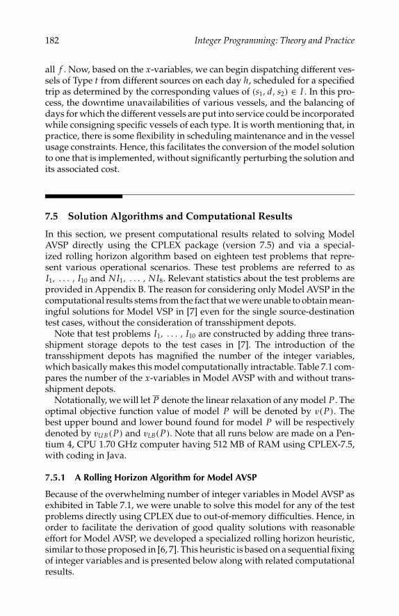
P1: shibu/Vijay

August 12, 2005 11:0 1914 1914˙C007


all f . Now, based on the x-variables, we can begin dispatching different ves-sels of Type t from different sources on each day h, scheduled for a specifiedtrip as determined by the corresponding values of (s1, d, s2) ∈ I . In this pro-cess, the downtime unavailabilities of various vessels, and the balancing ofdays for which the different vessels are put into service could be incorporatedwhile consigning specific vessels of each type. It is worth mentioning that, inpractice, there is some flexibility in scheduling maintenance and in the vesselusage constraints. Hence, this facilitates the conversion of the model solutionto one that is implemented, without significantly perturbing the solution andits associated cost.

7.5 Solution Algorithms and Computational Results

In this section, we present computational results related to solving ModelAVSP directly using the CPLEX package (version 7.5) and via a special-ized rolling horizon algorithm based on eighteen test problems that repre-sent various operational scenarios. These test problems are referred to asI1, . . . , I10 and NI1, . . . , NI8. Relevant statistics about the test problems areprovided in Appendix B. The reason for considering only Model AVSP in thecomputational results stems from the fact that we were unable to obtain mean-ingful solutions for Model VSP in [7] even for the single source-destinationtest cases, without the consideration of transshipment depots.

Note that test problems I1, . . . , I10 are constructed by adding three trans-shipment storage depots to the test cases in [7]. The introduction of thetransshipment depots has magnified the number of the integer variables,which basically makes this model computationally intractable. Table 7.1 com-pares the number of the x-variables in Model AVSP with and without trans-shipment depots.

Notationally, we will let P denote the linear relaxation of any model P . Theoptimal objective function value of model P will be denoted by v(P). Thebest upper bound and lower bound found for model P will be respectivelydenoted by vU B(P) and vLB(P). Note that all runs below are made on a Pen-tium 4, CPU 1.70 GHz computer having 512 MB of RAM using CPLEX-7.5,with coding in Java.

7.5.1 A Rolling Horizon Algorithm for Model AVSP

Because of the overwhelming number of integer variables in Model AVSP asexhibited in Table 7.1, we were unable to solve this model for any of the testproblems directly using CPLEX due to out-of-memory difficulties. Hence, inorder to facilitate the derivation of good quality solutions with reasonableeffort for Model AVSP, we developed a specialized rolling horizon heuristic,similar to those proposed in [6, 7]. This heuristic is based on a sequential fixingof integer variables and is presented below along with related computationalresults.

P1: shibu/Vijay

August 12, 2005 11:0 1914 1914˙C007


In Model AVSP, let the vector x be partitioned as (x1, x2, . . . , xH), wherexh denotes the vector of x−variables associated with the hth day of the timehorizon. Let H1 be the length of the horizon interval for which the correspond-ing x variables are restricted to be integer valued, and the remaining variablesare declared to be continuous. Accordingly, in a rolling-horizon framework,let H2 be the duration of the initial subset of this interval for which the deter-mined decisions are permanently fixed. Let K K = ((H − H1)/H2) + 1 andlet AVSP (H1, H2, opt-gap, k), for k = 1, . . . , K K , denote Model AVSP hav-ing the following characteristics:

(a) xh is enforced to be integer valued for h ≤ H1 + (k − 1)H2, and isrelaxed to be continuous otherwise, ∀ h = 1, . . . , H.

(b) xh for h ≤ (k − 1)H2 is fixed at the values found from the solutionto Model AVSP(H1, H2, opt-gap, (k − 1)).

(c) The optimality gap tolerance for fathoming is set at opt-gap.

The rolling-horizon heuristic RHA then proceeds as follows.

Initialization: Select integers H1 ≤ H, H2 ≤ (H1/2), and initialize k = 1.Let opt-gap be some selected optimality gap criterion. Solve Model AVSP(H1, H2, opt-gap, 1).

Main Step: If k = KK; then terminate the algorithm; the proposed solutionis that obtained from solving Model AVSP (H1, H2, opt-gap, KK). Otherwise,increment k by one and solve the Model AVSP (H1, H2, opt-gap, k). Repeatthe Main Step.

Note that the solution value obtained from the first iteration of the algorithmRHA provides a lower bound for problem AVSP that is at least as high asv(AVSP). Accordingly, we let vLB equal the objective value obtained fromthe first iteration of the algorithm RHA. Table 7.2 reports results obtained

TABLE 7.1

Number of the x-Variables for Model AVSP withand without Transshipment Depots

No Transshipment 3 TransshipmentDepots Depots

TestProblem Total Number of x-Variables

I1 30 570I2 60 1,140I3 120 2,280I4 180 3,420I5 240 4,560I6 480 9,120I7 450 8,550I8 540 10,260I9 840 15,960I10 960 18,240

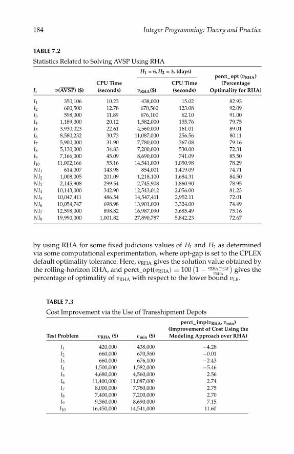
P1: shibu/Vijay

August 12, 2005 11:0 1914 1914˙C007


TABLE 7.2

Statistics Related to Solving AVSP Using RHAH1 = 6, H2 = 3, (days)

perct_opt (vRHA)CPU Time CPU Time (Percentage

Ii v(AVSP) ($) (seconds) vRHA($) (seconds) Optimality for RHA)

I1 350,106 10.23 438,000 15.02 82.93I2 600,500 12.78 670,560 123.08 92.09I3 598,000 11.89 676,100 62.10 91.00I4 1,189,000 20.12 1,582,000 155.76 79.75I5 3,930,023 22.61 4,560,000 161.01 89.01I6 8,580,232 30.73 11,087,000 256.56 80.11I7 5,900,000 31.90 7,780,000 367.08 79.16I8 5,130,000 34.83 7,200,000 530.00 72.31I9 7,166,000 45.09 8,690,000 741.09 85.50I10 11,002,166 55.16 14,541,000 1,050.98 78.29NI1 614,007 143.98 854,001 1,419.09 74.71NI2 1,008,005 201.09 1,218,100 1,684.31 84.50NI3 2,145,908 299.54 2,745,908 1,860.90 78.95NI4 10,143,000 342.90 12,543,012 2,056.00 81.23NI5 10,047,411 486.54 14,547,411 2,952.11 72.01NI6 10,054,747 698.98 13,901,000 3,324.00 74.49NI7 12,598,000 898.82 16,987,090 3,685.49 75.16NI8 19,990,000 1,001.82 27,890,787 5,842.23 72.67

by using RHA for some fixed judicious values of H1 and H2 as determinedvia some computational experimentation, where opt-gap is set to the CPLEXdefault optimality tolerance. Here, vRHA gives the solution value obtained bythe rolling-horizon RHA, and perct_opt(vRHA) ≡ 100

(1 − vRHA−vLB

vRHA

)gives the

percentage of optimality of vRHA with respect to the lower bound vLB.

TABLE 7.3

Cost Improvement via the Use of Transshipment Depotsperct_imp(vRHA, vmin)

(Improvement of Cost Using theTest Problem vRHA ($) vmin ($) Modeling Approach over RHA)

I1 420,000 438,000 −4.28I2 660,000 670,560 −0.01I3 660,000 676,100 −2.43I4 1,500,000 1,582,000 −5.46I5 4,680,000 4,560,000 2.56I6 11,400,000 11,087,000 2.74I7 8,000,000 7,780,000 2.75I8 7,400,000 7,200,000 2.70I9 9,360,000 8,690,000 7.15I10 16,450,000 14,541,000 11.60

P1: shibu/Vijay

August 12, 2005 11:0 1914 1914˙C007


7.5.2 Usefulness of the Proposed Modeling Approach

In [7], we compared the costs of schedules generated via the proposed ap-proach with the cost of schedules generated via an ad-hoc procedure in a casestudy concerning Kuwait Petroleum Corporation (KPC). It was emphasizedthat significant savings can be achieved via the proposed approach in [7].In this section, we examine the potential cost improvement via accommo-dating the consideration of leasing transshipment depots, whereby fewerchartered vessels might need to be acquired. We also emphasize the cost ef-fectiveness of simultaneously examining multiple sources and destinationsinstead of associating specific vessels with designated source-destinationcombinations.

The following table compares costs of schedules obtained from [7], whereno transshipment depots are utilized, with those obtained here, where threetransshipment depots are available for usage. Note that vmin gives the solutionvalue obtained from [7], and hence, perct_imp(vRHA,vmin) = 100

(vmin−vRHA

vmin

)yields the percentage of improvement in total cost when allowing the usageof the transshipment depots.

The use of the transshipment depots improved the total cost for test prob-lems I5 − I10, with a percentage reduction in total cost ranging from 2.56 to11.60. It is worth mentioning that for test problems I1 − I4, we were able tosolve Model AVSP without transshipment depots directly using the CPLEXPackage with the default setting in [7], while we utilized the heuristic RHAto solve this model when incorporating the three transshipment depots. Con-sequently, the advantage of incorporating the three transshipment depots wasnot discernable in test problems I1 − I4.

As depicted in Appendix B, each test problem NIk for k = 1, . . . , 8, com-bines two single source-destination cases to form a new instance that iscomposed of two sources and two destinations. In particular, a test problemNIk that correspond to Ii, j as defined in Appendix B indicates that NIk com-bines test problems Ii and I j . Let vRHA(TP) denote the objective value obtainedfor Model AVSP via algorithm RHA based on test problem TP and define

vi, jRHA = vRHA(Ii ) + vRHA(I j ). Also, let perct_imp(vRHA,vi, j

RHA) = 100(

vi , jRHA

−vRHA

vi, jRHA

).

Observe that vRHA is lower than vi, jRHA for all the test problems NIk for k =

1, . . . , 8, with a percentage reduction in total cost ranging from 2.20 to 19.83.

7.6 Summary, Conclusions, and Future Research

This research is a continuation of the work of the authors in [6] and [7] con-cerning the scheduling of oil tankers. In particular, this work is an extensionof the work in the previous chapter in that we consider multiple sources anddestinations, and the leasing of transshipment depots, which can enhance

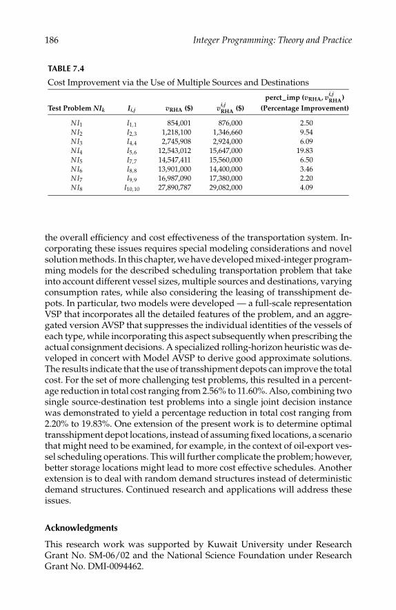
P1: shibu/Vijay

August 12, 2005 11:0 1914 1914˙C007


TABLE 7.4

Cost Improvement via the Use of Multiple Sources and Destinations

perct_imp (vRHA, vi,jRHA)

Test Problem NIk Ii,j vRHA ($) vi,jRHA ($) (Percentage Improvement)

NI1 I1,1 854,001 876,000 2.50NI2 I2,3 1,218,100 1,346,660 9.54NI3 I4,4 2,745,908 2,924,000 6.09NI4 I5,6 12,543,012 15,647,000 19.83NI5 I7,7 14,547,411 15,560,000 6.50NI6 I8,8 13,901,000 14,400,000 3.46NI7 I9,9 16,987,090 17,380,000 2.20NI8 I10,10 27,890,787 29,082,000 4.09

the overall efficiency and cost effectiveness of the transportation system. In-corporating these issues requires special modeling considerations and novelsolution methods. In this chapter, we have developed mixed-integer program-ming models for the described scheduling transportation problem that takeinto account different vessel sizes, multiple sources and destinations, varyingconsumption rates, while also considering the leasing of transshipment de-pots. In particular, two models were developed — a full-scale representationVSP that incorporates all the detailed features of the problem, and an aggre-gated version AVSP that suppresses the individual identities of the vessels ofeach type, while incorporating this aspect subsequently when prescribing theactual consignment decisions. A specialized rolling-horizon heuristic was de-veloped in concert with Model AVSP to derive good approximate solutions.The results indicate that the use of transshipment depots can improve the totalcost. For the set of more challenging test problems, this resulted in a percent-age reduction in total cost ranging from 2.56% to 11.60%. Also, combining twosingle source-destination test problems into a single joint decision instancewas demonstrated to yield a percentage reduction in total cost ranging from2.20% to 19.83%. One extension of the present work is to determine optimaltransshipment depot locations, instead of assuming fixed locations, a scenariothat might need to be examined, for example, in the context of oil-export ves-sel scheduling operations. This will further complicate the problem; however,better storage locations might lead to more cost effective schedules. Anotherextension is to deal with random demand structures instead of deterministicdemand structures. Continued research and applications will address theseissues.

Acknowledgments

This research work was supported by Kuwait University under ResearchGrant No. SM-06/02 and the National Science Foundation under ResearchGrant No. DMI-0094462.

P1: shibu/Vijay

August 12, 2005 11:0 1914 1914˙C007


References

1. Al-Yakoob, S.M., Mixed-integer mathematical programming optimization mod-els and algorithms for an oil tanker routing and scheduling problem, PhD. dis-sertation, Department of Mathematics, Virginia Polytechnic Institute and StateUniversity, Blacksburg, 1997.

2. Christiansen, M., Fagerholt, K., and Ronen, D., Ship routing and scheduling:status and prospective, Transportation Science, 38(1), 1, 2004.

3. Perakis, A.N., Fleet operations optimization and fleet deployment, in The HandBook of Maritime Economics and Business, Grammenos, C.T., Ed., Lloyds of LondonPublications, London, 580, 2002.

4. Ronen, D., Cargo ships routing and scheduling: survey of models and problems,European Journal of Operational Research, 12, 119, 1983.

5. Ronen, D., Ship scheduling: the last decade, European Journal of Operational Re-search, 71, 325, 1993.

6. Sherali, H.D., Al-Yakoob, S.M., and Merza, H., Fleet management models andalgorithms for an oil-tanker routing and scheduling problem. IIE Transactions,31, 395, 1999.

7. Sherali, H.D. and Al-Yakoob, S.M. Determining an optimal fleet mix and sched-ules: Part I—single source and destination. Department of Mathematics andComputer Science, Kuwait University, 2004. (Part II of this sequence is thepresent chapter.)

Appendix A: Glossary of Notation

• CTaahh,HH : A contract that is singed on day aa having a time horizon

given by hh, . . . , HH.• CThh1,HH1 , . . . , CThhγ ,HHγ

: Contracts that are signed prior to Con-tract CTaa

hh,HH having time horizons given by hh1, . . . , HH1, . . . ,hhγ , . . . , HHγ , respectively, where HHi > aa for i = 1, . . . , γ .

• AA = maxHH1, HH2, . . . , HHγ , HH.• aa, . . . , AA : Collective time horizon for the contracts CThh1,HH1 , . . . ,

CThhγ ,HHγ, and CTaa

hh,HH.• H : Number of days in the time horizon.• h = 1, . . . , H : Days of the time horizon.• t = 1, . . . , T : Types of vessels.• t : Capacity (in barrels) of a vessel of type t.• Mt : Total number of vessels of type t.

• M =T∑

t=1Mt.

• Ot : Total number of self-owned vessels of type t.

P1: shibu/Vijay

August 12, 2005 11:0 1914 1914˙C007


• O =T∑

t=1Ot.

• CHt : Total number of vessels of type t that are available forchartering.

• CHt = Mt − Ot.

• CH =T∑

t=1CHt.

• n = 1, . . . , Mt : Vessels of type t.• n = 1, . . . , Ot : Self-owned vessels.• n = Ot + 1, . . . , Ot + CHt ≡ Mt : Vessels of type t that are available

for chartering.• $t,n : Cost (in U.S. dollars) of chartering a vessel n of type t, for

n = Ot + 1, . . . , Ot + CHt ≡ Mt and for each t = 1, . . . , T.

• UTt,n : Maximum number of days that vessel n of type t can be usedduring the time horizon.

• f = 1, . . . , F : Storage facilities that are available for leasing overthe duration of the contract horizon.

• C f : Capacity (in barrels) of storage facility f .• $$ f : Cost (in U.S. dollars) of leasing a storage facility f for the

duration of the contract horizon.• s = 1, . . . , S+ F : Entire collection of sources comprised of the com-

pany’s sources and the storage facilities that are available for leasing.• s = 1, . . . , S : Indices for the company sources.• s = S + 1, . . . , S + F : Source indices for the storage facilities

f = 1, . . . , F .• d = 1, . . . , D + F : Entire collection of destinations (client storage

facilities or storage facilities available for leasing).• d = 1, . . . , D : Indices for the client destinations.• d = D + 1, . . . , D + F : Destination indices corresponding to the

storage facilities f = 1, . . . , F .• LEGh,t,n,s1,d,s2 : A leg for vessel n of type t leaving source s1 to desti-

nation d on day h, and then returning to source s2.• Tt,s1,d,s2 : Time (in days) required to complete LEGh,t,n,s1,d,s2 .• Tt,s1,d,s2 = T1, t, s1, d, s2 + T2, t, s1, d, s2, where T1,t,s1,d,s2 is the time

required to load a vessel of type t at source s1 plus the travel timeto destination d , and T2,t,s1,d,s2 is the time required to unload at des-tination d plus the travel time from destination d to source s2.

• DCt,n : Daily operational cost (in U.S. dollars) of vessel n of type t.• Ct,n,s1,d,s2 = Tt,s1,d,s2 (DCt,n) : Cost (in U.S. dollars) associated with

LEGh,t,n,s1,d,s2 .

P1: shibu/Vijay

August 12, 2005 11:0 1914 1914˙C007


• I1 = (s1, d, s2) : where s1 ∈ 1, . . . , S, d ∈ 1, . . . , D, and s2 ∈1, . . . , S + F .

• I2 = (s1, d, s2) : where s1 ∈ 1, . . . , S, d ∈ D + 1, . . . , D +F , and s2 ∈ 1, . . . , S .

• I3 = (s1, d, s2) : where s1 ∈ S + 1, . . . , S + F , d ∈ 1, . . . , D,and s2 ∈ 1, . . . , S + F .

• I = I1 ∪ I2 ∪ I3.

• wd : Storage level (in barrels) at destination d at the beginning of thetime horizon.

• SL1,d and SL2,d : Minimum and maximum desired levels (in barrels),respectively, at the storage facility of destination d.

• πd : Type I daily penalty (in U.S. dollars) for each shortage or excessunit at destination d .

• A1,d and A2,d : Permitted shortage and excess quantities (in barrels)at destination d with respect to the desired levels SL1,d and SL2,d ,respectively.

• b1,d = SL1,d − A1,d .

• b2,d = SL2,d + A2,d .

• λd : Type II penalty (in U.S. dollars) associated with destination d.• SUBd : A sufficiently large upper bound (in barrels) on the storage

level at destination d .

• TCh,d =h∑

j=1Rj,d .

• Qs : Production capacity (in barrels) at source s ∈ 1, . . . , S.• Sh,d : A continuous variable that represents the storage level at des-

tination d on day h.• PI (Sh,d) = πd maximum

0, (SL1,d − Sh,d), (Sh,d − SL2,d) if Sh,d ∈

[b1,d , b2,d ].

• PII(Sh,d) =

πd A1,d + λd (b1,d − Sh,d) if Sh,d ∈ (0, b1,d),

πd A2,d + λd (Sh,d − b2,d) if Sh,d ∈ (b2,d , SUBd),

• Sh,d = S1,h,d − S2,h,d − S3,h,d + S4,h,d + S5,h,d , whereSL1,d ≤ S1,h,d ≤ SL2,d , 0 ≤ S2,h,d ≤ A1,d ,

0 ≤ S3,h,d ≤ b1,d , 0 ≤ S4,h,d ≤ A2,d , 0 ≤ S5,h ≤ (SUBd − b2,d).

• P(Sh,d) = πd(S2,h,d + S4,h,d) + λd(S3,h,d + S5,h,d).

• Xh,t,n,s1,d,s2 =

1 if LEGh,t,n,s1,d,s2 is selected,

0 otherwise.

• Yh,t,n,s =

1 if vessel n of type t is available at source s on day h,

0 otherwise.

P1: shibu/Vijay

August 12, 2005 11:0 1914 1914˙C007


• Zt,n =

1 if vessel n ∈ Ot + 1, . . . , Ot + CHt of type t is selectedfor chartering during the time horizon,

0 otherwise.

• Wf =

1 if storage facility f is leased for the duration of thetime horizon,

0 otherwise.

• φX and φY : Sets of X and Y variables, respectively, that are restrictedto be fixed at specified binary values.

• LEGh,t,s1,d,s2 : A leg for a vessel of type t leaving source s1 to desti-nation d on day h, and then returning to source s2.

• ct,s1,d,s2 : Average cost (in U.S. dollars) associated with LEGh,t,s1,d,s2 .• xh,t,s1,d,s2 : An integer variable that represents the number of vessels

of type t that traverse LEGh,t,s1,d,s2 .

• yh,t,s : An integer decision variable that represents the maximumnumber of vessels of type t that are available for consignment fromsource s on day h.

• Oh,t,s : Number of self-owned vessels of type t that will become avail-able for use for the first time at source s on day h of the time horizon.

• αh,t,s : Number of vessels of type t that are available (self-owned orthose that would be possibly chartered) for use at source s on dayh of the time horizon.

• CHh,t,s : Number of vessels of type t that will become available forchartering for the first time at source s on day h of the time horizon.

• αh,t,s = Oh,t,s + CHh,t,s .

• zh,t,s : An integer variable that represents the number of vessels oftype t that are actually selected for chartering on day h of the timehorizon at source s.

• $h,t : Average chartering cost (in U.S. dollars) of a vessel of type t thatwill become available for use for the first time on day h of the timehorizon, regardless of the source at which it first became available.

• y1,t,s = O1,t,s + z1,t,s

• Ah,t,s : A subset of vessels of type t (both self-owned and vesselsavailable for chartering) that will become available for use at sources for the first time on day h of the time horizon.

• Uh,t =∑

s

∑UTt,nn∈Ah,t,s∑

sαh,t,s

,

• UTt =∑h

UTh,t.

• Ot =∑h

∑s

Oh,t,s .

• φx and φy : Sets of x- and y-variables, respectively, that are a priorirestricted to be zero, or fixed at some known positive integer values.

P1: shibu/Vijay

August 12, 2005 11:0 1914 1914˙C007


• P : Linear relaxation of any model P .• v(P) : Optimal objective function value of model P .• vUB(P) : Best upper bound (solution) found for model P .• vLB(P) : Best lower bound found for model P .• Ii : Test problem i , for i = 1, . . . , 10.

• NIk : Test problem k, for i = 1, . . . , 8.

• RHA : The rolling horizon algorithm.• vRHA : Solution value obtained by RHA.• perct_opt(vRHA) ≡ 100(1 − vRHA−vLB

vRHA) : Percentage of optimality of

vRHA.

• perct_imp(vRHA, vmin) = 100( vmin−vRHAvmin

) : Percentage of improvementin total cost when allowing the usage of the transshipment depots.

• vRHA(TP) : Objective value obtained for Model AVSP via algorithmRHA based on test problem TP.

• vi, jRHA = vRHA(Ii ) + vRHA(I j ).

• perct_imp(vRHA, vi, jRHA) = 100(

vi, jRHA

−vRHA

vi, jRHA

).

Appendix B: Test Problems

This appendix presents statistics related to eighteen test problems.Assume that there are four vessel types (T = 4) and three transshipment

depots (F = 3). The daily consumption rate for all destinations is assumedto be the same for the duration of the given time horizon, and given byR = 150,000. We also assume that SL1,d = 2, 250,000, SL2,d = 10,000,000, andA1,d = A2,d = 1, 000,000 for all d. The type I and type II penalties are fixed atπd = 3 and λd = 500 for all d . Moreover, we assume that the daily operationalcosts of vessels of a given type are the same, and hence, DCt,n = DCt for n =1, . . . , Mt. Specific details pertaining to the vessel types and transshipmentdepots are presented in the remainder of this appendix.

TABLE B.1

Vessel-Typest Ωt (barrels) $t ($) DCt ($)

1 400,000 $3,000,000 $6,0002 600,000 $4,000,000 $8,0003 800,000 $5,500,000 $10,0004 1,200,000 $7,000,000 $13,500

P1: shibu/Vijay

August 12, 2005 11:0 1914 1914˙C007


TABLE B.2

Transshipment Depotsf Cf (barrels) $$f ($)

1 3,000,000 $1,000,0002 4,000,000 $1,500,0003 5,000,000 $2,000,000

Table B.3 presents ten single source-destination test problems, denoted byI1, . . . , I10. The number of self-owned vessels and the number of vesselsavailable for chartering of type t that are considered in test problem Ii are re-spectively denoted by Oi

t and CHit. Hence, we let Oi

∗ = (Oi1, Oi

2, Oi3, Oi

4) andCHi

∗ = (CHi1, CHi

2, CHi3, CHi

4). Let Ti1,s1,d,s2

, Ti2,s1,d,s2

, and Tis1,d,s2

respectivelydenote the parameters corresponding to T1,s1,d,s2 , T2,s1,d,s2 and Ts1,d,s2 in testproblem Ii . Assume that Ti

1,t,1,1,1 = Ti2,t,1,1,1 = (0.5)Ti

t,1,1,1, Ti1,t,1,1+ f,1 =

Ti2,t,1,1+ f,1 = (0.5)Ti

1,t,1,1,1+ f, Ti1,t,1+ f,1,1+ f = Ti

2,t,1+ f,1,1+ f = (0.5)Ti1,t,1,1,1+ 2 f,

where (1 + f ) is the index for the f th transshipment depot. Hence, all thetravel times for a particular test problem Ii are defined in terms of Ti

t,1,1,1.

Let Ti∗ = (Ti

1,1,1,1, Ti2,1,1,1, Ti

3,1,1,1, Ti4,1,1,1) and let wi represent the initial storage

level associated with test problem Ii . Note that the time required to traveldirectly from a source to a destination is always less than the time requiredto travel from that source to a transshipment depot plus the time requiredto travel from the transshipment depot to the destination. Also, Ti

t,1,1,1 = 0indicates that no vessels of type t are considered in test problem Ii .

Note that the above test problems are those considered in part I, in additionto incorporating three transshipment storage depots. Next, we define a set ofeight test problems, each involving two sources and two destinations. Let(sk , dk) denote the source-destination pair associated with test problemIk , fork = 1, . . . , 10. Let Ii, j for i, j ∈ 1, . . . , 10 denote the test problem thathas the sources si and s j , and the destinations di and d j . For the sake ofconsistency in notation, we let s = 1, 2 respectively index the sources si

and s j , and we let d = 1, 2 respectively index the destinations di and d j .

TABLE B.3

Description of the Test Problems Having a Single Source and DestinationTest Problem Ii H (days) T Oi

∗ CHi∗ Ti

∗ (days) wi (barrels)

I1 30 1 (4,0,0,0) (5,0,0,0) (10,0,0,0) 4,000,000I2 60 1 (2,0,0,0) (2,0,0,0) (10,0,0,0) 7,000,000I3 60 2 (2,3,0,0) (2,7,0,0) (10,20,0,0) 7,000,000I4 90 2 (2,2,0,0) (2,3,0,0) (10,20,0,0) 7,000,000I5 120 2 (3,4,0,0) (8,7,0,0) (20,30,0,0) 7,000,000I6 120 4 (1,1,1,1) (3,4,2,6) (20,30,40,50) 7,000,000I7 150 3 (2,5,2,0) (1,5,2,0) (20,30,40,0) 4,000,000I8 180 3 (5,1,6,0) (2,7,9,0) (20,30,40,0) 7,000,000I9 210 4 (4,2,1,4) (3,2,1,4) (20,30,40,50) 7,000,000I10 240 4 (5,2,2,2) (1,2,2,6) (30,40,50,60) 7,000,000

P1: shibu/Vijay

August 12, 2005 11:0 1914 1914˙C007


TABLE B.4

Description of the Test Problems Having Multiple Sources and DestinationsTest Problem H (days) T O∗ CH ∗

NI1 I1,1 30 1 (8,0,0,0) (10,0,0,0)NI2 I2,3 60 2 (4,3,0,0) (4,7,0,0)NI3 I4,4 90 2 (4,4,0,0) (4,6,0,0)NI4 I5,6 120 4 (4,5,1,1) (11,11,2,6)NI5 I7,7 150 3 (4,10,4,0) (2,10,4,0)NI6 I8,8 180 3 (15,3,18,0) (6,21,27,0)NI7 I9,9 210 4 (12,6,3,12) (9,6,3,12)NI8 I10,10 240 4 (15,6,6,6) (3,6,6,18)

The direct source-destination and destination-source trips that test problemIi, j incorporates are those described by test problems Ii and I j , in addition tofour more trips, two that traverse from si to d j , and two others that traversefrom s j to di . Let Ti, j

t,s1,d,s2denote the travel time associated with LEGh,t,s1,d,s2

in test problemIi, j .Note that for the sake of simplicity and ease in comparison between costs

associated with test problem Ii, j , and the summation of costs associated withits component test problems Ii and I j , we make the following assumptions:

a) We only combine test problems that have the same time horizon.

b) If (s1, d, s2) is a feasible leg in test problem Ii , then Ti, jt,s1,d,s2

= Tit,s1,d,s2

,Ti, j

1,t,s1,d,s2= Ti

1,t,s1,d,s2, and Ti, j

2,t,s1,d,s2= Ti

2,t,s1,d,s2. In a similar fashion,

if (s1, d, s2) is a feasible leg in test problem I j , then Ti, jt,s1,d,s2

= T jt,s1,d,s2

,Ti, j

1,t,s1,d,s2= T j

1,t,s1,d,s2, and Ti, j

2,t,s1,d,s2= T j

2,t,s1,d,s2.

c) The travel times for trips that do not belong to either test problem Ii

or I j (i.e., the trips that involve s1 and d2, or s2 and d1), are given asfollows: Ti, j

1,t,1,2,1 = Ti, j2,t,1,2,1 = Ti, j

1,t,1,1,1 + 2 and Ti, j1,t,2,1,2 = Ti, j

2,t,2,1,2 =Ti, j

1,t,2,2,2 + 3.

d) The total number of self owned and chartered vessels of type t thatare considered in test problem Ii, j are respectively given by Oi, j

t =Oi

t + O jt and CHi, j

t = CHit +CH j

t , for t ∈ 1, . . . , 4. Accordingly, wedenote Oi, j

∗ = (Oi1 + O j

1 , Oi2 + O j

2 , Oi3 + O j

3 , Oi4 + O j

4 ) and CHi, j∗ =

(CHi1 + CH j

1 , CHi2 + CH j

2 , CHi3 + CH j

3 , CHi4 + CH j

4).

P1: shibu/Vijay

August 12, 2005 11:0 1914 1914˙C007

P1: shibu/Vijay

August 8, 2005 15:8 1914 1914˙C008

8An Integer Programming Model forthe Optimization of Data Cycle Maps

David Panton, Maria John, and Andrew Mason

CONTENTS

8.1 Introduction . . . . . . . . . . . . . . . . . . . . . . . . . . . . . . . 1958.2 The Data Cycle Map Structure . . . . . . . . . . . . . . . . . . . . . 1978.3 Designing a Minor Frame . . . . . . . . . . . . . . . . . . . . . . . 1998.4 Optimization Models . . . . . . . . . . . . . . . . . . . . . . . . . . 207

8.4.1 Generalized Set Packing Model . . . . . . . . . . . . . . . . 2078.5 Strengthening the Set Packing Integer Programming Model . . . 209

8.5.1 Pairwise Slot Constraints . . . . . . . . . . . . . . . . . . . 2108.5.2 Multi-Word Parameters . . . . . . . . . . . . . . . . . . . . 212

8.6 Results and Conclusions . . . . . . . . . . . . . . . . . . . . . . . . 215Acknowledgments . . . . . . . . . . . . . . . . . . . . . . . . . . . . . . 216References . . . . . . . . . . . . . . . . . . . . . . . . . . . . . . . . . . . 216

8.1 Introduction

In this chapter we discuss an application of integer programming which in-volves the capturing, storage, and transmission of large quantities of datacollected during a variety of possible testing scenarios which might involvemilitary ground vehicles, cars, medical applications, large equipment, mis-siles, or aircraft. The particular application on which the work in this chapteris based involved the flight testing of military aircraft, however the processand procedures discussed might well be applied to any of the other scenariosmentioned above.

The flight testing of military aircraft is a time consuming and expensiveprocess. In some cases, for example with fighter aircraft such as an F16, theaircraft’s weapon systems must be removed and replaced by test instruments.In any event, data acquisition equipment must be installed in addition to thestandard operational equipment. These instruments are used to collect a large

195

P1: shibu/Vijay

August 8, 2005 15:8 1914 1914˙C008


amount of information relating to things such as speed, altitude, mechanicalstress, pressure, radar, video, or perhaps internal communications data inplanned test missions. Typically, several hundred or possibly thousands ofparameters will be continuously sampled during the flight, with a subset ofthese being telemetered (i.e., transmitted) to a ground receiving station asthey are measured. In planning for a test flight, the parameters to be trans-mitted need to be multiplexed into a data structure called a data cycle map(DCM), a sequence of digital words, each represented by a number of bits.The individual parameters may vary by the number of words required tostore them and the length of each word. In addition, sampling rates mayalso vary from one parameter to another. Data Cycle Maps are sometimesreferred to as Telemetry Frames or PCM Formats. A major reason for usingDCMs is that their synchronous nature provides an efficiency not attainablein asynchronous packetized telemetry.

The way in which the data cycle map can be constructed is subject to certainstandards prescribed by the Inter Range Instrument Group (IRIG) [1]. Theessential requirements of the IRIG Class I regulations which are relevant tothis discussion can be summarized as follows. The basic building block of adata cycle map is an array called a major frame whose rows are called minorframes. Each row is a sequence of words, where all words in a map are of thesame size (typically 16 bits). Minor frames can be no longer than 512 16-bitwords in length, while major frames can consist of no more than 256 minorframes. Each minor and major frame must start with frame synchronizationwords and contain a frame ID. A data cycle map is a repetition of major framestransmitted through the duration of the test. In building a data cycle map,parameters must be placed on the map in accordance with their sample ratesand the number of data words they require. Perhaps the most constrainingfeature of the DCM construction process is that each parameter must appearperiodically within the map. That is, there must be a constant interval betweensuccessive occurrences of the same parameter in a data cycle map, even whencrossing minor and major frame boundaries.

This chapter discusses the process of data cycle map construction from thedata input phase to the generation of optimal telemetry frames. In Section 8.2we discuss the calculation of key DCM design factors based on the nature ofthe input data and the constraints imposed by the IRIG regulations. This steptypically gives rise to a number of different candidate solutions from whichwe seek the most efficient. These candidate solutions are constructed to satisfymany of the periodicity requirements, but their associated design factors donot fully specify a solution and so feasibility cannot be guaranteed at thisstage. In Section 8.3 we use the DCM design factors calculated in Section 8.2to formulate a set packing model that will either construct a feasible datacycle map, or show that no feasible data cycle map can be generated forthe given design factors. Section 8.4 describes how the set packing modelis strengthened in order to speed up the solution process, while results andconclusions are discussed in Section 8.5.

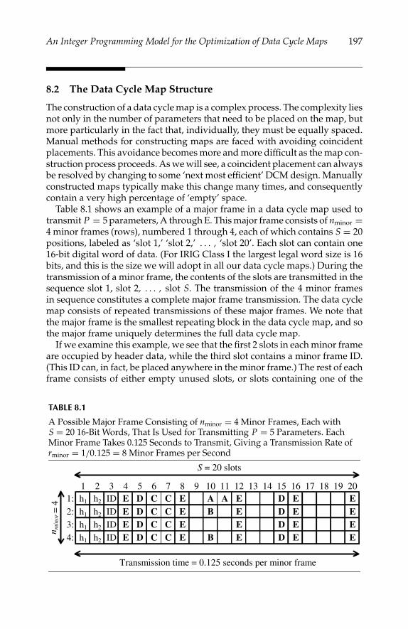
P1: shibu/Vijay

August 8, 2005 15:8 1914 1914˙C008

An Integer Programming Model for the Optimization of Data Cycle Maps 197

8.2 The Data Cycle Map Structure

The construction of a data cycle map is a complex process. The complexity liesnot only in the number of parameters that need to be placed on the map, butmore particularly in the fact that, individually, they must be equally spaced.Manual methods for constructing maps are faced with avoiding coincidentplacements. This avoidance becomes more and more difficult as the map con-struction process proceeds. As we will see, a coincident placement can alwaysbe resolved by changing to some ‘next most efficient’ DCM design. Manuallyconstructed maps typically make this change many times, and consequentlycontain a very high percentage of ‘empty’ space.

Table 8.1 shows an example of a major frame in a data cycle map used totransmit P = 5 parameters, A through E. This major frame consists of nminor =4 minor frames (rows), numbered 1 through 4, each of which contains S = 20positions, labeled as ‘slot 1,’ ‘slot 2,’ . . . , ‘slot 20’. Each slot can contain one16-bit digital word of data. (For IRIG Class I the largest legal word size is 16bits, and this is the size we will adopt in all our data cycle maps.) During thetransmission of a minor frame, the contents of the slots are transmitted in thesequence slot 1, slot 2, . . . , slot S. The transmission of the 4 minor framesin sequence constitutes a complete major frame transmission. The data cyclemap consists of repeated transmissions of these major frames. We note thatthe major frame is the smallest repeating block in the data cycle map, and sothe major frame uniquely determines the full data cycle map.

If we examine this example, we see that the first 2 slots in each minor frameare occupied by header data, while the third slot contains a minor frame ID.(This ID can, in fact, be placed anywhere in the minor frame.) The rest of eachframe consists of either empty unused slots, or slots containing one of the

TABLE 8.1

A Possible Major Frame Consisting of nminor = 4 Minor Frames, Each withS = 20 16-Bit Words, That Is Used for Transmitting P = 5 Parameters. EachMinor Frame Takes 0.125 Seconds to Transmit, Giving a Transmission Rate ofrminor = 1/0.125 = 8 Minor Frames per Second

1 2 3 4 5 6 7 8 9 10 11 12 13 14 15 16 17 18 19 201: h1 h2 ID E D C C E A A E D E E2: h1 h2 ID E D C C E B E D E E3: h1 h2 ID E D C C E E D E E4: h1 h2 ID E D C C E B E D E E

Transmission time = 0.125 seconds per minor frame

n min

or =

4

S = 20 slots

P1: shibu/Vijay

August 8, 2005 15:8 1914 1914˙C008


TABLE 8.2

Summary Statistics for Each Parameter in the Data Cycle MapDefined by Table 8.1 Assuming a Transmission Rate of rminor = 8Minor Frames per SecondParameter A B C D E

Period (slots) 80 40 20 10 4Occurrences per minor frame 0.25 0.5 1 2 5Occurrences per major frame 1 2 4 8 20Resultant sampling rate (samples/second) 2 4 8 16 40

5 parameters being transmitted. We note that each sampling of parametersB, D, and E generates data that occupies just a single slot; we say their wordrequirement is 1 slot. In this example, however, parameters A and C have aword requirement of 2 slots, and so we see that each occurrence of theseparameters occupies 2 adjacent slots in the map. Perhaps the most importantobservation is that each parameter appears with a regular period within themajor frame. For example, parameter D appears in every 10th slot in themajor frame, while parameter A appears just once in the major frame, and soappears in the data cycle map with a period of 80 slots.

Let us assume that for this example, we have a transmission rate of rminor =1/0.125 = 8 minor frames per second, and so 2 complete major frames aretransmitted every second. By counting the occurrences of each parameterin the major frame, we can compute the resultant sampling rates for eachparameter; this data is given in Table 8.2. In practice, the desired samplingrates will be given as part of the input data, and we then have to design adata cycle map that efficiently realizes (or exceeds) these desired rates for eachparameter.

We note that parameters A and B do not appear on every minor frame.Parameters such as these are said to be sub-commutated. On the other hand,parameters C, D, and E, which occur at least once on each minor frame, aresaid to be super-commutated. The use of these terms relates to the fact that theoriginal flight test instruments were electro-mechanical devices which usedcommutators to log the data.

In considering the application of optimization methods to data cycle mapconstruction we need to take into account our ability to manage the task interms of memory and computational requirements. For example, the construc-tion of an entire major frame, with its many repetitions of minor frames, willalmost certainly require a model which is too unwieldy and unmanageable.For this reason it will be necessary to decompose the problem into smallertasks whose solutions can be used as building blocks for solving the largerproblem. Our approach therefore will be to construct minor frames whosereplication can be used to define the entire major frame. In doing this it willbe essential that parameter sample rates are preserved and that parameterperiodicity is also achieved, along with other IRIG standards to be discussednext.

P1: shibu/Vijay

August 8, 2005 15:8 1914 1914˙C008


8.3 Designing a Minor Frame

The design of a suitable minor frame is dependent on several factors. Apartfrom periodicity and minimum required sample rates, IRIG Class I conditionsalso require that transmission bit rates fall within a minimum and maximumlevel, each minor frame has two header synchronization words and a minorframe ID word, there is a common word length for each parameter, minorframes contain no more than 512 16-bit words, and that there are no morethan 256 minor frames in a major frame. Although we will not be concernedwith many of these operational issues it is important that they are taken intoaccount when designing a suitable minor frame. We will assume that the twoheader words are placed at the beginning of each minor frame, but the frameID may be placed anywhere in the frame. Within these constraints the taskis to place the measured parameters onto a frame according to their requiredsample rates and periodicity. As we will see the periodicity will depend onthe size of the frame. There are normally several options available on the sizeof the frame, however it is our task to select the most efficient frame size.The efficiency E of a major frame is the ideal number of parameter words(excluding header words) transmitted per second divided by the actual totaltransmission rate:

E = ideal parameter words transmitted per secondtotal words transmitted per second

.

For any data cycle map, the number of words (including unused words cor-responding to empty slots) that are transmitted per second is given by theproduct of the minor frame length S and the minor frame rate rminor. Thenumber of words that actually need to be transmitted per second for someparameter p is given by rp × wp, where rp is the required sample rate (sam-ples/second) for parameter p, and wp is the word requirement (number ofwords that need to be transmitted per sample) for parameter p. Thus, theefficiency E of a solution with minor frame length S and minor frame raterminor can be written

E(S, rminor) =∑P

p=1 (rp × wp)

S × rminor, (8.1)

where P is the number of parameters. We note that the required number ofwords (in the numerator) does not include the header or frame ID words, eventhough these are needed in the data cycle map, and so, under this definition,100% efficiency can never be achieved. Alternative definitions are possible,but they do not significantly change the nature of the optimization problem.

For any given set of parameters, the efficiency E depends on the minorframe length S and the minor frame transmission rate rminor. Thus we cansplit our problem into a sequence of steps, being (1) to find a range of valuesfor S and rminor that define a number of candidate solutions, (2) choosing the

P1: shibu/Vijay

August 8, 2005 15:8 1914 1914˙C008


most efficient solution from among these candidates, and (3) then attempt-ing to find a placement of data parameters within the slots that satisfies theperiodicity requirements. Step (2) and Step (3) of this process may need to berepeated if a proposed best candidate is shown to be infeasible. Note that tokeep the solution times manageable, we will restrict ourselves to candidatesolutions that possess a specific intuitive structure. Although we believe thisstructure is likely to be possessed by an optimal solution, we cannot guaranteethat this is so, and so we cannot offer any formal guarantee of optimality.

We will show that once we have determined the minor frame rate rminor,it is reasonably straightforward to calculate a set of values for the minorframe length S that give rise to a family of candidate solutions. These candi-date solutions can be ordered from most efficient (but least likely to give afeasible placement) to least efficient (but guaranteed to be feasible). We alsoshow how to calculate the number of minor frames nminor required per majorframe for these solutions.

To illustrate our process, we will demonstrate the construction of a datacycle map for the following example.

Example 8.1Consider P = 5 parameters with sample rates rp and word requirements wp

as shown in Table 8.3.Our focus is on building minor frames, and hence we require that successive

minor frames be essentially the same in content. To achieve this, the trans-mission rate of each parameter needs to be an integer multiple (or fraction) ofthe minor frame transmission rate. This suggests that the minor frame trans-mission rate should be some integer multiple of at least one of the requiredparameter transmission rates. Transmitting a minor frame incurs the overheadof transmitting header and ID words, and so lower minor rates are likely to bebetter. Therefore, we choose to explore a set of candidate solutions in whichthe minor frame transmission rate matches the transmission rate of at leastone of the parameters.

In the process we will describe, we assume that the rp values are in increas-ing order, as is the case in Table 8.3. We now choose the minor frame rate rminorto be equal to the transmission rate rq of some parameter q , 1 ≤ q ≤ P , givingrminor = rq . (For ease of notation, we assume that parameter q is the first suchparameter with sampling rate rq , i.e., we break ties in transmission rates bychoosing the smallest q .) Note that some choices of q will be infeasible if they

TABLE 8.3

A 5-Parameter Data Set for Example 8.1Parameter A B C D E

Required sample rate (samples/second) rp 2 5 12 25 33Number of words required per sample wp 1 1 1 1 2

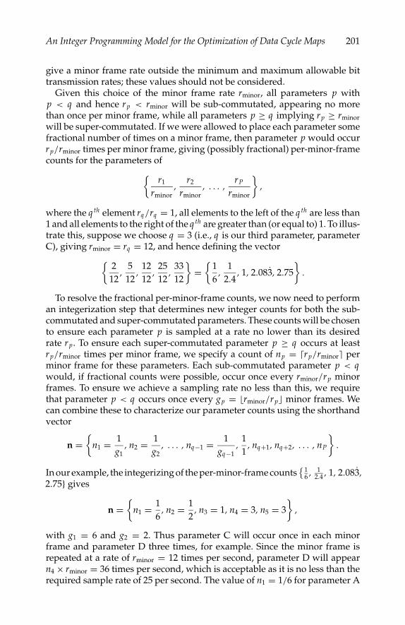
P1: shibu/Vijay

August 8, 2005 15:8 1914 1914˙C008


give a minor frame rate outside the minimum and maximum allowable bittransmission rates; these values should not be considered.

Given this choice of the minor frame rate rminor, all parameters p withp < q and hence rp < rminor will be sub-commutated, appearing no morethan once per minor frame, while all parameters p ≥ q implying rp ≥ rminorwill be super-commutated. If we were allowed to place each parameter somefractional number of times on a minor frame, then parameter p would occurrp/rminor times per minor frame, giving (possibly fractional) per-minor-framecounts for the parameters of

r1

rminor,

r2

rminor, . . . ,

rP

rminor

,

where the q th element rq /rq = 1, all elements to the left of the q th are less than1 and all elements to the right of the q th are greater than (or equal to) 1. To illus-trate this, suppose we choose q = 3 (i.e., q is our third parameter, parameterC), giving rminor = rq = 12, and hence defining the vector

2

12,

512

,1212

,2512

,3312

=

16

,1

2.4, 1, 2.083, 2.75

.

To resolve the fractional per-minor-frame counts, we now need to performan integerization step that determines new integer counts for both the sub-commutated and super-commutated parameters. These counts will be chosento ensure each parameter p is sampled at a rate no lower than its desiredrate rp. To ensure each super-commutated parameter p ≥ q occurs at leastrp/rminor times per minor frame, we specify a count of np = rp/rminor perminor frame for these parameters. Each sub-commutated parameter p < qwould, if fractional counts were possible, occur once every rminor/rp minorframes. To ensure we achieve a sampling rate no less than this, we requirethat parameter p < q occurs once every gp = rminor/rp minor frames. Wecan combine these to characterize our parameter counts using the shorthandvector

n =

n1 = 1g1

, n2 = 1g2

, . . . , nq−1 = 1gq−1

,11

, nq+1, nq+2, . . . , nP

.

In our example, the integerizing of the per-minor-frame counts1

6 , 12.4 , 1, 2.083,

2.75 gives

n =

n1 = 16

, n2 = 12

, n3 = 1, n4 = 3, n5 = 3

,

with g1 = 6 and g2 = 2. Thus parameter C will occur once in each minorframe and parameter D three times, for example. Since the minor frame isrepeated at a rate of rminor = 12 times per second, parameter D will appearn4 × rminor = 36 times per second, which is acceptable as it is no less than therequired sample rate of 25 per second. The value of n1 = 1/6 for parameter A

P1: shibu/Vijay

August 8, 2005 15:8 1914 1914˙C008


means that this parameter will occur only once in every g1 = 6 minor frames,giving a realized sampling rate of n1 × rminor = 2 samples per second, exactlymatching the required rate.

The next step is to calculate the number of minor frames nminor that will de-fine a complete major frame. Recall that nminor is simply the number of minorframes we have to observe before we see a repetition in the data being sent.If sub-commutated parameter p, p < q occurs once every gp minor frames,then the number of minor frames required is in general given by

nminor = LCM(g1, g2, . . . , gq ),

where the LCM() function computes the least common multiple of its argu-ments. This value will guarantee that the sub-commutated parameters can beperiodically placed on the minor frames. In our example g1 = 6, g2 = 2, andhence nminor = LCM(6, 2) = 6. Thus, parameter A must be placed in any oneof the 6 duplications of the minor frame which will make up the major frame.Parameter B must be placed in the same slot in every second minor frame,and so will appear 3 times in the major frame.

We next need to calculate the number of slots S required in the minor frameto ensure we can feasibly place all the parameters onto the data cycle map.We said earlier that there is a family of possible values of S, where smallervalues of S from this family are more efficient (i.e., more of the minor framecontains parameter data), but are less likely to permit a feasible parameterplacement (i.e., fewer slots are available to avoid coincident placements be-tween parameters). Our approach is to initially try a small value for S, andthen, if this does not allow a feasible parameter placement, keep increasingS until feasibility is achieved. This process will terminate by either finding aminor frame length that is feasible, or by generating a bit transmission ratethat exceeds the IRIG standards.

In our search for the best S, we need some sensible lower bound fromwhich we can start. A simple lower bound on S can be calculated by ignoringthe periodicity requirements, and simply counting up the number of datawords that need to be transmitted per minor frame. Each super-commutatedparameter p ≥ q has to occur np times per minor frame, thereby occupyinga total of npwp slots. Thus, the space required in each minor frame by thesuper-commutated data is given by

Ssuper =P∑

p=q

npwp.

For our example, we have Ssuper = (1 × 1)+ (3 × 1)+ (3 × 2) = 10. In additionto this, we need to reserve space for the sub-commutated parameters to ensurethere are no clashes between them and the other parameters. We note thatdifferent sub-commutated parameters can share the same slot position in theminor frames as long as we never need to transmit both parameters in thesame minor frame. Thus, in general, we need to solve some form of set packingproblem to determine how best to allocate the sub-commutated parameters to

P1: shibu/Vijay

August 8, 2005 15:8 1914 1914˙C008


slots and minor frames. However, a simple lower bound based on slot usageused can be easily calculated as

Ssub1 =

q−1∑p=1

npwp

.

Summing these values, and adding another 3 words for the header and IDwords, gives a lower bound on the minor frame length S:

S1 = Ssub1 + 3 + Ssuper.

For our example (Table 8.3), we have Ssub1 = 1

6 × 1 + 12 × 1 = 1, Ssuper = 10,

and so S1 = 10 + 3 + 1 = 14.We can strengthen this bound by considering the periodicity requirements.

Each super-commutated parameter p ≥ q must appear periodically in thedata cycle map, and so the minor frame length must be some multiple of eachsuper-commutated parameter’s per-minor-frame count np. Thus, we have

S = kLCM(np, p = q , q + 1, . . . , P), (8.2)

for some positive integer k. Thus, the lower bound S1 can be improved byincreasing it until it is a multiple of LCM(np, p = q , q + 1, . . . , P), giving anew bound of

S2 = k 2LCM(np, p = q , q + 1, . . . , P),

i.e., we have put k = k 2 in (8.2), where k 2 is the smallest integer value givingS2 ≥ S1. For our example, LCM(n3, n4, n5) = LCM(1, 3, 3) = 3, and so we in-crease our bound from S1 = 14 to S2 = 15. We note, as an aside, that increasingnp for some parameter p ≥ q could actually allow us to decrease the minorframe length S if it decreased this LCM value. This is not something we haveconsidered, but is left as a subject for future research.

We start our search by putting k = k 2, S = S2, and then try to place all theparameters into a major frame consisting of nminor minor frames of length S.We use integer programming to solve this problem; further details are pro-vided in the next section. If the integer program determines that no feasiblesolution exists, then we increase k by 1 in Equation (8.2), thereby increasingthe minor frame length S to the next multiple of the LCM. This process isrepeated until a feasible solution is obtained.

In Table 8.4 we show that it is possible to place all five parameters intoan (S × nminor) = (15 × 6) major frame constructed from minor frames de-fined by Table 8.5, and thus we have a feasible solution to our problem. Thekey parameter statistics for this solution, including the parameter periodsmp = S/np, are shown in Table 8.6. To summarize, we have 6 minor frames,each containing 15 words. Each word contains 16 bits. Parameter A will beplaced in only one of these minor frames (any one will do), parameter B willbe placed three times, once in every second minor frame, while parameters

P1: shibu/Vijay

August 8, 2005 15:8 1914 1914˙C008


TABLE 8.4

The Full Major Frame for the Example 1 Problem Defined in Table 8.3.In this Data Cycle Map, We Have nminor = 6 Minor Frames per Major Frame,a Transmission Rate of rminor = 12 Minor Frames per Second, and S = 15Slots per Minor Frame

1 2 3 4 5 6 7 8 9 10 11 12 13 14 15

1: h1 h2 D E E ID C D E E B D E E2: h1 h2 D E E ID C D E E A D E E3: h1 h2 D E E ID C D E E B D E E4: h1 h2 D E E ID C D E E D E E5: h1 h2 D E E ID C D E E B D E E6: h1 h2 D E E ID C D E E D E E

C, D, and E will be placed 1, 3, and 3 times respectively in each minor frame atappropriate positions that ensure periodicity. In this solution, minor framesare transmitted at the rate of rminor = 12 times per second. Using Equation(8.1), the efficiency E(S, rminor) of this solution is given by E(15, 12) = 110/

180 = 61.1%.The above process assumed we started by calculating a lower bound of

S1 = Ssub1 + 3 + Ssuper. In practice, we do not attempt to optimally allocate the

sub-commutated parameters, and so we do not use Ssub1 . Instead, we replace

the lower bound Ssub1 by the number of slots that must be reserved in each

minor frame for a heuristically generated parameter placement, which weconstruct as follows. Let Dsub be the number of distinct sub-commutated pa-rameters, where we say two such parameters are distinct if they have differentgp or wp values. Let (g′

d , w′d), d = 1, 2, . . . , Dsub be the set of distinct (gp,wp)

pairs found in the sub-commutated parameters, and let n′d , d = 1, 2, . . . , Dsub

be the number of sub-commutated parameters having (gp, wp) = (g′d , w′

d).A feasible allocation of the sub-commutated parameters is to pack the distinctparameters into their own slots within the minor frame. Therefore, the num-ber of minor-frame slots that we reserve for sub-commutated parameters isgiven by

Dsub∑d=1

⌈n′

d

g′d

⌉w′

d .

In practice, we replace Ssub1 by this value.

TABLE 8.5

One Possible Minor Frame Configuration for the Example 8.1 ProblemDefined in Table 8.3. Note That Slot 11 Is Reserved for Sub-CommutatedParameters A and B Who Share this Slot Position in the Major Frame1 2 3 4 5 6 7 8 9 10 11 12 13 14 15h1 h2 D E E ID C D E E AB D E E

P1: shibu/Vijay

August 8, 2005 15:8 1914 1914˙C008


TABLE 8.6

Sampling Rates for Each Parameter in The Data Cycle Map Definedby Table 8.5 Assuming a Transmission Rate of rminor = 12 MinorFrames Per SecondParameter A B C D E

Period mp 90 30 15 5 5Desired sampling rate rp 2 5 12 25 33Occurrences per minor frame np 1/6 1/2 1 3 3Resultant sampling rate nprminor 2 6 12 36 36

The process described above for Example 8.1 can be carried out for all pos-sible values of rq and an efficiency value E calculated for each. A number offactors may influence the value of E . These include the degree of roundingup required to determine the np values leading to over-sampling, the gap be-tween the minimal slot usage requirement S1, and the minor frame length S2required to satisfy periodicity, and any increases in k in Equation (8.2) requiredto permit a feasible parameter placement.

For very large data sets all or many of the values for S may violate themaximum minor frame length of 8192 bits. In this situation a simple de-vice for restoring legality is to introduce header splits into the minor frame.In this situation the header can be thought of as another parameter with asample rate determined by the required number of splits. For example, sup-pose that the most efficient frame design gives a frame length of 842 16-bitwords, including the original header of two words and a frame ID of oneword. We introduce another two word header and treat it as a parameterwith a sample rate of 2. The additional 2 words can be added to the origi-nal nominal minor frame length which will in most cases still give a framelength less than or equal to 842. If necessary the revised minor frame lengthS may need to be adjusted up by adding another LCM factor of the super-commutated parameters. When the new S value is computed (assume forthe sake of this argument this is still 842), our original minor frame of length842 can now be replaced by two minor frames each of length 421. Periodicplacement of the header will guarantee that it is placed at the start of each ofthese two new frames. The header splitting strategy will work as long as thetotal number of minor frames does not exceed the limit of 256. If this limitis exceeded, the data set is too large to conform to IRIG class I conditions forthis rminor.

Preprocessing of the data will examine all options for rminor and their rela-tive efficiencies. Under normal circumstances the option which has the high-est efficiency will be chosen, and we will then be able to create a feasibleminor frame for this configuration using the integer programming modeldiscussed next. Sometimes, however, the integer program will fail for the de-sired option, and so k in (8.2) will need to be increased by 1, changing thatoption to its next most efficient configuration. The new most efficient option

P1: shibu/Vijay

August 8, 2005 15:8 1914 1914˙C008


TABLE 8.7

A Data Set for Example 8.2 with 4 ParametersParameter A B C D

Required sample rate ri 1 3 3 5Number of words per sample wp 1 1 1 1

will then be solved using integer programming, with this process being re-peated until a feasible solution is found. Example 8.2 shows the results of thisprocess.

Example 8.2Consider the data given in Table 8.7.

Table 8.8 shows all possible rates, minor frame lengths, and efficiencies.Of the three possible frame rates the most efficient is a single frame withefficiency 80%.

The natural choice in this case is a frame rate of 1 with no sub-commutation.The periods mp = S/np for each parameter p are given by 15, 5, 5, 3 with aspace of 2 words reserved at the beginning for the header and an additionalspace for the frame ID. It is easy to show by construction that placement ofthe parameters on this frame is impossible without avoiding coincidence.In this case we are forced to try a less efficient frame construction withS = 2×LCM(1, 3, 3, 5) = 30. This S = 15 example fails because of the relativeprime relationship between the periods for parameters B and D (i.e., becausethese periods have no factors in common other than 1). In fact it can be shown[2] that a sufficient condition for the coincidence of parameters i and j inthe frame is that periods mi and m j are relatively prime. Panton et al. [2]explore the fact that other more complex relationships between the peri-ods also lead to coincidence. An interesting parallel with juggling is alsodiscussed.

In the discussion of the optimization models used to generate feasible place-ments which follows, we will assume that k in equation (8.2) has been in-creased to give an S for which no pair of parameters have periods that arerelatively prime.

TABLE 8.8

Alternative Frame Rates and Efficienciesfor Data from Table 8.7Option q rminor S E

1: 1 1 15 80%2: 2 3 8 50%3: 4 5 7 34%

P1: shibu/Vijay

August 8, 2005 15:8 1914 1914˙C008


8.4 Optimization Models

We now turn to the problem of finding a feasible placement of the parame-ters within a minor frame of length S with desired parameter periods mp. Weassume that the data set has been modified by removing all sub-commutatedparameters, and inserting in their place a set of new ‘aggregated’ parame-ters, each with per-minor-frame count np = 1, that represent the packed sub-commutated parameter solution generated by our heuristic.

Three models were considered for the generation of feasible placements.The first considered was an Integer Programming formulation in which pa-rameters were directly assigned to a minor frame with all desired properties.In this model we let xps be a binary decision variable whose value is 1 if param-eter p starts at position s on the minor frame and is 0 otherwise. This methodproved to be too slow to be operationally useful. It is well known [4], thatalthough this modeling approach is economic in terms of its proliferation ofvariables, the structure of the polytope is not conducive to finding solutionsefficiently. The second approach considered to generate feasible parameterplacements involved the use of Genetic Algorithms. A complete descriptionof this model can be found in [3].

8.4.1 Generalized Set Packing Model

The third approach was to employ a set packing model in which the columnsin the model represent all feasible placements for each individual parameter.Having determined the length of the minor frame S we can now enumerateall possible placements for a given parameter on this frame. Each placementpattern will be referred to as a tour. For example, consider the 4th parameter,parameter D in Table 8.6, which we require to appear n4 = 3 times in a minorframe of length S = 15 with a period of m4 = 5. This parameter will have thefollowing tours as shown in Table 8.9.

Our problem is to select one tour for each parameter so that each slot con-tains no more than one parameter. Generation of the parameter tours auto-matically ensures that they are periodic. Consider the following model.

Define the binary variable xp, j to be 1 if column j is selected for parameterp, and 0 otherwise. Our objective is then to:

[DCM] Maximize∑p, j

xp, j

subject to∑p, j

as,(p, j)xp, j ≤ 1 ∀ s,

∑j

xp, j = 1 ∀ p,

xp, j binary ∀ p, j.

P1: shibu/Vijay

August 8, 2005 15:8 1914 1914˙C008


TABLE 8.9

Enumeration of All Tours for a Parameterwith Period mp = 5 in a Frame of LengthS = 15

Tour

1 2 3 4 5

slot 1 1 . . . .slot 2 . 1 . . .slot 3 . . 1 . .slot 4 . . . 1 .slot 5 . . . . 1slot 6 1 . . . .slot 7 . 1 . . .slot 8 . . 1 . .slot 9 . . . 1 .slot 10 . . . . 1slot 11 1 . . . .slot 12 . 1 . . .slot 13 . . 1 . .slot 14 . . . 1 .slot 15 . . . . 1

where as,(p, j) = 1 if the j th column for parameter p covers slot s and 0 other-wise. Each row in the first block of constraints represents a slot in the minorframe. The second block of constraints ensure that only one column is selectedfrom each parameter set. This is a feasibility problem, and so the objectivefunction is essentially irrelevant.

Savings in the number of variables can be made by noting that in the genera-tion of the parameter tours there is considerable duplication since parameterswith the same minor frame sample rate and word requirements will have iden-tical tour sets. Parameters can be grouped into parameter classes and toursgenerated for each class. In this case the constraints which ensure that onlyone parameter is selected from each set are modified so that the appropri-ate number are selected from each class. Once the optimal solution is found,members of each class are assigned arbitrarily to each tour and the minorframe map reconstructed.

An interesting feature of this model is that we know a priori what theoptimal solution objective value is, since we know that all P parameters mustbe allocated. This enables us to set the tightest possible bound on the opti-mal solution, thereby greatly reducing the size of the branch and bound tree.Two other observations are important. First, when these models are solvedusing CPLEXTM 7.0, [5], we have the option of seeking feasible rather thanoptimal solutions since in this case any feasible solution is automatically op-timal. Second, Dual Simplex is used as the default linear program (LP) solver,however when the number of columns in the model becomes significantlygreater than the number of rows we switch to the Primal LP solver. Both ofthese strategies contribute significantly to reductions in execution times.

P1: shibu/Vijay

August 8, 2005 15:8 1914 1914˙C008


8.5 Strengthening the Set Packing Integer Programming Model

In addition to the issues discussed at the end of the last section, the nature ofthis problem lends itself to the addition of sets of clique inequalities whichwill considerably tighten the LP bounds and hence accelerate the solutionprocess. To summarize the requirements, we require that the pth parameter,p = 1, 2, . . . , P , be regularly spaced in the minor frame, and appear np times.We assume that np, p = 1, 2, . . . , P, are all positive integers, and the np val-ues are relatively prime, meaning that their greatest common divisor is 1.(This assumption is consistent with the np values defining relative, not abso-lute, transmission rates.) We note that to ensure periodicity, we have a minorframe length S = kLCM(np, p = 1, 2, . . . , P) where k ∈ 1, 2, 3, . . . . Thismeans that parameter p will occur every mp = S/np slots in the minor frame,where mp is the period of parameter p. We show in Appendix A , Theorem 8.1that

LCM(mp, p = 1, 2, . . . , P) = S.

The set packing integer programming model [DCM] for this problem hasS ‘slot’ constraints ensuring no more than 1 parameter occupies any slot, fol-lowed by P generalized upper bound (GUB) constraints that ensure that, foreach parameter, just one possible placement option from those that are legalis chosen. We will assume, until Section 8.5.2, that all wp = 1. Model [DCM]can be written in the form

[DCM] Maximize cT x

subject to Ax ≤ 1Gx = 1x ∈ 0, 1.

For ease of notation in this section, we number the slots, and the correspondingslot constraints, from 0, giving slot constraints 0, 1, 2, . . . , S−1. A parameterp with period mp has mp columns, and so we can consider the x vector to bepartitioned by parameters in the form x = (xp,0, xp,1, . . . , xp,mp−1), (p = 1,2, . . . , P). Variable xp, j = 1 if and only if parameter p occupies slots j, j +mp, j + 2mp, . . . , j + (np − 1)mp. In Ax ≤ 1, we have A = (as,(p, j)) withrows s = 0, 1, 2, . . . , S − 1 (one per slot) and columns indexed by (p, j),p = 1, 2, . . . , P, j = 0, 1, 2, . . . , mp − 1 where

as,(p, j) =

1 s ∈ j, j + mp, j + 2mp, . . . , j + (np − 1)mp0 otherwise.

That is, column (p, j) has 1’s in every mp’th row starting with row j , indicatingthat if column (p, j) is selected, parameter p will occupy every mp’th rowstarting with row j .

P1: shibu/Vijay

August 8, 2005 15:8 1914 1914˙C008


The slot constraints are of the form∑P

p=1∑mp−1

j=0 as,(p, j)xp, j ≤ 1, s = 0, 1,2, . . . , S − 1. From the definition of as,(p, j), we see that for any parame-ter p and any slot s, there is one and only one possible value of j whichresults in as,(p, j) = 1, i.e., in slot s containing parameter p. This occurs whens mod mp = j . Hence, we see that the slot constraints Ax ≤ 1 can be writtenin the form

P∑p=1

xp,s mod mp ≤ 1, s = 0, 1, . . . , S − 1. (8.3)

The GUB constraints Gx = 1 specify that exactly one placement is chosenfor each parameter, where gi,(p, j) = 1 for i = p, j = 1, 2, . . . , mp−1 andgi,(p, j) = 0 otherwise. The Gx = 1 constraints can also be expressed as

mp−1∑j=0

xp, j = 1, p = 1, . . . , P.

8.5.1 Pairwise Slot Constraints

In this section, we show how we can derive new pairwise slot constraintsfrom (8.3). These are examples of clique inequalities, and as such could bediscovered using normal conflict graphs, for example. However, we presentan explicit representation of the constraints, thereby allowing the discov-ery process to be bypassed. We also present a physical interpretation of theinequalities.

Let us consider two parameters, parameter p ∈ 1, 2, . . . , Pand parameterq ∈ 1, 2, . . . , P, p = q . Dropping the other parameters from (8.3) gives therelaxed constraint:

xp,s mod mp + xq,s mod mq ≤ 1, (8.4)

for any row s ∈ 0, 1, 2, . . . , S − 1.It is useful, at this stage, to define GCFpq = GCF(mp, mq ) to be the greatest

common factor (i.e., greatest integer divisor) for mp and mq . We can thendefine m′

p = mp/GCFpq and m′q = mq /GCFpq , and we note that m′

p and m′q are

relatively prime (i.e., their greatest common divisor is 1). The ratio m′p : m′

qdefines the interaction between parameters p and q in their slot usage. We alsonote that the least common multiple of mp and mq is given by LCM(mp, mq ) =GCFpq m′

pm′q .

Recall that S = LCM(m j , j = 1, 2, . . . , P) ≥ LCM(mp, mq ). For all valuesof s = 0, 1, . . . , S − 1 where s ≥ LCM(mp, mq ), we have both s mod mp = s ′

mod mp and s mod mq = s ′ mod mq where s ′ = s mod LCM(mp, mq ). There-fore, there are only LCM(mp, mq ) unique equations defined by (8.4), beingthose given by s = 0, 1, . . . , LCM(mp, mq ) − 1. Consider every mp’th ofthese constraints, starting with some constraint row (slot) r, 0 ≤ r < mp − 1.

P1: shibu/Vijay

August 8, 2005 15:8 1914 1914˙C008


There are LCM(mp, mq )/mp = (GCFpq m′pm′

q )/(m′pGCFpq ) = m′

q of these con-straints. We can sum these m′

q constraints to give:

r+(m′q −1)mp∑

s=r,r+mp,r+2mp, ...

(xp,s mod mp + xq,s mod mq ) ≤ m′q , r = 0, 1, . . . , mp − 1,

⇒r+(m′

q −1)mp∑s=r,r+mp,r+2mp, ...

(xp,r + xq,s mod mq ) ≤ m′q , r = 0, 1, . . . , mp − 1,

⇒ m′q xp,r +

r+(m′q −1)mp∑

s=r,r+mp,r+2mp, ...

xq,s mod mq ≤ m′q , r = 0, 1, . . . , mp − 1,

⇒ m′q xp,r +

m′q −1∑

j=0

xq,(r+ jmp) mod mq ≤ m′q , r = 0, 1, . . . , mp − 1,

⇒ m′q xp,r +

m′q −1∑

j=0

xq,r mod GCFpq + jGCFpq ≤ m′q , r = 0, 1, . . . , mp − 1.

(8.5)

where the last step follows from Theorem 8.3 in Appendix B.This equation has an intuitive physical interpretation that follows from

adopting parameter p’s view of the minor frame. This parameter’s slot usagerepeats every mp slots, and so from this parameter’s viewpoint there are onlymp different ‘positions of interest’. Each of these mp positions is realized asnp equally spaced slots in the minor frame. (Because of repetition, only m′

qof these have a unique interaction with parameter q . However, the equationis perhaps more intuitive if thought of as summing over repeated sets of m′

qslots, giving np slots in total.) By summing our equations, we are countinghow many of the slots used to realize this position are occupied by parametersp and q , for each of these mp positions of interest. The equation above specifiesthat the number of slots occupied in total by the parameters p and q cannotexceed the number of slots available.

Equation (8.5) can be strengthened by noting that if parameter q occupiesone of p’s positions of interest even just once in the minor frame, then pa-rameter p cannot occupy that position of interest without a clash occurringsomewhere in the minor frame. This motivates the following lifting of theabove equations.

Recalling that all the variables are binary, and only one xq, j variable for pa-rameter q can be at value 1, we see that the constraints in (8.5) can be strength-ened by increasing the coefficients on the xq,r mod GCFpq + jGCFpq variables from1 to m′

q , and then dividing through by m′q to give

xp,r +m′

q −1∑j=0

xq,r mod GCFpq + jGCFpq ≤ 1, r = 0, 1, . . . , mp − 1. (8.6)

P1: shibu/Vijay

August 8, 2005 15:8 1914 1914˙C008


This expression gives mp equations. We can form a set of new constraintsfrom (8.6) through appropriate summation of every GCFpq ’th of these equa-tions. For each value of e, e = 0, 1, . . . , GCFpq − 1, we can sum the equationsin (8.6) defined for r = e + jGCFpq , j = 0, 1, 2, . . . , m′

p − 1, where eachsummation includes mp/GCFpq = m′

p equations. This gives:

e+(m′p−1)GCFpq∑

r=e,e+GCFpq ,e+2GCFpq , ...

xp,r +

m′q −1∑

j=0

xq,r mod GCFpq + jGCFpq

≤ m′

p,

e = 0, 1, . . . , GCFpq − 1

⇒m′

p−1∑k=0

xp,e+kGCFpq +

m′q −1∑

j=0

xq,(e+kGCFpq ) mod GCFpq + jGCFpq

≤ m′

p,

e = 0, 1, . . . , GCFpq − 1

⇒m′

p−1∑k=0

xp,e+kGCFpq +

m′q −1∑

j=0

xq,e mod GCFpq + jGCFpq

≤ m′

p,

e = 0, 1, . . . , GCFpq − 1

⇒m′

p−1∑k=0

xp,e+kGCFpq + m′p

m′q −1∑

j=0

xq,e+ jGCFpq ≤ m′p,

e = 0, 1, . . . , GCFpq − 1.

As before, the GUB constraints allow us to lift these constraints by increasingthe coefficients on xp,e+kGCFpq from 1 to m′

p, and then dividing through by m′p

to give

m′p−1∑

j=0

xp,e+ jGCFpq +m′

q −1∑j=0

xq,e+ jGCFpq ≤ 1, e = 0, 1, . . . , GCFpq − 1,

⇒α∑

j=0

xp,e+ jGCF(mp,mq ) +β∑

j=0

xq,e+ jGCF(mp,mq ) ≤ 1,

e = 0, 1, . . . , GCF(mp, mq ) − 1. (8.7)

where α = mp/GCF(mp, mq )−1, and β = mq /GCF(mp, mq )−1. Equation (8.7)gives a set of valid inequalities for each pair of parameters. These can be usedto strengthen the relaxed linear programming form of [DCM], thus makingit easier to solve to integrality.

8.5.2 Multi-Word Parameters

We now consider a model where the number of bits required to transmit aparameter exceeds those of a slot, and so the parameter occupies more thanone consecutive slot in the data cycle map.

P1: shibu/Vijay

August 8, 2005 15:8 1914 1914˙C008


Let us assume that parameter p requires wp consecutive slots (words)each time it is transmitted. Clearly, we require the number of words to beless than the parameter’s period mp, i.e., wp < mp. The j th column xp, j , j = 0,1, . . . , mp − 1, for parameter p now defines the case where parameter p oc-cupies slots h, h + 1, . . . , h + wp − 1 for all h = j, j + mp, j + 2mp, . . . , j +(np − 1)mp.

To keep the model form consistent with the wp = 1 case, we include columnsin the model in which a parameter occupies ‘consecutive’ slots that wraparound from the end of the frame back to the beginning. For example, someparameter p with wp = 3 might occupy the slots S− 1, 0, and 1. Any solutionlike this can be interpreted as a valid solution by renumbering the slots sothat slot 0 occurs at the start, not the middle, of the parameter’s slot usage.Alternatively, if reducing symmetry in the formulation is important, thenvariables such as these can be forced to zero using additional constraints thatleave the underlying model form intact.

In the wp = 1 model, slot s was used by parameter p if parameter p wasplaced in position j = s mod mp, i.e., if slot j was the first slot occupied byparameter p. In the new model, the same slot s will be used if parameter pis placed in position j , or any of the wp − 1 preceding positions. Thus, theconstraint for slot s, Equation (8.3), now becomes

P∑p=1

wp−1∑h=0

xp,(s mod mp)−h ≤ 1, s = 0, 1, . . . , S − 1,

where we assume modulo mp wrap around for xp, j in the sense that xp,−1 =xp,mp−1, xp,−2 = xp,mp−2, etc.

Proceeding as before, we relax this constraint to consider only the twoparameters p and q , giving

wp−1∑h=0

xp,(s mod mp)−h +wq −1∑h=0

xq,(s mod mq )−h ≤ 1, s = 0, 1, . . . , S − 1.

We can then add the equations as before, noting that each occurrence ofxp, j mod mp is replaced by

wp−1h=0 xp,( jmod mp)−h, and similarly for xq, j mod mq . This

gives the following general form of Equation (8.5):

wp−1∑h=0

m′q xp,r−h +

m′q −1∑

j=0

wq −1∑h=0

xq,(r mod GCFpq + jGCFpq )−h ≤ m′q , r = 0, 1, . . . , mp − 1.

(8.8)

Before we lift this equation, we note that if wq < GCFpq , then each xq,k variablethat appears in the summation appears exactly once. If wq = GCFpq , then,by considering the r = 0 case, we see that the second summation includesvariables xq,k for all k ∈ jGCFpq − h : j = 0, 1, . . . , m′

q − 1; h = 0, 1, . . . ,GCFpq − 1. Given m′

q GCFpq = mq , we see that this includes all of the mq

possible variables defined for parameter q . In this case, the GUB constraint

P1: shibu/Vijay

August 8, 2005 15:8 1914 1914˙C008


on the xq,k variables implies m′

q −1j=0

wq −1h=0 xq,(r mod GCFpq + jGCFpq )−h = 1 for all r ,

and so xp,k = 0 ∀ k is the only solution to this equation. Thus, there is nofeasible solution to the problem if wq = GCFpq , or indeed if wq is larger thanthis, implying that physically parameter q requires more consecutive slots,and so the problem is more tightly constrained. The same argument applies,by symmetry, to wp, and so we see that a feasible solution can only exist ifwp < GCFpq and wq < GCFpq . From now on, we will restrict ourselves tothis case.

As before, we proceed to lift Equation (8.8), which gives:

wp−1∑h=0

xp,r−h+m′

q −1∑j=0

wq −1∑h=0

xq,r mod GCFpq + jGCFpq −h ≤ 1, r = 0, 1, . . . , mp−1. (8.9)

This expression gives mp equations. As before, we can form a set of newconstraints from (8.9) through appropriate summing of every GCFpq ’th ofthese equations. For each value of e, e = 0, 1, . . . , GCFpq − 1, we can sum theequations in (8.9) defined for r = e + jGCFpq , j = 0, 1, 2, . . . , m′

p − 1. Eachsummation includes mp/GCFpq = m′

p equations. This gives:

e+(m′p−1)GCFpq∑

r=e,e+GCFpq ,e+2GCFpq , ...

wp−1∑

h=0

xp,r−h +m′

q −1∑j=0

wq −1∑h=0

xq,(r mod GCFpq + jGCFpq )−h

≤ m′

p,

e = 0, 1, . . . , GCFpq − 1

⇒m′

p−1∑k=0

wp−1∑

h=0

xp,e+kGCFpq −h +m′

q −1∑j=0

wq −1∑h=0

xq,(e+kGCFpq ) mod GCFpq + jGCFpq −h

≤ m′

p,

e = 0, 1, . . . , GCFpq − 1

⇒m′

p−1∑k=0

wp−1∑

h=0


q −1∑j=0

wq −1∑h=0

xq,e mod GCFpq + jGCFpq −h

≤ m′

p,

e = 0, 1, . . . , GCFpq − 1

⇒m′

p−1∑k=0

wp−1∑h=0

xp,e+kGCFpq −h + m′p

m′q −1∑j=0

wq −1∑h=0

xq,e+ jGCFpq −h ≤ m′p,

e = 0, 1, . . . , GCFpq − 1.

Using the same arguments as before, we can lift the coefficients to give:

m′p−1∑

k=0

wp−1∑h=0


q −1∑j=0

wq −1∑h=0

xq,e+ jGCFpq −h ≤ 1, e = 0, 1, . . . , GCFpq −1.

Thus, if we have wp < GCFpq and wq < GCFpq then we can strengthen ourmodel using the above valid inequalities. If the restrictions on wp and wq arenot satisfied, then no feasible solution exists to the problem.

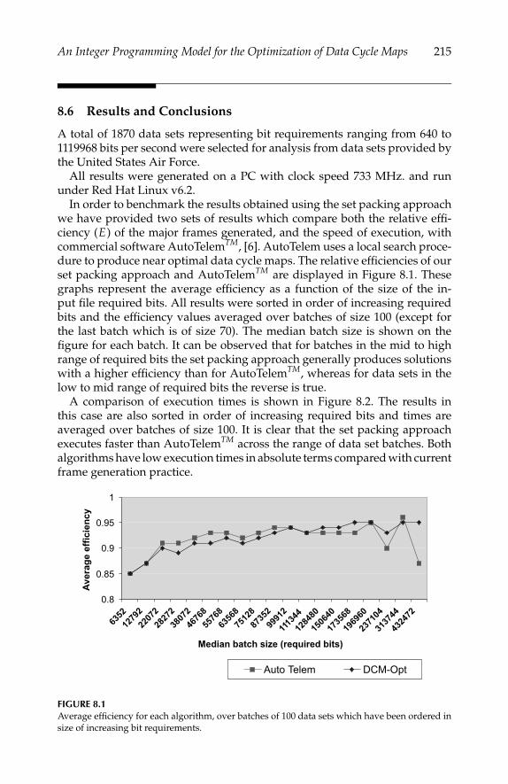
P1: shibu/Vijay

August 8, 2005 15:8 1914 1914˙C008


8.6 Results and Conclusions

A total of 1870 data sets representing bit requirements ranging from 640 to1119968 bits per second were selected for analysis from data sets provided bythe United States Air Force.

All results were generated on a PC with clock speed 733 MHz. and rununder Red Hat Linux v6.2.

In order to benchmark the results obtained using the set packing approachwe have provided two sets of results which compare both the relative effi-ciency (E) of the major frames generated, and the speed of execution, withcommercial software AutoTelemTM, [6]. AutoTelem uses a local search proce-dure to produce near optimal data cycle maps. The relative efficiencies of ourset packing approach and AutoTelemTM are displayed in Figure 8.1. Thesegraphs represent the average efficiency as a function of the size of the in-put file required bits. All results were sorted in order of increasing requiredbits and the efficiency values averaged over batches of size 100 (except forthe last batch which is of size 70). The median batch size is shown on thefigure for each batch. It can be observed that for batches in the mid to highrange of required bits the set packing approach generally produces solutionswith a higher efficiency than for AutoTelemTM, whereas for data sets in thelow to mid range of required bits the reverse is true.

A comparison of execution times is shown in Figure 8.2. The results inthis case are also sorted in order of increasing required bits and times areaveraged over batches of size 100. It is clear that the set packing approachexecutes faster than AutoTelemTM across the range of data set batches. Bothalgorithms have low execution times in absolute terms compared with currentframe generation practice.

0.8

0.85

0.9

0.95

1

6352

1279

2

2207

2

2827

2

3807

2

4676

8

5576

8

6356

8

7512

8

8735

2

9991

2

1113

44

1284

80

1506

40

1735

68

1969

60

2371

04

3137

44

4324

72

Median batch size (required bits)

Ave

rag

e ef

fici

ency

Auto Telem DCM-Opt

FIGURE 8.1Average efficiency for each algorithm, over batches of 100 data sets which have been ordered insize of increasing bit requirements.

P1: shibu/Vijay

August 8, 2005 15:8 1914 1914˙C008


0

10

20

30

40

6352

1279

2

2207

2

2827

2

3807

2

4676

8

5576

8

6356

8

7512

8

8735

2

9991

2

1113

44

1284

80

1506

40

1735

68

1969

60

2371

04

3137

44

4324

72

Median batch size (required bits)

Ave

rag

e ti

me

(sec

s)

AutoTelem DCM-Opt

FIGURE 8.2Average execution time in seconds for AutoTelemTM and the set packing approach, over batchesof 100 data sets which have been ordered in size of increasing bit requirements.

We have described a fast and flexible method for the generation of TelemetryFrames or Data Cycle maps which has provided high efficiencies for large op-erationally realistic data sets. The method is flexible in the sense that changesin frame construction rules can easily be implemented using this modelingapproach. Execution times are sufficiently small to suggest that even largerdata sets can be accommodated in the future, and are several orders of mag-nitude lower than times taken at present to create Telemetry Frames usingcomputer assisted methods. The set packing approach has also been shownto compare very favorably with the commercial software AutoTelemTM bothin terms of speed and efficiency.

Acknowledgments

This work was partly sponsored by an internal ITEE Divisional Grant from theUniversity of South Australia and also by United States Air Force Contractnumber F04700-00-P-1181. The authors wish to acknowledge the valuableimprovements made to this paper by the referees.

References

1. Telemetry Group, Range Commanders Council, IRIG Standard 106-96, Teleme-try Standards, Secretariate, Range Commanders Council, U.S. Army WhiteSands Missile Range, NM, May 1996.

2. Panton, D., John, M., Lucas, S., and Mason, A., Flight test data cycle map opti-misation, EJOR, 146, 486, 2003.

P1: shibu/Vijay

August 8, 2005 15:8 1914 1914˙C008


3. John, M., Optimisation models for the generation of data cycle maps and re-gional surveillance, Ph.D. thesis, University of South Australia, Mawson Lakes,Australia, 2003.

4. Johnson, E. L., Nemhauser, G. L., and Savelsbergh, M. W. P., Progress in lin-ear programming-based algorithms for integer programming: An exposition,INFORMS Journal on Computing, 12, 1, 2000.

5. ILOG CPLEX 7.0, ILOG INC., Mountain View CA.6. AutoTelem, QUEST Integrated Inc.

Appendix A: LCM Proof

In this appendix, we show that LCM(mp, p = 1, 2, . . . , P) = S where S = k LCM(np, p = 1, 2, . . . , P), k ∈ 1, 2, 3, . . . , and mp = S/np.

LEMMA 8.1Consider the calculation of LCM(np, p = 1, 2, . . . , P). Let np = z∈zr p

z ,p = 1, 2, . . . , P, where = 2, 3, 5, . . . is the set of prime numbers, and r p

z ∈1, 2, 3, . . . is the integer power associated with z ∈ in the prime factorization ofnp. (For example, if we have n1 = 60 = 223151, then r2

1 = 2, r31 = 1, r5

1 = 1, r71 =

0, . . . ) By definition, we have LCM(np, p = 1, 2, . . . , P) ≡ z∈zmaxp=1,2, ... , P r pz .

LEMMA 8.2LCM(k × np, p = 1, 2, . . . , P) = k × LCM(np, p = 1, 2, . . . , P) for k ∈ 1, 2,3, . . . .

PROOF This follows easily from Lemma 8.1 by considering the prime fac-torization of k and then rearranging.

THEOREM 8.1LCM(mp, p = 1, 2, . . . , P) = S.

PROOF From the definition mp = S/np, we need to show that LCM(S/np,p = 1, 2, . . . , P) = S, where S = k LCM(np, p = 1, 2, . . . , P) for anyk ∈ 1, 2, 3, 4, . . . . Firstly, we note that all S/np, p = 1, 2, . . . , P are strictlypositive integer values, and so the LCM is well defined. As in Lemma 8.1, weconstruct prime factorizations giving np = z∈zr p

z , p = 1, 2, . . . , P , where is the set of prime numbers, and r p

z ∈ 0, 1, 2, . . . is the power associ-ated with z ∈ in the factorization of np. Similarly, let S = z∈zrz , whererz = maxp=1,2, ... , P r p

z , z ∈ defines the prime factorization of S. We notethat because the np values, p = 1, 2, . . . , P are relatively prime (i.e., theironly common divisor is 1) we have the key observation that

minp∈1,2, ... , P

r pz = 0 ∀ z ∈ . (8.10)

P1: shibu/Vijay

August 8, 2005 15:8 1914 1914˙C008


Using Lemma 8.1, we have

LCM(

Snp

, p = 1, 2, . . . , P)

= LCM

( ∏z∈ zrz∏

z∈pzr p

z, p = 1, 2, . . . , P

),

= LCM

(∏z∈

zrz−r pz , p = 1, 2, . . . , P

),

=∏z∈

zmaxp=1,2, ... , P (rz−r pz ),

=∏z∈

zrz−minp=1,2, ... , P r pz ,

=∏z∈

zrz ,

where the last simplification follows from (8.10). As S = z∈zrz , the result isproven.

Appendix B: Equivalency Proofs

In this section, we prove several equivalencies between sets of values.

THEOREM 8.2The set ( jm′

p)modm′q , j = 0, 1, . . . , m′

q − 1 = 0, 1, 2, . . . , m′q − 1 when m′

pand m′

q are relatively prime.

PROOF We note that this set has m′q values, each between 0 and m′

q − 1inclusive. We will show, by contradiction, that these values are all unique,and hence the result will follow.

Assume that two of these values are equal, i.e., ( jm′p) mod m′

q = (( j +k)m′

p) mod m′q = ([( jm′

p) mod m′q ] + [(km′

p)mod m′q ]) mod m′

q , where inte-gers j and k satisfy 0 ≤ j < j + k < m′

q . For this to be true, we require(km′

p) mod m′q = 0, implying km′

p is an integer multiple of m′q , i.e., km′

p = k ′m′q

for some positive integer k ′. But, because m′p and m′

q are relatively prime, thesmallest value of k for which this is true is k = m′

q (from LCM(m′p,m′

q ) = m′pm′

qwhen m′

p and m′q are relatively prime). This value of k is outside the range per-

mitted, and thus we have a contradiction. Therefore, all the values, between0 and m′

q − 1 must be distinct, and so the result follows.

THEOREM 8.3The set of indices R = (r + jmp)mod mq , j = 0, 1, . . . , m′

q −1 = r1, r2, . . . , rm′q

with ri+1 = ri + GCFpq , and r1 = rmodGCFpq , where GCFpq = GCF(mp, mq ),the greatest integer divisor common to mp and mq , and we define m′

p = mp/GCFpq

and m′q = mq /GCFpq .

P1: shibu/Vijay

August 8, 2005 15:8 1914 1914˙C008


PROOF We observe that (r + jmp) mod mq = (r +[( jmp) mod mq ]) mod mq .We also note that ( jmp) mod mq = ( jGCFpq m′

p) mod (GCFpq m′q ) = GCFpq

[( jm′p) mod m′

q ]. This allows us to write

R = (r + GCFpq [( jm′p) mod m′

q ]) mod mq , j = 0, 1, . . . , m′q − 1.

Using Theorem 8.2, we can rewrite this as

R = (r + j ∗ GCFpq ) mod mq , j = 0, 1, . . . , m′q − 1. (8.11)

Noting that mq = GCFpq m′q , we see that jGCFpq < mq ∀ j = 0, 1, . . . , m′

q −1,and so the successive values in set R must differ by GCFpq , allowing usto write R = r1, r2, . . . , rm′

q where ri+1 = ri + GCFpq , 1 ≤ i < m′

q − 1. Wenote that the set ‘wraps’ in the sense that (rm′

q+ GCFpq ) mod mq = r1. We also

observe that r1 = r mod GCFpq . This r1 value follows from the observationthat the smallest value in R must lie between 0 and GCFpq − 1 inclusive.The wrap property of R means that we can remove the bounds on j in (8.11)without changing the contents of R. By putting j = −r/GCFpq we haver + jGCFpq = r −r/GCFpq GCFpq = r mod GCFpq , showing that r1 as definedabove is indeed a member of R. This completes the proof.

P1: shibu/Vijay

August 8, 2005 15:8 1914 1914˙C008

P1: shibu/Vijay

August 10, 2005 11:57 1914 1914˙C009

9Application of Column GenerationTechniques to Retail Assortment Planning

Govind P. Daruka and Udatta S. Palekar

CONTENTS

9.1 Introduction . . . . . . . . . . . . . . . . . . . . . . . . . . . . . . . 2219.2 Literature Review . . . . . . . . . . . . . . . . . . . . . . . . . . . . 2249.3 Problem Description . . . . . . . . . . . . . . . . . . . . . . . . . . 230

9.3.1 Expected Revenue/Profit Functions (ER/PF) . . . . . . . . 2309.3.2 Constraints on Assortment . . . . . . . . . . . . . . . . . . 231

9.4 Mathematical Model . . . . . . . . . . . . . . . . . . . . . . . . . . 2329.4.1 Problem Decomposition . . . . . . . . . . . . . . . . . . . . 2339.4.2 Mathematical Formulation of Buyer’s Problem . . . . . . . 2349.4.3 Mathematical Formulation of the Subproblems . . . . . . . 236

9.4.3.1 Carry/No Carry Rules . . . . . . . . . . . . . . . . 2379.4.4 Algorithmic Considerations . . . . . . . . . . . . . . . . . . 238

9.5 Computational Results . . . . . . . . . . . . . . . . . . . . . . . . . 2399.5.1 Algorithm Performance on Base Data . . . . . . . . . . . . 2399.5.2 Effect of Problem Parameters . . . . . . . . . . . . . . . . . 242

9.5.2.1 Effect of Package Quantity . . . . . . . . . . . . . 2439.5.2.2 Effect of Number of Replenishments . . . . . . . 2449.5.2.3 Effect of Inventory Holding Cost . . . . . . . . . . 2459.5.2.4 Effect of Number of Assortments . . . . . . . . . . 2469.5.2.5 Effect of Profit Margin . . . . . . . . . . . . . . . . 247

9.6 Conclusions . . . . . . . . . . . . . . . . . . . . . . . . . . . . . . . 248References . . . . . . . . . . . . . . . . . . . . . . . . . . . . . . . . . . . 248

9.1 Introduction

The retail industry is one of the largest sectors of commerce worldwide andis the second largest in the U.S. both in the number of establishments and thenumber of employees. In the U.S. the retail trade presently generates about

221

P1: shibu/Vijay

August 10, 2005 11:57 1914 1914˙C009


3.8 trillion dollars in retail sales annually and accounts for about 12.9% of allbusiness establishments (U.S. Census [42]).

Retailers must estimate the likelihood of sales for each item and also eval-uate the trade-off between different items due to limited availability of retailspace in the store and other constraints. This task is very complex due tothe almost infinite product variety, inherent variability in product demand,and significant errors in forecasting demand. Since space constraints do notallow all products to be carried, the retailer must select a limited number ofproducts. The set of products carried in a store is termed as the assortment ofproducts. The products in a store typically form a hierarchy. A line of productcan have multiple items in it and each item can have multiple stock keepingunits (SKUs). SKUs are at the lowest level of the product hierarchy. For exam-ple, if shoes of a particular pattern are an item then the different shoe sizesform the SKUs for the item.

The product assortment decision is one of the key issues faced by retailers.Retailers need to decide the number of different merchandizing categoriesthey would like to keep within a store or department, referred to as productvariety or the breadth of the assortment, as well as the number of (SKUs) theyshould carry within a category, referred to as the depth of the assortment orinventory depth. Retailers also need to decide the brands they would carry forthe chosen categories namely store brands, local brands, and national brands,which affects the pricing across categories.

Retailers are driven by consumers who have high expectations for ser-vice and product excellence and yet demand lower prices. Intense com-petition and rapidly changing consumer tastes have resulted in increasedturnover rate in most product categories (Chong et al. [9]). In response, re-tailers are addressing these new demands in different ways. Some retailersare focusing on aggregating their overall needs from a supplier or groupof suppliers to establish greater buying leverage but the process, time, andtechnology constraints introduce significant difficulty in accomplishing andsustaining this task. Some retailers change their assortment frequentlyaccording to perceived changes in demographic, economic, or seasonal de-mand patterns, but the consequent investment in retail space and inventorycan be prohibitively expensive. Some retailers carry larger inventories witha higher risk of these inventories becoming obsolete and simultaneouslyincur higher inventory costs. Meeting marketing and financial planning obli-gations, forces most retailers to take the easy approach to merchandizingrepeating the assortment breadth and depth from previous seasons, creatingstore assortments based on store volume and ranking items by sales volumealone. This leads to the creation of a few standard product assortments typ-ically based on store size, which are then deployed throughout the chain ofstores. However, mismatches of chain wide strategies and local consumerneeds can lead to significant lost sales due to out-of-stock conditions or dis-tress sales due to overstock conditions. Pashigan [31] shows that the costs

P1: shibu/Vijay

August 10, 2005 11:57 1914 1914˙C009

Application of Column Generation Techniques to Retail Assortment Planning 223

incurred by retailers due to markdowns have been increasing in the U.S. ap-parel industry.

Retailers must address the customer’s needs by aligning the merchandiz-ing processes such as strategic and financial planning, assortment and spaceplanning, inventory deployment, and in-season management. The merchan-dizing process is a systems approach, aimed at maximizing return on invest-ment, through planning sales and inventory in order to increase profitability,by maximizing sales potential and minimizing losses from markdowns andstock-outs. A comprehensive approach would be to balance the demands ofconsumers and the constraints of operating a retail business profitably bytransforming the merchandizing process by having an intelligent assortmentand category-planning process that accommodates the entire merchandizingprocesses.

Assortment planning involves asking questions such as: Which product?How much of it? What colors? What sizes? Where to place it? Who is the tar-get customer? and so on. Assortment planning is the decision making processthat a retailer undertakes to determine the correct mix of items to be carried byeach store so as to maximize the opportunity for sale. Decisions are made re-garding what to keep (assortment width) and how much to keep (assortmentdepth) in a store. Assortment planning directly affects the product selection,pricing, timing, and micro-merchandizing. By employing a proper assortmentplanning solution the retailer can gain immensely since the product assort-ment matched with market potential and inventory aligned with sales lead toincreased sales, fewer markdowns, and improved margins. This detailed planof action also helps in improving employee morale and the overall efficiency.Thus the retailer can provide better service to customers and simultaneouslyavoid carrying large inventory and the consequent higher inventory costs,and reduce the risk of inventory obsolescence.

In the previous decade, large retailers have invested heavily in informationtechnology. Point-of-sale scanners coupled with massive databases allowretailers to gather information in real time. However, there are very fewtools that make effective use of this data for the purpose of planning assort-ments to maximize sales. Most commercial software facilitate the assortmentplanning process by providing database connectivity and user-friendly in-terfaces. However, very little optimization and decision making capability isprovided.

In this paper we present a mathematical model of assortment planningwhich provides a decision support system that addresses the problem ofassortment width as well as the assortment depth. We address the problem ofa single period assortment planning problem with stochastic demand undershelf space, inventory turns, and various returns-on constraints. We formulatethe problem as a Linear Integer Programming problem and use a columngeneration technique to solve the model. The model was implemented by alarge chain of department stores for assortment planning.

P1: shibu/Vijay

August 10, 2005 11:57 1914 1914˙C009


9.2 Literature Review

Research on issues related to assortment planning dates back to the earlyyears of Operations Research. Whitin [43] noted that for the retail stores, theinventory control problem for style goods is further complicated by the factthat inventory and sales are not independent of one another. An increase ininventories may bring about increased sales of some items but a decrease insales of other items. Cairns [7] proposes that the business of a retailer can beregarded as selling the retail space at their disposal to their suppliers. Theretail space should, therefore, be allocated to those products that give themaximum profit.

A significant amount of research has been done since then on the impor-tance of inventory and shelf space in assortment decisions. Fox [14] describesthe importance of assortment planning process in retail industry. Cox [11]measured the relationship between sales of an individual product brand andits shelf space. The model was tested in six supermarkets where the shelfspace inventory of the two test products — powdered coffee cream and salt —over two leading brands in each category were varied each day, while keep-ing the total shelf space for these two categories constant. Shelf space wasshown to affect sales volume while location on shelves was not significant.Frank and Massy [15] take sixty three weeks of store audit data and use mul-tiple regression analysis to estimate the parameters of their two basic models.They conclude that by varying the number of facings of a brand in a shelfdisplay increases sales for high but not low volume SKU’s. They also con-clude that there is minimal or no effect of the shelf level or height and thereis absolutely no effect whether the product is kept at floor or any other shelfrow. Curhan [12] proposes a model to explain the space elasticity as a func-tion of several product-specific variables and tests this model under actualoperating conditions for nearly five hundred grocery products over five totwelve weeks before and after changing the space allocation. He finds thereis a positive relationship between shelf space and unit sales. Similar resultswere obtained by Wolfe [45] who concludes based on his empirical experi-ment that the sales of style merchandize, such as women’s dresses or sportsclothes, are proportional to the amount of inventory displayed. Other stud-ies by Levin et al. [26], Schary and Becker [33], Silver and Peterson [36],Larson and DeMarais [24] show that the retail display inventory has an stim-ulating effect on the customers which can lead to increased sales. Urban [41]presents a generalization of the inventory-level-dependent demand inventorymodels that explicitly models the demand rate as a function of the displayedinventory level and makes an explicit distinction between the back room anddisplayed inventories. The special case of full-shelf merchandizing, in whichthe product is replenished as soon as the back room inventory is depleted, isalso presented. Then they consider the product assortment and shelf-space

P1: shibu/Vijay

August 10, 2005 11:57 1914 1914˙C009


allocation problems by extending this model into a multi-item, constrainedenvironment.

Marketing models treat a product as a vector of attributes with customers’utility function defined over those attributes. Lancaster [23] provides a sum-mary of this research. These models focus on choosing a product line to max-imize the expected utility of the customer by either designing products withdesirable attributes or choosing preexisting products which possess suchattributes (Green and Krieger [16], Urban [40], Shocker and Srinivasan [35]).Urban [39] develops a mathematical model for product line decisions to iden-tify which products should be included in a firm’s product line. Product linedecisions are difficult to make because the products in the line are not usu-ally independent. Interdependency is the key consideration in such decisionmaking. A comprehensive discussion of marketing models for product lineselection can be found in Lilien et al. [27].

A large body of literature addresses the issue of assortment selection andallocation of limited retail shelf space for established commodity productstypically sold in a supermarket. Anderson and Amato [1] formulate a modelto determine the most profitable, short run brand mix concomitant with adetermination of the optimum allocation of a fixed product display areaamong available brands. This model when solved gives the compositionof the specific brands that should be displayed, and the amount of dis-play area that should be assigned to these brands, in order to maximizeprofit. Bultez and Naert [6] consider this problem by using marginal analysisof the profit function. They assume individual product demand is knownand develop a generalized framework to allocate shelf space for an assort-ment with interacting demand. Based on this framework, they develop apractical allocation rule called Shelf Allocation for Retailers’ Profit(SHARP). They discuss the special conditions under which SHARP reducesto the various rules of thumb commonly employed by retailers. However,in this framework, they do not explicitly consider which products to in-clude in their assortment and assume that substitution between products issymmetric.

Borin et al. [3] consider the joint assortment selection and space allocationproblem. It is assumed that demand is generated from the inherent charac-teristics of a product, the allocated shelf space, the selection of the assort-ment, and the stock levels of other products. The estimates of the parameterscapturing these effects were estimated using regression analysis. Demand isassumed to be known and deterministic through functions involving theseparameters. The objective was to maximize return on inventory subject tospace constraints. The model was solved based on a heuristic using thesimulated annealing technique, to select an assortment of ketchup in thesupermarket.

Mahajan and Ryzin [29] developed a theoretical model to determine thenumber and type of colors for seasonal and replenishable products. They

P1: shibu/Vijay

August 10, 2005 11:57 1914 1914˙C009


suggest that with each additional item, the total demand for the product lineincreases, but demand uncertainty across each item also increases, thus in-creasing overstocking and understocking costs. To determine the numberand type of items before this increase in revenue is offset by such costs, themodel considers groups of items corresponding to a product defined as acategory and assumes that the demand across these items is generated bycombining a multinomial logit choice process with a Poisson arrival pro-cess for the customer. The resulting Poisson distribution of demand wasapproximated to a normal distribution and was linked to the retailers’ in-ventory costs by a newsboy model. Based on the assumptions of the demandprocess, structural results were developed to answer the question regardinghow these items should be included in the assortment corresponding to thisproduct. Kahn and Lehmann [20] found preference for an assortment to bepositively related to individual item preference, an additional item’s unique-ness relative to the existing assortment, and the total number of items in theassortment.

For fashion products, assortment planning issues were addressed moredirectly by Smith and Agrawal [38] who considered the joint problem of as-sortment selection and optimal stocking for a group of products at a givenlevel. Demand was modelled as negative binomial random variable. The non-linear model developed has as its objective function, the cost function of thenewsboy problem which represents the total inventory costs of overstockingand understocking products. The model is solved using numerical meth-ods. Mahajan and Ryzin [30] analyze a single-period, stochastic inventorymodel (newsboy-like model) in which a sequence of heterogeneous customersdynamically substitute among product variants within a retail assortmentwhen inventory is depleted. The customer choice decisions are based on autility maximization criterion. The retailer must choose initial inventorylevels for the assortment to maximize expected profits. The authors proposeand analyze a stochastic gradient algorithm for the problem, and prove that itconverges to a stationary point of the expected profit function under mild con-ditions. The authors give numerical examples to show that the substitutioneffects can have a significant impact on an assortment’s profits.

There are several assortment models dealing with issues similar to theone presented in this chapter. Rajaram [32] models the problem of fashion re-tail assortment planning as a nonlinear integer programming problem withassumption that the retailer places a single order for all the products. Thedemand is modelled as a random variable and the constraint set includes abudget constraint which is later expanded to include shelf space constraint.To solve the model an upper bound for the problem is developed by relax-ing the budget constraint. The solution obtained corresponding to the upperbound may not be feasible due to violation of budgetary constraint and soto achieve feasibility they develop a Lagrangian heuristic and a two-phaseheuristic as an alternative approach. Corstjens and Doyle [10] developed a

P1: shibu/Vijay

August 10, 2005 11:57 1914 1914˙C009


shelf-space allocation model in which they considered the demand rate as afunction of shelf space allocated to the product and also applying a polyno-mial functional form of demand with main- and cross-elasticities of shelfspace, they utilized signomial geometric programming to solve the model.Zufryden [48] suggested the use of dynamic programming to solve theshelf-space allocation problem, as it will allow general objective-functionspecifications and will provide integer solutions.

In the above two articles an assumption is made that all of the inventoryis on display which is generally not appropriate for retail stores such as gro-cery stores. Also these models do not account for the location factors. In viewof these limitations Yang and Chen [47] proposed a simplified integer pro-gramming model based on the model developed by Corstjens and Doyle [10].The objective function is linearized by assuming that the profit of any prod-uct is linear with respect to a range of facings for which it is displayed bycontrolling the lower and upper bounds for that product. They also do notconsider the product availability constraint assuming that the product avail-ability is no longer an issue in the present market scenario. The model thenresembles a multi-knapsack problem which is solved in multiple stages. Yang[46] presents a heuristic algorithm that extends the greedy algorithm used forknapsack problems to solve the above model. The profit of each item perdisplay length on a particular shelf is treated as a weight, and the rankingorder of weight is used as a priority index in the process of space allocation.The heuristic procedure can allocate a product with lower profit to a shelfin order to satisfy the lower bounds for the product. To improve the heuris-tic procedure solution, an adjustment phase consisting of three adjustmentmethods is proposed. These adjustment methods improve the heuristic so-lution but are not useful if there is variation in the length of facings of theproducts. To overcome this shortcoming, Lim et al. [28] propose new neigh-borhood moves namely multi-shift, multi-exchange, and multi-add-exchangeand solve the Yang and Chen [47] model employing a strategy of combininga strong local search with metaheuristics. They also develop a network flowsolution approach to solve the model as a minimum cost maximum flowproblem. They further incorporate the cross product affinity effect amongproducts such that there will be additional profit by having two particularproducts on the same shelf and considering a nonlinear base profit function.They obtained near-optimal solutions for small number product-shelf rangesand consistently good results for all other ranges tested.

Hoch et al. [18] present a general mathematical model of variety based onthe complete information structure of an assortment, defined by the multi-attribute structure of the objects and their spatial locations. The model isused to develop assortments that vary widely in terms of their informationstructure. The influence of variety perception and organization on statedsatisfaction and store choice was investigated. Information structure has abig impact on variety perceptions, though diminishing returns accompany

P1: shibu/Vijay

August 10, 2005 11:57 1914 1914˙C009


increases in the number of attributes on which object pairs differ. Customersare more influenced by local information structure (adjacent objects) thannonlocal information structure and the organization of the display can eitherincrease or decrease variety perceptions. Jayaraman et al. [19] address theproblem of jointly determining the product variety decision with the order-ing decision for the variations of a brand of a certain product that comprisea particular product line by modelling it as a nonlinear optimization model.Assumptions are made that the consumer preferences for products are knownand are ordinally scaled for the subset of products in the product line and canbe added or deleted according to profitability criterion.

The impact of product assortment on an individual’s decisions is examinedby Chernev [8] by conducting four experiments using fifty to one hundredundergraduates from Northwestern University as respondents for differentexperiments. They conclude that the impact of assortment on individual de-cision processes and choice is moderated by the degree to which individ-uals have articulated attribute preferences. Individuals with an articulatedideal point are more likely to prefer larger assortments than individualswithout articulated preferences. Shelby and Miller [34] consider the shop-per’s joint decision of item selection and pricing to determine the best as-sortment to carry in terms of profit maximization. They specifically consideritem complementarity and substitution with respect to profit implications forthe retailer. Koelemeijer and Oppewal [22] tackle the question of what is theoptimal assortment in a very different purchasing situation — those involvedwith a frequently purchased category like cut flowers. They choose this cate-gory because there is no branding, no stockpiling, and no packaging. In thistype of category, variety seeking and bundling issues become relevant. Theirmodel provides a tool to allow for optimization of retail assortments by con-sidering substitution, complementarity, and asymmetric dominance effects.Simonson [37] reviews and synthesizes recent empirical evidence indicatingthat product assortments can play a key role, not only in satisfying customers’wants, but also in influencing what they want. He shows that retailers canuse the considered assortment to change the likelihood that a consumer willmake a purchase, and to affect the probability that a specific option will bechosen.

Stassen et al. [25] consider assortment decisions across multiple stores.When consumers are shopping among several stores, a retailer needs toconsider whether his or her assortment should compete with the compe-tition (thinking of the stores as substitutes) or complement the competition(thinking of stores as complements). In this sense, the assortment de-cision can be thought of as an element of the marketing mix in attractingconsumers into the store. Their empirical results based on market datafor a specific market show that the assortment decision reflects a compet-itive relationship rather than a complementary one. Furthermore, the as-sortment decision was shown to be as important, if not more important, asthe price.

P1: shibu/Vijay

August 10, 2005 11:57 1914 1914˙C009


Evaluation of competing assortments has also received attention in litera-ture. Chong et al. [9] present an empirically based modelling frameworkfor managers to assess the revenue and lost sales implication of alterna-tive category assortments. The framework consists of a category-purchase-incidence model and an extended version of the classical brand-share modelof Guadagni and Little [17]. The brand-share model predicts which brandthe customer chooses if a purchase incidence occurs in the category. Dhruvet al. [13] use Data Envelopment Analysis to account for sales differencesin stores for a multi-chain retailer given differences in category assortmentsand regional preferences. Because regional preferences vary and the assort-ments carried by each store are different it is not appropriate to comparethem directly to assess performance. This method establishes a best prac-tice benchmark so stores within the chain can be fairly evaluated. A numberof studies have shown that brands and brand sizes can be reduced withoutaffecting sales or consumers’ perceptions of variety (Williard Ltd. and Inc.[44], Broniarcyzk et al. [5]). What constitutes efficient assortments is likely tovary in different categories and in different shopping environments (Kahnand McAlister [21]). Brijs et al. [4] tackle the problem of product assortmentanalysis by introducing a concrete microeconomic integer programmingmodel for product selection (PROFSET) based on the use of frequent itemsets. They demonstrate its effectiveness on real-world sales transaction dataobtained from a fully-automated convenience store.

From marketing literature it is known that the optimal product assortmentshould meet two important criteria. First, the assortment should be qualita-tively consistent with the store’s image. The retailer’s background knowledgewith regard to basic products should be easily incorporated in the model bymeans of additional constraints. A store’s image distinguishes the retailerfrom its competition and is projected through its design, layout, services, andof course its products. Second, because retailing organizations are profitseeking companies, the product assortment should be quantitatively appeal-ing in terms of the profitability it generates for the retailer. Most of the modelsthat address the problem of assortment planning are mathematical modelsthat are either nonlinear or involve integrality constraints which makes thesemodels computationally hard to solve. Accordingly, most of them use heuris-tics or relaxations of the problem to reach a solution. Most of the models do notconsider the inter-dependence between decisions for two or more items exceptfor satisfying them on a more or less ad-hoc basis during postprocessing ofsolution. Finally, the problem is solved for one store at a time. This leads to in-dividually customized assortments. This proliferation of assortments makesit difficult for chain stores to devise a consistent presentation across all stores.Most of the models also do not adequately treat the availability of back-roomspace or the retailers desire to maintain high inventory turnover rates. Finally,many of the models are unwieldy in terms of the number of parameters thatmust be estimated making it difficult to scale up to large practical problemsolving.

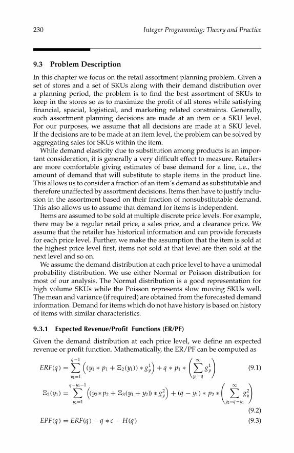
P1: shibu/Vijay

August 10, 2005 11:57 1914 1914˙C009


9.3 Problem Description

In this chapter we focus on the retail assortment planning problem. Given aset of stores and a set of SKUs along with their demand distribution overa planning period, the problem is to find the best assortment of SKUs tokeep in the stores so as to maximize the profit of all stores while satisfyingfinancial, spacial, logistical, and marketing related constraints. Generally,such assortment planning decisions are made at an item or a SKU level.For our purposes, we assume that all decisions are made at a SKU level.If the decisions are to be made at an item level, the problem can be solved byaggregating sales for SKUs within the item.

While demand elasticity due to substitution among products is an impor-tant consideration, it is generally a very difficult effect to measure. Retailersare more comfortable giving estimates of base demand for a line, i.e., theamount of demand that will substitute to staple items in the product line.This allows us to consider a fraction of an item’s demand as substitutable andtherefore unaffected by assortment decisions. Items then have to justify inclu-sion in the assortment based on their fraction of nonsubstitutable demand.This also allows us to assume that demand for items is independent.

Items are assumed to be sold at multiple discrete price levels. For example,there may be a regular retail price, a sales price, and a clearance price. Weassume that the retailer has historical information and can provide forecastsfor each price level. Further, we make the assumption that the item is sold atthe highest price level first, items not sold at that level are then sold at thenext level and so on.

We assume the demand distribution at each price level to have a unimodalprobability distribution. We use either Normal or Poisson distribution formost of our analysis. The Normal distribution is a good representation forhigh volume SKUs while the Poisson represents slow moving SKUs well.The mean and variance (if required) are obtained from the forecasted demandinformation. Demand for items which do not have history is based on historyof items with similar characteristics.

9.3.1 Expected Revenue/Profit Functions (ER/PF)

Given the demand distribution at each price level, we define an expectedrevenue or profit function. Mathematically, the ER/PF can be computed as

ERF(q ) =q−1∑y1=1

((y1 ∗ p1 + 2(y1)) ∗ g1

y

)+ q ∗ p1 ∗

( ∞∑y1=q

g1y

)(9.1)

2(y1) =q−y1−1∑

y2=1

((y2∗ p2 + 3(y1 + y2)) ∗ g2

y

)+ (q − y1) ∗ p2 ∗

( ∞∑y2=q−y1

g2y

)

(9.2)EPF(q ) = ERF(q ) − q ∗ c − H(q ) (9.3)

P1: shibu/Vijay

August 10, 2005 11:57 1914 1914˙C009


where q is the quantity kept in the store and q/ρ ∈ Z+, ρ is the packagequantity of the SKU, g j

y is the probability of selling yj units at level j , p j isthe selling price at level j , and c is the purchase price. The g j

y’s are computedfrom the demand distribution that is used. j (.) are calculated recursively byvarying the parameters in each recursion. The depth of recursion is equal tothe price levels in the problem.

In the equation for EPF(q ), H(q ) is the cost of holding a quantity q over thespecified period of time. It is calculated as

H(q ) = q2n

∗ h (9.4)

where h is the holding cost and n is the number of replenishments. The hold-ing cost for q units as calculated above is an approximation to the expectedholding cost since it assumes uniform demand over the planning horizon.

Given the demand distribution, these functions estimate the variation ofrevenue and profit with increasing SKU quantity in the store. EPF is the singleperiod news-vendor objective function which has been modified to accommo-date demand at different price levels. It is assumed that any residual inventoryis discarded at the end of the period, incurring a loss equal to the cost of theSKU. ER/PF functions are nonlinear and therefore difficult to use. However,we simplify the problem by using a piecewise linear approximation. For lowvolume SKUs we linearize the problem by considering break points at eachdiscrete value. For a high volume SKU we divide the ER/PF function curveinto several discrete segments on both sides of the maximum point and con-sider break points at those segments. The accuracy of this method dependson the number of segments used to approximate the EPF.

The revenue function ERF(q ) is a nondecreasing function that asymptot-ically approaches the value ERF(∞) whereas profit function EPF(q ) is uni-modal. This implies that as the quantity of a particular SKU increases in astore, the profit initially increases but after reaching a maximum, starts tofall. This is because beyond the point of maximum profit, the probability ofselling an extra unit of the SKU is sufficiently small so that the expected re-alized profit becomes smaller than the expected loss due to not selling thatadditional unit. This results in an overall decline in the Profit function.

We denote the point of maximum profit on the profit function by EPF(q ∗)and the corresponding point on the revenue function by ERF(q ∗). The averagesale price of a SKU is then obtained by calculating ERF(q ∗)/q ∗.

9.3.2 Constraints on Assortment

Since it is important to ensure that stores present a consistent appearanceto customers to create brand recognition, it is important that the number ofdifferent assortments that are created is limited. Accordingly, a retailer maylimit the number of different assortments that can be used. Such a restrictionwill obviously reduce the expected profit but it also reduces the cost asso-ciated with maintaining a large number of assortments. It is also easier to

P1: shibu/Vijay

August 10, 2005 11:57 1914 1914˙C009


create a store image that is consistent. One way to permit more customiza-tion for stores is to use a modular planogram. In such a planogram, oneconstructs smaller sub-assortments and the store then selects from the sub-assortments to create its planogram. Since several sub-assortments may carrythe same item, it is important that an item is in only one of the sub-assortmentsselected.

The choice of assortment can also be restricted based on financial criteria.There may be a limit on the total dollar value of inventory that a store can carry.This may limit the use of certain planograms which have multiple facings ofthe same item and therefore require a larger amount of inventory to appearfilled. Inventory may also be constrained in the form of constraints on thenumber of inventory turns that the store must provide. Thus an assortmentmust be picked such that the ratio of the sales to the average inventory is abovea given threshold. Thus a planogram with multiple facings may require alarge amount of inventory and not perform as well as one with fewer facings.An overall budget constraint may be used across the entire line of itemsand across the entire chain of stores. Such constraints can be used to modelwhat retailers call “open to buy”. The budget is the maximum dollar valuethat the chain will invest in system-wide inventory for a specific productline.

Space considerations limit the number of planograms or sub-assortmentsthat can be stored in a store. Space can either be a display space or back roomspace. Backroom or storage space is used when the amount of display spaceis inadequate to accommodate the inventory amount that must be stored inthe store. Depending on the maximum number of replenishments that arepermissible for a store and the package quantities for the item, the displayspace may not be adequate to hold the peak amount of inventory. In suchcases, it is important to ensure that sufficient back room space is provided.Clearly, back room space is to be used only if the item is part of the assortmentand therefore assumed to be on display.

9.4 Mathematical Model

Given a set of SKUs and stores, there are an exponential number of ways togenerate strategies which makes it impossible to generate all possible strate-gies and pick the best among them. Therefore, we formulate the assortmentplanning problem as a Mixed Integer Programming problem and decomposeit into two parts, the master problem and the subproblem, which can be solvedusing a Column Generation technique (Bazaraa et al. [2]). The subproblemreturns improved strategies based on the set of space related dual variablespassed to it by the master problem. The method is discussed in greater detailin subsequent sections.

The assortment for a store is constrained by several different requirements.These constraints result from the availability of display and storage space,

P1: shibu/Vijay

August 10, 2005 11:57 1914 1914˙C009


from advertising related legal requirements, and from performance require-ments. There are also further restrictions caused by the presentation of itemsin the store. This last aspect of the problem is called planogramming. Aplanogram is a preset collection of related items that are arranged on displayfixtures to gain maximum visibility and impact. While commercial softwareto draw the planograms exists, such software does not take a global view ofthe problem in terms of system performance. The assortment planning modelmust therefore also consider the problem of generating planograms.

Our model uses a two-level approach. This allows us to divide the probleminto what we call the Buyer’s problem (technically, the master problem) andthe Plannogrammer’s problem (technically, the pricing sub-problem). Thelower level Planogrammer’s problem generates planogram proposals or sub-assortments based on information supplied with placing items in a store. TheBuyer’s problem then evaluates the sub-assortments so generated and assignsthem to appropriate stores such that all restrictions are met and the objectivefunction is maximized. This is an iterative process in which the two problemsare alternately solved until the optimal solution is obtained.

The objective of the model is to select an assignment of sub-assortmentsto stores so as to maximize the expected profit while ensuring that the as-signment uses only a prespecified number of assortments, satisfies spaceavailability at the store, and achieves on the aggregate level a prespecifiednumber of inventory turns.

Details of the mathematical model and explanation of the various con-straints in the two problems are given below.

9.4.1 Problem Decomposition

The Buyer’s Problem is to assign existing sub-assortments to stores so asto maximize the overall revenue or profit of the system. Any assignmentcan use at most a prespecified number of sub-assortments. The assignmentof sub-assortments to stores must meet various restrictions including thoseon inventory values and turns and various space constraints. These variousrestrictions and constraints in the model are discussed in the following sub-section.

The Planogrammer’s Problem (PP) is to use the solution of the Buyer’sProblem and generate a suitable new sub-assortment or plan which will in-crease the revenue/profit in the Buyer’s Problem.

When the model for the Buyer’s Problem is solved, along with the assign-ment of sub-assortments to store, we obtain information that can be used tofind the value of having a new sub-assortment for each store. The Planogram-mer’s Problem is to come-up with a new sub-assortment that fits in the displayspace available for the store and has the maximum possible value. Solvingthis model yields a new sub-assortment which can be added to the Buyer’sProblem. This process can be repeated until it is not possible to find a new sub-assortment for any store. At this point, the final assignment of sub-problemto stores can be made.

P1: shibu/Vijay

August 10, 2005 11:57 1914 1914˙C009


We use the following notation in the mathematical description of the model.

Parameters:I : number of SKUs.J : number of stores.K : number of planograms.T : number of linear segments used to approximate the EPF.i : index of SKUs.j : index of stores.k : index of planograms.t : index of linear segments.s : system or retailer wide stock to sales ratio.S : maximum system stock in dollars.M : maximum number of planograms allowed.Z : A large integer value.pi : average sale price of SKU i .li : length of SKU i .Ki : set of planograms containing SKU i .s j : stock to sales ratio for the store j .b j : back-room linear space in store j .l f

j : fixture length in store j .I j : maximum inventory in dollars of aggregate of SKUs in store j .di j : maximum depth of SKU i allowed in store j .ni j : maximum number of replenishments for SKU i in store j per year.l pk : length of planogram k.

Wi jt : piecewise linear approximation of qi j .ri jt : profit (revenue) for Wi jt amount in store.

Decision variables:Xi j : amount of SKU i in back-room in store j .qi j : total quantity of SKU i in store j .Yi j : number of facings of SKU i in store j .aik : number of facings of SKU i in planogram k.

Zk =

1 : if planogram k is selected by some store0 : otherwise

Zkj =

1 : if store j selects planogram k0 : otherwise

9.4.2 Mathematical Formulation of Buyer’s Problem

max∑

t

∑j

∑i

rijtWijt

∑t

∑j

∑i

Wijt − qij = 0 ∀ i, j (9.5)

qij − dijYij − Xij ≤ 0 ∀ i, j (9.6)

Xij + Yij − qij ≤ 0 ∀ i, j (9.7)

P1: shibu/Vijay

August 10, 2005 11:57 1914 1914˙C009


∑i

pi qij ≤ I j ∀ j (9.8)

∑i

pi (0.5 − s j nij)qij ≤ 0 ∀ j (9.9)

∑j

∑i

pi qij ≤ S (9.10)

∑j

∑i

pi (0.5 − snij)qij ≤ 0 (9.11)

∑i

li Xij ≤ b j ∀ j (9.12)

Xij − ZYij ≤ 0 ∀ i, j (9.13)

Yij −∑kεKi

aik Zkj = 0 ∀ i, j (9.14)

∑k

l pk Zkj ≤ l f

j ∀ j (9.15)

∑kεKi

Zkj ≤ 1 ∀ i, j (9.16)

∑k

Zk ≤ M (9.17)

Zkj − Zk ≤ 0 ∀ k, j (9.18)

In the above model, the objective function is to maximize the expectedrevenue or profit where we are using the piece-wise linear approximation ofthe ER/PF. Constraint (9.5) ensures that the linearization of ER/PF functionis consistent.

Constraint (9.6) to Constraint (9.9) are inventory related constraints. Con-straint (9.6) ensures that the total store inventory for an SKU cannot exceed theamount of space on display shelves plus the amount kept in the back-room.Thus, with Yij facings the maximum amount of SKU i on display shelves ofstore j can be at most dijYij and then the maximum amount of SKU i in thestore j becomes the sum of dijYij and the back-room quantity Xij. Constraint(9.7) ensures that the total quantity is at least equal to the back-room quantityand as many items as there are facings in the front room. Constraint (9.8) ismade active if the maximum inventory value for the store has been specified.The value of the inventory in the store is calculated as the sum of sellingprice of each SKU times the total quantity of the SKU in the store. The sellingprice of the SKU can vary from store to store. This constraint ensures that theaggregate dollar value of inventory of all the SKU’s in store j is less than themaximum dollar value of inventory specified for that store. Constraint (9.9)is store level stock-to-sales ratio constraint. This constraint ensures that theaverage inventory (half the total inventory) must be less than the stock-to-sales ratio specified times the total demand that can be satisfied. If the target

P1: shibu/Vijay

August 10, 2005 11:57 1914 1914˙C009


number of turns cannot be met then no item will be carried in the store. Notethat, there is an inherent assumption in this constraint that the average salesrate is constant over the period of interest. While this may not be entirelyaccurate, stock-to-sales ratio constraints are applied over the average inven-tory over longer intervals of times such as months or quarters and hence theconstant sales rate assumption is practically reasonable. Further note that theinventory is valued at selling price. It is relatively easy to convert inventoryvaluation to cost price.

Constraint (9.10) and Constraint (9.11) are budget related constraints.Constraint (9.10) is the retailer or system level investment constraint and itensures that the total investment by the retailer for all the SKUs in all the storesis less than the specified maximum retailer investment stock in dollar value.Constraint (9.11) is retailer or system level stock-to-sales ratio constraint.

Constraint (9.12) to Constraint (9.16) are space related constraints. Con-straint (9.12) is the back-room space constraint and it ensures that the amountof space used by inventory of all the SKUs in the store does not exceed theback-room space available for the store. Constraint (9.13) is the front-backspace constraint and it ensures that inventory of a SKU is kept in the back-room only if at least one facing of the SKU is displayed in the front-room or thedisplay space of the store. Constraint (9.14) is the facing space constraint and itcalculates the number of facings of each SKU based on the assignment of sub-assortments to the store and the facings in each sub-assortment. Notice, thateach planogram has a given number of facings, aik , for each SKU i . Thus the to-tal number of facings for an SKU i is given by kεKi aik Zkj . This number affectsthe total displayed inventory in Constraint (9.7). Since the planograms are de-signed by the subproblem, the number of facings in a planogram are designedto best utilize the available display space. Constraint (9.15) is the front-roomor display space constraint and it ensures that the total display space used bythe sub-assortments assigned to the store is no more than the space available.Constraint (9.16) is the only-one SKU constraint and it ensures that two sub-assortments assigned to a store cannot have a SKU in common. This restrictionhas been included from marketing point of view for aesthetic reasons and itavoids the problem of having the same SKU at two ends of the assortments.

Constraint (9.17) and Constraint (9.18) are planogram related constraints.Constraint (9.17) ensures that the total number of sub-assortments or plans se-lected for all the stores combined do not exceed the maximum number of plansallowed. Constraint (9.18) ensures that the total number of sub-assortmentsor plans selected for a store do not exceed the maximum number of plansallowed for a store.

9.4.3 Mathematical Formulation of the Subproblems

For subproblems, we use the following additional notations.

Parameters:s : index of shelf.Mis : maximum amount of SKU i on a shelf s.

P1: shibu/Vijay

August 10, 2005 11:57 1914 1914˙C009


L p : maximum length of planogram allowed for a store .Fij : dual variable for the Constraint (9.14).Dj : dual variable for the Constraint (9.15).Oij : dual variable for the Constraint (9.16).

Decision variables:xi : multiplicity of SKU i in a planogram.yis : multiplicity of SKU i on shelf s.

zi =

1 : if SKU i is in planogram0 : otherwise

The model is:

ν j = min −∑

i

Fijxi + Dj L p +∑

i

Oijzi (9.19)

∑i

li yis ≤ L p ∀ s (9.20)

∑s

yis = xi ∀ i (9.21)

yis ≤ Mis zi ∀ i, s (9.22)

Constraint (9.20) is planogram length constraint and it ensures that the cal-culated sum of length of each SKU times the number of SKUs on the shelfdoes not exceed the maximum allowable length of the planogram for all theshelves. Constraint (9.21) ensures that the aggregate number of SKU i on allshelves is equal to the total number of SKU i in the planogram. Constraint(9.22) ensures that the total number of SKUs i on shelf s does not exceed themaximum allowable amount of SKU i on shelf s.

The length L p depends on the physical shelves that are available in a store.If more than one type of shelving system is available, then the length L p canbe varied to create planograms of different lengths. This allows for creationof standardized modules that can be used across multiple stores. Thus, evenif a planogram module is created for a single store, it is possible to use itacross all stores. Alternatively, it is possible to restrict the stores in which aparticular planogram is used. This can be achieved by not creating columnscorresponding to the restricted stores in the master problem.

9.4.3.1 Carry/No Carry Rules

Carry/No Carry rules allow the user to force the decision for a specific SKU.The user may require that certain SKUs are carried in specific stores due tomarketing or advertising requirements. Alternatively, certain SKUs may notbe allowed in certain stores due to local restrictions. The sub-problem can bemodified in this case to set the specific zi to be either 1 or 0 depending onwhether the SKU must be carried or not. In the event that we set zi = 1 wealso require xi ≥ 1. Moreover, the resulting planogram is assigned to onlythose stores which match the carry/no carry rule.

P1: shibu/Vijay

August 10, 2005 11:57 1914 1914˙C009


9.4.4 Algorithmic Considerations

The column generation scheme outlined above would be adequate if the prob-lem was a linear programming problem. Unfortunately, the master problemhas integer variables and thus column generation is not guaranteed to give theoptimal solution and may not even give a feasible integer solution. Ideally onewould use a branch-and-price methodology, which uses a column generationat each node of the branch and bound tree. However, given the size of theproblem we are solving, it is unlikely to be computationally feasible to solvethe problem in a reasonable amount of time using branch-and-price. Our ex-perience thus far shows that solving an integer program using the columnsgenerated for the LP relaxation almost always gives a feasible solution andthe solution so obtained is generally quite good. However, even in this case,the column generation schema generates a large number of sub-assortmentswhich results in an enormous master problem. Accordingly, we have to re-strict the number of sub-assortments that are generated. Since the problemis solved across a large number of stores, it is possible that such a restrictionmay or may not be able to generate assortments that are suitable for everystore. To ensure that many stores are able to contribute to the sub-assortmentgeneration problem, we use one of several strategies:

• Restriction : Each store is allowed to generate no more than a fixednumber of sub-assortments. This allows more stores to generatesub-assortments. Moreover, stores with differing amounts of salescan be given priority in generating the sub-assortments to get widerrepresentation in the sub-assortments that are generated.

• Grouping by Sales : The stores can be grouped into a number ofgroups using the average demand vector for the different items.This will allow stores with similar sales patterns to cluster together.A composite store can be constructed using the average of demandsacross each store within a cluster and this composite store can beused to generate the sub-assortments.

• Grouping by Size : Stores can alternatively be grouped by the totalsales for the product line in the store. This usually works well ifthere are significant differences in available space at different stores.A composite store can again be created. Notice that this approachlooses most of the individual differences between stores of a similarsize.

• Grouping by Sales and Size : This approach combines both of theabove criteria for clustering stores. This is done by adding the totalsales as one more of the attributes of the store.

The use of the grouping strategies requires the problem to be solved firstwith the composite stores to generate candidate planograms. The planogramsso generated can be used to solve the master problem with a fixed numberof columns but using the original larger number of stores. In this schema, nonew columns are generated when the model is run a second time.

P1: shibu/Vijay

August 10, 2005 11:57 1914 1914˙C009



The algorithm described was implemented in Microsoft Visual C/C++ andexecuted on a Pentium Xeon 550 Mhz processor using a Windows 2000 Serveroperating system and 512 MB of RAM. CPLEX version 7.0 is used as the linearprogramming and integer programming solver.

To test the model we used data provided by a large national retail chain. Themodel was tested on five different data sets, which are shown in Table 9.1. Werefer to these different product line data sets as 1, 2, 3, 4 and 5. Set 3 has datacorresponding to 780 stores and 271 items with one SKU per item. All otherdata sets correspond to 880 stores though the number of items vary. Exceptfor set 5 all product lines have one SKU per item. Set 5 contains 21 items eachhaving a varying number of SKU’s such that the aggregate number of SKU’sis 669. The data sets are thus arranged in order of increasing number of SKU’s.Except for set 4 all lines have moderate to high sales volume for most itemsin most stores. Set 4 is a low sales volume line.

9.5.1 Algorithm Performance on Base Data

To test how the algorithm performs both in terms of computational times andresults with respect to algorithmic options, we tested the following variationsin the algorithms:

1. We solved each data set as is without making any changes in thegiven data. We limited each store to generate no more than twoassortments and restricted the maximum number of assortments to500 across all stores. In this case it is possible that certain stores arenever polled for generating assortments.

2. Next, for each data set, we grouped the stores into 5, 10, 20, 40 and80 groups. We used a composite store for each group as explainedearlier and used the composite store to generate planograms. Thegenerated assortments were then used to solve the master problemwith each individual store allowed to select from among the gener-ated assortments. To group the stores we used three separate criteriaas explained before:

• For each data set we used the vector of sales as an attribute vectorto group the stores. We refer to this strategy as Grouping by Sales.

TABLE 9.1

Base Problem Sets1 2 3 4 5

Stores 880 880 780 880 880Items 29 33 271 368 21SKUs 29 33 271 368 669

P1: shibu/Vijay

August 10, 2005 11:57 1914 1914˙C009


• We summed up the forecasted demand for the entire product torepresent the store size. The generated data file was then used togroup the stores on the basis of sales volume. We refer to this asGrouping by Size.

• Next, for each data set, we embedded the aggregated forecasteddemand as a dummy SKU along with the original demand filefor each store to create an attribute vector that represents the sizeof the store while simultaneously maintaining the effect of indi-vidual SKUs in each store. We refer to this as Grouping by Salesand Size.

It is to be noted that we are aggregating the demand information for alarge number of stores distributed all over a wide geographical area. Storesin similar geographic and demographic settings usually have similar salesprofiles and tend to group together. Because the number of groups is limited,it is possible that a store may get grouped improperly when sales data aloneare used. However, the model allows each store to select any assortmentgenerated by any of the groups. Computational results show that by notrestricting the stores to choose the same planogram as the group, results insignificantly improved profits.

In Table 9.2, we show the relative performance of the algorithms underthe different algorithmic options described above. All values are shown asthe % difference from the No Grouping profit value for each product line.Table 9.3 shows the amount of computational time taken by each method.Except for product line 4, we see that there is very little difference in therelative performance of the algorithms. However, product line 4 shows a

TABLE 9.2

Comparison of Group ProfitsGrouping Number of Groups Product Line

1 2 3 4 5

None − 0.00 0.00 0.00 0.00 0.005 −1.54 0.39 −1.46 −5.04 −1.25

10 −0.10 0.52 −0.30 56.51 −1.09By sales 20 0.02 0.38 0.00 55.60 −0.99

40 0.02 0.65 −0.06 18.15 −1.7580 −0.01 0.57 0.03 15.35 −0.98

5 −0.98 0.28 −1.89 12.02 −1.4110 −0.66 0.53 −0.60 35.77 −1.49

By size 20 −0.14 0.52 −0.61 68.38 −0.4140 −0.07 0.61 −0.45 45.11 0.6780 −0.02 0.71 0.10 15.35 0.64

5 −1.03 0.29 −1.24 −0.16 −1.2210 −0.59 0.29 −0.04 17.66 −1.58

By sales and size 20 −0.05 0.54 −0.23 76.71 −0.7940 0.00 0.62 −0.01 8.29 0.7880 −0.02 0.76 0.06 15.35 −0.21

P1: shibu/Vijay

August 10, 2005 11:57 1914 1914˙C009


TABLE 9.3

Total Computational Time (Seconds)Grouping Number of Groups Product Line

1 2 3 4 5

None − 1396 1529 1541 1324 24835 227 478 312 337 899

10 397 731 461 427 1128By sales 20 641 775 674 680 1794

40 633 1087 825 742 183680 749 1529 1098 873 2361

5 226 310 267 272 66710 319 422 323 292 827

By size 20 477 795 457 361 128540 499 869 428 360 130080 754 1346 516 402 1592

5 366 449 487 483 132110 559 528 667 598 1572

By sales and size 20 866 986 965 892 223640 1074 1431 1142 974 241180 1168 1590 1402 1135 2905

huge improvement in expected profits. This results from the fact that productline 4 is a low sales volume line and as such stores may have very differentsales for different items. When there is no grouping, stores which do not geta chance to generate sub-assortments are forced to select from assortmentsgenerated for other stores and as such perform rather poorly and drag downoverall profits. Grouping similar stores and using a composite store helpsgenerate assortments that are more acceptable to all stores and this leads to asignificant improvement in performance. It appears that in such cases creating20 or 40 store groups gives much better performance. For the other productlines, even when stores do not get to participate in sub-assortment generationwhen there is no grouping, the stores can use the generated sub-assortmentsby suitably adjusting the assortment depth or inventory and still manageto perform well. In this case the grouping of stores may occasionally lead toslightly reduced performance because the composite stores do not generateas many sub-assortments and therefore reduce the options available whenstores select their assortments.

The benefit of grouping is seen in the reduced run times for the algorithms inTable 9.3. As can be seen the run times increase with the number of groups gen-erated. This is due to the fact that the number of sub-assortments generated in-creases with the number of groups. Thus with 80 groups we sometimes end upwith more time to solve the overall problem since we spend time grouping thestores and still have roughly the same number of sub-assortments to consider.

Grouping by size seems to offer the best results in general because both thesolve times and the results are in general very good. The smaller solve timesare the result of much smaller times to do the grouping since, grouping isdone based on a single attribute.

P1: shibu/Vijay

August 10, 2005 11:57 1914 1914˙C009


TABLE 9.4

Effect of Grouping and Fixing AssortmentsFixed Not Fixed

Number of Assortments Profit Value Time (sec) Profit Value Time (sec)

2 1654327.23 2179 4818450.68 24594 1983453.53 2180 4865612.69 26756 2563685.88 2181 4881610.37 26658 2885437.46 2181 4889297.39 2850

10 3451765.26 2180 4894723.55 274912 3762453.51 2181 4898851.89 289414 3956443.34 2181 4901553.37 281716 4123536.74 2182 4903748.86 286518 4125466.34 2182 4905577.19 284320 4125466.34 2183 4906899.97 2905

Grouping, usually by size, is routinely used by retailers for assorting pur-poses. However, in many of these cases retailers force all stores in the groupto use the same assortment. We consider the performance of such a policyfor product line 5 and for the case where 80 groups are formed. The resultswhen the stores in each group are forced to carry a single assortment are con-trasted with the results when each store has free choice. We designate this asFixed and Not Fixed in Table 9.4. The table gives actual values of the profitsand run times for both cases.

The table shows how performance changes when the number of assort-ments that can be selected is varied from 2 to 20 assortments. The profitsfor both cases increase with the number of assortments that are permitted.However the difference between having 2 and 20 assortments for the fixedcase is significantly larger than that for the not fixed case. Accordingly, when2 assortments are allowed the profits for the fixed case are only 35% of theprofits for the not fixed case. The fixed case is able to improve to about 84%of the profits of the not fixed case when 20 assortments are allowed. Theamount of time is a bit smaller for the fixed case. Clearly, using a groupingstrategy to force stores into the same assortment within a group may lead tolower profitability. It is also interesting to see how having a larger numberof assortments impacts profitability. In the fixed case, there is significant im-provement as more assortments are allowed until about 16 assortments. Onthe other hand, the not fixed case outperforms the best fixed case result withonly two assortments. There is an improvement in profitability for the notfixed case as well but the increases are nominal.

9.5.2 Effect of Problem Parameters

We next consider the effect of different problem parameters to study theireffect on the solution quality. Clearly, profitability will be affected by thechoice of these parameters. We consider the effect of package quantities for

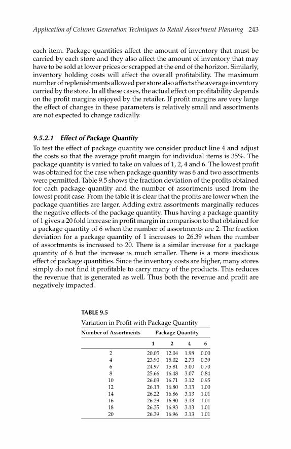
P1: shibu/Vijay

August 10, 2005 11:57 1914 1914˙C009


each item. Package quantities affect the amount of inventory that must becarried by each store and they also affect the amount of inventory that mayhave to be sold at lower prices or scrapped at the end of the horizon. Similarly,inventory holding costs will affect the overall profitability. The maximumnumber of replenishments allowed per store also affects the average inventorycarried by the store. In all these cases, the actual effect on profitability dependson the profit margins enjoyed by the retailer. If profit margins are very largethe effect of changes in these parameters is relatively small and assortmentsare not expected to change radically.

9.5.2.1 Effect of Package Quantity

To test the effect of package quantity we consider product line 4 and adjustthe costs so that the average profit margin for individual items is 35%. Thepackage quantity is varied to take on values of 1, 2, 4 and 6. The lowest profitwas obtained for the case when package quantity was 6 and two assortmentswere permitted. Table 9.5 shows the fraction deviation of the profits obtainedfor each package quantity and the number of assortments used from thelowest profit case. From the table it is clear that the profits are lower when thepackage quantities are larger. Adding extra assortments marginally reducesthe negative effects of the package quantity. Thus having a package quantityof 1 gives a 20 fold increase in profit margin in comparison to that obtained fora package quantity of 6 when the number of assortments are 2. The fractiondeviation for a package quantity of 1 increases to 26.39 when the numberof assortments is increased to 20. There is a similar increase for a packagequantity of 6 but the increase is much smaller. There is a more insidiouseffect of package quantities. Since the inventory costs are higher, many storessimply do not find it profitable to carry many of the products. This reducesthe revenue that is generated as well. Thus both the revenue and profit arenegatively impacted.

TABLE 9.5

Variation in Profit with Package QuantityNumber of Assortments Package Quantity

1 2 4 6

2 20.05 12.04 1.98 0.004 23.90 15.02 2.73 0.396 24.97 15.81 3.00 0.708 25.66 16.48 3.07 0.84

10 26.03 16.71 3.12 0.9512 26.13 16.80 3.13 1.0014 26.22 16.86 3.13 1.0116 26.29 16.90 3.13 1.0118 26.35 16.93 3.13 1.0120 26.39 16.96 3.13 1.01

P1: shibu/Vijay

August 10, 2005 11:57 1914 1914˙C009


0

5

10

15

20

25

30

35

40

1 2 4 6

Package quantity

Pro

fit

(x $

100,

000)

Margin 135%Margin 60%Margin 35%

FIGURE 9.1Effect of package quantity.

Figure 9.1 shows the effect of package quantities as the profit margin ischanged. A more significant effect of package quantities occurs when theprofit margin is higher because more items get included in the assortment.Many more items are therefore affected by the increased package quantity.Since fewer items are carried by the stores for lower margins the effect issomewhat less pronounced even though the extra inventory holding cost hasa more sizeable effect on the profits.

9.5.2.2 Effect of Number of Replenishments

The number of replenishments also affects the inventory holding cost. Themore frequently replenishments are done the less the inventory that is car-ried. Table 9.6 shows fraction deviation from the lowest value obtained forproduct line 4. In this case we use a package quantity of 1. The number ofreplenishments allowed is varied from 3 to 52. Notice that the profit increaseswith the number of replenishments. However, there are diminishing returnsas the number of replenishments increases beyond a point. This is importantto note since in our model we do not solve for the optimal number of replen-ishments and so do not consider the fixed replenishment cost. Clearly, beyonda certain point having extra replenishments may not be able to overcome thecost of replenishments.

When package quantities are varied with the number of replenishments,the profits in all cases continue to increase with the number of replenish-ments. However package quantities seem to have more of an effect whenthere are fewer replenishments. Figure 9.2 shows a plot of the profits againstthe number of replenishments for a number of different package quantities.

P1: shibu/Vijay

August 10, 2005 11:57 1914 1914˙C009


TABLE 9.6

Variation in Profit with Number of ReplenishmentsNumber of Assortments Number of Replenishments

3 4 7 13 26 52

2 0.00 1.09 2.86 4.39 5.31 5.814 0.23 1.50 3.55 5.37 6.47 7.076 0.26 1.58 3.70 5.65 6.80 7.448 0.26 1.62 3.83 5.82 6.99 7.64

10 0.26 1.64 3.90 5.92 7.13 7.7912 0.26 1.65 3.92 5.94 7.16 7.8314 0.26 1.65 3.93 5.97 7.19 7.8716 0.26 1.66 3.95 5.99 7.22 7.9018 0.26 1.66 3.95 6.00 7.24 7.9220 0.26 1.66 3.96 6.01 7.26 7.94

9.5.2.3 Effect of Inventory Holding Cost

To study the effect of holding cost on overall profitability we consider productline 4 again. However, we simultaneously vary the item costs to get differentprofit margins for the SKUs. We consider a profit margin of 35%, 60% and135%. Table 9.7 shows the results of our test runs in the form of percentdeviations. However, to highlight a number of interesting observations thetable shows in columns 2 through 4 the percent deviation when the holdingcost is decreased from a base of 30 to 20%. In columns 5 through 7 we showthe percent deviation when the holding cost is decreased to 30% from a baseof 40%. Clearly, holding costs affect the solution much more when the profit

20

22

24

26

28

30

32

34

36

38

40

3 4 7 13 52

Number of replenishments

Pro

fit

(x $

100

,000

)

Pkg Qty 1Pkg Qty 2Pkg Qty 4Pkg Qty 6

FIGURE 9.2Effect of replenishments and package quantity.

P1: shibu/Vijay

August 10, 2005 11:57 1914 1914˙C009


TABLE 9.7

Percentage Variation in Profit as Holding CostNumber of Assortments 20% vs. 30% 30% vs. 40%

Percentage Profit Margin

135 60 35 135 60 35

2 1.52 5.62 17.04 1.54 5.65 17.234 1.72 5.89 17.39 1.74 5.92 17.296 1.85 6.06 17.49 1.88 6.05 17.718 2.48 6.34 17.43 1.52 6.32 17.50

10 1.97 6.48 17.45 1.98 6.40 17.5112 1.89 6.60 17.49 1.95 6.54 17.4214 1.98 6.73 17.54 1.99 6.64 17.3716 2.00 6.80 17.58 2.01 6.62 17.3518 2.04 6.16 17.59 2.05 6.53 17.3920 2.10 6.91 17.65 2.11 6.69 17.39

margins are smaller. Thus a 10% increase in holding cost affects the solutionmuch more when the profit margin is 35% (approximately 17% deviation) thanwhen the profit margin is 135% (between 1.52% to 2.11%). This is due to the factthat holding cost has a more significant effect on assortment decisions whenmargins are lower. It is also interesting to observe that number of assortmentsplays a more significant part when the margin is higher. When the marginsare higher and holding costs are lower, more products qualify to be part ofan assortment. Thus allowing more assortments makes it possible to tailorthe assortments to individual store requirements giving higher increases inprofit. When margins are low, very few products qualify at higher holdingcosts and permitting more assortments does not increase profitability sincestores do not care to carry most of the products.

9.5.2.4 Effect of Number of Assortments

The number of assortments permitted across all stores is a major determinantof the profit. Figure 9.3 shows the percent deviation of the profit with thenumber of assortments for all five product lines. In each case the profit with 2assortments is taken as the base line to calculate percent deviations. In all casesincreasing the number of assortments leads to increase in the profit but withdiminishing returns. Indeed in all cases having more than 10 assortmentsdoes not materially affect the profit. A striking feature of Figure 9.3 is thesignificantly higher increase that product line 4 exhibits in comparison withthe other product lines. The reason for this is that product line 4 is a lowvolume line with a large number of SKUs and there are significant differencesbetween the stores. When very few assortments are permitted many storesexperience large losses. As more assortments are permitted stores are ableto find assortments that are more suitable to their sales patterns. This allowssuch stores to pick profitable items and avoid loss making items.

P1: shibu/Vijay

August 10, 2005 11:57 1914 1914˙C009


0

15

30

45

60

75

90

105

2 4 6 8 10 12 14 16 18 20

Number of assortments

Per

cen

tag

e d

iffe

ren

ce in

pro

fit

Line 1Line 2Line 3Line 4Line 5

FIGURE 9.3Effect of number of assortments on profits.

9.5.2.5 Effect of Profit Margin

In much of the discussion thus far, we have mentioned the importance of theaverage profit margin on assortment decisions. We conclude our computa-tional results by looking at a plot of the profit to the profit margin. Figure 9.4shows the variation in profit with profit margin. First notice that the y-axis

11.00

11.50

12.00

12.50

13.00

13.50

14.00

14.50

15.00

15.50

135% 60% 35%

Percentage profit margin

ln(P

rofi

t)

Repln 3

Repln 4

Repln 7

Repln 13

Repln 52

FIGURE 9.4Effect of profit margin.

P1: shibu/Vijay

August 10, 2005 11:57 1914 1914˙C009


has a logarithmic scale. This was done to scale the data so that we could showthe relative importance of number of replenishments with changing profitmargins. As is to be expected decreasing the profit margin leads to decreasedprofits. However, it is interesting to note that there is a much smaller effectof the number of replenishments when the profit margin is larger. This stemsfrom the fact that the extra holding cost is a smaller fraction of the overallcost and, thus, does not make products so unprofitable that they are droppedfrom the assortment.

9.6 Conclusions

In this chapter we present the assortment planning problem. We develop amodel and solution algorithm for the problem when a large retail chain mustlimit the number of different assortments that are used. This requires the prob-lem to be solved simultaneously across all stores in the chain. We show how tomodel constraints on inventory productivity, display space, back room space,and inventory budgets. We present an algorithm based on column genera-tion and provide extensive computational results to show how the algorithmperforms.

References

1. Anderson, E.E. and H.N. Amato., A mathematical model for simul-taneously determining the optimal brand-collection and display-areaallocation, Operations Research, 22(1):13–21, 1974.

2. Bazaraa, M.S., J. Jarvis, and H. Sherali., Linear Programming and NetworkFlows, John Wiley and Sons, Inc., 2nd edition, 1990.

3. Borin, N., P. Farris, and J. Freeland., A model for determining retailproduct category and shelf space allocation, Decision Sciences, 25(3):359–384, 1994.

4. Brijs, T., G. Swinnen, K. Vanhoof, and G. Wets., Using association rulesfor product assortment decisions: A case study, Proceedings of the FifthACM SIGKDD International Conference on Knowledge Discovery and DataMining, San Diego, pages 254–260, 1999.

5. Broniarcyzk, S.M., W.D. Hoyer, and L.M. McAlister., Consumers’ per-ceptions of category assortment: The impact of item reduction, Journalof Marketing Research, 35:166–176, 1998.

6. Bultez, A. and P. Naert., S.H.A.R.P.: shelf allocation for retailer’s profit,Marketing Science, 7:211–231, 1988.

P1: shibu/Vijay

August 10, 2005 11:57 1914 1914˙C009


7. Cairns, J.P., Suppliers, retailers, and shelf space, Journal of Marketing, 26(3):34–36, 1962.

8. Chernev, A., Product assortment and individual decision processes,Journal of Personality and Social Psychology, 85(1):151–162, 2003.

9. Chong, J., T. Ho, and C.S. Tang., A modelling framework for categoryassortment planning, Manufacturing and Service Operations Management,3(3):191–210, 2001.

10. Corstjens, M. and P. Doyle., A model for optimizing retail space alloca-tions, Management Science, 27(7):822–833, 1981.

11. Cox, K.K., The effect of shelf space upon sales of branded products,Journal of Marketing Research, 7:55–58, 1970.

12. Curhan, R.C., The relationship between shelf space and unit sales insupermarkets, Journal of Marketing Research, 9(4):406–412, 1972.

13. Dhruv, G., M. Levy, A. Mehrotra, and A. Sharma., Planning merchandis-ing decisions to account for regional and product assortment differences,Journal of Retailing, 75(3):405–424, 1995.

14. Fox, L.J., An integrated view of assortment management process: thenext frontier for leading retailers, Chain Store Age Executive, 71(11), 62–68, November 1995.

15. Frank, R.E. and W.F. Massy., Shelf position and space effect on sales,Journal of Marketing Research, 7:59–66, 1970.

16. Green, P. and A. Krieger., Models and heuristics for product line selec-tion, Marketing Science, 4:1–19, 1985.

17. Guadagni, P. and J. Little., A logit model of brand choice calibrated onscanner data, Marketing Science, 2(3):203–238, 1983.

18. Hoch, S.J., E.T. Bradlow, and B. Wansink., The variety of an assortment,Marketing Science, 18(4):527–546, 1999.

19. Jayaraman, V., R. Srivastava, and W.C. Benton., A joint optimizationof product variety and ordering approach, Computers and OperationsResearch, 25(7/8):557–566, 1998.

20. Kahn, B. E. and D.R. Lehmann., Modelling choice among assortments,Journal of Retailing, 67(3):274–299, 1991.

21. Kahn, B. E. and L. McAlister., Grocery Revolution: The New Focus on theConsumer, Addison-Wesley Pub. Co, 1997.

22. Koelemeijer, K. and H. Oppewal., Assessing the effects of assortmentand ambience: a choice experimental approach, Journal of Retailing, 75(3):319–345, 1995.

23. Lancaster, K., The economics of product variety: a survey, MarketingScience, 9:189–210, 1990.

24. Larson, P.D. and R.A. DeMarais., Psychic stock: An independent vari-able category of inventory, International Journal of Physical Distributionand Logistics Management, 20(7):28–34, 1990.

25. Stassen, R.E., Mittelstaedt, J.D., and Mittelstaedt, R.A., Assortmentoverlap: its effect on shopping patterns in a retail market when the

P1: shibu/Vijay

August 10, 2005 11:57 1914 1914˙C009


distributions of prices and goods are known, Journal of Retailing, 75:371–396, 1995.

26. Levin, R.I., C.P. McLaughlin, R.P. Lamone, and J.F. Kottas., Production/Operations Management: Contemporary Policy for Managing Operating Sys-tems, McGraw-Hill, N.Y., 1972.

27. Lilien, G.L., P. Kotler, and K.S.P. Moorthy., Marketing Models, Prentice-Hall, N.J., 1992.

28. Lim, A., B. Rodriques, and X. Zhang., Metaheuristics with local searchtechniques for retail shelf-space optimization, Management Science, 50:117–131, 2004.

29. Mahajan, S. and G. Van Ryzin., A theory of retail assortments, WorkingPaper no. 96-07-02 , The Department of Operations and Information Manage-ment, The Wharton School, 1996.

30. Mahajan, S. and G. Van Ryzin., Stocking retail assortments under dy-namic consumer substitution, Operations Research, 49(3):334–351, 2001.

31. Pashigan, P.B., Demand uncertainty and sales: A study of fashion andmarkdown pricing, American Economic Review, 78:936–953, 1988.

32. Rajaram, K., Assortment planning in fashion retailing: methodology,application and analysis, European Journal of Operational Research, 129:186–208, 2001.

33. Schary, P.B. and B.W. Becker., Distribution and final demand: The influ-ence of availability, Mississippi Valley Journal of Business and EconomicsIndustrial Management Review, 8(1):17–26, 1972.

34. Shelby, H. M. and C.M. Miller., The selection and pricing of retail assort-ments: an empirical approach, Journal of Retailing, 75(3):295–318, 1995.

35. Shocker, A.D. and V. Srinivasan., Multi attribute approaches for productconcept evaluation and generation: a critical review, Journal of MarketingResearch, 16:159–180, 1979.

36. Silver, E.A. and R. Peterson., Decision Systems for Inventory Managementand Production Planning, John Wiley and Sons, Inc., 2nd edition, 1985.

37. Simonson, I., The effect of product assortment on buyer preferences,Journal of Retailing, 75(3):347–370, 1995.

38. Smith, S.A. and N. Agrawal., Management of multi-item retail inven-tory systems with demand substitution, Operations Research, 48(1):50–64,2000.

39. Urban, G.L., A mathematical modelling approach to product line deci-sions, Journal of Marketing Research, 6:40–47, 1969.

40. Urban, G.L., PERCEPTOR: A model for product positioning, Manage-ment Science, 21:858–871, 1975.

41. Urban, T.L., A mathematical modelling approach to product line deci-sions, Journal of Retailing, 74(1):15–35, 1998.

42. U.S.Census., Annual Benchmark Report for Retail Trade and Food Services- January 1992 through February 2002, accessed on September 7, 2004.http://www.census.gov/prod/2004pubs/br03-a.pdf, 2004.

43. Whitin, T.M., The Theory of Inventory Management, Princeton UniversityPress, 1957.

P1: shibu/Vijay

August 10, 2005 11:57 1914 1914˙C009


44. Williard Bishop Consulting Ltd. and Information Resources Inc., Varietyor duplication: A process to know where you stand, Report Prepared forthe Food Marketing Institute, 1993.

45. Wolfe, H.B., A model for control of style merchandise, Industrial Man-agement Review, 9(2):69–82, 1968.

46. Yang, M., An efficient algorithm to allocate shelf space, European Journalof Operational Research, 131:107–118, 2001.

47. Yang, M. and W. Chen., A study of shelf space allocation and manage-ment, International Journal of Production Economics, 60-61:309–317, 1999.

48. Zufryden, F.S., A dynamic programming approach for product selec-tion and supermarket shelf-space allocation, Journal of the OperationalResearch Society, 37(4):413–422,1986.

P1: shibu/Vijay

August 10, 2005 11:57 1914 1914˙C009

P1: ShashiAugust 12, 2005 11:38 1914 1914˙C010

10Noncommercial Software for Mixed-IntegerLinear Programming

Jeffrey T. Linderoth and Ted K. Ralphs

CONTENTS

10.1 Introduction . . . . . . . . . . . . . . . . . . . . . . . . . . . . . . 25410.2 Branch and Bound . . . . . . . . . . . . . . . . . . . . . . . . . . . 256

10.2.1 Lower Bounding Methods . . . . . . . . . . . . . . . . . 25810.2.1.1 Logical Preprocessing . . . . . . . . . . . . . . 25810.2.1.2 Valid Inequalities . . . . . . . . . . . . . . . . . 25810.2.1.3 Reduced Cost Tightening . . . . . . . . . . . . 26410.2.1.4 Column Generation . . . . . . . . . . . . . . . 264

10.2.2 Upper Bounding Methods . . . . . . . . . . . . . . . . . 26510.2.3 Branching . . . . . . . . . . . . . . . . . . . . . . . . . . . 26610.2.4 Search Strategy . . . . . . . . . . . . . . . . . . . . . . . . 269

10.3 User Interfaces . . . . . . . . . . . . . . . . . . . . . . . . . . . . . 27010.3.1 Black-Box Solvers . . . . . . . . . . . . . . . . . . . . . . 270

10.3.1.1 Raw File Formats . . . . . . . . . . . . . . . . . 27110.3.1.2 Modeling Languages . . . . . . . . . . . . . . . 271

10.3.2 Callable Libraries . . . . . . . . . . . . . . . . . . . . . . 27210.3.2.1 Open Solver Interface . . . . . . . . . . . . . . 27210.3.2.2 Object-Oriented Interfaces . . . . . . . . . . . . 272

10.3.3 Solver Frameworks . . . . . . . . . . . . . . . . . . . . . 27310.4 MILP Software . . . . . . . . . . . . . . . . . . . . . . . . . . . . . 273

10.4.1 ABACUS . . . . . . . . . . . . . . . . . . . . . . . . . . . 27510.4.1.1 Overview . . . . . . . . . . . . . . . . . . . . . 27510.4.1.2 User Interface . . . . . . . . . . . . . . . . . . . 27610.4.1.3 Algorithm Control . . . . . . . . . . . . . . . . 276

10.4.2 BCP . . . . . . . . . . . . . . . . . . . . . . . . . . . . . . 27710.4.2.1 Overview . . . . . . . . . . . . . . . . . . . . . 27710.4.2.2 User Interface . . . . . . . . . . . . . . . . . . . 27810.4.2.3 Algorithm Control . . . . . . . . . . . . . . . . 278

253

P1: ShashiAugust 12, 2005 11:38 1914 1914˙C010


10.4.3 BonsaiG . . . . . . . . . . . . . . . . . . . . . . . . . . . . 27910.4.3.1 Overview . . . . . . . . . . . . . . . . . . . . . 27910.4.3.2 User Interface and Algorithm Control . . . . . 280

10.4.4 CBC . . . . . . . . . . . . . . . . . . . . . . . . . . . . . . 28010.4.4.1 Overview . . . . . . . . . . . . . . . . . . . . . 28010.4.4.2 User Interface . . . . . . . . . . . . . . . . . . . 28110.4.4.3 Algorithm Control . . . . . . . . . . . . . . . . 281

10.4.5 GLPK . . . . . . . . . . . . . . . . . . . . . . . . . . . . . 28210.4.5.1 Overview . . . . . . . . . . . . . . . . . . . . . 28210.4.5.2 User Interface . . . . . . . . . . . . . . . . . . . 28310.4.5.3 Algorithm Control . . . . . . . . . . . . . . . . 283

10.4.6 lp_ solve . . . . . . . . . . . . . . . . . . . . . . . . . . . . 28310.4.6.1 Overview . . . . . . . . . . . . . . . . . . . . . 28310.4.6.2 User Interface . . . . . . . . . . . . . . . . . . . 28410.4.6.3 Algorithm Control . . . . . . . . . . . . . . . . 284

10.4.7 MINTO . . . . . . . . . . . . . . . . . . . . . . . . . . . . 28410.4.7.1 Overview . . . . . . . . . . . . . . . . . . . . . 28410.4.7.2 User Interface . . . . . . . . . . . . . . . . . . . 28510.4.7.3 Algorithm Control . . . . . . . . . . . . . . . . 285

10.4.8 SYMPHONY . . . . . . . . . . . . . . . . . . . . . . . . . 28610.4.8.1 Overview . . . . . . . . . . . . . . . . . . . . . 28610.4.8.2 User Interface . . . . . . . . . . . . . . . . . . . 28710.4.8.3 Algorithm Control . . . . . . . . . . . . . . . . 287

10.5 Case Studies . . . . . . . . . . . . . . . . . . . . . . . . . . . . . . 28810.5.1 Branch and Cut . . . . . . . . . . . . . . . . . . . . . . . . 28810.5.2 Branch and Price . . . . . . . . . . . . . . . . . . . . . . . 291

10.6 Benchmarking . . . . . . . . . . . . . . . . . . . . . . . . . . . . . 29510.7 Future Trends and Conclusions . . . . . . . . . . . . . . . . . . . 298References . . . . . . . . . . . . . . . . . . . . . . . . . . . . . . . . . . . 300

10.1 Introduction

A mixed-integer linear program (MILP) is a mathematical program with lin-ear constraints in which a specified subset of the variables are required to takeon integer values. Although MILPs are difficult to solve in general, the past tenyears have seen a dramatic increase in the quantity and quality of software —both commercial and noncommercial — designed to solve MILPs. Generallyspeaking, noncommercial MILP software tools cannot match the speed or ro-bustness of their commercial counterparts, but they can provide a viable alter-native for users who cannot afford the sometimes costly commercial offerings.For certain applications, open-source software tools can also be more exten-sible and easier to customize than their commercial counterparts, whose flex-ibility may be limited by the interface that is exposed to the user. Because of

P1: ShashiAugust 12, 2005 11:38 1914 1914˙C010

Noncommercial Software for Mixed-Integer Linear Programming 255

the large number of open-source and noncommercial packages available, itmight be difficult for the casual user to determine which of these tools is thebest fit for a given task. In this chapter, we provide an overview of the fea-tures of the available noncommercial and open source codes, compare selectedalternatives, and illustrate the use of various tools. For an excellent overviewof the major algorithmic components of commercial solvers, especiallyCPLEX, LINDO, and XPRESS, we refer to reader to the paper of Atamturkand Savelsbergh [6].

To formally specify a MILP, let a polyhedron

P = x ∈ Rn | Ax = b, x ≥ 0 (10.1)

be represented in standard form by a constraint matrix A ∈ Qm×n and a right-hand side vector b ∈ Qm. Without loss of generality, we assume that thevariables indexed 1 through p ≤ n are the integer-constrained variables (theinteger variables), so that the feasible region of the MILP isP I = P∩Zp ×Rn−p.In contrast, the variables indexed p + 1 through n are called the continuousvariables. A subset of the integer variables, called binary variables, may addi-tionally be constrained to take on only values in the set 0, 1. We will denotethe set of indices of binary variables by B ⊆ 1, 2, . . . , p. The mixed-integerlinear programming problem is then to compute the optimal value

zIP = minx∈P I

cx, (10.2)

where c ∈ Qn is a vector that defines the objective function. The case in whichall variables are continuous (p = 0) is called a linear program (LP). Associatedwith each MILP is an LP called the LP relaxation, obtained by relaxing theinteger restrictions on the variables. For the remainder of the chapter, we usethis standard notation to refer to the data associated with a given MILP andits LP relaxation.

In what follows, we review the relevant notions from the theory and practiceof integer programming and refer to other sources when necessary for thefull details of the techniques described. This chapter is largely self-contained,though we do assume that the reader is familiar with concepts from the theoryof linear programming (see [18]). We also assume that the reader has at leasta high-level knowledge of both object-oriented and functional programminginterfaces. For an in-depth treatment of the theory of integer programming, wedirect the reader to the works of Schrijver [76], Nemhauser and Wolsey [62],and Wolsey [85].

The chapter is organized as follows. In Section 10.2, we sketch the branch-and-cut algorithm, which is the basic method implemented by the solverswe highlight herein, and we describe in some detail the advanced bound im-provement techniques employed by these solvers. In Section 10.3, we discussthe various categories of MILP software systems and describe how they aretypically used. In Section 10.4, we describe the use and algorithmic featuresof eight different noncommercial MILP software systems: ABACUS, BCP,BonsaiG, CBC, GLPK, lp_solve, MINTO, and SYMPHONY. Section 10.5illustrates the use of two solver frameworks to develop specialized algorithms

P1: ShashiAugust 12, 2005 11:38 1914 1914˙C010


for solving specific MILP problems. In Section 10.6, the six noncommercialsolvers that can be used as “black-box” solvers are benchmarked on a suiteof over 100 MILP instances. We conclude by assessing the current state of theart and trends for the future.

10.2 Branch and Bound

Branch and bound is a broad class of algorithms that is the basis for virtually allmodern software for solving MILPs. Here, we focus specifically on LP-basedbranch and bound, in which LP relaxations of the original problem are solved toobtain bounds on the objective function value of an optimal solution. Roughlyspeaking, branch and bound is a divide and conquer approach that reducesthe original problem to a series of smaller subproblems and then recursivelysolves each subproblem. More formally, recall that P I is the set of feasiblesolutions to a given MILP. Our goal is to determine a least cost member of P I

(or prove P I = ∅). To do so, we first attempt to find a “good” solution x ∈ P I

(called the incumbent) by a heuristic procedure or otherwise. If we succeed,then β = c x serves as an initial upper bound on zIP . If no such solution isfound, then we set β = ∞. We initially consider the entire feasible region P I .In the processing or bounding phase, we solve the LP relaxation minx∈P cxof the original problem in order to obtain a fractional solution x ∈ Rn and alower bound c x on the optimal value zIP . We assume this LP relaxation isbounded, or else the original MILP is itself unbounded.

After solving the LP relaxation, we consider x. If x ∈ P I , then x is an optimalsolution to the MILP. Otherwise, we identify k disjoint polyhedral subsets ofP , P1, . . . , Pk , such that ∪k

i=1Pk ∩ Zp × Rn−p = P I . Each of these subsets

defines a new MILP with the same objective function as the original, called asubproblem. Based on this partitioning of P I , we have

minx∈P I

cx = mini∈1 ... k

(min

x∈Pi ∩Zp×Rn−pcx

), (10.3)

so we have reduced the original MILP to a family of smaller MILPs. Thesubproblems associated with P1, . . . , Pk are called the children of the originalMILP, which is itself called the root subproblem. Similarly, a MILP is called theparent of each of its children. The set of subproblems is commonly associatedwith a tree, called the search tree, in which each node corresponds to a sub-problem and is connected to both its children and its parent. We thereforeuse the term search tree node or simply node interchangeably with the termsubproblem and refer to the original MILP as the root node or root of this tree.

After partitioning, we add the children of the root subproblem to the listof candidate subproblems (those that await processing) and associate with eachcandidate a lower bound either inherited from the parent or computed during

P1: ShashiAugust 12, 2005 11:38 1914 1914˙C010


the partitioning procedure. This process is called branching. To continue thealgorithm, we select one of the candidate subproblems and process it, i.e.,solve the associated LP relaxation to obtain a fractional solution x ∈ Rn, if oneexists. Let the feasible region of the subproblem be S ⊆ P ∩Zp ×Rn−p. Thereare four possible results:

1. If the subproblem has no solutions, then we discard, or fathom it.2. If c x ≥ β, then S cannot contain a solution strictly better than x

and we may again fathom the subproblem.3. If x ∈ S and c x < β, then x ∈ P I and is the best solution found so

far. We set x ← x and β ← c x, and again fathom the subproblem.4. If none of the above three conditions hold, we are forced to branch

and add the children of this subproblem to the list of candidatesubproblems.

We continue selecting subproblems in a prescribed order (called the searchorder) and processing them until the list of candidate subproblems is empty,at which point the current incumbent must be the optimal solution. If noincumbent exists, then P I = ∅.

This procedure can be seen as an iterative scheme for improvement of thedifference between the current upper bound, which is the objective functionvalue of the current incumbent, and the current lower bound, which is theminimum of the lower bounds of the candidate subproblems. The differencebetween these two bounds is called the optimality gap. We will see later thatthere is a tradeoff between improving the upper bound and improving thelower bound during the course of the algorithm.

The above description highlights the four essential elements of a branch-and-bound algorithm:

• Lower bounding method: A method for determining a lower boundon the objective function value of an optimal solution to a givensubproblem.

• Upper bounding method: A method for determining an upper boundon the optimal solution value zIP .

• Branching method: A procedure for partitioning a subproblem to ob-tain two or more children.

• Search strategy: A procedure for determining the search order.

With specific implementations of these elements, many different versions ofthe basic algorithm can be obtained. So far, we have described only the moststraightforward implementation. In the sections that follow, we discuss anumber of the most common improvements to these basic techniques. Furtherimprovements may be possible through exploitation of the structure of aparticular problem class.

P1: ShashiAugust 12, 2005 11:38 1914 1914˙C010


10.2.1 Lower Bounding Methods

The effectiveness of the branch and bound algorithm depends critically onthe ability to compute bounds that are close to the optimal solution value.In an LP-based branch-and-bound algorithm, the lower bound is obtainedby solving an LP relaxation, as we have indicated. There are a number ofways in which this lower bound can be potentially improved using advancedtechniques. In the remainder of this section, we describe those that are imple-mented in the software packages reviewed in Section 10.4.

10.2.1.1 Logical Preprocessing

One method for improving the lower bound that can be applied even beforethe solution algorithm is invoked is logical preprocessing. By application ofsimple logical rules, preprocessing methods attempt to tighten the initial for-mulation and thereby improve the bound that will be produced when the LPrelaxation is solved. Formally, preprocessing techniques attempt to determinea polyhedron R such that P I ⊆ R ⊂ P . The bound obtained by minimizingoverR is still valid but may be better than that obtained by minimizing overP .

Preprocessing techniques are generally limited to incremental improve-ments of the existing constraint system. Although they are frequentlydesigned to be applied to the original formulation before the solution algo-rithm is invoked, they can also be applied to individual subproblems duringthe search process if desired. Preprocessing methods include procedures foridentification of obviously infeasible instances, removal of redundant con-straints, tightening of bounds on variables by analysis of the constraints,improvement of matrix coefficients, and improvement of the right-hand sidevalue of constraints. For example, a constraint

n∑j=1

aijx j ≤ bi

can be replaced by the improved constraint∑

j∈1,...,n\kaijx j + (ak − δ)xk ≤ bi − δ

for k ∈ B such that∑

j∈1,...,n\k aijx j ≤ bi − δ∀x ∈ P I . This technique is calledcoefficient reduction. Another technique, called probing, can be used to deter-mine the logical implications of constraints involving binary variables. Theseimplications are used in a variety of ways, including the generation of validinequalities, as described next in Section 10.2.1.2. An extended discussion ofadvanced preprocessing and probing techniques, can be found in the paperof Savelsbergh [74].

10.2.1.2 Valid Inequalities

The preprocessing concept can be extended by dynamically generating en-tirely new constraints that can be added to the original formulation without

P1: ShashiAugust 12, 2005 11:38 1914 1914˙C010


excluding members of P I . To introduce this concept formally, we define aninequality as a pair (a, a0) consisting of a coefficient vector a ∈ Rn and a right-hand side a0 ∈ R. Any member of the half-space x ∈ Rn | ax ≤ a0 is saidto satisfy the inequality and all other points are said to violate it. An inequalityis valid for P I if all members of P I satisfy it.

A valid inequality (a, a0) is called improving for a given MILP if

mincx | x ∈ P , ax ≤ a0 > mincx | x ∈ P.A necessary and sufficient condition for an inequality to be improving is thatit be violated by all optimal solutions to the LP relaxation, so violation ofthe fractional solution x ∈ Rn generated by solution of the LP relaxation ofa MILP is necessary for a valid inequality to be improving. If a given validinequality violated by x is not improving, adding it to the current LP relaxationwill still result in the generation of a new fractional solution, however, andmight, in turn, result in the generation of additional candidate inequalities.By repeatedly searching for violated valid inequalities and using them toaugment the LP relaxation, the bound may be improved significantly. If suchan iterative scheme for improving the bound is utilized during the processingof each search tree node, the overall method is called branch and cut. Generationof valid inequalities in the root node only is called cut and branch. Branch andcut is the method implemented by the vast majority of solvers today.

Valid inequalities that are necessary to the description of conv(P I) are calledfacet-defining inequalities. Because they provide the closest possible approxi-mation of conv(P I), facet-defining inequalities are typically very effective atimproving the lower bound. They are, however, difficult to generate in gen-eral. For an arbitrary vector x ∈ Rn and polyhedron R ⊆ R

n, the problem ofeither finding a facet-defining inequality (a, a0) violated by x or proving thatx ∈ R is called the facet identification problem. The facet identification problemfor a given polyhedron is polynomially equivalent to optimizing over thesame polyhedron [37], so finding a facet-defining inequality violated by anarbitrary vector is in general as hard as solving the MILP itself. The problem ofgenerating a valid inequality violated by a given fractional solution, whetherfacet-defining or not, is called the separation problem.

To deal with the difficulty of the facet identification problem, a common ap-proach is to generate valid inequalities (possibly facet-defining) for the convexhull of solutions to a relaxation of the instance. In the following paragraphs,we describe commonly arising relaxations of general MILPs and classes ofvalid inequalities that can be derived from them. In most cases, the relaxationscome from substructures that are not present in all MILPs, which means thatthe associated classes of valid inequalities cannot always be generated. Twoexceptions are the Gomory and MIR inequalities, which can be generated forall MILP instances. Most solvers will try to determine automatically whichsubstructures exist and activate the appropriate subroutines for cut genera-tion. However, this is difficult at best. Therefore, if certain substructures areknown not to exist a priori, then it is worthwhile for the user to disable sub-routines that generate the corresponding classes of inequalities. On the other

P1: ShashiAugust 12, 2005 11:38 1914 1914˙C010


hand, if a particular substructure is known to exist, it is worthwhile to seekout a solver that can take advantage of this fact. The classes of valid inequal-ities covered here are those employed by at least one of the noncommercialsolvers that we describe in Section 10.4.

Although subroutines for generating valid inequalities are generally in-tegrated into the solver itself, free-standing subroutines for generating in-equalities valid for generic MILPs can be obtained from the open-source CutGeneration Library (CGL), available for download as part of the Computa-tional Infrastructure for Operations Research (COIN-OR) software suite [19].The library is provided by the COIN-OR Foundation and includes separationroutines for most of the classes of valid inequalities reviewed here. Three ofthe MILP solvers discussed in Section 10.4 make use of generic separationroutines that are part of the CGL.

Knapsack Cover Inequalities. Often, a MILP has a row i of the form∑j∈B

aijx j ≤ bi . (10.4)

We assume without loss of generality that aij > 0 for all j ∈ B (if not, we cancomplement the variables for which aij < 0). Considering only (10.4), we havea relaxation of the MILP, called the 0 − 1 knapsack problem, with the feasibleregion

Pknap =

x ∈ 0, 1B |∑j∈B

aj xj ≤ b

.

Note that in all of the relaxations we consider, the feasible region is implicitlyassumed to be contained in the space Zp ×Rn−p, and the variables not explic-itly present in the relaxation are treated as free. Many researchers have studiedthe structure of the knapsack problem and have derived classes of facet-defining inequalities for it [7, 42, 83].

A set C ⊆ B is called a cover if j∈C aj > b. A cover C is minimal if there doesnot exist a k ∈ C such that C \ k is also a cover. For any cover C , we musthave ∑

j∈C

xj ≤ |C | − 1

for all x ∈ P knap. This class of valid inequalities are called cover inequalities.In general, these inequalities are not facet-defining for P knap, but they canbe strengthened through a procedure called lifting. The interested reader isreferred to the paper by Gu, Nemhauser, and Savelsbergh [40].

GUB Cover Inequalities. A generalized upper bound (GUB) inequality is aninequality of the form

∑j∈Q

xj ≤ 1,

P1: ShashiAugust 12, 2005 11:38 1914 1914˙C010


where Q ⊆ B. When MILP contains a knapsack row i of the form (10.4) and aset of GUB inequalities defined by disjoint sets Qk ⊂ B for k ∈ K , we obtaina relaxation of MILP with the feasible region

P GUB =x ∈ 0, 1B |

∑j∈B

aijx j ≤ bi ,∑j∈Qk

xj ≤ 1 ∀k ∈ K

.

This class of inequalities models a situation in which a subset of items notviolating the knapsack inequality (10.4) must be selected, and within thatsubset of items, at most one element from each of the subsets Qi can beselected. A GUB cover CG is a cover that obeys the GUB constraints, (i.e., notwo elements of the cover belong to the same Qi ). For any GUB cover CG , theinequality

∑j∈CG

xj ≤ |CG | − 1

is valid for P GUB. Again, a lifting procedure, in this case one that takes intoaccount the GUB constraints, can lead to significant strengthening of theseinequalities. For more details of the inequalities and lifting procedure, see thepaper of Wolsey [84] and the paper of Gu, Nemhauser, and Savelsbergh [38].

Flow Cover Inequalities. Another important type of inequality commonlyfound in MILP problems is a variable upper bound. A variable upper bound isan inequality of the form

xj ≤ Uj xk,

where xj is a continuous variable ( j > p), xk is a binary variable (k ∈ B), andUj is an upper bound on variable xj . Such inequalities model the implicationxk = 0 ⇒ xj = 0. Variable upper bound inequalities are often used to modela fixed charge associated with assignment of a positive value to variable xj ,and they are particularly prevalent in network flow models. In such models,we can often identify a relaxation with the following feasible region:

P flow =

(x1, x2) ∈ Rn′+ × 0, 1n′

∣∣∣∣∣∑j∈N+

x1j

−∑j∈N−

x1j ≤ d, x1

j ≤ Uj x2j , j ∈ N

,

where N+ and N− are appropriate sets of indices, N = N+ ∪ N−, and n′ = |N|.A set C = C+ ∪ C− is called a flow cover if C+ ⊆ N+, C− ⊆ N− and j∈C+mj −

j∈C−m j > d . For any flow cover C , the inequality∑j∈C+

xj +∑

j∈C++(m j − λ)(1 − yj ) ≤ d +

∑j∈C−

m j +∑j∈L−

λyj +∑

j∈L−−xj ,

P1: ShashiAugust 12, 2005 11:38 1914 1914˙C010


where λ = j∈C+m j − j∈C−m j − d, C++ = j ∈ C+ | m j > λ, L− ⊆ (N−\C−)

and m j > λ for j ∈ L−, and L−− = N−\(L− ∪ C−), is called a simple gen-eralized flow cover inequality and is valid for P flow. Just as with knapsackcover inequalities, these inequalities can be strengthened through lifting toobtain an inequality called the lifted simple generalized flow cover inequality. Thefull details of obtaining such inequalities are given by Gu, Nemhauser, andSavelsbergh [39].

Clique Inequalities. Many MILPs contain logical restrictions on pairs of bi-nary variables such as xi = 1 ⇒ xj = 0. In such cases, an auxiliary data struc-ture, called a conflict graph, can be used to capture these logical conditions andfurther exploit them [4]. The conflict graph is a graph with vertex set B, andan edge between each pair of nodes that correspond to a pair of variables thatcannot simultaneously have the value one in any optimal solution. The logicalrestrictions from which the conflict graph is derived may be present explicitlyin the original model (for example, GUB inequalities lead directly to edges inthe conflict graph), or may be discovered during preprocessing (see [5, 74]).

Because any feasible solution x ∈ P I must induce a vertex packing in theconflict graph, inequalities valid for the vertex packing polytope of the conflictgraph are also valid for the MILP instance from which the conflict graph wasderived. Classes of inequalities valid for the vertex packing polytope havebeen studied by a number of authors [17, 43, 63, 65]. As an example, if C isthe set of indices of nodes that form a clique in a conflict graph for a MILPinstance, then the clique inequality∑

j∈C

xj ≤ 1

is satisfied by all x ∈ P I . Alternatively, if O is a cycle in a conflict graph for aMILP instance, and |O| is odd, then the odd-hole inequality

∑j∈O

xj ≤ |O| − 12

is also satisfied by all x ∈ P I . Again, these inequalities can be strengthenedby lifting [63, 64].

Implication Inequalities. In some cases, the logical implications discoveredduring preprocessing are not between pairs of binary variables (in whichcase clique and odd-hole inequalities can be derived), but between a binaryvariable and a continuous variable. These logical implications can be enforcedusing inequalities known as implication inequalities. If xi is a binary variableand xj is a continuous variable with upper bound U, the implication

xi = 0 ⇒ xj ≤ α

yields the implication inequality

xj ≤ α + (U − α)xi .

Other implication inequalities can also be derived. For more details, see thepaper of Savelsbergh [74].

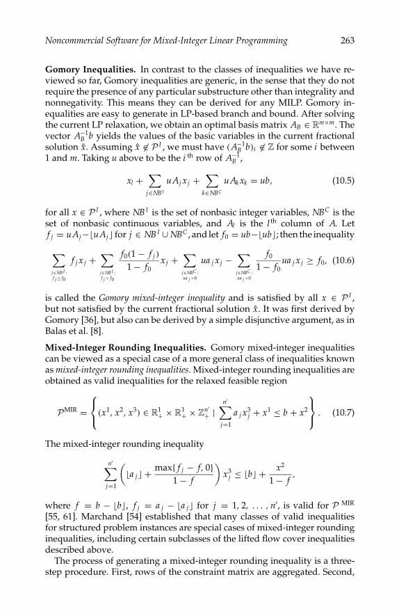
P1: ShashiAugust 12, 2005 11:38 1914 1914˙C010


Gomory Inequalities. In contrast to the classes of inequalities we have re-viewed so far, Gomory inequalities are generic, in the sense that they do notrequire the presence of any particular substructure other than integrality andnonnegativity. This means they can be derived for any MILP. Gomory in-equalities are easy to generate in LP-based branch and bound. After solvingthe current LP relaxation, we obtain an optimal basis matrix AB ∈ Rm×m. Thevector A−1

B b yields the values of the basic variables in the current fractionalsolution x. Assuming x ∈ P I , we must have (A−1

B b)i ∈ Z for some i between1 and m. Taking u above to be the i th row of A−1

B ,

xl +∑

j∈NB I

uAj xj +∑

k∈NBC

uAk xk = ub, (10.5)

for all x ∈ P I , where NB I is the set of nonbasic integer variables, NBC is theset of nonbasic continuous variables, and Al is the l th column of A. Letf j = uAj−uAj for j ∈ NB I ∪ NBC , and let f0 = ub−ub; then the inequality

∑j∈NB I :f j ≤ f0

f j x j +∑j∈NB I :f j > f0

f0(1 − f j )

1 − f0xj +

∑j∈NBC :ua j >0

ua j xj −∑j∈NBC :ua j <0

f0

1 − f0ua j xj ≥ f0, (10.6)

is called the Gomory mixed-integer inequality and is satisfied by all x ∈ P I ,but not satisfied by the current fractional solution x. It was first derived byGomory [36], but also can be derived by a simple disjunctive argument, as inBalas et al. [8].

Mixed-Integer Rounding Inequalities. Gomory mixed-integer inequalitiescan be viewed as a special case of a more general class of inequalities knownas mixed-integer rounding inequalities. Mixed-integer rounding inequalities areobtained as valid inequalities for the relaxed feasible region

PMIR =(x1, x2, x3) ∈ R1

+ × R1+ × Zn′

+ |n′∑

j=1

a j x3j + x1 ≤ b + x2

. (10.7)

The mixed-integer rounding inequality

n′∑j=1

(a j + max f j − f, 0

1 − f

)x3

j ≤ b + x2

1 − f,

where f = b − b, f j = a j − a j for j = 1, 2, . . . , n′, is valid for P MIR

[55, 61]. Marchand [54] established that many classes of valid inequalitiesfor structured problem instances are special cases of mixed-integer roundinginequalities, including certain subclasses of the lifted flow cover inequalitiesdescribed above.

The process of generating a mixed-integer rounding inequality is a three-step procedure. First, rows of the constraint matrix are aggregated. Second,

P1: ShashiAugust 12, 2005 11:38 1914 1914˙C010


bound substitution of the simple or variable upper and lower bounds is per-formed, and variables are complemented to produce a relaxation of the form(10.7). Third, a heuristic separation procedure is used to find mixed-integerrounding inequalities valid for some such relaxation and violated by the cur-rent fractional solution. Marchand and Wolsey [55] discuss the application ofmixed-integer rounding inequalities in detail.

10.2.1.3 Reduced Cost Tightening

After the LP relaxation of MILP is solved, the reduced costs of nonbasic integervariables can be used to tighten bounds on integer variables for the subtreerooted at that node. Although we have assumed a problem given in standardform, upper and lower bounds on variable values are typically present and arehandled implicitly. Such bound constraints take the form l ≤ x ≤ u for l, u ∈ Rn

for all x ∈ P I . Even if no such bound constraints are initially present, they maybe introduced during branching. Let c j be the reduced cost of nonbasic integervariable j , obtained after solution of the LP relaxation of a given subproblemand let x ∈ Rn be an optimal fractional solution. If x j = l j ∈ Z and γ ∈ R+ issuch that c x+γ c j =β, where β is the objective function value of the currentincumbent, then xj ≤ l j +γ in any optimal solution. Hence, we can replacethe previous upper bound u j with min(u j , l j +γ ). The same procedure canbe used to potentially improve the lower bounds. This is an elementary formof preprocessing, but can be very effective when combined with other formsof logical preprocessing, especially when the optimality gap is small. Notethat if this tightening takes place in the root node, it is valid everywhere andcan be considered an improvement of the original model. Some MILP solversstore the reduced costs from the root LP relaxation, and use them to performthis preprocessing whenever a new incumbent is found.

10.2.1.4 Column Generation

A technique for improving the lower bound that can be seen as “dual” to thedynamic generation of valid inequalities is that of column generation. Most col-umn generation algorithms can be viewed as a form of Dantzig-Wolfe decom-position, so we concentrate here on that technique. Consider a relaxation of theoriginal MILP with feasible set F ⊃ P I . We assume that F is finite and that itis possible to effectively optimize overF , but that a minimal description of theconvex hull ofF is of exponential size. LetQ = x ∈ Rn | Dx = d, x ≥ 0 ⊃ P I

be a polyhedron that represents the feasible region of a second relaxationwhose description is “small” and such that F ∩Q ∩ Zp ∩Rn−p = P I . We canthen reformulate the original integer program as

min

∑s∈F

csλs |∑s∈F

(Ds)λs = d, λs 1 = 1, λ ≥ 0, λ ∈ ZF

, (10.8)

where 1 is a vector of all ones of conformable dimension. Relaxing the inte-grality restriction on λ, we obtain a linear program whose optimal solution

P1: ShashiAugust 12, 2005 11:38 1914 1914˙C010


yields the (possibly) improved bound

minx∈F∩Q

cx ≥ minx∈P

cx. (10.9)

Of course, this linear program generally has an exponential number ofcolumns. Therefore, we must generate them dynamically in much the samefashion as valid inequalities are generated in branch and cut. If we solve theabove linear program with a subset of the full set of columns to obtain a dualsolution u, then the problem of finding the column with the smallest reducedcost among those not already present is equivalent to solving

mins∈F

(c − uD)s, (10.10)

which is referred to as the column generation subproblem. Because this is anoptimization problem over the set F , it can be solved effectively, and henceso can the linear program itself. When employed at each search tree nodeduring branch and bound, the overall technique is called branch and price.

Because of the often problem-specific nature of the column generation sub-problem, branch and price is frequently implemented using a solver frame-work. Recently two different groups have undertaken efforts to developgeneric frameworks for performing column generation. Vanderbeck [82] isdeveloping a framework for branch and price that will take care of many ofthe generic algorithmic details and allow the solver to behave essentially as ablack box. Ralphs and Galati (see Chapter 4) have undertaken a similar effortin developing DECOMP, a general framework for computing bounds usingdecomposition within a branch-and-bound procedure. Currently, however,implementing a branch-and-price algorithm is a rather involved procedurethat requires a certain degree of technical expertise. Section 10.5.2 also de-scribes the implementation of a branch-and-price algorithm using the BCPframework.

10.2.2 Upper Bounding Methods

In branch and bound, upper bounds are obtained by discovering feasible solu-tions to the original MILP. Feasible solutions arise naturally if the branch-and-bound algorithm is allowed to run its full course. However, acceleration of theprocess of finding feasible solutions has three potential benefits. First, the so-lution process may be terminated prematurely and in such a case, we wouldlike to come away with a solution as close to optimal as possible. Second,an improved upper bound β may lead to generation of fewer subproblemsbecause of earlier fathoming (depending on the search strategy being em-ployed). Third, a good upper bound allows the bounds on integer variables tobe tightened on the basis of their reduced cost in the current relaxation (see Sec-tion 10.2.1.3). Such tightening can in turn enable additional logical preprocess-ing and may result in significant improvement to the lower bound as a result.

The process of finding feasible solutions during the search procedure canbe accelerated in two ways. The first is to influence the search order, choosing

P1: ShashiAugust 12, 2005 11:38 1914 1914˙C010


to evaluate and partition nodes that are close to being integer feasible. Thistechnique is further discussed in Section 10.2.4. The second is to use a heuristicprocedure, called a primal heuristic, to construct a solution. Primal heuristicsare applied during the search process and generally take an infeasible frac-tional solution as input. A very simple heuristic procedure is to round thefractional components of the infeasible solution in an attempt to produce afeasible solution. The current solution may be rounded in many ways anddetermination of a rounding that maintains feasibility with respect to theconstraints Ax = b may be difficult for certain problem classes. A more so-phisticated class of primal heuristics, called pivot and complement, involvespivoting fractional variables out of the current linear programming basis inorder to achieve integrality [9, 59, 11]. Still other classes of primal heuristicsuse the solution of auxiliary linear programs to construct a solution. One sim-ple, yet effective example of such a heuristic is known as the diving heuristic.In the diving heuristic, some integer variables are fixed and the linear pro-gram resolved. The fixing and resolving is iterated until either an integralsolution is found or the linear program becomes infeasible. Recent successfulprimal heuristics, such as local branching [29] and RINS [22], combine solu-tion of auxiliary linear programs with methods that control the neighborhoodof feasible solutions to be searched.

10.2.3 Branching

Branching is the method by which a MILP is divided into subproblems. InLP-based branch and bound, there are three requirements for the branchingmethod. First, the feasible region must be partitioned in such a way that theresulting subproblems are also MILPs. This means that the subproblems areusually created by imposing additional linear inequalities. Second, the unionof the feasible regions of the subproblems must contain at least one optimalsolution. Third, because the primary goal of branching is to improve theoverall lower bound, it is desirable that the current fractional solution notbe contained in any of the members of the partition. Otherwise, the overalllower bound will not be improved.

Given a fractional solution to the LP relaxation x ∈ Rn, an obvious way

to fulfill the above requirements is to choose an index j < p such that x j ∈ Zand to create two subproblems, one by imposing an upper bound of x j onvariable j and a second by imposing a lower bound of x j. This partitioningis valid because any feasible solution must satisfy one of these two linear con-straints. Furthermore, x is not feasible for either of the resulting subproblems.This partitioning procedure is known as branching on a variable.

Typically, there are many integer variables with fractional values, so wemust have a method for deciding which one to choose. A primary goal ofbranching is to improve the lower bound of the resulting relaxations. Themost straightforward branching methods are those that choose the branch-ing variable based solely on the current fractional solution and do not useany auxiliary information. Branching on the variable with the largest frac-tional part, the first variable (by index) that is fractional, or the last variable

P1: ShashiAugust 12, 2005 11:38 1914 1914˙C010


(by index) that is fractional are examples of such procedures. These rules tendto be too myopic to be effective, so many solvers use more sophisticated ap-proaches. Such approaches fall into two general categories: forward-lookingmethods and backward-looking methods. Both types of methods try to choose thebest partitioning by predicting, for a given candidate partitioning, how muchthe lower bound will actually be improved. Forward-looking methods gener-ate this prediction based solely on locally generated information obtained by“presolving” candidate subproblems. Backward-looking methods take intoaccount the results of previous partitionings to predict the effect of futureones. Of course, as one might expect, hybrids that combine these two basicapproaches also exist [2].

A simple forward-looking method is the penalty method of Driebeek [26],which implicitly performs one dual simplex pivot to generate a lower boundon the bound improvement that could be obtained by branching on a givenvariable. Tomlin [79] improved on this idea by considering the integrality ofthe variables. Strong branching is an extension of this basic concept in whichthe solver explicitly performs a fixed and limited number of dual simplexpivots on the LP relaxations of each of the children that result from branch-ing on a given variable. This is called presolving and again provides a boundon the improvement one might see as a result of a given choice. The effec-tiveness of strong branching was first demonstrated by Applegate et al. intheir work on the traveling salesman problem [3] and has since become amainstay for solving difficult combinatorial problems. An important aspectof strong branching is that presolving a given candidate variable is a relativelyexpensive operation, so it is typically not possible to presolve all candidates.The procedure is therefore usually accomplished in two phases. In the firstphase, a small set of candidates is chosen (usually based on one of the simplemethods described earlier). In the second phase, each of these candidates ispresolved, and the final choice is made using one of the selection rules to bedescribed below.

Backward-looking methods generally depend on the computation of pseu-docosts [14] to maintain a history of the effect of branching on a given variable.Such procedures are based on the notion that each variable may be branchedon multiple times during the search and the effect will be similar each time.Pseudocosts are defined as follows. With each integer variable j , we asso-ciate two quantities, P−

j and P+j , that estimate the per unit increase in objec-

tive function value if we fix variable j to its floor and ceiling, respectively.Suppose that f j = x j − x j > 0. Then by branching on variable j , we willestimate an increase of D−

j = P−j f j on the “down branch” and an increase of

D+j = P+

j (1 − f j ) on the “up branch”.The most important aspect of using pseudocosts is the method of obtaining

the values P−j and P+

j for variable j . A popular way to obtain these valuesis to simply observe and record the true increase in objective function valuewhenever variable j is chosen as the branching variable. For example, if agiven subproblem had lower bound zLP and its children had lower boundsz−

LP and z+LP after branching on variable j, then the pseudocosts would be

P1: ShashiAugust 12, 2005 11:38 1914 1914˙C010


computed as

P−j = z−

LP − zLP

f jP+

j = z+LP − zLP

1 − f j, (10.11)

where f j is the fractional part of the value of variable j in the solution to theLP relaxation of the parent. The pseudocosts may be updated using the firstobservation, the last observation, or by averaging all observations. In contrastto the estimates generated in strong branching, generation of pseudocostestimates is inexpensive, so they are typically calculated for all variables.

Whether using a forward-looking or a backward-looking method, the finalstep is to select the branching variable. The goal is to maximize the improve-ment in the lower bound from the parent to each of its children. Because eachparent has two (or more) children, however, no unique metric exists for thischange. Suggestions in the literature have included maximization of the sumof the changes on both branches [35], maximization of the smaller of the twochanges [12], or a combination of the two [27].

More general methods of branching can be obtained by branching on otherdisjunctions. For any vector a ∈ Z

n whose last n − p entries are zero, wemust have ax ∈ Z for all x ∈ P I . Thus, if a x ∈ Z, a can be used to producea disjunction by imposing the constraint ax ≤ a x in one subproblemand the constraint ax ≥ a x in the other subproblem. This is known asbranching on a hyperplane. Typically, branching on hyperplanes is a problem-specific method that exploits special structure, but it can be made generic bymaintenance of a pool of inequalities that are slack in the current relaxationas branching candidates.

An example of branching on hyperplanes using special structure is GUBbranching. If the MILP contains rows of the form∑

j∈G

xj = 1,

where G ⊆ B, then a valid partitioning is obtained by selection of a nonemptysubset G0 of G, and enforcement of the linear constraint

∑j∈G0 xj = 0 in one

subproblem and the constraint∑

j∈G\G0 xj = 0 in the other subproblem. Theseare linear constraints that partition the set of feasible solutions, and the currentLP solution x is excluded from both resulting subproblems if G0 is chosen sothat 0 ≤∑ j∈G0 x j < 1. GUB branching is a special case of branching on specialordered sets (SOS)1 [13]. Special ordered sets of variables can also be used inthe minimization of separable piecewise-linear nonconvex functions.

Because of their open nature, noncommercial software packages are oftenmore flexible and extensible than their commercial counterparts. This flexibil-ity is perhaps most evident in the array of advanced branching mechanismsthat can be implemented using the open source and noncommercial frame-works we describe in Section 10.4. Using a solver framework with advancedcustomized branching options, it is possible, for instance, to branch directly on

1 Some authors refer to GUBs as special ordered sets of type 1.

P1: ShashiAugust 12, 2005 11:38 1914 1914˙C010


a disjunction, rather than introducing auxiliary integer variables. An impor-tant example of this is in the handling of semicontinuous variables, in whicha variable is constrained to take either the value 0 or a value larger than a pa-rameter K . Additionally, frameworks can make it easy for the user to specifyprioritization schemes for branching on integer variables or to implementcomplex partitioning schemes based on multiple disjunctions.

10.2.4 Search Strategy

As mentioned in Section 10.2.3, branching decisions are made with the goalof improving the lower bound. In selecting the order in which the candidatesubproblems should be processed, however, our focus may be on improvingeither the upper bound, the lower bound, or both. Search strategies, or nodeselection methods, can be categorized as either static methods, estimate-basedmethods, two-phase methods, or hybrid methods.

Static node selection methods employ a fixed rule for selecting the nextsubproblem to process. A popular static method is best-first search, whichchooses the candidate node with the smallest lower bound. Because of thefathoming rule employed in branch and bound, a best-first search strategyensures that no subproblem with a lower bound above the optimal solutionvalue can ever be processed. Therefore, the best-first strategy minimizes thenumber of subproblems processed and improves the lower bound quickly.However, this comes at the price of sacrificing improvements to the upperbound. In fact, the upper bound will only change when an optimal solution islocated. At the other extreme, depth-first search chooses the next candidate to bea node at maximum depth in the tree. In contrast to best-first search, whichwill produce no suboptimal solutions, depth-first search tends to producemany suboptimal solutions, typically early in the search process, because suchsolutions tend to occur deep in the tree. This allows the upper bound to beimproved quickly. Depth-first search also has the advantage that the changein the relaxation being solved from subproblem to subproblem is very slight,so the relaxations tend to solve more quickly when compared to best-firstsearch. Some solvers also allow the search tree to be explored in a breadth-first fashion, but this method offers little advantage over best-first search.

Neither best-first search nor depth-first search make any intelligent at-tempt to select nodes that may lead to improved feasible solutions. Estimate-based methods such as the best-projection method [31, 58] and the best-estimatemethod [14] are improvements in this regard. The best-projection method mea-sures the overall “quality” of a node by combining its lower bound with thedegree of integer infeasibility of the current solution. Alternatively, the best-estimate method combines a node’s lower bound, integer infeasibility, andpseudocost information to rank the desirability of exploring a node.

Because we have two goals in node selection — finding “good” feasiblesolutions (i.e., improving the upper bound) and proving that the current in-cumbent is in fact a “good” solution (i.e., improving the lower bound) — it isnatural to develop node selection strategies that switch from one goal to the

P1: ShashiAugust 12, 2005 11:38 1914 1914˙C010


other during the course of the algorithm. This results in a two-phase searchstrategy. In the first phase, we try to determine “good” feasible solutions,while in the second phase, we are interested in proving this goodness. Perhapsthe simplest “two-phase” algorithm is to perform depth-first search until afeasible solution is found, and then switch to best-first search. A variant ofthis two-phase algorithm is used by many of the noncommercial solvers thatwe describe in Section 10.4.

Hybrid methods also combine two or more node selection methods, butin a different manner. In a typical hybrid method, the search tree is exploredin a depth-first manner until the lower bound of the child subproblem beingexplored rises above a prescribed level in comparison to the overall lower orupper bounds. After this, a new subproblem is selected by a different criterion(e.g., best-first or best-estimate), and the depth-first process is repeated. Foran in-depth discussion of search strategies for mixed-integer programming,see the paper of Linderoth and Savelsbergh [49].

10.3 User Interfaces

An important aspect of the design of software for solving MILPs is the userinterface, which determines both the way in which the user interacts with thesolver and the form in which the MILP instance must be specified. The rangeof purposes for noncommercial MILP software is quite large, so it stands toreason that the number of user interface types is also large. In this section,we broadly categorize the software packages available. The categorizationprovided here is certainly not perfect — some tools fall between categories orinto multiple categories. However, it does represent the most typical ways inwhich software packages for MILP are employed in practice.

10.3.1 Black-Box Solvers

Many users simply want a “black box” that takes a given MILP as inputand returns a solution as output. For such black-box applications, the usertypically interacts with the solver through a command-line interface or aninteractive shell, invoking the solver by passing the name of a file containinga description of the instance to be solved. One of the main differences be-tween various black-box solvers from the user’s perspective is the format inwhich the model can be specified to the solver. In the two sections below, wedescribe two of the most common input mechanisms — raw (uninterpreted)file formats and modeling language (interpreted) file formats. Table 10.1 inSection 10.4 lists the packages covered in this chapter that function as black-box solvers, along with the file formats they accept and modeling languagesthey support. In Section 10.6, we provide computational results that compareall of these solvers over a wide range of instances.

P1: ShashiAugust 12, 2005 11:38 1914 1914˙C010


10.3.1.1 Raw File Formats

One of the first interfaces used for black-box solvers was a standard file formatfor specifying a single instance of a mathematical program. Such a file formatprovides a structured way of constructing a file containing a description ofthe constraint matrix and rim vectors (objective function vector, right handside vector, and variable lower and upper bound vectors) in a form that canbe easily read by the solver. The oldest and most pervasive file format is thelongstanding Mathematical Programming System (MPS) format, developedby IBM in the 1970s. In MPS format, the file is divided into sections, each ofwhich specifies one of the elements of the input, such as the constraint matrix,the right-hand side, the objective function, and upper and lower bounds onthe variables. MPS is a column-oriented format, which means that the con-straint matrix is specified column-by-column in the MPS file. Another popularformat, LP format, is similar to MPS in that the format consists of a text filedivided into different sections, each of which specifies one of the elementsof the input. However, LP format is a row-oriented format, so the constraintmatrix is specified one row at a time in the file. This format tends to be slightlymore readable by humans.

Because MPS was adopted as the de facto standard several decades ago, therehas not been much deviation from this basic approach. MPS, however, is notan easily extensible standard, and is only well-suited for specifying integerand linear models. Several replacements based on the extensible markuplanguage (XML), a wide-ranging standard for portable data interchange, havebeen proposed. One of the most well-developed of these is an open standardcalled LPFML [32]. The biggest advantage of formats based on XML is thatthey are far more extensible and are based on an established standard withbroad support and well-developed tools.

10.3.1.2 Modeling Languages

Despite their wide and persistent use, raw file formats for specifying instanceshave many disadvantages. The files can be tedious to generate, cumbersometo work with, extremely difficult to debug, and are not easily readable byhumans. For these reasons, most users prefer to work with a modeling language.Modeling languages allow the user to specify a model in a more intuitive(e.g., algebraic) format. An interface layer then interprets the model file andtranslates it into a raw format that the underlying solver can interpret directly.Another powerful feature of modeling languages is that they allow for theseparation of the model specification from the instance data.

Full-featured modeling languages are similar to generic programming lan-guages, such as C and C++, in that they have constructs such as loops and con-ditional expressions. They also contain features designed specifically to allowthe user to specify mathematical models in a more natural, human-readableform. Two modeling language systems that are freely available are ZIMPL [87]and GNU Mathprog (GMPL) [53]. ZIMPL is a stand-alone parser that reads ina file format similar to the popular commercial modeling language AMPL [33]

P1: ShashiAugust 12, 2005 11:38 1914 1914˙C010


and outputs the specified math program in either MPS or LP format. GMPLis the GNU Math Programming Language, which is again similar to AMPL.The parser for GMPL is included as part of the GLPK package described inSection 10.4.5, but it can also be used as a free-standing parser.

10.3.2 Callable Libraries

A more flexible mechanism for invoking a MILP solver is through a callablelibrary interface. Most often, callable libraries are still treated essentially as a“black box,” but they can be invoked directly from user code, allowing thedevelopment of custom applications capable of generating a model, invokingthe solver directly without user intervention, parsing the output and inter-preting the results. Callable libraries also make possible the solution of morethan one instance within a single invocation of an application or the use ofthe solver as a subroutine within a larger implementation. The interfaces tothe callable libraries discussed in Section 10.4 are implemented in either C orC++, with each solver generally having its own Application ProgrammingInterface (API). The column labeled Callable API in Table 10.1 of Section 10.4indicates which of the software packages discussed in this chapter havecallable library interfaces and the type of interface available.

The fact that each solver has its own API makes development of portablecode difficult, as this fosters an inherent dependence on one particular API.Recently, however, two open standards for calling solvers have been devel-oped that remove the dependence on a particular solver’s API. These arediscussed below.

10.3.2.1 Open Solver Interface

The Open Solver Interface (OSI), part of the COIN-OR software suite men-tioned earlier, is a standard C++ interface for invoking solvers for LPs andMILPs [51]. The OSI consists of a C++ base class with containers for storinginstance data, as well as a standard set of problem import, export, modifica-tion, solution, and query routines. Each supported solver has a correspondingderived class that implements the methods of the base class and translatesthe standard calls into native calls to the API of the solver in question. Thus,a code that uses only calls from the OSI base class could be easily interfacedwith any supported solver without change. At the time of this writing, elevencommercial and noncommercial solvers with OSI implementations are avail-able, including several of the solvers reviewed in Section 10.4.

10.3.2.2 Object-Oriented Interfaces

In an object-oriented interface, there is a mapping between the mathematicalmodeling objects that comprise a MILP instance (variables, constraints, etc.)and programming language objects. Using this mapping, MILP models canbe easily built in a natural way directly within C++ code. The commercialpackage called Concert Technology [45] by ILOG was perhaps the first ex-ample of such an object-oriented interface. FLOPC++ [44] is an open sourceC++ object-oriented interface for algebraic modeling of LPs and MILPs that

P1: ShashiAugust 12, 2005 11:38 1914 1914˙C010


provides functionality similar to Concert. FLOPC++ allows linear modelsto be specified in a declarative style, similar to algebraic modeling languagessuch as GAMS and AMPL, within a C++ program. As a result, the traditionalstrengths of algebraic modeling languages, such as the ability to declare amodel in a human-readable format, are preserved, while still allowing theuser to embed model generation and solution procedures within a larger ap-plications. To achieve solver independence, FLOPC++ uses the OSI to accessthe underlying solver, and may therefore be linked to any solver with an OSIimplementation. Another interesting interface that allows users to model LPinstances in the python language is PuLP [73].

10.3.3 Solver Frameworks

A solver framework is an implementation of a branch-and-bound, branch-and-cut, or branch-and-price algorithm with hooks that allow the user toprovide custom implementations of certain aspects of the algorithm. For in-stance, the user may wish to provide a custom branching rule or problem-specific valid inequalities. The customization is generally accomplished eitherthrough the use of C language callback functions, or through a C++ inter-face in which the user must derive certain base classes and override defaultimplementations for the desired functions. Some frameworks have the abil-ity to function as black-box solvers, but others, such as BCP and ABACUS,do not include default implementations of certain algorithmic components.Table 10.1 in Section 10.4 indicates the frameworks available and their styleof customization interface.

10.4 MILP Software

In this section, we summarize the features of the noncommercial softwarepackages available for solving MILPs. Table 10.1 to Table 10.3 summarizethe packages reviewed here. In Table 10.1, the columns have the followingmeanings:

• Version Number: The version of the software reviewed for this chap-ter. Note that BCP does not assign version numbers, so we havelisted the date obtained instead.

• LP Solver: The LP software used to solve the relaxations arisingduring the algorithm. The MILP solvers listed as OSI-compliantcan use any LP solver with an OSI interface. ABACUS can use eitherCPLEX, SOPLEX, or XPRESS-MP.

• File Format: The file formats accepted by packages that include ablack-box solver. File formats are discussed in Section 10.3.1.1.

• Callable API: The language in which the callable library interface isimplemented (if the package in question has one). Some packages

P1: ShashiAugust 12, 2005 11:38 1914 1914˙C010


support more than one interface. Two of the solvers, SYMPHONYand GLPK, can also be called through their own OSI implementation.

• Framework API: For those packages that are considered frameworks,this indicates how the callback functions must be implemented —through a C or a C++ interface.

• User’s Manual: Indicates whether the package has a user’s manual.

TABLE 10.1

List of Solvers and Main FeaturesVersion LP Callable Framework User’sNumber Solver File Format API API Manual

ABACUS 2.3 C/S/X no none C++ yesBCP 11/1/04 OSI no none C++ yesbonsaiG 2.8 DYLP MPS none none yesCBC 0.70 OSI MPS C++/C C++ noGLPK 4.2 GLPK MPS/GMPL OSI/C none yeslp_solve 5.1 lp_solve MPS/LP/GMPL C/VB/Java none yesMINTO 3.1 OSI MPS/AMPL none C yesSYMPHONY 5.0 OSI MPS/GMPL OSI/C C yes

Table 10.2 indicates the algorithmic features of each solver, includingwhether the solver has a preprocessor, whether it can dynamically gener-ate valid inequalities, whether it can perform column generation, whetherit includes primal heuristics, and what branching and search strategies areavailable. For the column that indicates available branching methods, theletters stand for the following methods:

• e: pseudocost branching• f: branching on the variables with the largest fractional part• h: branching on hyperplanes• g: GUB branching

TABLE 10.2

Algorithmic Features of SolversBuilt-in Cut Column Primal Branching Search

Preproc Generation Generation Heuristic Rules Strategy

ABACUS no no yes no f,h,s b,r,d,2(d,b)BCP no no yes no f,h,s h(d,b)bonsaiG no no no no p h(d,b)CBC yes yes no yes e,f,g,h,s,x 2(d,p)GLPK no no no no i,p b,d,plp_solve no no no no e,f,i,x d,r,e,2(d,r)MINTO yes yes yes yes e,f,g,p,s b,d,e,h(d,e)SYMPHONY no yes yes no e,f,h,p,s b,r,d,h(d,b)

P1: ShashiAugust 12, 2005 11:38 1914 1914˙C010


• i: branching on first or last fractional variable (by index)• p: penalty method• s: strong branching• x: SOS(2) branching and branching on semicontinuous variables

For the column that indicates available search strategies, the codes stand forthe following:

• b: best-first• d: depth-first• e: best-estimate• p: best-projection• r: breadth-first• h(x,z): a hybrid method switching from strategy ‘x’ to strategy ‘z’• 2(x,z): a two-phase method switching from strategy ‘x’ to strategy ‘z’

Finally, Table 10.3 indicates the classes of valid inequalities generated by thosesolvers that generate valid inequalities.

In the following sections, we provide an overview of each solver, thendescribe the user interface, and finally describe the features of the underly-ing algorithm in terms of the four categories listed in Section 10.2. In whatfollows, the reader should keep in mind that solver performance can varysignificantly with different parameter settings, and it is unlikely that one setof parameters will work best for all classes of MILP instances. When decidingon a MILP package to use, users are well-advised to consider the ability ofa packages to meet their performance requirements through customizationand parameter tuning. An additional caveat about performance is that MILPsolver performance can be affected significantly by the speed with which theLP relaxations are solved, so users may need to pay special attention to theparameter tuning of the underlying LP solver as well.

TABLE 10.3

Classes of Valid Inequalities Generated by Black-Box SolversName Knapsack GUB Flow Clique Implication Gomory MIR

CBC yes no yes yes yes yes yesMINTO yes yes yes yes yes no noSYMPHONY yes no yes yes yes yes yes

10.4.1 ABACUS

10.4.1.1 Overview

ABACUS [46] is a pure solver framework written in C++. It has a flexible,object-oriented design that supports the implementation of a wide variety ofsophisticated and powerful variants of branch and bound. The object-oriented

P1: ShashiAugust 12, 2005 11:38 1914 1914˙C010


design of the library is similar in concept to BCP, described below. From theuser’s perspective, the framework is centered around C++ objects that rep-resent the basic building blocks of a mathematical model — constraints andvariables. The user can dynamically generate variables and valid inequalitiesby defining classes derived from the library’s base classes. ABACUS supportsthe simultaneous generation of variables and valid inequalities for users re-quiring this level of sophistication. Another notable feature of ABACUS is itsvery general implementation of object pools for storing previously generatedconstraints and variables for later use.

ABACUS was a commercial code for some time, but has recently beenreleased under the open source [78] GNU Library General Public License(LGPL). Because of the generality of its treatment of dynamically generatedclasses of constraints and variables, it is one of the most full-featured solverframeworks available. ABACUS does not, however, have a callable libraryinterface and it cannot be used as a black-box solver, though it can be calledrecursively. It comes with complete documentation and a tutorial that showshow to use the code. Compared to the similar MILP framework BCP, ABACUShas a somewhat cleaner interface, with fewer classes and a more straightfor-ward object-oriented structure. The target audience for ABACUS consists ofsophisticated users who need a powerful framework for implementing ad-vanced versions of branch and bound, but who do not need a callable libraryinterface.

10.4.1.2 User Interface

There are four main C++ base classes from which the user may deriveproblem-specific implementations in order to develop a custom solver. Thebase classes are the following:

• ABA_VARIABLE: The base class for defining problem-specific classesof variables.

• ABA_CONSTRAINT: The base class for defining problem-specific classesof constraints.

• ABA_MASTER: The base class for storing problem data and initializingthe root node.

• ABA_SUB: The base class for methods related to the processing of asearch tree node.

In addition to defining new template classes of constraints and variables, thelatter two C++ classes are used to implement various user callback routinesto further customize the algorithm. The methods that can be implemented inthese classes are similar to those in other solver frameworks and can be usedto customize most aspects of the underlying algorithm.

10.4.1.3 Algorithm Control

ABACUS does not contain built-in routines for generating valid inequalities,but the user can implement any desirable separation or column generation

P1: ShashiAugust 12, 2005 11:38 1914 1914˙C010


procedures to improve the lower bound in each search tree node. ABACUSdoes not have a default primal heuristic for improving the upper bound either,but again, the user can implement one easily. ABACUS has a general notion ofbranching in which one may branch on either a variable or a constraint (hy-perplane). Several strategies for selecting a branching variable are provided.In addition, a strong branching facility is provided, in which a number of vari-ables or constraints are selected and presolved before the final branching isperformed. To select the candidates, a sophisticated mechanism for selectionand ranking of candidates using multiple user-defined branching rules is em-ployed. The search strategies include depth-first, breadth-first, and best-firstsearch, as well as a strategy that switches from depth-first to best-first afterthe first feasible solution is found.

10.4.2 BCP

10.4.2.1 Overview

BCP is a pure solver framework developed by Ladanyi [48]. It is a close relativeof SYMPHONY, described below. Both frameworks are descended from theearlier COMPSys framework of Ralphs and Ladanyi [47, 68] like ABACUS.BCP is implemented in C++ and is design centered around problem-specifictemplate classes of cuts and variables, but it takes a more “function-oriented”approach that is similar to SYMPHONY. The design is very flexible and sup-ports the implementation of the same range of sophisticated variants of branchand bound that ABACUS supports, including simultaneous generation ofcolumns and valid inequalities. BCP is a pure solver framework and doesnot have a callable library interface. The BCP library provides its own mainfunction, which means that it cannot easily be called recursively or as a sub-routine from another code. Nonetheless, it is still one of the most full-featuredsolver frameworks available, because of the generality with which it handlesconstraint and variable generation, as well as branching.

Although BCP is not itself a black-box solver, two different black-box codes[56] have been built using BCP and are available along with BCP itself as partof the COIN-OR software suite [48]. BCP is open source software licensedunder the Common Public License (CPL). It has a user’s manual, though it isslightly out of date. The code itself contains documentation that can be parsedand formatted using the Doxygen automatic documentation system [81]. Anumber of applications built using BCP are available for download, includingsome simple examples that illustrate its use. Tutorials developed by Galatithat describe the implementation of two problem-specific solvers — one im-plementing branch and cut and one implementing branch and price — are alsoavailable [34]. The target audience for BCP is similar to that of ABACUS —sophisticated users who need a powerful framework for implementing ad-vanced versions of branch and bound without a callable library interface.BCP is also capable of solving MILPs in parallel and is targeted at users whoneed such a capability.

P1: ShashiAugust 12, 2005 11:38 1914 1914˙C010



To use BCP, the user must implement application-specific C++ classes de-rived from the virtual base classes provided as part of the BCP library. Theclasses that must be implemented fall broadly into two categories: modelingobject classes, which describe the variables and constraints associated with theuser’s application, and user callback classes, which control the execution ofvarious specific parts of the algorithm.

From the user’s point of view, a subproblem in BCP consists primarily of acore relaxation present in every subproblem and a set of modeling objects — theextra constraints and variables that augment the core relaxation. To define newtemplate classes of valid inequalities and variables, the user must derive fromthe classes BCP_cut and BCP_var. The derivation involves defining an ab-stract data structure for describing a member of the class and providing meth-ods for expanding each object (i.e., adding the object to a given LP relaxation).

To enable parallel execution, the internal library and the set of user callbackfunctions are divided along functional lines into five separate computationalmodules. The modular implementation facilitates code maintenance and al-lows easy, configurable parallelization. The five modules are master, tree man-ager, node processor, cut generator, and variable generator. The master moduleincludes functions that perform problem initialization, input/output, andoverall execution control. The tree manager is responsible for maintainingthe search tree and managing the search process. The node processor is re-sponsible for processing a single search tree node (i.e., producing a boundon the solution value of the corresponding subproblem by solving a dynam-ically generated LP relaxation). Finally, the cut and variable generators areresponsible for generating new modeling objects for inclusion in the currentLP relaxation.

Associated with each module “xx” is a class named BCP_xx_user thatcontains the user callbacks for the module. For each module, the user mustimplement a derived class that overrides those methods for which the userwishes to provide a customized implementation. Most, but not all, methodshave default implementations. The user callback classes can also be used tostore the data needed to execute the methods in the class. Such data couldinclude the original input data, problem parameters, and instance-specificauxiliary information such as graph data structures.


Like ABACUS, BCP does not contain built-in routines for generating validinequalities, but the user can implement any separation or column generationprocedure that is desired in order to improve the lower bound. BCP tightensvariable bounds on the basis of reduced cost and allows the user to tightenbounds on the basis of logical implications that arise from the model. BCPdoes not yet have a built-in integer preprocessor and also has no built-inprimal heuristic to improve the upper bound. The user can, however, passan initial upper bound if desired. The default search strategy is a hybriddepth-first/best-first approach in which one of the children of the current

P1: ShashiAugust 12, 2005 11:38 1914 1914˙C010


node is retained for processing as long as the lower bound is not more than aspecified percentage higher than the best available. The user can also specifya customized search strategy by implementing a new comparison functionfor sorting the list of candidate nodes in the BCP_tm_user class.

BCP has a generalized branching mechanism in which the user can specifybranching sets that consist of any number of hyperplanes and variables. Thehyperplanes and variables in these branching sets do not have to be presentin the current subproblem. In other words, one can branch on any arbitraryhyperplane (see Section 10.2.3), whether or not it corresponds to a knownvalid inequality. After the desired candidate branching sets have been cho-sen, each one is presolved as usual by performance of a specified number ofsimplex pivots to estimate the bound improvement that would result fromthe branching. The final branching candidate can then be chosen by a numberof standard built-in rules. The default rule is to select a candidate for whichthe smallest lower bound among its children is maximized.

10.4.3 BonsaiG

10.4.3.1 Overview

BonsaiG is a pure black-box solver developed by Lou Hafer that comes withcomplete documentation and descriptions of its algorithms and is available asopen source software under the GNU General Public License (GPL) [41]. Bon-saiG does not have a documented callable library interface or the customiza-tion options associated with a solver framework. It does, however, have twounique features worthy of mention. The first is the use of a partial arc consis-tency algorithm proposed in [77] to help enforce integrality constraints anddynamically tighten bounds on variables. Although the approach is similarto that taken by today’s integer programming preprocessors, the arc consis-tency algorithm can be seen as a constraint programming technique and isapplied aggressively during the processing of each subproblem. From thisperspective, bonsaiG is perhaps one of the earliest examples of integratingconstraint programming techniques into an LP-based branch-and-bound al-gorithm. The integration of constraint programming and traditional math-ematical programming techniques has recently become a topic of increasedinterest among researchers. Achterberg is currently developing a solver calledSCIP that will also integrate these two approaches [1].

The second feature worthy of mention is the use of DYLP, an implementa-tion of the dynamic LP algorithm of Padberg [66], as the underlying LP solver.DYLP was designed specifically to be used for solving the LP relaxations aris-ing in LP-based branch and bound. As such, DYLP automatically selects thesubsets of the constraints and variables that should be active in a relaxationand manages the process of dynamically updating the active constraints andvariables as the problem is solved. This management must be performed insome fashion by all MILP solvers, but it can be handled more efficiently if keptinternal to the LP solver. The target audience for bonsaiG consists of userswho need a lightweight black-box solver capable of solving relatively small

P1: ShashiAugust 12, 2005 11:38 1914 1914˙C010


MILPs without incurring the overhead associated with advanced boundingtechniques and those who do not need a callable library interface.

10.4.3.2 User Interface and Algorithm Control

BonsaiG can only be called from the command-line, with instances specifiedin MPS format. Algorithm control in bonsaiG is accomplished through the set-ting of parameters that are specified in a separate file. To improve the lowerbound for generic MILPs, bonsaiG aggressively applies the arc consistencyalgorithm discussed earlier in combination with reduced-cost tightening ofbounds in an iterative loop called the integrated variable forcing loop. No gen-eration of valid inequalities or columns is supported. BonsaiG does not haveany facility for improving the upper bound. The default search strategy is ahybrid of depth-first and best-first, but with a slight modification. When a sub-problem is partitioned, all children are fully processed and among those thatare not fathomed, the best one, according to an evaluation function that takesinto account both the lower bound and the integer infeasibility, is retainedfor further partitioning. The others are added to the list of candidates, so thatthe list is actually one of candidates for branching, rather than for processing.When all children of the current node can be fathomed, then the candidatewith the best bound is retrieved from the list and another depth-first searchis initiated.

For branching, BonsaiG uses a penalty method strengthened by integral-ity considerations. Only branching on variables or groups of variables issupported. The user can influence branching decisions for a particular in-stance or develop custom branching strategies through two different mecha-nisms. First, bonsaiG makes the specification of relative branching prioritiesfor groups of variables easy. This tells the solver which variables the userthinks will have the most effect if branched upon. The solver then attemptsto branch on the highest-priority fractional variables first. The second mech-anism is for specifying tours of variables. Tours are groups of variables thatshould be branched on as a whole. The group of child subproblems (called atour group) is generated by adjustment of the bounds of each variable in thetour so that the feasible region of the parent is contained in the union of thefeasible regions of the children, as usual.

10.4.4 CBC

10.4.4.1 Overview

CBC is a black-box solver distributed as part of the COIN-OR softwaresuite [30]. CBC was originally developed by John Forrest as a lightweightbranch-and-cut code to test CLP, the COIN-OR LP solver. However, CBC hassince evolved significantly and is now quite sophisticated, even sporting cus-tomization features that allow it to be considered a solver framework. CBChas a native C++ callable library API similar to the Open Solver Interface,as well as a C interface built on top of that native interface. The CBC solverframework consists of a collection of C++ classes whose methods can be

P1: ShashiAugust 12, 2005 11:38 1914 1914˙C010


overridden to customize the algorithm. CBC does not have a user’s manual,but it does come with some well-commented examples and the source code isalso well-commented. It is distributed as part of the COIN-OR software suiteand is licensed as open source software under the Common Public License(CPL). The target audience for CBC consists of users who need a full-featuredblack-box solver with a callable library API and very flexible, yet relativelylightweight, customization options.


The user interacts with CBC as a black-box solver either by invoking the solveron the command line or through a command-based interactive shell. In eithercase, instances must be specified in MPS format. The callable library API isa hybrid of the API of the underlying LP solver, which is accessed throughthe Open Solver Interface, and the methods in the CbcModel class. To load amodel into CBC, the user creates an OSI object, loads the model into the OSIobject and then passes a pointer to that object to the constructor for the Cbc-Model object. CBC uses the OSI object as its LP solver during the algorithm.

To use CBC as a solver framework, a number of classes can be reimple-mented in order to arrive at a problem-specific version of the basic algorithm.The main classes in the CBC library are:

• CbcObject, CbcBranchingObject, and CbcBranchDecision:The classes used to specify new branching rules. CBC has a verygeneral notion of branching that is similar to that of BCP. CBC’sbranching mechanism is described in more detail in Section 10.4.4.3.

• CbcCompare and CbcCompareBase: The classes used to specifynew search strategies by specifying the method for sorting the listof candidate search tree nodes.

• CbcHeuristic: The class used to specify new primal heuristics.• CbcCutGenerator: The class that interfaces to the Cut Generation

Library.

As seen from the above list, custom branching rules, custom search strategies,custom primal heuristics, and custom generators for valid inequalities can allbe introduced. Cut generator objects must be derived from the Cut GenerationLibrary base class and are created by the user before they are passed to CBC.Primal heuristic objects are derived from the CbcHeuristic class and arealso created before being passed to CBC.


CBC is one of the most full-featured black-box solver of those reviewed herein terms of available techniques for improving bounds. The lower bound canbe improved through the generation of valid inequalities using all of the sep-aration algorithms implemented in the CGL. Problem-specific methods forgeneration of valid inequalities can be implemented, but column generationis not supported. CBC has a logical preprocessor to improve the initial model

P1: ShashiAugust 12, 2005 11:38 1914 1914˙C010


and tightens variable bounds using reduced cost information. Several pri-mal heuristics to improve the upper bound are implemented and providedas part of the distribution, including a rounding heuristic and two differ-ent local search heuristics. The default search strategy in CBC is to performdepth-first search until the first feasible solution is found and then to selectnodes for evaluation on the basis of a combination of bound and number ofunsatisfied integer variables. Specification of new search strategies can alsobe accomplished easily.

CBC has a strong branching mechanism similar to that of other solvers,but the type of branching that can be done is more general. An abstract CBCbranching object can be anything that (1) has a feasible region whose degreeof infeasibility with respect to the current solution can be quantified, (2) hasan associated action that can be taken to improve the degree of infeasibilityin the child nodes, and (3) supports some comparison of the effect of branch-ing. Specification of a CBC branching object involves implementation of threemethods:infeasibility(),feasibleRegion(), andcreateBranch().These methods allow CBC to perform strong branching on any sort of branch-ing objects. Default implementations are provided for branching on integervariables, branching on cliques, and branching on special ordered sets.

10.4.5 GLPK

10.4.5.1 Overview

GLPK is the GNU Linear Programming Kit, a set of subroutines that com-prise a callable library and black-box solver for solving linear programmingand MILP instances [53]. GLPK also comes equipped with GNU MathProg(GMPL), an algebraic modeling language similar to AMPL. GLPK was de-veloped by Andrew Makhorin and is distributed as part of the GNU Project,under the GNU General Public License (GPL). Because GLPK is distributedthrough the Free Software Foundation (FSF), it closely follows the guidelinesof the FSF with respect to documentation and automatic build tools. The buildsystem relies on autoconf, which ensures that users can easily build and ex-ecute the library on a wide variety of platforms. The documentation consistsof a reference manual and a description of the GNU MathProg language. Thedistribution includes examples of the use of the callable library, and modelsdemonstrate the MathProg language.

GLPK is a completely self-contained package that does not rely on exter-nal components to perform any part of the branch-and-bound algorithm. Inparticular, GLPK includes the following main components:

• revised primal and dual simplex methods for linear programming• a primal-dual interior point method for linear programming• a branch-and-bound method• a parser for GNU MathProg• an application program interface (API)• a black-box LP/MILP solver

P1: ShashiAugust 12, 2005 11:38 1914 1914˙C010


The target audience for GLPK consists of users who want a lightweight, self-contained MILP solver with both a callable library and modeling languageinterface.


The default build of GLPK yields the callable library and a black-box solver.The callable library consists of nearly 100 routines for loading and modifyinga problem instance, solving the loaded instance, querying the solver, and get-ting and setting algorithm parameters. There are also utility routines to readand write files in MPS format, LP format, and GMPL format. The subroutinesoperate on a data structure for storing the problem instance that is passedexplicitly, so the code is thread safe and it is possible to work on multiplemodels simultaneously.


Because GLPK was first and foremost developed as a solver of linear pro-grams, it does not yet contain advanced techniques for improving the lowerbound, such as those for preprocessing and generating valid inequalities. Italso does not include a primal heuristic for improving the upper bound. Theuser can set a parameter (either through the callable library or in the black-boxsolver) to choose from one of three methods for selecting a branching variable— the index of the first fractional variable, the index of the last fractional vari-able, or the penalty method discussed in Section 10.2.3. The user can changethe search strategy to either depth-first-search, breadth-first-search, or thebest-projection method described in Section 10.2.4.

10.4.6 lp_solve

10.4.6.1 Overview

Lp_solve is a black-box solver and callable library for linear and mixed-integerprogramming. The original solver was developed by Michel Berkelaar atEindhoven University of Technology, and the work continued with JeroenDirks, who contributed a procedural interface, a built-in MPS reader, andfixes and enhancements to the code. Kjell Eikland and Peter Notebaert tookover development starting with version 4. There is currently an active group ofusers. The most recent version bears little resemblance to earlier versions andincludes a number of unique features, such as a modular LP basis factoriza-tion engine and a large number of language interfaces. Lp_solve is distributedas open source under the GNU Library General Public License (LGPL). Themain repository for lp_solve information, including a FAQ, examples, the fullsource, precompiled executables, and a message board, is available at theYAHOO lp_solve group [15]. The target audience for lp_solve is similar tothat of GLPK — users who want a lightweight, self-contained solver witha callable library API implemented in a number of popular programminglanguages, including C, VB, and Java, as well as an AMPL interface.

P1: ShashiAugust 12, 2005 11:38 1914 1914˙C010



Lp_solve can be used as a black-box solver or as a callable library throughits native C API. The lp_solve API consists of over 200 functions for readingand writing problem instances, building or querying problem instances, set-ting algorithm parameters, invoking solution algorithms, and querying theresults. The lp_solve API has methods that can read and write MPS files, LPformat files, and an XLI (External Language Interface) that allows users toimplement their own readers and writers. At present, XLI interfaces are inplace for GNU MathProg, LPFML, and for the commercial LP formats ofCPLEX and LINDO. An interface to ZIMPL will be available in lp_solve v5.2.

Of the noncommercial MILP software reviewed here, lp_solve has inter-faces to the largest number of different programming languages. Withlp_solve, there are examples that illustrate how to call its API from withina VB.NET or C# program. Also, a Delphi library and a Java Native Interface(JNI) to lp_solve, are available, so lp_solve can be called directly from Javaprograms. AMPL, MATLAB, R, S-Plus, and Excel driver programs are alsoavailable. Lp_solve supports several types of user callbacks and an object-likefacility for revealing functionality to external programs.


Lp_solve does not have any special procedures for improving the upper orlower bounds. Users can set parameters either from the command line orthrough the API to control the branch-and-bound procedure. The search strat-egy is one of depth-first search, breadth-first search, or a two-phase methodthat initially proceeds depth-first, followed by breadth-first. Lp_solve con-tains a large number of built-in branching procedures and can select thebranching variable on the basis of the lowest indexed noninteger column (de-fault), the distance from the current bounds, the largest current bound, themost fractional value, the simple, unweighted pseudocost of a variable, orpseudocosts combined with the number of integer infeasibilities.

The algorithm also allows for GUB branching and for branching on semi-continuous variables (variables that have to take a value of zero or a positivevalue above some given lower bound). The branching rule and search strategyused by lp_solve are set through a call to set_bb_rule(), and the branchingrule can even be modified using parameter values beyond those listed here. Aswith many solvers, MILP performance can be expected to vary significantlybased on parameter settings and model class. The default settings in lp_solveare inherited from v3.2, and tuning is therefore necessary to achieve desirableresults. The developers have indicated that MILP performance improvementand more robust default settings will be a focus in lp_solve v5.3.

10.4.7 MINTO

10.4.7.1 Overview

MINTO (Mixed INTeger Optimizer) is a black-box solver and solver frame-work whose chief architects were George Nemhauser and Martin Savelsbergh,

P1: ShashiAugust 12, 2005 11:38 1914 1914˙C010


with a majority of the software development done by Savelsbergh. MINTOwas developed at the Georgia Institute of Technology and is available inbinary form under terms of an agreement created by the Georgia Tech Re-search Institute. The current maintainer of MINTO is Jeff Linderoth of LehighUniversity. It is available as a precompiled library for a number of commonplatforms [60]. MINTO relies on external software to solve the linear program-ming relaxations that arise during the algorithm. Since version 3.1, MINTOhas been equipped to use the OSI, so any of the linear programming solversfor which there is an OSI interface can be used with MINTO. MINTO canalso be built to directly use the commercial LP solvers CPLEX, XPRESS-MP,and OSL. MINTO comes with a user’s manual that contains instructions forbuilding an executable, and a description of the API for user callbacks thatallow it to be used as a solver framework, and examples of the use of eachroutine. The target audience for MINTO are users who require the powerof a sophisticated solver framework for implementing advanced versions ofbranch and bound, but with a relatively simple C-style interface, or who needa full-featured black-box solver without a callable API.


MINTO can be accessed as a black-box solver from the command line withparameters set through a number of command-line switches. The most com-mon way of using MINTO is to pass problem instances in MPS file format.However, beginning with version 3.1, MINTO can also be used directly withthe AMPL modeling language. MINTO can be customized through the useof “user application” functions (callback functions) that allow MINTO to op-erate as a solver framework. At well-defined points of the branch-and-cutalgorithm, MINTO will call the user application functions, and the user mustreturn a value that signals to MINTO whether or not the algorithm is to bemodified from the default. For example, consider the MINTO user applicationfunction appl_constraints(), which is used for generating user-definedclasses of valid inequalities. The input to appl_constraints() is the solu-tion to the current LP relaxation. The outputs are arrays describing any validinequalities that the user wishes to have added to the formulation. The returnvalue from appl_constraint() should be SUCCESS or FAILURE, depend-ing on whether or not the user-supplied routine was able to find inequalitiesviolated by the input solution. If so, MINTO will add these inequalities andpass the new formulation to the linear programming solver.


To strengthen the lower bound during the course of the algorithm, MINTOrelies on advanced preprocessing and probing techniques, as detailed in thepaper of Atamturk, Nemhauser, and Savelsbergh [5], and also tightening ofbounds on the basis of reduced cost. MINTO has separation routines for anumber of classes of valid inequalities, including clique inequalities, impli-cation inequalities, knapsack cover inequalities, GUB cover inequalities, andflow cover inequalities. The user can perform dynamic column generation

P1: ShashiAugust 12, 2005 11:38 1914 1914˙C010


by implementing the callback function appl_variables(). For improvingthe upper bound, MINTO has a primal diving heuristic. A number of built-inbranching methods are included, such as branching on the most fractionalvariable, penalty method strengthened with integrality considerations, strongbranching, a pseudocost-based method, a dynamic method that combinesboth the penalty method and pseudocost-based branching, and a methodthat favors branching on GUB constraints. For search strategies, the user canchoose best-bound, depth-first, best-projection, best-estimate, or an adaptivemode that combines depth-first with the best-estimate mode. Of course, byusing the solver framework, the user can override any of the branching ornode selection methods.

10.4.8 SYMPHONY

10.4.8.1 Overview

SYMPHONY is a black-box solver, callable library, and solver framework forMILPs that evolved from the COMPSys framework of Ralphs and Ladanyi[47, 68]. The source code for packaged releases, with full documentation andexamples, is available for download and is licensed under the Common PublicLicense (CPL) [69]. The latest source is also available from the CVS repositoryof the COIN-OR Foundation [19]. SYMPHONY is fully documented and sevendifferent specialized solvers built with SYMPHONY are available as examplesof how to use the code. A step-by-step example that illustrates the building ofa simple branch-and-cut solver for the matching problem [80] is available andsummarized in Section 10.5. The core solution methodology of SYMPHONYis a highly customizable branch-and-bound algorithm that can be executed se-quentially or in parallel [67]. SYMPHONY calls on several other open sourcelibraries for specific functionality, including COIN-OR’s Cut Generation Li-brary, Open Solver Interface, and MPS file parser components, GLPK’s GMPLfile parser, and a third-party solver for linear-programming problems (LPs),such as COIN-OR’s LP Solver (CLP).

Several unique features of SYMPHONY are worthy of mention. First, SYM-PHONY contains a generic implementation of the WCN algorithm describedin [72] for solving bicriteria MILPs, and methods for approximating the setof Pareto outcomes. The bicriteria solver can be used to examine tradeoffsbetween competing objectives, and for solving parametric MILPS, a form ofglobal sensitivity analysis. SYMPHONY also contains functions for local sen-sitivity analysis based on ideas suggested by Schrage and Wolsey [75]. Second,SYMPHONY has the capability to warm start the branch-and-bound processfrom a previously calculated branch-and-bound tree, even after modifyingthe problem data. These capabilities are described in more detail in the paperof Ralphs and Guzelsoy [71]. The target audience for SYMPHONY is similarto that of MINTO — users who require the power of a sophisticated solverframework, primarily for implementing custom branch and cut algorithms,with a relatively simple C-style interface, or users who require other advanced

P1: ShashiAugust 12, 2005 11:38 1914 1914˙C010


features such as parallelism, the ability to solve multi-criteria instances, or theability to warm start solution procedures.


As a black-box solver, SYMPHONY can read GMPL files using an interfaceto GLPK’s file parser or MPS files using COIN-OR’s MPS file reader class.It can also be used as a callable library through the API described below.SYMPHONY’s callable library consists of a complete set of subroutines forloading and modifying problem data, setting parameters, and invoking so-lution algorithms. The user invokes these subroutines through the native CAPI, which is exactly the same whether SYMPHONY is invoked sequentiallyor in parallel. The choice between sequential and parallel execution modes ismade at compile-time. SYMPHONY has an OSI implementation that allowssolvers built with SYMPHONY to be accessed through the OSI.

The user’s main avenues for customization are the tuning of parameters andthe implementation of SYMPHONY’s callback functions. SYMPHONY con-tains over 50 callback functions that allow the user to override SYMPHONY’sdefault behavior for branching, generation of valid inequalities, managementof the cut pool, management of the LP relaxation, search and diving strate-gies, program output, and others. Each callback function is called from aSYMPHONY wrapper function that interprets the user’s return value and de-termines what action should be taken. If the user performs the required func-tion, the wrapper function exits without further action. If the user requeststhat SYMPHONY perform a certain default action, then this is done. Files thatcontain default function stubs for the callbacks are provided along with theSYMPHONY source code. These can then be modified by the user as desired.Makefiles and Microsoft Visual C++ project files are provided for automaticcompilation. A full list of callback functions is contained in the user’s man-ual [70]. For an example of the use of callbacks, see the SYMPHONY casestudy in Section 10.5.1.


To improve the lower bound for generic MILPs, SYMPHONY generates validinequalities using COIN-OR’s Cut Generation Library (CGL) described inSection 10.2.1.2. The user can easily insert custom separation routines andcan perform column generation, though the implementation is not yet fullygeneral and requires that the set of variables be indexed a priori. This lim-itation makes the column generation in SYMPHONY most appropriate forsituations in which the set of columns has a known combinatorial structureand is of relatively small cardinality. In each iteration, SYMPHONY tightensbounds by reduced cost and also allows the user to tighten bounds on the ba-sis of logical implications arising from the model. SYMPHONY does not yethave its own logical preprocessor or primal heuristics to improve the upperbound, although it is capable of using CBC’s primal heuristic if desired. Theuser can also pass an initial upper bound.

P1: ShashiAugust 12, 2005 11:38 1914 1914˙C010


SYMPHONY uses a strong branching approach by default. Branching can-didates can be either constraints or variables and are chosen by any one ofa number of built-in rules, such as most fractional, or by a customized rule.After the candidates are chosen, each one is presolved to determine an esti-mate of the bound improvement that would result from the branching. Thefinal branching candidate can then be chosen by a number of standard built-inrules. A naive version of pseudocost branching is also available.

The default search strategy is a hybrid depth-first/best-first approach inwhich one of the children of the current node is retained for processing aslong as the lower bound is not more than a specified percentage higher thanthe best available. Another option is to stop diving when the current node ismore than a specified percentage of the gap higher than the best available.By tuning various parameters, one can obtain a number of different searchstrategies that run the gamut between depth-first and best-first.

10.5 Case Studies

In this section, we describe two examples that illustrate the power of solverframeworks for developing custom optimization codes. In Section 10.5.1, wedescribe a custom branch-and-cut algorithm for solving the matching prob-lem developed using SYMPHONY. In Section 10.5.2, we describe a custombranch-and-price algorithm for the axial assignment problem developed us-ing BCP. Full source code and more detailed descriptions of both solvers areavailable [34, 80].

10.5.1 Branch and Cut

The Matching Problem. Given a complete, undirected graph G = (V, E), theMatching Problem is that of selecting a set of pairwise disjoint edges of mini-mum weight. The problem can be formulated as follows:

min∑e∈E

ce xe

∑e∈(i, j)| j∈V,(i, j)∈E

xe = 1 ∀i ∈ V, (10.12)

xe ≥ 0 ∀e ∈ E, (10.13)xe ∈ Z ∀e ∈ E,

where xe is a binary variable that takes value 1 if edge e is selected and 0otherwise.

Implementing the Solver. The first thing needed is a data structure in whichto store the description of the problem instance and any other auxiliary in-formation required to execute the algorithm. Such a data structure is shown

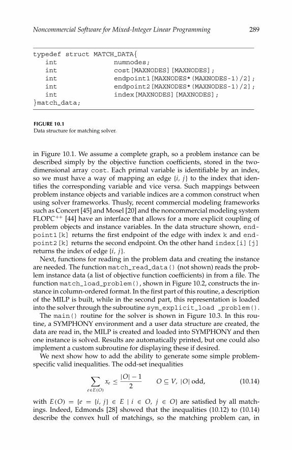
P1: ShashiAugust 12, 2005 11:38 1914 1914˙C010


typedef struct MATCH_DATAint numnodes;int cost[MAXNODES][MAXNODES];int endpoint1[MAXNODES*(MAXNODES-1)/2];int endpoint2[MAXNODES*(MAXNODES-1)/2];int index[MAXNODES][MAXNODES];

match_data;

FIGURE 10.1Data structure for matching solver.

in Figure 10.1. We assume a complete graph, so a problem instance can bedescribed simply by the objective function coefficients, stored in the two-dimensional array cost. Each primal variable is identifiable by an index,so we must have a way of mapping an edge i, j to the index that iden-tifies the corresponding variable and vice versa. Such mappings betweenproblem instance objects and variable indices are a common construct whenusing solver frameworks. Thusly, recent commercial modeling frameworkssuch as Concert [45] and Mosel [20] and the noncommercial modeling systemFLOPC++ [44] have an interface that allows for a more explicit coupling ofproblem objects and instance variables. In the data structure shown, end-point1[k] returns the first endpoint of the edge with index k and end-point2[k] returns the second endpoint. On the other hand index[i][j]returns the index of edge i, j.

Next, functions for reading in the problem data and creating the instanceare needed. The function match_read_data() (not shown) reads the prob-lem instance data (a list of objective function coefficients) in from a file. Thefunction match_load_problem(), shown in Figure 10.2, constructs the in-stance in column-ordered format. In the first part of this routine, a descriptionof the MILP is built, while in the second part, this representation is loadedinto the solver through the subroutine sym_explicit_load _problem().

The main() routine for the solver is shown in Figure 10.3. In this rou-tine, a SYMPHONY environment and a user data structure are created, thedata are read in, the MILP is created and loaded into SYMPHONY and thenone instance is solved. Results are automatically printed, but one could alsoimplement a custom subroutine for displaying these if desired.

We next show how to add the ability to generate some simple problem-specific valid inequalities. The odd-set inequalities

∑e∈E(O)

xe ≤ |O| − 12

O ⊆ V, |O| odd, (10.14)

with E(O) = e = i, j ∈ E | i ∈ O, j ∈ O are satisfied by all match-ings. Indeed, Edmonds [28] showed that the inequalities (10.12) to (10.14)describe the convex hull of matchings, so the matching problem can, in

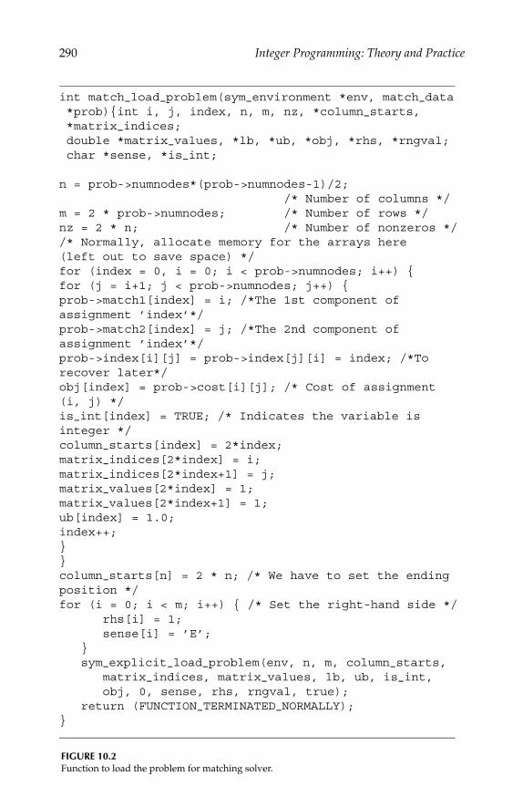
P1: ShashiAugust 12, 2005 11:38 1914 1914˙C010


int match_load_problem(sym_environment *env, match_data*prob)int i, j, index, n, m, nz, *column_starts,*matrix_indices;double *matrix_values, *lb, *ub, *obj, *rhs, *rngval;char *sense, *is_int;

n = prob->numnodes*(prob->numnodes-1)/2;/* Number of columns */

m = 2 * prob->numnodes; /* Number of rows */nz = 2 * n; /* Number of nonzeros *//* Normally, allocate memory for the arrays here(left out to save space) */for (index = 0, i = 0; i < prob->numnodes; i++) for (j = i+1; j < prob->numnodes; j++) prob->match1[index] = i; /*The 1st component ofassignment ’index’*/prob->match2[index] = j; /*The 2nd component ofassignment ’index’*/prob->index[i][j] = prob->index[j][i] = index; /*Torecover later*/obj[index] = prob->cost[i][j]; /* Cost of assignment(i, j) */is_int[index] = TRUE; /* Indicates the variable isinteger */column_starts[index] = 2*index;matrix_indices[2*index] = i;matrix_indices[2*index+1] = j;matrix_values[2*index] = 1;matrix_values[2*index+1] = 1;ub[index] = 1.0;index++;column_starts[n] = 2 * n; /* We have to set the endingposition */for (i = 0; i < m; i++) /* Set the right-hand side */

rhs[i] = 1;sense[i] = ’E’;

sym_explicit_load_problem(env, n, m, column_starts,

matrix_indices, matrix_values, lb, ub, is_int,obj, 0, sense, rhs, rngval, true);

return (FUNCTION_TERMINATED_NORMALLY);

FIGURE 10.2Function to load the problem for matching solver.

P1: ShashiAugust 12, 2005 11:38 1914 1914˙C010


int main(int argc, char **argv)

int termcode;char * infile;

/* Create a SYMPHONY environment */sym_environment *env = sym_open_environment();

/* Create the data structure for storing theinstance.*/user_problem *prob =(user_problem *)calloc(1, sizeof (user_problem));

sym_set_user_data(env, (void *)prob);sym_parse_command_line(env, argc, argv);sym_get_str_param(env, "infile_name", &infile);match_read_data(prob, infile);match_load_problem(env, prob);sym_solve(env);sym_close_environment(env);return(0);

FIGURE 10.3Main function for the matching solver.

theory, be solved as a linear program, albeit with an exponential numberof constraints.

The textbook of Grotschel, Lovasz, and Schrijver [37] describes how to ef-ficiently separate the odd-set inequalities in full generality, but for simplicity,we implement separation only for odd-set inequalities for sets of cardinal-ity three. This is done by brute force enumeration of triples, as shown inFigure 10.4. The function user_find_cuts() is the SYMPHONY callbackfor generating valid inequalities. The user is provided with the current frac-tional solution in a sparse vector format and asked to generate violated validinequalities. The function cg_add_explicit_cut() is used to report anyinequalities found. Even this simple separation routine can significantly re-duce the number of nodes in the branch-and-cut tree.

10.5.2 Branch and Price

The Three-Index Assignment Problem. The Three-Index Assignment Prob-lem (3AP) is that of finding a minimum-weight clique cover of the completetri-partite graph Kn,n,n, where n is redefined here to indicate the size of the un-derlying graph. Let I, J, and K be three disjoint sets with |I | = |J | = |K | = n

P1: ShashiAugust 12, 2005 11:38 1914 1914˙C010


int user_find_cuts(void *user, int varnum, int iter_num,int level, int index, double objval,int *indices, double *values, doubleub, double etol, int *num_cuts, int*alloc_cuts, cut_data ***cuts)

user_problem *prob = (user_problem *) user;double cut_val[3], edge_val[200][200];/* Matrix of edge values */int i, j, k, cutind[3], cutnum = 0;

/* Allocate the edge_val matrix to zero (we couldalso just calloc it) */ memset((char *)edge_val,0, 200*200*ISIZE);

for (i = 0; i < varnum; i++) edge_val[prob->node1[indices[i]]][prob->node2[indices[i]]] = values[i];

for (i = 0; i < prob->nnodes; i++)

for (j = i+1; j < prob->nnodes; j++)for (k = j+1; k < prob->nnodes; k++)

if (edge_val[i][j]+edge_val[j][k]+edge_val[i][k] > 1.0 + etol) /* Found violated triangle cut *//* Form the cut as a sparse vector */cutind[0] = prob->index[i][j];cutind[1] = prob->index[j][k];cutind[2] = prob->index[i][k];cutval[0] = cutval[1] = cutval[2] = 1.0;cg_add_explicit_cut(3, cutind,cutval, 1.0, 0, ’L’,

TRUE, num_cuts, alloc_cuts, cuts);cutnum++;

return(USER_SUCCESS);

FIGURE 10.4Cut generator for matching solver.

P1: ShashiAugust 12, 2005 11:38 1914 1914˙C010


and set H = I × J × K . Then, 3AP can be formulated as follows:

min∑

(i, j,k)∈H

cijkxijk,

∑( j,k)∈J ×K

xijk = 1 ∀i ∈ I, (10.15)

∑(i,k)∈I×K

xijk = 1 ∀ j ∈ J ,

∑(i, j)∈I×J

xijk = 1 ∀k ∈ K, (10.16)

xijk ∈ 0, 1 ∀(i, j, k), ∈ H.

In [10], Balas and Saltzman consider the use of the classical AssignmentProblem (AP) as a relaxation of 3AP in the context of Lagrangian relaxation.We use the same relaxation to reformulate the 3AP using a Dantzig-Wolfedecomposition (see Section 10.2.1.4 for a discussion of this technique). TheAP is a relaxation of the 3AP obtained by relaxing constraint (10.15). Let Fbe the set of feasible solutions to the AP. The Dantzig Wolfe (DW) reformula-tion of 3AP is then:

min∑s∈F

csλs ,

∑s∈F

∑

( j,k)∈J ×K

sijkλs

= 1 ∀i ∈ I,

∑s∈F

λs = 1,

λs ∈ Z+∀s ∈ F ,

where cs = (i, j,k)∈Hcijksijk for each s ∈ F . Relaxing the integrality constraintsof this reformulation, we obtain a relaxation of 3AP suitable for use in anLP-based branch-and-bound algorithm. Because of the exponential numberof columns in this linear program, we use a standard column generationapproach to solve it.

Implementing the Solver. The main classes to be implemented are theBCP_xx_user classes mentioned earlier and a few problem-specific classes.We describe the problem-specific classes first:

• AAP: This class is a container for holding an instance of 3AP. Datamembers include the dimension of the problem n and the objectivefunction vector.

• AAP_user_data: This class is derived from BCP_user_data andis used to store problem-specific information in the individual nodesof the search tree. Because we branch on the original variables xijk

and not the master problem variables λs , we must keep track of

P1: ShashiAugust 12, 2005 11:38 1914 1914˙C010


which variables have been fixed to 0 or 1 at a particular node,so that we can enforce these conditions in our column generationsubproblem.

• AAP_var: Each variable in the Dantzig-Wolfe reformulation rep-resents an assignment between members of sets J and K . In eachinstance of the class, the corresponding assignment is stored usinga vector that contains the indices of the assignment along with itscost.

Because BCP is a parallel code, every data structure must be accompa-nied by a subroutine that can both pack it into and unpack it from a char-acter buffer for the purposes of communicating the contents to other par-allel processes. For most built-in types, default pack and unpack routinesare predefined. For user-defined data structures, however, they must be pro-vided. Typically, such routines consist simply of a collection of calls to eitherBCP_buffer::pack()or BCP_buffer::unpack(), as appropriate, pack-ing or unpacking each data member of the class in turn. The user callbackclasses that must be modified are as follows:

• AAP_tm: This class is derived from BCP_tm_user and containsthe callbacks associated with initialization and tree management.The main callbacks implemented are initialize_core() andcreate_ root(). These methods define the core relaxation andthe initial LP relaxation in the root node.

• AAP_lp: This class is derived from BCP_lp_user and contains thecallbacks associated with the solution of the LP relaxations in eachsearch tree node. The main methods implemented are:

generate_vars_in_lp(): the subroutine that generates newvariables,compute_lower_bound(): returns a true lower bound in each

iteration (the LP relaxation does not yield a true lower boundunless no variables with negative reduced cost exist),restore_feasibility(): a subroutine that tries to generate

columns that can be used to restore the feasibility of a relaxationthat is currently infeasible,vars_to_cols(): a subroutine that generates the columns cor-

responding to a set of variables, so that they can be added to thecurrent relaxation,select_branching_candidates(): a subroutine that selects

candidates for strong branching. We branch on the original vari-ables xijk. Candidates are selected by the usual “most fractional”rule using the helper function branch_close_to_half(). Asecond function, append_branching_vars(), is called to cre-ate the branching objects, and

P1: ShashiAugust 12, 2005 11:38 1914 1914˙C010


set_user_data_for_children(): Stores the appropriate dataregarding what original variables were branched on in each childnode.

In addition to defining these classes, a few important parameters must beset. We have glossed over some details here, but the source code and a morethorough description of this example are available for download [34].

10.6 Benchmarking

In this section, we present computational results that show the relative per-formance of the black-box solvers reviewed in Section 10.4. Each solver wasbuilt with gcc 3.3 using the default build parameters. The experiments wererun under Linux RedHat v7.3 on an Intel Pentium III with an 1133MHz clockspeed and 512 MB of memory. The maximum CPU time allowed for eachsolver and each instance was two hours. For each of the codes, the defaultparameter settings were used on the instances, except for lp_solve, in whichthe default branching and node selection rules were changed to ones basedon pseudocosts.2

There were 122 problem instances included in the test: the instances ofmiplib33[16], miplib2003 [57], and 45 instances collected by the authors fromvarious sources. The instances collected by the authors are available fromthe Computational Optimization Research at Lehigh (COR@L) Web site [50].Table 10.4 shows the number of rows m, number of variables n, number ofcontinuous variables n − p, number of binary variables |B|, and number ofgeneral integer variables p − |B| for each instance in the test suite that is notalready available through MIPLIB.

In order to succinctly present the results of this extensive computationalstudy, we use performance profiles, as introduced by Dolan and More [25].A performance profile is a relative measure of the effectiveness of a solver swhen compared to a group of solvers S on a set of problem instances P . Tocompletely specify a performance profile, we need the following definitions:

• γps is a quality measure of solver s when solving problem p

• rps = γps/(mins∈S γps)

• ρs(τ ) = ∣∣p ∈ P | rps ≤ τ ∣∣ /|P|

2 The lp_solve command line was: lp_solve -mps name.mps -bfp ./bfp_LUSOL -timeout 7200 -time -presolve -presolvel -piva -pivla -piv2 -ca -B5 -Bd-Bg -si -s5 -se -degen -S1 -v4.3 With the exception of the instances air03, blend2, egout, enigma, flugpl, gen, khb05250 lseumisc03 misc06, mod008, mod010, p0033, p0201, p0282, rgn, stein27, vpm1, which at least five ofthe six solvers were able to solve in less than 2 minutes.

P1: ShashiAugust 12, 2005 11:38 1914 1914˙C010


TABLE 10.4

Characteristics of (non MIPLIB) Problem InstancesName m n n − p |B| p −|B| Name m n n − p |B| p −|B|22433 198 429 198 231 0 23588 137 368 137 231 0aligninq 340 1831 1 1830 0 bc1 1913 1751 1499 252 0bienst1 576 505 477 28 0 bienst2 576 505 470 35 0dano3_3 3202 13873 13804 69 0 dano3_4 3202 13873 13781 92 0dano3_5 3202 13873 13758 115 0 fiball 3707 34219 1 33960 258mcsched 2107 1747 2 1731 14 mkc1 3411 5325 2238 3087 0neos10 46793 23489 0 23484 5 neos11 2706 1220 320 900 0neos12 8317 3983 847 3136 0 neos13 20852 1827 12 1815 0neos14 552 792 656 136 0 neos15 552 792 632 160 0neos16 1018 377 0 336 41 neos17 486 535 235 300 0neos18 11402 3312 0 3312 0 neos1 5020 2112 0 2112 0neos20 2446 1165 198 937 30 neos2 1103 2101 1061 1040 0neos3 1442 2747 1387 1360 0 neos4 38577 22884 5712 17172 0neos5 63 63 10 53 0 neos6 1036 8786 446 8340 0neos7 1994 1556 1102 434 20 neos8 46324 23228 0 23224 4neos9 31600 81408 79309 2099 0 npmv07 76342 220686 218806 1880 0nsa 1297 388 352 36 0 nug08 912 1632 0 1632 0pg5_34 225 2600 2500 100 0 pg 125 2700 2600 100 0qap10 1820 4150 0 4150 0 ramos3 2187 2187 0 2187 0ran14x18_1 284 504 252 252 0 roy 162 149 99 50 0sp97ic 2086 1662 0 718 944 sp98ar 4680 5478 0 2796 2682sp98ic 2311 2508 0 1139 1369 sp98ir 1531 1680 0 871 809Test3 50680 72215 39072 7174 25969

Hence, ρs(τ ) is the fraction of instances for which the performance of solvers was within a factor of τ of the best. A performance profile for solver s is thegraph of ρs(τ ). In general, the “higher” the graph of a solver, the better therelative performance.

Comparison of MILP solvers directly on the basis of performance is prob-lematic in a number of ways. By compiling these codes with the same compileron the same platform and running them under identical conditions, we haveeliminated some of the usual confounding variables, but some remain. An im-portant consideration is the feasibility, optimality, and integrality tolerancesused by the solver. Dolan, More, and Munson [24] performed a careful studyof the tolerances used in nonlinear programming software and concluded thattrends of the performance profile tend to remain the same when tolerancesare varied. The differences in solver tolerances for these tests were relativelyminor, but these minor differences could lead to large differences in runtimeperformance. Another potential difficulty is the verification of solvers’ claimswith respect to optimality and feasibility of solutions. The authors made littleattempt to verify a posteriori that the solutions claimed as optimal or feasiblewere indeed optimal or feasible. The conclusions drawn here about the rela-tive effectiveness of the MILP solvers must be considered with these caveatsin mind.

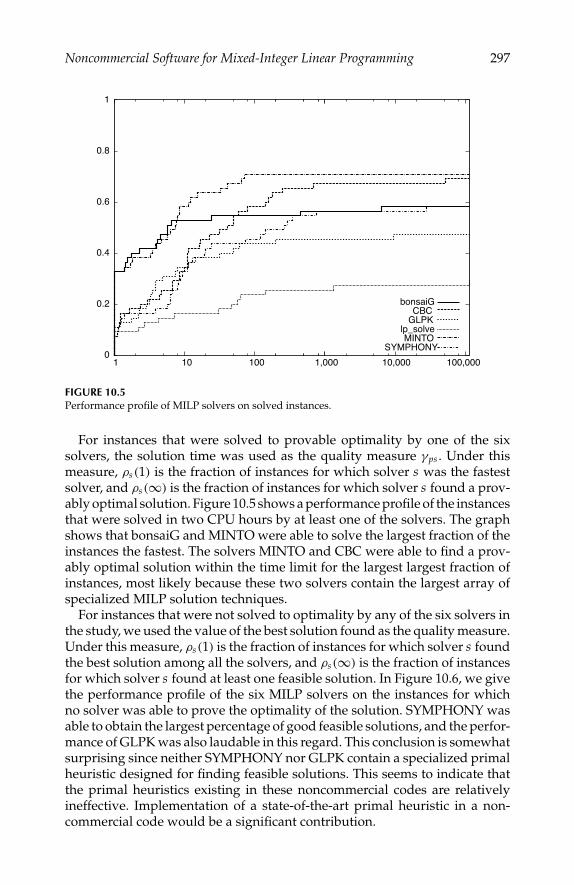
P1: ShashiAugust 12, 2005 11:38 1914 1914˙C010


SYMPHONYMINTO

lp_solveGLPKCBC

bonsaiG

100,000 10,000 1,000 100 101

1

0.8

0.6

0.4

0.2

0

FIGURE 10.5Performance profile of MILP solvers on solved instances.

For instances that were solved to provable optimality by one of the sixsolvers, the solution time was used as the quality measure γps . Under thismeasure, ρs(1) is the fraction of instances for which solver s was the fastestsolver, and ρs(∞) is the fraction of instances for which solver s found a prov-ably optimal solution. Figure 10.5 shows a performance profile of the instancesthat were solved in two CPU hours by at least one of the solvers. The graphshows that bonsaiG and MINTO were able to solve the largest fraction of theinstances the fastest. The solvers MINTO and CBC were able to find a prov-ably optimal solution within the time limit for the largest largest fraction ofinstances, most likely because these two solvers contain the largest array ofspecialized MILP solution techniques.

For instances that were not solved to optimality by any of the six solvers inthe study, we used the value of the best solution found as the quality measure.Under this measure, ρs(1) is the fraction of instances for which solver s foundthe best solution among all the solvers, and ρs(∞) is the fraction of instancesfor which solver s found at least one feasible solution. In Figure 10.6, we givethe performance profile of the six MILP solvers on the instances for whichno solver was able to prove the optimality of the solution. SYMPHONY wasable to obtain the largest percentage of good feasible solutions, and the perfor-mance of GLPK was also laudable in this regard. This conclusion is somewhatsurprising since neither SYMPHONY nor GLPK contain a specialized primalheuristic designed for finding feasible solutions. This seems to indicate thatthe primal heuristics existing in these noncommercial codes are relativelyineffective. Implementation of a state-of-the-art primal heuristic in a non-commercial code would be a significant contribution.

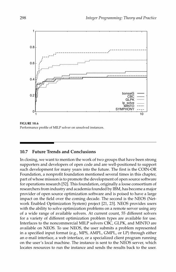
P1: ShashiAugust 12, 2005 11:38 1914 1914˙C010


SYMPHONYMINTO

lp_solveGLPK

CBCbonsaiG

101

1

0.8

0.6

0.4

0.2

0

FIGURE 10.6Performance profile of MILP solver on unsolved instances.

10.7 Future Trends and Conclusions

In closing, we want to mention the work of two groups that have been strongsupporters and developers of open code and are well-positioned to supportsuch development for many years into the future. The first is the COIN-ORFoundation, a nonprofit foundation mentioned several times in this chapter,part of whose mission is to promote the development of open source softwarefor operations research [52]. This foundation, originally a loose consortium ofresearchers from industry and academia founded by IBM, has become a majorprovider of open source optimization software and is poised to have a largeimpact on the field over the coming decade. The second is the NEOS (Net-work Enabled Optimization System) project [21, 23]. NEOS provides userswith the ability to solve optimization problems on a remote server using anyof a wide range of available solvers. At current count, 55 different solversfor a variety of different optimization problem types are available for use.Interfaces to the noncommercial MILP solvers CBC, GLPK, and MINTO areavailable on NEOS. To use NEOS, the user submits a problem representedin a specified input format (e.g., MPS, AMPL, GMPL, or LP) through eitheran e-mail interface, a web interface, or a specialized client program runningon the user’s local machine. The instance is sent to the NEOS server, whichlocates resources to run the instance and sends the results back to the user.

P1: ShashiAugust 12, 2005 11:38 1914 1914˙C010


Because the job runs remotely, this provides the user with the ability to testmultiple solvers without downloading and installing each of them individu-ally. The NEOS project has been solving optimization problems on-line since1991, and currently handles over 10,000 optimization instances each month.

As for the future, we see no slowing of the current trend toward the devel-opment of competitive noncommercial software for solving MILPs. A num-ber of exciting new open source projects are currently under developmentand poised to further expand the offerings to users of optimization soft-ware. Among these is the Abstract Library for Parallel Search (ALPS), a C++class library for implementing parallel search algorithms planned that is theplanned successor to BCP [86]. ALPS will further generalize many of the con-cepts present in BCP, providing the ability to implement branch-and-boundalgorithms for which the bounding procedure is not necessarily LP-based.A second framework, called DECOMP, will provide the ability to automatethe solution of decomposition-based bounding problems, i.e., those based onLagrangian relaxation or Dantzig-Wolfe decomposition. Both of these frame-works will be available as part of the COIN-OR software suite. A new gen-eration of the Open Solver Interface supporting a much wider range of prob-lem types and with better model-building features is under development byCOIN-OR, along with a new open standard based on LPFML for describingmathematical programming instances [32]. Finally, a MILP solver that inte-grates techniques from constraint programming with those described here isalso under development and due out soon [1].

On the whole, we were impressed by the vast array of packages and auxil-iary tools available, as well as the wide variety of features exhibited by thesecodes. The most significant features still missing in open codes are effectivelogical preprocessors and primal heuristics. More effort is needed in develop-ing tools to fill this gap. Although noncommercial codes will most likely con-tinue to lag behind commercial codes in terms of raw speed in solving genericMILPs out of the box, they generally exhibit a much greater degree of flexibil-ity and extensibility. This is especially true of the solver frameworks, whichare designed specifically to allow the development of customized solvers. Anumber of features that appear in noncommercial codes, such as parallelism,the ability to support column generation, and the ability to solve multi-criteriaMILPs, simply do not exist in most commercial codes. Although the noncom-mercial codes are in general slower than the best commercial codes, we believethat many users will be genuinely satisfied with the features and performanceof the codes reviewed here and we look forward to future developments inthis fast-growing area of software development.

Acknowledgment

The authors would like to thank Kjell Eikland, John Forrest, Matthew Galati,Lou Hafer, and Matthew Saltzman for their insightful comments that helpedto improve the chapter.

P1: ShashiAugust 12, 2005 11:38 1914 1914˙C010


References

1. Achterberg, T., SCIP — a framework to integrate constraint and mixed integerprogramming, Technical Report ZIB-Report 04-19, Konrad-Zuse-Zentrum furInformationstechnik Berlin, Takustr. 7, Berlin, 2005.

2. Achterberg, T., Koch, T., and Martin, A., Branching rules revisited, OperationsResearch Letters, 33, 42, 2004.

3. Applegate, D., Bixby, R., Cook, W., and Chvatal, V., 1996, Personal communica-tion.

4. Atamturk, A., Nemhauser, G., and Savelsbergh, M. W. P., Conflict graphs in inte-ger programming, Technical Report LEC-98-03, Georgia Institute of Technology,1998.

5. Atamturk, A., Nemhauser, G., and Savelsbergh, M. W. P., Conflict graphs insolving integer programming problems, European J. Operational Research, 121,40, 2000.

6. Atamturk, A. and Savelsbergh, M., Integer-programming software systems,Annals of Operations Research, 2005, To appear, Available from http://www.isye.gatech.edu/faculty/Martin_Savelsbergh/publications/ipsoftware-final.pdf.

7. Balas, E., Facets of the knapsack polytope, Mathematical Programming, 8, 146,1975.

8. Balas, E., Ceria, S., Cornuejols, G., and Natraj, N., Gomory cuts revisited, Op-erations Research Letters, 19, 1, 1999.

9. Balas, E. and Martin, R., Pivot and complement: a heuristic for 0-1 programming,Management Science, 26, 86, 1980.

10. Balas, E. and Saltzman, M., An algorithm for the three-index assignment prob-lem, Operations Research, 39, 150, 1991.

11. Balas, E., Schmieta, S., and Wallace, C., Pivot and shift — A mixed integerprogramming heuristic, Discrete Optimization, 1, 3, 2004.

12. Beale, E. M. L., Branch and bound methods for mathematical programmingsystems, in Discrete Optimization II, edited by Hammer, P. L., Johnson, E. L., andKorte, B. H., pages 201–219, North Holland Publishing Co., 1979.

13. Beale, E. W. L. and Tomlin, J. A., Special facilities in a general mathematicalprogramming system for nonconvex problems using ordered sets of variables,in Proceedings of the 5th International Conference on Operations Research, edited byLawrence, J., pages 447–454, 1969.

14. Benichou, M. et al., Experiments in mixed-integer linear programming, Math-ematical Programming, 1, 76, 1971.

15. Berkelaar, M., lp_solve 5.1, 2004, Available from http://groups.yahoo.com/group/lp_solve/.

16. Bixby, R. E., Ceria, S., McZeal, C. M., and Savelsbergh, M. W. P., An updatedmixed integer programming library: MIPLIB 3.0, Optima, 58, 12, 1998.

17. Borndorfer, R. and Weismantel, R., Set packing relaxations of some integer pro-grams, Mathematical Programming, 88, 425, 2000.

18. Chvatal, V., Linear Programming, W. H. Freeman and Co., New York, 1983.19. COIN-OR: Computational Infrastructure for Operations Research, 2004,

http://www.coin-or.org.20. Colombani, Y. and Heipcke, S., Mosel: An extensible environment for modeling

and programming solutions, in Proceedings of the Fourth International Workshop

P1: ShashiAugust 12, 2005 11:38 1914 1914˙C010


on Integration of AI and OR Techniques in Constraint Programming for CombinatorialOptimisation Problems (CP-AI-OR’02), edited by Jussien, N. and Laburthe, F.,pages 277–290, 2002.

21. Czyzyk, J., Mesnier, M., and More, J., The NEOS server, IEEE Journal on Com-putational Science and Engineering, 5, 68, 1998.

22. Danna, E., Rothberg, E., and LePape, C., Exploring relaxation induced neigh-borhoods to improve MIP solutions, Mathematical Programming, 2004, To appear.

23. Dolan, E., Fourer, R., More, J., and Munson, T., Optimization on the NEOS server,SIAM News, 35, 8, 2002.

24. Dolan, E., More, J., and Munson, T., Optimality measures for performance pro-files, Preprint ANL/MCS-P1155-0504, Mathematics and Computer Science Di-vision, Argonne National Lab, 2004.

25. Dolan, E. and More, J., Benchmarking optimization software with performanceprofiles, Mathematical Programming, 91, 201, 2002.

26. Driebeek, N. J., An algorithm for the solution of mixed integer programmingproblems, Management Science, 12, 576, 1966.

27. Eckstein, J., Parallel branch-and-bound methods for mixed integer program-ming, SIAM News, 27, 12, 1994.

28. Edmonds, J., Maximum matching and a polyhedron with 0-1 vertices, Journalof Research of the National Bureau of Standards, 69B, 125, 1965.

29. Fischetti, M. and Lodi, A., Local branching, Mathematical Programming, 98, 23,2002.

30. Forrest, J., CBC, 2004, Available from http://www.coin-or.org/.31. Forrest, J. J. H., Hirst, J. P. H., and Tomlin, J. A., Practical solution of large scale

mixed integer programming problems with UMPIRE, Management Science, 20,736, 1974.

32. Fourer, R., Lopes, L., and Martin, K., LPFML: A W3C XML schema for linearprogramming, 2004, Available from http://www.optimization-online.org/DB_HTML/2004/02/817.html.

33. Fourer, R., Gay, D. M., and Kernighan, B. W., AMPL: A Modeling Language forMathematical Programming, The Scientific Press, 1993.

34. Galati, M., COIN-OR tutorials, 2004, Available from http://coral.ie.lehigh.edu/∼coin/.

35. Gauthier, J. M. and Ribiere, G., Experiments in mixed-integer linear program-ming using pseudocosts, Mathematical Programming, 12, 26, 1977.

36. Gomory, R. E., An algorithm for the mixed integer problem, Technical ReportRM-2597, The RAND Corporation, 1960.

37. Grotschel, M., Lovasz, L., and Schrijver, A., Geometric Algorithms and Combina-torial Optimization, Springer-Verlag, New York, 1988.

38. Gu, Z., Nemhauser, G. L., and Savelsbergh, M. W. P., Cover inequalities for0-1 linear programs: Computation, INFORMS Journal on Computing, 10, 427,1998.

39. Gu, Z., Nemhauser, G. L., and Savelsbergh, M. W. P., Lifted flow covers formixed 0-1 integer programs, Mathematical Programming, 85, 439, 1999.

40. Gu, Z., Nemhauser, G. L., and Savelsbergh, M. W. P., Sequence independentlifting, Journal of Combinatorial Optimization, 4, 109, 2000.

41. Hafer, L., bonsaiG 2.8, 2004, Available fromhttp://www.cs.sfu.ca/∼lou/BonsaiG/dwnldreq.html.

42. Hammer, P. L., Johnson, E. L., and Peled, U. N., Facets of regular 0-1 polytopes,Mathematical Programming, 8, 179, 1975.

P1: ShashiAugust 12, 2005 11:38 1914 1914˙C010


43. Hoffman, K. and Padberg, M., Solving airline crew-scheduling problems bybranch-and-cut, Management Science, 39, 667, 1993.

44. Hultberg, T., FlopC++, 2004, Available from http://www.mat.ua.pt/thh/flopc/.

45. ILOG concert technology, http://www.ilog.com/products/optimiza-tion/tech/concert.cfm.

46. Junger, M. and Thienel, S., The ABACUS system for branch and cut and pricealgorithms in integer programming and combinatorial optimization, SoftwarePractice and Experience, 30, 1325, 2001.

47. Ladanyi, L., Parallel Branch and Cut and Its Application to the Traveling SalesmanProblem, PhD thesis, Cornell University, 1996.

48. Ladanyi, L., BCP, 2004, Available from http://www.coin-or.org/.49. Linderoth, J. T. and Savelsbergh, M. W. P., A computational study of search

strategies in mixed integer programming, INFORMS Journal on Computing,11, 173, 1999.

50. Linderoth, J., MIP instances, 2004, Available fromhttp://coral.ie.lehigh.edu/mip-instances.

51. Lougee-Heimer, R., The Common Optimization INterface for Operations Re-search, IBM Journal of Research and Development, 47, 57, 2003.

52. Lougee-Heimer, R., Saltzman, M., and Ralphs, T., ‘COIN’ of the OR Realm,OR/MS Today, October, 2004.

53. Makhorin, A., GLPK 4.2, 2004, Available fromhttp://www.gnu.org/ soft-ware/glpk/glpk.html.

54. Marchand, H., A Study of the Mixed Knapsack Set and Its Use to Solve Mixed IntegerPrograms, PhD thesis, Facult’e des SciencesAppliquees, Universite Catholiquede Louvain, 1998.

55. Marchand, H. and Wolsey, L., Aggregation and mixed integer rounding to solveMIPs, Operations Research, 49, 363, 2001.

56. Margot, F., BAC: A BCP based branch-and-cut example, Report RC22799, IBMResearch, 2004.

57. Martin, A., Achterberg, T., and Koch, T., MIPLIB 2003, Avaiable from http://miplib.zib.de.

58. Mitra, G., Investigation of some branch and bound strategies for the solution ofmixed integer linear programs, Mathematical Programming, 4, 155, 1973.

59. Nediak, M. and Eckstein, J., Pivot, cut, and dive: A heuristic for mixed 0-1integer programming, Technical Report RUTCOR Research Report RRR 53-2001,Rutgers University, 2001.

60. Nemhauser, G. and Savelsbergh, M., MINTO 3.1, 2004, Available fromhttp://coral.ie.lehigh.edu/minto/.

61. Nemhauser, G. and Wolsey, L., A recursive procedure for generating all cuts for0-1 mixed integer programs, Mathematical Programming, 46, 379, 1990.

62. Nemhauser, G. and Wolsey, L. A., Integer and Combinatorial Optimization, JohnWiley and Sons, New York, 1988.

63. Nemhauser, G. L. and Sigismondi, G., A strong cutting plane/branch-and-bound algorithm for node packing, Journal of the Operational Research Society,43, 443, 1992.

64. Nemhauser, G. L. and Trotter Jr., L. E., Properties of vertex packing and inde-pendence system polyhedra, Mathematical Programming, 6, 48, 1974.

65. Padberg, M., On the facial structure of set packing polyhedra, MathematicalProgramming, 5, 199, 1973.

P1: ShashiAugust 12, 2005 11:38 1914 1914˙C010


66. Padberg, M., Linear Optimization and Extensions, Springer-Verlag, New York,1995.

67. Ralphs, T. K., Ladanyi, L., and Saltzman, M. J., Parallel branch, cut, and pricefor large-scale discrete optimization, Mathematical Programming, 98, 253, 2003.

68. Ralphs, T., Parallel Branch and Cut for Vehicle Routing, PhD thesis, Cornell Uni-versity, 1995.

69. Ralphs, T., SYMPHONY 5.0, 2004, Available from http://www.branchand-cut.org/SYMPHONY/.

70. Ralphs, T., SYMPHONY Version 5.0 User’s Manual, Technical Report 04T-020,Lehigh University Industrial and Systems Engineering, 2004, Available fromhttp://www.lehigh.edu/∼tkr2/research/pubs.html.

71. Ralphs, T. and Guzelsoy, M., The SYMPHONY callable library for mixedinteger programming, in The Proceedings of the Ninth Conference of the IN-FORMS Computing Society, 2005, To appear, Available from http://www.lehigh.edu/∼tkr2/research/pubs.html.

72. Ralphs, T., Saltzman, M., and Wiecek, M., An improved algorithm for biob-jective integer programming, Annals of Operations Research, 2005, To appear,Available fromhttp://www.lehigh.edu/∼tkr2/research/pubs.html.

73. Roy, J.-S., PuLP : A linear programming modeler in Python, Available fromhttp://www.jeannot.org/∼js/code/index.en.html#PuLP.

74. Savelsbergh, M. W. P., Preprocessing and probing techniques for mixed integerprogramming problems, ORSA Journal on Computing, 6, 445, 1994.

75. Schrage, L. and Wolsey, L. A., Sensitivity analysis for branch and bound linearprogramming, Operations Research, 33, 1008, 1985.

76. Schrijver, A., Theory of Linear and Integer Programming, Wiley, Chichester, 1986.77. Sidebottom, G., Satisfaction of constraints on nonnegative integer arithmetic

expressions, Open File Report 1990-15, Alberta Research Council, 6815 8th Street,Calgary, Alberta, CA T2E 7H7, 1990.

78. Thienel, S., ABACUS 2.3, 2004, Available from http://www.informatik.uni-koeln.de/abacus/.

79. Tomlin, J. A., An improved branch-and-bound method for integer program-ming, Operations Research, 19, 1070, 1971.

80. Trick, M. and Guzelsoy, M., Simple walkthrough of building a solverwith symphony, 2004, Available from ftp://branchandcut.org/pub/reference/SYMPHONY-Walkthrough.pdf.

81. van Heesch, D., Doxygen documentation system, 2004, Available fromhttp://www.doxygen.org/.

82. Vanderbeck, F., A generic view of Dantzig-Wolfe decomposition in mixedinteger programming, Working paper, 2003, Available from http://www.math.u-bordeaux.fr/∼fv/papers/dwcPap.pdf.

83. Wolsey, L. A., Faces for a linear inequality in 0-1 variables, Mathematical Pro-gramming, 8, 165, 1975.

84. Wolsey, L. A., Valid inequalities for mixed integer programs with generalizedand variable upper bound constraints, Discrete Applied Mathematics, 25, 251, 1990.

85. Wolsey, L. A., Integer Programming, John Wiley and Sons, New York, 1998.86. Xu, Y., Ralphs, T., Ladanyi, L., and Saltzman, M., ALPS: A framework for

implementing parallel search algorithms, in The Proceedings of the Ninth Con-ference of the INFORMS Computing Society, 2005, To appear, Available fromhttp://www.lehigh.edu/∼tkr2/research/pubs.html.

87. ZIMPL, Available from http://www.zib.de/koch/zimpl/.

P1: ShashiAugust 12, 2005 11:38 1914 1914˙C010

P1: Naresh

August 23, 2005 10:52 1914 1914˙Index

Index

A

ABACUS, 255, 273–275, 277Abstract Library for Parallel Search

(ALPS), 298Adaptive clause weights (ACW),

Boolean optimizationproblems

computational results, 9–10performance profiles, 15–16search improvements, local, 5

Adaptive move evaluation scheme, 4Adaptive search, greedy randomized,

see GRASPAffinity effect, cross-problem, 227Aggregate formulation, vessel

scheduling modelsmultiple sources and destinations,

178–182single source and destination,

150–153Airlines, scheduling models and

airport closures, 111–134basic model, 114–118case study, 126–132solution methods, 124–126strategic models, 119–124

ferrying idle aircraft, 123–124flight delays, 120–121multi-stop flight modification,

122–123swap of aircraft types, 119, 120

Algorithm control, MILP softwareprograms, see specific programs

Algorithmic considerations, retailassortment planning, 238

ALPS (Abstract Library for ParallelSearch), 298

AMPL, 271–273, 298Application Programming Interface

(API), 272, 274

Assignment problemgeneralized, 39–54

branch-and-bound algorithm,48–50

computational results, 50–53methods for decreasing upper

bound for (P), 47–48methods for increasing lower

bound for (P), 42–47model formulation, 40previous work, 40–42

three-index, 103–105Assortment, retail, see also Retail

assortment planningcompeting, evaluation of, 229constraints on, 231–232number effect, 246, 247

B

Backward-looking methods, 58–59,267

BCP, 255, 273–274, 277–279Best estimate method, 269Best-estimate search, 275Best-first search, 269, 275Best move, probabilistic move

acceptance, 5Best projection method, 269, 275Binary variables, MILP, 255Black-box solvers, 274

benchmarking, 294–298user interfaces, 270–272

Blossom inequalities, 83b-Matching relaxation, 100BonsaiG, 255, 274, 279–280Boolean optimization problems

(BOOP), 2–17computational results, 9–15

adaptive clause weights, effectsof, 9–10

305

P1: Naresh

August 23, 2005 10:52 1914 1914˙Index

306 Index

comparison with GRASP, 12–13performance profiles, 15–16persistent attractiveness measure

and marginal conditionalvalidity, 10–12

probabilistic move acceptance,effects of, 10

results for weighted maximumsatisfiability, 13–15

constructive methods, 6–8comparison with GRASP, 8marginal conditional validity

(MCV), 7–8persistent attractiveness measure

(PAM), 6–7local search improvements, 4–6

adaptive clause weights, 5probabilistic move acceptance,

5–6move evaluation function, 4problem formulation, 2–3search basics, 3–4weighted maximum satisfiability,

8–9Bounded duality, 21Bounding phase, branch-and-bound

algorithm, 256Bounding procedures, ILP, 57–58

airline flights, 125–126decomposition principles,

60–61generalized assignment problem

branch-and-bound algorithm,48–50

methods for decreasing upperbound for (P), 47–48

methods for increasing lowerbound for (P), 42–47

reducing gap, 41Branch-and-bound algorithm

softwarebranching, 266–269lower bounds

column generation, 264–265logical preprocessing, 258reduced cost tightening, 264valid inequalities, 258–264

search strategy, 269–270upper bounding methods,

265–266

Branch-and-bound methods, 20airline flights, 125generalized assignment problem,

48–50, 54solver frameworks, 273

Branch and cut method, 259, 273Branch and price algorithm

case studies, 291–294solver frameworks, 273

Branchingbranch-and-bound algorithm, 257software, 266–269, 275; see also

specific programsBranching on hyperplane, 268Breadth-first search, 275Buyer’s problem, retail assortment

planning, 234–235decomposition, 233formulation, 234–236

C

C++ programming language, 271–274Callable API, 272, 274Callable libraries, user interfaces,

272–273Callback classes, BCP, 277Cancellation model, airline, 113Candidate problem

branch-and-bound algorithm, 49branch-and-bound algorithm

subproblem, 256–257generalized assignment problem,

44, 46, 54Carry/no carry rules, retail

assortment planning, 237CBC, 255, 274

benchmarking, 296, 297features of, 280–282interfaces, 298

CGL (Cut Generation Library), 260Children, MILP, 256Clique inequalities, 262Coefficient lifting, 43Coefficient reduction,

branch-and-bound algorithm,258

COIN-OR (ComputationalInfrastructure for OperationsResearch), 260, 279, 299

P1: Naresh

August 23, 2005 10:52 1914 1914˙Index

Index 307

Column generationdecompose and cut subproblem, 95lower bounds, branch-and-bound

algorithm methods, 264–265master problem solution, 96retail assortment planning, see

Retail assortment planningComb inequalities

price and cut, 81–83, 88template paradigm, 93

Commercial software, 255Commutation, data cycle map

frames, 198, 201, 202Complete enumeration,


COMPSys, 277Computational Infrastructure for

Operations Research(COIN-OR), 260, 279, 299

Computational resultsBoolean optimization problems,

9–15adaptive clause weights, effects

of, 9–10comparison with GRASP, 12–13performance profiles, 15–16persistent attractiveness measure

and marginal conditionalvalidity, 10–12

probabilistic move acceptance,effects of, 10

results for weighted maximumsatisfiability, 13–15

generalized assignment problem,50–53

retail assortment planning, 239–248separable nonlinear integer

programming, 33–35vessel scheduling, single source

and destination, 153–154Conditional feasibility tests,

generalized assignmentproblem, 47

Conflict graph, 262Conjunctive normal form (CNF), 3Constraint analysis,


Constraint matrix, 59, 255

Constraint programming, 299Constructive methods, Boolean

optimization problems, 6–8comparison with GRASP, 8marginal conditional validity

(MCV), 7–8persistent attractiveness measure

(PAM), 6–7Continuous approximation, bound

algorithm, 58Continuous variables, MILP, 255Convergent Lagrangian methods

airline flights, 125separable nonlinear integer

programming, 25–33domain cut method, 29–33objective level cut, 25–29

Convex envelope function, 22, 25Convex hull, 25, 26Core relaxation, BCP, 277Corner point, perturbation function,

22Cost-based heuristic procedure, ship

scheduling, 142Cost tightening, lower bounds,

branch-and-bound algorithmmethods, 264

Cover inequalities, 260–262, 274CPLEX, 2, 16, 54, 255, 274, 284,

285ship scheduling, 153–157solver software, 52

Cross product affinity effect, 227Cut and branch method,


Cut Generation Library (CGL), 260Cutting/cutting plane method

airline flights, 125decomposition integrated solutions

price and cut, 79–90relax and cut, 90–92

decomposition principles, 61,64–68

decomposition subproblemsolution, 92–96

decompose and cut, 94–96separating solutions with known

structure, 93–94template paradigm, 93

P1: Naresh

August 23, 2005 10:52 1914 1914˙Index

308 Index

separable nonlinear integerprogramming, 25–33

domain cut method, 29–33objective level cut, 25–29

separation procedures, 59, 93software, 98

D

Dantzig-Wolfe method, 61, 77, 78, 87automated solutions, 299decomposition principles, 68–76price and cut, 80, 81software, 97

Data cycle map optimization, 195–216equivalency proof, 218–219generalized set packaging model,

207–209LCM proof, 217–218minor frame design, 199–207optimization models, 207–209strengthening set packing integer

programming model, 209–215multi-word parameters, 212–215pairwise slot constraints, 210–212

structure of data cycle maps, 196,197–198

DECOMP, 97, 298–299Decompose and cut decomposition

subproblem, 92, 94–96Decomposition, 57–107

airline flights, 132applications, 98–107

Steiner tree problem, 105–107three-index assignment problem,

103–105vehicle routing problem, 99–103

automated solutions, 299conclusions and future work, 107cutting subproblem solution, 92–96

decompose and cut, 94–96separating solutions with known

structure, 93–94template paradigm, 93

definitions and notation, 59–60integrated methods, 78–92

price and cut, 79–90relax and cut, 90–92

master problem solution, 96–97nonlinear Lagrangian theory and,

24–25

principle of, 60–78cutting plane method, 64–68Dantzig-Wolfe method, 68–76effect of applying, 61–64Lagrangian method, 76–78

retail assortment planning, 233–234ship scheduling, 140software, 97–98terminology, 57–59

Definitions and notation,decomposition, 59–60

Degree-constrained k-tree (k-DCT),100, 101, 102

Degree constraints, TravelingSalesman Problem, 63–64

Demand structure, vessel schedulingmodel, 170

Depth-first search, 269–270, 275DesigningDisjunctive normal form (DNF), 3Diversification of search, 3Domain cut methods

numerical results, 34, 35separable nonlinear integer

programming, 29–33Duality, separable nonlinear integer

programming, 20–25Duality bound, 21, 25, 26Duality gap, 20, 21, 25

domain cut method, 29, 31objective level cut, 26, 28

Dual multipliers, Lagrangianmethod, 77

Dual searchobjective level cut, 26separable nonlinear integer

programming, 36Dual solution

master problem solution, 96price and cut, 90

DYLP, 279Dynamic programming, 20, 27, 28

E

Effective algorithm, decompositionprinciples, 61

Efficient frame size, data cycle mapframes, 199

Enumeration, branch-and-boundalgorithm, 49

P1: Naresh

August 23, 2005 10:52 1914 1914˙Index

Index 309

Envelope function, convex, 22, 25Equivalency proof, data cycle map

optimization, 218–219Estimate-based search strategies, 269Evaluation, move, 3Exact integer solution method,

network flow problems,124–125

Expected revenue/profit functions(ER/PF), retail assortmentplanning, 230–231, 235

Exponential service timedistributions, ship scheduling,142

Extensible markup language (XML),271

F

Facet-defining inequalitiesbranch-and-bound algorithm, 259cutting plane method, 64–68, 87

Facet identification problem, 259FATHOM, 48, 49Feasibility tests

branch-and-bound algorithm, 49generalized assignment problem,

47, 48Feasible solution generator,


Feasible solutions, generalizedassignment problem, 54

File formats, 270–271, 274Fleet deployment

airline flights, see Airlines,scheduling models and airportclosures

ocean vessels, see Vessel schedulingFlight arc, 115–117Flight scheduling, see Airlines,

scheduling models and airportclosures

Flight swaps, 119, 120FLOPC++, 273, 288Flow cover inequalities, 261–262,

274Flow decomposition method, airline

flights, 132Formats, raw file, 270–271Forward-looking methods, 267

Fractional solution,branch-and-bound algorithm,256

Frames, data cycle maps, 196,197–198; see also Data cyclemap optimization

Framework API, 274Frameworks, solver, user interfaces,

273Free Software Foundation (FSF), 282

G

GAMS, 273Generalized assignment problem,

39–54branch-and-bound algorithm, 48–50computational results, 50–53methods for decreasing upper

bound for (P), 47–48methods for increasing lower

bound for (P), 42–47model formulation, 40previous work, 40–42

Generalized upper bound (GUB)branching, 268

Generalized upper bound (GUB)cover inequalities, 260–261, 274

GLPK, 272, 274benchmarking, 297, 298features of, 282–283interfaces, 298

GMPL, 272, 282, 298GNU, 279GNU MathProg (GMPL), 271–272,

282, 298Gomory inequalities, 263, 274GRASP, 2

Boolean optimization problemscomputational results, 12–13constructive methods, 8

Greedy heuristic, airline flights, 113Greedy Randomized Adaptive Search

Procedure, see GRASPGround arc, 116GSEC, violated, 100–102GUB (generalized upper bound)

branching, 268GUB (generalized upper bound)

cover inequalities, 260–261, 274

P1: Naresh

August 23, 2005 10:52 1914 1914˙Index

310 Index

H

Heuristic rules, price and cut, 90Hull, convex, 25Hybrid search methods, 269, 270, 275Hyperplane, branching on, 268

I

ILOG Concert Technology, 272Implication inequalities, 262, 274Improving, valid inequalities, 259Incumbent, branch-and-bound

algorithm, 256Inequalities

combprice and cut, 81–83template paradigm, 93

validimproving, 259relax and cut, 90separation procedures, 60software packages, 274–275template paradigm, 93

valid, branch and bound algorithm,258–264

black-box solvers, 274clique inequalities, 262flow cover inequalities, 261–262generalized upper bound (GUB)

cover inequalities, 260–261Gomory inequalities, 263implication inequalities, 262knapsack cover inequalities,

260mixed-integer rounding

inequalities, 263–264violated, price and cut, 85, 89

Inner approximation methods,polyhedron approximation,58–59

Inner representation, polyhedronapproximation, 58

Integer variables, MILP, 255Integer vectors, polyhedron, 59Integrality requirement, ILP, ’, 61Integrated methods, decomposition,

78–92price and cut, 79–90relax and cut, 90–92

Interior point methods, 97

Inventory holding cost effect, retailassortment planning, 245–246

Inventory planning, see Retailassortment planning

IRIG regulations/standards, 196, 198,199, 201, 202

K

k-DCT (degree-constrained k-tree),100, 101, 102

Knapsack constraints, generalizedassignment problem, 42–43

Knapsack inequalities, 274Knapsack problem, see also Separable

nonlinear integerprogramming

generalized assignment problem,44, 45, 46, 47–48

knapsack cover inequalities, 260retail assortment planning, 227

L

Lagrangian duality, 21Lagrangian method, 97

decomposition principles, 61, 76–78retail assortment planning, 226

Lagrangian relaxation methodsairline flights, 125, 128automated solutions, 299branch-and-bound algorithm, 48,

49generalized assignment problem,

41, 43–46, 53objective level cut, 26–27separable nonlinear integer

programming, 20–25ship scheduling, 140

Languages, modeling, 271–272LCM proof, data cycle map

optimization, 217–218Libraries, callable, 274

Cut Generation Library (CGL), 260user interfaces, 272–273

LIFO rule, 49, 53Lifted simple generalized flow cover

inequality, 262LINDO, 255, 284Linear optimization model, retail

assortment planning, 228

P1: Naresh

August 23, 2005 10:52 1914 1914˙Index

Index 311

Linear programming (LP) relaxation,255

bounding methods, 61branch-and-bound algorithm, 256generalized assignment problem, 53

Linear programming (LP) solver, 298data cycle map optimization, 208software, 274

Linear relaxation model, shipscheduling, 154

Local searchBoolean optimization problems,

3–6adaptive clause weights, 5probabilistic move acceptance,

5–6retail assortment planning, 227

Logical preprocessing,branch-and-bound algorithmmethods, 258

Lower boundsairline flights, 125branch-and-bound algorithm

methods, 257, 258–265column generation, 264–265logical preprocessing, 258reduced cost tightening, 264valid inequalities, 258–264

generalized assignment problem,methods for increasing, 42–47

software, see specific programslp_solve, 255, 274

benchmarking, 297features of, 283–284

LPFML, 271, 299LP relaxation, see Linear

programming (LP) relaxation

M

Major frame, data cycle map, 196example problem, 203–204structure of maps, 197, 198

Marginal conditional validity (MCV),Boolean optimizationproblems, 16

computational results, 10–12constructive methods, 7–8

Master problem, decompositiondefined, 58

integrated methods, 59solution of, 96–97

Matching problem,branch and cut, 288Mathematical Programming System

(MPS) format, 271, 298Maximum satisfiability, weighted, 2,

8–9, 13–15, 16Maxtrix coefficients,


Memory allocation, Lagrangianrelaxation methods, 125

Metaheurustics, strong local searchcombined with, 227

MILP (mixed-integer linearprograms), see Software

Minimum 1-Tree Problem, 64, 72Minimum 2-Matching Problem, 84Minimum Degree-Constrained k-Tree

Problem, 100Minimum Spanning Tree Problem,

105–106Minor frame, data cycle map, 196

designing, 199–207example problem, 203–204structure of maps, 197–198

MINTO, 255, 274benchmarking, 296, 297features of, 284–286interfaces, 298

Mixed-integer programssoftware, see Softwarevessel scheduling models, see also

Vessel schedulingmultiple sources and

destinations, 174–177single source and destination,

140, 141, 142Mixed-integer rounding inequalities,

263–264, 274Model formulation, generalized

assignment problem, 40Modeling languages, 271–272Modeling objects, BCP, 277–278Move, search basics, 3Move acceptance, probabilistic, 5–6,

10, 15–16Move evaluation

adaptive, 4search basics, 3

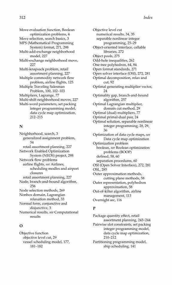
P1: Naresh

August 23, 2005 10:52 1914 1914˙Index

312 Index

Move evaluation function, Booleanoptimization problems, 4

Move selection, search basics, 3MPS (Mathematical Programming

System) format, 271, 298Multi-add-exchange neighborhood

model, 227Multi-exchange neighborhood move,

227Multi-knapsack problem, retail

assortment planning, 227Multiple commodity network flow

problem, airline flights, 125Multiple Traveling Salesman

Problem, 100, 102–103Multipliers, Lagrange, 77Multi-shift neighborhood moves, 227Multi-word parameters, set packing

integer programming model,data cycle map optimization,212–215

N

Neighborhood, search, 3generalized assignment problem,

54retail assortment planning, 227

Network Enabled OptimizationSystem (NEOS) project, 298

Network flow problemsairline flights, see Airlines,

scheduling modles and airportclosures

retail assortment planning, 227Node, branch-and-bound algorithm,

256Node selection methods, 269Nonbox domain, Lagrangian

relaxation method, 33Normal form, conjunctive and

disjunctive, 3Numerical results, see Computational

results

O

Objective functionobjective level cut, 29vessel scheduling model, 177,

181–182

Objective level cutnumerical results, 34, 35separable nonlinear integer

programming, 25–29Object-oriented interface, callable

libraries, 272Object pools, 275Odd-hole inequalities, 262One-tree polyhedron, 64, 84Open format standards, 271Open solver interface (OSI), 272, 281Optimal decomposition, relax and

cut, 92Optimal generating multiplier vector,

24Optimality gap, branch-and-bound

algorithm, 257Optimal Lagrangian multiplier,

domain cut method, 29Optimal (dual) multipliers, 77Optimal primal-dual pair, 24Optimal solution, separable nonlinear

integer programming, 28, 29,36

Optimization of data cycle maps, seeData cycle map optimization

Optimization problemboolean, see Boolean optimization

problems (BOOP)defined, 58, 60separation procedures, 60

OSI (Open Solver Interface), 272, 281OSL, 285Outer approximation methods,

cutting plane methods, 58Outer representation, polyhedron

approximation, 58Out-of-kilter algorithm, airline

management, 113Overnight arc, 116

P

Package quantity effect, retailassortment planning, 243–244

Pairwise slot constraints, set packinginteger programming model,data cycle map optimization,210–212

Partitioning programming model,ship scheduling, 141

P1: Naresh

August 23, 2005 10:52 1914 1914˙Index

Index 313

PCM formats, see Data cycle mapoptimization

Penalty functions, ship scheduling,144–145

Penalty tests, branch-and-boundalgorithm, 48

Perfect b-Matching Problem,100–101

Performance on base data, retailassortment planning,239–242

Performance profiles, Booleanoptimization problems,computational results, 15–16

Persistent attractiveness measure(PAM), Boolean optimizationproblems, 16

computational results, 10–12constructive methods, 6–7

Perturbation function, separablenonlinear integerprogramming, 20–25, 36

domain cut method, 29–33Lagrangian relaxation methods,

21–22, 25objective level cut, 25–29

Planogrammers Problem, problemdecomposition, 233

Polyhedradecomposition principle

application effects, 62–63Traveling Salesman Problem,

63–64Polyhedral approximation,

decomposition principles,57–58

Polynomial integer programming,34, 35

Polynomial knapsack problem, 34,35

Position arc, 116–118Positioning flights, airline, 113Preprocessing, lower bounds,

branch-and-bound algorithmmethods, 258

Price and cutcomb inequalities, 81–83decomposition integrated

solutions, 79–90violated inequalities, 85, 89

Pricing subproblem, relax and cut, 91Primal-dual pair, 23, 24Primal heuristic, 266–267Primal information, decomposition,

58, 59Primal LP solver, 208Primal solution, relax and cut, 90Probabilistic move acceptance (PMA),

Boolean optimizationproblems

computational results, 10performance profiles, 15–16search improvements, local, 5–6

Probing, branch-and-boundalgorithm, 258

Problem formulation, Booleanoptimization problems, 2–3

Processing phase, branch-and-boundalgorithm, 256

Profit function, retail assortmentplanning, 230–231

Profit margin effect, retail assortmentplanning, 247–248

PROFSET, 229Pseudo-boolean function, greedy

heuristic, see GRASPPseudo-costs, 267–268, 284Python language, 273

R

Random restart, search basics, 3Raw file formats, 271Reduced cost tightening, 264Relax and cut

decomposition integratedsolutions, 90–92

software, 97Relaxation, Lagrangian, separable

nonlinear integerprogramming, 20–25

Replenishment number effect, retailassortment planning, 244,245

Resource allocation, see Separablenonlinear integerprogramming

Resource slack variable bounds,branch-and-bound algorithm,48

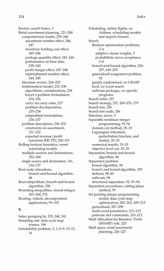
P1: Naresh

August 23, 2005 10:52 1914 1914˙Index

314 Index

Restart, search basics, 3Retail assortment planning, 221–248

computational results, 239–248assortment number effect, 246,

247inventory holding cost effect,

245–246package quantity effect, 243–244performance on base data,

239–242profit margin effect, 247–248replenishment number effect,

244, 245literature review, 224–229mathematical model, 232–238

algorithmic considerations, 238buyer’s problem formulation,

234–236carry/no carry rules, 237problem decomposition,

233–234subproblem formulation,

236–237problem description, 230–232

constraints on assortment,231–232

expected revenue/profitfunctions (ER/PF), 230–231

Rolling horizon heuristics, vesselscheduling models

multiple sources and destinations,182–184

single source and destination, 141,154–157

Root node relaxations,branch-and-bound algorithm,48

Root subproblem, branch-and-boundalgorithm, 256

Rounding inequalities, mixed-integer,263–264, 274

Routing, vehicle, decompositionapplications, 99–103

S

Sales, grouping by, 235, 240, 241Sampling rate, data cycle map

frames, 198Satisfiability problem, 2, 3, 8–9, 13–15,

16

Scheduling, airline flights, seeAirlines, scheduling modelsand airport closures

SearchBoolean optimization problems,

3–6adaptive clause weights, 5probabilistic move acceptance,

5–6branch-and-bound algorithm, 256,

257, 269–270generalized assignment problem,

54greedy randomized, see GRASPlocal, see Local searchsoftware packages, see specific

programsSearch order, 257Search strategy, 257, 269–270, 275Search tree, 256Search tree node, 256Selection, move, 3Separable nonlinear integer

programming, 19–36domain cut method, 29–33Lagrangian relaxation,

perturbation function, andduality, 20–25

numerical results, 33–35objective level cut, 25–29

Separation, branch-and-boundalgorithm, 49

Separation problembound algorithm, 58branch and bound algorithm, 259defined, 58, 60software, 98structured separation, 92, 93–94

Separation procedures, cutting planemethod, 59

Set packing integer programmingmodel, data cycle mapoptimization, 202–203, 209–215

generalized, 207–209multi-word parameters, 212–215pairwise slot constraints, 210–212

Shelf Allocation for Retailers’ Profit(SHARP) rule, 225

Shelf space, retail assortmentplanning, 226–227

P1: Naresh

August 23, 2005 10:52 1914 1914˙Index

Index 315

Simple generalized flow coverinequality, 262

Simplex methods, 96Size, grouping by, 235, 240, 241,

242SKU (stock keeping units), see Retail

assortment planningSliding flights, airline, 113Slot constraints, set packing integer

programming model, datacycle map optimization,210–212

Software, 254–299benchmarking, 294–298branch-and-bound algorithm,

256–270branching, 266–269lower bounding methods,

258–265search strategy, 269–270upper bounding methods,

265–266case studies, 288–294

branch and cut, 288–291branch and price, 291–294

decomposition, 97–98future trends, 298–299generalized assignment problem,

52MILP programs

ABACUS, 275–277BCP, 277–279BonsaiG, 279–280CBC, 280–282GLPK, 282–283lp_solve, 283–284MINTO, 284–286SYMPHONY, 286–288

user interfaces, 270–273black-box solvers, 270–272callable libraries, 272–273solver frameworks, 273

Solver frameworks, user interfaces,273

Solversblack-box, 270–272user interfaces, 272

SOPLEX, 274SOS (special ordered sets), 268Special ordered sets (SOS), 268

Stabilization methods, masterproblem solution, 96–97

Starting solution, search basics, 3Static search strategies, 269Steiner tree problem, decomposition

applications, 105–107Stock keeping units (SKU), see Retail

assortment planningStopping criterion, search basics, 3Structured separation, 92, 93–94Subcommutation, data cycle map

frames, 198, 201, 202–203, 204Subgradient methods, 97Subproblem

branch-and-bound algorithm, 256decomposition

cutting, 92–96defined, 58synergy between, 59

formulation for retail assortmentplanning, 236–237

Subtour elimination constraints(SECs)

separating solutions with knownstructure, 93–94

Traveling Salesman Problem, 64Successive shortest path (SSP)

method, airline flights, 127,128, 131

Supercommutation, data cycle mapframes, 198, 201, 202, 203

SYMPHONY, 274, 277benchmarking, 296, 297, 298branch and cut case study, 288–291features of, 255, 286–288

T

Tabu search, 15–16Tabu tenure, 3Telemetry frames, see Data cycle map

optimizationTemplate paradigm, 92, 93Three-index assignment problem

branch and price case study,291–293

decomposition applications,103–105

Time-space networks, airlinemanagement, 113, 114–115

P1: Naresh

August 23, 2005 10:52 1914 1914˙Index

316 Index

Transport schedulingairline flights, see Airlines,

scheduling models and airportclosures

ocean vessels, see Vessel schedulingTraveling Salesman Problem, 62–64

multiple, 100, 102–103two-matching polyhedron and, 84

Two-matching problem, 84Two-matching solution, 88, 89Two-phase heuristic, retail

assortment planning, 226Two-phase search methods, 270

U

Upper boundsairline flights, 125–126branch-and-bound algorithm, 257branch-and-bound algorithm

software, 265–266generalized assignment problem,

methods for decreasing, 47–48generalized upper bound (GUB)

cover inequalities, 260–261software, see specific programs

User interfacesblack-box solvers, 270–272callable libraries, 272–273MILP software programs, see

specific programssolver frameworks, 273

V

Valid inequalities, see Inequalities,valid

Validity, marginal conditional, 7–8,10–12, 16

Vehicle routing problem,decomposition applications,99–103

Vessel schedulingmultiple sources and destinations,

168–193aggregated reformulation of

VSM, 178–182future research, 185–186model formulation, 174–178notation, glossary of, 187–191

problem description, 170–174problem statement, 168related research, 168–170rolling horizon algorithm,

182–184test problems, 191–193usefulness of modeling

approach, 185single source and destination,

137–160aggregate formulation AVSM for

model VSM, 150–153comparison with ad hoc

scheduling, 157–159computational results, 153–154future research, 159–160literature, 139–143model constraints, 147–148model formulation, overall,

149–150model variables, 146–147objective function, 148penalty functions, 144–145problem description, 137–139problem notation and

assumptions, 143–144rolling horizon heuristics,

154–157Violated GSEC, 100–102Violated inequalities, price and cut,

85, 89Visual C++, 287Volume algorithm, 92

W

Weighted maximum satisfiability,Boolean optimizationproblems, 2, 8–9, 13–15, 16

Wrapper function, SYMPHONY, 287

X

XML (extensible markup language),271

XPRESS, 16, 255XPRESS-MP, 274, 285

Z

ZIMPL, 271

Integer Programming : Theory and Practice

Documents

Transcript of Integer Programming : Theory and Practice