Integer programming for locating ambulances

Laura Albert McLay

The Industrial & Systems Engineering Department

University of Wisconsin-Madison

laura@engr.wisc.edu

punkrockOR.wordpress.com

@lauramclay

1This work was in part supported by the U.S. Department of the Army under Grant Award Number W911NF-10-1-0176 and

by the National Science Foundation under Award No. CMMI -1054148, 1444219.

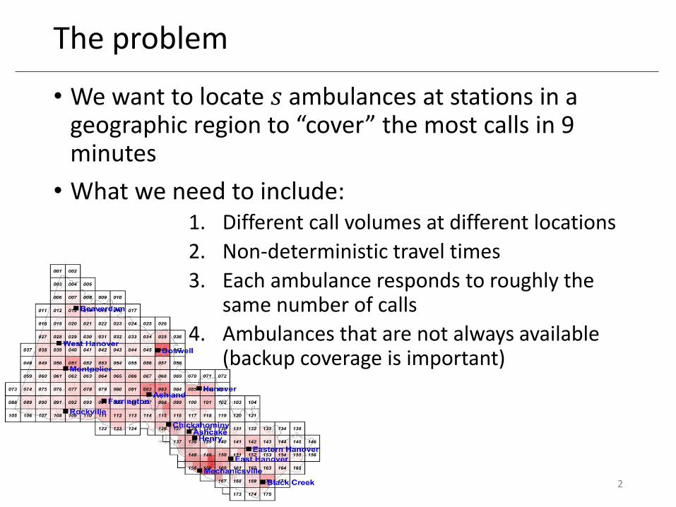
The problem

• We want to locate 𝑠 ambulances at stations in a geographic region to “cover” the most calls in 9 minutes

• What we need to include:1. Different call volumes at different locations

2. Non-deterministic travel times

3. Each ambulance responds to roughly the same number of calls

4. Ambulances that are not always available (backup coverage is important)

2

The solution:

3

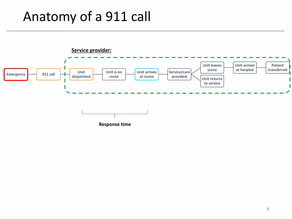
Anatomy of a 911 call

Response time

Service provider:

Emergency 911 callUnit

dispatchedUnit is en

routeUnit arrives

at sceneService/care

provided

Unit leaves scene

Unit arrives at hospital

Patient transferred

Unit returns to service

4

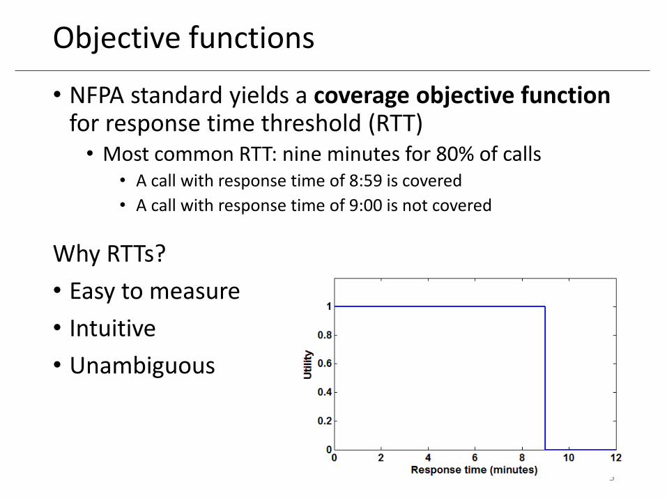
Objective functions

• NFPA standard yields a coverage objective function for response time threshold (RTT)• Most common RTT: nine minutes for 80% of calls

• A call with response time of 8:59 is covered

• A call with response time of 9:00 is not covered

Why RTTs?

• Easy to measure

• Intuitive

• Unambiguous

5

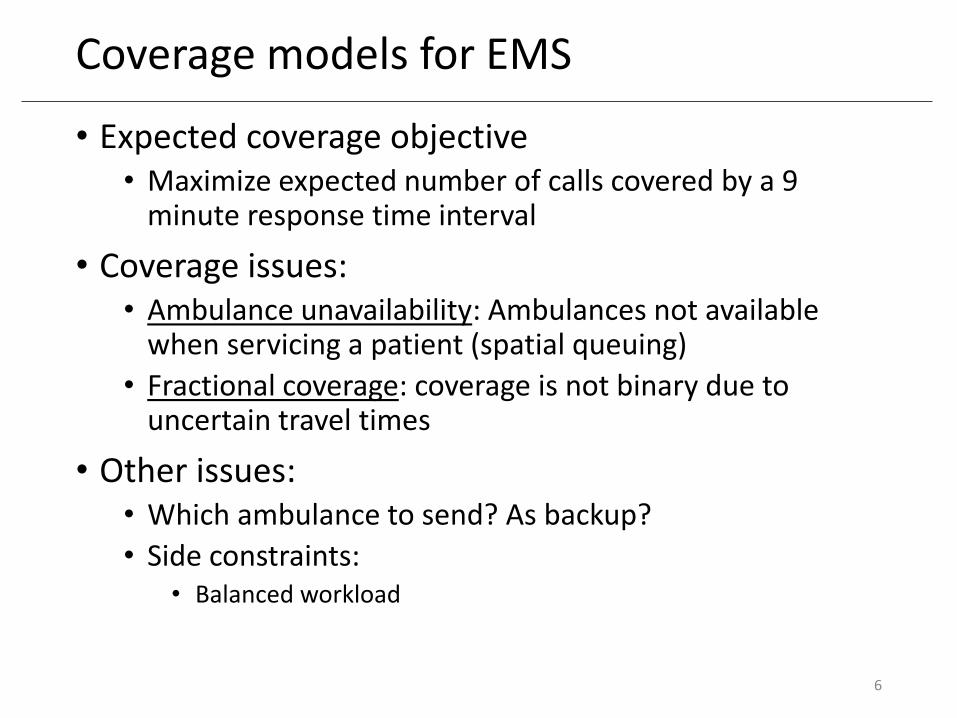
Coverage models for EMS

• Expected coverage objective• Maximize expected number of calls covered by a 9

minute response time interval

• Coverage issues:• Ambulance unavailability: Ambulances not available

when servicing a patient (spatial queuing)

• Fractional coverage: coverage is not binary due to uncertain travel times

• Other issues:• Which ambulance to send? As backup?

• Side constraints:• Balanced workload

6

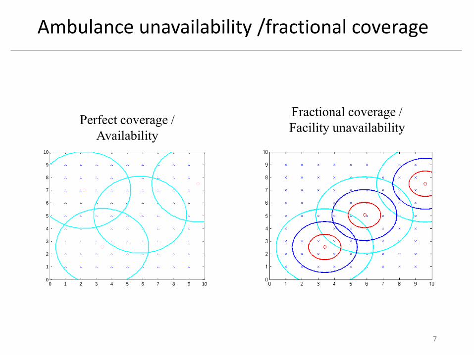
Ambulance unavailability /fractional coverage

7

Fractional coverage /

Facility unavailability

0 1 2 3 4 5 6 7 8 9 100

1

2

3

4

5

6

7

8

9

10

Perfect coverage /

Availability

Why use optimization models?

Because it helps you identify solutions that are not intuitive. This adds value!

8

MODEL

Model 1: covering location modelsAdjusts for different call volumes at different locations (#1), but does not include our other needs

9

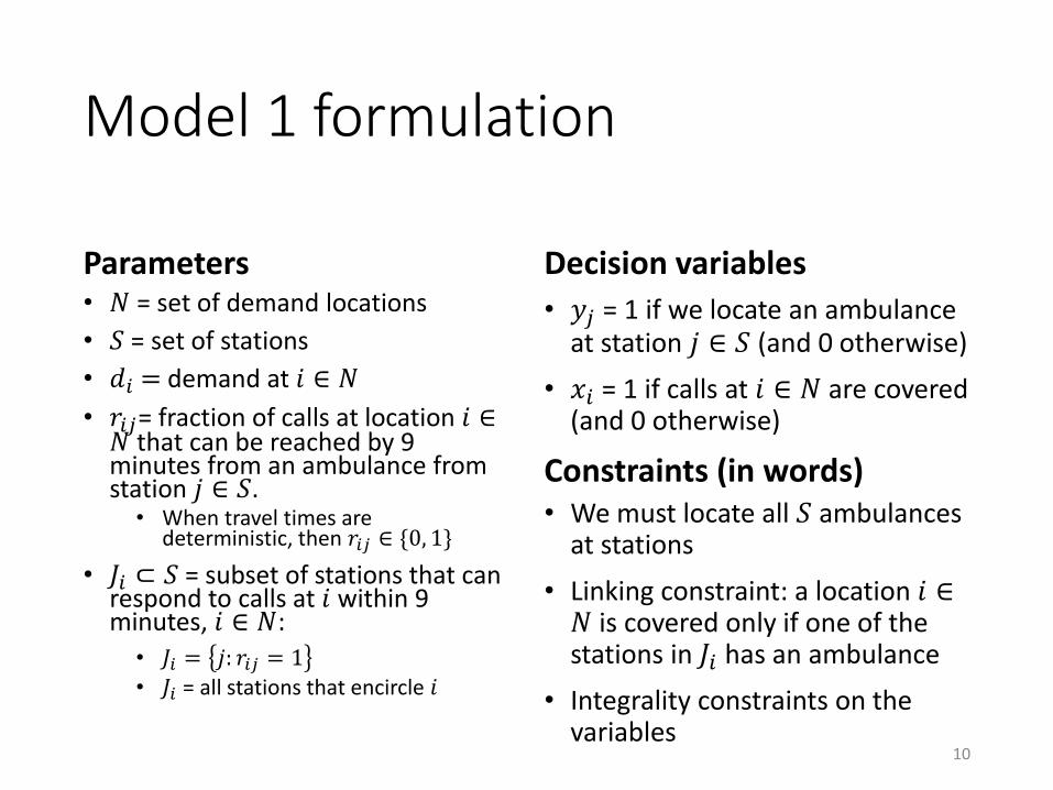
Model 1 formulation

Parameters• 𝑁 = set of demand locations

• 𝑆 = set of stations

• 𝑑𝑖 = demand at 𝑖 ∈ 𝑁

• 𝑟𝑖𝑗= fraction of calls at location 𝑖 ∈𝑁 that can be reached by 9 minutes from an ambulance from station 𝑗 ∈ 𝑆.

• When travel times are deterministic, then 𝑟𝑖𝑗 ∈ {0, 1}

• 𝐽𝑖 ⊂ 𝑆 = subset of stations that can respond to calls at 𝑖 within 9 minutes, 𝑖 ∈ 𝑁:

• 𝐽𝑖 = 𝑗: 𝑟𝑖𝑗 = 1

• 𝐽𝑖 = all stations that encircle 𝑖

Decision variables

• 𝑦𝑗 = 1 if we locate an ambulance at station 𝑗 ∈ 𝑆 (and 0 otherwise)

• 𝑥𝑖 = 1 if calls at 𝑖 ∈ 𝑁 are covered (and 0 otherwise)

• We must locate all 𝑆 ambulances at stations

• Linking constraint: a location 𝑖 ∈𝑁 is covered only if one of the stations in 𝐽𝑖 has an ambulance

• Integrality constraints on the variables

10

Constraints (in words)

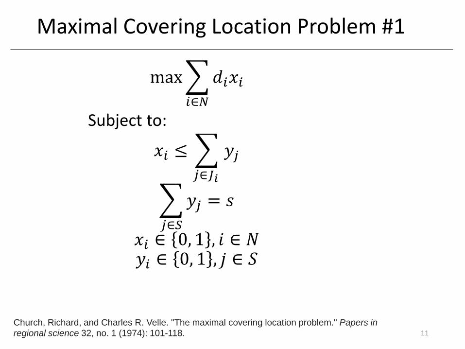
Maximal Covering Location Problem #1

max

𝑖∈𝑁

𝑑𝑖𝑥𝑖

Subject to:

𝑥𝑖 ≤

𝑗∈𝐽𝑖

𝑦𝑗

𝑗∈𝑆

𝑦𝑗 = 𝑠

𝑥𝑖 ∈ 0, 1 , 𝑖 ∈ 𝑁𝑦𝑖 ∈ 0, 1 , 𝑗 ∈ 𝑆

11

Church, Richard, and Charles R. Velle. "The maximal covering location problem." Papers in

regional science 32, no. 1 (1974): 101-118.

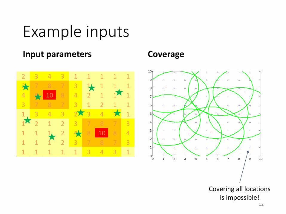
Example inputsInput parameters Coverage

12

0 1 2 3 4 5 6 7 8 9 100

1

2

3

4

5

6

7

8

9

10

Covering all locations is impossible!

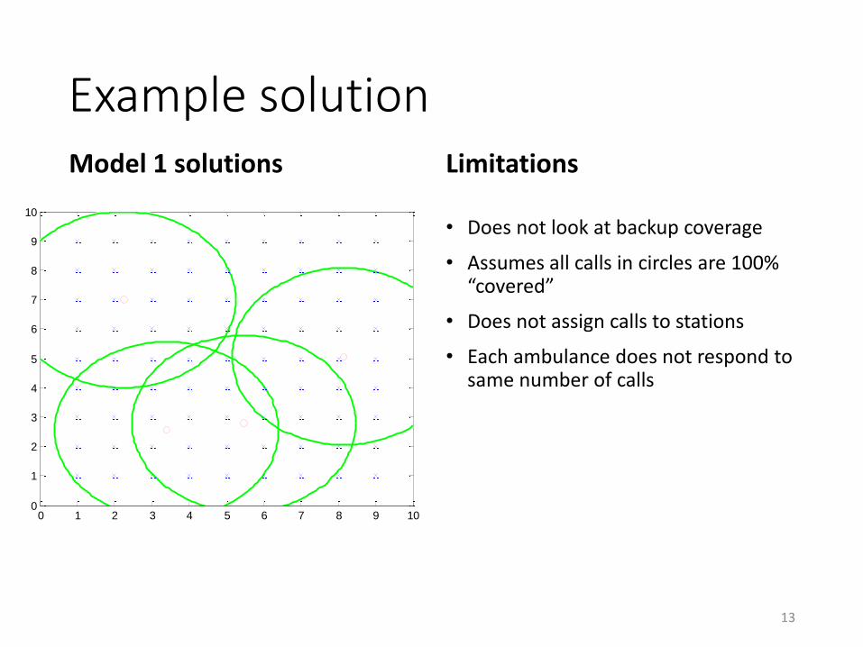
Example solutionModel 1 solutions

0 1 2 3 4 5 6 7 8 9 100

1

2

3

4

5

6

7

8

9

10

Limitations

13

• Does not look at backup coverage

• Assumes all calls in circles are 100% “covered”

• Does not assign calls to stations

• Each ambulance does not respond to same number of calls

Model 2: p-median models to maximize expected coverageAddresses:

1. Different call volumes at different locations

2. Non-deterministic travel times

3. Each ambulance responds to roughly the same number of calls

Does not address #4: backup coverage14

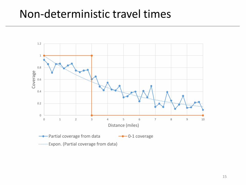
Non-deterministic travel times

15

0

0.2

0.4

0.6

0.8

1

1.2

0 1 2 3 4 5 6 7 8 9 10

Co

vera

ge

Distance (miles)

Partial coverage from data 0-1 coverage

Expon. (Partial coverage from data)

Let’s extend our formulation

16

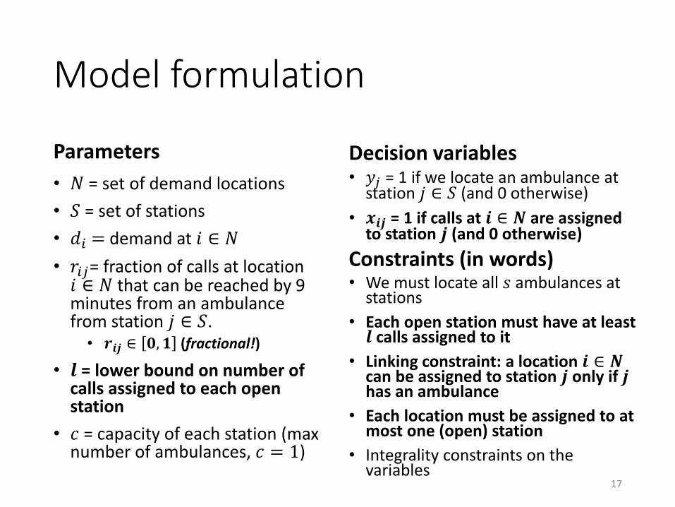
Model formulation

Parameters

• 𝑁 = set of demand locations

• 𝑆 = set of stations

• 𝑑𝑖 = demand at 𝑖 ∈ 𝑁

• 𝑟𝑖𝑗= fraction of calls at location 𝑖 ∈ 𝑁 that can be reached by 9 minutes from an ambulance from station 𝑗 ∈ 𝑆.

• 𝒓𝒊𝒋 ∈ 𝟎, 𝟏 (fractional!)

• 𝒍 = lower bound on number of calls assigned to each open station

• 𝑐 = capacity of each station (max number of ambulances, 𝑐 = 1)

Decision variables• 𝑦𝑗 = 1 if we locate an ambulance at

station 𝑗 ∈ 𝑆 (and 0 otherwise)

• 𝒙𝒊𝒋 = 1 if calls at 𝒊 ∈ 𝑵 are assigned to station 𝒋 (and 0 otherwise)

• We must locate all 𝑠 ambulances at stations

• Each open station must have at least 𝒍 calls assigned to it

• Linking constraint: a location 𝒊 ∈ 𝑵can be assigned to station 𝒋 only if 𝒋has an ambulance

• Each location must be assigned to at most one (open) station

• Integrality constraints on the variables

17

Constraints (in words)

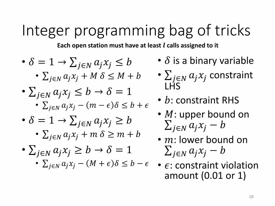
Integer programming bag of tricks

• 𝛿 = 1 → 𝑗∈𝑁 𝑎𝑗𝑥𝑗 ≤ 𝑏

• 𝑗∈𝑁 𝑎𝑗𝑥𝑗 +𝑀 𝛿 ≤ 𝑀 + 𝑏

• 𝑗∈𝑁 𝑎𝑗𝑥𝑗 ≤ 𝑏 → 𝛿 = 1• 𝑗∈𝑁 𝑎𝑗𝑥𝑗 − 𝑚 − 𝜖 𝛿 ≤ 𝑏 + 𝜖

• 𝛿 = 1 → 𝑗∈𝑁 𝑎𝑗𝑥𝑗 ≥ 𝑏

• 𝑗∈𝑁 𝑎𝑗𝑥𝑗 +𝑚 𝛿 ≥ 𝑚 + 𝑏

• 𝑗∈𝑁 𝑎𝑗𝑥𝑗 ≥ 𝑏 → 𝛿 = 1• 𝑗∈𝑁 𝑎𝑗𝑥𝑗 − 𝑀 + 𝜖 𝛿 ≤ 𝑏 − 𝜖

• 𝛿 is a binary variable

• 𝑗∈𝑁 𝑎𝑗𝑥𝑗 constraint LHS

• 𝑏: constraint RHS

• 𝑀: upper bound on 𝑗∈𝑁 𝑎𝑗𝑥𝑗 − 𝑏

• 𝑚: lower bound on 𝑗∈𝑁 𝑎𝑗𝑥𝑗 − 𝑏

• 𝜖: constraint violation amount (0.01 or 1)

18

Each open station must have at least 𝒍 calls assigned to it

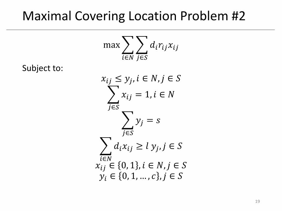
Maximal Covering Location Problem #2

max

𝑖∈𝑁

𝑗∈𝑆

𝑑𝑖𝑟𝑖𝑗𝑥𝑖𝑗

Subject to:𝑥𝑖𝑗 ≤ 𝑦𝑗 , 𝑖 ∈ 𝑁, 𝑗 ∈ 𝑆

𝑗∈𝑆

𝑥𝑖𝑗 = 1, 𝑖 ∈ 𝑁

𝑗∈𝑆

𝑦𝑗 = 𝑠

𝑖∈𝑁

𝑑𝑖𝑥𝑖𝑗 ≥ 𝑙 𝑦𝑗 , 𝑗 ∈ 𝑆

𝑥𝑖𝑗 ∈ 0, 1 , 𝑖 ∈ 𝑁, 𝑗 ∈ 𝑆𝑦𝑖 ∈ 0, 1,… , 𝑐 , 𝑗 ∈ 𝑆

19

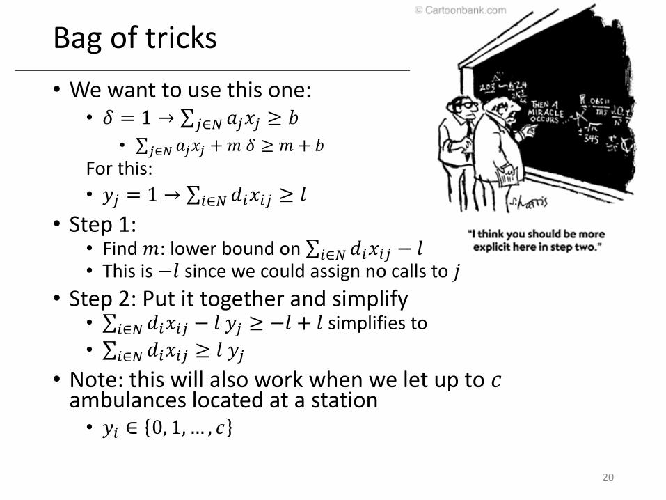
Bag of tricks

• We want to use this one:• 𝛿 = 1 → 𝑗∈𝑁 𝑎𝑗𝑥𝑗 ≥ 𝑏

• 𝑗∈𝑁 𝑎𝑗𝑥𝑗 +𝑚 𝛿 ≥ 𝑚 + 𝑏

For this:

• 𝑦𝑗 = 1 → 𝑖∈𝑁 𝑑𝑖𝑥𝑖𝑗 ≥ 𝑙

• Step 1:• Find 𝑚: lower bound on 𝑖∈𝑁 𝑑𝑖𝑥𝑖𝑗 − 𝑙• This is −𝑙 since we could assign no calls to 𝑗

• Step 2: Put it together and simplify• 𝑖∈𝑁 𝑑𝑖𝑥𝑖𝑗 − 𝑙 𝑦𝑗 ≥ −𝑙 + 𝑙 simplifies to

• 𝑖∈𝑁 𝑑𝑖𝑥𝑖𝑗 ≥ 𝑙 𝑦𝑗

• Note: this will also work when we let up to 𝑐ambulances located at a station• 𝑦𝑖 ∈ 0, 1, … , 𝑐

20

0 1 2 3 4 5 6 7 8 9 100

1

2

3

4

5

6

7

8

9

10

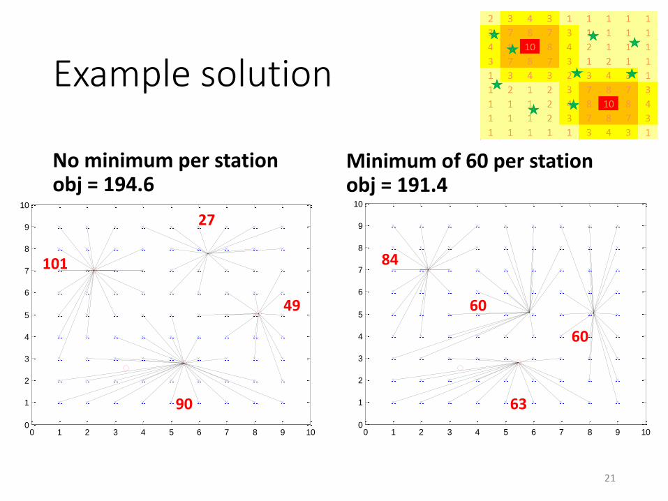
Example solution

No minimum per stationobj = 194.6

0 1 2 3 4 5 6 7 8 9 100

1

2

3

4

5

6

7

8

9

10

Minimum of 60 per stationobj = 191.4

21

101

49

27

90

60

84

60

63

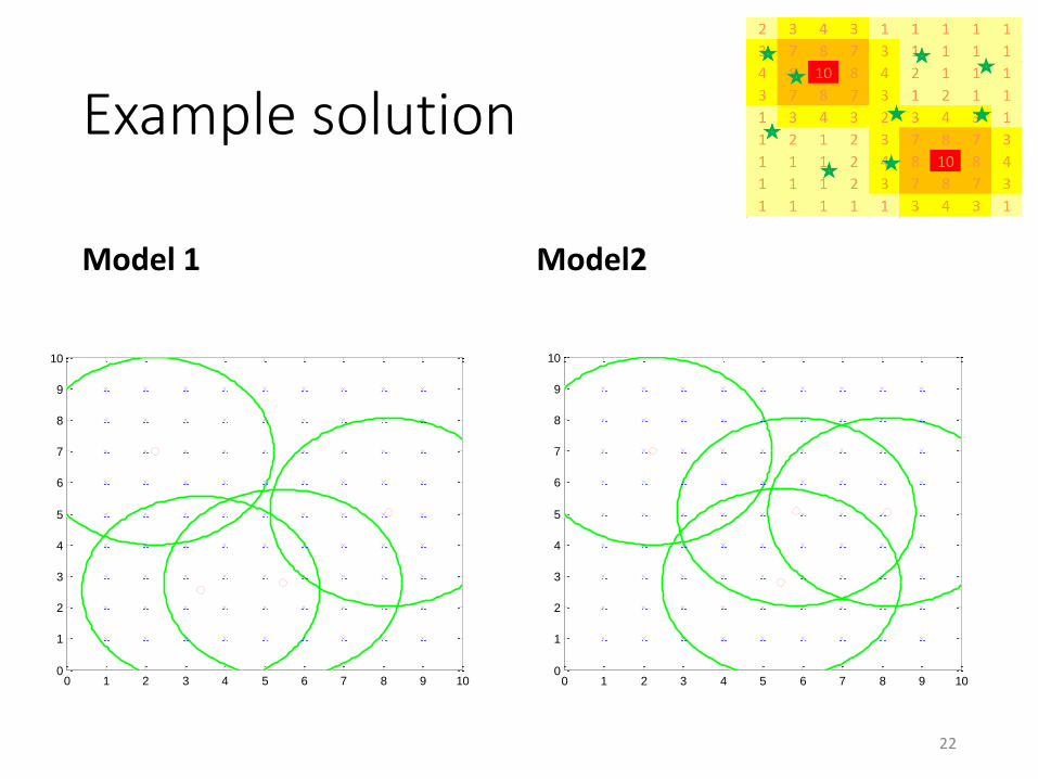
Example solution

Model 1

0 1 2 3 4 5 6 7 8 9 100

1

2

3

4

5

6

7

8

9

10

Model2

0 1 2 3 4 5 6 7 8 9 100

1

2

3

4

5

6

7

8

9

10

22

Model 3: p-median models to maximize expected (backup) coverageAddresses:

1. Different call volumes at different locations

2. Non-deterministic travel times

3. Each ambulance responds to roughly the same number of calls

4. Ambulances that are not always available (backup coverage is important)

23

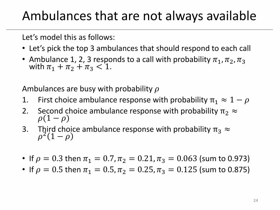
Ambulances that are not always available

Let’s model this as follows:

• Let’s pick the top 3 ambulances that should respond to each call

• Ambulance 1, 2, 3 responds to a call with probability 𝜋1, 𝜋2, 𝜋3with 𝜋1 + 𝜋2 + 𝜋3 < 1.

Ambulances are busy with probability 𝜌

1. First choice ambulance response with probability π1 ≈ 1 − 𝜌

2. Second choice ambulance response with probability π2 ≈𝜌(1 − 𝜌)

3. Third choice ambulance response with probability π3 ≈𝜌2 1 − 𝜌

• If 𝜌 = 0.3 then 𝜋1 = 0.7, 𝜋2 = 0.21, 𝜋3 = 0.063 (sum to 0.973)

• If 𝜌 = 0.5 then 𝜋1 = 0.5, 𝜋2 = 0.25, 𝜋3 = 0.125 (sum to 0.875)

24

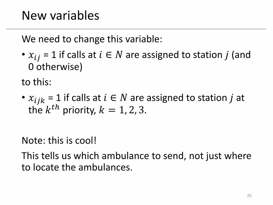
New variables

We need to change this variable:

• 𝑥𝑖𝑗 = 1 if calls at 𝑖 ∈ 𝑁 are assigned to station 𝑗 (and 0 otherwise)

to this:

• 𝑥𝑖𝑗𝑘 = 1 if calls at 𝑖 ∈ 𝑁 are assigned to station 𝑗 at the 𝑘𝑡ℎ priority, 𝑘 = 1, 2, 3.

Note: this is cool!

This tells us which ambulance to send, not just where to locate the ambulances.

25

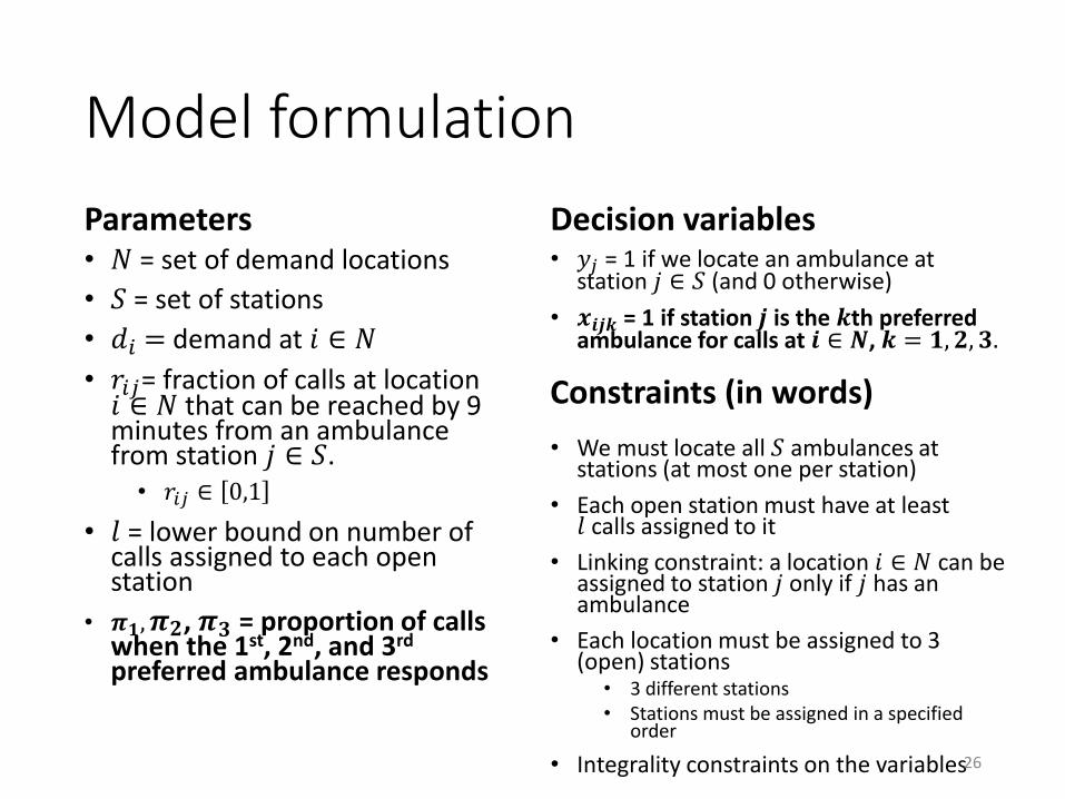
Model formulation

Parameters• 𝑁 = set of demand locations

• 𝑆 = set of stations

• 𝑑𝑖 = demand at 𝑖 ∈ 𝑁

• 𝑟𝑖𝑗= fraction of calls at location 𝑖 ∈ 𝑁 that can be reached by 9 minutes from an ambulance from station 𝑗 ∈ 𝑆.

• 𝑟𝑖𝑗 ∈ 0,1

• 𝑙 = lower bound on number of calls assigned to each open station

• 𝝅𝟏,𝝅𝟐, 𝝅𝟑 = proportion of calls when the 1st, 2nd, and 3rd

preferred ambulance responds

Decision variables• 𝑦𝑗 = 1 if we locate an ambulance at

station 𝑗 ∈ 𝑆 (and 0 otherwise)

• 𝒙𝒊𝒋𝒌 = 1 if station 𝒋 is the 𝒌th preferred ambulance for calls at 𝒊 ∈ 𝑵, 𝒌 = 𝟏, 𝟐, 𝟑.

• We must locate all 𝑆 ambulances at stations (at most one per station)

• Each open station must have at least 𝑙 calls assigned to it

• Linking constraint: a location 𝑖 ∈ 𝑁 can be assigned to station 𝑗 only if 𝑗 has an ambulance

• Each location must be assigned to 3 (open) stations

• 3 different stations• Stations must be assigned in a specified

order

• Integrality constraints on the variables26

Constraints (in words)

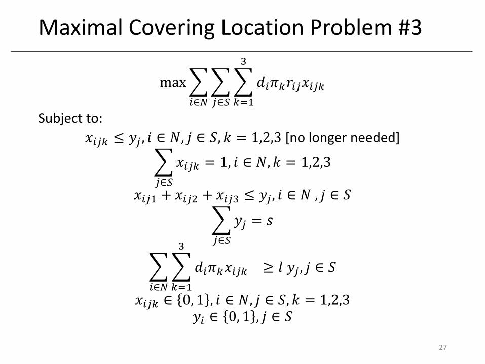
Maximal Covering Location Problem #3

max

𝑖∈𝑁

𝑗∈𝑆

𝑘=1

3

𝑑𝑖𝜋𝑘𝑟𝑖𝑗𝑥𝑖𝑗𝑘

Subject to:

𝑥𝑖𝑗𝑘 ≤ 𝑦𝑗 , 𝑖 ∈ 𝑁, 𝑗 ∈ 𝑆, 𝑘 = 1,2,3 [no longer needed]

𝑗∈𝑆

𝑥𝑖𝑗𝑘 = 1, 𝑖 ∈ 𝑁, 𝑘 = 1,2,3

𝑥𝑖𝑗1 + 𝑥𝑖𝑗2 + 𝑥𝑖𝑗3 ≤ 𝑦𝑗 , 𝑖 ∈ 𝑁 , 𝑗 ∈ 𝑆

𝑗∈𝑆

𝑦𝑗 = 𝑠

𝑖∈𝑁

𝑘=1

3

𝑑𝑖𝜋𝑘𝑥𝑖𝑗𝑘 ≥ 𝑙 𝑦𝑗 , 𝑗 ∈ 𝑆

𝑥𝑖𝑗𝑘 ∈ 0, 1 , 𝑖 ∈ 𝑁, 𝑗 ∈ 𝑆, 𝑘 = 1,2,3𝑦𝑖 ∈ 0, 1 , 𝑗 ∈ 𝑆

27

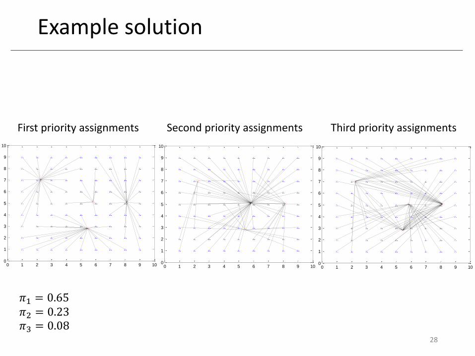
Example solution

0 1 2 3 4 5 6 7 8 9 100

1

2

3

4

5

6

7

8

9

10

28

0 1 2 3 4 5 6 7 8 9 100

1

2

3

4

5

6

7

8

9

10

0 1 2 3 4 5 6 7 8 9 100

1

2

3

4

5

6

7

8

9

10

First priority assignments Second priority assignments Third priority assignments

𝜋1 = 0.65𝜋2 = 0.23𝜋3 = 0.08

Related blog posts

• A YouTube video about my research

• In defense of model simplicity

• Operations research, disasters, and science communication

• Domino optimization art

29