Int. Workshop on the Foundations ofSpreadsheets (FOS’04)

Rome, ItalySeptember 30th, 2004

http://eecs.oregonstate.edu/˜erwig/FOS/

Int. Workshop on the Foundations ofSpreadsheets (FOS’04)

Program Committee

Alan Blackwell University of Cambridge, UKMargaret Burnett Oregon State University, USAMartin Erwig Oregon State University, USA (chair)Shriram Krishnamurthi Brown University, USAClayton Lewis University of Colorado, USASimon Peyton Jones Microsoft Research, Cambridge, UKJorma Sajaniemi University of Joensuu, FinlandSusan Wiedenbeck Drexel University, USA

I. Position Statements

Towards Safer Spreadsheets!

Robin AbrahamSchool of Electrical Engineering and Computer Science

Oregon State UniversityCorvallis, Oregon 97331, USA.

1 Introduction

Professional programmers are well aware that de-bugging, testing, code inspection, etc. are part andparcel of software development. Requiring end users tocarry out the same activities to reduce spreadsheet er-rors might be asking too much. For one thing, they lackthe expertise and for another, they might not be willingto invest the time and effort required by these activi-ties. For example, testing is a standard and effectivetechnique for detecting faults in programs. The down-side is that testing requires reasonable domain knowl-edge (to come up with effective test cases at the veryleast) and understanding of the program. End usersmight be deficient in one or both areas. Another prob-lem arises from the lack of tool support for runningtest suites in currently available commercial spread-sheet systems. This forces users to run one test at atime, thereby taking up more time.

2 Program Generator for Spreadsheets

We have developed a system that allows the user tocreate specifications that describe the structure of theinitial spreadsheet [2]. The system (named Gencel)translates the specification into the initial spreadsheetinstance and also generates customized update opera-tions (insert/delete operations for rows and columns)for the given specification. This approach guaranteesthat a spreadsheet instance generated by applicationof any sequence of the update operations to the initialspreadsheet instance conforms to the user-defined spec-ification. Moreover, given that the initial specificationis type-correct, any spreadsheet instance generated bythe application of the customized update operations isguaranteed to be free from omission, reference, or typeerrors.

∗This work is supported by the National Science Foundationunder the grant ITR-0325273 and by the EUSES Consortium(http://eecs.oregonstate.edu/EUSES/).

One concern that might arise about this approachis that it could detract from the flexibility offered byspreadsheet systems because of the constraints imposedon the update operations. We believe that the advan-tages will outweigh the intial investment (in trainingand creation of the initial specifications) because of thehuge savings in debugging and testing effort—the useronly needs to audit the initial specification and the datavalues entered in the generated instances.

To support the wide-spread adoption of the Gencelsystem, we need tools that allow the user to extract thespecifications from arbitrary spreadsheets. We plan touse some of the spatial analyses techniques developedin [1] to help with this task.

3 Conclusion

Most of the current approaches are aimed at help-ing end users detect errors in spreadsheets they havealready created. Programming language environmentsused in commercial software development employ sim-ple (syntax highlighting, auto completion) to sophisti-cated (type checkers, program generators) techniquesto prevent the incidence of errors in programs. Thismakes a strong case in favor of systems that help theusers create correct spreadsheets. In this context, webelieve that the Gencel approach is a big step towardsthe prevention of errors in spreadsheets.

References

[1] R. Abraham and M. Erwig. Header and Unit Inferencefor Spreadsheets Through Spatial Analyses. In IEEESymp. on Visual Languages and Human-Centric Com-puting, 2004.

[2] M. Erwig, R. Abraham, I. Cooperstein, and S. Koll-mansberger. Gencel — A Program Generator forCorrect Spreadsheets. Technical Report TR04-60-11,School of EECS, Oregon State University, 2004.

1

!"#$%&'#()*"##+$(*$($,*#'$-.+#'/(0#$

!"#$%&"#'()*""%

%

+,*%-./01%02/*#30,**1%)#0%#%04''*00%5*'#40*%.1%2/67.3*3%#%$*)%40*/%*82*/.*$'*9%$61%5*'#40*%6-%#$:%

'6$1*;26/#/:%1,*6/.*0%.$%,4;#$%'6;241*/%.$1*/#'1.6$%<6/%.$%'6;241.$=9%3*02.1*%#%2/.6/%2#1*$1%6-%

),.',%&/.'(".$%#$3%>/#$(016$%)*/*%4$#)#/*%?%@#11*00.',%ABCDEF%G1%.0%40*-4"%16%'6$0.3*/%,6)%#$3%

),:%H.0.I#"'%)#0%3.--*/*$1%16%1,*%/*0*#/',%#=*$3#%.$%JIG%#1%1,*%1.;*9%,6)%.10%04''*00%)#0%

0450*K4*$1":%/#1.6$#".0*39%#$3%),#1%#37#$'*0%,#7*%5**$%;#3*%.$%1,*%40#5.".1:%6-%02/*#30,**10%

0.$'*%1,*$F%

@601%JIG%/*0*#/',%.$%1,*%"#1*%ABLM0%)#0%01.""%'6$1.$4.$=%3./*'1.6$0%6/.=.$#"":%;61.7#1*3%5:%

;.".1#/:%/*0*#/',%1,/64=,%N.'(".3*/9%O41,*/"#$3%#$3%+#:"6/P0%3./*'16/0,.20%6-%1,*%!QR!%

G$-6/;#1.6$%R/6'*00.$=%+*',$.K4*0%S--.'*F%T*)%.$1*/#'1.6$%2#/#3.=;0%)*/*%'"*#/":%3*/.7*3%

*.1,*/%-/6;%O!UV%'6;;#$3%#$3%'6$1/6"%0'*$#/.609%6/%-/6;%I!W%-6/%#*/602#'*%;63*"".$=%#$3%

;#',.$*%166".$=F%V$=*"5#/1%#3621*3%1,*%;6/*%,4;#$.01.'%7.0.6$%6-%&40,P0%@*;*89%541%3*7*"62*3%

.1%.$%1,*%;.".1#/:%/*0*#/',%#1;602,*/*%6-%!QR!TV+F%G$%'6$1/#019%X#:P0%/#3.'#"%24/04.1%6-%#$%

*34'#1.6$#"%#=*$3#%-/6;%R#2*/1%*;2,#0.0*3%'/*#1.7*%*82"6/#1.6$%/#1,*/%1,#$%'6$7*$1.6$#"%".1*/#':%

#$3%$4;*/#':F%T6$*%6-%1,*0*%01/#$30%6-%/*0*#/',%=#7*%'"60*%'6$0.3*/#1.6$%16%540.$*00%'6;241.$=%

$**309%5*:6$3%1,*%#$63:$*%'6;;*/'.#".0#1.6$%6-%TNO%YZOGYZU%36'4;*$1#1.6$%-#'.".1.*0%.$16%

)6/3%2/6'*006/0F%

H.0.I#"'%)#0%3*7*"62*3%.$%.06"#1.6$%-/6;%1,.0%/*0*#/',%*$7./6$;*$1%.$%),.',%1,*%'6$'*210%6-%

[3./*'1%;#$.24"#1.6$\%#$3%[;*1#2,6/\%)*/*%=#.$.$=%'4//*$':F%&/.'(".$P0%6/.=.$#"%'6$'*21%)#0%

2/6161:2*3%.$%&!OGI%</*01/.'1*3%16%-.7*%'6"4;$0%5:%]M%/6)0E9%).1,%1,*%7.0.6$%6-%'/*#1.$=%#$%

[*"*'1/6$.'%5"#'(56#/3\F%G1%)#0%1#/=*1*3%#1%1,*%2"#1-6/;%1,#1%)#0%'"60*01%16%#%['6;;63.1:\%RI%?%

1,*%!22"*%GG%?%6$%1,*%#37.'*%6-%#%-64$3.$=%*3.16/%-/6;%&:1*%;#=#^.$*9%#$3%>/#$0(016$%621.;.0*3%

.1%16%/4$%-#01%.$%6$":%]MX%6-%;*;6/:F%

N#1*/%3*7*"62*/0%3.3%".11"*%16%',#$=*%1,.0%5#0.'%2#/#3.=;9%541%#3621*3%;6/*%-*#14/*0%1,#1%,#3%

5*'6;*%-#;.".#/%-/6;%)6/(%#1%R!QI%#$3%!22"*F%N6140%A_]_`%#33*3%2/*0*$1#1.6$%-*#14/*0%04',%#0%

',#/10%#$3%2"6109%#0%)*""%#0%3#1#5#0*%'#2#5.".1.*09%#-1*/%X#26/%,#3%2/*7.640":%3*7*"62*3%0.;."#/%

*81*$0.6$0%-6/%H.0.I#"'F%V8'*"%)#0%)/.11*$%5:%@.'/606-1%-6/%1,*%aA]X%@#'.$160,%.$%ABbDF%G1%

2/67.3*3%24""_36)$%;*$40%#$3%;640*%26.$1.$=%<#$3%)#0%1,*%-"#=0,.2%#22".'#1.6$%-6/%Y.$36)0%

`FMEF%

JIG%/,*16/.'%6-%1,*%ABbMP0%'"#.;*3%1,#1%02/*#30,**10%)*/*%[$#14/#"\%5*'#40*%6-%1,*%#3621.6$%6-%#%

)*""_',60*$%;*1#2,6/9%#0%).1,%61,*/%[3*0(162\%-*#14/*0F%G$%-#'19%1,*%;*1#2,6/%)#0%;.$.;#"F%@6/*%

;4$3#$*%-*#14/*0%)*/*%1,*%-#'1%1,#1%-*)%61,*/%#22".'#1.6$0%6/=#$.0*3%3#1#%2/62*/":%.$16%'6"4;$09%

#$3%;601%'#"'4"#16/0%(*21%$6%/*'6/3%6-%2/*7.640%'#"'4"#1.6$0%?%561,%-*#14/*0%1,#1%#/*%*00*$1.#"%.$%

566(_(**2.$=F%O450*K4*$1%02/*#30,**10%)*/*%04''*00-4"%16%1,*%*81*$1%1,#1%1,*:%2/*0*/7*3%1,*0*%

*00*$1.#"%-*#14/*0F%@:%1#"(%).""%'6$0.3*/%,6)%.$$67#1.6$0%.$%1,*%02/*#30,**1%2#/#3.=;%'#$%5*%

3*0.=$*3%#$3%#00*00*3%.$%1,*%".=,1%6-%1,*0*%'/.1.'#"%#11/.541*0F%

%N*7:9%OF%<ABBDEF%G$0#$*":%=/*#1c%+,*%".-*%#$3%1.;*0%6-%@#'.$160,9%1,*%I6;241*/%1,#1%',#$=*3%*7*/:1,.$=F%

N6$36$c%R*$=4.$%

@#11*00.',9%QF%<ABCDEF%O.;4"#1.6$%6-%1,*%-./;%1,/64=,%#%543=*1%'6;241*/%2/6=/#;F%G/).$F%

R6)*/9%WF%dF9%e!%&/.*-%J.016/:%6-%O2/*#30,**10e9%WOOQ*064/'*0FIS@9%Y6/"3%Y.3*%Y*59%

,112cff300/*064/'*0F'6;f,.016/:f00,.016/:F,1;"9%7*/0.6$%`FC9%Mbf`Mf]MMDF%

Q,*.$=6"39%JF%<]MMMEF%+66"0%-6/%1,64=,1c%+,*%,.016/:%#$3%-414/*%6-%;.$3_*82#$3.$=%1*',$6"6=:%<]$3%*3EF%

I#;5/.3=*9%@!c%@G+%R/*00%

O;.1,9%WFXF%#$3%!"*8#$3*/9%QFIF%<ABbbEF%>4;5".$=%1,*%-414/*c%J6)%g*/68%.$7*$1*39%1,*$%.=$6/*39%1,*%-./01%

2*/06$#"%'6;241*/F%T*)%Z6/(c%Y."".#;%@6//6)%

-

A Spreadsheet-Based View of the

End-User Software Engineering Concept1

Margaret Burnett, Curtis Cook and Gregg RothermelSchool of Electrical Engineering and Computer Science

Oregon State UniversityCorvallis, OR 97331 USA

{burnett, cook, grother}@eecs.orst.edu

End-user programming is arguably the most common form of programming in use today, but there has been little

investigation into the dependability of the programs end users create. Instead, most environments for end-user programming

support only programming. Giving end-user programmers ways to easily create their own programs is important, but it is not

enough. Like their counterparts in the world of professional software development, end-user programmers need support for

other aspects of the software lifecycle.

We have been investigating ways to address this problem by developing a software engineering paradigm viable for end-user

programming, an approach we call end-user software engineering. Because end users are different from professional

programmers in background, motivation and interest, the end user community cannot be served by simply repackaging

techniques and tools developed for professional software engineers. For this reason, end-user software engineering does not

mimic the traditional approaches of segregated support for each element of the software engineering life cycle, nor does it ask

the user to think in those terms. Instead, it employs a feedback loop supported by highly incremental testing, fault

localization heuristics, and deductive reasoning, which collaborate to help monitor dependability as the end user’s program

evolves. This approach helps guard against the introduction of faults in the user’s program and, if faults have already been

introduced, helps the user detect and locate them.

We have prototyped our approach in the spreadsheet paradigm. Our prototypes employ the following end-user software

engineering devices:

• Interactive, incremental systematic testing facilities.

• Interactive, incremental fault localization facilities.

• Interactive, collaborative assertion generation and propagation facilities.

• Motivational devices that gently attempt to interest end users in appropriate software engineering behaviors at

suitable moments.

We have conducted more than a dozen empirical studies related to this research, and the results have been very encouraging.

(More details about the studies are at http://www.engr.oregonstate.edu/~burnett/ITR2000/empirical.html.) Directly supporting

these users in software development activities beyond the programming stage—while at the same time taking their differences

in background, motivation, and interests into account—is the essence of the end-user software engineering vision.

For further reference:

M. Burnett, C. Cook, and G. Rothermel, “End-User Software Engineering,” Communications of the ACM, September 2004.

1 This work has been supported in part by NSF under ITR-0082265 and in part by the EUSES Consortium via NSF’s ITR-

0325273.

IEEE FOS (Foundations of Spreadsheets) Workshop

Rome September 30 2004

Position StatementPat Cleary

Researchers need a shift in perspective. End User Development (EUD), and in

particular the use of spreadsheets, is essentially an organisational issue, not a technical

one. We must understand organisations and how they behave. Organisations consist

of people interacting within some sort of structure. People are complex, far more

complex than we as technologists understand, and people in organisations are even

more complex. As such, the solutions to EUD problems are organisational not

technical. We need to understand the context in which EUD takes place. Why do

users choose to model a business process using a spreadsheet rather than some

alternative vehicle? If a decision-maker is forced through organisational policy to

adopt an alternative, is there likely to be a loss of motivation? The answers are likely

to lie in the domain of psychology rather than computing. Ray Panko (Panko 2003)

has been encouraging us to look outside our own disciplines to seek understanding

and knowledge to help our research. At UWIC, we are embarking on a programme of

research aimed at understanding spreadsheet use and then attempting to provide a

framework for risk reduction:

- Categorise spreadsheet use within an organisation according to some agreed

criteria e.g. an estimate of financial risk; complexity; number of potential

users; motivation of the modeller;

- For each category, formulate a strategy for risk reduction; this may vary from

do nothing (continue as before) to do not use spreadsheets for this category.

Between these two extremes of the continuum, a variety of strategies may use

the variety of tools and techniques already available or may demand new tools

to be developed.

- Implement the strategies and monitor the effect.

A number of issues need to be understood and resolved at this initial stage, e.g. how

do you measure spreadsheet use? In particular, how do you measure motivation/de-

motivation? Clearly, without a suitable metric(s), it is not going to be possible to

recognise success and failure.

Reference:

Panko, R. R., ‘Reducing Overconfidence in Spreadsheet Development’, Proceedings

of EuSpRIG Conference, Dublin, 2003

Foundations of Spreadsheets

Rome 2004

Position Statement by Grenville Croll

Background

By way of introduction, I should mention that as a young software engineer, I was responsible for

re-engineering Lotus 1-2-3 for the European marketplace, way back in 1984. I had the good

fortune to meet and work with Mitch Kapor, Jonathan Sachs and the software engineers who took

Lotus 1-2-3 through its early versions. Subsequently, for an unbroken period of nearly fifteen

years I ran a couple of small UK companies (4-5-6 World and Eastern Software Publishing),

developing and marketing Lotus and Excel add-ins and related training. The products provided

anything from basic functionality – graphics, function libraries and printer drivers – through to

more advanced technologies including Monte Carlo Simulation, Neural Networks and Linear

Programming. My present employer, Frontline Systems, was founded and is managed by Dan H.

Fylstra who previously founded Personal Computer Software, later renamed VisiCorp, publishers

of VisiCalc, the first mass market spreadsheet. Frontline Systems presently supply a diverse

range of optimisation software products for Microsoft Excel. For the last five years I have been

closely involved with the European Spreadsheet Risks Interest Group (EuSpRIG). At the

Amsterdam conference in 2001, I gave a presentation on the work of Mattesich, the originator of

the first electronic spreadsheet.

Frame Questions

HCI perspective. Given the 25 year history of spreadsheets, we can look forward with

considerable certainty to at least another 25 years of their business use in essentially their present

form. With this in mind, what set of five and ten year objectives might it be reasonable to aspire

to in order to positively influence the work and leisure lives of over 100 million spreadsheet users

over a period of this length?

Business Perspectives. We know almost nothing about how spreadsheets are used in business,

beyond our own experience – what are the uses of spreadsheets? We assume that we make better

business decisions using spreadsheets, but to what extent is this actually true? Can we identify

areas where spreadsheets should not be used and create or recommend a replacement? Are there

new areas where spreadsheets could be effectively deployed?

Programming perspective. An enduring theme through the life of spreadsheets has been the

desire to create and manipulate them programmatically, to compile them having been written

manually, then to decompile them automatically to assist in debugging. Can we conceive of and

implement a simple to use, integrated architecture that can achieve all this?

Quality Perspective. How can we continue to improve the educational process relating to

spreadsheets - from their active use in primary education through their role in the teaching of

quantum chemistry.

FOS’04 Workshop — Position Statement

Martin Erwig, Oregon State University

We believe the two most promising ways to improve reliability of spreadsheets are the development of:

• Automatic tools for error detection• Tools for automatically generating correct spreadsheets from specifications

The focus should be on automatic tools, because anything that has to be done “manually” in addition tocreating a spreadsheet takes time, which end users are reluctant to spend.

One promising approach to automatic error-detection tools is to define type systems that exploit thelabels and spatial structure of spreadsheets [6, 4, 2, 3, 1].

However, an even greater potential lies in the development of new programming approaches for spread-sheets. Existing spreadsheet systems work with a simple programming model of a flat collection of cells thatdo not contain any structure other than their arrangement on a grid. In particular, cells are identified byglobal row and column numbers (letters) so that references have to be expressed using these global addresses.This lack of structure puts current spreadsheet systems into the category of assembly languages when com-pared to the state of the art in other programming languages. This situation is peculiar because spreadsheetsystems are equipped with very sophisticated user interfaces offering many fancy features, which can distractfrom their intrinsic language limitations. The rigid, global addressing scheme makes computations vulnerableto changes in the structure of the spreadsheet—much like in the old days of assembly language programmingwhere the introduction of a new item into the memory could cause some references to become invalid.

Instead of revealing this low-level memory structure to the user, we believe that spreadsheets should bebuilt using higher-level abstractions, such as, tables, headers, and repeating blocks. Correspondingly, insteadof creating spreadsheets through arbitrary, uncontrolled cell manipulations, spreadsheets should be allowed toevolve only according to specification that describes the principal structure of the initial spreadsheet and all ofits future versions. Such a specification defines a schema or template for a spreadsheet that allows only thoseupdate operations that keep changed spreadsheets within the schema. A program generator can create fromthe specification an initial spreadsheet together with customized update operations for changing cells andinserting/deleting rows and columns for this particular specification [5]. These customized operations ensurethat the spreadsheet can be changed only into new versions that always adhere to the table specification. Atype system for specifications can guarantee that all spreadsheets that evolve through the customized updateoperations from a type-correct specification will never contain any reference, omission, or type errors.

References

[1] R. Abraham and M. Erwig. Header and Unit Inference for Spreadsheets Through Spatial Analyses. IEEESymp. on Visual Languages and Human-Centric Computing, 2004.

[2] Y. Ahmad, T. Antoniu, S. Goldwater, and S. Krishnamurthi. A Type System for Statically DetectingSpreadsheet Errors. 18th IEEE Int. Conf. on Automated Software Engineering, pp. 174–183, 2003.

[3] T. Antoniu, P. A. Steckler, S. Krishnamurthi, Neuwirth, and M. Felleisen. Validating the Unit Correctnessof Spreadsheet Programs. Int. Conf. on Software Engineering, 2004.

[4] M. M. Burnett and M. Erwig. Visually Customizing Inference Rules About Apples and Oranges. 2ndIEEE Int. Symp. on Human Centric Computing Languages and Environments, pp. 140–148, 2002.

[5] M. Erwig, R. Abraham, I. Cooperstein, and S. Kollmansberger. Gencel — A Program Generator forCorrect Spreadsheets. Technical Report TR04-60-11, School of EECS, Oregon State University, 2004.

[6] M. Erwig and M. M. Burnett. Adding Apples and Oranges. 4th Int. Symp. on Practical Aspects ofDeclarative Languages, LNCS 2257, pp. 173–191, 2002.

1

!"#$%&&'()*%$+',"-)$#'.%//0*10%*+'

2"134/)/%"$)-'."#0-5'"6'73*0)#5800/9:0;0-"310$/''

<=7>?>=@'7?A?B.B@?'

!

"#$%&'(!#)*(+,*-!./)'-'!0$1!2+&2!-11$1!1/(-'!+%!',1-/3'2--('4!*/.5!$0!,1$,-1!(1/+%+%&!/%3!

$0!3--,!)%3-1'(/%3+%&!$0!(2-!#$3-*!6-2+%3!',1-/3'2--(!.$#,)(/(+$%!/%3!3-7-*$,#-%(!+'!

%$(!(2-!*-/'(!/#$%&!(2-#8!92-!0/.(!(2/(!3-7-*$,+%&!',1-/3'2--('!+'!,1$&1/##+%&!/%3!(2)'!

%--3'! ,1$,-1! (1/+%+%&! '$#-2$:! .$%(1/3+.('! (2-! +%()+(+7-%-''! $0! 3-7-*$,+%&! '+#,*-!

',1-/3'2--('8! ;##-3+/(-! 0--36/.5! 1-,1-'-%(/(+$%! $0! 7/*)-'! $%*<4! (2-! ,$''+6+*+(<! ($! '2+0(!

.$#,*-=+(<!6<!',*+((+%&!0$1#)*/'!$7-1!3+00-1-%(!.-**'4!/%3!(2-!(/6)*/1!*/<$)(!2+3-!+%(1+./.<8!

92+'!+'!)'-0)*4!:2-%!:1+(+%&!/!',1-/3'2--(!,1$&1/#4!3+'()16+%&4!:2-%!(1<+%&!($!)%3-1'(/%3!

$1!#/+%(/+%!/!',1-/3'2--(8!!!

")3+(+%&!($$*'!2-*,!($!1-3).-!-11$1!1/(-'8!>)(4!,$:-10)*!/'!(2-<!/1-4!(2-<!/1-!-=,-1(!($$*'8!

?,1-/3'2--('4!(2$)&24!/1-!@)+(-!$0(-%!:1+((-%!6<!,-$,*-!:+(2!#+%+#/*!0$1#/*!',1-/3'2--(!

(1/+%+%&8!9$!,1$7+3-!(1/+%+%&!($!(2+'!.$##)%+(<!+%!/..-,(/6*<!'#/**!3$'-'4!+(!+'!+#,$1(/%(!

(2/(!+(!./%!1-'(!$%!/!'+#,*-!6)(!%-7-1(2-*-''!'$*+3!.$%.-,()/*!#$3-*8!92-!(21--!*/<-1'!$0!/!

',1-/3'2--(! ,1$&1/#! A! (2-! 7/*)-4! (2-! 0$1#)*/! /%3! (2-! 3/(/! 0*$:! */<-1! /1-! /! .2/**-%&-8!

92)'4! /! ',1-/3'2--(! ,1$&1/##-1! 2/'! B#$1-! $1! *-''C! (2-! %$(+$%! $0! /! 3/(/! 0*$:! &1/,2! +%!

#+%3! :2+.2! 1-@)+1-'! ($! #-#$1+D-! (2-! .$2-1-%.-! $0! /! ',1-/3'2--(! ,1$&1/#! :+(2! %$!

-=,*+.+(!1-,1-'-%(/(+$%8!!!

E$%'+3-1+%&! ',1-/3'2--(! '<'(-#! +#,*-#-%(/(+$%'4! 6$(24! 3/(/! 0*$:! /%3! &1/,2! 1-3).(+$%!

#$3-*'! /*#$'(! 0+(! ($! (2-! '-#/%(+.'! $0! ',1-/3'2--('8! >)(! %$%-! $0! (2-#! 0)*0+*'! /**!

1-@)+1-#-%('!$0!/!.$11-.(!.$%.-,()/*!',1-/3'2--(!#$3-*8!F8&84!%-+(2-1! *$$,'!%$1!.+1.)*/1!

1-0-1-%.-'! /1-! ,/1(! $0! (2-! #/+%! ',1-/3'2--(! ,/1/3+&#8! G$1-$7-14! (2-! +%(-1/.(+7-!

-7/*)/(+$%!,1$.-''!.$11-',$%3'!%-+(2-1!($!&1/,2!1-3).(+$%!%$1!3/(/!0*$:!,1$&1/#'8!92)'4!

/!.$%.-,()/*!#$3-*!.$%'+'(-%(!:+(2!(2-!',1-/3'2--(!,/1/3+&#!+'!1-@)+1-38!H+00-1-%.-'!+%!

+#,*-#-%(/(+$%'! /&&1/7/(-! (2-! '+()/(+$%8! E$##$%! $,-1/(+$%'! B*+5-! .$,<I/%3I,/'(-! $1!

31/&I/%3I31$,C!/1-!+#,*-#-%(-3!3+00-1-%(*<!$%!3+00-1-%(!'<'(-#'8!J%-!#/+%!/%3!,1$0$)%3!

,1$6*-#!+'!(2-!/,,1$/.2!$0!(1-/(+%&!.+1.)*/1!1-0-1-%.-'!+%($!(2-!',1-/3'2--(!,/1/3+&#8!J%!

$%-!2/%34!.+1.)*/1!1-0-1-%.-'!/1-!*+5-*<!($!2/,,-%!6<!/..+3-%(!B/%3!(2)'!/1-!-11$1'C4!$%!(2-!

$(2-1! 2/%34! (2-! *$$,! .$%.-,(! +'! )'-3! B+%! '$#-! +#,*-#-%(/(+$%'C! ($! '),,$1(! '.+-%(+0+.!

.$#,)(/(+$%'8!K-7-1(2-*-''4!(2-'-!/,,1$/.2-'!3+00-1!+%!(2-+1!3-,(2!/%3!+#,*-#-%(/(+$%8!!

9$! -'(/6*+'2! /! .$##$%! /%3! .$%'+'(-%(! .$%.-,()/*!#$3-*4! (2-'-! 3+00-1-%.-'! 2/7-! ($! 6-!

(/5-%!+%($!/..$)%(8!L'-1'!0/#+*+/1!:+(2!(2-!(/6)*/1!&1+3!2/7-!($!)%3-1'(/%34! (2/(! (2-1-!+'!

'(+**!'$#-!'.$,+%&!/#$%&!(2-!3+00-1-%(!.-**'8!92+'!2/'!6--%!.$%.-,()/*+'-3!+%!/!,1$M-.($1I

'.1--%!#$3-*8!E$11-',$%3+%&!($!(2-!',1-/3'2--(!,-.)*+/1+(+-'4!+(!1-*+-'!1/(2-1!$%!7+'+6+*+(<!

(2/%!$%!3/(/!0*$:4!'+%.-!(2-!1-0-1-%.-!,$+%('!($!/!.-**!A!+11-',-.(+7-!($!+('!.$%(-%(8!G$7+%&!

$,-1/(+$%'! +%0*)-%.-! (2-! /331-''! $0! /! .-**4! %$(! (2-! .$%(-%(8! N$:-7-14! (2-! .$%.-,(! $0!

7+'+6+*+(<! +'! %/(+7-! ($! ',1-/3'2--('! +0! $%-! .$%'+3-1'! /! .-**! '--+%&! /**! (2-! .-**'! +(! +'!

1-0-1-%.+%&8! ;(! 3$-'! %$(! O'--P4! 2$:-7-14! .-**'! (2/(! /1-! 1-0-1-%.+%&! (2+'! .-**! +('-*08! E-**'!

.$%(/+%+%&!1/%&-!0$1#)*/'!$6'-17-!.-**'!+%!/!&-$#-(1+./*!,/((-1%8!"..$13+%&!($!.$##$%!

/,,1$/.2-'! +%! ',1-/3'2--(! ,1$&1/#'4! '$#-! (<,+./*! ,/((-1%'! $0! 1-0-1-%.-'! .$)*3! 6-!

+3-%(+0+-38!F=/#,*-'!/1-Q!#/%<I2/%3-3! 0+&)1-'!B$%-!.-**! 1-0-1-%.+%&!/!'-(!$0!$(2-1!.-**'!

M)'(! *+5-! /! '@)+3C4! (2-! @)-)-! $%! /! '(/+1./'-! B/! '-@)-%.-! $0! .-**'! 1-0-1-%.+%&! -=/.(*<! +('!

B&-$#-(1+./*C!,1-3-.-''$1C4!0*<+%&!./1,-('!B1/%&-!1-0-1-%.-'!$7-1!/!&-$#-(1+./*!,/((-1%!$0!

.-**'C! /%3! 1-.)1'+7-! +#/&-'! B($! -=,*/+%! .+1.)*/1! 1-0-1-%.-'C! #/<! 6-! )'-0)*! ,/((-1%'! ($!

,1$7+3-! /%! +%I3-,(2! )%3-1'(/%3+%&! $0! ',1-/3'2--(! ,1$&1/##+%&8! 92+'! /,,1$/.2! +'!

3+'.)''-3! +%I3-,(2! +%! O!"#$%&'&(")'*+,"-.*/+ "0+ 1$2.'-/3..&+4.5.*"$#.)&+ 6+ 7'/(/+ 0"2+

.-%8'&(")'*+'$$2"'83./P4!N$3%+&&4!E*-1#$%(4!G+((-1#-+14!F)?,R+S!TUUV8!

FOS 2004

Position Statement

David Wakeling 1

Bioinformatics Group, University of Exeter, Exeter, United Kingdom

Cell biologists often create mathematical models of cellular processes inan attempt to understand them. Usually, the model is converted to a formsuitable for computer simulation, evaluated by comparing the simulated andobserved behaviour, and repeatedly revised until the two agree. Unfortunately,though, the design, implementation and documentation of many cell simula-tors can make this so wearing that all but the most determined cell biologistssoon give up.

In this context, we argue that spreadsheets are useful:

• from an HCI perspective, because they provide a familiar setting in whichto revise a model by asking “what if” questions;

• from a programming language perspective, because their natural purely func-tional style avoids the (often troublesome) use of macros;

• from a quality perspective, because a type system could be added to preventthe confusion of types , dimensions and units leading to nonsensical results.

1 Email: D.Wakeling@exeter.ac.uk

II. Papers

International Workshop on the Foundations of SpreadsheetsRome, ItalySeptember 30, 2004

Spreadsheet Modeling for Insight

Stephen G. Powell 1,2

Tuck School of Business

Dartmouth College

Hanover, NH 03755 USA

Abstract

It is widely recognized that spreadsheets are error-filled, their creators are over-confident, and the process by which they are developed is chaotic. It is less well-understood that spreadsheet users generally lack the skills needed to derive practical

insights from their models. Modeling for insight requires skills in establishing a basecase, performing sensitivity analysis, using back-solving, and (when necessary) car-rying out optimization and simulation. Some of these tasks are made possible onlywith specialized add-ins to Excel. In this paper we present an overview of the skillsand software tools needed to model for insight.

Key words: sensitivity analysis, software engineering, spreadsheetengineering

1 Introduction

There is ample evidence that spreadsheets as actually used in industry arehighly problematic [1]. Many, if not most, spreadsheets harbor serious bugs.The end-users who typically design and use spreadsheets are under-trainedand overconfident in the accuracy of their models. The process that mostspreadsheet developers use is chaotic, leading to time wasted in rework and inhigh error rates. Few spreadsheets are tested in any formal manner. Finally,many organizations fail to follow standard procedures for documentation orversion control, which leads to errors in use even if the spreadsheets themselvesare correct. While these problems are well known to a few researchers, andwidely suspected by many managers, few companies recognize the risks thatspreadsheet errors pose.

This paper is concerned with a much less well understood problem, involv-ing missed opportunities to extract useful business insights from spreadsheet

1 Thanks are due to Ken Baker at Tuck School of Business, Dartmouth College, who co-developed most of the ideas in this paper.2 Email: Stephen.G.Powell@Dartmouth.EDU

c©2004 Published by Elsevier Science B. V.

Stephen G. Powell

models. Many spreadsheet developers have extensive skills in Excel itself butfar fewer have a disciplined approach to using a model to inform a decision orshed light on a business problem. We advocate an engineering approach to theprocess of designing and building a spreadsheet. In the same spirit, the analy-sis process itself can be improved by providing structure and specific softwaretools. We will discuss in particular four analytic tools that are contained inthe Sensitivity Toolkit, a publicly-available Excel add-in we built.

2 Elements of Spreasheet Engineering

Spreadsheet modeling is a form of computer programming, although it is usu-ally carried out by people who do not think of themselves as programmers.Moreover, few spreadsheet developers are trained in software engineering. Inorder to improve this situation we have undertaken the task of translating theprinciples of software engineering into a form that end-users in business canactually use. We call the resulting discipline spreadsheet engineering. Ourmotivation is to improve both the efficiency and the effectiveness with whichspreadsheets are created. An efficient design process uses the minimum timeand effort to achieve results. An effective process achieves results that meetthe users’ requirements. Although spreadsheet modeling is a creative pro-cess, and thus cannot be reduced to a simple recipe, every spreadsheet passesthrough a predictable series of four stages: designing, building, testing, andanalysis. Some of the principles in each of the first three phases are givenbelow:

• designing· sketch the spreadsheet· organize the spreadsheet into modules· start small· isolate input parameters· design for use· keep it simple· design for understanding· document important data and formulas

• building· follow a plan· build one module at a time· predict the outcome of each formula· Copy and Paste formulas carefully· use relative and absolute addresses to simplify copying· use the Function Wizard to ensure correct syntax· use range names to make formulas easy to read

• testing· check that numerical results look plausible

2

Stephen G. Powell

· check that formulas are correct· test that model performance is plausible

Since the focus of this paper is on improving the analysis phase, we will notdiscuss the first three phases of spreadsheet engineering further in this paper.These are described in more detail in [2].

3 Insight: The Goal of Spreadsheet Modeling

In many business applications, the ultimate goal of a spreadsheet modelingeffort is not numerical at all; rather, it is an insight into a problem or situation,often a decision facing the organization. In our minds, an insight is never anumber but can be expressed in natural language that managers understand,often in the form of a graph. Insights often arise from surprises. For example,Option A looks better than Option B on first glance, but our analysis showswhy B actually is a better choice. Many insights involve trade-offs. Forexample, as we add capacity we find at first that service improves faster thancost increases, but eventually increasing costs swamp improvements in service.

If we accept the notion that the purpose of many spreadsheet models isto identify insights, it follows that the spreadsheet itself is not a particularlygood vehicle for the purpose. As convenient as the spreadsheet format is, itdoes not display the relationships involved in a model, but hides them behinda mass of numbers. Nor does it show how changes in inputs affect outputs,which is where insight begins. Users of spreadsheets need to be taught how tomake the row-and-column format work for them to generate insights. Thereare several powerful but obscure features built into Excel (like Goal Seekand Data Table) that can assist in this process. To augment these tools wehave built a Visual Basic add-in called the Sensitivity Toolkit that automatessome of the most powerful sensitivity analysis tools. (This add-in is publiclyavailable at http://mba.tuck.dartmouth.edu/toolkit/)

Although Excel itself has thousands of features, most of the analysis donewith spreadsheets falls into one of the following five categories:

• base-case analysis

• what-if analysis

• breakeven analysis

• optimization analysis

• risk analysis

Within each of these categories, there are specific Excel tools, such as theGoal Seek tool, and add-ins, such as Solver [3] and Crystal Ball [4], which canbe used either to automate tedious calculations or to find powerful businessinsights that cannot be found any other way. Some of these tools, such asSolver, are quite complex and can be given only a cursory treatment here. Bycontrast, some of the other tools we describe are extremely simple, yet are

3

Stephen G. Powell

underutilized by the majority of spreadsheet users.We will use the spreadsheet model Advertising Budget (see Figure 1) to

illustrate each of these five categories of analysis. This model takes various in-puts, including the price and unit costs of a product, and calculates revenues,total costs, and profit over the coming year by quarters. The essential rela-tionship in the model is a sales response to advertising function characterizedby diminishing returns. The fundamental question the model will be used toanswer is how we should allocate a fixed advertising budget across quarters.

3.1 Base-case analysis

Almost every spreadsheet analysis involves measuring outcomes relative tosome common point of comparison, or base case. Therefore, it is worthgiving some thought to how the base case is chosen. A base case is oftendrawn from current policy or common practice, but there are many otheralternatives. Where there is considerable uncertainty in the decision problem,it may be appropriate for the base case to depict the most likely scenario; inother circumstances, the worst case or the best case might be a good choice.

Sometimes, several base cases are used. For example, we might start theanalysis with a version of the model that takes last year’s results as the basecase. Later in the analysis, we might develop another base case using a pro-posed plan for the coming year. At either stage, the base case is the startingpoint from which an analyst can explore the model using the tools described inthis paper, and thereby gain insights into the corresponding business situation.

In the Advertising Budget example, most of the input parameters such asprice and cost are forecasts for the coming year. These inputs would typi-cally be based on previous experience, modified by our hunches as to whatwill be different in the coming year. But what values should we assume forthe decision variables, the four quarterly advertising allocations, in the basecase? Our ultimate goal is to find the best values for these decisions, butthat is premature at this point. A natural alternative is to take last year’sadvertising expenditures ($10, 000 in each quarter) as the base-case decisions,both because this is a simple plan and because initial indications point to arepeat for this year’s decisions.

3.2 What-if analysis

Once a base case has been specified, the next step in analysis often involvesnothing more sophisticated than varying one of the inputs to determine howthe key outputs change. Assessing the change in outputs associated witha given change in inputs is called what-if analysis. The inputs may beparameters, in which case we are asking how sensitive our base-case resultsare to forecasting errors or other changes in those values. Alternatively, theinputs we vary may be decision variables, in which case we are exploringwhether changes in our decisions might improve our results, for a given set

4

Stephen G. Powell

of input parameters. Finally, there is another type of what-if analysis, inwhich we test the effect on the results of changing some aspect of our model’sstructure. For example, we might replace a linear relationship between priceand sales with a nonlinear one. In all three of these forms of analysis, thegeneral idea is to alter an assumption and then trace the effect on the model’soutputs.

We use the term sensitivity analysis interchangeably with the termwhat-if analysis. However, we are aware that sensitivity analysis sometimesconveys a distinct meaning. In optimization models, where optimal decisionvariables themselves depend on parameters, we use the term sensitivity anal-ysis specifically to mean the effect of changing a parameter on the optimal

outcome. (In optimization models, the term what-if analysis is seldom used.)When we vary a parameter, we are implicitly asking what would happen if

the given information were different. That is, what if we had made a differentnumerical assumption at the outset, but everything else remained unchanged?This kind of questioning is important because the parameters of our modelrepresent assumptions or forecasts about the environment for decision mak-ing. If the environment turns out to be different than we had assumed, thenit stands to reason that the results will also be different. What-if analysismeasures that difference and helps us appreciate the potential importance ofeach numerical assumption.

In the Advertising Budget example, if unit cost rises to $26 from $25, thenannual profit drops to $53, 700. In other words, an increase of 4 percent in theunit cost will reduce profit by nearly 23 percent. Thus, it would appear thatprofits are quite sensitive to unit cost, and, in light of this insight, we maydecide we should monitor the market conditions that influence the materialand labor components of cost.

When we vary a decision variable, we are exploring outcomes that we caninfluence. First, we’d like to know whether changing the value of a decisionvariable would lead to an improvement in the results. If we locate an improve-ment, we can then try to determine what value of the decision variable wouldresult in the best improvement. This kind of questioning is a little differentfrom asking about a parameter, because we can act directly on what we learn.What-if analysis can thus lead us to better decisions.

In the Advertising Budget example, if we spend an additional $1, 000 onadvertising in the first quarter, then annual profit rises to $69, 882. In otherwords, an increase of 10 percent in the advertising expenditure during Q1 willtranslate into an increase of roughly 0.3 percent in annual profit. Thus, profitsdo not seem very sensitive to small changes in advertising expenditures in Q1,all else being equal. Nevertheless, we have identified a way to increase profits.We might guess that the small percentage change in profit reflects the factthat expenditures in the neighborhood of $10, 000 are close to optimal, but wewill have to gather more information before we are ready to draw conclusionsabout optimality.

5

Stephen G. Powell

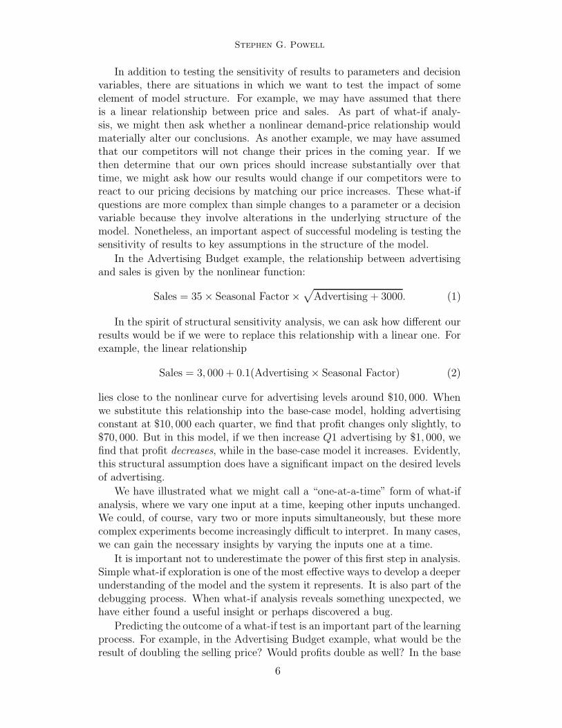
In addition to testing the sensitivity of results to parameters and decisionvariables, there are situations in which we want to test the impact of someelement of model structure. For example, we may have assumed that thereis a linear relationship between price and sales. As part of what-if analy-sis, we might then ask whether a nonlinear demand-price relationship wouldmaterially alter our conclusions. As another example, we may have assumedthat our competitors will not change their prices in the coming year. If wethen determine that our own prices should increase substantially over thattime, we might ask how our results would change if our competitors were toreact to our pricing decisions by matching our price increases. These what-ifquestions are more complex than simple changes to a parameter or a decisionvariable because they involve alterations in the underlying structure of themodel. Nonetheless, an important aspect of successful modeling is testing thesensitivity of results to key assumptions in the structure of the model.

In the Advertising Budget example, the relationship between advertisingand sales is given by the nonlinear function:

Sales = 35 × Seasonal Factor ×√

Advertising + 3000. (1)

In the spirit of structural sensitivity analysis, we can ask how different ourresults would be if we were to replace this relationship with a linear one. Forexample, the linear relationship

Sales = 3, 000 + 0.1(Advertising × Seasonal Factor) (2)

lies close to the nonlinear curve for advertising levels around $10, 000. Whenwe substitute this relationship into the base-case model, holding advertisingconstant at $10, 000 each quarter, we find that profit changes only slightly, to$70, 000. But in this model, if we then increase Q1 advertising by $1, 000, wefind that profit decreases, while in the base-case model it increases. Evidently,this structural assumption does have a significant impact on the desired levelsof advertising.

We have illustrated what we might call a “one-at-a-time” form of what-ifanalysis, where we vary one input at a time, keeping other inputs unchanged.We could, of course, vary two or more inputs simultaneously, but these morecomplex experiments become increasingly difficult to interpret. In many cases,we can gain the necessary insights by varying the inputs one at a time.

It is important not to underestimate the power of this first step in analysis.Simple what-if exploration is one of the most effective ways to develop a deeperunderstanding of the model and the system it represents. It is also part of thedebugging process. When what-if analysis reveals something unexpected, wehave either found a useful insight or perhaps discovered a bug.

Predicting the outcome of a what-if test is an important part of the learningprocess. For example, in the Advertising Budget example, what would be theresult of doubling the selling price? Would profits double as well? In the base

6

Stephen G. Powell

case, with a price of $40, profits total $69, 662. If we double the price, we findthat profits increase to $612, 386. Profits increase by much more than a factorof two when prices double. After a little thought, we should see the reasons.For one, costs do not increase in proportion to volume; for another, demandis not influenced by price in this model. Thus, the sensitivity test helps us tounderstand the nature of the cost structure — that it’s not proportional —as well as one limitation of the model — that no link exists between demandand price.

3.2.1 Data Sensitivity

The Data Sensitivity tool automates certain kinds of what-if analysis. Itsimply recalculates the spreadsheet for a series of values of an input cell andtabulates the resulting values of an output cell. This allows the analyst toperform several related what-if tests in one pass rather than entering eachinput value and recording each corresponding output.

The Data Sensitivity tool is one module in the Sensitivity Toolkit, which isan add-in to Excel (available at http://mba.tuck.dartmouth.edu/toolkit).Once the Toolkit is installed, the Sensitivity Toolkit option will appear on thefar right of the menu bar (see Figure 1). Data Sensitivity and the othermodules can be accessed from this menu. (An equivalent tool called DataTable is built into Excel.)

We illustrate the use of the Data Sensitivity tool in the Advertising Budgetmodel by showing how variations in unit cost from a low of $20 to a high of$30 affect profit. (Note: we will not describe the specific steps required to runany of the tools in the Toolkit in this paper: details can be found in [2] or inthe Help Facility in the Toolkit itself).

Figure 2 shows the output generated by the Data Sensitivity tool. Aworksheet has been added to the workbook, and the first two columns onthe sheet contain the table of what-if values. In effect, the what-if test hasbeen repeated for each unit-cost value from $20 to $30 in steps of $1, and theresults have been recorded in the table. In addition, the table is automaticallyconverted to a graph. As the table and graph both show, annual profits dropas the unit cost increases, and the cost-profit relationship is linear. We canalso see that the breakeven value of the unit cost falls between $29 and $30,since profits cross from positive values to negative values somewhere in thisinterval.

Note that the Data Sensitivity tool requires that we provide a single celladdress to reference the input being varied in a one-way table. The tool willwork correctly only if the input has been placed in a single location. Bycontrast, if an input parameter had been embedded in several cells, the toolwould have given incorrect answers when we tried to vary the input. Thus, theuse of single and separate locations for parameters (or for decisions), which isa fundamental principle of spreadsheet engineering, makes it possible to takeadvantage of the tool’s capability.

7

Stephen G. Powell

We can also use the Data Sensitivity tool to analyze the sensitivity of anoutput to two inputs. This option gives rise to a two-way table, in contrast tothe one-way sensitivity table illustrated above. To demonstrate this feature,we can build a table showing how profits are affected by both Q1 advertisingand Q2 advertising. By studying the results in Figure 3, we can make a quickcomparison between the effect of additional spending in Q1 and the effect ofthe same spending in Q2. As we can observe in the table, moving across a rowgenerates more profit than moving the same distance down a column. Thispattern tells us that we can gain more from spending additional dollars in Q2than from the same additional dollars in Q1. This observation suggests that,starting with the base case, we could improve profits by shifting dollars fromQ1 to Q2. We can also note from the table, or from the three-dimensionalchart that automatically accompanies it, that the relationship between profitsand advertising expenditures is not linear. Instead, profits show diminishingreturns to advertising.

3.2.2 Tornado charts

Another useful tool for sensitivity analysis is the tornado chart. In contrastto the information produced by the Data Sensitivity tool, which shows howsensitive an output is to one or perhaps two inputs, a tornado chart shows howsensitive the output is to several different inputs. Consequently, it shows uswhich parameters have a major impact on the results and which have minorimpact.

Tornado charts are created by changing input values one at a time andrecording the variations in the output. The simplest approach is to vary eachinput by a fixed percentage, such as ±10 percent, of its base-case value. Foreach parameter in turn, we increase the base-case value by 10 percent andrecord the output, then decrease the base-case value by 10 percent and recordthe output. Next, we calculate the absolute difference between these twooutcomes and depict the results in the order of these differences.

The Sensitivity Toolkit contains a tool for generating tornado charts. TheTornado Chart tool provides a choice of three options:

• Constant Percentage

• Variable Percentage

• Percentiles

We will illustrate the Constant Percentage case first. The tornado chartappears on a newly inserted worksheet, as shown in Figure 4. The horizontalaxis at the top of the chart shows profits; the bars in the chart show thechanges in profit resulting from ±10 percent changes in each input. Aftercalculating the values (which are recorded in the accompanying table on thesame worksheet), the bars are sorted from largest to smallest for display in thediagram. Thus, the most sensitive inputs appear at the top, with the largesthorizontal spans. The least sensitive inputs appear toward the bottom, with

8

Stephen G. Powell

the smallest horizontal spans. Drawing the chart using horizontal bars, withthe largest span at the top and the smallest at the bottom, suggests theshape of a tornado, hence the name. If some of the information in the chartseems unclear, details can usually be found in the accompanying table, whichis constructed on the same worksheet by the Tornado Chart tool. In ourexample, we can see in the table that price has the biggest impact (a rangeof more than $108, 000), with unit cost next (a range of nearly $80, 000), andthe other inputs far behind in impact on profit.

The standardization achieved by using a common percentage for the changein inputs (10 percent in our example) makes it easy to compare the resultsfrom one input to another, but it may also be misleading. A 10 percent rangemay be realistic for one parameter, while 20 percent is realistic for another,and 5 percent for a third. The critical factor is the size of the forecast errorfor each parameter. If these ranges are significantly different, we should assigndifferent percentages to different inputs. This can be accomplished using theVariable Percentage option in the Tornado Chart tool.

To illustrate the Variable Percentage option in the Advertising Budgetexample, suppose we limit ourselves to seven parameters: price, cost, fourseasonal factors, and overhead rate. Suppose that, based on a detailed as-sessment of the uncertainty in these parameters, we choose to vary price by 5percent, cost by 12 percent, seasonal factors by 8 percent, and overhead rateby 3 percent. The resulting tornado chart is shown in Figure 5. As the resultsshow, cost now has the biggest impact on profits, partly because it has a largerrange of uncertainty than price.

3.3 Breakeven analysis

Many managers and analysts throw up their hands in the face of uncertaintyabout critical parameters. If we ask a manager to directly estimate marketshare for a new product, the reply may be: “I have no idea what market sharewe’ll capture”. A powerful strategy in this situation is to reverse the sense ofthe question and ask not, “What will our market share be?” but rather, “Howhigh does our market share have to get before we turn a profit?” The trick hereis to look for a breakeven, or cutoff, level for a parameter — that is, a targetvalue of the parameter at which some particularly interesting event occurs,such as reaching zero profits or making a 15 percent return on invested assets.Managers who cannot predict market share can often determine whether aparticular breakeven share is likely to occur. This is why breakeven analysisis so powerful.

Even if we have no idea of the market share for the new product, weshould be able to build a model that calculates profit given some assumption

about market share. Once market share takes the role of a parameter in ourmodel, we can use the Data Sensitivity tool to construct a graph of profit asa function of market share. Then, from the graph, we can find the breakeven

9

Stephen G. Powell

market share quite accurately.New capital investments are usually evaluated in terms of their net present

value, but the appropriate discount rate to use is not always obvious. Ratherthan attempting to determine the appropriate discount rate precisely, we cantake the breakeven approach and ask how high would the discount rate haveto be in order for this project to have an NPV of zero? (The answer to thisquestion is generally known as the internal rate of return.) If the answer is28 percent, we can be confident that the project is a good investment. Onthe other hand, if breakeven occurs at 9 percent, we may want to do furtherresearch to establish whether the appropriate discount rate is clearly belowthis level.

Breakeven values for parameters can be determined manually, by repeat-edly changing input values until the output reaches the desired target. Thiscan often be done fairly quickly by an intelligent trial-and-error search in Ex-cel. In the Advertising Budget example, suppose we want to find the breakevencost to the nearest penny. Recall our example earlier, where we noted thatprofit goes to zero between a unit cost of $29 and a unit cost of $30. Byrepeating the search between these two costs in steps of $0.10, we can findthe breakeven cost to the nearest dime. If we repeat the search once more, insteps of $0.01, we will obtain the value at the precision we seek.

However, Excel also provides a specialized tool called Goal Seek (in theTools menu) for performing this type of search. The tool locates the desiredunit cost as $29.36, and the corresponding calculations will be displayed onthe spreadsheet.

Note that the Goal Seek tool searches for a prescribed level in the relationbetween a single output and a single input. Thus, it requires the parameteror decision being varied to reside in a single location, reinforcing one of ourdesign principles.

3.4 Optimization analysis

Another fundamental type of managerial question takes the form of findinga set of decision variables that achieves the best possible value of an output.In fact, we might claim that the fundamental management task is to makechoices that result in optimal outputs. Solver is an important tool for thispurpose. Solver is an add-in for Excel that makes it possible to optimizemodels with multiple decision variables and possibly constraints on the choiceof decision variables. Optimization is a complex subject, and we can onlyprovide a glimpse of its power here by demonstrating a simple application inthe Advertising Budget example.

Suppose we wish to maximize total profits with an advertising budget of$40, 000. We already know that, with equal expenditures in every quarter,annual profits come to $69, 662. The question now is whether we can achievea higher level of annual profits. The answer is that a higher level is, in fact,

10

Stephen G. Powell

attainable. An optimal reallocation of the budget produces annual profitsof $71, 447. The chart in Figure 6 compares the allocation of the budgetin the base case with the optimal allocation. As we can see, the optimalallocation calls for greater expenditures in quarters Q2 and Q4 and for smallerexpenditures in Q1 and Q3.

This is just one illustration of Solver’s power. Among the many questionswe could answer with Solver in the Advertising Budget example are these:

• What would be the impact of a requirement to spend at least $8, 000 eachquarter?

• What would be the marginal impact of increasing the budget?

• What is the optimal budget size?

One way to answer this last question would be to run Solver with increasingbudgets and trace out the impact on profit. We could do this manually, onerun at a time, but it would be more convenient to be able to accomplishthis task in one step. The Sensitivity Toolkit contains a tool called Solver

Sensitivity that does just this: it runs Solver in a loop while varying one(or two) input parameters. Figure 7 shows the results of running Solver foradvertising budgets from $40, 000 to $100, 000 in increments of $5, 000. Thetable shows that profit increases at a decreasing rate as the budget increases,and beyond about $90, 000 there is no discernible impact from additionalbudget. It also shows how the four decision variables (Q1–Q4 advertising)change as the budget changes.

3.5 Simulation and risk analysis

Uncertainty often plays an important role in analyzing a decision, because withuncertainty comes risk. Until now, we have been exploring the relationshipbetween the inputs and outputs of a spreadsheet model as if uncertainty werenot an issue. However, risk is an inherent feature of all managerial decisions,so it is frequently an important aspect of spreadsheet models. In particular,we might want to recognize that some of the inputs are subject to uncertainty.In other words, we might want to associate probability models with some ofthe parameters. When we take that step, it makes sense to look at outputsthe same way — with probability models. The use of probability models inthis context is known as risk analysis.

One tool for risk analysis in spreadsheets is Crystal Ball, an add-in forMonte Carlo simulation (another is @Risk [5]). This tool allows us to gen-erate a probability distribution for any output cell in a spreadsheet, givenprobability assumptions about some of the input cells. Simulation and riskanalysis are complex subjects. Here, we simply illustrate how Crystal Ball canhelp us answer an important question about risk.

In the Advertising Budget example, we return to the base case, with equalexpenditures of $10, 000 on advertising each quarter. Our base-case analysis,

11

Stephen G. Powell

which assumed that all parameters are known exactly, showed an annual profitof $69, 662. However, we might wonder about the distribution of profits ifthere is uncertainty about the unit price and the unit cost. Future pricesdepend on the number of competitors in our market, and future costs dependon the availability of raw materials. Since both level of competition and rawmaterial supply are uncertain, so, too, are the parameters for our price andcost. Suppose we assume that price is normally distributed with a mean of$40 and a standard deviation of $10, and that unit cost is equally likely tofall anywhere between $20 and $30. Given these assumptions, what is theprobability distribution of annual profits? And how likely is it that profitswill be negative?

Figure 8 shows the probability distribution for profits in the form of ahistogram, derived from the assumptions we made about price and cost. Thegraph shows us that the estimated average profit is $69, 721 under our as-sumptions. It also shows that the probability is about 30 percent that we willlose money. This exposure may cause us to reevaluate the desirability of thebase-case plan.

Once again, we often wish to know how sensitive our simulation results areto one or more input parameters. This suggests running Crystal Ball in a loopwhile we vary the inputs, and to do so we have included the appropriate tool,called CB Sensitivity, in the Sensitivity Toolkit. Figure 9 shows the resultsof running Crystal Ball while we vary the budget from $40, 000 to $100, 000 inincrements of $5, 000, keepting advertising spending equal across the quarters.We plot here not only the mean profit, but the maximum and minimum valuesfrom each of the simulations, to give an idea of the range of outcomes likelyat each step.

4 Research Issues

In contrast to software engineering, which has seen decades of development,spreadsheet engineering is in its infancy. Most of the ideas in this paperhave been adapted from software engineering and tested informally in variousinstructional settings. However, there is little laboratory or field researchto support claims that one or another spreadsheet engineering principle iseffective in actual practice.

Spreadsheet engineers are fundamentally different from software engineers.Most of them would not describe themselves as programmers and most are notaware that they are under-trained for the spreadsheet design and analysis tasksthey perform. Few recognize the risks they and their companies run when theyuse chaotic development processes or fail to use the powerful analytic toolsdescribed here.

The research needs are clear, although how best to carry out this kind of re-search is not. We need to know much more than we do about how spreadsheetsare designed and used in industry. We also need to test various interventions,

12

Stephen G. Powell

including training programs and software add-ins, to see which really improvepractice and which do not. We also need to study how corporate standardsfor training and use of spreadsheets influence the culture and performance ofend-users. While spreadsheet programming has little cache in the computerscience profession, it is likely that more computer programs are written bythe millions of spreadsheet end-users than all professional programmers com-bined. The positive impacts of improving this aspect of programming practiceare correspondingly high.

References

[1] Panko, Ray, What We Know About Spreadsheet Errors, Journal of End User

Computing, Special issue on Scaling Up End User Development, Volume 10, No2. Spring 1998, pp. 15-21.

[2] Powell, Stephen G. and Kenneth Baker, The Art of Modeling with Spreadsheets,New York: John Wiley, 2004.

[3] Solver: http://www.solver.com/

[4] Crystal Ball: http://www.decisioneering.com/crystal ball/index.html/

[5] @Risk: http://www.palisade.com/html/risk.asp

13

Stephen G. Powell

Fig. 1. The advertising budget spreadsheet.

14

Stephen G. Powell

Fig. 2. A graph based on the Data Sensitivity.

15

Stephen G. Powell

Fig. 3. Two-way Data Sensitivity: profit as a function of Q1 and Q2 advertising.

16

Stephen G. Powell

Fig. 4. Tornado Chart using the Constant Percentage option.

17

Stephen G. Powell

Fig. 5. Tornado Chart using the Variable Percentage option.

18

Stephen G. Powell

Fig. 6. Comparison of base-case and optimal allocations.

19

Stephen G. Powell

Fig. 7. Results of Solver Sensitivity.

20

Stephen G. Powell

Fig. 8. Distribution of profits from the Advertising Budget example.

21

Stephen G. Powell

Fig. 9. Results of CB Sensitivity.

22

Design, Implementation and Animation ofSpreadsheets in the Lrc System

Joao Saraiva

Department of Computer Science,

University of Minho, Portugal.

e-mail: jas@di.uminho.pt

Abstract

This paper presents techniques for the design, implementation and animation of spreadsheet-

like tools in the attribute grammar formalism. A real spreadsheet is formally specified and

attribute grammar components that define user interfaces, querying languages and anima-

tions are plugged into the specification through higher-order attributes. From such a spec-

ification an incremental implementation is automatically derived and experimental results

are presented.

Key words: Spreadsheets, Attribute Grammars, Incremental Evaluation,

Functional Programming

1 Introduction

Attribute grammars (AG) [17] have proven to be a suitable formalism to the design

and implementation of both domain specific and general purpose languages. In

fact, powerful systems based on the attribute grammar formalism [23,13,2,9,20,18]

have been constructed. These systems automatically produce very efficient/opti-

mised implementations for languages specified via attribute grammars. While, in

the beginning, AG-based systems were used mainly to specify and derive efficient

(batch) compilers for formal languages, nowadays, AG-based systems are power-

ful tools that not only specify compilers, but also structured-based editors [23],

programming environments [18], visual languages [15], complex pretty printing

algorithms [28], program animations [20,25], etc. Furthermore, attribute grammars

are also a suitable setting to express (circular) lazy programs [12,19,24,5], aspect

oriented compilers [6], incremental algorithms [27], the XML technology [3], etc.

The purpose of this paper is three fold: first, to show that spreadsheet-like

tools can be formally and concisely specified in the higher-order attribute gram-

mar (HAG) formalism [30], and that well-known attribute grammar techniques can

be used to reason about such formal specifications. For example, the AG circu-

larity test can be used to statically detect circularities in the specification which

may induce the non-termination of the spreadsheet. In this paper we present the

specification in the attribute grammar formalism of a student spreadsheet, its in-

teractive interface, and the specification of querying language to query the student

database. Second, to show that efficient incremental implementations can be au-

tomatically derived from an attribute grammar. Spreadsheets heavily rely on a in-

cremental computation model since they have to provide immediate feedback after

user interaction. To derive incremental implementations from AG (usually called

attribute evaluators) we use the Lrc system: a purely functional attribute grammar-

based system [18]. In Lrc efficient incremental evaluation is obtained via function

memoisation. And, finally, to show that the visualisation and animation of the (in-

cremental) execution of the spreadsheet can be obtained from the AG specification.

Such animations provide a visual debugger which allows the user, for example, to

easily understand how the incremental evaluation is performed.

This paper is organised as follows: Section 2 briefly describes higher-order at-

tribute grammars and the Lrc system. Section 3 models a spreadsheet within the

AG formalism. AG components for defining an interactive interface, a query lan-

guage and a visualisation and animation are presented. Section 4 discusses the

incremental implementations derived by the Lrc system from attribute grammar

sprecifications and presents the results of the incremental behaviour of the spread-

sheet. Section 5 presents the conclusions.

2 The Lrc Attribute Grammar based System

The techniques presented in this paper are based on the higher-order attribute

grammar formalism [29]. Higher-order attribute grammars are an important exten-

sion to the attribute grammar formalism. Conventional attribute grammars are aug-

mented with higher-order attributes, the so-called attributable attributes. Higher-

order attributes are attributes whose value is a tree. We may associate, once again,

attributes with such a tree. Attributes of these so-called higher-order trees, may be

higher-order attributes again.

The Lrc system accepts as input a higher-order attribute grammar and generates

purely functional implementations, the so-called attribute evaluators. Lrc generates

both strict, multiple traversal attribute evaluators ( , , and OCaml based

attribute evaluators) and lazy attribute evaluators (expressed as circular lazy pro-

grams in ). Efficient incremental attribute evaluation is obtained via func-

tion memoization. The Lrc system not only produces batch tools (e.g., compilers),

but also programming environments. Such environments have a modern graphical

user interface.

The higher-oder attribute grammar formalism and the Lrc system will be ex-

plained in detail in the next section where we present the HAG to specify a spread-

sheet-like tool.

2

3 The Students Spreadsheet Attribute Grammar

Suppose that we have a (textual) database of students registered in one course.

Each student (i.e., register) has several attributes such as: identification number,

name, and a list of marks (pairs containing the mark identification, and the value

the student got). A possible (concrete) instance of the database is presented below.

1,"Ana",tm=16,p1=15,p2=172,"Eduardo",tm=12,p1=13,p2=153,"David",tm=16,p1=15,p2=17

The first register expresses that the student with number 1, named Ana got the

mark as theoretical mark (tm), in the first project (p1) and in the second

one (p2). This database/language is defined by the following context-free grammar.

A production is denoted as = , where the name of the production,

i.e., , also indicates the term constructor function . The type of the constructor

function is and we say that function takes as argu-

ments values of type and returns a value of type . Roughly speaking,

non-terminal symbols correspond to tree type constructors, and productions corre-

spond to value constructors. We focus on the abstract structure of the language and

we ignore its syntactic sugar, e.g., punctuation symbols, etc.

Students Stud Students

Stud Int String [Mark]

Mark String Real

Fragment 1: The abstract grammar for the students database.

We represent lists of non-terminals by using both the usual functional notation

and explicit constructors.

Having a database with the information about the students marks, the natural

operations we would like to perform on that database are the mapping of a given

formula through all the students in order to calculate, for example, their final clas-

sification. That is to say that we wish to construct a spreadsheet-like tool. To

express a formula we consider a domain specific language (DSL) very much like

the desk calculator language presented in [22]. A concrete example of a formula is

as follows:

FinalMark = (tm + pm)/2where pm = (p1 + p2)/2

To define the formula that is applied to each student we have two possibilities:

We may use a straightforward AG approach where the formula is defined as a

semantic function, written in the declarative language used to express semantic

functions in the AG formalism. As a result, this semantic function will not be

analysed (to infer termination properties) nor optimised by AG techniques. In

3

this approach, the semantic function is part of the AG specification of the tool.

As a result, the formula is processed statically and not dynamically. Thus, if

we wish to use a different formula, the AG has to be modified, analysed and

compiled in order to produced the desired tool.

Or, we may use a key characteristic of higher-order attribute grammars: within

higher-order attribute grammars (HAG) every inductive computation can be mod-

eled through attribution rules. More specifically, inductive semantic functions

can be replaced by higher-order attributes. Thus, we can model the formula,

or, more precisely, that language of formulas as a higher-order attribute of our

spreadsheet. That is, we extend our context-free grammar with new symbols and

productions to define the language of formulas. Then, we associate inerited and

synthesised attributes to its symbols to move context information to the formula

sub-expressions and to synthesise the result of the formula.

In the context of the specification of the student spreadsheet, this is done as

follows: first we define a grammar describing the (abstract) structure of the lan-

guage of formulas and we extend it with attributes and equations. We introduce

an inherited attribute to pass the list of marks as the “argument” of the formula,

and a synthesised attribute to deliver the result of “applying” the formula to its

inherited/argument. After that we have to “apply” such “function” in the context

of every student. To do this, we just introduce a higher-order attribute to repre-

sent the abstract formula, we instantiate its inherited attribute (with the marks of

a particular student) and we use its synthesised result. So, we define a DSL for

formulas as a sub-language of our spreadsheet. Note that in this case the formula

is processed dynamically since it is part of the input sentence. As a result, if the

spreadsheet user wishes to change the formula, he just changes the part of the

input sentence where the formula is defined.

Next we discuss in detail how this latter approach can be implemented in the Lrc

system. The structure of the spreadsheet is defined through the following grammar,

where non-terminal Students is defined in Fragment 1, and non-terminal Formula

represents the (abstract structure) of the formula under consideration.

SpreadSheet Formula Students

Formula Exp Decls

Fragment 2: The abstract grammar for the Spreadsheet-like language.

Let us assume that we have an off-the-shelf AG component whose root non-

terminal is Formula. This non-terminal has one inherited attribute (representing a

finite function mapping variable names to values) and it synthesises one attribute

with the value expressed by the formula. Synthesised (inherited) attributes are pre-

fixed with the up (down) arrow ( ).

Formula

We omit here the attribute declaration and equations of the (trivial) definition

4

of this component. We shall consider that this AG component is included in our

specification in order to create a monolithic AG, which is then analysed and the

respective implementation derived.

In order to map the formula through the database of students, we have to move

the (abstract) formula to the context of every student. Thus, we use one charac-

teristic of the HAG, the so-called syntactic references, meaning that the abstract

tree can be used directly as a value within a semantic equation. In our example the

“syntactic” symbol Formula is used within an equation as follows:

Formula Students

Students form Formula

Fragment 3: Passing the formula to the students.

Instead of defining attributes and equations to move the (abstract) formula down-

wards in the tree (i.e., the student list) via trivial copy rules, we use a special no-

tation to access a remote attribute (up in the tree). The expression Students form

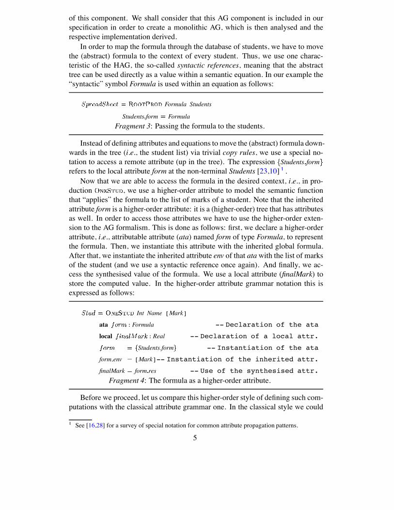
refers to the local attribute form at the non-terminal Students [23,10] .

Now that we are able to access the formula in the desired context, i.e., in pro-

duction , we use a higher-order attribute to model the semantic function

that “applies” the formula to the list of marks of a student. Note that the inherited

attribute form is a higher-order attribute: it is a (higher-order) tree that has attributes

as well. In order to access those attributes we have to use the higher-order exten-

sion to the AG formalism. This is done as follows: first, we declare a higher-order

attribute, i.e., attributable attribute (ata) named form of type Formula, to represent

the formula. Then, we instantiate this attribute with the inherited global formula.

After that, we instantiate the inherited attribute env of that atawith the list of marks

of the student (and we use a syntactic reference once again). And finally, we ac-

cess the synthesised value of the formula. We use a local attribute (finalMark) to

store the computed value. In the higher-order attribute grammar notation this is

expressed as follows:

Int Name [Mark]

ata Formula -- Declaration of the ata

local Real -- Declaration of a local attr.

Students form -- Instantiation of the ata

form env [Mark]-- Instantiation of the inherited attr.

finalMark form res -- Use of the synthesised attr.

Fragment 4: The formula as a higher-order attribute.

Before we proceed, let us compare this higher-order style of defining such com-

putations with the classical attribute grammar one. In the classical style we could

See [16,28] for a survey of special notation for common attribute propagation patterns.

5

express this inductive computation by defining a semantic function that accepts as

arguments the abstract representation of the formula and the list of marks of the

students. It delivers the result of applying the formula to the list of marks. We can

write it as follows:

Int Name [Mark]

finalMark evalFormula Students form [Mark]

Fragment 5: The formula as a semantic function.

where evalFormula is the inductive function. This function has to be defined and in-

cluded in the AG specification. If this semantic function is semantically equivalent

to the formula AG component, then, the previous two AG fragment are semantically

equivalent as well. Furthermore, this approach also supports the dynamic update

of the formula, since its representation is an argument of the semantic function.

But, there are two important differences between these two approaches: while in

the higher-order one, the AG techniques analyse the attribute dependencies, check

for termination properties and, if no circularities are induced, finally, produce an

optimised implementation. In the classical attribute grammar approach, the func-

tion is simply translated to the output without any analysis nor optimisation. Thus,

it can cause the non-termination of the attribute evaluator, and consequently the

non-termination of the spreadsheet!

Spreadsheets are usually displayed in a table-like representation. In [28] we

have presented a generic, off-the-shelf pretty-printing AG component that can be

plugged into our students spreadsheet so as to obtain the desired representation .

This AG component is based on a processor for HTML style tables. It computes

a pretty-printed textual table from a HTML (table) text. More recently we have

extended our original AG in order to synthesise a LATEX, a XML, a VRML, and

HTML table representation. Thus, we have a representation for our abstract tables

in all these concrete languages. Figure 1 displays the ascii representation of a pretty

printed table.

3.1 The Specification of the Spreadsheet Programming Environment

As it was previously stated, types can be defined within the attribute grammar for-

malism via non-terminal symbols. So, we may use this approach to introduce a type

that defines an abstract representation of the interface of spreadsheet-like tools (or

more generally, language-based tools). In other words, we use an abstract context-

free grammar to define an abstract interface. The productions (or constructors) of

such a grammar represent “standard” graphical user interface objects, like menus,

buttons, list boxes, pull donw menus, etc. Next, we present the so-called Lrc ab-

stract interface grammar.

Actually, attribute grammar systems provide a special domain specific language (or, in other

words, a fixed number of combinators) to pretty-print the syntax tree (usually called unparsing

rules).

6

Visuals Toplevel

Toplevel Frame String String

Frame String

Entrylist

String MenuList

String

Ptr

[Frame]

[Frame]

Fragment 6: The Lrc abstract interface grammar.

The non-terminal Visual defines the type of the abstract interface of the tool:

it is a list of objects, that may be displayed in different windows. A

construct displays a frame in a window. It has three arguments: the

frame, a name (for future references) and the window title. The productions applied

to non-terminal Frame define concrete visual objects. For example, production

represents a push-button, represents a list box, etc.

The production represents a visual object that provides structured text

editing [23]. It displays a pretty-printed version of its (tree) argument and allows the

user to interact with it. Such beautified textual representation of the abstract syntax

tree is produced according to the unparse rules specified in the grammar. It also al-

lows the user to point to the textual representation to edit it (via the keyboard), or to

transform it using user defined transformations. The productions and

define combinators: they vertically and horizontally (respectively) combine visual

objects into more complicated ones. These non-terminals and productions can be

directly used in the attribute grammar to define the interface of the environments.

Thus, the interface of the spreadsheets is specified through attribution, i.e., within

the AG formalism.

To define a concrete interface, we need, as we have said above, to define the

mapping from the abstract interface representation into a concrete one. Instead

of defining a concrete interface from scratch, we synthesise a concrete interface

for a existing GUI toolkit, e.g., the TCL/TK GUI toolkit [21]. Indeed, this GUI

component synthesises TCL/TK code defining the interface in the attribute named

tk.

Next, we present an attribute grammar fragment that glues the spreadsheet HAG

with this graphical user interface attribute grammar component. It defines an in-

teractive interface consisting of two visual objects that are vertically combined,

namely: a push-button and the unparsing of the input under consideration. The

root symbol Spreadsheet synthesises the TCL/TK concrete code in the attribute oc-

currence concreteInterface.

7

concreteInterface

Formula Students

ata absInterface Visuals

absInterface let "XML"

[ , ]

in [ "edit" "Students Editor" ]

concreteInterface absInterface tk

Fragment 7: The Spreadsheet graphical user interface.

Figure 1 displays a snapshot of the students spreadsheet produced by Lrc from

a AG specified using the techniques presented in this paper. In the background,

a frame contains a syntax-editor to edit the pretty-printed formula (actually, we

use a list of formulas) and the student database. In this syntax-editor, the user

can point to a formula and dynamically change it. The user can also point to a

particular student and select it through a mouse button. Then, the information of

the student is displayed in a new window, where it can be easily updated. All of

these actions are modelled as (abstract syntax) tree transformations, since the Lrc

system maintains an abstract syntax tree to represent the input under consideration.

Indeed, the (pretty printed) text displayed in the environments, corresponds to the

textual view of such a tree. The Lrc system uses incremental attribute evaluation,

in order to provide immediate real-time feedback, after a user action. This will be

discussed in Section 4.

3.2 Querying the Spreadsheet Through Attribute Grammars

Having specified the students database, the formula to compute their final marks

and how such formula is applied to each of the students, we may wish to compute

which students got good or bad results. Or, we may wish to compute the students

that have a final mark greater than a given number. In other words, we would like

to have some mechanism to be able to query our database.

Rather than defining a particular query language for our student database, we

want to define a generic query language that can not only be used for querying this

particular example, but also to query any other textual database defined within the

AG formalism. That is to say that we want to define a domain specific language

that can be easily embedded in any AG specification. In order to not introduce

yet-another querying language, we will consider the XQuery language: a typed,

functional language for querying Xml, currently being designed by the Xml Query

Working Group of the World-WideWeb Consortium [7,31]. We choose XQuery for

two reasons: first, because attribute grammars and Xml technology are closely re-

lated [4] (both extend the context-free grammar formalism), thus XQuery is indeed

8

Fig. 1. The spreadsheet programming environment produced by the Lrc system from the

students spreadsheet higher-order attribute grammar.

a suitable declarative language to express queries on AG-based language specifi-

cations. Second, an Xml combinator library to map abstract grammars (or trees)

into Xml documents (or Xml trees) is already defined (via attribute grammars) in

Lrc. Thus, we may re-use such a library, firstly to map the abstract grammar of

the language under consideration to an Xml document, and then to query that Xml

document.

Before we briefly explain the XQuery language, let us present a fragment of the

abstract grammar defining the structure of an Xml document.

Document Prolog Miscs Element

Element Name [Attribute] [Content]

Content Element

CharData

Fragment 8: The abstract grammar defining Xml documents.

XQuery uses path expressions that is a mechanism very much like the Unix

notation to define paths on its file system. Instead of using the directory names,

however, it uses the tags contained in an Xml document to indicate the path. Such

tags correspond to the production names (or constructors) of the attribute grammar.

To introduce XQuery, let us consider some example queries on our student

database. To list the students registered in the course we have to write the following

9

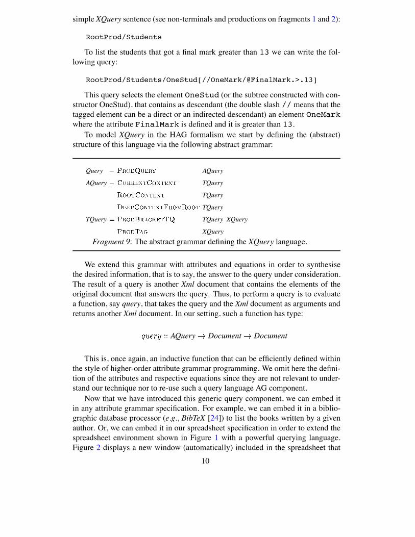
simple XQuery sentence (see non-terminals and productions on fragments 1 and 2):

RootProd/Students

To list the students that got a final mark greater than 13 we can write the fol-lowing query:

RootProd/Students/OneStud[//OneMark/@FinalMark.>.13]

This query selects the element OneStud (or the subtree constructed with con-structor OneStud), that contains as descendant (the double slash // means that thetagged element can be a direct or an indirected descendant) an element OneMarkwhere the attribute FinalMark is defined and it is greater than 13.

To model XQuery in the HAG formalism we start by defining the (abstract)

structure of this language via the following abstract grammar:

Query AQuery

AQuery TQuery

TQuery

TQuery

TQuery TQuery XQuery

XQuery

Fragment 9: The abstract grammar defining the XQuery language.

We extend this grammar with attributes and equations in order to synthesise

the desired information, that is to say, the answer to the query under consideration.

The result of a query is another Xml document that contains the elements of the

original document that answers the query. Thus, to perform a query is to evaluate

a function, say query, that takes the query and the Xml document as arguments and

returns another Xml document. In our setting, such a function has type:

AQuery Document Document

This is, once again, an inductive function that can be efficiently defined within

the style of higher-order attribute grammar programming. We omit here the defini-

tion of the attributes and respective equations since they are not relevant to under-

stand our technique nor to re-use such a query language AG component.

Now that we have introduced this generic query component, we can embed it

in any attribute grammar specification. For example, we can embed it in a biblio-

graphic database processor (e.g., BibTeX [24]) to list the books written by a given

author. Or, we can embed it in our spreadsheet specification in order to extend the

spreadsheet environment shown in Figure 1 with a powerful querying language.

Figure 2 displays a new window (automatically) included in the spreadsheet that

10

Fig. 2. Querying the students spreadsheet: the top frame displays the beautified query that

is performed on the Xml representation of the database (frame on the left). The answer to

the query is displayed as a Xml document on the right frame..

provides the user with a syntax editor to interactively query the student database.

The query being displayed is the example query discussed above. Obviously, the

user can dynamically modify this query and, in this case, the spreadsheet will in-

crementally compute the answer.

3.3 Visualisation and Animation of Spreadsheets

Attribute grammar-base systems statically schedule the computations, and, auto-

matically generate implementations for the AGs - the so-called attribute evaluators

- based on the dependencies induced by the attribution rules. Such evaluators are

usually implemented as tree-walk evaluators: a function that walks over the ab-

stract tree (representing the input under consideration) while computing attribute

values (this task is usually called tree decoration). Thus, attribute grammars can

be visualised by displaying the abstract tree in a graphical representation, and ani-

mated by displaying the tree decoration process in that tree (for example, by mark-

ing in the graphical representation the tree node being visited and by displaying the

attribute values being computed).

Thus, we introduce a generic component for the visualisation and animation of

AGs. We wish to use this AG as a generic visual and animation AG component. We

start by defining an abstract grammar that is sufficiently generic to define all possi-

ble abstract tree structures we may want to visualise and animate. The grammar is

as follows:

11

TreeViz TreeId TreeStmt

TreeStmt NodeStmt

EdgeStmt

AttrStmt

NodeStmt NodeId Attr

EdgeStmt NodeId EdgeRHS Attrs

EdgeRHS EdgeOp NodeId

Attr AttrId AttrVal

The non-terminals TreeId, NodeId, EdgeOp, AttrId, AttrVal define sequences of

characters (strings). In order to make it easier to use this component, we define a set

of functions/macros that, using the productions of this AG component, define usual

occurring node formats in our trees. Next, we present four functions that define the

shape of a node as a record (attrShapeRecord), as a circle (attrShapeCircle), as the

value of a node label (attrLabel), and, finally, as a node that contains a value and

an arrow to a child node. These functions are presented next.

attrShapeRecord = ”shape” ”record”

attrShapeCircle = ”shape” ”circle”

attrLabel label = ”label” label

nodeRecord1 val father child =

[ ( father) [attrShapeRecord , attrLabel (val ++ "|<c>")]

, ( "c") [ "->" child] ]

The label is a string that defines the format of the node record. The non-terminal

EdgeOpis a string defining the direction of the arrow.

The above grammar defines the abstract structure of abstract trees only. To have

a concrete graphical representation of the trees, however, we need to map such

abstract tree representation into a concrete one. Rather than defining a concrete

interface from scratch and implementing a tree/graph visualization system (and

reinventing the wheel!), we can synthesise a concrete interface for existing high

quality graph visualization systems, e.g., the GraphViz system [8]. We omit here

again attributes and attribution rules that we have associated to the visualization

grammar since they are neither relevant to reuse this component nor to understand

our techniques.

This grammar component is context-free (it does not have any inherited at-

tributes) and synthesises two attributes graphviz and xml, both of type string. These

two attributes synthesise a textual representation of trees in the GraphViz input lan-

guage. The first attribute displays trees in the usual graphic tree representation,

while the second one uses a Xml tree-like representation (where the production

names are the element tags).

12

TreeViz

We are now in position to “glue” this component to the spreadsheet AG. Let us

start by defining the attribute and the equations that specify the construction of the

GraphViz representation.

[ ]

viztree nodeEmptyCircle Students

Stud Students

viztree nodeRecord2 treeRef treeRef

treeRef ++ viztree ++ viztree

[ ]

Int String [Mark]

viztree nodeRecord1 ++ int2str Int treeRef [Marks]

Fragment 10: Constructing the Visual Tree.

Where the function treeRef returns a unique identifier of its tree-value argu-

ment (the tree pointer). Next, we declare a higher-order attribute, i.e., attributable

attribute (ata) named visualTree, in the context of the single production applied to

the root non-terminal of the spreadsheet AG. The HAG fragment looks has follows:

Formula Students

ata TreeViz

viztree

++ viztree

visualTree graphviz

Figure 3 shows two different snapshots (displayed by GraphViz) of the tree that

is obtained as the result of running the spreadsheet with the example sentence. As

we can see the tree is displayed as a Direct Acyclic Graphs. This happens because

we are using the incremental model of attribute evaluation of Lrc. We will return to

this subject in the next section.

Besides computing the graphical representation of the tree, the processor gen-

erated by Lrc also produces a sequence of node transitions. This is exactly the

sequence of visits the evaluator performs to decorate the tree under consideration.

Such sequence can be loaded in and animated in GraphViz, either in single step or

in continuous mode, forwards and backwards. Different colors (or different shadow

intensities in a black and white printing) are used to identify the number of times

13

Fig. 3. The DAG representing the example sentence after processing the first student (left)

and after attribute evaluation (right).

the nodes have been visited. Thus, light gray means a single visit, gray (or color

blue) meand two visits and drak gray (or color red) means 3 or more visist.

The snapshot on the left shows the attribute evaluator when processing the first

student. The shadowed nodes are the nodes that have already been visited. The

snapshot on the right shows the tree after attribute evaluation. As we can see,

the (shared) list of marks of students number and has been visited only once

(light gray nodes). Its root, however, has been visited twice (gray node). On its

second visit a cache hit occurred: the formula under consideration has already been

“applied” to that argument.

4 Implementation of Attribute Grammar-based Spreadsheets

A spreadsheet-like system has to react and to provide answers in real-time. Con-

sequently, the delay between the user interaction and the system response is an

extremely important aspect in such interactive systems. Thus, one of the key fea-

tures to handle such interactive environments is the ability to perform efficient re-

computations. That is to say that spreadsheets use an efficient incremental com-

putational model. Implementing from scratch an efficient incremental engine is a

complex task.

We use an efficient incremental computational model that efficiently (and ele-

gantly) handles HAGs: the memoization (and posterior reuse) of calls to the func-

tions of the attribute evaluator. Such functions traverse/visit the tree in order to

assign a meaning to input under consideration. To achieve efficient function mem-

14

oization we use the following combination of techniques:

Purely functional attribute evaluators: Syntax trees are visited and decorated by

strict, purely functional attribute evaluators. The attribute evaluators are based on

the visit-sequence paradigm [14]: The attribute evaluator consists of a set of visit-

functions, each of which perform the computations scheduled (by the attribute

grammars scheduling algorithm) for a particular traversal of the evaluator. The

attribute instances are not stored in the tree nodes, but, instead, they are the

arguments and the results of pure (side-effect free) functions: the visit-functions.

The different traversal functions are “glued” by intermediate data structures: the

visit-trees. Such redundant intermediate structures can be eliminated by using

our deforestation techniques for AGs [26].

Data constructor memoization: Since attribute instances are not stored in the

syntax tree, multiple instances of the syntax tree can be shared. That is, trees

are collapsed into minimal Direct Acyclic Graphs (DAG) (Figure 3 displays

the DAG constructed for the example input). DAGs are obtained by construct-

ing trees bottom-up and by using constructor function memoization to elimi-

nate replication of common sub-expressions. This technique, also called hash-

consing [11,1], guarantees that two identical objects share the same records on

the heap, and thus are represented by the same pointer.

Data constructor memoization considerably reduces the memory usage, al-

lows for efficient equality tests between all terms because a pointer comparison

suffices and, as we will explain next, makes efficient visit-function memoization

possible.

Visit-function memoization: Due to the pure nature of the visit-functions, incre-

mental evaluation is obtained by memoizing calls to the evaluator’s strict visit-

functions. Memoization is obtained by storing in a function cache calls to visit-

functions. Every call corresponds to a entry, in the function cache, that records

both the arguments and the results of one call to a visit-function.

The essence of the visit-function memoization is as follows: each time a mem-

oized visit-function is applied to a subtree and to a set of remaining arguments

(i.e., values of attribute instances), we search a cache to check whether that func-

tion was previously applied to those arguments, or not. If the cache contains an

entry corresponding to the call, the result in that entry is returned. If no such en-

try exists, the visit-function is applied to the arguments and the call is memoized.

In the animations produced by Lrc the reuse of a function call can be easily

identified since when visiting a node the animation skip the visits to the children

of that node. In our running example this occured in the second visit to the root

of the shared list of marks.

4.1 Benchmarking the Spreadsheet

Next, we present results obtained when executing the spreadsheet with a real stu-

dent database: the database contains the students, and all their marks, who follow

the compiler construction course where this tool was proposed as the course project.

15

The number of students attending this course was and to each of them corre-

sponds evaluation elements (i.e., partial evaluation marks) which are used by a

list of formulas to compute different aspects of their evaluation (for example, a

particular exam, the projects mark, the final mark, etc). This database was con-

structed and is maintained by the spreadsheet tool. Actually, we have used this

tool to manage the course, as opposed to the use of a commercial tool. The table

below presents results obtained both with non-incremental evaluation, i.e., without

memoization of the calls to the evaluator functions, and with incremental evalua-

tion, i.e., with memoization of the function calls. It shows the number of functions

evaluated (cache misses), functions reused (cache hits), and time (in seconds on

an 2.4 GHz Intel Pentium processor, running Linux Red-Hat 9). We consider six

different situations: the processing of the database from scratch (i.e., starting with

an empty function cache), the editing of the database (i.e., the reaction after adding

a new formula, editing one, and editing a student mark), and the querying of the

database (i.e., performing a query to select a student and performing the example

query).

Non-Incremental Incremental

cache cache time cache cache time

misses hits secs misses hits secs

Scratch 408568 - 7.8 41730 37052 1.65

Editing:

Add a formula 435212 - 11.3 18356 34317 1.30

Edit a formula 408568 - 10.4 8148 11409 0.45

Edit a stud. mark 408568 - 10.4 3393 3016 0.23

Querying:

Select a student 501208 - 12.5 22158 47412 1.63

Example query 623000 - 13.3 27871 59307 1.73

As the above table shows, our incremental model of attribute evaluation pro-

duces efficient implementations. Even when processing an input from scratch, the

incremental evaluator computes of the functions as compared to when no in-

crementally is used ( functions evaluated against , respectively) and is

almost times faster. The reused functions are, in this case, due to the decoration of

the same tree (representing the formula) with the same inherited attributes (the same

marks). Or, in other words, the reuse of previous evaluations of the formula with

the same “arguments”. As expected, the tool handles very well updates of the input:

adding a new (global) formula requires the re-evaluation of of the functions

computed with non-incremental evaluation and of the functions if we consider

incremental evaluation. Better results are obtained with local changes (e.g., editing

16

a student mark). A query in this spreadsheet performs like a global change since

the results of applying formulas are being considered by the query. Nevertheless,

using the incremental model is times faster than the non-incremental one.

5 Conclusions

A spreadsheet was efficiently and elegantly specified within the style of attribute

grammar programming. The Lrc system processed such a specification and derived

a correct and efficient implementation. The results of incremental evaluation show

that spreadsheets are a natural context for incremental evaluation. Actually, these

results are much better than previous results of incremental evaluation (mainly pro-

duced in the context of syntax-based editing).

References

[1] A. W. Appel and M. J. R. Goncalves. Hash-consing Garbage Collection. Technical

Report CS-TR-412-93, Princeton University, Dept. of Computer Science, Feb. 1993.

[2] L. Augusteijn. The elegant compiler generation system. In P. Deransart and

M. Jourdan, editors, Attribute Grammars and their Applications (WAGA), volume 461

of Lecture Notes in Computer Science, pages 238–254. Springer-Verlag, New York–

Heidelberg–Berlin, Sept. 1990. Paris.

[3] H. Boley. Attribute grammars and xml. In Workshop on Attribute Grammars, XML,

and RDF. University of St. Gallen, Sept. 2000.

[4] N. Bradley. The XML Companion. Addison Wesley, 1998.

[5] O. de Moor, K. Backhouse, and D. Swierstra. First-Class Attribute Grammars. In

D. Parigot and M. Mernik, editors, Third Workshop on Attribute Grammars and their

Applications, WAGA’00, pages 1–20, Ponte de Lima, Portugal, July 2000. INRIA

Rocquencourt.

[6] O. de Moor, S. Peyton-Jones, and E. van Wyk. Aspect-Oriented Compilers. In

Proceedings of the First International Symposium on Generative and Component-

Based Software Engineering (GCSE ’99), volume 1799 of LNCS. Springer-Verlag,

Sept. 1999.

[7] W. W. Draft. XQuery 1.0: An XML Query Language, April 2002.

[8] E. R. Gransner and S. C. North. An open graph visualization system and its

applications to software engineering. Software Practice and Experience, 00(S1):1–

29, 1999.

[9] R.W. Gray, V. P. Heuring, S. P. Levi, A.M. Sloane, and W.M.Waite. Eli: A Complete,

Flexible Compiler Construction System. Communications of the ACM,, 35(2):121–

131, February 1992.

[10] G. Hedin. Reference Attributed Grammars. In D. Parigot and M. Mernik, editors,

Second Workshop on Attribute Grammars and their Applications, WAGA’99, pages

153–172, Amsterdam, The Netherlands, Mar. 1999. INRIA rocquencourt.

[11] J. Hughes. Lazy memo-functions. In J.-P. Jouannaud, editor, Functional

Programming Languages and Computer Architecture, volume 201 of LNCS, pages

129–146. Springer-Verlag, September 1985.

17

[12] T. Johnsson. Attribute grammars as a functional programming paradigm. In G. Kahn,

editor, Functional Programming Languages and Computer Architecture, volume 274

of LNCS, pages 154–173. Springer-Verlag, September 1987.

[13] M. Jourdan, D. Parigot, C. Julie, O. Durin, and C. Le Bellec. Design, implementation

and evaluation of the FNC-2 attribute grammar system. In ACM SIGPLAN’90

Conference on Programming Languages Design and Implementation, volume 25,

pages 209–222. ACM, June 1990.

[14] U. Kastens. Ordered attribute grammars. Acta Informatica, 13:229–256, 1980.

[15] U. Kastens and C. Schmidt. Vl-eli: A generator for visual languages. In M. van den

Brand and R. Laemmel, editors, Electronic Notes in Theoretical Computer Science,

volume 65. Elsevier Science Publishers, 2002.

[16] U. Kastens and W. Waite. Modularity and reusability in attribute grammars. Acta

Informatica, 31:601–627, June 1994.

[17] D. E. Knuth. Semantics of Context-free Languages. Mathematical Systems Theory,

2(2):127–145, June 1968. Correction: Mathematical Systems Theory 5, 1, pp. 95-96

(March 1971).

[18] M. Kuiper and J. Saraiva. Lrc - A Generator for Incremental Language-Oriented

Tools. In K. Koskimies, editor, 7th International Conference on Compiler

Construction, CC/ETAPS’98, volume 1383 of LNCS, pages 298–301. Springer-Verlag,

April 1998.

[19] M. Kuiper and D. Swierstra. Using attribute grammars to derive efficient functional

programs. In Computing Science in the Netherlands CSN’87, November 1987.

[20] M. Mernik, M. Lenic, E. Avdicausevic, and V. Zumer. Lisa: An interactive

environment for programming language development. In N. Horspool, editor,

International Conference on Compiler Construction, CC/ETAPS’02, volume 2304 of

LNCS, pages 1–4. Springer-Verlag, April 2002.

[21] J. Ousterhout. Tcl and the Tk toolkit. Addison Wesley, 1994.

[22] J. Paakki. Attribute Grammar Paradigms - A High-Level Methodology in Language

Implementation. ACM Computing Surveys, 27(2):196–255, June 1995.

[23] T. Reps and T. Teitelbaum. The Synthesizer Generator. Springer, 1989.

[24] J. Saraiva. Purely Functional Implementation of Attribute Grammars. PhD thesis,

Department of Computer Science, Utrecht University, The Netherlands, December

1999. ftp://ftp.cs.uu.nl/pub/RUU/CS/phdtheses/Saraiva/.[25] J. Saraiva. Component-based Programming for Higher-Order Attribute Grammars.

In D. Batory, C. Consel, and W. Taha, editors, Proceedings of the ACM

SIGPLAN/SIGSOFT Conference on Generative Programming and Component

Engineering, GPCE 2002, Held as Part of the Confederation of Conferences on

Principles, Logics, and Implementations of High-Level Programming Languages, PLI

2002, Pittsburgh, PA, USA, October 3-8, 2002, volume 2487 of LNCS, pages 268–282.

Springer-Verlag, October 2002.

[26] J. Saraiva and D. Swierstra. Data Structure Free Compilation. In Stefan Jahnichen,

editor, 8th International Conference on Compiler Construction, CC/ETAPS’99,

volume 1575 of LNCS, pages 1–16. Springer-Verlag, Mar. 1999.

[27] J. Saraiva, D. Swierstra, and M. Kuiper. Functional Incremental Attribute Evaluation.

In David Watt, editor, 9th International Conference on Compiler Construction,

CC/ETAPS2000, volume 1781 of LNCS, pages 279–294. Springer-Verlag, Mar. 2000.

[28] D. Swierstra, P. Azero, and J. Saraiva. Designing and Implementing Combinator

Languages. In D. Swierstra, P. Henriques, and J. Oliveira, editors, Third Summer

18

School on Advanced Functional Programming, volume 1608 of LNCS, pages 150–

206. Springer-Verlag, Sept. 1999.

[29] H. Vogt, D. Swierstra, and M. Kuiper. Higher order attribute grammars. In ACM

SIGPLAN ’89 Conference on Programming Language Design and Implementation,

volume 24, pages 131–145. ACM, July 1989.

[30] H. Vogt, D. Swierstra, and M. Kuiper. Efficient incremental evaluation of higher

order attribute grammars. In J. Maluszynki and M. Wirsing, editors, Programming

Language Implementation and Logic Programming, volume 528 of LNCS, pages 231–

242. Springer-Verlag, 1991.

[31] P. Wadler. Xquery: a typed functional language for querying XML. In Fourth Summer

School on Advanced Functional Programming, Oxford, August 2002.

19

FOS 2004

Dealing with life in the cells:An experimental study

David Wakeling 1

Bioinformatics Group, University of Exeter, Exeter, United Kingdom

Abstract

Cell biologists have access to the “parts list” data for the cells of many organisms,but limited understanding of how these parts go together to make a cell “comealive”. A cell simulator could improve this understanding considerably. Our goalis to make cell simulation as convenient as spreadsheet calculation by making thesimulator resemble a spreadsheet. In this paper, we describe our prototype simulatorand report on our early experience with it.

Key words: cell simulation, spreadsheet

1 Introduction

Cell biologists have access to “parts list” data for the cells of many organisms,but limited understanding of how these parts go together to make a cell “comealive”. A cell simulator could improve this understanding considerably, asTomita remarks

To say that we understand the overall behaviour of the cell, we must be ableto answer questions such as: ‘How would the cell behave if we change the en-vironment, for example, by adding or decreasing a certain substance?’ and‘What is the result if a certain gene gets knocked out or over-expressed?’Slightly more sophisticated questions include ‘What gene needs to be in-serted for the cell to behave in such a way?’ and ‘What is the ideal culturemedium in which to maximize the cell’s ability to do such a thing?’ [10].

Our goal is to make cell simulation as convenient as spreadsheet calculationby making the simulator resemble a spreadsheet. In this paper, we describeour prototype simulator and report on our early experience with it. The paperis organised as follows. Section 2 provides a brief reminder of how ordinarydifferential equations are solved numerically. Section 3 describes our simulator.Section 4 gives its evaluation and typing rules. Section 5 presents an example

1 Email: D.Wakeling@exeter.ac.uk

Wakeling

model. Section 6 shows how this model can be simulated with our simulator.Section 7 shows how it can be simulated with the E-Cell simulator. Section 8reports the results of a small an experimental study. Section 9 considers someclosely related and possible future work. Section 10 concludes.

2 Solving ordinary differential equations numerically

An ordinary differential equation takes the form dx/dt = f(t, x), and describeshow the dependent variable, x, representing some value of interest changes withthe independent variable, t, usually representing time. An initial value problemis one where the value of x = x0 is specified at time t = t0. A simulation mustsolve systems of such equations numerically, and one common way to do so isto use the fourth-order Runge-Kutta method, summarised by the equations

k1 =hf(tn, xn)

k2 =hf(tn +h

2, xn +

k1

2)

k3 =hf(tn +h

2, xn +

k2

2)

k4 =hf(tn + h, xn + k3)

xn+1 =xn +k1

6+

k2

3+

k3

3+

k4

6tn+1 = t + h

where the constant h is the time step size.

3 Our prototype simulator

Our prototype simulator incorporates several ideas.

3.1 A new approach to functions

Recently, Peyton Jones et. al. proposed a new approach to functions inspreadsheets [6]. Functions are entered into a worksheet 2 , with some cellsallocated for the arguments, and another for the result. See figure 1. Here, theworkbook has a worksheet for the function f2c that converts from Fahrenheitto Celsius. By (our) convention, the first few cells in column A of a worksheetthat defines a function are allocated for the argument values, and the onebelow those is allocated for the result formula.

2 Throughout this paper, we use the terminology and features of Microsoft’s popular Excelspreadsheet for our discussion and examples. Other spreadsheets are similar.

2

Wakeling

Fig. 1. A worksheet defining a function.

3.2 A history mechanism

Wray and Fairbairn introduced a history mechanism in their Nas spread-sheet [13]. Here, the value of a cell may depend on its own “last” value, andcalculation takes place when a Tick button is pressed. Thus, a cell might con-tain the value and formula 42 = last + 1 which, after pressing Tick, wouldchange to 43 = last + 1. There must always be a value in a cell with aformula involving last.

3.3 A built-in function for solving ordinary differential equations

Spreadsheets usually provide a number of built-in functions for common math-ematical, statistical and scientific operations. In the same way, a built-in func-tion can be provided for solving ordinary differential equations. To solve anequation of the form dx/dt = f(t, x) with an initial value x = x0 at t = t0, acell might contain the value and formula x0 = ODE(f(t, last), h), where t isa reference to a cell containing the value and formula t0 = last + h, and h isa reference to a cell containing the value of the step size. Each ODE applicationtakes one step towards solving the equation. Again, there must always be avalue in a cell with a formula involving an ODE application, which must alwaysbe outermost.

Most often, a system of ordinary differential equations must be solved, inwhich several equations are defined in terms of one another. In a functionalsetting, each of these equations must be passed the current values of the othersas additional arguments, a1, . . . , an. A definition of ODE using the Runge-Kuttamethod is as follows

ODE(f(t, a1, . . . , an, x), h)= x + k1/6 + k2/3 + k3/3 + k4/6

wherek1 = hf(t, a1, . . . , an, x)k2 = hf(t + h/2, a1, . . . , an, x + k1/2)k3 = hf(t + h/2, a1, . . . , an, x + k2/2)k4 = hf(t + h, a1, . . . , an, x + k3)

Of course, other definitions are possible using other methods.

3

Wakeling

4 Evaluation and typing rules

In programming language research, valuable clarity comes from formalisingrules for evaluation and typing, and we do something similar for our prototypesimulator.

4.1 Terms and types

A workbook maps from names to worksheets, and a worksheet from cell ref-erences to cells. A cell is a pair of expressions representing a value and aformula, and an expression is either a label, a number, a cell reference, thehistory variable, or the application of a name to an argument. See figure 2.In reality, of course, it is essential to allow the basic mathematical operators,

w ::= {gi ⇒ si}ni=1 — workbooks

s ::= 〈ri ⇒ ci〉mi=1 — worksheets

c ::= (e1, e2) — cells

e ::= l | n | r | last | g (e) — expressions

Fig. 2. The syntax of terms.

parentheses for grouping, built-in functions, and application of a worksheetto more than one argument. These extensions present no difficulty, and areomitted here only to save space.

A type is either a label, number or function type. See figure 3.

T ::= Label | Number | (Number) → Number

Fig. 3. The syntax of types.

4.2 Evaluation rules

An evaluation judgement takes the form s : t ⇓ s′ : t′, and says that evaluatinga term t in a state s yields a term t′ in a state s′. A state may be made up of amapping Γ from names to worksheets, a mapping ∆ from cell references to cellsand a value φ to be used for the history variable. To the left of “⇓”, M [a &→ b]indicates extension of a mapping, and M [. . . , a &→ b, . . .] reveals some part ofit. To the right of “⇓”, such details are omitted, since any changes can easilybe inferred from elsewhere.

Evaluation judgements can be used to write evaluation rules for terms.The rule E-Book says that evaluating a workbook involves evaluating onlythe visible worksheet (this is the one being “ticked”). See figure 4. The ruleE-Sheet says that evaluating a worksheet involves evaluating all of its cells(this must be done in natural order). See figure 5. There are two evaluation

4

Wakeling

E-BookΓ[gi &→ si]ni=1 : s√ ⇓ Γ′ : s′√

Γ : {. . . , g√ ⇒ s√, . . .}ni=1 ⇓ Γ′ : {. . . , g√ ⇒ s′√, . . .}n

i=1

Fig. 4. The evaluation rule for workbooks.

E-SheetΓ; ∆[ri &→ ci]mi=1 : ci ⇓ Γ′; ∆′ : c′iΓ : 〈ri ⇒ ci〉mi=1 ⇓ Γ′ : 〈ri ⇒ c′i〉mi=1

, ri in natural order

Fig. 5. The evaluation rule for worksheets.

rules for cells. See figure 6. The rules E-Cell1 and E-Cell2 say that evaluating

E-Cell1Γ; ∆ : (v, ?) ⇓ Γ; ∆ : (v, ?)

E-Cell2Γ; ∆; v : f ⇓ Γ′; ∆′ : e

Γ; ∆ : (v, f) ⇓ Γ′; ∆′ : (e, f)

Fig. 6. The evaluation rules for cells.

a cell is trivial if it has a value, but no formula; otherwise, the formula mustbe evaluated to give the value. There are five evaluation rules for expressions.See figure 7. The rules E-Lab and E-Num say that evaluating constants is

E-LabΓ; ∆; φ : l ⇓ Γ; ∆ : l

E-NumΓ; ∆; φ : n ⇓ Γ; ∆ : n

E-RefΓ; ∆[. . . , r &→ (v, f), . . .]; φ : r ⇓ Γ; ∆ : v

E-HistΓ; ∆; φ : last ⇓ Γ; ∆ : φ

E-App

Γ; ∆; φ : x ⇓ Γ′; ∆′ : y

Γ′[. . . , g &→ s, . . .]; s[A1 &→ (y, ?)]; φ : A2 ⇓ Γ′′; s′′ : e

Γ; ∆; φ : g(x) ⇓ Γ′′; ∆′′ : e

Fig. 7. The evaluation rules for expressions.

trivial. The rule E-Ref says that a cell reference evaluates to the value of acell that must itself already have been evaluated because evaluation is donein natural order. The rule E-Hist says that last evaluates to the value ofthe cell whose formula caused it to be evaluated. The rule E-App says thatevaluating an application amounts to evaluating the result cell of the functionworksheet when its argument cell contains the argument value.

5

Wakeling

4.3 Typing rules

A typing judgement takes the form A ' t :: T , and says that under theassumptions A, a term t has type T . The assumptions are made up of amapping Λ from names to types, and a mapping Ξ from cell references totypes.

Typing judgements can be used to write typing rules for terms. The rule T-Book says that a workbook has (arbitrarily) the type of the visible worksheet.See figure 8. The rule T-Sheet says that a worksheet has a type formed from

T-BookΛ[. . . , gi :: Ti, . . .] ' s√ :: T√

Λ ' {. . . , g√ ⇒ s√, . . .}ni=1 :: T√

Fig. 8. The typing rule for workbooks.

those of the argument and result cells, which must be Numbers. See figure 9.

T-Sheet

Λ; Ξ[A1 :: Number] ' ci :: Ti

Λ; Ξ[A1 :: Number, ri :: Ti] ' c2 :: Number

Λ ' 〈A1 ⇒ c1, A2 ⇒ c2, ri ⇒ ci〉mi=3 :: (Number) → Number

Fig. 9. The typing rule for worksheets.

There are two typing rules for cells. See figure 10. The rules T-Cell1 and T-

T-Cell1Λ; Ξ ' v :: T

Λ; Ξ ' (v, ?) :: T

T-Cell2Λ; Ξ ' f :: Number

Λ; Ξ ' (v, f) :: Number

Fig. 10. The typing rules for cells.

Cell2 say that a if a cell has value, but no formula, then its type is that of thevalue; otherwise, it is that of the formula, which must be Number. There arefive typing rules for expressions. See figure 11. The rules T-Lab and T-Num

say that constants have the obvious basic types. The rule T-Ref says that acell reference has the type given in the assumptions, and the rule T-Hist saysthat last must have type Number. The rule T-App says that the applicationof a worksheet to an argument of type Number has type Number.

5 An example model

Hodgkin and Huxley modelled the current flow through the surface membraneof the nerve fibre of a squid as the sum of the capacitative, sodium, potassiumand leakage currents [4].

6

Wakeling

T-LabΛ; Ξ ' l :: Label

T-NumΛ; Ξ ' n :: Number

T-RefΛ; Ξ[. . . , r :: T, . . .] ' r :: T

T-HistΛ; Ξ ' last :: Number

T-AppΛ; Ξ ' x :: Number Λ; Ξ ' g :: (Number) → Number

Λ; Ξ ' g(x) :: Number

Fig. 11. The typing rules for expressions.

5.1 The capacitative current

The capacitative current, Icap, is given by

Icap = Cm ×dVm

dt

where Cm is the membrane capacitance, and Vm the transmembrane potential.

5.2 The sodium current

The sodium current, INa, is given by

INa = gNa,max × m3 × h × (Vm − ENa)

where gNa,max is the maximum conductance of sodium, and m and h satisfythe equations

dm

dt= αm × (1 − m) − βm × m

dh

dt= αh × (1 − h) − βh × h

The rate coefficients were found by curve-fitting to be

αm =0.1 × (Vm + 25.0)

exp(0.1 × (Vm + 25.0)) − 1.0

βm =4 × exp(Vm/18.0)

αh =0.07 × exp(Vm/20.0)

βh =0.1

exp(0.1 × (Vm + 30.0)) + 1.0

7

Wakeling

5.3 The potassium current

The potassium current, IK, is given by

IK = gK,max × n4 × (Vm − EK)

where gK,max is the maximum conductance of potassium, and n satisfies theequation

dn

dt= αn × (1 − n) − βn × n

The rate coefficients were again found by curve-fitting to be

αn =0.01 × (Vm + 10.0)

exp(0.1 × (Vm + 10.0)) − 1.0

βn = 0.125 × exp(Vm/80.0)

5.4 The leakage current

The leakage current, IL, is given by

IL = gL × (Vm − EL)

where EL is the reversal potential for the leakage current.

5.5 The total current

Combining the equations, the total current across a cell membrane, I, is givenby

I = Cm ×dVm

dt+ INa + IK + IL

This can be rearranged to

dVm

dt=

I − INa − IK − IL

Cm

6 Simulation with our prototype simulator

In our simulator, the ordinary differential equations of the example model areentered into a workbook. See figure 12. The run worksheet drives the simula-tion. Cells A4 — A7 deal with calculation of the dependent variables Vm, m, hand n, and cells A2 and C1 with calculation of the dependent variable, t. Theremaining cells are used for intermediate calculations, constant values and la-bels. Other worksheets are used in the calculation of the dependent variables.To save space, we have shown only the calc_m worksheet, as calc_h, calc_nand calc_vm are very similar. Simulation is performed by pressing a “recal-culate” button and specifying the number of steps (or “ticks”). Our simulatoris written from scratch in Haskell using the WxHaskell library.

8

Wakeling

The run worksheet.

The calc m worksheet.

Fig. 12. Model entry with our prototype simulator.

9

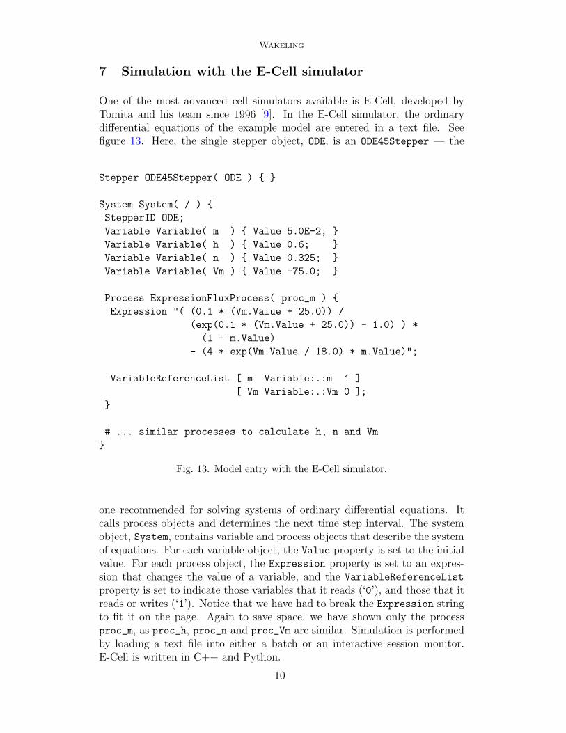
Wakeling

7 Simulation with the E-Cell simulator

One of the most advanced cell simulators available is E-Cell, developed byTomita and his team since 1996 [9]. In the E-Cell simulator, the ordinarydifferential equations of the example model are entered in a text file. Seefigure 13. Here, the single stepper object, ODE, is an ODE45Stepper — the

Stepper ODE45Stepper( ODE ) { }

System System( / ) {StepperID ODE;Variable Variable( m ) { Value 5.0E-2; }Variable Variable( h ) { Value 0.6; }Variable Variable( n ) { Value 0.325; }Variable Variable( Vm ) { Value -75.0; }

Process ExpressionFluxProcess( proc_m ) {Expression "( (0.1 * (Vm.Value + 25.0)) /

(exp(0.1 * (Vm.Value + 25.0)) - 1.0) ) *(1 - m.Value)

- (4 * exp(Vm.Value / 18.0) * m.Value)";

VariableReferenceList [ m Variable:.:m 1 ][ Vm Variable:.:Vm 0 ];

}

# ... similar processes to calculate h, n and Vm}

Fig. 13. Model entry with the E-Cell simulator.

one recommended for solving systems of ordinary differential equations. Itcalls process objects and determines the next time step interval. The systemobject, System, contains variable and process objects that describe the systemof equations. For each variable object, the Value property is set to the initialvalue. For each process object, the Expression property is set to an expres-sion that changes the value of a variable, and the VariableReferenceListproperty is set to indicate those variables that it reads (‘0’), and those that itreads or writes (‘1’). Notice that we have had to break the Expression stringto fit it on the page. Again to save space, we have shown only the processproc_m, as proc_h, proc_n and proc_Vm are similar. Simulation is performedby loading a text file into either a batch or an interactive session monitor.E-Cell is written in C++ and Python.

10

Wakeling

8 An experimental study

It is essential that cell biologists be able to enter their models into a simulatorquickly and accurately. Otherwise, they will either give up on simulation andcontinue to use pencil-and-paper, or they will generate meaningless simulationresults whose cause might be difficult to determine. A small experimentalstudy was therefore conducted into the effectiveness of both our prototypesimulator interface and the E-Cell simulator interface.

8.1 Subjects

Eight volunteer subjects took part in the study, ranging in age from 20 to 37years old. Four were BSc Computer Science students, two were MSc Bioin-formatics students, one was a Research Assistant in Bioinformatics, and onewas a Research Assistant in Neural Networks. All had some experience ofspreadsheets and text editors, but none of cell simulators. They were thusconsidered to have a representative skill-set.

8.2 Apparatus

A week in advance of the experiment, the subjects were issued with a four-page manual covering both simulators, and containing an example of howto use them to simulate a model with two ordinary differential equations.This manual was deliberately terse and example-based, reflecting the typicalprovision of documentation and the availability of examples. The test problemwas to enter the four ordinary differential equations for the model given in [12].

8.3 Procedure

First, each subject was asked to fill out a short questionnaire, answering ques-tions about themselves and their proficiency with spreadsheets, text editorsand cell simulators. Next, they were given a five minute demonstration of thesimulators. Finally, the procedure for the study was explained and the testproblem was revealed. Afterwards, each subject was invited to comment ontheir experience.

8.4 Data collection

The subjects could choose to use either simulator first. Their choice wasrecorded, together with their claimed proficiency with spreadsheets and texteditors. For our prototype, “begin” time was recorded when the subjectstarted the simulator, and “end” time when they had successfully recalcu-lated their workbook. The number of error dialogue boxes encountered, andthe nature of the errors was also recorded. For E-Cell, “begin” time wasrecorded when the subject started the text editor, and “end” time when theyhad successfully loaded their file into the session monitor. The number of load

11

Wakeling

commands issued, and the nature of any errors was also recorded. Afterwards,the workbooks and files were examined and the number of mistakes that theycontained was recorded.

8.5 Results

Table 14 and Table 15 show the results for our prototype and for E-Cell.

subject spreadsheet time static dynamic

identifier proficiency taken errors errors

A 5 27 1 0

B 3 31 1 0

C 3 55+ 13 1

D 3 31 3 0

E 4 35+ 6 0

F 3 36 14 1

G 3 30 3 0

H 1 34 3 0

Fig. 14. Results for our prototype simulator.

subject text editor time static dynamic

identifier proficiency taken errors errors

A 4 36 7 0

B 5 28 8 3

C 5 66+ 17 4

D 3 69+ 12 4

E 1 30 4 1

F 4 49 10 0

G 4 27 1 0

H 4 35 12 0

Fig. 15. Results for the E-Cell simulator.

In these tables, proficiency is measured from 0 (low) to 5 (high), and thetime taken is measured in minutes, with a trailing “+” indicating that the

12

Wakeling

subject gave up. Static errors are counted as the number of error dialogueboxes or load commands, and dynamic errors as the number of mistakes.

8.6 Discussion

Regardless of their claimed proficiency with spreadsheets and text editors, allbut one of the subjects chose to use E-Cell first, and their times taken to enterthe test model with both simulators were broadly similar. No clear preferencewas expressed for either.

In the case of our simulator, two of the static errors were caused by ac-cidental cycles between cells, and four by dangling cell references. Thesewere eventually fixed, although our curt error messages of the form “A1:cycle exists” and “A1: dangling reference” proved difficult to comprehend.The remaining static errors were type (in fact, arity) errors. After somethought, most subjects fixed these, but the two who gave up did so be-cause they had entirely misunderstood the worksheet argument-passing con-vention, and found error messages of the form “worksheet does not have type(Number,Number,Number,Number) -> Number” incomprehensible. Both of thedynamic errors were mistyped constants.

In the case of E-Cell, the majority of static errors were caused by missingparentheses, semicolons and the like. These were fixed after a few repeats ofthe the edit-load cycle. Of the two subjects who gave up, one did so becausethey declared their constants outside of a process rather that inside it, leadingto an incomprehensible error message about unknown property slots, and theother did so because they used identifiers instead of ExpressionFluxProcess,leading to an incomprehensible message about loading shared object files. Allof the dynamic errors were caused by misunderstandings about the role ofVariableReferenceList integers.

9 Related and future work

A spreadsheet interface was used in an early version of the E-Cell simula-tor [9] and is still being used in the JigCell simulator [11]. In both cases,the spreadsheet describes chemical reactions, with rows used for objects (suchas reactants and reactions) and columns for properties (such as names andtypes). The advantage of a constrained spreadsheet like this is that clear rulescan be given about what should go in which cells, and these rules can bechecked. The disadvantage is that these additional rules must be learned, andso much of the attractive simplicity of a free-form spreadsheet is lost. Actualexperience with the spreadsheet interface has been mixed. On the one hand,it was abandoned in E-Cell, and so presumably was not a success. On theother hand, it continues to be used in JigCell, with encouraging results.

During our study, several subjects complained that our prototype was miss-ing copy-and-paste, which they especially wanted to copy a table of all con-

13

Wakeling

stants onto all worksheets. They could also often be seen pointing at thescreen, or heard muttering as they worked out which cell references to use be-cause, although able to comment on the role of cells by placing labels nearby,they were unable to refer to them by those labels. Some subjects even engagedin rapid switching between worksheets to check function arities because onlyone worksheet is visible at a time. None of these problems would have arisenwith Excel, which in future we plan to use as the interface to our simulator.

Our typing rules are in the tradition of functional programming, largelybecause the author is a former functional programmer. As our study hasshown, though, they are not well suited to spreadsheets. Recently, therehas been a growing interest in checking the consistency of spreadsheets byreasoning about their units [1,2,3]. In principle, any value declares a unit (forexample, a label “Month” declares a unit Month). In practice, it is those valuesserving as column or row headers which provide the declarations that can serveas the basis for unit inference (for example, a label “October” in a column witha header label “Month” has the unit Month[ October ]). As Erwig and Burnettremark, unit inference provides a good way to make use of the “implicitlyexplicit” information already present for the purposes of documentation [3].In future, we plan to build on this work to develop evaluation and typing rulesto ensure that types (such as numbers and labels), dimensions (such as litresand volts) and units (such as reactants and catalysts) are used consistently.

Of course, other cell simulators exist with textual (for example, Jarnac [7]),diagrammatic (for example, GEPASI [5]) and graphical (for example, VirtualCell [8]) user interfaces. Once we have improved our simulator as outlined, weplan to repeat our study, including simulators like these too.

10 Conclusions

In this paper, we have described our prototype cell simulator and reportedon our early experience with it. The simulator interface is a spreadsheet thatincorporates a new approach to functions, a history mechanism and a built-in function for solving ordinary differential equations. A small experimentalstudy showed that it was not as effective as it might be. In future, we plan toredesign our prototype, to develop more suitable typing rules, and to undertakeanother study.

Acknowledgements

We are grateful to the anonymous referees for some useful comments andsuggestions.

14

Wakeling

References

[1] Ahmad, Y., T. Antoniu, S. Goldwater and S. Krishnamurthi, A type sysetm

for statically detecting spreadsheet errors, in: IEEE International Conference

on Automated Software Engineering (2003), pp. 174–183.

[2] Antoniu, T., P. A. Steckler, S. Krishnamurthi, E. Neuwirth and M. Felleisen,Validating the unit correctness of spreadsheet programs, in: Proceedings of the

International Conference on Software Engineering (2004), pp. 439–448.

[3] Erwig, M. and M. Burnett, Adding apples and oranges, in: Proceedings of the

International Symposium on Practical Aspects of Declarative Languages (2002),pp. 173–191, lNCS 2257.

[4] Hodgkin, A. L. and A. F. Huxley, A quantitative description of membrane

current and its application to conduction and excitation in nerve, Bulletin ofMathematical Biology 52 (1990), pp. 25–71.

[5] Mendes, P., Biochemistry by numbers, Trends in Biochemical Sciences 22

(1997), pp. 361–363.

[6] Peyton Jones, S., A. Blackwell and M. Burnett, A user-centred approach to

functions in Excel, in: Proceedings of the International Conference on Functional

Programming (2003), pp. 165–176.

[7] Sauro, H. M., Jarnac: A system for interactive metabolic analysis, in:Proceedings of the International Meeting on BioThermoKinetics (2000), pp.221–228.

[8] Schaff, J. and L. M. Loew, The virtual cell, in: Pacific Symposium on

Biocomputing, 1999, pp. 228–239.

[9] Takahashi, K., N. Ishikawa, Y.Sadamoto, H. Sasamoto, S. Ohta, A. Shiozawa,F. Miyoshi, Y. Naito, Y. Nakayama and M. Tomita, E-Cell 2: Multi-platform

E-Cell simulation system, Bioinformatics 19 (2003), pp. 1727–1729.

[10] Tomita, M., Whole-cell simulation: A grand challenge of the 21st century,Trends in Biotechnology 19 (2001), pp. 205–210.

[11] Vass, M., C. A. Shaffer, J. J. Tyson, N. Ramakrishnan and L. T. Watson, The

JigCell model builder: A tool for modeling intra-cellular regulatory networks

(2002).

[12] Wodarz, D. and V. A. A. Jansen, A dynamical perspective of CTL cross-priming

and regulation implications for cancer immunology, Immunology Letters 86

(2003), pp. 213–227.

[13] Wray, S. C. and J. Fairbairn, Non-strict languages — programming and

implementation, The Computer Journal 32 (1989), pp. 142–151.

15