Insurance Fraud in a Rothschild-Stiglitz World∗

M. Martin Boyer†

First draft July 2012This draft June 2015

Abstract

This paper combines two strands of literature in insurance economics: Adverse selection and Ex post

moral hazard. The paper derives the characteristics of a separating contract à la Rothschild & Stiglitz

(1976) − assuming it exists − in a world where agents are endowed with private information regarding thestate of the world AND their probability of loss. The model therefore combines costly state verification

without commitment with the signalling of risk types. In such a world, it is quite possible for the low risk

agents to have full insurance even if they need to signal their risk type to the principal. It is also possible

for the low risk agents to pay a higher premium than their his type was known. I show that low-risk

individuals are more likely to commit insurance fraud and are less likely to be audited when adverse

selection is present than if risk types were known. In other words, there is always more fraud and more

successful fraud when adverse selection in risk type exists in an economy. Finally, I show that insurance

fraud may be reduced if insurers are restricted to offer a unique contract to all potential policyholders.

JEL classification: D82, G2, C72.

Keywords: Non-commitment, Ex post moral hazard, Separating contracts, Type signalling.

∗I thank Wanda Mimra for comments on a previous iteration of this paper. This research benefited from the financial support

of the Social Sciences and Humanities Research Council of Canada. The continuing support of Cirano is also acknowledge.†CEFA Professor of Finance and Insurance and Cirano Fellow, HEC Montréal, Université de Montréal; martin.boyer@hec.ca.

1

Insurance Fraud in a Rothschild-Stiglitz World

Abstract. This paper combines two strands of literature in insurance economics: Adverse selection and Ex

post moral hazard. The paper derives the characteristics of a separating contract à la Rothschild & Stiglitz

(1976) − assuming it exists − in a world where agents are endowed with private information regarding thestate of the world AND their probability of loss. The model therefore combines costly state verification

without commitment with the signalling of risk types. In such a world, it is quite possible for the low risk

agents to have full insurance even if they need to signal their risk type to the principal. It is also possible for

the low risk agents to pay a higher premium than their his type was known. I show that low-risk individuals

are more likely to commit insurance fraud and are less likely to be audited when adverse selection is present

than if risk types were known. In other words, there is always more fraud and more successful fraud when

adverse selection in risk type exists in an economy. Finally, I show that insurance fraud may be reduced if

insurers are restricted to offer a unique contract to all potential policyholders.

JEL classification: D82, G2, C72.

Keywords: Non-commitment, Ex post moral hazard, Separating contracts, Type signalling.

2

1 Introduction

Another possible title for this paper could be "Optimal contracting in the presence of adverse selection and

ex post moral hazard"

Information asymmetry problems, such as adverse selection and moral hazard, have been extensively

studied. The literature that examines the compounding impact of different types of information asymmetry

is less extensive, however. It is the goal of this paper to fill part of that gap by examining the combination of

ex post moral hazard in the spirit of Townsend (1979) with adverse selection in the spirit of Rothschild and

Stiglitz (1976). The model I develop therefore addresses the problem of insurance fraud when insured agents

have access to two sources of private information: 1- They know their probability of accident ex ante; and 2-

They know what is the true state of the world ex post. I will also assume that although the insurer can verify

the true state of the world ex post by paying an auditing fee (à la Townsend 1979), she is unfortunately

unable to commit to any verification strategy ex ante. In essence, I combine an agent’s adverse selection and

ex post moral hazard in a world where the principal cannot commit.

The costly state verification approach developed in Townsend (1979) has a natural application in explain-

ing the insurance fraud phenomenon. In a costly state verification setup, the optimal insurance contract

between the principal and the agent stipulates a no-auditing region where a fixed payment is made, and an

auditing region (where audits are always performed) where the agent has full insurance less a deductible (see

also Gale and Hellwig, 1985). Mookherjee and Png (1989) and Bond and Crocker (1997) showed that truth-

telling can be achieved using stochastic audits, a Pareto superior approach to Townsend’s since less money

is wasted on audits. The traditional mechanism design literature has concentrated on situations where it is

optimal for all players to tell the truth. Commitment is an important component of any contractual relation-

ship, and particularly so in a multi-period setting since agents are generally better off if they can agree to a

long-term full commitment contract. The problem is that when the time comes to implement the contract,

both players may find it in their best interests to renegotiate to attain ex post efficiency. Another way to

present the challenge faced by truth-telling mechanisms is that they do not seem to have been effective in

reducing income-tax fraud (see Graetz et al., 1986, for an early contribution) or insurance fraud (see Picard

1996).

It is because fraud is still present in the economy that I assume that the principal is unable to commit

(see Khalil, 1997, and Krasa and Villamil, 2000, for a discussion of the commitment versus non-commitment

debate). As presented in Boyer (2004), the principal’s commitment to a strategy is often unreasonable since

the players can be better off a posteriori if the principal deviates from the strategy agreed upon a priori

(see also Picard 2013 for an excellent survey of the insurance fraud literature in such a context).

In the current paper, I assume an economy composed of high risk and of low risk agents (an agent’s risk

type is thus defined as his probability of loss) in proportions that are known to all market participants. Each

3

agent privately knows his own risk type. After purchasing the insurance contract, an unfortunate event may

occur to the agent (i.e., he may suffer a loss). Such information is known only to the agent. The agent must

then report to the principal one of the two possible states of the world: Loss or No loss. Upon hearing the

agent’s report, the principal decides to audit the report or not. Auditing is costly to the principal, but it is

perfect in the sense that the true state of the world is revealed to her.

As we will see, even in the presence of insurance fraud there are parameter values such that a separating

equilibrium à la Rothschild-Stiglitz exists. This separating equilibrium has the same basic characteristics of

the traditional Rothschild-Stiglitz contract in the sense that the high risk type is insured as if his type was

known, whereas the low risk type must signal his lower probability of loss by accepting a contract that is less

appealing than if his type was known. This signal is achieved mostly by accepting a contract that provides

the low-risk agent less protection in the event of a loss that if his risk type was known.

Interestingly, the presence of insurance fraud can cause situations where the low-risk agent signals his

type not only by reducing the indemnity payment, but also by increasing the premium he pays. This is a

new result in the literature since it is always the case in the classic insurance economics literature that a

lower indemnity payment is associated with a lower premium.

A second particular situation that can happen as a result of insurance fraud is for the low risk agents

to be fully insured. This result may explain the popularity of replacement-cost new contracts (see Dionne

and Gagné 2001) and of low-deductible policies (see Sydnor 2006). This result comes solely from the low

risk agents’ behavior as they must increase their likelihood of committing fraud to compensate for the lower

expected utility they receive from their need to signal their risk type through contracts that offet them lower

indemnity payments. The low-risk agent’s behavior with respect to fraud partially explains why they often

feel justified padding claims (see Tennyson 2002 and Miyazaki 2009). In contrast, when agent types are

known, it can be easily shown that the high-risk agents are more prone to commit fraud as the probability of

fraud increases with the probability of loss. With adverse selection, the low risk agents’ probability of fraud

may become higher than the high risk agents’ probability of fraud, a situation that would never happen

if risk types were known . This is due to the fact that it is easier to hide a fraudulent claim when many

policyholders are already filing insurance claims.

One final result of the paper is that, assuming for some reason insurers are forbidden from offering a

menu of contracts, then there are parameter values such that the amount of fraud in the economy is reduced

when all agents are required to purchase the same contract. In other words, limiting the number of items in

the contract menu may be Pareto improving.

The remainder of the paper is structured in the following way. In the next section of the paper I present

and solve the claiming game between an agent and the principal assuming that the agent’s type is known.

The core of the paper is found in Section 3. It presents the signalling game that the two types of agents play

4

with the principal and solve for the menu of contracts that yields an equilibrium. Section 3 also discusses the

impact of adverse selection and type signalling on the amount of insurance fraud in the economy. I present

in Section 4 the structure of the pooling contract if it existed, and examine the impact on the amount of

fraud in the economy. Finally, Section 5 concludes.

2 Ex Post Moral Hazard with Two Types

2.1 Some basic assumptions

Let us start with some basic assumptions; readers will recognize the same setup as in Boyer (2000),

Bourgeon and Picard (2014), and in the survey of Picard (2013). The principal/insurer is risk-neutral.

Agents/policyholders are risk-averse Neumann-Morgenstern utility maximizer, with ( ) being their util-

ity function over final wealth (and with 0( ) 0, 00( ) 0). All agents have exogenous wealth given

by . Agents are exposed to a potential loss of size , irrespective of the agent type, with either probability

if the agent is a low risk type, or probability if the agent is a high risk type. The probability that an

agent’s risk-type is low is given by . The distribution of losses given by the quadruplet Ξ = is common knowledge. The payment received by an agent is given by ∈ , where (resp. ) isthe indemnity payment to the agent that purchased the contract designed for the low risk (resp. high risk)

type. When the claiming game is played, the players must take into account not only the value of , but

also those of (resp. ). Finally, a contract-specific premium must be paid. Let be the premium for

the high risk type, and be the premium for the low risk type. Table A in the Appendix summarizes the

notation.

The sequence of the game is displayed in Figure 1. The claiming game is played in stages 2 to 5. In stage

1 the contract is signed. In stage 0, Nature privately reveals to each agents his risk type: or .

Figure 1: Sequence of play

Nature also plays in stage 2 by revealing to each agent independently and privately whether he suffered

a loss or not. All agents then independently send a message to the principal. This message is related to the

5

state of the world that each agent has observed - that is, whether they suffered a loss or not. Messages sent

by the agent to the principal are costless, whether the message is truthful or not. The principal does not

know what state of the world each agent observed unless she conducts a costly audit (cost of per audit) in

stage 4. Finally, the payoffs are paid in stage 5.

If the principal verifies the state of the world, then she must compensate the audited agent according

to the benefit corresponding to his true loss (see Bourgeon and Picard, 2014, for an alternate approach,

but with the same basic insurance fraud model derived in Boyer 2004), which is zero in the current setting.

An agent caught committing fraud (i.e., reporting the wrong state of the world to the principal and being

audited) must incur two types of penalties. First, there is penalty 1, denominated in utility terms. 1 is a

deadweight loss in the sense that it is only incurred by the agent and does not profit the principal. Second,

the agent also pays penalty 2 to the principal. Table B in the appendix lists all the possible payoffs to

the players contingent on their actions.

Letting be the probability that an agent of type ∈ reports having a loss when he did not haveone and letting be the probability that the insurer audits the report made by an agent of type ∈ ,the players’ expected payoffs, are given by,

= ( − − + ) + (1− ) (1− ) ( − ) (1)

+(1− ) [ ( − − 2)− 1] + (1− ) ( − + )

for the agents, and by

= − + (1− ) (1− ) + [ + (1− )] + (1− ) 2 (2)

for the insurer. These objective functions are presented in more detail below. The remainder of this section

will solve the fraud game that is played between the players to simplify the maximization problem.

2.2 The Claiming game

It is clear that contract parameters are fixed for the duration of the game once agents have signed the

insurance contract. Thus, given that , , and are chosen in stage 1, the solution to the claiming

game played in stages 2 through 5 gives us a Perfect Bayesian Nash Equilibrium (PBNE) which, by definition

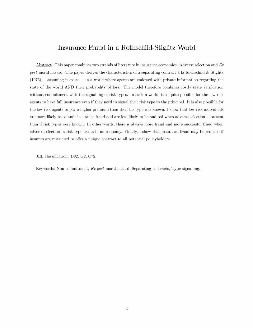
is a sextuplet in this game. Figure 2 is an extensive-form representation of the claiming game.

Let represent the probability that the agent announces a loss when he did not suffer a loss. then

represents the probability that an agent who reported a loss of is audited. Lemma 1 provides the unique

PBNE in mixed equilibrium of this claiming game.

Lemma 1 For each agent type ∈ , the unique PBNE in mixed strategy of this game is such that:1- the agent who suffered a loss always tells the truth; 2- the agent who suffered no loss reports a loss

6

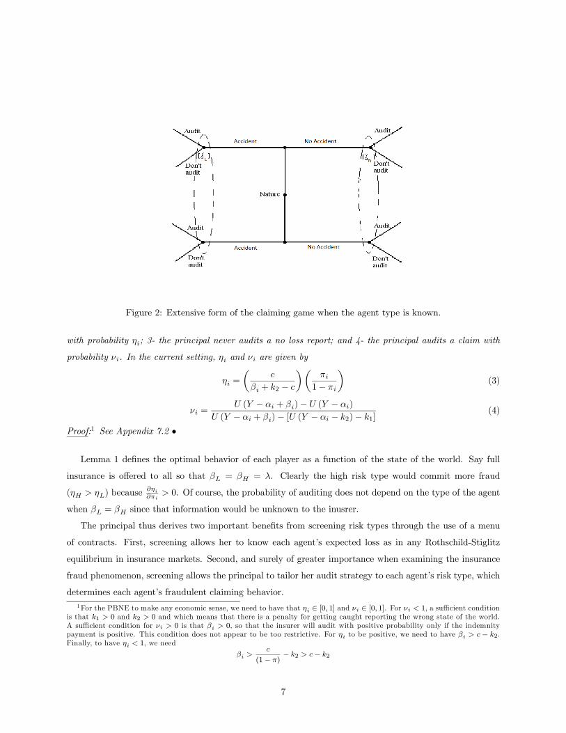
Figure 2: Extensive form of the claiming game when the agent type is known.

with probability ; 3- the principal never audits a no loss report; and 4- the principal audits a claim with

probability . In the current setting, and are given by

=

µ

+ 2 −

¶µ

1−

¶(3)

= ( − + )− ( − )

( − + )− [ ( − − 2)− 1](4)

Proof:1 See Appendix 7.2 •

Lemma 1 defines the optimal behavior of each player as a function of the state of the world. Say full

insurance is offered to all so that = = . Clearly the high risk type would commit more fraud

( ) because

0. Of course, the probability of auditing does not depend on the type of the agent

when = since that information would be unknown to the inusrer.

The principal thus derives two important benefits from screening risk types through the use of a menu

of contracts. First, screening allows her to know each agent’s expected loss as in any Rothschild-Stiglitz

equilibrium in insurance markets. Second, and surely of greater importance when examining the insurance

fraud phenomenon, screening allows the principal to tailor her audit strategy to each agent’s risk type, which

determines each agent’s fraudulent claiming behavior.

1For the PBNE to make any economic sense, we need to have that ∈ [0 1] and ∈ [0 1]. For 1, a sufficient condition

is that 1 0 and 2 0 and which means that there is a penalty for getting caught reporting the wrong state of the world.

A sufficient condition for 0 is that 0, so that the insurer will audit with positive probability only if the indemnity

payment is positive. This condition does not appear to be too restrictive. For to be positive, we need to have − 2.

Finally, to have 1, we need

(1− )− 2 − 2

7

2.3 The Contract for each agent type

There are four variables that must be specified in the menu of contracts: The coverage in case of a loss by

the high risk type (), the coverage in case of a loss by the low risk type (), the premium for the high

risk type (), and the premium for the low risk type ().

2.3.1 The principal’s (participation) zero-profit function

Given the players’ optimal strategies, it is possible to find the insurance premium that gives zero expected

profits to the principal for each agent type. For an agent of type ∈ , this premium is implicitly givenby

= |zIndemnity when loss

+ (1− ) (1− )| z Rent

+ [ + (1− )]| z Cost of audit

+ (1− ) 2| z Monetary penalty

(5)

On the right, represents the expected benefits paid when a type-i agent tells the truth. The second

term, (1− ) (1− ), is the rent an agent can expect to extract from the principal by lying about

the state of the world with probability and not being audited with probability (1− ). The third

term, [ + (1− )], is the expected cost of the auditing strategy that the principal must pass on to

agents. Finally, (1− ) 2, is the expected amount collected by the principal when the agent is caught

committing fraud.

By substituting in (5) for the equilibrium value of given in (3), the price of the contract becomes

= +

µ

+ 2 −

¶=

∙1 +

+ 2 −

¸(6)

This zero-profit constraint has the nice characteristic that it is not related directly to the principal’s

auditing strategy, which also means that it is not related to the agent’s utility function, the agent’s initial

wealth ( ) or the deadweight penalty (1). The term³

+2−

´represents the implicit loading factor of the

insurance contract. This loading factor increases in the cost of auditing , but decreases in the indemnity

payment . From (6), we find that unless = 2, the zero-profit functions associated with the high risk

type crosses the zero-profit function of the low risk type at the points where the indemnity are = 0 and

= −2, so that = 0 in both cases. The low risks’ zero-profit condition lies below the high risks’ for allvalues of 0, as it should be expected.

In contrast to the classic linear zero-profit conditions in Rothschild and Stiglitz (1976), the zero profit

conditions when ex-post moral hazard is present is not necessarily linear. It can also be convex or concave,

and even non-monotonic. The shape of the principal’s zero-profit function depends on the relationship

between the cost of verifying, , and the penalty that is paid to the principal in case the agent is found guilty

of having reported the wrong state of the world, 2 (in other words, is 2 − positive, negative or zero).

Although there are technically three possible cases (depending on Q 2), the most interesting case

occurs when 2. It includes the case where the principal receives nothing from catching the agent telling

8

a lie (i.e., 2 = 0),2 which is more in line with what is observed in reality. This is the case I will concentrate

on in this paper. The other two cases are relegated to Appendix 7.3 and provided only for the sake of

completeness.

Assuming then that 2, the function in (6) reaches an optimum in terms of when

=

+ 2−

(+2−)2= 0. There are two real zeros to the function

= 0: = (− 2) +

p (− 2) 0

and = (− 2) −p (− 2) 0. The first zero (when 0) is a minimum of the function since

we then have 22

= −2 (2−)(+2−)3

0 when 2 and − 2.3 The present exercise allows

us to see that the convexity of the premium function increases with the probability of loss . Figure 3

illustrates the zero-profit premium for the high risk and the low risk agents when − 2 0. The function

Figure 3: Premium functions =

h1 +

+2−ithat give the principal zero profit for the high risk

agent ( = ) and the low risk agent ( = ) when 2. The graph is drawn using the following

parameters: = 20, = 2%, = 5%, = 10, = 2, and 2 = 1. The premium is on the vertical axis

and the coverage is on the horizontal axis.

= + acts as an asymptote that bounds the insurer zero-profit function below for very large

and positive (Figure 4), and as an asymptote that bounds the same function above for largely negative.

The vertical asymptote, whatever the risk type is, is defined by = − 2.

As stated earlier, I shall concentrate only on the situation where 2 ≥ 0 and − 2 0. The

reason is mainly that it is the only situation for which the PBNE found in Lemma 1 has a non-degenerate

2See Bourgeon and Picard (2012) for a more lengthy discussion of the situation where 2 0.3The function is concave when − 2 so that a maximum is reached at the second zero (when = (− 2) +

(− 2) 0) since

22

= −2 (2−)(+2−)3

0 when 2 and − 2

9

Figure 4: For the high risk agent, the premium function =

h1 +

+2−ithat gives the principal

zero profit when 2, and the asymptote that has equation = ( + ). The vertical asymptote

at = − 2 is not displayed but can easily be inferred from the graph. The graph is drawn using the

following parameters: = 20, = 5%, = 10, = 2, and 2 = 1. The premium is on the vertical axis

and the coverage is on the horizontal axis.

solution (i.e., the probability of committing fraud, , and the probability of auditing, , are comprised

between 0 and 1).

2.3.2 The maximization problem

When types are known, the problem for the principal is to choose a coverage and premium pair that maximizes

each agent’s expected utility over final wealth,

max

( − − + ) + (1− ) (1− ) ( − ) (MP)

+(1− ) [ ( − − 2)− 1] + (1− ) ( − + )

subject to the principal’s break-even constraint (6), and the equilibrium probability of filing a fraudulent

claim (3) and of auditing a claim (4). Assuming that the agents’ participation constraint holds (otherwise

there wouldn’t be any insurance fraud problem since there wouldn’t be any insurance), and substituting (3),

(4) and (6) into , the maximization problem simplifies to

max

=

µ −

∙ +

µ

+ 2 −

¶¸− +

¶+(1−)

µ −

∙ +

µ

+ 2 −

¶¸¶(7)

The deadweight penalty (1) is not a factor in the design of the optimal contract. The reason is that

the decision to audit comes last in the sequence of play, so that the deadweight penalty is internalized in

10

the principal’s audit probability. In contrast, the penalty paid to the principal does not have an impact on

the structure of the contract (see also Bourgeon and Picard, 2012). As we can see, the penalty paid to the

principal by the agent in case he is found to have committed fraud (2) reduces the insurance premium paid.

The solution to the ex post moral hazard game without commitment can then be easily solved by finding

the first order condition of problem (7) with respect to . The first order condition can be written as

0³ −

h +

³

+2−´i− +

´

0³ −

h +

³

+2−´i− +

´+(1− )

0³ −

h +

³

+2−´i´ =

Ã1 +

2 −

( + 2 − )2

!(8)

We see that if = , so that the agent is fully insured, then the condition for an optimum becomes

2 −

( + 2 − )2= 0 (9)

which can occur only if 2 = . In other words, provided that insurance is purchased at all, the optimal

contract for the two agents entails full insurance if and only if the penalty paid to the principal is equal to

her auditing cost. I state this result formally in the following proposition.

Proposition 1 In the presence of ex post moral hazard that characterizes insurance fraud, full insurance

is optimal if and only if the penalty paid to the principal in the event the agent is found to have committed

insurance fraud is exactly equal to the principal’s cost of auditing. If the penalty is less (more) than the cost

of auditing, then the optimal indemnity is greater (smaller) than the loss.

Proof. Follows from the previous discussion.•

This proposition tells us that if 2 (the case that is most likely in the economy as it encompasses

the situation where 2 = 0) so that 2−

(+2−)2 0, then more-that-full insurance is optimal (i.e., ),

provided that risk-types are known. Figure 5 presents graphically the solution to this game where risk-types

are known to all players.

In contrast to Boyer (2004), but in line with Bourgeon and Picard (2014), overcompensation of losses

is not solely due to the fact that the principal cannot commit. Partial insurance could occur even in the

presence of principal non-commitment provided that the agent pays a part of his penalty directly to the

principal (i.e., 2 6= 0). The contracts are structured to increase the principal’s incentives to verify the

agents’ report about the state of the world. The impact of the other model parameters on the indemnity

payment is provided in the following corollary.

Corollary 1 In the presence of ex post moral hazard that characterizes insurance fraud, the indemnity

payment increases as the probability of loss increases (

0), the cost of auditing increases (

0) and

the penalty paid to the principal decreases (2

0).

11

Figure 5: Solution to the game when agent types are known. The indemnity payment is on the horizontal

axis and the premium is on the vertical axis. Only the part of the graph where − 2 is represented

here.

Proposition 2 Proof. Writing the first order condition of problem (7) with respect to as

Ω = 0 = 0µ −

∙ +

µ

+ 2 −

¶¸− +

¶Ã1− −

Ã2 −

( + 2 − )2

!!

−(1− )0µ −

∙ +

µ

+ 2 −

¶¸¶Ã1 +

Ã2 −

( + 2 − )2

!!and finding the total derivative of

Ω = 0 =Ω

+

Ω

+

Ω

+

Ω

22

gives us that ³

´=

¡Ω

¢since Ω

0 for ∈ 2. Solving provides the appropriate

result.•

The principal is induced to audit with greater probability by increasing what she has to lose by not

auditing (that is, the indemnity payment and the penalty paid to her if she finds that the agent has

committed fraud 2). When both the indemnity payment and the penalty paid to the principal are larger,

then the incentives for the principal to audit are also larger, which then results in a lower likelihood of

committing fraud. This is even more obvious when we realize that the probability of fraud, , decreases

when both 2 and are larger. Picard (2013) and Bourgeon and Picard (2014) provide more thorough

discussions of this phenomenon.

12

3 Adverse Selection with Non Linear Zero Profit Constraints

Following the Rothschild-Stiglitz tradition, the principal’s objective is to choose a menu of contracts4

(

) such that

max

= ( − − + ) + (1− ) ( − ) (AS)

subject to

( − − + ) + (1− ) ( − ) ≥ ( − − + ) + (1− ) ( − ) (IC)

( − − + ) + (1− ) ( − ) ≥ ( − − + ) + (1− ) ( − ) (IC)

≥

∙ +

µ

+ 2 −

¶¸(ZC)

≥

∙ +

µ

+ 2 −

¶¸(ZC)

( − − + ) + (1− ) ( − ) ≥ ( − ) + (1− ) ( ) (PC)

( − − + ) + (1− ) ( − ) ≥ ( − ) + (1− ) ( ) (PC)

The two incentive compatibility constraints ( and ) stipulate that agents should be better off pur-

chasing the contract that is designed for their own risk type rather than purchasing the contract that is

desinged for the other risk type. The two zero-profit constraints ( and ) are the principal’s zero-

profit constraints for each agent type (see equation 6). Finally the two participations constraints ( and

) stipulate that agents must be better off being insured than in autarchy.

Assuming the principal makes no profit on each contract on average (i.e., equations and hold

with equality), that the two types of agents prefer insurance to autarchy (i.e., equations and are

not binding), and the appropriate single-crossing property for the incentive compatible constraints ( is

not binding, but is), the problem simplifies to

max

=

µ −

∙ +

µ

+ 2 −

¶¸− +

¶(AS0)

+(1− )

µ −

∙ +

µ

+ 2 −

¶¸¶subject to .

The solution to this maximization problem5 is such that

0³ −

h +

³

+2−

´i− +

´⎡⎣

0³ −

h +

³

+2−

´i− +

´+(1− )

0³ −

h +

³

+2−

´i´ ⎤⎦ =Ã1 +

(2 − )

( + 2 − )2

!

4Note that I already substituted the players’ Nash strategies in the objective function and in the participation constraints.

I shall use superscript to refer to the case where agent types can be seperated.5 See the appendix.

13

which is the same solution as when the high risk agent’s type was known (see equation 8). Note that when

2 = 0, the right hand side becomes(

−2)

(−)2 , which means that

2 for there to be a solution.

As in the original Rothschild and Stiglitz (1976) paper, the contract designed for the high risk agents is

not affected by the presence of low risk agents. Rather, it is the low-risk agents who must signal their type

by adapting their behavior and accepting a contract that reflects their lower risk. It is then appropriate to

use the binding constraint to find the value of as a function of

0 =

µ −

∙ +

µ

+ 2 −

¶¸− +

¶+ (1− )

µ −

∙ +

µ

+ 2 −

¶¸¶(10)

−µ −

∙ +

µ

+ 2 −

¶¸− +

¶− (1− )

µ −

∙ +

µ

+ 2 −

¶¸¶Figure 6 illustrates the contracts under adverse selection with a non-linear zero-profit constraint for each

risk type; the horizontal axis represents the indemnity, whereas the premium can be found on the vertical

axis. As we see in the figure, the high risk agent’s utility function, , is such that he purchases a contract

(point ) that is more expensive than the contract offered to the low risk agents (point ) along their

utility function . That is obvious from the fact highlighted earlier that the high risks’ zero profit function

(_) always lies above the low risks’ (_). From the incentive compatibility constraints, we know

that the low risks will signal their type by purchasing a contract (point 0) that provides a lower coverage

than what they would have chosen had their type been known (point ). The low risk agent’s expected

utility in autarchy is given by the dashed line labelled .

An interesting difference between the menu of contracts when ex-post moral hazard and principal non-

commitment are present and the classical Rothschild-Stiglitz menu of contracts is that low risk agents may

have to signal their type by paying a higher premium for this lower level of coverage. And even though this

result depends on the value of the parameters, it represents a new result in the economics of insurance.

The reason why the low-risk type may end up paying a higher premium under adverse selection when

insurance fraud is a possibility is two-fold: First there is the convex nature of the insurer’s zero-profit

constraint, and second there is the decreasing relationship between premium and indemnity. In the classical

Rothschild-Stiglitz world, the insurers’ zero profit condition is a straight line, with = in the case of

the low risk. In the presence of insurance fraud, the zero profit condition becomes

h +

³

+2−´i,

so that the derivative with respect to the indemnity is equal to

h1 + 2−

(+2−)2i. The premium function

reaches a minimum when min = − (2 − ) +p− (2 − ), so that the relationship between indemnity

and premium is negative when − (2 − ) +p− (2 − ).6 Note that the premium function reaches a

minimum at a poin that is independent of the agent’s risk of accident, which means that for a given the

zero-profit function is more convex the higher is the risk of the loss (i.e.,

³22

´ 0) − see Figure 3 for a

6 In other words, 1 + 2−(+2−)2 0 when − (2 − ) +

− (2 − ).

14

Figure 6: Solution to the game when agent types are unknown. The indemnity payment is on the horizontal

axis and the premium is on the vertical axis. The low risk signals his type (function ) by accepting a

lower converage, but a higher premium than when types are knows. The low risk agent’s expected utility in

autarchy is given by the dashed line labelled . The parameter values used for this example are = 20,

= 1%, = 10%, = 2, and 2 = 0. The utility function is ( ) = ln ( ).

better illustration of this relationship between an agent’s risk of a loss and the convexity of the zero-profit

function for that agent.

The question that we may raise at this point is to find the conditions under which the premium paid

by the agent in the presence of adverse selection is greater than the premium he pays in the absence of

adverse selection? To answer this question, it is sufficient to compare =

h +

³

−´i

with

=

h +

³

−´i. Let 2 = 0 for tractability reasons (so that min = 2). Clearly the premium

under adverse selection and ex post moral hazard will be greater than the premium under ex post moral

hazard (i.e., ) if and only if

µ

−

¶

µ

−

¶The function 2

− reaches a minimum at = 2. We also know that must be smaller than ∗ for the

signal to be credible. For ∗ at the same time as

³

−´

³

−´, it must be that 2.

Another way to look at this is to apply the fact that − 0 since low-risk agents need to signal their

type by choosing a lower indemnity payment. It then follows that if and only if

−

15

Whether this is true depends on the value of the parameters. For instance, if is "close" to , then it

is obviously true that the low-risk agent’s premium under adverse selection will be greater than under full

information. The following proposition illustrates the situation.

Proposition 3 In an economy plagued with adverse selection of risk types and with ex post moral hazard,

there exists a difference between each agent’s probability of having an accident (say ∆) such that for all

differences greater than ∆ (or alternatively for all +∆), the low risk agents ends up paying a

greater premium than if his type was known. This is true even if the indemnity payment he receives is lower

under adverse selection than when his risk type is known.

Proof. I want to show the conditions under which . This occurs when

h +

³

−´i

h +

³

−´i, which is the same as finding

− .

We know that − is bounded above at − = 1 and below at − = 0. We know that

when − → 0, so that there is no difference between the different agents’ risk types, then =

h +

³

−´i=

h +

³

−´i= . This means that low risk agent’s premium is the same

under adverse selection as under full information. When − → 1 (so that → 1 at the same time

as → 0) then from Equation 10 it follows that

0 = ( − + )−

µ −

µ

+ 2 −

¶−

¶so that

=

µ

+ 2 −

¶Substituting for =

³

+2−

´in

− , we find that

if and only if

−2 +

which is obviously true since − 2 0. It follows that³

−2

´ = . Consequently

there is a value of ∆ = − ∈ (0 1) such that = . Therefore the premium paid by the low risk

agent in the separating contract is greater than the premium he would have paid had his type been known for

all +∆. •

The proposition essentially shows what Figure 3 alluded to. It shows that when risk types are sufficiently

different, then because of the convex nature of the zero-profit constraints for each agent type in an economy

where agents are able to misrepresent the true state of nature and where the principal cannot commit to an

auditing strategy, the separating equilibrium may be such that the low risk agent’s contract lies in a region

where less coverage is met with a greater premium. This region where greater coverage is met with a lower

premium (that is,

0) is observed when the low risk agent’s coverage is between the principal’s cost of

auditing and twice her cost of auditing (i.e., 2).

16

3.1 Illustration

To illustrate the situation, suppose agents have a CRRA utility function (i.e., () = 1−1− ) with = 3.

Let also = 11, = 10, = 5, 1 = 02, 2 = 0, = 5% and = 10%. In autarchy the low risk agents’

expected utility is −00289 whereas the high risk agents’ expected utility is −00537. The minimum of the

premium function is reached when = 2 = 10. When risk types are known, the solution is such that the

high risks’ expected utility is maximized with contract = 1230; = 20725. The low risks’ expectedutility is maximized with contract = 1235; = 10376. The low risk agents’ expected utility is then−00050 whereas the high risk agents’ expected utility is −00060.When the principal knows the agents’ risk type, then she knows that high risk agents will opt for a

contract that has a less generous coverage. This result contrasts with the one I presented when risk types

and states of the world are public knowledge. Under perfect information the premiums are equal to = 05

and = 10; as the high risk types are twice as likely to have an accident, their premium is twice as

expensive. When the state of the world is private information (i.e., insurance fraud is possible), then the

high risk agents pay a bit less than twice as much as the low risk agents because they purchase a contact

that has smaller indemnity payments than the contract purchased by the low risks.

When risk types are not known, however, the low risk agents will opt for contract = 670; = 13203whereas the high risk agents will obtain the same contract = = 1230;

= = 20725, as when

risk types were known. The low risk agents’ expected utility is then −00057, which is worse than their ex-pected utility in the case of a full type information, but still better than in autarchy.7

It is easy to calculate how much fraud there is in this economy contingent on the scenarios of full type

information and of adverse selection. Let us start with the case where the principal has perfect information

as to the risk type of the agents. Using the equilibrium values of given in (3), fraud probabilities are equal

to = 761% for the high risk agents and to = 358% for the low risk agents. From the equilibrium

value of given in (4), the probability that the principal audits each type of agents is given by = 491%

(in case of the high risk agents) and = 358% (in the case of the low risk agents). We see that the high

risk types are more likely to commit fraud than the low risk types. We also see that the high risk agents

are more likely to be audited than the low risk agents. Under adverse selection the high risk’s probability

of fraud and probability of being audited remain the same so that = and = , whereas the low

risk’s probability of fraud increases to = 1559% 358% = at the same time as their probability of

being audited decreases to = 336% 358% = . Given that the high risk agents do not change their

7 It is easy to calculate how much fraud there is in this economy contingent on the scenarios of full type information and

of adverse selection. Let us start with the case where the principal has perfect information as to the risk type of the agents.

Using the equilibrium values of given in (3), fraud probabilities are equal to = 761% for the high risk agents and to

= 358% for the low risk agents. From the equilibrium value of given in (4), the probability that the principal audits each

type of agents is given by = 491% (in case of the high risk agents) and = 388% (in the case of the low risk agents).

We see that the high risk types are more likely to commit fraud than the low risk types. We also see that the high risk agents

are more likely to be audited than the low risk agents.

17

equilibrium behavior when adverse selection is present (because the parameters of their insurance contract

do not change), the only difference in the amount of fraud in the economy muast come from the low risk

agents’ behavior only.

In this example the incentive compatible contract offered to the low risk agents is such that the low risk

agents end up paying a higher premium than when the principal knew the agents’ type. Consequently, when

adverse selection is present in a costly verification context without commitment, then type signalling can

occur through a lower indemnity payment, AND a higher premium.

3.2 Separation and Fraud

When adverse selection is present in the sense that only the agents know their own risk type, then the high

risk type’s probability of fraud and the principal’s probability of auditing a high risk agent remain the same

since the contract for the high risk agent in the Rothschild-Stiglitz economy is the same as when his risk

type is known. This means that if adverse selection has any impact on the amount of fraud in the economy,

it must come from its impact on the low-risk agents’ behavior.

It is interesting to see that the amount of fraud in the economy increases because of adverse selection.

The total amount of fraud in the economy when types are known is given by

= (1− ) + (1− ) (1− )

=

µ

+ 2 −

¶+ (1− )

µ

+ 2 −

¶When an agent’s type is private information, the total amount of fraud will be given by

=

µ

+ 2 −

¶+ (1− )

µ

+ 2 −

¶We are then able to conclude with the following proposition.

Proposition 4 When adverse selection is present in an economy, then insurance fraud, as defined by the

filing of a claim when there was no loss, is increased and the probability of a successful fraudulent claim is

also increased.

Proof. The optimal menu of contracts is such that = . This means that if and

only if

³

+2−

´

³

+2−´. This occurs when , which we know to be true since the

low risk type needs to signal that he is low risk by accepting a contract that offers less coverage. Consequently

adverse selection in risk types leads to an economy where insurance fraud is more prevalent. At the same

time as the low risk agent’s probability of fraud increases when adverse selection is present (i.e., ),

the probability of auditing a low-risk agent is reduced (i.e., ). To see why, note that

0 so that

as the low risk must signal its type by choosing a contract that provides a smaller coverage than when types

are known. •

18

Because of adverse selection, low-risk agents are more likely to commit fraud AND are less likely to be

audited when they file a claim. This means that low-risk agents are more likely to be successful in committing

fraud when adverse selection is present than when types are known.

4 The Pooling Contract

One can wonder whether a pooling contract can survive cream skimming. In habitual settings, pooling

equilibriums are not stable because of the single crossing property.8 It is still the case here (see Figure 5

for a more obvious situation). Consequently, no pooling contract is sustainable in a competitive equilibrium

because it is always possible to design a contract that would attract only the low risk individuals (see Snow,

2009, and Mimra and Wambach, 2011, and the references9 therein for a more thorough discussion). This

means that there is a potential side payment à la Miyazaki-Spence that could increase the welfare of all the

agents in the economy compared to the pooling contract. Instead of entering that debate, I would rather

examine what happens to the amount of insurance fraud if, for some reason, insurers are not allowed to offer

separating contracts.

First note that the claiming game changes because the principal can no longer separate the high risk from

the low risk individual, meaning that she will not be able to condition her auditing strategy on the agent’s

type. This means that the extensive form of the game changes to become like that of Figure 7. The solution

to this PBNE is provided in the appendix. For the purpose of the remainder of the paper, I will limit my

discussion to the case where the parameter values give us an interior solution in the sense that ∈ (0 1)and ∈ (0 1).Given that only one contract is offered in this game, the principal does not know if a given contract is

acquired by an agent whose probability of having an accident is low or high. She does know, however, that

proportion of low risk agents in the economy is given by . When time comes for the principal to investigate

or not, the only thing she knows is whether the agent announced he suffered a loss or not. She does not

know if the agent is of a low-risk or of a high-risk category, or if the report is truthful or not. Irrespective

of the agent’s type, it is clear that if the agent does not claim any loss then the principal’s optimal strategy

is to not investigate.

Substituting for the PBNE constraints that are available in the appendix, the insurer faces the following

maximization problem when a single contract must be offered to all policyholders in the economy:

max

= ¡ − − +

¢+ (1− ) ( − )

8As Mimra and Wambach (2012) put it: "In the classic RS model with two risk types, the high risk indifference curve is

always flatter than the lowrisk indifference curve, as the high risk is always willing to pay more for one more unit of further

insurance compared to the lowrisk" (p. 3).9 Including Smart (2000), Villeneuve (2003) and Wambach (2000).

19

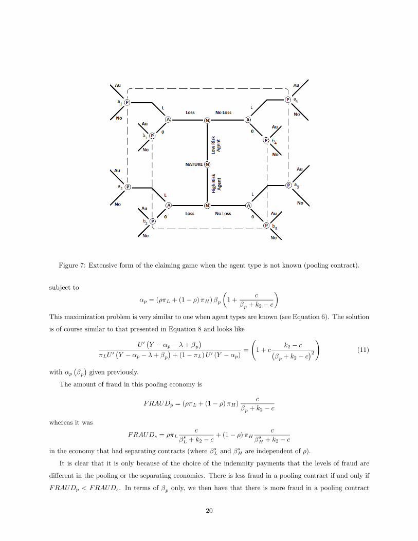
Figure 7: Extensive form of the claiming game when the agent type is not known (pooling contract).

subject to

= ( + (1− ))

µ1 +

+ 2 −

¶This maximization problem is very similar to one when agent types are known (see Equation 6). The solution

is of course similar to that presented in Equation 8 and looks like

0¡ − − +

¢ 0

¡ − − +

¢+ (1− ) 0 ( − )

=

Ã1 +

2 − ¡ + 2 −

¢2!

(11)

with ¡¢given previously.

The amount of fraud in this pooling economy is

= ( + (1− ))

+ 2 −

whereas it was

=

+ 2 − + (1− )

+ 2 −

in the economy that had separating contracts (where and are independent of ).

It is clear that it is only because of the choice of the indemnity payments that the levels of fraud are

different in the pooling or the separating economies. There is less fraud in a pooling contract if and only if

. In terms of only, we then have that there is more fraud in a pooling contract

20

provided that

+ (1− )

+2− + (1− )

+2−

− 2 + (12)

or

³1

+2−

´ + (1− )

³1

+2−

´

³1

+2−

´+ (1− )

³1

+2−

´ (13)

Whether there is more or less fraud in the economy where contracts are mandated to be equal for all

participants depends on the proportion of low risk agents () in the economy. As becomes smaller, the

likelihood of having more fraud in the pooling economy increases since it reduces the likelihood that the

previous equality holds. I state this results as our last proposition.

Proposition 5 In an economy where insurers are restricted from offering a separating menu of contracts,

the amount of insurance fraud committed will be smaller than in an economy where agents who face different

risks self-select into different contracts provided that the proportion of low risk individuals is greater than

some proportion ∗.

Proof. We know that as → 0, then the right hand side of Equation 12 converges to . We know

that . Similarly as → 1, then the right hand side of Equation 12 converges to . We know that

. So we have that as → 0 there is more fraud with a pooling contract (i.e., )

whereas as → 1 there is more fraud with a separating contract (i.e., ). There must

therefore exist a ∗ ∈ (0 1) such that = . This is made more clear by the fact that the

right hand side of Equation 12 is monotone and decreasing in so that

⎛⎝

³1

+2−

´ + (1− )

³1

+2−

´

³1

+2−

´+ (1− )

³1

+2−

´⎞⎠ 0 (14)

if and only if

−µ

1

+ 2 −

¶µ1

+ 2 −

¶( − ) 0

which is obviously true since . •

Let us illustrate the situation using the same basic example as before. Let there be agents with CRRA

utility functions whose coefficient of risk aversion is = 3. Let also be the following parameters = 11,

= 10, = 5, 1 = 02, 2 = 0, = 5% and = 10%. In the case of the separating equilibrium, the

low risk chooses contract ( = 670 ; = 13203), whereas the high risk chooses contract (

= 1230 ;

= 20725).

In the pooling of types, with = 50%, both agents receive contract ( = 1159 ; = 15290). Given

the parameters of the economy, the condition for having less fraud in the pooling economy is respected since

the right hand side of Equation 13 is equal to 86621. This is clearly less than = 1159. For smaller values

21

of , say = 5%, the inequality in Equation 13 does not hold. The pooling contract is such that ( = 1123

; = 19736). The right hand side of Equation 13 is itself equal to 1180. Clearly this is greater than the

left hand side, = 1123. Consequently, there is more fraud with this pooling contract when is small; and

of course there is less fraud under a unique contract when is large.

5 Discussion and Conclusion

This paper re-examines the traditional Rothschild-Stiglitz separating insurance contract in the presence of

insurance fraud. I modelled insurance fraud in this paper as a non-cooperative game between a principal

(the insurance company), who cannot commit credibly to an auditing strategy, and twice-privately informed

agents (the policyholdert) in the sense that they privately know their probability of loss (which can be high

or low) AND they privately observe what is the state of the world (i.e., what loss did they suffer). In a

two-point distribution of states of the world (loss and no loss), I confirm that the optimal separating contract

entails overpayment of the loss for the high risk type, provided that the penalty paid by the agent to the

principal in the event he is caught committing fraud is smaller than the principal’s cost of auditing.

For the low risk type, the results are more convoluted. The low-risk agents receive a contract that is

not as good as the contract that they would have chosen had their risk types been known. Low-risk agents

may still receive a contract that provides full insurance in the sense that the indemnity payment is equal

to their potential loss. Also, depending on the parameter values, low-risk agents may end up in a situation

in which, compared to the situation where their risk type was known, they choose a contract that has a

lower indemnity payment AND a higher premium. This higher premium is due of course to the problem of

insurance fraud in the economy. To my knowledge, the insurance fraud phenomenon has not been studied in

an adverse selection setting à la Rothschild-Stiglitz before. I show that insurance fraud is more prevalent in

the presence of adverse selection because low-risk agents must accept a lower indemnity payment in order to

signal their risk type. As insurance fraud is negatively linked to the indemnity payment, a lower indemnity

payment is associated with more fraud. Moreover, the probability of auditing is decreased in the presence

of adverse selection.

I also examined the situation of contract restrictions in the sense that I looked at the situation where

insurers are mandated to offer a single contract to every one. This pooling contract is, of course, unstable

in the setting as it was shown in many papers. This means that similar to the situation encountered in the

Rothschild-Stiglitz setup, there is a wide range of parameter values such that all agents in the economy would

prefer the pooling contract situation to the separating contract situation. But once the pooling contract is

offered, there are alternate contracts that would attract low-risk agents, but not the high-risk agents and

make a positive profit. This discussion about inefficient and second-best contracts notwithstanding, and

assuming instead that the government restricts the possibility of offering a menu of contracts, I showed that

22

provided the proportion of high-risk agents is low enough, then the amount of fraud in the economy can be

smaller when all agents are forced into a single contract that makes zero profit.

23

6 References

1. Bond, E. W. and K. J. Crocker (1997). Hardball and the Soft Touch: The Economics of Optimal

Insurance Contracts with Costly State Verification and Endogenous Monitoring. Journal of Public

Economics, 63: 239-254.

2. Bourgeon, J.-M. and P. Picard (2014). Fraudulent Claims and Nitpicky Insurers. American Economic

Review, 104(9): 2900-2917.

3. Boyer, M. M. (2000). Centralizing Insurance Fraud Investigation. Geneva Papers on Risk and Insurance

Theory, 25: 159-178.

4. Boyer, M. M. (2004). Overcompensation as a Partial Solution to Commitment and Renegotiation

Problems: The Case of Ex-post Moral Hazard. Journal of Risk and Insurance, 71: 559-582.

5. Boyer, M. M. (2007). Resistance (to Fraud) is Futile. Journal of Risk and Insurance, 74: 461-492.

6. Gale, D. and M. Hellwig (1985). Incentive-Compatible Debt Contracts: The One-Period Problem.

Review of Economic Studies, 52:647-663.

7. Graetz, M. J., J. F. Reinganum and L. L. Wilde (1986). The Tax-Compliance Game: Toward an

Interactive Theory of Law Enforcement. Journal of Law, Economics and Organization, 2: 1-32.

8. Khalil, F. (1997). Auditing without Commitment. Rand Journal of Economics, 28: 629-640.

9. Krasa, S. and A.P. Villamil (2000). Optimal Contracts When Enforcement is a Decision Variable.

Econometrica, 68: 119-134.

10. Mimra, W. and A. Wambach (2011). A Game-Theoretic Foundation for the Wilson Equilibrium in

Competitive Insurance Markets with Adverse Selection. CESifo Working Paper Series No. 3412,

http://papers.ssrn.com/sol3/papers.cfm?abstract_id=1808672.

11. Mimra, W. and A. Wambach (2012). Profitable contract menus in competitive insurance markets with

adverse selection. Mimeo, Risk Theory Society

12. Mookherjee, D. and I. Png (1989). Optimal Auditing, Insurance and Redistribution. Quarterly Journal

of Economics, 104: 205-228.

13. Picard, P. (1996). Auditing Claims in the Insurance Market with Fraud: The Credibility Issue. Journal

of Public Economics, 63: 27-56.

14. Picard, P. (2013). Economic Analysis of Insurance Fraud. In The Handbook of Insurance, Georges

Dionne editor. Kluwer Academic Publishers, forthcoming.

15. Rothschild, M. and J.E. Stiglitz (1976). Equilibrium in competitive insurance markets: an essay on

the economics of imperfect information. Quarterly Journal of Economics, 90: 630-649.

16. Smart, M., (2000). Competitive insurance markets with two unobservables. International Economic

Review 41: 153—169.

17. Snow, A., (2009). On the possibility of profitable self-selection contracts in competitive insurance

markets. Journal of Risk and Insurance 76: 249—259.

18. Townsend, R. M. (1979). Optimal Contracts and Competitive Markets with Costly State Verification.

Journal of Economic Theory, 21: 265-293.

19. Villeneuve, B. (2003). Concurrence et antiselection multidimensionnelle en assurance. Annales d’Economie

et de Statistique 69: 119—142.

20. Wambach, A. (2000). Introducing heterogeneity in the Rothschild-Stiglitz model. The Journal of Risk

and Insurance 67: 579—591..

24

7 Appendix

7.1 Tables

Table A. Summary of all the variables used in this paper

Variable name Definition

Each agent’s initial wealth

Size of the potential loss

Probability of an accident occurring for the low risk agent

Probability of an accident occurring for the high risk agent

Indemnity to be paid in the contract designed for the low risk agent

Indemnity to be paid in the contract designed for the high risk agent

Premium in the contract designed for the low risk agent

Premium in the contract designed for the high risk agent

Low risk agent’s probability of committing fraud

High risk agent’s probability of committing fraud

Principal’s probability of auditing provided the "low risk contract" is purchase

Principal’s probability of auditing provided the "high risk contract" is purchase

Principal’s cost of auditing an agent’s report

1 Deadweight penalty paid by the agent for committing fraud

2 Penalty paid by the agent to the principal for committing fraud

Table B. Payoffs to an agent of type (i.e., an agent who has a probability of loss ) and to the principal.

State of

the world

Action of

Agent i

Action of

Principal

Payoff to

Agent i

Payoff to

Principal

No accident Tell truth Audits U (Y − ) −cNo accident Tell truth Does not audit ( − ) No accident Lie Audits ( − − 2)− 1 + 2 −

No accident Lie Does not audit ( − + ) − Loss Tell truth Audits ( − − + ) − −

Loss Tell truth Does not audit ( − − + ) − Loss Lie Audits U (Y − −+−k2)−k1 −+k2−cLoss Lie Does not audit U (Y − −)

Payoffs are contingent on the state of the world and on each player’s action.

States in italics represent actions that are off the equilibrium path.

7.2 Proofs

7.2.1 Solution to the claiming game when the agent type is known (Lemma 1, see Boyer, 2000).

From the left-hand side of figure 2, it is clear that 0, the principal’s posterior belief that the agent suffered

a loss given that the agent sent message = 0, is zero. Suppose Nature chooses there to be an accident.

Sending message = then always dominates sending message = 0, whatever the principal does. Also,

if the principal hears message = 0, then she knows for sure that she is not playing at the upper node of

25

left information set. Consequently the only meaningful strategy for the principal is never to audit since she

collects − if she does, and 0 if she does not. Let’s now move to the right side of figure 2.Let be the probability (in the mixed-strategy sense) that the agent sends message = when Nature

chooses there to be a loss. By Bayes’ rule it follows that , the principal’s posterior belief that the reported

loss is real is given by

=

+ (1− )

Only one strategy on the part of the agent makes the principal indifferent as to whether to audit or not.

That strategy must be such that

= + 2 −

+ 2

Isolating in the two previous equation gives

=

µ

+ 2 −

¶µ

1−

¶All that is left to calculate is the principal’s strategy at information set 1.H. Her strategy must be such that

the agent is indifferent between telling the truth and lying, given that = 0. Let be the probability (in a

mixed-strategy sense) of auditing a = message. then solves

( − ) = [ ( − − 2)− 1] + (1− ) ( − + )

which means that

= ( − + )− ( − )

( − + )− ( − − 2) + 1

All six elements of the PBNE have been found.

7.2.2 Solution to the R-S menu of seperating contract.

Rewriting the problem as

max

=

µ −

∙ +

µ

+ 2 −

¶¸− +

¶+(1− )

µ −

∙ +

µ

+ 2 −

¶¸¶

−⎡⎣

h³ −

h +

³

+2−

´i− +

´−

³ −

h +

³

+2−

´i− +

´i+(1− )

h³ −

h +

³

+2−

´i´−

³ −

h +

³

+2−

´i´i ⎤⎦the first order conditions become

: 0 = −

⎡⎢⎢⎣µ(1− ) − 2

(2−)(+2−)

2

¶ 0³ −

h +

³

+2−

´i− +

´−µ(1− ) + (1− )

(2−)(+2−)

2

¶ 0³ −

h +

³

+2−

´i´⎤⎥⎥⎦

26

: 0 =

Ã1−

"1 +

(2 − )

( + 2 − )2

#! 0µ −

∙ +

µ

+ 2 −

¶¸− +

¶

−(1− )

Ã

"1 +

(2 − )

( + 2 − )2

#! 0µ −

∙ +

µ

+ 2 −

¶¸¶

+

⎡⎢⎢⎣

µ1−

∙1 +

(2−)(+2−)

2

¸¶ 0³ −

h +

³

+2−

´i− +

´−(1− )

µ

∙1 +

(2−)(+2−)

2

¸¶h 0³ −

h +

³

+2−

´i´i⎤⎥⎥⎦

: 0 =

h³ −

h +

³

+2−

´i− +

´−

³ −

h +

³

+2−

´i− +

´i+(1− )

h³ −

h +

³

+2−

´i´−

³ −

h +

³

+2−

´i´iso that we find

= −

µ1−

∙1 +

(2−)(+2−)

2

¸¶ 0³ −

h +

³

+2−

´i− +

´−(1− )

µ

∙1 +

(2−)(+2−)

2

¸¶ 0³ −

h +

³

+2−

´i´⎡⎢⎢⎣

µ1−

∙1 +

(2−)(+2−)

2

¸¶ 0³ −

h +

³

+2−

´i− +

´−(1− )

µ

∙1 +

(2−)(+2−)

2

¸¶h 0³ −

h +

³

+2−

´i´i⎤⎥⎥⎦

7.2.3 Solution to the claiming game when the agent type is not known (pooling contract).

The principal’s beliefs has to where she is in the game are given by

1 = 0

2 = 0

3 =(1− ) (1−

)

(1− ) (1− ) + (1−

)

4 = (1−

)

(1− ) (1− ) + (1−

)

When a benefit is requested, her beliefs are given as

1 =

( + (1− ) ) + (1− ) ( + (1− )

)

2 =(1− )

( + (1− ) ) + (1− ) ( + (1− )

)

3 =(1− ) (1− )

( + (1− ) ) + (1− ) ( + (1− )

)

4 = (1− )

( + (1− ) ) + (1− ) ( + (1− )

)

27

For the principal to be indifferent between investigating or not when a loss is claimed, the probability

she assigns to a claim being fraudulent (3 + 4) must solve¡−− ¢(1 + 2) + (2 − ) (3 + 4) = − (15)

where the left hand side represents the principal’s expected payoff from investigating (at nodes 1 and 2

the report is truthful so the principal has to pay the cost of auditing and the claim), and the right hand side

is her payoff from not investigating. Using (15), the belief that fraud is committed is equal to

3 + 4 =

µ

+ 2

¶These beliefs are consequent with fraud probabilities that respect the following condition:

=

µ + (1− )

(1− )

¶

+ 2 − +(1− ) (1− )

(1− )

which is compatible with the fraud probabilities

=

=

µ + (1− )

1− − (1− )

¶

+ 2 −

so that all agents commit fraud with the same intensity, which I will note . Note that this pooled probability

of fraud is larger (resp. smaller) than the low risk’s (resp high risk’s) probability of fraud if types were known

(i.e., ).

For the agents to be indifferent between committing fraud or not when a loss is not observed, it must be

such that

¡ − +

¢+ (1− ) [ ( − − 2)− 1] = ( − )

This gives us that the principal investigates with probability

=¡ − +

¢− ( − )

¡ − +

¢− ( − − 2) + 1

The principal’s beliefs given that a loss was filed are given by

1 =

¡ + (1− )

¢+ (1− )

¡ + (1− )

¢=

³+(1−)1−−(1−)

´

+2− + [ + (1− ) ]³1−

³+(1−)1−−(1−)

´

+2−´

=

µ

+ (1− )

¶µ + 2 −

+ 2

¶

2 =(1− )

( + (1− ) ) + (1− ) ( + (1− ) )

=

µ(1− )

+ (1− )

¶µ + 2 −

+ 2

¶

28

3 =(1− ) (1− )

( + (1− ) ) + (1− ) ( + (1− ) )

=(1− ) (1− )

+ (1− )

µµ + (1− )

1− − (1− )

¶

+ 2 −

¶µ + 2 −

+ 2

¶=

µ(1− ) (1− )

1− − (1− )

¶µ

+ 2

¶

4 = (1− )

( + (1− ) ) + (1− ) ( + (1− ) )

=

µ (1− )

1− − (1− )

¶µ

+ 2

¶To summarize, the beliefs of the principal in each information node are

1 =

µ

+ (1− )

¶µ + 2 −

+ 2

¶; 2 =

µ(1− )

+ (1− )

¶µ + 2 −

+ 2

¶

3 =

µ(1− ) (1− )

1− − (1− )

¶µ

+ 2

¶; 4 =

µ (1− )

1− − (1− )

¶µ

+ 2

¶1 = 2 = 0; 3 = 1− ; 4 =

7.2.4 The simplification of the maximization problem when a pooling contract exists

The problem faced by the principal is

max

¡ − − +

¢+ (1− )

¡1−

¢ ( − )

+ (1− ) [ ( − − 2)− 1] + (1− ) (1− )¡ − +

¢subject to the principal’s zero profit constraint

= £ + (1− ) (1− ) +

£ + (1− )

¤− (1− ) 2¤

+(1− )£ + (1− ) (1− ) +

£ + (1− )

¤− (1− ) 2¤

and the players’ PBNE strategies

=

µ + (1− )

1− − (1− )

¶

+ 2 −

=¡ − +

¢− ( − )

¡ − +

¢− ( − − 2) + 1

Substituting for the PBNE constraints into the maximization problem and the zero profit constraint

yields

max

= ¡ − − +

¢+ (1− ) ( − )

subject to

= ( + (1− ))

µ + 2

+ 2 −

¶

29

7.3 Relationship between audit cost and penalty.

Suppose that = 2, so that the penalty paid by the fraudulent agent to the principal compensates her for

the cost incurred in conducting such an audit. This penalty does not compensate the principal completely

for all audits she conducts, however, since she is compensated only for those audits where she catches

an agent committing fraud. In contrast to the total cost of the principal’s auditing strategy given by

[ + (1− )] (see equation 5) the amount she receives is (1 − ). The principal’s zero-profit

function becomes =

h1 +

i= + , which is nothing more than the premium function when

the loading is fixed and equal to . The two linear zero-profit functions then cross at point ( ) = (− 0).If this is the case, we know that the optimal contract will be full insurance provided any insurance is

purchased. Although the economic importance of this situation is not trivial, it does not represent a result

that warrants more space in this paper.

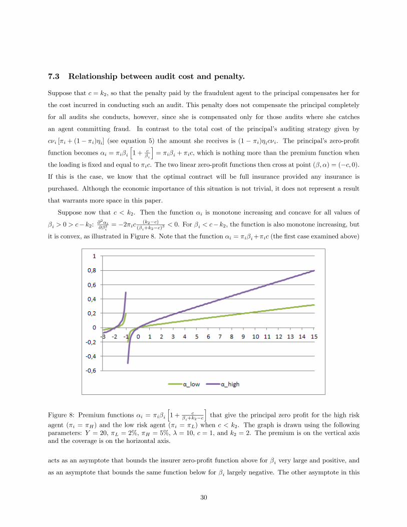
Suppose now that 2. Then the function is monotone increasing and concave for all values of

0 − 2:22

= −2 (2−)(+2−)3

0. For − 2, the function is also monotone increasing, but

it is convex, as illustrated in Figure 8. Note that the function = + (the first case examined above)

Figure 8: Premium functions =

h1 +

+2−ithat give the principal zero profit for the high risk

agent ( = ) and the low risk agent ( = ) when 2. The graph is drawn using the following

parameters: = 20, = 2%, = 5%, = 10, = 1, and 2 = 2. The premium is on the vertical axis

and the coverage is on the horizontal axis.

acts as an asymptote that bounds the insurer zero-profit function above for very large and positive, and

as an asymptote that bounds the same function below for largely negative. The other asymptote in this

30

case is vertical and delimited as = − 2. This situation is illustrated in Figure 9 for the case of the low

risk agent.

Figure 9: For the low risk agent, the premium function =

h1 +

+2−ithat gives the principal

zero profit when 2, and the asymptote that has equation = ( + ). The vertical asymptote

at = − 2 is not displayed but can easily be inferred from the graph. The graph is drawn using the

following parameters: = 20, = 2%, = 10, = 1, and 2 = 2. The premium is on the vertical axis

and the coverage is on the horizontal axis.

31

We know that =∗±

(∗)

2−4∗2

2, which can only occur when±q(∗)

2 − 4∗ 4−∗ . Obviously, we need ∗ (

∗ − 4) 0, which can be achieved when ∗ 0, or when

∗ 4. We then have

∗ ±q(∗)

2 − 4∗2

∗

(∗ − )

if and only if

±q(∗)

2 − 4∗ 2∗

(∗ − )−∗ (16)

This is true whenever

∗

∙±q(∗)

2 − 4∗¸−

∙±q(∗)

2 − 4∗¸ 2

∗ −∗

∗ + ∗

Assume we take the positive root, we then haveµ∗ − 2+

q(∗)

2 − 4∗¶∗

µ∗ +

q(∗)

2 − 4∗¶

whereas if we take the negative root we haveµ∗ − 2−

q(∗ − 2)2 − 4 ()2

¶∗

µ∗ −

q∗ (

∗ − 4)

¶Assume that ∗ 0, then

• Taking the positive root always gives usµ∗ − 2+

q(∗)

2 − 4∗¶ 0 and

µ∗ +

q(∗)

2 − 40 since so that ∗ if and only if

∗

⎛⎝ ∗ +q(∗)

2 − 4∗

∗ − 2+q(∗)

2 − 4∗

⎞⎠which is obviously true since we found that ∗ 2 when there is no adverse selection and

Ã∗+

(∗)

2−4∗∗

−2+

(∗)

2−4∗

1. To see why, note that ∗ +q(∗)

2 − 4∗ ∗ −2+q(∗)

2 − 4∗ since0 −2.

• Taking the negative root always gives usµ∗ − 2−

q(∗)

2 − 4∗¶ 0 and

µ∗ −

q(∗)

2 − 40 so that ∗ if and only if

∗

⎛⎝ ∗ −q(∗)

2 − 4∗

∗ − 2−q(∗)

2 − 4∗

⎞⎠which is obviously true since we found that ∗ 2 when there is no adverse selection and

Ã∗−

(∗)

2−4∗∗

−2−

(∗)

2−4∗1.

32

Assume that ∗ 0 so that ∗ 4. Then

• Taking the negative root always gives usµ∗ − 2−

q(∗)

2 − 4∗¶ 0 and

µ∗ −

q(∗)

2 − 40 so that ∗ if and only if

∗

⎛⎝ ∗ +q(∗)

2 − 4∗

∗ − 2+q(∗)

2 − 4∗

⎞⎠

Given that

Ã∗−

(∗)

2−4∗∗

−2−

(∗)

2−4∗

! 2 (to see why, note that∗−

q(∗)

2 − 4∗

2∗ − 4− 2q(∗)

2 − 4∗, so that 0 −4

• Taking the positive root always gives usµ∗ − 2+

q(∗)

2 − 4∗¶ 0 and

µ∗ +

q(∗)

2 − 40 so that ∗ if and only if

∗

⎛⎝ ∗ +q(∗)

2 − 4∗

∗ − 2+q(∗)

2 − 4∗

⎞⎠

which is obviously true since we found that ∗ 2 when there is no adverse selection and

Ã∗+

(∗)

2−4∗∗

−2+

(∗)

2−4∗1.

• Taking the positive root and squaring on both sides gives us

(∗)2 − 4∗

µ2

∗(∗ − )

¶2− 4 ∗

(∗ − )∗ + (

∗)

2(17)

Assume that ∗ 0 so that the determinant is always positive.

• Taking the negative root always gives us an equation 16 that holds

• Taking the positive root and squaring on both sides gives us

(∗)2 − 4∗

µ2

∗(∗ − )

¶2− 4 ∗

(∗ − )∗ + (

∗)

2(18)

which becomes

∗ (∗)

2

∗ −

after simplification. This inequality is clearly true since we assumed ∗ 0 to start with and ∗ .

Assume now that ∗ 0. We then need ∗ 4 for the determinant to make any sense.

33

• Taking the positive root and squaring (as in equation 18) yields again

∗ (∗)

2

∗ −

This is possible if and only if

∗ − ∗∗ + (

∗)2 0

∗ =∗ ±

q(∗)

2 − 4∗2

∗ =±q(∗)

2 − 4∗ 2−∗

Given that ∗ 4, we would like to find the conditions under which

0 (∗)2 − 4∗ + 42 = (∗ − 2)2

which is impossible.

• Taking the negative root means that

−q−∗ (4−∗) 4−∗ 0

if and only if −∗ (4−∗) (4−∗)2 0. Dividing everywhere by 4− ∗ 0

gives us a solution whereby

0 if and only if 0 4, which is obviously always true.

34