Instructions for use

Title Simulation of high concentration of iron in dense shelf water in the Okhotsk Sea

Author(s) Uchimoto, Keisuke; Nakamura, Tomohiro; Nishioka, Jun; Mitsudera, Humio; Misumi, Kazuhiro; Tsumune, Daisuke;Wakatsuchi, Masaaki

Citation Progress in Oceanography, 126: 194-210

Issue Date 2014-08

Doc URL http://hdl.handle.net/2115/56621

Type article (author version)

File Information Uchimoto_etal_final.pdf

Hokkaido University Collection of Scholarly and Academic Papers : HUSCAP

1

Simulation of high concentration of iron in dense shelf water in 1

the Okhotsk Sea 2

3

Keisuke Uchimotoa, 1), Tomohiro Nakamurab), Jun Nishiokac), Humio 4

Mitsuderad), Kazuhiro Misumie), Daisuke Tsumunef) , Masaaki Wakatsuchig) 5

6

a) Institute of Low Temperature Science, Hokkaido University, N19W8, Sapporo, 7

060-0819, Japan. E-mail: uchimoto@rite.or.jp 8

b) Institute of Low Temperature Science, Hokkaido University, N19W8, Sapporo, 9

060-0819, Japan. E-mail: nakamura@lowtem.hokudai.ac.jp 10

c) Institute of Low Temperature Science, Hokkaido University, N19W8, Sapporo, 11

060-0819, Japan. E-mail: nishioka@lowtem.hokudai.ac.jp 12

d) Institute of Low Temperature Science, Hokkaido University, N19W8, Sapporo, 13

060-0819, Japan. E-mail: humiom@lowtem.hokudai.ac.jp 14

e) Environmental Science Research Laboratory, Central Research Institute of Electric 15

Power Industry, 1646 Abiko, 270-1181, Japan. E-mail: misumi@criepi.denken.or.jp 16

f) Environmental Science Research Laboratory, Central Research Institute of Electric 17

Power Industry, 1646 Abiko, 270-1181, Japan. E-mail: tsumune@criepi.denken.or.jp 18

g) Institute of Low Temperature Science, Hokkaido University, N19W8, Sapporo, 19

060-0819, Japan. E-mail: masaakiw@lowtem.hokudai.ac.jp 20

21

1) Present address: Research Institute of Innovative Technology for the Earth, 22

9-2, Kizugawadai, Kizugawa, 619-0292, Japan. 23

24

25

Corresponding author: 26

Keisuke Uchimoto 27

Research Institute of Innovative Technology for the Earth 28

9-2, Kizugawadai, Kizugawa, 619-0292, Japan. 29

TEL: +81-774-75-2312 30

E-mail: uchimoto@rite.or.jp 31

32

2

33

Keywords: Sea of Okhotsk; iron; simulation; DSW; sedimentary iron 34

35

36

3

Abstract 37

An ocean general circulation model coupled with a simple biogeochemical model was 38

developed to simulate iron circulation in and around the Sea of Okhotsk. The model has 39

two external sources of iron: dust iron at the sea surface and sedimentary iron at the 40

seabed shallower than 300 m. The model represented characteristic features reasonably 41

well, such as high iron concentration in the dense shelf water (DSW) and its mixing, 42

which extends southward in the intermediate layer from the northwestern shelf along 43

Sakhalin Island and finally flows into the Pacific. Sensitivity experiments for the 44

solubility of dust iron in seawater suggest that a solubility of 1% is appropriate in our 45

simulation. Higher solubilities (5% and 10%) result in too low phosphate in the 46

northwestern North Pacific in summer as well as too high iron concentrations at the sea 47

surface, compared with observations. Besides, these experiments show that dust iron 48

hardly contributes to the high iron concentration in the intermediate layer. To 49

investigate locations from which the iron in the intermediate layer originates, the fate 50

of sedimentary iron input from four regions in the Okhotsk Sea was examined. Results 51

suggest that the western and central parts of the northern shelf are important. 52

53

4

1 Introduction 54

The Sea of Okhotsk (Fig. 1) has attracted the attention of oceanographers as an 55

important source region of iron, particularly since Nishioka et al. (2007) hypothesized 56

that the northern part of the Sea of Okhotsk is a main source region of iron to the 57

western subarctic Pacific, which is one of the characteristic areas having high-nutrient 58

and low-chlorophyll (HNLC) owing to iron deficiency (Tsuda et al., 2003; Tsuda et al., 59

2007). The hypothesis of Nishioka et al. (2007) has been confirmed by Nishioka et al. 60

(2014), whose observational data clearly show that a large amount of iron is transported 61

with dense shelf water (DSW) through the intermediate layer. In addition, they showed 62

that iron is vertically homogeneous at the Bussol’ Strait, the main source of outflow to 63

the Pacific. This is caused by strong tidal mixing there (Nakamura and Awaji, 2004). 64

Recently, Misumi et al. (2011) succeeded in simulating the major observed 65

features of the iron distribution in the North Pacific, such as the high concentration in 66

the intermediate layer in the northwestern Pacific and off California. The maximum 67

concentration layer at the intermediate depths along 165°E is also reproduced. Their 68

success is owed to introduction of the sedimentary iron source, which was not 69

considered in previous simulations (e.g., Archer and Johnson, 2000; Parekh et al., 2005). 70

However, the depth of the maximum concentration layer is shallower than observations. 71

Because this high concentration of iron in the intermediate layer is associated with the 72

North Pacific Intermediate Water (NPIW; Nishioka et al., 2007), the shallower depths of 73

the iron maximum layer in their simulation may be attributed to the insufficient 74

expression of ventilation processes in the Sea of Okhotsk, which is the origin of NPIW. 75

In the present study, we have developed a biogeochemical-physical coupled 76

model, and simulated the iron distribution in the Sea of Okhotsk. The physical part of 77

5

the model (ocean general circulation model) includes the effects of two ventilation 78

processes in the Sea of Okhotsk. One process is brine rejection during sea ice formation. 79

DSW is produced based on it in the northwestern part of the Sea of Okhotsk (e.g. Kitani, 80

1973; Shcherbina et al., 2003), and flows in the intermediate layer, which is a layer with 81

the potential density around 26.8 σθ, to the Pacific (e.g. Fukamachi et al., 2004). The 82

other is tidal mixing along the Kuril Islands (e.g. Nakamura et al., 2006). Using the 83

physical part of this model, Uchimoto et al. (2011a; b) successfully reproduced DSW and 84

the distribution of chlorofluorocarbons, respectively. The biogeochemical part is based 85

on Parekh et al. (2005)’s model. Although Parekh’s model is one of the simplest 86

biogeochemical models including iron, it succeeded to reproduce the iron distribution 87

pattern. 88

This study focuses on the high concentration of iron in the intermediate layer 89

along Sakhalin, the western boundary of the Sea of Okhotsk. We will demonstrate that 90

the model including the ventilation processes is able to reproduce the high 91

concentration of iron, and suggest that the iron originates mainly from sediment on the 92

seabed in the Sea of Okhotsk, as is consistent with the suggestion by Nishioka et al. 93

(2007). Furthermore, it remains to be answered where and how much sedimentary iron 94

is supplied. To give a clue to the answer to this question, we conducted sensitivity 95

experiments. 96

Recent biogeochemical models improve ecosystem dynamics; for example, 97

Moore and Braucher (2008), Misumi et al. (2011) and Galbraith et al. (2010) consider a 98

few classes of phytoplankton, and Galbraith et al. (2010) consider complex light 99

limitation combined with iron limitation. In Parekh’s model, on the other hand, they are 100

simply parameterized. In this study, the high concentration of iron in the intermediate 101

6

layer is focused on, where iron that is decoupled from nutrient cycles (e.g. external 102

sources of iron) is thought to be important (Nishioka et al., 2007; 2014). We consider 103

that the simple Parekh’s model, where iron interacts with phosphorus but is decoupled 104

through scavenging, complexation with ligands and external sources, is useful to clarify 105

the role of iron sources in the continental shelf, although the model is too simple to 106

represent the detailed iron distribution owing to, for example, uptake by various 107

phytoplankton. 108

In the next section, the model is outlined. In section 3, some parameters in the 109

biogeochemical model are determined through sensitivity experiments. Section 4 110

describes the iron distribution in the simulation, and section 5 describes the 111

experiments. Some parameters of the scavenging formulation and effects of sea ice are 112

discussed in section 6. Section 7 concludes the paper. 113

114

2 Model 115

The model used is a biogeochemical-physical coupled model. The physical part 116

of the model is the same as that used by Uchimoto et al. (2011a; b). The biogeochemical 117

part is based on Parekh et al. (2005)’s model, but some parameter values are changed, 118

and sedimentary iron flux is newly brought in. The attenuation of irradiance by sea ice 119

is also considered because sea ice covers large areas of the Sea of Okhotsk in winter. 120

Parameter values different from or absent in the simulation by Parekh et al. (2005) are 121

given in Table 1. We shall give a brief description below. For details refer to Parekh et al. 122

(2005) and Uchimoto et al. (2011a; b). 123

2.1 Physical part of the model 124

The physical part of the model is based on Center for Climate System Research 125

7

Ocean Component Model (COCO) version 3.4, which includes a sea ice model (Hasumi, 126

2006). The model domain extends from 136°E to 179.5°W and 39°N to 63.5°N (Fig. 1), 127

with 51 vertical levels. The horizontal grid spacing is 0.5°, and the vertical spacing 128

increases from 1 m near the surface to 1000 m at the deepest level. The isopycnal and 129

thickness diffusion coefficients (Cox, 1987; Gent et al., 1995) are 1.0×106 and 3.0×106 130

cm2/s, respectively, and the background vertical viscosity and diffusion coefficients are 131

1.0 and 0.1 cm2/s, respectively. As tides are not included in the model, vertical diffusivity 132

coefficients increased along the Kuril Islands to represent the vertical mixing caused by 133

tidal currents over the bottom relief. The increment of the coefficient is set 500 cm2/s at 134

the bottom and decreases upward. The sea ice model adopts a two category thickness 135

representation (Semtner, 1976) and an elastic-viscous-plastic rheology formulation 136

(Hunke and Dukowicz, 1997). The physical part is forced by daily climatological 137

atmospheric data of the Ocean Model Intercomparison Project (OMIP; Röske, 2001). 138

Potential temperature and salinity are restored to the values in WOA01 (Conkright et 139

al., 2002) at five grid points and the surface elevation is restored to the output of a basin 140

wide model at three grid points from the open boundaries. Also, potential temperature 141

and salinity at grid points deeper than about 2000 m and sea surface salinity are 142

restored to the WOA01 with 10 days and 60 days of restoring time, respectively. This 143

physical model is coupled with a biogeochemical model at July after a 116 year spinup. 144

2.2 Biogeochemical part of the model 145

The biogeochemical part of the model calculates phosphorus and iron cycles. 146

Figure 2 represents the phosphorus cycle schematically. The water column is vertically 147

divided into two parts. The biological process occurs only in the upper layer, which we 148

refer to as the euphotic layer. The depth of the euphotic layer is fixed at 135 m 149

8

independent of the light condition, and so the definition of the euphotic layer may be 150

different from a common one. Prognostic variables for phosphorus are phosphate (PO4) 151

and dissolved organic phosphorus (DOP), while the only prognostic variable for iron is 152

total dissolved iron (and thus total dissolved iron will be referred to as iron (or Fe) 153

hereafter). The advection and diffusion of PO4, DOP, and iron are calculated from the 154

physical part of the model, with source/sink terms calculated by the biogeochemical 155

model. 156

The biological uptake of PO4 as a nutrient, represented by Γ, is limited by PO4, 157

Fe, and light (I: the solar shortwave irradiance) in Michaelis-Menten kinetics; 158

Γ = αPO4

PO4+KPO4

Fe

Fe+KFe

I

I+KI (1), 159

where α is the maximum export rate, KX is the half saturation constant of X (X is PO4, 160

Fe, or I), and KPO4, KFe, and KI are 0.5 μM, 0.12 nM, and 30 Wm-2, respectively. We shall 161

discuss values of α and KFe in section 3.2. Part of phosphate uptaken in the euphotic 162

layer (νΓ) enters the DOP pool at the same grid point, and the remainder, (1 − ν)Γ, is 163

exported as particulates to the layer deeper than the euphotic layer. DOP is 164

continuously remineralized with an e-folding scale of 6 months, independent of light 165

condition, i.e., in both the euphotic layer and the deeper layer. The vertical flux of the 166

particulates due to sinking, F(z), is expressed in the Martin et al. (1987)’s power law, 167

and the remineralization is expressed as the convergence of the flux, ∂F

∂z. Particulates 168

that reach the bottom (the deepest grid points) are remineralized there. 169

Daily mean irradiance data are used, and irradiance decays exponentially from 170

the sea surface downward with a 30-m length scale in (1). This length scale makes 171

irradiance at 135 m (i.e. the bottom of the euphotic layer) about 1.1 % of that at the sea 172

9

surface. The decay owing to sea ice is represented as 173

𝐼𝑏 = (1 − 𝑟𝐼)𝐼0𝑒−𝜅ℎ𝐼, 174

where 𝐼𝑏 and 𝐼0 are irradiance at the bottom of ice (the surface of water) and the 175

surface of ice, respectively, 𝑟𝐼 is albedo, and ℎ𝐼 is the thickness of ice. The decay scale, 176

κ−1, is 1.5 cm (Perovich, 1998). When ice is thinner than 20 cm, it is regarded as young 177

ice and its albedo is set as 0.36. For other ice, albedo is set as 0.7 (Nihashi et al., 2011). 178

In the water column under sea ice, 𝐼𝑏 decays with a 30-m length scale. 179

The iron cycle has both biological and external source/sink terms. The 180

biological uptake, export and remineralization in the iron equation are proportional to 181

those in the phosphate equation. The proportionality coefficient, RFe, is fixed as RFe = 182

0.47 mmol Fe:mol P (Parekh et al., 2005). This ratio is the same as that required by a 183

dominant Fe limited phytoplankton in the subarctic Pacific (Marchetti et al., 2006). The 184

external sources of the aeolian dust and the bottom sediment, and sink by scavenging 185

(scav) are considered, which decouple the iron cycle from the phosphate cycle. The 186

aeolian dust input data is based on the monthly dust deposition data from a simulation 187

by Mahowald et al. (2005) (Fig. 3). We assume that iron is 3.5 weight% of dust and that 188

it dissolves instantaneously at the sea surface with the solubility in seawater 1 %. We 189

shall discuss the sensitivity to solubility of dust iron in section 3.1. We assume that sea 190

ice is transparent to the dust iron, that is the dust iron enters the sea even if sea ice 191

covers the sea. The sedimentary flux of iron is applied at the seabed (the deepest grid 192

point) shallower than 300 m. Although some biogeochemical models (e.g. Moore and 193

Braucher, 2008) estimate the sedimentary flux of iron based on Elrod et al. (2004), not 194

all the sedimentary fluxes match their relationship as reported by Homoky et al. (2013). 195

In this study, we adopt a constant flux that is used in simulations, for example, by 196

10

Parekh et al. (2008), and we set the constant value 1 μmol Fe m−2 d−1 according to 197

Parekh et al. (2008). Iron input from the Amur River is implicitly included in the model 198

as part of the sedimentary iron since both suspended matter including iron and 199

dissolved iron from the Amur River are thought to flocculate and settle near the river 200

mouth and subsequently be carried to the northwestern shelf region (Boyle and Edmond, 201

1977; Shigemitsu et al., 2013), which is also supported by Nishioka et al. (2014). 202

Scavenging acts only on the free form of iron as scav= −τ𝑘0𝐶𝑝𝜙Fe’. Total dissolved iron in 203

this model is assumed to be the sum of complexed (FeL) and free forms (Fe’), and 𝐶𝑝 is 204

the particle concentration calculated using the relationship, F(z) = 𝐶𝑝𝑊sink, where 𝑊sink 205

is a particle sinking rate and is 2900 m/y (Parekh et al., 2005). The scavenging rate, 𝑘0, 206

and a constant ϕ are 0.58 and 0.079, respectively, which are based on the study by 207

Honeyman et al. (1988), and a scavenging scaling factor, τ, is 0.2 according to Parekh 208

et al. (2005). To calculate Fe’, we use an equilibrium relationship KFeL = [FeL]/[Fe’][L’], 209

where L represents ligands. We set KFeL, the conditional stability coefficient, as 1.0×1011, 210

and assume that the total ligand concentration, i.e. the sum of FeL and L’, is 1.2 nM by 211

reference to the study by Misumi et al. (2011). 212

Phosphate and iron are restored to the boundary condition data at five grid 213

points from lateral boundaries. The initial and boundary conditions of PO4 are monthly 214

average data of the World Ocean Atlas 2009 (WOA09; Garcia et al., 2010). DOP is set to 215

be 0 at the initial condition and along the lateral boundaries. There are no sink or 216

source of phosphorus in this biogeochemical model, and so phosphorus is preserved if 217

the model domain is closed. However because of the open lateral boundaries, 218

phosphorus is not preserved in this model. 219

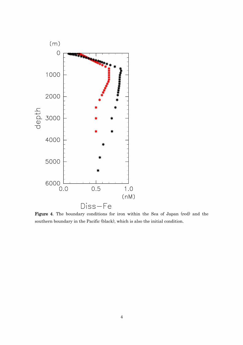
The lateral boundary conditions of iron are shown in Fig. 4, 5, which are 220

11

produced in reference to observational data by Takata et al. (2008) for the Sea of Japan, 221

and Nishioka et al. (2007, 2013) for the Pacific and the results of a simulation by 222

Misumi et al. (2011) for the Bering Sea. In the Sea of Japan and the southern 223

boundary in the Pacific, the boundary concentration data are horizontally constant as 224

shown in Fig. 4. The Misumi et al. (2011)’s data are somewhat revised by reference to 225

the data observed in the Bering Sea by Takata et al. (2005). The boundary conditions of 226

iron are temporally constant. We use the southern boundary iron concentration as the 227

initial condition for the whole model region. 228

In the following sections, the figures are the monthly mean of the 18th year 229

after the coupling the biogeochemical model with the physical model as at least, within 230

the Sea of Okhotsk, the spatial pattern reaches almost an equilibrium. 231

232

3 Sensitivity to parameters in the biogeochemical model 233

3.1 Solubility of dust iron at the sea surface 234

Dust iron solubility at the sea surface is one of the unknown parameters. There 235

are too many factors and processes that control the solubility to determine a proper 236

value for simulations, and not all of those factors and processes have been clarified (e.g. 237

Baker and Croot, 2010). In fact, the dust iron solubility estimates from iron dissolution 238

experiments, using sampled dust, range widely. In the northwestern Pacific, for 239

example, Buck et al. (2006) estimates it as 6±5 %, while Ooki et al. (2009) suggests that 240

it is around 0.4 %. Although Parekh et al. (2005) set it as 1 %, we should examine the 241

sensitivity to it. We conducted experiments with the dust iron solubility of 0 %, 1 %, 5 %, 242

and 10 %. Probably the solubility is not constant over the whole area of the model, as is 243

seen, for example, in the model experiment by Fan et al. (2006). It is, however, assumed 244

12

to be constant both temporally and spatially in the present study. 245

The higher solubility leads to the higher iron concentration because of the 246

increase of total iron input (Figs. 6 and 7). The increase of iron in the intermediate layer 247

is, however, relatively small (Fig. 7), whereas the increase at the sea surface is 248

significant (Fig. 6). These imply that the dust iron is less important for the intermediate 249

layer than the sedimentary iron, at least based on the present model configurations. 250

It is not easy for us to determine which value of solubility is appropriate only 251

from the simulated iron concentration in Figs. 6 and 7 because of the lack of 252

observations, although the iron concentration at the sea surface in the case with the 253

solubility of 10 % is obviously too high compared with the limited observations (not 254

higher than 1.0 nM in the northwestern Pacific; e.g. Nishioka et al., 2007). We, therefore, 255

use the concentration of phosphate to determine the value of iron solubility. 256

The most notable feature in the observed distribution of phosphate in July in 257

the WOA09 (Fig. 8c), when the spring bloom has finished, is a sharp contrast between 258

the Sea of Okhotsk and the Pacific. The concentration is low in the former and high in 259

the latter because phosphate is not completely consumed owing to the deficiency of iron 260

in the Pacific. The contrast also appears in the results of experiments (Fig. 9a-d). 261

However, the concentration in the Pacific becomes significantly lower than the observed 262

values as the solubility of iron increases to 5 % or 10 %. Thus, we consider that 1 %, 263

used by Parekh et al. (2005), is also reasonable in the present model. 264

These experiments also show that the present model is able to represent the 265

HNLC feature caused by iron deficiency in the subarctic Pacific. Phosphate is not 266

depleted in the subarctic Pacific even after the spring bloom, which is a feature of 267

HNLC areas. It decreases as the solubility of iron increases, which indicates that this 268

13

area is deficient in iron when the solubility is low. In contrast, the concentration of 269

phosphate in the Sea of Okhotsk is low in July and changes little even when the 270

solubility of iron increases. This shows that the Sea of Okhotsk in this model is not an 271

HNLC region nor iron-limited region, which is consistent with an observational study 272

by Nakatsuka et al. (2004). 273

274

3.2 Parameters in biological uptake term 275

Although the half saturation constant of Fe, KFe, in eq. (1) is set to be 0.12 nM 276

in the study by Parekh et al. (2005), it may be small for the northwestern Pacific. We set 277

it as 0.5 nM by reference to the study of Noiri et al. (2005). Although the maximum 278

export rate, α, is set to be 0.5 in the study by Parekh et al. (2005), we tuned the value of 279

α, to represent more clearly the difference in the features of an HNLC region; the Pacific 280

in this model region is an HNLC region while the Sea of Okhotsk is not an HNLC 281

region. 282

Figure 10 shows phosphate distribution at the sea surface in July. In the case 283

with the original Parekh’s KFe and α values (KFe=0.12 nM, and α=0.5), phosphate 284

concentration (Fig. 9b) is somewhat smaller in the Pacific and somewhat larger in the 285

Sea of Okhotsk than that in the WOA09 (Fig. 8c). The concentration increases over the 286

entire region when KFe increases to 0.5 nM (Fig. 10a). As α increases (Figs. 10b and 287

10c), the concentration decreases, particularly in the Sea of Okhotsk. Compared with 288

the WOA09, the distribution in Fig. 10c is the most reasonable one: the phosphate is 289

almost depleted in the Sea of Okhotsk and not depleted in the Pacific. Thus, we set KFe 290

and α as 0.5 nM and 1.0, respectively. 291

There is also a need to discuss the dependence of the iron distribution on the 292

14

formulation of scavenging and its parameters, which will be discussed in section 6. 293

294

4 Standard case 295

Using the parameter values determined in section 3, we conducted a 296

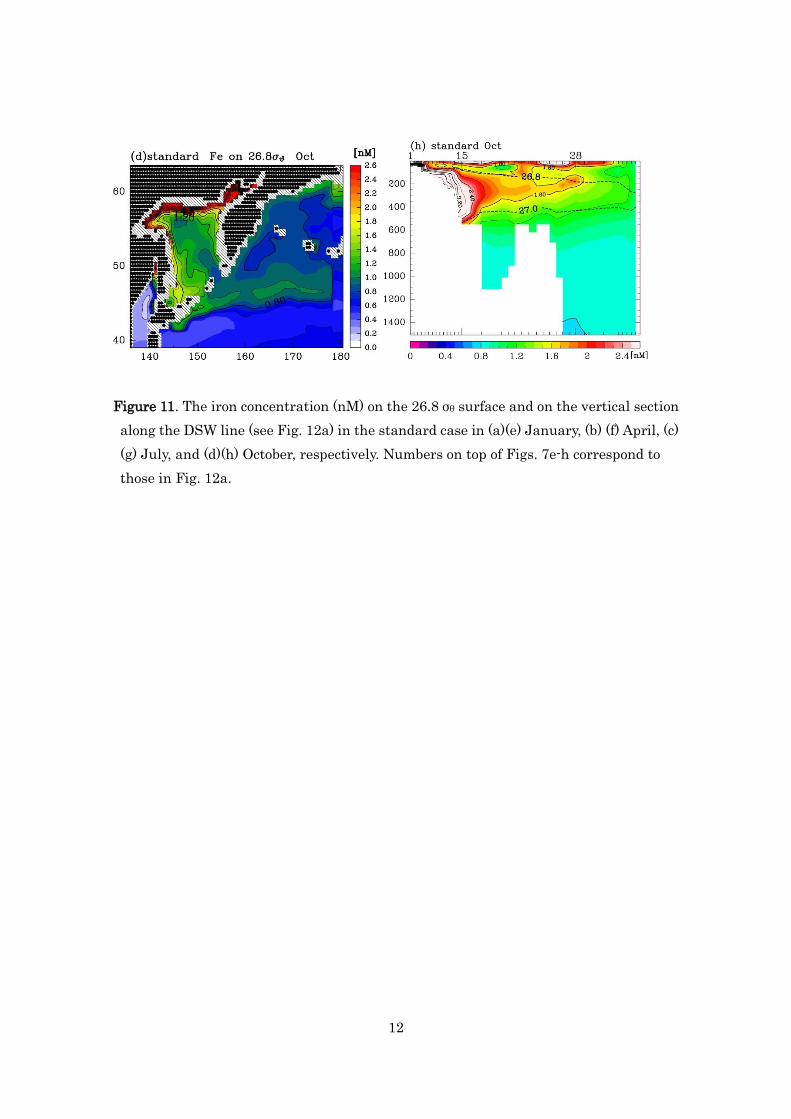
simulation, which we refer to as the standard case. Iron distributions on the 26.8 σθ 297

isopycnal surface in January, April, July, and October are shown in Fig. 11a-d. The high 298

concentration area extends along the northern and the western coasts of the Sea of 299

Okhotsk in all seasons. This suggests that iron is transported from the northern part by 300

the cyclonic circulation, which is the characteristic circulation in a large part of the Sea 301

of Okhotsk (e.g. Ohshima et al., 2004). 302

A high concentration of iron is seen in the intermediate layer, between 26.8 σθ 303

and 27.0 σθ, in the vertical section (Fig. 11e-h) along the red solid line shown in Fig. 12a, 304

which we call the DSW line hereafter. This line is approximately along the path of DSW. 305

Since the core density of DSW in this model is 26.9 σθ (Uchimoto et al., 2011b), the high 306

concentrations extending from the bottom of the shelf in Fig. 11e-h corresponds to DSW. 307

The observational data by Nishioka et al. (2013; 2014) represent very high 308

concentration of iron in the northwestern part of the Sea of Okhotsk, and the maximum 309

of the dissolved iron concentration in the intermediate layer within the Sea of Okhotsk. 310

These features are also seen in the simulated iron concentration in Fig. 11e-h. The 311

simulated data are in good agreement with the observed data shown in Figure 13. The 312

above iron distribution is qualitatively similar to that of chlorofluorocarbons simulated 313

by Uchimoto et al. (2011b). This implies that iron in the intermediate layer is 314

distributed by ocean currents from the northern shelf and the Kuril Straits. 315

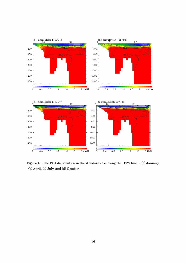
Figure 14 shows the simulated phosphate distribution at the sea surface. 316

15

Although the concentration is somewhat lower than the WOA09 data in Fig. 8, seasonal 317

variations in the Sea of Okhotsk are represented. During summer to early winter the 318

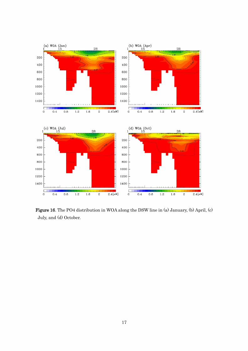
phosphate concentration is low and during late winter and spring, it is high. Figure 15 319

shows the vertical section of phosphate concentration along the DSW line. The 320

concentration of phosphate in the intermediate layer is similar as that of WOA09 (Fig. 321

16), although the simulated concentration near the surface is somewhat lower and that 322

in the deeper layer is somewhat higher than that of WOA09. Figure 17 shows the 323

simulated DOP distribution along the DSW line. In contrast with the phosphate 324

concentration, the DOP concentration in the surface layer is relatively low in January 325

and April (Fig. 17a, b) and high in July and October (Fig. 17 c, d). This is thought to be 326

due to the time scale of the remineralization of DOP. The concentration of DOP in the 327

intermediate layer is low. It is about 0.3 μM in the northwestern shelf area and no more 328

than 0.05 μM in the other areas in Fig. 17. As RFe = 0.47 mmol Fe:mol P, the 329

contribution of the DOP remineralization term to the iron concentration is negligible in 330

the intermediate layer. 331

If sedimentary iron is not given, the high concentration of iron along the path 332

of DSW is not reproduced. Iron concentration is not higher in the western part than the 333

other areas on the 26.8 σθ surface (Fig. 12a), and the iron concentration maximum is not 334

seen in the intermediate layer along the DSW line (Fig. 12b). These results support the 335

hypothesis that the high concentration of iron in DSW primarily originates from the 336

sediments, instead of from aeolian dust. 337

338

5 Potential source region of sedimentary iron 339

As shown above, the sedimentary iron is an important source of iron 340

16

concentration in the intermediate layer of the Sea of Okhotsk. Nakatsuka et al. (2002) 341

reported that a large amount of particles are incorporated into DSW on the 342

northwestern shelf. Iron would be also entrained into DSW there, and thus the 343

northwestern shelf is a likely source region of the sedimentary iron, as is suggested by 344

Nishioka et al. (2007). However it is still an open question whether the northwestern 345

shelf is the only source area for the iron in DSW. We attempt to estimate the relative 346

contribution of shelf regions through sensitivity experiments, although future 347

observations are needed to confirm it. 348

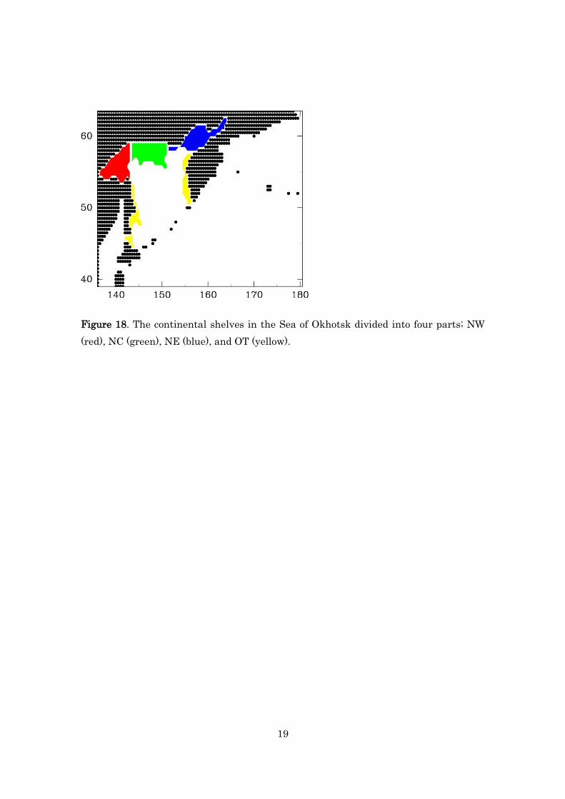
We divided the continental shelf area within the Sea of Okhotsk into four parts 349

almost evenly, as shown in Fig. 18, and changed the sedimentary iron flux in each part. 350

Here, the continental shelf is defined as regions with water depth less than 300 m, and 351

is divided into the northwestern shelf (denoted as NW), the central and eastern parts of 352

the northern shelf (NC and NE, respectively), and the others (OT). OT thus consists of 353

two regions along the eastern and the western boundaries in the Sea of Okhotsk. 354

Several series of numerical experiments (Table 2) were conducted to clarify the 355

contribution of sedimentary iron in each part to iron concentration in the intermediate 356

layer. In a case denoted as AAy, sedimentary iron flux is given in the AA part (e.g. NW) 357

at a rate of y μmol Fe m−2 d−1. For comparison, no sedimentary iron flux is given in 358

NoSed case, and 1 μmol Fe m−2 d−1 is given in all the shelf in the Sea of Okhotsk in 359

ALL1 case. Note that the experiments in the present section were conducted without 360

the sedimentary iron in the Pacific and the dust iron source to clarify the effect of the 361

sedimentary iron within the Sea of Okhotsk. 362

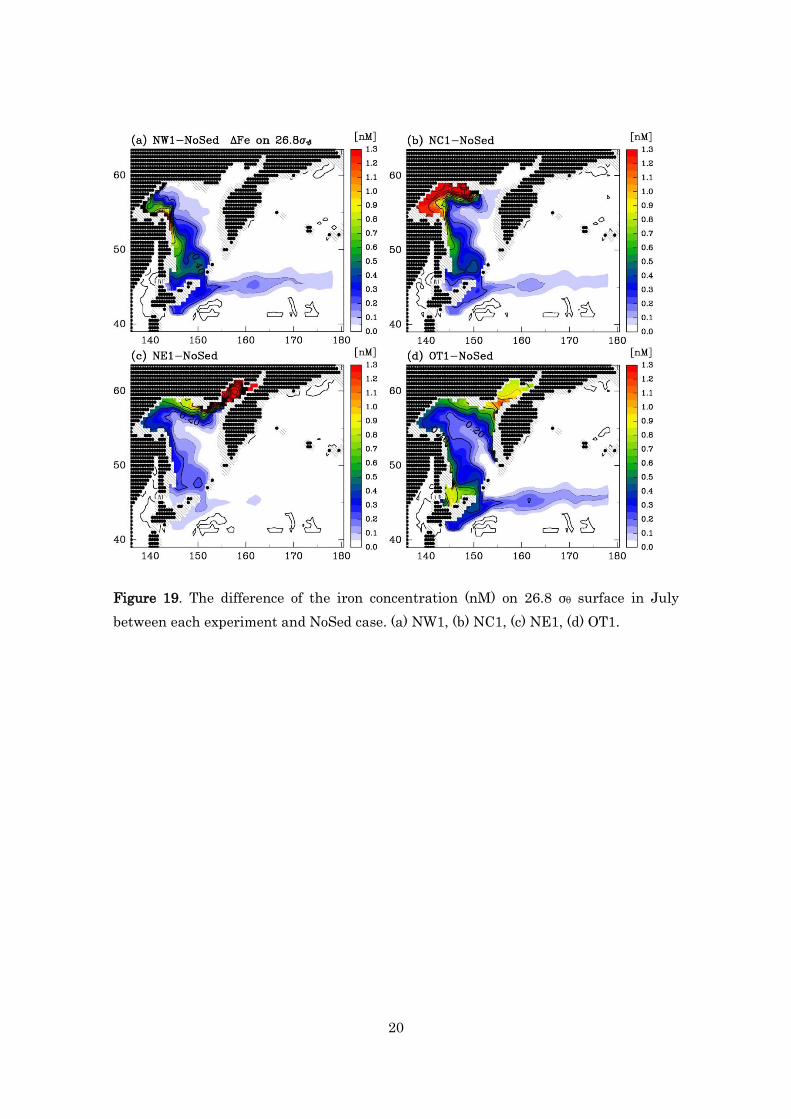
Figure 19 shows the iron concentration of NW1, NC1, NE1 and OT1 cases, 363

after subtraction of that in NoSed case. The figure shows to what extent the 364

17

sedimentary iron from respective sources spreads. The sedimentary iron in each case 365

spreads cyclonically from the source region, with its concentration decreased. In NW1 366

and NC1 cases (Figs. 19a and 19b), the concentration is relatively high off the east coast 367

of Sakhalin (around the path of DSW), but in NE1 case (Fig. 19c) it is low compared 368

with NW1 and NC1 cases. 369

In Fig. 20, iron concentrations in DSW on 50°N are plotted against the 370

sedimentary iron flux (SedFe) given in each part. Here, we define DSW as a watermass 371

with potential temperature less than 1.2°C and with potential density between 26.8 and 372

27.0 σθ, excluding OT area. The iron concentration in DSW increases almost 373

proportionally to SedFe, when SedFe is larger than 1 μmol m-2 d-1 for each part (e.g. 374

NW2-NW10). However, the concentration in the NE cases increases only slightly. This 375

result, as well as Fig. 19c, indicates that sedimentary iron supplied in the eastern part 376

of the northern shelf hardly contributes to the concentration of iron in DSW. Iron in 377

DSW originates mostly from the central and the western part of the northern shelf 378

region, and the path of DSW (i.e. the western part of OT). 379

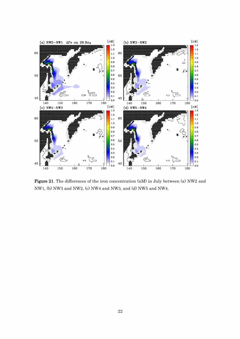
Figure 21 shows the increment of iron concentration on the 26.8 σθ surface 380

when the source flux increases by 1 μmol m-2 d-1 in the NW case, that is, the differences 381

of iron concentration between NW2 and NW1, NW3 and NW2, NW4 and NW3, and, 382

NW5 and NW4. Both the magnitude and spatial extent of the increment are similar 383

when the flux is larger than 3μmol m-2 d-1 (Figs. 21b-d). This is also true in the NC, NE, 384

and OT cases (not shown). The concentration not only in DSW at 50°N (Fig. 20) but the 385

other areas increases nearly proportionally to the flux of iron given at the bottom. 386

Figures 22a and 22b show the differences of iron concentration between 387

NW2O1 and ALL1 cases, and between ALL1 and NW0O1 cases, respectively. The panels 388

18

show an increase of iron concentration resulting from an increase of source iron by 1 389

μmol m-2 d-1 in NW case, but unlike Fig. 21, with an ambient iron concentration coming 390

from sedimentary iron in other areas (NC, NE and OT). These figures are reasonably 391

similar to Figs. 21b-d; particularly Fig. 22a is similar to Fig. 21d, and Fig. 22b is similar 392

to Fig. 21c. Because the areas of NW, NC, NE, and OT regions are roughly the same, the 393

total iron input in NW2O1, ALL1, and NW0O1 is roughly the same as that in NW5, 394

NW4 and NW3, respectively. This suggests that when the total iron input is the same, 395

the increment of iron input in a certain area leads to roughly the same increment in iron 396

concentration. 397

The almost linear increments shown in Figures 20, 21 and 22 are probably 398

associated with the scavenging. As shown in Fig. A1 (c) in the paper by Misumi et al. 399

(2011), scavenging intensity is proportional to total dissolved iron when the total 400

dissolved iron concentration is higher than the total ligand concentration. Physical 401

processes also contribute to the change of iron concentration. In the same current fields, 402

however, their contribution is only the convergence of iron flux, which is also 403

proportional to iron concentration. Thus, iron concentration is thought to increase 404

almost proportionally to iron input. 405

406

6 Discussion 407

In this study, parameters in scavenging formulation are the same as the 408

simulation by Parekh et al. (2005) except for the total ligand concentration. Here, we 409

confirm that the high concentration of iron in the intermediate layer along the DSW line 410

is independent of scavenging parameters, a scavenging scaling factor, τ, and a particle 411

sinking rate, 𝑊sink. We conducted 4 numerical experiments with half and double values 412

19

of τ and 𝑊sink , respectively, of the standard case, where τ is 0.2, and 𝑊sink is 2900 413

m/y. In each experiment, other conditions are the same as in the standard case. The iron 414

concentration increases(decreases) overall when τ becomes small(large) and 𝑊sink 415

becomes large(small) (Fig. 23, 24). However, in all cases, the concentration in the 416

intermediate layer is high. As shown in Fig. 13, the iron concentration in the 417

intermediate layer is consistent with observations in the standard case, and therefore, 418

the values τ = 0.2 and 𝑊sink = 2900 m/y chosen in this study are considered to be 419

reasonable. 420

The simple formulation of scavenging in this model may, however, lead to 421

disagreement of the simulated iron concentration with observational data near the 422

surface and the deep layer as shown in Fig. 13. Although in this formulation, scavenged 423

iron is completely lost, that is, scavenging is a sink of iron, the scavenged iron is 424

actually remineralized within the water column, which is formulated in some models 425

(e.g. Moore and Braucher, 2008). In addition, only the scavenging by particles is 426

considered and that by lithogenic materials (Moore and Braucher, 2008; Galbraith et al., 427

2010) is not considered in our model. These may cause a lower concentration of iron in 428

deep layer than the observation. Higher concentration near the surface in our 429

simulation than the observation may suggest that scavenging there in this model is too 430

weak. Moore and Braucher (2008) increased the scavenging rate near the surface, and 431

Galbraith et al. (2010) changed the ligand stability constant vertically, which results in 432

strong scavenging near the surface. Ye et al. (2011) suggest that colloidal aggregation is 433

an important factor for eliminating dissolved iron. 434

In this model, the influence of sea ice is not sufficiently incorporated as it only 435

includes the attenuation of irradiance and does not include effects of the prevention of 436

20

dust iron entering the sea. In practice, the dust iron is accumulated in the sea ice and 437

transported southward. The supply of the iron from sea ice in its melting season greatly 438

affects the iron concentration in the surface layer in the Sea of Okhotsk (e.g. Kanna et 439

al., 2014). Our model may overestimate the supply of iron at the sea surface covered 440

with sea ice, and underestimate the supply of iron in the surface layer where and when 441

the sea ice melts. However, these might not greatly influence the concentration of iron 442

in the intermediate layer in the present model since the contribution of iron supplied at 443

the sea surface to the intermediate layer is small in this model as shown in Fig. 7. 444

445

7 Concluding remarks 446

We have developed a biogeochemical-physical coupled ocean model to simulate 447

the iron transport and distribution in the Sea of Okhotsk, particularly the high 448

concentration of iron in the intermediate layer, which recent observations have revealed 449

(Nishioka et al., 2007; 2014). The physical part of the model is that of Uchimoto et al. 450

(2011a, b), which well represents the ventilation and the circulation of the intermediate 451

layer in the Sea of Okhotsk. The geochemical part is based on Parekh et al. (2005)’s 452

model, where the iron cycle interacts with the phosphorus cycle but is decoupled 453

through external sources and sink terms. 454

Although the present biogeochemical model is not complex, we have succeeded 455

in reproducing the important features regarding the iron distribution in the Sea of 456

Okhotsk and the northwestern Pacific; such as the high concentration of iron in DSW in 457

the Sea of Okhotsk, the HNLC feature in the northwestern Pacific caused by iron 458

deficiency, and not HNLC in the Sea of Okhotsk. Through the numerical experiments, it 459

was suggested that the high concentration of iron in DSW is attributed mainly to the 460

21

bottom sedimentary iron, not to aeolian dust. However, it should be noted that the 461

present model is not sufficiently complex to be able to represent the detailed iron 462

distribution owing to, for example, ligand distribution, various biological iron uptake 463

processes, and transport of iron by sea ice. There is also uncertainty in the amount of 464

dust iron input and the sedimentary iron input. However, the increase of dust iron input 465

effects a relatively small change in the iron concentration of the intermediate layer in 466

the present model configuration as shown in section 3.1. On the other hand, the 467

sedimentary flux of iron increases the iron concentration of the intermediate layer. 468

Several series of numerical experiments showed that the iron concentration in 469

DSW increases as the sedimentary iron fluxes in the western and eastern part of the 470

northern shelf (NW, NC) and along the DSW (the western part of OT) increase, but that 471

it hardly increases even if the flux in the eastern part of the northern shelf (NE) 472

increases. This implies that the eastern part of the northern shelf is so far from the path 473

of DSW that much of the iron supplied there is scavenged before it reaches the path of 474

DSW in this model configuration. 475

Although the present model reasonably reproduced features of the iron 476

distribution in the Sea of Okhotsk, many important parameters, such as iron dust 477

solubility, remain uncertain and thus they were determined through sensitivity 478

experiments. Recently, iron in the Sea of Okhotsk has attracted attention, and many 479

observations have been and will be conducted, which will help the model improvement. 480

481

acknowledgements 482

We are grateful to N. Mahowald for providing us with the dust dataset. We also thank Y. 483

Hoshiba for his helpful comments on constructing the model. An anonymous reviewer ’s 484

22

thoughtful and constructive comments greatly improved the manuscript. Numerical 485

calculations were performed at the Pan-Okhotsk Information System of Institute of Low 486

Temperature Science, Hokkaido University and the high performance computing 487

system at information initiative center, Hokkaido University. This study was supported 488

by the New Energy and Industrial Technology Development Organization (NEDO), 489

JHPCN and the grant-in-aid for Scientific Research (KAKENHI) No. 222210001 and No. 490

22106010. The figures were produced by GFD-DENNOU Library 491

(http://www.gfd-dennou.org/index.html.en). 492

493

References 494

Archer, D. E., Johnson, K., 2000. A model of the iron cycle in the ocean. Global 495

Biogeochem. Cycles, 14(1), 269–279, doi:10.1029/1999GB900053. 496

497

Baker, A. R., Croot, P. L., 2010. Atmospheric and marine controls on aerosol iron 498

solubility in seawater. Mar. Chem., 120, 4-13. 499

500

Boyle, E. A., Edmond, J. M., 1977. The mechanism of iron removal in estuaries. 501

Geochimica et Cosmochimica Acta, 41, 1313-1324. 502

503

Buck, C. S., Landing, W. M., Resing, J. A., Lebon, G. T., 2006. Aerosol iron and 504

aluminium solubility in the northwest Pacific Ocean: Results from the 2002 IOC cruise. 505

Geochem. Geophys. Geosyst., 7, Q04M07, doi:10.1029/2005GC000977. 506

507

Conkright, M. E., Locarnini, R. A., Garcia, H. E., O’Brien, T. D., Boyer, T. P., Stephens, 508

23

C., Antonov, J. I., 2002. World Ocean Atlas 2001. CD-ROM documentation, 17 pp., Natl. 509

Oceanogr. Data Cent., Silver Spring, Md. 510

511

Cox, M. D., 1987. Isopycnal diffusion in a z-coordinate ocean model. Ocean Modelling 74, 512

1–5. 513

514

Elrod, V. A., Berelson, W. M., Coale, K. H., Johnson, K. S., 2004. The flux of iron from 515

continental shelf sediments: A missing source for global budgets. Geophys. Res. Lett., 31, 516

L12307, doi:10.1029/2004GL020216. 517

518

Fan, S.-M., Moxim, W. J., Levy II, H., 2006. Aeolian input of bioavailable iron to the 519

Ocean. Geophys. Res. Lett., 33, L07602, doi:10.1029/2005GL024852. 520

521

Fukamachi, Y., Mizuta, G., Ohshima, K. I., Talley, L. D., Riser, S. C., Wakatsuchi, M., 522

2004. Transport and modification processes of dense shelf water revealed by longterm 523

moorings off Sakhalin in the Sea of Okhotsk. J. Geophys. Res., 109, C09S10, 524

doi:10.1029/2003JC001906. 525

526

Galbraith, E. D., Gnanadesikan, A., Dunne, J. P., Hiscock, M. R., 2010: Regional 527

impacts of iron-light colimitation in a global biogeochemical model. Biogeosciences, 7, 528

1043-1064. 529

530

Garcia, H. E., Locarnini, R. A., Boyer, T. P., Antonov, J. I., Zweng, M. M., Baranova, O. 531

K., Johnson, D. R., 2010. World Ocean Atlas 2009, Volume 4: Nutrients (phosphate, 532

24

nitrate, silicate). S. Levitus, Ed. NOAA Atlas NESDIS 71, U.S. Government Printing 533

Office, Washington, D.C., 398 pp. 534

535

Gent, P. R., Willebrand, J., McDougall, T. J., McWilliams, J. C., 1995. Parameterizing 536

eddy induced tracer transports in ocean circulation models. J. Phys. Oceanogr., 25, 463–537

474. 538

539

Hasumi, H. 2006. CCSR ocean component model (COCO) version 4.0. CCSR Report 25, 540

103 pp. 541

542

Homoky, W. B., John, S. G., Conway, T. M., Mills, R. A., 2013. Distinct iron isotopic 543

signatures and supply from marine sediment dissolution. Nature Communications, 4, 544

doi:10.1038/ncomms3143. 545

546

Honeyman, B., Balistrieri, L., Murray J., 1988. Oceanic trace metal scavenging and the 547

importance of particle concentration. Deep Sea Res., Part I, 35, 227-246. 548

549

Hunke, E. C. Dukowicz, J. K., 1997. An elastic‐viscous‐plastic model for sea ice 550

dynamics. J. Phys. Oceanogr., 27, 1849–1867. 551

552

Kanna, N., Toyota, T., Nishioka, J., 2014. Iron and macro-nutrient concentrations in sea 553

ice and their impact on the nutritional status of surface waters in the southern Okhotsk 554

Sea. Progress in Oceanography, this issue. 555

556

25

Kitani, K., 1973. An oceanographic study of the Okhotsk Sea: particularly in regard to 557

cold waters. Bulletin of Far Seas Fisheries Research Laboratory, 9, 45-77. 558

559

Mahowald, N., Baker, A., Bergametti, G., Brooks, N., Duce, R., Jickells, T., Kubilay, N., 560

Prospero, J., Tegen, I., 2005. Atmospheric global dust cycle and iron inputs to the ocean. 561

Global Biogeochem. Cycles, 19(4), GB4025, 10.1029/2004GB002402. 562

563

Marchetti, A., Maldonado, M. T., Lane, E. S., Harrison, P. J., 2006. Iron requirements of 564

the pennate diatom Pseudo-nitzschia: Comparison of oceanic (high-nitrate, 565

low-chlorophyll waters) and coastal species. Limnol. Oceanogr., 51(5), 2092-2101. 566

567

Martin, J., Knauer, G., Karl, D., Broenkow, W., 1987. VERTEX: Carbon cycling in the 568

northeast Pacific. Deep Sea Res., 34, 267–285. 569

570

Misumi, K., Tsumune, D., Yoshida, Y., Uchimoto, K., Nakamura, T., Nishioka, J., 571

Mitsudera, H., Bryan, F. O., Lindsay, K., Moore, J. K., Doney, S. C., 2011. Mechanisms 572

controlling dissolved iron distribution in the North Pacific: A model study. J. Geophys. 573

Res., 116, G03005, doi:10.1029/2010JG001541. 574

575

Moore, J. K., Braucher, O., 2008. Sedimentary and mineral dust sources of dissolved 576

iron to the world ocean. Biogeosciences, 5, 631-656. 577

578

Nakamura, T., Awaji, T., 2004. Tidally induced diapycnal mixing in the Kuril Straits 579

and its role in water transformation and transport: A three-dimensional nonhydrostatic 580

26

model experiment. J. Geophys. Res., 109, C09S07, doi:10.1029/2003JC001850. 581

582

Nakamura T., Toyoda, T., Ishikawa, Y., Awaji, T., 2006. Enhanced ventilation in the 583

Okhotsk Sea through tidal mixing at the Kuril Straits. Deep Sea Res. Part I, 53, 584

425-448. 585

586

Nakatsuka, T., Yoshikawa, C., Toda, M., Kawamura, K., Wakatsuchi, M., 2002. An 587

extremely turbid intermediate water in the Sea of Okhotsk: Implication for the 588

transport of particulate organic matter in a seasonally ice-bound sea. Geophys. Res. 589

Lett., 29(16), doi:10.1029/2001GL014029. 590

591

Nakatsuka, T., Fujimune, T., Yoshikawa, C., Noriki, S., Kawamura, K., Fukamachi, Y., 592

Mizuta, G., Wakatsuchi, M., 2004. Biogenic and lithogenic particle fluxes in the western 593

region of the Sea of Okhotsk: Implications for lateral material transport and biological 594

productivity. J. Geophys. Res., 109, C09S13, doi:10.1029/2003JC001908. 595

596

Nihashi, S., Ohshima, K. I., Nakasato, H., 2011. Sea-ice retreat in the Sea of Okhotsk 597

and the ice-ocean albedo feedback effect on it. J. Oceanogr., 67, 551-562, 598

doi:10.1007/s10872-011-0056-x. 599

600

Nishioka, J., Ono, T., Saito, H., Nakatsuka, T., Takeda, S., Yoshimura, T., Suzuki, K., 601

Kuma, K., Nakabayashi, S., Tsumune, D., Mitsudera, H., Johnson, W. K., Tsuda, A., 602

2007. Iron supply to the western subarctic Pacific: Importance of iron export from the 603

Sea of Okhotsk. J. Geophys. Res., 112, C10012, doi:10.1029/2006JC004055. 604

27

605

Nishioka, J., Nakatsuka, T., Watanabe, Y. W., Yasuda, I., Kuma, K., Ogawa, H., Ebuchi, 606

N., Scherbinin, A., Volkov, Y. N., Shiraiwa, T., Wakatsuchi, M., 2013. Intensive mixing 607

along an island chain controls oceanic biogeochemical cycles. Global Biogeochem. Cycles, 608

27, doi:10.1002/gbc.20088. 609

610

Nishioka, J., Nakatsuka, T., Ono, K., Volkov, Y. N., Scherbinin, A., Shiraiwa, T., 2014. 611

Quantitative evaluation of iron transport processes in the Sea of Okhotsk. Progress in 612

Oceanography, this issue. 613

614

Noiri, Y., Kudo, I., Kiyosawa, H., Nishioka, J., Tsuda, A., 2005. Influence of iron and 615

temperature on growth, nutrient utilization ratios and phytoplankton species 616

composition in the western subarctic Pacific Ocean during the SEEDS experiment. 617

Progress in Oceanogr., 64, 149-166, doi:10.1016/j.pocean.2005.02.006. 618

619

Ohshima, K. I., Simizu, D., Itoh, M., Mizuta, G., Fukamachi, Y., Riser, S. C., Wakatsuchi, 620

M., 2004. Sverdrup balance and the cyclonic gyre in the Sea of Okhotsk. J. Phys. 621

Oceanogr., 34, 513-525. 622

623

Ooki, A., Nishioka, J., Ono, T., Noriki, S., 2009. Size dependence of iron solubility of 624

Asian mineral dust particles. J. Geophys. Res., 114, D03202, 625

doi:10.1029/2008JD010804. 626

627

Parekh, P., Follows, M. J., Boyle, E. A., 2005. Decoupling of iron and phosphate in the 628

28

global ocean, Global Biogeochem. Cycles, 19, GB2020, doi:10.1029/2004GB002280. 629

630

Parekh, P., Joos, F., Müller, A., 2008. A modeling assessment of the interplay between 631

aeolian iron fluxes and iron-binding ligands in controlling carbon dioxide fluctuations 632

during Antarctic warm events. Paleoceanography, 23, PA4202, 633

doi:10.1029/2007PA001531. 634

635

Perovich, D. K., 1998. The optical properties of sea ice. Physics of ice-covered seas, vol. 1 636

(ed. M. Leppäranta), 195-230. 637

638

Röske, F., 2001. An atlas of surface fluxes based on the ECMWF re-analysis—A 639

climatological dataset to force global ocean general circulation models. 640

Max-Planck-Institut für Meteorologie Rep. 323, 31 pp. 641

642

Semtner, A. J., Jr., 1976. A model for the thermodynamic growth of sea ice in numerical 643

investigations of climate, J. Phys. Oceanogr., 6, 379–389. 644

645

Shcherbina, A. Y., Talley, L. D., Rudnick, D. L., 2003. Direct observations of North 646

Pacific ventilation: Brine rejection in the Okhotsk Sea, Science, 302, 1952-1955, 647

doi:10.1126/science.1088692. 648

649

Shigemitsu, M., Nishioka, J., Watanabe, Y. W., Yamanaka, Y., Nakatsuka, T., Volkov, Y. 650

N., 2013. Fe/Al ratios of suspended particulate matter from intermediate water in the 651

29

Okhotsk Sea: Implications for long-distance lateral transport of particulate Fe. Mar. 652

Chem., 157, 41-48. 653

654

Takata, H., Kuma, K., Iwade, S., Isoda, Y., Kuroda, H., Senjyu, T., 2005. Comparative 655

vertical distributions of iron in the Japan Sea, the Bering Sea, and the western North 656

Pacific Ocean. J. Geophys. Res., 110, C07004, doi:10.1029/2004JC002783. 657

658

Takata, H., Kuma, K., Isoda, Y., Otosaka, S., Senjyu, T., Minagawa, M., 2008. Iron in the 659

Japan Sea and its implications for the physical processes in deep water. Geophysical 660

Research Letters, 35(2), L02606, doi:10.1029/2007GL031794. 661

662

Tsuda, A., Takeda, S., Saito, H., Nishioka, J., Nojiri, Y., Kudo, I., Kiyosawa, H., 663

Shiomoto, A., Imai, K., Ono, T., Shimamoto, A., Tsumune, D., Yoshimura, T., Aono, T., 664

Hinuma, A., Kinugasa, M., Suzuki, K., Sohrin, Y., Noiri, Y., Tani, H., Deguchi, Y., 665

Tsurushima, N., Ogawa, H., Fukami, K., Kuma, K., Saino, T., 2003. A mesoscale iron 666

enrichment in the western subarctic Pacific induces large centric diatom bloom. Science, 667

300(5621), 958-961. 668

669

Tsuda, A., Takeda, S., Saito, H., Nishioka, J., Kudo, I., Nojiri, Y., Suzuki, K., Uematsu, 670

M., Wells, M. L., Tsumune, D., Yoshimura, T., Aono, T., Aramaki, T., Cochlan, W. P., 671

Hayakawa, M., Imai, K., Isada, T., Iwamoto, Y., Johnson, W. K., Kameyama, S., Kato, S., 672

Kiyosawa, H., Kondo, Y., Levasseur, M., Machida, R. J., Nagao, I., Nakagawa, F., 673

Nakanishi, T., Nakatsuka, S., Narita, A., Noiri, Y., Obata, H., Ogawa, H., Oguma, K., 674

Ono, T., Sakuragi, T., Sasakawa, M., Sato, M., Shimamoto, A., Takata, H., Trick, C. G., 675

30

Watanabe, Y. W., Wong, C. S., Yoshie, N., 2007. Evidence for the grazing hypothesis: 676

grazing reduces phytoplankton responses of the HNLC ecosystem to iron enrichment in 677

the Western Subarctic Pacific (SEEDS II). J. Oceanogr., 63, 983-994. 678

679

Uchimoto, K., Nakamura, T., Mitsudera, H., 2011a. Tracing dense shelf water in the Sea 680

of Okhotsk with an ocean circulation model. Hydro. Res. Lett., 5, 1–5, 681

doi:10.3178/hrl.5.1. 682

683

Uchimoto, K., Nakamura, T., Nishioka, J., Mitsudera, H., Yamamoto-Kawai, M., 684

Misumi, K., Tsumune, D., 2011b. Simulations of chlorofluorocarbons in and around the 685

Sea of Okhotsk: Effects of tidal mixing and brine rejection on the ventilation. J. Geophys. 686

Res., 116, C02034, doi:10.1029/2010JC006487. 687

688

Ye, Y., Wagener, T., Völker, C., Guieu, C., Wolf-Gladrow, D., 2011. Dust deposition: iron 689

source or sink? A case study. Biogeosciences, 8, 2107-2124. 690

31

Figure captions 691

Figure 1. Model domain with geographical names. 692

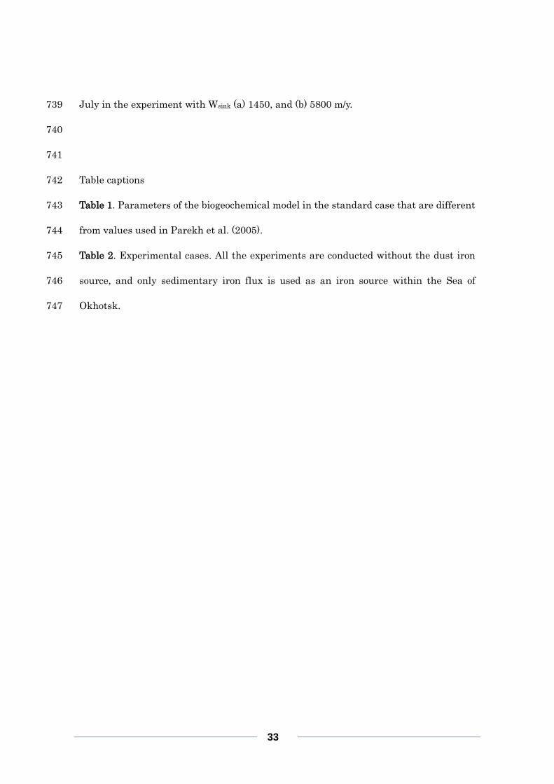
Figure 2. Schematic representation of the phosphorus cycle in the model. 693

Figure 3. Dust deposition distribution (g/m2/y) from Mahowald et al. (2005). 694

Figure 4. The boundary conditions for iron within the Sea of Japan (red) and the 695

southern boundary in the Pacific (black), which is also the initial condition. 696

Figure 5. The boundary condition for iron along the eastern boundary. 697

Figure 6. The iron concentration (nM) at the sea surface in July. The solubility of dust 698

iron is (a) 0, (b) 1, (c) 5, (d) 10 %. 699

Figure 7. The iron concentration (nM) on the 26.8 σθ surface in July. The solubility of 700

dust iron is (a) 0, (b) 1, (c) 5, (d) 10 %. 701

Figure 8. The surface phosphate concentration (μM) of WOA09 in (a) January, (b) April, 702

(c) July, and (d) October. 703

Figure 9. The phosphate concentration (μM) at the sea surface in July in experiments 704

with the dust iron solubility of (a) 0 %, (b) 1 %, (c) 5 %, and (d) 10 %. 705

Figure 10. The phosphate concentration at the sea surface in July. KFe=0.5. (a) α=0.5, (b) 706

α=0.75, (c) α=1.0. 707

Figure 11. The iron concentration (nM) on the 26.8 σθ surface and on the vertical section 708

along the DSW line (see Fig. 12a) in the standard case in (a)(e) January, (b) (f) April, (c) 709

(g) July, and (d)(h) October, respectively. Numbers on top of Figs. 11e-h correspond 710

to those in Fig. 12a. 711

Figure 12. The iron concentration (nM) on the 26.8 σθ surface and on the vertical section 712

along the DSW line in July in the experiment without sedimentary iron source. Red 713

line in (a) shows the DSW line. 714

(a)

(c)

(d)

32

Figure 13. Comparison of modeled (red) and observed (black) iron profile. Observed 715

data were along 52.25°N from 143.5°E to 146°E in August 2006 by Nishioka et al. 716

(2014), and modeled data are along 52.0°N and 52.5°N from 144.5°E to 145.5°E in 717

August and September. 718

Figure 14. The PO4 distribution (μM) from (a) January to (l) December. 719

Figure 15. The PO4 distribution in the standard case along the DSW line in (a) January, 720

(b) April, (c) July, and (d) October. 721

Figure 16. The PO4 distribution in WOA09 along the DSW line in (a) January, (b) April, 722

(c) July, and (d) October. 723

Figure 17. The DOP distribution in the standard case along the DSW line in (a) January, 724

(b) April, (c) July, and (d) October. 725

Figure 18. The continental shelf in the Sea of Okhotsk which was divided into four 726

parts; NW (red), NC (green), NE (blue), and OT (yellow). 727

Figure 19. The difference of the iron concentration (nM) on 26.8 σθ surface in July 728

between each experiment and NoSed case. (a) NW1, (b) NC1, (c) NE1, (d) OT1. 729

Figure 20. The iron concentration in DSW vs. the iron flux in each of the four parts. The 730

cross is no iron source experiment. w: NW, c: NC, e: NE, o:OT 731

Figure 21. The differences of the iron concentration (nM) in July between (a) NW2 and 732

NW1, (b) NW3 and NW2, (c) NW4 and NW3, and (d) NW5 and NW4. 733

Figure 22. The differences of the iron concentration in July between (a) NW2O1 and 734

ALL1, and (b) ALL1 and NW0O1. 735

Figure 23. The iron concentration (nM) on the vertical section along the DSW line in 736

July in the experiment with τ (a) 0.1, and (b) 0.4. 737

Figure 24. The iron concentration (nM) on the vertical section along the DSW line in 738

33

July in the experiment with Wsink (a) 1450, and (b) 5800 m/y. 739

740

741

Table captions 742

Table 1. Parameters of the biogeochemical model in the standard case that are different 743

from values used in Parekh et al. (2005). 744

Table 2. Experimental cases. All the experiments are conducted without the dust iron 745

source, and only sedimentary iron flux is used as an iron source within the Sea of 746

Okhotsk. 747

1

Figure 1. Model domain with geographical name.

2

Figure 2. Schematic representation of the phosphorus cycle in the model.

3

Figure 3. Dust deposition distribution (g/m2/y) from Mahowald et al. (2005).

Mar dust [g/m2 /year] 冊

Feb 同

回

国

崎@咽MM#ヨ噌同

..

Jan 曲

1制"開

I.ongltude

0.0 0，4 0・1.2 1.8 2.0 2." 2.8 3.2

'70 U開2同 1脚

I.ougitude

0.0 0・0・1.2.・ 2.0 2.・2.8 3.2

'7。1加.00 .・0

Lo，，&ltude

。~ U M 1.2 U ~ U U ~

1司

圃圃

.a.

• 司-.戸』

.

"=s

=a‘

• コ.a弘

a》-

-

前

叫

ZM

1t:

i=

e---az-

-u=ー==

同

Z1

1

= -

0

4

0

0

0

.70 1帽1剖 2岨

l.ongltude

。。。叫 0.8 1.2 1.8 1.0 2.4 1.8 3.8

Dec dust [g/m2 /year] 帥

160 18。I.ongltude

0.0 0.' 0・1.2 1.8 2.0 2.‘ 2.8 3.2

.8。

Nov

曲

園

田

岨@咽国

H42喝同

2・o .0。l.ougitude

O.Q 0・0・1.2 1.8 2.0 2.・ a・...

..。..

Oct

国

.8。1順。 2・0L。也~!tude

。.0 0.4 0.8 1.2 1・2.0 2.4 2.・ '.2

1河

4

Figure 4. The boundary conditions for iron within the Sea of Japan (red) and the

southern boundary in the Pacific (black), which is also the initial condition.

5

Figure 5. The boundary condition for iron along the eastern boundary.

6

Figure 6. The iron concentration (nM) at the sea surface in July. The solubility of dust

iron is (a) 0, (b) 1, (c) 5, (d) 10 %.

7

Figure 7. The iron concentration (nM) on the 26.8 σθ surface in July. The solubility of

dust iron is (a) 0, (b) 1, (c) 5, (d) 10 %.

(a)

(c)

(d)

8

Figure 8. The surface phosphate concentration (μM) of WOA09 in (a) January, (b) April,

(c) July, and (d) October.

9

Figure 9. The phosphate concentration (μM) at the sea surface in July in experiments

with the dust iron solubility of (a) 0 %, (b) 1 %, (c) 5 %, and (d) 10 %.

10

Figure 10. The phosphate concentration at the sea surface in July. KFe=0.5. (a) α=0.5, (b)

α=0.75, (c) α=1.0.

11

Figure 11 (continued)

12

Figure 11. The iron concentration (nM) on the 26.8 σθ surface and on the vertical section

along the DSW line (see Fig. 12a) in the standard case in (a)(e) January, (b) (f) April, (c)

(g) July, and (d)(h) October, respectively. Numbers on top of Figs. 7e-h correspond to

those in Fig. 12a.

13

Figure 12. The iron concentration (nM) on the 26.8 σθ surface and on the vertical section

along the DSW line in July in the experiment without sedimentary iron source. Red

line in (a) shows the DSW line.

14

Figure 13. Comparison of modeled (red) and observed (black) iron profile. Observed

data were along 52.25°N from 143.5°E to 146°E in August 2006 by Nishioka et al.

(2014), and modeled data are along 52.0°N and 52.5°N from 144.5°E to 145.5°E in

August and September.

15

Figure 14. The PO4 distribution (μM) from (a) January to (l) December.

16

Figure 15. The PO4 distribution in the standard case along the DSW line in (a) January,

(b) April, (c) July, and (d) October.

17

Figure 16. The PO4 distribution in WOA along the DSW line in (a) January, (b) April, (c)

July, and (d) October.

18

Figure 17. The DOP distribution in the standard case along the DSW line in (a) January,

(b) April, (c) July, and (d) October.

19

Figure 18. The continental shelves in the Sea of Okhotsk divided into four parts; NW

(red), NC (green), NE (blue), and OT (yellow).

20

Figure 19. The difference of the iron concentration (nM) on 26.8 σθ surface in July

between each experiment and NoSed case. (a) NW1, (b) NC1, (c) NE1, (d) OT1.

21

Figure 20. The iron concentration in DSW vs. the iron flux in each part. The cross is no

iron source experiment. w: NW, c: NC, e: NE, o:OT

22

Figure 21. The differences of the iron concentration (nM) in July between (a) NW2 and

NW1, (b) NW3 and NW2, (c) NW4 and NW3, and (d) NW5 and NW4.

23

Figure 22. The differences of the iron concentration in July between (a) NW2O1 and

ALL1, and (b) ALL1 and NW0O1.

24

Figure 23. The iron concentration (nM) on the vertical section along the DSW line in

July in the experiment with τ (a) 0.1, and (b) 0.4.

25

Figure 24. The iron concentration (nM) on the vertical section along the DSW line in

July in the experiment with Wsink (a) 1450, and (b) 5800 m/y.

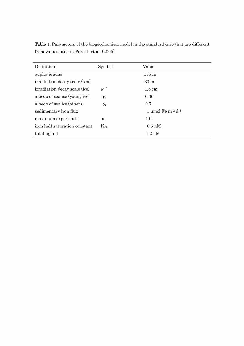
Table 1. Parameters of the biogeochemical model in the standard case that are different

from values used in Parekh et al. (2005).

Definition Symbol Value

euphotic zone 135 m

irradiation decay scale (sea) 30 m

irradiation decay scale (ice) 𝜅−1 1.5 cm

albedo of sea ice (young ice) 𝛾𝐼 0.36

albedo of sea ice (others) 𝛾𝐼 0.7

sedimentary iron flux 1 μmol Fe m−2 d−1

maximum export rate α 1.0

iron half saturation constant KFe 0.5 nM

total ligand 1.2 nM

Table 2. Experimental cases. All the experiments are conducted without the dust iron

source, and only sedimentary iron flux is used as an iron source within the Sea of

Okhotsk.

Case name Sedimentary iron flux

NoSed No sedimentary iron flux

NWx, NCx, NEx, OTx x μmol Fe m−2 d−1 in NW, NC, NE, and OT, respectively

NW2O1 2 μmol Fe m−2 d−1 in NW and 1μmol Fe m−2 d−1 in the others

NW0O1 No flux in NW and 1 μmol Fe m−2 d−1 in the others

ALL1 1 μmol Fe m−2 d−1 in NW, NC, NE, and OT.