Instituto de Engenharia de Sistemas e Computadores de ... · Instituto de Engenharia de Sistemas e...
32
Instituto de Engenharia de Sistemas e Computadores de Coimbra Institute of Systems Engineering and Computers INESC - Coimbra Carla Oliveira Carlos Henggeler Antunes Energy-environment sustainability - a multi-objective approach with uncertain data No. 04 2009 ISSN: 1645-2631 Instituto de Engenharia de Sistemas e Computadores de Coimbra INESC - Coimbra Rua Antero de Quental, 199; 3000-033 Coimbra; Portugal www.inescc.pt
Transcript of Instituto de Engenharia de Sistemas e Computadores de ... · Instituto de Engenharia de Sistemas e...

Instituto de Engenharia de Sistemas e Computadores de Coimbra
Institute of Systems Engineering and Computers
INESC - Coimbra
Carla Oliveira
Carlos Henggeler Antunes
Energy-environment sustainability - a multi-objective approach with uncertain data
No. 04 2009
ISSN: 1645-2631
Instituto de Engenharia de Sistemas e Computadores de Coimbra
INESC - Coimbra
Rua Antero de Quental, 199; 3000-033 Coimbra; Portugal
www.inescc.pt

2
Energy-environment sustainability - a multi-objective approach with uncertain data
Carla Oliveira
INESC Coimbra, Rua Antero de Quental, 199
3030-030 Coimbra, Portugal
Carlos Henggeler Antunes
Dep. Engenharia Electrotécnica e de Computadores, Universidade de Coimbra,
Polo II, 3030-030 Coimbra, Portugal,
INESC Coimbra, Rua Antero de Quental, 199, 3030-030 Coimbra, Portugal
Abstract
Multiple objective programming models allow to consider explicitly distinct axes of
evaluation, generally conflicting and non-commensurable. In particular, multiple
objective linear programming models (MOLP) based on the linear inter/intra industrial
linkages of production can be used to study the interactions between the economy, the
energy system and the environment. This kind of models allows assessing the
environmental impacts, resulting from changes in the level of the economic activities
sustained by distinct policies. However, the uncertainty associated with these model’s
coefficients, namely derived from Input-Output (I-O) analysis, may lead to conclusions
that are not robust regarding the changes of the input data. In this context, we propose a
MOLP model based on I-O analysis with interval coefficients, which allows to assess
impacts on the economy, the energy system and the environment, based on the levels of
activity of economic sectors consistent with distinct policies.
Keywords: MOLP, Input-Output, Economy-Energy-Environment (E3) interactions,
Interval coefficients.
1. Introduction
I-O analysis is an analytical tool, which allows evaluating the inter-relations between
different economic activities being often applied to assess E3 interactions (Hawdon and
Pearson, 1995). I-O analysis and linear programming (LP) are closely related. In its
simplest form, with no substitute inputs, I-O analysis may be regarded as a simple
particular case of LP (Dorfman et al., 1958). The use of the I-O methodology in the
framework of LP models allows obtaining value added information, which would not be
possible to achieve with the separate use of both techniques. Inter/intra-sector relations
embedded in I-O analysis allow designing the production possibility frontier. LP models
allow choosing the optimum level of activities, which cope with a certain objective,
respecting the productive relations imposed by I-O analysis.
3
Traditional studies, which use I-O analysis in the framework of LP, generally consider a
single objective function to be maximized or minimized, usually an aggregated economic
indicator. However, most real-world problems inherently incorporate multiple,
conflicting and incommensurable axes of evaluation of the merit of potential solutions. In
this context, mathematical programming models for decision support become more
representative of reality if distinct aspects of evaluation are explicitly brought into
consideration.
Generally, in most real-world situations, the necessary information to specify the exact
model’s coefficients is not available, because data is scarce, difficult to obtain, uncertain
and the system being modelled may be subject to changes. Therefore, mathematical
programming models for decision support must take explicitly into account, besides
multiple and conflicting objective functions, the treatment of the uncertainty associated
with the model coefficients.
Interval programming is one of the approaches to tackle uncertainty in mathematical
programming models, which possesses some interesting characteristics, since it does not
require the specification of the probabilistic distributions (as in stochastic programming)
or the possibilistic distributions (as in fuzzy programming) of the model coefficients
(Oliveira and Antunes, 2007). Interval programming just assumes that information about
the range of variation of some (or all) of the coefficients is available, which allows to
specify an interval mathematical programming model.
In this paper, we propose a MOLP model based on I-O analysis with interval coefficients
to study E3 interactions. The model herein proposed is aimed at providing the decision-
maker (DM) with information about robust solutions, that is, solutions with good
performance for different model coefficient settings. In the next sections, a detailed
description of the model is given. Finally, some illustrative results obtained using an
algorithm developed to provide decision support in MOLP problems with interval
coefficients are analysed.
2. The model
In what regards to previous studies (see Oliveira and Antunes (2004), Antunes et al.
(2002)) the model incorporates:
• recent changes in the System of National Accounts consistent with the European
System of Accounts (ESA95);
• 80 (real and artificial) activity branches;
• volume and price components of the economy;
• interval coefficients for the energy use within the I-O coefficients matrix (as well as in
other constraints);
• emissions not only from the combustion processes but also from other sources;
• the acidification equivalent potential (AEP) and the tropospheric ozone potential
(TOP), besides the global warming potential (GWP).
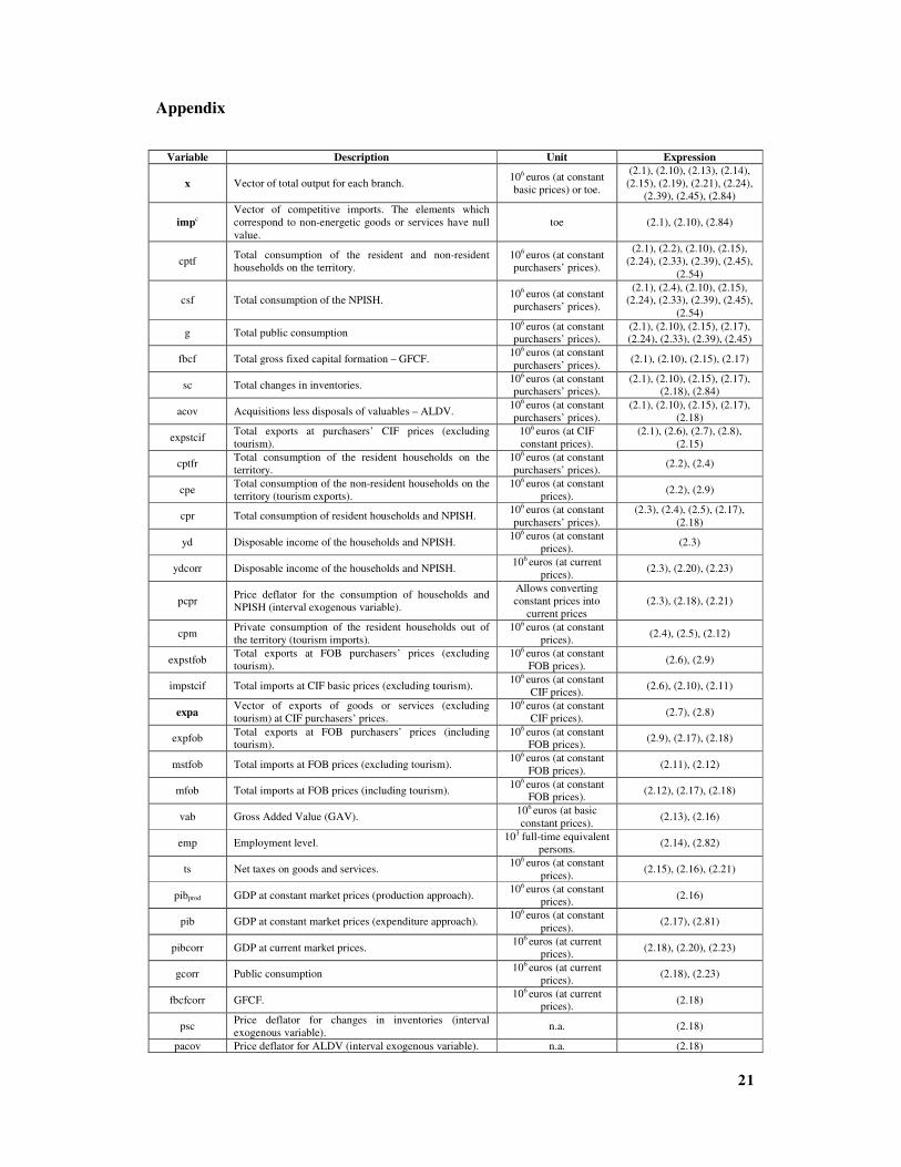
The main model variables are the production of the activity sectors, the Gross Added
Value (GAV), the level of employment, imports and exports, the private consumption,
GDP, the public administrations’ global balance, the public debt, the GWP, the AEP and
the TOP. The detailed description of the variables and coefficients of the model is given
in appendix.

4
2.1. Constraints
The intermediate consumption and final demand of goods or services of each activity
sector shall not exceed the total amount available from national production and
competitive imports of that same good or service:
Ax + acptf (cptf)+ acsf (csf)+ ag (g) + afbcf (fbcf) + asc (sc) + aacov (acov) + aexp (expstcif) ≤
x + impc, (2.1)
cptf ≤ cptf*, csfL ≤ csf ≤ csf
U, g
L ≤ g ≤ g
U, fbcf
L ≤ fbcf ≤ fbcf
U, sc
L ≤ sc ≤ sc
U, acov
L ≤
acov ≤ acovU, expstcif ≥ expstcif
L.
The households’ consumption on the territory corresponds to the consumption of the
resident households plus the consumption of the non-resident households on the territory:
cptf = cptfr + cpe, (2.2)
cpe ≤ cpe*.
The residents’ (households and non-profit institutions serving households - NPISH)
consumption is considered linearly dependent on the disposable income of the residents
at constant prices (deflated by the price index for consumption):
cpr = β0 + β1 (yd = pcpr
ydcorr), (2.3)
cpr ≤ cpr*, yd ≤ yd*.
The households’ consumption on the territory is obtained after deducting from the
residents’s consumption the tourism imports and the consumption of the NPISH:
cptfr = cpr - cpm - csf, (2.4)
cptfr ≤ cptfr*, cpm ≤ cpm*.
The tourism imports are considered as a fixed proportion (exogenously defined) of the
residents’ consumption:
cpm = (α) (cpr). (2.5)
Total exports at constant FOB (free on board) prices are obtained after deducting the
CIF/FOB adjustment to the value of total exports at CIF (cost insurance and freight)
prices:
expstfob = expstcif – (aciffob) (impstcif), (2.6)
expstfob ≤ expstfob*,
impstcif ≥ impstcifL.
Exports at constant purchasers’ prices are obtained by adding to the exports at constant
basic prices the corresponding net taxes:
expa = aexp (expstcif) p̂ exp + aexpts (expstcif). (2.7)
Total exports (excluding tourism) correspond to:
expstcif = e1T expa. (2.8)
Total exports (including tourism) are obtained from (2.6) by adding the tourism exports:
expfob = expstfob + cpe, (2.9)

5
expfob ≤ expfob*.
Total imports are obtained by adding the imports of non-energetic goods and services to
the (competitive and non-competitive) imports of energy in monetary units:
impstcif = (pimpc)T imp
c + (pimpnc)
T (Am
ncx + asc
nc sc) + e2
TAmx + e3
T amcptf (cptf) + e4
T
amcsf (csf) + e5T amg (g) + e6
T amfbcf (fbcf) + e7
T amsc (sc) +
e8T amacov (acov), (2.10)
Total imports at FOB constant prices are obtained by deducting the CIF/FOB adjustment
to the total imports at CIF constant prices:
mstfob = impstcif (1 - aciffob), (2.11)
mstfob ≤ mstfob*.
Total imports (including tourism) are obtained from adding (2.11) to (2.5):
mfob = mstfob + cpm, (2.12)
mfob ≤ mfob*.
The GAV for each activity branch is obtained by multiplying the corresponding output by
a product’s transformation coefficient.
vab = aremT x + aot
T x - aos
T x + aebermb
T x. (2.13)
The employment level for each activity branch is obtained after dividing the output by the
corresponding expected labour gross productivity for each branch.
emp = lT x. (2.14)
Net taxes on products are computed by using net tax coefficients both on the intermediate
consumption and on final demand flows:
ts = e9T
Ats x + e10T
acptfts (cptf) + e11T acsfts (csf) + e12
T agts (g) + e13
T afbcfts (fbcf) + e14
T ascts
(sc) + e15T aacovts (acov) + e16
T aexts (expstcif) +
+ e17T Ats
nc x, (2.15)
ts ≥ tsL.
GDP can be computed according to three distinct perspectives: income approach,
production approach and expenditure approach. The first two approaches are similar and
only the last two are herein considered, since the intrinsic coherence of the model does
not guarantee that these two definitions lead to the same results. However, the use of
interval coefficients leads to different results in these two approaches. Hence, we have
considered that the lower bound of GDP according to the production approach should
never exceed the upper bound according to the expenditure approach, assuming that there
might be a slight deviation between the interval values obtained with both approaches.
pibprod = vab + ts, (2.16)
pibL ≤ pibprod ≤ pib*.
pib = cpr + g + fbcf + sc + acov + expfob – mfob, (2.17)
pibL ≤ pib ≤ pib*.
The GDP at current prices is obtained from the distinct components of GDP at constant
prices according to the expenditure approach, which are multiplied by the corresponding
deflators:
pibcorr = (cpr) (pcpr) + gcorr + fbcfcorr + (sc) (psc) + (acov) (pacov) + (expfob)
(pexpfob) – (mfob) (pmfob), (2.18)

6
pibcorr ≤ pibcorr*, gcorrL ≤ gcorr ≤ gcorr
U, fbcfcorr
L ≤ fbcfcorr ≤ fbcfcorr
U.
The wages and salaries can be evaluated in real terms by deflating them with an index
which reflects the prices of the products purchased.
remcorr = aremT x (iucl), (2.19)
remcorr ≤ remcorr*.
The disposable income of households and NPISH equals the difference between the
National Available Income and the sum of the available income of corporations and
public administration. The available income of the corporations (savings) represents a
given (exogenous) fixed proportion of GDP.
ydcorr = pibcorr (1 - pspibcorr) + (rp+ - rp
- + tisub - (tisub) tigts) + tre - (rtdydcorr)
ydcorr - (tdscpibcorr) (pibcorr) - (tcss) (remcorr) - tisub - (repgpibcorr) (pibcorr)
+ trig , (2.20)
ydcorr ≤ ydcorr*, rp+ - rp
- ≤ rp*, tisub ≤ tisub*, (tisub) tigts ≤ tisubg*, tre ≤ tre*,
(rtdydcorr) ydcorr ≤ td*, (tdscpibcorr) (pibcorr) ≤ tdsc*, (tcss) (remcorr) ≤ css*,
(repgpibcorr) (pibcorr) ≤ repg*, trig ≤ trig*.
Net indirect taxes at current prices are computed by using the price deflator for the
consumption of households and NPISH and an index for the evolution of the indirect
fiscal burden:
tisub = (aot x – aos x + ts) (pcpr) (itis). (2.21)
Public debt results from accumulating the previous period debt with the symmetric value
of the public administrations’ global balance, plus one adjustment variable, which in turn
results from the variation of the debts assumed by the Treasury, net of the privatization
revenues.
div = div-1 – (sgg+ - sgg
-) + dat, (2.22)
div ≤ div*, div-1 ≥ div-1*, (sgg+ - sgg
-) ≥ sgg*, dat ≥ dat*.
Public administration’s global balance is obtained after subtracting to the public
administration’s revenues the public administration’s expenditures:
(sgg+ - sgg
-) = (rtdydcorr) ydcorr + (tdscpibcorr) (pibcorr) + (tcss) (remcorr) + (tisub)
(tigts) + (repgpibcorr) (pibcorr) - gcorr - trig + treg - rg (div-1 + div)/2 + (tkpibcorr)
(pibcorr) + trkg – gfbcf, (2.23)
treg ≤ treg*, rg (div-1 + div)/2 ≤ jurg*, (tkpibcorr) (pibcorr) ≤ tk*, trkg ≤ trkg*, gfbcf ≥
gfbcf*.
In the I-O table, the total fuel use is the total amount of fuel production plus imports.
Nevertheless, the energy use for exports and investment shall not be taken into account in
the emission computations (Proops et al., 1993).
ecco2E = Eˆtjcf E
ˆcef Eˆocf [AEx + acptfE cptf + acsfE csf + agE g – NEx + ancptfE (cptf) +
ancsfE (csf) + angE (g)] (1244 ) (10
-3). (2.24)
Total CO2 emissions from fuel combustion are obtained by summing up all the elements
in (2.24):
ecco2 = T18e ecco2E. (2.25)
The emission factors used in the computation of other pollutant emissions (CO, NOx,
N2O, CH4, NMVOC, NH3 and SO2) are highly dependent on the technology used. From

7
this point onwards the pollutants emitted are designated by the letter w, where
w = 1 = CO, 2 = NOx, 3 = N2O, 4 = CH4, 5= NMVOC, 6 = SO2, 7 = NH3, 8 = CO2.
Combustion emissions from electricity generation and co-generation are computed by
considering that non-energetic oil products have null emission factors.
ecelectw = (fecelectw)T ( Etjcfˆ (AEelect xelect)) (10
-9). (2.26)
eccogw = (feccogw)T ( Etjcfˆ (AE.cog xcog)) (10
-9). (2.27)
In the computation of combustion emissions from refining activities, only the energetic
oil for the refineries’ own use is taken into account.
ecrefw = (fecrefw)T ( Etjcfˆ (AE.ref - NE.ref) xref)) (10
-9). (2.28)
Combustion emissions from the industrial and construction branches should be net of the
use of oil products for non-energetic purposes.
ecindw = (fecindw)T ( Etjcfˆ (AEind - NEind)xind) (10
-9). (2.29)
The computation of combustion emissions in the transportation branches is based on the
IPCC (1996a, 1996b, 1996c, 2006) emission factors.
ectrtw = (fectrtw)T ( Etjcfˆ (AE.t xt)) (10
-9), (2.30)
where t = 60, 61, 62 are activity branches of the I-O matrix.
Sulphur dioxide emissions are directly linked to the sulphur content of the fuels.
fectrctw = (2 ) (s) (q
1) (10
9) (1 - r) (1 - tred). (2.31)
In the computation of combustion emissions from the agriculture and services branches,
the non-energetic oil products have null emission factors.
ecosyw = (fecosyw)T ( Etjcfˆ (AE.y xy)) (10
-9), (2.32)
where y = 1 = agriculture and catle 2 = forests, 5 = fishing, 41 = water capturing and
distribution, 50 to 55 and 63 to 93 = services.
Combustion emissions from final consumption have null emission factors for non-
energetic oil products.
eccpw = (feccpw)T ( Etjcfˆ [(acptfE cptf) + (acfsE csf) + (agE g)] (10
-9). (2.33)
Total emissions of other pollutants from fuel combustion are obtained by summing up
(2.26) to (2.30) and (2.32) to (2.33):
ecw = ecelectw + eccogw + ecrefw + ecindw + ∑t
wtectr + ∑y
wyecos + eccpw, (2.34)
Indexes t and y have the range of variation referred from (2.30) to (2.32).
Fugitive emissions obtained from the transportation of crude oil are computed
considering as activity the crude oil consumption in the refining sector.
eftpbw = (apbref xref ) (fctpb) (feftpbw) (10-9
). (2.35)
In the computation of the fugitive emissions from refining activities, the activity
considered is the output of the refining sector.
efppw = (xref ) (fefppw) (10-9
). (2.36)

8
According to the National Inventory Emissions Report (Ferreira et al., 2006), the activity
considered for computing fugitive emissions is the national output of gasoline refined
both for domestic and foreign markets.
efdistw = (xgasolina) (fctgasolina)(fefdistw) (10-9
). (2.37)
The emissions from vehicle supply of gasoline should only include the ones resulting
from vehicle supply and eventual losses of gasoline. However, since the imported
gasoline can also be exported we have considered the same activity of (2.37) for the
emission computations.
efabastw = (xgasolina) (fctgasolina) (fefabastw) (10-9
). (2.38)
The activity considered for the computation of fugitive emissions from natural gas
transmission is the amount of natural gas transmitted/distributed.
efgnw = (AEgn. x + acptfgn cptf + acsfgn csf + aggn g) (fctjgn) (fefgnw) (10-9
). (2.39)
The activity considered for venting and flaring in the refining sector is the output level of
this activity branch.
efventw = (feventw) (xref ) (10-9
). (2.40)
The activity considered for computing fugitive emissions from geothermal energy is the
amount of geothermal energy produced.
efgeotw = (fegeotw) (fctjgeot) (xgeot) (10
-9). (2.41)
Total fugitive emissions are obtained by summing up (2.35) to (2.41):
efw = eftpbw + efppw + efdistw+ efabastw + efgnw+ efventw + efgeotw. (2.42)
The activity considered for computing emissions from industrial processes is the output
level of the activity sectors.
eprjw = (feprjw) (xj) (10-9
). (2.43)
Total emissions from industrial processes are obtained by summing up the emissions of
pollutant w in the different activity branches:
eprw =∑j
jwepr . (2.44)
Emissions referring to the use solvents (non-energetic oil) are obtained in the following
way:
efsolvw = (AEsolv. x + acptfsolv cptf + acsfsolv csf + agsolv g) (fctsolv) (fefsolvw)
(10-9
). (2.45)
Emissions regarding other products use (paint application and others) are computed
according to the output levels of the activity sectors which use them.
efoutjw = (fefoutjw) (xj) (10-9
). (2.46)
Total emissions from solvent and other products use are obtained by summing up the
emissions of pollutant w in the different activity branches:
efsolvoutw = efsolvw + ∑j
wjefout . (2.47)
The computation of emissions (where w = 1, 2, 3, 5, 6 and the components of the
constraints only assume non-null values for w = 3) from manure management takes into
account the system of animal waste management used:

9
egterw = (aestr) (apecr xy) (agtegr)T (fegtewg) (10
-3), (2.48)
where r = 1 = dairy cattle, 2 = non-dairy cattle, 3 = swine for reproduction, 4 = swine, 5 =
poultry, 6 = other poultry, 7 = sheep, 8 = goats, 9 = horses, 10 = mules and asses, 12 =
rabbits for reproduction, g = 1 = anearobic lagoon, 2 = liquid system, 3 = solid storage, 4
= pasture range padock and y = 1.
The computation of NH3 and CH4 emissions (where w = 4, 7) from manure management
corresponds to:
egterw = (fegterw) (apecr xy) (10-3
). (2.49)
The computation of CH4 emissions from enteric fermentation is obtained from (where the
elements of the constraints have only non-null values for w = 4):
efentrw = (fefentrw) (apecr xy) (10-3
). (2.50)
In order to obtain the NMVOC emissions from the burning of agriculture residues, the
emission factors are multiplied by the total amount of agricultural residues; for the other
emissions, only the dry matter fraction of agricultural residues must be taken into account.
eqraaw = (araa) (fsecaa) (apaa xy) (aqraa) (feqraaw) (10-9
), (2.51)
where a = 1 = vineyard; 2 = orchards and fresh products, 3 = olive orchards, 4 = rice.
The emissions from the use of nitrogen fertilizers are directly linked to the application
pattern of nitrogen fertilizers, according to the total cultivated area.
efndw = (fefndw) (afnd) ( ∑=
4
1aya xapa ) (10
-9). (2.52)
where d = 1 = direct deposition, 2 = atmospheric deposition, 3 = nitrogen leaching.
Total emissions from agriculture are obtained from expressions (2.48) to (2.52).
eagricw = ∑r
wregte + ∑r
rwefent + ∑a
waeqra +∑d
wdefn . (2.53)
Indexes r, a and d have the range of variation referred from (2.48) to (2.52).
Municipal solid wastes (MSW) are produced, in general, by the households and by the
commerce and services sectors.
rsu = (arsudom) (cptf + csf) + (arsucomserv) e19T
(xcomserv) + (arsu90) (xy). (2.54)
The amount of MSW, which goes to solid waste disposal sites (SWDS) is computed
according to a fixed proportion defined exogenously:
rsuaterrou = (rsu) (frsuaterro)(aresiduou). (2.55)
where u = 1 = organic waste , 2 = paper and card, 3 = plastic, 4 = wood, 5 = glass, 6 =
metals, 7 = textiles, 8 = other inerts.
Within constant conditions, the rate of CH4 generation depends on the carbon content of
the waste being disposed. NH3 emissions are computed by replacing the CH4 generation
potential by the corresponding generation potential of NH3 (Instituto do Ambiente et al.,
2004).
ersuaterrouw = ∑n
[(1 – uk−e ) (rsuaterroun) (mfcrsuu) (docrsuu) (docfrsuu) (fw) (
1216 )
(1 – n)2010(ku −−
e )](10-3
), (2.56)
where w = 1, 2, 3, 5, 6, 7 and the components of the constraints only assume non-null
values for w = 4, 7 and u = 1, …, 8.

10
NMVOC emissions are computed using the amount of CH4 emissions generated from
SWDS and the concentration of non-methane organic compounds. No co-deposition was
considered for 2010.
ersuaterrouw = [(2) (ersuaterro4u/densch4) (106) (cconm) (10
-6) (
top)273)(1000)(10)(205.8(
p)(86.18)(po5 +− )]
(covnm) (10-6
). (2.57)
Since there is no data available about the amount of waste of each type assigned to
anaerobic digestion, an exogenous fraction is defined for this system of waste treatment.
ersucompw = (rsu) (frsucomp) (fersucompw) (1 - redemrsuw) (10-6
). (2.58)
Only non-hazardous industrial waste is accounted for (see Insituto do Ambiente et al.
(2004)). In what concerns to NH3 emissions we have applied a proportionality factor
between these emissions and CH4 (similarly to Instituto do Ambiente et al. (2004)).
eriborgaterrow = (feriborgw) [( ∑j
jj fripri) - (1 )(x )(ari ) (fribaterro) (friborgaterro)]
(10-6
), (2.59)
where w = 1, 2, 3, 4, 6, 7, 8 and the components of the constraints only assume non-null
values for w = 4, 7 and j = 15 to 37 (activity branches of the I-O matrix).
NMVOC emissions from industrial organic waste deposition on SWDS are computed
analogously to (2.57).
eriborgaterrow = [(2)(eriborgaterro4/densch4)(106)(cconm)(10
-6) (
top)273)(1000)(10)(205.8(
p)(86.18)(po5 +− )]
(covnm) (10-6
), (2.60)
where w = 5.
We have only considered the non-hazardous industrial waste incineration without
energetic use, since its combustion with energetic purpose has already been considered in
the electricity and co-generation combustion emissions.
eribincinw = [(∑j
jj fripri) - (1 )(x )(ari ) (fribincinsve)] (feribincinw) (10-6
). (2.61)
Emissions regarding the incineration of hospital waste are computed according to the
total amount of hospital waste incinerated per unit of output of activity branch 85 (health
services).
erhincinw = (arhincin85) (xy) (ferhincinw) (10-6
), (2.62)
where y = 85 and each constraint component has a null value for w = 8.
The computation of CO2 emissions regarding waste incineration should only refer to the
amount of non-biogenic waste incinerated, having mainly into account the carbon content
of the waste (e.g. plastics and synthetic textiles).
eresincinw = [((rsu)(frsuincin) + (∑j
jj fripri) - (1 )(x )(ari ) (fribincin)) (ccrsurib) (fcfrsurib)
+ (arhincin85) (xy) (ccrh) (fcfrh)] (1244 ) (efqueima) (10
-3), (2.63)
where each constraint component has non-null values only for w = 8.
Total emissions from waste management are obtained from (2.54) to (2.65)
11
eresw = ∑u
wuersuaterro + ersucompw + eriborgaterrow + eribincinw +
+ erhincinw + eresincinw. (2.64)
Index u varies in the range referred in (2.55).
The computation of the degradable organic component (DOC) in domestic waste water is
based on the per capita biochemical oxygen demand.
tow = (p) (bod). (2.65)
In order to compute the emissions of CH4 regarding domestic waste water handling, an
emission factor per unit of DOC is applied (Ferreira et al., 2006).
eagddsw = (feagd1w) (tow – (ds) (tow)) (1 – recagdtw) + (fesdw) (ds) (tow) (1 – recdsw)
(10-6
), (2.66)
where w = 1, 2, 4, 6 and each component has only non-null values for w = 4.
The computation of NH3 and N2O emissions regarding domestic waste water handling is
based on the application of an emission factor per unit of Nitrogen (N) (Instituto do
Ambiente et. al, 2004).
eagddsw = (feagd2w) (p) (cprot) (fnpr) (fsepticas) (10-6
), (2.67)
where w = 3, 7.
NMVOC emissions regarding domestic waste water handling are computed through the
application of an emission factor per volume of waste water handled.
eagddsw = (feagd3w) (p) (cagd) (fsaneamento) (10-6
), (2.68)
where w = 5.
The computation of N2O, CH4 and NMVOC emissions from industrial waste water
handling is based on a DOC value constant between 1993 and 2000, and assumed to be
33 000 in thousands of inhabitants equivalent until 2010 (see Instituto do Ambiente et al.
(2004)).
eagindw = (dcind) (feagindw) (10-6
), (2.69)
where each element assumes non-null values only for w = 3, 4, 5.
Total emissions of CO
etco = ecw + efw + eprw + efsolvoutw + eagricw+ eresw + eagddsw +
+ eagindw, (2.70)
etco ≤ etcoU,
where w = 1.
Total emissions of NOx
etnox = ecw + efw + eprw + efsolvoutw + eagricw+ eresw + eagddsw +
+ eagindw (2.71)
etnox ≤ etnoxU,
where w = 2.
Total emissions of N2O
etn2o = ecw + efw + eprw + efsolvoutw + eagricw+ eresw + eagddsw +
+ eagindw, (2.72)

12
etn2o ≤ etn2oU,
where w = 3.
Total emissions of CH4
etch4 = ecw + efw + eprw + efsolvoutw + eagricw+ eresw + eagddsw +
+ eagindw, (2.73)
etch4 ≤ etch4U,
where w = 4.
Total emissions of NMVOC
etcovnm = ecw + efw + eprw + efsolvoutw + eagricw+ eresw + eagddsw +
+ eagindw, (2.74)
etcovnm ≤ etcovnmU,
where w = 5.
Total emissions of SO2
etso2 = ecw + efw + eprw + efsolvoutw + eagricw+ eresw + eagddsw +
+ eagindw, (2.75)
etso2 ≤ etso2U,
where w = 6.
Total emissions of NH3
etnh3 = ecw + efw + eprw + efsolvoutw + eagricw+ eresw + eagddsw +
+ eagindw, (2.76)
etnh3 ≤ etnh3U,
where w = 7.
Total emissions of CO2
etco2 = ecco2 + efw + eprw + efsolvoutw + eresw, (2.77)
etco2 ≤ etco2U,
where w = 8.
The most relevant gases leading to GHG emissions (CO2, CH4 e N2O) and excluding land
use changes, are obtained in the following way (Instituto do Ambiente, 2005):
pag = etco2 + (310) (etn2o) + (21) (etch4), (2.78)
pag ≤ pagU.
SO2, NOx and NH3 emissions are aggregated in an “equivalent acid” indicator after
assigning each specific pollutant to a certain weight factor (Instituto do Ambiente, 2005):
eac = (21.74) etnox + (31.25) etso2 + (58.82) etnh3, (2.79)
eac ≤ eacU.
The tropospheric ozone is an indicator which allows the aggregation of NOx, NMVOC,
CO and CH4 emissions after assigning to each one of them a specific weight factor, being
measured in NMVOC equivalent (Instituto do Ambiente, 2005).
pfot = (1.22) (etnox) + etcovnm + (0.11)(etco) + (0.014) (etch4), (2.80)
pfot ≤ pfotU.
13
2.2. Objective functions
The allocation of energetic resources should be made having in mind that the energy
sector is a part of the economic system as a whole and that energy planning requires the
incorporation of economic, social, energetic and environmental objectives. In this way,
the model herein proposed considers the following objective functions.
GDP can be seen as a measure of the economic performance to be maximized:
max Z1 = pib. (2.81)
The total level of employment in the economy might be faced as a measure of social
well-being to be maximized:
max Z2 = emp. (2.82)
The minimization of the impact of economic activities in the GWP, measured through the
emission of GHG, leads to the consideration of the following objective function:
min Z3 = pag. (2.83)
Since the country presents a strong foreighn energy dependency, the minimization of
energy imports has been considered:
min Z4 = (e20)T imp
c + (e21)
T (Am
ncx + asc
nc sc). (2.84)
3. The interactive method
The interactive approach used to obtain compromise solutions to the MOLP model based
on I-O analysis with interval coefficients herein suggested is based on Oliveira and
Antunes (2009).
Let the MOLP problem with interval coefficients be given, without loss of generality, by:
max Zk(x) = [ ]∑=
n
1j
jUkj
Lkj x, cc , k = 1, …, p,
s.t. [ ]∑=
n
1j
jUij
Lij x, aa ≤ [ ]U
iLi , bb , i = 1, …, m,
xj ≥ 0, j = 1, …, n, (2.85)
where [ ]Ukj
Lkj , cc , [ ]U
ijLij , aa and [ ]U
iLi , bb , k = 1, …, p, j = 1, …, n and i = 1, …, m, are
closed intervals.
The method starts by obtaining two surrogate deterministic problems, by considering the
minimization of the worst possible deviation of the interval objective functions from their
corresponding interval ideal solutions (see Inuiguchi and Kume (1991)) and considering
satisfaction levels on the constraints (see Urli and Nadeau (1992)). The interval ideal
solutions are computed considering both the extreme versions of the objective functions
and of the feasible region (Chinneck and Ramadan, 2000). Hence, the surrogate problem
is:
min p1,...,k
max=
λk Dk(x),
s.t. ∑ −α+=
n
1jj
L
ij
U
iji
L
ijx))(( aaa ≤ )( L
i
U
ii
U
ibbb −α− , i = 1, …, m,
xj ≥ 0, j = 1, …, n, (2.86)

14
where Dk(x) = |[Z*L
k - Z U
k (x), Z*U
k - Z L
k (x)]|, Z*L
kis the optimum with the worst set of
coefficients and Z*
U
kis the optimum with the best set of coefficients for Zk(x), Z U
k(x) and
Z L
k (x) are the upper and lower bounds of Zk(x), respectively, and λk is a coefficient to
take into account the different orders of magnitude of the objective function values. The
expanded trade-off table is composed of two parts: one for αi = 0 (∀i, i.e. the broadest
feasible region) and another for αi = 1 (∀i, i.e. the narrowest feasible region).
Let εk = Z L
k
* - Z U
k(x) and εk = εk
+ - εk
-, εk
+, εk
- ≥ 0. In order to obtain the first compromise
solution, the DM starts by considering the most constraining feasible region. Let the first
compromise solutions be given by x1U’
and x1U’’
, which are obtained from the two
surrogate deterministic problems obtained from (2.85), according to pessimistic or
optimistic perspectives, in case the DM wants to minimize the upper bound or the lower
bound of the worst possible deviation, respectively. If the first compromise solution
satisfies the DM, then the algorithm stops and the solution x1U’
or x1U’’
is chosen;
otherwise, the algorithm proceeds. The other compromise solutions are given by xm
=
xmU’
and/or xmU’’
. The interactive phases are described next.
For each compromise solution obtained, the following data is shown to the DM:
1) Zk(xm
), m[Zk(xm
)] = 2
))()(( mLk
mUk
xx ZZ + (the centre of the interval) and w[Zk(x
m)] =
)()( mLk
mUk xx ZZ − (the width of the interval);
2) d(Zk*, Zk(xm
)) = Max (|Z L
k* - Z L
k(x
m)|, | Z U
k* - Z U
k(x
m)|), k = 1, …, p, and the
“acceptability index” (see Sengupta e Pal (2000)) of Zk(x) being inferior to Zk*,
A (Zk(xm
)p Zk*) =
)(
)])(m[](m[
2
)m(k
w[
2
]L*k
w[
mk
L*k
x
x
ZZ
ZZ
+
−. When A (Zk(x
m) p Zk*) and d(Zk*, Zk(x
m)) are close
to zero, Zk(xm
) is closer to Zk*.
3) The achievement rate of Zk(xm
) and Zk(xm
) with respect to Zk*. The achievement rate
is tc L
k = 1 -
)m(
))((
L
k
L*k
mLk
L*k
−
−
Z
ZZ x, with respect to Z L
k(x
m), and it is tc U
k = 1 -
)m(
))((
U
k
U*k
mUk
U*k
−
−
Z
ZZ x, with
respect to Z U
k (xm
), where L
km and U
km are the worst optimum values obtained in the
expanded trade-off table. The closer the values of tc L
k and tc U
kare to 1 the closer the DM
is to meet its aspiration level Zk*. In general, 0 < tc U
k < 1; however, tc L
k may be greater
than 1, namely when αi is relaxed. In this situation, a value superior to 1 corresponds to a
deviation from the goal considered and not to an improvement of the achievement rate
solution.
4) The impact of different values for αi on the compromise solution.
After providing this information to the DM, he/she is asked to reveal his/her satisfaction
regarding the solution being analysed. If the DM is not yet satisfied with the solution
obtained, then the algorithm proceeds. The DM is then asked to choose the objective
function he/she wishes to improve. If the problem obtained with the additional constraints
has an empty feasible region, then information is provided on the amount he/she should
relax the different objective reference values, in order to restore feasibility (see Chinneck
and Dravnieks (1991)). In this phase the DM can also choose the objective function(s)
he/she is willing to relax in order to improve the other objective function(s) and solve the
problem with the additional constraints. If the DM wants to have a sensitivity measure of
15
the efficient basis obtained for simultaneous and independent changes of the reference
values considered for the objective functions, then the ranges of variation of these
reference values should be computed according to the individual tolerance range
approach (Wondolowski, 1991). On the other hand, if the DM wishes to have a sensitivity
measure of the efficient basis obtained when changes occur in only one reference value
for one objective function, then the range of variation of this reference value should be
computed according to sensitivity analysis techniques (see Gal (1979)). In each case, the
DM might choose new reference values within the ranges of variation computed or
outside these ranges, knowing that in the last option the efficient basis will be changed.
The main advantage of these procedures lies on the fact that it is no longer necessary to
solve the entire problem all over again in order to obtain a new solution. The impacts of
different thresholds on the constraints on the compromise solution may also be shown,
allowing the DM to analyse distinct solutions with different coefficient settings. The
exhaustiveness of the solution search process depends on the DM, who may decide to end
the procedure when he/she considers to have gathered enough information about the
problem.
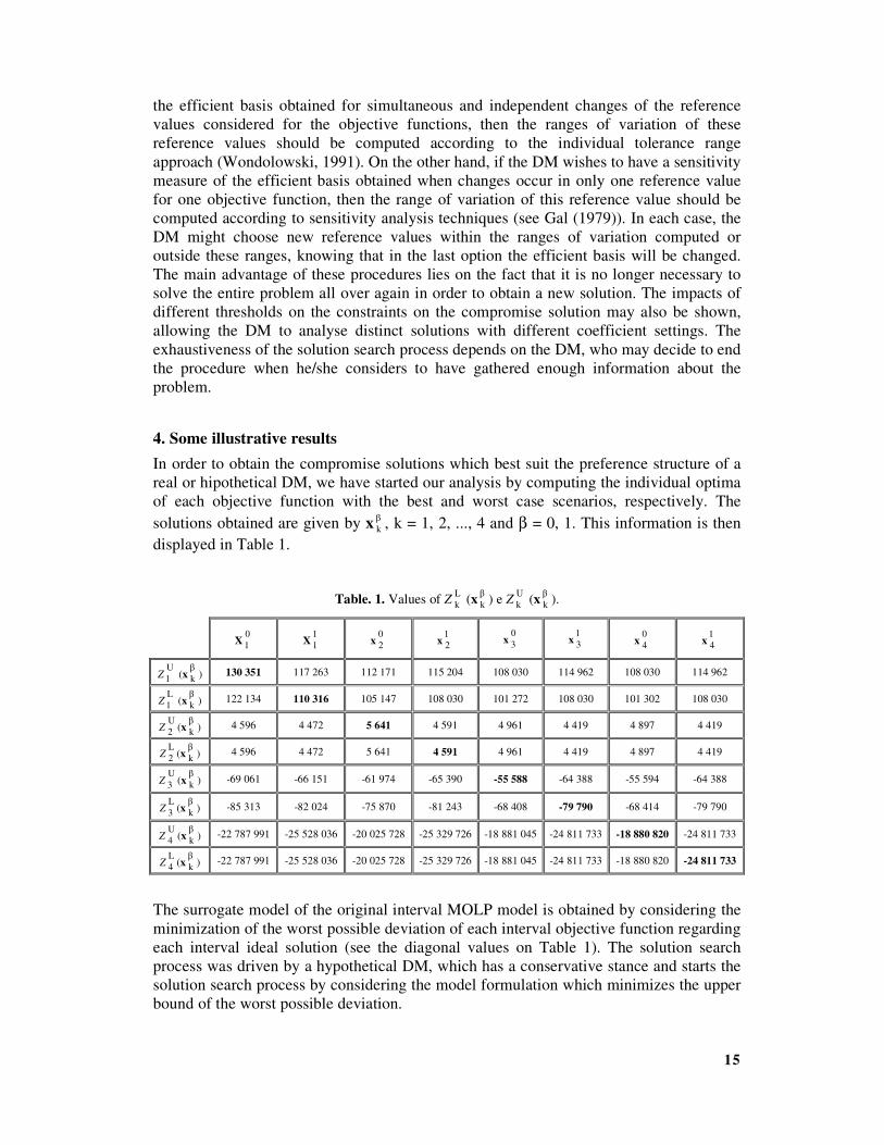
4. Some illustrative results
In order to obtain the compromise solutions which best suit the preference structure of a
real or hipothetical DM, we have started our analysis by computing the individual optima
of each objective function with the best and worst case scenarios, respectively. The
solutions obtained are given by x β
k , k = 1, 2, ..., 4 and β = 0, 1. This information is then
displayed in Table 1.
Table. 1. Values of ZL
k (xβ
k ) e ZU
k (xβ
k ).
X0
1 X1
1 x0
2 x1
2 x0
3 x
1
3 x
0
4 x1
4
ZU
1 (xβ
k ) 130 351 117 263 112 171 115 204 108 030 114 962 108 030 114 962
ZL
1 (xβ
k ) 122 134 110 316 105 147 108 030 101 272 108 030 101 302 108 030
ZU
2 (xβ
k ) 4 596 4 472 5 641 4 591 4 961 4 419 4 897 4 419
ZL
2 (xβ
k ) 4 596 4 472 5 641 4 591 4 961 4 419 4 897 4 419
ZU
3 (xβ
k ) -69 061 -66 151 -61 974 -65 390 -55 588 -64 388 -55 594 -64 388
ZL
3(xβ
k ) -85 313 -82 024 -75 870 -81 243 -68 408 -79 790 -68 414 -79 790
ZU
4 (xβ
k ) -22 787 991 -25 528 036 -20 025 728 -25 329 726 -18 881 045 -24 811 733 -18 880 820 -24 811 733
ZL
4 (xβ
k ) -22 787 991 -25 528 036 -20 025 728 -25 329 726 -18 881 045 -24 811 733 -18 880 820 -24 811 733
The surrogate model of the original interval MOLP model is obtained by considering the
minimization of the worst possible deviation of each interval objective function regarding
each interval ideal solution (see the diagonal values on Table 1). The solution search
process was driven by a hypothetical DM, which has a conservative stance and starts the
solution search process by considering the model formulation which minimizes the upper
bound of the worst possible deviation.

16
In order to obtain a global overview of the model with this formulation we have started
our analysis by considering four coefficient settings with satisfaction thresholds on the
constraints of 1, 0.8, 0.5 and 0, respectively.
The solutions obtained are briefly characterized as follows.
Solution x1U’’
, obtained with the most constrained version of the feasible region, allows
achieving the worst optimum of GWP and energy imports (solutions x 1
3 and x1
4 ).
Solution x2U’’
, obtained with a relatively constrained coefficients setting, allows
improving the upper bounds on the environment and energy objectives (regarding the
previous solution). However, the lower bounds of these objective functions are now
farther from the lower bounds of the corresponding interval ideal solutions (the
achievement rates of the lower bounds of these objective functions are now higher than
one). Nevertheless, from the acceptability index and the distance between intervals, it
might be concluded that the interval objective functions regarding energetic and
environmental concerns (GWP) and the corresponding interval ideal solutions are now
closer. On the other hand, the economic (GDP) and social (employment) axes of
evaluation have lower values, having in the last situation both achievement rates with
negative values (Table 2). This situation might occur, since the minimum of each
objective function in the trade-off table is a convenient minimum and it might not be the
real minimum of the objective function in the feasible region.
Table 2. Information regarding solution x2U’’
.
ZL
k(x2U’’) Z
U
k(x2U’’) m[Zk(x
2U’’)] w[Zk(x2U’’)] A (Zk(x
2U’’) p Zk*) d(Zk
*, Zk(x2U’’)) tc
L
k tc
U
k
Z1 106 668 113 478 110 073 6 810 0.76 16 872.82 0.60 0.24
Z2 4 363 4 363 4 363 0 1.43 1 278.36 -0.33 -0.05
Z3 -77 116 -62 362 -69 739 14 753 0.11 6 774.39 1.48 0.50
Z4 -23 399 299 -23 399 299 -23 399 299 0 0.52 4 518 479.40 2.97 0.32
Solution x3U’’
, obtained with an intermediate coefficients setting, allows improving the
upper bounds of the environmental and energetic objectives, regarding the two solutions
previously analysed. However, the lower bounds of these objective functions regarding
the lower bounds of their corresponding interval ideal solutions are now more distant.
Nevertheless, from the acceptability index (with values near zero) and the distance
between intervals, we may conclude that the interval objective functions and the
corresponding interval ideal solutions are closer. On the other hand, the economic and
social axes of evaluation are worsened (Table 3).
Table 3. Information regarding solution x3U’’
.
ZL
k(x3U’’) Z
U
k(x3U’’) m[Zk(x
3U’’)] w[Zk(x3U’’)] A (Zk(x
3U’’) p Zk*) d(Zk
*, Zk(x3U’’)) Tc
L
k tc
U
k
Z1 104 534 111 526 108 030 6 992 0.91 18 825.05 0.36 0.16
Z2 4 263 4 263 4 263 0 1.63 1 378.33 -0.91 -0.13
Z3 -74 710 -60 669 -67 689 14 041 0.00 5 080.98 1.92 0.62
Z4 -21 662 240 -21 662 240 -21 662 240 0 -0.06 3 149 962.63 5.40 0.58

17
Solution x4U’’
, obtained with a less constrained coefficients setting, allows improving the
upper and lower bounds of GDP, regarding the previous solutions, enabling it to be closer
to its interval ideal solution (the values of the acceptability index and of the distance
between intervals are now lower – see Table 4). On the other hand, the level of
employment reaches its worst optimum value (optimum value obtained with the worst
coefficients setting), leading to an improvement of both achievement rates. Nevertheless,
these solutions are not dominated from the point of view of the achievement rates of the
objective functions. In fact, in what concerns the results obtained in solution x4U’’
, in
solution x 1
2 , the achievement rates of GDP are deteriorated in both bounds; however, the
achievement rates of the lower bounds of GWP (0.74) and energy imports (0.28) are now
closer to one in absolute terms.
Table 4. Information regarding solution x4U’’.
ZL
k (x4U’’) Z
U
k (x4U’’) m[Zk(x4U’’)] w[Zk(x
4U’’)] A (Zk(x4U’’) p Zk
*) d(Zk*, Zk(x
4U’’)) tcL
k tc
U
k
Z1 109 544 116 213 112 879 6 669 0.56 14 137.66 0.91 0.37
Z2 4 591 4 591 4 591 0 1.00 1 049.56 1.00 0.14
Z3 -77 296 -62 098 -69 697 15 198 0.10 6 510.49 1.45 0.52
Z4 -21 935 126 -21 935 126 -21 935 126 0 0.03 3 054 306.36 5.02 0.54
Admitting that the DM does not consider any of the solutions obtained so far as
satisfactory, the quest for new solution continues. Suppose that the DM wants to evaluate
what would happen if he/she adopts a more optimistic stance. Hence, new solutions are
obtained by considering three coefficient settings with the following thresholds on the
constraints: 1, 0.5 and 0, corresponding to x1U’
, x2U’
and x3U’
, respectively. Regarding
these solutions: solution x1U’
is the one with the best environmental results and the worst
energy imports, economic and social results; solution x2U’
allows obtaining the worst
environmental outcomes (particularly in what concerns to AEP, TOP and to GWP with
the most favorable version of the coefficients setting) and the worst performance of the
public global balance, but the best economic and social effects; solution x3U’
is the one
which allows the best performance for the public global balance and the worst values for
GWP in its less favorable version and the lower level of energy imports.
Suppose that the DM wishes to analyse the solutions obtained by combining situations
more/less favorable in the scope of the energy coefficients settings (reduction/increase of
the energy consumption coefficients) with the environmental and economic coefficients
at their central values. Solution x4U’
and solution x5U’
are obtained with the most and less
favorable version of energy consumption coefficients, respectively. The results obtained
in these solutions indicate that the reduction of the energy consumption coefficients
(therefore, the improvement of energy consumption efficiency) leads to a positive
impulse on the economic growth (with the corresponding environmental impacts) and on
the employment in a more energy efficient way, that is with a lower requirement for
energy imports.
Let us now suppose that the DM wants to review its solution search process, by adopting
once more a conservative stance, but imposing minimum values to the lower bounds of
GDP, GWP and energy imports with the coefficients setting of solution x3U’’
(threshold
on the constraints of 0.5). Hence, the following constraints are added to the model:
Z L
1 (x) ≥ 120 000, Z L
3 (x) ≥ -76 022, Z L
4 (x) ≥ -18 881.

18
55000
60000
65000
70000
75000
80000
85000
90000
GWP
Lower bound
Upper bound
Coefficients setting
Target 2010
14000
16000
18000
20000
22000
24000
26000
28000
30000
AEP
Lower bound
Upper bound
Coefficients setting
Target 2010
Gotemburg Protocol
With this coefficients setting, the additional constraints lead to an empty feasible region.
Hence, an elastic LP problem is solved and a new solution (x5U’’
) is obtained. Thus,
regarding solution x3U’’
there is a slight improvement of the lower bound of GDP, of the
level of employment (which has the same value of its worst optimum), of the upper
bound of GWP and of the upper bound of energy imports. Although this solution allows
obtaining the individual optimum of the level of employment with the less favorable
version of the coefficients of the model, this solution is not dominated from the point of
view of the achievement rates of the objective functions (the same might be said about
x4U’’
) since it corresponds to higher outcomes on the environmental and energetic plans.
On the other hand, the best results of GWP and energy imports are obtained when
compared to the other solutions analysed so far (see Figure 1).
Figure 1. Ranges of variation GWP and AEP in the solutions analysed.
The solution search process stops when the DM considers to have gathered enough
information on the problem.
5. Final remarks
Traditionally the I-O modeling approach has omitted any sources of uncertainty. The
inter/intra industrial linkages have generally been viewed as static and deterministic. This
paper proposes a MOLP model based on I-O analysis, which allows the analysts/DMs to
assess impacts on the economy at a macroeconomic level, the environment and the
energy system, based on the levels of activity of industrial sectors, in a situation of
uncertain data modeled through interval coefficients. The aim is to provide information
regarding robust solutions, that is, efficient solutions which attain desired levels for the
objective functions across a set of plausible scenarios. The solution search process has
been driven by considering a hypothetical DM which expresses his/her preferences
regarding the information presented. In this case, we have opted to perform the solution
search process by considering distinct decision alternatives according to a more or less
conservative stance of the DM. By analyzing globally the solutions obtained with both
formulations we can conclude that, in general, the more conservative stance allows
obtaining better results for the energetic and environmental objectives; on the other hand,
with the less conservative stance better outcomes are obtained for the economic and
social concerns. All the solutions obtained indicate the need to reduce the energy
intensity of the economy in order to overcome the deficit regarding the Kyoto Protocol
fulfillment. Then again, it might be said that the improvement of energy efficiency is not
enough to attain the necessary emissions reduction in order to achieve the targets imposed
19
on the acidifying substances, being necessary to operate substantial changes namely on
the electricity generation sector.
References
Antunes, C. H., C. Oliveira, J. Clímaco, A study of the interactions between the energy
system and the economy using TRIMAP. In. D. Bouyssou, E. Jacquet-Lagrèze, P. Perny,
R. Slowinski, D. Vanderpooten, P. Vincke (Eds.), Aiding Decisions with multiple criteria
- Essays in Honor of Bernard Roy, 407–427, Kluwer Academic Publishers, 2002.
Chinneck, J.W., E. W. Dravnieks, Locating minimal infeasible constraint sets in linear
programs, ORSA Journal on Computing, Vol 3, nº 2, 157–168, 1991.
Chinneck, J.W., K. Ramadan, Linear programming with interval coefficients, Journal of
the Operational Research Society, Vol. 51, nº 2, 209–220, 2000.
Dorfman, R., P. A. Samuelson and R. M. Solow, Linear programming and economic
analysis, New York: Dover Publications, Inc., 1958.
Ferreira, V. G, T. C. Pereira, T. Seabra, P. Torres, H. Maciel, Portuguese national
inventory report on greenhouse gases, 1990 – 2004, Submitted under the United Nations
Framework Convention on Climate Change, Instituto do Ambiente (Ed.), 2006.
Gal, Tomas, Postoptimal analysis, parametric programming and related topics,
McGraw-Hill Inc, 1979.
Hawdon, D., P. Pearson, Input-output simulations of energy, environment, economy
interactions in the UK, Energy Economics,Vol. 17, nº 1, 73-86, 1995.
Instituto do Ambiente, Departamento de Ciências e Engenharia do Ambiente, FCT/UNL,
Centro de Estudos em Economia da Energia, dos Transportes e do Ambiente, Programa
para os tectos de emissão nacional – Estudos de base – Cenário de referência, 2004b (in
portuguese).
Instituto do Ambiente, Relatório do estado do ambiente 2003, Amadora, 2005 (in
portuguese).
Inuiguchi, M., Y. Kume, Goal programming problems with interval coefficients and
target intervals, European Journal of Operational Research, Vol. 52, nº 3, 345–360, 1991.
IPCC, Revised 1996 IPCC guidelines for national greenhouse gas inventories: Reference
manual, 1996a.
IPCC, Revised 1996 IPCC guidelines for national greenhouse gas inventories: Reporting
instructions, 1996b.
IPCC, Revised 1996 IPCC guidelines for national greenhouse gas inventories: Workbook,
1996c.
IPCC, 2006 IPCC Guidelines for national greenhouse gas inventories: Energy, 2006.
Oliveira, C., C. H. Antunes, A multiple objective model to deal with economy-energy-
environment interactions, European Journal of Operational Research, Vol. 153, nº 2,
370–385, 2004.
Oliveira, C., C. H. Antunes, Multiple objective linear programming models with interval
coefficients – an illustrated overview, European Journal of Operational Research, Vol.
181, nº 3, 1434–1463, 2007.
Oliveira, C., C. H. Antunes, An interactive method to tackle uncertainty in interval
multiple objective linear programming, Journal of Mathematical Sciences, 2009 (in print).

20
Wondolowski, F. R., A generalization of Wendell’s tolerance approach to sensitivity
analysis in linear programming, Decision Sciences, Vol. 22, nº 4, 792–810, 1991.
Urli, B., R. Nadeau, An interactive method to multiobjective linear programming
problems with interval coefficients, INFOR, Vol. 30, nº 2, 127–137, 1992.
21
Appendix
Variable Description Unit Expression
x Vector of total output for each branch. 106 euros (at constant
basic prices) or toe.
(2.1), (2.10), (2.13), (2.14),
(2.15), (2.19), (2.21), (2.24),
(2.39), (2.45), (2.84)
impc
Vector of competitive imports. The elements which
correspond to non-energetic goods or services have null
value.
toe (2.1), (2.10), (2.84)
cptf Total consumption of the resident and non-resident
households on the territory.
106 euros (at constant
purchasers’ prices).
(2.1), (2.2), (2.10), (2.15),
(2.24), (2.33), (2.39), (2.45),
(2.54)
csf Total consumption of the NPISH. 106 euros (at constant
purchasers’ prices).
(2.1), (2.4), (2.10), (2.15),
(2.24), (2.33), (2.39), (2.45),
(2.54)
g Total public consumption 106 euros (at constant
purchasers’ prices).
(2.1), (2.10), (2.15), (2.17),
(2.24), (2.33), (2.39), (2.45)
fbcf Total gross fixed capital formation – GFCF. 106 euros (at constant
purchasers’ prices). (2.1), (2.10), (2.15), (2.17)
sc Total changes in inventories. 106 euros (at constant
purchasers’ prices).
(2.1), (2.10), (2.15), (2.17),
(2.18), (2.84)
acov Acquisitions less disposals of valuables – ALDV. 106 euros (at constant
purchasers’ prices).
(2.1), (2.10), (2.15), (2.17),
(2.18)
expstcif Total exports at purchasers’ CIF prices (excluding
tourism).
106 euros (at CIF
constant prices).
(2.1), (2.6), (2.7), (2.8),
(2.15)
cptfr Total consumption of the resident households on the
territory.
106 euros (at constant
purchasers’ prices). (2.2), (2.4)
cpe Total consumption of the non-resident households on the
territory (tourism exports).
106 euros (at constant
prices). (2.2), (2.9)
cpr Total consumption of resident households and NPISH. 106 euros (at constant
purchasers’ prices).
(2.3), (2.4), (2.5), (2.17),
(2.18)
yd Disposable income of the households and NPISH. 106 euros (at constant
prices). (2.3)
ydcorr Disposable income of the households and NPISH. 106 euros (at current
prices). (2.3), (2.20), (2.23)
pcpr Price deflator for the consumption of households and
NPISH (interval exogenous variable).
Allows converting
constant prices into
current prices
(2.3), (2.18), (2.21)
cpm Private consumption of the resident households out of
the territory (tourism imports).
106 euros (at constant
prices). (2.4), (2.5), (2.12)
expstfob Total exports at FOB purchasers’ prices (excluding
tourism).
106 euros (at constant
FOB prices). (2.6), (2.9)
impstcif Total imports at CIF basic prices (excluding tourism). 106 euros (at constant
CIF prices). (2.6), (2.10), (2.11)
expa Vector of exports of goods or services (excluding
tourism) at CIF purchasers’ prices.
106 euros (at constant
CIF prices). (2.7), (2.8)
expfob Total exports at FOB purchasers’ prices (including
tourism).
106 euros (at constant
FOB prices). (2.9), (2.17), (2.18)
mstfob Total imports at FOB prices (excluding tourism). 106 euros (at constant
FOB prices). (2.11), (2.12)
mfob Total imports at FOB prices (including tourism). 106 euros (at constant
FOB prices). (2.12), (2.17), (2.18)
vab Gross Added Value (GAV). 106 euros (at basic
constant prices). (2.13), (2.16)
emp Employment level. 103 full-time equivalent
persons. (2.14), (2.82)
ts Net taxes on goods and services. 106 euros (at constant
prices). (2.15), (2.16), (2.21)
pibprod GDP at constant market prices (production approach). 106 euros (at constant
prices). (2.16)
pib GDP at constant market prices (expenditure approach). 106 euros (at constant
prices). (2.17), (2.81)
pibcorr GDP at current market prices. 106 euros (at current
prices). (2.18), (2.20), (2.23)
gcorr Public consumption 106 euros (at current
prices). (2.18), (2.23)
fbcfcorr GFCF. 106 euros (at current
prices). (2.18)
psc Price deflator for changes in inventories (interval
exogenous variable). n.a. (2.18)
pacov Price deflator for ALDV (interval exogenous variable). n.a. (2.18)

22
Variable Description Unit Expression
pexpfob Price deflator for total exports at FOB prices (interval
exogenous variable). n.a. (2.18)
pmfob Price deflator for total imports at FOB prices (interval
exogenous variable). n.a. (2.18)
remcorr Wages and salaries. 106 euros (at current
prices). (2.19), (2.20), (2.23)
iucl Index of the unitary labor costs (interval exogenous
variable). n.a. (2.19)
rp+- rp- Balance of primary incomes with the rest of the world. 106 euros (at current
prices). (2.20)
tisub Total indirect taxes. 106 euros (at current
prices). (2.20), (2.21), (2.23)
tre Balance of private transfers with the rest of the world. 106 euros (at current
prices). (2.20)
trig Balance of internal transfers from the public
administrations to households.
106 euros (at current
prices). (2.20), (2.23)
itis Index of the average indirect tax rate (exogenous interval
variable). n.a. (2.21)
div Public debt. 106 euros (at current
prices). (2.22), (2.23)
div-1 Public debt of the previous period. 106 euros (at current
prices). (2.22), (2.23)
(sgg+ - sgg-) Public balance. 106 euros (at current
prices). (2.22), (2.23)
dat Public debt adjustment. 106 euros (at current
prices). (2.22)
rg Public debt interest rate (exogenous interval variable) % (2.23)
treg Balance of public transfers with the rest of the world. 106 euros (at current
prices). (2.23)
trkg Balance of the public capital transfers. 106 euros (at current
prices). (2.23)
gfbcf Public investment on GFCF. 106 euros (at current
prices). (2.23)
ecco2E Vector of total CO2 emissions from fuel combustion by
energy type. Gg. (2.24), (2.25)
ecco2 Total CO2 emissions from fuel combustion. Gg (2.25), (2.77)
ecelectw Total emissions of pollutant w (excluding CO2) from
energy combustion in electricity generation. Gg (2.26), (2.34)
xelect Sub-vector of x with the output of electricity for each
electricity generation type (excluding co-generation). toe (2.26)
eccogw Total emissions of pollutant w (excluding CO2) from
energy combustion in co-generation. Gg (2.27), (2.34)
xcog Element of x with the output of co-generation. toe (2.27)
ecrefw Total emissions of pollutant w (excluding CO2) from
energy combustion in refineries. Gg (2.28), (2.34)
xref Element of x with the output of refineries. toe (2.28), (2.35), (2.36), (2.40)
ecindw
Total emissions of pollutant w (excluding CO2) from
energy combustion in the industrial and construction
branches.
Gg (2.29), (2.34)
xind Sub-vector of x with the output of industrial and
construction branches.
106 euros (at constant
basic prices). (2.29)
ectrtw
Emissions of pollutant w (excluding CO2) from energy
combustion in the transportation branches t (t = 60 =
road and rail, 61 = maritime, 62 = air).
Gg (2.30), (2.34)
xt Element of x with the output of transportation branch t. 106 euros (at constant
basic prices). (2.30)
ecosyw Emissions of pollutant w (excluding CO2) from energy
combustion in branch y. Gg (2.32), (2.34)
xy Element of x with the output of branch y. 106 euros (at constant
basic prices).
(2.32), (2.48), (2.49), (2.50),
(2.51), (2.52), (2.54), (2.62),
(2.63)
eccpw Emissions of pollutant w (excluding CO2) from energy
combustion in final consumption. Gg (2.33), (2.34)
ecw Total emissions of pollutant w (excluding CO2) from
energy combustion. Gg.
(2.34), (2.70), (2.71), (2.72),
(2.73), (2.74), (2.75), (2.76)
eftpbw Fugitive emissions of pollutant w from the distribution,
storage and processing of crude oil. Gg (2.35), (2.42)
efppw Fugitive emissions of pollutant w from the processing of
oil products. Gg (2.36), (2.42)
efdistw Fugitive emissions of pollutant w from the sales of
gasoline. Gg (2.37), (2.42)
xgasolina Element of x with the output of gasoline. toe (2.37), (2.38)

23
Variable Description Unit Expression
efabastw Fugitive emissions of pollutant w from vehicle supply. Gg (2.38), (2.42)
efgnw Fugitive emissions of pollutant w from the
transmission/distribution of natural gas. Gg (2.39), (2.42)
efventw Fugitive emissions of pollutant w from venting and
flaring in the refining sector. Gg (2.40), (2.42)
efgeotw Fugitive emissions of pollutant w from geothermal
energy. Gg (2.41), (2.42)
xgeot Element of x with the output of geothermal energy. tep (2.41)
efw Total fugitive emission of pollutant w. Gg
(2.42), (2.70), (2.71), (2.72),
(2.73), (2.74), (2.75), (2.76),
(2.77)
eprjw Fugitive emissions of pollutant w from industrial
processes in branch j. Gg (2.43), (2.44)
xj Element of x with the output of branch j. 106 euros (at constant
basic prices).
(2.43), (2.46), (2.59), (2.61),
(2.63)
eprw Total emissions of pollutant w from industrial processes. Gg
(2.44), (2.70), (2.71), (2.72),
(2.73), (2.74), (2.75), (2.76),
(2.77)
efsolvw Fugitive emissions of pollutant w referring to the use of
solvents (non-energetic oil). Gg (2.45), (2.47)
efoutjw Fugitive emissions of pollutant w referring to the use of
other products in branch j. Gg (2.46), (2.47)
efsolvoutw Total fugitive emissions of pollutant w referring to the
use of solvents and other products. Gg
(2.47), (2.70), (2.71), (2.72),
(2.73), (2.74), (2.75), (2.76),
(2.77)
egterw Emissions of pollutant w (excluding CO2) regarding
animal type, r, in branch 1. Gg (2.48), (2.49), (2.53)
efentrw Emissions of CH4 from enteric fermentation, for each
animal type, r, in branch 1. Gg (2.50), (2.53)
eqraaw
Emissions of pollutant w (excluding CO2) from de
burning of agricultural residues according to crop
production, a.
Gg (2.51), (2.53)
efndw Emissions of pollutant w (excluding CO2) from the use
of nitrogen fertilizers according to their handling type, d. Gg (2.52), (2.53)
eagricw Total emissions of pollutant w (excluding CO2) from
agriculture activities. Gg
(2.53), (2.70), (2.71), (2.72),
(2.73), (2.74), (2.75), (2.76)
rsu Total generation of MSW in the territory. t (2.54), (2.55), (2.58), (2.63)
xcomserv
Sub-vector of x with the output of the service branches
(excluding sanitation, public hygiene and similar
services).
106 euros (at constant
basic prices). (2.54)
rsuaterrou Total amount of MSW of the type u going to SWDS. t (2.55)
ersuaterrouw Emission of pollutant w (excluding CO2) from waste of
type u going to SWDS. Gg (2.56), (2.57), (2.64)
rsuaterroun Total amount of MSW of the type u going to SWDS in
year n (exogenous variable from 1989 to 2009). t (2.56)
ersucompw Emission of pollutant w (excluding CO2) from anaerobic
digestion. Gg (2.58), (2.64)
eriborgaterrow Emission of pollutant w (excluding CO2) from industrial
waste going to SWDS. Gg (2.59), (2.60), (2.64)
eribincinw Emission of pollutant w from industrial waste
incineration. Gg (2.61), (2.64)
erhincinw Total emissions of pollutant w from hospital waste
incineration. Gg (2.62), (2.64)
eresincinw Total emissions of pollutant w from waste incineration. Gg (2.63), (2.64)
eresw Total emissions of pollutant w from waste management. Gg
(2.64), (2.70), (2.71), (2.72),
(2.73), (2.74), (2.75), (2.76),
(2.77)
tow Total degradable organic component in waste water. kg bod (biochemical
oxygen demand) /year (2.65), (2.66)
p Estimated population of the country for the planning year
(exogenous variable). 103 inhabitants (2.65), (2.67), (2.68)
eagddsw Total emissions of pollutant w (excluding CO2
emissions) from domestic waste water and sludge. Gg
(2.66), (2.67), (2.68), (2.70),
(2.71), (2.72), (2.73), (2.74),
(2.75), (2.76)
eagindw Total emissions of pollutant w (excluding CO2
emissions) from industrial waste water handling. Gg
(2.69), (2.70), (2.71), (2.72),
(2.73), (2.74), (2.75), (2.76)
dcind Degradable organic component of industrial waste water
(exogenous variable).
103 inhabitants
equivalent (2.69)
etco Total emissions of CO. Gg (2.70), (2.80)
etnox Total emissions of NOx. Gg (2.71), (2.79), (2.80)
etn2o Total emissions of N2O. Gg (2.72), (2.78)
etch4 Total emissions of CH4. Gg (2.73), (2.78), (2.80)

24
Variable Description Unit Expression
etcovnm Total emissions of NMVOC. Gg (2.74), (2.80)
etso2 Total emissions of SO2. Gg (2.75), (2.79)
etnh3 Total emissions of NH3. Gg (2.76), (2.79)
etco2 Total emissions of CO2. Gg (2.77), (2.78)
pag Global warming potential. Gg of CO2 equivalent (2.78), (2.83)
eac Acid equivalent potential. Gg of acid equivalent (2.79)
pfot Tropospheric ozone generating potential.. Gg of NMVOC
equivalent (2.80)
Coefficient Description Unit Expression
A
Technical coefficients matrix (product-
by-product). Each element, aij, is the
amount of good or service i needed to
produce a unit of good or service j. This
matrix has interval coefficients.
106 euros (at constant basic prices)/106 euros
(at constant basic prices) for flows between
non-energetic branches; 106 euros (at
constant basic prices)/toe for flows between
non-energetic and energetic branches;
toe/106 euros (at constant basic prices) for
flows between energetic and non-energetic
branches; toe/toe for flows between
energetic branches.
(2.1)
acptf
Vector with the weight of each good or
service aimed at household
consumption on the total household
consumption. This vector has interval
coefficients.
106 euros (at constant basic prices) or toe,
whether it is an energetic or non-energetic
branch, respectively/106 euros (at constant
purchasers’ prices).
(2.1)
acsf
Vector with the weight of each good or
service aimed at NPISH consumption
on the total NPISH consumption.
106 euros (at constant basic prices) or toe,
whether it is an energetic or non-energetic
branch, respectively/106 euros (at constant
purchasers’ prices).
(2.1)
ag
Vector with the weight of each good or
service aimed at public consumption on
the total public consumption.
106 euros (at constant basic prices) or toe,
whether it is an energetic or non-energetic
branch, respectively/106 euros (at constant
purchasers’ prices).
(2.1)
afbcf
Vector with the weight of each good or
service aimed at GFCF on the total
GFCF.
106 euros (at constant basic prices) or toe,
whether it is an energetic or non-energetic
branch, respectively/106 euros (at constant
purchasers’ prices).
(2.1)
asc
Vector with the weight of each good or
service aimed at changes in inventories
on the total changes in inventories.
106 euros (at constant basic prices) or toe,
whether it is an energetic or non-energetic
branch, respectively/106 euros (at constant
purchasers’ prices).
(2.1)
aacov
Vector with the weight of each good or
service aimed at ALDV on the total
ALDV.
106 euros (at constant basic prices) or toe,
whether it is an energetic or non-energetic
branch, respectively/106 euros (at constant
purchasers’ prices).
(2.1)
aexp
Vector with the weight of each good or
service aimed at exports at CIF prices
on the total exports (excluding tourism).
106 euros (at constant basic prices) or toe,
whether it is an energetic or non-energetic
branch, respectively/106 euros (at constant
purchasers’ prices).
(2.1), (2.7)
cptf* Upper interval bound on the household
consumption on the territory. 106 euros (at constant purchasers’ prices) (2.1)
csfL, csfU Upper and lower bounds on NPISH
consumption. 106 euros (at constant purchasers’ prices) (2.1)
gL, gU Upper and lower bounds on public
consumption. 106 euros (at constant purchasers’ prices) (2.1)
fbcfL, fbcfU Upper and lower bounds on GFCF. 106 euros (at constant purchasers’ prices) (2.1)
scL, scU Upper and lower bounds on changes in
inventories. 106 euros (at constant purchasers’ prices) (2.1)
acovL, acovU Upper and lower bounds on ALDV. 106 euros (at constant purchasers’ prices) (2.1)
expstcifL Lower bounds of exports (excluding
tourism) at CIF prices. 106 euros (at constant purchasers’ prices) (2.1)
cpe* Upper interval bound on the tourism
exports. 106 euros (at constant prices). (2.2)
β0 Autonomous household consumption. 106 euros (at constant purchasers’ prices). (2.3)
β1 Marginal propensity to consume
(interval coefficient).
106 euros (at constant purchasers’ prices)/
106 euros (at constant prices). (2.3)
cpr* Upper interval bound on the resident’s
household consumption. 106 euros (at constant purchasers’ prices). (2.3)
yd* Upper interval bound on the resident’s
disposable income. 106 euros (at constant prices). (2.3)
cptfr* Upper interval bound on the resident’s
household consumption on the territory. 106 euros (at constant purchasers’ prices). (2.4)

25
Coefficient Description Unit Expression
cpm* Upper interval bound on the tourism
imports. 106 euros (at constant prices). (2.4)
α Weight of the tourism imports on the
resident’s consumption. % (2.5)
aciffob CIF/FOB adjustment. 106 euros /106 euros (2.6), (2.11)
expstfob* Upper interval bound on exports
(excluding tourism) at FOB prices. 106 euros (at constant purchasers’ prices). (2.6)
impstcifL Lower bound on imports (excluding
tourism) at CIF prices. 106 euros (at constant purchasers’ prices). (2.6)
p̂ exp Diagonal matrix with convenient
dimensions which allows converting
export values from toe to euros.
Value one for non-energetic goods and
services; average unitary prices for each toe
in 106 euros (at constant basic prices) for
energetic goods or services.
(2.7)
aexpts
Vector with the weight of net taxes on
exports of goods and services on total
exports (excluding tourism).
106 euros (at constant prices)/ 106 euros (at
constant purchasers’ CIF prices). (2.7)
e1, e2, …, e21 Vector with ones with convenient
dimensions. n.a.
(2.8), (2.10), (2.15),
(2.25), (2.54), (2.84)
expfob* Upper interval bound of total exports at
FOB prices. 106 euros (at constant purchasers’ prices). (2.9)
pimpc
Vector which allows converting
competitive import values from toe to
euros.
Value one for non-energetic goods and
services; average unitary prices for each toe
in 106 euros (at constant CIF basic prices)
for energetic goods or services.
(2.10)
pimpnc
Vector which allows converting non-
competitive import values from toe to
euros.
Average unitary prices for each toe in 106
euros (at constant CIF basic prices) for
energetic goods or services
(2.10)
Amnc
Matrix of non-competitive import
coefficients of energy. toe/106 euros (at constant prices). (2.10), (2.84)
ascnc
Vector with the weight of changes in
inventories of non-competitive imports
of energy on the total changes in
inventories.
toe/106 euros (at constant purchasers’
prices). (2.10), (2.84)
Am
Matrix of non-competitive imports of
non-energetic goods or services
coefficients.
106 euros (at constant CIF basic prices)/ 106
euros (at constant basic prices). (2.10)
amcptf
Vector with the weights of non-
competitive imports of non-energetic
goods or services aimed at household
consumption on the total household
consumption on the territory.
106 euros (at constant CIF basic prices)/ 106
euros (at constant purchasers’ prices). (2.10)
amcsf
Vector with the weights of non-
competitive imports of non-energetic
goods or services aimed at NPISH
consumption on the total NPISH
consumption.
106 euros (at constant CIF basic prices)/ 106
euros (at constant purchasers’ prices). (2.10)
amg
Vector with the weights of non-
competitive imports of non-energetic
goods or services aimed at public
consumption on the total public
consumption.
106 euros (at constant CIF basic prices)/ 106
euros (at constant purchasers’ prices). (2.10)
amfbcf
Vector with the weights of non-
competitive imports of non-energetic
goods or services aimed at GFCF on the
total GFCF.
106 euros (at constant CIF basic prices)/ 106
euros (at constant purchasers’ prices). (2.10)
amsc
Vector with the weights of non-
competitive imports of non-energetic
goods or services aimed at changes in
inventories on the total changes in
inventories.
106 euros (at constant CIF basic prices)/ 106
euros (at constant purchasers’ prices). (2.10)
amacov
Vector with the weights of non-
competitive imports of non-energetic
goods or services aimed at ALDV on
the total ALDV.
106 euros (at constant CIF basic prices)/ 106
euros (at constant purchasers’ prices). (2.10)
mstfob* Upper interval bound of total imports
(excluding tourism) at FOB prices.
106 euros (at constant FOB purchasers’
prices) (2.11)
mstfob* Upper interval bound of total imports at
FOB prices.
106 euros (at constant FOB purchasers’
prices) (2.12)
arem Vector with the weights of wages on the
total output of each branch.
106 euros (at constant prices)/ 106 euros (at
constant basic prices). (2.13), (2.19)
aot Vector with the weights of taxes on the
total output of each branch.
106 euros (at constant prices)/ 106 euros (at
constant basic prices). (2.13), (2.21)

26
Coefficient Description Unit Expression
aos Vector with the weights of subsidies on
the total output of each branch.
106 euros (at constant prices)/ 106 euros (at
constant basic prices). (2.13), (2.21)
aebermb
Vector with the weight of gross
operating surplus and gross mixed
incomes on the total output of each
branch.
106 euros (at constant prices)/ 106 euros (at
constant basic prices). (2.13)
l
Vector with the ratio between the
number of employees in each branch (at
full-time equivalent person) and the
total output of each branch.
103 persons (at full-time equivalent person)/
106 euros (at constant basic prices). (2.14)
Ats
Matrix with the weights of net taxes on
goods and services on the total output of
each branch.
106 euros (at constant prices)/ 106 euros (at
constant basic prices). (2.15)
acptfts
Vector with the weights of net taxes on
goods and services aimed at household
consumption on total household
consumption on the territory.
106 euros (at constant prices)/ 106 euros (at
constant purchasers’ prices). (2.15)
acsfts
Vector with the weights of net taxes on
goods and services aimed at NPISH
consumption on the total NPISH
consumption.
106 euros (at constant prices)/ 106 euros (at
constant purchasers’ prices). (2.15)
agts
Vector with the weights of net taxes on
goods and services aimed at public
consumption on the total public
consumption.
106 euros (at constant prices)/ 106 euros (at
constant purchasers’ prices). (2.15)
afbcfts
Vector with the weights of net taxes on
goods and services aimed at GFCF on
total GFCF.
106 euros (at constant prices)/ 106 euros (at
constant purchasers’ prices). (2.15)
ascts
Vector with the weights of net taxes on
goods and services aimed at changes in
inventories on total changes in
inventories.
106 euros (at constant prices)/ 106 euros (at
constant purchasers’ prices). (2.15)
aacovts
Vector with the weights of net taxes on
goods and services aimed at ALDV on
total ALDV.
106 euros (at constant prices)/ 106 euros (at
constant purchasers’ prices). (2.15)
aexts
Vector with the weights of net taxes on
goods and services aimed at exports on
total exports.
106 euros (at constant prices)/ 106 euros (at
constant CIF purchasers’ prices). (2.15)
Atsnc
Matrix with the weights of net taxes on
non-competitive imports of energy on
the total output of each branch.
106 euros (at constant prices)/ 106 euros (at
constant basic prices). (2.15)
tsL Lower bound on total net taxes on
goods and services. 106 euros (at constant prices). (2.15)
pibL Lower bound on GDP. 106 euros (at constant market prices). (2.16), (2.17)
pib* Upper interval bound on GDP. 106 euros (at constant market prices). (2.16), (2.17)
pibcorr* Upper interval bound on GDP. 106 euros (at current market prices). (2.18)
gcorrL,
gcorrU
Lower and upper bounds on public
consumption. 106 euros (at current prices). (2.18)
fbcfcorrL,
fbcfcorrU Lower and upper bounds on GFCF. 106 euros (at current prices). (2.18)
remcorr* Upper interval bound on wages and
salaries. 106 euros (at current prices). (2.19)
pspibcorr Corporations savings as a percentage of
GDP (interval coefficient). % (2.20)
tigts
Weight of net indirect taxes received by
the public sector on the total amount of
net indirect taxes at current prices
(interval coefficient).
% (2.20), (2.23)
rtdydcorr
Weight of direct taxes on the disposable
income of households and NPISH
(interval coefficient).
% (2.20), (2.23)
tdscpibcorr
Weight of direct taxes on the income of
corporations on the GDP at current
prices (interval coefficient).
% (2.20), (2.23)
tcss
Weight of social security contributions
received by the public sector on total
wages and salaries (interval coefficient).
% (2.20), (2.23)
repgpibcorr
Weight of corporations and property
incomes of public sector on GDP at
current prices (interval coefficient).
% (2.20), (2.23)
ydcorr* Upper interval bound on disposable
income. 106 euros (at current prices). (2.20)

27
Coefficient Description Unit Expression
rp*
Upper interval bound on balance of
primary incomes with the rest of the
world.
106 euros (at current prices). (2.20)
tisub* Upper interval bound on net indirect
taxes. 106 euros (at current prices). (2.20)
tisubg*
Upper interval bound on net indirect
taxes received by the public
administration.
106 euros (at current prices). (2.20)
tre* Upper interval bound on private
transfers with the rest of the world. 106 euros (at current prices). (2.20)
td*
Upper interval bound on direct taxes on
disposable income of households and
NPISH.
106 euros (at current prices). (2.20)
tdsc* Upper interval bound on direct taxes on
income of corporations. 106 euros (at current prices). (2.20)
css* Upper interval bound on social security
contributions. 106 euros (at current prices). (2.20)
repg*
Upper interval bound on corporations
and property incomes of the public
sector.
106 euros (at current prices). (2.20)
trig*
Upper interval bound on the balance of
internal transfers from the public
administrations to households.
106 euros (at current prices). (2.20)
div* Upper interval bound on public debt. 106 euros (at current prices). (2.22)
div-1* Lower interval bound on the public debt
of the previous period. 106 euros (at current prices). (2.22)
sgg* Lower interval bound of the public
balance. 106 euros (at current prices). (2.22)
dat* Lower interval bound on the adjustment
of the public debt. 106 euros (at current prices). (2.22)
tkpibcorr
Weight of capital taxes received by the
public sector on GDP at current prices
(interval coefficients).
% (2.23)
treg*
Upper interval bound on the balance of
public transfers with the rest of the
world.
106 euros (at current prices). (2.23)
jurg* Upper interval bound on the interests of
public debt. 106 euros (at current prices). (2.23)
tk* Upper interval bound on capital taxes. 106 euros (at current prices). (2.23)
trkg* Upper interval bound on public capital
transfers. 106 euros (at current prices). (2.23)
gfbcf* Upper interval bound on the public
investment on GFCF. 106 euros (at current prices). (2.23)
Eˆtjcf
Diagonal matrix with conversion factors
from toe to terajoules - TJ - for each
type of energy.
TJ/toe
(2.24), (2.26), (2.27),
(2.28), (2.29), (2.30),
(2.32), (2.33)
Eˆcef
Diagonal matrix, whose main elements
are the carbon (C) emission factors for
each type of energy (interval
coefficient).
Tonnes (t) of C by TJ (tC/TJ). (2.24)
Eˆocf
Diagonal matrix, whose main elements
are the fractions of carbon oxidized for
each type of energy.
% (2.24)
AE
Matrix with the coefficients of energy
use by each branch. It is composed by
the coefficients of energy use of A and
Amnc, as well as by the coefficients of
biomass use. It has interval coefficients.
toe/ 106 euros (at constant basic prices). (2.24)
acptfE
Vector with the coefficients of energy
use by the households. This vector is
composed by the coefficients of energy
use of acptf, as well as by the coefficients
of biomass use. The elements refering
to the non-competitive energy imports
are null. It has interval coefficients.
toe/ 106 euros (at constant purchasers’
prices). (2.24), (2.33)
acsfE
Vector with the coefficients of energy
use by the NPISH. This vector is
composed by the energy use
coefficients of acsf. The elements
refering to the non-competitive energy
imports and to the use of biomass are
null.
toe/ 106 euros (at constant purchasers’
prices). (2.24), (2.33)

28
Coefficient Description Unit Expression
agE
Vector with the coefficients of energy
use by the public sector. This vector is
composed by the energy use
coefficients of ag. The elements refering
to the non-competitive energy imports
and to the use of biomass are null.
toe/ 106 euros (at constant purchasers’
prices). (2.24), (2.33)
NE
Matrix with the coefficients of energy
use with non-energetic purpose for each
branch.
toe/ 106 euros (at constant basic prices) or
toe, whether it is an energetic or non-
energetic branch, respectively.
(2.24)
ancptfE
Vector with the coefficients of energy
use by the households with non-
energetic purpose.
toe/ 106 euros (at constant purchasers’
prices). (2.24)
ancsfE
Vector with the coefficients of energy
use by the NPISH with non-energetic
purpose.
toe/ 106 euros (at constant purchasers’
prices). (2.24)
angE
Vector with the coefficients of energy
use by the public sector with non-
energetic purpose.
toe/ 106 euros (at constant purchasers’
prices). (2.24)
12
44
Ratio between the molecular weights of
CO2 and C. n.a. (2.24), (2.63)
10-3 Factor which allows converting values
into Gg. Gg/t
(2.24); (2.48), (2.49),
(2.50), (2.56), (2.63)
fecelectw
Vector with the emission factors for
pollutant w (excluding CO2) from
energy combustion in electricity power
generation, for each type of energy (it
has interval coefficients). Non-energetic
oil has null emission factors.
g/TJ (2.26)
AEelect
Submatrix of AE with the coefficients of
energy consumption for each type of
electricity generation. This submatrix
has interval coefficients.
toe/toe (2.26)
10-9 Factor which allows converting values
into Gg. Gg/g
(2.26), (2.27), (2.28),
(2.29), (2.30), (2.32),
(2.33), (2.35), (2.36),
(2.37), (2.38), (2.39),
(2.40), (2.41), (2.43),
(2.45), (2.46), (2.51),
(2.52)
feccogw
Vector with the emission factors for
pollutant w (excluding CO2) from
energy combustion in co-generation, for
each type of energy (it has interval
coefficients). Non-energetic oil has null
emission factors.
g/TJ (2.27)
AE.cog
Column of AE with the coefficients of
energy consumption in co-generation (it
has interval coefficients).
toe/toe (2.27)
fecrefw
Vector with the emission factors for
pollutant w (excluding CO2) from
energy combustion in refineries, for
each type of energy (it has interval
coefficients).
g/TJ (2.28)
AE.ref
Column of AE with the coefficients of
energy consumption in the refineries (it
has interval coefficients).
toe/toe (2.28)
NE.ref
Column of NE with the coefficients of
energy consumption with non-
energectic purpose in the refineries.
toe/toe (2.28)
fecindw
Vector with the emission factors for
pollutant w (excluding CO2) from
energy combustion in manufacturing
industry and construction for each type
of energy (it has interval coefficients).
g/TJ (2.29)
AEind
Submatrix of AE with coefficients of
energy consumption for each industrial
branch. It has interval coefficients.
toe/106 euros (at constant basic prices). (2.29)
NEind
Submatrix of NE with coefficients of
energy consumption with non-energetic
purpose for each industrial branch.
toe/106 euros (at constant basic prices). (2.29)

29
Coefficient Description Unit Expression
fectrwt
Vector with the emission factors for
pollutant w (excluding CO2) from
energy combustion in the transport
branches (t = 60 = road and rail, 61 =
maritime, 62 = air), for each type of
energy. Non-energetic oil has null
emission factors. This vector has
interval coefficients.
g/TJ (2.30)
AE.t
Column of AE with the coefficients of
energy consumption in the transport
branches (it has interval coefficients).
toe/106 euros (at constant basic prices). (2.30)
fectrwct
SO2 (w = 6) emission factor from
energy combustion of type c in the
transport branches. Non-energetic oil
has null emission factors. The value
obtained is an element of fectrwt (it has
interval coefficients).
g/TJ (2.31)
2 Ratio between the molecular weights of
SO2 and the sulphur content. n.a. (2.31)
s Sulphur content in the fuel. % (2.31)
q Net calorific value of the fuel. TJ/Gg (2.31)
109 Factor which allows converting Gg into
g. g/Gg (2.31)
r Sulphur retention in ash. % (2.31)
tred Abatement efficiency. % (2.31)
fecoswy
Vector with the emission factors for
pollutant w (excluding CO2) from
energy combustion in branch y, for each
type of energy. Non-energetic oil has
null emission factors. It has interval
coefficients.
g/TJ (2.32)
AE.y
Column of AE with the coefficients of
energy consumption in branch y (it has
interval coefficients).
toe/106 euros (at constant basic prices). (2.32)
feccpw
Vector with the emission factors for
pollutant w (excluding CO2) from
energy combustion in final
consumption, for each type of energy.
Non-energetic oil has null emission
factors. It has interval coefficients.
g/TJ (2.33)
apbref
Element of AE corresponding to the
coefficient of crude oil consumption in
the refining sector.
toe/toe (2.35)
fctpb Factor which allows converting values
from toe into t for crude oil. t/toe (2.35)
feftpbw
Fugitive emission factor of pollutant w
from crude oil transportation into
refineries.
g/t (2.35)
fefppw
Fugitive emission factor of pollutant w
from the processing of oil products
during refining activities.
g/toe (2.36)
fctgasolina Factor which allows converting values
from toe into t for gasoline. t/toe (2.37), (2.38)
fefdistw
Fugitive emission factor of pollutant w
regarding sales of gasoline from the
refinery to the service stations.
g/t (2.37)
fefabastw
Fugitive emission factor of pollutant w
from the sales of gasoline in the service
stations.
g/t (2.38)
AEgn.
Row vector of AE with the coefficients
of natural gas consumption for each
branch.
toe/106 euros (at constant basic prices). (2.39)
acptfgn
Element of acptfE with the coefficient of
natural gas consumption per unit of
household consumption on the territory.
toe/106 euros (at constant purchasers’
prices). (2.39)
acsfgn
Element of acsfE with the coefficient of
natural gas consumption per unit of
NPISH consumption.
toe/106 euros (at constant purchasers’
prices). (2.39)
aggn
Element of agE with the coefficient of
natural gas consumption per unit of
public consumption.
toe/106 euros (at constant purchasers’
prices). (2.39)
fctjgn Factor which allows converting values
from toe into TJ for natural gas. TJ/toe (2.39)
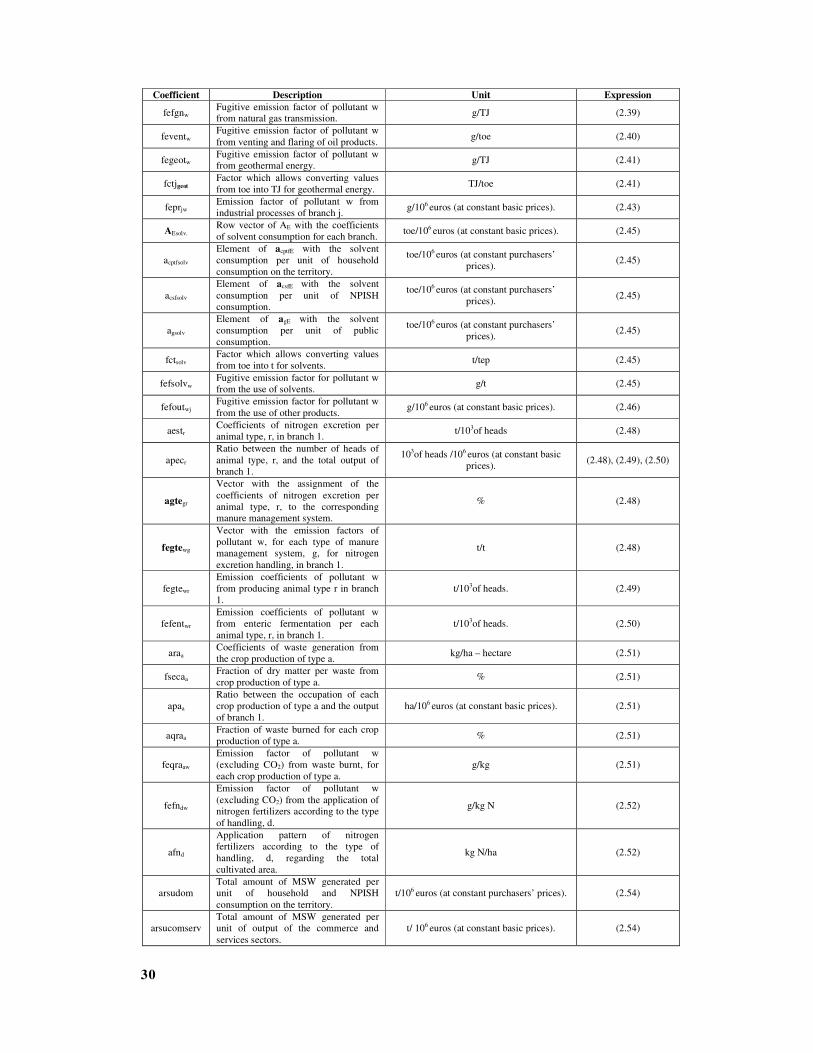
30
Coefficient Description Unit Expression
fefgnw Fugitive emission factor of pollutant w
from natural gas transmission. g/TJ (2.39)
feventw Fugitive emission factor of pollutant w
from venting and flaring of oil products. g/toe (2.40)
fegeotw Fugitive emission factor of pollutant w
from geothermal energy. g/TJ (2.41)
fctjgeot Factor which allows converting values
from toe into TJ for geothermal energy. TJ/toe (2.41)
feprjw Emission factor of pollutant w from
industrial processes of branch j. g/106 euros (at constant basic prices). (2.43)
AEsolv. Row vector of AE with the coefficients
of solvent consumption for each branch. toe/106 euros (at constant basic prices). (2.45)
acptfsolv
Element of acptfE with the solvent
consumption per unit of household
consumption on the territory.
toe/106 euros (at constant purchasers’
prices). (2.45)
acsfsolv
Element of acsfE with the solvent
consumption per unit of NPISH
consumption.
toe/106 euros (at constant purchasers’
prices). (2.45)
agsolv
Element of agE with the solvent
consumption per unit of public
consumption.
toe/106 euros (at constant purchasers’
prices). (2.45)
fctsolv Factor which allows converting values
from toe into t for solvents. t/tep (2.45)
fefsolvw Fugitive emission factor for pollutant w
from the use of solvents. g/t (2.45)
fefoutwj Fugitive emission factor for pollutant w
from the use of other products. g/106 euros (at constant basic prices). (2.46)
aestr Coefficients of nitrogen excretion per
animal type, r, in branch 1. t/103of heads (2.48)
apecr
Ratio between the number of heads of
animal type, r, and the total output of
branch 1.
103of heads /106 euros (at constant basic
prices). (2.48), (2.49), (2.50)
agtegr
Vector with the assignment of the
coefficients of nitrogen excretion per
animal type, r, to the corresponding
manure management system.
% (2.48)
fegtewg
Vector with the emission factors of
pollutant w, for each type of manure
management system, g, for nitrogen
excretion handling, in branch 1.
t/t (2.48)
fegtewr
Emission coefficients of pollutant w
from producing animal type r in branch
1.
t/103of heads. (2.49)
fefentwr
Emission coefficients of pollutant w
from enteric fermentation per each
animal type, r, in branch 1.
t/103of heads. (2.50)
araa Coefficients of waste generation from
the crop production of type a. kg/ha – hectare (2.51)
fsecaa Fraction of dry matter per waste from
crop production of type a. % (2.51)
apaa
Ratio between the occupation of each
crop production of type a and the output
of branch 1.
ha/106 euros (at constant basic prices). (2.51)
aqraa Fraction of waste burned for each crop
production of type a. % (2.51)
feqraaw
Emission factor of pollutant w
(excluding CO2) from waste burnt, for
each crop production of type a.
g/kg (2.51)
fefndw
Emission factor of pollutant w
(excluding CO2) from the application of
nitrogen fertilizers according to the type
of handling, d.
g/kg N (2.52)
afnd
Application pattern of nitrogen
fertilizers according to the type of
handling, d, regarding the total
cultivated area.
kg N/ha (2.52)
arsudom
Total amount of MSW generated per
unit of household and NPISH
consumption on the territory.
t/106 euros (at constant purchasers’ prices). (2.54)
arsucomserv
Total amount of MSW generated per
unit of output of the commerce and
services sectors.
t/ 106 euros (at constant basic prices). (2.54)

31
Coefficient Description Unit Expression
arsu90
Total amount of MSW handled and
treated per unit of output of sanitation,
public hygiene and similar services
branch.
t/ 106 euros (at constant basic prices). (2.54)
frsuaterro Fraction of waste going to SWDS. % (2.55)
aresiduou Fraction of waste of type u. % (2.55)
ku Methane generation rate for each type
of waste u. % (2.56)
mfcrsuu Methane correction factor for each type
of waste u. % (2.56)
docrsuu Degradable organic carbon for each
type of waste u. tC/t MSW (2.56)
docfrsuu Fraction of degradable organic carbon
dissimilated for each type of waste u. % (2.56)
fw Fraction of pollutant w in biogas. % (2.56)
12
16
Ratio between the molecular weights of
CH4 and C. n.a. (2.56)
n Year of waste deposition in SWDS. year (2.56)
2
Multiplication factor which assumes
that approximately 50% of the landfill
gas is CO2 and 50% is CH4.
n.a. (2.57), (2.60)
densch4 Density of CH4, which allows
converting the values from kg into m3. kg/m3 (2.57), (2.60)
106 Factor which allows converting Gg into
kg. kg/Gg (2.57), (2.60)
cconm Concentration of non organic methane
compounds (NMOC) in biogas. ppmv (2.57), (2.60)
10-6
Factor for correcting the concentration
of NMOC into units of ppmv.
Factor which allows converting kg into
Gg.
106 of parts/parts
Gg/kg
(2.57), (2.58), (2.60),
(2.61), (2.62), (2.66),
(2.67), (2.68), (2.69)
86.18 Molecular weight of NMOC as hexane. gmol (2.57), (2.60)
pop Operating pressure of the system 1 atm (2.57), (2.60)
(8.205)
(10-5)
Factor which allows converting NMOC
emissions into kg/year. m3 atm/gmol K (2.57), (2.60)
1000 Factor which allows converting kg into
g. g/kg (2.57), (2.60)
273 Factor which allows converting Celsius
degrees (0C) into K degrees. n.a. (2.57), (2.60)
top Temperature of the gas. 0C (2.57), (2.60)
covnm Fraction of NMVOC. % (2.57), (2.60)
frsucomp Fraction of waste assigned to anaerobic
digestion. % (2.58)
fersucomw
Emission factor of pollutant w from
anaerobic digestion of organic waste
(interval coefficient).
kg/t (2.58)
redemrsuw Abatement efficiency for pollutant w. % (2.58)
feriborgw Emission factor of pollutant w from
industrial waste deposition in SWDS. kg/t (2.59)
arij Total amount of industrial waste per
unit of output of branch j. t/ 106 euros (at constant basic prices). (2.59), (2.63)
fripri Fraction of hazardous wastes on the
total amount of industrial wastes. % (2.59), (2.63)
fribaterro Fraction of industrial wastes deposited
in SWDS. % (2.59)
friborgaterro Fraction of organic industrial wastes
deposited in SWDS. % (2.59)
fribincinsve Fraction of industrial waste which is
incinerated (with no energetic purpose). % (2.61)
feribincinw Emission factor of pollutant w from
industrial waste incineration. kg/t (2.61)
arhininc85
Amount of hospital waste incinerated
per unit of output of branch 85 (health
and social care).
t/ 106 euros (at constant basic prices). (2.62), (2.63)
ferhincinw Emission factor of pollutant w from the
hospital waste incineration. kg/t (2.62)
frsuincin
(fribincin)
Fraction of MSW (industrial waste)
which is incinerated. % (2.63)
ccrsurib Carbon content of MSW and industrial
wastes. % (2.63)

32
Coefficient Description Unit Expression
fcfrsubrib Fraction of fossil carbon in MSW and
industrial wastes. % (2.63)
ccrh Carbon content of hospital wastes. % (2.63)
fcfrh Fraction of fossil carbon in hospital
wastes. % (2.63)
efqueima Efficiency of combustion. % (2.63)
bod Per capita biochemical oxygen demand kg/103 of persons year (2.65)
feagd1w Emission factor of pollutant w from
domestic waste water handling. kg/kg bod (2.66)
ds Fraction of waste water converted into
sludge. % (2.66)
recagdtw Abatement efficiency for pollutant w. % (2.66)
fesdw Emission factor of pollutant w from
sludge handling. kg/kg bod (2.66)
recdsw Abatement efficiency for pollutant w. % (2.66)
feagd2w Emission factor of pollutant w from
nitrogen in domestic waste water. kg/kg N (2.67)
cprot Per capita protein. kg/103 inhabitants (2.67)
fnpr Fraction of Nitrogen in the protein. % (2.67)
fsepticas Fraction of the population served with
swage system. % (2.67)
feagd3w
Emission factor of pollutant w from
waste water handling, regarding the
volume of waste water handled.
kg/m3 (2.68)
cagd Volume of water supply per capita. m3/103 inhabitants (2.68)
fsaneamento Sanitation rate. % (2.68)
feagindw Emission factor of pollutant w from
industrial waste water handling. kg/103 inhabitants (2.69)
etcoU Upper bound on CO emissions. Gg (2.70)
etnoxU Upper bound on NOx emissions. Gg (2.71)
etn2oU Upper bound on N2O emissions. Gg (2.72)
etch4U Upper bound on CH4 emissions. Gg (2.73)
etcovnmU Upper bound on NMVOC emissions. Gg (2.74)
etso2U Upper bound on SO2 emissions. Gg (2.75)
etnh3U Upper bound on NH3 emissions. Gg (2.76)
etco2U Upper bound on CO2 emissions. Gg (2.77)
310 Factor which allows converting N2O
emissions into CO2 equivalent. Gg CO2 /Gg N2O (2.78)
21 Factor which allows converting CH4
emissions into CO2 equivalent. Gg CO2/Gg CH4 (2.78)
pagU Upper bound on GWP. Gg of CO2 equivalent (2.78)
21.74 Factor which allows converting NOx
emissions into acid equivalent. Acid equivalent/kg NOx (2.79)
31.25 Factor which allows converting SO2
emissions into acid equivalent. Acid equivalent /kg SO2 (2.79)
58.82 Factor which allows converting NH3
emissions into acid equivalent. Acid equivalent /kg NH3 (2.79)
eacU Upper bound on AEP Gg of acid equivalent. (2.79)
1.22 Factor which allows converting NOx
emissions into NMVOC equivalent. Gg NMVOC/Gg NOx (2.80)
0.11 Factor which allows converting CO
emissions into NMVOC equivalent. Gg NMVOC /Gg CO (2.80)
0.014 Factor which allows converting CH4
emissions into NMVOC equivalent. Gg NMVOC /Gg CH4 (2.80)
pfotU Upper bound on TOP. Gg of NMVOC equivalent. (2.80)