Institutionen för systemteknikDepartment of Electrical Engineering

Examensarbete

On Vergence Calibration of a Stereo Camera

Examensarbete utfört i Reglerteknikvid Tekniska högskolan vid Linköpings universitet

av

Sebastian Jansson

LiTH-ISY-EX--12/4627--SE

Linköping 2012

Department of Electrical Engineering Linköpings tekniska högskolaLinköpings universitet Linköpings universitetSE-581 83 Linköping, Sweden 581 83 Linköping

On Vergence Calibration of a Stereo Camera

Examensarbete utfört i Reglerteknikvid Tekniska högskolan vid Linköpings universitet

av

Sebastian Jansson

LiTH-ISY-EX--12/4627--SE

Handledare: Jonas Linderisy, Linköpings Universitet

Jon BjärkefurAutoliv Electronics

Emil NilssonAutoliv Electronics

Examinator: Thomas Schönisy, Linköpings Universitet

Linköping, 14 september 2012

Avdelning, InstitutionDivision, Department

Division of Automatic ControlDepartment of Electrical EngineeringSE-581 83 Linköping

DatumDate

2012-09-14

SpråkLanguage

� Svenska/Swedish

� Engelska/English

�

�

RapporttypReport category

� Licentiatavhandling

� Examensarbete

� C-uppsats

� D-uppsats

� Övrig rapport

�

�

URL för elektronisk version

http://www.ep.liu.se/

ISBN

—

ISRN

LiTH-ISY-EX--12/4627--SE

Serietitel och serienummerTitle of series, numbering

ISSN

—

TitelTitle On Vergence Calibration of a Stereo Camera

FörfattareAuthor

Sebastian Jansson

SammanfattningAbstract

Modern cars can be bought with camera systems that watch the road ahead. They can beused for many purposes, one use is to alert the driver when other cars are in the path ofcollision. If the warning system is to be reliable, the input data must be correct. One inputcan be the depth image from a stereo camera system; one reason for the depth image tobe wrong is if the vergence angle between the cameras are erroneously calibrated. Even ifthe calibration is accurate from production there’s a risk that the vergence changes due totemperature variations when the car is started.

This thesis proposes one solution for short-time live calibration of a stereo camera system;where the speedometer data available on the CAN-bus is used as reference. The motionof the car is estimated using visual odometry, which will be affected by any errors in thecalibration. The vergence angle is then altered virtually until the estimated speed is equal tothe reference speed.

The method is analyzed for noise and tested on real data. It is shown that detection ofcalibration errors down to 0.01 degrees is possible under certain circumstances using theproposed method.

NyckelordKeywords Ego-motion, Self-calibration, Stereo Calibration, Stereo Camera, Vergence Calibration, Vi-

sual Odometry

Abstract

Modern cars can be bought with camera systems that watch the road ahead. Theycan be used for many purposes, one use is to alert the driver when other cars arein the path of collision. If the warning system is to be reliable, the input datamust be correct. One input can be the depth image from a stereo camera system;one reason for the depth image to be wrong is if the vergence angle betweenthe cameras are erroneously calibrated. Even if the calibration is accurate fromproduction there’s a risk that the vergence changes due to temperature variationswhen the car is started.

This thesis proposes one solution for short-time live calibration of a stereo cam-era system; where the speedometer data available on the CAN-bus is used asreference. The motion of the car is estimated using visual odometry, which willbe affected by any errors in the calibration. The vergence angle is then alteredvirtually until the estimated speed is equal to the reference speed.

The method is analyzed for noise and tested on real data. It is shown that detec-tion of calibration errors down to 0.01 degrees is possible under certain circum-stances using the proposed method.

iii

Acknowledgments

Besides the people directly involved with my thesis, mentioned on the title page,I also would like to offer my special thanks to Fredrik Tjärnström at Autoliv forproviding me with the opportunity and general idea for the thesis.

In the same spirit I would like to show my appreciation for the help and generalexpertise provided by other employees of Autoliv.

I also want to acknowledge the help received from by Zoran Sjanic at ISY, LinköpingUniversity.

Finally I wish to thank Malin Persson and László Gönczi for help with proof-reading and making this report more accessible.

Linköping, September 2012Sebastian Jansson

v

Contents

1 Introduction 11.1 Background . . . . . . . . . . . . . . . . . . . . . . . . . . . 1

1.1.1 Visual Odometry . . . . . . . . . . . . . . . . . . . . 21.1.2 Vergence Calibration . . . . . . . . . . . . . . . . . . 2

1.2 Goals . . . . . . . . . . . . . . . . . . . . . . . . . . . . . . . 31.3 Exclusions . . . . . . . . . . . . . . . . . . . . . . . . . . . . 31.4 Method . . . . . . . . . . . . . . . . . . . . . . . . . . . . . . 4

2 Platform & notation 52.1 Stereo Vision System . . . . . . . . . . . . . . . . . . . . . . 52.2 Notation . . . . . . . . . . . . . . . . . . . . . . . . . . . . . 72.3 Coordinates . . . . . . . . . . . . . . . . . . . . . . . . . . . 8

3 Ego-motion 93.1 Camera motion and projection displacement . . . . . . . . . 10

3.1.1 From ego-motion to 2D-motion . . . . . . . . . . . . 103.1.2 Jacobian . . . . . . . . . . . . . . . . . . . . . . . . . 12

3.2 Displacement field method . . . . . . . . . . . . . . . . . . . 133.3 Direct method based on Lucas-Kanade tracker . . . . . . . . 143.4 Chosen method: Displacement field . . . . . . . . . . . . . . 173.5 Speed estimation noise sensitivity . . . . . . . . . . . . . . . 18

3.5.1 Displacement tracking error . . . . . . . . . . . . . . 183.5.2 Depth/disparity estimation error . . . . . . . . . . . 203.5.3 Yaw deviations . . . . . . . . . . . . . . . . . . . . . . 21

4 Vergence Calibration 234.1 Problem definition . . . . . . . . . . . . . . . . . . . . . . . 234.2 Estimating depth . . . . . . . . . . . . . . . . . . . . . . . . 244.3 Vergence estimation algorithm . . . . . . . . . . . . . . . . . 254.4 Speed estimation vergence sensitivity . . . . . . . . . . . . . 264.5 Vergence error calibration method . . . . . . . . . . . . . . . 27

5 Concluding remarks 335.1 Conclusion . . . . . . . . . . . . . . . . . . . . . . . . . . . . 335.2 Future work . . . . . . . . . . . . . . . . . . . . . . . . . . . 33

Bibliography 35

vii

viii CONTENTS

1Introduction

This thesis aim to develop a method to estimate the vergence angle for a stereocamera rig mounted within a car. It was done in cooperation with Autoliv Elec-tronics Sweden and with Linköping University.

1.1 Background

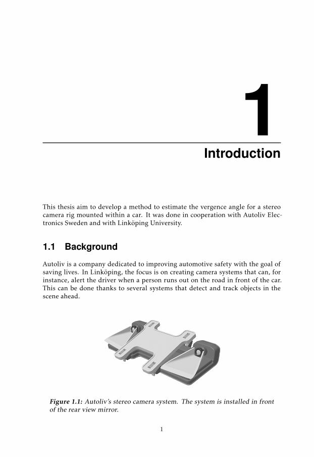
Autoliv is a company dedicated to improving automotive safety with the goal ofsaving lives. In Linköping, the focus is on creating camera systems that can, forinstance, alert the driver when a person runs out on the road in front of the car.This can be done thanks to several systems that detect and track objects in thescene ahead.

Figure 1.1: Autoliv’s stereo camera system. The system is installed in frontof the rear view mirror.

1

2 1 Introduction

Autoliv develops several products, one of which is a stereo camera system thatcan calculate depth, depicted in Figure 1.1. For a stereo vision system to workproperly, the system needs to be calibrated in some manner so that the pose1 ofthe cameras are known, otherwise the depth estimate will be inaccurate.

1.1.1 Visual Odometry

Visual odometry estimation, also called visual ego-motion estimation, is the pro-cess of estimating how the vehicle is moving based on image data from a camerasystem.

With high enough frame rates, it can be assumed that the motion will be smallin between frames. This is the basis for some ideas where the relation betweenmovement, relative to the camera, of a static point in a scene and the movementof its camera projection is linearized [Longuet-Higgins and Prazdny, 1980, Adiv,1985]. This concept is investigated in Irani et al. [1994] and further developedusing locally planar structures in Irani et al. [1997]. In Golban and Nedevschi[2011] it’s shown that the linearization does affect the result, but only to a limitedextent.

1.1.2 Vergence Calibration

In a stereo setup as the one used at Autoliv, the cameras are mounted firmlyto keep their relative pose fixed. The setup is then calibrated using calibrationtargets and camera calibration techniques. The calibration technique describedin Zhang [1999] is one of many which can do this.

Bγ

Left

Rightx

z

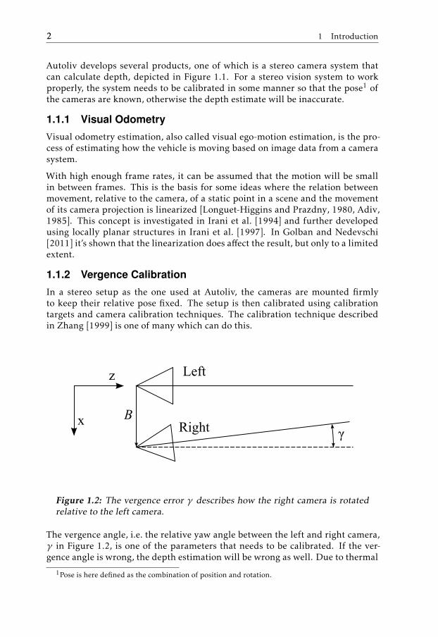
Figure 1.2: The vergence error γ describes how the right camera is rotatedrelative to the left camera.

The vergence angle, i.e. the relative yaw angle between the left and right camera,γ in Figure 1.2, is one of the parameters that needs to be calibrated. If the ver-gence angle is wrong, the depth estimation will be wrong as well. Due to thermal

1Pose is here defined as the combination of position and rotation.

1.2 Goals 3

variation, amongst other factors, the vergence angle can change over time. It’sdifficult to separate vergence error effects from actual differences in depth.

There are several techniques for self-calibration, i.e. calibration based on run-time input. Many such calibration techniques are described in Horaud et al.[2000]. Many of them are based on using a small number of frames and pointcorrespondences in some manner.

Horaud et al. [2000] continues to suggest a method for self-calibration usinghomographies2 describing the relationship between different camera views. InBrooks et al. [1996] a method for calibration is described using an analytical formof the fundamental matrix3 relating the left and right camera.

This thesis presents a different approach to the problem. The ego-motion esti-mation based on stereo data is compared with the information given by the car’sspeedometer. If the visual odometry is calculated for other reasons, this methodmight reduce the extra processing required. It also has potential to give goodresults in short time.

1.2 Goals

The goal of this master thesis is to design and evaluate a method for estimatingthe vergence angle between the two cameras in a stereo camera system mountedinside a car.

This has been divided into the following sub goals:

• Finding and implementing a method for visual odometry using stereo vi-sion data.

• Designing a method for calculating correct vergence using a comparison ofvisual odometry and mechanical odometry.

• Implement and evaluate the method within the development frameworkused at Autoliv.

1.3 Exclusions

The stereo images from Autoliv are rectified4 and the disparity is found usingcode that is available within Autoliv’s framework. This means that the thesiswork does not involve solving the problem of finding stereo disparity or the prob-lem of rectifying distorted images.

2A homography describes a mapping from the coordinates in one plane to coordinates in anotherplane using perspective transformation.

3The fundamental matrix for two 3D views describes how a point in one view relates to a line inthe other.

4Barrel distortion, lens distortion etc. are removed to create a pin-hole camera equivalent image.

4 1 Introduction

If the car owner has changed to tires with a different radius, the speedometerdata might be wrong. This has not been accounted for in this thesis, i.e. the speedfrom the speedometer is assumed to be true.

1.4 Method

At first, a theoretical study was performed on how to do visual odometry. Thisstudy was then the basis for the design of a method for finding visual odometryusing stereo data. This method was then implemented and tested on samplerecordings provided by Autoliv.

The effects of an error in vergence angle on the estimation were calculated. Thisresult was used to create a method of vergence angle extraction using mechanicaldata as a reference data source.

Finally, the method was implemented within the framework at Autoliv. The com-plete solution was then tested on recordings of the camera views for a vehicle inmotion where artificial calibration error was added.

2Platform & notation

This thesis was carried out at Autoliv, who have kindly provided developmentequipment and software as well as test data and systems. This chapter gives abrief description of the system used for development and testing. It also containsa short summary of the notation used in this thesis.

2.1 Stereo Vision System

Autoliv develops three different camera vision systems for cars.

• Night vision system with a FIR (Far Infrared Range, detects heat) camera

• Stereo vision system using normal cameras

• Mono vision system using normal cameras

In this thesis, the focus is on the stereo vision platform. The stereo vision systemconsists of two physically joined cameras 16 cm apart. The camera setup is placedin front of the rear view mirror.

The internal camera parameters, such as field of view, distance, angle and lensdistortion coefficients are estimated in a manually assisted calibration using cal-ibration targets. The images are rectified, that is, they are warped and rotatedaccording to the calibration so they are virtually looking straight forward.

Projections of objects at different distances have different translations when switch-ing between left and right camera. This parallax effect is used to estimate depth.

This is assisted by the calculation of a disparity map which encodes how eachpoint in the picture is translated between the left and right camera. This dis-

5

6 2 Platform & notation

Baseline

Left

Right

x

z

Depth

Disparity

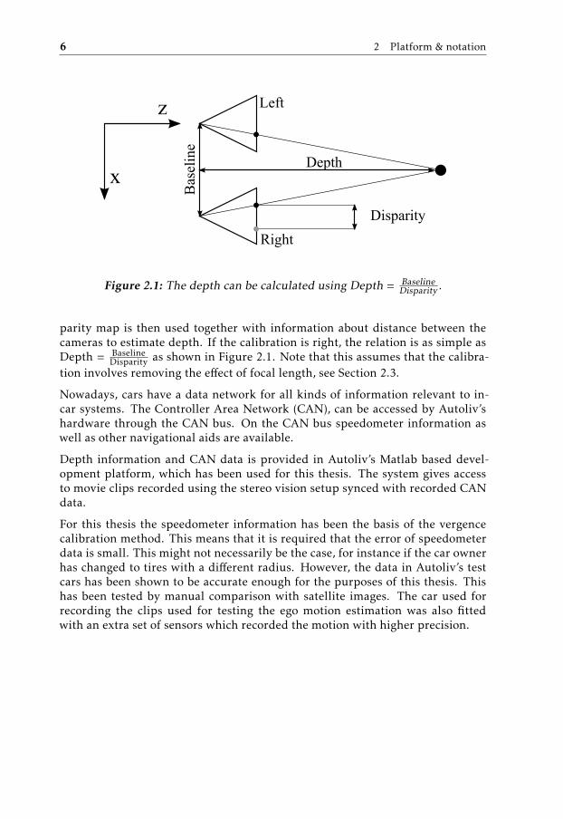
Figure 2.1: The depth can be calculated using Depth = BaselineDisparity .

parity map is then used together with information about distance between thecameras to estimate depth. If the calibration is right, the relation is as simple asDepth = Baseline

Disparity as shown in Figure 2.1. Note that this assumes that the calibra-tion involves removing the effect of focal length, see Section 2.3.

Nowadays, cars have a data network for all kinds of information relevant to in-car systems. The Controller Area Network (CAN), can be accessed by Autoliv’shardware through the CAN bus. On the CAN bus speedometer information aswell as other navigational aids are available.

Depth information and CAN data is provided in Autoliv’s Matlab based devel-opment platform, which has been used for this thesis. The system gives accessto movie clips recorded using the stereo vision setup synced with recorded CANdata.

For this thesis the speedometer information has been the basis of the vergencecalibration method. This means that it is required that the error of speedometerdata is small. This might not necessarily be the case, for instance if the car ownerhas changed to tires with a different radius. However, the data in Autoliv’s testcars has been shown to be accurate enough for the purposes of this thesis. Thishas been tested by manual comparison with satellite images. The car used forrecording the clips used for testing the ego motion estimation was also fittedwith an extra set of sensors which recorded the motion with higher precision.

2.2 Notation 7

2.2 Notation

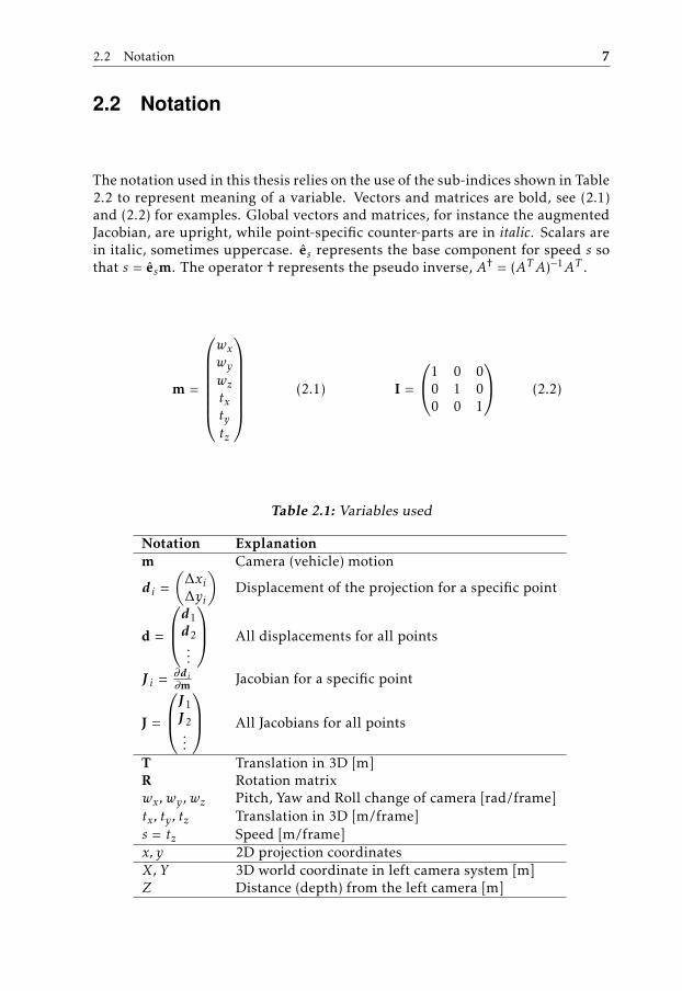
The notation used in this thesis relies on the use of the sub-indices shown in Table2.2 to represent meaning of a variable. Vectors and matrices are bold, see (2.1)and (2.2) for examples. Global vectors and matrices, for instance the augmentedJacobian, are upright, while point-specific counter-parts are in italic. Scalars arein italic, sometimes uppercase. es represents the base component for speed s sothat s = esm. The operator † represents the pseudo inverse, A† = (ATA)−1AT .

m =

wxwywztxtytz

(2.1) I =

1 0 00 1 00 0 1

(2.2)

Table 2.1: Variables used

Notation Explanationm Camera (vehicle) motion

di =(∆xi∆yi

)Displacement of the projection for a specific point

d =

d1d2...

All displacements for all points

J i = ∂di∂m Jacobian for a specific point

J =

J1J2...

All Jacobians for all points

T Translation in 3D [m]R Rotation matrixwx, wy , wz Pitch, Yaw and Roll change of camera [rad/frame]tx, ty , tz Translation in 3D [m/frame]s = tz Speed [m/frame]x, y 2D projection coordinatesX, Y 3D world coordinate in left camera system [m]Z Distance (depth) from the left camera [m]

8 2 Platform & notation

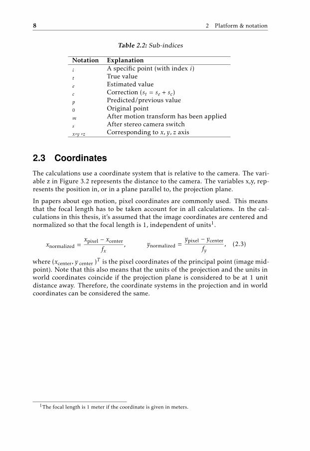
Table 2.2: Sub-indices

Notation Explanationi A specific point (with index i)t True valuee Estimated valuec Correction (st = se + sc)p Predicted/previous value0 Original pointm After motion transform has been applieds After stereo camera switchx,y ,z Corresponding to x, y, z axis

2.3 Coordinates

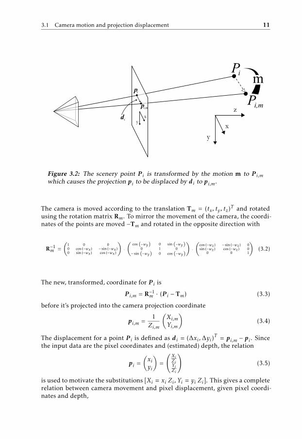
The calculations use a coordinate system that is relative to the camera. The vari-able z in Figure 3.2 represents the distance to the camera. The variables x,y, rep-resents the position in, or in a plane parallel to, the projection plane.

In papers about ego motion, pixel coordinates are commonly used. This meansthat the focal length has to be taken account for in all calculations. In the cal-culations in this thesis, it’s assumed that the image coordinates are centered andnormalized so that the focal length is 1, independent of units1.

xnormalized =xpixel − xcenter

fx, ynormalized =

ypixel − ycenter

fy, (2.3)

where (xcenter, y center )T is the pixel coordinates of the principal point (image mid-point). Note that this also means that the units of the projection and the units inworld coordinates coincide if the projection plane is considered to be at 1 unitdistance away. Therefore, the coordinate systems in the projection and in worldcoordinates can be considered the same.

1The focal length is 1 meter if the coordinate is given in meters.

3Ego-motion

Visual odometry estimation, also called visual ego-motion estimation, is the pro-cess of estimating how the camera, or the vehicle it’s mounted in, is moving basedon image data. The data available to do so in this case is two consecutive rectifiedpicture pairs from the stereo camera setup.

Since the method for estimating vergence investigated in this thesis is based onavailable ego-motion data, a method to acquire such data is required. In thischapter, a method for estimation of ego-motion based on previous work is de-scribed.

The stereo camera picture pair can be used to extract depth in the image. Ifthe baseline described in Chapter 2 is known, the depth will be correct in scale.If internal camera parameters are known as well, features in the image can bepositioned in 3D relative to the camera.

The idea used in this thesis is to combine information about the displacementof pixels in the 2D picture plane with information about their position in 3D.To do this, a mathematical relation between the two is derived. This relation isthen simplified to a linear model to make it usable for an in-car system wherecomputing power is limited.

Two methods of using this relation is then investigated. The first method tracksthe displacement for a set of picture coordinates within the image using sometracking algorithm. The inverse of the relation is then used to estimate the vehiclemotion that caused this displacement.

The second method works with the intensity images directly without going viatracked points. This is called a direct method, since it doesn’t use any intermedi-ate data.

9

10 3 Ego-motion

3.1 Camera motion and projection displacement

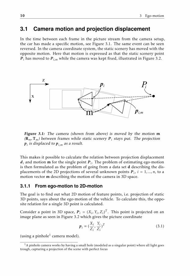
In the time between each frame in the picture stream from the camera setup,the car has made a specific motion, see Figure 3.1. The same event can be seenreversed. In the camera coordinate system, the static scenery has moved with theopposite motion. Here that motion is expressed as that the static scenery pointP i has moved to P i,m while the camera was kept fixed, illustrated in Figure 3.2.

pi Pi

pi,mm

x

z

Figure 3.1: The camera (shown from above) is moved by the motion m(Rm,Tm) between frames while static scenery P i stays put. The projectionpi is displaced to pi,m as a result.

This makes it possible to calculate the relation between projection displacementdi and motion m for the single point P i . The problem of estimating ego-motionis then formulated as the problem of going from a data set d describing the dis-placements of the 2D projections of several unknown points P i , i = 1, ..., n, to amotion vector m describing the motion of the camera in 3D space.

3.1.1 From ego-motion to 2D-motion

The goal is to find out what 2D motion of feature points, i.e. projection of static3D points, says about the ego-motion of the vehicle. To calculate this, the oppo-site relation for a single 3D point is calculated.

Consider a point in 3D space, P i = (Xi , Yi , Zi)T . This point is projected on animage plane as seen in Figure 3.2 which gives the picture coordinate

pi = (XiZi,YiZi

)T (3.1)

(using a pinhole1 camera model).

1A pinhole camera works by having a small hole (modeled as a singular point) where all light goestrough, capturing a projection of the scene with perfect focus

3.1 Camera motion and projection displacement 11

Pi

Pi,mz

xy

xy

pi

pi,m

di

m

Figure 3.2: The scenery point P i is transformed by the motion m to P i,mwhich causes the projection pi to be displaced by di to pi,m.

The camera is moved according to the translation Tm = (tx, ty , tz)T and rotatedusing the rotation matrix Rm. To mirror the movement of the camera, the coordi-nates of the points are moved −Tm and rotated in the opposite direction with

R−1m =

(1 0 00 cos (−wx ) − sin (−wx )0 sin (−wx ) cos (−wx )

)·

(cos

(−wy

)0 sin

(−wy

)0 1 0

− sin(−wy

)0 cos

(−wy

))

·

(cos (−wz ) − sin (−wz ) 0sin (−wz ) cos (−wz ) 0

0 0 1

)(3.2)

The new, transformed, coordinate for P i is

P i,m = R−1m · (P i − Tm) (3.3)

before it’s projected into the camera projection coordinate

pi,m =1Zi,m

(Xi,mYi,m

)(3.4)

The displacement for a point P i is defined as di = (∆xi ,∆yi)T = pi,m − pi . Since

the input data are the pixel coordinates and (estimated) depth, the relation

pi =(xiyi

)=

(XiZiYiZi

)(3.5)

is used to motivate the substitutions [Xi = xi Zi , Yi = yi Zi]. This gives a completerelation between camera movement and pixel displacement, given pixel coordi-nates and depth,

12 3 Ego-motion

di = f (m) = f (wx, wy , wz , tx, ty , tz) =(∆xi∆yi

)=

=

Cwy Swz (yi Zi−ty)+Cwy Cwz (xi Zi−tx)−Swy (Zi−tz )(Cwx Swy Swz−Swx Cwz) (yi Zi−ty)+(Swx Swz+Cwx Swy Cwz) (xi Zi−tx)+Cwx Cwy (Zi−tz )

− xi(Swx Swy Swz+Cwx Cwz) (yi Zi−ty)+(Swx Swy Cwz−Cwx Swz) (xi Zi−tx)+Swx Cwy (Zi−tz )(Cwx Swy Swz−Swx Cwz) (yi Zi−ty)+(Swx Swz+Cwx Swy Cwz) (xi Zi−tx)+Cwx Cwy (Zi−tz )

− yi

(3.6)

where S · = sin · and C · = cos · .

3.1.2 Jacobian

The Jacobian of (3.6) for a point Pi is

J i =∂ (∆xi ,∆yi)

∂(wx, wy , wz , tx, ty , tz

) ∣∣∣∣∣m=0

=

(xi yi −x2

i − 1 yi − 1Zi,m

0 xiZi,m

y2i + 1 −xi yi −xi 0 − 1

Zi,myiZi,m

)(3.7)

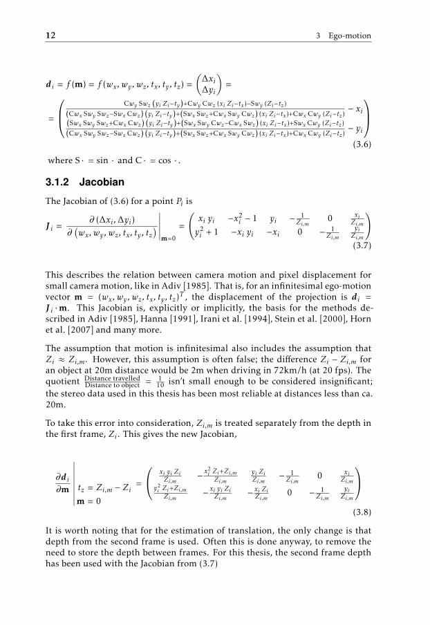
This describes the relation between camera motion and pixel displacement forsmall camera motion, like in Adiv [1985]. That is, for an infinitesimal ego-motionvector m = (wx, wy , wz , tx, ty , tz)T , the displacement of the projection is di =J i ·m. This Jacobian is, explicitly or implicitly, the basis for the methods de-scribed in Adiv [1985], Hanna [1991], Irani et al. [1994], Stein et al. [2000], Hornet al. [2007] and many more.

The assumption that motion is infinitesimal also includes the assumption thatZi ≈ Zi,m. However, this assumption is often false; the difference Zi − Zi,m foran object at 20m distance would be 2m when driving in 72km/h (at 20 fps). Thequotient Distance travelled

Distance to object = 110 isn’t small enough to be considered insignificant;

the stereo data used in this thesis has been most reliable at distances less than ca.20m.

To take this error into consideration, Zi,m is treated separately from the depth inthe first frame, Zi . This gives the new Jacobian,

∂di∂m

∣∣∣∣∣∣∣∣ tz = Zi,m − Zim = 0

=

xi yi ZiZi,m

− x2i Zi+Zi,mZi,m

yi ZiZi,m

− 1Zi,m

0 xiZi,m

y2i Zi+Zi,mZi,m

− xi yi ZiZi,m− xi ZiZi,m

0 − 1Zi,m

yiZi,m

(3.8)

It is worth noting that for the estimation of translation, the only change is thatdepth from the second frame is used. Often this is done anyway, to remove theneed to store the depth between frames. For this thesis, the second frame depthhas been used with the Jacobian from (3.7)

3.2 Displacement field method 13

3.2 Displacement field method

A common way to estimate ego motion is to find a number of easily tracked imagepoints and use the displacement of those image points between two frames to getthe motion of the camera. The augmented Jacobian matrix for all n points,

J =

J1J2...Jn

(3.9)

is here used as a model for how the projection of the same points are displacedbased on camera motion. The respective measured displacement for all points,

d =

d1d2...dn

(3.10)

is used as reference data. Since some data points might be wrong, a weighted leastsquare is used; the weights wi represents the probability that the tracked point ison a static object. The weighting is here based on a comparison of the motion ofa point to the expected motion based on previous motion. This is motivated bythe fact that the car can’t change motion very much between two frames. Giventhe previous motion mp, the Jacobian J i and the measured di , the weight of thespecific displacement is calculated as

wi = exp

(−∥∥di − J imp

∥∥2

2σ2

)(3.11)

where σ is the expected standard deviation in displacement error for inliers.

Finally the weighted least square solution is sought, where the squared differencebetween modeled displacement and reference displacement is minimized over allpossible vehicle motions,

minm

∑i

wi ‖J im − di‖2 (3.12)

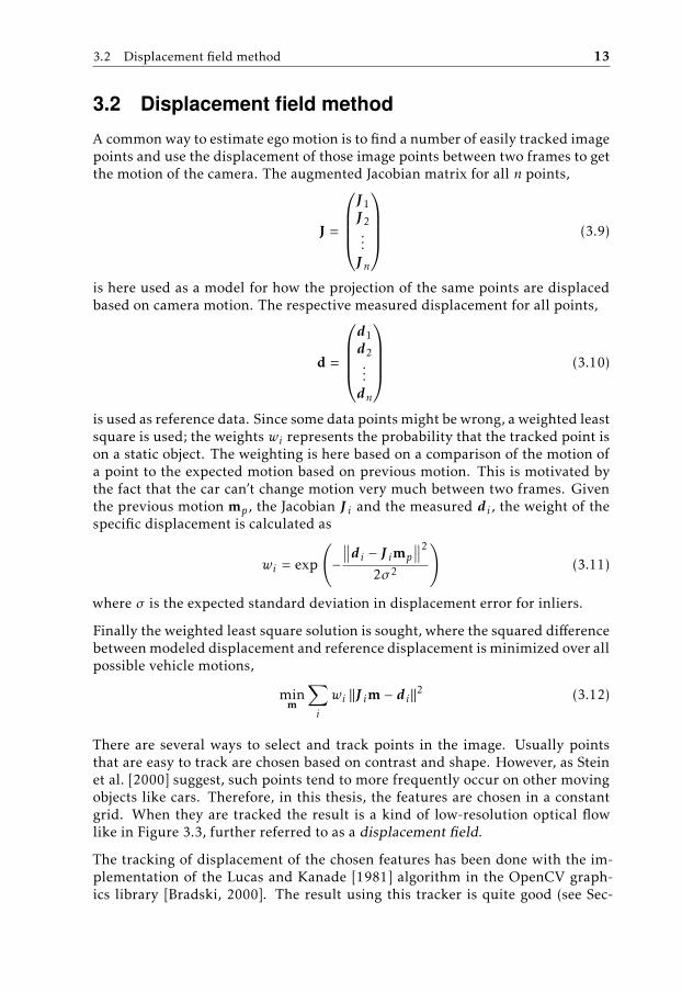
There are several ways to select and track points in the image. Usually pointsthat are easy to track are chosen based on contrast and shape. However, as Steinet al. [2000] suggest, such points tend to more frequently occur on other movingobjects like cars. Therefore, in this thesis, the features are chosen in a constantgrid. When they are tracked the result is a kind of low-resolution optical flowlike in Figure 3.3, further referred to as a displacement field.

The tracking of displacement of the chosen features has been done with the im-plementation of the Lucas and Kanade [1981] algorithm in the OpenCV graph-ics library [Bradski, 2000]. The result using this tracker is quite good (see Sec-

14 3 Ego-motion

Figure 3.3: When the features, chosen in a grid, are tracked, the result is alow resolution optical flow or displacement field.

tion 3.5.1). Solving the tracking problem is not within the objectives of this thesisso this is not investigated further. In the end everything is put together with adata flow like in Figure 3.4 to create Algorithm 3.1.

Algorithm 3.1 Displacement field method1. Calculate the model matrix (3.7) for how the displacement field relates to

the rigid motion of the camera based on depth and pixel position. See Sec-tion 3.1.2 for more details on this model.

2. Predict the displacement field based on previous motion and the modelmatrix. dp = Jmp

3. Use the prediction as a starting point and find the displacement field usinga tracking algorithm.

4. Create a weighting vector using (3.11) based on how well the actual dis-placement matches the prediction.

5. Use the Weighted Least Square (WLS) method to calculate the rigid cameramotion based on the displacement field, the model and weights.

3.3 Direct method based on Lucas-Kanade tracker

A direct method [Hanna, 1991] in this context is a method that solves for the ego-motion parameters directly rather than going via a displacement field. In thiscase it is done using gradient descent in the motion space. The goal is to find themotion me which minimizes the intensity difference squared between the firstimage and the second image warped according to the inverse of motion me.

A similar problem is to find the displacement d = (∆x,∆y)T which minimizes thesquared intensity difference in the region R between the two intensity picturesP1((x, y)T ), P2((x − ∆x, y − ∆y)T ),

ε ="r∈R

(P2(r + d) − P1(r)

)2dr (3.13)

where R is a region covering an object or the close surroundings of a point.

3.3 Direct method based on Lucas-Kanade tracker 15

Stereo image stream Displacement field

Depth image Ego motion

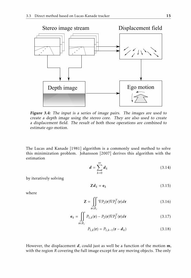
Figure 3.4: The input is a series of image pairs. The images are used tocreate a depth image using the stereo core. They are also used to createa displacement field. The result of both those operations are combined toestimate ego-motion.

The Lucas and Kanade [1981] algorithm is a commonly used method to solvethis minimization problem. Johansson [2007] derives this algorithm with theestimation

d =∞∑k=0

dk (3.14)

by iteratively solving

Zdk = ek (3.15)

where

Z ="r∈Ri

∇P2(r)∇P T2 (r)dr (3.16)

ek ="r∈Ri

P1,k(r) − P2(r)∇P T2 (r)dr (3.17)

P1,k(r) = P1,k−1(r − dk) (3.18)

However, the displacement d, could just as well be a function of the motion m,with the region R covering the full image except for any moving objects. The only

16 3 Ego-motion

change that has to be made to this solution is that the picture gradient

∇P2 =∂P2

∂d=

∂P2

∂(x, y)(3.19)

is extended with the picture gradient with respect to m,

∂P2

∂m=∂d∂m

∂P2

∂d= J∇P2 (3.20)

The new error function

εm ="r∈R

(P2(r + d(r,m)) − P1(r)

)2dr (3.21)

can now be minimized using

Zmmk = em,k (3.22)

where

Zm ="r∈R

ξ(J (r) ·∇P2(r)

)dr, ξ(v) = v · vT (3.23)

em,k ="r∈R

P1,k(r) − P2(r) · J (r) ·∇P T2 (r)dr (3.24)

This result is used in combination with (3.7), augmented for each pixel like (3.9),to produce Algorithm 3.2.

Algorithm 3.2 Direct method1. Calculate a model matrix for how the displacement of each pixel relates to

the rigid motion of the camera based on depth and pixel position, (3.7).2. Calculate weights using (3.11) indicating inlier likelihood for each pixel in

the image.3. Predict the motion for each pixel using previous camera motion and current

depth per pixel.4. Warp the current image towards the previous image based on the predic-

tion.(a) Apply calculated weights.(b) Use gradient descent to find what correction of the motion minimizes

the pictures intensity differences.(c) Iterate.

3.4 Chosen method: Displacement field 17

3.4 Chosen method: Displacement field

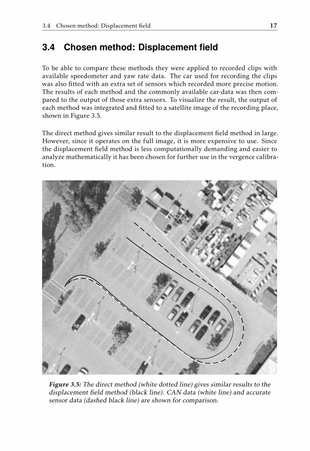
To be able to compare these methods they were applied to recorded clips withavailable speedometer and yaw rate data. The car used for recording the clipswas also fitted with an extra set of sensors which recorded more precise motion.The results of each method and the commonly available car-data was then com-pared to the output of those extra sensors. To visualize the result, the output ofeach method was integrated and fitted to a satellite image of the recording place,shown in Figure 3.5.

The direct method gives similar result to the displacement field method in large.However, since it operates on the full image, it is more expensive to use. Sincethe displacement field method is less computationally demanding and easier toanalyze mathematically it has been chosen for further use in the vergence calibra-tion.

Figure 3.5: The direct method (white dotted line) gives similar results to thedisplacement field method (black line). CAN data (white line) and accuratesensor data (dashed black line) are shown for comparison.

18 3 Ego-motion

3.5 Speed estimation noise sensitivity

For the vergence calibration method described in Chapter 4 to be feasible, thenoise in speed estimation need to be sufficiently bias free, see Section 4.4. In thissection, the noise sensitivity of the chosen method is investigated.

3.5.1 Displacement tracking error

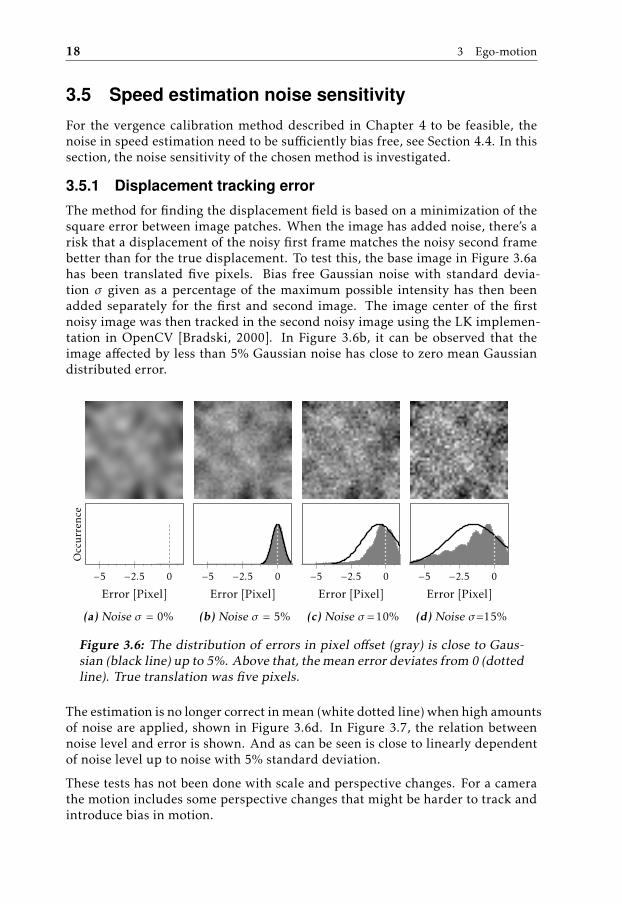
The method for finding the displacement field is based on a minimization of thesquare error between image patches. When the image has added noise, there’s arisk that a displacement of the noisy first frame matches the noisy second framebetter than for the true displacement. To test this, the base image in Figure 3.6ahas been translated five pixels. Bias free Gaussian noise with standard devia-tion σ given as a percentage of the maximum possible intensity has then beenadded separately for the first and second image. The image center of the firstnoisy image was then tracked in the second noisy image using the LK implemen-tation in OpenCV [Bradski, 2000]. In Figure 3.6b, it can be observed that theimage affected by less than 5% Gaussian noise has close to zero mean Gaussiandistributed error.

−5 −2.5 0

Error [Pixel]

Occ

urr

ence

(a) Noise σ = 0%

−5 −2.5 0

Error [Pixel]

(b) Noise σ = 5%

−5 −2.5 0

Error [Pixel]

(c) Noise σ =10%

−5 −2.5 0

Error [Pixel]

(d) Noise σ=15%

Figure 3.6: The distribution of errors in pixel offset (gray) is close to Gaus-sian (black line) up to 5%. Above that, the mean error deviates from 0 (dottedline). True translation was five pixels.

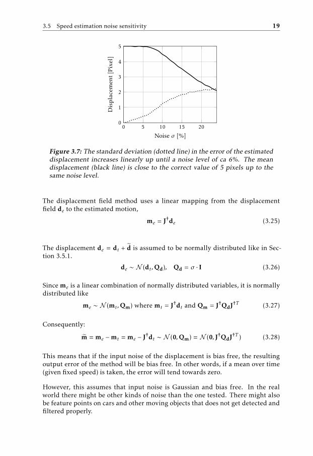
The estimation is no longer correct in mean (white dotted line) when high amountsof noise are applied, shown in Figure 3.6d. In Figure 3.7, the relation betweennoise level and error is shown. And as can be seen is close to linearly dependentof noise level up to noise with 5% standard deviation.

These tests has not been done with scale and perspective changes. For a camerathe motion includes some perspective changes that might be harder to track andintroduce bias in motion.

3.5 Speed estimation noise sensitivity 19

0 5 10 15 200

1

2

3

4

5

Noise σ [%]

Dis

pla

cem

ent

[Pix

el]

Figure 3.7: The standard deviation (dotted line) in the error of the estimateddisplacement increases linearly up until a noise level of ca 6%. The meandisplacement (black line) is close to the correct value of 5 pixels up to thesame noise level.

The displacement field method uses a linear mapping from the displacementfield de to the estimated motion,

me = J†de (3.25)

The displacement de = dt + d is assumed to be normally distributed like in Sec-tion 3.5.1.

de ∼ N (dt ,Qd), Qd = σ · I (3.26)

Since me is a linear combination of normally distributed variables, it is normallydistributed like

me ∼ N (mt ,Qm) where mt = J†dt and Qm = J†QdJ†T (3.27)

Consequently:

m = me −mt = me − J†dt ∼ N (0,Qm) = N (0, J†QdJ†T ) (3.28)

This means that if the input noise of the displacement is bias free, the resultingoutput error of the method will be bias free. In other words, if a mean over time(given fixed speed) is taken, the error will tend towards zero.

However, this assumes that input noise is Gaussian and bias free. In the realworld there might be other kinds of noise than the one tested. There might alsobe feature points on cars and other moving objects that does not get detected andfiltered properly.

20 3 Ego-motion

3.5.2 Depth/disparity estimation error

The depth image is acquired by finding the horizontal displacement (disparity)between the left and the right image for each point. Errors have similar char-acteristics as for the displacement field calculations. At least for a subset of allpoints in the image, the assumption is that disparity is bias free for low amountsof image noise.

It isn’t as simple though, to find out how this affect the ego-motion estimation;this is because the depth is used in the construction of the Jacobian matrix J. TheJacobian matrix is pseudo inverted in the solution m = J†d, which means thatdepth isn’t linearly affecting m.

The method used to analytically determine the effects of displacement noise can’tbe used. Therefore, the problem is analyzed with Monte-Carlo sampling using aspecific test scene. The testing is done using a simulation in Matlab. A pointcloud is made representing a ground surface sampled using a grid pattern likethe one used in Section 3.2.

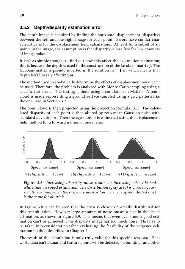
The point cloud is then projected using the projection formula (3.1). The calcu-lated disparity of each point is then altered by zero mean Gaussian noise withstandard deviation σ . Then the ego-motion is estimated using the displacementfield method for a forward motion of one meter.

0.8 0.9 1 1.1

Speed [m/frame]

Occ

urr

ence

(a) Disparity σ = 2 Pixel

0.8 0.9 1 1.1

Speed [m/frame]

(b) Disparity σ = 4 Pixel

0.8 0.9 1 1.1

Speed [m/frame]

(c) Disparity σ = 6 Pixel

Figure 3.8: Increasing disparity noise results in increasing bias (dashedwhite line) in speed estimation. The distribution (gray area) is close to gaus-sian (black line) when the disparity noise is low. The true speed (dotted line)is the same for all trials.

In Figure 3.8 it can be seen that the error is close to normally distributed forthis test situation. However large amounts of noise causes a bias in the speedestimation, as shown in Figure 3.9. This means that even over time, a good esti-mation can’t be achieved if the disparity image has too much noise. This has tobe taken into consideration when evaluating the feasibility of the vergence cali-bration method described in Chapter 4.

The result of this simulation is only truly valid for this specific test case. Realworld data isn’t planar and feature points will be detected on buildings and other

3.5 Speed estimation noise sensitivity 21

0 0.5 1 1.5 20

0.2

0.4

0.6

0.8

1

Disparity error σ [Pixel]

Spee

des

tim

atio

ner

ror

mea

n[%

]

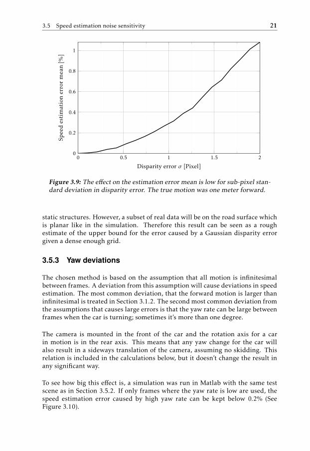
Figure 3.9: The effect on the estimation error mean is low for sub-pixel stan-dard deviation in disparity error. The true motion was one meter forward.

static structures. However, a subset of real data will be on the road surface whichis planar like in the simulation. Therefore this result can be seen as a roughestimate of the upper bound for the error caused by a Gaussian disparity errorgiven a dense enough grid.

3.5.3 Yaw deviations

The chosen method is based on the assumption that all motion is infinitesimalbetween frames. A deviation from this assumption will cause deviations in speedestimation. The most common deviation, that the forward motion is larger thaninfinitesimal is treated in Section 3.1.2. The second most common deviation fromthe assumptions that causes large errors is that the yaw rate can be large betweenframes when the car is turning; sometimes it’s more than one degree.

The camera is mounted in the front of the car and the rotation axis for a carin motion is in the rear axis. This means that any yaw change for the car willalso result in a sideways translation of the camera, assuming no skidding. Thisrelation is included in the calculations below, but it doesn’t change the result inany significant way.

To see how big this effect is, a simulation was run in Matlab with the same testscene as in Section 3.5.2. If only frames where the yaw rate is low are used, thespeed estimation error caused by high yaw rate can be kept below 0.2% (SeeFigure 3.10).

22 3 Ego-motion

−1 −0.5 0 0.5 10

0.1

0.2

0.3

Yaw change per frame [◦]

Est

imat

ion

Err

or[%

]

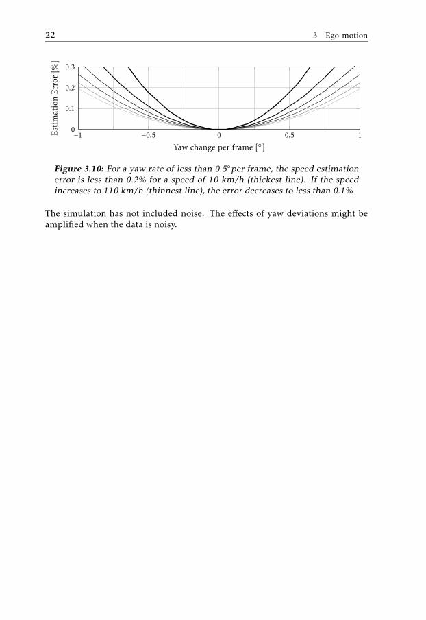
Figure 3.10: For a yaw rate of less than 0.5◦per frame, the speed estimationerror is less than 0.2% for a speed of 10 km/h (thickest line). If the speedincreases to 110 km/h (thinnest line), the error decreases to less than 0.1%

The simulation has not included noise. The effects of yaw deviations might beamplified when the data is noisy.

4Vergence Calibration

This chapter first introduces a potential method for calibrating vergence in shorttime using normal video input, without any special calibration targets. Then therequired components for the method are derived. The noise sensitivity of themethod is analyzed. Finally, the method is evaluated on video recordings withcalibration error introduced manually.

The output of a stereo camera system is dependent on the knowledge of the rela-tive pose between the cameras. There are six degrees of freedom for the relativecamera pose: yaw, pitch, roll, horizontal, vertical and depth axis position. Sincethe cameras in the setup are mounted in a fixed frame, the relative position doesnot change enough to cause significant errors.

However, even a tiny variation in the vergence will cause a significant error indepth estimation and therefore in speed estimation as well (see Figure 4.3b). Thevergence can be calibrated using other methods used at Autoliv, but short term(less than a few minutes) calibration is a problem that isn’t entirely solved. Thischapter introduces one potential solution and tries to determine whether it isfeasible in a real situation.

4.1 Problem definition

The method is based on the fact that an error in vergence angle, shown as γin Figure 4.1, will cause an error in depth. This will then result in an error inspeed estimation. The speedometer information provided by the car is used asreference, and different amounts of vergence compensation are tried in turn. Thevergence angle for which the speed estimation is closest to the true speed is usedas the resulting calibration output. Theoretically, the process can be done with

23

24 4 Vergence Calibration

only two consecutive stereo frame pairs. To reduce noise, it is done for manyframes.

The estimated forward speed, se can be described as a function of vergence errorγ , given two consecutive image pairs,

se = h (γ |Pl1, Pr1, Pl2, Pr2) (4.1)

Given the true speed st , the vergence error is found according to

γ = arg minγ

∣∣st − h(γ)∣∣2 (4.2)

To solve this equation, the function h is sought. The displacement field methodis described using me = J†edt .

1 The only part of Je(γ) that is a function of γ is thedepth Zi(γ) for each point used in the estimation. In the next section, Zi(γ) isderived.

4.2 Estimating depth

As mentioned in Chapter 2, the relation for calculating depth for a calibratedsetup is as simple as Depth = Baseline

Disparity . However, in the scenario of this thesis,the vergence angle is non-zero, so the calibration is incorrect. Therefore, a newexpression is derived.

Bγ

Left

Rightx

z

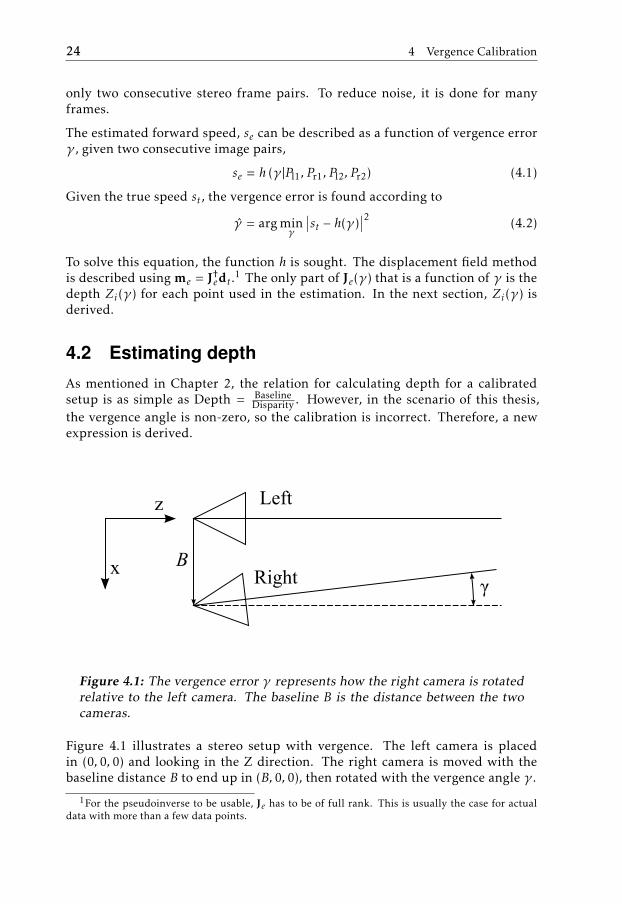
Figure 4.1: The vergence error γ represents how the right camera is rotatedrelative to the left camera. The baseline B is the distance between the twocameras.

Figure 4.1 illustrates a stereo setup with vergence. The left camera is placedin (0, 0, 0) and looking in the Z direction. The right camera is moved with thebaseline distance B to end up in (B, 0, 0), then rotated with the vergence angle γ .

1For the pseudoinverse to be usable, Je has to be of full rank. This is usually the case for actualdata with more than a few data points.

4.3 Vergence estimation algorithm 25

Note: In other related works, left and right vergence are sometimes modeled sep-arately [Brooks et al., 1996]. Modeling the angles separately makes calculationslonger and the difference can just as well be described as a difference in z-positionbetween the cameras. For small angles, the z-component would be insignificantcompared to the x-component. To make calculations more compact, the vergenceangle is modeled only for the right camera in this thesis.

Since stereo separation can be seen as a horizontal camera motion, the motionrelation from Section 3.1.1 is reused. So the relation between vergence and stereoestimated depth Z(γ) is found using (3.6) with ∆xi seen as the disparity. Elimi-nating all rotation but vergence wy = γ and all translation but baseline tx = Bgives the expression

∆xi(γ) = xi −cos γ (xi Zi − B) + sin γ Zicos γ Zi − sin γ (xi Zi − B)

(4.3)

This equation can be solved to extract depth as a function of vergence error

Zi(γ) =(sin γ xi − ∆xi sin γ + cos γ) B

sin γ x2i − ∆xi sin γ xi + sin γ + ∆xi cos γ

(4.4)

4.3 Vergence estimation algorithm

The equation (4.2) is numerically solved in Algorithm 4.1 using a grid search. Theestimated speed function h(γ) is calculated using the displacement field methodwith the depth replaced with (4.4).

Algorithm 4.1 Vergence calibration algorithm• For each frame in a clip:

– Estimate motion me given a series of vergences, γ1, γ2, ..., γm.– If the motion is forward, (Yaw < Yaw0) (see Section 3.5.3)* Find for which vergences the difference between true and esti-

mated speed changes sign.* Add those vergences to the set Γ of estimated vergences.

• Return the mode of Γ as the estimated vergence.

If there is more than one minima of the error function, all are used to be sure tonot miss the correct alternative. The basis of the error function, st − h(γ), shouldcross zero if the true error is within the range and no errors occurs. This meansthat the minima of the error function will be when st − h(γ) crosses zero, i.e.where it changes sign between two consecutive γi .

In Section 3.5 the effects of bias free Gaussian displacement noise are found tobe zero mean in speed estimation. As long as the errors are reasonably low, thelong time mean value of estimations of a given static speed will be accurate. Thiswould mean that the mean value of the estimated vergence error per frame pairshould be correct.

26 4 Vergence Calibration

However, this is based on an assumption of no outliers and trials with the meandoes not perform well as seen in Figure 4.2a. Using the median is often a goodway to reduce the effect of outliers. However, the median only works if the out-liers aren’t too many and biased in any way. As Figure 4.2b shows, using themedian does give a slight improvement; the estimation is still quite off.

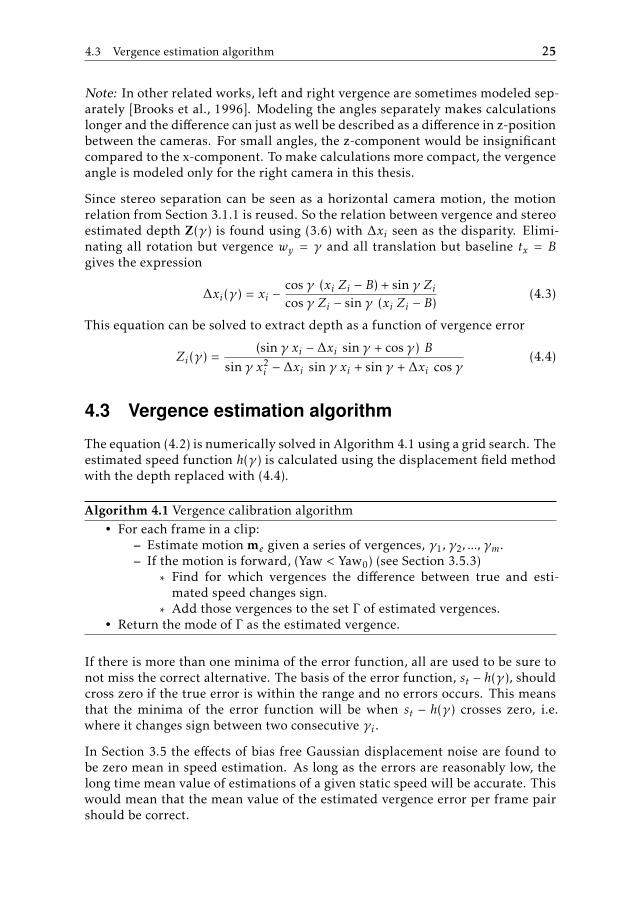
To improve this, a histogram of estimated vergences is created, and the peakingvalue, the mode, is used. The results shown in Figure 4.2c are close to the truevalue. If the vergences are estimated to arbitrary precision the histogram needsto be filtered in some way. In the trials done here the histogram is quantized to0.025◦precision which is enough to create a clear peak in the data for the data setused in these trials.

−0.1◦ 0◦ 0.1◦0

1

2

3

Vergence error

Cou

nt

0.00◦

(a) Method: mean

−0.1◦ 0◦ 0.1◦0

1

2

3

Vergence error

0.00◦

(b) Method: median

−0.01◦ 0◦ 0.01◦0246

Vergence error

0.00◦

(c) Method: mode

Figure 4.2: The resulting vergence estimations for a number of 30-secondclips with 0.00 ± 0.005◦error are shown. Three statistical methods are usedto estimate vergence based on all per-frame estimations in the clip. Usingthe mode of the estimations yields results closest to the true value

4.4 Speed estimation vergence sensitivity

For this method to be usable in real traffic situations, the effects of vergence errorhas to be greater than the effects of other error sources like noise. The speedestimation error caused by a change in vergence of the same size as the desiredprecision in the vergence estimation needs to be greater than the speed estimationerror caused by other factors.

In Chapter 3 the effects of noise and yaw error on speed estimation are inves-tigated. If the results shown in Figure 3.7 and Figure 3.9 are combined, it canbe inferred that for image noise with standard deviation σ = 5% the speed esti-mation error is around 0.1%. If the image noise is increased to 15% the speedestimation error increases to around 1%.

Section 3.5.3 continues to investigate the effects of the car steering on the speedestimation error due to approximation. As long as yaw is kept low, the errorcaused by steering should be less than 0.2%.

If the error caused by noise and yaw rate are added, an error of between 0.3% and0.12% could be expected. Since 15% image noise is more than seen in actual data,

4.5 Vergence error calibration method 27

an expected error in the lower end of the scale, 0.5% has been used in furtheranalysis.

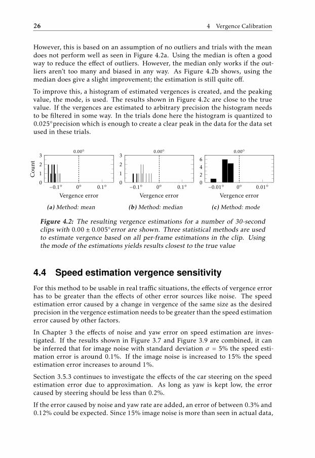
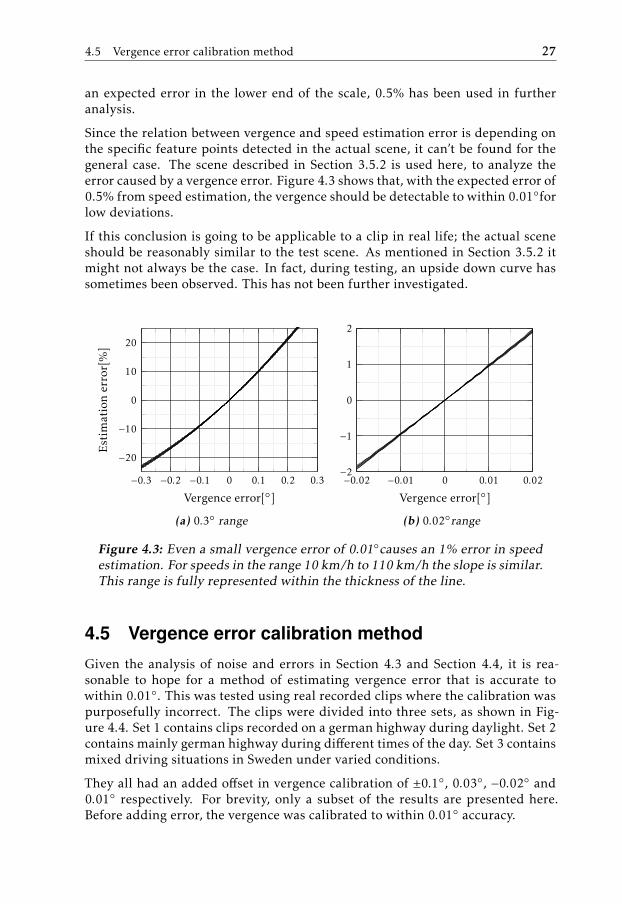
Since the relation between vergence and speed estimation error is depending onthe specific feature points detected in the actual scene, it can’t be found for thegeneral case. The scene described in Section 3.5.2 is used here, to analyze theerror caused by a vergence error. Figure 4.3 shows that, with the expected error of0.5% from speed estimation, the vergence should be detectable to within 0.01◦forlow deviations.

If this conclusion is going to be applicable to a clip in real life; the actual sceneshould be reasonably similar to the test scene. As mentioned in Section 3.5.2 itmight not always be the case. In fact, during testing, an upside down curve hassometimes been observed. This has not been further investigated.

−0.3 −0.2 −0.1 0 0.1 0.2 0.3

−20

−10

0

10

20

Vergence error[◦]

Est

imat

ion

erro

r[%

]

(a) 0.3◦ range

−0.02 −0.01 0 0.01 0.02−2

−1

0

1

2

Vergence error[◦]

(b) 0.02◦range

Figure 4.3: Even a small vergence error of 0.01◦causes an 1% error in speedestimation. For speeds in the range 10 km/h to 110 km/h the slope is similar.This range is fully represented within the thickness of the line.

4.5 Vergence error calibration method

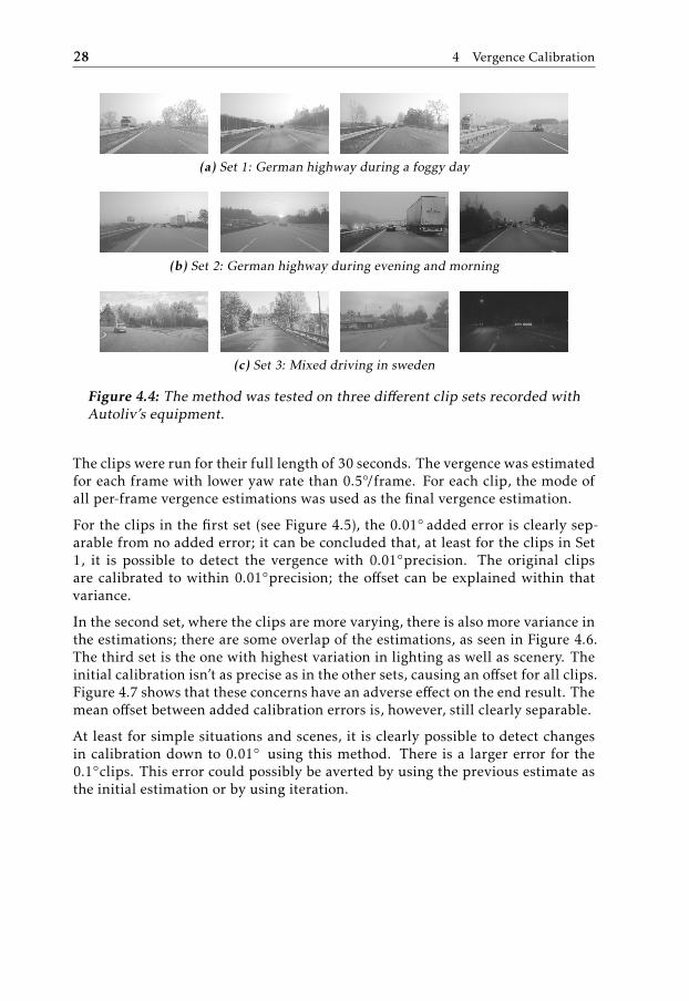
Given the analysis of noise and errors in Section 4.3 and Section 4.4, it is rea-sonable to hope for a method of estimating vergence error that is accurate towithin 0.01◦. This was tested using real recorded clips where the calibration waspurposefully incorrect. The clips were divided into three sets, as shown in Fig-ure 4.4. Set 1 contains clips recorded on a german highway during daylight. Set 2contains mainly german highway during different times of the day. Set 3 containsmixed driving situations in Sweden under varied conditions.

They all had an added offset in vergence calibration of ±0.1◦, 0.03◦, −0.02◦ and0.01◦ respectively. For brevity, only a subset of the results are presented here.Before adding error, the vergence was calibrated to within 0.01◦ accuracy.

28 4 Vergence Calibration

(a) Set 1: German highway during a foggy day

(b) Set 2: German highway during evening and morning

(c) Set 3: Mixed driving in sweden

Figure 4.4: The method was tested on three different clip sets recorded withAutoliv’s equipment.

The clips were run for their full length of 30 seconds. The vergence was estimatedfor each frame with lower yaw rate than 0.5◦/frame. For each clip, the mode ofall per-frame vergence estimations was used as the final vergence estimation.

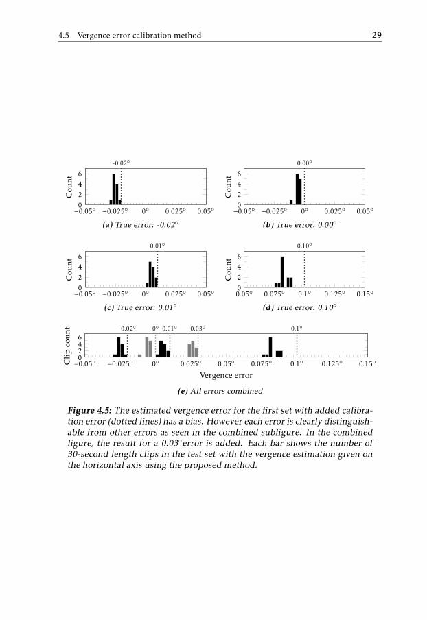
For the clips in the first set (see Figure 4.5), the 0.01◦ added error is clearly sep-arable from no added error; it can be concluded that, at least for the clips in Set1, it is possible to detect the vergence with 0.01◦precision. The original clipsare calibrated to within 0.01◦precision; the offset can be explained within thatvariance.

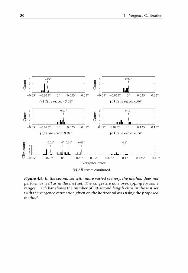
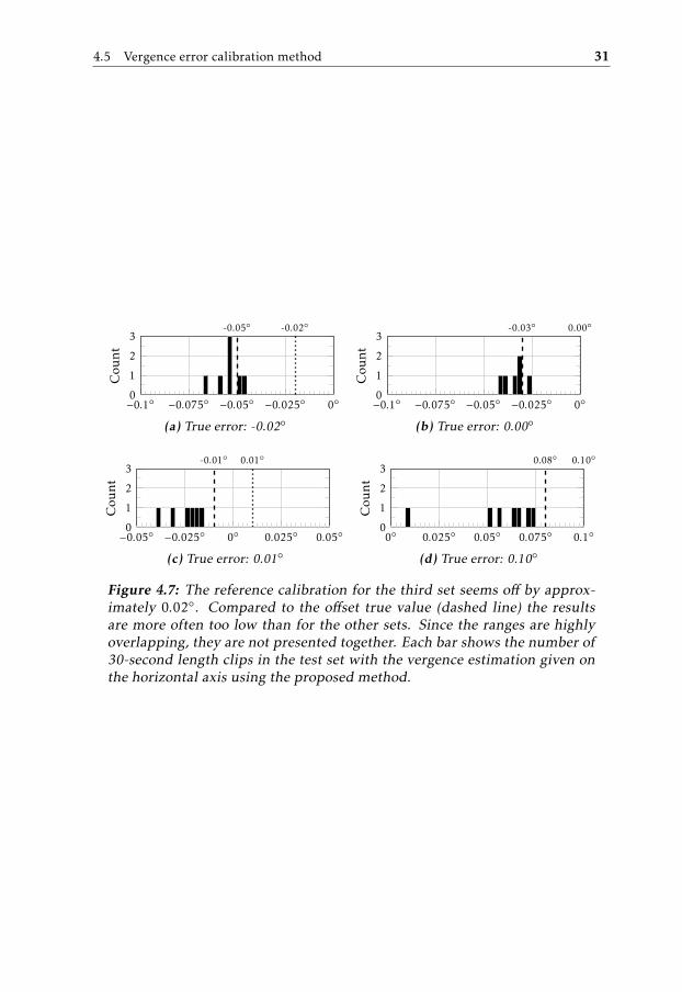
In the second set, where the clips are more varying, there is also more variance inthe estimations; there are some overlap of the estimations, as seen in Figure 4.6.The third set is the one with highest variation in lighting as well as scenery. Theinitial calibration isn’t as precise as in the other sets, causing an offset for all clips.Figure 4.7 shows that these concerns have an adverse effect on the end result. Themean offset between added calibration errors is, however, still clearly separable.

At least for simple situations and scenes, it is clearly possible to detect changesin calibration down to 0.01◦ using this method. There is a larger error for the0.1◦clips. This error could possibly be averted by using the previous estimate asthe initial estimation or by using iteration.

4.5 Vergence error calibration method 29

−0.05◦ −0.025◦ 0◦ 0.025◦ 0.05◦0246

Cou

nt

-0.02◦

(a) True error: -0.02◦−0.05◦ −0.025◦ 0◦ 0.025◦ 0.05◦

0246

Cou

nt

0.00◦

(b) True error: 0.00◦

−0.05◦ −0.025◦ 0◦ 0.025◦ 0.05◦0246

Cou

nt

0.01◦

(c) True error: 0.01◦0.05◦ 0.075◦ 0.1◦ 0.125◦ 0.15◦0246

Cou

nt

0.10◦

(d) True error: 0.10◦

−0.05◦ −0.025◦ 0◦ 0.025◦ 0.05◦ 0.075◦ 0.1◦ 0.125◦ 0.15◦0246

Vergence error

Cli

pco

unt -0.02◦ 0◦ 0.01◦ 0.03◦ 0.1◦

(e) All errors combined

Figure 4.5: The estimated vergence error for the first set with added calibra-tion error (dotted lines) has a bias. However each error is clearly distinguish-able from other errors as seen in the combined subfigure. In the combinedfigure, the result for a 0.03◦error is added. Each bar shows the number of30-second length clips in the test set with the vergence estimation given onthe horizontal axis using the proposed method.

30 4 Vergence Calibration

−0.05◦ −0.025◦ 0◦ 0.025◦ 0.05◦0246

Cou

nt

-0.02◦

(a) True error: -0.02◦−0.05◦ −0.025◦ 0◦ 0.025◦ 0.05◦

0246

Cou

nt

0.00◦

(b) True error: 0.00◦

−0.05◦ −0.025◦ 0◦ 0.025◦ 0.05◦0246

Cou

nt

0.01◦

(c) True error: 0.01◦0.05◦ 0.075◦ 0.1◦ 0.125◦ 0.15◦0246

Cou

nt

0.10◦

(d) True error: 0.10◦

−0.05◦ −0.025◦ 0◦ 0.025◦ 0.05◦ 0.075◦ 0.1◦ 0.125◦ 0.15◦0246

Vergence error

Cli

pco

unt -0.02◦ 0◦ 0.01◦ 0.03◦ 0.1◦

(e) All errors combined

Figure 4.6: In the second set with more varied scenery, the method does notperform as well as in the first set. The ranges are now overlapping for someranges. Each bar shows the number of 30-second length clips in the test setwith the vergence estimation given on the horizontal axis using the proposedmethod.

4.5 Vergence error calibration method 31

−0.1◦ −0.075◦ −0.05◦ −0.025◦ 0◦0

1

2

3

Cou

nt

-0.02◦-0.05◦

(a) True error: -0.02◦−0.1◦ −0.075◦ −0.05◦ −0.025◦ 0◦0

1

2

3

Cou

nt

0.00◦-0.03◦

(b) True error: 0.00◦

−0.05◦ −0.025◦ 0◦ 0.025◦ 0.05◦0

1

2

3

Cou

nt

0.01◦-0.01◦

(c) True error: 0.01◦0◦ 0.025◦ 0.05◦ 0.075◦ 0.1◦

0

1

2

3

Cou

nt

0.10◦0.08◦

(d) True error: 0.10◦

Figure 4.7: The reference calibration for the third set seems off by approx-imately 0.02◦. Compared to the offset true value (dashed line) the resultsare more often too low than for the other sets. Since the ranges are highlyoverlapping, they are not presented together. Each bar shows the number of30-second length clips in the test set with the vergence estimation given onthe horizontal axis using the proposed method.

5Concluding remarks

In this chapter a concluding summary of the thesis is given and ideas for futurework on the method are presented.

5.1 Conclusion

In Chapter 3, a method for estimating visual odometry is sought. Two methodsare derived, the displacement field method and the gradient descent method. Thedisplacement field method is chosen due to lower computational demand and thefact that it has adequate precision compared to the more costly gradient descentmethod.

Chapter 4 introduces a method for calibration of vergence angle. It uses a combi-nation of visual odometry, from Chapter 3, and mechanical odometry, from thespeedometer in the car. According to estimations in Chapter 4, it is feasible to getaccurate results at least to within 0.01◦ precision.

The method is implemented in Autoliv’s framework and tested on clips providedby Autoliv. The results from two of the sets have a bias error of approximately0.005◦ that could be explained by an error in the provided ground truth calibra-tion. It is found that, at least for simple situations and scenes, it is clearly possibleto detect changes in calibration down to 0.01◦ using the evaluated method.

5.2 Future work

The tests has a bias in estimation, this is most likely due to calibration errors inthe source material. The method could be tested on clips with an error of less

33

34 5 Concluding remarks

than 0.001◦ for a more accurate estimation of the precision in mean. In the 0.1◦

clip the error is larger than the bias, this might be due to approximation errors.The approximation errors due to linearization should be analyzed and a solutionfor large error calibration should be sought. An iterative solution would probablysolve the problem, albeit with a computational cost.

In Section 4.4, a discrepancy between the model and real data is briefly men-tioned. This should be investigated further and the reason should be identified.

The described method estimates the speed given all possible vergence errors. Thisis computationally expensive; it might be possible to reduce the vergence estima-tion step to a single expression rather than an iteration procedure. This couldeither be done by restricting the movement for a frame to only forward motion,or by analytically finding the relation between speed error and vergence errorbased on a given set of feature points.

The accuracy of the solution is dependent on the accuracy of the speed estimation.The direct method described in Section 3.3 could possibly be extended to directlygive the vergence error. This could reduce the number of intermediate steps andimprove the estimation result.

For more accurate reliability data, a much larger data set should be used. Prob-lems caused by peculiar situations should then be solved as they are found.

Bibliography

Gilad Adiv. Determining three-dimensional motion and structure from opticalflow generated by several moving objects. Pattern Analysis and Machine Intel-ligence, IEEE Transactions on, PAMI-7(4):384 –401, july 1985. ISSN 0162-8828.doi: 10.1109/TPAMI.1985.4767678. Cited on pages 2 and 12.

G. Bradski. The OpenCV Library. Dr. Dobb’s Journal of Software Tools, 2000.Cited on pages 13 and 18.

M. J. Brooks, L. Agapito, D. Q. Huynh, and L. Baumela. Direct methods forself-calibration of a moving stereo head. In Proc. European Conference onComputer Vision, pages 415–426. Springer, 1996. Cited on pages 3 and 25.

C. Golban and S. Nedevschi. Linear vs. non linear minimization in stereo visualodometry. In Intelligent Vehicles Symposium (IV), 2011 IEEE, pages 888 –894,june 2011. doi: 10.1109/IVS.2011.5940537. Cited on page 2.

K.J. Hanna. Direct multi-resolution estimation of ego-motion and structure frommotion. In Visual Motion, 1991., Proceedings of the IEEE Workshop on, pages156 –162, oct 1991. doi: 10.1109/WVM.1991.212812. Cited on pages 12and 14.

R. Horaud, G. Csurka, and D. Demirdijian. Stereo calibration from rigid motions.Pattern Analysis and Machine Intelligence, IEEE Transactions on, 22(12):1446–1452, dec 2000. ISSN 0162-8828. doi: 10.1109/34.895977. Cited on page 3.

J. Horn, A. Bachmann, and Thao Dang. Stereo vision based ego-motion estima-tion with sensor supported subset validation. In Intelligent Vehicles Sympo-sium, 2007 IEEE, pages 741 –748, june 2007. doi: 10.1109/IVS.2007.4290205.Cited on page 12.

M. Irani, B. Rousso, and S. Peleg. Recovery of ego-motion using image stabiliza-tion. In Computer Vision and Pattern Recognition, 1994. Proceedings CVPR’94., 1994 IEEE Computer Society Conference on, pages 454 –460, jun 1994.doi: 10.1109/CVPR.1994.323866. Cited on pages 2 and 12.

M. Irani, B. Rousso, and S. Peleg. Recovery of ego-motion using region alignment.

35

36 Bibliography

Pattern Analysis and Machine Intelligence, IEEE Transactions on, 19(3):268 –272, mar 1997. ISSN 0162-8828. doi: 10.1109/34.584105. Cited on page 2.

B Johansson. Derivation of lucas-kanade tracker, November 2007. URL http://www.cvl.isy.liu.se/education/graduate/undergraduate/tsbb12/reading-material/LK-derivation.pdf. Cited on page 15.

H. C. Longuet-Higgins and K. Prazdny. The interpretation of a moving retinal im-age. Proceedings of the Royal Society of London. Series B. Biological Sciences,208(1173):385–397, 1980. doi: 10.1098/rspb.1980.0057. Cited on page 2.

B.D. Lucas and T. Kanade. An iterative image registration technique with anapplication to stereo vision. In Proceedings of the 7th international joint con-ference on Artificial intelligence, 1981. Cited on pages 13 and 15.

G.P. Stein, O. Mano, and A. Shashua. A robust method for computing vehicle ego-motion. In Intelligent Vehicles Symposium, 2000. IV 2000. Proceedings of theIEEE, pages 362 –368, 2000. doi: 10.1109/IVS.2000.898370. Cited on pages 12and 13.

Zhengyou Zhang. Flexible camera calibration by viewing a plane from unknownorientations. In Computer Vision, 1999. The Proceedings of the Seventh IEEEInternational Conference on, volume 1, pages 666 –673 vol.1, 1999. doi: 10.1109/ICCV.1999.791289. Cited on page 2.

Upphovsrätt

Detta dokument hålls tillgängligt på Internet — eller dess framtida ersättare —under 25 år från publiceringsdatum under förutsättning att inga extraordinäraomständigheter uppstår.

Tillgång till dokumentet innebär tillstånd för var och en att läsa, ladda ner,skriva ut enstaka kopior för enskilt bruk och att använda det oförändrat för icke-kommersiell forskning och för undervisning. Överföring av upphovsrätten viden senare tidpunkt kan inte upphäva detta tillstånd. All annan användning avdokumentet kräver upphovsmannens medgivande. För att garantera äktheten,säkerheten och tillgängligheten finns det lösningar av teknisk och administrativart.

Upphovsmannens ideella rätt innefattar rätt att bli nämnd som upphovsmani den omfattning som god sed kräver vid användning av dokumentet på ovanbeskrivna sätt samt skydd mot att dokumentet ändras eller presenteras i sådanform eller i sådant sammanhang som är kränkande för upphovsmannens litteräraeller konstnärliga anseende eller egenart.

För ytterligare information om Linköping University Electronic Press se förla-gets hemsida http://www.ep.liu.se/

Copyright

The publishers will keep this document online on the Internet — or its possi-ble replacement — for a period of 25 years from the date of publication barringexceptional circumstances.

The online availability of the document implies a permanent permission foranyone to read, to download, to print out single copies for his/her own use andto use it unchanged for any non-commercial research and educational purpose.Subsequent transfers of copyright cannot revoke this permission. All other usesof the document are conditional on the consent of the copyright owner. Thepublisher has taken technical and administrative measures to assure authenticity,security and accessibility.

According to intellectual property law the author has the right to be men-tioned when his/her work is accessed as described above and to be protectedagainst infringement.

For additional information about the Linköping University Electronic Pressand its procedures for publication and for assurance of document integrity, pleaserefer to its www home page: http://www.ep.liu.se/

© Sebastian Jansson