Institute of Water Resources Annual Technical Report

FY 2002

IntroductionIn fiscal year 2002, the Connecticut Institute of Water Resources continued to be administered by Dr.Glenn Warner, Director, and Dr. Patricia Bresnahan, Associate Director, both in the Department ofNatural Resource Management and Engineering, in teh College of Agriculture and Natural Resources atthe University of Connecticut.

While located at the University of Connecticut, the Institute’s mission is to cooperate closely with allcolleges and universities in teh state to resolve state and regional water related problems and provide astrong connection between water resource managers and teh academic community. CT IWR responds toenvironmental issues in Connectcut througha statewide Advisory Board and through its involvement withstate water resource committees. Membership reflects the main constituency groups for the Institute:government agencies, environmental groups, the water industry and academic researchers.

Research ProgramEach year, the Connecticut Institute conducts a competitive RFP process to solicit proposals for fundingunder the USGS 104B program. Announcements are sent to every water resource related academicprogram in the state. Proposals received are sent out for peer review, and a furthere technical review isconducted by members of the CT IWR Advisory Board and others with relevant technical expertise. TheAdvisory Board then reviews teh relevance of the proposals to state water research needs, and makesfunding recommendations to the Institute Director.

This year, two research projects were selected for funding:

"Water Quality Assessment in Connecticut: Evaluation of Current Protocols and Development ofImproved Methods." Shimone Anisfeld, Yale University.

"Development of Regionally Callibrated Land Cover Impervious Surface Coefficients." Michael Prisloeand Dan Civco, University of Connecticut.

In addition to its 104B research projects, the CT IWR is administering the Fenton River Aquatic Study forthe Univ. of CT, Department of Facilities. The project began November 1, 2002 and is scheduled to endDecember 31, 2004. The purpose of the study is to determine the potential impacts of withdrawals fromthe UConn water supply wells that lie in the floodplain of the Fenton river on the flow and fisheries habitatin the Fenton. There are three components to the study: surface water flow in the Fenton and its tributaries,ground water levels at different levels and positions and fisheries habitat and fish use of the Fenton. Thestudy team consists of Fred Ogden (Civil and Environmental Engr.), George Hoag (Civil andEnvironmental Engr.), Glenn Warner (Natural Resources Management and Engineering), Jeff Starn(USGS) and Piotr Parasiewcisz (Cornell) and Rick Jacobson (Natural Resources Management andEngineering). The interactions of surface-ground water will be measured and mathematically modeled at

different water levels. Fish habitat and fish use will be monitored and used to develop a PHABSIM model.Total study cost is $ 571,089. A Technical Advisory Group consisting of representatives from State andFederal agencies and environmental groups provides technical input to the study.

Water Quality Assessment in Connecticut: Evaluation ofCurrent Protocols and Development of Improved Methods

Basic Information

Title:Water Quality Assessment in Connecticut: Evaluation of Current Protocols andDevelopment of Improved Methods

Project Number: 2002CT2B

Start Date: 3/1/2002

End Date: 2/28/2003

Funding Source: 104B

Congressional District:

3rd

Research Category: Not Applicable

Focus Category: Non Point Pollution, Surface Water, Water Quality

Descriptors: Bacteria, Suspended Sediments, Water Quality Monitoring

Principal Investigators:

Shimon Anisfeld, Shimon Anisfeld

Publication

Title:

Water Quality Assessment in Connecticut: Evaluation of Current Protocols and Development of Improved Methods

Focus Categories: Nonpoint Pollution, Surface Water, Water Quality Keywords: Bacteria, Nitrogen, Trace Metals, Water Quality Monitoring Duration: March 1, 2002 – February 28, 2003 Principal Investigator: Shimon Anisfeld, Yale School of Forestry & Environmental Studies Congressional District: 3rd Statement of Critical Regional or State Water Problem

Connecticut relies on a water quality monitoring program to assess whether state water bodies (e.g., streams and rivers) are meeting water quality standards and supporting their designated uses. This monitoring program is faced with a task both important and difficult: important because of the significant costs and consequences associated with incorrectly listing (or not listing) a water body as impaired; and difficult because of the high temporal and spatial variability in stream water quality, and the limited resources available for assessing large numbers of water bodies. The task of accurate water quality assessment can be made easier by a better understanding of temporal variability and how it affects the results obtained from a limited set of samples.

We propose to carry out pilot research to evaluate how temporal variability in stream conditions affects the results of Connecticut’s current water quality assessment program. This research will also be useful more broadly in aiding in the interpretation of water quality measurements taken at infrequent intervals. The underlying question that we hope to address is: Given a limited set of measurements of pollutant concentration in a stream, how much can one say about concentrations of that pollutant during unsampled periods? Specific questions that derive from this overall objective are the following: • Given Connecticut’s current sampling scheme, what are the probabilities of making type I and

type II errors? • Given a set of concentration measurements at specific points in time, what is the uncertainty

associated with extrapolating these measurements to other times? • How many samples must be taken in order to reduce this uncertainty to an acceptable level? • Can the number of samples required be reduced by careful choice of sampling timing (e.g.,

making sure to cover different flow conditions)?

Statement of Results or Benefits

Our proposal involves collection of a temporally-intensive data set (~200 samples at one site over a 4 month period) to delineate the seasonal, flow-associated, and random variability in levels of bacterial indicators (E. coli, fecal coliform), nitrogen, and trace metals. The proposed site is at the USGS gauging station on the Quinnipiac River in Wallingford, where both streamflow (near-real-time) and water quality data (8 times/year) are available from the USGS. We will compare the use support results and other summary measures obtained from the complete data set to those obtained from subsets of the data. These subsets will be derived from Monte Carlo sampling and will mimic different sampling frequencies (e.g., the 8-12 samples per year associated with the current monitoring scheme). This will allow us to begin to answer the questions outlined above.

Results from this project (and a subsequent, larger research program) will allow CT DEP (and other agencies) to redesign its monitoring programs to obtain the greatest amount of water quality information for the lowest cost. Our results will help provide a clearer picture of the health of the state’s streams. They will help to prevent costly errors in the state’s list of impaired water bodies, and will ultimately help the state direct its resources to those water bodies in greatest need of protection and restoration. They will also be useful in gaining a better estimate of nitrogen loading to Long Island Sound and a fuller understanding of what sampling frequency is required for accurate assessment of nitrogen loading to the Sound from Connecticut rivers.

Nature, Scope, and Objectives

There is a general need for accurate, cost-effective methods of assessing the health of aquatic ecosystems. For example, Section 305(b) of the Clean Water Act requires states to regularly assess whether the state’s waters (rivers, lakes, and estuaries) are meeting state wate r quality standards (WQS). Typically, the resources available for this task are small in comparison to the large number of water bodies for which assessments are required. However, stakes are high: mistaken listing of a water body as impaired (not meeting WQS) can activate the expensive total maximum daily load (TMDL) process for no reason, while a mistaken declaration that a water body is supporting all uses (i.e., meeting WQS) will divert attention from cleaning it up.

The task of assessing riverine health is further complicated by the highly dynamic nature of these ecosystems. The fact that conditions can change quickly in both time and space means that a full assessment of water quality requires a prohibitively large number of samples. Understanding the spatial and temporal variability in water quality is essential for an accurate assessment of whether a given stream meets water quality standards.

The Connecticut Department of Environmental Protection (CT DEP) relies increasingly on biological monitoring for its assessments, in large part as a way of dealing with temporal variability in stream water quality (Connecticut Department of Environmental Protection 1999). Biological monitoring presumably integrates the effects of water quality over a relatively long period of time (weeks to months), so that it may give a more accurate reflection of whether water quality is limiting to the biological community than would a small set of water chemistry measurements made at specific points in time. However, biological monitoring has several shortcomings, including our limited understanding of the relationship between water chemistry and biotic health, and difficulties in interpretation of results, especially when an adequate reference site does not exist. In addition, biological monitoring is restricted to assessment of aquatic life use support, not of other uses. Thus, for example, a stream with a healthy macroinvertebrate community could be regularly violating WQS for indicator bacteria (a standard based on protecting human health, not aquatic life support).

In its direct assessments of water quality (i.e., those not based on biotic monitoring), CT DEP relies on three types of monitoring programs: • a long-standing cooperative program with the USGS, in which 33 sites throughout the state

(mostly on large, waste-receiving rivers) are sampled 8-12 times per year; • a rotating basin program, in which a different basin is selected each year for spatially intensive

sampling; samples are collected from these sites 4 times per year (Connecticut Department of Environmental Protection 1999);

• intensive water quality surveys of specific watersheds. (DEP also analyzes fish tissue samples for toxic bioaccumulative compounds.) Because of the limited budgets and consequently small sample numbers collected per site, these programs – with the exception of the intensive water quality surveys – are very limited in their ability to delineate the temporal variability in water quality.

EPA guidance acknowledges the role of temporal variability by permitting a certain fraction of the samples taken at a particular site to be above WQS before requiring the site to be listed as

impaired (e.g., for temperature standards for aquatic life use support, the site can be considered fully supporting if up to 10% of measurements exceed the standard (US Environmental Protection Agency 1997)).

However, the small number of samples currently used for assessment may greatly increase the chances of either: • a type I error: a site is declared im paired when it is not (i.e., the samples happened to be

taken under unusually bad conditions); or • a type II error: a site is declared healthy when it is in fact impaired (i.e., the samples happened

to be taken under unusually good conditions).

We propose to carry out pilot research to evaluate how temporal variability in stream conditions affects the results of Connecticut’s current water quality assessment program. This research will also be useful more broadly in aiding in the interpretation of water quality measurements taken at infrequent intervals. The underlying question that we hope to address is: Given a limited set of measurements of pollutant concentration in a stream, how much can one say about concentrations of that pollutant during unsampled periods?

Specific questions that derive from this overall objective are the following:

• Given the current sampling scheme, what are the probabilities of making type I and type II

errors? • Given a set of concentration measurements at specific points in time, what is the uncertainty

associated with extrapolating these measurements to other times? • How many samples must be taken in order to reduce this uncertainty to an acceptable level? • Can the number of samples required be reduced by careful choice of sampling timing (e.g.,

making sure to cover different flow conditions)? Note that the answer to the first question clearly depends on the measured concentrations: If these greatly exceed WQS on the sampling dates, then it is very likely that the stream is truly impaired, while if measurements exceed WQS only slightly or not on all dates, then the true impairment status of the stream may be more difficult to ascertain. We hope to use the answer to question 2 (an estimate of the uncertainty associated with extrapolation of a given set of measurements) to provide managers with the tools to quantitate the probability of type I and II errors in specific situations.

We will focus our analysis on three types of water quality parameters, namely, indicator bacteria, nitrogen, and trace metals, for three reasons: • these parameters are not captured well by biological monitoring; • temporal variability tends to be particularly high for these parameters (e.g., in response to

storm events); • current assessment techniques have found many CT rivers to be in violation of WQS for

bacteria: the 2000 305(b) report found indicator bacteria impairment for 67 out of 194 segments representing 239 out of 673 miles of river (Connecticut Department of Environmental Protection 2000);

• the accuracy of estimates of N loading to Long Island Sound from Connecticut watersheds is dependent on the uncertainty associated with extrapolating from limited sampling dates.

Connecticut is currently in transition from a reliance on fecal coliform as an indicator of the possibility of pathogen contamination to the use of E. coli, a more accurate indicator of the potential for human health effects. Samples collected by the USGS are analyzed for fecal coliform and enterococci, but not E. coli. We will analyze our samples both for E. coli (for comparison to the new water quality standard) and for fecal coliform (for comparison to USGS data). Methods, Procedures and Facilities Approach: Our approach to answering the questions outlined above involves collection of a temporally-intensive data set on E. coli, fecal coliform, nitrogen, and trace metal levels, followed by comparison of this data set to the more limited data collection typical of DEP and USGS sampling in Connecticut. This will be done at one site: the USGS gauging station on the Quinnipiac River in Wallingford. The streamflow data that we need for data analysis (and for determining sample collection timing; see below) is available on a near-real-time basis for this site from the USGS. In addition, the USGS collects 8 water quality samples per year at this site, which will serve as the basis for our comparison. Generally, four of these samples are collected during the summer (monthly, June-September), while the other four samples are collected during the remainder of the year (semi-monthly, October-May). As a pilot project, our sampling will be limited to June-September (which is the period of greatest concern, especially over bacteria levels). Sample collection and analysis: The proposed frequency of sample collection is limited by the fact that samples must be collected manually (due to the need for sterile sampling and the short holding time for analysis of fecal coliform and E. coli). However, sample collection would take place at a frequency sufficient to capture the great majority of the seasonal and flow-induced variability in conditions during the summer months. Specifically, we envision the following sample collection scheme:

• baseflow samples collected every 3 days (total over 4 months = 40 samples); • stormflow samples collected over the course of every stormflow event during these 4

months (total = ~20 samples/storm x ~8 storms = ~160 samples), as follows: o rising limb: samples collected every 3 hours from the beginning of the

stormflow event until 3 hours after the peak in streamflow o falling limb I: samples collected every 6 hours until the point at which flow has

fallen 50% of the way to pre-storm levels o falling limb II: samples collected every 12 hours until the point at which flow

has fallen 75% of the way to pre-storm levels. o Note: For these purposes, we will consider a stormflow event to commence

when 0.5 in of rain have fallen within a 24-hour period (recorded at a rain gauge near Greeley Laboratory, New Haven).

The “complete” data set at this site will thus consist of a total of ~200 samples over a 4 month period (not including QA samples; see below). In addition, twice during these 4 months, we will collect baseflow samples every 3 hours over a 24 hour period, in order to assess the diurnal and random variability in concentrations during baseflow. Grab samples will be collected for analysis of E. coli, fecal coliform, nitrogen, and trace metals. Samples will be collected and analyzed using standard techniques (Clesceri et al. 1999). Three grab samples will be collected. The first, collected into a sterile sample bottle, will be returned to the laboratory and analyzed for E. coli and fecal coliform using the standard EPA membrane filtration methods (US Environmental Protection Agency 2000). The second sample bottle will be filtered in the field using trace metal “clean techniques,” while the third sample will be a raw (unfiltered) sample collected using clean techniques (Benoit 1994). These sample bottles will be returned to the laboratory, where an aliquot from the raw sample will be frozen for later analysis of nitrogen. The remainder of the raw and filtered samples will be acidified and stored in the refrigerator for later analysis of trace metals. Nitrogen samples will be thawed within 30 days of collection and analyzed for NO3

- (ion chromatography; Clesceri et al. 1999) and total N (alkaline persulfate digestion, followed by ion chromatography; D’Elia et al. 1977). Both raw and filtered trace metal samples will be concentrated by evaporative concentration within 90 days of collection and analyzed for Pb, Ag, Cu, and Cd by graphite furnace atomic absorption spectoscopy. All of these measurements are familiar to the PI and are routinely carried out in our laboratory. Careful attention will be paid to quality control measures, including thorough training and supervision of all personnel, colony confirmation, and analysis of blanks and replicates (one blank and one replicate per sample). A Quality Assurance Project Plan will be prepared prior to the commencement of sampling. Equipment necessary for these analyses, including two incubators, filtration apparatus, ion chromatograph, clean room, graphite furnace atomic absorption spectrometer, etc. are all available in Greeley Laboratory and the Environmental Science Facility. Data analysis: Analysis of the data will be aimed at addressing the questions outlined above. First, we will use our complete data sets to derive the “true” continuous records (hourly time step) of E. coli, fecal coliform, nitrogen, and trace metals at each site. This will be done by interpolation between our measurements, with incorporation of a random noise component. Once the “true” record is in place, we will summarize pollutant levels in several ways:

1. mean of entire record 2. median of entire record 3. geometric mean of entire record 4. maximum of entire record 5. minimum of entire record 6. range of entire record

7. interquartile range of entire record 8. fraction of time WQS exceeded 9. impairment status 10. total pollutant load (kg) over entire record (for nitrogen and trace metals).

Determination of impairment status will follow EPA guidance (US Environmental Protection Agency 1997) and DEP procedures (Lisa Wahle, CT DEP, pers. comm.). For pathogens, this will involve comparison of our data to both the geometric mean standard and the single sample standard:

• fully supporting = neither geometric mean nor single sample standards exceeded; • partially supporting = either single sample or geometric mean standard exceeded; • not supporting = both single sample and geometric mean standards exceeded.

We will then carry out Monte Carlo sampling of this complete data set in a manner designed to simulate several different sampling schemes:

• the 4 samples per summer collected by the DEP/USGS cooperative program • sampling which is conducted at the same frequencies as the above (4 times per summer),

but which specifically tries to capture the range of flow conditions • sampling at higher frequencies (e.g., that suggested by the Long Island Sound Study:

twice monthly; LISS 1994). The Monte Carlo sampling will be stratified to simulate actual sampling patterns, e.g., once per month. For each sampling scheme, we will produce 10,000 synthetic data sets. For each synthetic data set, we will determine the same 10 parameters listed above. We will then compare these parameters to the “true” values of these parameters, in order to assess both the accuracy and the precision of each sampling scheme. For each sampling scheme, accuracy will be determined by how close the mean of the synthetic data sets is to the true value, while precision will be determined by the standard deviation of the synthetic data sets. For some of the parameters analyzed, we expect to see a clear “bias” associated with the simulated sampling schemes. In particular, we expect that the maximum and minimum values observed (and the range) will be more extreme in the complete data set than in any of the synthetic data sets. However, the degree of this deviation, and its import for water quality assessment, are of interest. More importantly, we will use this approach to assess the accuracy and precision of each sampling scheme’s estimates of the other parameters listed above, especially mean, median, geometric mean, fraction of time WQS exceeded, impairment status, and load. These results will speak directly to the degree of uncertainty associated with these limited-frequency sampling schemes. Personnel and responsibilities: Two masters’ level graduate students at Yale School of Forestry & Environmental Studies will be involved in this project. They will both be employed full time during the summer months and 10 hours/week during the fall semester. It is anticipated that this project will serve as the required “master’s project” for both students, and that they will also work on it in the context of a project course taken with the PI. The students will carry out the bulk of the sample collection and analysis. During a typical stormflow event, one student will collect daytime samples, while the other will collect night samples. Each student will also process the samples that he or she

collects, where sample processing includes analysis of the E. coli and coliform samples, freezing of the nitrogen samples, and acidification of the trace metal samples. Sample analysis for nitrogen and trace metals will be carried out by the students partly during the summer months (between storms) and partly during the fall semester. The PI will train both graduate students and will also be involved directly in the field and lab work. The PI will also be responsible for site selection, data analysis, and communication of results. Relationship to future projects: This project is viewed as a preliminary pilot project, which is by necessity limited in scope and statistical power. Given the small number of sites (1) and the short time frame to be sampled (4 months), we will not be able to provide definitive answers to the questions outlined above. We will, however, be able to provide suggestive results which will be the foundation for further research.

1) Related Research

Much effort has gone into the task of determining how the limited frequency of sample collection affects the results of water quality monitoring programs; this research will be briefly summarized below. Our proposal differs from this previous work in several ways:

• Much previous research was focused on estimating fluxes, rather than concentrations. Flux data are useful for many purposes, including understanding sources , apportioning loads (e.g., for TMDL calculation), determining trends, etc. However, compliance with state WQS is related to pollutant concentrations, not fluxes.

• Previous studies have looked at suspended sediment (SS), nutrients, major ions, and trace elements, but have not generally measured indicator bacteria, despite the significance of this parameter as a source of WQS violations.

• Many of the analyses carried out by previous studies dealt with levels of sampling effort (typically, semi-monthly to sub-daily sample collection) substantially greater than that used on a routine basis for water quality assessment in Connecticut (8-12 samples per year).

When pollutant loads need to be determined from continuous discharge data and intermittent concentration measurements, as is often the case, several methods are available. Interpolation of concentrations between measurements is the simplest method and works well when sample collection is frequent enough to delineate all the changes in concentration. More commonly, simple log-log regression of concentration against flow (the “rating curve method”) often produces good fits to the data and allows extrapolation of measured to unmeasured conditions. However, the bias introduced during the retransformation from log space into linear space can be substantial (Ferguson 1986). Several methods exist to eliminate this bias, including use of the minimum variance unbiased estimator (MVUE; Cohn et al. 1989; Cohn et al. 1992) and the smearing estimator (Duan 1983). In addition, estimates can be improved by incorporation of other predictive variables into the regression, such as a seasonal component (Cohn et al. 1992) or separate classes for different flow ranges. Regression approaches can provide fairly good results for large rivers if sampling frequency is fairly high, but tend to be substantially less precise and more biased for small streams, especially at low sample frequency (Robertson and Roerish 1999; Richards and Holloway 1987).

For the purposes of determining compliance with WQS, however, one is interested in the distribution of concentrations, rather than the loads. Estimation of concentrations for unmeasured dates can be obtained using the MVUE (Cohn et al. 1989; Cohn et al. 1992) or by using rating curves with different lags between hydrographs and chemographs (Webb et al. 2000). In addition, Holtschlag has recently developed an optimal estimator for suspended sediment concentrations, which takes into account streamflow, the direction of change of streamflow, seasonal changes, measurement uncertainty, and a dynamic error component (Holtschlag 2001). While this optimal estimator provided much more accurate results than regression or interpolation techniques for high-frequency sampling (up to every 3 days), this difference was much smaller for lower sampling frequencies (every 48 days). Smith et al. (2001) have recently suggested new statistical approaches for dealing with the effects of limited data on type I and II errors in the water quality assessment process.

In terms of the design of sample collection timing, Robertson and Roerish (1999) found that when using regression estimators, the most effective sampling strategy for small streams was either monthly sampling supplemented by storm chasing or semimonthly sampling, depending on the length of the study. Various methods of stratified random sampling have been proposed for unbiased estimates of sediment loads, but these generally require intensive effort and the availability of automated flow or turbidity data (Thomas and Lewis 1995; Richards and Holloway 1987). Principal Findings and Significance: We were able to carry out our intensive sampling regime (see Methodology) for a period of over 6 months. E. coli data from this sampling, together with streamflow (from USGS) are shown in Figure 1 below. We have similar results for fecal coliform, NO3 - , and total N. Several observations can be made: •E. coli concentrations are quite variable, with a total range of ~3 orders of magnitude during the sampling period. •Much of this variability is associated with storm events. •Our sampling frequency appears adequate to capture most of the variability during both baseflow and stormflow (note that most trends are represented by more than one point), but lower sam pling frequencies would miss much of this variability. •Indicator concentrations are not a simple function of streamflow, but rather vary in complex ways with storm patterns. Some small storm events have surprisingly high bacterial concentrations. •The peak in bacterial concentrations often follows the peak in streamflow; there is no evidence of a “first-flush” effect. •E. coli concentrations are often above the single-sample standard (406/100 mL) for class B waters not designated as bathing areas, especially during storms. E. coli concentrations are above the geometric mean standard (126/100 mL) for most of the sampling period. •E. coli and fecal coliform concentrations appear to co-vary at this site (r 2 of 0.76 for a inear correlation between the two parameters). These observations have significant implications, both for understanding the temporal variability in health risk, and for assessing the uncertainty associated with the current sampling regime. We have carried out Monte Carlo subsampling on our interpolated E. coli and fecal coliform data, in order to assess the loss of information with limited sampling. We simulated 3 sampling regimes: • sampling once per month • samping once per month, baseflow only • sampling once per month, weekdays 8AM-5PM only. For each scenario, our complete data set was re-sampled 10,000 times. The calculated geometric means (i.e., for each scenario, the distribution of 10,000 geometric means, each of 7 sample points (corresponding to the 7 months of data)) are shown below (Figures 2- 4) and are compared to the “true” geometric mean of the entire data set. As can be seen, there is considerable loss of precision with all 3 sampling regimes (broad distribution) and a substantial bias towards low results, especially with the baseflow-only sampling.

We are continuing to investigate these results and analyze other scenarios.

<NOTE: Graphs of these results will be available through the CT IWR web site: www.ctiwr.uconn.edu

References: Benoit, G. (1994). “Clean technique measurement of Pb, Ag, and Cd in freshwater: A

redefinition of metal pollution.” Environmental Science and Technology 28: 1987-1991. Clesceri, L. S., A. E. Greenberg and A. D. Eaton (1999). Standard Methods for the Examination

of Water and Wastewater, 20th ed. Washington, American Public Health Association. Cohn, T. A., D. L. Caulder, E. J. Gilroy, L. D. Zynjuk and R. M. Summers (1992). “The validity

of a simple statistical model for estimating fluvial constituent loads: An empirical study involving nutrient loads entering Chesapeake Bay.” Water Resources Research 28: 2353-2363.

Cohn, T. A., L. L. DeLong, E. J. Gilroy, R. M. Hirsch and D. K. Wells (1989). “Estimating constituent loads.” Water Resources Research 25: 937-942.

Connecticut Department of Environmental Protection (1999). Ambient Monitoring Strategy for Rivers and Streams: Rotating Basin Approach. Hartford, CT, CT DEP, Bureau of Water Management, Planning and Standards Division.

Connecticut Department of Environmental Protection (2000). 2000 Water Quality Report to Congress. Hartford, CT, CT DEP, Bureau of Water Management.

D'Elia, C. F., P. A. Steudler and N. Corwin (1977). “Determination of total nitrogen in aqueous samples using persulfate digestion.” Limnology and Oceanography 22: 760-764.

Duan, N. (1983). “Smearing estimate - a nonparametric retransformation method.” Journal of the American Statistical Association 78: 605-610.

Ferguson, R. I. (1986). “River loads underestimated by rating curves.” Water Resources Research 22: 74-76.

Holtschlag, D. J. (2001). “Optimal estimation of suspended-sediment concentrations in streams.” Hydrological Processes 15: 1133-1155.

Long Island Sound Study (1994). A Monitoring Program for Long Island Sound. Stony Brook, NY, COAST Institute, Marine Sciences Research Center.

Richards, R. P. and J. Holloway (1987). “Monte Carlo studies of sampling strategies for estimating tributary loads.” Water Resources Research 23: 1939-1948.

Robertson, D. M. and E. D. Roerish (1999). “Influence of various water quality sampling strategies on load estimates for small streams.” Water Resources Research 35: 3747-3759.

Smith, E. P., K. Ye, C. Hughes and L. Shabman (2001). “Statistical assessment of violations of water quality standards under Section 303(d) of the Clean Water Act.” Environmental Science & Technology 35: 606-612.

Thomas, R. B. and J. Lewis (1995). “An evaluation of flow-stratified sampling for estimating suspended sediment loads.” Journal of Hydrology 170: 27-45.

US Environmental Protection Agency (1997). Guidelines for Preparation of the Comprehensive State Water Quality Assessments (305(b) Reports) and Electronic Updates. Washington, DC, US EPA, Office of Water.

US Environmental Protection Agency (2000). Improved Enumeration Methods for the Recreational Water Quality Indicators: Enterococci and Escherichia coli. Washington, DC, US EPA, Office of Science and Technology.

Webb, B. W., J. M. Phillips and D. E. Walling (2000). “A new approach to deriving 'best-estimate' chemical fluxes for rivers draining the LOIS study area.” The Science of the Total Environment 251/252: 45-54.

Development of Regionally Calibrated Land Cover ImperviousSurface Coefficients

Basic Information

Title:Development of Regionally Calibrated Land Cover Impervious Surface Coefficients

Project Number: 2002CT3B

Start Date: 3/1/2002

End Date: 6/30/2003

Funding Source: 104B

Congressional District:

2nd

Research Category: Water Quality

Focus Category: Methods, Models, Non Point Pollution

Descriptors:Impervious Surfaces, Land Use, Nonpoint Source Pollution, Water QualityModeling, Watershed Management

Principal Investigators:

Michael Prisloe, Michael Prisloe

Publication

Title: Development of Regionally Calibrated Land Cover Impervious Surface Coefficients

Focus categories: MET, MOD, NPP, WQL

Keywords: Impervious Surfaces, Land Use, Nonpoint Source Pollution, Water Quality Modeling, Watershed Management

Duration: March/2002 to Feb/2003

Principal Investigors: Michael (Sandy) Prisloe and Daniel Civco, University of Connecticut

Congressional District: Second Congressional District.

Statement of Critical Regional or State Water Problem: Nonpoint source pollution (NPS) has been cited as the nation’s number one water quality problem and, in coastal areas, urban runoff is the pollutant of greatest concern (U. S. EPA, 1994). A number of researchers have found that the amount of urban runoff and its impacts on stream conditions and water quality are linked to the percent area of impervious surfaces within a watershed (Schueler, 1994; Arnold and Gibbons, 1996; Schueler, 2002). Research also indicates that the percent imperviousness threshold, above which impacts on stream health are noticeable, is quite low, being around 10 percent or less (Schueler, 1994).

Limiting the amount of impervious surface in a watershed is an important component of overall watershed management. Water resource and land use managers need to be able to determine the existing percent imperviousness in order to develop appropriate watershed management and/or NPS mitigation plans. While much research has focused on determining the relationship between watershed impervious surface coverage and water resource impacts, little work has been done to develop methods to measure impervious surfaces at the watershed scale (Cappiella and Brown, 2001). Past efforts to determine watershed imperviousness have been hampered by inconsistent methods and outdated or unavailable data. There is a need for easy to use tools to calculate watershed imperviousness that use well-documented methods and that achieve an acceptable level of accuracy.

Statement of Results or Benefits: This research will result in the formulation of regionally calibrated land-cover-specific impervious surface coefficients that will be used in an ArcView GIS-based impervious surface model. The model is being developed by the PIs and technical staff at NOAA’s Coastal Services Center, Charleston, SC. The model will use NOAA’s Coastal Change Analysis Program (C-CAP) land cover data and/or the federal government’s Multi-Resolution Land Characteristics (MRLC) data, both interpreted from Landsat Thematic Mapper satellite imagery, and will calculate watershed imperviousness by multiplying the area of each land cover category by regional impervious surface coefficients

calibrated for each land cover type. Furthermore, the model has been designed to accept a variety of land use and land cover source information, as well as locally-calibrated impervious cover coefficients. The model is based on a prototype developed by researchers at the University of Connecticut (Prisloe, Lei and Hurd, 2001).

The direct beneficiaries of the research will include two distinct groups; a national network of more than twenty Nonpoint Education for Municipal Officials (NEMO) Projects and water resource and land use managers at the local, regional and state levels of government. The use of the impervious surface model with data calibrated to the users’ geographic region will greatly improve the model outputs and will provide officials with information that otherwise likely would be unavailable. Recognizing that there are differences in impervious cover among land use types, either because of category definition or geography, this study will examine land use information from both C-CAP and MRLC from study sites selected from within the coverage of the National NEMO Network. Metrics and estimates of variability for watershed imperviousness will provide the users with information necessary to design watershed management plans to control future increases in impervious surfaces or to mitigate its impacts in locations where large percentages already exist.

Figure 1.National NEMO Network Member States

Nature, Scope and Objectives of the Research: The objective of the research is to develop regionally calibrated impervious surface coefficients to be used with nationally available land cover data to calculate imperviousness for wate rsheds at locations throughout the country. The coefficients will be derived from high-resolution digital planimetric datasets that include building outlines, road pavement,

driveways, parking lots and other impervious features. To our knowledge, this will be the first such set of regional impervious surface coefficients developed using a consistent and documented methodology. Calibration data will be collected from members of the National NEMO Network who possess planimetric data meeting the standards set forth by these investigators, most notably in terms of precision, polygon closure, and contemporaneousness with existing land cover data.

Analyses will be conducted by a graduate assistant under the supervision of the PIs. Tasks to be performed will require a working knowledge of remote sensing data, familiarity with image processing techniques to interpret land cover data from satellite imagery, and expertise in the field of geographic information systems. The graduate student will be responsible for acquiring and verifying the calibration data, preparing the data sets for analysis, developing the impervious surface coefficients, preparing project metadata and preparing informational and instructional materials to support use of the data in the impervious surface model.

Methods, Procedures and Facilities: Contemporary digital planimetric impervious surface data will be acquired from selected regions of the United States. Regions, although subject to change, likely will include the northeast, mid-Atlantic, southeast, Great Lakes and Pacific-northwest, coinciding with the geography of the National NEMO network and coverage of both C-CAP and MRLC land use datasets. Within each region, multiple samples each of rural, suburban and urban planimetric data will

be sought. Sample areas will include towns, townships and cities; or portions thereof if complete areal coverage is unavailable. These planimetric data will be supplemented by impervious calibration data being developed in a parallel effort through on-screen, heads-up digitizing from digital orthophotographs1. Planimetric impervious surface data will include building footprints, road pavement, driveways, parking lots, sidewalks, tennis courts, patios and other impervious landscape features as shown in Figure 2.

Digital planimetric impervious surface data will be solicited through the National

NEMO Network, which is coordinated by NEMO staff at the Middlesex Cooperative Extension Office. A set of specifications will be prepared to define data requirements, content and accuracy. NEMO Project staff in each of the regions will

1 Concerted development and evaluation of techniques for impervious surface area estimation. US Geological Survey, National Mapping Division and Water Resource Division. (John Jones, USGS, Reston, VA, Principal Investigator).

Figure 2. Example of impervious cover calibration data

be tasked with locating and acquiring appropriate datasets. For information about the NEMO project, see http://nemo.uconn.edu.

Based on previous impervious surface research (Sleavin, 1999) supervised by the PIs, and observed also by cooperators at NOAA’s Coastal Services Center2, it is likely that significant spatial variations in land use patterns will exist within the acquired datasets. Sleavin’s research, based on planimetric impervious surface data from four towns in Connecticut, found that within a single land cover class the percent of impervious surface varied based on the degree of urbanization (population density) of the town. For example, the amount of impervious surface found in the residential land use class was significantly lower in rural towns than it was in urban towns that were studied. Additionally, a great deal of variability in land use patterns was found within study towns. West Hartford, an urban town included in the research, had areas that ranged from densely developed to completely undeveloped.

Land use specific impervious surface coefficients will be derived using a method developed at the University of Connecticut (Sleavin, 1999; Prisloe, et al., 2000). With this method, land cover data (C-CAP and MRLC) are converted to a GIS polygon format and are overlaid on impervious surface calibration data, also polygon features. The area of imperviousness within each land cover class is calculated as

LULCISarea /LULCArea * 100 = LULC coefficient

where LULCISarea is the total area of impervious surface for a LULC class, and

LULCArea is the total area for the same LULC class

This process will be repeated for each land use type from each urbanization class within each of the geographic regions (as discussed in the following) resulting in a set of regionally calibrated impervious surface coefficients.

Given the nature of definitions for land use and land cover, methods for its derivation, and its geographic dependency (i.e., single family residential in the Northeast US has different characteristics from the same category in the Southeast), it is apparent that there will be a range of degree of imperviousness for a given land use class or set of related land use categories. It is essential that impervious coefficients derived from land use, whether the source be C-CAP, MRLC, or other, contain an expression of variability. Therefore, planimetric data for a large sample (n > 100) of impervious calibration sites will be acquired, through either the aforementioned National NEMO Network or the parallel USGS study3. This extensive data set will be partitioned into calibration and validation data sets, the former from which to develop impervious

2 Eslinger, David, NOAA Coastal Services Center, Charleston, SC. Personal Communication, January 30, 2002. 3 In this parallel study there are more than 150 sites measuring 510 meters on a side from areas within Massachusetts-New Hampshire, Maryland, and Florida, mapped from 1-meter digital orthoimagery, and covering a wide range of impervious surface densities and land use types.

cover coefficients and the latter to test their accuracy. The large sample of calibration data will enable the construction of error (variability) estimates for percent imperviousness for each land use class (likely µ +/- 1σ).

0102030405060708090

100

Class 1 Class 2 Class 3 Class 4 Class 5 Class n

Figure 3. Hypothetical impervious cover means and ranges

It is recognized by the PIs that the relationship between population density and imperviousness is not linear for all land cover classes and that conditions exist where population density is low and imperviousness is high, such as within industrial areas. To account for the variability of impervious cover estimates as a function of development intensity class, a methodology to stratify the data into urban, suburban and rural classes will be developed. The urbanization classes will be independent of town geographies and may be based on Census blocks and population density or a modeled spatial property or set of properties of the land cover data (e.g. mean patch size, fractal dimension, proximity index). Stratification of the data will produce calibration datasets that accurately depict the degree of urbanization for which impervious surface coefficients will be developed.

The capability to estimate percent imperviousness under different urban intensity scenarios (e.g., urban, suburban, rural) has been enabled within the ArcView extension tool being co-developed with NOAA CSC (Figure 4). Additionally, the tool provides the capacity to specify a dataset, such as Census tracts or a user defined geography, from which population density may be calculated. It is the intention of these PIs to maintain an updated library of impervious cover coefficients from which users can draw in order to fit specific land use characteristics.

Figure 4. Parameter input box from the impervious cover tool ArcView extension. Work on the project will be conducted at the Laboratory for Earth Resource Information Systems (LERIS) located within the College of Agriculture and Natural Resources. LERIS is the principal center at UConn for conducting geospatial data processing and research oriented toward natural resources and the environment. In 1997, LERIS was designated a NASA Center of Excellence in Applications of Remote Sensing to Regional and Global Integrated Environmental Assessments. LERIS has conducted comprehensive remote sensing-based land use and land cover inventories for the state of Connecticut and neighboring portions of New York, Massachusetts, and Rhode Island using satellite based Landsat Thematic Mapper (TM) imagery (Civco and Hurd, 1991; Civco et al., 1991; Civco et al., 1998). The laboratory has multiple copies of ERDAS, ER Mapper and eCognition image processing software and participates in the University’s site for ESRI’s complete suite of GIS software.

Related Research: As stated above, the PIs have investigated the relationship between imperviousness and satellite derived land cover data for four towns in Connecticut (Sleavin, 1999). A hypothesis, that imperviousness is a function of land cover, was found to be partially true; however, the results of the research suggest that

imperviousness is a function of land cover AND population density of some other variable such as land cover class density. This will be explored further through the proposed research.

The PIs also are collaborating on a study with the USGS to develop impervious surface calibration data for the New England Coastal Basin. These data are being interpreted from digital orthophoto quadrangles for a set of 450-meter by 450-meter sites through out the basin. Resulting impervious surface data will be used to test several methodologies for estimating imperviousness. These include several image processing techniques that use raw satellite imagery, spectral linear unmixing and sub-pixel classification and a technique similar to that proposed here.

The Center for Watershed Protection has summarized a number of methods that have been used by organizations to estimate watershed imperviousness that include using surrogate measures such as road densities, population density and other metrics (Cappiella and Brown, 2001).

The later two investigations are related to the proposed research but involve either a high degree of image processing expertise or surrogate measures to generate imperviousness estimates.

The proposed research, unlike the above, will result in impervious surface coefficients that easily can be used with readily available national datasets.

Progress

Planimetric, land use, and census data have been collected and analyzed for seven towns in Connecticut: Marlborough, Milford, Stamford, Suffield, Waterford, West Hartford, and Woodbridge. Data for other towns in the state (Groton, East Haddam, Killingly, Stonington and New London) as well as in neighboring portions of Massachusetts (Amherst) and New York (several Westchester County towns) are in the process of being collected and pre-processed. Preliminary analyses have been conducted at the census tract level, however, these are being extended to the finer scale block level as well as local watershed.

Two different sets of land use data have been used: those developed by the Laboratory for Earth Resources Information Systems (LERIS) using circa 1994-96 satellite remote sensing data4,5, and those from the National Land Cover Data (NLCD) program, based principally on circa 1992 satellite remote sensing data6. Whereas the land cover data developed by LERIS are more current, more spatially and thematically detailed, more

4 Hurd, J.D. and D.L. Civco. 1996. Land use and land cover mapping for the state of Connecticut and portions of New York state in the Long Island Sound Watershed. in Proc. GIS/LIS'96 Convention, Denver, CO. pp. 564-572. 5 Civco, D.L. and J.D. Hurd. 1999. A hierarchical approach to land use and land cover mapping using multiple image types. Proc. 1999 ASPRS Annual Convention, Portland, OR. pp. 687-698. 6 http://landcover.usgs.gov/natllandcover.html

accurate, and produced superior impervious surface estimates, the decision was made to proceed with the NLCD land cover because they are nationally-consistent data and are in the process of being updated7. The use of NLCD and the Census Bureau data enable the development of a geographically-extensible model. A regression model estimating percent imperviousness has been developed for the 64 census tracts constituting the seven towns studied thus far. The general form of the tract-based regression is:

%IS = (a + b*PopDen + ci*%LUi )

where,

• %IS = the estimated percent imperviousness per tract • PopDen = the population density (persons mi-2) • Lui = the percentage of the tract occupied by land use “i”

The 64 tracts studied were divided into two sets of 32 with 30 randomized replications. The calibration and validation data were the town planimetric data (building footprints, roads, driveways, parking lots, sidewalks, etc.). The specific form of the linear regression developed thus far, and under refinement, is:

Percent_IS = a + b1*Population Density + c1*Low Intensity Residential + c2*High Intensity Residential + c3*Commercial + c4*Deciduous Forest + c5*Coniferous Forest + c6*Mixed Forest + c7*Crops + c8*Recreational Grass + c9*Wooded Wetland

Using the set of mean coefficients from the 30 independent regressions, impervious surface was estimated for the 64 tracts with a root mean square error (RMSE) of 3.33 percent, with maximum overestimations and underestimations of +/- 8 percent. It is expected that this model will evolve, and improve, with the addition of other calibration data from other towns, as well as the investigation into interaction models. The generalized equation is being applied also at the census block level to provide a finer granularity in impervious surface prediction. Further, it is being applied at the local watershed level, a more meaningful geographic unit in terms of water quality and non-point source pollution. Because there is a strong relationship between impervious cover and not only land use but also population density, and since population data exist only for census measurement units (e.g.., tracts, blocks), a method had to be devised to interpolate population for local watersheds. Block population data were rasterized into the same grid space as the NLCD land use data and were summarized (averaged) over intersecting local watersheds. Divided by the area of the watershed, this provides an estimate of population

7 http://landcover.usgs.gov/natlandcover_2000.html

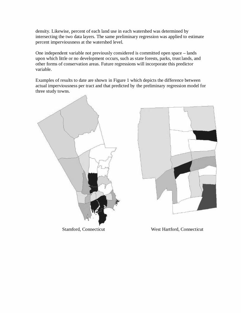
density. Likewise, percent of each land use in each watershed was determined by intersecting the two data layers. The same preliminary regression was applied to estimate percent imperviousness at the watershed level. One independent variable not previously considered is committed open space – lands upon which little or no development occurs, such as state forests, parks, trust lands, and other forms of conservation areas. Future regressions will incorporate this predictor variable. Examples of results to date are shown in Figure 1 which depicts the difference between actual imperviousness per tract and that predicted by the preliminary regression model for three study towns.

Stamford, Connecticut West Hartford, Connecticut

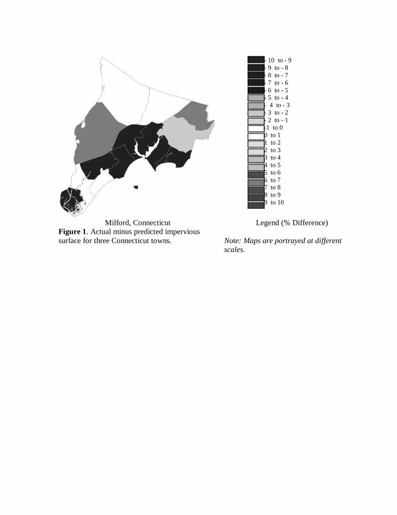
- 10 to - 9 - 9 to - 8 - 8 to - 7 - 7 to - 6 - 6 to - 5 - 5 to - 4 - 4 to - 3 - 3 to - 2 - 2 to - 1 -1 to 0 0 to 1 1 to 2 2 to 3 3 to 4 4 to 5 5 to 6 6 to 7 7 to 8 8 to 9 9 to 10

Milford, Connecticut Legend (% Difference) Figure 1. Actual minus predicted impervious surface for three Connecticut towns.

Note: Maps are portrayed at different scales.

Student Support Funds from this project have been used to support an MS-degree student, Anna Chabaeva, concentrating in earth resources information systems within the Department of Natural Resources Management and Engineering. Ms. Chabaeva has been the analyst largely responsible for data reformatting and analysis. Publications There have been no publications from this research as of yet. However, given the promising results thus far, it is expected that an abstract for a paper and presentation will be submitted for the ASPRS 2004 Annual Convention8. Also, there are plans for at least one peer-reviewed article. Ms. Chabaeva’s Master’s thesis will be yet another outlet for the results. And lastly, the results of this research will form the basis of a chapter of a manual on methodologies for impervious surface measurement. Information Transfer Once the impervious surface prediction model has been finalized, it will be applied to spatial data for the entire state of Connecticut and made available on the Internet by way of ArcGIS Server and ArcIMS. FGDC-compliant metadata9 will accompany the map data. These products will become part of a website on impervious surface and located on the NAUTILUS10 server (http://resac.uconn.edu).

Submitted 27 June 2003

8 American Society for Photogrammetry and Remote Sensing, http://www.asprs.org/denver2004call.pdf 9 Federal Geographic Data Committee, http://www.fgdc.gov/metadata/meta_stand.html 10 Northeast Applications of Usable Technology In Land planning for Urban Sprawl, a NASA Regional Earth Science Applications Center (RESAC).

ADDITIONAL REFERENCES:

Arnold, C.L and C.J. Gibbons. 1996. Impervious surface coverage: the emergence of a key environmental indicator. Journal of the American Planning Association 62(2), pp. 3243-258. Cappiella, Karen and Kenneth Brown. 2001. Imervious Cover and Land Use in the Chesapeake Bay Watershed. Center for Watershed Protection, Ellicott City, MD. 55 p. Civco, D.L. and J.D. Hurd. 1991. Multitemporal, multisource land cover mapping for the state of Connecticut. in Proc. of the 1991 Fall Meeting of the American Society for Photogrammetry and Remote Sensing, Atlanta, GA. pp. B141-B151. Civco, D.L., D.R. Miller, J.D. Hurd and Y. Wang. 1991. Connecticut statewide land use and land cover mapping. Project Completion Report for U.S. EPA-Conn. DEP Joint Long Island Sound Research Project CWF 219-R. 44p. Civco, D.L., C.L. Arnold and J.D. Hurd. 1998. Land use and land cover mapping for the Connecticut and New York portions of the Long Island Sound watershed. Project Completion Report for Conn. DEP Long Island Sound Research Fund CWF 330-R. Environmental Protection Agency. 1994. The Quality of Our Nation’s Water: 1992. United States Environmental Protection Agency #EPA-841-S-94-002. Washington, DC: USEPA Office of Water. Prisloe, M., Giannotti, L. and W. Sleavin. 2000. “Determining Impervious Surfaces for Watershed Modeling Applications.” Proceedings of the 8th National Nonpoint Source Monitoring Workshop.” Hartford, CT. Sept. 10-14. (in press) Prisloe, S., Y. Lei and J.D. Hurd. 2001.Interactive GIS-based Impervious Surface Model. Proc. 2001 ASPRS Annual Convention, St. Louis, MO. Schueler, T. R., 1994. The Importance of Imperviousness. Watershed Protection Techniques, vol. 1(3): pp. 100-11. Schueler, T. R. 2002. The Importance of Imperviousness Revisited. Center for Watershed Protection, Ellicott City, MD. (in press) Sleavin, W. J., 1999. Measuring Impervious Surface in Connecticut Using Planimetric GIS Data. Thesis, University of Connecticut, Storrs, CT. 126 p. Sleavin, W., S. Prisloe, L. Giannotti, J. Stocker, D.L. Civco. 2000. Measuring Impervious Surfaces for Non-point Source Pollution Modeling. Proc. 2000 ASPRS Annual Convention, Washington, D.C. 11 p.

Information Transfer ProgramThe CT IWR solicits proposals for information transfer projects as a part of its competitive RFP processdescribed above. In addition to these external projects, the institute conducts a number of activitiesthrough its technology transfer initiative project.

Water Resources Technology Transfer Initiative

Basic Information

Title: Water Resources Technology Transfer Initiative

Project Number: 2002CT5B

Start Date: 3/1/2002

End Date: 2/28/2004

Funding Source: 104B

Congressional District: 2nd

Research Category: Not Applicable

Focus Category: , Water Quantity, Water Supply

Descriptors:

Principal Investigators: Glenn Warner, Glenn Warner

Publication

1. Golf Course Water BMP Advisory Committee, 2001, "Report of the Advisory Committee OnPotential Best Management Practices For Golf Course Water", Connecticut Institute of WaterResources, University of Connecticut, Storrs, CT, 75pp.

Title: Water Resources Technology Transfer Initiative Principal Investigator(s): Glenn Warner and Patricia Bresnahan Congressional District: 2nd Problem Statement There are a number of academic researchers in Connecticut and within the New England re gion working on water resources problems. The information and techniques being developed by their research is of value and interest to state agencies, the private sector, and the general public. There are three levels of information exchange that need t o be addressed in order to ensure that the information gets to the people who need it:

• General awareness: members of the academic community need to be aware of the work that has been done or is in progress by researchers outside their immediate circle of peers. People outside of the academic community need to be aware of current and previous work, and to have access to that information. The CT IWR office maintains a small library of reports and publications generated from previous projects. Some, but not all, of this work is available through peer-reviewed publications. In some cases only one remaining paper copy of the original report exists. There is a need to both preserve this information and to disseminate it more widely.

• Focused attention on a specific issue: There is often a need to determine the state -of-the-art of knowledge on a specific water resource topic, especially as government agencies attempt to move towards science-based policy.

• Focused attention on a specific technique or technology: It is not financially feasible for every academic department dealing with water resources to maintain the staff and equipment necessary to train new professionals in all the latest techniques. As a result, each institution tends to develop one or two unique areas of expertise, limiting the exposure of students to new technology.

Summary of Information Transformation Program Seminar Series This year (2002-2003) the Institute sponsored six seminars with a general theme of "Beyond the Drought: A Closer Look at Water Supply and Demand in Connecticut." The theme and individual topics were selected based on needs that emerged during discussions that took place as a part of the Water Planning Council activities.

CT IWR 2002 - 2003 Seminar Series Wednesday, October 9, 2002

“Rainfall in Connecticut.”��� ����� ���� �� �� ������ �������� ��������� ��� ������������ ���������� �� �����������

Wednesday, November 13, 2002 “The Quinnipiac Watershed: Preliminary Assessment of Water Withdrawals

and Streamflows.”������ �������� ��� ����� �����!���� "����� �� #���� ���������� ����������� �� ������� ��

������������ ����������

Wednesday, December 11, 2002 “Water Supply Planning: Inter-basin and Inter-jurisdictional Issues.”

�� � ��� ������$�� ����������� ���� �� ������������ %&�� '����!� ��������

Wednesday, February 12, 2003 “Modeling of Water Resources in the Pawcatuck River Basin”(������ "���� )���������� �� � (������� ������ ������������ * ����� +���� ���������

Wednesday, March 12, 2003 “The Connecticut Drought Management Plan."

�� '!������� ������� �������� ����� ����� ���� ��� ������� ��������� ,����� �� ����� ��� ��������� Wednesday, April 9, 2003

“Public Water Systems: The Effect of Rates on Demand.”��� -��� )�.���� ���������� ������� ������ ��� ������������ ���������� �� � ������������ ����������

'������

Golf Course Compliance Assistance Project In November of 2000, the Connecticut Department of Environmental Protection (DEP) and the Connecticut Institute of Water Resources (IWR) began collaborating on water management information transfer project. The focus of the project was to facilitate the development of a list of potential Best Management Practices (BMPs) for Golf Course Water and to manage an outreach effort to include a one-day conference for industry professionals. The CT IWR received $30,000 for this effort. This project concluded in November, 2002. Publications

Rainfall Publication.

We have a manuscript in preparation, authored by Dave Miller and Glenn Warner, that will deal with historical precipitation patterns in Connecticut. This will be published as and IWR Special Report, and will be available both in .pdf format through our web site, and as a hard copy publication.

Digital Archives Project.

As part of the Water Resources Technology Transfer Initiative, CT IWR is collaborating with the UCONN Homer Babbage Library on a digital archive project. The library has agreed to donate $2500 towards this project. The library will be covering the expenses of having the IWR Special Reports series professionally scanned and saved in both .tif and searchable .pdf format. The library will also be updating their catalog database to make sure these are included. Eventually, the scanned articles themselves will be stored and accessible through the library's web server, through a web interface developed and maintained by the library. Mark Hood, a graduate student supported by IWR has been working closely with the library on this project, and has compiled a list of keywords for each article to be included in the "metadata" tables. The CANR liaison librarian, Jonathan Nabe, has been instrumental in obtaining library support for this project. Jonathan hopes that it can serve as a model for others of its type at both at UCONN and within the regional IWR system.

Student Support

Student Support

CategorySection 104Base Grant

Section 104RCGP Award

NIWR-USGS Internship

Supplemental Awards

Total

Undergraduate 2 0 0 0 2

Masters 8 0 0 0 8

Ph.D. 0 0 0 0 0

Post-Doc. 0 0 0 0 0

Total 10 0 0 0 10

Notable Awards and AchievementsThe CT IWR is administering the Fenton River Aquatic Study for the Univ. of CT, Department ofFacilities. The project began November 1, 2002 and is scheduled to end December 31, 2004. The purposeof the study is to determine the potential impacts of withdrawals from the UConn water supply wells thatlie in the floodplain of the Fenton river on the flow and fisheries habitat in the Fenton. There are threecomponents to the study: surface water flow in the Fenton and its tributaries, ground water levels atdifferent levels and positions and fisheries habitat and fish use of the Fenton. The study team consists ofFred Ogden (Civil and Environmental Engr.), George Hoag (Civil and Environmental Engr.), GlennWarner (Natural Resources Management and Engineering), Jeff Starn (USGS) and Piotr Parasiewcisz(Cornell) and Rick Jacobson (Natural Resources Management and Engineering). The interactions ofsurface-ground water will be measured and mathematically modeled at different water levels. Fish habitatand fish use will be monitored and used to develop a PHABSIM model. Total study cost is $ 571,089. ATechnical Advisory Group consisting of representatives from State and Federal agencies andenvironmental groups provides technical input to the study.

Publications from Prior ProjectsNone