Institut für Hydrologie - uni-freiburg.de · Institut für Hydrologie der...
147
Transcript of Institut für Hydrologie - uni-freiburg.de · Institut für Hydrologie der...


Institut für Hydrologie der Albert-Ludwigs-Universität Freiburg i.Br.
Matthias Retter*
Exploring subsurface flowpaths
at the Low Pass field site, Oregon, USA
Referent: Prof. Dr. Ch. Leibundgut
Koreferent: Dr. S. Uhlenbrook
Diplomarbeit unter der Leitung von Prof. Dr. Ch. Leibundgut
Freiburg i.Br., November 2003
-------------------------------------------------------- * corresponding address: [email protected]
Table of contents I
Table of contents
Preface ...................................................................................................1
1 Introduction.........................................................................................1
2 Literature review.................................................................................3
2.1 Runoff generation processes at hill slope scale............................................................3 2.2 Plot scale: Subsurface Flow processes ........................................................................4 2.4 Conclusions...................................................................................................................8
3 Site description...................................................................................9
3.1 General .........................................................................................................................9 3.2 Climate ........................................................................................................................10 3.3 Geology and geomorphology ......................................................................................11 3.4 Soils ............................................................................................................................12 3.5 Vegetation ...................................................................................................................15 3.6 Overview of the hillslope site.......................................................................................16 3.7 Conclusions.................................................................................................................16
4 Methods.............................................................................................17
4.1 Field methods..............................................................................................................17 4.1.1 Determination of precipitation...............................................................................19 4.1.2 Tipping buckets ....................................................................................................20 4.1.3 Electrical conductivity ...........................................................................................20 4.1.4 Automatic sampling setup ....................................................................................21 4.1.5 Bromide probe......................................................................................................21 4.1.6 Piezometer ...........................................................................................................22 4.1.7 Suction cup lysimeter ...........................................................................................23 4.1.8 Mini v-notch weir ..................................................................................................24 4.1.9 Soil moisture probes.............................................................................................25
4.2 Experimental hillslope table ........................................................................................26 4.2.1 Table itself ............................................................................................................26 4.2.2 Soil filling ..............................................................................................................27

Table of contents II
4.2.3 Rain simulator ......................................................................................................28 4.2.4 Tipping buckets at table .......................................................................................30 4.2.5 Mini-wells for water sampling ...............................................................................31 4.2.6 Piezometers at table.............................................................................................31 4.2.7 Soil moisture probes.............................................................................................32
4.3 General information on the applied tracer...................................................................33 4.4 Characteristics of the tracer experiments....................................................................36 4.5 Data analysis...............................................................................................................38 4.6 Conclusions.................................................................................................................41
5 Results and discussion: Field investigations................................42
5.1 Description of soil pipes ..............................................................................................42 5.2 Precipitation ................................................................................................................43 5.3 Soil pipe flow ...............................................................................................................47
5.3.1 Timing of soil pipe flow and flux ...........................................................................49 5.3.2 Discussion of soil pipe flow ..................................................................................50
5.4 Dynamic contributing area of soil pipes ......................................................................51 5.5 Piezometer results ......................................................................................................52
5.5.1 Water table levels.................................................................................................52 5.5.2 Timing of water table establishment.....................................................................55 5.5.3 Spatial presentation of water table .......................................................................56 5.5.4 Discussion of water table and flow mechanisms..................................................59
5.6 Discharge at weir ........................................................................................................61 5.7 Results tracer experiments .........................................................................................63
5.7.1 Amio G Acid .........................................................................................................63 5.7.2 Bromide application..............................................................................................65 5.7.3 Discussion of tracer results ..................................................................................67
5.8 Conclusions of field investigations ..............................................................................68
6 Results and discussion: Hillslope table.........................................71
6.1 Short overall description of the experimental run........................................................71 6.2 Sprinkling ....................................................................................................................71 6.3 Runoff..........................................................................................................................72 6.4 Water balance .............................................................................................................74 6.5 Soil moisture ...............................................................................................................74 6.6 Water table and water volume ....................................................................................75 6.7 Tracer..........................................................................................................................80

Table of contents III
6.7.1 Amino G Acid line source .....................................................................................80 6.7.2 Discussion of Amino G Acid line source...............................................................83 6.7.3 Bromide................................................................................................................83 6.7.4 Discussion of bromide..........................................................................................84 6.7.5 Dye tracing with Brilliant Blue...............................................................................85 6.7.6 Discussion of dye tracing with Brilliant Blue .........................................................87
6.8 Conclusions of hillslope table......................................................................................87 6.9 Prospects for further experiments ...............................................................................87
7 Concluding remarks and outlook ...................................................88
8 References ........................................................................................90
Appendix A
Appendix B
Appendix C

Table of contents IV
List of figures Fig. 2.2: Hydraulic conductivity versus pressure head for sand and sandy loam; hydraulic
conductivity versus water content; relative hydraulic conductivity versus pressure head; and relative hydraulic conductivity versus saturation. 5
Fig. 2.2.1: Hydrological processes at infiltration. 7 Fig. 2.2.2: Macropores and live-root (white) in the soil behind a trench face in a forest floor. 7 Fig. 2.3: Conceptual model of runoff generation at the Maimai hillslope, New Zealand. 8 Fig. 3.1: Location of field site and near climate stations. 9 Fig. 3.2: Monthly climate summary for Noti. 11 Fig. 3.4a: Soil characterisation. Beside forest road is the trench excavation with visible soil face
(cutslope) of hillslope investigated. 13 Fig. 3.4b: Cutslope along the forest road about 200 m further away of the hillslope. 13 Fig. 3.4c: Soil profile of P_B4 up to a depth of 120 cm. 14 Fig. 3.4d: View of trench below hillslope with location of the three soil pipes. 15 Fig. 4.1a: Overview of instrumentation around data logging unit at Low Pass field side. 17 Fig. 4.1b: Overview on investigated hillslope with instrumentation and extended catchment of a
first order stream. 18 Fig. 4.1.1: Throughfall gauging below canopy layer of mixed forest. 20 Fig. 4.1.8: Flume with WT-HR water height recorder. 25 Fig. 4.2.1: Artificial hillslope table and rainfall simulator. 27 Fig. 4.2.3a: Shape of table, dividing for collection chambers of tipping buckets piezometers, soil
moisture sensors and location of sampling wells. 29 Fig. 4.2.3b: Distribution of sprinkling intensities (mm/hr) along different transects of table. 30 Fig. 4.2.6: Three water table loggers at the side of the experimental table. 32 Fig. 4.3.1a: Structure of Amino G Acid. 34 Fig. 4.3.1b: Adsorption of Amino G Acid on humus sediment. 35 Fig. 5.2a: Open land precipitation at the climate station Eugene, for overall investigation period
and long-term mean. 44 Fig. 5.2b: Daily rainfall at field site Low Pass and pipe flow for study period. 45 Fig. 5.2c: Rainfall intensities per 10 min for selected interval, additionally hydrograph. 45 Fig. 5.3a: Pipe flow shown in logarithmic scale and branches used for recession analysis. 47

Table of contents V
Fig. 5.3b: Recession of mean discharge over recession branch and mean turnover time for selected events. 49
Fig. 5.5.1a: Water table at various piezometers, pipe flow and throughfall. 53 Fig. 5.5.1b: Water table levels at piezometers in row A ahead, while and after ID 4. 54 Fig. 5.5.1c: Water table levels at piezometers in row C ahead, while and after ID 4. 54 Fig. 5.5.3: Spatial distribution of water table at lower part of hillslope ahead, while
and after ID 4. 57-58 Fig. 5.6a: Discharge of weir, soil pipes, and standardized weir flow. 61 Fig. 5.6b: Time shift of pipe flow and weir hydrograph for event related to tracer injection. 62 Fig. 5.7.1: Concentration of Amino G Acid at suction lysimeter below the line source tracer
application. 64 Fig. 5.7.2a: Electrical conductivity after the tracer application, discharge soil pipes and precipitation. 65 Fig. 5.7.2b: Bromide concentration at bottom suction lysimeter. 66 Fig. 5.8: Assumed processes and conditions along transect of the hillslope. 69 Fig. 6.2: Overview on sprinkling and runoff for the whole experiment at the hillslope table. 72 Fig. 6.3: Variability of accumulated discharge at different tipping buckets and sprinkling intervals. 73 Fig. 6.5: Soil moisture at three different locations at the table for the period of experiment. 74 Fig. 6.6a: Height of water table at different time steps. 76-78 Fig. 6.6b: Sprinkling, runoff and water volume for the first interval of the experiments. 79 Fig. 6.7.1a: Amino G concentration and discharge at TB 8. 81 Fig. 6.7.1b: Amino G concentration, accumulated discharge and sprinkling for TB 8. 82 Fig. 6.7.1c: Accumulated discharge and Amino G concentration at TB 8. 82 Fig. 6.7.3a: Bromide concentrations, electrical conductivity, sprinkling intervals and accumulated
discharge at TB 1. 84 Fig. 6.7.5a: Line source of Magic blue at y=290 cm and dye movement down slope. 86 Fig. 6.7.5b: Documentation of Brilliant Blue pathways at y=265 cm. 86 Fig. 6.7.5c: Documentation of Brilliant Blue pathways directly at the line application (y= 290 cm). 86

Table of contents VI
List of tables Tab. 3.2: Documentation of climate stations and amount of total annual precipitation. 10 Tab. 4.3.1: Amino G Acid adsorption on mineral and organic materials. 34 Tab. 5.1: Features of soil pipes. 42 Tab. 5.2: Selected characteristic of rainfall and runoff attributes for the hillslope and pipeflow. 46 Tab. 5.3: Recession analysis of selected events and storage coefficient of the system. 48 Tab. 5.4: Pipe flow records, DCA and runoff coefficients. 51 Tab. 5.5.2: Data of selected piezometer on selected events, including time shift. 55

Table of contents VII
List of figures in appendix Fig. A2a: Sabre growth indicating the soil creeping at the Low Pass field site. Fig. A2b: Sabre growth indicating the soil creeping. Fig. A3: Discharge soil pipes and rain events for the period of hydrograph separation. Fig. A4: Slug test at P_D3 on March, 25 2003. Fig. A5: Water table at P_A3 and runoff soil pipes. Fig. A6: Correlation between water table and pipe flow for selected piezometers. Fig. B1: Amino G breakthrough, accumulated discharge and sprinkling intervals at TB 1. Fig. B2: Amino G breakthrough, accumulated discharge and sprinkling intervals at TB 2. Fig. B3: Amino G breakthrough, accumulated discharge and sprinkling intervals at TB 3. Fig. B4: Amino G breakthrough, accumulated discharge and sprinkling intervals at TB 4. Fig. B5: Amino G breakthrough, accumulated discharge and sprinkling intervals at TB 5. Fig. B6: Amino G breakthrough, accumulated discharge and sprinkling intervals at TB 6. Fig. B7: Amino G breakthrough, accumulated discharge and sprinkling intervals at TB 7. Fig. B8: Correlation between electrical conductivity and bromide concentration of flow proportional hand samples at TB 1. Fig. B9: Correlation between electrical conductivity and bromide concentration of flow proportional hand samples at TB 1, for the times < 19.5. Fig. B10: Correlation between electrical conductivity and bromide concentration of flow proportional hand samples at TB 8. Fig. B11: Bromide concentrations, electrical conductivity, sprinkling intervals and accumulated
discharge at TB 8. Fig. C1: Sketch of tipping buckets to provide a visual impression for information purposes. Fig. C2a: Water height recorder WT-HR. Fig. C2b: Sketch of PVC-pipe which encased the water table recorder, to be placed in a drill hole. Fig. C3a: Construction plan for triangular-notch weir. Fig. C3b: Details of notch. Fig. C3c: Rating curve of “v”-notched weir. Fig. C4: Sketch of soil water sampler. Fig. C5: Sketch and circuit diagram of electrical conductivity probe.
Fig. C6: Structure of a mini-well for water sampling.

Table of contents VIII
List of tables in appendix Tab. A1.1: Field sheets, soil profile at P_A1. Tab. A1.2: Field sheets, soil profile at P_A3. Tab. A1.3: Field sheets, soil profile at P_A5. Tab. A1.4: Field sheets, soil profile at P_A7. Tab. A1.5: Field sheets, soil profile at P_A9. Tab. A1.6: Field sheets, soil profile at P_B1. Tab. A1.7: Field sheets, soil profile at P_B2. Tab. A1.8: Field sheets, soil profile at P_B4. Tab. A1.9: Field sheets, soil profile at P_C1. Tab. A1.10: Field sheets, soil profile at P_C3. Tab. A1.11: Field sheets, soil profile at P_C5. Tab. A1.12: Field sheets, soil profile at P_C7. Tab. A1.13: Field sheets, soil profile at P_C9. Tab. A1.14: Field sheets, soil profile at P_D1. Tab. A1.15: Field sheets, soil profile at P_D3. Tab. A1.16: Field sheets, soil profile at P_D5. Tab. A3: Exact data on hydrograph separation for selected runoff events. Tab. A4: Determination of input mass for Low Pass experiment. Tab. A5: Calculation on assumed drainage geometry of soil pipes. Tab. B1: Information on irrigation intervals during experiments at hillslope table.

Table of contents IX
Abbreviations and synonyms API7 - Antecedent 7-days precipitation index [mm] DCA - Dynamic contributing area [m²] DOC - Dissolved organic carbon
EC - Electrical conductivity [µS/cm] ID - Assigned identification number for runoff peaks L_B - Bottom lysimeter L_U - Upper lysimeter P_[row][number] - Piezometer,
includes alpha-numerical identification code Q - Discharge, runoff [l/10 min] R² - Coefficient of determination [-] r ² - Correlation coefficient [-] TB - Tipping buckets W - Weir, flume Ψ - Runoff coefficient [-]

Table of contents X
Summary
Intense field studies and tracer studies illuminate the characteristics of subsurface flow at an
unchanneled hillslope in the Oregon Coast Range, USA. The investigations presented, are
based on the period March - May 2003. The soil order of the site is classified as an
Inceptisols, series Bohannon sandy loam. The focus of investigation were three soil pipes
(diameter up to 12 mm), which occurred at a soil depth of 1.8 m. An excavated trench at the
bottom of the hillslope provided the opportunity to study pipe flow and interflow out of the
hillslope. Supplementary, the initial first order stream at the convergence of hillslope, 50 m
below the trench, was kept under surveillance.
Outflow of the hillslope was restricted to the pipes and no other interflow occurred. While the
face of the cutslope in the south showed high moisture content, no major water table
oscillation was found behind in the hillslope. Contrary, in the north part, with less hillslope
convergence, trench faces remained completely dry and water tables behind showed
significant changes, with a magnitude up to 60 cm below surface topography. Further,
temporal data of water tables in the hillslope yielded information to identify its quick response
to rainfall events. Peaks of water tables occurred about 11 hr before pipeflow peaks,
although there was some variation due to individual piezometer response.
Pipe flow (sum of the three pipes) responded quickly to rainfall input during the first months.
Observations that pipe flow became more important when rainfall intensities were
extraordinary high could not be confirmed in this study. A recession analyses of the
hydrograph showed the pattern of quick turnover times for high mean discharge conditions.
Later in the year, when soil moisture was strongly diverse from field capacity, no response
was observed. Pipe flow ran dry in June, effected by the seasonal rainfall characteristics in
Western Central Oregon.
The calculation of the dynamic contributing area of the soil pipes (DCA) helped to classify the
soil pipes. The result (max DCA) amounted to at least 9500 m², although there is some
uncertainty included. A further attempt on the characterisation of the soil pipe’s drainage
network is presented by a land drainage approach based on the HOOGHOUDT-equation. A
rough estimation on the distance between draining pipes (original idea of parallel pipes)
varied around 1 m. Further, data of the weir below the trench, are presented with a
hydrograph time shift of 7 hr compared to the pipe flow peak.
An Amino G Acid line injection into the upper soil did not reveal any tracer breakthrough at
the soil pipes as well as at the initial first order stream. Bromide sprayed over a wide range of
the hillslope was not detected in pipe flow, either. Observations of suction cup lysimeter
(depth 30, 50 and 70 cm) showed both tracers remaining in the unsaturated zone. Thus, dye

Table of contents XI
residence times in the unsaturated zone are controlled by quantity of injected tracer and
amount of rainfall.
To extent the possibilities of investigation, an experimental model of the hillslope – an
artificial hillslope table – was used in a parallel approach. This physical modelling allowed the
same tracer experiments as in the field under triggered conditions. Sprinkling intervals were
adjusted to rainfall characteristics of the Oregon Coast Range. Bromide added to the
sprinkler water moved through the soil as plug flow controlled by rainfall rate and water
content. The Amino G Acid line source experiments at the table verified that unsaturated
conditions limit tracer movement in the upper part of the slope. A final excavation of Brilliant
Blue, although an adsorptive tracer, corroborated the restricted movement in the sandy loam.
Moreover, this suggests the high influence of soil pipe structures in this soil. By these
findings the outlook of this work does encourage a next generation of physical modelling at
the table with implemented artificial soil pipe structures in the soil. This would help to address
the question of how runoff concentration and response time change in case of soil pipes
acting.
Keywords: Oregon Coast Range, field study, preferential pathway, soil pipe, trench based investigation, physical model, sprinkling experiments

Table of contents XII
Zusammenfassung
Zielsetzung der Arbeit war es, Kenngrössen und Prozesse von underirdischen Fließwegen in
einem gerinnelosen Hang der Oregon Coast Range, USA, zu untersuchen, wozu eine
Feldkampagne mit Datenerhebung und Markierversuche durchgeführt wurden. Die
vorliegenden Resultate stammen hauptsächlich aus dem Untersuchungszeitraum März bis
Mai 2003. Eine Bodenklassifizierung am Untersuchngshang wies einen sandigen Lehm der
Bahannon Serie aus. Kern der Untersuchung waren drei erweiterte Makroporen, im
folgenden als soil pipes bezeichnet, die in einer Bodentiefe von 1,8 m auftraten und
Durchmesser bis 12 mm aufwiesen. Mit Hilfe eines quer angelegten Untersuchungsgrabens
am unteren Ende des Hangs konnte das Abflußverhalten der soil pipes und der
Zwischenabfluss aus der Hangfläche untersucht werden. Zusätzlich wurde der 50 Meter
unterhalb des Grabens auftretende Gewässerlauf erster Ordnung zur Analyse
herangezogen.
Ausfluß aus der Hangfläche fand lediglich über die soil pipes statt, da kein Zwischenabfluß
im Querschnitt auftrat. Die Abbruchkante des Grabens zum Hang hin zeigte in der südlichen
Hälfte hohe Oberflächenfeuchtigkeit, doch traten Wasserspiegel im Hang selbst nur restriktiv
auf. Dem gegenüber stehend, fanden sich in der nördlichen Hälfte, die jedoch weniger
topographische Konvergenz zeigt, permanent ausgetrocknete Oberflächen und ein
bedeutender Wasserspiegel mit Schwankungen bis 60 cm unter Geländeoberkante.
Weiterhin ergab die zeitliche Auswertung der Wasserstandsdaten wichige Informationen zur
Erkennung der schnellen Systemantwort auf Niederschlagsereignisse. Obwohl die Daten der
individuellen Piezometern eine hohe Variation zeigte, zeigte sich ein Nacheilen des soil pipe
-Spitzenabflusses um 11 Stunden zu den Spitzen des Wasserstandes im Hang.
Der Abfluß aus den soil pipes (Aufsummierung der drei einzelnen soil pipes) zeigte eine
schnelle Antwort auf Niederschlag während den ersten Monaten. Beobachtungen, dass soil
pipe-Abfluß bei hohen Niederschlagsintensitäten eine dominantere Ausprägung erfährt,
konnten durch diese Studie nicht belegt werden. Eine Rezessionsanalyse der Ganglinien
zeigte den Zusammenhang von schnellen turnover times bei hohen mittleren Abflüssen. Zu
späteren Zeitpunkten, bei einer Bodenfeuchte, die von der Feldkapazität weit entfernt lag,
konnte keine Abflussreaktion aus Niederschlagsereignisse festgestellt werden. Das
Versiegen der soil pipes im Juni ist durch das starke Saisonalität des Niederschlags mit
verbundener Trockenheit im zentralen, westlichen Oregon zu begründen.
Um die soil pipes genauer beschreiben zu können, half die Berechnung einer dynamischen
Beitragsfläche (dynamic contributing area, DCA), also einer Art Einzugsgebiet der soil pipes.
Eine Fläche (max. DCA) von mindestens 9500 m² wurde abgeschätzt und die Unsicherheiten
diskutiert. Ein weitere Ansatz zur Charakterisierung des Einzugsgebeites der soil pipes

Table of contents XIII
erfolgt mit einem Drainierungsansatz der Entwässerungstechnik, welcher auf der Formel von
HOOGHOUDT basiert. Eine grobe Abschätzung zu dem Abstand zwischen einzelnen soil pipes
(ursprüngliche Idee von parallelen Rohren) variiert um 1 m für verschiedene Ereignisse und
Annahmeparameter. Weiterhin ergab sich für den Abfluß am Gerinne erster Ordnung
(Überfallwehr), verglichen mit dem Spitzenabfluss der soil pipes, eine Zeitverschiebung in
der Ganglinie von 7 Stunden.
Ein Markierversuch (Injektion einer Linie aus Amino G Acid) in 5 cm Bodentiefe ergab keinen
Markierstoffnachweis am Auslass der soil pipes sowie auch nicht am Überfallwehr. Ein
weiterer flächenhafter Eintrag vom Lithiumbromid auf den Hang konnte ebenfalls nicht im
Abfluß der soil pipes nachgewiesen werden. Die aus Saugkerzen entnommenen Proben in
Tiefen von 30, 50 and 70 cm zeigten ein Verbleib des Markierstoffes in der ungesättigten
Zone. Die Aufenthaltszeiten und die Mobilisierung von Markierstoff ist somit abhängig von
der Einspeisemenge und von der gefallenen Niederschlagsmenge.
Um in einem weiteren Schritt die Untersuchungsmöglichkeiten zur Bedeutung von
unterirdischen Fliesswegen zu erweitern, wurde ein experimentelles Modell des
Untersuchungshanges – ein künstlicher Hangtisch – in die Studie integriert. Diese
physikalische Modellierung erlaubte ähnliche hydrometrische Erfassung und die gleichen
Markierversuche wie im Feld unter steuerbaren Bedingungen. Die künstlichen
Beregungsintervalle wurden dabei abgestimmt auf die Characteristika der Küstenkette von
Oregon.
Das mit Bromide versetzte Beregungswasser bewegte sich durch den Boden in einer Front,
welche durch Beregungsintervalle und Bodenwassergehalt maßgeblich gesteuert wurde. Die
Ergebnisse des linienhaften Markierexperiments mit Amino G Acid bestätigten, dass die
ungesättigten Bedingungen den Stofftransport im oberen Teil des Hanges begrenzen. Die
schlussendliche Ausgrabung eines weiteren, jedoch absorbierenden Markierstoffes, Brilliant
Blue, erhärtete die Erkenntniss von eingeschränkter Fortbewegung im sandigen Lehm.
Ferner verdeutlichte dies die tatsächliche Bedeutung von soil pipe Stukturen in diesem
Boden. Basierend auf diesen Erkenntnissen ermutigt der Ausblick dieser Arbeit eine nächste
Generation von physikalischen Modellen am Hangtisch mit künstlich eingebauten soil pipe
Strukturen. Dies wäre hilfreich für die Fragestellung inwieweit Abflußkonzentration und
Systemantwort sich unter den Bedingungen von fungierenden soil pipes verändern.

Preface, Introduction 1
Preface This research was conducted at the Watershed Laboratory of the Dept. of Forest
Engineering, Oregon State University, USA and the Institute of Hydrology, University of
Freiburg, Germany. It was supported by the Förderverein Hydrologie and financial
assistance was recieved through “Eliteförderprogramm der Landesstiftung Baden-
Württemberg GmbH” (research grant: “Einsatz geophysikalischer Methoden in Verbindung
mit Tracermethoden in der Abflussbildungsforschung"). The project also received
comprehensive support from the chair of Prof. Dr. J. McDonnell.
1 Introduction In one of the earliest investigations of runoff generation, HURSH (1936) detected that
subsurface flow, and not overland flow, was the source of storm runoff in forested
catchments. Since then the mechanisms of subsurface flow paths have been the focus of
much discussion and debate. Studies have shown that so called preferential pathways play
an important role in runoff generation of forested hillslopes (e.g. BEVEN & GERMANN, 1982;
BRONSTERT, 1999; MCGLYNN et al., 2002). The term preferential pathways includes
macropores and other open structures, where water can move through the soil rapidly.
Macropores occur in various soil types and are frequently found in slopes, often in a well
connected network. Larger macropores are commonly referred as ‘soil pipes’ (e.g. JONES,
1971). Numerous hydrologists have performed tracer experiments to gain knowledge on the
subsurface flow processes (MCDONNELL et al., 1998; SKLASH et al., 1996). Tracer
information at the catchment outlet is treated as convergent or integrated data respectively
as integration of individual hillslope processes (LEIBUNDGUT, 1984). Results have shown the
high velocity of pipe flow (MOSLEY, 1982) and its relationship to soil water content and
groundwater levels (MCDONNELL, 1990; CROZIER et al., 2003). UCHIDA et al. (1999) have
noted the lack of discharge rates of pipe flow and stream flow in mountainous watersheds.
Despite many years of study, subsurface flow pathways are still poorly understood. It may
occur in highly permeable soil layers overlying low permeable layers, or in preferential flow
pathways and more permeable (weathered) areas in the soil or at the soil bedrock interface.
Introduction 2 Studies have shown that often “threshold mechanisms” of either rainfall intensities or
antecedent moisture conditions (flow levels prior to storms) may trigger subsurface flow
(UCHIDA et al., 1999; JONES, 1997; MCDONNELL, 1990; ZIEMER & ALBRIGHT, 1987; JONES &
CRANE, 1984; WILSON & SMART, 1984). Nevertheless, the conversion of flow from vertical
pathways in the soil into lateral matrix or preferential flow pathways is poorly understood. In
general, the development of reliable methods to quantify the continuity and hydraulic
conductivity of macropores in situ for a range of field moisture conditions, at a scale and
depth sufficiently large to be useful for applying predictive models, is one of the greatest
challenges for researchers in vadose zone hydrology (STEPHENS, 1996).
Problem and Objective This diploma thesis examines preferential flow processes, and explores the connection of
vertical and lateral flow pathways at the hillslope scale. The study includes two main
approaches focusing on this detection of flow mechanisms: (1) investigation of a natural
forested hillslope in Western Oregon, USA, and (2) investigation of an artificial hillslope,
filled with material from the Oregon field site. Questions posed for both study components
included: How do soil pipes control hillslope response to storm rainfall? How does
topographic convergence affect subsurface flow? How do matrix and pipe flows couple at
the plot and hillslope scale?
To explore these topics, an intensive field campaign was conducted with various installed
hydrometric measurements. Subsurface flow volumes, flow timing rates, water table levels
and soil moisture conditions were determined over a period of March - May 2003. Further,
tracer experiments were performed during selected rainfall events and tracer transport
through the system with associated pipeflow was investigated. The physical hillslope
extended the field work with controlled rainfall experiments where runs were performed for
soils without and later with soil pipes. These experiments helped address the question of
how does runoff concentration and response time change, when artificially implemented soil
pipes are included in to matrix material (guided by the philosophy that hydrological science
is in greater need of more and better experimentation HORNBERGER & BOYER, 1995).
The final objective strives for the combination of knowledge gained by both approaches.

Literatur review 3
2 Literature review
A short outline on the important runoff generation processes related to the hill slope scale is
presented in the following. Thereafter a principle overview includes the hydrological
processes at the plot scale, where the focus highlights the characteristics of macropores.
2.1 Runoff generation processes at hillslope scale
Within recent decades, understanding of the processes in rainfall-runoff systems has
significantly improved. The classical dynamic-oriented division into surface flow, interflow,
and base flow can not keep up with the complexity of hill slope processes, which are being
described more and more precisely (GUTKNECHT, 1996). Nevertheless, a hill slope’s
response to rainfall will still be an interweaving of different components. Controlling factors
like rainfall characteristic, topography and antecedent soil moisture conditions regulate the
interaction of single processes in runoff generation.
Hortonian Overland Flow Component is overland flow that results from impermeable surfaces. The saturation from
above occurs where water-input rate exceeds the saturated hydraulic conductivity of the
surface layer. The process is not postulated for entire hill slopes, it rather fits to the partial-
area concept (DINGMAN, 2002; UHLENBROOK & LEIBUNDGUT, 1997).
Saturation Overland Flow Overland flow occurs as the result of saturation from below. Saturation Overland Flow is
performed by direct water input to the saturated area as well as by the return flow. This is of
importance near streams, where the water table is already close to the surface. Further, it
occurs at hill slope hollows (concavities), at concave slope breaks, where thin soil layers
conduct subsurface flow, and at perched conditions. This mechanism is linked to the
variable source area concept (DINGMAN, 2002; UHLENBROOK & LEIBUNDGUT, 1997).
Subsurface Flow Subsurface flow mechanisms describe the non visible transmission or movement of water
within the soil. Subsurface flow processes in soil may be separated in two domains: The
homogeneous matrix flow, and the flow through structural pores, referred to as preferential
flow. In the latter, water is primarily driven by gravity and is less obstructed by capillary
forces. In the domain of matrix flow, water is subjected to capillarity, where potential flow
approaches apply. The soil matrix here is quite often not completely saturated with water,
because the time required for its complete saturation may exceed the time needed to

Literatur review 4 establish flow in macropores (ANDERSON & BURT, 1990). Section 2.2 provides a more
detailed exposition on that topic. Second, processes may also be classified in temporal
categories. E.g. infiltrated event water is by this means able to mobilize stored pre-event
water in the near-stream zone. In particular because of its strong contribution to flood
events, subsurface flow has been investigated well (e.g. BERGMANN et al., 1996).
2.2 Plot scale: Subsurface Flow processes
Flow processes through field soils are in most cases highly irregular. There are vertical flow,
lateral flow, and solute transport all occurring. However, often these processes are mixed
up. For a start we focus on the vertically dominated processes.
a.) Matrix Flow Flow through the soil matrix is induced by, among other things, gravity and capillary forces in
the little micropores. These are defined as having an average diameter or thickness
smaller than 1/16 mm (CHOQUETTE & PRAY, 1970). Here, flow can occur in either saturated
or unsaturated conditions. The speed of flow depends on the hydrological conductivity of the
soil matrix, which itself is a function of the soil texture and the soil water content (BEVEN &
GERMANN, 1982). The dependence of hydraulic conductivity on water content is shown in
Fig. 2.2. Especially in the vadose zone, where a range of water contents is likely to be
encountered, the hydraulic conductivity has great variability.

Literatur review 5
Fig. 2.2: Hydraulic conductivity versus hydraulic conductivity versus w versus pressure head (C); and saturation (D). Corresponding capacity for these soils are no
b.) Preferential Flow This includes all processes where infil
soil (ANDERSON & BURT, 1990; LUXMO
often achieved. Factors affecting prefer
properties and profiles; and (3) rainfall
used as an umbrella term for the follow
Finger Flow Fingered flow occurs in a perfect hom
becomes unstable, breaks up like a flam
& NICHOL, 1996). Fingers may occupy o
the porous medium, an observation w
recharge of groundwater can occur lon
to point out that there has been more e
the importance of unstable flow.
Sandy clay loam Sand
pressure head for sand and sandy loam (A); ater content (B); relative hydraulic conductivity relative hydraulic conductivity versus percent
water retention curves and specific moisture t shown. From: STEPHENS (1996).
trating water is able to move better through the bulk
ORE, 1981). Here, by-passing is not necessary but
ential flow include: (1) soil structure; (2) soil hydraulic
intensity (MCINTOSH et al., 1999). Preferential flow is
ing presented:
ogeneous, sandy, porous medium. The wetting front
e front and splits into “fingers” (HILLEL, 1987; GLASS
nly a portion of the horizontal cross sectional area of
hich led THOMAS & PHILLIPS (1979) to conclude that
g before the soil is thoroughly wetted. It is important
xperimental laboratory work than field work to verify

Literatur review 6 Funnel Flow Funnel flow occurs when the downward water flow gets funneled or diverted towards one
side because of the barrier concept. For further details on this very special process see
WALTER et al. (2000).
Macropore Flow Out of the presented types of preferential flow, macropore flow is predominant and very
common. Macropores are structural pore spaces in the soil with a diameter of 3 to 100 mm
according to DINGMAN (2002), although other authors set the lower boundary higher
(overview in: LUXMOORE et al., 1990). Another definition is presented by LUXMOORE (1981)
for soil pores with matric potentials greater than -0.3 KPa and corresponding diameters
greater than one millimetre. BEVEN & GERMANN (1982) point out that size is not an absolute
criterion as long the structure of the pore allows episodic, turbulent flow. A review of different
definitions of macropores is provided by LUXMOORE (1981) and CHEN & WAGNER (1992).
The origins of macropores are root holes, earthworm channels, and other kinds of
biotubation like vole tunnels as well as shrinking cracks or fissures (BEVEN & GERMANN,
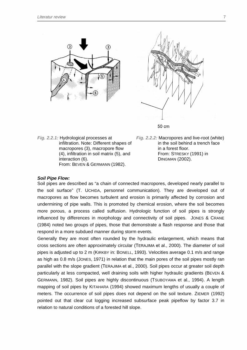
1982). The resulting types of macropores therefore differ (Fig. 2.2.1) and often establish a
wide, continuous, and diverse network (WANG et al., 1994). Fig. 2.2.2 gives an idea of the
interconnecting, three dimensional network. Water conductivity is more strongly related to
the continuity of a network than to pore size and shape (BOUMA et al., 1977).
Generally water can flow into macropores from the soil surface, or from the saturated or
partially saturated soil layer. Flow initiation is controlled by initial water content, rainfall
intensity, rainfall amount, hydraulic conductivity and surface contributing area (STEPHENS,
1996; PHILIP, 1993).
MOSLEY (1979) first found ample evidence that macropores can conduct water in
considerable distances through otherwise unsaturated soils at velocities of several
millimetres per second. Macropores allow the water to bypass the soil matrix, which is why
the term “bypass flow” is commonly used (ONODERA & KOBAYASHI, 1995). This is possible
under two main circumstances: Macropore flow with little or no interaction, and macropore
flow with high interaction with the surrounding soil matrix (MCLAREN & CAMERON, 1994).
Here, the potential gradient causing the macropore bypass flow, is not in equilibrium with the
gradient in the soil matrix. The water transfer between macropores and the surrounding soil
matrix depends on the properties of the surfacine of the macropore (BEVEN & GERMANN,
1982). There is also a general relation between the minimum pore diameter that will cause
bypassing and the pore size of the soil matrix (DINGMAN, 2002).
Literatur review 7
Fig. 2.2.1: Hydrological processes at infiltration. Note: Different shapes of macropores (3), macropore flow (4), infiltration in soil matrix (5), and interaction (6). From: BEVEN & GERMANN (1982).
Fig. 2.2.2: Macropores and live-root (white) in the soil behind a trench face in a forest floor. From: STRESKY (1991) in DINGMAN (2002).
Soil Pipe Flow: Soil pipes are described as “a chain of connected macropores, developed nearly parallel to
the soil surface” (T. UCHIDA, personnel communication). They are developed out of
macropores as flow becomes turbulent and erosion is primarily affected by corrosion and
undermining of pipe walls. This is promoted by chemical erosion, where the soil becomes
more porous, a process called suffusion. Hydrologic function of soil pipes is strongly
influenced by differences in morphology and connectivity of soil pipes. JONES & CRANE
(1984) noted two groups of pipes, those that demonstrate a flash response and those that
respond in a more subdued manner during storm events.
Generally they are most often rounded by the hydraulic enlargement, which means that
cross sections are often approximately circular (TERAJIMA et al., 2000). The diameter of soil
pipes is adjusted up to 2 m (KIRKBY in: BONELL, 1993). Velocities average 0.1 m/s and range
as high as 0.8 m/s (JONES, 1971) in relation that the main pores of the soil pipes mostly ran
parallel with the slope gradient (TERAJIMA et al., 2000). Soil pipes occur at greater soil depth
particularly at less compacted, well draining soils with higher hydraulic gradients (BEVEN &
GERMANN, 1982). Soil pipes are highly discontinuous (TSUBOYAMA et al., 1994). A length
mapping of soil pipes by KITAHARA (1994) showed maximum lengths of usually a couple of
meters. The occurrence of soil pipes does not depend on the soil texture. ZIEMER (1992)
pointed out that clear cut logging increased subsurface peak pipeflow by factor 3.7 in
relation to natural conditions of a forested hill slope.

Literatur review 8 2.3 Conclusions
The alignment of macropores does provide flow possibilities in vertical and also transverse
directions. Major characteristics are the rapid bypass of the soil matrix and the extended
network of macropores, which is able to drain a great area.
An overall summary of already detected mechanisms at a singled out, well studied hillslope
is shown in Fig. 2.3. The literature review shows that to date, not much is known about the
connection of lateral and transverse flow paths. Many studies show these mechanisms only
roughly and without details (e.g. Fig. 2.3).
Fig. 2.3: Conceptual model of runoff generation at the Maimai hillslope, New Zealand. From: MCDONNELL (1990).

Site description 9
3 Site description
3.1 General
The fieldwork was carried out at a forested hillslope in the Coast Range, Western Central
Oregon, United States of America. This site is called Low Pass with reference to its nearest
geographically important feature and is situated approximately 34 km west of Eugene
(Fig. 3.1). The United States Department’s Interior Bureau of Land Management is in charge
of the site and contracts Oregon State University, Corvallis, Oregon and the USDA Rocky
Mountain Research Station, Boise, Idaho for the research project. The hydrological
experimental setup in this catchment was established in autumn 2002 and in spring 2003.
This new phase of research is related to an earlier study, although with a different focus,
undertaken by the U.S. Forest Service. The features of this intensively studied single
hillslope are described later in Fig. 4.1b.
Fig. 3.1: Location of field site (indicated by star) and near climate stations.

Site description 10
3.2 Climate
The climate pattern of Central Oregon is dominated by the marine environment of the Pacific
Ocean associated with fronts and large moisture supply. Air containing moisture must rise to
pass over the mountain ranges and the vast majority of the precipitation falls on the western
side of the mountains, leaving the eastern side much drier. Therefore two major precipitation
gradients occur inland; first, at the Coastal Range and second, at the Cascades. In between
the two ranges is the interior, drier region Willamette Valley.
The study side is located east of the Coastal Range divide and due to its remoteness, is
distantly surrounded by three climate stations, listed in Tab. 3.2. Note that the distribution of
precipitation is uneven due to drastic changes in physical geography, mainly related to
changes in elevation. The climatic conditions of the hillslope is probably between those of
the Noti and Alsea fish hatchery stations, with a little stronger similarity to Noti, as they are
located on the same longitude and are closest to each other. We therefore assumed a total
annual precipitation of ~1600 mm for our hillslope, which is based on open land precipitation.
As later presented the throughfall value in this forested area is less.
Tab. 3.2: Documentation of climate stations and amount of total annual precipitation (From: WESTERN REGIONAL CLIMATE CENTRE (2003) Years Total
annual
precipi
tation
[mm]
Dista
nce to
study
side
[km]
Direction;
location
attributes
Elevation
[m a.s.l.]
Noti 1964 - 1991 1557 8.3 S 137
Alsea, fish hatchery 1954 - 2002 2338 28.75 NNW 70
Eugene, airport 1939 - 2002 1093 18.25 ESE; lee valley plain 120
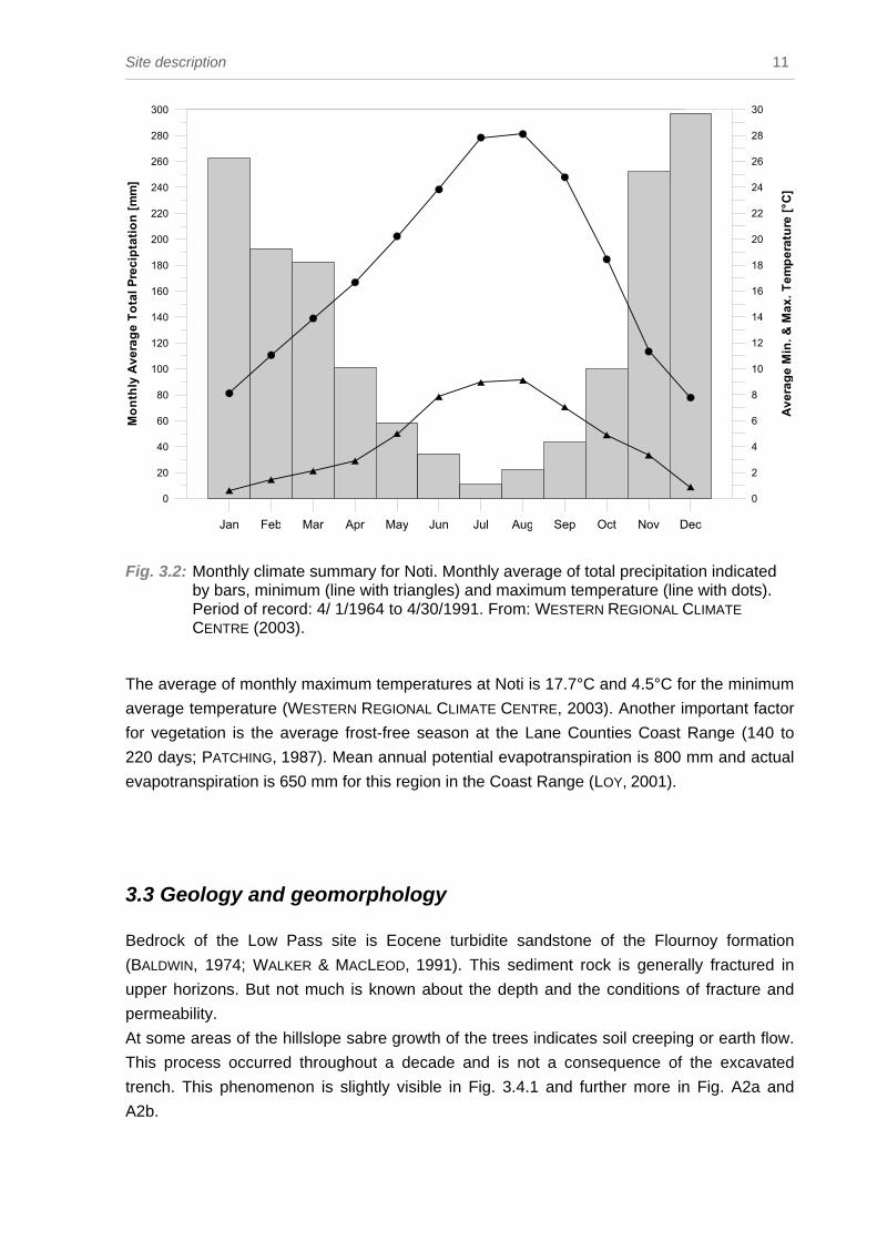
A high seasonality of rainfall is detectable for the site (Fig. 3.2). Most of the average annual
precipitation falls between November and March. Note that the intense phase of field
experiments for this study ran from March, 02, 2003 until May, 28, 2003. During very dry
summer conditions the area is endangered because of bush fires.
Site description 11
Jan Feb Mar Apr May Jun Jul Aug Sep Oct Nov Dec
0
20
40
60
80
100
120
140
160
180
200
220
240
260
280
300
Mon
thly
Ave
rage
Tot
al P
reci
ptat
ion
[mm
]
0
2
4
6
8
10
12
14
16
18
20
22
24
26
28
30
Ave
rage
Min
. & M
ax. T
empe
ratu
re [°
C]
Fig. 3.2: Monthly climate summary for Noti. Monthly average of total precipitation indicated by bars, minimum (line with triangles) and maximum temperature (line with dots). Period of record: 4/ 1/1964 to 4/30/1991. From: WESTERN REGIONAL CLIMATE CENTRE (2003). The average of monthly maximum temperatures at Noti is 17.7°C and 4.5°C for the minimum
average temperature (WESTERN REGIONAL CLIMATE CENTRE, 2003). Another important factor
for vegetation is the average frost-free season at the Lane Counties Coast Range (140 to
220 days; PATCHING, 1987). Mean annual potential evapotranspiration is 800 mm and actual
evapotranspiration is 650 mm for this region in the Coast Range (LOY, 2001).
3.3 Geology and geomorphology Bedrock of the Low Pass site is Eocene turbidite sandstone of the Flournoy formation
(BALDWIN, 1974; WALKER & MACLEOD, 1991). This sediment rock is generally fractured in
upper horizons. But not much is known about the depth and the conditions of fracture and
permeability.
At some areas of the hillslope sabre growth of the trees indicates soil creeping or earth flow.
This process occurred throughout a decade and is not a consequence of the excavated
trench. This phenomenon is slightly visible in Fig. 3.4.1 and further more in Fig. A2a and
A2b.

Site description 12
3.4 Soils Doubtless soil properties are the most influential factors in this study. The procedure of soil
characterisation orientated on AG BODEN (1996). It is based on the visible slope face of the
trench below the hillslope (Fig. 3.4a), a cutslope along the forest road near the site
(Fig. 3.4b) and the actual soil cores within the hillslope. The latter result from 16 auger holes
(up to 250 cm deep) for the piezometer installation, distributed over the lower part of the
hillslope in a grid (see Fig. 3.7). The drillings did not reach any bedrock supposing the total
soil depth to be greater.
The soil order for Coast Range soils is that of an Inceptisols, which occurs in humid regions
and have altered horizons which have lost bases or iron and aluminium but retain some
weatherable minerals (UNITED STATES DEP. OF AGRICULTURE, 2003). A closer look at the soil
cores (see Fig. 3.4c) characterised the series Bohannon sandy loam (PATCHING, 1987). This
is a moderately deep, well drained soil, which was formed mainly in colluviums and residuum
derived from sedimentary rocks.
Typically, the surface is covered with a mat of needles, leaves, and twigs about 2.5 cm thick.
The surface layer is dark brown mineral soil with high live root content. This A-horizon is
about 25 cm thick. Distinctive of the top layers of the B-horizon is the loamy sand with sandy-
skeletal properties. That changes with increasing depth towards sandy loam with a
subangular blocky structure. Also characteristic are loess/sand concretions reaching up to
2 mm in diameter. Highly fractured, weathered sandstone is at a depth of 180 cm. Depth to
the weathered bedrock extends > 250 cm.
Moderately rapid permeability characterises this Bohannon soil. Available water capacity is
about 0.09 - 0.2. Water supplying capacity is about 38 cm (PATCHING, 1987). The effective
rooting depth at the site was 50-100 cm.
Detailed information on the individual piezometer core profiles are attached in Tab. A1.1 –
A1.16. Coos Bay soils, where TORRES et al. (1998) and ANDERSON et al. (1997) described
their experiments at Haplumbrepts of the Bohannon series, can be used for comparisons,
although they mentioned that the sandy loam there is free of significant pedogenic structures
that may favour preferential flow. They summarize that burrows and root holes become
significant avenues for bypassing only if rainfall intensities are extraordinary high.
At the trench face, in particular, a lot of macropores were observed. These ranged up to
8 mm in diameter, with visible length up to 20 cm, and covered almost the whole trench face.
An earlier dye tracing experiment of vertical infiltration, in the same vicinity, showed
pathways with a length of 40 cm (M. WEILER, personal communication). A strong occurrence
of macropores was found in upper horizons, where bioturbation is the main cause, followed
by old roots. With greater depth, now in the sandy horizon, shrinking cracks as a result of
saturated and dry conditions in this vadose zone become more important. Abundance of
macropores declined towards a depth of 150 cm, where almost none of those structures
could be identified.

Site description 13
Fig. 3.4a: Soil characterisation. Beside forest road is the trench excavation with visible soil face (cutslope) of hillslope investigated. Photography was taken prior to the installed roof construction.
Fig. 3.4b: Cutslope along the forest road about 200 m further away of the hillslope.
The vertical distance of the picture is 2 m.

Site description 14
Fig. 3.4c: Soil profile of P_B4 up to a depth of 120 cm. Note MUNSELL colour scale 7.5 YR. Soil exceeding 120 cm depth did not show obvious colour variation to this photographed section and is not shown here.
Important features at this site were some prominent, natural soil pipes, occurring within the
soil. Three soil pipes ended at the soil face in the trench and released water. The distance
between these three outlets was several meters (see Fig. 2.5.1) and their alignment was
almost horizontal. The shape and discharge pattern of the soil pipes is explained in Tab. 5.1.
These soil pipes were probably developed from macropores and erosion forces, as
mentioned above (UCHIDA et al., 1999).
A soil moisture characterisation along the trench or rather the visible soil face, shows the
following features: The southern part of the trench (area of soil pipes openings) has
obviously a wet surface. This general pattern is seen in Fig. 3.4.4. where the moss on the
face just above the soil pipes indicates moist conditions. This section was the moistest part
along the whole trench and contrasted to the north section, where the soil is dried out
completely (see Fig. 3.4.1).

Site description 15
Fig. 3.4d: View of trench below hillslope. Note the location of the three soil pipes
indicated by “x” (big one for SP1). The runoff gutters (subsurface flow collectors) did not have any use in this study.
3.5 Vegetation The increase in precipitation from the Pacific towards the Coastal Range divide is the basis
for coastal temperate rain forests, occurring along the North-American west coast
(ELIAS, 1980). However, not many autochthonous forests survived and most are included in
profit-oriented forest management schedules. So is most of the woodland at Low Pass under
the management of the Forest Service, the Bureau of Land Management, or large private
companies. The Oregon State Department of Forestry regulates many of the woodland
practices used within the area (PATCHING, 1987).
Generally the hillslope is covered with a young stand of forest portrayed in Fig. 3.4.1. The
site was harvested and yarded in July 1983 and replanted in 1984 with mostly Douglas fir
(Pseudotsuga menzeisü). Other species were western red cedar, and salal. The vegetation
on ground, hinted in Fig. 4.1 is dominated by sword fern (Polystichum munitum) and alder
(Alnus spec.). The density of the canopy differs naturally with the some included light spots.
Another feature is the existence of buried and semi buried branches and trees in the soil
vegetation layer. These extended up to 1.2 m in diameter, and are remnants of former
logging actions.
Site description 16
3.6 Overview of the hillslope site The hillslope selected is a zero-order watershed or a headwater. The width of the
investigated site is 30 m and upslope length ranges from 64 m (south) to 114 m (north),
compare Fig. 4.1b. The probable drainage area of the soil pipes, or even an area of
watershed, could not be determined explicitly. Instead, a maximum contribution area was
calculated (see section 4.5.4).
The maximal vertical difference of the selected area is 60 m and the mean slope amounts to
21%. The general topographic pattern of the hillslope shows a concave hollow topography
along the width. This site would be expected to have many confluent flow paths, a situation
that might support flow path studies. Further the lengthwise topography shows a steeper
bottom and a flattening out towards the ridge. The main part of hillslope is located above the
forest road. A map of the hillslope plus the capture of the first order stream is shown in
Fig. 4.1b.
3.7 Conclusions The mountainous hillslope at Low Pass site in the Coast Range is predestined for the
hydrological study of subsurface flow. Aforementioned characteristics of mostly lateral
occurring macropores and presumably in some ways horizontal aligned soil pipes enhance
the interest of studying the connection of these doubled domain preferential pathways.
In order to allow comparisons with other hillslopes where soil pipes occur, findings from the
Low Pass site can be integrated in a wide range of results already presented (e.g. Toinotaini
zero-order valley watershed in UCHIDA et al. (1999) or other a Coast Range site in TORRES et
al. (1998)).
Methods 17
4 Methods This chapter particularly shows the major field methods, the methods at the experimental
hillslope table, the tracer experiments, the data analysis, and finally gives a brief summary of
the basics of laboratory work. It also outlines some of the innovative technical installations
which successfully drove process for the investigations at the hillslope table.
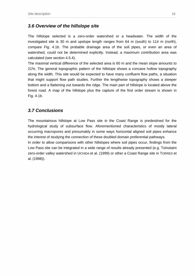
4.1 Field methods Here, a description of the field methods, mostly on measurements techniques used at Low
Pass site is provided. For a picture of the most centred installations see Fig. 4.1a. Note the
black pipes in the back which delivered pipe flow to the tipping buckets (metallic boxes). After
tipping the water ran along the diagonal pipe towards a white bucket. This is where the
bromide probe is slightly visible at the very left edge in the picture. The three remarkable
tubing and bottle units belong to the automatic sampling setup. For general orientation the
map in Fig. 4.1b shows an overview of various instrumentations and the features of the field
site.
Fig. 4.1a: Overview of instrumentation around data logging unit at Low Pass field side.

Methods 18
Fig. 4.1b: Overview on investigated hillslope with instrumentation and extended catchment of a first order stream. Note that the isolines of the selected area show higher resolution because of internal survey. Piezometers are assigned by alpha- nummerical identification codes.
Methods 19
The installation of a trench at the bottom of the hillslope enabled more precise observations
of soil processes. This approach for the detection of subsurface flow mechanisms was
described by WOODS & ROWE (1996) and various others. The vertical face (1.8 m high and
30 m long) was cut across the toe of the hillslope by a power shovel and backhoe. In this
way the soil pipes were excavated in a formerly moist area along the forest road. The cut did
not smear the surface structure of the soil face too much. In order to protect the surface and
to supply a proper discharge sampling of the soil pipes the whole trench was covered by a
plastic roof construction (Fig. 3.4.4). Any observations of the face after rain events (change in
soil moisture, wetting increase) were easier to make under the roof’s shelter.
4.1.1 Determination of precipitation The experimental hillslope is forested with a 19 year old mixed population of coniferous and
deciduous species (see section 3.5). Here, open land precipitation differed from the effective
precipitation reaching the soil because of interception. For Douglas fir stands (NW America
at 45° Latitude) studies have shown 24% interception loss of gross precipitation, for Douglas
fir and others 32%, and for Douglas fir and hemlock 34% (DINGMAN, 2002; ROTHACHER,
1963). Although these values represent old-growth stands, there is still an interception loss
for young stands situated at the field site.
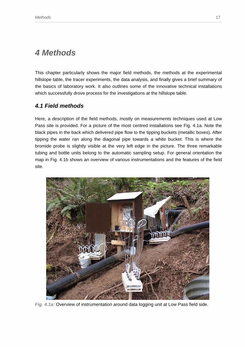
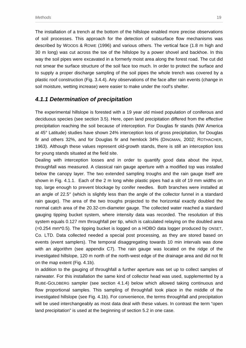
Dealing with interception losses and in order to quantify good data about the input,
throughfall was measured. A classical rain gauge aperture with a modified top was installed
below the canopy layer. The two extended sampling troughs and the rain gauge itself are
shown in Fig. 4.1.1. Each of the 2 m long white plastic pipes had a slit of 19 mm widths on
top, large enough to prevent blockage by conifer needles. Both branches were installed at
an angle of 22.5° (which is slightly less than the angle of the collector funnel in a standard
rain gauge). The area of the two troughs projected to the horizontal exactly doubled the
normal catch area of the 20.32-cm-diameter gauge. The collected water reached a standard
gauging tipping bucket system, where intensity data was recorded. The resolution of this
system equals 0.127 mm throughfall per tip, which is calculated relaying on the doubled area
(=0.254 mm*0.5). The tipping bucket is logged on a HOBO data logger produced by ONSET,
Co. LTD. Data collected needed a special post processing, as they are stored based on
events (event samplers). The temporal disaggregating towards 10 min intervals was done
with an algorithm (see appendix C7). The rain gauge was located on the ridge of the
investigated hillslope, 120 m north of the north-west edge of the drainage area and did not fit
on the map extent (Fig. 4.1b).
In addition to the gauging of throughfall a further aperture was set up to collect samples of
rainwater. For this installation the same kind of collector head was used, supplemented by a
RUBE-GOLDBERG sampler (see section 4.1.4) below which allowed taking continuous and
flow proportional samples. This sampling of throughfall took place in the middle of the
investigated hillslope (see Fig. 4.1b). For convenience, the terms throughfall and precipitation
will be used interchangeably as most data deal with these values. In contrast the term “open
land precipitation” is used at the beginning of section 5.2 in one case.
Methods 20
Fig. 4.1.1: Throughfall gauging below canopy layer of mixed forest.
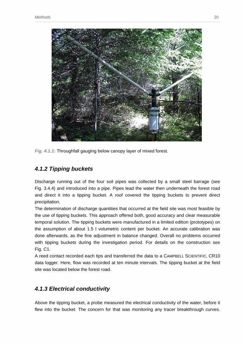
4.1.2 Tipping buckets Discharge running out of the four soil pipes was collected by a small steel barrage (see
Fig. 3.4.4) and introduced into a pipe. Pipes lead the water then underneath the forest road
and direct it into a tipping bucket. A roof covered the tipping buckets to prevent direct
precipitation.
The determination of discharge quantities that occurred at the field site was most feasible by
the use of tipping buckets. This approach offered both, good accuracy and clear measurable
temporal solution. The tipping buckets were manufactured in a limited edition (prototypes) on
the assumption of about 1.5 l volumetric content per bucket. An accurate calibration was
done afterwards, as the fine adjustment in balance changed. Overall no problems occurred
with tipping buckets during the investigation period. For details on the construction see
Fig. C1.
A reed contact recorded each tips and transferred the data to a CAMPBELL SCIENTIFIC, CR10
data logger. Here, flow was recorded at ten minute intervals. The tipping bucket at the field
site was located below the forest road.
4.1.3 Electrical conductivity
Above the tipping bucket, a probe measured the electrical conductivity of the water, before it
flew into the bucket. The concern for that was monitoring any tracer breakthrough curves.
Methods 21
This probe was built after sketch by CAMPBELL SCIENTIFIC and contained a temperature
corrected ohmmeter with a PT 100 thermistor in its core. There was found just little deviation
of 5 µS/cm to a commercial, standard conductivity device. For details on the wiring and
construction see appendix C5. The gauged data water temperature and electrical
conductivity were stored with a CAMPBELL SCIENTIFIC data logger. In this study the storage
module recorded an average of ten minutes.
4.1.4 Automatic sampling setup The collection of water samples after the tracer application was an essential part of the
experiment. Besides taking manual samples at the soil pipes, a continuous sampling of the
discharge was prepared. RUBE-GOLDBERG samplers are simple to produce, have low costs,
and are also well functional and automatic. The most favourable advantage is their direct
dependence on discharge quantities. This pattern is necessary for any calculation of tracer
mass. Such a setup was installed at the outflow of the tipping buckets. Out of the set of three
tipping buckets and sampling units, outlined in Fig. 4.1a, just one set was delivered by water
from the soil pipes. The water ran out of a bucket onto a flow splitter (pipe with a tiny opening
on its convex top). The small diameter allowed 1.5 ml (about 1/1000 of total content tipping
bucket) to enter the pipe which ran towards the first bottle of the automatic sampler. One
bottle’s capacity within a series of six was 270 ml. If this amount had passed through, the
next bottle was filled automatically. For an illustration of the RUBE-GOLDBERG sampler see
Fig. 4.1a. Full sampling bottles were replaced by new ones every day (at the start of the
experimental period) and every seventh day (towards the end).
4.1.5 Bromide probe
The constant monitoring for bromide concentrations was done with a ion-sensitive bromide
probe, manufactured by INSTRUMENTATION NORTHWEST, Inc., Kirkland, USA. It is a
TempHion Submersible Water Quality Sensor called T2, built in 1998 (INW, 2003). This ion
specific electrode (ISE) works based on direct potentiometry, which means that there are two
electrodes that read simultaneously, one sensing electrode and one reference electrode
(submersed in the silver chloride filling solution). These two electrodes act like a dry cell
battery, where the measurement is made after there is difference between the two
electrochemical "half-cell potentials." The NERNST-equation is used to determine half-cell
potential of the sensing electrode, given a stable reference potential (provide by the AgCl);
then that was temperature compensated. All of the equations assume activity of bromide
and not concentration. The installation needs to be vertical, why it was placed inside a
bucket, where outflowing water of the tipping buckets constantly ran through. An additional
shelter prevented algae growth caused by radiation. The monitored data was stored by a
CAMPBELL SCIENTIFIC data logger every ten minutes.

Methods 22
4.1.6 Piezometer Right from the start piezometers were seen as a key tool on the hillslope study. The
distribution of piezometers over the hillslope is concentrated in the lower section, closer to
the trench and the soil pipes. The installation had one first row closely parallel to the trench
and three more following, the last of which had a distance of 35 m to the trench. The grid
arrangement of the piezometers is presented in Fig. 4.1b and exact locations are attached in
Tab. A1.1 to A1.16. From now on the abbreviations tell about the location (row and number
of the piezometer, e.g. P_A5; see Fig. 4.1b)
The initial core hole for the piezometer was made by a hand drill of 8 cm diameter. Drilling
and drawing up the particular soil profile are done simultaneously. An extension enabled to
reach depths of 250 cm, although this could not be achieved at all spots because of local
bedrock formation. In those conditions the minimum achieved was 110 cm. After completion
of drilling, surrounding PVC-pipes were fitted into the hole. As this application focused on
water tables in the saturated zone, the arrangement of slits in the PVC-pipe is just in the
lower part. See appendix C2 for further information.
The recording of water table height in the soil was achieved by installation of a piezometer in
the PVC-pipe. Water table recorders WT-HR, produced by TRUTRACK, Co. LTD, New
Zealand were installed. Further details on this tool provides appendix C2. In this study
averages of 10 minutes were recorded.
Finally the successfully installed piezometers were tested on their connection by a slug test.
An analysis of slug test data offered the calculation of the hydraulic conductivity using the
method of BOUWER & RICE (1980). The method can be used on semi-confined aquifers that
receive most of their water from leakage from the upper confining bed and unconfined
aquifers. The solution is based on the THEIM-equation and assumes negligible drawdown of
the water table around the well and no flow above the water table. The solution is described
by the following equation:
e
twec yyrRrK
L t 2)ln()ln( 0
2
= (E. 4.1.6a)
where: K = hydraulic conductivity [m/s]
rc = radius of well section where water level is rising [m]
Re = effective radial distance over which the head difference y is
dissipated [m]
rw = radial distance between well centre and undisturbed aquifer
(rc plus thickness of gravel envelope) [m]
Le = height of perforated, screened, uncased or otherwise open section
Of well through which ground water enters [m]
yo = y at time zero [m]
yt = y at time t [m]
t = time since y0 [s]

Methods 23
Additionally the simplest interpretation of piezometer recovery is that of HVORSLEV (1951),
which was used for comparisons:
e
wec rLrK
L t 2)ln(2
=
(E. 4.1.6b)
where: see above
4.1.7 Suction cup lysimeter The purpose of these was to sample the draining water in different soil depths. The available
sampler constructions offered either ceramic suction cups or in-situ lysimeters (constructed
from fibre glass cylinders). According to WEBSTER et al. (1993), both showed same bromide
tracer concentrations for a sandy loam. But contrary to these findings indifferent phosphor
concentrations (4.6 times higher) were found in lysimeters than in Teflon suction cup
samplers for a macroporous layered sandy soil (MAGID et al., 1992).
However this study goes along with the first one and so totally six suction cup samplers were
distributed along the hillslope. In the following no distinguishing is done between the different
terms mentioned above.
The soil water samplers (Model 1900) were manufactured by SOILMOISTURE EQUIPMENT
CORP., Santa Barbara, USA. The method of suction cup samplers was reviewed extensively
by LITAOR (1988). They are simple but do provide important insight into the infiltration
process. One clustered arrangement, consisting of three lysimeters, was located just below
the line source tracer application while the other one is within the first row of piezometers
measuring tracer applied over the area (see Fig. 4.1b). Hence, both are referred as either
upper lysimeter (L_U) or bottom lysimeter (L_B). Each set contained soil water samples of
30, 50, and 70 cm depths in order to focus on a tracer gradient and its temporal movement
through the soil. Thus giving an idea how far the tracer went. Further details and a figure of
the lysimeter are attached in appendix C4.
The time ahead the first sampling was 9 days (which is less) to settle the new erected
lysimeter. For the collection, a vacuum between 50 and 60 kPa was created by using a
vacuum test pump with a dial gauge. ANDERSON et al. (1997) and LUXMOORE (1981) used a
suction vacuum of 8.5 kPa in particular for mesopores, although the gradient drives water
from a wider range of pore sizes. Of course pressure head is somewhat arbitrary. No
significant difference in the composition of soil-water solutes was found by BEIER & HANSEN
(1992) when they compared a 40 kPa falling head vacuum with a continuous vacuum of 10
kPa. Therefore no systematic error was seen in the 50 to 60 kPa used in this study under the
assumption of sampled pore sizes < 5 µm.
After the vacuum was applied, the closed pinch clamp sealed the sampler under these
conditions. This caused the moisture to move from the soil through the porous ceramic cup
into the lysimeter. During the experiment the intervals for the suction time were set to

Methods 24
24-48 hours. ANDERSON et al. (1997) used a time step of 6 – 20 h. However this longer time
step provided an integrated sample over the time and avoided water samples too small. The
required quantity for the analysis was 20 ml; this would have been more difficult to achieve in
some drier periods with smaller intervals, just set up on the particular sampling visits. On the
other hand a smaller time interval would provide more exact information. To remove the soil
water sample from the piezometer a plastic tube, a two-hole rubber stopper, a flask or bottle
and the vacuum hand pump were used. Before and after each sample collection, the tube
and the bottle were rinsed twice with deionised water.
4.1.8 Mini v-notch weir For the first order stream a weir was installed and a related catchment proposed. Generally
the triangular shaped weir of Fig. 4.1.8 stated below was installed for additional information
on the understanding of whole hillslope response to rain events. At this low altitude in the
gully, most of the hillslope’s runoff was assumed to pass by. This enhances the descriptive
data on the initial stream related to the runoff processes at preferential pathways at the soil
pipes.
The advantage of the flume installation, instead of another tipping bucket, was an easy and
quick installation. Especially in gauging discharge of smaller quantities they offer accurate
results. The shape of the opening is a “v”-notch with an angle of 60°. The water height in the
notch was recorded by a water height recorder WT-HR, mentioned earlier in this section.
Data is arranged in 10 min intervals. In general, uncertainties of the flume are larger than the
one of the tipping bucket, measuring the soil pipes. Although the data logger had a one mm
resolution, high maintenance was required in this forested catchment to receive confident
data. Any branch being in a cleft stick at the “v”-notch resulted gauge errors. So the data
processing needed much effort. Most obvious single errors were corrected manually. Some
remaining data were not corrected due to uncertainties of true or false data. Further details
on the weir and the discharge calculation are discussed in appendix C3.

Methods 25
Fig. 4.1.8: Flume with WT-HR water height recorder.
4.1.9 Soil moisture probes At a representative location of the hillslope three soil moisture probes were installed in 30, 50
and 70 cm soil depth. Unfortunately, there occurred a battery error with a loss of major data.
A reason here fore was the high required voltage for the three probes connected to the same
battery supply. This problem was solved with an installed 12 V battery instead of one with a
smaller capacity. The series of available data is very restricted and does not allow expressive
conclusions to be presented here. For further information on the installation and technical
details see section 4.2.6.
Methods 26
4.2 Experimental hillslope table Artificial, physical experiments in science demand to simulate the natural processes.
Although the simplified approach can not capture the entire complexity of natural systems
there is still evidence about the gained process understanding. To achieve perfect identity
between natural processes and simulation must fail. Moreover the goal is merely to get best
possible reflection of the natural processes, particularly as hydrologic modelling is most
credible when it does not pretend to be too sophisticated and all inclusive (KLEMEŠ, 1986).
Runoff development on hillslope scale is complex and often includes a combination of
several processes. Regarding the physical modelling the outstanding difficulty is to arrange
the soil structure at the experimental setup in its original pattern.
4.2.1 Table itself Performing experiments on an artificial hillslope table needs a particular geometrical affinity
to truth hillslopes. The dimensions were 198 cm width, 395 cm length and 20 cm depths (18
cm effective soil depth). Unchanneled headwater basins often show roughly about these
three dimensional ratios (GUTKNECHT, 1996; TORRES et al., 1998). Most important in this
study was the similarity of the Low Pass field site and the experimental table. The length and
width there for the more detailed section was about 40 x 80 m, and the approximate soil
depth until the bedrock showed at least 2.4 m. Another affinity was the slope. Following the
Low Pass field site, the tables slope was set to 25% (respectively 14°) to provide similar
environments.
The presented Fig. 4.2.1 shows the table, including the soil filling and the nozzles of the rain
simulator. The black plastic nearby the table helped to minimize the errors of spray, where
the irrigation failed the table. This error was very little, but nevertheless was collected by the
galvanized gutters. On the soil, little tubes belonging to the little water sampling wells (see
section 4.2.5). Furthermore a black cable is visible which belongs to a soil moisture sensor,
buried underneath.
The base of the table was a heavy steal frame with four legs. Above, the basin (rectangular
parallel piped) was lined out with smooth PVC boards and sealed properly. The outflow side
wall contained wire netting (mesh size: 2 mm) over the full width, where the water was able
to pass through. Then water was divided into eight chambers (sediment trapping), which
each contributed towards a tipping bucket. See Fig. 4.2.3a for the arrangements of tipping
buckets.

Methods 27
Fig. 4.2.1: Artificial hillslope table and rainfall simulator. Note that the centred gutter does not fit into the setup, this is a protection against splash effects on the soil from nozzles after the run.
4.2.2 Soil filling
Filling up the empty table was presumably the major challenge within the work on the
experimental hillslope. Natural conditions of soil features at the field side are most subtle and
change a lot. The detailed transfer of structures, developed throughout many years to an
artificial hillslope, using manpower and a shovel is impossible. Outstanding changes find
expression in soil density, water holding capacity, predefined pathways for water, etc.. A
literature review on soil packing found very less records about the filling for bigger volumes,
whereas much was found for soil columns and porous groundwater aquifer modelling
(OLIVIERA et al., 1996).
It is apparent, that a raining method with free falling sand passing through a sequence of
sieves before reaching the surface of the sand body was used at different groundwater
experiments (STAUFFER & DRACOS, 1986). In general literature elucidated two different ways
of filling the soil in order to get close to original conditions. One is described by wet filling.
Here the sand is washed in, most suitable the sand water blend runs through a hose. For this
process gravity is less dominant, which causes a different particle distribution and erection of
layers. The wet sand is dried out afterwards. The other way is dry filling (OLIVIERA et al.,
1996).
However, as this study had to deal with loamy sands instead of homogeneous sand, things
were more difficult (YARON et al., 1966). Soil physiologists, who were included into the

Methods 28
question, recommended the dry filling technique. Here, theory incorporates a reduction of
velocity for heavy soil lumps. This is commonly achieved by a designed construction of a
vertical pipe with horizontal nails in randomly chosen arrangements throughout the length of
the pipe. This little tool has great similarities to a ‘rain stick’ manufactured by the aborigines.
The effect is a slow down of soil lumps, which does provide a homogenous soil arrangement
in both, area distribution and soil depth profile.
In contrast to the recommendations the “delaying tool” could not be used for these
experiments because of the loamy soil of the Low Pass site. Most of the soil was dense
compacted. The actual distribution of the soil was undertaken by a rake, levelling layer after
layer. No additional procedure was used to adapt soil density. The major concern about the
soil treatment was to aware surface runoff. Therefore a minimal micro relief with tiny raked
contours (plowing structures) was added on the top of the surface. The dry soil bulk density
of the table was determined at two representative locations and varies around
1.1 g/cm.
4.2.3 Rain simulator
A rain simulator triggered the artificial rain for the table. Inflow quantities running in from the
tab were measured by a flowmeter (accuracy: ± 0,378 l) at the tab. Sprinkling used water
from the public water supply which was not demineralised. The simulator consisted of seven
nozzles, fixed on a moving guide rail which moves along the length of the table. This was
forced by an electrical, linear accelerator (rotating spindle). The brass nozzles sprinkled
minute drops in a spraying angle of 100° towards the soil. The nozzles had an adjacent
distance (centre to centre) of 40 cm. The elongation of the guide rail was equal to the
distances of the nozzles; this means no overlapping of the spraying. As the motor moved
linear, stopped at the end and returned linear no periodically distribution (e.g. sine function)
traced the spray (WEILER, 2001). The impact energy of the produced sprinkle was small
except for the time after the simulator was switched of and the remaining water run out. For
those events a separate gutter was used.
To prevent undefined losses at the borders, a black plastic collected the spray-induced
variations. The error of evaporation was assumed to be negligible. The finally deposited rain
within five minutes was investigated in a test phase by nine beakers (diameter 5 cm) spread
out at the table on a 3x3 matrix. Later these values were extrapolated to hourly intensities.
The result showed lengthwise uniform artificial rainfall with a little asymmetric pattern along
the width of the table (see Fig. 4.2.3b). Summarizing this pattern is defined as too small to
result any influence on the goal of this study. The overall mean was 38 mm/hr, meaning on
this hourly basis (although these experiments applied 5 and 10 min intervals). This intensity
(on 1 hour duration) has a return period of about 100 years at the Oregon Coast Range
(GOARD, D.L., in prep.).

Methods 29
The triggering of irrigation intervals relayed on the prevention of surface runoff. The irrigation
rate for the table remained in 5 min on- followed by 10 min off-intervals. Towards the very
end of the investigation the sprinkling quantity was raised up and a few runs took 10 min rain
followed by a 10 min break.
0 20 40 60 80 100 120 140 160 180
0
20
40
60
80
100
120
140
160
180
200
220
240
260
280
300
320
340
360
380
Width of table [cm]
Leng
th o
f tab
le [c
m]
Fig. 4.2.3a: Shape of table, dividing for collection chambers of tipping buckets (vertical strings), piezometers (points), soil moisture sensors (E) and location of
sampling wells (crosses).

Methods 30
0 20 40 60 80 100 120 140 160 180
Width of table [cm]
0
5
10
15
20
25
30
35
40
45
50
55
60
Sprin
klin
g in
tens
ities
[mm
/h]
0
5
10
15
20
25
30
35
40
45
50
55
60
cross section y= 227.5 cmcross section y= 167.5 cmcross section y= 77.5 cm
Fig. 4.2.3b: Distribution of sprinkling intensities (mm/hr) along different transects of table.
4.2.4 Tipping buckets at table
The discharge quantities at the hillslope table are different from those in the field. While
planning the experiment the same blueprint as for the tipping buckets in the field was scaled
down to a volumetric content of 75 ml (see appendix C1). However, the small tipping buckets
were arranged in a series of eight, to provide discharge measurements over the total transect
of the tables outflow. A couple of problems raised from the downscaling of the tipping
buckets and had to be solved. First, the weight of the bucket was heavy in relation to the
weight of water. Second, the friction within the axis made accurate tipping initiation of the
buckets impossible. However the problems could be solved by using ball bearings and going
ahead with a general tuning. So, installation of the contact switch was modified and updated.
After fine adjustments, the rating was investigated for the eight tipping bucket as a mean of
80 tips. Finally the volumetric content ranged from 53 -89 ml for the particular buckets (mean:
70 ml/tip). Final data went to a CAMPBELL SCIENTIFIC data logger, stored by sums over two
minutes. Tipping bucket one (TB1) is on the left hand side of the table and captures the width
0 -22.5 cm. Tipping bucket eight (TB8) is at the end of the series at 173.5 -198 cm (see
Fig. 4.2.3a).

Methods 31
4.2.5 Mini-wells for water sampling Measuring tracer concentrations directly in the soil water was an important concern because
this provided more detailed information on the movement of the tracer through the soil. For
the spatial investigation of the line source tracer application (see section 4.3.2), twelve
mini-wells were installed in a grid, shown in Fig. 4.2.3a. The constructional challenge for the
mini-wells in the soil was high, in order to be aware of any rapid water passing by vertical
closely. The sampling should exclusively include water from the lower centimetres of the soil
layer. Therefore the construction is similar to the piezometers in the field with an additional
suction pipe in the centre, which allowed the sampling of small water quantities out of the
bottom close zone with a syringe. These small volumes were important in three ways: First,
to keep as much water in the system as possible; second, to obtain real time samples, no
former tracer concentration had firstly to be flushed out (amount of water) before taking the
samples; third, low disturbances of the soil system. All constructional features are
documented in appendix C7. The sample interval for these twelve mini-wells was 15 minutes.
4.2.6 Piezometers at table The arrangement of piezometers at the table was different from that in the field. Furthermore
the setup might be special, even for the first time described. The initial challenge was to
establish a mechanism to get water table data within the shallow soil of the table (height
18 cm) without minimal interference. To be aware of any sprinkling water bypassing the
piezometers, the decision went towards a minimal impact approach. Therefore a hole in the
bottom of the table allowed pressure transmission in a connecting hose. This hose is
permanently filled with water and ran towards a water level recorder WT-HR (previously
mentioned in section 4.1.6). The connection between hose and WT-HR was established with
some garden hoses and silicon work (Fig. 4.2.6). So the water height in the table and in the
piezometer was connected by the hose. It was assumed simplistically that the water table
within the soil matrix is equal to the non-soil conditions (plain column of water). This was the
case as reference measurements were too difficult to obtain, although there were indicating
data from the ECH2O probes (see later) about the soil moisture content. Medical gauze
(bandage available at pharmacies) serves function of sediment protection at the entrance on
the bottom of the table. The piezometers were arranged in four rows by each three (Fig
4.2.3a). This grid distribution was sufficient for the investigated phenomena of spatial water
tables. The distance between the outflow and the piezometer rows was 77.5, 167.5, 227.5
and
298 cm. Out of totally 12 piezometers just two did not response properly after water table
establishing. This was caused by either a clog up at the start of the hole of the table, or by
any non-equal soil condition or lack of water from leaking at the PVC pipe and its
connections. The data was recorded in two minute intervals.
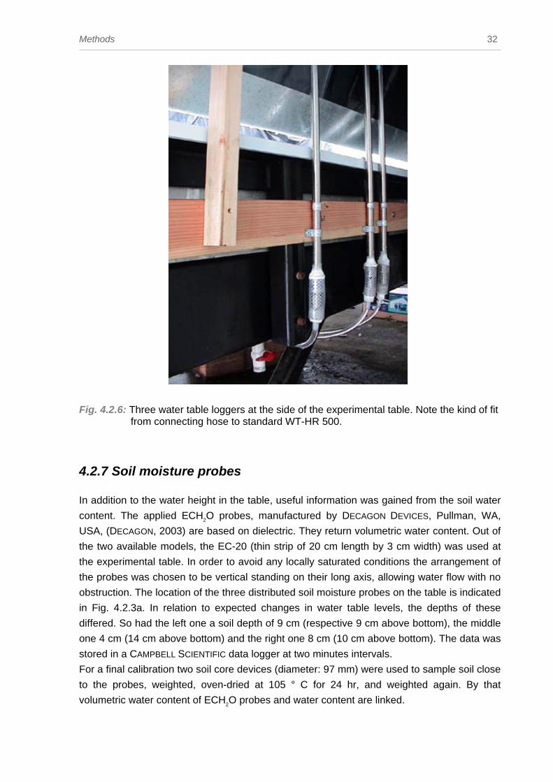
Methods 32
Fig. 4.2.6: Three water table loggers at the side of the experimental table. Note the kind of fit from connecting hose to standard WT-HR 500.
4.2.7 Soil moisture probes In addition to the water height in the table, useful information was gained from the soil water
content. The applied ECH2O probes, manufactured by DECAGON DEVICES, Pullman, WA,
USA, (DECAGON, 2003) are based on dielectric. They return volumetric water content. Out of
the two available models, the EC-20 (thin strip of 20 cm length by 3 cm width) was used at
the experimental table. In order to avoid any locally saturated conditions the arrangement of
the probes was chosen to be vertical standing on their long axis, allowing water flow with no
obstruction. The location of the three distributed soil moisture probes on the table is indicated
in Fig. 4.2.3a. In relation to expected changes in water table levels, the depths of these
differed. So had the left one a soil depth of 9 cm (respective 9 cm above bottom), the middle
one 4 cm (14 cm above bottom) and the right one 8 cm (10 cm above bottom). The data was
stored in a CAMPBELL SCIENTIFIC data logger at two minutes intervals.
For a final calibration two soil core devices (diameter: 97 mm) were used to sample soil close
to the probes, weighted, oven-dried at 105 ° C for 24 hr, and weighted again. By that
volumetric water content of ECH2O probes and water content are linked.
Methods 33
4.3 General information on the applied tracer
It is primarily proclaimed that concentration dimensions of parts per billion (ppb) equals
µg/litre.
Bearing in mind the goal of soil water tracing, the decision in this study went towards the use
of two artificial tracers. In general, specific investigations in the unsaturated zone are
confronted with the high potential of sorption. First, Amino G Acid was applied as a
fluorescent dye tracer for a line application in the ground, second was a salt tracer for the
extensive distribution on the hillslope (vegetation cover close to the surface). Both Amino G
Acid and bromide are commonly used in unsaturated zone studies (SCHUDEL ET AL, 2003;
FEYEN et al., 1999). For general information on fluorescence tracer and analysis see
SCHUDEL ET AL, 2003; MIKOVARI et al., 1995). No proof was found about interfering of bromide
and Amino G Acid as co-tracers (whereas e.g. lithium bromide and Rhodamine do; JONES &
JUNG, 1990).
For experimental runs at the hillslope table, those two tracers were applied, too. However,
the bromide was added to the sprinkling water, an easier and clean way to do. To obtain
further information on the flow paths the third tracer experiment contained a Brilliant Blue
FCF line source application. Now, separate viewing follows:
Line Source: Amino G Acid (Techn: 7-Amino-1,3 Naphthalenedisulphonic Acid
Monopotassium Salt)
Amino G Acid belongs to the group of functionalized polycyclic aromatic hydrocarbons.
Various productions are available (e.g. CAS # 86-65-7, 842-15-9). For this study a
composition with CAS # 842-15-9 by ACROS ORGANICS, Fair Lawn, New York was used. The
appearance of the substance is almost white powder and the molecular weight comes to
341.4 g/mol.
Fluorescence tracers are easy to handle, simple to detect and rapid to analyse quantifiably
using fluorometer techniques. Here, an exposure or an excitation with light reacts in the
tracer’s light emission peak of particular wave length afterwards. This pattern is significant
for the substance. SMART & LAIDLAW (1977) report 355 (310) nm for maximum excitation and
445 nm for maximal emission wavelength. However, BEHRENS (1986) reported 359 nm for
maximum excitation and 459 nm for an approximate maximal emission wavelength. This
appeared to be closer of different productions. Emission spectra in our analysis showed
peaks at 455 nm in the fluorometer. Using an emission peak set to 455 nm, there two
excitation peaks occurred in the fluorescent spectrum at 310 (large peak) and 350 nm
(smaller).
The chemical structure of Amino G Acid is shown in Fig. 4.3.1a.
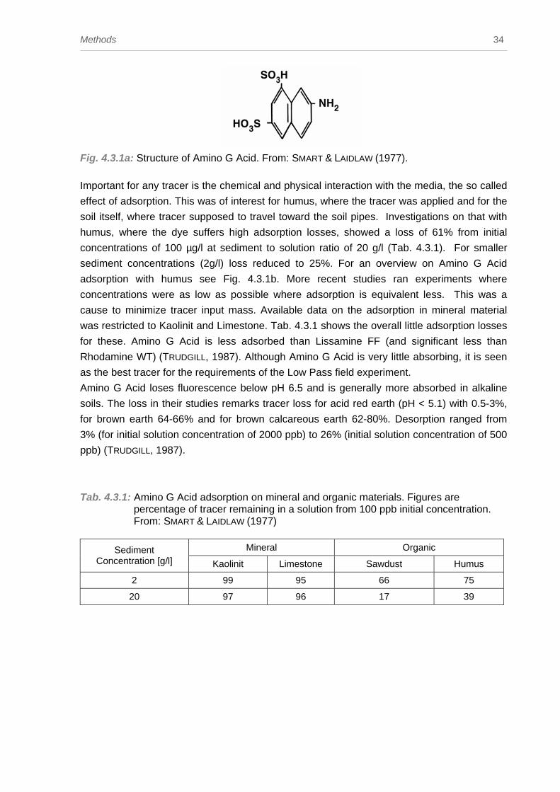
Methods 34
Fig. 4.3.1a: Structure of Amino G Acid. From: SMART & LAIDLAW (1977).
Important for any tracer is the chemical and physical interaction with the media, the so called
effect of adsorption. This was of interest for humus, where the tracer was applied and for the
soil itself, where tracer supposed to travel toward the soil pipes. Investigations on that with
humus, where the dye suffers high adsorption losses, showed a loss of 61% from initial
concentrations of 100 µg/l at sediment to solution ratio of 20 g/l (Tab. 4.3.1). For smaller
sediment concentrations (2g/l) loss reduced to 25%. For an overview on Amino G Acid
adsorption with humus see Fig. 4.3.1b. More recent studies ran experiments where
concentrations were as low as possible where adsorption is equivalent less. This was a
cause to minimize tracer input mass. Available data on the adsorption in mineral material
was restricted to Kaolinit and Limestone. Tab. 4.3.1 shows the overall little adsorption losses
for these. Amino G Acid is less adsorbed than Lissamine FF (and significant less than
Rhodamine WT) (TRUDGILL, 1987). Although Amino G Acid is very little absorbing, it is seen
as the best tracer for the requirements of the Low Pass field experiment.
Amino G Acid loses fluorescence below pH 6.5 and is generally more absorbed in alkaline
soils. The loss in their studies remarks tracer loss for acid red earth (pH < 5.1) with 0.5-3%,
for brown earth 64-66% and for brown calcareous earth 62-80%. Desorption ranged from
3% (for initial solution concentration of 2000 ppb) to 26% (initial solution concentration of 500
ppb) (TRUDGILL, 1987).
Tab. 4.3.1: Amino G Acid adsorption on mineral and organic materials. Figures are percentage of tracer remaining in a solution from 100 ppb initial concentration. From: SMART & LAIDLAW (1977)
Mineral Organic Sediment Concentration [g/l] Kaolinit Limestone Sawdust Humus
2 99 95 66 75
20 97 96 17 39

Methods 35
0 2 4 6 8Humus Concent
10ration [g / l Dry Weight]
0
20
40
60
80
100
Perc
enta
ge o
f Ini
tial F
lour
esce
nce
Fig. 4.3.1b: Adsorption of Amino G Acid on humus sediment. Initial concentrations were
100 ppb. From: SMART & LAIDLAW (1977).
Background fluorescence of Amino G Acid at brown calcareous earth for streams shows 20-
100 ppb and for suction cups 200-800 ppb (TRUDGILL, 1987). Amino G Acid is subject to
photochemical decay over a period of days. Thus dye solutions should be shielded from light
before use and during collection and analysis. The photochemical decay for a setup of
100 µg/l exposed six hours during sunny conditions amounted to a decay coefficient of
1.6 E-2. The same concentration for the same time under a 60 W lamp got a decay
coefficient of 3.7 E-4 (SMART & LAIDLAW, 1977). A covering of heavy duty polythene is
recommended for water sampling apparatus.
No column test or batch test was performed with the soil at Low Pass field site in order to get
better information on the sorption of this particular soil.
Extensive application: Bromide
The use of bromide in hydrology takes advantage of the circumstance that bromide does not
occur naturally in most of catchments (FLURY & PAPRITZ, 1993). Bromide in not included in
the nutrient cycle and there is no intake of micro organisms. Therefore excellent conditions
for the detection of the tracer are provided. Concluding, bromide is considered as a
conservative tracer in mineral soil (FLURY et al., 1995); Although there is evidence that in
humic soil layers anion adsorption might occur (LANGE et al., 1996).
For these experiments a lithium bromide solution was used, manufactured by FMC
CORPORATION, Bessemer City, New York (product CAS number: 7550-35-8). The purity of
the colourless liquid is 75-80% (calculated with 77.5%) and the molecular weight equals
86.84 g/mol.

Methods 36
Line Source: Brilliant Blue FCF
For the line source the food dye Brilliant Blue FCF (CAS # 42090; N-Ethyl-N-[4-[[4-[ethyl[(3-
sulfophenyl) methyl]amino]phenyl](2-surfophenyl) methylene]-2,5-cyclohexadien-1-ylidene]-
3-surfobenzenemethanaminium hydroxide inner salt, disodium salt; C37H34N2Na2O9-S3) was
used. It adsorbs weakly on soils but in relation to Amino G Acid it has a stronger isotherm
sorption (FLURY & FLÜHLER, 1995). But due to its low toxicity, high visibility and high mobility
it is one of the best compromises available up to date as dye tracer to visualize flow the
pathways in vadose zone (GERMÁN-HEINS & FLURY, 2000; WEILER, 2001). Any tracing
experiments with Brilliant Blue have the recommendation of high concentration input to
ensure that the dye is still visible after adsorption. In this study they were employed to
provide quantitative results on the covered distance of tracer movement.
4.4 Characteristics of the tracer experiments The tracer input mass determination had the philosophy of a minimal impact in the system.
Any positive record of tracer should not and is not allowed to be obtained by an excessive
tracer input mass. Further, as the solution ratio is limited for substances a smaller input mass
needs smaller quantities of water. This aspect is not to neglect for smaller systems like the
hillslope table. A rough estimation of tracer input mass was done considering the following
factors: lowest detectible tracer concentration in the outflow, expected time between injection
and arrival of the peak, size of the soil volume that will be involved in transporting the tracer,
water content of the soil and finally expected pipe flow. Another approach to calculate tracer
input mass is provided by LEIBUNDGUT & WERNLI (1984):
6 E2f AdcQCt
⋅⋅⋅⋅⋅
=TIM (E. 4.4)
where: TIM = tracer input mass [kg]
t = estimated time of tracer break through [h]
C = max. concentration at sampling site [mg/m³]
Q = pipe flow [m³/h]
Adc = adsorption coefficient [-]
f = factor of safety [-]
But still any calculation of tracer input mass is to be treated as assumption as the variables
rely on the characteristic results explored by the experiment.
The tracer applications of bromide and Amino G Acid were conducted simultaneously in each
of the study locations.

Methods 37
Line Source: Amino G Acid
Despite several available formulas, which allow to calculate the dimension of input mass
experience is also needed for the determination of tracer input mass. We included weather
forecast data and based our calculation on a simple assumption of an upcoming event
similar to ID 2+3. A first approach estimated mass to 150 g (see Tab. A4) and a second
using E. 4.4 got about similar results. For the latter an adsorption factor of 0.3 was included
and also the advice of SCHUDEL et al. (2003) who suggest for experiments in the unsaturated
zone a double to triplet tracer input mass in relation to saturated conditions (implicated in
factor of safety). Thus for the in-line application at the field site on April, 2 an input mass of
150 g was applied. This was seen as a representative value, which was in the range of
similar experiments (MCGUIRE, personal communications). For the hillslope table experiment
water volumes were calculated in the table using soil volume and drainable porosity. Further,
a peak concentration of 150 ppb was aimed to prevent sorption losses. The finally applied
tracer input mass amounted to 0.1 g.
The subsurface line source was applied at the field site in a virtual line, indicated in Fig. 4.1b.
Here injections of 20 ml were set each 20 cm. At the table the line (length: 100 cm) was
located centred in the width of the table at a distance of 285 cm from the outflow. Concerning
the humus layer in the field of about 5 cm the tracer injection had to be in this depth, as
sorption reduces without organic matter (see above). In both cases needles, fitting to the
front of medical syringes were used for the injection. Needles got clocked up every now and
then by soil particles and were replaced. Beside that, the method is very clean and does
shield from contamination in a good way. Prior to injection no pre-wetting was done!
Extensive application: Bromide
Here, determination of input mass relied on a maximal concentration of 10000 ppb and the
portion of initial mobilisation was assumed to be 100% for the spraying of the area (Tab. A4).
For the application at the field site on April, 2 a total quantity of 8 kg bromide diluted into
50 l was sprinkled close above the soil cover over the hillslope. For the proceeding of manual
sprinkling a spray gun and a pressure canister (used at planting or crop spraying) rendered
the service. The nozzle outflow was regulated for an equal distribution of the 50 l and
achieved a constant spray. To avoid spraying overlap in the forested, dense vegetated
environment little amount of Brilliant Blue FCF was added to the transparent solution. With
that a visible check helped to distinguish between zones already sprayed and zones with
spraying to go. The sprayed area is shown in Fig. 4.1b and was of course selected by the
spatial proximity to the outlet of soil pipes. The application area was 493 m².
The hillslope table experiment used 5 g bromide in liquid phase. This was placed in a tool to
admix fertilizer (available at farmers supply), which is screwed in between tab and the hose.
As the water ran through, it gathers proportionate bromide. It was assumed that all of tracer
mass was delivered towards the nozzles within the initial irrigation interval of 5 min.

Methods 38
Line Source: Brilliant Blue FCF
The line source of Brilliant Blue FCF was restrictively applied at the table. It was the third and
final tracer experiment as the sampling required excavation of soil. The tracer input mass of
100 g was diluted by 500 ml deionised water (about the maximum solubility). This liquid was
applied in the same procedure than the Amino G Acid with syringes. The centred line of
100 cm length had a distance of 290 cm to the outflow.
Sampling and analysis in general
All water samples were collected in HDPE bottles. Water samples at the weir, the soil pipes,
the lysimeters and the piezometers were collected daily (beginning) to 4th-daily (towards the
end of the study).
Samples were stored below 4 °C until the analysis. The unfiltered samples were settled a few
days, to deposit the little sediment. The detection of Amino G Acid was done with a TURNER
DESIGNS Model 10 AU fluorometer. Only a couple of samples were influenced by clouding or
higher background concentration. Unfortunately interfering by the cork, used to seal the
glasses, occurred at some samples. Using this aperture the detection limit was 5 ppb.
The analysis of the bromide samples is processed with a DINONEX 2000 ion chromatograph.
This process required a filtering of the samples, as a lot of the field samples contained
sediment. The execution of that is managed by a suction filtering aperture and paper filter.
This process also needed extra care as the cleaning with deionised water is of major
importance. According to the lack of time the parts were rinsed twice and reused directly
again, without air drying of the glassware. Some of the samples bottles were already filtered
with GEHLMANN GHP Acrodisc 0.45 µm, located on top of a syringe. The detection limit of
bromide in an ion chromatograph was at 1 ppb.
Electrical conductivity was used as a tool to monitor bromide breakthrough at the soil pipes
runoff. The increase of electrical conductivity (EC) is well connected to the increase of
bromide concentration, as the mean natural conductivity at the hillslope is very low (previous
long range mean: 40 µS/cm) and no other artificial intake occurred. For the final
determination of bromide concentration in the flow continuous measurements of EC were
combined with the hand samples with laboratory based bromide determination.
4.5 Data analysis Centre of mass
The distribution of rainfall can be wide spread with many events over the time interval
investigated. To get a referring point for the analysis the temporal gap between rainfall and
runoff, the centre of mass was determined for the rainfall distribution. This was calculated
based on daily values, for intervals including several days and in the other case for single
day events based on 10 minutes values.

Methods 39
Seven day antecedent precipitation index, API7
Previous studies at the Oregon Coast Range suggested the integration of antecedent rainfall
characteristics under conditions of low intensity rainfall to predict the amount of runoff
(ISTOK & BOERSMA, 1986). This index is also a helpful indirect indicator on soil moisture. This
calculation was done as a simple summation rather than a weighting summation as
described by MANIAK (1997). The daily totals of the seven days before a hydrograph rise
were included. Amounts of precipitation as well of API7 were rounded to integer values.
Hydrograph separation
For a simplified separation of base flow the start of event flow in the hydrograph was set at
the hydrographs obvious rise. The determination of the events ending point contained more
difficulties. Even the easiest way by using an empiric formula (e.g. LINSLEY) must fail as the
catchment area is not known. More common methods focus on the different storage
coefficients of fast and slow responding components (DYCK & PESCHKE, 1995). Here, the
obvious change of slope or turning point in the recession curve of the hydrograph tells about
the ending point of the event. A visual check of the graphs, plotted in a semi logarithmic
scale was done for a hydrograph separation on event components and base flow
components. The final separation was achieved with a direct connecting line of the starting
point and the end point (trapezoid). In this case the shape of hydrograph did not allow any
detection of a turning point, a horizontal line starting at the rise of flow did the separation
towards the ending point (result: rectangle).
Timing of flow
The time shift of flow is calculated between the rainfalls centre of mass and the runoff peak.
The time to flow includes the time between the rainfalls centre of mass and the start of flow.
This index is positive for following runoff reaction and negative in case the start of flow is
ahead the rainfalls centre of mass.
Recession analysis
In order to determine turnover times and storage feature recession branches are analysed on
the assumption of a single linear reservoir by the MAILLET-formula The event series were
selected on condition that three to four days ahead didn’t get any rainfall and the series until
the next rise of discharge contained at least five days. These strong demands on the data
were performed following base flow investigation methods (DYCK & PESCHKE, 1995). Results
are presented individually and are not combined to a master recession curve.
Runoff coefficient
Index is calculated as follows:
PR d=ψ (E. 4.5a)

Methods 40
where: � = runoff coefficient [-]; 0 � � � 1
Rd = direct runoff, stormflow [mm]
P = precipitation [mm]
Dynamic contributing area of soil pipes
An approach for an arithmetic estimation of the drainage area of a soil pipe lead back to
DICKINSON & WHITELEY and CALVER et al. (both in JONES, 1997). A first step towards is a
base flow separation (already explained in the previous chapter). The formula then offers the
calculation of a surrogate ‘catchment area’ based on the maximum contributing area. These
were selected from the dynamic contributing area (DCA) for each storm, according to:
rainfall storm totalpipein discharge storm total
=DCA (E. 4.5b)
This is based on a runoff coefficient of 1.0 in a given storm. It is a summarised calculation for
all three soil pipes, for sure with a dominating representation of SP1. The authors there
recommend a large sample size of about 20 complete storm records. As this study does not
have such this formula can not ensure a reasonably representative result.
Velocities of tracer experiment
The description of a black box system with tracer techniques uses relevant parameters,
which are presented in the following. Various velocities are determined of the tracer break
through curve:
maxmax t
x=aV (E. 4.5c)
peak tx
=peakaV (E. 4.5d)
med tx
=medaV (E. 4.5e)
minmin t
x=aV (E. 4.5f)
where: x = Distance between input and sampling location [m]
ta max = Time between input and first tracer contact [s]
ta peak = Time between input and concentration maximum [s]
ta med = Time between input and median [s]

Methods 41
ta min = Time between input and end of tracer break through [s]
Tracer recovery rate
The calculation of the relative tracer recovery rate at time t is:
∫=t
dttCtTRR0
)(MQ)( (E. 4.5g)
where: Q = discharge [l]
M = mass of tracer [g]
C(t) = tracer concentration at time t [g/l]
4.6 Conclusions Most of the methods applied in the research at this Low Pass field site are common and
widely used in experimental hydrology. The Low Pass field site was well equiped with
instrumentation in order to achieve the objectives of the study. The best choice of tracer
regarding conditions at the field site was made on bromide and Amino G Acid because of
their sorption characteristics and their use in soil water tracing.
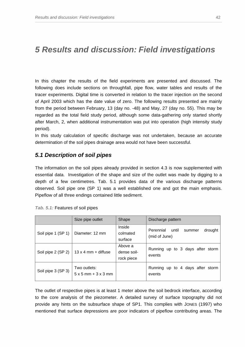
Results and discussion: Field investigations 42
5 Results and discussion: Field investigations In this chapter the results of the field experiments are presented and discussed. The
following does include sections on throughfall, pipe flow, water tables and results of the
tracer experiments. Digital time is converted in relation to the tracer injection on the second
of April 2003 which has the date value of zero. The following results presented are mainly
from the period between February, 13 (day no. -48) and May, 27 (day no. 55). This may be
regarded as the total field study period, although some data-gathering only started shortly
after March, 2, when additional instrumentation was put into operation (high intensity study
period).
In this study calculation of specific discharge was not undertaken, because an accurate
determination of the soil pipes drainage area would not have been successful.
5.1 Description of soil pipes The information on the soil pipes already provided in section 4.3 is now supplemented with
essential data. Investigation of the shape and size of the outlet was made by digging to a
depth of a few centimetres. Tab. 5.1 provides data of the various discharge patterns
observed. Soil pipe one (SP 1) was a well established one and got the main emphasis.
Pipeflow of all three endings contained little sediment.
Tab. 5.1: Features of soil pipes Size pipe outlet Shape Discharge pattern
Soil pipe 1 (SP 1)
Diameter: 12 mm
Inside
colmated
surface
Perennial until summer drought
(mid of June)
Soil pipe 2 (SP 2)
13 x 4 mm + diffuse
Above a
dense soil-
rock piece
Running up to 3 days after storm
events
Soil pipe 3 (SP 3)
Two outlets:
5 x 5 mm + 3 x 3 mm
Running up to 4 days after storm
events
The outlet of respective pipes is at least 1 meter above the soil bedrock interface, according
to the core analysis of the piezometer. A detailed survey of surface topography did not
provide any hints on the subsurface shape of SP1. This complies with JONES (1997) who
mentioned that surface depressions are poor indicators of pipeflow contributing areas. The
Results and discussion: Field investigations 43
data on discharge presented mainly involves water running out of SP 1, since SP 2 and SP 3
started up only in wet conditions.
No interflow occurred at the soil face in the trench throughout the study. For the already
moist conditions in the southern part of the trench (area of soil pipes), the additional visible
wetness after rain events was very small. However, this wetness of the surface was still not
enough to produce seepage. Hence, outflow in the soil profile under investigations (to a
depth of 1.8 m) was totally restricted to the soil pipes. Previously constructed gutters to
collect interflow, shown in Fig. 3.4.4, were not involved as they appeared to be useless.
Discussion of soil pipe features
A similar observation where pipe flow was responsible for 95% of the outflow of a small
granitic headwater and almost no interflow occurred was reported by TSUMAMOTO et al.
(1982). The observations of the site made in Tab. 5.1 show that the pipe outlet seemed not
to be located close to the soil bedrock interface (MCDONNELL, 1990) or within a narrow band
above the soil bedrock interface (UCHIDA, 2002). The results go more along with a study in
north-coastal California where pipe outlets occur near the soil surface to a depth of about
2 m and are commonly situated at gullies or sinkholes (ZIEMER & ALBRIGHT, 1987). More
precise information about the shape and location of the soil pipes might be possible using
ground-penetrating radar, as HOLDEN et al. (2002) did in peat soil. This may also provide
data about the depth of soil-bedrock interfaces. A fibrescope examination on morphologic
features was not undertaken, but provides potential to detect triple-junctions
(TERAJIMA et al., 2000).
5.2 Precipitation Before presenting the data measured at the hillslope, the general context of the investigation
period is analysed. Because of annual variations, the winter 2002/2003 got less precipitation
than in the long-range mean. Available data of the long-term climate station Eugene (see
Fig. 3.1) are shown in Fig. 5.2a. This had an influence on the long-term water balance of the
field site Low Pass with effects on the results of the soil pipe study.

Results and discussion: Field investigations 44
10/02 11/02 12/02 01/03 02/03 03/03 04/03 05/03
0
50
100
150
200
250
300
350
Mon
thly
pre
cipi
tatio
n [m
m]
Monthly precipitation, long-term meanRecent monthly precipitation
Fig. 5.2a: Open land precipitation at the climate station Eugene, for overall investigation
period (October 2002 to May 2003) and long-term mean. From: OREGON CLIMATE SERVICE (2003).
After this general context, the data of the throughfall measurement at the hillslope itself are
presented: Despite a data gap around day -3, the hillslope received a total throughfall of
392 mm for the period February, 13 (day no. -48) to May, 14 (day no. 42). Decreasing of
rainfall towards summer, mentioned in section 3.2, is traceable by the negative trend of daily
values. Daily measurements of precipitation are presented in Fig. 5.2b. Daily totals reached
up to 51 mm. Summarising daily values in amounts of multiple days (e.g. pacific fronts
passing through) helped with the analysis. Those were calculated as sums between days
with no rain. Therefore, Tab. 5.2 presents rainfall data for time intervals, which range
between 16 and 131 mm and showed resulting flow events.
Changing the objective from daily amounts to smaller time steps, for example 10 minutes, an
analysis of events focuses on intensity. Here, a mixture of mostly low rainfall intensities
interspersed by some high spikes was obtained. The maximal intensities are listed in the
third column of Tab. 5.2 for a series of selected intervals. The maximal intensity observed
was 5.2 mm/10 min (equals 32 mm/hr), followed by 2.83 mm/10 min (equals 17 mm/hr). The
context of the second peak, as well as general variation of intensities are shown in Fig. 5.2c.
Furthermore the API7 is provided in Tab. 5.2 for events, as an indirect indicator on soil
moisture. This value will be used in section 5.3 about flow to relate responding runoff start
with its rain conditions seven days before.

Results and discussion: Field investigations 45
-50 -40 -30 -20 -10 0 10 20 30 40No. of days, relative to tracer application on April, 2
0
20
40
60
80
100
120
140
160
180
200
220
240
260
280
300
Dis
char
ge s
oil p
ipes
[ l /
10
min
]
ID1
ID2ID3
ID4
ID5 ID6
ID7
60
50
40
30
20
10
0
58565452
48464442
38363432
28262422
18161412
8642
Thro
ughf
all P
reci
ptat
ion
[ mm
/ da
y ]
-50 -40 -30 -20 -10 0 10 20 30 40
ThroughfallDischarge soil pipes
Fig. 5.2b: Daily rainfall at field site Low Pass and pipe flow (addition of SP1, SP2, SP3) for
study period.
-45 -44 -43-45.75 -45.5 -45.25 -44.75 -44.5 -44.25 -43.75 -43.5 -43.25
No. of days, relative to tracer application on April, 2
0
10
20
30
40
50
Dis
char
ge s
oil p
ipes
[ l /
10m
in ]
3
2.5
2
1.5
1
0.5
0
Thro
ughf
all P
reci
ptat
ion
[ mm
/ 10
min
]
-45 -44 -43-45.75 -45.5 -45.25 -44.75 -44.5 -44.25 -43.75 -43.5 -43.25
ThroughfallDischarge soil pipes
Fig. 5.2c: Rainfall intensities per 10 min for selected interval, additionally hydrograph
(pattern of tipping buckets).

Results and discussion: Field investigations 46
Tab. 5.2: Selected characteristic of rainfall and runoff attributes for the hillslope and pipeflow. Note the relation between rain interval and peak ID, a reason to merge the two table parts Rainfall; section 5.2 Runoff; section 5.3
Rain
dominated
interval
[day no.]
Pre-
cipitation
[mm]
Max.
intensity
[mm/10
min]
API7
[mm]
Peak
ID
Total
event
pipe flow,
without
base flow
[m³]
Peak
flow
soil
pipes
[l/10min]
Time
shift:
rain
to
flow
[hr]
Time to
start of
flow
[hr]
-46 to -43 31 2.83 gap 1 74 60 38 26
-28 to -24 100 1.03 8 2+3 446 150 28 -3
-14 to - 8 131 1.75 8 4+5 760 258 27 -7
0 to 4 16 0.74 gap 6 152 98 61 46
8 to 10 19 0.68 14 - - - - -
21 to 24 40 0.99 10 7 87 35 47 14
39 22 5.2 3 - - - - -
Discussion of precipitation
The precipitation event on day 39 became a little suspicious as the distribution of 10 min-
intensities clarified. A large intensity of 5.2 mm/10 min occurred at the very first time step of
the event on that day and afterwards intensities went down to about 1.5 mm/10 min. But also
a check on one of the additional open area precipitation recorders (closely located) showed
the same outstanding intensity and daily amount. Thus the data seems to be correct. In order
to get an idea about the rainfall occurred that day, a look on nearby climate stations at
Eugene city and Alsea fish hatchery revealed 0.5 and 0 mm respectively (OREGON CLIMATE
SERVICE, 2003; G.H. TAYLOR, personal communication). Two Stations further away (Corvallis
city and Guin Library Weather Station at the Hatfield Marine Science Centre in Newport,
Pacific Coast) recorded daily totals of 7 mm respectively 0 mm (AGRIMET, 2003; HATFIELD
MARINE SCIENCE CENTRE, 2003). Although the gradient of rainfall in this luv-lee system is
superposed by another pattern, it was conducted: Considering the amount of rainfall of 22
mm with a maximal intensity of 5.2 mm/10 min (equals 32 mm/hr), on day 39 surrounded by
low rainfall amounts, indicates a very locally extended convective storm cell with a heavy
burst.
Despite this maximum the dominant low rainfall intensity observed is characteristic for the
Coast Range, as ISTOK & BOERSMA (1986) found that intensities of 12.71 mm/hr were
exceeded very rarely.
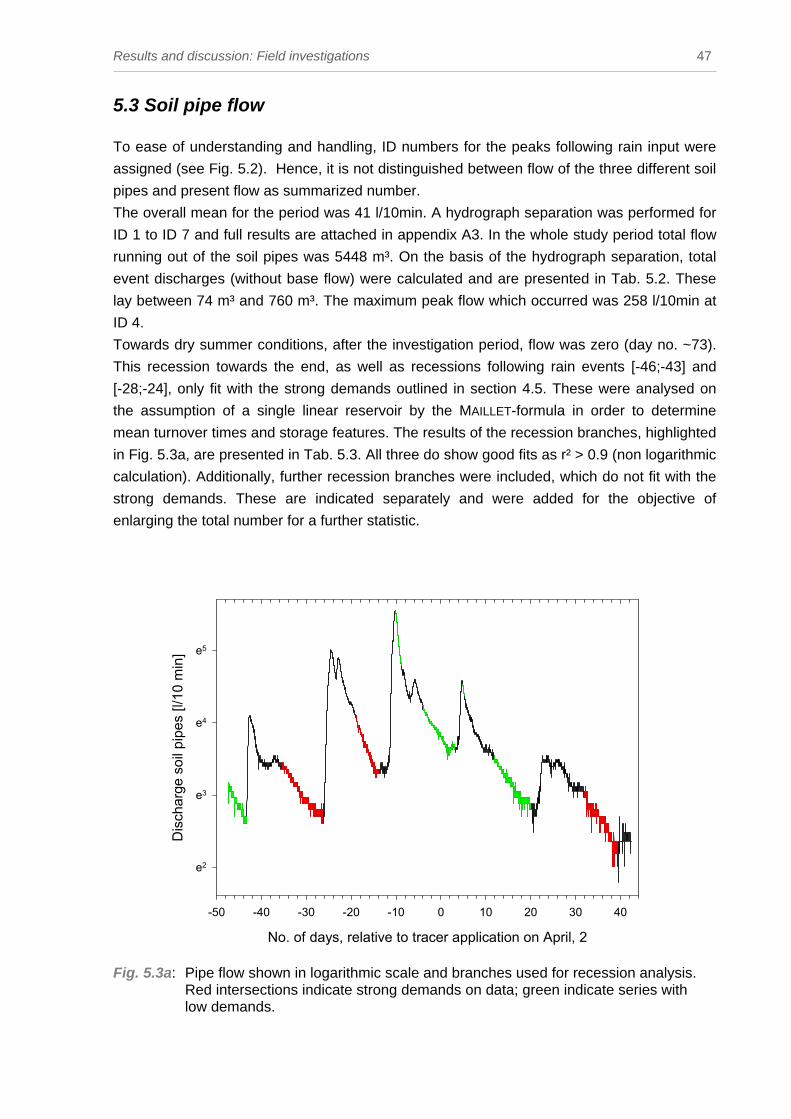
Results and discussion: Field investigations 47
5.3 Soil pipe flow To ease of understanding and handling, ID numbers for the peaks following rain input were
assigned (see Fig. 5.2). Hence, it is not distinguished between flow of the three different soil
pipes and present flow as summarized number.
The overall mean for the period was 41 l/10min. A hydrograph separation was performed for
ID 1 to ID 7 and full results are attached in appendix A3. In the whole study period total flow
running out of the soil pipes was 5448 m³. On the basis of the hydrograph separation, total
event discharges (without base flow) were calculated and are presented in Tab. 5.2. These
lay between 74 m³ and 760 m³. The maximum peak flow which occurred was 258 l/10min at
ID 4.
Towards dry summer conditions, after the investigation period, flow was zero (day no. ~73).
This recession towards the end, as well as recessions following rain events [-46;-43] and
[-28;-24], only fit with the strong demands outlined in section 4.5. These were analysed on
the assumption of a single linear reservoir by the MAILLET-formula in order to determine
mean turnover times and storage features. The results of the recession branches, highlighted
in Fig. 5.3a, are presented in Tab. 5.3. All three do show good fits as r² > 0.9 (non logarithmic
calculation). Additionally, further recession branches were included, which do not fit with the
strong demands. These are indicated separately and were added for the objective of
enlarging the total number for a further statistic.
No. of days, relative to tracer application on April, 2
-50 -40 -30 -20 -10 0 10 20 30 40
Dis
char
ge s
oil p
ipes
[l/1
0 m
in]
e2
e3
e4
e5
Fig. 5.3a: Pipe flow shown in logarithmic scale and branches used for recession analysis. Red intersections indicate strong demands on data; green indicate series with low demands.

Results and discussion: Field investigations 48
Tab. 5.3: Recession analysis of selected events and storage coefficient of the system
Rain event
ahead
[Day no.]
Demand
on
data
Corres-
ponding
peak ID
Coefficient α of
MAILLET-formula teQtQ ⋅−⋅= α
0)(
[1/d]
Regression
coefficient,
r²
[-]
Storage coefficient
k,
mean turnover
time Rt_
α1_
== Rtk
[d]
Mean
discharge
over
recession
branch
[l/10min]
-47.3 to -43.4 low - 0.013 0.92 76 18
-46 to - 43 high 1 0.014 0.94 69 25
-28 to - 24 high 2+3 0.043 0.97 23 44
-10 to -8.8 low 4 0.774 0.97 1 176
-4 to 3 low 5 0.029 0.93 34 48
4.84 to 5.2 low 6 0.259 0.97 4 87
12 to 20 low 6 0.013 0.93 77 23
To interpret this information table, it is important to know that the mean turnover time chiefly
provides information on the dynamic of the system. For true residence time tracer information
depending on the mobile phase is required. Now the extraction of table information shows:
During low flow conditions at the soil pipe (flow < 25 l/10min), storage coefficients greater
than 69 days illustrate the slow outflow out of the system and imply a slow dynamic. For the
event [-28;-24] the amount of water in the system is different as the second highest
discharge peak occurred just some days ahead of that recession. Runoff then was still
quickly driven and different fluxes were active during this mean discharge of 44 l /10 min (see
Fig. 5.2b). For the enlarged number of events investigated, the dependence of mean
turnover time on mean discharge is presented by a linear recession analysis (generalisation
of the MAILLET-formula) in Fig. 5.3b. This graph shows the pattern of quick turnover times for
high mean discharge conditions, whereas the dynamic of the system is slow for small
discharges. As the recession time constant varies systematically with discharge, there is a
consistency with a nonlinear storage-discharge model.

Results and discussion: Field investigations 49
Mean turnover time [d]
0 10 20 30 40 50 60 70 80 90 100
Mea
n di
scha
rge
[l/10
min
]
e2
e3
e4
e5
r ² = 0,88
r2= 0.88
Fig. 5.3b: Recession of mean discharge over recession branch and mean turnover time for selected events outlined in Tab. 5.3.
5.3.1 Timing of soil pipe flow and flux
The time shift between rainfall and runoff ranges from 27 to 61 hours for the events selected
in Tab. 5.2. Plotting the time shift against the precipitation quantity showed a negative linear
trend (R²= 0.74). Although harder to detect, a focus on the start of flow instead of peak flow
showed delay times of -3 to +46 hours. Negative times occurred here in case of wide spread
rainfall distribution with double peaks, then start of flow was ahead of the centre of mass in
rainfall.
The response of soil pipe flow volume to a given quantity of precipitation was variable and
depended on API7 (listed in Tab. 5.2) representing the total water content of the system.
Here, the total number did not allow conclusions on any dependence.
5.3.2 Discussion of soil pipe flow
General: To set up a water balance for the study period is hard to achieve as the investigation period
remains short, respectively shorter than a hydrological year. A short term comparison for the
investigation period of total flow (5448 m³) with total throughfall (392 mm) is linked to the

Results and discussion: Field investigations 50
uncertainty of an unknown catchment area. The issue of catchment area will also be
discussed in section 5.4.
A look at the rain events [0;4] with 16 mm of rain and [8;10] with 19 mm of rain surprised
because of the different reaction they generate. In one case a discharge of 148 m³ is
prominent compared with no obvious reaction for the even bigger, second event. This seems
to be the start of the dryer system conditions, which got more obvious on day 39, when no
system response at all occurred after heavy rainfall input. Although for an annual series,
compareable results were obtained at a similar Oregon Coast Range site, where 44% to 93%
of all the rainfall events produced no measurable runoff (ISTOK & BOERSMA, 1986).
The results of Fig. 5.3b are distinct from processes relevant to DARCYs law where turnover
times would not change for different mean discharges. A highly heterogenic system, with a
runoff generation mechanisms that differ from DARCYs law is summarized. This is in
particular because those processes are valid within cm-scale, but not within a scale of
decametre, to be assumed here. Additional different mean discharges in Fig. 5.3b are also
connected to different conditions of water content in the system. Thus turnover times also
represent the hydrologic connection and finally determine the dynamic of the system. Quick
turn-over times for high mean discharge conditions are likely to be interpreted by no water
resistance in wet soil environments or a possible water table. But there is also the possibility
that higher soil moisture produces pressure transmission. The response dependence on
water tables in the hillslope will be shown in section 5.3.
Observations that bypassing preferential flow (respectively pipe flow) became more
important when rainfall intensities were extraordinary high could not be confirmed in this
study (observations at similar soil type by TORRES et al., 1998).
Timing: The phenomena of different lag times in forest soils under wet and dry conditions are widely
described (e.g. TURTON et al., 1992; MCDONNELL, 1990). Generally, the response times
indicated a fast acting mechanism (e.g. Tab. 5.2). Obviously, SP1 acts as a preferred path
mechanism. Similar responses of subsurface flow in forest soils have been observed by
MOSLEY (1982), MCDONNELL (1990) and TURTON et al. (1992) although the latter focused on
subsurface flow in general, rather than a soil pipe mechanism operating.
Concerning lag time and time shift the results here are not very consistent. A comparison of
the events [-28;-24] and [-14;-8] seems difficult. They both had about similar starting
conditions (API7, and total precipitation), which resulted in about the same flow lag time
(3- 7.5 h).
Stepwise multiple linear regression using rainfall amount, API7 and mean intensity as
independent variables and total flow as dependent variable were achieved, but appeared
critical as the total number of events is too small. However, regressions for time shift were
more significant than time to start of flow. These findings go along with ZIEMER & ALBRIGHT
(1987). As well an analysis using SPEARMAN rank order correlation failed because of the
small data total.

Results and discussion: Field investigations 51
The API7 did not help much to explain flow mechanisms as the values were too similar and
the availability low. Conclusions point towards the major importance of the soil water content,
especially the water table rather than the antecedent rain index.
5.4 Dynamic contributing area of soil pipes
The dynamic contributing area (DCA) was calculated in Tab. 5.4 for the events linked to peak
ID, according to equation E. 4.5b. The maximum DCA occurred on peak ID 6. Here,
throughfall showed the smallest value and the border issues of the hydrograph separation
are added in Tab. A3. However, the maximum amounted to 1 ha and the reach of the soil
pipes was assumed to that with already mentioned uncertainties.
Further the table presents runoff coefficients of the different events based on an assumed
catchment area equal to DCA. The average runoff coefficient calculated for the peaks ID 1-5
and ID 7 amounted to 0.375.
Tab. 5.4: Pipe flow records, DCA and runoff coefficients
Rain
dominated
interval
[day no.]
Pre-
cipitation
[mm]
Peak
ID
Total
event
flow,
without
base flow
[m³]
Peak flow
soil
pipes
[l/10min]
DCA
[m²]
according
to
E. 4.5b
Runoff coefficient ψ,
based on max DCA
= catchment area
-46 to -43 31 1 74 60 2387 0.239-28 to -24 100 2+3 446 150 4460 0.446-14 to - 8 131 4+5 760 258 5802 0.5800 to 4 16 6 152 98 9500 max! 121 to 24 40 7 87 35 2175 0.218
Discussion of contributing area
The maximum contributing area amounts at least to 9500 m². Regarding the fact that a runoff
coefficient of exactly one is hard to obtain, the area is presumably bigger. Including the
uncertainties of the hydrograph separation of ID 6 (see appendix A3) the large contributing
area should be treated with scepsis. However, it differs in the order of magnitude from the
bromide sprayed area (highlighted in Fig. 4.1b and section 4.4) with its 493 m², which was
expected primarily to be the contributing area. Finally, even a large DCA does still not
include evidence about the shape and predominant direction of the soil pipes.
For the size of pipe outlet (assumption: SP1 as most dominant feature) the contributing area
seems to be very high. UCHIDA et al. (1999) presented values of 158 m² for a soil pipe
diameter of 5 cm in a similar forested catchment.

Results and discussion: Field investigations 52
A comparison of pipe flow runoff coefficients, based on DCA, shows the same order of
magnitude as the Maesnant basin (� = 0.4), where soil pipes show similar maximum DCA and
quantity of storm flow is comparible (DUNNE, 1978 citied in JONES, 1997). Runoff coefficients
on subsurface flow for the Toinotaini zero-order watershed differ little from the Low Pass
ones (� = 0.24; UCHIDA et al., 1999). However, looking at the magnitude of �, both are still
distinguishable from through flow (� = 0.11 according to DUNNE, 1978 citied in JONES, 1997) by
the higher coefficient. Thus it is another indication that pipe flow here is to be assigned to a
different category.
5.5 Piezometer results The visual check of the slug test results did not show anything suspicious, why the
piezometers were rated well connected to the surrounding soil (Fig. A4). Out of the slug test
data the hydraulic conductivity was calculated (by E. 4.1.6a and 4.1.6b) to 1.4 E-07 m/s
respectively 2.1 E-07 m/s.
5.5.1 Water table levels Data of the water table is presented in depth below surface topography rather than height in
the piezometer drillings. Series are discontinuous because some recorder’s offset was not
deep enough! Tables showed the general pattern of a greater response in lower parts
(piezometer row A) than in higher elevations of the hillslope (piezometer row D), where slope
was higher. Furthermore, even within a row the development was different, for example
piezometer P_A5 to P_A9 had good response to rain events with great amplitude whereas
P_A1 and P_A3 did not. This fact is surprising because it was mentioned earlier that the
southern part of the trench in the neighbourhood of P_A1 had moist trench faces, plus the
mouths of the soil pipes were 2 m below P_A1 and P_A3 and in contrast the other part of
trench face was always dry. Therefore the trench face does not represent wetness in
hillslope behind.
Fig 5.5.1a gives an overview of selected piezometers. The focus is primarily on the water
table variation in interaction with the biggest runoff event ID 4. Here the maximum amplitude
(in relation to the individual offset of each piezometer) occurred at P_A7 with 588 mm
followed by P_C9 with 487 mm (Tab. 5.5.2). Therefore a well responding area is identifed in
that region of P_A7 and P_C7.
Generally the saturation of soil as a post-rainfall process happened in soil depths of up to
80-100 cm (for row A) below surface topography. The saturation zone for upper piezometer
rows was deeper, at about 1.4 m or even around 2.2 m (see Fig. 5.5.1a and
Fig. A5).

Results and discussion: Field investigations 53
-40 -30 -20 -10 0 10 20 30-46 -44 -42 -38 -36 -34 -32 -28 -26 -24 -22 -18 -16 -14 -12 -8 -6 -4 -2 2 4 6 8 12 14 16 18 22 24 26 28 32
No. of days, relative to tracer application on April, 2
-1700
-1600
-1500
-1400
-1300
-1200
-1100
-1000
-900
-800
-700
-600
-500
Wat
er ta
ble
[ mm
bel
ow s
urfa
ce]
-40 -30 -20 -10 0 10 20 30-46 -44 -42 -38 -36 -34 -32 -28 -26 -24 -22 -18 -16 -14 -12 -8 -6 -4 -2 2 4 6 8 12 14 16 18 22 24 26 28 32
0
10
20
30
40
50
60
Thro
ughf
all [
mm
]
0
50
100
150
200
250
Dis
char
ge s
oil p
ipes
[l/1
0 m
in]
API
7- co
ntin
ous
[mm
]
Runoff soil pipesDaily throughfallWater table P_A3Water table P_A5Water table P_A7Water table P_A9Water table P_C7Water table P_C9API 7-continuous
Fig. 5.5.1a: Water table at various piezometers, pipe flow and throughfall. Series of P_C9 includes missing data. Note the different offset of the individual piezometers.
Another observation at P_A9 is the rain event (20 mm) at day minus eight, where under API7
conditions of 109 mm a second peak of the water table was established. Here, the system
responded rapidly because of the already moist conditions. Precipitation input is traceable
throughout water table and discharge data.
Coming back to the water table levels connected to ID 4 a mapping of the different water
levels in the spatial context of the piezometers is performed for the well-responding area
around P_A7 and P_C7. The time steps included showed maximal or minimal levels for at
least one piezometer or any other outstanding feature. Fig. 5.5.1b shows again the
heterogeneity of the piezometers in row A, whereas Fig. 5.5.1c presents row C.
To show the relation between water table height and discharge, correlations were performed.
However, the received hysteresis did not provide much information as discontinuous data
series were included. The pattern of hysteresis is hard to interpret and is attached in Fig. A6.
Therefore, the next section focuses on timing.

Results and discussion: Field investigations 54
6 8 10 12 14 16 18 20 22 24 26 28 30 32 34 36 38
Distance [m]
-1800
-1600
-1400
-1200
-1000
-800
-600
-400
-200
0D
epth
bel
ow s
urfa
ce to
pogr
aphy
[mm
]
-1800
-1600
-1400
-1200
-1000
-800
-600
-400
-200
0
6 8 10 12 14 16 18 20 22 24 26 28 30 32 34 36 38
P_A3P_A5
P_A7
P_A9
Digital time: -10.61
Digital time: -10.28
Digital time: -9.87
Digital time: -0.75
Fig. 5.5.1b: Water table levels at piezometers in row A ahead, while and after ID 4. Piezometer offset is indicated by grey bars.
8 10 12 14 16 18 20 22 24 26 28 30 32 34 36 38
Distance [m]
-1800
-1600
-1400
-1200
-1000
-800
-600
-400
-200
0
Dep
th b
elow
sur
face
topo
grap
hy [m
m]
-1800
-1600
-1400
-1200
-1000
-800
-600
-400
-200
0
8 10 12 14 16 18 20 22 24 26 28 30 32 34 36 38
P_C7
P_C9
Digital time: -12.87
Digital time: -10.87
Digital time: -10.28
Digital time: -0.75
Fig. 5.5.1c: Water table levels at piezometers in row C ahead, while and after ID 4. Piezometer offset is indicated by grey bars.

Results and discussion: Field investigations 55
5.5.2 Timing of water table establishment
Referring to the special features of P_A7 and P_C7 indicated above, the timing of those is
once more significant. Both water table series also show the bigger time lags with the
hydrograph, in comparison with the others. Furthermore, the deviation towards the major
discharge peak on day minus ten is 11 hours ahead for P_A7 and 11 hours back for P_C7.
The time shift for other events is presented in Tab. 5.5.2. The rising time is sometimes hard
to separate as the graphs showed some previous peaks.
Tab. 5.5.2: Data of selected piezometer on selected events, including time shift Piezometer Event
[day-No.]
Corres-
ponding
peak ID
Time shift (peak
hydrograph to peak
water table) [hr];
convention: ⊕ = water
table ahead of
hydrograph
time to
rise
[hr]
Remarks Rise of
water table
[mm]
P_A3 [-24;-23] 3 +6 52 238
[-10] 4 +2.5 70 on top of
recession
branch
181
[5] 6 +1 50 137
P_A5 [-10] 4 -11 27 122
P_A7 [-43;-42] 1 +11 1.9 on top of
recession
branch
316
[-24;-23] 3 +32 15 304
[-10] 4 +11 2.6 588
[5] 6 +19 1.2 on top of
recession
branch
308
P_A9 [-36;-32] - -69 87 further
event on
top
52
[-24;-23] 3 -60 70 74
[-10] 4 -11 76 94
[5] 6 -12 82 76
[24] 7 -81 88 66
P_C7 [-10] 4 -11 35 305
[5] 6 -19 45 28
P_C9 [-43;-42] 1 +11 3.5 449
[-10] 4 +6 30 487
P_C3 [-10] 4 too little 10

Results and discussion: Field investigations 56
response
The pattern of P_A3 shows the smallest time shift between flow soil pipe and water table.
Additionally the shape of the water table graph is similar to the hydrograph
(Fig. A5). This is explained by the proximity of P_A3 and the soil pipes.
Pointing to Tab. 4.4.2 the positive time shift of P_A7 is conspicuous. In relation to the rainfall
input the water table established faster than discharge occurred, a pattern shows in
Fig. 5.5.1.b. This raises the question about the overall dominating process and which is first?
5.5.3 Spatial presentation of water table
Illustrating the spatial distribution of the water table over the hillslope is difficult, as the last
section showed. The heterogeneous response generated by the individual connection of
each piezometer to surrounding groundwater caused problems. These show up in particular
there, where no response occurred. However, the water table was spatially interpolated for
the biggest runoff event (peak ID 4). This seem to be of interest as water tables showed the
biggest amplitudes, with spatially the most expanded water levels, around day no. -10. Data
source were the few piezometer data of Fig. 5.5.1b+c. The calculation included five selected
well responding piezometers (indicated by green crosses) as point values which were
interpolated by the „Inverse Distance Weighting” (IDW) method. This is based on the
assumption that each point value has a local influence, which declines with increasing
distance from the reference (BURROUGH & MCDONNELL, 1998). The area of the applied
interpolation was selected by field experience, data availability and the interpretation of data
presented in the chapter above. Time steps were chosen non-linearly and correspond to the
individual maxima or minima of the different piezometers used and relayed also on the
hydrograph.
The spatial change in water levels over time is presented in Fig. 5.5.3. However, the depth of
water decreases with an expansion of those saturation zones 900 - 700 mm close to surface.
The most extended area with probable highest water levels (and thus water content) is
detected for the digital time -10.6. This development occurred about 12 hours before pipe
flow peak. At that moment the extension had already declined (see digital time -10.2).
Despite the water table at the north part having a wide distribution in a depth of 900 –
700 mm and beeing even wide distributed, no interflow could be seen there (previously
mentioned). The decline in spatial distribution and absolute water level towards time -9.63
and -0.75 is similar contrary to the rise which happened before. Generally, heterogeneity,
side effects, and the interpolation method blur the spatial presentation the most, why Fig.
5.5.1b+c is more clear.
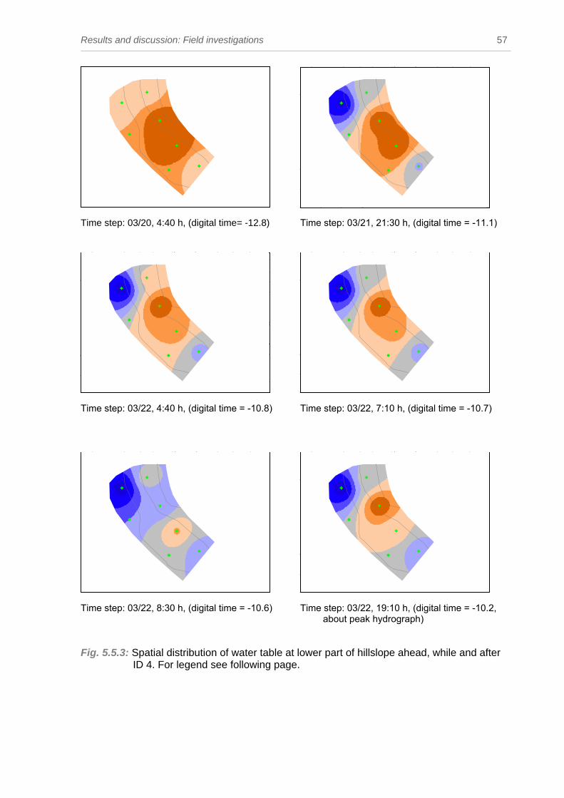
Results and discussion: Field investigations 57
Time step: 03/20, 4:40 h, (digital time= -12.8) Time step: 03/21, 21:30 h, (digital time = -11.1)
Time step: 03/22, 4:40 h, (digital time = -10.8)
Time step: 03/22, 7:10 h, (digital time = -10.7)
Time step: 03/22, 8:30 h, (digital time = -10.6) Time step: 03/22, 19:10 h, (digital time = -10.2, about peak hydrograph)
Fig. 5.5.3: Spatial distribution of water table at lower part of hillslope ahead, while and after ID 4. For legend see following page.
Ñ
Ñ
Ñ
Ñ
Ñ #
#
# #
#
#
#
#
#
Ñ
Ñ
Ñ
Ñ
Ñ #
#
# #
#
#
#
#
#
Ñ
Ñ
Ñ
Ñ
Ñ #
#
# #
#
#
#
#
#
Ñ
Ñ
Ñ
Ñ
Ñ #
#
# #
#
#
#
#
#
Ñ
Ñ
Ñ
Ñ
Ñ #
#
# #
#
#
#
#
#
Ñ
Ñ
Ñ
Ñ
Ñ #
#
# #
#
#
#
#
#
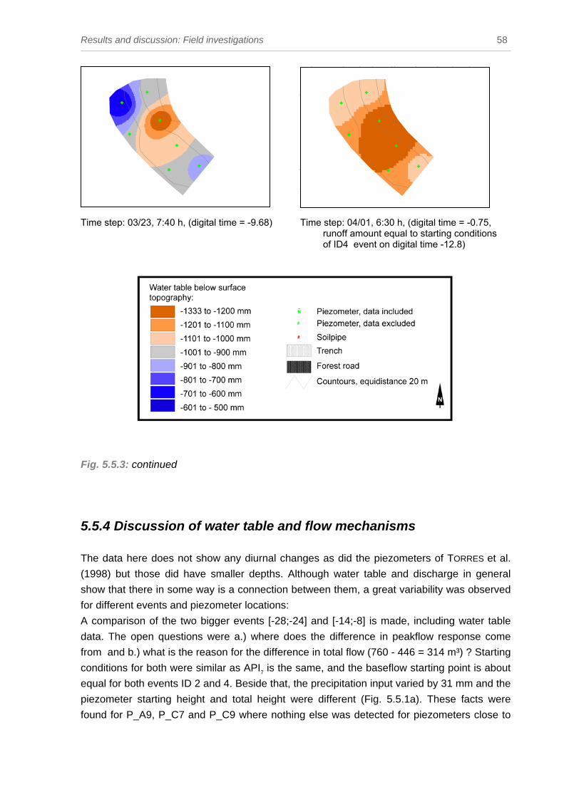
Results and discussion: Field investigations 58
Time step: 03/23, 7:40 h, (digital time = -9.68) Time step: 04/01, 6:30 h, (digital time = -0.75, runoff amount equal to starting conditions of ID4 event on digital time -12.8)
Ñ
Ñ
Ñ
Ñ
Ñ #
#
# #
#
#
#
#
#
Ñ
Ñ
Ñ
Ñ
Ñ #
#
# #
#
#
#
#
#
Fig. 5.5.3: continued
5.5.4 Discussion of water table and flow mechanisms
The data here does not show any diurnal changes as did the piezometers of TORRES et al.
(1998) but those did have smaller depths. Although water table and discharge in general
show that there in some way is a connection between them, a great variability was observed
for different events and piezometer locations:
A comparison of the two bigger events [-28;-24] and [-14;-8] is made, including water table
data. The open questions were a.) where does the difference in peakflow response come
from and b.) what is the reason for the difference in total flow (760 - 446 = 314 m³) ? Starting
conditions for both were similar as API7 is the same, and the baseflow starting point is about
equal for both events ID 2 and 4. Beside that, the precipitation input varied by 31 mm and the
piezometer starting height and total height were different (Fig. 5.5.1a). These facts were
found for P_A9, P_C7 and P_C9 where nothing else was detected for piezometers close to
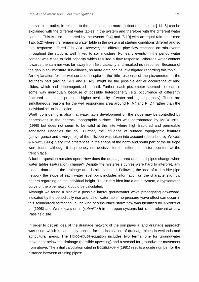
Results and discussion: Field investigations 59
the soil pipe outlet. In relation to the questions the more distinct response at [-14;-8] can be
explained with the different water tables in the system and therefore with the different water
content. This is also supported by the events [0;4] and [8;10] with an equal rain input (see
Tab. 5.2) where the remaining water table in the system at starting conditions differed and so
total response differed (Fig. A3). However, the different pipe flow response on rain events
throughout the study is well linked to soil moisture. For early events in the period water
content was close to field capacity which resulted a flow response. Whereas water content
towards the summer was far away from field capacity and resulted no response. Because of
the gap in soil moisture surveillance, no more data can be investigated regarding this topic.
An explanation for the wet surface, in spite of the little response of the piezometers in the
southern part (around SP1 and P_A2), might be the possible earlier occurrence of land
slides, which had dehomogenized the soil. Further, each piezometer seemed to react, in
some way individually because of possible heterogeneity (e.g. occurrence of differently
fractured sandstone, proposed higher availability of water and higher porosity). These are
simultaneous reasons for the well responding area around P_A7 and P_C7 rather than the
individual setup installation.
Worth considering is also that water table development on the slope may be controlled by
depressions in the bedrock topographic surface. This was corroborated by MCDONNELL
(1998) but does not seem to be valid at this site where high fractured and permeable
sandstone underlies the soil. Further, the influence of surface topographic features
(convergence and divergence) of the hillslope was taken into account (described by WOODS
& ROWE, 1996). Very little differences in the shape of the north and south part of the hillslope
were found, although it is probably not decisive for the different moisture content at the
trench face.
A further question remains open: How does the drainage area of the soil pipes change when
water tables (saturation) change? Despite the hysteresis curves were hard to interpret, any
hidden data about the drainage area is still expected. Following the idea of a dendrite pipe
network the slope of each water level point includes information on the characteristic flow
patters regarding on the individual height. To join this idea into a drain system, a hypsometric
curve of the pipe network could be calculated.
Although we found a hint of a possible lateral groundwater wave propagating downward,
indicated by the periodically rise and fall of water table, no pressure wave effect can occur in
this soil/bedrock formation. Such kind of subsurface storm flow was identified by TORRES et
al. (1998) and WENNINGER et al. (submitted) in non-open systems but is not relevant at Low
Pass field site.
In order to get an idea of the drainage network of the soil pipes a land drainage approach
was used, which is commonly applied for the installation of drainage pipes in wetlands and
agricultural areas. The HOOGHOUDT-equation includes two terms, one for groundwater
movement below the drainage (possible upwelling) and a second for groundwater movement
from above. The initial calculation cited in EGGELSMANN (1981) results a guide number for the
distance between draining pipes:

Results and discussion: Field investigations 60
⋅⋅+
⋅⋅⋅=
shK
shdKa
21
22 44
(E. 5.5.4)
where: a = distance between draining pipes [m]
K1 = hydraulic conductivity above pipe level [m/d]
K2 = hydraulic conductivity below pipe level [m/d]
d = factor, relaying on the depth of soil horizon below soil pipe [-]
h = height of ground water table above pipe level [m]
s = maximal outflow to be drained by the system, pipe flow [m/d]
For this this approach the first term (contribution from below) was neglected. Including the
hydraulic conductivity determined by the slug test, the maximal specific pipeflow (determined
by max. DCA) of different events, and the piezometer levels it was possible to get a rough
assumption on the distance between draining pipes. This value is based on parallel installed
drainage pipes but can be related to the drainage network of the natural soil pipes.
Calculations were performed for peak IDs 4 + 5 and 6, for different assumed hydraulic
conductivities, for different elongation of water tables, and for different DCAs. The results
obtained in Tab. A5 for the distance between draining pipes varied around 1 m. Although it is
unlikely to come across parallel pipes the area of interpretation was extended towards the
shape of the network. This is finally interpreted in the way that the soil pipes network is well
connected and out branching does occur within the scale of 1 m. If this knowledge is
transferred to the field site, there is a hint on the occurrence of many soil pipe draining
structures along the width of the investigated hillslope (30 m).
5.6 Discharge at weir
The weir measured the initial stream running out of the proposed well at the lower hillslope.
Obvious graph characteristic are the gaps of the series. Reasons here fore were the branch
jams in the notch, which provided error data. This was likely to occur in a forested
environment even under high maintenance.
As the weir was installed later, the first available data capture the response on rainfall event
[0;4]. Peak discharge of the flume, 640 l/10 min, was about 6.5 times higher than the peak of
the soil pipes. The total flow amount for this event ID 6, according to the limitations in
Tab. A3 was 4110 m³. This was shown to be 26 times higher than soil pipe total event flow
volume. Because the determination of a drainage area was difficult, no specific discharge
was calculated for this peak event. The turquoise graph presented in Fig. 5.6a is
standardized based on the maximum peak of soil pipe discharge. This helps to make
comparisons between the response of soil pipe and weir discharge.

Results and discussion: Field investigations 61
The data presented in Fig. 5.6a also show a second peak for weir flow around day 24.
Although these data are discontinuous, the general response according to the rainfall input is
more strongly pronounced than the soil pipes hydrograph during these dry conditions of the
system.
-10 0 10 20 30 40 No of days, relative to tracer application on April, 2
0
50
100
150
200
250
300
350
400
450
500
550
600
650
700
Dis
char
ge [
l / 1
0min
]
50
45
40
35
30
25
20
15
10
5
0
Thro
ughf
all P
reci
ptat
ion
[mm
/ da
y]
-10 0 10 20 30 40
ThroughfallQ weirQ soil pipesQ weir standardized
Fig. 5.6a: Discharge of weir, soil pipes, and standardized weir flow. Finally the temporal delay between the soil pipe hydrograph and the hillslope hydrograph
(weir) are illustrated for the event ID 6. The peak of the weir hydrograph was delayed by
7 hours compared to the pipe flow peak (Fig. 5.6b).

Results and discussion: Field investigations 62
-1 0 1 2 3 4 5 6 7 8 9 10 No of days, relative to tracer application on April, 2
0
50
100
150
200
250
300
350
400
450
500
550
600
650
700D
isch
arge
[ l /
10m
in]
109876543210
Thro
ughf
all P
reci
ptat
ion
[mm
/ da
y]
-1 0 1 2 3 4 5 6 7 8 9 10
ThroughfallQ weirQ soil pipes
Fig. 5.6b: Time shift of pipe flow and weir hydrograph for event related to tracer
injection (peak ID 6).
Discussion of weir flow
Based on the portions of pipe flow and stream flow for event ID 6, the percentage of
streamflow generated by pipeflow of the studied soil pipes is 3%. This result is consistent
with the observations of TURTON et al. (1992), where subsurface flow at a plot scale
contributes little to quickflow. Nevertheless, for this view it is important to outline that there
are probably more subsurface flow paths, like other soil pipes, which could not be included in
this comparison. Concerning these different drainage areas the percentage might be higher
and should be treated with scepticism.
Furthermore, the forest road has important influence. Here, a great deal of literature focuses
on these runoff generation processes summarised by LUCE (2002). The behaviour and
dependency of cutslopes interception and its contributions is still not clear. The subsurface
portion of flow contribution is strongly connected to a seasonally high water table.
Observations from the Oregon Coast Range show that some roads intercept subsurface flow
even when the water table is below the road (LUCE, 2002). Former studies at the Low Pass
field site addressed this focus on the road section. However, the influence of the forest road
with its extended contribution area and the amount of the already measured uphill pipeflow
has an effect on the interpretation of the weir hydrograph. E.g. take into account that the
already measured tipping bucket outflow was served into the catchment of the weir.

Results and discussion: Field investigations 63
Looking beyond the end of the visible initial stream, where old trees hide the water at some
stages, the true origin of the stream would be expected. This might be a spring with even
similar characteristics to the soil pipes, and would lead to some discussion about the
difference and the terminology in general. This may be called confluence for the catchment
area and raises questions about the water origin at this opening. The much lower altitude
suggests a strong domination of groundwater rather than any interflow (see definition of
“spring”). To what extent this water differs from the soil pipe water could not be investigated
in this study. In conclusion weir discharge presumably includes a majority of groundwater.
Further possible interpretation and general conclusions are demonstrated later in Fig. 5.8.
5.7 Results tracer experiments
5.7.1 Amio G Acid Lysimeter To begin, it is important to note that the measurements represent integrated data, as the
suction was kept for one to three days. The upper suction lysimeter (L_U) reported basically
the movement of the tracer front through the soil. This is presented in Fig. 5.7.1 for soil
depths of 30, 50, and 70 cm. Data smaller than 30 ppb are treated as fuzzy data, as
background concentration in the humus layer is able to achieve such values.
The first detection of tracer in the 30 cm suction cup occurred one day after the application.
So the tracer went rapidly through the humus layer outlined in section 3.3. In the following
days up to day 9 the full tracer breakthrough took place in the 30 cm depth. The thinned out
concentration towards the end indicate a tailing of the curve.
The first arrived tracer 20 cm lower (at 50 cm total soil depth) is proposed to be at day 5 with
76 ppb. The following dry period did not cause much tracer movement. Not even a tailing of
the first peak is visible. The second rise up on day 21 is explained by rainfall of 28 mm on
that day which mobilized further tracer. Unfortunately further data could not be provided as
the water content was too small to allow any sampling.
At a the soil depth of 70 cm no tracer occurred. The reason therefor might be the not yet
detected entire breakthrough at a 50 cm depth.

Results and discussion: Field investigations 64
0 1 2 3 4 5 6 7 8 9 10 11 12 13 14 15 16 17 18 19 20 21 22 23 24 25No. of days after tracer application on April, 2
0
10
20
30
40
50
60
70
80C
once
ntra
tion
Am
ino-
G A
cid
[ppb
]
0
10
20
30
40
50
60
70
80
0 1 2 3 4 5 6 7 8 9 10 11 12 13 14 15 16 17 18 19 20 21 22 23 24 25
Depth: 30 cmDepth: 50 cmDepth: 70 cm
Fig. 5.7.1: Concentration of Amino G Acid at suction lysimeter below the line source tracer application.
Piezometer The samples sucked out of the piezometer are rare, because in a lot cases not enough water
was in there to provide the required sample minimum (see section 5.5). No significant tracer
concentration was found within the grid capturing likely pathways. Background
concentrations here were around 10 ppb, probably caused by high sediment content or
interactions with the bitumen or PVC shavings (might had been some mistaken leftovers).
Soil pipes and flow proportional samples at tipping buckets The hand samples at the three different soil pipes endings did not show an Amino G Acid
breakthrough. The detected concentrations were within the background or close to the
detection limit and are classified as no tracer breakthrough.
The flow proportional sampler at the tipping buckets offered continuous surveillance for a
tracer breakthrough. For the period investigated no breakthrough curve was detected.
Weir The hand samples at the weir resulted in a single peak (digital time 4.5) of 43 ppb. Beside
that no other samples contained Amino G Acid. Therefor an error is supposed for the outlier.
Summarizing this study has no evidence of any tracer arrival at the lowest point of sampling
and presumes overall confluence.
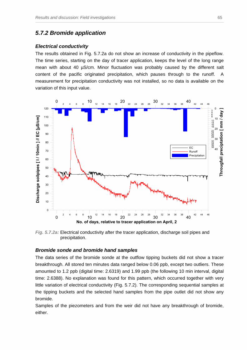
Results and discussion: Field investigations 65
5.7.2 Bromide application Electrical conductivity The results obtained in Fig. 5.7.2a do not show an increase of conductivity in the pipeflow.
The time series, starting on the day of tracer application, keeps the level of the long range
mean with about 40 µS/cm. Minor fluctuation was probably caused by the different salt
content of the pacific originated precipitation, which pauses through to the runoff. A
measurement for precipitation conductivity was not installed, so no data is available on the
variation of this input value.
0 10 20 30 402 4 6 8 12 14 16 18 22 24 26 28 32 34 36 38 42 44 46
No. of days, relative to tracer application on April, 2
0
10
20
30
40
50
60
70
80
90
100
110
120
Dis
char
ge s
oilp
ipes
[ l /
10m
in ]
// EC
[µS/
cm]
40
30
20
10
0
38363432
28262422
18161412
8642
Thro
ugfa
ll pr
ecip
tatio
n [ m
m /
day
]
0 10 20 30 402 4 6 8 12 14 16 18 22 24 26 28 32 34 36 38 42 44 46
ECRunoffPrecipitation
Fig. 5.7.2a: Electrical conductivity after the tracer application, discharge soil pipes and precipitation.
Bromide sonde and bromide hand samples The data series of the bromide sonde at the outflow tipping buckets did not show a tracer
breakthrough. All stored ten minutes data ranged below 0.06 ppb, except two outliers. These
amounted to 1.2 ppb (digital time: 2.6319) and 1.99 ppb (the following 10 min interval, digital
time: 2.6388). No explanation was found for this pattern, which occurred together with very
little variation of electrical conductivity (Fig. 5.7.2). The corresponding sequential samples at
the tipping buckets and the selected hand samples from the pipe outlet did not show any
bromide.
Samples of the piezometers and from the weir did not have any breakthrough of bromide,
either.
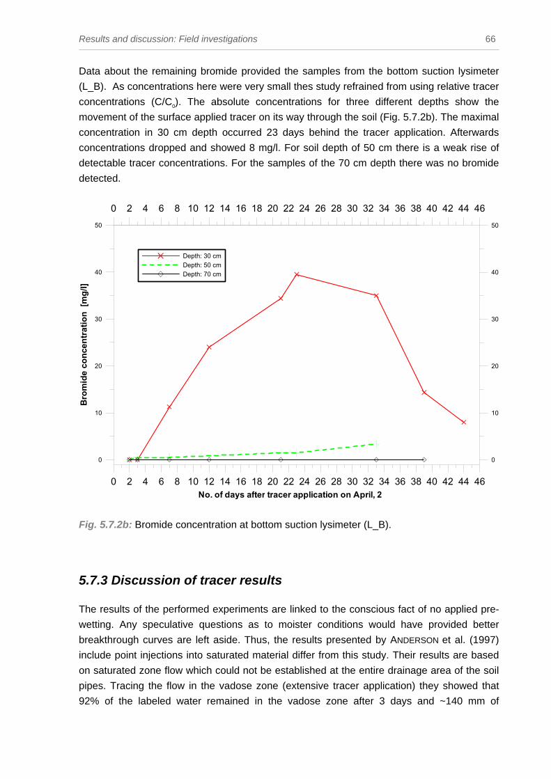
Results and discussion: Field investigations 66
Data about the remaining bromide provided the samples from the bottom suction lysimeter
(L_B). As concentrations here were very small thes study refrained from using relative tracer
concentrations (C/C0). The absolute concentrations for three different depths show the
movement of the surface applied tracer on its way through the soil (Fig. 5.7.2b). The maximal
concentration in 30 cm depth occurred 23 days behind the tracer application. Afterwards
concentrations dropped and showed 8 mg/l. For soil depth of 50 cm there is a weak rise of
detectable tracer concentrations. For the samples of the 70 cm depth there was no bromide
detected.
0 2 4 6 8 10 12 14 16 18 20 22 24 26 28 30 32 34 36 38 40 42 44 46No. of days after tracer application on April, 2
0
10
20
30
40
50
Bro
mid
e co
ncen
trat
ion
[mg/
l]
0
10
20
30
40
50
0 2 4 6 8 10 12 14 16 18 20 22 24 26 28 30 32 34 36 38 40 42 44 46
Depth: 30 cmDepth: 50 cmDepth: 70 cm
Fig. 5.7.2b: Bromide concentration at bottom suction lysimeter (L_B).
5.7.3 Discussion of tracer results The results of the performed experiments are linked to the conscious fact of no applied pre-
wetting. Any speculative questions as to moister conditions would have provided better
breakthrough curves are left aside. Thus, the results presented by ANDERSON et al. (1997)
include point injections into saturated material differ from this study. Their results are based
on saturated zone flow which could not be established at the entire drainage area of the soil
pipes. Tracing the flow in the vadose zone (extensive tracer application) they showed that
92% of the labeled water remained in the vadose zone after 3 days and ~140 mm of

Results and discussion: Field investigations 67
sprinkling. However, their lysimeter observations with about the same installation and
conditions (depth 0.87 m and 0.21 m) fit well to these ones. For an interpretation of the suction cup data problems arised from the dissolved organic
carbon, as in particular concentrations ranged low. Beside this background issue note that
solute sampling is likely to miss bypass flow (FLURY et al., 1994). As bypass flow was
proposed in this kind of soil (see above), it may also be valid that Amino G Acid (applied at
20 cm distances) used a macropore system to bypass the sampling cup. But as the data of
the bromide movement showed very similar results a remainder of both tracers in the upper
50 cm of the soil is summarized.
Reasons for the absence of tracer at the soil pipe outlets and at the weir The transit times of the tracer up to the soil pipe did exceed the investigation period and
remained in the system.
A major reason here is the reduced precipitation (113 mm) falling after April, 2 why further
events did not mobilize the tracer enough. For the line source application and the extensive
application it is shown that the tracer did hardly reach a soil depth of 70 cm. So the drained
soil matrix had too little conductivity to enable faster tracer movement. On the evidence it is
likely that most tracer was held up or stuck in the micropore system of the unsaturated zone.
The status of saturated conditions with higher velocities could not be obtained. This was
particularly difficult because piezometer data showed the unsaturated conditions during the
whole period in the upper 70 cm soil depth (see section 5.5). Similar results where tracer
‘stranded’ in the unsaturated zone are apparently described by NYBERG et al. (1999) and
WILSON et al. (1993). But within the logic of this interpretation a further process is not able to
be described: How does it come that a little peak of discharge occurred (ID 6) and although a
quick piezometer response after storm events indicates a fast acting water table
establishment from above whereas there is no evidence of tracer movement?
Another further consulted interpretation focuses on the tracer input mass being too small.
Two aspects appear to be relevant: Unexpected high sorption and dilution. Both phenomena
are already detected for the restrictively applied line tracer in 70 cm depth (Fig. 5.7.1). And
on its further path, even if little tracer reached saturated conditions a very strong dilution
made a determination impossible. This effect also played out particularly at the weir, where a
high portion of ground water contributed to runoff. Further, regarding the soil pipes, the
maximal dynamic contributing area (section 5.4.1) outlined that a high solution is likely.
Instead of a wider distribution of the area sprinkled with bromide (towards the higher gradient
in topography in the south) a higher tracer input mass might be the better approach.
Concluding, the assumed contributed discharge for the tracer input mass calculation was too
small.

Results and discussion: Field investigations 68
5.8 Conclusions of field investigations The characteristic in Coast Range rainfall intensities distribution, with outstanding peaks
throughout a low intensity (Fig. 5.2c), is assumed to be a trigger mechanism for runoff
generation. Whether the pipe response is linked to higher intensities could not be
investigated comprehensively.
The results of pipeflow imply that there was a component of rapid contribution from rising
water tables as a consequence of a supposed dendritic network upslope with its spatial
increase of drainage network. Taking the obvious response (rise of water table) into account,
it might be questioned, why no tracer reached the saturated conditions? The answers on this
topic about local groundwater recharge are discussed in two ways. First, regarding the water
content of the soil, much water is needed to achieve field capacity. And even under
macropore conditions preferential flow is inhibited by the unsaturated conditions. Thus, the
rise of water table is caused by ‘old’ water rather than by ‘new’ water, which would have
contained tracer concentration. Second, there has been no focus, whether interflow from the
top hillslope area is able to cause a water table rise. However, there is a second component
of groundwater, which is responsible for the long-term delivery. This is based on the
ephemeral pattern of pipe flow and its summer drought. The impact of groundwater from
below on pipe flow is e.g. supported by the position and horizontal alignment of the pipe
outlets; and the temporal start up of SP2 and SP3 probably is created by a possible
threshold mechanism. Piezometer data showed that the water table in the hillslope was
highly variable in both magnitude and timing. And even neighbouring piezometers showed
unexpected differences. But temporary water tables in the hillslope occurred up to 60 cm
below surface topography and are well linked to the pipeflow hydrograph. Orientating on the
question about the affection of topographic convergence on subsurface flow and water
tables, the findings provide evidence for higher water tables levels and oscillation in the less
convergent, northern part of the hillslope.
This might also be explained by the shape of the dentritic network and the connection of
different areas to it. This hypothesis would explain the different piezometer response.
However, verification of this network shape is e.g. possible by a fibrescope examination on
morphologic triple-junction features (TERAJIMA et al., 2000). Nevertheless, an absence of this
drainage mechanism of the pipes would otherwise cause a saturation of soil with occuring
interflow components at the trench section. Fig. 5.8 gives an outline on ideas about processes and conditions of flow. The proposed
water table shows an annual magnitude and therefore the drainage area of the pipe network
differs throughout the year. For the high water table levels during winter we see a water table
rise supported by winter frosts with open cracks and strong stability of soil aggregates. A
similar context is shown in the results of TSUKAMOTO et al. (1982) who reported that pipe flow
did not begin until groundwater saturation reached the pipe level.

Results and discussion: Field investigations 69
Fig. 5.8: Assumed processes and conditions along transect of the hillslope.
The role of bedrock is still not clear. However, there is a certain interaction between key-
mechanism water table and the fractured underlying bedrock formation, with leaky
properties. Further, there was found no hint about a connection of the water table in the
slope and other indication of ground water.
The hydraulic connection of lateral flow in the macroporous soil and the horizontal dominated
soil pipes (likely to be seasonal groundwater table) is still unsure, as the outcome of the
tracer experiments provided no successful information. The pattern that flow begins only
when soil is almost saturated is a well known fact for macropore flow (e.g. JOERIN et al.,
2002) was supported by selected data presented above.
The question how old the dominating pipe flow is (dominated by ‘old’ groundwater or rather
event water) is not clarified satisfactorily with this tracer study. Mean turnover times of
recessions could also not help to solve this problem although residence time (tracer
experiment) does outstrip mean turnover times (recession analysis) by far.

Results and discussion: Field investigations 70
Estimated reasons for the unsuccessful tracer experiment are the reduced precipitation input
and the dry conditions in the unsaturated zone. For the objective of the study the hillslope is
still to be treated as a ‘black box’. A proposed outlook may be the excavating of tracer for
determination of already travelled distance or, alternatively, to wait for the next wet season.
The results presented are a snapshot of conditions as soil pipes develop and change, visible
in varying sediment discharge within years (UCHIDA et al., 1999). The reason here is the non-
DARCY flow in a soil pipes with its acceleration and erosion. Moreover,
WILSON & SMART (1984) predict that soil pipes modified their hydraulic properties to produce
an efficient drainage network.

Results and discussion: Hillslope table 71
6 Results and discussion: Hillslope table The availability of sophisticated hydrological models has greatly improved hydrologists ability
to perform complex hydrological analyses. Models make it feasible to evaluate the impact of
soil pipes on stream flow generation. This chapter follows the question of how an artificial
simulation of the conditions of a field site actually operates in practice.
The results presented are the starting point for further studies, which will include artificially
implemented soil pipe structures (see section 6.8). This physical modelling approach might
help to gain knowledge about the connection of lateral and transverse macropores at the
Low Pass field site and in general.
6.1 Short overall description of the experimental run Preliminary initial experiments helped to assess the response and conditions of the table.
The very first stages of the sprinkling experiment were performed at a slope of 5%, and
resulted in a strong occurrence of Hortonian Overland Flow. An additional textile layer was
placed on top of the soil, with the intention of improving the infiltration capacity by the
enhanced roughness, which would hinder landed drops from transverse flow. But this did not
reduce surface runoff either.
The final run was included at a slope of 25% and included the three days May, 19 to May,
22. In what follows, time is expressed as digital time.
6.2 Sprinkling
The sprinkling intervals were chosen small enough in order to prevent Hortonian Overland
Flow and frequently enough to ensure steady state conditions at the outflow. A unit consisted
of 5 minutes’ irrigation, with an average of 2.338 mm or 18.23 l sprinkling. It was followed by
10 min draining. For a simulation a combination of looping units was applied. This was in
order to catch up with the idea of mostly low rainfall quantities with high peaks included. After
about five to six loops, there was a longer drainage period, which was also varied in its
length. The schedule of irrigation runs and drainage stages for the whole experiment is
reported in appendix B1.
At the end of the experiments a series of 10 min sprinkling events was performed with a
10 min break in between. The reason for this was a final mobilisation of any remaining tracer
in the system. As a result of the extended sprinkling interval the occurrence of little
HORTONian Overland Flow was taken into account.
The temporal distribution of sprinkling (on / off application) over the experimental period is
presented in Fig. 6.2.
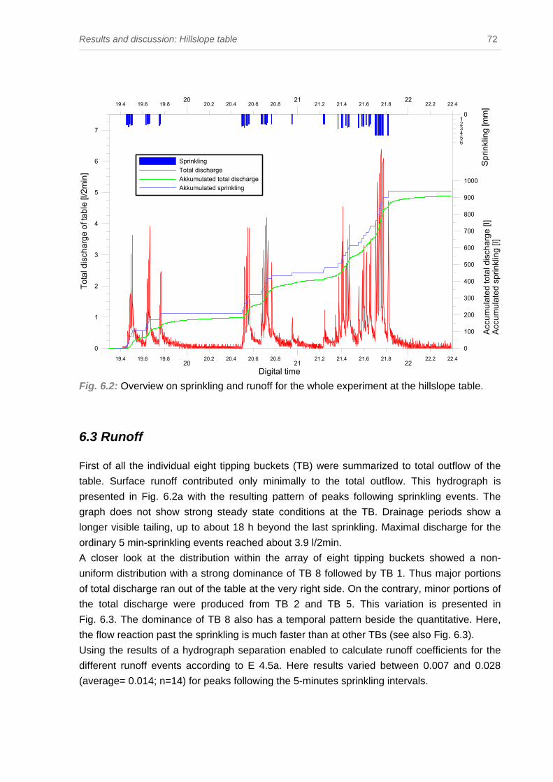
Results and discussion: Hillslope table 72
20 21 2219.4 19.6 19.8 20.2 20.4 20.6 20.8 21.2 21.4 21.6 21.8 22.2 22.4
Digital time
0
1
2
3
4
5
6
7
Tota
l dis
char
ge o
f tab
le [l
/2m
in]
0
654321
Spr
inkl
ing
[mm
]
20 21 2219.4 19.6 19.8 20.2 20.4 20.6 20.8 21.2 21.4 21.6 21.8 22.2 22.4
SprinklingTotal dischargeAkkumulated total dischargeAkkumulated sprinkling
0
100
200
300
400
500
600
700
800
900
1000
Acc
umul
ated
tota
l dis
char
ge [l
]A
ccum
ulat
ed s
p rin
klin
g [l]
Fig. 6.2: Overview on sprinkling and runoff for the whole experiment at the hillslope table.
6.3 Runoff First of all the individual eight tipping buckets (TB) were summarized to total outflow of the
table. Surface runoff contributed only minimally to the total outflow. This hydrograph is
presented in Fig. 6.2a with the resulting pattern of peaks following sprinkling events. The
graph does not show strong steady state conditions at the TB. Drainage periods show a
longer visible tailing, up to about 18 h beyond the last sprinkling. Maximal discharge for the
ordinary 5 min-sprinkling events reached about 3.9 l/2min.
A closer look at the distribution within the array of eight tipping buckets showed a non-
uniform distribution with a strong dominance of TB 8 followed by TB 1. Thus major portions
of total discharge ran out of the table at the very right side. On the contrary, minor portions of
the total discharge were produced from TB 2 and TB 5. This variation is presented in
Fig. 6.3. The dominance of TB 8 also has a temporal pattern beside the quantitative. Here,
the flow reaction past the sprinkling is much faster than at other TBs (see also Fig. 6.3).
Using the results of a hydrograph separation enabled to calculate runoff coefficients for the
different runoff events according to E 4.5a. Here results varied between 0.007 and 0.028
(average= 0.014; n=14) for peaks following the 5-minutes sprinkling intervals.

Results and discussion: Hillslope table 73
Timing
The time shift (according to section 4.5) between runoff peak and the 5-minutes sprinkling
events ranged between 2.5 and 4.5 min, average was 3.46 min (n=36). No significant relation
with soil moisture data was found.
20 21 2219.4 19.6 19.8 20.2 20.4 20.6 20.8 21.2 21.4 21.6 21.8 22.2 22.4
Digital time
0
100
200
300
400
500
600
700
800
900
Acc
umul
ated
tota
l dis
char
ge [l
]
0
654321
Spr
inkl
ing
[mm
]
20 21 2219.4 19.6 19.8 20.2 20.4 20.6 20.8 21.2 21.4 21.6 21.8 22.2 22.4
SprinklingTotal TBTB 8TB 7TB 6TB 5TB 4TB 3TB 2TB 1
Fig. 6.3: Variability of accumulated discharge at different tipping buckets and sprinkling intervals. Discussion of Runoff
The non-uniform distribution of discharge at the TBs was not expected. In view of the
homogenous rainfall distribution (mentioned earlier) and the horizontal alignment of the table
ground, either a proportionately greater runoff might be expected at TB 3 to TB 5 (all in the
middle) or else an even runoff for all TBs. For an explanation of the actual result importance
has to be attached to soil properties. The irregularity is obviously caused by the soil filling,
although this was done with maximum precision.
The occurrence of surface runoff is best explained by there is a missing vegetation layer and
A-horizon. These findings contrast to other sprinkling studies on a comparable soil, with
much greater slope angles (43°) and durations of 10 to 30 min where no surface runoff

Results and discussion: Hillslope table 74
occurred (TORRES et al., 1998). Both experiments highlighted that soil-water content does not
influence the generation of HORTONian Overland Flow.
6.4 Water balance
For the overall run, which included three days of investigation, a total amount of 935.8 l of
rain was applied to the table. The total runoff for the same period amounted to 910.6 l.
Therefore the water balance shows a gap of 25.2 l, which is water remaining in the soil and a
minimal portion of eventually evaporated water.
6.5 Soil moisture The soil moisture data of three differently located sensors are presented in Fig. 6.5. During
the experiment the volumetric water content of the soil ranged between about 25 and 35%.
The calculated mean drainable porosity amounts to 8%. Using a piston core device at digital
time 22.4 provided a soil water content of 0.61 g/cm³ for the probe B. The linkage of
volumetric water content (output logger) and absolute water content resulted in a water
content of 0.87 g/cm³ for saturated conditions of probe B.
The graph of the deeper probes A and C shows that the system was saturated for most of
the time. Within the overnight drainage periods water volume reduced but still did not reach a
limit. Contrary sonde B shows this very well. Here, four centimetres below soil surface, the
rapid drainage even in short sprinkling breaks dominated.

Results and discussion: Hillslope table 75
20 21 2219.4 19.6 19.8 20.2 20.4 20.6 20.8 21.2 21.4 21.6 21.8 22.2 22.4
Digital time
0
0.05
0.1
0.15
0.2
0.25
0.3
0.35
0.4V
olum
etric
wat
er c
onte
nt0
654321
Spr
inkl
ing
[mm
]
20 21 2219.4 19.6 19.8 20.2 20.4 20.6 20.8 21.2 21.4 21.6 21.8 22.2 22.4
Sonde A: x=40, y=110, z=-9 Sonde B: x=118, y=120, z=-4 Sonde C: x=158, y=110, z=-8 Sprinkling
Fig. 6.5: Soil moisture at three different locations at the table for the period of experiment. Discussion of soil moisture
Constant soil moisture content is typical for steady state irrigation. Although this was not
obtained perfectly, approximate ‘steady state’ conditions were achieved. These results are
consistent with FEYEN et al. (1999) for example, who sprinkled a muck plot
6.6 Water table and water volume To visualize the water table levels a spatial distribution was chosen. The data of the mini
piezometer was interpolated by the Kriging-method. Length numbers where y is ∈ [0, 78]
were excluded from interpolation. Because of that, there was an illustration much closer to
reality than the one with the border issue zero instead. This would result in a declining water
table towards y= 0 which is contrary to the natural conditions. Because the table was actually
sloping, a small extended water table was ‘backed up’ from the outlet and rose
disproportionately in this not interpolated zone. A complete saturation of the soil - with water
level with the surface of the soil - was observed in this area rarely (especially at the 10 min
sprinkling intervals).
The spatial interpolation was prepared for the first day of experiments on selected time steps
(Fig. 6.6a). Generally, the water table moved slower than the runoff response. The water
table was established from lower regions, where water was backed up on the sloping table.
This process is more or less uniformly and reached up to a water level height of 13 cm. After

Results and discussion: Hillslope table 76
the rise of the table around digital time 19.5 the maximum in both height and extension was
obtained. The subsequent decline towards the next day happened slowly, in particular
between digital time 20 and 20.45. This underlined the characteristics of the system. The
decline of the water table during the recession period, starting at 19.82, was not uniform and
showed priority at the left hand side of the table (TB 1).
0 20 40 60 80 100 120 140 160 1800
20
40
60
80
100
120
140
160
180
200
220
240
260
280
300
320
340
360
380
0 20 40 60 80 100 120 140 160 1800
20
40
60
80
100
120
140
160
180
200
220
240
260
280
300
320
340
360
380
11.20 h (19.472)
11.30 h (19.479)

Results and discussion: Hillslope table 77
0 20 40 60 80 100 120 140 160 1800
20
40
60
80
100
120
140
160
180
200
220
240
260
280
300
320
340
360
380
0 20 40 60 80 100 120 140 160 1800
20
40
60
80
100
120
140
160
180
200
220
240
260
280
300
320
340
360
380
12.00 h (19.5)
12.26 h (19.518)
Fig. 6.6a: Height of water table [mm] at different time steps. See legend on right for details. Dimension of table [cm].
0 20 40 60 80 100 120 140 160 1800
20
40
60
80
100
120
140
160
180
200
220
240
260
280
300
320
340
360
380
0 20 40 60 80 100 120 140 160 1800
20
40
60
80
100
120
140
160
180
200
220
240
260
280
300
320
340
360
380
13.10 h (19.549) 15.18 h (19.638)
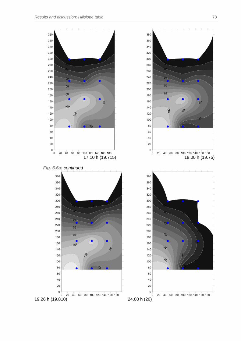
Results and discussion: Hillslope table 78
0 20 40 60 80 100 120 140 160 1800
20
40
60
80
100
120
140
160
180
200
220
240
260
280
300
320
340
360
380
0 20 40 60 80 100 120 140 160 1800
20
40
60
80
100
120
140
160
180
200
220
240
260
280
300
320
340
360
380
17.10 h (19.715) 18.00 h (19.75)
Fig. 6.6a: continued
0 20 40 60 80 100 120 140 160 1800
20
40
60
80
100
120
140
160
180
200
220
240
260
280
300
320
340
360
380
0 20 40 60 80 100 120 140 160 1800
20
40
60
80
100
120
140
160
180
200
220
240
260
280
300
320
340
360
380
19.26 h (19.810) 24.00 h (20)

Results and discussion: Hillslope table 79
0 20 40 60 80 100 120 140 160 1800
20
40
60
80
100
120
140
160
180
200
220
240
260
280
300
320
340
360
380
0 20 40 60 80 100 120 140 160 1800
20
40
60
80
100
120
140
160
180
200
220
240
260
280
300
320
340
360
380
next day 7.00 h (20.292) next day 11.00 h (20.458) Fig. 6.6a: continued Out of these interpolated spatial water table data the total water volume in the table was
calculated based on the measurements of absolute water content under saturated
conditions. The data of sonde B was extrapolated to the overall soil. However, this offered
an estimation of water volume in the system and is provided in Fig. 6.6b for a initial run of
experiments. During saturation conditions the maximal water volume remaining in the system
was about 400 l. The recession at the end was slow and went down to an amount of 50 l.

Results and discussion: Hillslope table 80
19.4 19.6 19.8 20 20.2 20.419.45 19.5 19.55 19.65 19.7 19.75 19.85 19.9 19.95 20.05 20.1 20.15 20.25 20.3 20.35
Digital time
0
1
2
3
4
5To
tal d
isch
arge
tabl
e [l
/ 2m
in]
4644424038363432302826242220181614121086420
Spr
inkl
ing
[mm
] //
Wat
er v
olum
e [d
ecal
iter]
19.4 19.6 19.8 20 20.2 20.419.45 19.5 19.55 19.65 19.7 19.75 19.85 19.9 19.95 20.05 20.1 20.15 20.25 20.3 20.35
3.12
15.8
30.9
36.5
40.4
36.3
29.2
22.4
28.5
41
35.1
28.4
35.8
31.8
28.8
18.8
12.8
6.535
SprinklingTotal dischargeWater volume
Fig. 6.6b: Sprinkling, runoff and water volume for the first interval of the experiments.
The time shift between precipitation and peak of water volume (refer section 4.5) was
calculated to 74, 42, and 76 min (in chronological order).
Discussion of water table and water volume
The symmetry of the water table movement is relevant for an assessment of the soil filling.
The shown data with a left dominated table recession is contrary to the runoff distribution at
the TBs. No explanation was found for this pattern. A remark highlights the assumptions of
the interpolation method, which blur the pattern. Finally it is concluded that once again the
properties of the artificial filling trigger this pattern and are a major factor.
For the discussion of water balance calculation (section 6.4) additional data can be included.
A comparison of the gap in the measured water balance (25.2 l) and the estimated water
volume in the system (50 l) provides somehow an explanation. Bridging the gap in the
balance is not possible with the inexactness contained by the interpolation method. However,
the results showed that the estimated numbers fit roughly.
6.7 Tracer For the interpretation of the Amino G Acid line source application and the Brilliant Blue line
source the amount of sprinkling upslope the line was of major interest, rather than the total

Results and discussion: Hillslope table 81
amount of sprinkling for the table. This input resulted in lateral flow which was able to
mobilize the tracer, plus of course the little amount of sprinkling which fell directly on the line.
The line source of Amino G Acid was set at y= 285 cm and Brilliant Blue FF was set at y=
290 cm. The distribution of sprinkling was already shown in Fig. 3.2.5b and pointed out the
decrease of precipitation in this area. A calculation based on an interpolated Kriging
approach got an integrated total sprinkling amount above y= 280 cm of 7.7 mm/hr. This is
valid until digital time 21.3722, when a nozzle modification extended the area of intense
sprinkling by about 15 cm towards upslope. The increased sprinkling input above the line
source, which was able to carry the dye, was then interpolated to 13 mm/hr.
Generally tracer mobilisation is controlled by the non steady state conditions. For the
5-minutes sprinkling events no overlapping of flow paths due to occuring HORTONian
overland flow was asumed.
6.7.1 Amino G Acid line source
For the entire experimental run the line source remained in an unsaturated environment; this
was shown in section 6.6.
Results
The results of the Amino G line source experiment need special treatment as they are not
clear and are hard to interpret. In order to clarify the pattern, Amino G concentrations below
20 ppb were treated as high background concentrations (MCGUIRE, personal
communications; SMART & LAIDLAW, 1977). This data of no tracer breakthrough record is
caused by high dissolved organic carbon (DOC) concentrations.
Sampling at the mini piezometers in the middle of the table did not result in any positive
tracer record! Values here ranged within the background level.
A detailed view of the results of the tracer breakthrough at the final TBs is described now. As
the corresponding runoff differed strongly (s. above) tracer breakthrough also varied between
the individual TBs. The first one described is TB 8, which is singled out because of its major
portion within total discharge. Tracer concentrations showed a very unusual pattern which is
not comparable with a typical tracer breakthrough curve. Despite background concentration
a clear tracer breakthrough is not detectable in Fig. 6.7.1a.

Results and discussion: Hillslope table 82
20 21 2219.4 19.6 19.8 20.2 20.4 20.6 20.8 21.2 21.4 21.6 21.8 22.2 22.4
Digital time
0
100
200
300
400
500
600
700
800
900
1000D
isch
arge
at T
B 8
[m
l/2 m
in]
60
50
40
30
20
10
0
6462
58565452
48464442
38363432
28262422
18161412
8642
Spr
inkl
ing
[mm
] // A
min
o-G
con
cent
ratio
n at
TB
8 [µ
g/l]
20 21 2219.4 19.6 19.8 20.2 20.4 20.6 20.8 21.2 21.4 21.6 21.8 22.2 22.4
SprinklingTracer conc.Discharge
Fig. 6.7.1a: Amino G concentration and discharge at TB 8.
Fig 6.7.1b is a different presentation of the same data including accumulated discharge (Fig.
6.7.1b). A third version includes a flow-proportional illustration of the same data (Fig. 6.7.1c).
The fact of high variations on Amino G concentrations is still obvious and this presents a
difficult situation for the interpretation of the data.

Results and discussion: Hillslope table 83
20 21 2219.4 19.6 19.8 20.2 20.4 20.6 20.8 21.2 21.4 21.6 21.8 22.2 22.4
Digital time
0
20
40
60
80
100
120
140
160
180
200
220
240
Acc
umul
ated
dis
char
ge a
t TB
8 [
l]
0
10
20
30
40
50
2468
12141618
22242628
32343638
42444648
52
Am
ino-
G c
once
ntra
tion
at T
B 8
[µg/
l]
20 21 2219.4 19.6 19.8 20.2 20.4 20.6 20.8 21.2 21.4 21.6 21.8 22.2 22.4
SprinklingAcc. dischargeTracer conc.
4
0
Spr
inkl
ing
[mm
]
Fig. 6.7.1b: Amino G concentration, accumulated discharge and sprinkling for TB 8.
0 10 20 30 40 50 60 70 80 90 100 110 120 130 140 150 160 170 180 190 200 210 220 230 240 250
Accumulated discharge at TB 8 [l]
0
10
20
30
40
50
60
70
2468
12141618
22242628
32343638
42444648
52545658
62646668
Am
ino
G c
once
ntra
tion
at T
B 8
[µg/
l]
Fig. 6.7.1c: Accumulated discharge and Amino G concentration at TB 8.

Results and discussion: Hillslope table 84
So far, data presentation is of TB 8, where most of the discharge occurred. The results of the
other TBs showed the same unclear pattern, and do not contain any significant information
on tracer breakthrough either (Fig. B1- B7).
Recovery rate
The calculation of a recovery rate is difficult to obtain as concentrations of point
measurements did not show a typical breakthrough. Thus there was no way of interpolating a
continuous graph which allowed the calculation of a tracer recovery rate.
6.7.2 Discussion of Amino G Acid line source Generally, these findings of minor, almost random peaks at the TBs instead of no or either a
proper tracer breakthrough are suspicious, not satisfactory and thus open for discussion.
Although the observed pulse of tracer fits with the idea of a water push caused by the
sprinkling intervals and a final remobilisation of the remaining tracer. Thus the pulses could
also be governed by the flow and its longitudinal dispersion. By the way a common result in
unsaturated zone tracer experiments (SCHUDEL et al., 2003).
But the combination of these results at the outflow plus the samples of the mini piezometers
support the theory of no tracer breakthrough during the run of experiment. Amino G Acid
remained in the soil close below the line application. This trapping of tracer was caused by
the minor hydrological conductivity of the soil.
A further possible error, photo decomposition of Amino G Acid is to be neglected, as the
exposure to sunlight was zero during the subsurface flow in the table and very little towards
the sampling. The samples themselves were stored in the dark until the determination.
6.7.3 Bromide General, preliminary remarks
The system investigated by the extensive bromide applications contains two domains, the
vertical flow through the soil and the lateral flow towards the tipping buckets. Viewing the
upper and lower area of the slope with regard to section 6.6 both processes are a
combination of saturated and unsaturated conditions.
In agreement with the Amino G acid analyses selected data of TB 1 + 8 are presented.
Results
The surveillance on bromide was performed by a continuous monitoring of EC and
discontinuous, flow proportional hand samples. The link between, and its regressions are
presented in Fig. B8 + B10. However they show weak significances (R² =0.12 and R² =0.49).
As the deviation between the series is also visible, the regression between EC and bromide
concentrations was calculated again just for the first day. This increased confidences for TB
1 to R² =0.73 (Fig. B9). Concluding the data basis at TB 1 for the first day might be best, as

Results and discussion: Hillslope table 85
hand samples and EC-data fit best, whereas for TB 8 both series do not fit together well (see
Fig. B11). Therefore, the analysis of breakthrough integrated selected data of TB 1. Further
as series was restricted to the non-continuous hand samples, why it was refrained from
calculating recovery.
Bromide breakthrough at the outflow of TB 1, relaying on the samples, is characterised by a
major peak at around digital time 19.503 with a few spiky peaks afterwards
(Fig. 6.7.3a). This was also obtained by the continuous electrical conductivity, where the first,
major breakthrough took place in accompany with the hand samples. However, peaks of
electrical conductivity followed sprinkling events. The discrepancy increases towards the
end, in particular from time 21.6 on, when sampling concentrations went to zero and
sprinkling response still caused higher conductivities.
20 21 2219.4 19.6 19.8 20.2 20.4 20.6 20.8 21.2 21.4 21.6 21.8 22.2 22.4
Digital time
0
20
40
60
80
100
120
140
160
180
200
220
240
260
Acc
umul
ated
dis
char
ge a
t TB
1 [l
]
0
10
20
30
40
50
60
70
80
90
100
Sprin
klin
g [m
m ]
Bro
mid
e co
ncen
trat
ion
at T
B1
[mg/
l]EC
[µS/
cm]
20 21 2219.4 19.6 19.8 20.2 20.4 20.6 20.8 21.2 21.4 21.6 21.8 22.2 22.4
SprinklingAccummulated QBromide concentration (samples)EC at TB1
Fig. 6.7.3a: Bromide concentrations, electrical conductivity, sprinkling intervals and accumulated discharge at TB 1.
6.7.4 Discussion of bromide The presented tracer data of EC and samples at TB 1 includes both, reliable data and data
where interpretation might be difficult. The first tracer breakthrough occurred when the dry
table system got saturated. As the first sprinkling intervals avoided surface runoff, runoff at
the TBs represents exclusively ‘interflow’ of the table. Further tracer peaks following indicate
the remobilisation of water. This is particularly obvious at the time 20.4 past overnight
drainage.

Results and discussion: Hillslope table 86
Interpretation of the peaks in EC after time 21 as well as in general should take the likely
change in EC of the sprinkling water into account. The water came from the public water
supply and was not monitored for the total period, but rare single data showed no significant
change of EC.
Important to remark is the fact that bromide is treated as a conservative tracer. For these
experiments no sorption processes are assumed. Further interpretations on this tracer input
might be possible using different modelling approaches (e.g. MALOSCZEWSKI & ZUBER, 1996).
6.7.5 Dye tracing with Brilliant Blue The additional information on the tracer movement from a dye tracing experiment was very
helpful. The line source of Brilliant Blue FF was set at y= 290 cm at the digital time 20.4. In
the following sixteen of the 5-minute sprinkle events (sum of 10.2 mm above line) were
applied. As so far no breakthrough occurred the area of sprinkling was extended (mentioned
above). After another three 5-minute intervals the first tracer breakthrough at the mini
piezometers occurred at P_C3 which is at y= 240 cm. This happened at digital time 21.42
almost 24 hours past the injection and what triggered it off was probably the extended spray
area with higher input rates above the line source.
During the ongoing experiments no other mini piezometer (neither P_C4 nor row B at y=
160 cm) nor any tipping bucket recorded dye. Even the last more intense 10-minutes
sprinkling intervals did not result in any new dye occurrence. But still the colour of P_C3
remained throughout indicating active flow paths from the line downwards.
The final excavation found dye along intersects from the injection down to y=190 cm, where
only a tiny trace of indication was found. For photographic capture of the dye tracer and the
soil Fig. 6.7.5b+c also provides colour scale (JOBO lab equipment). The pictures show the
decline in intensity towards y=265 cm. An overall mapping of the distance covered by the dye
is shown in Fig. 6.7.5a. The maximum distance the dye travelled within preferential pathways
was therefore 1 m.

Results and discussion: Hillslope table 87
0 20 40 60 80 100 120 140 160 1800
50
100
150
200
250
300
350
Fig. 6.7.5a: Line source of Magic blue at y=290 cm and dye movement down slope. Illustrated are selected slices of soil profiles from excavation. Note the fading of dye tracer.
Fig. 6.7.5b: Documentation of Brilliant Blue pathways at y=265 cm. The colour scale is made by JOBO lab equipment.
Fig. 6.7.5c: Documentation of Brilliant Blue pathways directly at the line application
(y= 290 cm).
Results and discussion: Hillslope table 88
6.7.6 Discussion of dye tracing with Brilliant Blue In the interpretation of the very limited movement of the Brilliant Blue, two major factors may
be emphasized. First, the amount of water input above the line was too little to initiate
pronounced flow through the line source. Second, the low rate of little absorption of Brilliant
Blue caused the dye also to bond to the soil matrix. Both factors caused the tracer to remain
in the soil.
6.8 Conclusions of hillslope table The data of the sprinkling experiment on the table provided basic experience on the dealing
with the physical modelling approach. Runoff irregularity within the array of TBs and the
uneven water table decline during recession periods are no doubt indicators of non natural
soil conditions. However they raise the question about the confidence of the experiments and
the significance of the results of this artificial hillslope table. But still, the results provide
doubtless information on the general pattern of runoff generation.
The experiments conducted represent conditions with a return period of about 100 years at
the Low Pass site, based on the applied rainfall intensity (on 1 hour duration). Thus results
available are linked to rare conditions of heavy rainfall, where the significance of preferential
flow is much higher than during the more common low-intensity conditions. The observed
processes at the hillslope table show similarities to the findings at the field site. In particular
the line source tracer experiments showed no successful tracer breakthrough either.
Reasons for the fail of the line source applications at the table are discussed with the less
precipitation input falling above the lines. Additionally saturated conditions in the soil
occurred at least 1.5 metre down slope, a further considerable reason for the limited
movement.
6.9 Prospects for further experiments The limited tracer transport in the soil raised the question about the effect of soil pipes. This
might be appropriate as conditions as well investigated by the experiments above. To follow
up the idea on subsurface flowpaths the next step is the implementation of artificial soil
pipes. Using cable tubing material which is bandaged with gauze, some artificial soil pipes
were already prepared. The prospect would be an implementation of 100 artificial preferential
pathways with a length of 20 cm in the soil of the table. A grid distribution (10 by 10) of
installed soil pipes in the soil might be achieved. The horizontal alignment supposed to be
parallel to table’s bottom and the angle of installation should randomly differ between -90 and
+90° (where zero indicates the normal down slope direction).
The hypothesis to be tested in the near future here would be whether the observed
hydrograph shows a flash-type of runoff response, as described in my modelling experiments
(WEILER, 2001). A further open question would be: What kinds of influence have soil pipes on
the movement of tracer?
Concluding remarks and outlook 88
7 Concluding remarks and outlook Previous chapters of this thesis presented the two main approaches focusing on the
detection of subsurface flow mechanisms. Obtained data was separately shown in detail for
the field site and the artificial hillslope. In the following the two distinct approaches are
merged in order to get an overall view of the gained knowledge.
To obtain insight in the connection of flow paths at the Low pass field site various
instrumentations provided data of water table (which may be called ground water levels) and
pipe flow. Furthermore tracer experiments were applied. For statistical analysis on
antecedent rainfall and runoff response of the system, the total number of events was often
too small, which did not allow more detailed information. However, observations showed a
fast response of pipe flow to rainfall events. This does indicate the dominance of preferential
flow with lateral flow represented by macropore structures and transversal flow represented
by soil pipes. Observations of water levels in the hillslope showed a temporal rise during
rainfall events with maximum levels up to 80-100 cm below surface topography. Including
event based variation as well as the seasonal variation, water table levels are seen as an
important key to understand the pattern of pipe flow. From our point of view the drainage
area of soil pipes changes by the variation of water table levels. This interpretation is
supported by the conditions at the end of the investigation period during summer drought,
when low water table levels restricted the drainage area and thus no pipe flow occured. An
estimation of the soil pipes drainage area was calculated by means of the dynamic
contributing area (DCA), which ranged even bigger than 9500 m². Further, the study showed
that wetness of the trench face does not represent highly oscillating water tables respectively
high moisture content in hillslope behind.
For the extensive and line-source tracer experiments results showed that tracer ‘stranded’ in
the unsaturated zone. Probably none of the tracers reached the saturated zone. This
hypothesis was also corroborated by no evidence for break through at the pipes outlet or at
the first order stream (weir). It appears that the unsaturated conditions in the sandy loam limit
the transport. These conditions were particularly dominant during the investigation period,
because of abnormally little antecedent precipitation during winter term and little rainfall
during the investigations itself. Further reasons for the unsuccessful outcome include little
tracer input mass and in particular the unexpected dilution in the system! Concerning the
objective of the connection of lateral and transversal pathways, tracer results did not bring up
evaluable data.
Corresponding to field site similar experiments were performed at an experimental hillslope
table. This physical modelling allowed the same tracer experiments as in the field under
Concluding remarks and outlook 89
triggered conditions. The data obtained got also insight in the problems arising with artificial
soil filling (e.g. non uniform distribution of discharge along the width of outflow).
Nevertheless, sprinkling experiments showed that runoff is quickly responding. Also water
tables were established and backed up from the outlet towards upslope. The extensive
bromide spraying generated tracer peaks following sprinkling intervals. This indicates the
remobilisation of water. Tracer of the line source application (Amino G Acid) also stranded in
the unsaturated zone in the upper slope of the experimental table, where sprinkling input was
restricted. The excavation of the line application of Brilliant Blue showed a very limited
movement of dye. Although for this tracer sorption processes are relevant. Generally, the
experience made by this experimental study will be the base for further physical modelling
including artificial soil pipes. Then, different drainage mechanisms of the table will be
involved and finally another prominence of soil pipes might be investigated.
Closing, the combination of field site and experimental hillslope table - with both similar
findings - helped to gain knowledge on subsurface flow paths at Low Pass field site. Despite
the findings of this study various gaps in comprehension of the preocesses are remaining.
This is e.g. the initially mentioned question about the topographic convergence affecting
subsurface flow and furthermore the impact of soil pipes at the experimental hillslope.
Generally, field monitoring of natural pipeflow and artificial experiments provided information
on the better understanding of hillslope drainage processes in relation to the relevance of
subsurface flow. To provide a further outlook: The findings of this thesis may be included in
the upcoming era of mathematical pipeflow modelling. Here, recent progress is driven by an
attempt using a partially distributed physically based simulation algorithm (JONES &
CONNELLY, 2002). Another outlook from a different point of view are concepts including the
dynamically linkage of rapid vertical fluxes at the profile scale with their lateral counterparts in
hillslopes may eventually replace soil hydrological approaches based on potential equilibrium
and water saturation (GERMAN & WEINGARTNER, 2002). Finally, the improved 3D
segmentation and representation of pore network extraction and hydrodynamic
characterization will also help to model pipe flow and macropore processes in a more
detailed way (DELERUE, 2001; WEILER et al., 2003).

References 90
8 References
AG BODEN (19964): Bodenkundliche Kartieranleitung. Nachdr., Hrsg. Bundesanstalt für
Geowissenschaften und Rohstoffe und den Geologischen Landesämtern in der Bundsrepublik Deutschland, Hannover.
AGRIMET (2003): Online Weather Data Corvallis. Website. URL:
http://www.ocs.orst.edu/crvo_dly.html, 2003-07-11. ANDERSON, S.P., W.A. DIETRICH, D.R. MONTGOMERY, R. TORRES, M.E. CONRAD & K. LOAGUE
(1997): Subsurface flow paths in a steep, unchanneled catchment. Water Resources Research, 33(12), 2637 – 2653.
ANDERSON, M.G. & T.P. BURT (1990): Process Studies in Hillslope Hydrology. John Wiley &
Sons Ltd. Chichester. BALDWIN, E.M. (1974): Eocene stratigraphy of southwestern Oregon. Bull. Oreg. Dep. Geol.
Miner. Ind., 83, 1-38. BEHRENS, H. (1986): Water tracer chemistry: A factor determining performance and analytics
of tracers. 5th International Symposium on Underground Water Tracing: 121-133. BEIER, G.C. & K. HANSEN (1992): Evaluation of pourous cup soil-water samplers under
controlled field conditions: comparison of ceramic and PFTE cups. J. of Soil Science, 43: 261-271.
BERGMANN, H., J. FRANK, T. HARUM, W. PAPESCH, D. RANK, G. RICHTIG & H. ZOJER (1996):
Abflußkomponenten und Speichereigenschaften, Konzeptionen und Auswertemethoden. Österreichische Wasser- und Abfallwirtschaft. 48 (1/2): 27-45.
BEVEN, K.J, & P. GERMANN (1982): Macropores and water flow in soils. Water Resources
Research, 18 (5): 1311-1325. BONELL, M. (1993): Progress in the understanding of runoff generation dynamics in forest. J.
of Hydrology, 150: 217-275. BOUMA, A.J., O. BOERSMA, A. JAGER & D. SCHOONDERBREEK (1977): The function of different
types of macropores during saturated flow through four swelling soil horizons. Soil Science Society of America. Journal, 41: 945-950.
BOWER, H. & R.C. RICE (1980): A Slug Test for Determining the Hydraulic Properties of Tight
Formations. Water Resources Research, Vol. 16 (1): 233-238. BRONSTERT, A. (1999): Capabilities and limitations of detailed hillslope hydrology.
Hydrological Processes, 13: 21-48. BURROUGH, P.A. & R.A. MCDONNELL (1998): Principles of Geographical Information Systems.
Oxford University Press, New York.
References 91
CHEN & WAGNER (1992): Simulation of water and chemicals in macropore soils. Part 1: representation of the equivalent macropore influence and its effect on soil water flow. J. of Hydrology, 130: 105-126.
CHOQUETTE, P.W. & L.C. PRAY (1970): Geologic nomeclature and classification porosity in
sedimentary carbonates. The American Association of Petroleum Geologists Bulletin, 54: 207-250.
CROZIER, M.J., U. HARDENBICKER & A. POTT (2003): The influence of rainfall and soil hydrology on pipeflow in steep pasture-covered hill country. Geophysical Research Abstracts, Vol. 5, 07736. European Geophysical Society.
DECAGON (2003): Soil moisture monitoring. Website. URL: http://www.ech2o.com/probes.html, 2003-07-11.
DELERUE, J.F. (2001): Segmentation 3D, application à l’extraction de réseaux des pores et á
la characterisation hydrodynamique des sols. These. Université Paris XI Orsay. DINGMAN, S.L. (20022): Physical Hydrology. Prentice-Hall. New Jersey. DYCK, S. & G. PESCHKE (1995): Grundlagen der Hydrologie. Verlag für Bauwesen, Berlin. EGGELSMANN, R. (19812): Dränanleitung. Verlag Paul Parey. Hamburg. ELIAS, T.S. (1980): The complete trees of North America: Field guide and natural history. Van
Nostrand. New York. FEYEN, H., H. WUNDERLI, H. WYDLER & A. PAPRITZ (1999): A tracer experiment to study flow
paths of water in a forest soil. J. of Hydrology, 225: 155-167. FLURY, M. & H. FLÜHLER (1995): Tracer characteristics of Brilliant Blue FCF. Soil Science of
America Journal, 59: 22-27. FLURY, M. & A. PAPRITZ (1993): Bromide in the natural environment: Occurrence and toxicity.
J. Environ. Qual., 22: 747-758. GERMÁN-HEINS, J. & M. FLURY (2000): Sorption of Brilliant Blue FCF in soils affected by pH
and ionic strength. Geoderma, 97: 87-101. GERMAN, P. & R. WEINGARTNER (2002): Preferential Flow – the hydrological link between soil
and catchment. Hydrologie und Wasserbewirtschaftung : 282-284. GLASS, R.J. & M.J. NICHOL (1996): Physics of gravity fingering of immiscible fluids with
porous media: An overview of current understanding and selected complicating factors. Geoderma, 70: 133-163.
GOARD, D.L. (in preparation): Characterizing the spatial distribution of short duration, high
intensity precipitation in the central Oregon Coast Range. Thesis at Oregon State University, Corvallis, Oregon.
GUTKNECHT, D. (1996): Abflußentstehung an Hängen – Beobachtungen und Konzeptionen.
Österreichische Wasser- und Abfallwirtschaft. 48 (5/6): 134-144.
References 92
HATFIELD MARINE SCIENCE CENTRE (2003): Weather data summaries Guin Library Weather Station. Website. URL: http://hmsc.oregonstate.edu/weather/summaries/ guinlib/2003/may2003.html, 2003-07-11.
HERSCHY, R.W. (1978): Hydrometry, Principles and Practices. Wiley and Sons, Chichester. HILLEL, D. (1987): Unstable flow in layered soils: A review. Hydrological Processes, 1: 143-
147. HOLDEN, J., T.P. BURT & M. VILAS (2002): Application of ground-penetrating radar to the
identification of subsurface piping in blanked peat. Earth Surf. Process. Landforms, 27: 235–249.
HORNBERGER, G.M. & E. W. BOYER (1995): Recent advances in watershed modelling. U.S.
Natl. Rep. Int. Union Geol. Geophys. 1991-1994, Rev. Geophys., 33, 949-957. HURSH, C.R. (1936): Storm-water and adsorption. Eos Trans. AGU, 17, 301-302. HVORSLEV, T. (1951): Time Lag and Soil Permeability in Ground Water Observations. Bulletin
No. 36, U.S. Army Corps of Engineers: 50-75. INW (2003): INSTRUMENTATION NORTHWEST. Water monitoring. Website. URL:
http://www.inwusa.com, 2003-07-11. ISTOK, J.D.L. & L. BOERSMA (1986): Effect of Antecedent Rainfall on Runoff during low-
intensity Rainfall. J. of Hydrology, 88: 329-342. JOERIN, C., A. MUSY & D. TALAMBA (2002): Study of hydrological processes for better models
and flood estimations. Proceedings International Conference on Flood Estimation, CHR report: 123-132.
JONES, J.A.A. (1997): Pipeflow contributing areas and runoff response. Hydrological
Processes, 11: 34-41. JONES, J.A.A. (1971): Soil piping and stream channel initiation. Water Resources Research,
7, 602-610. JONES, J.A.A. & L.J. CONNELLY (2002): A semi-distributed model for natural pipeflow. J. of
Hydrology, 262: 28-49. JONES, J.A.A. & F.G. CRANE (1984): Pipeflow and pipe erosion in the Maesnant experimental
catchment. In: Catchment Experiments in Fluvial Geomorphology, ed. T.P. Burt and D.E. Walling, 55-85. Exeter: Geo Books.
JONES, D. R. & R.F. JUNG (1990): Analytical problems arising from the use of bromide and
Rhodamine WT as co-tracers in streams. Water Resources, 24: 125-128. KITAHARA, H. (1994): A study on the characteristics of soil pipes influencing water movement
in forested slopes, Bulletin of the Forestry and Forest Products Research Institute, 367: 63–115 (in Japanese with English summary).
KLEMEŠ, V. (1986): Dilettantism in Hydrology: Transition or Destiny? Water Resources
Research, 22(9): 177S-188S.

References 93
LANGE, H., G. LISCHEID, R. HOCH & M. HAUHS (1996): Water flowpaths and residence times in a small headwater catchment at Gårdsjön (Sweden) during steady state stormflow conditions. Water Resources Research, 32: 1689-1698.
LEIBUNDGUT, CH. (1984): Zur Erfassung hydrologischer Messwerte und deren Übertragung
auf Einzugsgebiete verschiedener Dimensionen. Veröffentlichung des 9. Basler Geomethodischen Colloquiums. Geomethodica, 9: 141-170.
LEIBUNDGUT, CH. & H.R. WERNLI (1984): Zur Frage der Einspeisemengenberechnung für Floureszenztracer. In: Beitr. zur Geologie der Schweiz – Hydrologie. Bd. 28. Bern: 119-130.
LITAOR, M.I. (1988): Review of soil solution samplers. Water Resources Research, 24(5):
727-733. LOY, W.G. (Ed.) (20012): Atlas of Oregon. University of Oregon. Eugene. LUCE, C.H. (2002): Hydrological processes and pathways affected by forest roads: what do
we still need to learn? Hydrological Processes, 16: 2901-2904. LUXMOORE, R.J. (1981): Micro-, meso-, and macroporosity of soil. Soil Sci. Soc. Am. J., 45:
671-672. LUXMOORE, R.J., P.M. JARDINE, G.V. WILSON, J.R. JONES & L.W. ZELANZNY (1990): Physical
and Chemical Controls of Preferred Path Flow through a Forested Hillslope. Geoderma, 46: 139-154.
MAGID, J., N. CHRISTENSEN & H. NIELSEN (1992): Measuring phosphorous fluxes through the
root zone of a layered sandy soil. Comparisons between lysimeter and suction solution. J. Soil Sci., 43: 739-747.
MALOSZEWSKI, P. & A. ZUBER (1996): Lumped parameter models for the interpretation of
environmental tracer data. Manual on Mathematical Models in Isotope Hydrology, IAEA-TECDOC-910, 9-58, IAEA, Wien.
MANIAK, U. (19974): Hydrologie und Wasserwirtschaft – eine Einführung für Ingenieure.
Springer Verlag. Berlin. MCDONNELL, J.J. (1990): A rationale for old water discharge through macropores in a steep,
humid catchment. Water Resources Research, 26: 2821-2832. MCDONNELL, J.J., D.D. BRAMMER, C. KENDALL, N. HJERDT, L.K. ROWE, M. STEWARD & R.A.
WOODS (1998): Flow paths on steep forested hillslopes: The tracer, tensiometer, and trough approach. In: TANI (Ed.): Enivironmental Forest Science. Kluwer Academic Publishing, Boston: 463-472.
MCGLYNN, B.L., J.J. MCDONNELL, D.D. BRAMMER (2002): A review of the evolving perceptual
model of hillslope flowpaths at the Maimai catchments, New Zealand. J. of Hydrology, 257: 1-26.
MCINTOSH, J., J. MCDONNELLL & N.E. PETERS (1999): Tracer and hydrometric study of
preferential flow in large undisturbed soil cores from the Georgia Piedmont, USA. Hydrological Processes, 13: 139-155.
MCLAREN, R.G. & K.C. CAMERON (1994): Soil Science: An introduction to the properties and
management of NZ soils. Oxford University Press.

References 94
MIKOVARI, A., C. PETER & CH. LEIBUNDGUT (1995): Investigation of preferential flow using tracer techniques. In: LEIBUNDGUT, CH. (1995): Tracer technologies for hydrological systems. IAHS Publication No. 229, Proceedings of a Boulder Symposium, Wallingford.
NYBERG, L., A. RODHE & K. BISHOP (1999): Water transit times and flow from two line
injections of 3H and 36Cl in a microcatchment at Gårdsjön, Sweden. Hydrological Processes, 13: 1557-1575.
MOSLEY, M.P. (1979): Subsurface flow velocities through selected forest soils, south island,
New Zealand. J. of Hydrology, 55: 65-92. OREGON CLIMATE SERVICE (2003): Weather data summaries Eugene. Website. URL:
http://www.ocs.orst.edu/pub_ftp/weather/eugene/eug0503.txt, 2003-07-11. OLIVIERA, I.B., A.H. DEMOND & A. SALEHZADEH (1996): Packing of Sands for the Production of
Homogeneous Porous Media. Soil Sci. Soc. Am. J., 60 (1): 49-53. ONODERA, S. & M. KOBAYASHI (1995): Evaluation of seasonal variation in bypass flow and
matrix flow in a forested soil layer. In: LEIBUNDGUT, CH. (Ed.): Tracer technologies for hydrological systems. IAHS Publication No. 229, Proceedings of a Boulder Symposium, Wallingford.
PARIZEK, R.R. & B.E. LANE (1970): Soil water sampling using pan and deep pressure vacuum
lysimeters. J. of Hydrology, 11: 1-21. PATCHING, W. R. (1987): Soil survey of Lane County Area, Oregon. United States
Department of Agriculture, Soil Conservation Service report. Website. URL: http://www.or.nrcs.usda.gov/pnw_soil/oregon/or601.html, 2003-07-11.
PHILIP, J.R. (1993): Constant-Rainfall Infiltration on Hillslopes and Slope Crests. In: RUSSO,
D. & G. DAGAN (Ed.): Water Flow and Solute Transport in Soils. Springer-Verlag, Berlin.
ROTHACHER, J. (1963): Net Precipitation under a Douglas-Fir Forest. Forest Science, 9 (4):
434-429. RÖSSERT, R. (19815): Hydraulik im Wasserbau. Oldenbourg Verlag. München. SCHRÖDER, R. (1994): Technische Hydraulik, Kompendium für den Wasserbau. Springer
Verlag, Berlin. SCHUDEL ET AL (2003): Einsatz künstlicher Tracer in der Hydrogeologie – Praxishilfe. Berichte
des BWG, Serie Geologie Nr. 3, Bundesamt für Wasser und Geologie. SKLASH, M.G., K.J. BEVEN, K. GILMAN & W.C. DARLING (1996): Isotope studies of pipeflow at
Plynlimon, Wales. Hydrological Processes, 10: 921-944. SMART, P.L. & I.M. LAIDLAW (1977): An evaluation of some fluorescent dyes for water tracing.
Water Resources Research, 13(1): 15-33. STAUFFER, F. & T. DRACOS (1986): Experimental and numerical study of water and solute
infiltration in layered porous media. J. of Hydrology, 84, 9-34. STEPHENS, D. B. (1996): Vadose zone hydrology. CRC Press, Lewis Publishers, Boca Raton.

References 95
STRESKY, S.J. (1991): Morphology and Flow Characteristics of Pipes in a Forested New England Hillslope. Durham, NH: Thesis, M.Sc. in Hydrology, University of New Hampshire.
TERAJIMA, T., T. SAKAMOTO & T. SHIRAI (2000): Morphology, structure and flow phases in soil
pipes developing in forested hillslopes underlain by a Quaternary sand-gravel formation, Hokkaido, northern main island in Japan. Hydrological Processes, 14: 713-726.
THOMAS, G.W. & R.E. PHILLIPS (1979): Consequences of water movement in macropores. J.
Eniron. Qual., 8, 149. TORRES, R., W.A. DIETRICH, D.R. MONTGOMERY, S.P. ANDERSON & K. LOAGUE (1998):
Unsaturated zone processes and the hydrologic response of a steep, unchanneled catchment. Water Resources Research, 34(8): 1865-1879.
TRUDGILL, S. T. (1987): Soil water dye tracing, with special reference to the use of
Rhodamine WT, Lissamine FF and Amino G Acid. Hydrological Processes, 1: 149-170.
TRUTRACK (2003): Manufactures of Data Loggers and Weather Stations. Website.
URL: http://www.trutrack.com/wt-hr.html, 2003-07-11. TSUBOYAMA, Y., R.C. SIDLE, S. NOGUCHI & I. HOSODA (1994): Flow and solute transport
through the soil matrix and macropores of a hillslope segment, Water Resources Research, 30(4), 879-890.
TSUKAMOTO, Y., T. OHTA & H. NOGUCHI (1982): Hydrological and geomorphological studies of
debries slides on forested hillslopes in Japan. In: Recent Developments in the Explanation and Prediction of Erosion and Sediment Yield (Proceedings of the Exeter Symposium, July 1982). IAHS Publ. no. 182: 89-98.
TURDON, D.J., C.T. HAAN & E.L. MILLER (1992): Subsurface flow responses of a small
forested catchment in the Ouachita Mountains. Hydrological Processes, 6: 111-125. UCHIDA, T., K.I. KOSUGI & T. MIZUYAMA (2002): Effects of pipe flow and bedrock groundwater
on runoff generation in a steep headwater catchment in Ashiu, central Japan. Water Resources Research, 38(7): 24.1-24.14.
UCHIDA, T., K. KOSUGI & T. MIZUYAMA (1999): Runoff characteristics of pipeflow and effects of
pipeflow on rainfall-runoff phenomena in a mountainous watershed. J. of Hydrology, 222: 18-36.
UHLENBROOK, S. (1999): Untersuchungen und Modellierung der Abflussbildung in einem
mesoskaligen Einzugsgebiet. Freiburger Schriften zur Hydrologie, Band 10, Inst. für Hydrologie Universität Freiburg i. Br., Freiburg i. Br.
UHLENBROOK S. & CH. LEIBUNDGUT (1997): Abflussbildung bei Hochwasser. Wasser und
Boden, 9: 13-22. UNITED STATES DEP. OF AGRICULTURE (2003): Natural resources conservation service.
Webpage. URL: http://soils.usda.gov/survey/online_surveys/ , 2003-07-11. WALKER, G.W. & N.S. MACLEOD (1991): Geologic map of Oregon. U. S. Geological Survey,
scale 1:500000. 2 sheets.

References 96
WALTER, M.T., J.-S. KIM, T.S. STEENHUIS, J.Y. PARLANGE, A. HEILIG, R.D. BRADDOCK, J.S. SELKER & J. BOLL (2000): Funnel flow mechanisms in a sloping layered soil: Laboratory investigations. Water Resources Research, 36(5): 841-849.
WANG, D., J.M. NORMAN, B. LOWERY & K. MCSWEENEY (1994): Nondestructive determination
of hydrogeometrical characteristics of soil macropores. Soil Science of America Journal, 58(2): 294-303.
WEBSTER, C.P., M.A. SHEPHERD, K.W.T. GOULDING & E. LORD (1993): Comparison of
methods for measuring the leaching of mineral nitrogen from arable land. J. Soil Sci., 44: 49-62.
WEILER, M. (2001): Mechanisms controlling macropore flow during infiltration – dye tracer
experiments and simulations. Diss. ETHZ. No. 14237, Zürich, Switzerland. WEILER, M., T. UCHIDA & J. MCDONNELL (2003): Connectivity due to preferential flow controls
water flow and solute transport at the hillslope scale. Proceedings of MODSIM 2003, Townsville, Australia.
WENNINGER, J., S. UHLENBROOK, N. TILCH & CH. LEIBUNDGUT (submitted): Experimental
evidences of fast groundwater responses in a hillslope / floodplain area. Submitted paper to Hydrological Processes.
WESTERN REGIONAL CLIMATE CENTRE (2003): Climate data. Website.
URL: http://www.wrcc.dri.edu/cgi-bin/cliMAIN.pl?ornoti , 2003-07-11. WILSON, G.V. P.M. JARDIN, J.D. O’DELL & M. COLLINEU (1993): Field scale transport from a
buried line source in variably saturated soil. J. of Hydrology, 145: 83-109. WILSON, C.M. & P.L. SMART (1984): Pipes and pipe flow process in an upland catchment,
Wales. Catena 11: 145-158. WOODS, R.A. & L.K. ROWE (1996): The changing variability of subsurface flow across a
hillside. J. of Hydrology (NZ), 35(1): 51-86. WORLD METEOROLOGICAL ORGANISATION (1971): Use of weirs and flumes in stream gauging.
Technical Note No. 117. Geneva. YARON, B., E. BRESLER & J. SHALHEVET (1966): A method for uniform packing of soil columns.
Soil Sci., 101: 205-209. ZIEMER, R.R. (1992): Effect of logging on subsurface pipeflow and erosion: coastal northern
California, USA. In: Erosion, Debris Flows and Environment in Mountain Regions (Proceedings of the Chengdu Symposium, July 1992). IAHS Publ. no. 209: 187-197.
ZIEMER, R.R. & J.S. ALBRIGHT (1987): Subsurface pipeflow dynamics of north-coastal
California swale systems. In: Erosion and Sedimentation in the Pacific Rim (Proceedings of the Corvallis Symposium, August 1987). IAHS Publ. no. 187: 71-80.

Appendix A
Appendix A
Data from Low Pass field site

Appendix A
Tab. A1.1: Field sheets, soil profile at P_A1.
Profile description piezometer ID:
A1 Location: 1233351/ 933426
Date:
12 / 19 / 2002
Depth (cm)
Horizon
Texture
Structure
Color on Munsell
7,5 Y R
0 H litter, twigs 10
common fine
20
roots
A sandy loam 2,5 / 2 30
subangular
40
blocky
50
60
70
B1 loam 5 / 6
80
blocky
90
B2 loam 3 / 4 100
110
120
130
140
150
160
170
180
190
Total depth:
134
Tab. A1.2: Field sheets, soil profile at P_A3.
Profile description piezometer ID: A3 Location: 1233328/ 933440
Date:
12 / 19 / 2002
Depth (cm) Horizon
Texture
Structure
Color on Munsell
7,5 Y R
0 H litter, twigs 10
high organic
common fine
20
roots
A sandy loam 2,5 / 1 30
subangular
40
blocky
50
60
70
B u loam 3 / 3
80
blocky
90
100
110
120
130
140
150
160
170
180
190
Total depth:
110

Appendix A
Tab. A1.3: Field sheets, soil profile at P_A5.
Profile description piezometer ID: A5 Location: 1233309 / 933457
Date:
12 / 19 / 2002
Depth (cm) Horizon
Texture
Structure
Color on Munsell
7,5 Y R
0 H litter, twigs 10
20
A sandy loam 3 / 2 30
subangular
40
blocky
50
60
70
80
90
100
B loam 4 / 4
subangular
110
blocky
120
130
140
150
160
170
180
190
200
210
220
Total depth:
124
Tab. A1.4: Field sheets, soil profile at P_A7.
Profile description piezometer ID: A7 Location: 1233295/ 933478
Date:
12 / 19 / 2002
Depth (cm) Horizon
Texture
Structure
Color on Munsell
7,5 Y R
0 H litter, twigs 10
20
sandy loam 30
B1 3 / 4
subangular
40
blocky
50
60
70
80
90
B2 sandy loam 4 / 6
subangular
100
blocky
110
120
130
140
150
160
170
180
190
200
210
220
Total depth:
146

Appendix A
Tab. A1.5: Field sheets, soil profile at P_A9.
Profile description piezometer ID: A9 Location: 1233284/ 933502 Date:
12 / 12 / 2002
Depth (cm) Horizon
Texture
Structure
Color on Munsell
7,5 Y R
0 H litter, twigs
10
20
30
B1 sandy loam
5 / 3
silt content 40
50
60
70
80
90
B2 silt loam 6 / 4
subangular
100
blocky
110
120
130
140
150
160
170
180
190
200
210
220
Total depth:
114
Tab. A1.6: Field sheets, soil profile at P_B1.
Profile description piezometer ID: B1 Location: 1233362/ 933418 Date:
03 / 20 / 2003
Depth (cm) Horizon
Texture
Structure
Color on Munsell
7,5 Y R
0 H litter, twigs 10
20
Root portion
30
AB sandy loam 3 / 2
subangular
40
blocky
50
60
20 %
concretions
70
B1 loam 3 / 3 80
pebbles
90
organic portion
~ 5 % vol
100
110
B2 sandy loam 120
blocky
130
concretions
4 / 6
up to d=2 mm
140
150
160
B3 loam 5 / 8
170
condensed
6 / 8
180
concretions
190
200
210
B4
sand on 2.5Y 220
bright yellow
6 / 6 Total depth:
240
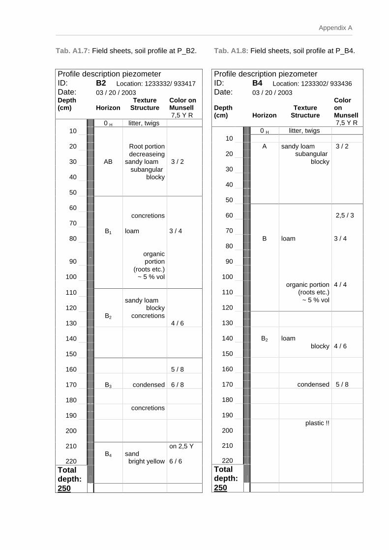
Appendix A
Tab. A1.7: Field sheets, soil profile at P_B2.
Profile description piezometer ID: B2 Location: 1233332/ 933417 Date:
03 / 20 / 2003
Depth (cm) Horizon
Texture
Structure Color on Munsell
7,5 Y R
0 H litter, twigs 10
20
Root portion
decreaseing
30
AB sandy loam 3 / 2
subangular
40
blocky
50
60
concretions
70
B1 loam 3 / 4 80
90
organic portion
(roots etc.)
100
~ 5 % vol
110
sandy loam 120
blocky
B2 concretions
130
4 / 6
140
150
160
5 / 8
170
B3 condensed
6 / 8
180
concretions
190
200
210
on 2,5 Y
B4 sand 220
bright yellow
6 / 6 Total depth:
250
Tab. A1.8: Field sheets, soil profile at P_B4.
Profile description piezometer ID: B4 Location: 1233302/ 933436 Date:
03 / 20 / 2003
Depth (cm) Horizon
Texture
Structure
Color on Munsell
7,5 Y R
0 H litter, twigs 10
A sandy loam 3 / 2 20
subangular
blocky
30
40
50
60
2,5 / 3
70
B loam 3 / 4 80
90
100
organic portion
4 / 4 110
(roots etc.)
~ 5 % vol
120
130
140
B2 loam
blocky
4 / 6 150
160
170
condensed
5 / 8
180
190
plastic !!
200
210
220
Total depth:
250

Appendix A
Tab. A1.9: Field sheets, soil profile at P_C1.
Profile description piezometer ID: C1 Location: 1233342/ 933401 Date:
12 / 19 / 2002
Depth (cm) Horizon
Texture
Structure Color on Munsell
7,5 Y R
0 H litter, twigs 10
A sandy loam 3 / 4
20
30
AB loam 40
subangular
blocky
50
3 / 3
60
70
B1
80
90
B2 loam 4 / 4 100
blocky
110
120
plastic
130
140
150
160
170
180
190
200
210
220
Total depth:
141
Tab. A1.10: Field sheets, soil profile at P_C3.
Profile description piezometer ID: C3 Location: 1233314/ 933413 Date:
12 / 19 / 2002
Depth (cm) Horizon
Texture Structure
Color on Munsell
7,5 Y R
0 H litter, 10
sandy
A loam 2,5 / 2 20
crumbly
30
sandy 40
loam
AB 3 / 2 50
subang.
blocky
60
70
80
90
B loam 3 / 3
100
blocky
110
120
130
140
150
160
170
180
190
200
210
220
Total depth:
114
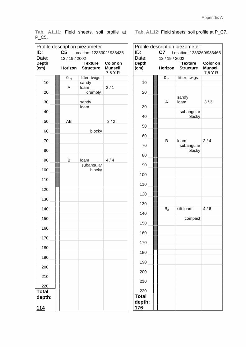
Appendix A
Tab. A1.11: Field sheets, soil profile at P_C5.
Profile description piezometer ID: C5 Location: 1233302/ 933435 Date:
12 / 19 / 2002
Depth (cm) Horizon
Texture
Structure Color on Munsell
7,5 Y R
0 H litter, twigs
10
sandy
A loam 3 / 1 20
crumbly
30
sandy
loam 40
50
AB 3 / 2
60
blocky
70
80
90
B loam 4 / 4
subangular
100
blocky
110
120
130
140
150
160
170
180
190
200
210
220
Total depth:
114
Tab. A1.12: Field sheets, soil profile at P_C7.
Profile description piezometer ID: C7 Location: 1233269/933466
Date:
12 / 19 / 2002
Depth (cm) Horizon
Texture
Structure Color on Munsell
7,5 Y R
0 H litter, twigs 10
20
A sandy loam 3 / 3
30
subangular
40
blocky
50
60
B loam 3 / 4 70
subangular
blocky
80
90
100
110
120
130
B2 silt loam 4 / 6 140
compact
150
160
170
180
190
200
210
220
Total depth:
176

Appendix A
Tab. A1.13: Field sheets, soil profile at P_C9.
Profile description piezometer ID: C9 Location: 1233263/ 933493 Date:
12 / 19 / 2002
Depth (cm)
Horizon
Texture Structure
Color on Munsell
7,5 Y R
0 H litter, twigs 10
sandy loam
A Subangular
3 / 1 20
blocky
30
40
loam 50
B 3 / 4
60
blocky
friable
70
80
90
B2 loam 4 / 6
100
blocky
110
120
130
140
150
160
170
180
190
200
210
220
Total depth:
112
Tab. A1.14: Field sheets, soil profile at P_D1.
Profile description piezometer ID: D1 Location: 1233316/ 933389 Date:
03 / 20 / 2003
Depth (cm) Horizon
Texture
Structure
Color on Munsell
7,5 Y R
0 H litter, twigs 10
A sandy loam 3 / 1 20
subangular
blocky
30
40
B sandy loam 3 / 4 50
blocky
60
friable
70
80
90
100
110
120
130
140
150
160
170
180
190
200
B/C 6 / 8 210
220
Total depth:
230

Appendix A
Tab. A1.15: Field sheets, soil profile at P_D3.
Profile description piezometer ID: D3 Location: 1233290/ 933383
Date:
03 / 20 / 2003
Depth (cm) Horizon
Texture
Structure Color n Munsell
7,5 Y R
0 H litter, twigs 10
3 / 1 20
root portion decreaseing
30
AB sandy loam 3 / 2
subangular
40
blocky
50
60
concretions
70
B1 loam 3 / 3 80
90
~ 5 % vol
100
110
sandy loam 120
blocky
B2
130
5 / 8
concretions
140
(OD = 2mm)
150
160
170
B3 sandy loam
180
190
concretions
200
210
220
Total depth:
230
Tab. A1.16: Field sheets, soil profile at P_D5.
Profile description piezometer ID: D5 Location: 1233284/ 933437 Date:
03 / 20 / 2003
Depth (cm) Horizon
Texture
Structure Color on Munsell
7,5 Y R
0 H litter, twigs 10
sandy
A loam 3 / 1 20
subangular
blocky
30
40
B sandy loam 3 / 4 50
blocky
60
70
80
90
100
110
120
130
140
150
160
170
180
190
200
B/C friable
6 / 8 210
220
Total depth:
230
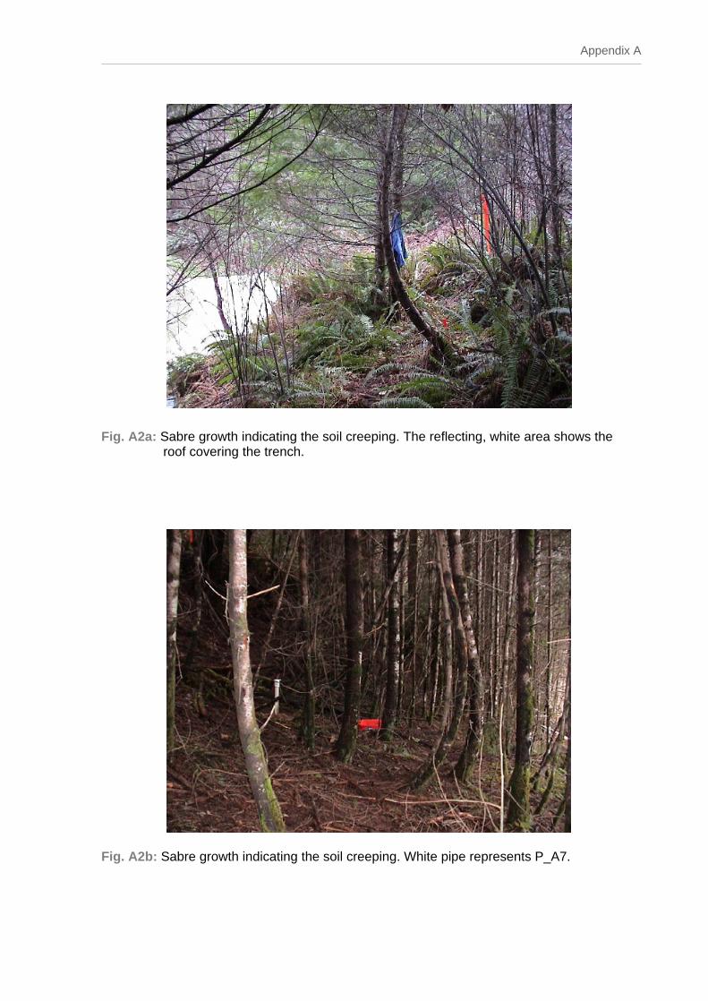
Appendix A
Fig. A2a: Sabre growth indicating the soil creeping. The reflecting, white area shows the roof covering the trench.
Fig. A2b: Sabre growth indicating the soil creeping. White pipe represents P_A7.

Appendix A
Tab. A3: Exact data on hydrograph separation for selected runoff events. Peak
ID Starting
point Time Digitime Ending
point Time Digitime Total
flow [m³]
Method Event flow [m³]
1
17-Feb-03
13:30
-43.4375
20-Feb-03
02:50
-40.8819
165
blip 74
2+3
6-Mar-03
19:50
-26.1736
12-Mar-03
14:20
-20.4028
807
blip 446
4
21-Mar-03
01:00
-11.9583
26-Mar-03
06:40
-6.72222
932
blip 535
4+5
21-Mar-03
01:00
-11.9583
29-Mar-03
13:40
-3.43056
1313
blip 760
6
5-Apr-03
15:40
3.65277
12-Apr-03
01:00
10.0417
523
horiz. Line; * 152
7
23-Apr-03
21:00
21.875
1-May-03
10:30
29.4375
315
horiz. line 87
*) The hydrograph separation of peak ID 6 was done for the period up to digital time 10.0417 although little precipitation was recorded in between. This is visualised in Fig. A3. The included error might still be less dominant compared to the method of separation (e.g. hypothesis of vertical line).
4 5 6 7 8 9 10 114.5 5.5 6.5 7.5 8.5 9.5 10.5
No.
of
days,
relative
to
tracer
application
on
April,2
20
40
60
80
100
120
Tot
al d
isch
arge
soi
l pip
es [l
/10
min
]
1.91.81.71.61.51.41.31.21.110.90.80.70.60.50.40.30.20.10
Thr
ougf
all
prec
ipita
tion
[mm
/10m
in]
4 5 6 7 8 9 10 114.5 5.5 6.5 7.5 8.5 9.5 10.5
Fig. A3: Discharge soil pipes and rain events for the period of hydrograph separation.
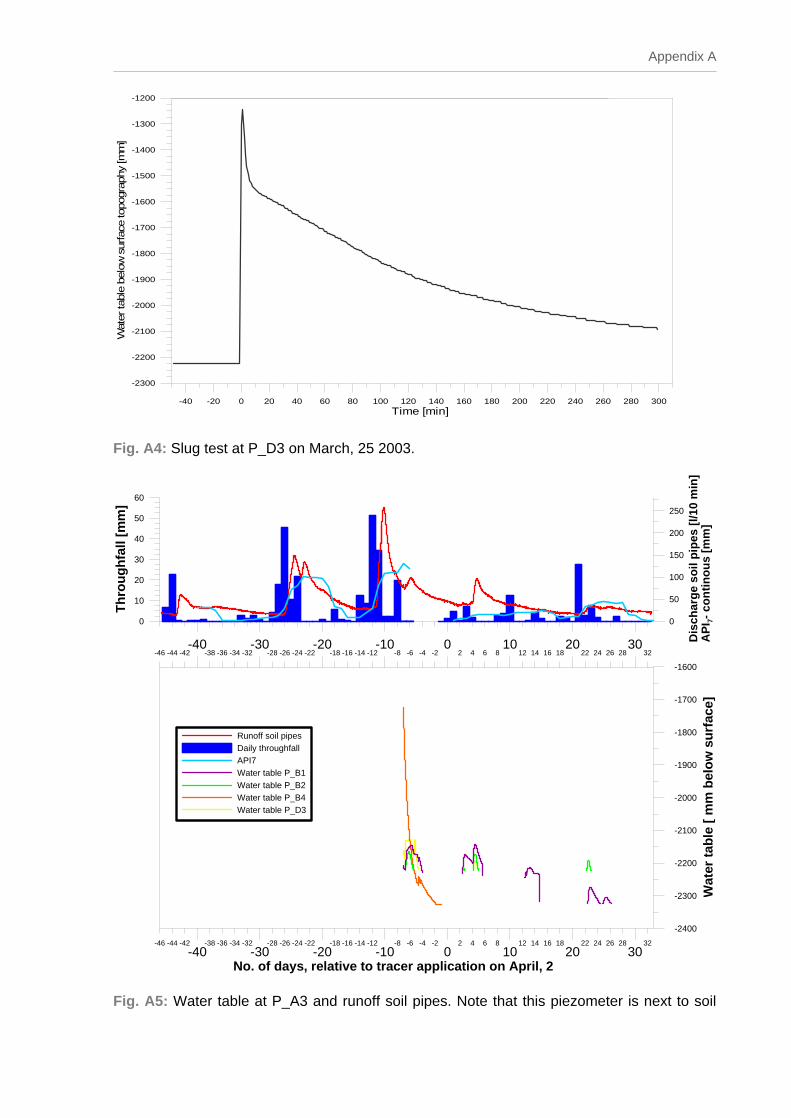
Appendix A
-40 -20 0 20 40 60 80 100 120 140 160 180 200 220 240 260 280 300Time
[min]
-2300
-2200
-2100
-2000
-1900
-1800
-1700
-1600
-1500
-1400
-1300
-1200
Wat
er ta
ble
bel
ow sur
face
topo
grap
hy [m
m]
Fig. A4: Slug test at P_D3 on March, 25 2003.
-40 -30 -20 -10 0 10 20 30-46 -44 -42 -38 -36 -34 -32 -28 -26 -24 -22 -18 -16 -14 -12 -8 -6 -4 -2 2 4 6 8 12 14 16 18 22 24 26 28 32
No. of days, relative to tracer application on April, 2
-2400
-2300
-2200
-2100
-2000
-1900
-1800
-1700
-1600
Wat
er
tab
le
[
mm
bel
ow
surf
ace]
-40 -30 -20 -10 0 10 20 30-46 -44 -42 -38 -36 -34 -32 -28 -26 -24 -22 -18 -16 -14 -12 -8 -6 -4 -2 2 4 6 8 12 14 16 18 22 24 26 28 32
0
10
20
30
40
50
60
Th
rou
gh
fall
[m
m]
0
50
100
150
200
250
Dis
char
ge
soil
pip
es [
l/10
min
]A
PI 7
- co
nti
no
us
[mm
]
Runoff soil pipesDaily throughfallAPI7Water table P_B1Water table P_B2Water table P_B4Water table P_D3
Fig. A5: Water table at P_A3 and runoff soil pipes. Note that this piezometer is next to soil

Appendix A
pipes.
0 50 100 150 200 250 300Pipe flow [l/10 min]
-1200
-1100
-1000
-900
-800
-700
-600
-500W
ater
ta
ble
b
elo
w
su
rfac
e
[m
m]
P_A5P_A9P_C9
Fig. A6: Correlation between water table and pipe flow for selected piezometers.
Tab. A4: Determination of input mass for Low Pass experiment.
Tracer Conzentration, wanted [ppb]
Total flow volume*
[m³]
Tracer mass [g]
Portion of initial mobilisation [%]
Tracer mass [g]
Amino G Acid; line source
100 807 80.7 53 150
Bromide; areal application 10 807 8070 100 8000
* For expected upcoming event similar ID 2+3, according to Tab. A3.
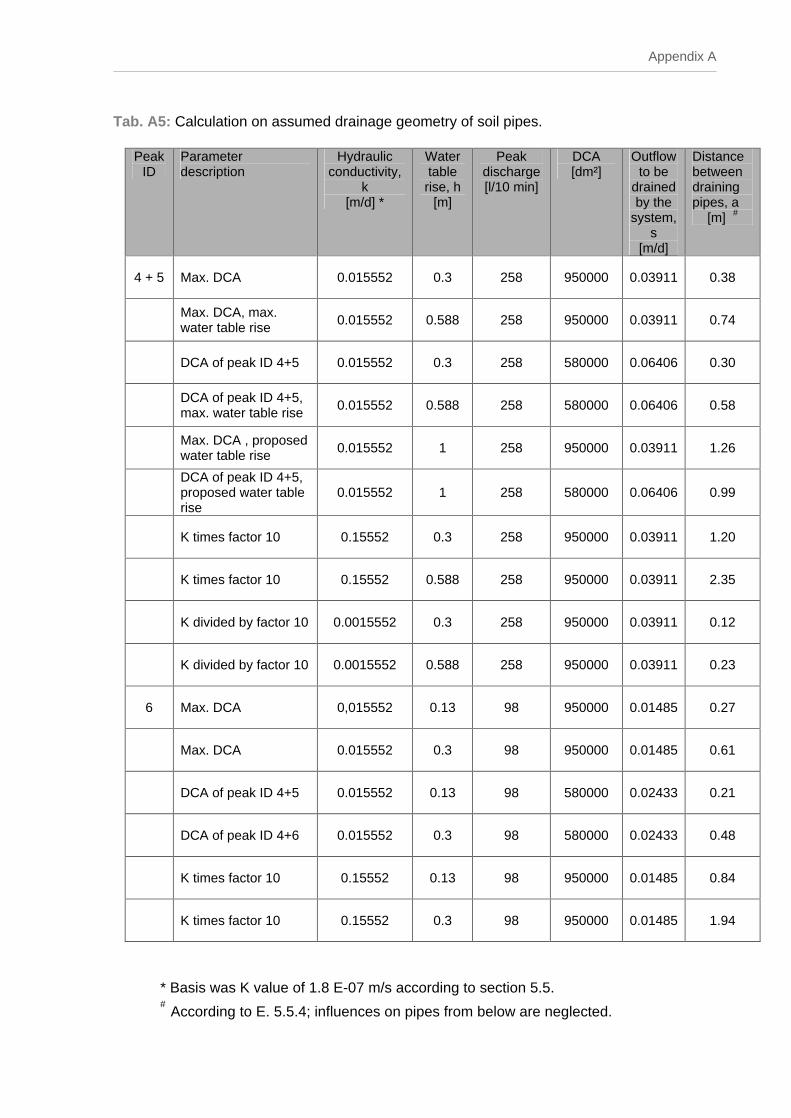
Appendix A
Tab. A5: Calculation on assumed drainage geometry of soil pipes.
Peak ID
Parameter description
Hydraulic conductivity,
k [m/d] *
Water table rise, h
[m]
Peak discharge [l/10 min]
DCA [dm²]
Outflow to be
drained by the
system, s
[m/d]
Distance between draining pipes, a
[m] #
4 + 5 Max. DCA 0.015552 0.3 258 950000 0.03911
0.38
Max. DCA, max. water table rise 0.015552 0.588 258 950000 0.03911
0.74
DCA of peak ID 4+5 0.015552 0.3 258 580000 0.06406
0.30
DCA of peak ID 4+5, max. water table rise 0.015552 0.588 258 580000 0.06406
0.58
Max. DCA , proposed water table rise 0.015552 1 258 950000 0.03911
1.26
DCA of peak ID 4+5, proposed water table rise
0.015552 1 258 580000 0.06406
0.99
K times factor 10 0.15552 0.3 258 950000 0.03911
1.20
K times factor 10 0.15552 0.588 258 950000 0.03911
2.35
K divided by factor 10 0.0015552 0.3 258 950000 0.03911
0.12
K divided by factor 10 0.0015552 0.588 258 950000 0.03911
0.23
6 Max. DCA 0,015552 0.13 98 950000 0.01485
0.27
Max. DCA 0.015552 0.3 98 950000 0.01485
0.61
DCA of peak ID 4+5 0.015552 0.13 98 580000 0.02433
0.21
DCA of peak ID 4+6 0.015552 0.3 98 580000 0.02433
0.48
K times factor 10 0.15552 0.13 98 950000 0.01485
0.84
K times factor 10 0.15552 0.3 98 950000 0.01485
1.94
* Basis was K value of 1.8 E-07 m/s according to section 5.5. #
According to E. 5.5.4; influences on pipes from below are neglected.

Appendix B
Appendix B Data and information for the experimental hillslope table

Appendix B
Tab. B1: Information on irrigation intervals during experiments at hillslope table. Event ID Status Digitime Date Time Sprinkling [mm]
1 on 19.45139 May, 19 1050 2.219 off 19.45486 May, 19 1055
2 on 19.46181 May, 19 1105 2.195 off 19.46528 May, 19 1110
3 on 19.47222 May, 19 1120 2.717 off 19.47569 May, 19 1125
4 on 19.48264 May, 19 1135 2.073 off 19.48611 May, 19 1140
5 on 19.49306 May, 19 1150 2.364 off 19.49653 May, 19 1155
6 on 19.50347 May, 19 1205 2.195 off 19.50694 May, 19 1210
7 on 19.62847 May, 19 1505 2.243 off 19.63194 May, 19 1510
8 on 19.63889 May, 19 1520 2.000 off 19.64236 May, 19 1525
9 on 19.64931 May, 19 1535 2.000 off 19.65278 May, 19 1540
10 on 19.65972 May, 19 1550 1.952 off 19.66319 May, 19 1555
11 on 19.75 May, 19 1800 2.437 off 19.75347 May, 19 1805
12 on 19.76042 May, 19 1815 2.098 off 19.76389 May, 19 1820
13 on 20.49653 May, 20 1155 2.534 off 20.5 May, 20 1200
14 on 20.50694 May, 20 1210 2.340 off 20.51042 May, 20 1215
15 on 20.51736 May, 20 1225 2.825 off 20.52083 May, 20 1230
16 on 20.53472 May, 20 1250 2.389 off 20.53819 May, 20 1255
17 on 20.54514 May, 20 1305 2.389 off 20.54861 May, 20 1310
18 on 20.55903 May, 20 1325 2.098 off 20.5625 May, 20 1330
19 on 20.66806 May, 20 1602 2.146 off 20.67153 May, 20 1607
20 on 20.67847 May, 20 1617 2.146 off 20.68194 May, 20 1622
21 on 20.69444 May, 20 1640 2.146 off 20.69792 May, 20 1645
22 on 20.70486 May, 20 1655 2.049 off 20.70833 May, 20 1700
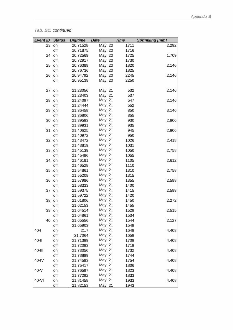
Appendix B
Tab. B1: continued Event ID Status Digitime Date Time Sprinkling [mm]
23 on 20.71528 May, 20 1711 2.292 off 20.71875 May, 20 1716
24 on 20.72569 May, 20 1725 1.709 off 20.72917 May, 20 1730
25 on 20.76389 May, 20 1820 2.146 off 20.76736 May, 20 1825
26 on 20.94792 May, 20 2245 2.146 off 20.95139 May, 20 2250
27 on 21.23056 May, 21 532 2.146 off 21.23403 May, 21 537
28 on 21.24097 May, 21 547 2.146 off 21.24444 May, 21 552
29 on 21.36458 May, 21 850 3.146 off 21.36806 May, 21 855
30 on 21.39583 May, 21 930 2.806 off 21.39931 May, 21 935
31 on 21.40625 May, 21 945 2.806 off 21.40972 May, 21 950
32 on 21.43472 May, 21 1026 2.418 off 21.43819 May, 21 1031
33 on 21.45139 May, 21 1050 2.758 off 21.45486 May, 21 1055
34 on 21.46181 May, 21 1105 2.612 off 21.46528 May, 21 1110
35 on 21.54861 May, 21 1310 2.758 off 21.55208 May, 21 1315
36 on 21.57986 May, 21 1355 2.588 off 21.58333 May, 21 1400
37 on 21.59375 May, 21 1415 2.588 off 21.59722 May, 21 1420
38 on 21.61806 May, 21 1450 2.272 off 21.62153 May, 21 1455
39 on 21.64514 May, 21 1529 2.515 off 21.64861 May, 21 1534
40 on 21.65556 May, 21 1544 2.127 off 21.65903 May, 21 1549 40-I on 21.7 May, 21 1648 4.408 off 21.7064 May, 21 1658 40-II on 21.71389 May, 21 1708 4.408 off 21.72083 May, 21 1718 40-III on 21.73056 May, 21 1732 4.408 off 21.73889 May, 21 1744 40-IV on 21.74583 May, 21 1754 4.408 off 21.75417 May, 21 1806 40-V on 21.76597 May, 21 1823 4.408 off 21.77292 May, 21 1833 40-VI on 21.81458 May, 21 1933 4.408 off 21.82153 May, 21 1943

Appendix B
20 21 2219.4 19.6 19.8 20.2 20.4 20.6 20.8 21.2 21.4 21.6 21.8 22.2 22.4
Digital time
0
100
200
300
400
500
600
700
800
900
1000
Dis
char
ge a
t TB
1[m
l/2 m
in]
60
50
40
30
20
10
0
6462
58565452
48464442
38363432
28262422
18161412
8642
Spr
inkl
ing
[mm
] // A
min
o-G
con
cent
ratio
n at
TB
1 [µ
g/l]
20 21 2219.4 19.6 19.8 20.2 20.4 20.6 20.8 21.2 21.4 21.6 21.8 22.2 22.4
SprinklingDischargeAmino G conc.
Fig. B1: Amino G breakthrough, accumulated discharge and sprinkling intervals at TB 1.
20 21 2219.4 19.6 19.8 20.2 20.4 20.6 20.8 21.2 21.4 21.6 21.8 22.2 22.4
Digital time
0
100
200
300
400
500
600
700
800
900
1000
Dis
char
ge a
t TB
2[m
l/2 m
in]
60
50
40
30
20
10
0
6462
58565452
48464442
38363432
28262422
18161412
8642
Spr
inkl
ing
[mm
] // A
min
o-G
con
cent
ratio
n at
TB
2 [µ
g/l]
20 21 2219.4 19.6 19.8 20.2 20.4 20.6 20.8 21.2 21.4 21.6 21.8 22.2 22.4
SprinklingDischargeAmino G conc.
Fig. B2: Amino G breakthrough, accumulated discharge and sprinkling intervals at TB 2.
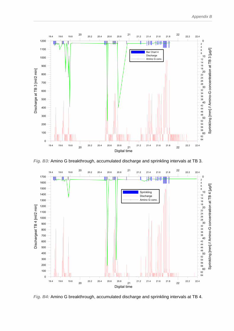
Appendix B
20 21 2219.4 19.6 19.8 20.2 20.4 20.6 20.8 21.2 21.4 21.6 21.8 22.2 22.4
Digital time
0
100
200
300
400
500
600
700
800
900
1000
1100
1200
Dis
char
ge a
t TB
3 [m
l/2 m
in]
60
50
40
30
20
10
0
6462
58565452
48464442
38363432
28262422
18161412
8642
Spr
inkl
ing
[mm
] // A
min
o-G
con
cent
ratio
n at
TB
3 [µ
g/l]
20 21 2219.4 19.6 19.8 20.2 20.4 20.6 20.8 21.2 21.4 21.6 21.8 22.2 22.4
Bar Chart 4DischargeAmino G conc.
Fig. B3: Amino G breakthrough, accumulated discharge and sprinkling intervals at TB 3.
20 21 2219.4 19.6 19.8 20.2 20.4 20.6 20.8 21.2 21.4 21.6 21.8 22.2 22.4
Digital time
0
100
200
300
400
500
600
700
800
900
1000
1100
1200
1300
1400
1500
1600
1700
Dis
char
geat
TB
4 [m
l/2 m
in]
60
50
40
30
20
10
0
6462
58565452
48464442
38363432
28262422
18161412
8642
Spr
inkl
ing
[mm
] // A
min
o-G
con
cent
ratio
n at
TB
4 [µ
g/l]
20 21 2219.4 19.6 19.8 20.2 20.4 20.6 20.8 21.2 21.4 21.6 21.8 22.2 22.4
SprinklingDischargeAmino G conc.
Fig. B4: Amino G breakthrough, accumulated discharge and sprinkling intervals at TB 4.

Appendix B
20 21 2219.4 19.6 19.8 20.2 20.4 20.6 20.8 21.2 21.4 21.6 21.8 22.2 22.4
Digital time
0
100
200
300
400
500
600
700
800
900
1000
Dis
char
ge a
t TB
5 [m
l/2 m
in]
90
80
70
60
50
40
30
20
10
0
88868482
78767472
68666462
58565452
48464442
38363432
28262422
18161412
8642
Spr
inkl
ing
[mm
] // A
min
o-G
con
cent
ratio
n at
TB
5 [µ
g/l]
20 21 2219.4 19.6 19.8 20.2 20.4 20.6 20.8 21.2 21.4 21.6 21.8 22.2 22.4
SprinklingDischargeAmino G conc.
Fig. B5: Amino G breakthrough, accumulated discharge and sprinkling intervals at TB 5.
20 21 2219.4 19.6 19.8 20.2 20.4 20.6 20.8 21.2 21.4 21.6 21.8 22.2 22.4
Digital time
0
100
200
300
400
500
600
700
800
900
1000
1100
1200
1300
1400
1500
1600
Dis
char
ge a
t TB
6 [m
l/2 m
in]
60
50
40
30
20
10
0
6462
58565452
48464442
38363432
28262422
18161412
8642
Spr
inkl
ing
[mm
] // A
min
o-G
con
cent
ratio
n at
TB
6 [µ
g/l]
20 21 2219.4 19.6 19.8 20.2 20.4 20.6 20.8 21.2 21.4 21.6 21.8 22.2 22.4
Bar Chart 4DischargeAmino G conc.
Fig. B6: Amino G breakthrough, accumulated discharge and sprinkling intervals at TB 6.

Appendix B
20 21 2219.4 19.6 19.8 20.2 20.4 20.6 20.8 21.2 21.4 21.6 21.8 22.2 22.4
Digital time
0
100
200
300
400
500
600
700
800
900
1000D
isch
arge
at T
B 7
[ml/2
min
]
60
50
40
30
20
10
0
6462
58565452
48464442
38363432
28262422
18161412
8642
Spr
inkl
ing
[mm
] // A
min
o-G
con
cent
ratio
n at
TB
7 [µ
g/l]
20 21 2219.4 19.6 19.8 20.2 20.4 20.6 20.8 21.2 21.4 21.6 21.8 22.2 22.4
SprinklingRunoffAmino G conc.
Fig. B7: Amino G breakthrough, accumulated discharge and sprinkling intervals at TB 7.
0 10 20 30 40 50 60 70 80 90 100 110 1EC [µS / cm]
20
0
10
20
30
40
Flow
pro
porti
onal
sam
ples
;B
rom
ide
conc
entra
tion
[mg
/ l]
Y = 0.2780 * X - 7.0850R² = 0.4875
Fig. B8: Correlation between electrical conductivity and bromide concentration of flow proportional hand samples at TB 1.

Appendix B
0 10 20 30 40 50 60 70 80 90 100 110 1EC [µS / cm]
20
0
10
20
30
40
Flow
pro
porti
onal
sam
ples
;B
rom
ide
conc
entra
tion
[mg
/ l]
Y = 0.3227 * X - 7.3905R² = 0.729
Fig. B9: Correlation between electrical conductivity and bromide concentration of flow proportional hand samples at TB 1, for the times < 19.5.
0 10 20 30 40 50 60 70 80 90 100 110 1EC [µS / cm]
20
0
10
20
30
40
Flow
pro
porti
onal
sam
ples
;B
rom
ide
conc
entra
tion
[mg
/ l]
Y = 0.1947 * X - 0.4715R² = 0.1196
Fig. B10: Correlation between electrical conductivity and bromide concentration of flow proportional hand samples at TB 8.

Appendix B
20 21 2219.4 19.6 19.8 20.2 20.4 20.6 20.8 21.2 21.4 21.6 21.8 22.2 22.4
Digital time
0
20
40
60
80
100
120
140
160
180
200
220
240
260A
ccum
ulat
ed d
isch
arge
at T
B 8
[l]
0
10
20
30
40
50
60
Sprin
klin
g [m
m ]
Bro
mid
e co
ncen
trat
ion
at T
B 8
[mg/
l] EC
at T
B 8
[mS/
cm]
20 21 2219.4 19.6 19.8 20.2 20.4 20.6 20.8 21.2 21.4 21.6 21.8 22.2 22.4
SprinklingAccumulated QBromide concentration (samples)EC at TB 8
Fig. B11: Bromide concentrations, electrical conductivity, sprinkling intervals and accumulated discharge at TB 8.

Appendix C
Appendix C Technical information

Appendix C
C1 Tipping buckets
Fig. C1: Sketch of tipping buckets to provide a visual impression for information purposes. The drawing is intentionally simplified and includes only includes the most
functional details. C2 Piezometer This data logger offers high solution data in either two channel (old models) or three channel modes. In this study (with two exceptions due to availability) the more recent ones were used. The channels of these relate to water height, water temperature and air temperature. The sensor type of the water table recorders is capacitive. Operation is effective within the temperature range of 0°C to +70°C (TRUTRACK, 2003). Within that, the accuracy equals
± 1 mm. Piezometers of various lengths are available. In this study the WT-HR 500 (500 mm rod length measurable; total length: 820 mm) was used for the table experiment and the WT-HR 1000, WT-HR 1500 for the field experiments.
The data transfer by Omnilog software offers automatic temperature correction, in case channel water temperature and air temperature are is online. The dependent relationship of

Appendix C
water height for a water column of 1000 mm is a 0.65 mm decrease by increasing water temperature by 1 °C. Another error is connected with air temperature. According to the manufacture (TRUTRACK, 2003), the water height increases by 0.5 mm (starting at the offset / base level 0 mm) if the air temperature increases by 1 °C. WT-HR data loggers are easy to handle, and they will even download reliably under rough weather conditions. The memory of the logger is large enough for intensive field campaigns. A three channel mode by 10 min intervals runs about two months. This implements for the 12 bit high resolution mode a memory capacity of 32000 samples (TRUTRACK, 2003). The body of the logger is made out of solid stainless steel (Fig. C2a). Vibrations during transport (car driving) prior to installation were once the reason for a lost plugging connection between tub and middle rod. Therefore a compulsory check should be done before installing the capacity rods in the field. Unfortunately there is no possibility of receiving raw data (simply voltage) from the logger. This may be an issue for self-adopted calibration on specific local conditions (particular water with its electrical conductivity, range in water and air temperature etc.). However, the data obtained in this study are all corrected for the temperature error automatically.
Fig. C2a: Water height recorder WT-HR. From: TRUTRACK (2003). From the bottom end of the piezometers until the offset (reading zero) is a range of 74 mm. This means that the logger needs an established water table of at least that height in the pipe to provide results. Less than that the data were not reliable. Finally the result of the measurements shows water level in depth below surface. The water table recorder is housed in a PVC-pipe, shown in Fig. C2b. For the purpose of sediment protection the slits are covered with gauze, as mentioned earlier. Early on the PVC-pipe was placed again in a drill hole. After positioning the pipe in the lower part of the left drill hole is refilled by sand. Afterwards soil follows, and after that, as a protection against passing water from the upper zones, the pipes are surrounded by a dense layer of bentonit. Finally, up to the surface there is some heavy dense soil again. The data logger was lowered in the pipe connected by a rope to the lid of the pipe (see horizontal axis in Fig. C2b). The pipe is protected by a closed lid except during maintenance and during insertion.
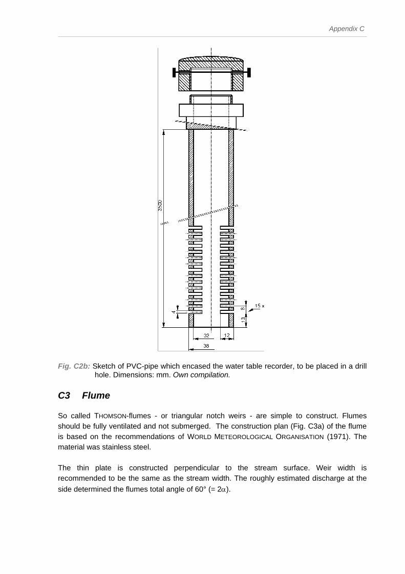
Appendix C
Fig. C2b: Sketch of PVC-pipe which encased the water table recorder, to be placed in a drill
hole. Dimensions: mm. Own compilation.
C3 Flume So called THOMSON-flumes - or triangular notch weirs - are simple to construct. Flumes should be fully ventilated and not submerged. The construction plan (Fig. C3a) of the flume is based on the recommendations of WORLD METEOROLOGICAL ORGANISATION (1971). The material was stainless steel. The thin plate is constructed perpendicular to the stream surface. Weir width is recommended to be the same as the stream width. The roughly estimated discharge at the
side determined the flumes total angle of 60° (= 2α).
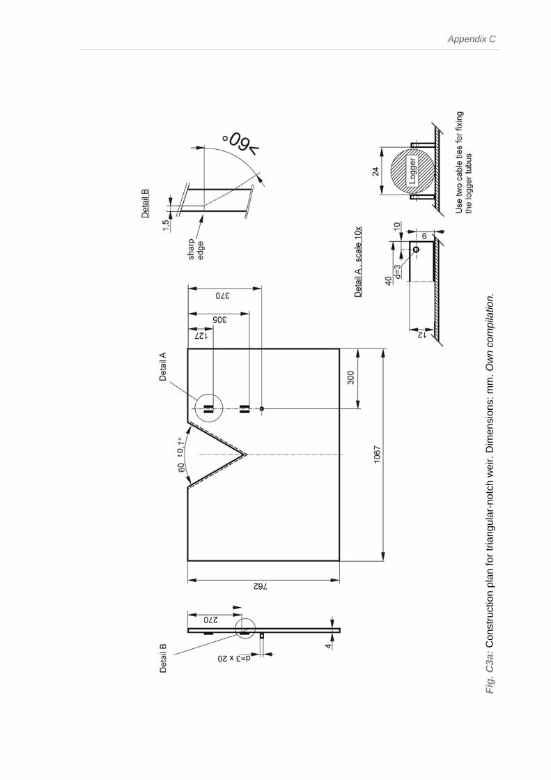
Appendix C
Fig
. C3a
: C
onst
ruct
ion
plan
for
tria
ngul
ar-n
otch
wei
r. D
imen
sion
s: m
m. O
wn
com
pila
tion.

Appendix C
The discharge can be calculated for these kinds of weirs, using an integrating approach. The deviation necessary for determinations are shown in Fig. C3b.
Fig. C3b: Details of notch. Modification of: RÖSSERT (1981). According to that the general calculation for a “v“-shaped flume is (after RÖSSERT, 1981):
( ) ( )
( ) ( )
( ) 250
0
230
00
tan2158
dtan22
dtan22
0
0
hg
hhhhg
hhhhgQ
h
h
VFlume
αµ
αµ
αµ
=
−=
−=
∫
∫
(E. C-1)
where: QVFlume = discharge “v”-shaped flume [m³/s] µ = coefficient [-] g = gravity [m/s²] h0 = water height above notch [m]
α = angle ½ notch [°] In this study the flume is calibrated in a classical way by volumetric gauging of the discharge per time. This process needed a small barrel measuring at two minutes, which is later multiplied for a 10 minutes value. According to that the coefficient µ is set to a constant 0.644. This is in agreement with the theoretical coefficient published by SCHRÖDER (1994), where µ is about 0.64 for a fully ventilated, sharp-edged overfall. Based on this, discharge was calculated by the formula, which provides the rating curve in this case. For an illustration of the rating curve of the flume see Fig. C3c. To understand this graphic, two facts are important: first the gauging on May, 23 is admittedly wrong, as it does not fit in the theoretical context (indicated by an error bar of 61 %, within which the regression would fit). This was certainly a procedural mistake. The minimal change of the coefficient µ in lower heights of the “v”-shape, a circumstance mentioned by SCHRÖDER (1994), would not result in such a deviation. Second, the data processing is difficult. Very often the rating is wrong,

Appendix C
because of clogging up by branches. Therefore, the rating curve presented in Fig. C3c does not last for the total series but definitely for the first measured peak.
0 100 200 300 400 500 600 700 800 900Discharge [l / 10 min]
0
0.01
0.02
0.03
0.04
0.05
0.06
0.07
0.08
Wat
er h
eigh
t [m
]
rating curve for discharge >184 l/10 min; µ=0,644calibration on April, 5 (18:50 h) and April, 14 (11:50h) calibration on May, 23 (13:00h) with error bar
Fig. C3c: Rating curve of “v”-notched weir.

Appendix C
C4 Lysimeter The lysimeter instrument consisting of a tube, a head with a locking aperture, and a bottom, is described in Fig. C4. Most functional is the porous ceramic cup which allows the water to pass through in case of an inside vacuum. The installation of suction lysimeters is essential for efficient water collection later on. This operation was based on PARIZEK & LANE (1970). Best results are obtained by pushing the bottom end of the lysimeter into a slurry remaining in the cored hole. The consistency of cement mortar provides the best soil contact with the porous ceramic cup. The remaining area around the sampler is later on backfilled with soil. As for the piezometers it is important to tamp soil firmly to prevent surface water from running down the cored hole.
Fig. C4: Sketch of soil water sampler. Adapted from: Soilmoisture Equipment Corporation.

Appendix C
C5 Electrical conductivity probes The body of the probe is a PVC-pipe, which serves as a reservoir at the upper side, where the water is measured. The lower part with the electrics was sealed completely by synthetic resin. This contained two circuits, one for electrical conductivity and another one for temperature levelling. Therefore all the conductivity values were temperature corrected. For circuit diagram and wiring instructions for the CAMPBELL data logger see Fig. C5. The shortcuts refer to corresponding input locations at the logger (excitation, high, and ground). A calibration with standard solutions set the conductivity reliably.
Fig. C5: Sketch and circuit diagram of electrical conductivity probe. Dimensions: mm.
Own compilation. C6 Mini-wells for water sampling at table Obvious similarities between the mini-wells and the piezometer in the field are shown in Fig. C6. The mini-wells are built out of PVC pipes, a rubber stopper, a tiny lid and a piece of elastic rubber hose. Not shown in the figure is the medical gauze around the slits for sediment protection. The foundation for the sampling tube is the ground of the table. This means there is a direct fit to the table. At the top of the mini well, the rubber hose runs up to a medical syringe (model: 20 ml content). Here the water samples are sucked into the syringe. Mini wells were included in the soil after levelling.
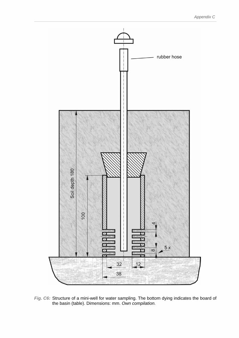
Appendix C
Fig. C6: Structure of a mini-well for water sampling. The bottom dying indicates the board of
the basin (table). Dimensions: mm. Own compilation.

Appendix C
C7 Program code for throughfall-data disaggregation Macro program code, running in MS EXCEL
©:
Dim start_time, end_time, timestep, tipval As Double 'days - max65536 steps Dim counter Dim data(0 To 65536) As Double 'Julian days - tip times Dim bindata(1 To 65536, 1 To 2) As Double 'bin, start_time, volume Sub main() Sheets("output_data").Range("a:b").Clear start_time = Sheets("program").Cells(4, 2) end_time = Sheets("program").Cells(5, 2) timestep = Sheets("program").Cells(7, 2) tipval = Sheets("program").Cells(9, 2) If (end_time - start_time) / timestep > 65536 Then Sheets("output_data").Cells(1, 1) = "OUTPUT ARRAY OVERFLOW" Exit Sub End If 'create array of data counter = 1 Do Until Sheets("input_data").Cells(counter, 1) = 0 data(counter) = Sheets("input_data").Cells(counter, 1) counter = counter + 1 Loop 'choose algorithm and execute If Sheets("program").Cells(12, 2) = 1 Then binclick Else bincont 'write out data counter = 1 Do Until bindata(counter, 1) = 0 For a = 1 To 2 Sheets("output_data").Cells(counter, a) = bindata(counter, a) Next a If bindata(counter, 2) = 0 Then Sheets("output_data").Cells(counter, 2) = 0 counter = counter + 1 Loop End End Sub Function binclick() countdata = 1 countbin = 1 'ignore data before start_time Do Until Sheets("input_data").Cells(countdata, 1) >= start_time countdata = countdata + 1 Loop Do Until start_time >= end_time 'add data to current bin bindata(countbin, 1) = start_time Do Until data(countdata) >= start_time + timestep bindata(countbin, 2) = bindata(countbin, 2) + tipval countdata = countdata + 1 If countdata = counter Then Exit Do If countin = counter Then Exit Do Loop

Appendix C
If countdata = counter Then Exit Do countbin = countbin + 1 start_time = start_time + timestep Loop End Function Function bincont() t1 = start_time t2 = t1 + timestep j = 1 'placeholder in the bindata array a = 1 'placeholder in the data array 'ignore data before the time of interest; get to proper start in data array 'Do Until t1 >= data(a) ' a = a + 1 ' If a > 65536 Then Exit Do 'Loop Do Until j > ((end_time - start_time) / timestep) While t1 >= data(a) a = a + 1 If a > counter Then Exit Do Wend If t2 <= data(a) Then binvol = (tipval / (data(a) - data(a - 1))) * (t2 - t1) ElseIf t2 <= data(a + 1) Then binvol = (tipval / (data(a + 1) - data(a))) * (t2 - data(a)) binvol = binvol + (tipval / (data(a) - data(a - 1))) * (data(a) - t1) Else binvol = (tipval / (data(a) - data(a - 1))) * (data(a) - t1) Do While t2 > data(a + 1) If data(a + 1) = data(a) Then binvol = binvol + tipval Else: binvol = binvol + (tipval / (data(a + 1) - data(a))) * (data(a + 1) - data(a)) End If a = a + 1 If a > counter Then Exit Do Loop If data(a) = 0 Then binvol = 0 Else: binvol = binvol + (tipval / (data(a + 1) - data(a))) * (t2 - data(a)) End If End If bindata(j, 1) = t1 bindata(j, 2) = binvol t1 = t2 t2 = t1 + timestep j = j + 1 ' If j * timestep > end_time - start_time Then Exit Do Loop End Function