
Instability in flow through elastic conduits and volcanic ...njb/Research/xtrem.pdf · Instability...
25
J. Fluid Mech. (2005), vol. 527, pp. 353–377. c 2005 Cambridge University Press DOI: 10.1017/S0022112004002800 Printed in the United Kingdom 353 Instability in flow through elastic conduits and volcanic tremor By NEIL J. BALMFORTH 1,2 , R. V. CRASTER 3 AND A. C. RUST 2 1 Department of Mathematics, University of British Columbia, 1984 Mathematics Road, Vancouver, BC, V6T 1Z2, Canada 2 Department of Earth & Ocean Sciences, University of British Columbia, 6339 Stores Road, Vancouver, BC, V6T 1Z4, Canada 3 Department of Mathematics, Imperial College, London SW7 2BZ, UK (Received 17 March 2004 and in revised form 2 October 2004) The stability of fluid flow through a narrow conduit with elastic walls is explored, treating the fluid as incompressible and viscous, and the walls as semi-infinite linear Hookean solids. Instabilities analogous to roll waves occur in this system; we map out the physical regime in which they are excited. For elastic wave speeds much higher than the fluid speed, a critical Reynolds number is required for instability. However, that critical value depends linearly on wavenumber, and so can be made arbitrarily small for long waves. For smaller elastic wave speeds, the critical Reynolds number is reduced still further, and Rayleigh waves can be destabilized by the fluid even at zero Reynolds number. A brief discussion is given of the nonlinear dynamics of the instabil- ities for large elastic wave speed, and the significance of the results to the phenomenon of volcanic tremor is presented. Although magma itself seems unlikely to generate flow-induced vibrations, the rapid flow through fractured rock of low-viscosity fluids exsolved from magma appears to be a viable mechanism for volcanic tremor. 1. Introduction Sustained ground vibrations are observed at most active volcanoes, and are some- times a precursor to eruptions. This ‘volcanic tremor’ is often found to be distinctly harmonic, and analysis of time series reveals fairly well-defined spectral peaks at periods of seconds (e.g. Julian 1994; Hagerty et al. 2000). The phenomenon is thought to be associated with the subsurface unsteady flow of magma, although the nature and origin of the fluid motions has not yet been determined (Konstantinou & Schlindwein 2002). One theoretical model proposed by Julian (1994) advances the premise that tremor arises from instability in magma conduits owing to interaction between the flowing magma and the surrounding rock. This instability is analogous to that seeding the roll waves which travel on thin falling fluid films and propagate down turbulent water courses (e.g. Chang 1994), and related explanations have been advocated for un- steady blood flow and ‘Korotkov sounds’ in physiology (Pedley 1980; Brook, Pedley & Falle 1999). The destabilization of fluid flow by a compliant wall is a familiar notion in several other branches of fluid mechanics, notably in drag reduction in engineering (Benjamin 1960, 1963; Landahl 1962) and in air flow through passages in the lung (LaRose & Grotberg 1997; Moriarty & Grotberg 1999). In these contexts, the flow is relatively high speed (high Reynolds number), and the compliant walls typically take the form
Transcript of Instability in flow through elastic conduits and volcanic ...njb/Research/xtrem.pdf · Instability...
J. Fluid Mech. (2005), vol. 527, pp. 353–377. c© 2005 Cambridge University Press
DOI: 10.1017/S0022112004002800 Printed in the United Kingdom
353
Instability in flow through elastic conduitsand volcanic tremor
By NEIL J. BALMFORTH1,2, R. V. CRASTER3
AND A. C. RUST2
1Department of Mathematics, University of British Columbia, 1984 Mathematics Road,Vancouver, BC, V6T 1Z2, Canada
2Department of Earth & Ocean Sciences, University of British Columbia, 6339 Stores Road,Vancouver, BC, V6T 1Z4, Canada
3Department of Mathematics, Imperial College, London SW7 2BZ, UK
(Received 17 March 2004 and in revised form 2 October 2004)
The stability of fluid flow through a narrow conduit with elastic walls is explored,treating the fluid as incompressible and viscous, and the walls as semi-infinite linearHookean solids. Instabilities analogous to roll waves occur in this system; we map outthe physical regime in which they are excited. For elastic wave speeds much higherthan the fluid speed, a critical Reynolds number is required for instability. However,that critical value depends linearly on wavenumber, and so can be made arbitrarilysmall for long waves. For smaller elastic wave speeds, the critical Reynolds number isreduced still further, and Rayleigh waves can be destabilized by the fluid even at zeroReynolds number. A brief discussion is given of the nonlinear dynamics of the instabil-ities for large elastic wave speed, and the significance of the results to the phenomenonof volcanic tremor is presented. Although magma itself seems unlikely to generateflow-induced vibrations, the rapid flow through fractured rock of low-viscosity fluidsexsolved from magma appears to be a viable mechanism for volcanic tremor.
1. IntroductionSustained ground vibrations are observed at most active volcanoes, and are some-
times a precursor to eruptions. This ‘volcanic tremor’ is often found to be distinctlyharmonic, and analysis of time series reveals fairly well-defined spectral peaks atperiods of seconds (e.g. Julian 1994; Hagerty et al. 2000). The phenomenon is thoughtto be associated with the subsurface unsteady flow of magma, although the nature andorigin of the fluid motions has not yet been determined (Konstantinou & Schlindwein2002). One theoretical model proposed by Julian (1994) advances the premise thattremor arises from instability in magma conduits owing to interaction between theflowing magma and the surrounding rock. This instability is analogous to that seedingthe roll waves which travel on thin falling fluid films and propagate down turbulentwater courses (e.g. Chang 1994), and related explanations have been advocated for un-steady blood flow and ‘Korotkov sounds’ in physiology (Pedley 1980; Brook, Pedley &Falle 1999).
The destabilization of fluid flow by a compliant wall is a familiar notion in severalother branches of fluid mechanics, notably in drag reduction in engineering (Benjamin1960, 1963; Landahl 1962) and in air flow through passages in the lung (LaRose &Grotberg 1997; Moriarty & Grotberg 1999). In these contexts, the flow is relativelyhigh speed (high Reynolds number), and the compliant walls typically take the form
354 N. J. Balmforth, R. V. Craster and A. C. Rust
of thin tubes or layers. Consequently, much work has gone into understanding theinstability of inviscid or potential flow, and the theory of elastic shells or plates isused to provide boundary conditions at the compliant walls. Instabilities are usuallyfound to arise for flow speeds greater than the natural elastic wave speeds of the wall(Gad-El-Hak, Blackwelder & Riley 1984; Duncan, Waxman & Tulin 1985). By con-trast, in the volcanic problem, the underlying flow of magma is much slower (lowReynolds number), and certainly rather less than the elastic wave speeds in thesurrounding rock. Moreover, the geometry of the volcanic conduit is quite differentbecause the rock occupies a far larger region than the conduit itself. Overall, thesedifferences force us into a separate theoretical discussion of volcanic tremor. A notableexception is the approach taken in the series of papers by Kumaran and collaborators,which bears some similarity to the route followed in the current paper (Kumaran,Fredricksen & Pinkus 1994; Srivatsan & Kumaran 1997; Shankar & Kumaran 2002).
In this regard, although Julian’s model shows that flow instability is a possiblemechanism for tremor, it is based on phenomenological arguments and not derivedfrom the governing equations. That system should consist of fluid equations for themagma and the equations of elasticity for the surrounding solid rock. Consequently,a more quantitative model of volcanic tremor is still desired in order to assess morecompletely whether the flow instability mechanism truly lies at the heart of thephenomenon. Furthermore, a better theoretical model of the phenomena might proveuseful as a tool to aid the prediction of eruptions and other dangerous volcanic events.
The purpose of the present paper is to take the mathematical modelling of Julian’smechanism a step further. In § 2, we analyse the governing equations for an idealizedvolcanic conduit. In particular, in § § 3 and 4, we consider viscous flow along a longuniform conduit sandwiched between two semi-infinite elastic slabs, and study theexcitation of propagating waves, using long-wave expansion and linear stability theory.This approach parallels theory presented for roll waves in other contexts (Brook,Pedley & Falle 1999; Balmforth & Mandre 2004; Balmforth & Liu 2004). We alsobriefly describe results for nonlinear waves, uncovering what appears to be com-plicated spatio-temporal dynamics (§ 5). Overall, the results confirm that Julian’smechanism is plausible, although the physical conditions required for instability seemsomewhat removed from those expected geologically. We offer some remarks placingthe mathematical model into the context of volcanic tremor in our conclusions (§ 6),and mention the main direction of future work.
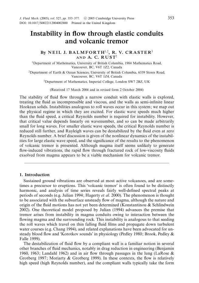
2. Formulation of the modelOur idealization of the physical problem is shown schematically in figure 1. We
consider a conduit, or slot, described by a Cartesian coordinate system in which x
points along the slot and y is perpendicular to it. The magma, contained in −h(x, t) <
y <h(x, t), is treated as a Newtonian viscous fluid, and the surrounding rock as anelastic solid. The slot is relatively narrow, being a crack that is opened by an ambientfluid pressure comparable to the stresses within the rock. The crack supports a flowdriven by a pressure gradient corresponding to a pressure difference that could berather smaller than the ambient pressure. We take the crack to be symmetric abouty = 0, and therefore consider only varicose disturbances.
2.1. The fluid
The fluid is described by an Eulerian coordinate system, (x, y), together with thevelocity field, (u(x, y, t), v(x, y, t)), and pressure, p(x, y, t). The governing equations
Instability in narrow elastic conduits 355
Hh(x, t)
y(a)
(b)
x
Fluid
Elastic solid
Elastic solid
y
x
h(x, t)
Elastic solid
Fluid
u(x, y, t)
v (x, y, t)
H
Y
(X, 0)X
(X + ξ, η)
Figure 1. Idealization of the magma conduit. (a) The geometry of a fluid moving through aconduit bounded by semi-infinite elastic solids. (b) The coordinate systems used to describethe fluid and solid.
are given by conservation of momentum,
ρ(ut + uux + vuy) = −px + ρν(uxx + uyy), (2.1)
ρ(vt + uvx + vvy) = −py + ρν(vxx + vyy) (2.2)
and continuity,
ux + vy = 0, (2.3)
where ρ and ν are the fluid density and viscosity, respectively. The fluid stresses aregiven by the tensor, (
2ρνux − p ρν(uy + vx)
ρν(uy + vx) 2ρνvy − p
). (2.4)
2.2. The elastic solid
The elastic solid is described by a coordinate system, (X, Y ), based on the unstressedsolid arrangement: under the imposed ambient and dynamic stresses, an elasticelement is displaced from the position (X, Y ) to (X + ξ, Y + η), where the displacementfield, ( ξ (X, Y, t), η(X, Y, t)), satisfies the equations of motion,
ρsξtt =∂σXX
∂X+
∂σXY
∂Y, ρsηtt =
∂σXY
∂X+
∂σYY
∂Y, (2.5)
where ρs is the solid density and σIJ denote the components of the elastic stress.
356 N. J. Balmforth, R. V. Craster and A. C. Rust
We take the elastic stress–strain relation to be linear, isotropic and Hookean:
{σIJ } =
((2µ + λ)ξX + ληY µ(ξY + ηX)
µ(ηX + ξY ) (2µ + λ)ηY + λξX
), (2.6)
where λ and µ represent Lame constants, which are related to Poisson’s ratio, � , via� = λ/(2(µ + λ)).
In the volcanic setting, the fluid speeds are far less than the speeds at which elasticwaves propagate in the solid (typically the latter are O(103) m s−1). In this situation,we could drop the acceleration terms from (2.5) so the elastic medium is quasi-static. We give a general discussion of the linear stability of waves propagating in thefluid without making this further simplification, but when considering nonlinear waveswe resort to the quasi-static approximation. Our motivation for the more generaltreatment of the linear stability problem is partly to present a coherent mathematicalanalysis. However, elastic wave speeds in viscoelastic coatings, polymer gels andbiological tissues can be relatively small (as low as centimetres per second – Gad-El-Hak et al. 1984; Moriarty & Grotberg 1999; Muralikrishnan & Kumaran 2002),highlighting the relevance to other physical problems. In this limit, we also makecontact with the existing results for high-speed flows.
2.3. Boundary conditions
Symmetry at the centreline demands that uy = v = 0 on y =0. On the channel walls,there is no slip and so the displacement of the wall and its rate of change must matchwith the corresponding fluid displacement and velocities, i.e.
x = X + ξ (X, 0, t), h(x, t) = H + η(X, 0, t), (2.7)
u(x, h, t) = ξt (X, 0, t), v(x, h, t) = ηt (X, 0, t). (2.8)
Stress balance forces us to make the tangential and normal stresses continuous, whichin the absence of any interfacial tension requires that
1
1 + h2x
(1 hx
−hx 1
) (2ρνux − p ρν(uy + vx)
ρν(uy + vx) 2ρνvy − p
) (−hx
1
)=
(σXY
σYY
), (2.9)
on y = h or Y = 0. Since the wall is a material surface, we have the kinematic condition,
ht + u(x, h, t)hx = v(x, h, t). (2.10)
The remaining conditions to be specified include the far-field boundary conditionswithin the elastic solid and the conditions arising at the edges of the crack should itbe finite. For the former, we demand that disturbances either decay for Y → ±∞, orcorrespond to purely outgoing waves. We avoid discussion of the edge conditions inthe current paper and adopt periodic boundary conditions in x and X.
2.4. Non-dimensionalization
We remove dimensions from the governing equations as follows. We define H as acharacteristic half-thickness of the channel and measure lengths along the slot withthe unit, L. We scale velocities (u, v) with the characteristic speeds, U and UH/L,and time t with L/U :
x = Lx, z = Hz, u = Uu, v = UHv/L, t = Lt/U, (2.11)
where the tilde indicates dimensionless variables. The aspect ratio ε =H/L is assumedsmall and we shall take advantage of this below to simplify the equations. We alsotake p = (ρνUL/H 2)p to balance axial pressure gradient with shear stress.
Instability in narrow elastic conduits 357
On dropping the tilde decoration, the dimensionless fluid equations become
R(ut + uux + vuy) = −px + uyy + ε2uxx, (2.12)
ε2R(vt + uvx + vvy) = −py + ε2(vyy + ε2vxx), (2.13)
andux + vy = 0, (2.14)
with a scaled Reynolds number parameter, R = εUH/ν, assumed order one.For the elastic solid, we adopt (ξ, η) = H (ξ , η) and (X, Y ) = L(X, Y ). We also define
the potentials, ξ = φX + χY and η =φY − χX , which, after dropping the tildes, reducethe equations of motion to the two wave equations,
φtt = α2(φXX + φYY ), χtt = β2(χXX + χYY ), (2.15)
where α and β are the dimensionless compressional and shear elastic wave speeds(inverse Mach numbers):
α2 =λ + 2µ
ρsU 2, β2 =
µ
ρsU 2. (2.16)
The compressional wave speed is always greater than the shear wave speed (α > β).The match of stresses and displacements at the wall gives
x = X + εξ (X, 0, t), h − 1 = η(X, 0, t), (2.17)
u(x, h, t) = εξt (X, 0, t), v(x, h, t) = ηt (X, 0, t), (2.18)
(GσYY + p)(1 + ε2h2
x
)= −2ε2
[ux
(1 − ε2h2
x
)+ hx(uy + ε2vx)
], (2.19)
GσXY
(1 + ε2h2
x
)= ε(uy + ε2vx)
(1 − ε2h2
x
)− 4ε3hxux, (2.20)
where
G =ε2Hµ
ρνU(2.21)
is a stiffness parameter and we have non-dimensionalized the stresses by the unit,µH/L.
3. Propagating waves along a long crack3.1. The equilibrium fiddle
Our idealization envisages the conduit as being held open by sustained ambientpressure that is supplemented by a weaker pressure gradient along the slot whichdrives the flow. A complicating aspect of this idealization is that the pressure gradientexerts a differential stress on the elastic wall, inducing a deformation which will notnecessarily be uniform. Consequently, the conduit may taper or widen with distance.Below, we aim to study waves propagating along the conduit, and any non-uniformitycomplicates the description. For the sake of simplicity, we make a first approximationin which we ignore any x-dependent deformation of the elastic walls and assume thatthe equilibrium conduit is of uniform thickness, but retain the pressure gradient todrive a mean flow. In general, this is an approximation similar to the edifice used inphysiological contexts (e.g. Brook et al. 1999).
With the approximation, the undisturbed conduit can be taken to have a semi-thickness of h = 1, and we further set
px −→ −3, u −→ U (y) = 32(1 − y2), (3.1)
to arrive at an equilibrium flow solution with unit flux through y � 0.
358 N. J. Balmforth, R. V. Craster and A. C. Rust
3.2. Boundary-layer model
To leading order in ε, the fluid equations reduce to the ‘boundary-layer model’,
R(ut + uux + vuy) = −px + uyy, (3.2)
py = 0 or p = p(x, t), ux + vy = 0 (3.3)
(cf. Chang, Demekhin & Kopelevich 1993). The solution must be matched with thatfor the elastic solid at the compliant wall: to leading order in ε, the match is
x = X, h − 1 = η, u = 0, v = ηt , p = −GσYY , σXY = 0. (3.4)
Assuming an infinite domain in X, we may solve the equations for the elastic solidusing Fourier transforms in space and time. After some algebra, we arrive at therelation,
p = G
∫ ∞
−∞
∫ ∞
−∞D(k, iω)h(k, ω)eikx+iωtdk dω, (3.5)
where h(k, ω) is the double Fourier transform of h(x, t) − 1,
D(k, Λ) = − β2
Λ2κα
[4k2κακβ −
(Λ2
β2+ 2k2
)2]
, (3.6)
κ2α = k2 − ω2/α2, κ2
β = k2 − ω2/β2, (3.7)
and we take Re(κj ) > 0, j = α or β , should those real parts be finite, or Im(κj ) > 0if the exponent is purely imaginary (signifying an outgoing wave). For a periodic,but finite, conduit we may perform the same reduction, but with a discrete Fouriertransform in x. Either way, (3.5) proves useful for linear stability theory.
Note that, if ω � βk, (3.6) reduces further:
D(k, Λ) → 2|k|(
1 − β2
α2
)= 2|k| µ + λ
2µ + λ=
|k|1 − �
. (3.8)
The double Fourier transform then reduces to a spatial Hilbert transform, which is astandard result for static elasticity problems (e.g. England 1971; Muskhelishvili 1953).
3.3. Slot-averaging
At zero Reynolds number, R = 0, the fluid system in (3.2) can be integrated to findthe flow profile, u = − px(h
2 − y2)/2. This further sets the stage for a lubrication-typeanalysis of the problem. However, as we see later, there is no instability in this limitof the problem, at least for large elastic wave speeds, so there seems little point inproceeding down this avenue. However, the reduction of the flow profile suggests afurther approximation based on averaging the equations across the slot, but retaininginertia. This approach is equivalent to the classical use of von Karman–Pohlhausenpower integrals in boundary-layer theory and is much used for falling fluid films andstreams (Chang 1994), where it leads to models that predict the growth of roll wavesbeyond a threshold in Reynolds number. We integrate (3.2) and continuity across theslot and adopt the ansatz,
u(x, y, t) = 32U (x, t)
(1 − y2
h2
), (3.9)

Instability in narrow elastic conduits 359
where U (x, t) is not yet known, to compute the integrals of u. This leads to twocoupled evolution equations for U and h:
R[(hU )t + 6
5(U 2h)x
]= −hpx − 3U
h, ht + (Uh)x = 0. (3.10)
The pressure gradient in (3.10) is determined from matching with the elastic solid,and specifically (3.5).
The slot-averaged model in (3.10) is useful for further analysis, but shares a defect incommon with similar approaches for fluid films, namely that it incorrectly predicts thecritical Reynolds number for the onset of instability. An improvement over (3.10) canbe found by introducing a higher-order polynomial for the flow profile (Ruyer-Quil &Manneville 2000):
u(x, y, t) =
4∑j=0
aj (x, t)
[(1 − y
h
)j+1
−(
j + 1
j + 2
)(1 − y
h
)j+2]
. (3.11)
The aim of the improvement is to correct the critical Reynolds number by suitablyselecting the amplitudes, aj (x, t), which leads to the alternative, slot-averaged model,
R
(qt +
17q
7hqx − 9q2
7h2hx
)= −5
6hpx − 5q
2h2, ht + qx = 0, (3.12)
where the flux, q =∫ h
0u dy, now appears as a dynamical variable. As shown below,
(3.12) correctly predicts the onset of long-wave instability. Below, we refer to thesystem (3.10) as the ‘simplest’ slot-averaged model, and (3.12) as the ‘improved’version.
4. Linear stability theoryWe perform a linear stability analysis of the boundary-layer model by introducing
the decomposition,
u = U + ψy(y) eikx+Λt , v = −ikψ(y) eikx+Λt , h = 1 + h eikx+Λt , p = p eikx+Λt , (4.1)
where k is the wavenumber and Λ the complex growth rate, and then linearizing in theamplitudes, h etc. Once the equations are linearized, the solution can be normalizedsuch that h → 1. The linearized version of (3.2) is
ψ ′′′ = ikp + R[(Λ + ikU )ψ ′ − ikU ′ψ], (4.2)
and the boundary conditions are ψ (0) = ψ ′′(0) = 0,
U ′(1) + ψ ′(1) = Λ + ikψ(1) = 0, p = GD(k, Λ), (4.3)
where D(k, Λ), is defined in (3.6).In terms of wave speed, c ≡ iΛ/k, the linear equations become
ψ ′′′ = ikG
{D +
R
G[(U − c)ψ ′ − U ′ψ]
}, U ′(1) + ψ ′(1) = ψ(1) − c = 0, (4.4)
which illustrate how a change of G corresponds to a rescaling of k and R. Moreover,we anticipate that the main parameter governing stability is R/G = ρU 2/εµ ≡ ρ/ρsεβ
2.

360 N. J. Balmforth, R. V. Craster and A. C. Rust
1 2 3 4 5 6 7 8 9 10–1.5
–1.0
–0.5
0
0.5
1.0
β
2 4 6 8 10
3.20
3.25
3.30
3.35
α/β
β*Critical β
α/β = 5, 5/2 , 7/4 , and 21/2
Figure 2. Scaled ‘elastic’ contribution to growth rate against β for four values of α/β (thiscontribution must be scaled by G). The inset shows the critical value of β for which thecontribution changes sign. This condition corresponds to the Rayleigh wave speed equallingthe propagation speed of fluid disturbances (three).
4.1. Long waves
We solve the linear boundary-layer model via a long-wave expansion of the form,
ψ = ψ0 + k2ψ2 + · · · , p = kp1 + · · · , Λ = kΛ1 + k3Λ3 + · · · , R = kR1. (4.5)
The exercise is standard, and furnishes the solution,
Λ1 = −3i, Λ3 = 65R1 − Gαβ2
27√
α2 − 9
[4
αβ
√(α2 − 9)(β2 − 9) −
(9
β2− 2
)2]. (4.6)
Thus, inertia is destabilizing, and the flow is unstable to long waves provided R >Rc,where
Rc =5kGαβ2
162√
α2 − 9
[4
αβ
√(α2 − 9)(β2 − 9) −
(9
β2− 2
)2]. (4.7)
This threshold can be made arbitrarily small by selecting waves of increasingly longwavelength. If β → ∞ with α/β held fixed, Rc → 5kG(1 − β2/α2)/9.
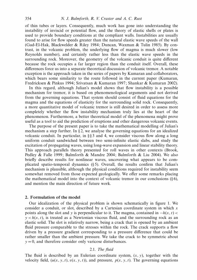
A key feature of (4.6) is that the second term, which arises from the deformationof the elastic wall, is stabilizing for large elastic wave speeds. However, as those wavespeeds decrease, the sign of this term switches (see figure 2), and the deformation ofthe wall also becomes destabilizing, implying that there is no threshold in Reynoldsnumber for long-wave instability. The conduit is then unstable even in the lubricationlimit. The critical elastic wave speed β is also shown in figure 2. The switch occurswhen an elastic wave speed approaches the speed with which disturbances propagatenaturally in the fluid (equal to three with the current non-dimensionalization). Morespecifically, the switch is at a Rayleigh wave speed of three, as described further in§ 4.4. This result is of the same flavour as that reported by Kumaran et al. (1994) forflow down a gel-walled tube.
4.2. Short (or nearly inviscid) waves
We derive short-wavelength estimates for the eigenvalue Λ of the boundary-layermodel as follows (cf. Chang et al. 1993). For k � 1 or R � 1, over the bulk of the

Instability in narrow elastic conduits 361
fluid the term ψ ′′′ in (4.2) is negligible, in which case,
(U − c)2d
dy
(ψ
U − c
)= −GD(k, Λ)
R, (4.8)
where c = −iΛ/k is the complex wave speed. We readily integrate:
ψ = −GD
R(U − c)
∫ y
0
dy
[U (y) − c]2≡ ψI , (4.9)
on imposing ψ(0) = ψ ′′(0) = 0. This solution cannot be made to satisfy the remainingboundary conditions, reflecting how a viscous sublayer arises near the wall. There, wemust reinstate ψ ′′′, to find the solution, ψ =ψI + ψB , with
ψB ∼ Be−ς(1−y), ς = (1 − i)
√kcR
2, (4.10)
where B is a constant of integration. Enforcing the boundary conditions (bearingin mind that cRψ ′
I = p +3RψI and ψ ′B = ςB at y = 1) now provides the dispersion
relation,
cR = GD
[1
3 − ςc+ c
∫ 1
0
dy
(U − c)2
](4.11)
cR =GD
3 − cς+
GD
2c − 3
[1 +
2c√3(2c − 3)
tan−1
√3
2c − 3
]. (4.12)
Note that the inviscid problem corresponds to taking the limit |ς | → ∞ with G/R
fixed in the formulae above and dropping ψB , in which case (4.12) is exact. Notably,in the inviscid limit, we can have c → 3/2 for the neutrally stable case and a criticallayer develops which we briefly discuss in § 4.4.
The dispersion relation (4.12) can be simplified further given that k � 1, althoughthe precise details depend upon the size of the elastic wave speeds. We present some ofthe details in Appendix A, and summarize the main results as follows. Let cr = Re(c)and Λr = Re(Λ). Then, for cr � β ,
cr ∼
√2kG
R
(1 − β2
α2
), Λr ∼ −k3/4. (4.13)
Alternatively, for cr ∼ β , the eigenvalues satisfy at leading order
DR(cr ) = D(k, −ikcr ) = 0. (4.14)
This is the dispersion relation for an elastic half-space bounded by an shear-freeinterface at fixed pressure. Consequently, the solutions are Rayleigh waves (Love 1944)with cr = cR . The Rayleigh waves occur as counter-propagating pairs (the symmetry-breaking due to the direction of fluid flow does not appear at leading order). TheRayleigh waves propagating backwards with respect to the fluid appear to be alwaysrelatively strongly damped, and we ignore them henceforth. At higher-order, theforward-propagating Rayleigh waves become modified by viscous dissipation in thefluid, and Λr ∼ −k−1/2.
These results imply that when the elastic wave speeds are large, there are twoscaling regimes (at fixed Reynolds number). First, for 1 � k1/2 � α, β , the growth rateplummets as −k3/4 (and the propagation speed increases as k1/2). When k1/2 ∼ α, β ,

362 N. J. Balmforth, R. V. Craster and A. C. Rust
however, the disturbances become Rayleigh-like waves and the growth rate turnsaround and approaches zero from below as −k−1/2. Overall, short waves are stable.
4.3. Slot-averaged theory
The simplest theory (3.10) predicts the dispersion relation,
9 − 3iΛ
k+ iR
(−12iΛ
5+
6k
5− Λ2
k
)= ikGD(k, Λ). (4.15)
The second, improved, theory (3.12) gives
9 − 3iΛ
k+ iR
(54k
35− 102iΛ
35− 6Λ2
5k
)= ikGD(k, Λ). (4.16)
We analyse the second of these for comparison with the earlier results. Marginalstability occurs for Λ = iω, with ω real. Thence, provided κα and κβ remain real,
ω = −3k, R =5kGαβ2
162√
α2 − 9
[4
αβ
√(α2 − 9)(β2 − 9) −
(9
β2− 2
)2]
. (4.17)
This is identical to the long-wave results of the boundary-layer model (though it isnot restricted to long waves). A similar calculation for the first slot-averaged modelgives a result in error by a factor of order unity, vindicating our improvement of thattheory.
For an infinite elastic wave speed, short waves have the limiting eigenvalues,
Re(Λ) ∼ − 5
4R, Im(Λ) ∼ −k3/2
√5G
3R
(1 − β2
α2
), (4.18)
and are therefore always stable. For finite α and β , on the other hand, short wavesonce again limit to Rayleigh waves with wave speed, cR . The damping or growth ofthese modes appears at order k−2, leading to
Re(Λ) ∼ 3(cR − 3)
kGD′R(cR)
, (4.19)
where DR(cr ) ≡ D(k, −ikcR)/k. As long as k1/2 � α, β , the growth rate therefore firstdecreases and flattens out to a minimum value near −5/4R. Once k1/2 ∼ α, β , thegrowth rate begins to increase back toward zero. Because D′
R(cR) < 0, the shortwaves are only stable if cR > 3. That is, if the Rayleigh waves are slower than fluiddisturbances, they are destabilized by the coupling with the fluid; faster waves arestable. These trends are illustrated below, and have some similarities with the resultsof the boundary-layer theory described earlier.
4.4. Numerical results
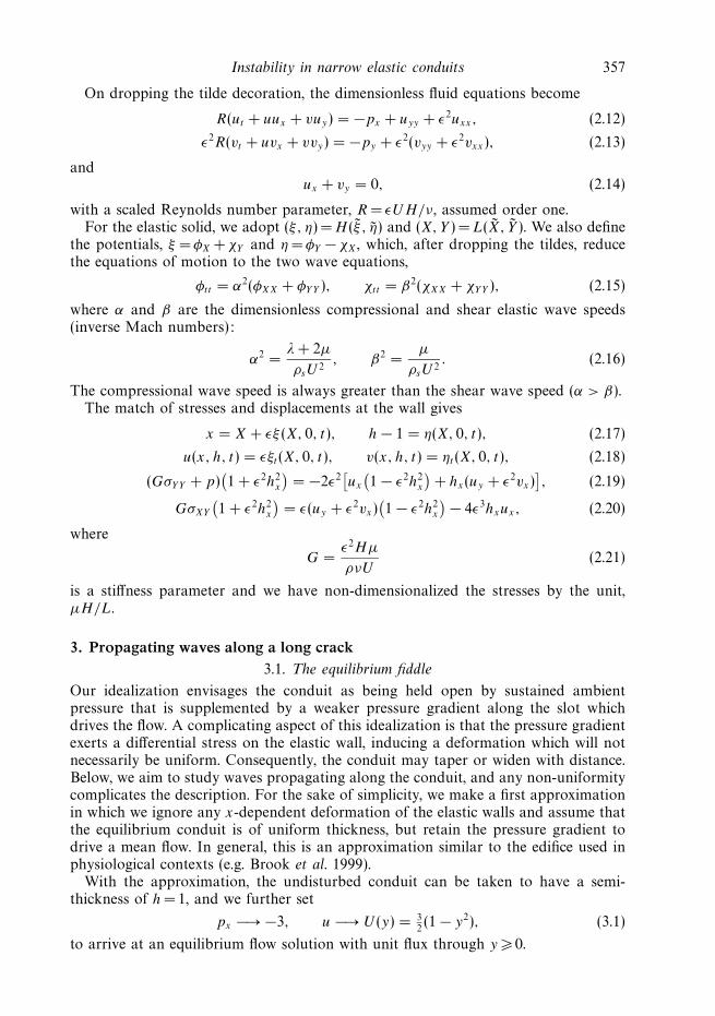
We summarize and extend the results above using numerical computations with thelinear boundary-layer model, as shown in figures 3–5. We take G = 2, in view ofthe secondary importance of this parameter to stability. Figure 3 shows growth ratesagainst k for an unstable flow with different elastic wave speeds (but with α/β = 2),and displays an instability with long-wave character. As elastic wave speed decreases,the band of unstable wavenumbers widens, and by β = 2, the unstable band extendsto rather higher wavenumber.
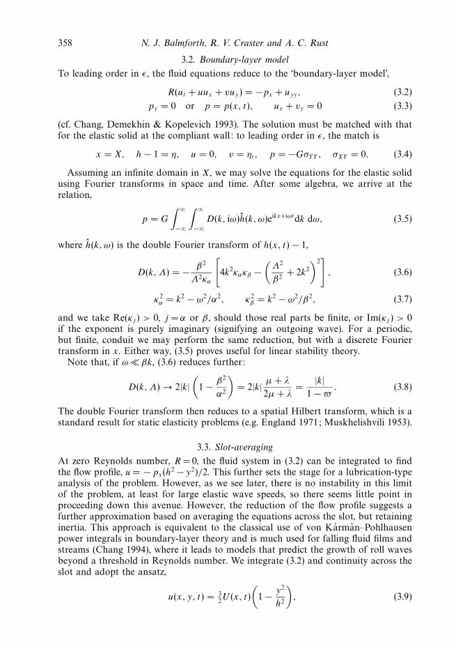
Figure 4 shows further details of the growth rates for low and high wavenumber,and compares the numerical results with the asymptotic predictions derived above and
Instability in narrow elastic conduits 363
0 10 20 30 40 50–4
–3
–2
–1
0
k
Gro
wth
rat
e
β = ∞
20
10
5
2
0 1 2 3 4–0.1
0
0.1
0.2
0.3
Figure 3. Sample growth rates against k for R =2 and G = 2, and for a variety of elasticwave speeds with α/β = 2 and β as indicated.
10–2 100 102
101
β = 20
10
5
2
3
4cR = 3
cr(k)
k
NumericalLeading order; RayleighHigher order
–25
–20
–15
–10
–5
0
20
β =10
10–2 10–1 100 101 102 103
–0.2
–0.1
0.1
0.2
0
5
β = 2
34
λr(k)
λr(k)
10–2 100
0
0.2
–0.2
∞β = ∞
Figure 4. Wave speeds and growth rates against k for R = 2 and G = 2, and for a variety ofelastic wave speeds with α/β = 2 and β as indicated. The numerical results are compared withthe asymptotic predictions for long and short waves, as given in Appendix A (for the β → ∞wave speed, a higher-order approximation than given in the Appendix is also included; theslight improvement did not merit the inclusion of the actual formulae).
in the Appendix. In particular, this figure highlights the switch over from long waves,with cr = 3 and Λr ∼ (6R/5)k2, to short Rayleigh-like waves with weak damping rates(except for the curve with β → ∞).
364 N. J. Balmforth, R. V. Craster and A. C. Rust
β = ∞ β = 20 β = 10 β = 5
β = 4
log10 R
log 1
0 k
0–1 1 2–1.0
–0.5
0
0.5
1.0
β = 3.25 β = 3 β = 2
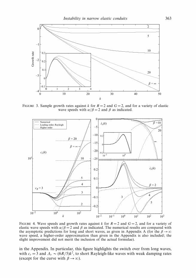
Figure 5. Growth rate shown as a density on the (log10 R, log10 k)-plane for the boundary-layermodel with β/α = 2 and G = 2. The dark dotted contours show positive growth rates and areseparated by increments of 0.025. The light dotted contours show negative growth rates spacedby 0.25 from 0 to −1, and then in intervals of unity for smaller values. The solid contourdisplays the stability boundary.
–3 –2 –1 0 1 2 3 4–2
–1
0
1
2
3
log10 R
log 1
0 k
3.25
3.5
3.2
3 2.75 2.5
β = 4, 5, 10, ∞
Stable
Unstable
R � k 5/3
R � k
R � k–1
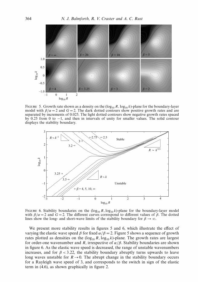
Figure 6. Stability boundaries on the (log10 R, log10 k)-plane for the boundary-layer modelwith β/α = 2 and G = 2. The different curves correspond to different values of β . The dottedlines show the long- and short-wave limits of the stability boundary for β → ∞.
We present more stability results in figures 5 and 6, which illustrate the effect ofvarying the elastic wave speed β for fixed α/β = 2. Figure 5 shows a sequence of growthrates plotted as densities on the (log10 R, log10 k)-plane. The growth rates are largestfor order-one wavenumber and R, irrespective of α/β . Stability boundaries are shownin figure 6. As the elastic wave speed is decreased, the range of unstable wavenumbersincreases, and for β < 3.22, the stability boundary abruptly turns upwards to leavelong waves unstable for R → 0. The abrupt change in the stability boundary occursfor a Rayleigh wave speed of 3, and corresponds to the switch in sign of the elasticterm in (4.6), as shown graphically in figure 2.

Instability in narrow elastic conduits 365
0 5 10 15 20 25 30 35 40 45 503. 5
3
2. 5
2
–1.5
–1.0
–0.5
0
k
Gro
wth
rat
e
10
β = 10
BLTSAM–1SAM–2
0 1 2 3–0.05
0
0.05
0.10
0.15
0.20
0.25
∞
∞
Figure 7. A comparison between the results of the boundary-layer theory (BLT) and theslot-averaged models (SAM). Shown are growth rates against k for R = 2, G = 2, α/β =2 andβ = 10 and ∞.
log10 R
log 1
0 k
–1 0 1 2–1
0
1
β = ∞ β = 5 β = 3
Figure 8. Growth rates shown as density on the (log10 R, log10 k)-plane for the improved slot-averaged model (3.12) with α =2β , G = 2 and β = ∞, 5 and 3. The contours have the samelevels as in figure 5.
For large R, the stability boundary has the dependence, R ∼ k17/11, whereas atsmaller R, we find either R ∼ k or R ∼ k−1, depending on whether β is above orbelow 3.22, respectively. The curious dependence, R ∼ k17/11, can be verified fromshort-wave theory along the lines sketched out above, but also adding the next termin the solution for ψI . This turns out to be necessary since c → 3/2 on this partof the boundary, indicating that the neutrally stable inviscid solution (|ς | → ∞) candevelop singularities along the midline of the conduit (where the wave speed matchesthe maximum flowspeed, i.e. the inviscid solution develops a critical layer). The third(short-wave, low β) part of the stability boundary, R ∼ k−1, corresponds to neutralRayleigh waves with c → cR , for which there is no pressure perturbation at the wall,only a displacement (and kR arises as the eigenvalue of (4.2)).
Figure 7 displays a comparison between the results of the boundary-layer modeland the two slot-averaged models presented earlier. Both averaged theories capturethe long-wave instability, although the improved model compares better with theboundary-layer theory, as shown further in figure 8, which should be compared

366 N. J. Balmforth, R. V. Craster and A. C. Rust
0 50 100 150 200
0.1
0
250 300 350 400 450
10–1
10–2
10–3
10–4
10–5
10–6
Time, t
�h2 �
and
�U
2 ��U2�
�h2�
x –
5t/2
h(x,t)
50 100 150 200 250 300 350 400 450
1
2
3
4
5
6
h(x,t)U(x,t)
(a)
(b) (c) (d)
0.2
0
Figure 9. A numerical solution of the slot-averaged model (3.12) for R = 1.5, β/α = 1/2 (withβ → ∞) and G = 2. (a) The averages of (5.2). The inset shows h(x, t) as a density on the (t, x)-plane. (b)–(d) show further details of the solution. (b) A phase portrait on the (〈h2〉, 〈U 2〉)-plane.(c) Time series at two fixed positions. (d) Four snapshots of the solutions near the end of thecomputation.
with the relevant panels of figure 5. The comparison is less favourable at higherwavenumbers, where the growth rates are predicted to flatten out for the averagedtheories whereas the actual damping rates of the boundary-layer model are stronger.Note that boundary-layer theory is strictly valid for small εk, and the highwavenumbers computed in the figures do not necessarily conform to this condition.The computations might then best be thought of as a test of the slot-averagedtheories, which are essentially approximations of the boundary-layer model.
5. Nonlinear wavesTo catch a glimpse of the nonlinear dynamics of unstable propagating waves, we
solve the improved slot-averaged model (3.12) numerically in a periodic domain oflength 2π. We adopt the simplifying assumption (ω/k) � α, β , and use a Fouriertransform to compute the pressure in terms of the displacement of the wall:
h = 1 +
∞∑n=−∞
hn einx, p = 2iG(1 − β2α2)
∞∑n=−∞
n2hn einx sgn(n). (5.1)
The PDEs are then solved using a standard implicit time integrator after dealing withspatial derivatives with either a finite-difference or a pseudo-spectral scheme. Initial
Instability in narrow elastic conduits 367
0 50 100 150 200 250 300 350 400 450
10–1
10–3
10–2
10–4
10–5
10–6
Time, t
�U2�
�h2�
50 100 150 200 250 300 350 400 450
1
2
3
4
5
6
h(x,t)U(x,t)
�h2 �
and
�U
2 �
x –
5t/2
(a)
(b) (c) (d)
0.1
0
0.2
0
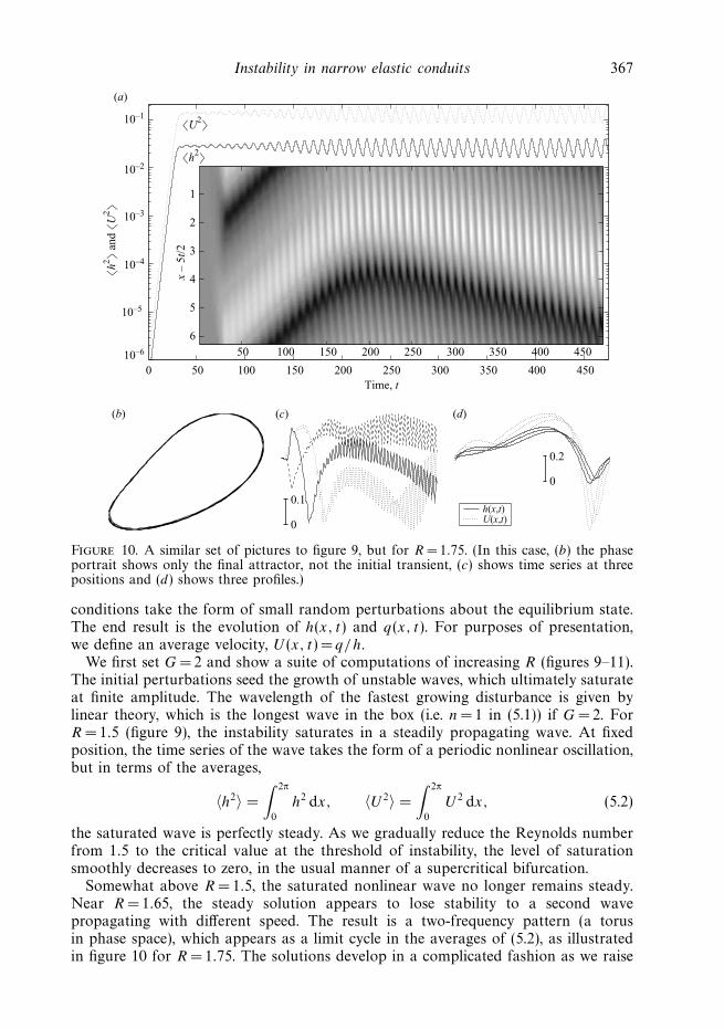
Figure 10. A similar set of pictures to figure 9, but for R = 1.75. (In this case, (b) the phaseportrait shows only the final attractor, not the initial transient, (c) shows time series at threepositions and (d) shows three profiles.)
conditions take the form of small random perturbations about the equilibrium state.The end result is the evolution of h(x, t) and q(x, t). For purposes of presentation,we define an average velocity, U (x, t) = q/h.
We first set G = 2 and show a suite of computations of increasing R (figures 9–11).The initial perturbations seed the growth of unstable waves, which ultimately saturateat finite amplitude. The wavelength of the fastest growing disturbance is given bylinear theory, which is the longest wave in the box (i.e. n= 1 in (5.1)) if G =2. ForR = 1.5 (figure 9), the instability saturates in a steadily propagating wave. At fixedposition, the time series of the wave takes the form of a periodic nonlinear oscillation,but in terms of the averages,
〈h2〉 =
∫ 2π
0
h2 dx, 〈U 2〉 =
∫ 2π
0
U 2 dx, (5.2)
the saturated wave is perfectly steady. As we gradually reduce the Reynolds numberfrom 1.5 to the critical value at the threshold of instability, the level of saturationsmoothly decreases to zero, in the usual manner of a supercritical bifurcation.
Somewhat above R =1.5, the saturated nonlinear wave no longer remains steady.Near R = 1.65, the steady solution appears to lose stability to a second wavepropagating with different speed. The result is a two-frequency pattern (a torusin phase space), which appears as a limit cycle in the averages of (5.2), as illustratedin figure 10 for R = 1.75. The solutions develop in a complicated fashion as we raise
368 N. J. Balmforth, R. V. Craster and A. C. Rust
0 100 200 300 400 500 600 700 800 900Time, t
100 200 300 400 500 600 700 800 900
1
2
3
4
5
6
h(x,t)U(x,t)
10–1
10–2
10–3
10–4
10–5
10–6
�h2 �
and
�U
2 ��U2�
�h2�
x –
5t/2
(a)
(b) (c) (d)
0.1
0
0.2
0
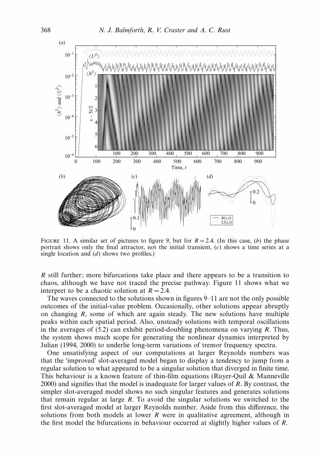
Figure 11. A similar set of pictures to figure 9, but for R = 2.4. (In this case, (b) the phaseportrait shows only the final attractor, not the initial transient, (c) shows a time series at asingle location and (d) shows two profiles.)
R still further; more bifurcations take place and there appears to be a transition tochaos, although we have not traced the precise pathway. Figure 11 shows what weinterpret to be a chaotic solution at R = 2.4.
The waves connected to the solutions shown in figures 9–11 are not the only possibleoutcomes of the initial-value problem. Occasionally, other solutions appear abruptlyon changing R, some of which are again steady. The new solutions have multiplepeaks within each spatial period. Also, unsteady solutions with temporal oscillationsin the averages of (5.2) can exhibit period-doubling phenomena on varying R. Thus,the system shows much scope for generating the nonlinear dynamics interpreted byJulian (1994, 2000) to underlie long-term variations of tremor frequency spectra.
One unsatisfying aspect of our computations at larger Reynolds numbers wasthat the ‘improved’ slot-averaged model began to display a tendency to jump from aregular solution to what appeared to be a singular solution that diverged in finite time.This behaviour is a known feature of thin-film equations (Ruyer-Quil & Manneville2000) and signifies that the model is inadequate for larger values of R. By contrast, thesimpler slot-averaged model shows no such singular features and generates solutionsthat remain regular at large R. To avoid the singular solutions we switched to thefirst slot-averaged model at larger Reynolds number. Aside from this difference, thesolutions from both models at lower R were in qualitative agreement, although inthe first model the bifurcations in behaviour occurred at slightly higher values of R.
Instability in narrow elastic conduits 369
0 10 20 30 40 50Time, t
�U2�/3
�h2�
5 10 15 20 25 30 35 40 45 50 55
1
2
3
4
5
6
h(x,t)U(x,t)
10–1
10–2
10–3
10–4
10–5
�h2 �
and
�U
2 �
(a)
(c)(b)
x –
3t
0.5
0
0.2
0
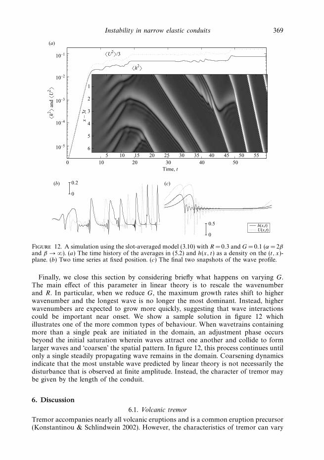
Figure 12. A simulation using the slot-averaged model (3.10) with R = 0.3 and G =0.1 (α = 2βand β → ∞). (a) The time history of the averages in (5.2) and h(x, t) as a density on the (t, x)-plane. (b) Two time series at fixed position. (c) The final two snapshots of the wave profile.
Finally, we close this section by considering briefly what happens on varying G.The main effect of this parameter in linear theory is to rescale the wavenumberand R. In particular, when we reduce G, the maximum growth rates shift to higherwavenumber and the longest wave is no longer the most dominant. Instead, higherwavenumbers are expected to grow more quickly, suggesting that wave interactionscould be important near onset. We show a sample solution in figure 12 whichillustrates one of the more common types of behaviour. When wavetrains containingmore than a single peak are initiated in the domain, an adjustment phase occursbeyond the initial saturation wherein waves attract one another and collide to formlarger waves and ‘coarsen’ the spatial pattern. In figure 12, this process continues untilonly a single steadily propagating wave remains in the domain. Coarsening dynamicsindicate that the most unstable wave predicted by linear theory is not necessarily thedisturbance that is observed at finite amplitude. Instead, the character of tremor maybe given by the length of the conduit.
6. Discussion6.1. Volcanic tremor
Tremor accompanies nearly all volcanic eruptions and is a common eruption precursor(Konstantinou & Schlindwein 2002). However, the characteristics of tremor can vary

370 N. J. Balmforth, R. V. Craster and A. C. Rust
considerably. The signal may originate from as deep as 40 km below ground level,or as shallow as a few hundred metres (Aki & Koyanagi 1981). It can have agradual or abrupt onset, be harmonic or anharmonic, and last minutes, days ormonths (Konstantinou & Schlindwein 2002). Typically, the signal comes from lessthan 10 km depth, and the frequency spectra display a distribution of sharp peaksconcentrated between 0.1–7 Hz. There can be systematic changes in tremor duringeruptions including what appear to be period doublings and halvings.
Given the range of tremor properties, depths of origin and association with allstyles of eruptions (explosive, effusive; magmatic, phreatic; passive degassing), theremay be multiple origins of volcanic tremor. Several mechanisms for tremor generationhave been proposed including bubble growth or collapse, jerky crack propagation,oscillations of magma chambers, resonance of fluid-filled cracks and flow-inducedoscillations of conduits (Julian 1994; Konstantinou & Schlindwein 2002). Modelsinvolving resonance require a disturbance to trigger oscillations and while there aremany plausible sources of so-called ‘long-period’ events, which decay after secondsor tens of seconds, tremor requires a disturbance that is sustained for minutes oreven months. Sustained resonance could be caused by continued formation of shockwaves (Morrissey & Chouet 2001) or gas slugs (Cruz & Chouet 1997; James et al.2004), however, these seem to require special circumstances and do not explain tremorduring volcanic eruptions of all styles and compositions. By contrast, flow-inducedoscillations in the conduit walls could provide a source of sustained seismicity, lastingas long as flow continued at a sufficient speed. Moreover, although the sample resultspresented by Julian involve very high fluid velocities (45–110 m s−1) and frequenciesat the high end of tremor (∼5 Hz), his model can explain the apparent nonlinearphenomena observed at several volcanoes (Julian 2000; Konstantinou 2002).
The theory we have presented amplifies further on Julian’s mechanism: a linearstability analysis indicates that flow-induced oscillations can appear at arbitrarily low(but non-zero) Reynolds numbers. Furthermore, the stability of the system dependson the crack aspect ratio, fluid speed and elastic wave speeds. However, up to thispoint we have not considered the physical parameters relevant to volcanic tremor. Tothis end, we return to dimensional units (restoring the tildes to decorate dimensionlessvariables) and record the dimensionless critical wavenumber, kcr , below which thesystem is unstable to long waves. From (4.7), with k ∼ 1 (which corresponds to wavesof wavelength comparable to the length of the crack), we find
1 ∼ R
G=
ρU 2
ρsεβ2or U ∼
(ερs
ρ
)1/2
β, (6.1)
where β is the true dimensional shear wave speed. Evidently, stability does not dependdirectly on viscosity, but the more viscous the fluid, the greater the pressure gradientrequired to drive flow at a given velocity through a crack with a given thickness.
The estimate in (6.1) is actually quite natural for our conduit, and can be arrived atmore directly with dimensional analysis. The destabilizing inertial terms, ρ(ut + uux),are order ρU 2/L. These are opposed by the pressure gradient, px ∼ p/L, arising fromthe elastic stresses due to the deformation of the wall. Since the elastic displacementsare order H , we see immediately from the constitutive relation that p ∼ µH/L. Thebalance of pressure gradient and inertia then gives (6.1).
To assess the feasibility of our model for generating volcanic tremor we considerε = 10−4 and β = 2 km s−1, which are towards the low end of physically possibleparameters. The estimate in (6.1) then suggests that flow speeds of tens of metresper second are required for instability. Figure 13 shows a more refined calculation
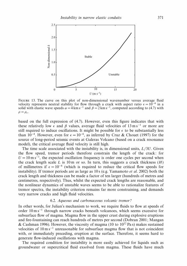
Instability in narrow elastic conduits 371
5 10 15 200
0.5
1.0
1.5
2.0
2.5
U (m s–1)
Non
-dim
ensi
onal
k
Unstable
Stable
Figure 13. The curve on this plot of non-dimensional wavenumber versus average fluidvelocity represents neutral stability for flow through a crack with aspect ratio ε = 10−4 in asolid with elastic wave speeds α = 4 km s−1 and β = 2 km s−1, computed according to (4.7) withρ = ρs .
based on the full expression of (4.7). However, even this figure indicates that withthese relatively low ε and β values, average fluid velocities of 13 m s−1 or more arestill required to induce oscillations. It might be possible for ε to be substantially lessthan 10−4. However, even for ε = 10−6, as inferred by Cruz & Chouet (1997) for thesource of long-period seismic events at Galeras Volcano (based on a crack resonancemodel), the critical average fluid velocity is still high.
The time scale associated with the instability is, in dimensional units, L/3U . Giventhe flow speed, tremor periods therefore constrain the length of the crack: forU = 10 m s−1, the expected oscillation frequency is order one cycles per second whenthe crack length scale L is 10 m or so. In turn, this suggests a crack thickness (H )of millimetres if ε = 10−4 (which is required to reduce the critical flow speeds forinstability). If tremor periods are as large as 10 s (e.g. Yamamoto et al. 2002) both thecrack length and thickness can be made a factor of ten larger (hundreds of metres andcentimetres, respectively). Thus, whilst the expected crack lengths are reasonable, andthe nonlinear dynamics of unstable waves seems to be able to rationalize features oftremor spectra, the instability criterion remains far more constraining, and demandsvery narrow cracks and high fluid velocities.
6.2. Aqueous and carbonaceous volcanic tremor?
In other words, for Julian’s mechanism to work, we require fluids to flow at speeds oforder 10 m s−1 through narrow cracks beneath volcanoes, which seems excessive forsubsurface flow of magma. Magma flow in the upper crust during explosive eruptionsand fire-fountaining can reach hundreds of metres per second (Dobran 2001; Mangan& Cashman 1996). However, the viscosity of magma (10 to 1012 Pa s) makes sustainedvelocities of 10 m s−1 unreasonable for subsurface magma flow that is not coincidentwith, or immediately preceding, eruption at the surface. Therefore, it seems hard togenerate flow-induced oscillations with magma.
The required condition for instability is more easily achieved for liquids such asgroundwater or supercritical fluid exsolved from magma. These fluids have much
372 N. J. Balmforth, R. V. Craster and A. C. Rust
lower viscosity than magma, allowing higher flow speeds, and do not have a largedensity contrast with rock (so ρ/ρs is not overly small). In fact, aqueous fluids arepresent at all volcanoes and eruptions of magma are typically preceded by increasedgas emissions indicative of subsurface flow. Furthermore, if a low viscosity fluid isrequired for deep tremor, this could explain the general lack of long period seismicityin recharge zones beneath intermediate and silicic volcanoes where there is magmamovement but the magma is not saturated in volatiles. However, this also begs thequestion of whether we could expect to find high-speed flow of aqueous fluid at thedepths required to explain tremor.
To what depths are aqueous fluids present? There is growing evidence that magmasa few kilometers below volcanoes are often saturated in volatiles (mixtures of H2O,CO2, etc.; Wallace 2001), and consequently a free, low-viscosity fluid is expected atsuch levels. However, volatile solubility increases with depth, suggesting that thereshould be no free aqueous fluid below 10 km. Yet the deepest reported tremororiginated about 40 km below Kilauea Volcano (Aki & Koyanagi 1980). Nevertheless,magmas can be saturated in volatiles at depths in excess of 10 km if there is sufficientCO2 in the melt (e.g. Lowenstern 2001), and Gerlach et al. (2002) have calculatedthat a low viscosity fluid could exsolve about 30 km under Kilauea. Though stillshallower than Aki & Koyanagi deepest tremor, this opens up the possibility thata carbonaceous fluid played a role in generating those deep sustained vibrations. Infact, substantial crystallization of stalled magma could lead to CO2 saturation andfluid exsolution even at 40 km depth.
Volatile-rich fluids can also be generated at great depths by dehydration metamor-phism of subducted oceanic crust. Tremor has recently been detected in the mantleat two subduction zones at depths where the down-going slab is expected to reachhigh enough temperatures for water release (Obara 2002; Rogers & Dragert 2003).The generation of tremor in the portion of the mantle where one would expect aseparate water phase is consistent with a mechanism based on the flow of low viscosityfluids.
We conclude that although magma transport is unlikely to generate flow-inducedoscillations, rapid flow of H2O- or CO2-rich fluids is a possible source for tremor(a) in the upper several kilometers of crust where aqueous fluids are present,(b) at greater depth where the magma has high CO2 content, and (c) in the mantleabove dehydrating subducted crust. Moreover, the same mechanism could produce‘long-period’ events if the fluid only intermittingly achieves sufficient speed to inducewall oscillations. Note that a relatively dense fluid phase is essential, otherwise the den-sity contrast with rock does not favour instability, which precludes a mechanism basedon vapour flow.
6.3. Conclusions
Our stability analysis indicates that some fluids, conduit geometries and eruptionstyles are more likely to cause tremor by flow-induced oscillations than others. Inparticular, we have found that narrow conduits and high fluid speeds tend to generateflow-induced tremor. Also, as we argue in Appendix B, planar conduits seem far moreunstable than tube-like fluid conduits. Except for shallow seismicity during explosiveor fountaining activity, maintaining sufficient fluid speeds (>10 m s−1) by realisticpressure gradients to induce oscillations requires sustained flow of low-viscosityaqueous or carbonaceous fluid rather than magma. These conclusions are consistentwith observations by McNutt (2002) in a study of tremor from 50 eruptions at 31volcanoes comparing tremor characteristics and corresponding eruption parameters.

Instability in narrow elastic conduits 373
McNutt lists four trends in the data:
1) large eruptions produce stronger tremor than small ones;2) fissure eruptions produce stronger tremor than circular vents for the same
fountain height;3) eruptions with higher gas content produce stronger tremor than those with low
gas content at the same volcano; and4) phreatic eruptions [eruptions that eject broken rock and vapour but no magma]
produce stronger tremor than magmatic eruptions [eruptions that do eject magma] forthe same VEI [Volcanic Explosivity Index, a measure of the magnitude and intensity ofan eruption].’
Much remains to be done. First, and foremost, is to change the conduit geometry:an arguably more plausible configuration involves a relatively short conduit, boundedby fluid reservoirs at either end. In this latter case, flow instability arises when the wallsrock back and forth in near unison, and the mathematical description invokes normalmodes rather than waves. A key physical issue that must be addressed is whetherthe flushing action of the flow down the finite conduit can suppress instability (theperiodic boundaries we have considered here allow waves to re-enter the conduit andcontinue to grow).
For the volcanic application, we must further develop the comparison with observa-tions. The sole observations used here were the rough characteristics of tremor and thegeological conditions. However, there are detailed seismic studies of tremor sourcesand decomposition of the outgoing elastic wavefield, both of which should be takeninto consideration in testing the theoretical model. We note that the flow instabilitygenerates roughly equal amounts of shear-wave and compressional-wave radiation(χ ∼ φ), and that the seismic signature may be similar to that already explored inacoustic resonance models for tremor (Chouet 2003, and references therein).
N. J. B. thanks Susan Schwartz for bringing this problem to his attention. Thiswork began at the 2003 GFD Summer Study Program, Woods Hole OceanographicInstitution (which is supported by NSF and ONR). We thank the participantsfor discussions. We also thank two anonymous reviewers and K. Cashman andD. Villagomez for their comments. N. J. B. was supported by the National ScienceFoundation (Grant no. DMS 72521).
Appendix A. Short-wave resultsIn this Appendix, we present some of the details of the short-wave stability theory
of the boundary-layer model. First, consider the limit β → ∞, with α/β held fixed.Then, D ∼ 2k(1 − β2/α2). Thus, considering k � 1, we find
c ∼
√2kG
R
(1 − β2
α2
). (A 1)
The first imaginary correction to c appears at order k−1/4:
Im(c) ∼ −1
2
[G(1 − β2/α2)
2kR3
]1/4
or Re(Λ) ∼ −1
2
[k3G(1 − β2/α2)
2R3
]1/4
. (A 2)

374 N. J. Balmforth, R. V. Craster and A. C. Rust
Secondly, let β and α remain order one for k � 1. Then, if c remains order unity(specifically order β),
D(k, −ikc) → kαβ2
c2√
α2 − c2
[4
αβ
√(α2 − c2)(β2 − c2) −
(2 − c2
β2
)2]
≡ kDR(c). (A 3)
The dispersion relation becomes
cR(3 − cς)
kG
{1 +
(3 − cς)
(2c − 3)
[1 +
2c√3(2c − 3)
tan−1
√3
2c − 3
]}−1
= DR(c), (A 4)
and so the leading-order eigenvalues correspond to zeros of DR(cr ), which gives theRayleigh waves. The imaginary correction to the Rayleigh wave speed, cR (which isof order β), appears at higher order. Provided cR > 3/2, the growth rate follows from
Λr =(2cR − 3)2
GD′R(cR)
√R
2k|cR|
[1 +
2cR√3(2cR − 3)
tan−1
√3
(2cR − 3)
]−2
. (A 5)
If α and β are relatively large (though not as large as k), the Rayleigh wave speed isalso large, and we make further approximations to arrive at
Re(Λ) ∼ |cR|3/2GD′
R(cR)
√R
2k. (A 6)
If β < 2, the Rayleigh wave speed can become smaller than 3/2 and a different scalingof growth rate then results. We ignore this possibility here.
Appendix B. The cylindrical conduitMagma mostly rises through the Earth’s brittle crust through fractures forming
sheets of magma. Lava sometimes erupts from linear fissures. However, flow isusually localized by cooling, producing a cylindrical form at the top of the conduit.We now briefly assess the feasibility of flow through a cylindrical conduit generatingtremor.
We consider a fluid-filled tube of length L and radius H in an elastic solid. Thecylindrical coordinate system (r, θ, z) is set so that the z-axis is in the centre ofthe tube and the solid–fluid interface is at r =h(z, t). Flow is two-dimensional withvelocity field (v, 0, w).
We non-dimensionalize as for the planar conduit, with x and y replaced with z and r ,respectively. The non-dimensional boundary-layer equations are
R(wt + wwz + vwr ) = −pz +1
r(rwr )r , pr = 0, (B 1)
and
wz +1
r(rv)r = 0. (B 2)
We content ourselves with a discussion of the linear problem using a slot-averagedapproximation. We take the velocity of the fluid to be
w(r, z, t) = 2W (z, t)
(1 − r2
h2
), (B 3)

Instability in narrow elastic conduits 375
so that the tube-averaged velocity is W (z, t) and the profile is parabolic. The radialintegrals of (B 1) and (B 2) then lead to the system,
R(h2W )t + 43R(h2W 2)z = −h2pz − 8W, (h2)t + (h2W )z = 0. (B 4)
These equations support an equilibrium flow with W = 1, h = 1 and pz = −8.A short diversion into solving the elasticity equations in cylindrical geometry with
a Fourier transform in z (with or without acceleration terms, and using the propertiesof Bessel functions) yields the leading-order matching condition,
p =2G
ε[h(x, t) − 1]. (B 5)
(The dimensionless radial polar coordinates for the elastic solid must be taken to be(R, Θ, Z), with R ∈ [ε, ∞), and expansion for small ε eventually yields (B 5).)
Linear stability analysis about the equilibrium leads to the dispersion relation,
2ikR
(4
3+
8Λ
3ik− Λ2
k2
)+ 16
(2 +
Λ
ik
)=
2ikG
ε, (B 6)
and it is straightforward to show that waves are always stable.A similar negative result can be obtained from a long-wave expansion of the
boundary-layer model in (B 1)–(B 2). In that case, we can establish that, if the modelis unstable, then the critical Reynolds number must be of order G/εk. This criticalcondition can be written in the alternative form, U ∼ β(ρs/ρk)1/2 where β is thedimensional elastic shear wave speed. By contrast, the equivalent condition for theplanar conduit is U ∼ β(εkρs/ρ)1/2. Thus, for wavelengths of order of the crack length(k = 1), the flow speed required for instability in the cylindrical conduit is much higherthan in the planar conduit by a factor of order ε−1/2, and must exceed the elasticwave speeds.
These results are striking in view of known results for instability in flow throughelastic tubes (i.e. the physiological problem; Pedley 1980), which occurs at finiteReynolds number. One difference is that physiological models often use empiricallaws for the pressure and drag inside the tube. However, Kumaran’s (1995) resultsalso suggest that instability arises once flow speed exceeds a critical value, or if theelastic wave speed is reduced below a threshold, which is consistent with the resultsabove if those critical elastic wave speeds are slower than the flow speed.
REFERENCES
Aki, K. & Koyanagi, R. 1981 Deep volcanic tremor and magma ascent mechanism under Kilauea,Hawaii. J. Geophys. Res. 86, 7095–7109.
Balmforth, N. J. & Liu, J. 2004 Roll waves in mud. J. Fluid Mech. 519, 33–54.
Balmforth, N. J. & Mandre, S. 2004 Dynamics of roll waves. J. Fluid Mech. 514, 1–33.
Benjamin, T. B. 1960 Effects of a flexible boundary on hydrodynamic stability. J. Fluid Mech. 9,513–532.
Benjamin, T. B. 1963 The threefold classification for unstable disturbances in flexible surfacesbounding inviscid flows. J. Fluid Mech. 16, 436–450.
Brook, B. S., Pedley, T. J. & Falle, S. A. 1999 Numerical solutions for unsteady gravity-drivenflows in collapsible tubes: evolution and roll-wave instability of a steady state. J. Fluid Mech.396, 223–256.
Chang, H.-C. 1994 Wave evolution on a falling fluid film. Annu. Rev. Fluid Mech. 26, 103–136.
Chang, H.-C., Demekhin, E. A. & Kopelevich, D. I. 1993 Nonlinear evolution of waves on avertically falling film. J. Fluid Mech. 250, 433–480.
Chouet, B. 2003 Volcano seismology. Pure Appl. Geophys. 160, 739–788.
376 N. J. Balmforth, R. V. Craster and A. C. Rust
Cruz, F. G. & Chouet, B. A. 1997 Long-period events, the most characteristic seismicityaccompanying the emplacement and extrusion of a lava dome in Galeras Volcano, Colombia,in 1991. J. Volcanol. Geotherm. Res. 77, 121–158.
Dobran, F. 2001 Volcanic Processes: Mechanisms in Material Transport . Kluwer.
Duncan, J. H., Waxman, A. M. & Tulin, M. P. 1985 The dynamics of waves at the interfacebetween a viscoelastic coating and a fluid flow. J. Fluid Mech. 158, 177–197.
England, A. H. 1971 Complex Variable Methods in Elasticity . Wiley-Interscience.
Gad-El-Hak, M., Blackwelder, R. F. & Riley, J. J. 1984 On the interaction of compliant coatingswith boundary-layer flows. J. Fluid Mech. 140, 257–280.
Gerlach, T. M., McGee, K. A., Elias, T., Sutton, A. J. & Doukas, M. P. 2002 Carbon dioxideemission rate of Kilauea Volcano: implications for primary magma and the summit reservoir.J. Geophys. Res. 107, ECV3, 1–15.
Hagerty, M. T., Schwartz, S. Y., Garces, M. A. & Protti, M. 2000 Analysis of seismic andacoustic observations at Arenal volcano, Costa Rica, 1995–1997. J. Volcanol. Geotherm. Res.101, 27–65.
James, M. R., Lane, S. J., Chouet, B. & Gilbert, J. S. 2004 Pressure changes associated with theascent and bursting of gas slugs in liquid-filled vertical and inclined conduits. J. Volcanol.Geotherm. Res. 129, 61–82.
Julian, B. R. 1994 Volcanic tremor: nonlinear excitation by fluid flow. J. Geophys. Res. 99, 11 859–11 877.
Julian, B. R. 2000 Period doubling and other nonlinear phenomena in volcanic earthquakes andtremor. J. Volcanol. Geotherm. Res. 101, 19–26.
Konstantinou, K. I. 2002 Deterministic non-linear source processes of volcanic tremor signalsaccompanying the 1996 Vatnajkull eruption, central Iceland. Geophys. J. Intl 148, 663–675.
Konstantinou, K. I. & Schlindwein, V. 2002 Nature, wavefield properties and source mechanismof volcanic tremor: a review. J. Volcanol. Geotherm. Res. 119, 161–187.
Kumaran, V. 1995 Stability of the viscous flow of a fluid through a flexible tube. J. Fluid Mech.294, 259–281.
Kumaran, V., Fredrickson, G. H. & Pincus, P. 1994 Flow induced instability of the interfacebetween a fluid and a gel at low Reynolds number. J. Phys. Paris II 4, 893–911.
Landahl, M. 1962 On the stability of a laminar incompressible boundary layer over a flexiblesurface. J. Fluid Mech. 13, 607–632.
LaRose, P. G. & Grotberg, J. B. 1997 Flutter and long-wave instabilities in compliant channelsconveying developing flows. J. Fluid Mech. 331, 37–58.
Love, A. E. 1944 Treatise on the Mathematical Theory of Elasticity . 4th edn. Dover.
Lowenstern, J. B. 2001 Carbon dioxide in magmas and implications for hydrothermal systems.Mineralium Deposita 36, 490–502.
McNutt, S. R. 2002 Volcanic tremor and its use in estimating eruption parameters. EOS Trans.Am. Geophys. Un., Fall Meeting Suppl. 83, F1500–F1501.
Mangan, M. T. & Cashman, K. V. 1996 The structure of basaltic scoria and reticulite and inferencesfor vesiculation, foam formation, and fragmentation in lava fountains. J. Volcanol. Geotherm.Res. 73, 1–18.
Moriarty, J. A. & Grotberg, J. B. 1999 Flow-induced instabilities of a serous–mucus bilayer.J. Fluid Mech. 397, 1–32.
Morrissey, M. M. & Chouet, B. A. 2001 Trends in long-period seismicity related to magmaticfluid compositions. J. Volcanol. Geotherm. Res. 108, 265–281.
Muralikrishnan, R. & Kumaran, V. 2002 Experimental study of the instability of the viscous flowpast a flexible surface. Phys. Fluids 12, 775–780.
Muskhelishvili, N. I. 1953 Some Basic Problems of Elasticity . Noordhoff.
Obara, K. 2002 Nonvolcanic deep tremor associated with subduction in southwest Japan. Science296, 1679–1681.
Pedley, T. J. 1980 Fluid Mechanics of Large Blood Vessels . Cambridge University Press.
Rogers, G. & Dragert, H. 2003 Episodic tremor and slip on the cascadia subduction zone; thechatter silent slip. Science 300, 1942–1943.
Ruyer-Quil, C. & Manneville, P. 2000 Improved modelling of flows down inclined planes. Eur.Phys. J. B Fluids 15, 357–369.
Instability in narrow elastic conduits 377
Ryan, M. P. 1987 Neutral boyancy and the mechanical evolution of magmatic systems. In B. O.Mysen (ed.) Magmatic Processes: Physiochemical Principles. Spec. Publ. Geochem. Soc. 1,259–287.
Shankar, V. & Kumaran, V. 2002 Stability of wall modes in fluid flow past a flexible surface.Phys. Fluids 12, 2324–2338.
Srivatsan, L. & Kumaran, V. 1997 Stability of the interface between a fluid and a gel. J. Phys.Paris II 7, 947–963.
Wallace, P. J. 2001 Volcanic SO2 emissions and the abundance and distribution of exsolved gas inmagma bodies. J. Volcanol. Geotherm. Res. 108, 85–106.
Yamamoto, M., Kawakatsu, H., Yomogida, K. & Koyama, J. 2002 Long-period (12 sec) volcanictremor observed at Usu 2000 eruption; seismological detection of a deep magma plumbingsystem. Geophys. Res. Lett. 29, art. 1329.


