NBER WORKING PAPER SERIES

INSIDE THE BLACK BOX OF DOCTORAL EDUCATION:WHAT PROGRAM CHARACTERISTICS INFLUENCE

DOCTORAL STUDENTS’ ATTRITIONAND GRADUATION PROBABILITIES?

Ronald G. EhrenbergGeorge H. Jakubson

Jeffrey GroenEric So

Joseph Price

Working Paper 12065http://www.nber.org/papers/w12065

NATIONAL BUREAU OF ECONOMIC RESEARCH1050 Massachusetts Avenue

Cambridge, MA 02138February 2006

Ehrenberg is the Irving M. Ives Professor of Industrial and Labor Relations and Economics at CornellUniversity, Director of the Cornell Higher Education Research Institute (CHERI) and a research associateat the NBER. Jakubson is an associate professor of labor economics at Cornell University and a facultyassociate at CHERI. Groen is a research economist at the U.S. Bureau of Labor Statistics and a facultyassociate at CHERI. So and Price are both PhD students in economics at Cornell and graduate researchassistants at CHERI. We are grateful to Susan Dynarski, Alan Krueger, Michael McPherson, and conferenceparticipants at the Econometric Society Meetings for useful comments. Our research was funded by a grantfrom the Andrew W. Mellon Foundation and we are grateful to the Foundation for its support. The viewsexpressed herein are those of the author(s) and do not necessarily reflect the views of the Andrew W. MellonFoundation, the U.S. Bureau of Labor Statistics, or the National Bureau of Economic Research.

©2006 by Ronald G. Ehrenberg, George H. Jakubson, Jeffrey Groen, Eric So, and Joseph Price. All rightsreserved. Short sections of text, not to exceed two paragraphs, may be quoted without explicit permissionprovided that full credit, including © notice, is given to the source.

Inside the Black Box of Doctoral Education: What Program Characteristics Influence DoctoralStudents’ Attrition and Graduation Probabilities?Ronald G. Ehrenberg, George H. Jakubson, Jeffrey Groen, Eric So, and Joseph PriceNBER Working Paper No. 12065February 2006JEL No. I2

ABSTRACT

The Andrew W. Mellon Foundation's Graduate Education Initiative (GEI) provided over $80 million

to 51 treatment departments in the humanities and related social sciences during the 1990s to

improve their PhD programs. Using survey data collected from students who entered the treatment

and 50 control departments during a 15 year period that spanned the start of the GEI, we use factor

analysis to group multiple aspects of PhD programs into a smaller number of characteristics and then

estimate which aspects of PhD programs the GEI influenced and how these different aspects

influenced attrition and graduation probabilities. From these analyses, we identify the routes via

which the GEI influenced attrition and graduation rates and also indicate which aspects of PhD

programs departments should concentrate on if they want to improve their programs' performance.

Ronald G. EhrenbergCornell Higher Education Research InstituteILR-Cornell University256 Ives HallIthaca, NY 14853-3901

George JakubsonCornell Higher Education Research InstituteILR-Cornell University256 Ives HallIthaca, NY 14853-3901

Jeffrey GroenBureau of Labor Statistics2 Massachusetts Avenue, NEWashington, DC 20212-0001

Eric SoCornell Higher Education Research InstituteILR-Cornell University256 Ives HallIthaca, NY 14853-3901

Joseph PriceCornell Higher Education Research InstituteILR-Cornell University256 Ives HallIthaca, NY 14853-3901

1

I. Introduction

The length of time it takes students to earn a doctorate in the humanities is longer than in

any of the other of arts and science and engineering fields (Hoffer et al. 2004, table 15). By the

late 1980s, median registered time-to-degree, the number of years between entry to graduate

school and receipt of the PhD, in the humanities had risen to approximately 9 years and doctoral

programs in the humanities were also characterized by high attrition; even in some of the most

highly regarded humanities programs in the nation, it was common for more than half of the

students who started PhD programs to leave without earning a doctorate (Bowen and Rudenstine

1992).

To address these problems, the Andrew W. Mellon Foundation launched a major new

program in 1991 called the Graduate Education Initiative (henceforth GEI). Its objective was “to

achieve systematic improvements in the structure and organization of PhD programs in the

humanities and the related social sciences that will in turn reduce unacceptably high rates of

student attrition and lower the number of years that the typical student spends working towards a

doctorate” (AWM Foundation 1991). The GEI was a unique intervention into graduate education

in that it focused on departments. Over a 10-year period (1991-2000), the Foundation provided a

total of over $80 million to 51 humanities and related social science departments at 10 major

universities. Each participating department committed to the goals of the program and developed

detailed strategies to achieve them.

Annual data were collected on all PhD students that entered these departments’ PhD

programs during the 10 years prior to the implementation of the program and during the program

period. In addition to collecting information on background characteristics (test scores, gender,

race/ethnicity, citizenship, prior masters degree) of the entrants, information was collected on the

2

type of financial support that the student received each year he or she was enrolled in the PhD

program and his or her status each year (left the program, continued in the program, graduated

from the program). Similar data were collected for all students that entered a set of 50 “control”

departments’ PhD programs; some of these departments were at the ten universities in which

other departments were part of the GEI and some of these departments were at three other major

research universities in which no department received any funding from the GEI. These control

departments were not randomly assigned but rather were chosen after the GEI began.

In previous research we have made use of the data reported by the departments to the

Mellon Foundation to estimate the impacts of the GEI on attrition rates, probabilities of

completion and times-to-degree using competing risk duration models and a difference-in-

difference approach (Groen, Condie, Jakubson, and Ehrenberg 2004).1 We concluded that the

GEI had a modest impact, reducing attrition rates and increasing completion probabilities at

treatment departments relative to control departments both by perhaps 2 to 4 percentage points,

and reducing mean time-to-degree by about .12 to .14 years. These analyses could not tell us,

however, whether these impacts were due to the financial support that the Mellon Foundation

provided to treatment departments or to changes that the departments made in their PhD

programs in response to the GEI.

In this paper, we go inside the “black box” of graduate education to investigate what

characteristics of graduate programs in the humanities and related social sciences actually

influence PhD students’ attrition and graduation probabilities. We make use of data from the

Graduate Education Survey; a retrospective survey of all graduate students who entered PhD

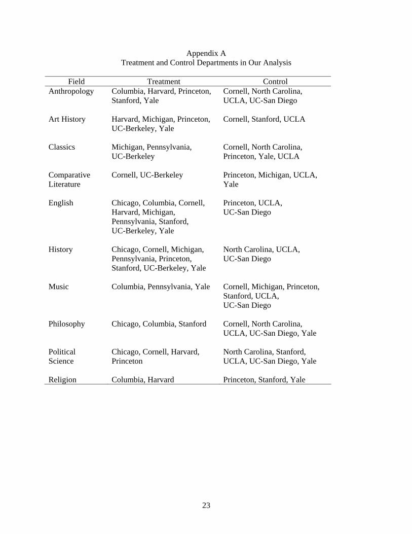
1 Appendix A lists the 44 treatment and the 41 control departments whose data are included in our analyses in this paper. The departments omitted from our analyses were ones for which no comparable department was present in the other (treatment or control) group, for which there were inaccuracies in data reporting, or that participated in the GEI but started their participation later, or terminated it earlier, than other departments.

3

programs in the treatment and control departments during the 1982-1997 period that was

conducted by Mathematica Policy Research Inc. for the Mellon Foundation. After briefly

describing the survey in the next section, section III outlines our methodological approach.

Section IV presents our empirical findings and brief concluding remarks appear in section V.

While our focus is on evaluating the effects of the GEI, we believe the methodological approach

that we use can be profitably employed in a wide range of program evaluation studies.

II. The Graduate Education Survey

The Graduate Education Survey (GES) was a retrospective survey conducted by

Mathematica Policy Research Inc. of all PhD students who had entered treatment and control

departments’ PhD programs during the 1982-1997 period.2 Between November 2002 and

October 2003, 18,671 individuals were surveyed and the GES achieved a rather remarkable

response rate of 74 percent, with 13,552 individuals responding. As might be expected, the

response rate was higher for individuals who completed their PhDs than individuals who did not

complete their PhDs and the response rates were lowest for the earliest entering cohorts of

students.

The GES was designed to obtain respondents’ views about the nature of their graduate

programs and graduate departments, their experiences while in graduate school and their post

degree (or post drop out) labor market experiences. The first section of the GES asked students

questions about their entry to their graduate programs (including type of financial aid offer), their

departments’ academic expectations and requirements and the means by which these were

conveyed to them. The second section asked questions about their interactions with their

dissertation advisors and their department, the overall learning environment in the department,

2 A more complete description of the GES and the issues discussed in this section is found in Kalb and Dwoyer (2004).

4

the time it took them to complete different phases of their programs and their publications, if

any, while in graduate school. The third section asked questions about their types of financial

support while in graduate school, and the relevance of this support to their doctoral study. The

fourth section solicited degree completion information and the following section solicited

demographic information, including marital status and the number of children in the

respondent’s family during his or her graduate study. A final section, whose data we will not use

in this paper, solicited information on their employment status at three points in time – six

months after degree completion or departure from their program, three years after that event, and

as of the survey date. A copy of the survey instrument and a detailed description of the

procedures followed during the survey are found in Kalb and Dwoyer (2004).

III. Methodological Framework

Coupled with the data previously reported to the Andrew W. Mellon Foundation by the

departments, the GES data provide an opportunity to analyze how the GEI impacted upon

characteristics of humanities and related social science doctoral program and how these

characteristics in turn influenced students’ probabilities of attrition from, and completion of, their

graduate programs. That is, it permits us to ascertain the routes via which the GEI influenced

PhD students’ attrition and completion probabilities.

While individuals were asked numerous questions in the GES about the characteristics of

their PhD programs, it is impossible for us to enter each characteristic as a separate explanatory

variable in an analysis of the students’ transition probabilities for two reasons. First, if we tried to

do this, we would quickly exhaust degrees of freedom and would be confronted with severe

collinearity problems. Second, even though the response rate to the GES was 74 percent,

response rates on individual questions were often much lower. Many survey respondents failed

5

to respond to a number of questions about the characteristics of their programs, at least in part

because some questions were not relevant for respondents who had dropped out of the programs

prior to the dissertation stage.

The strategy that we pursue to get around these problems in this paper is to compute the

average value of each program characteristic, for individuals who responded to that question, for

each entering cohort year/field/institution (for example students entering PhD study in English at

Cornell University in 1988) and to use these averages in factor analyses that combine all of these

characteristics into a smaller number of aggregated program characteristics.3 We then estimate

how the GEI influenced each of these aggregated characteristics and in turn how the

characteristics influenced students’ attrition and completion probabilities. From these two sets of

relationships, we can then estimate the routes via which the GEI influenced the PhD students’

attrition and completion probabilities.

IV. Empirical Analyses

Table 1 reports the seven factors that we have chosen to summarize the characteristics of

humanities and associated social science doctoral programs: financial, seminar, exam

requirements, departmental culture, advising, clarity, and summer. Under each factor is the set of

specific variables that we use to construct the factor that are based on responses to questions

from the GES.

For example, the financial factor is based upon respondents’ answers to questions about

the number of years of support offered to students at their time of program entry, the type of

financial support that they had during their dissertation year, whether they had fears of losing

funding during the writing of their dissertation and whether their progress toward the PhD was 3 Appendix B provides an intuitive explanation of factor analysis and a discussion of the difference between it and an alternative methodology, principle components analysis. Readers interested in more details can consult Lawley and Maxwell (1971) or Joreskog and Sorbom (1979).

6

slowed by their being employed outside the department. The seminar factor is based upon

requirements students faced to attend courses or seminars during the academic year, which were

designed to move students more quickly through the program. The exam requirements factor was

based upon efforts to modify examinations to facilitate students’ transitions through the program.

The department culture factor was based on variables reflecting the interest faculty took

in students’ work, faculty involvement in the intellectual life of the department, and whether

there was a sense of competitiveness or cooperation in the department. The advising factor was

based upon variables that reflected more desirable and higher quality advising, while the clarity

factor was based upon variables that related to departmental clarity with respect to requirements

and efforts to monitor student performance. Finally, the summer factor was based on summer

expectations set by the department to facilitate student progress through the program. In each

case, individual questions from the GES have been recoded so that higher values of a variable

indicate larger values for the factor.

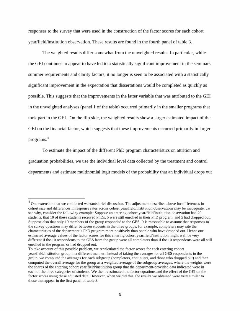
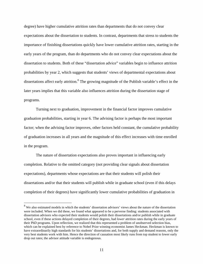
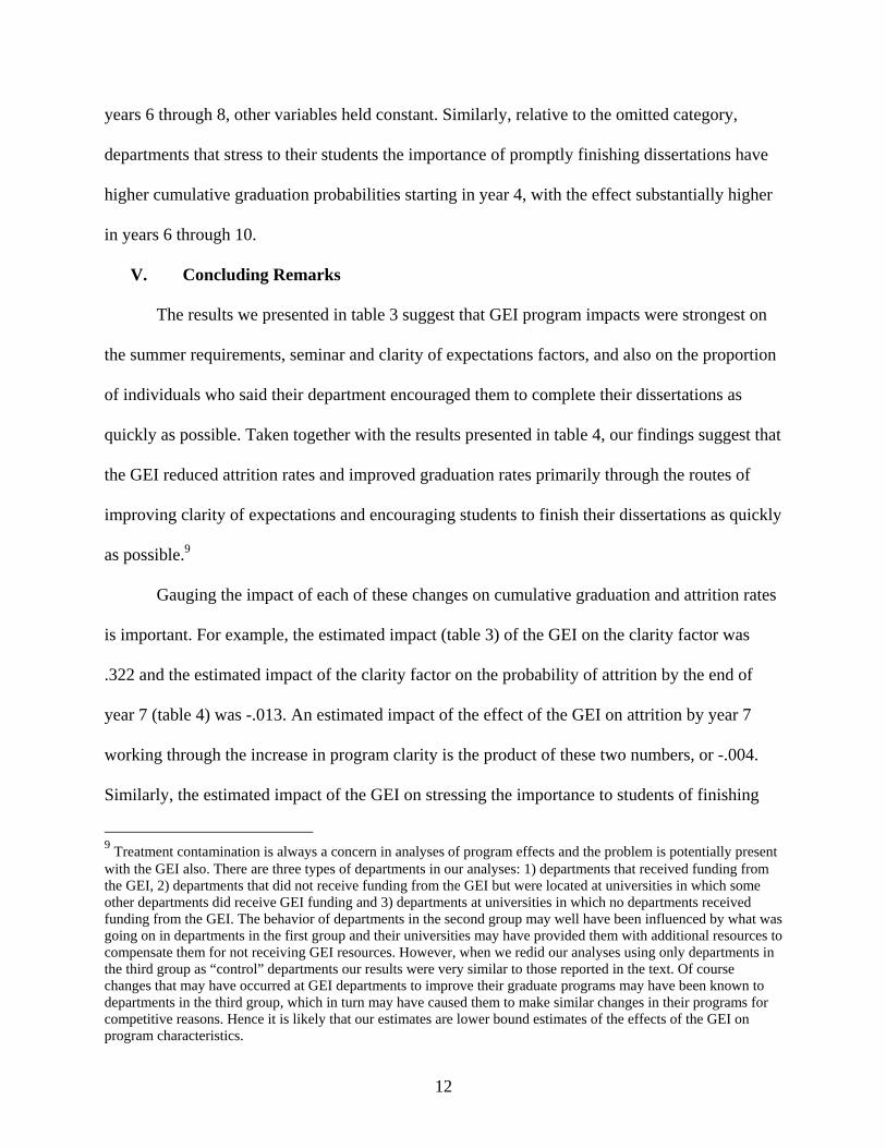
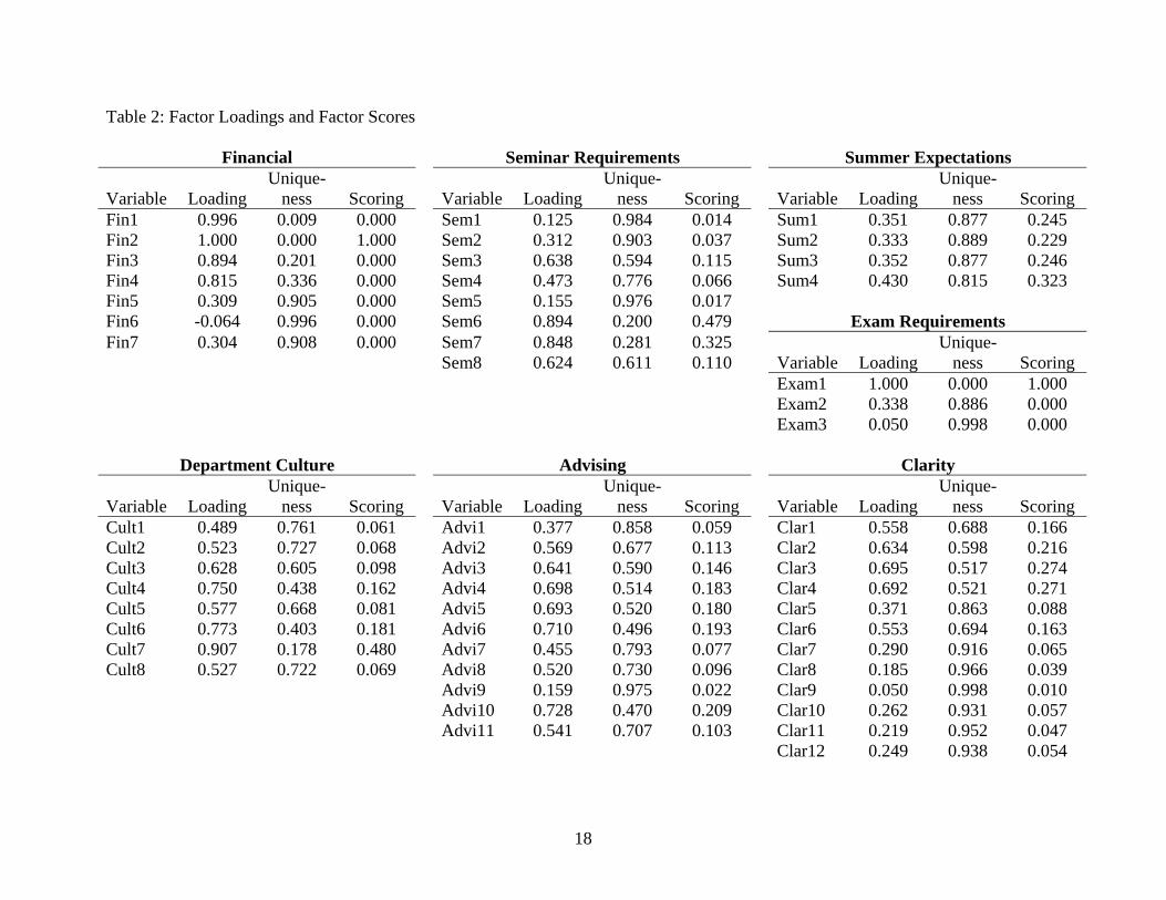
Table 2 presents our estimated factor equations for each factor. These were estimated

using the mean values of variables for each entering cohort year/field/institution for both

treatment and control departments. The factor loading coefficients can be thought of as the

regression coefficient that would emerge if we regressed the unknown factor on each of the

explanatory variables one at a time. So, for example, in the equation for the first factor, large

factor loadings are seen for the different numbers of years of financial support initially offered,

with less weight being placed on the remaining three variables. However, as the second column

indicates, many of these coefficients have large error variances (the uniqueness variable). The

factor scores found in the last column are the weights actually used to construct the factors; they

can be thought of as the regression coefficients that would emerge if we regress the unknown

7

factor on all of the variables (each in standard normal form) simultaneously. So, for example, the

most important variable in the financial factor proves to be whether the students were offered at

least two years of support when first admitted to the program, and the most important variable in

the exam factor is whether the exams students faced were tailored at least partially to their

individual research interests. Similarly, the most important variable in the seminar factor is

whether the students were required to attend a dissertation-writing seminar.

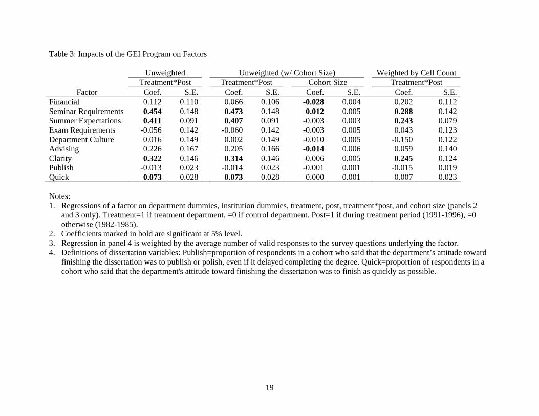
Table 3 presents our estimates of the impact of the GEI on each of the factors, as well as

on two other variables we constructed from the survey data that summarize students’ beliefs

about their departments’ expectations about dissertations. The first variable (Publish) denotes the

fraction of respondents in the entering cohort year/field/institution that said that the department

stressed the importance to them of polishing their dissertations prior to submission, even if this

delayed completion of their degree, or of publishing while in graduate school, even if this

delayed completion of their degree. The second variable (Quick) denotes the fraction of

respondents in the entering cohort year/field/institution that said that the department stressed to

them the importance of finishing dissertations as quickly as possible. These two variables do not

add up to one (indeed typically their sum is less than one half) because students were given the

option of responding that their department did not indicate its attitude towards finishing the

dissertation or that the attitudes of different members of the department were inconsistent on this

issue.

The underlying model used in the first panel of table 3 groups the data by entry cohort

year/field/institution and regresses each factor score on dichotomous variables for department

and institution, a dichotomous variable for whether the department is treatment or control

department, a dichotomous variable indicating whether the entering cohort is a pre-program

8

cohort or a cohort entering after the program was instituted, and the interaction of the latter two

variables. The coefficients of the last variable provide our estimates of the impact of the GEI on

each factor; essentially it is the difference-in-difference estimate. In order to measure longer-run

changes, students that began their PhD study between 1986 and 1990 are excluded from the

analysis, because while they entered graduate school before the GEI began in 1991, they were

eligible for financial support from the GEI starting in 1991.

The estimates presented in panel 1, in which each observation is given equal weight,

suggest that the GEI’s primary effect on doctoral programs in these fields was felt through the

seminar, summer and clarity factors and through increased encouragement to finish dissertations

as quickly as possible; these were the only four variables for which the estimated effects were

statistically significant. The second panel in the table provides similar estimates when cohort size

is added as an additional explanatory variable to the underlying models. The addition of cohort

size does not significantly change the results. Panel 3 presents the estimates of the cohort size

variable in these models – decreasing cohort size is associated with higher values for the

financial factor, lower values for the seminar factor, and higher values for the departmental

culture and advising factors. We know from our prior research that one of the actions that

departments took in response to the GEI was to reduce cohort size (Groen et al. 2004).

Entering cohort sizes, as well as the fraction of surveyed individuals that responded to the

GES, differed substantially across entering cohort years/fields/institutions in the sample. Hence

the numbers of individual observations from which the factor scores are calculated vary widely

across entering cohort years/fields/institutions and thus the variance of the factor scores varies

across observations. To control for this, we reestimated the regressions in table 3 (without the

cohort size variable included) weighting each observation by the average number of valid

9

responses to the survey that were used in the construction of the factor scores for each cohort

year/field/institution observation. These results are found in the fourth panel of table 3.

The weighted results differ somewhat from the unweighted results. In particular, while

the GEI continues to appear to have led to a statistically significant improvement in the seminars,

summer requirements and clarity factors, it no longer is seen to be associated with a statistically

significant improvement in the expectation that dissertations would be completed as quickly as

possible. This suggests that the improvements in the latter variable that was attributed to the GEI

in the unweighted analyses (panel 1 of the table) occurred primarily in the smaller programs that

took part in the GEI. On the flip side, the weighted results show a larger estimated impact of the

GEI on the financial factor, which suggests that these improvements occurred primarily in larger

programs.4

To estimate the impact of the different PhD program characteristics on attrition and

graduation probabilities, we use the individual level data collected by the treatment and control

departments and estimate multinomial logit models of the probability that an individual drops out

4 One extension that we conducted warrants brief discussion. The adjustment described above for differences in cohort size and differences in response rates across cohort year/field/institution observations may be inadequate. To see why, consider the following example: Suppose an entering cohort year/field/institution observation had 20 students, that 10 of these students received PhDs, 5 were still enrolled in their PhD program, and 5 had dropped out. Suppose also that only 10 members of the group responded to the GES. It is reasonable to assume that responses to the survey questions may differ between students in the three groups; for example, completers may rate the characteristics of the department’s PhD program more positively than people who have dropped out. Hence our estimated average values of the factor scores for this entering cohort year/field/institution might well be very different if the 10 respondents to the GES from the group were all completers than if the 10 respondents were all still enrolled in the program or had dropped out. To take account of this possible problem, we recalculated the factor scores for each entering cohort year/field/institution group in a different manner. Instead of taking the averages for all GES respondents in the group, we computed the averages for each subgroup (completers, continuers, and those who dropped out) and then computed the overall average for the group as a weighted average of the subgroup averages, where the weights were the shares of the entering cohort year/field/institution group that the department-provided data indicated were in each of the three categories of students. We then reestimated the factor equations and the effect of the GEI on the factor scores using these adjusted data. However, when we did this, the results we obtained were very similar to those that appear in the first panel of table 3.

10

of a PhD program or graduates by the end of each year of enrollment in the program.5 The

explanatory variables included in these models are an individual’s gender, race/ethnicity,

citizenship, dichotomous variables for the field in which the student was studying, and

dichotomous variables for the institution in which the student is studying. In addition, for each

individual observation, we add in the estimated values of the seven program characteristics

factors and two departmental dissertation expectation variables for the entering

cohort/field/institution.

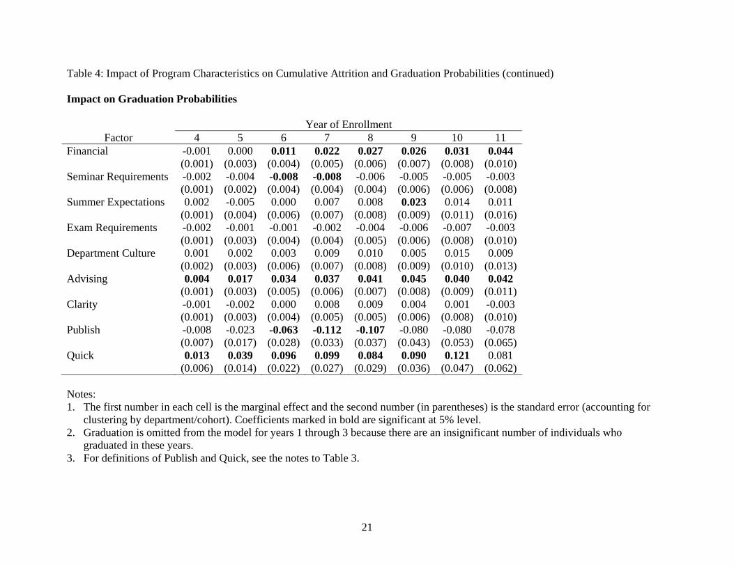
The marginal effects for the program characteristics appear in table 4.6 We estimate

impacts on the cumulative probability of attrition for years 1 to 11 and on the cumulative

probability of graduation for years 4 to 11. The marginal effects reported in the table are

estimates of the impact of a one unit change in each variable on the probabilities of attrition or

graduation by each year.

Turning first to attrition, improvements in the financial factor reduce the cumulative

probability of attrition in almost all years. The effect on the cumulative probability is largest in

the first three years, which implies that the largest effect is on early attrition.7 Having a program

with better advising and having a program whose requirements are clearer also reduces attrition

probabilities in many years. Finally, departmental expectations about the dissertation influence

attrition rates.

Departments that emphasize the importance to students of polishing their dissertations

and/or getting things published while in graduate school (even if this delayed completion of the

5 Because of the small number of students that complete their programs in years 1 to 3, we only estimate binary logit attrition equations for those years. 6 When we reestimated the models including cohort size as an additional explanatory variable, we obtained very similar results. 7 The primary variable that was important in the financial factor was offering entering students at least two years of support (see table 2).

11

degree) have higher cumulative attrition rates than departments that do not convey clear

expectations about the dissertation to students. In contrast, departments that stress to students the

importance of finishing dissertations quickly have lower cumulative attrition rates, starting in the

early years of the program, than do departments who do not convey clear expectations about the

dissertation to students. Both of these “dissertation advice” variables begin to influence attrition

probabilities by year 2, which suggests that students’ views of departmental expectations about

dissertations affect early attrition.8 The growing magnitude of the Publish variable’s effect in the

later years implies that this variable also influences attrition during the dissertation stage of

programs.

Turning next to graduation, improvement in the financial factor improves cumulative

graduation probabilities, starting in year 6. The advising factor is perhaps the most important

factor; when the advising factor improves, other factors held constant, the cumulative probability

of graduation increases in all years and the magnitude of this effect increases with time enrolled

in the program.

The nature of dissertation expectations also proves important in influencing early

completion. Relative to the omitted category (not providing clear signals about dissertation

expectations), departments whose expectations are that their students will polish their

dissertations and/or that their students will publish while in graduate school (even if this delays

completion of their degrees) have significantly lower cumulative probabilities of graduation in

8 We also estimated models in which the students’ dissertation advisors’ views about the nature of the dissertation were included. When we did these, we found what appeared to be a perverse finding: students associated with dissertation advisors who expected their students would polish their dissertations and/or publish while in graduate school, even if these actions delayed completion of their degrees, had lower attrition rates during the early years of their PhD programs. Upon reflection, we realized that this represented a problem of unobserved selection bias, which can be explained best by reference to Nobel Prize winning economist James Heckman. Heckman is known to have extraordinarily high standards for his students’ dissertations and, for both supply and demand reasons, only the very best students work with him. Hence the direction of causation most likely runs from top student to lower early drop out rates; the advisor attitude variable is endogenous.

12

years 6 through 8, other variables held constant. Similarly, relative to the omitted category,

departments that stress to their students the importance of promptly finishing dissertations have

higher cumulative graduation probabilities starting in year 4, with the effect substantially higher

in years 6 through 10.

V. Concluding Remarks

The results we presented in table 3 suggest that GEI program impacts were strongest on

the summer requirements, seminar and clarity of expectations factors, and also on the proportion

of individuals who said their department encouraged them to complete their dissertations as

quickly as possible. Taken together with the results presented in table 4, our findings suggest that

the GEI reduced attrition rates and improved graduation rates primarily through the routes of

improving clarity of expectations and encouraging students to finish their dissertations as quickly

as possible.9

Gauging the impact of each of these changes on cumulative graduation and attrition rates

is important. For example, the estimated impact (table 3) of the GEI on the clarity factor was

.322 and the estimated impact of the clarity factor on the probability of attrition by the end of

year 7 (table 4) was -.013. An estimated impact of the effect of the GEI on attrition by year 7

working through the increase in program clarity is the product of these two numbers, or -.004.

Similarly, the estimated impact of the GEI on stressing the importance to students of finishing

9 Treatment contamination is always a concern in analyses of program effects and the problem is potentially present with the GEI also. There are three types of departments in our analyses: 1) departments that received funding from the GEI, 2) departments that did not receive funding from the GEI but were located at universities in which some other departments did receive GEI funding and 3) departments at universities in which no departments received funding from the GEI. The behavior of departments in the second group may well have been influenced by what was going on in departments in the first group and their universities may have provided them with additional resources to compensate them for not receiving GEI resources. However, when we redid our analyses using only departments in the third group as “control” departments our results were very similar to those reported in the text. Of course changes that may have occurred at GEI departments to improve their graduate programs may have been known to departments in the third group, which in turn may have caused them to make similar changes in their programs for competitive reasons. Hence it is likely that our estimates are lower bound estimates of the effects of the GEI on program characteristics.

13

their dissertations promptly was .073 (table 3) and the estimated impact of this variable on

graduating by year 8 was .084 (table 4). Thus the estimated impact of the GEI on the probability

of graduating by year 8 working through the increased encouragement to students to finish their

dissertations promptly is the product of these two numbers, or .006.

While each of these effects may seem quite small, their magnitudes should be interpreted

in terms of our earlier analyses of the overall impact of the GEI on attrition and completion

probabilities. There we found that that the GEI reduced attrition rates and increased completion

probabilities at treatment departments relative to control departments by about .02 to .04 (Groen

et al. 2004). Hence the impact of the GEI on these PhD program characteristics “explains” a

substantial share of the overall effect of the GEI.10

While the GEI appears to have had an impact on characteristics of graduate programs,

there remains substantial room for improvement. Table 5 ignores the distinction between

treatment and control departments and presents summary statistics for each of the factors and

dissertation advice variables for cohorts in our sample that entered after the start of the GEI

(1991-1996). The mean value of the clarity factor was .238 across entering cohorts/departments

during this period, the 25th percentile value was -.365 and the 75th percentile was .945. The

difference between the 25th and 75th percentiles is 1.310, which is more than four times our

estimated impact of the GEI on the clarity factor. So if one could improve the clarity factor for

departments down at the 25th percentile up the level of the clarity factor for departments at the

75th percentile, one could reduce attrition by year 7 in the former departments by about .02.

Similarly, the mean value of the Quick variable was .248 in this period, but the 25th to

75th percentile range in this variable was .083 to .357, a difference of .274. This is over three

10 Groen et al. (2004) also showed that the routes via which the GEI improved attrition and graduation probabilities included reductions in entering cohort sizes and improvements in entering students’ GRE scores.

14

times the size of the estimated impact of the GEI on this variable. If one could move departments

down at the 25th percentile in terms of the Quick variable up to the 75th percentile, one could

increase the probability of students graduating by year 8 from the former departments also by

about .03.

So an important message of this analysis is that the value of the GEI is considerably

greater than the impacts on attrition and graduation probabilities that we believe it caused. The

knowledge it has provided the academic community on which factors are associated with

attrition and graduation probabilities in humanities and related social science graduate programs

should provide a map for departments and graduate deans on how to improve their programs in

the future.

Finally, we should again stress that our estimates of the effects of the GEI on the various factors,

and hence on attrition and graduation rates, may well be only lower bound estimates of the true

effects of the program. To the extent that the “control” departments in our sample were aware of

the changes that the “treatment” departments were making in their programs and emulated the

behavior of the latter, our methodology will understate the GEI’s actual effects.

15

References

Andrew W. Mellon Foundation. 1991. “Foundation Announces Major New Program in

Graduate Education.” Press Release, March 25.

Bowen, William G. and Neil L. Rudenstine. 1992. In Pursuit of the PhD (Princeton, NJ:

Princeton University Press).

Joreskog, Karl G. and Dag Sorbom. 1979. Advances in Factor Analysis and Structural

Equation Models (Cambridge, MA: Abt Books).

Jeffrey Groen, Scott Condie, George Jakubson and Ronald Ehrenberg. 2004.

“Preliminary Estimates of the Andrew W. Mellon Foundation’s Graduate Education Initiative on

Attrition Rates and Times to Degree in Humanities and Related Social Science Graduate

Programs.” Paper presented at the November 2004 NBER Higher Education Meeting,

Cambridge, MA.

Hoffer, Thomas B. et al. 2004. Doctorate Recipients from United States Universities:

Summary Report 2003 (Chicago: National Opinion Research Center).

Kalb, Laura and Emily Dwoyer. 2004. Evaluation of the Graduate Education Initiative:

Final Report (Princeton, NJ: Mathematica Policy Research Inc.).

Lawley, D.N. and A.E. Maxwell. 1971. Factor Analysis as a Statistical Method, 2nd ed.

(London: Butterworths).

16

Table 1: Variables that Enter the Factors Financial: Higher values imply more financial support Fin1 1=offered at least one year of support, 0=otherwise Fin2 1=offered at least two years of support, 0=otherwise Fin3 1=offered at least three years of support, 0=otherwise Fin4 1=offered at least four years of support, 0=otherwise Fin5 1=fellowship or stipend was primary support during dissertation stage, 0=otherwise Fin6 1=did not fear losing funding during dissertation phase, 0=otherwise Fin7 progress toward PhD was slowed by being employed outside the department (1 to 5, 5=not at all to 1=a great deal) Seminar Requirements: Higher values imply more course and seminar requirements Sem1 1=department expected the student to attend a course on research methods, 0=otherwise Sem2 1=department expected the student to attend to a course to prepare the dissertation proposal, 0=otherwise Sem3 1=department expected the student to attend a course on the dissertation process after completing the proposal, 0=otherwise Sem4 1=department expected the student to complete dissertation proposal as part of comprehensive exams, 0=otherwise [Note: Exam2=Sem4] Sem5 1=department expected the student to present their dissertation work-in-progress to other students, 0=otherwise Sem6 1=students were required to attend special workshops on dissertation writing and related topics, 0=otherwise Sem7 1=students were required to present their work at the seminars described in Sem6, 0=otherwise Sem8 1= financial support was conditional on attending the workshops described in Sem6, 0=otherwise Summer Expectations: Higher values imply greater number of summer expectations set by the department Sum1 1=expected to attend a summer course for comprehensive exams, 0=otherwise Sum2 1=expected to attend a summer workshop on dissertation proposal, 0=otherwise Sum3 1=expected to do field work, travel, or archival research prior to dissertation stage during summer, 0=otherwise Sum4 1=expected to prepare for language exams during summer, 0=otherwise Exam Requirements: Higher values imply greater effort to modify exam stage to facilitate transition from coursework to research stage Exam1 1=students were expected to have their exams tailored, at least in part, to their specific dissertation research interests, 0=otherwise Exam2 1=students were expected to complete dissertation proposal or prospectus as part of comprehensive exams, 0=otherwise [Note: Exam2=Sem4] Exam3 number of language exams required by department

17

Table 1: Variables that Enter the Factors (continued) Department Culture: Higher values imply better department culture Cult1 1=someone took special interest in their work, 0=otherwise [Note: Cult1=Advi3] Cult2 1=a faculty member took interest in their work, 0=otherwise [Note: Advi4=Cult2] Cult3 1=met socially with faculty at department functions, 0=otherwise Cult4 there was a sense of solidarity among students within the department (1 to 5, 5=strongly agree to 1=strongly disagree) Cult5 The department did not foster competitiveness among students (1 to 5, 5=strongly agree to 1=strongly disagree) Cult6 Faculty facilitated student involvement in the intellectual life of the department (1 to 5, 5=strongly agree to 1=strongly disagree) Cult7 There was a sense of personal involvement and support among faculty, students, and the department (1 to 5, 5=strongly agree to 1=strongly disagree) Cult8 progress was slowed by political struggles or frictions within the department (1 to 5, 5=not at all to 1=a great deal) Advising: Higher values imply more desirable and higher quality advising Advi1 program prepared them to teach at the collegiate level (1 to 5, 5=strongly agree to 1=strongly disagree) Advi2 program prepared them to conduct research (1 to 5, 5=strongly agree to 1=strongly disagree) Advi3 1=someone took special interest in their work, 0=otherwise [Note: Cult1=Advi3] Advi4 1=a faculty member took interest in their work, 0=otherwise [Note: Advi4=Cult2] Advi5 advising was useful in developing their dissertation prospectus/proposal (1 to 4, 1=not advised to 4=very useful) Advi6 advising was useful in researching and writing their dissertation (1 to 4, 1=not advised to 4=very useful) Advi7 advising was useful in obtaining dissertation grants (1 to 4, 1=not advised to 4=very useful) Advi8 advising was useful in obtaining an academic job (1 to 4, 1=not advised to 4=very useful) Advi9 advising was useful in obtaining a non-academic job (1 to 4, 1=not advised to 4=very useful) Advi10 progress was slowed by poor academic advising (1 to 5, 5=not at all to 1=a great deal) [Note: Advi10=Clar8] Advi11 progress was slowed by dissertation supervisor’s lack of availability (1 to 5, 5=not at all to 1=a great deal) Clarity: Higher values imply greater departmental clarity with regard to rules and better progress monitoring efforts Clar1 1=informed in writing about course requirements, 0=otherwise Clar2 1=informed in writing about policies regarding incompleteness, 0=otherwise Clar3 1=informed in writing about definition of satisfactory progress, 0=otherwise Clar4 1=informed in writing about deadlines for completing coursework and exams, 0=otherwise Clar5 1=informed in writing about department or university goals to increase PhD completion rates, 0=otherwise Clar6 1=informed in writing about departmental expectations concerning length of time to complete PhD, 0=otherwise Clar7 1=notified that there is a maximum time to complete the degree, 0=otherwise Clar8 progress was slowed by poor academic advising (1 to 5, 5=not at all to 1=a great deal) [Note: Advi10=Clar8] Clar9 1=letter grades were used to evaluate progress, 0=otherwise Clar10 1=written assignments were used to evaluate progress, 0=otherwise Clar11 1=a formal review was used to evaluate progress, 0=otherwise Clar12 1=a formal faculty committee was used to review to evaluate progress, 0=otherwise

18

Table 2: Factor Loadings and Factor Scores

Financial Seminar Requirements Summer Expectations

Variable Loading Unique-

ness Scoring Variable Loading Unique-

ness Scoring Variable Loading Unique-

ness Scoring Fin1 0.996 0.009 0.000 Sem1 0.125 0.984 0.014 Sum1 0.351 0.877 0.245 Fin2 1.000 0.000 1.000 Sem2 0.312 0.903 0.037 Sum2 0.333 0.889 0.229 Fin3 0.894 0.201 0.000 Sem3 0.638 0.594 0.115 Sum3 0.352 0.877 0.246 Fin4 0.815 0.336 0.000 Sem4 0.473 0.776 0.066 Sum4 0.430 0.815 0.323 Fin5 0.309 0.905 0.000 Sem5 0.155 0.976 0.017 Fin6 -0.064 0.996 0.000 Sem6 0.894 0.200 0.479 Exam Requirements Fin7 0.304 0.908 0.000 Sem7 0.848 0.281 0.325 Unique- Sem8 0.624 0.611 0.110 Variable Loading ness Scoring Exam1 1.000 0.000 1.000 Exam2 0.338 0.886 0.000 Exam3 0.050 0.998 0.000

Department Culture Advising Clarity

Variable Loading Unique-

ness Scoring Variable Loading Unique-

ness Scoring Variable Loading Unique-

ness Scoring Cult1 0.489 0.761 0.061 Advi1 0.377 0.858 0.059 Clar1 0.558 0.688 0.166 Cult2 0.523 0.727 0.068 Advi2 0.569 0.677 0.113 Clar2 0.634 0.598 0.216 Cult3 0.628 0.605 0.098 Advi3 0.641 0.590 0.146 Clar3 0.695 0.517 0.274 Cult4 0.750 0.438 0.162 Advi4 0.698 0.514 0.183 Clar4 0.692 0.521 0.271 Cult5 0.577 0.668 0.081 Advi5 0.693 0.520 0.180 Clar5 0.371 0.863 0.088 Cult6 0.773 0.403 0.181 Advi6 0.710 0.496 0.193 Clar6 0.553 0.694 0.163 Cult7 0.907 0.178 0.480 Advi7 0.455 0.793 0.077 Clar7 0.290 0.916 0.065 Cult8 0.527 0.722 0.069 Advi8 0.520 0.730 0.096 Clar8 0.185 0.966 0.039 Advi9 0.159 0.975 0.022 Clar9 0.050 0.998 0.010 Advi10 0.728 0.470 0.209 Clar10 0.262 0.931 0.057 Advi11 0.541 0.707 0.103 Clar11 0.219 0.952 0.047 Clar12 0.249 0.938 0.054

19

Table 3: Impacts of the GEI Program on Factors Unweighted Unweighted (w/ Cohort Size) Weighted by Cell Count Treatment*Post Treatment*Post Cohort Size Treatment*Post

Factor Coef. S.E. Coef. S.E. Coef. S.E. Coef. S.E.Financial 0.112 0.110 0.066 0.106 -0.028 0.004 0.202 0.112Seminar Requirements 0.454 0.148 0.473 0.148 0.012 0.005 0.288 0.142Summer Expectations 0.411 0.091 0.407 0.091 -0.003 0.003 0.243 0.079Exam Requirements -0.056 0.142 -0.060 0.142 -0.003 0.005 0.043 0.123Department Culture 0.016 0.149 0.002 0.149 -0.010 0.005 -0.150 0.122Advising 0.226 0.167 0.205 0.166 -0.014 0.006 0.059 0.140Clarity 0.322 0.146 0.314 0.146 -0.006 0.005 0.245 0.124Publish -0.013 0.023 -0.014 0.023 -0.001 0.001 -0.015 0.019Quick 0.073 0.028 0.073 0.028 0.000 0.001 0.007 0.023 Notes: 1. Regressions of a factor on department dummies, institution dummies, treatment, post, treatment*post, and cohort size (panels 2

and 3 only). Treatment=1 if treatment department, =0 if control department. Post=1 if during treatment period (1991-1996), =0 otherwise (1982-1985).

2. Coefficients marked in bold are significant at 5% level. 3. Regression in panel 4 is weighted by the average number of valid responses to the survey questions underlying the factor. 4. Definitions of dissertation variables: Publish=proportion of respondents in a cohort who said that the department’s attitude toward

finishing the dissertation was to publish or polish, even if it delayed completing the degree. Quick=proportion of respondents in a cohort who said that the department's attitude toward finishing the dissertation was to finish as quickly as possible.

20

Table 4: Impact of Program Characteristics on Cumulative Attrition and Graduation Probabilities Impact on Attrition Probabilities

Year of Enrollment Factor 1 2 3 4 5 6 7 8 9 10 11

Financial -0.029 -0.026 -0.022 -0.007 -0.012 -0.021 -0.023 -0.019 -0.014 -0.013 -0.011 (0.004) (0.005) (0.005) (0.010) (0.007) (0.007) (0.006) (0.006) (0.007) (0.007) (0.007)Seminar Requirements 0.002 0.005 0.005 0.014 0.009 0.008 0.006 0.006 0.005 0.005 0.001 (0.003) (0.004) (0.004) (0.008) (0.006) (0.005) (0.005) (0.005) (0.005) (0.006) (0.007)Summer Expectations 0.004 0.009 0.016 0.000 0.018 0.008 0.006 0.008 0.010 0.012 0.005 (0.006) (0.007) (0.008) (0.011) (0.010) (0.009) (0.009) (0.009) (0.009) (0.010) (0.010)Exam Requirements 0.001 -0.003 0.000 0.011 -0.001 -0.001 -0.001 -0.003 -0.006 -0.005 -0.002 (0.004) (0.005) (0.005) (0.008) (0.007) (0.006) (0.006) (0.006) (0.006) (0.006) (0.006)Department Culture -0.005 -0.001 -0.003 -0.009 -0.006 -0.005 -0.006 -0.010 -0.008 -0.003 -0.004 (0.005) (0.006) (0.007) (0.011) (0.009) (0.008) (0.008) (0.008) (0.008) (0.008) (0.009)Advising -0.012 -0.021 -0.033 -0.050 -0.058 -0.055 -0.051 -0.046 -0.047 -0.048 -0.049 (0.005) (0.005) (0.006) (0.011) (0.009) (0.008) (0.007) (0.007) (0.008) (0.008) (0.008)Clarity -0.009 -0.009 -0.012 -0.003 -0.001 -0.008 -0.013 -0.013 -0.008 -0.010 -0.006 (0.004) (0.005) (0.005) (0.008) (0.007) (0.006) (0.006) (0.006) (0.006) (0.006) (0.006)Publish -0.006 0.065 0.069 0.095 0.086 0.108 0.120 0.106 0.090 0.106 0.109 (0.028) (0.031) (0.034) (0.052) (0.043) (0.040) (0.037) (0.037) (0.038) (0.039) (0.040)Quick -0.045 -0.057 -0.051 -0.127 -0.113 -0.106 -0.074 -0.053 -0.063 -0.044 -0.074 (0.024) (0.027) (0.029) (0.046) (0.040) (0.034) (0.033) (0.034) (0.034) (0.036) (0.037) Notes: 1. The first number in each cell is the marginal effect and the second number (in parentheses) is the standard error (accounting for

clustering by department/cohort). Coefficients marked in bold are significant at 5% level. 2. Graduation is omitted from the model for years 1 through 3 because there are an insignificant number of individuals who

graduated in these years. 3. For definitions of Publish and Quick, see the notes to Table 3.

21

Table 4: Impact of Program Characteristics on Cumulative Attrition and Graduation Probabilities (continued) Impact on Graduation Probabilities

Year of Enrollment Factor 4 5 6 7 8 9 10 11

Financial -0.001 0.000 0.011 0.022 0.027 0.026 0.031 0.044 (0.001) (0.003) (0.004) (0.005) (0.006) (0.007) (0.008) (0.010)Seminar Requirements -0.002 -0.004 -0.008 -0.008 -0.006 -0.005 -0.005 -0.003 (0.001) (0.002) (0.004) (0.004) (0.004) (0.006) (0.006) (0.008)Summer Expectations 0.002 -0.005 0.000 0.007 0.008 0.023 0.014 0.011 (0.001) (0.004) (0.006) (0.007) (0.008) (0.009) (0.011) (0.016)Exam Requirements -0.002 -0.001 -0.001 -0.002 -0.004 -0.006 -0.007 -0.003 (0.001) (0.003) (0.004) (0.004) (0.005) (0.006) (0.008) (0.010)Department Culture 0.001 0.002 0.003 0.009 0.010 0.005 0.015 0.009 (0.002) (0.003) (0.006) (0.007) (0.008) (0.009) (0.010) (0.013)Advising 0.004 0.017 0.034 0.037 0.041 0.045 0.040 0.042 (0.001) (0.003) (0.005) (0.006) (0.007) (0.008) (0.009) (0.011)Clarity -0.001 -0.002 0.000 0.008 0.009 0.004 0.001 -0.003 (0.001) (0.003) (0.004) (0.005) (0.005) (0.006) (0.008) (0.010)Publish -0.008 -0.023 -0.063 -0.112 -0.107 -0.080 -0.080 -0.078 (0.007) (0.017) (0.028) (0.033) (0.037) (0.043) (0.053) (0.065)Quick 0.013 0.039 0.096 0.099 0.084 0.090 0.121 0.081 (0.006) (0.014) (0.022) (0.027) (0.029) (0.036) (0.047) (0.062) Notes: 1. The first number in each cell is the marginal effect and the second number (in parentheses) is the standard error (accounting for

clustering by department/cohort). Coefficients marked in bold are significant at 5% level. 2. Graduation is omitted from the model for years 1 through 3 because there are an insignificant number of individuals who

graduated in these years. 3. For definitions of Publish and Quick, see the notes to Table 3.

22

Table 5: Summary Statistics for Factors, 1991-96 Entering Cohorts Percentile

Factor Mean Std. Dev. 25th 75thFinancial 0.459 0.843 -0.090 1.239Seminar Requirements 0.150 1.277 -0.574 0.371Summer Expectations 0.213 0.838 -0.316 0.624Exams 0.308 1.123 -0.358 1.570Department Culture 0.167 1.082 -0.503 0.913Advising 0.177 1.041 -0.476 0.872Clarity 0.238 1.105 -0.365 0.945Publish 0.130 0.156 0.000 0.200Quick 0.248 0.223 0.083 0.357

23

Appendix A Treatment and Control Departments in Our Analysis

Field Treatment Control

Anthropology Columbia, Harvard, Princeton, Stanford, Yale

Cornell, North Carolina, UCLA, UC-San Diego

Art History Harvard, Michigan, Princeton,

UC-Berkeley, Yale Cornell, Stanford, UCLA

Classics Michigan, Pennsylvania,

UC-Berkeley Cornell, North Carolina, Princeton, Yale, UCLA

Comparative Literature

Cornell, UC-Berkeley Princeton, Michigan, UCLA, Yale

English Chicago, Columbia, Cornell,

Harvard, Michigan, Pennsylvania, Stanford, UC-Berkeley, Yale

Princeton, UCLA, UC-San Diego

History Chicago, Cornell, Michigan,

Pennsylvania, Princeton, Stanford, UC-Berkeley, Yale

North Carolina, UCLA, UC-San Diego

Music Columbia, Pennsylvania, Yale Cornell, Michigan, Princeton,

Stanford, UCLA, UC-San Diego

Philosophy Chicago, Columbia, Stanford Cornell, North Carolina,

UCLA, UC-San Diego, Yale Political Science

Chicago, Cornell, Harvard, Princeton

North Carolina, Stanford, UCLA, UC-San Diego, Yale

Religion Columbia, Harvard Princeton, Stanford, Yale

24

Appendix B A Reader’s Guide to Factor Analysis

The substantive problem we face in this paper is trying to determine the routes via which

the Andrew W. Mellon Foundation’s Graduate Education Initiative had effects on the attrition rates and graduation rates of PhD students in the humanities and associated social sciences. The Foundation’s Graduate Education Survey provides us with information on a large number of variables that relate to the nature of the students’ graduate programs, including ones related to financial support, seminar requirements, exam requirements, departmental culture, departmental advising, clarity of requirements and expectations and summer support (table 1).

These variables are, not surprisingly, both numerous and highly intercorrelated, so that

one cannot simply include 50 or so of them as explanatory variables in the outcome equations. Therefore a method is needed to find lower dimensional combinations of the variables that summarize the information they provide. The way we do this is described below. For ease of explanation, assume that there is just one aspect of the program we which to capture, for example, financial generosity. We have a number of measures of this which are highly intercorrelated. Adding all of them to the outcome equation would result in a collinearity problem, which in turn would lead to estimates that are both imprecise and unstable. We could just choose a subset of the variables to include in the analysis. To do this would discard all of the information in the unused variables and would lead to problems of omitted variable bias. Moreover, it is not obvious how to choose the subset to keep. We instead use information from all of the observed variables. Essentially, we find a (linear) combination of the observed variables that represents our best estimate of the common component financial generosity. Let’s start with an explicit example. Suppose that there are four observed characteristics that reflect this common component. Let yit be the measured variable for individual i and variable t. The index i reflects the number of observations and goes from 1 to N, while the index t reflects the variables and goes from 1 to 4 in this example. Let ci be the underlying common “factor” which we’ll think of as financial generosity, and suppose that the data were generated by the following model:

yi1 = β1ci + εi1 (A.1) yi2 = β2ci + εi2

yi3 = β3ci + εi3 yi4 = β4ci + εi4

We assume that the εit’s have mean zero and are uncorrelated with one another and with

ci, though they may have different variances. (Those orthogonality conditions essentially define, in a statistical sense, what ci is.) If the common factor ci were observable this would simply be a system of regression equations. Since it is not observable we want to find a (linear) combination of the observed yit’s that best predicts ci. That is, we want

25

(A.2) E*(ci | yi) = γ’yi where yi is the vector (yi1 , yi2 , ... yiT)’. One can show that the optimal set of weights is (A.3) [ ] )c,y(Cov)y(V ii

1i

−=γ

Thus, γ is a function of the underlying parameters of the model. If we knew those then we would know γ. Because we don’t know them, we must use estimates of the parameters to form an estimate of γ. However, because ci is not observable we cannot estimate the system of regression equations implied by (A.1). Instead, the information about the parameters comes from the variance matrix of the observed variables. Let Var(ci) = ϕ2 Var(εit) = σt

2 Cov(εit , εis) = 0 for t ≠s

)(V

000000000000

i

24

23

22

21

ε=

⎥⎥⎥⎥⎥

⎦

⎤

⎢⎢⎢⎢⎢

⎣

⎡

σσ

σσ

=Σ

),,,( 4321 ′ββββ=β

Because ci is not observed we need to set scale by normalizing one parameter. The

tradition in psychology is to normalize ϕ2 = 1. An equivalent, and easier to explain, normalization is to set β1 =1 , that is, we measure the β’s for the other variables relative to that of the first variable. Given the latter normalization, the variance matrix for the observed yi is

( ) =Σ+ϕβ′β=Ω 2

⎥⎥⎥⎥⎥

⎦

⎤

⎢⎢⎢⎢⎢

⎣

⎡

σ+ϕβϕββσ+ϕβϕββϕββσ+ϕβϕβϕβϕβσ+ϕ

24

224

243

23

223

242

232

22

222

24

23

22

21

2

where we’ve just filled in the upper triangle of the matrix since it is symmetric. We can now solve for the parameters as functions of the elements of the variance matrix:

13232 /ωω=β

2122 /βω=ϕ

2133 /ϕω=β

2144 /ϕω=β

26

211

21 ϕ−ω=σ

22222

22 ϕβ−ω=σ

22333

23 ϕβ−ω=σ

22444

24 ϕβ−ω=σ

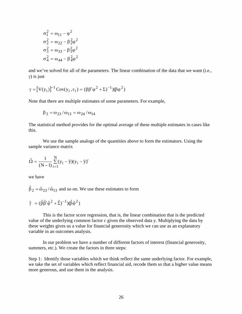
and we’ve solved for all of the parameters. The linear combination of the data that we want (i.e., γ) is just

[ ] ))()()c,y(Cov)y(V 212ii

1i βϕΣ+ϕβ′β==γ −−

Note that there are multiple estimates of some parameters. For example,

142413232 // ωω=ωω=β The statistical method provides for the optimal average of these multiple estimates in cases like this.

We use the sample analogs of the quantities above to form the estimators. Using the sample variance matrix

∑ ′−−−

=Ω=

N

1iii )yy)(yy(

)1N(1ˆ

we have

13232 ˆ/ˆˆ ωω=β and so on. We use these estimates to form

)ˆˆ)()ˆˆˆˆ(ˆ 212 ϕβΣ+ϕβ′β=γ −

This is the factor score regression, that is, the linear combination that is the predicted value of the underlying common factor c given the observed data y. Multiplying the data by these weights gives us a value for financial generosity which we can use as an explanatory variable in an outcomes analysis.

In our problem we have a number of different factors of interest (financial generosity, summers, etc.). We create the factors in three steps: Step 1: Identify those variables which we think reflect the same underlying factor. For example, we take the set of variables which reflect financial aid, recode them so that a higher value means more generous, and use them in the analysis.

27

Step 2: Compute the average value of each variable, for individuals who respond to the underlying question, for each group defined by entering cohort year/field/institution. Step 3: Do the factor analysis to find the factor score regression defined above.

We then repeat those steps for each of the factors.

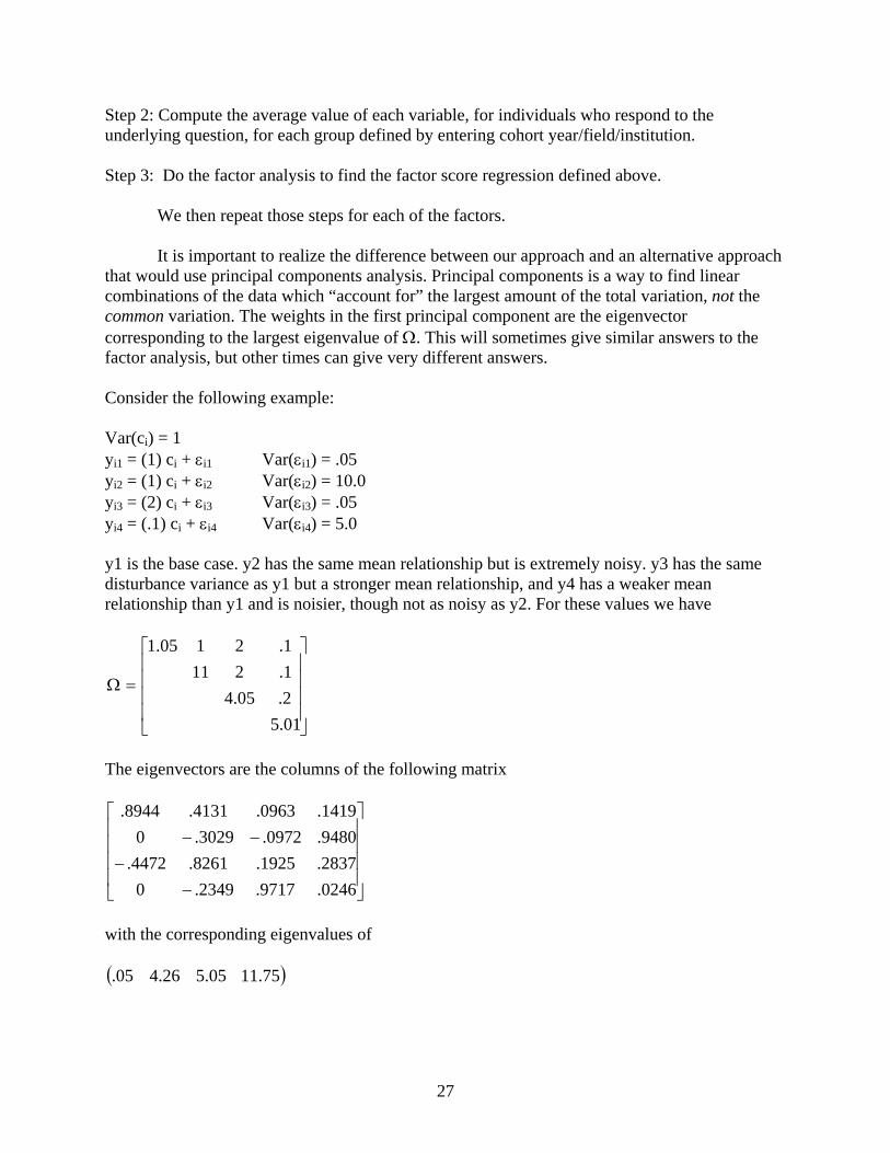
It is important to realize the difference between our approach and an alternative approach that would use principal components analysis. Principal components is a way to find linear combinations of the data which “account for” the largest amount of the total variation, not the common variation. The weights in the first principal component are the eigenvector corresponding to the largest eigenvalue of Ω. This will sometimes give similar answers to the factor analysis, but other times can give very different answers. Consider the following example: Var(ci) = 1 yi1 = (1) ci + εi1 Var(εi1) = .05 yi2 = (1) ci + εi2 Var(εi2) = 10.0 yi3 = (2) ci + εi3 Var(εi3) = .05 yi4 = (.1) ci + εi4 Var(εi4) = 5.0 y1 is the base case. y2 has the same mean relationship but is extremely noisy. y3 has the same disturbance variance as y1 but a stronger mean relationship, and y4 has a weaker mean relationship than y1 and is noisier, though not as noisy as y2. For these values we have

⎥⎥⎥⎥

⎦

⎤

⎢⎢⎢⎢

⎣

⎡

=Ω

01.52.05.41.2111.2105.1

The eigenvectors are the columns of the following matrix

⎥⎥⎥⎥

⎦

⎤

⎢⎢⎢⎢

⎣

⎡

−−

−−

0246.9717.2349.02837.1925.8261.4472.9480.0972.3029.01419.0963.4131.8944.

with the corresponding eigenvalues of ( )75.1105.526.405.

28

so that the last column of the matrix contains the weights for the first principle component. Note that the weight on y2 is very large, more than six times larger than the weight on y1.

In contrast, the pattern of weights from the factor analysis is very different. We have, using the formula above γ = (.1978, .0010, .3950, .0002) and then normalizing them so that they have unit length, like the principal component, yields weights of γ* = (.4472 , .0022 , .8944 , .0004)’

We see that the factor analysis puts higher weight on variables with small error variances and strong relationships to the common factor, that is, it “rewards” the variables that reflect the common components of variation rather than idiosyncratic components.