1

Insecticide Resistance Monitoring, Mechanisms and Management Manual

K. R. Kranthi B. Sc (Ag), M. Sc (Ag), Ph. D

Central Institute for Cotton Research (Indian Council of Agricultural Research)

Post Bag o. 2, Shankarnagar PO, Nagpur 440 010 Phone: 07103-275549, 36. Fax: 07103-275529; e-mail: cicrngp@rediffmail.com

2

Photographs: Achyut Bharose, S. N. Syed & K. R. Kranthi An output of the Common Funds for Commodities project 'Sustainable control of the cotton bollworm, Helicoverpa armigera in small scale production systems'. Copyright: Central Institute for Cotton Research, Nagpur. First Edition: 2005; Citation: K. R. Kranthi. 2005. 'Insecticide Resistance -Monitoring, Mechanisms and Management Manual'. Published by CICR, Nagpur, India and ICAC, Washington Published by the Director, Central Institute for Cotton Research, PB.No 2, Shankarnagar PO. Nagpur

3

Contents

3-5 Foreword 6 Preface 7 Introductory note 8 Chapter 1. Introduction 9 Chapter 2. Conventional Bioassays 11 2.1 Field dose assay 11 2.2 Discriminating dose assay / Diagnostic dose assay 12 2.3 Log dose probit assay 16 Chapter 3. Protocols for resistance monitoring 17 3.1 Sampling and rearing techniques 17 3.2 Laboratory cultures of H. armigera 19 3.3 Precautions in H. armigera rearing 21 3.4 Diet preparation for H. armigera and S. litura 22 3.4.1 Larval diet 22 3.4.2 Moth diet 22 3.4.3 Diet for long term rearing of H. armigera 23 3.4.4 Larval diet 23 3.5 Diet preparation for E. vittella and P. gossypiella 24 3.5.1 Larval diet 24 Chapter 4. Bioassays 25 4.1 Commonly used bioassay methods 29 4.1.1 Topical application 30 4.1.1.1 Preparation of insecticide solutions for topical and 30 glass vial residue bioassays 4.1.1.2 Topical treatment 32 4.1.2 Glass vial residue test 33 4.1.2.1 Preparation of insecticide solutions for diet, 34 residual and immersion bioassays 4.1.3 Surface coating/residual bioassays 35 4.1.4 IRAC Methods 36 4.1.4.1 IRAC Method No. 1 36 4.1.4.2 IRAC Method No. 7 37 4.1.4.3 IRAC Method No. 8 38 4.1.5 Immersion methods 39 4.1.6 Sticky card assay 40 4.1.7 Diet incorporation methods for oral toxicants 41 4.1.7.1 Preparation of Cry1Ac toxin solutions for bioassays 41 4.1.7.2 Preparation of Cry toxins from recombinant clones 42 4.1.7.3 Diet incorporation 43 4.1.7.4 Diet incorporation for filter paper bioassays 44 4.1.7.5 Surface coating of semi-synthetic diet 44

4

Chapter 5. Bioassays with transgenic plants 45 5.1 Bioefficacy of Bt-transgenic plants 46 5.2 Whole plant efficacy assessment 47 5.3 Cry1Ac estimation using bioassays 47 5.4 Log dose probit assay 49 Chapter 6. Statistical analysis of bioassay data 50 6.1 Statistical analysis of dose-mortality responses 50 6.2 Statistical analysis of diagnostic dose data 53 Chapter 7. Synergism studies 54 7.1 Evaluating synergistic ratios 55 Chapter 8. Metabolic resistance mechanisms 57 8.1 Enzyme classification 58 8.2 Biochemical routes of insecticide detoxification 59 8.3 Mono-oxygenases 61 8.3.1 Cytochrome P450, cytochrome p420 and Cytochrome b5 67 8.3.1.1 Substrate-induced spectral kinetics of cytochrome P450s 70 8.3.2 NADPH cytochrome c reductase assay 72 8.3.3 Ethoxy coumarin O-Dealkylation (ECOD) assay 73 8.3.4 Resorufin O-Dealkylation assays 75 8.3.5 MROD (Methoxyresorufin demethylase) 75 8.3.6 EROD (Ethoxyresorufin deethylase) 76 8.3.7 p-Nitroanisole O-Demethylase assay 77 8.3.8 Benzphetamine N-Demethylase assay 79 8.3.9 Peroxidation of Tetramethylbenzidine (TMBZ) assay 80 8.3.10 Aldrin epoxidation 81 8.3.11 Purification of cytochrome P450 reductase 83 8.4 Hydrolases 84 8.4.1 Phosphotriester hydrolases 87 8.4.2 Carboxylesterase assay 88 8.4.2.1 Preparation of �-naphthol standard curve 89 8.4.2.2 Staining of non-specific Esterases on native PAGE 90 8.4.2.3 Purification of isozymes 91 8.4.2.4 Alternate protocol (Purification of isozymes) 91 8.4.3 Epoxide hydrolases 92 8.5 Glutathione-S-transferase

93 8.5.1 Glutathione-S-transferase assay 93 8.5.1.1 Purification of Glutathione transferases 94 8.5.1.2 Staining for GST activity on native PAGE 95 Chapter 9. Target site insensitivity 96 9.1 Neurophysiological assay for pyrethroid resistance 98 9.2 Acetyl cholinesterase 100 9.2.1 Acetyl cholinesterase assay 101 9.2.2 Staining for AChE activity on native PAGE 101

5

Chapter 10. Genetics of resistance 102 10.1 Determining the mode of inheritance 103 10.2 Estimating the number of alleles conferring resistance 106 10.3 Identifying sex-linked resistant alleles 107 10.4 Estimating the initial frequency of resistant alleles. 109 10.5 Resistance Risk assessment 111 10.6 Estimate changes in resistant allele frequencies in field populations 112 Chapter 11. Resistance diagnostic kits 116 Chapter 12. Resistance management strategies 120 12.1 Cotton pests and natural control 120

12.1.1 Sucking pests 121 12.1.2 The bollworms 122 12.1.2.1 Helicoverpa armigera 122 12.1.2.2 Pectinophora gossypiella 123 12.1.2.3 Earias vitella and Earias insulana 123 12.1.3 Leaf feeding caterpillars 124

12.2 Conventional pest management systems 125 12.3 Rationale for development of the IRM technology 126 12.4 IRM strategies 131 12.5 Basic operations to ensure minimum pest problems in cotton 134 12.6 IRM strategies for Bt-cotton 135

12.6.1 Sucking pest control in Bt-cotton 136 12.6.2 Other useful strategies to mitigate resistance in Bt-cotton 136

Chapter 13. Dissemination methods 137

13.1 Village selection 137 13.2 Style of presentation 137 13.3 Syllabus 137 13.4 Technology for a price 137 13.5 Staff 139 13.6 Farmer participation 138 13.7 Awareness campaign. 138

References 139 About the Author 153

6

Foreword ‘Insecticide Resistance - Monitoring, Mechanisms and Management Manual’ is a techniques book that contains methods and protocols related to the assessment, diagnosis and management of insecticide resistance in insect pests. Though the book deals mostly with insecticide resistance in the cotton bollworm, Helicoverpa armigera, the methods described are almost universally applicable to most insect species. The manual is an outcome of several years of work on resistance at the CICR, Nagpur. The first part deals with the basic principles of insect culture maintenance and bioassays. The theory of diagnostic and discriminating dose assays has been dealt with, in detail. The chapters on biochemical methods describe the principles and protocols used in biochemical assays most commonly used to elucidate metabolic mechanisms of resistance. Nerve insensitivity and genetics of resistance have been dealt with, in a clear and lucid style to make beginners feel comfortable while starting studies on the topics. Resistance management strategies and the extension methods recommended in the manual are based on extensive field experience. Though the strategies are described for cotton pest management under Indian conditions, specifically for 2004, the principles behind the strategies would be useful to all the stakeholders interested in formulating resistance management strategies applicable for their regions or countries. The Central Institute for Cotton Research has been spearheading the cause of sustainable cotton pest management through efficient management insect resistance to insecticides. The resistance management group has been addressing the problem of resistance on all aspects related to the subject. The group has worked on resistance monitoring and mechanisms for more than 12 years and has formulated strategies based on the data generated. The strategies, now commonly referred to as IRM (Insecticide Resistance Management) are being implemented successfully by state agricultural universities, state agricultural departments, NGOs and ICAR institutes in more than 100,000 hectares of 450 villages of 9 cotton growing states for over three years, under the leadership of CICR, Nagpur. The immense support from the Ministry of Agriculture under the TMC-MM-II project; the Common Funds for Commodities ‘Sustainable control of the cotton bollworm, Helicoverpa armigera in small-scale production systems’project, and the ICAR, is gratefully acknowledged. I would like to commend and congratulate Dr K. R. Kranthi, for having written and compiled all the relevant methods and protocols necessary for resistance studies. I am confident that the manual will be extremely useful for students, researchers, planners and extension workers. New Delhi, 6th Dec 2004

C. D. Mayee Chairman, ASRB,

ICAR, Krishi Anusandhan Bhavan, New Delhi Former Commissioner of Agriculture,

Ministry of Agriculture, Government of India,.

7

Preface Handbooks are useful companions in laboratories. There have been a few manuals/handbooks earlier containing useful protocols to detect and monitor insecticide resistance. Dr Nigel Armes, NRI, UK and Dr Alan McCaffery, Syngenta, UK, compiled some very informative techniques for resistance monitoring in their training manual draft copies produced from ICRISAT in1993 and Reading University in 1995 respectively. This handbook is inspired by their efforts. It has been designed to serve as a ready reference on the methods used in insecticide resistance monitoring and management. The techniques presented here, are what we have been using for years. They are fairly robust, simple and can be used quite easily. There are many standard basic biochemistry and molecular biology protocols that could have been added to the current compilation, but that would make the list superfluous and repetitive. Though, the main emphasis in the manual has been on protocols related to bioassays on lepidopteran insects, specifically H. armigera, the basic protocols presented here can be adapted to several other insect species. I have also included bioassay protocols for insects with reference to transgenic Bt-cotton varieties. The biochemical, genetic and molecular methods to elucidate insecticide resistance mechanisms are expected to be highly useful for researchers and students. Resistance management strategies are ever changing. With scientific advances being made continuously; there will be many more methods that will be added over time. Molecular methods are advancing at a tremendous pace. Recent techniques such as microarrays, real-time PCR and other PCR related methods used in resistance research have not been included in this edition. The applications of these techniques in unraveling the mechanisms of insect resistance to insecticides are just beginning to appear in research journals. The resistance management strategies presented here are designed for Indian farming conditions and represent the state of art in resistance management science until 2004. There can certainly be local adjustments to suit regional pest population dynamics. The strategies, of course will change with the advances in pest management research in future. Dr C. D. Mayee, Chairman, ASRB, ICAR, and ex-Director, CICR, has been a great pillar of strength and support for all our endeavors in research and development. I am highly indebted to him for the enormous encouragement and support. Dr SheoRaj, Head, Crop Protection Division and Dr S. K.Banerjee, Principal Scientist, Entomology, have always spearheaded the cause of IRM for sustainable pest management in cotton and have been highly supportive throughout. Prof. Derek Russell, NRI, UK, a great friend and co-researcher, has been keen for a long time that a handbook such as this is published for the benefit of students and fellow researchers. I thank him for his support and for having gone through the draft critically. Mr Anant Chaudhary, Achyut Bharose and Syed N Shahzad deserve a special mention for their assistance. Dr Rafiq Chaudhry, ICAC helped this project and supported it all through. Finally I would like to express my sincere thanks to Dr Sandhya Kranthi, my wife for being my main source of strength. I fervently hope that this handbook will be useful for researchers, extension functionaries, and all the stakeholders of cotton pest management. Nagpur. 2005

K. R. Kranthi

8

Introductory Note This volume fills a need long-felt by workers in the area of insecticide resistance measurement, mechanisms and management. We have had standardized techniques for the monitoring of resistance in the Insecticide Resistance Action Committee (IRAC) ‘methods’. These have been enormously useful in allowing comparisons across laboratories and geographic areas and are described here. However, the need to understand the underlying biochemical mechanisms of resistance and the patterns of their genetic inheritance and how to implement that information in improved pesticide management in the field has led to the development of a range of new methods for which there has been no standard text which students and practitioners can turn to. This volume fills that need. It arises out of the large body of work on insecticide resistance in Asia’s main agricultural pest, the cotton bollworm Helicoverpa armigera, and particularly in India and builds on the seminal training course run by Dr Alan McCaffery and colleagues at Reading University, UK in 1996 at which so many of the key resistance researchers in the region attended. However, many, even most, of the techniques have been developed since that time and are certainly applicable beyond the bollworm species for which it was originally developed. Any compilation of methods has to draw on the work of many people and every effort has been made to acknowledge the sources of the information presented. However, it must be said that Dr Keshav Kranthi of the Central Institute for Cotton Research in India has played an enormously important leadership role in all aspects of the understanding of resistance issues in cotton pests in the region and is himself the developer and refiner of many of the techniques presented here. Work using these techniques underpins the highly successful National Insecticide Resistance Management programme in cotton (2002-2007), which is supported by the Government of India and is technically backstopped by the Central Institute for Cotton Research and currently involves more than 100,000 farmers across all the main cotton producing states. It is therefore wholly appropriate that Dr Kranthi should be the author and compiler of this volume, which will be a key foundation for the development of our understanding of resistance issues in years to come. Support for the underlying research which has given rise to this volume has been provided through a series of networked projects first in India in the 1990s under Indian government and UK Department for International Development funding and later across India, China, Pakistan and UK with the support of the Common Fund for Commodities/ International Cotton Advisory Committee project (2001-2005) in which the national governments (Indian Council for Agricultural Research, Pakistan Central Cotton Committee, the National Agricultural Technology Extension Service Centre in China, DFID in the UK and IRAC International) were active partners. This current work draws particularly on the contributions of the collaborators in that programme. This volume will have done its job if it catalyses further discoveries and more advanced methodologies in resistance research.

Derek Russell 24th November 2004 Natural Resources Institute

of the University of Greenwich, UK Project manager CFC/ICAC-014

‘Sustainable control of cotton bollworm, Helicoverpa armigera in small-scale cotton production systems’

9

Chapter 1 Introduction Insecticide resistance is a result of accelerated microevolution. Under selection pressure the fittest survive, multiply and spread. It results from the survival and spread of resistant insect genotypes that have the capability to endure insecticide selection pressures in the environment. Insect development of resistance to insecticides is an inevitable consequence of insecticide use for pest control. When the frequency of resistant phenotypes increases to a certain level in field populations, control efficacy with the concerned insecticide becomes economically unacceptable. But poor efficacy under field conditions is not always due to insecticide resistance. Amongst other factors, the quality of technical grade material used, the formulation, the application dose and the method of application can also play an important role in impairing field control. However, if resistance is the major factor, field control failure is inevitable, irrespective of quality, quantity or methods of application. Thus resistance eventually is the single most important phenomenon that threatens sustainable pest management. It is therefore important to detect resistance when it is at incipient levels and monitor its increase and geographical spread so that appropriate measures can be initiated to curtail its increase. The major objectives of resistance detection and monitoring must be to eventually ensure effective and sustainable pest management. Applications of resistance detection and monitoring are as follows:

1. Resistance monitoring methods help to document geographical and temporal variability in population responses to insecticide selection pressures. Monitoring helps to keep track of the precise changes in resistant phenotype frequencies occurring in field populations.

2. Resistance detection bioassays determine the relative efficacy

of insecticides for a given field population. In immediate practical terms, resistance detection helps in avoiding ineffective molecules and assists in making a proper recommendation of alternative molecules that are less resisted and can effectively control insect pests. This prevents wastage of pesticide applications that would have otherwise harmed the environment without actually having served the designated purpose of pest management. Thus, resistance detection serves an early warning of the impending problem of uncertain levels of pest control under field conditions.

3. The bioassays diagnose and confirm the causes of pest control

failure by specific insecticides under field conditions. 4. Resistance monitoring helps to evaluate the impact of

resistance management strategies, which have been implemented.

10

Resistance detection methods are based on the following assays: 1. Conventional bioassays: Diagnostic dose assays and log-dose probit (LDP) assays are the two most commonly used methods of detecting, monitoring and documenting resistance. 2. Biochemical assays: Resistant strains may be characterized by the presence of a unique or over-expressed defence mechanism, that is either absent or if present may be expressed at lower levels in the susceptible strains compared to that in the resistant strains. Such strains can be characterized by biochemical assays that can detect and monitor insecticide resistance. 3. Molecular assays: Molecular assays are specifically designed based on observed mutations in the resistant allele itself or based on DNA fragments closely linked to the resistant allele.

4. Immunological assays: Immunoassays are generally based on antibodies raised against a major biochemical molecule that confers insecticide resistance in insects. The assays either use ELISA or the dip-stick format to detect the frequency of resistant insects in field populations.

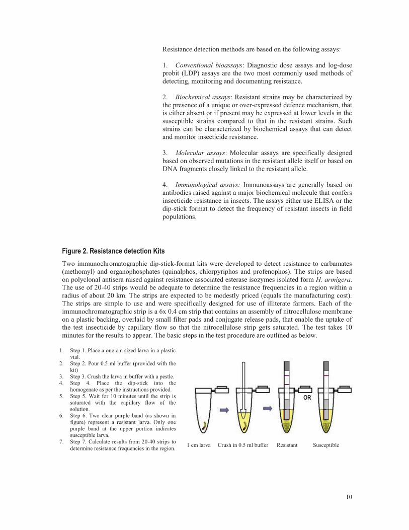
Figure 2. Resistance detection Kits Two immunochromatographic dip-stick-format kits were developed to detect resistance to carbamates (methomyl) and organophosphates (quinalphos, chlorpyriphos and profenophos). The strips are based on polyclonal antisera raised against resistance associated esterase isozymes isolated form H. armigera. The use of 20-40 strips would be adequate to determine the resistance frequencies in a region within a radius of about 20 km. The strips are expected to be modestly priced (equals the manufacturing cost). The strips are simple to use and were specifically designed for use of illiterate farmers. Each of the immunochromatographic strip is a 6x 0.4 cm strip that contains an assembly of nitrocellulose membrane on a plastic backing, overlaid by small filter pads and conjugate release pads, that enable the uptake of the test insecticide by capillary flow so that the nitrocellulose strip gets saturated. The test takes 10 minutes for the results to appear. The basic steps in the test procedure are outlined as below.

1. Step 1. Place a one cm sized larva in a plastic vial.

2. Step 2. Pour 0.5 ml buffer (provided with the kit)

3. Step 3. Crush the larva in buffer with a pestle. 4. Step 4. Place the dip-stick into the

homogenate as per the instructions provided. 5. Step 5. Wait for 10 minutes until the strip is

saturated with the capillary flow of the solution.

6. Step 6. Two clear purple band (as shown in figure) represent a resistant larva. Only one purple band at the upper portion indicates susceptible larva.

7. Step 7. Calculate results from 20-40 strips to determine resistance frequencies in the region. 1 cm larva Crush in 0.5 ml buffer Resistant Susceptible

OR

11

Chapter 2 Conventional bioassays

2.1 Field dose assay A field dose in laboratory bioassays is used to distinguish between insects that get killed and those that survive at the field application rate. The method is based on conducting bioassays with a particular life stage of the insect that represents the most damaging stage, and the populations of which get killed at proportions equivalent to the mortality in field with the recommended dose. Field application rates are generally guided by commercial and logistic considerations. If the technology is cost effective, it is possible that the chemical companies may recommend application rates that may be several fold well above the diagnostic dose. In such a case the field application rate continues to kill resistant individuals under field conditions, while the laboratory bioassays based on diagnostic dose show development of resistance to the molecule. On the other hand, if the technology is expensive, it is possible that commercial companies would want to use the product at an optimum dose that is affordable to the farmer yet provide effective management of the target pest. Such a dose may or may not be above the diagnostic dose. If it is less than the diagnostic dose, then the product may start losing field efficacy but the laboratory assays using an appropriate diagnostic dose may not show resistance as yet. Hence, a field dose assay, that is calibrated to give parallel mortality in the laboratory compared to that which a product gives under field conditions, especially on the most damaging stage of the pest, would be useful from the resistance management perspective. Initially dose-mortality curves must be determined for the designated target stage of the susceptible strain under field conditions and the proportional relationship of the recommended dose with the LC99 is calculated. A field dose assay can then be designed using the same proportional relationship with the discriminating dose. For example if the recommended dose of an insecticide is 0.01% and the LC99 under field conditions for second instar H. armigera is 0.001%, then the proportional relationship would be 0.01/0.001 = 10. Thus if the discriminating dose for the insecticide is 0.1 μg/μl per second instar H. armigera, the field dose would be 0.1 x 10 = 1.0 μg/μl per larva. The method relies on the assumption of dose-mortality in laboratory and field assays.

12

2.2 Discriminating dose assay / Diagnostic dose assay A diagnostic dose is expected to distinguish resistant from susceptible insect phenotypes. It is very important to develop a reliable diagnostic dose that can differentiate between resistant and susceptible phenotypes. If resistance diagnostic test has to be meaningful, ideally the designated diagnostic dose should kill all susceptible insects and spare all resistant insects to correlate with field efficacy of the insecticide. Thus a diagnostic dose could be a discriminating dose that differentiates between SS and RS/RR, but not between RS and RR. Discriminating doses can be calibrated to differentiate between any two of the three genotypes RR, RS and SS, if the dose-mortality regression slopes of the three genotypes do not overlap, if resistance is monogenic, autosomal, non-recessive and if resistant and susceptible strains, homozygous with respect the resistant allele are available. These doses can then be used to monitor the changes in resistant allele frequencies in field populations. Such doses are determined by conducting toxicological assessment of genetic crosses. The LD50, LD99.9 LD0.1 of the parents, F-1 progeny and progeny of reciprocal backcrosses are calculated. If resistance is not inherited as a recessive trait, the discriminating dose would be equivalent to the LD0.1 of the F-1 progeny, which could be almost equivalent to the LD50 of the backcross (SS x RS) progeny and would correspond to ≥ LD99.9 of the susceptible and ≤ LD0.1 of the resistant strains. The dose would discriminate RS genotypes from the SS and would be very useful in not only monitoring for the change in resistance frequencies but assist in calculation of changes in resistant allele frequencies, if the treated population was at Hardy-Weinberg equilibrium. Similarly as mentioned in the introductory part, it is also possible to derive a dose that can distinguish between RR and RS genotypes by obtaining LD50 of the backcross (RR x RS) progeny. This should be ≥ LD99 of F1 hybrid progeny and ≤ LD1 of the RR homozygous parent strain. In the absence of a well defined resistant and susceptible homozygous strains, the discriminating dose is deduced from LD99.9 of the baseline susceptibility data obtained from whatever laboratory susceptible strains are available and a wide range of strains collected from various geographical zones to fairly represent population variability in susceptible field strains. Note that field strain susceptibility is generally quite variable and one strain alone should not be used. Such an exercise can be carried out with field populations only before the insecticide would have inflicted any selection pressure. Generally the most common and simplest method of determining the discriminating dose has been through estimation of the LD99 of susceptible populations. This pre-supposes that resistant phenotypes do not get killed at this dose. But, we do not always know that resistant alleles exist at a frequency of < 0.01 in the susceptible populations tested. It is possible that there may not have been any resistant alleles in the susceptible strain used for the assay and that these may exist in field

13

populations, and therefore that the diagnostic dose thus derived may overestimate resistance. Hence, one way of deriving a diagnostic dose is through several bioassays on large populations of field-collected insects so as to ensure that pre-existing resistant alleles are sampled. Determining a diagnostic dose can be complicated if inheritance of resistance is recessive or incompletely recessive or polygenic. A recessively inherited resistant trait will have heterozygous genotypes, which show dose-mortality regression slopes that closely overlap with those of the homozygous susceptible genotypes. The diagnostic dose would thus depend on the magnitude of recessive inheritance. Completely recessive or incompletely recessive inheritance can lead to a diagnostic dose that may be grossly inadequate and can be several times less than the dose required to distinguish resistant homozygous genotypes. Similarly, dominant or incompletely dominant inheritance can shift the dose-mortality lines of the heterozygous genotypes closer to that of the resistant homozygous genotype and away from that of the susceptible genotype, thus the diagnostic dose derived based on susceptible strains may also be incapable of being able to distinguish truly resistant genotypes. The fact that laboratory selection processes generally select for many alleles, thus resulting in strains that are polygenic, compounds the problem. In our experience, in most cases field selected strains have been found to be resistant to a particular toxin, due to a single major allele, but laboratory selection for a few generations subsequently, appears to be selecting for genes with additive effects. It is thus important to keep in mind the genetics of inheritance of the resistant allele while determining reliable diagnostic doses that are based on proper genetic and sturdy bioassay methods, which can reflect field efficacy of the toxins. It is possible to adjust slopes of dose-mortality regression curves using various bioassay techniques and then decide on the bioassay that gives slopes of the resistant and susceptible insects in a manner that the LD99 of the susceptible phenotype just overlaps the LD1.0 of the resistant phenotype. An appropriate method of fixing a reliable diagnostic dose would be to 1. Determine the dose-mortality regression of resistant heterozygous and homozygous genotypes and the LD99 of the susceptible homozygous genotype; 2. Examine the predicted mortality of the resistant heterozygous or homozygous genotype at LD99 dose of the susceptible homozygous genotype. The dose would not qualify for resistance diagnostic purposes if it kills more than 30% of the heterozygous genotype (Ffrench-constant and Roush, 1990) or worse if it also kills more than 30% of the resistant genotype. If the LD0.1 of the heterozygous resistant genotype is greater than LD99 of the susceptible genotype, it should be preferred. Alternatively the LD0.1 of the homozygous resistant genotype can be considered if it greater than LD99 of the heterozygous genotype if the slopes of heterozygous and susceptible genotype overlapped extensively, as is the case with recessive or incompletely recessive traits. The experiments can be conducted by isolating the resistant homozygous genotypes from field strains using the F2 screen methods and conducting bioassays on progeny of genetic crosses with resistant and susceptible strains.

14

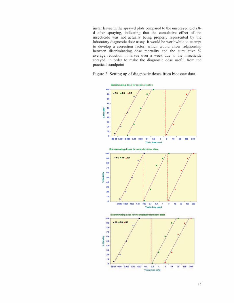
Once the baseline is established, the entire data set can be subjected to log dose probit analysis to derive LD99.9 values, which may be representative of the discriminating dose. Ideally, if the discriminating dose results correlate with field levels of insect mortality, it would be a useful indicator from the resistance management perspective. However, in many cases, it is difficult to assess how laboratory bioassays can actually correlate to field efficacy of a pesticide. But, from the resistance management perspective, the discriminating dose is an important tool to monitor changes in resistance in field populations. Once the discriminating dose is finalized, the sample size of the test population depends on the accuracy with which the dose is able to distinguish between the resistant and susceptible genotypes/phenotypes and the probable frequency of occurrence of the resistant allele in field populations. Higher frequencies of the resistant allele will require lower sample size for acceptable accuracy. At low frequencies, the sample size required for accurate estimation of resistant allele frequency may be prohibitively high. Diagnostic dose assays may or may not correlate to field efficacy of insecticides, because they are not calibrated to estimate field efficacy. The main purpose of a diagnostic dose is to distinguish between resistant and susceptible phenotypes. Field application rates of insecticides are determined by commercial considerations and can be several times more or less than the equivalent of the diagnostic dose at the point of delivery to the insect. However, if a diagnostic dose can indicate efficacy of insecticides under field conditions, it has twin advantage of being used as practical tool to recommend effective insecticides. To give a practical example, in our experience, lab measured resistance to pyrethroids at reasonably high levels of 50 - 100-fold on third instar larvae, may not greatly impact on H. armigera control in the field, because although the pesticide may not control third instar and older stage larvae it kills moths, neonates and younger larvae effectively due to contact action, which results in a good acceptable level of pest control. Therefore an overall change in cumulative effects of the insecticide on all stages of the target pest would need to be quantified and correlated in terms of the net effect on third instar larvae, before the mortality at discriminating dose would be used as an indicator of field efficacy of the chemical. Formulating such experiments to correlate laboratory measured resistance using a particular larval stage with cumulative effects of the insecticide on the target pest under field conditions can be demanding. In a simple exercise, we sprayed pyrethroid in 150 sq M plots in three replicates. The sprayed fields were surrounded by unsprayed fields. Pre-spray count one day before spraying and post spray counts for all stages of larvae were taken on alternate days up to 8 days in the sprayed and unsprayed fields. Eggs were collected from areas adjacent to the experimental plots a week before the fields were sprayed. Larvae were reared to third instar and topically treated with discriminating doses of Fenvalerate 0.2 μg/μl. Interestingly 20 % third instar mortality with Fenvalerate 0.2 ug/ul, correlated well with a 15 + 4 % mortality of third instar larvae in the field experiment (based on the pre-spray 2nd instar and post spray 4th instar counts on 2-d after spray), but there were 60 + 6 % fewer 4th

15

instar larvae in the sprayed plots compared to the unsprayed plots 8-d after spraying, indicating that the cumulative effect of the insecticide was not actually being properly represented by the laboratory diagnostic dose assay. It would be worthwhile to attempt to develop a correction factor, which would allow relationship between discriminating dose mortality and the cumulative % average reduction in larvae over a week due to the insecticide sprayed, in order to make the diagnostic dose useful from the practical standpoint Figure 3. Setting up of diagnostic doses from bioassay data.

16

It must be emphasized here that what ever method is used, if the resistance magnitude does not correlate accurately with pest control levels under field conditions, the exercise of monitoring is of little practical value to pest management. However, even if the laboratory measured resistance level correlates to the pest control level in the field, it does not necessarily represent overall field efficacy, due to factors related to economic thresholds and density dependence. For example, if the initial H. armigera infestation levels were at 5 larvae per plant, low levels of resistance 20-30% resulting in 70-80 % mortality at the recommended field rate can still leave pest numbers equivalent of the economic threshold levels of one larva per plant, which will be construed as pest control failure. On the other hand, if the initial infestation levels average one or fewer larvae per plant, it is possible that even relatively high levels of resistance at 60-70% resulting only 30-40 % mortality can result in residual pest levels below the economic thresholds and may be perceived by farmers as satisfactory pest control. Hence, for pest management to be effective, it is important to adhere to the recommendations of pesticide applications at economic threshold levels on the basis of regular examination of fields in order to deal with populations before they reach the outbreak stage. The major advantages of the discriminating dose assays are 1. The test insect numbers can be small (≈ 100). 2. The assay can detect small increases in the frequency of the

resistant insect genotypes.

3. It is simple to comprehend from a practical standpoint, provided that it indicates the probable mortality % under field conditions and hence is informative for pest management.

The major disadvantages are: 1. The assay becomes saturated at high levels of resistance and

cannot distinguish between populations differing in variable degrees of resistance beyond the saturation point that shows at 95 –100 % resistance to the discriminating dose.

2. It does not indicate the magnitude of resistance 3. It may not diagnose resistance properly, if calibrated only from

homozygous susceptible strains.

2.3 Log dose probit assay Log dose probit assays are based on toxicological assessments by subjecting insect populations to serial dilutions of insecticides to determine a dose-mortality regression response. At least 5 concentrations of the toxicant are tested on each population. The dose response can be determined as LD10, LD50, LD90, LD99 etc from the regression equation. The LD50 represents the dose that kills 50 % of the test population.

17

Chapter 3

Protocols for resistance monitoring

3.1 Sampling and rearing techniques Sampling and rearing techniques are specific for each species. The techniques described here have been followed successfully for H. armigera, and may be applicable to some related lepidopteran species.

1. H. armigera eggs are collected from host crops and weeds. H. armigera eggs can be found most readily on terminal foliage, bracts of squares, flowers and green bolls of cotton plants; leaves and pods of pigeonpea, chickpea, vegetables, weeds (Legascea mollis, Acanthospermum spp. Chenopodium album and Datura spp.) and flower heads of sunflower during the peak flowering phase of the plants.

2. Excised plant parts harbouring H. armigera eggs are

transported in cool boxes to the insectary/laboratory and transferred immediately into diet rearing trays. It is essential to transfer eggs, especially from plant parts of cotton, so as to avoid exposure of neonate larvae to Cry1Ac toxin if the host plant happens to be Bt-cotton.

3. Two eggs per well are transferred, on to the inner walls of

12-well rearing trays containing semi-synthetic diet. A soft camel hairbrush wetted with 0.1% sodium hypochlorite solution is used to gently dislodge the eggs from the plant parts and to smear them on to the walls of diet rearing trays.

4. Each diet-rearing tray is covered with a semi-permeable

thin plastic wrap, and covered with lid. The semi-permeable wrap prevents escape of neonate larvae.

5. The rearing trays are incubated at 25 + 10C and 70 + 5 %

R.H in insectary or in a BOD incubator.

6. Neonates start hatching in one or two days after the eggs are transferred into the trays.

7. Two day old first instar larvae are pale cream opaque in

appearance and are referred to as ‘white stage’. These larvae can be used for diet incorporation discriminating dose or log dose probit bioassays for assaying Cry toxins or insect growth regulating compounds.

8. Four days after hatching, the larvae reach early second

instar and must be transferred into individual cells. Late second instar and older stages are cannibalistic and start biting each other if left together. early second instar larvae can be used for insecticide leaf surface coating assays.

18

9. If the diet and rearing conditions are optimum and well

suited for larval growth, the larvae reach third instar on the sixth day after hatching. Third instar larvae can be sorted on 30 - 40 mg weight basis, transferred on to fresh diet and treated topically with the discriminating dose of the insecticide or with serially diluted technical grade solutions in acetone for dose mortality curve construction.

10. The minimum sample size for each discriminating

insecticide dose is 100 larvae and for log-dose probit assays, 250 larvae at 50 larvae per concentration.

11. If laboratory cultures are to be established from field-

collected larvae for resistance monitoring purposes, at least 100 - 300 larvae are necessary to set up a population of 1000 – 2000 larvae for the insecticide discriminating dose or log-dose probit assays.

12. Ideally moths raised from the field-collected larvae must be

single paired and the resulting progeny pooled together to represent the larval collection. This is necessary to avoid overestimating or underestimating resistance due to polyandry, polygamy in mass mated H. armigera.

13. The moth pairs can be held individually in small jars of 20

cm x 25cm (diameter x height), kept at 25 + 20 C and RH 75-80%. Jars are covered on the top with muslin cloth and contain a strip of muslin cloth for oviposition. Cotton swabs, soaked in a solution containing 5 % each of honey and sucrose are suspended along the walls of the jars and changed three times a week.

14. The larvae are transferred on to diet soon after hatching.

Rearing and bioassay procedures are same as that followed for the larvae hatching from field-collected eggs.

19

3.2 Laboratory cultures of H. armigera.

The best way to initiate setting up laboratory cultures is to begin the culture from field-collected eggs. 1. Eggs can be surface sterilized and generally do not carry

any diseases. Field collected larvae may harbour parasitoids and can also spread infections.

2. Field collected eggs are transferred from plant parts to the

wells of multi-cell insect rearing trays containing diet at the rate of 2 per well. After hatching, larvae reach late sixth instar in 13-14 days and are transferred to tubs containing sawdust for pupation.

3. If field collected larvae are used, they would be transferred

individually into single wells of multi-cell insect rearing trays containing diet.

4. Diseased or parasitized larvae must be discarded

immediately. To avoid disease spreading through the colonies, especially with NPV or stunt viruses, field collected material should be quarantined for at least one generation before integrating into the colony.

5. Late sixth instar larvae stop feeding just before pre-pupal

stage and start wandering in search of a site for pupation. At this stage, they must be transferred into tubs (20 cm dia x 8 cm h) containing sterile sawdust. Each tub can accommodate 20-25 pupae. Care must be taken to ensure that the pre-pupae are not injured or disturbed. Pre-pupae construct a pupation cell and pupate in 2-3 days.

6. The fully-formed pupae can be removed from the tub 4-5

days later and sexed. Pupae are surface sterilised with 1-2% sodium hypochlorite solution, after which they are washed with distilled water, wiped with soft tissue paper and placed on sterile sawdust in cups with ventilated lids. Pupae are kept at 24-250C and 10:14 hour light:dark photoperiod.

7. Male moths are light jade-green while females are light

brown in colour. Moths generally emerge shortly after midnight and mate 2-3 days after emergence. Oviposition starts a day after mating and continues for 6-8 days. If moths are over-fed or under-fed, longevity and fecundity are severely affected. It is preferable to starve the moths for about 12 hours after emergence. It is also important to change the diet (5% honey + 5% sucrose in water swabs) frequently to prevent fermentation, which may lead to moth mortality. Under ideal conditions each moth lays about 500-2000 eggs.

20

8. It is important to maintain a humidity of 75-80% during hatching, to prevent neonates from desiccating. Eggs are light yellow in colour when freshly laid and turn brown to black 2-3 days later, just before hatching. Infertile eggs turn brown and shrivel and can be easily differentiated from fertile eggs at 10 x magnification. Freshly laid eggs must be surface sterilised for at least 5 minutes with 1-2% sodium hypochlorite solution, after which they should be washed with distilled water and placed in a humid chamber.

9. Soon after hatching, the larvae are transferred on to semi-

synthetic diet. Brushes and forceps that are used to transfer larvae should be periodically disinfected with a 2% sodium hypochlorite solution.

10. Since larvae are cannibalistic, it is preferable to avoid

crowding at the early stages. Two-three neonates can be placed in a single cell of the rearing trays. However once larvae reach second instar, they tend to injure and consume other larvae in vicinity and hence must be kept singly in each cell of the rearing tray.

11. Initially, larvae should be transferred to fresh diet after 4-5

days, before they reach second instar, but it is necessary to change diet every alternate day or sometimes daily thereafter. It is important that the larvae should not starve at any stage before pupation.

12. Larvae are reared at 25 + 20 C at 14:10 hour light:dark

photoperiod. Larvae reared under short day lengths for one generation or under insufficient light levels for a few generations can develop into diapausing pupae.

13. There are six larval instars and larval duration generally

extends to 15-22 days. Each instar is characterised by a constant head capsule width. The head capsule widths for the 1 – 6 instars are 0.25-0.29 mm; 0.36-0.44 mm; 0.64-0.84 mm; 0.90-1.24 mm; 1.50-1.88 mm and 2.00-2.88 mm respectively (Armes et al., 1992).

21

3.3 Precautions in H. armigera rearing. Laboratory cultures of Helicoverpa armigera can be successfully established and reared continuously for at least 10-14 generations without any problem, if adequate care is taken to maintain proper rearing conditions. The following steps may help in successful maintenance of the laboratory cultures.

1. It is very important to clean and sterilise all equipment and containers using hypochlorite, autoclaving, exposure to sunlight and or germicidal lamps before re-use. Diet rearing trays, moth chambers, forceps and brushes are to be regularly decontaminated in 5% sodium hypochlorite and rectified spirit. The working bench surfaces and floor of the rearing room must be regularly cleaned and disinfected with rectified spirit and 5% hypochlorite.

2. Helicoverpa armigera cultures can be very difficult to

maintain if proper care is not taken to ensure clean sanitation and regular disinfection of cultures and culturing conditions. Some of the most problematic diseases are NPV (Nuclear Polyhedrosis Virus), microsporidian protozoa- Nosema spp, fungus - Aspergillus spp. and a range of bacteria. NPV infected larvae appear creamy white in the terminal stages and liquefy rapidly thereby spreading the virus. Nosema affected larvae stop feeding, lose weight, have a shrivelled cuticle, appear dark and stay still unless prodded. The terminal stages are similar to that of NPV infection, where the body liquefies to release the microsporidian particles. Bacteria and fungi spoil the diet and can cause persistent problems in cultures.

3. One of the best ways to get rid of larvae harbouring latent

infection of HaNPV (nuclear polyhedrosis virus) and Nosema spp. is to retain only larvae that reach the third instar stage by the 6th day after hatching. HaNPV and Nosema infected larvae have a slow growth rate and the slow growing larvae must be discarded. This helps in keeping cultures healthy. Diseased and dead larvae must be disposed immediately by removing the entire rearing tray without opening it in the culture room.

4. Eggs and pupae must be regularly surface sterilised.

5. Regular exposure to scales over long periods may lead to respiratory allergic reactions in laboratory staff. It is advisable to remove scales every day using vacuum cleaners if available. It is preferable to wear dust mask and apron to prevent inhalation of allergenic particles or their contact with the skin.

Pupae can be sexed based on distinct abdominal characteristics by viewing the ventral abdomen using 10 x magnification and maintained separately till they are mixed, three days after adult emergence.

22

3.4 Diet preparation for H. armigera and S. litura:

Recipe for H. armigera larval diet gm. Chickpea flour (Kabuli type) 160 Wheat germ (substitute sorghum leaf powder for S. litura)

60

Sorbic acid 1.7 Dried yeast 53 Ascorbic acid 5.3 Methyl paraben 3.3 Aureomycin® 2.5 Formaldehyde 10% ml 13.5 **Anti mould solution, ml (optional) 2 Agar 16 Double distilled water ml 1200

** The anti mould solution contains 5 % phosphoric acid and 45 % propionic acid in sterile water.

3.4.1 Larval diet 3.4.2 Moth diet 1. Add measured quantities of chickpea flour, wheat germ,

sorbic acid, ascorbic acid, methyl paraben and Aureomycin® into a large bowl. Add 500 ml of pre-boiled warm water, and stir thoroughly to mix well.

2. Dissolve 53 gm active dried yeast in 350 ml water and boil for 5 min.

3. Add 16 gm agar to 350 ml water, disperse well and boil for 5 min.

4. Mix the yeast and agar solutions, boil for 5 min and add to the bowl containing other diet ingredients. Mix well using a blender.

5. Add 13.5 ml 10% formaldehyde and 2 ml anti-mould solution if necessary. Mix thoroughly using a bender.

6. Transfer the hot diet into soft plastic squeeze-bottles, close with lids having spouts trimmed to 1 cm, and dispense the diet into wells of multi-cell trays.

7. Allow the trays to cool in laminar airflow under UV lamp for 2-3 hours to sterilize the diet surface.

8. Certain diet ingredients such as chickpea flour and wheatgerm may have to be autoclaved before use to prevent bacterial spoilage.

9. It may be necessary sometimes to coat the diet surface with 0.01 % of antibiotic solutions such as ampicillin, amoxycillin or streptomycin.

10. The rearing trays can be stored at 4-80C for a week.

1. Dissolve 5 gm each of

sucrose and honey to 90 ml sterile water, boil for 5 minutes and simmer for a further 15 minutes.

2. Ensure that the solution is

sterile. 3. Once the solution is cooled,

add 0.2 g each of ascorbic acid and methyl hydroxy parabenzoate. Mix well and store at 40C for 1- 2 weeks.

4. Use sterile absorbent cotton

wads to soak the solution and place them in the moth jars. Change the wads at least thrice a week.

5. The moth diet can be used

for any lepidopterans.

The procedures of larval and moth diet preparation for S. litura are the same as above.

23

3.4.3 Diet for long term rearing of H. armigera

Recipe for H. armigera larval diet gm Wheat germ 80 Chickpea flour 30 Sorbic acid 1.5 Sucrose 40 Wessons salt 10 Casein 40 Dried yeast 20 Cholesterol 1.5 Choline chloride 10 % ml 10 Ascorbic acid 4 multivitamin tab 1 Formaldehyde 10% ml 4 **Anti mould solution, ml 2 Agar 24 DD Water ml 1100

** The anti mould solution contains 5 % phosphoric acid and 45 % propionic acid in sterile water. 3.4.4 Larval diet

1. Add measured quantities of all the diet ingredients, (except agar, yeast, formaldehyde and anti mould solution) into a large bowl. Add 400 ml of pre-boiled warm water, and stir thoroughly to mix well.

2. Dissolve active dried yeast in 400 ml water and heat till it

begins to boil.

3. Add agar to the yeast solution, disperse well and boil for 5-7 min.

4. Add the hot agar-yeast solution to the bowl containing other

diet ingredients. Mix well using a blender.

5. Add formaldehyde and anti mould solution if necessary. Mix thoroughly using a bender.

6. Pour the diet in rearing trays.

7. Allow the diet to cool in laminar airflow under UV lamp for

1 h to sterilize the diet surface.

8. The diet can be stored at 4-80C for a week.

9. Wheat germ may have to be autoclaved before use to prevent bacterial spoilage.

24

3.5 Diet preparation for E. vittella and P. gossypiella:

Recipe for larval diet P. gossypiella E. vittella gm gm Cotton seed flour 120 KOH 22 % ml. 6 Acetic acid (25%) ml 16.4 Methyl paraben 2 Wheat germ 60 96 Sucrose 17 39 Wessons salt 12 12 Casein 20 44 Dried yeast 5 19 Choline chloride 10 % ml 10 12.5 multivitamin tab 1 1 Aureomycin® 1 1 Formaldehyde 10% ml 4.5 10 Agar 24 24 Sorbic acid 2 Cholesterol 1.25 Ascorbic acid 5 DD Water ml 1000 1100

* The diet recommended for E. vittella can be used for any of the three bollworms. 3.5.1 Larval diet

1. Add measured quantities of all the diet ingredients, (except agar, yeast, formaldehyde and anti mould solution) into a large bowl. Add 400 ml of pre-boiled warm water, and stir thoroughly to mix well.

2. Dissolve active dried yeast in 400 ml water and heat till it begins to boil.

3. Add agar to the yeast solution, disperse well and boil for 5-7 min.

4. Add the hot agar-yeast solution to the bowl containing other diet ingredients. Mix well using a blender.

5. Add formaldehyde and anti mould solution if necessary. Mix thoroughly using a bender.

6. Pour the diet on Whatman® filter paper sheets. 7. Allow the sheets to cool in laminar airflow under UV lamp

for 1 h to sterilize the diet surface. 8. Cut the sheets into 3 x 3 cm strips. Place the strips in small

cups 4 x 3 cm (dia x h) and release 10 larvae per cup. It is recommended to rear neonates on natural diet for a day before they are released on semi-synthetic diet.

9. Change the strips thrice a week. 10. The diet-coated sheets/strips can be stored at 4-80C for a

week. 11. Wheat germ may have to be autoclaved before use to

prevent bacterial spoilage.

25

Chapter 4

Bioassays The bioassay methods should closely simulate field conditions to ensure predictability of control efficacy in the field from data obtained through lab-measured resistance. However, based on several practical considerations resistance detection and monitoring methods are developed in such a manner so as to ensure that the bioassays are reliable, replicable, consistent and robust enough not to be influenced by variations in operator skills, materials, extraneous factors and handling procedures. For example, direct bioassays on simulated field conditions using larvae of varying resistant levels, were designed and used to monitor resistance. But, due to space and operational constraints, such assays can be performed only on a limited sample size. Over the past two decades, bioassay methods based on leaf-dip, larval dip, topical application and vial-residue were developed as viable alternatives to simulated field conditions. Following are the important factors that influence bioassays:

1. Stage of the insect: The toxic effects of an insecticide can be highly age and stage dependent. Insecticides are known to exhibit variable toxicity to different life stages of insects. For example, lepidopteran adults and early instars are known to be more susceptible to insecticides as compared to older stage larvae. Pyrethroid resistance in H. armigera is explicitly expressed in the third instars, when it is relatively easy to distinguish resistant from susceptible larvae through diagnostic assays (Daly et. al., 1988). Hence the standard topical dose assay is carried out on the third instars. The application of 1μl technical grade insecticide solution in acetone on the third instars was found to cover the pro-thoracic region optimally. On younger larvae, the insecticide tends to drip down the larva and contaminates the diet surface. Young H. armigera larvae are used in the leaf residual bioassays to monitor insecticide resistance in Pakistan and China. It must however be pointed out that the assay results can be variable because resistance may not be manifested in younger larvae, H. armigera does not feed readily on cotton leaves. Moreover, the physiological variability of the leaf can also contribute to the variance in bioassays. Moths are generally used in adult vial tests as it was found to be convenient to use pheromone trapped H. virescens moths for resistance monitoring at field sites. Topical application of insecticide can also be done by treating the ommatidia with a 1μl technical grade insecticide solution in acetone, but has rarely been used for resistance monitoring.

2. Choice of insecticide: Within a class of insecticides, some

molecules are more resisted than others. For example, several pyrethroid resistant H. armigera strains showed more resistance to deltamethrin than to cypermethrin or

26

fenvalerate. Hence resistance monitoring with any specific insecticide molecule may not be representative of the entire class of compounds. However for the sake of convenience most laboratories choose a compound that shows a median resistance response compared to other molecules of the same class.

3. Bioassay response: Most bioassays rely on mortality as the

toxic response. However, some compounds cause severe growth regulating effects in susceptible strains, which are overcome by resistant strains. In such cases, EC50, MIC50 or IC50 are calculated instead of LD50, to determine a median growth regulating response. Recently, such studies with Cry toxins are gaining prominence.

4. Method of application: Topical application through Potter’s

tower, microapplicators; or residue bioassays using glass, paper, leaf for contact poisons; or per-os application, diet-incorporation of the toxin, diet surface coating for oral toxins; are some of the main methods of applying toxins to organisms in bioassays. Because of the ease in handling, and the reasonable levels of accuracy in dispensing known amount of toxin on the test insects, topical application has emerged as the most preferred methods of toxin application for conventional insecticides. Diet incorporation and surface coating are being increasingly used for Cry toxins. It is important that the method adopted should represent proper bioactivity of the compound. For example, topical bioassay with indoxacarb does not represent its toxicity adequately because its main action is as an oral toxicant. Similarly some compounds are more water-soluble and are not very suited for topical application.

5. Bioassay environment: When insects are being subjected to

bioassays, it is necessary to maintain optimum conditions for insect growth. For H. armigera, the temperature and humidity are maintained at 25 + 10C, and 70 + 5 % relative humidity. Sub-optimal temperatures or R.H cause large variability in bioassay response.

6. Diet: Ideally, bioassays should measure only bioefficacy of

insecticide, all the rest of factors being equal. One of the factors that are likely to cause the greatest impact on the susceptibility response of organisms to toxicants is diet. Unsuitable diet can vitiate or enhance the toxic response. It is important to ensure that the larvae get fresh diet in frequent intervals over the entire period of bioassay. Semi-synthetic diets have the advantage of being consistent. They can be commonly used across geographical locations with minimal variation of dietary influence on the organism. Natural diet such as leaves or plant parts can be very different due to the age of the plant part; stage of the plant and variety. Environmental stress to plants and the poor feeding capability of H. armigera on certain plant parts can contribute to variability in bioassay results.

27

7. Health of the organism: Bioassay results obtained with

field-collected larvae frequently over-estimate toxic effects, because of health factors. Field collected larvae may harbour parasitoids, and diseases, which make them vulnerable to the toxic effects of insecticides. Unhygienic conditions in insectaries can also significantly contribute to errors in bioassays. It may not be possible to distinguish between resistant and susceptible insect genotypes in populations that are a mix of healthy and unhealthy individuals. One of the recommended strategies adopted for resistance monitoring is therefore to collect eggs of the target insect species directly from fields, rear them to the appropriate stage and then conduct bioassays.

8. Sampling: The samples collected for resistance monitoring

should represent the distribution of resistance in field populations of insects. Samples collected from a small patch of crop may have been derived from a single pair or at the most a few pair of moths, which may not be representative of the resistance profile of the normal field populations. Similarly, F1 progeny resulting from mass mating of moths obtained from only a few larvae (30-40) may also not be a representative sample, because of the chance of only a few moths (sometimes just one or two pairs) contributing disproportionately to the progeny. Moreover, polygamy in H. armigera may also significantly skew the frequency of resistant alleles in the progeny. Hence, sampling of 1000-2000 eggs from widely separated fields to represent 4-5 sq km of potential hosts, would constitute a reasonable sample size, considering the moth dispersal range of 1-2 km per night.

9. Sample size: Small sample sizes can result in misleading

bioassay interpretation. The sample size depends on the probable frequency of resistant insects in the populations being sampled. Roush and Miller (1986) define the sample size at 100 individuals, with a discriminating dose based on the LD99 of susceptible strains, when resistance levels are expected to be greater than 10 %, and presuming that only resistant insect genotypes survive the discriminating dose. But, with the same discriminating dose, at least 1500 larvae would be required to detect resistant genotypes with 95 % confidence if the frequency of resistance is 1 %. However, with an accurate discriminate dose that kills 99.9 % susceptible and 0.1 % of resistant individuals, a sample size of only 300 would be required to detect resistant alleles at 95 % probability if the resistant genotype frequency was 1 %. For the conventional insecticides where resistance is expected to be >1%, a minimum sample size of 100 in discriminating dose assays and 250 for log dose probit assays with 50 insects per dose at five concentrations are recommended.

28

10. Operator skills: If the insects are not handled delicately using proper foreceps, or fine brushes, it is likely that they will be injured and the bioassay effects will be magnified. Topical application of the insecticide must be done carefully to ensure that the insecticide is not squirted and that it emerges out as a single drop that can be gently smeared on the pro-thoracic region of H. armigera larvae, with a blunt end needle. Careless technical work can ruin bioassays. For example, if the insecticide solutions in acetone are not properly sealed and stored in refrigerators, the solution will be concentrated at room temperatures and resistance will be underestimated. Similarly, if the syringe is not properly rinsed between each application of different insecticides or even between different doses of the same insecticide, bioassay results can be misleading. For log-dose probit assays, it is strongly recommended to start topical application from the low dose and then sequentially proceed to the higher doses. Treating the proper stage of the insect, labelling them properly, ensuring that the diet is changed regularly and maintenance of hygienic conditions are all very necessary for a good bioassay. Needless to say, a small mistake is enough for the results to become unreliable.

29

4.1 Commonly used bioassay methods Topical application: The method is very useful for contact poisons. Conventional techniques involving a Potter’s tower and even the not-so-old method of Burkhard’s microapplicators, have given way to the hand held Hamilton repeating dispenser. The technique has emerged as one of the most convenient methods of dispensing known amount of toxins accurately on insects. Technical grade insecticides are dissolved in acetone and a pre-calibrated 1μl solution is applied on the dorsal surface of the prothoracic region of third instar H. armigera larvae using a 50 μl Hamilton repetitive manual dispenser. Immersion method: Another form of topical application specifically developed for simple toxicological evaluation of insecticides in field conditions or for extension and field workers, is the larval dip method. Larval dips for lepidopteran insects, or whole insect immersion methods for mites, and homopteran insects, using diluted solutions of formulated insecticides, were recommended for small sized insects. The methods appeared to be promising for lepidopteran larvae when first proposed in the early 80s, in terms of being rapid and practical for direct determination of resistance under field conditions by extension workers and farmers. However there is no evidence of their having been used for routine resistance monitoring in any part of the world. Insecticide surface coating assay: Commonly called residual tests, the technique involves coating a thin film of diluted solutions of formulated insecticides on to leaf, paper or plastic surfaces by immersion. Glass vials are coated with a thin film of insecticide solution in acetone, by evaporating the solvent through continuous rolling of the vials. Insects are released on to the treated surface and thus get exposed to the insecticide. The leaf residue assays closely simulate field exposure conditions, and have been used to monitor insecticide resistance in H. armigera, whiteflies, aphids and mites. Early second instar larvae are used in leaf-dip assays in Pakistan (Ahmad et al., 1997). The method closely simulates field conditions, but tends to show variable results because of variation in the age of the leaf; stage of the plant; variety; environmental stress to plants and poor leaf feeding capability of H. armigera, in addition to the risk of avoidance of the treated surface. Diet incorporation: Diet incorporation or surface-coating tests, were developed for oral toxicant bioassays. The tests are fairly simple, but depend on several factors that include the availability of large amounts of toxin, thermal stability and a consistent bioactivity under bioassay conditions.

30

4.1.1 Topical application 4.1.1.1 Preparation of insecticide solutions for topical and glass vial residue bioassays: Acetone is the most common solvent used for topical application of insecticides. Technical grade insecticides are highly toxic and must be handled with care. Calculate the necessary amount of technical grade insecticide required to dissolve in analytical grade acetone to obtain the desired concentration. Technical grade insecticides may be available in different ranges of purity. An example of preparing stock solutions and 10 ml each of serial dilutions of Fenvalerate is presented here. 1. Fenvalerate is available as 96 % technical grade material. 2. To prepare 10 ml Fenvalerate 5 μg/μl stock solution in acetone, the simplest way to calculate is: The amount of Fenvalerate 96 % technical grade, in mg required to make the solution is: 100 x volume required in ml x dose required, in μg/μl Strength of the technical grade In the current example: 100 x 10 x 5 96 i.e 52.08 mg Fenvalerate made up to 10 ml in acetone to get a solution of 5 μg/μl fenvalerate. 3. Wear a laboratory coat and gloves while weighing insecticides and preparing serial dilutions. 4. Prepare an aluminum foil weighing boat. Place it on the weighing pan of a microbalance.

5. Use a spatula to transfer solid technical grade insecticide flakes, pellets or powder on to the aluminum foil.

6. Weigh the technical material as accurately as possible. Sometimes it may not be possible to break the material easily to get the proper weights. In such cases, adjust the volume of acetone to the amount of technical material weighed. For example if the quantity of Fenvalerate technical material weighed is 47 mg, it can be transferred to a vial containing 5 ml acetone, mixed well to dissolve completely and the total volume made up to 9 ml. The resulting solution would contain 5μg/μl. The calculation was made as follows (47 x 10)/52.08 to obtain the final volume of solution to contain 5μg/μl.

7. Some technical grade insecticides are sticky. In such a case, place the weighed insecticide into the glass vial along with the

31

aluminum foil using foreceps and add the required volume of acetone. Remove the foil after the insecticide is completely dissolved in acetone.

8. Some technical grade insecticides are in liquid form. Use gram equivalent quantities of the material to make up the solutions. Remember, 1 gm = 1 ml and 1 mg = 1μl. For example, if Fenvalerate 96 % technical grade was in liquid form, add 52μl of the technical material to 5 ml acetone, dissolve completely and adjust the total volume to 10 ml.

9. The subsequent serial dilutions are made as follows: Stock A = 5μg/μl Stock B = 0.08μg/μl

Desired strength μg/μl

Volume of stock A

ml

Volume of acetone ml

Total volume ,ml

2.0 4 6 10 ml 0.4 0.80 9.20 10 ml 0.2 0.40 9.60 10 ml 0.08 0.16 9.84 10 ml Volume of

stock B ml

Volume of acetone ml

Total volume ml

0.016 2.0 8.0 10 ml 0.0032 0.4 9.6 10 ml 0.00064 0.08 9.2 10 ml

10. Cover the glass vials containing stock and dilute solutions with leak proof airtight lids and wrap the lids with airtight sealing tape. 11. Include the discriminating dose as one of the serial dilutions. 12. Always store the solutions in a refrigerator at 00C to avoid acetone evaporation. 13. Discard and destroy the aluminum foil used for weighing technical material, pipette tips, used insecticide glass vials, insecticide containers, etc.

32

4.1.1.2 Topical treatment Ideally the topical application method is suitable to treat organisms, which have a surface area that can take at least 1μl insecticide in acetone. Results are generally erratic with topical application bioassays on small insects such as 1st instar larvae of many lepidopteran insects and small homopteran nymphs and adults. 1. Sort out the correct stage insects to treat. For example with H.

armigera, the third instar was identified as appropriate for resistance detection. Although the most accurate method of sorting larvae is based on the head-capsule width, this method can be very cumbersome and time consuming. Hence, larvae in a weight range of 30 – 40 mg, which are third instars, are sorted out based on weight and assigned for topical application treatments.

2. Place the larvae on fresh diet.

3. Open the glass vial containing insecticide solution. Hold it

firmly and aspirate 50 μl solution into the 50 μl Hamilton syringe attached to the microapplicator. Close the glass vial, seal it with tape and start dispensing the toxin.

4. If synergist bioassays are to be carried out, treat the larvae first

with the synergist in acetone at the recommended dose and then treat with insecticides 30 min later. Similarly, studies on joint toxic action can also be conducted by applying one insecticide after another with a 30 min spacing.

5. Gently depress the button to dispense 1 μl of the solution that

forms a drop at the end of the blunt needle. Do not squirt the insecticide. The drop of acetone is carefully smeared on the prothoracic region of dorsal side of the third instar larva. Ensure that the acetone does not drip to the lateral sides of the larva. Once all the larvae in the tray are treated, close the lid and label on upper and lower sides of the tray.

6. Transfer the cups to bioassay chambers or to BOD incubators

at 25 + 1oC, 70 + 5 RH.

7. Change the diet once every three days.

8. Record mortality for seven days, and individual weights of surviving larvae on the seventh day.

33

4.1.2 Glass vial residue tests. The adult vial test has been used extensively to monitor insecticide resistance in H. virescens. The method is especially useful to determine sex-allele-linked inheritance. It was used with H. armigera to show that endosulfan resistant alleles were sex linked (Daly & Fiske, 1998). The adult vial test has rarely been used to monitor resistance in H. armigera due to the availability of the much simpler topical bioassays. In any case the test was not found to accurately distinguish moths of resistant and susceptible H. armigera strains. The assay protocol is described below:

1. Glass scintillation vials are used in the assay. Rinse the vials in acetone and oven dry at 120oC.

2. Label the vials. Start dispensing the serial dilutions of the

insecticides in acetone, beginning with the lower concentrations.

3. Pipette out 500 �l of the toxin solution into each 25 ml glass

vial. Lay the vials carefully on their sides and roll the vials on a motorized roller or simply on a bench-top surface until the solvent evaporates completely. Ensure uniform and complete spread of the solution over the inner surface of the vial.

4. Coat control vials with acetone.

5. The method is ideal for moths or flies as the test stage. Feed

one-day old moths with 10 % sugar for 2-3 h and release them at the rate of one per vial, 3 h after feeding. Close the vials with cotton or glasswool stoppers.

6. Transfer the vials to the insectary at temperature of 25 + 1oC

and 70 + 5 % R.H or into BOD incubators.

7. Change the diet (cotton swabs with 5% sucrose+ 5% honey in water) every days and record mortality daily for three days.

34

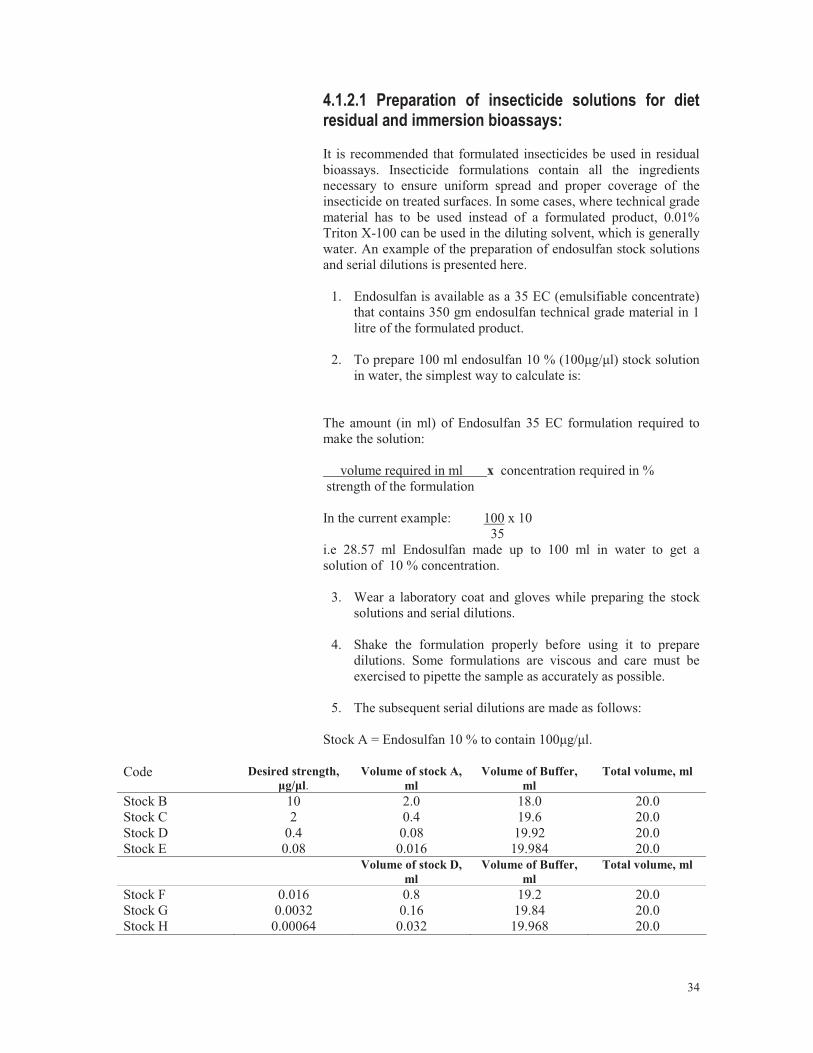
4.1.2.1 Preparation of insecticide solutions for diet residual and immersion bioassays: It is recommended that formulated insecticides be used in residual bioassays. Insecticide formulations contain all the ingredients necessary to ensure uniform spread and proper coverage of the insecticide on treated surfaces. In some cases, where technical grade material has to be used instead of a formulated product, 0.01% Triton X-100 can be used in the diluting solvent, which is generally water. An example of the preparation of endosulfan stock solutions and serial dilutions is presented here.

1. Endosulfan is available as a 35 EC (emulsifiable concentrate) that contains 350 gm endosulfan technical grade material in 1 litre of the formulated product.

2. To prepare 100 ml endosulfan 10 % (100μg/μl) stock solution

in water, the simplest way to calculate is: The amount (in ml) of Endosulfan 35 EC formulation required to make the solution: volume required in ml x concentration required in % strength of the formulation In the current example: 100 x 10 35 i.e 28.57 ml Endosulfan made up to 100 ml in water to get a solution of 10 % concentration.

3. Wear a laboratory coat and gloves while preparing the stock solutions and serial dilutions.

4. Shake the formulation properly before using it to prepare

dilutions. Some formulations are viscous and care must be exercised to pipette the sample as accurately as possible.

5. The subsequent serial dilutions are made as follows:

Stock A = Endosulfan 10 % to contain 100μg/μl.

Code Desired strength, μg/μl.

Volume of stock A, ml

Volume of Buffer, ml

Total volume, ml

Stock B 10 2.0 18.0 20.0 Stock C 2 0.4 19.6 20.0 Stock D 0.4 0.08 19.92 20.0 Stock E 0.08 0.016 19.984 20.0 Volume of stock D,

ml Volume of Buffer,

ml Total volume, ml

Stock F 0.016 0.8 19.2 20.0 Stock G 0.0032 0.16 19.84 20.0 Stock H 0.00064 0.032 19.968 20.0

35

4.1.3 Surface coating/ residual bioassays. 1. For bioassays with leaf feeding insects, it is recommended that

the assays be conducted with leaves of the most popular, commonly grown host plant variety.

2. We commonly use plastic cups with inner dimensions of 6.8 x

5 (d x h) for the cotton leaf disc residue bioassays.

3. Add 1 gm agar to 99 ml water and disperse the agar properly by constant stirring. Heat the solution until it boils. Allow it to cool to 650C. Add 0.3 ml of anti-mould solution. Vortex and pour the solution into the plastic cups to get a 0.5 cm thick layer. Add 4.5 ml phosphoric acid and 42 ml propionic acid to 53.5 ml water to make the anti mould solution.

4. Tender cotton leaves are washed under tap water, and

sandwiched gently in blotting paper to remove the water. Leaf discs of 6.5 cm diameter are punched out from the leaves using a metal lid. The discs are coated with 100 �l of the diluted toxin on each side and air-dried. The toxin can be gently spread on the leaf using the bottom side of a test tube, 0.5 x 5 cm d x h.

5. Place the toxin-coated discs on the agar layer and release one,

second instar or 10 first instar, H. armigera larvae per cup. Always maintain proper controls with untreated leaf discs.

6. Close the cups with finely perforated lids and transfer the cups

to bioassay chambers with 25 + 1oC, 70 + 5 R. H or to BOD incubators.

7. Change the leaves at least every alternate day, preferably

everyday.

8. Record mortality for seven days, and individual weights of surviving larvae on the seventh day.

36

4.1.4 IRAC Methods The following methods have been developed by IRAC (Insecticide resistance action committee) and are used extensively by researchers. The three methods being presented here are relevant for cotton pests and can be used with minimum modifications. 4.1.4.1 IRAC Method No. 1

Pest species: Myzus persicae Suitable for organophosphates and carbamates Materials required Petri dishes (9-cm diameter), plastic bags, cotton wool, untreated leaves, small forceps, fine pointed brush or cocktail stick, beakers or glass jars (ca. 100-ml capacity) for test liquids, 1-ml disposable plastic syringes for liquids or balance for solids, hand lens or binocular microscope, maximum/minimum thermometer. Method 1. Sample apterous aphids by collecting infested leaves, selected

at random from several plants. The leaves may be transported and held in plastic bags.

2. Collect some non-infested, untreated, leaves or remove aphids

from leaves using a small brush before treatment.

3. Prepare test liquids. The use of a wetter is not recommended. Agitate test liquids and then dip non-infested leaves for 5 s, five leaves per treatment. Dip five control leaves in water.

4. Allow surface water to dry from leaves before placing them

individually in Petri dishes and infesting each leaf with 20 adult aphids. The aphids can be transferred using a small pointed brush (with volatile insecticides it may be necessary to ventilate the Petri dishes by piercing the lids with a hot wire).

5. Place a small piece of damp cotton wool around the petiole of

each leaf.

6. Store Petri dishes in an area where they are not exposed to direct sunlight or extremes of temperature. Record maximum and minimum temperatures.

7. Using a hand lens or binocular microscope assess mortality

after 24 h by checking the aphid’s ability to show co-ordinated movement in response to a touch with a small brush or cocktail stick.

8. Express results as percentage mortality and correct for

untreated mortality using Abbott’s formula. Untreated mortality should be quoted.

37

4.1.4.2 IRAC Method No. 7 Pest species: leaf-eating larvae of Lepidoptera Including Heliothine species and coleoptera on cotton, vegetable and field crops. Suitable for organophosphates, carbamates, pyrethroids, organochlorines and insect growth regulators Materials required

Insect-proof containers, scissors, forceps, fine pointed brush, beakers for test liquids, syringes/pipettes for liquids or balance for solids, syringes/pipettes for making dilutions, binocular microscope or hand lens, untreated leaves, paper towels, maximum/minimum thermometer.

Method

1. Collect in a field a representative sample of insects. These may be larvae suitable for immediate testing, or eggs/L1 larvae for rearing to the appropriate stage or material from which an F1 population for testing can be reared. The insects should not be subjected to temperature, humidity or starvation stress after collection.

2. Collect sufficient non-infested, untreated leaves. Whole leaves are preferred or, for some crops, the

distal portions. Do not allow leaves to wilt. 3. Prepare accurate dilutions of the test compound from identified commercial product. For initial

studies, five widely spaced rates are recommended. The use of additional wetter is only recommended for highly waxed leaf material, in which case this wetter solution is used for the ‘untreated‘ (control) solution on place of water alone.

4. Dip leaves individually in the test liquid for 5 s with gentle agitation and place to surface-dry on

paper towelling. Do not allow to wilt. Dip the same number of leaves per treatment, and treat sufficient leaf material to avoid starvation stress in the 'untreated‘ during the test. Commence dipping the ‘untreated‘ first and work up through the test liquids. Place the treated surface-dry leaves in the labelled test containers, which must be suitable for holding enough leaf material in good condition for up to 3 days.

5. Add equal numbers of neonate larvae (Heliothis) or recently molted L2 larvae to each container, so

that a minimum total of 40 larvae are used per treatment, divided between at least four replicate containers. It only one leaf surface is accessible to the larvae, ensure that this is the correct one for the species involved. If cannibalism is a problem (e.g. in Heliothis), reduce the number or larvae per container but increase the replication.

6. Store the containers in an area where they are not exposed to direct sunlight or extremes of

temperature. Record maximum and minimum temperatures. If possible a mean temperature of 25°C is preferred.

7. In the case of rapidly acting compounds, a final assessment of larval mortalities is made after 48 h.

For slowly acting compounds (e.g. benzoylureas, insect growth regulators etc.) a first assessment is made at 72 h, when the leaves are changed for fresh leaves treated, as before, with the appropriate insecticide dilution. The containers are held for a further period before the final assessment, either for 72 h or until larvae in the ‘untreated‘ (control) have moulted again.

8. Express results as percentage mortalities, correcting for untreated (control) mortalities using

Abbott’s formula. Untreated mortality should be quoted.

38

4.1.4.3 IRAC Method No. 8

Pest species: Bemisia tabaci (adults) Materials required Clean plastic cups with push-on plastic lids, plasticine, nylon muslin with very small mesh (approximately 10.000 apertures cm-2) sharp knife or scalpel, scissors, glue, nail or other similar metal rod, untreated leaves. Method 1. Turn a plastic lid upside down and cut a circular hole

(approximately 4 cm diameter) with a scalpel. Cut a roughly circular piece if muslin (approximately 5.5 cm diameter) and glue to the inside of the prepared plastic lid. Heat the nail (or metal rod) and pierce a hole in the bottom of the plastic cup.

2. Select uncontaminated cotton leaves and with scissors cut the

petiole to a length of approximately 4 cm. Cut the lamina to give an approximately square area (2 x 2 cm). Prepare a minimum of four replicates per treatment.

3. Prepare test liquids. The use of a wetter is not recommended.

Agitate test liquids and then dip prepared leaves for 5 s holding the leaf by the petiole. Leave the leaves to dry in the open air (approximately 5 min).

4. Pass the petiole of a test leaf through the hole in the plastic cup

until it protrudes by approximately 1 cm. Fix the petiole in position by pressing a small ball of plasticine around the petiole where it enters the cut hole.

5. Take the cup to an infested cotton plant and with the lid on the

upper surface of an infested leaf move the cup upwards onto the underleaf surface. Move the lid and cup together sideways off the leaf to trap the adult whiteflies. Repeat procedure until approximately 50 adults per cup have been collected. Place a small amount of water in a second plastic cup and stand the test cup inside this so that it is supported by the protruding petiole.

6. Record number of adults per cup. The whiteflies will settle in

the cut leaf.

7. Hold containers, in constant conditions wherever possible, for 48 h. Extremes of temperature should be avoided, 25°C is preferred. Containers must not be exposed to direct sunlight. Record living and dead whiteflies after 48 h.

8. Express results as percentage mortality and correct for

untreated mortality using Abbott’s formula. Untreated mortality should be quoted.

Possible problems

The test chambers must be very dry as whiteflies die if they get caught up in water.

Some of the insects become stuck to the surface of the test chamber because of the static charge present. If the compound under test has repellent properties, the whiteflies will not settle on the test leaf and this may affect mortality.

39

4.1.5 Immersion methods Larval dip and immersion of small-bodied insects in insecticide solutions are convenient field based bioassays useful for extension and field workers. The methods are simple and are somewhat closer to field application of insecticides. However, many extraneous factors and practical problems make the assays unreliable under some conditions. For example, it is not very easy to collect adequate sample sizes of 100-200, healthy third instar larvae from fields in a short period of time unless there is a very heavy infestation that goes beyond economic threshold levels (ETL). And when pest populations are at ETL stage, farmers rarely wait for bioassay results before making pest management decisions. Field collected third instar H. armigera larvae are rarely healthy. Most of them harbor diseases and parasitoids. Third instar H. armigera larvae are cannibalistic and hurt one another when in proximity. They must be collected and kept in separate cells. When they have to be dipped, it is important to ensure that they are not dipped in groups. In a group they get entangled, cling together and start biting each other. Therefore, larvae have to be dipped one at a time, placed on blotting paper to remove excess insecticide and then placed on diet in individual wells of multi-cell trays. The following protocol is useful for H. armigera. 1. Collect at least 150 third instar H. armigera larvae directly

from fields and place larvae singly in individual cups.

2. Sort out 30-40 mg larvae. Discard underweight and overweight larvae.

3. Ideally, the recommended field application rate should set a

proper guideline for the assay. For example, if endosulfan 35 EC is recommended for field application at a concentration of 0.07 %, then the calculations is as follows

Formulated compound required = Recommended concentration x Final volume to be used Strength of the formulation In this example: 0.07 x 500 = 1.0 35 i.e 1 ml endosulfan 35 EC made up to 500 ml with water. 4. Dip the larvae one by one and place them on a blotting paper

for a few seconds. Treat at least 100 larvae with the recommended dose. Keep 20-30 untreated larvae as controls.

5. Replace the larvae on the diet singly in individual wells of

multi-cell trays. Pre-soaked grains of Kabuli-gram (hybrid chickpea) can be used instead of semi-synthetic diet. Change the diet daily.

6. Record observations every day for 4 days.

40

7. Discard diseased and parasitized larvae. Do not include their numbers in the final calculations.

8. Calculate % mortality as follows:

Corrected mortality = (% mortality in treatment - % mortality in control) x 100 (100 - % mortality in control) Acceptable insecticide efficacy levels depend on the pest population intensity, economic thresholds for the pest, damage potential, cost of the insecticide application and value of the agricultural produce. Use the mortality data to assess how much value a pesticide application would add to the economic returns by preventing damage to the produce and then decide on the course of action. When pest population is at ETL levels, larval mortality of < 80 % is generally unacceptable by farmers. 4.1.6 Sticky card assay The sticky card test (Prabhaker, et al., 1988) has been extensively used to monitor insecticide resistance in whiteflies. The test is simple and elegant and has the advantage of being easily used by field workers.

1. Yellow cards (7.5 x 12.5 cm) are sprayed with a thin layer of sticky adhesive using aerosol can.

2. Serial dilutions of formulated insecticides are sprayed on the

cards using Potter’s tower.

3. Controls are sprayed with water.

4. Treated cards are carried to the field in cool boxes and exposed to whiteflies for a fixed period of time, generally one or two minutes.

5. The cards are placed on styrofoam slabs at room temperature

in humid conditions.

6. Mortality observations are recorded 24 h later. The test has advantages over the vial method. Insecticide used in vial tests were found to degrade more rapidly in vials compared to on the sticky cards. Unlike the vial tests, the sticky card test does not impose a fumigation effect and does not provide untreated areas for insects to seek refuge.

41

4.1.7 Diet incorporation methods for oral toxicants Diet incorporation or diet coating methods, are used to assess the effects of insect growth regulating compounds and oral toxicants on active feeding stages of insects. In-planta bioassays are used to evaluate the effects of systemic insecticides on sap sucking insects and to assess the efficacy of toxin-producing transgenic plants on target insects. The assays being described here focus mainly on Cry toxins, but can be used with slight modifications for any oral toxicants such as insect growth regulators or stomach poison insecticides. 4.1.7.1 Preparation of Cry1Ac toxin solutions for bioassays Bacillus thuringiensis (Bt) is a gram positive soil inhabiting microorganism. It produces a proteinaceous crystal toxin that is toxic to many insect pests especially lepidopteran larvae. The main types are the Cry (crystal) toxins, encoded by different cry genes, the second type the Cyt (cytolytic) toxins, which can augment the Cry toxins, enhancing the effectiveness of insect control and the third VIP (vegetative insecticidal proteins) toxins, which are produced during vegetative phase. B. thuringiensis are known to produce 181 toxins. The genes that encode these toxins have now been sequenced and enable the toxins to be assigned to more than 46 groups of Cry toxins (Cry1 to Cry46), 2 groups of cytolytic toxins (Cyt1 and Cyt2) and 3 groups of VIP toxins (VIP1 to VIP3), on the basis of amino acid sequence similarities. The table below shows a brief classification of the toxins. The Genes encoding several toxin crystal (Cry) proteins have been cloned (Albert et al., 1990) in the hyper-expressing recombinant plasmid vector pKK 223-3 into Escherichia coli to produce isolated Cry toxins constituting 40 % of the total soluble protein produced by the bacteria. Cry1Ac, which is the most toxic of all the Cry toxins to H. armigera is also available as a recombinant product in a commercial formulation called MVP-II. MVP-II is a lyophilized form of a liquid formulation containing 19.7% Cry1Ac encapsulated in Pseudomonas fluorescens. The Cry1Ac in MVP-II is 99% identical to the active toxin region of the Cry1Ac expressed in Bt cotton.

Features of the Cry toxins

Protein Crystal shape Size (kDa) Insect activity

Cry 1 [41 toxins, Aa to La] bipyramidal 130-135 lepidoptera Cry 2 [5 toxins, Aa to Ae] cuboidal 70 lepidoptera and diptera Cry 3 [4 toxins, Aa to Ca] flat/irregular 74 coleoptera Cry 4 [2 toxins, Aa & Ba] bipyramidal 70-133 diptera Cry 5-46 [85 toxins] multiple 33-130 Un-defined

42

4.1.7.2 Preparation of Cry toxins from recombinant clones 1. Cry1Ac toxins are produced from E. coli clones expressing

Cry1Ac. The toxins isolated from sonicated cells. The recombinant E. coli cells are grown in sterile Luria broth, pH 7.5, containing 1 % each of sodium chloride and tryptone and 0.5 % yeast. Inoculate 2ml of Luria broth (containing an appropriate antibiotic) with a single cell colony of the recombinant E. coli harbouring the Bt gene. Grow overnight at 370C with constant shaking. Take a wire loop full of bacterial culture and inoculate 250 ml Luria broth. Shake the flasks constantly for 48h at 370C.

2. Centrifuge the bacterial culture at 10,000rpm, 40C, for 20 min.

The pellet contains bacterial cells. Re-suspend the pellet in 60 ml of 50 mM Tris pH 8.0 containing 50 mM EDTA, 15 % sucrose and 0.05 % lysozyme. Incubate at room temperature with slow shaking. Centrifuge and re-suspend the pellet in 60 ml buffer containing 0.5 M NaCl, 2 % Triton X-100.

3. Sonicate the sample in an ice bath, for 10 minutes with an

interval of 1min after 5min.

4. Add 60ml of buffer containing 0.5 M NaCl, 2 % Triton X-100, and centrifuge at 10,000 rpm, 4oC, for 20min.

5. Wash the pellet three times with 10 % sodium bromide, twice

with 0.5 M NaCl and finally three times with sterile water. The pellet can be suspended in distilled water and used for bioassays directly. Cry1Ac in the sample can be estimated from an aliquot drawn separately. Cry1Ac in MVP formulation is pre-quantified, and can be used directly for bioassays.

6. Centrifuge the sample. Re-suspend the pellet in 5 ml

solubilization buffer pH 9.5, containing 50 mM sodium carbonate and 10 mM DTT (dithiothreitol). Incubate the sample for 3 - 4 h with slow shaking at 37oC. Centrifuge the sample at 10,000 rpm for 10 min. The supernatant contains solubilized Cry1Ac protoxin.

7. Estimate protein in the supernatant by Lowry’s method (Lowry

et. al. 1951) and Cry1Ac content by ELISA. The Cry1Ac content can also be estimated by densitometry on SDS-PAGE gels using standard pre-quantified markers.

8. MVP formulation can be diluted in buffer containing 50 mM

Tris pH 8.0 containing 50 mM EDTA, 15 % sucrose and 0.05 % lysozyme and processed in exactly the same way as used for the Cry1Ac toxin isolation to obtain solubilized protoxins.

9. After solubilization, the protoxins become relatively unstable

in prolonged refrigerated storage. Hence, it is recommended that the toxins be used for bioassays immediately after solubilization.

43

4.1.7.3 Diet incorporation Serial dilutions of the toxins are made as follows. If the toxins are to be used in leaf surface coating assays, add Tween-20 to a final concentration of 0.01 % in the dilution buffer. Stock A = 40 μg/ml

Code Desired strength ,μg/ml

Volume of stock A, ml

Volume of Buffer ml

Total volume ml

Stock B 10 5.0 15.0 20.0 Stock C 2 1.0 19.0 20.0 Stock D 0.4 0.2 19.8 20.0 Stock E 0.08 0.04 19.96 20.0 Volume of

stock D, ml Volume of Buffer

ml Total volume

ml Stock F 0.016 0.8 19.2 20.0 Stock G 0.0032 0.16 19.84 20.0 Stock H 0.00064 0.032 19.968 20.0 The following protocol is used for diet incorporation of oral toxicants to test their toxicity on target insects. The example presented here is to bioassay Cry1Ac on H. armigera. 1. Pipette out 3 ml of the solution into a 40 ml plastic cup.

2. Pour lukewarm diet, approx 60o C, into the cup to a total

volume of 30 ml. Place the lid and shake the cup vigorously for a minute to mix properly.

3. Pour the diet to 0.5 cm height, into wells of a 24-cell insect-

rearing tray. Allow the diet to cool in laminar airflow under UV lamps for 1 h to surface sterilize the diet.

4. If concentration of the toxicant in the stock solution was 2

μg/ml, the final concentration in the diet would now be 0.2 μg/ml diet. Thus the final concentration of toxin in diet was diluted 10-fold.

5. Release first instars into the diet rearing trays at the rate of one

per well. Cover the diet tray with semi-permeable wrap and close the lid.

6. It is recommended that the lid be tightly secured to the tray

with rubber bands, to prevent the larvae from escaping. Because the diet is unsuitable, larvae try constantly to escape from the diet rearing trays.

7. Keep controls with larvae released on untreated diet, for all the

experiments.

8. The unused rearing trays with diet can be stored in a refrigerator for a week.

9. Change the diet for the larvae every two or three days.

44

10. Record mortality observations at 8 hourly intervals until the end

of seven days, for median lethal time LT50 calculations. LT50 is the time at which 50 % of the test population is killed with the specific dose tested. A simple linear regression equation can be worked out to calculate the LT50.

11. Otherwise, record mortality at alternate days until the end of

seven days, for median lethal concentration LC50 calculations. LC50 is the concentration that kills half the test population.

12. Record weights of surviving larvae at the end of seven days, for

median effective concentration EC50 and IC50. EC50 is the concentration that prevents half the test population from reaching 50 % of the weight attained by control larvae. For example if the average weight of larvae on the control diet (without toxin) was 80 mg, EC50 represents the concentration at which 50 % of the test population is unable to gain a weight more than 40 mg. IC50 is the concentration that prevents half the test population from reaching the third instar.

4.1.7.4 Diet incorporation for filter paper bioassays 1. For bioassays with bollworms, 10 ml toxin incorporated diet is

poured over a 16 sq cm piece of filter paper. The filter papers layered with diet are cooled and cut into smaller squares of 2 x 2 cm, and 10 first instar larvae are released in small plastic cups 3 x 3 cm (d x h) cups containing a square. Change the strips every alternate day.

2. Record mortality observations until the seventh day. 4.1.7.5 Surface coating of semi-synthetic diet 1. Pipette out 25 �l of the toxin solution into each well of the 24-cell insect-rearing tray. Generally 10 �l of the toxin can be used to coat 1 sq cm surface area. Gently swirl the trays to ensure uniform and complete spread of the solution over the diet surface. 2. Allow the surface to dry in a laminar airflow under UV light for 2-3 h to surface sterilize. 3. Release one, first instar H. armigera larva per well. Always maintain proper controls with untreated diet. 4. Change the diet on alternate days and record mortality until the seventh day. Then, weight of surviving larvae should be recorded on the final day of the bioassay. The method has the advantage of obtaining constantly reliable results because the toxin is unlikely to be affected by either improper mixing or heat as can occur in the diet-incorporation method. Moreover, less amount of the toxin is required for the assay, compared to the diet-incorporation method.

45

Chapter 5 Bioassays with transgenic plants Transgenic Bt-cottons currently express Cry toxins. The toxins are effective in causing mortality to a wide range of cotton pests. However, resistance development in target pests can impair the toxic effects. Bioassays with transgenic plants help in 1. Evaluating efficacy of the plants on target pests. 2. Determining the expression levels of the Cry toxins. 3. Confirming resistance when it occurs in target pests. Several bioassays can be used to evaluate the efficacy and determine the expression levels. Some of the standard methods are given below. When the main objective is to determine the expression levels of Cry1Ac in Bt-cotton plants, it is necessary to set up standard curves with the matrix of the plant parts being tested for expression.

5.1 Bioefficacy of Bt-transgenic plant parts 1. The Bt-cotton plant parts to be tested are excised along with

their petiole from the node, and brought to the lab in cool boxes. The plant parts are rinsed under tap water and sandwiched gently in two layers of blotting paper to remove the water.

2. The bioassay is carried out in cups having a 3 mm diameter

hole at the bottom, through which the petiole is passed and the distal end dipped in 0.5 % agar, containing anti-mould solution and Murashige-Skoog medium (optional), present in a cup held beneath the upper cup. The hole is plugged with wax around the petiole. Alternatively, the plant parts are placed in plastic cups directly or on a moist layer of blotting paper. However, in this case, the parts will have to be changed everyday, to avoid larval mortality or growth reduction due to tissue deterioration.

3. Ensure that the same method of bioassay is followed to

generate standard curves with plant parts from non-Bt plants and to test the efficacy of the plant parts from Bt-cotton.

4. Release five, first instar larvae on the plant part in each cup.

Close the cups with finely perforated lids and transfer the cups to bioassay chambers or to BOD incubators at 25 + 1oC, 70 + 5 % R. H. Change the plant parts every alternate day.

5. If the larvae moult to the second instar, transfer each larva into

a single cup, to avoid cannibalism.

6. Record mortality for seven days, and individual weights of surviving larvae on the seventh day.

46

5.2 Whole-plant efficacy assessment Bt-transgenic plants can be tested for their efficacy in no-choice bioassays by confining larvae with plant parts. 1. The simplest of these tests is to release 10 first instar larvae on

each branch (sympodia of cotton plants) and cover them with two layers of fine-perforated plastic bags.

2. The bags are sealed at the base of the branch tightly with

rubber bands and tape. The bags must be transparent and allow air, but not permit larval escape. Two layers of the bags normally prevent escapes.

3. The method can be used for potted and field grown plants.

4. Observations for the presence or escape of larvae must be

made everyday.

5. Control plants comprise isogenic non-Bt plants on which larva are released and confined in perforated bags, identical to that on the Bt-plants.

6. Final observations are recorded on the seventh day.

7. The reduction in weight of larvae surviving on Bt-plants can be

calculated relative to the average weight of larvae on control plants.

8. Mortality observations can be used to calculate the % mortality

on transgenic plants, in comparison with that on non-Bt plants.

47

5.3 Cry1Ac estimation using bioassays Surface coating or diet incorporation bioassay methods are used to estimate Cry toxin concentration present in Bt-cotton plants. Standard curves are generated using tissue a matrix derived from the corresponding isogenic non-Bt plant parts and testing is done with a tissue matrix prepared from the test Bt-cotton plant parts. 1. Surface coating of intact tissues with standard Cry serial stock

diluted solutions is done to obtain standard curves. The standard curves are generated with plant parts of the corresponding isogenic non-Bt plant variety.

2. Intact non-Bt plant parts such as leaf, bracts, boll rind, petals

etc. are coated with a serial dilution of the Cry toxin solutions containing 0.1 % Triton X-100. Care must be taken to ensure that the age of the plant part tissues is the same as that of those being tested. Conduct the bioassay as described above.

3. Plot linear regression graphs of a). log-dose v/s mortality and

b). log dose vs % weight reduction.

4. Calculate the amount of Cry1Ac present in the tissues, by plotting the mortality or % weight reduction values and reading from the standard curve graph

5. Alternatively, Cry standard curves can be generated using

lyophilized or liquid nitrogen plant tissue powders incorporated or coated on semi synthetic diet. Excise plant parts of the same age from non-Bt plants and the corresponding isogenic Bt plants. Bring them to the lab on ice. Prepare tissue powders from the non-Bt plant parts first and then from Bt plant parts using liquid nitrogen. Some protocols (Sims et al., 1996) suggest that it is better if the tissues are lyophilized and homogenized in dry ice to a fine powder.

6. Store the powders at –80oC in dessicators. Prepare a 10 %

solution of the tissue powder (w/v) in sterile water, freshly before use, by adding 10 g of the powder to 90 ml water containing 0.5 % ascorbic acid.

7. For the standard curve, prepare serial dilutions of the Cry toxin

in the solution of non-Bt plant part tissue powder hereafter referred as serial dilutions of stock X.

48

Preparation of working stock solutions Prepare stock A, as follows: Add 2 g non-Bt powder to a 8 ml stock solution (100μg/ml) Cry toxin solution and make up the volume to 20 ml with water. Stock A = 40 μg /ml Cry1Ac in 10 % solution of isogenic non-Bt-plant powder Stock B = 10 % solution of isogenic non-Bt-plant powder

Code Desired strength, μg/ml

Volume of stock A

ml

Volume of stock B

ml

Total volume Stock X

ml Stock 1 10 5.0 15.0 20.0 Stock 2 2 1.0 19.0 20.0 Stock 3 0.4 0.2 19.8 20.0 Stock 4 0.08 0.04 19.96 20.0 Volume of

stock 3, ml Volume of stock B, ml

Stock 5 0.016 0.8 19.2 20.0 Stock 6 0.0032 0.16 19.84 20.0 Stock 7 0.00064 0.032 19.968 20.0 Stock 8 0 0 20.0 20.0

For log dose probit assay of the test sample, prepare serial dilutions of the test sample as follows: Stock B: 10 % solution of isogenic non-Bt-plant powder Stock C: 10 % solution of Bt-plant powder % Bt-plant powder

Stock B ml

Stock C ml

Stock Y Final volume

10% 0 10 10 6% 4.0 6.0 10 3% 7.0 3.0 10 0.6% 9.4 0.6 10 0.3% 9.7 0.3 10 0.06 % 9.94 0.06 10 0.01% 9.99 0.01 10 0 10 0 10

49

5.4 Log Dose Probit assay For surface coating, pipette out 25 �l of the serial dilutions of stock X or stock Y toxin solutions on the diet surface in each well of the 24-cell insect-rearing tray. Generally 10 �l of the toxin can be used to coat 1 sq cm surface area. Gently swirl the trays to ensure uniform and complete spread of the solution over the diet surface. Allow the surface to dry in laminar airflow under UV light for 2-3 h to surface sterilize. 1. For diet-incorporation, add 24 ml of warm diet (60oC) to 6 ml

of the serial dilutions of stock X or stock Y toxin solutions, vortex for 1 min and pour in a 24-cell multi-cell insect rearing tray. If the concentration of the toxicant in the stock solution X was 2 μg/ml, the final concentration in the diet would now be 0.4 μg/ml diet. Thus the final concentration of toxin in the diet would be diluted by a 5-fold factor

2. Release one, first instar H. armigera larva per well. Always

maintain proper controls with untreated diet.

3. Change the diet on alternate days and record mortality until the seventh day. The weight of surviving larvae should be recorded on the final day of the bioassay.

4. The method has an advantage of obtaining reliable results

because the toxin is unlikely to be affected by either improper mixing or heat as can occur in the diet-incorporation method. Moreover, less amount of the toxin is required for the assay, compared to the diet-incorporation method.

5. Calculate the amount of Cry1Ac present in the tissues, by

plotting the mortality or % weight reduction values and reading from the standard curve graph.

6. Subtract the response (mortality or % weight reduction) of the

non-Bt control from the corresponding Bt-plant treatments. For example if response (mortality or % weight reduction) with stock Y (non-Bt control) was 5 %, then the corrected response using Abbott’s formula would be:

Corrected response = (% response in treatment - % response in control) x 100 (100 - % response in control) 7. Subject the data to log-dose probit analysis.

50

Chapter 6 Statistical analysis of bioassay data

6.1 Statistical analysis of dose-mortality responses Log dose probit analysis is carried out to obtain a regression equation that enables the calculation of the dose / concentration required for any particular % mortality that they cause in the test population. The analysis can also be done for biological responses other than mortality, such as weight reduction, moult inhibition etc. For the regression analysis, it is necessary to assess the biological response of the organism against a series of serially diluted concentrations. Once the bioassay results are found to confirm to a graded response depending on the concentration of the toxicant, they are then subjected to probit analysis through a series of manual calculations or on computer-aided programs such as POLO, MLP, MSTAT, GENSTAT etc. The details of probit analysis are not being dealt with here. Generally the median lethal dose (commonly called the LD50, a dose which kills 50% of the test population) is calculated to compare responses of test populations. If control mortality exceeds 5% discard the replicate. 1. Use Abbott’s formula to correct control mortality % Test mortality - % control mortality x 100 100 - % control mortality 2. Plot percentage mortality on a probit scale against log

insecticide dose. Read the LD50 and LD90 values from the graph. Alternatively software programs such as POLO-PC, MLP, MSTAT, GLIM or GENSTAT may be used for probit analysis. Resistance factors (RF) or resistance ratios (RR) can be calculated if data for the response of a susceptible strain is available.

RF = LD50 of test strain LD50 of the susceptible strain The comparison would be valid only if the regression lines of the susceptible and resistant strains are parallel. However, this is generally not the case and hence may not justify valid comparisons between populations with differing slopes due to genetic variability. Robertson and Preisler, 1992, proposed a method to derive resistance ratios, which includes LDx and slope data of both the populations being compared. The method is being presented below. Because simple lethal dose ratios do not provide any estimate of the error involved in the calculation, the most practical and least restrictive alternative is to estimate 95% confidence limits for each ratio. Based on estimates for the intercepts (αi, i = 1,2) and the slopes (εi, i = 1,2) of two probit (or logit) lines and estimates of

51

their variance-covariance matrices, all of which are produced in the POLO-PC output, the confidence limits for the ratio is calculated by the following steps: Example: POLO OUTPUT –Susceptible strain

POLO OUTPUT –Resistant strain

52

1. For i = 1,2 calculate Ǿi = Xπ - άi έi Where Xπ is the πth percentile point of the probit (or logit) distribution curve. Values of Xπ for comparing LD50, LD90 and LD99 are 0, 1.28 and 2.33 respectively. 2. Calculate var(Ǿi) = 1/ έi

2 [var(άi) + 2Ǿi cov(άi έi) + Ǿi2 var(έi )]

3. Calculate a = Ǿ1 - Ǿ2 and σ = � var(Ǿ1) + var(Ǿ2) 4. Estimate of the ratio of two lethal doses and the approximate 95% confidence limits are given by ratio = 10a lower limit= 10a-2 σ upper limit = 10a+2 σ Values required to calculate the 95% confidence limits for the LD50 ratio Susceptible Resistant X50 0 0 άi 2.039 0.752 έi 0.819 0.872 var(άi) 0.097 0.0562 var(έi ) 0.012 0.0227 cov(άi έi) 0.0309 0.0273 LD50 0.003 0.137

Step 1. Comparison of LD50 ratios. Calculations for susceptible strain Ǿ1 = 0 – 2.039 = -2.489 0.819 Step 2. var(Ǿ1) = . 1 .[0.097 + 2x (-2.489)(0.0309) + (-2.489 x –2.489)(0.012)] (0.819 x 0.819) = 0.02612 Step 3. Calculations for resistant strain Ǿ2 = 0 – 0.752 = -0.86239 0.872

53

var(Ǿ2) = . 1 .[0.056 + 2x (-0.862)(0.0273) + (-0.862 x –0.862)(0.022)] (0.872 x 0.872) = 0.03418 step 4. Calculate a = Ǿ2 - Ǿ1 = -0.86239 – 2.489 = 1.627 σ = SQRT( 0.0261 + 0.03418) = 0.3989 4. Estimate of the ratio of two lethal doses and the approximate 95% confidence limits are given by ratio = 10a = 101.627 = 42.209 lower limit= 10a-2 σ = 101.627-0.7978 = 6.735 upper limit = 10a+2 σ = 101.627+0.7978 = 264.52 The resistance ratio (95% FL) = 42.2 (6.73 – 264.5)

6.2 Statistical analysis of diagnostic dose data Resistance frequency p = (1- d/n), where d is the number of larvae killed and n is the total number of larvae dosed. The binomial standard error of p is calculated as follows

� p (1 – p) n -1

% Resistance (R) = Resistance frequency x 100. The binomial standard error of % resistance is calculated as follows

� R (100 – R) n -1

The binomial standard error between sites is calculated as follows

� Σ[N x ni2 (pi –p)2 (N –1)n2

Where, pi = proportion of larvae surviving the discriminating dose at site i; ni = total number of larvae tested at site i; N = number of sites (Sawicki et al., 1989). Determine the significance of differences between treatments by the Student’s t-test (Snedecor and Cochran, 1989.)

54

Chapter 7 Synergism studies Synergists are defined as compounds that greatly enhance the toxicity of an insecticide, although they are practically non-toxic by themselves. Thus, when non-toxic compounds contribute to the enhancement in toxicity of insecticides, they are termed synergists. Many chemical compounds have the potential to synergise toxins. Some enzyme inhibitors act as good synergists act by blocking enzymes that detoxify insecticides, especially in insecticide resistant strains. However, some insecticides also enhance the toxicity of other insecticides at non-toxic doses when used in mixtures. When a mixture is more toxic than expected from the sum of their individual efficacies when applied alone, the interaction among ingredients is called synergistic. Antagonistic interactions among components cause the potency of a mixture to be less than expected (Tabashnik, 1992).

Synergism can also occur between two or more toxins. Several statistical methods have been described to quantify synergism of non-toxic as well as toxic compounds. Bioassays to assess toxin interactions are carried out by mixing the toxicants (two or more) in a particular ratio. Serial dilutions are prepared with the mixture. Alternatively the toxins can be administered separately in a sequence in the same proportions as that in the mixture. Bioassays are also conducted to determine the regression dose-mortality response of each of the toxins independently on the same insect strain. The data are subjected to probit analysis and the following statistical methods can be used to evaluate the toxin interactions. The following is a short list of enzyme inhibitors commonly used to synergise toxicity of certain insecticides in resistant insect strains and which thus act as useful indicators of metabolic mechanisms of resistance.

Inhibitor Enzyme systems Reference Piperonylbutoxide (PBO) Mixed function oxidases Chadwick, 1963 Sesamex Mixed function oxidases Beroza and Barthel, 1957 Propargloxypthalimide (PGP) Mixed function oxidases Casida, 1970 1,2,4-trichloro-3-propynyloxybenzene (TCPB) Mixed function oxidases Casida, 1970 Triphenyl phosphate (TPP) Hydrolase Casida, 1970 s,s,s-tributylphosphoro-trithioate (DEF) Hydrolase Casida, 1970 Diethyl maleate (DEM) Glutathione S-transferase Motoyama et al., 1990 4-4’-dichloro-α-methylbenzhydrol (DMC) DDTase Casida, 1970

55

7.1 Evaluating sysnergistic ratios Chou and Talalay, 1984 described methods to derive a combination index (CI) that is useful to determine the additive, synergistic or antagonistic relationship of components in a mixture. CIx = LDx a(m) + LDx b(m) + LDx a(m) LDx b(m) LDx

a LDxb LDx

a LDxb

Where, LDx

a(m) and LDxb(m) are doses of toxicants ‘a’ and ‘b’ used in

the mixture that resulted in mortality x. LDxa LDx

b are lethal doses of toxicants ‘a’ and ‘b’ required to produce mortality ‘x’ when used alone. The combination index value is ‘1’ if the two insecticides show an additive effect, and ≤1 if synergistic, ≥ 1 if antagonistic. For example: If the LD50 of a pyrethroid was 0.35 and 0.42 for an OP compound, the mixture can be categorized as synergistic (CI = 0.74) if the pyrethroids and OP were used at 0.1 + 0.15 in the mixture; additive (CI = 1.0) if their dose was at 0.14 + 0.18; and antagonistic (CI = 1.69) if it was 0.2 + 0.3. Tabashnik, 1992, proposed the following simple similar-action model to evaluate synergism among toxins with similar modes of action. Expected LD50(m) = [ ra / LD50(a) + rb / LD50(b) + rc / LD50(c) ]-1 Where a, b and c are components of the mixture; LD50(m) is the median lethal dose of the mixture; ra, rb and rc are relative proportions of a, b and c used in the mixture and LD50(a), LD50(b) and LD50(c) are the median lethal doses of a, b and c respectively. The expected LD50 thus obtained is then compared with the observed LD50 value to examine if it falls within the 95% confidence intervals. If the expected LD50 is more than the upper limit, the toxins are synergistic and if it is less than the lower limit, the toxins are antagonistic. For example: The LD50 of a pyrethroid was 0.35 and 0.42 for an OP compound and the two toxins were used in relative proportions of 0.4 and 0.6 respectively in the mixture, resulting in an LD50 (95% FL) of 0.25 (0.14 – 0.42). The expected LD50 0.388 falls in the range of fiducial limits and hence the mixture is not synergistic, it may be additive. Note that the equations by Chou and Talalay suggest synergism for the same data! Synergists are very useful in elucidating resistance mechanisms, especially if they are specific inhibitors of a particular resistance-conferring mechanism such as a detoxification enzyme. The compound is used at a non-toxic dose in combination with serial dilutions of the insecticide to assess the toxicity changes in susceptible and resistant strains. LD50s of the insecticide alone and in combination with the synergist on the susceptible and resistant strains are obtained from the bioassay data. Evidence for enhanced metabolic detoxification becomes clear if the synergist has a

56

marginal effect on the toxicity of the insecticide in susceptible strains, but plays a significant role in enhancing toxicity on the resistant strain to a greater extent. The mechanism of resistance is then deduced based on the enzyme-inhibition characteristics of the synergist. For example, if sesamex in combination with cypermethrin on a pyrethroids resistant strain results in LD50 values that are close to that of the susceptible strain, it is inferred that resistance is mediated by monooxygenases, because sesamex is a specific inhibitor of the cytochrome P450 group of monooxygenases. Some representative data are presented below. The effectiveness of a synergist in overcoming resistance mechanisms is represented by synergist ratio ‘SR’ = LD50r LD50r

+x Where LD50r

+x is the LD50 of the insecticide + synergist ‘x’ of resistant strain and LD50r is the LD50 of the insecticide on the resistant strain. When a synergist is used at a fixed non-toxic dose in bioassays with an insecticide to derive LD50 values, synergism is calculated as follows: % Synergism ‘Sy’ = LD50s x 100 LD50r

+x Where LD50r

+x is the LD50 of the insecticide + synergist ‘x’ of resistant strain and LD50s is the LD50 of the insecticide on the susceptible strain. Interpretation of result produced with a diagnostic dose is simpler. The diagnostic dose is used in combination with a fixed non-toxic dose of the synergist. The increase in mortality due to the synergist is calculated and represents synergism. For example if the mortality with cypermethrin 0.1 μg is 24 % and 88 % with cypermethrin 0.1 μg + PBO 20.0 μg, the synergism is 88 – 24 = 64 %. However, the above methods overestimate synergism due to inhibition of resistance-associated enzymes, because they do not take into account the extent of synergism in the susceptible strain. From a practical perspective, it may not matter much because it still indicates the levels of insecticide toxicity enhancement by the synergist in a resistant strain in comparison to the toxicity of the insecticide on a susceptible strain. The actual resistance related synergism is calculated as follows: % Actual resistance related synergism ‘Sr’ = LD50s +x x 100 LD50r

+x Wherein LD50r

+x is the LD50 of the insecticide + synergist ‘x’ of resistant strain and LD50s

+x is the LD50 of the insecticide + synergist ‘x’ of the susceptible strain.

57

Chapter 8 Metabolic resistance mechanisms Insecticide Resistance: Resistance is “the inherited ability of a strain of some organism to survive doses of a toxicant that would kill the majority of individuals in a normal population of the same species” (WHO, 1957). Resistance in insects is usually a complex phenomenon with more than one mechanism operating simultaneously within the same insect strain (Oppenoorth, F. and Welling, W., 1976). Insect resistance to insecticides has been found to be mediated by the following mechanisms: 1. Enhanced enzymatic metabolism

i. Microsomal mono-oxygenases ii. Phosphotriester hydrolases

iii. Carboxylesterases iv. Glutathione S-transferases v. DDT-dehydrochlorinases.

2. Altered target site sensitivity i. Insensitive acetylcholinesterases

ii. Insensitive sodium channels iii. Insensitive GABA (γ-amino butyric acid) receptor

3. Penetration resistance 4. Altered behavioural patterns

58

8.1 Enzyme classification The International Union of Biochemistry and Molecular Biology (IUBMB) defined six major classes of enzymes based on the reactions they catalyze. Further, the nomenclature committee also recommended the classification for subclasses and sub-subclasses. Each enzyme is assigned an EC (Enzyme Commission) number. For example, the EC number of carboxylesterase is EC 3.1.1.1. The first digit ‘3’ indicates that the enzyme belongs to hydrolase. Rest of the digits that follow ‘3’ represent subclasses and sub-subclasses.

1. Oxidoreductases

Oxidoreductases catalyze a variety of oxidation-reduction reactions. Some examples of this class are oxidase, reductase, dehydrogenase and catalase.

2. Transferases

Transferases catalyze transfers of chemical groups such as methyl, acetyl, phosphate, nucleotides etc. and are called methylase, acetyltransferase, protein kinase and DNA or RNA polymerase respectively. The Glutathione S-transferases of this class have been implicated for their role in conferring insecticide resistance in insects.

3. Hydrolases

Hydrolases catalyze hydrolysis reactions where a molecule is split into two or more smaller molecules by the addition of water. Acetylcholine esterase, carboxylesterase, epoxide hydrolase, and phosphotriesterase are some of the common examples of enzymes under this class that are associated with insecticide resistance in insects.

4. Lyases

Lyases catalyze the cleavage of C-C, C-O, C-S and C-N bonds. These catalytic reactions do not include hydrolysis or oxidation. Common examples under this class are decarboxylase and aldolase.

5. Isomerases

Isomerases catalyze atomic rearrangements within a molecule. Notable examples are epimerase and racemase.

6. Ligases

Ligases catalyze the reaction, which joins two molecules. DNA ligase, RNA ligase, peptide synthase and aminoacyl-tRNA synthetase are some enzymes under this class.

59

8.2 Biochemical routes of insecticide detoxification Insects metabolize insecticides to non toxic or less toxic forms through a process called ‘detoxification’ and sometimes to more toxic intermediates, a process called ‘activation’. Substances that are completely water soluble (polar), and those that are completely insoluble in either water or fats, are excreted unchanged. Most insecticides, which are water insoluble (apolar) or fat soluble (lipophilic), are metabolised to polar compounds through a primary enzymatic conversion, mediated through 1. Oxidases, 2. Hydrolases or 3. Glutathione-S-transferases, resulting in water-soluble products that are subsequently converted to water soluble conjugates through a secondary non synthetic reaction. These conjugates are finally excreted. Apolar substances are converted to less lipophilic or polar metabolites by two reactions (Phase I and Phase II) in insects and many other organisms. Oxidations, reductions and hydrolyses are typical Phase I reactions, which introduce hydrophilic functional groups into apolar molecules to enhance their water solubility. Typically, cytochrome P450 and hydrolase enzymes are involved in Phase I toxin metabolic reactions where they introduce one or more polar groups into substrates and make them suitable for Phase II conjugation reactions. In the Phase II reaction with which the glutathione S-transferases are associated, the Phase I metabolites are conjugated with endogenous intermediates such as water soluble conjugation compounds that are from either carbohydrates, proteins or compounds containing sulphur components. Phase I reactions are mainly carried out by two major groups of enzymes, the oxidoreductases and hydrolases. The oxidoreductases comprise of the cytochrome P450 dependent superfamily of monooxygenases, which introduce oxygen into or remove electrons from their substrates. Carbonyl reductases, alcohol dehydrogenases and aldehyde dehydrogenases remove hydrogen from, or add to the target molecule. The hydrolases hydrolyse esters, amides, epoxides or glucuronides. Typically the Phase I reaction introduces a functional group in a series of steps in lipophilic molecules. The functional groups are divided into two categories. a. Electrophilic substrates. Structures with electrophilic carbon are epoxide functions and α,β-unsaturated carbonyl groups. Some chemically inert molecules (eg. polycyclic aromatic hydrocarbons) are transformed through introduction of electrophilic functional groups, into chemically reactive metabolites, which can react with cellular macromolecules, especially DNA and proteins. However, usually before the electrophiles can react with DNA or proteins, they are rapidly conjugated to the nucleophile glutathione by enzymatic or non-enzymatic conjugation to yield water-soluble molecules.

60

b. Nucleophilic moieties: Alcoholic or phenolic hydroxyl groups, amino and sulphydryl functions or carboxyl groups. Nucleophilic metabolites are generally less harmful than the parent material as they do not covalently interact with endogenous macromolecules such as DNA or proteins. Phase II reactions are mainly carried out by the transferases. Glutathione S-transferases conjugate the electrophilic substrates, while the acetyl transferases, sulfotransferases, acyl-CoA aminoacid N-methyl transferases and UDP-glucuronosyl transferases metabolise the nucleophilic substrates. Insecticide metabolism in insects has been found to be catalysed mainly by monooxygenases, hydrolases and gluthathione S-transferases. Generally in resistant insects, the enzymatic detoxification is believed to be so rapid that the toxic molecule does not reach its site of toxic action.

61

8.3 Mono-oxygenases Mono-oxygenases also referred to as mixed function oxidases, are a group of oxidative enzymes that are localised in microsomes of the endoplasmic reticulum and require NADPH as a co-factor. They are abundant in fat bodies, Malpighian tubules and the midgut of insects. The mono-oxygenases are present in the smooth endoplasmic reticulum, which is a tubular network of lipoprotein that extends throughout the cytoplasm. The enzymes oxidize a range of lipophilic substrates including lipids, steroids and xenobiotics. The mono-oxygenases constitute a number of components of which cytochrome P450 constitutes the terminal oxidases of the system. Cytochrome P450 is a group of hemoproteins, which is the most important since the hemoproteins bind with the substrate as well as with oxygen. The cytochrome P450s are heme-thiolate membrane-bound enzymes present in the endoplasmic reticulum and mitochondria of eukaryotes. They form a complex with the cytochrome P450 reductases in the endoplasmic reticulum. The heme protein links electron flow to the reduction of the oxygen molecule. The cytochrome P450s get their name because of their spectral property of intense absorption of cytochrome-carbon monoxide complex at 450nm. The iron in the mitochondrial cytochrome P450 can functionally assume Fe3+ and Fe2+ forms, whereas the iron in haemoglobin remains in the ferrous state but can coordinate with one oxygen molecule per porphyrin to form oxyhaemoglobin. The mono-oxygenases derive their name because they cause the separation of atoms from oxygen molecules, which end up in different substrates. In the initial Phase of metabolism, oxidized cytochrome P450 binds to the substrate, and gets reduced after receiving an electron from NADPH, mediated by a flavo-protein enzyme NADPH-cytochrome-c-reductase, sometimes stimulated by cytochrome b5. Subsequently an oxygen atom is introduced into the substrate and other combines with hydrogen and forms into water. The oxidation usually results in either epoxidation, hydroxylation, desaturation or dealkylation, or heteroatom oxygenation or replacement of oxygen. In some cases the enzymes act as reductases too. Micosomal hydroxylation of substrate is shown below

62

The general enzymatic process of cytochrome P450 (Estabrook et al., 1971) is briefly described as follows: 1. The ferric form of the cytochrome P450 gets attached to the

substrate -RH. 2. A flavoprotein passes an electron from NADPH to reduce the

complex to the ferrous form. 3. The reduced cytochrome P450-substrate complex gets attached

to molecular oxygen. 4. The bond between the two oxygen atoms is weakened. 5. An intramolecular electron shift leads to the formation of a

peroxide-substrate-RH-ferric P450 complex, and oxide ion and a highly reactive oxygen atom.

6. The oxide ion reacts with a proton to form water and the oxygen atom reacts with the substrate to form an oxidised metabolite R-OH.

RH + NADPH + H+ + 02 ROH + NADP+ +H20 The P450 monooxygenases are known to be extremely versatile in their enzymatic properties. Apart from being involved in endogenous metabolism, they play an important role in detoxification of dietary toxins and exogenously applied insecticides. It is now understood that the mono-oxygenases in insects are involved in conferring resistance to a wide range of insecticides. However, they are also known to activate several molecules, notably the phosphorothioate group of organophosphate insecticides. Mono-oxygenases have been reported to mediate resistance to pyrethroids, DDT, JH mimics, Chitin synthesis inhibitors, carbamates and many organophosphates. In certain resistant strains of Musca domestica, a quantitative increase of cytochrome P450 was found to be due to constitutive over-expression of the gene. But, resistance in many species is also reported due to multiplicity of the cytochrome P450, with some of the isoforms present in the resistant insects exhibiting biochemical and immunological properties different from those in susceptible individuals of the same species. Mono-oxygenase inhibitors have been used to enhance the toxicity of pyrethroids in resistant strains of several insects including H. armigera. Synergism alone or along with enhanced levels of the mono-oxygenases in resistant strains was seen as evidence of the role of mono-oxygenases in pyrethroids resistance. Several enzyme inhibitors were used as synergists to show that specific enzyme classes were involved in resistance. Prominent mono-oxygenase inhibitors amongst these were piperonyl butoxide -PBO (3,4-methylenedioxy-6-propylbenzyl n-butyl diethyleneglycol ether)), Sesamex (2-(3,4-methylenedioxyphenoxy)-3,6,9-trioxaundecane)), safrole (4-allyl- 1,2-methylenedioxybenzene) and isosafrole ((1,2-(methylenedioxy)-4-propenylbenzene)).

63

Oxidation reactions involving mono-oxygenases.

64

Enhanced monooxygenases were implicated in pyrethroid resistance in Australian H. armigera, based on evidence with PBO as a synergist (Forrester et al., 1993). Oxidases and esterases were found to be important mechanisms mediating pyrethroid resistance in H.armigera in India (Kranthi et al. 1997) and Australia (Gunning 1994). Kranthi et al., (2001) reported that enhanced synergism by PBO was positively correlated with high levels of cytochrome P450. Clarke et al. (1990) showed that pyrethroid resistance in H. virescens was largely due to a PBO-synergisable monooxygenase and that the resistant strains possessed a six-fold higher quantity of total cytochrome P450 than the susceptible strain. However, Kennaugh et al. (1993) reported that PBO-suppressible pyrethroid resistance in H. armigera was due to the inhibition of a cytochrome P450-dependent penetration resistance and was not associated with enhanced cytochrome P450 content. Gunning et al. (1998) demonstrated that PBO could also suppress esterase-mediated pyrethroid metabolism in Australian H. armigera strains. Hence, it was argued that PBO-suppressible pyrethroid resistance was not necessarily an indication of cytochrome P450-mediated resistance. Kranthi et al (2001) could not find a positive association between PBO-suppressible pyrethroid resistance and esterase activity in resistant field strains from India. Hence, they inferred that PBO-suppressible resistance indicated the importance of at least cytochrome P450 mediated metabolism in pyrethroid resistant H. armigera strains. They also reported that profenofos-suppressible pyrethroid resistance was positively correlated with esterase activity but the effect was not significant at P�0.05. Apart from cytochrome P450, enhanced levels of P450 reductase and/or b5 have also been found to be associated with insecticide resistance in the sheep blowfly, Lucilia cuprina (Kotze, 1993), Oryzaephilus surinamensis, (Kotze and Wallbank,1996), housefly, Musca domestica (Vincent et al., 1985., Scott and Georghious, 1986), diamond back moth, Plutella xylostella (Sun et al., 1992) and Blattella germanica (Valles and Yu, 1996). While enhanced b5 levels were confirmed to confer resistance in at least Musca domestica (Liu and Scott, 1996), it is still not clear if cytochrome reductase has any significant role to play in mono-oxygenase mediated resistance. Further studies are needed to ascertain the independent and combined roles of each of the three enzymes in insecticide resistance. Cytochrome P450 is a large super family of isoforms consisting of 70 families incorporating 128 subfamilies, with >100 insect P450s alone (Nelson, 1998). The classification of cytochrome P450s is based on sequence homologies, with members within a family sharing >40% and members of a subfamily >55% amino acid homology. All gene members of the cytochrome P450 superfamily are designated with a CYP prefix, followed by a numeral for the family, a letter for the subfamily, and a numeral for the gene (Nelson et al., 1996). Thus far, a total of six (CYP4, 6, 9, 12, 18 and 28) CYP families have been identified in insects. A number of cytochrome P450 genes such as CYP6A1 and CYP6D1 in houseflies, CYP6G1, CYP6A2 and CYP6A9 in Drosophila, and CYP9A1 in Heliothis virescens have been found to overexpress in

65

insecticide resistant strains. But, from the evidence available to date, it appears that only CYP6G1 and CYP6D1 have been conclusively proven to be conferring insecticide resistance in Drosophila and LPR housefly strains respectively (Scott, 1999, Daborn, 2003). At least four cytochrome P450 genes CYP6B2 (Ranasinghe et al., 1997), CYP6B6, CYP6B7 (Ranasinghe and Hobbs, 1998) and CYP4G8 (Pittendrigh et al., 1997) have thus far been implicated in pyrethroid resistance. However, the role of any of these genes in pyrethroid resistance is yet to be definitely demonstrated. The protocols described below represent the measurement of content or oxidase activity of mono-oxygenases, which have been found to be relevant to insecticide resistance and have worked well in our laboratory. The following mono-oxygenase protocols are useful in characterizing resistance in insects: Mono-oxygenase assays 1. Cytochrome P450 and cytochrome P420 2. Cytochrome b5 3. NADPH-cytochrome c reductase 4. Substrate induced spectral changes 5. 7-ethoxycoumarin O-deethylase assay (ECOD) 6. Methoxyresorufin O-demethylase assay (MROD) 7. Ethoxyresorufin O-deethylase assay (EROD) 8. p-nitroanisole O-demethylase assay (PNOD) 9. Benzphetamine N-demethylase assay 10. Peroxidation of tetramethyl benzidine assay 11. Aldrin epoxidase assay. Instruments required 1. Tissue homogeniser 2. Double beam UV-VIS spectrophotometer 3. Spectrofluorometer 4. High speed refrigerated centrifuge 5. Ultra centrifuge Reagents 1. Disodium phosphate 2. Dihydrogen orthophosphate 3. Sodium dithionite 4. Potassium chloride 5. EDTA, (Ethylene diamine tetra acetic acid) 6. PMSF (Phenyl methyl sulfonyl fluoride) 7. PTU (Phenyl thiourea) 8. Glycerol. 9. Potassium hydroxide 10. Sulphuric acid 11. Formic acid

66

Sample preparation for mono-oxygenase assays The mixed function oxidases are present in the microsomal fraction of the endoplasmic reticulum. The microsomal fraction is obtained by differential centrifugation. The cell debris, nuclei and mitochondrial fractions are first removed by centrifuging tissue homogenates at 10,000 X g for 30 min. The pellet is resuspended and centrifuged at 100,000 X g for 2 h to obtain microsomal pellets. Buffers

1. Dissection buffer: Phosphate buffer (100 mM, pH 7.0), containing 1.15% KCl).

2. Homogenization and assay buffer. (prepare fresh): Phosphate

buffer (100 mM, pH 7.0), containing 1mM each of EDTA (ethylene diamine tetra acetic acid), PMSF (phenyl methyl sulfonyl fluoride), PTU (Phenyl thiourea) and 20% glycerol.

Protocol 1. Place a 5th instar larva in dissection tray. Stretch the larva

slightly and pin it down using fine pins, on the dorsal side, through the head and posterior region. Add one ml ice-cold dissection buffer to the dissection tray. Use a sharp razor to make vertical slit all along the dorsal side of the larva. Generally, the slit extends to the dorsal side of the gut making it open up with gut contents seen as a continuous bolus. Remove the food bolus as completely as possible, by pulling it out in a gentle stroke.

2. Scrape off the fat body and food particles.

3. Dissect out the midgut and plunge it immediately into ice-cold

homogenisation buffer (placed in an ice bath). Transfer at least 20 guts to 2 ml fresh homogenisation buffer in a 50 ml polypropylene tube.

4. Place the tube in an ice bucket and homogenise the guts

thoroughly using a motorised homogenizer at 1000 rpm for 45 seconds or more.

5. Add 5 ml of homogenization buffer and centrifuge at 10,000 X

g for 20 minutes at 40C. The supernatant (mentioned henceforth as the enzyme solution) can also be used directly for assays in the absence of ultracentrifugation facilities. If an ultracentrifuge is available, centrifuge the supernatant at 100,000 X g for 4 hours, discard the supernatant and redissolve the microsomal pellet in 7 ml homogenisation buffer.

6. Keep an aliquot of the sample (0.5 to 1 ml) for protein

estimation and use the rest for assay.

67

8.3.1 Cytochrome P450, Cytochrome P420 and Cytochrome b5 assays The cytochrome P450 assay was first described by Omura and Sato (1964) and is a direct method of estimating cytochrome P450 content. Generally, pooled guts of 15-20 fifth instar H. armigera larvae give good yields of microsomal pellets that can be used for the assays with 4 ml cuvettes. The assay volume can also be reduced to 0.5 ml if UV-compatible or quartz microtitre plates are available. Cytochrome P450 Principle: Cytochrome P450 is the only carbon-monoxide binding pigment in the microsomes. In a reduced form it combines with carbon monoxide (CO) to form a complex having an absorption maxima at 450nm when read against its reduced form not treated with CO. The CO difference spectrum of a dithionite-reduced sample is used for determining cytochrome P450 using the extinction co-efficient difference of 91 cm-1 mM-1. Cytochrome b5 Principle: Cytochrome b5 in the reduced condition shows a maximum soret band at 424 nm. The oxidised versus reduced spectrum can be used to calculate the amount of cytochrome b5 using an extinction coefficient of 184 cm-1 mM-1 Protocol 1. Pipette out 3ml of the enzyme solution into each of two 4 ml

quartz cuvettes. Place them in the sample and reference slots of a ‘split beam’ or ‘double beam’ spectrophotometer.

2. Record the baseline from 350 to 500 nm using wave-length

scan mode.

3. Add 5 mg of sodium dithionite to the enzyme in the sample cuvette. Mix well and incubate for 2 minutes at room temperature to reduce the enzyme.

4. Record the spectral change from 350-500 nm in wave-length

scan mode. The data are used to determine the activity of cytochrome b5. The difference in absorbance between measurement at 424 nm and 409 nm (ABS at 424 nm- ABS at 409 nm) can be used to calculate the amount of cytochrome b5, using an extinction co-efficient difference of 184 cm-1 mM-1.

5. To continue with a cytochrome P450 assay, pool the contents

of both cuvettes into a clean test tube. Add 5 mg of sodium dithionite, shake well and incubate for 2 minutes at room temperature.

68

6. Pipette out 3 ml each of the reduced (sodium dithionite treated) enzyme, into the two quartz cuvettes (4 ml) and place one in the reference cuvette slot and the other in the sample cuvette slot of a double beam UV Spectrophotometer. Record the baseline from 400 to 500 nm.

7. Transfer the contents of the sample cuvette into a test tube and

bubble gently with carbon monoxide* for 1-2 mins. Ensure that the tube containing sample solution is covered with aluminium foil, to avoid light. Transfer the contents back into the 4 ml cuvette and place it back in the sample cuvette slot of the spectrophotometer.

8. Adjust the Y axis in the display of the spectrophotometer to 0.4

O.D. Record the difference spectrum from 400 to 500 nm. The difference in absorbance between 450 nm and 490 nm (ABS at 450 nm- ABS at 490) can be used to calculate the cytochrome P450, using an extinction co-efficient difference of 91 cm-1 mM-1. The difference in absorbance between 420 nm and 490 nm (ABS at 420 nm- ABS at 490 nm) can be used to calculate the cytochrome P420 content, using an extinction co-efficient difference of 110 cm-1 mM-1.

69

*Note: Fresh carbon monoxide can be generated by adding 5 ml of formic acid to 10 ml sulphuric acid and passing the gas thus produced through a KOH-dithionite solution, before it is used. Cytochrome b5 (μM) = (ABS at 424- ABS at 409) X 1000 184 Cytochrome P450 (μM) = (ABS at 420-ABS at 490) X 1000 110 Cytochrome P450 (μM) = (ABS at 450-ABS at 490) X 1000 91 Express the cytochrome b5 and cytochrome P450 content per mg protein. Example. Protein concentration of the enzyme solution = 1.5 mg /ml ABS at 450 nm = 0.36, ABS at 490 nm= 0.02, The concentration of cytochrome P450 is calculated as (0.036-0.002) X 1000 = 0.374 μM 91 The cytochrome P450 content would be 0.374 n mol per ml The protein concentration was 1.5 mg/ml. Hence the cytochrome P450 content is expressed as 0.374/ 1.5 = 0.249 n mol /mg protein

70

8.3.1.1.Substrate-induced spectral kinetics of cytochrome P450s Cytochrome P450s are known be present as different isoforms, each with a different substrate specificity, to facilitate detoxification of a wide range of toxicants. The nature of the interactions of cytochrome P450 with substrates is generally revealed through specific spectral changes. Based on the spectroscopic characteristics of the substrate-cytochrome P450 complex, the binding patterns are classified into four major groups as Type-I, Type-II, reverse Type I) and Type-III binding. The cytochrome P450 enzymes carry a heme as the prosthetic group, with an iron as the central atom. In the native state of the enzyme, the iron is in the ferric [ Fe3+] form, predominantly in the low spin configuration in its d5 orbitals. When a substrate molecule binds in the catalytic pocket of the enzyme, it triggers the conversion of iron from a low spin to high spin configuration. This favours the reduction of the ferric [ Fe3+] to the ferrous [ Fe2+] form catalysed by NADPH P450 reductase in a one-electron transfer reaction. In this state, the iron can bind molecular oxygen to form an Fe2+-O2 complex. This complex is further reduced by the NADPH P450 reductase or by the cytochrome b5 that gets activated by the NADPH dependent cytochrome b5 reductase, in a one-electron transfer reaction. The complex thus enters a highly reactive state of Fe2+-O2

- and becomes capable of transferring oxygen to the substrate. Principle: The cytochrome P450 shows a major absorption band at 418 nm in the absence of substrate; the heme iron is in the low spin, hexaco-ordinate form. The Type I substrates interact with cytochrome P450 at the hydrophilic heme pocket of the hemoprotein to convert low spin iron to a high spin pentaco-ordinate complex. Conversely, the Type II ligands convert high spin iron to low spin (Mitani and Horie, 1969). The following protocol is followed to determine the substrate-induced spectral changes: Protocol 1. Pipette out 3ml of the enzyme solution each into two 4 ml

quartz cuvettes. Place them in the sample and reference slots of a ‘split beam’ or ‘double beam’ spectrophotometer.

2. Record the baseline at 350 to 500 nm using wave-length scan

mode. Prepare serial dilutions of the substrate from 0.001 to 100 μM / ml in acetone. Add 20 μl of the substrate solution to the enzyme in the sample cuvette and mix well. Add 20 μl of acetone to the enzyme in the reference cuvette and mix well.

3. Record the spectral change from 350 to 500 nm in wave-length

scan mode.

4. Record the spectral change for each of the substrate concentrations.

71

a.) Type-I spectrum : Spectral maxima at 385-390 nm, minimum at 420 nm are caused by insecticides (eg. chlorinated hydrocarbons, pyrethrin, carbamates, methylenedioxyphenyl 1,3-dioxole compounds) that are lipophilc and bind at hydrophobic sites in the protein in close proximity to the heme iron to allow perturbations of the of the absorption spectrum and interaction with the activated oxygen. b.) Type-II spectrum : Spectral maxima at 430 nm, minimum at 390-410 nm. Caused by ligands (eg. Pyridine, pyrrolidine, pyperidine, amines, phenols, alcohols etc. compounds in which Sp2 or Sp3 non-bonded electrons of nitrogen atoms are sterically accessible) that interact directly with the heme iron of cytochrome P450. c.) Reverse Type I spectrum : Spectral maxima at 420 nm and minimum at 385-390 nm. 1. Calculate the spectrum difference (SD) between ABS 390-

ABS 420 and ABS 430-ABS 400 for type I and type II spectra respectively for each of the substrate concentrations.

2. Plot graph with 1/SD on the Y axis and 1/[S] on the X axis.

Extrapolate the straight line to the abscissa to determine the substrate concentration required for obtaining a half-maximal spectral change (Agosin, 1985).

d.) Type-III spectrum : Spectral maxima at 430 and 435 nm dependent on pH., is caused by ligands such as ethyl isocyanide and methylene dioxyphenyl synergists (only with reduced cytochrome P450). 1. To determine substrate-enzyme interactions causing Type III

spectrum, the enzyme has to be in a reduced form. The following protocol describes the method.

2. Add 10 mg sodium dithionite to 6 ml enzyme solution. Mix

well. Pipette out 3 ml of the reduced (sodium dithionite treated) enzyme, into each of the two quartz cuvettes (4 ml) and place one in the reference cuvette slot and the other in the sample cuvette slot of a double beam UV Spectrophotometer. Record the baseline from 400 to 500 nm.

3. Prepare serial dilutions of the substrate from 0.001 to 100 μM

in acetone. 4. Add 20 μl of the substrate solution to the enzyme in the sample

cuvette and mix well. 5. Add 20 μl of acetone to the enzyme in the reference cuvette

and mix well. 6. Record the spectral change from 350 to 500 nm in wave-length

scan mode.

72

8.3.2 NADPH cytochrome c reductase assay The specific activity of microsomal cytochrome c reducatse can be assayed by measuring the rate of reduction of cytochrome c (Omura and Takesue, 1970). Principle: NADPH cytochrome reductase specifically reduces cytochrome c and one unit of reductase activity corresponds to 1 n mol cytochrome c reduced per minute. Protocol 1. Resuspend the microsomal pellet in 0.1 M Tris-HCl buffer pH

7.7. 2. Estimate protein concentration and dilute to 2mg protein/ml in

the Tris-HCl buffer pH 7.7.

3. Pipette out 2.91 ml of the enzyme solution, into each of two 4 ml quartz cuvettes. Place them in the sample and reference slots of a ‘split beam’ or ‘double beam’ spectrophotometer.

4. Add 30 μl each of 50 mM solution of cytochrome c and 1 M

MgCl2 to each of the cuvettes in the reference and sample slots.

5. Add 30 μl of 0.1 M Tris-HCl buffer pH 7.7 into the reference cuvette.

6. Add 30 μl of stock solution containing NADPH regeneration

system into the sample cuvette. (Stock solution of NADPH regeneration system: 25 mM NADP+, 250 mM glucose-6-phoshphate and 300 units/ml glucose-6-phosphate dehydrogenase).

7. Alternatively, NADPH can also be used instead of the NADPH

regeneration system. Add 30 μl of 50 mM NADPH solution in 0.1 M Tris-HCl buffer pH 7.7 to the sample cuvette.

8. Record absorbance at 550 nm for 15 minutes at 300C, using

time scan mode.

9. The difference in absorbance ∆550 per minute can be used to calculate the activity of NADPH cytochrome c reductase, using the extinction co-efficient 21 min-1 cm-1 mM-1. Calculate as follows. ∆550/min/0.021 = n mol cytochrome c reduced /min/ml.

10. Express the activity of the enzyme in units of NADPH

cytochrome c reductase per mg protein on the microsomal suspension used in the assay.

73

8.3.3 Ethoxy coumarin O-Dealkylation (ECOD) assay The assay was first described by Ulrich and Weber, (1972). The assay requires spectrofluorometer for analysis. The assays being described here are variations of microtitre plate based or low volume protocols and can be scaled up as per specific laboratory requirements. Principle: Monooxygenases O-dealkylate 7-ethoxycoumarin and convert it to umbelliferone (7-hydroxycoumarin), which has a fluorescence spectrum that shows maximum excitation at 330-380 and maximum emission at 460. Protocol 1 1. Dissolve 7-ethoxycoumarin in 0.1 M Tris-HCl buffer pH 7.7 to

prepare a1.0 mM solution. 2. Prepare a 1 ml reaction mixture with the following:

a. 50 μl 1.0 M 7-ethoxycoumarin b. 50 μl 0.05 M NADPH c. 900 μl 0.1 M Tris-HCl buffer pH 7.7

3. Add 50 μl of the reaction mixture to 50 μl enzyme solution

containing 100 μg microsomal protein in 0.1 M Tris-HCl buffer pH 7.7.

4. Incubate for 2 h at 300C. 5. Add 100 μl glycine/ethanol buffer (v/v) pH 10.3. 6. Estimate the content of 7-hydroxycoumarin with fluorescence

at 390 nm excitation and emission at 440 (intensity 2500, energy 5).

7. Keep controls with all ingredients except NADPH or the

NADPH generation system for non-enzyme activity. 8. Prepare a standard curve with 7-hydroxycoumarin in 1.5 M

glycine-NaOH buffer pH 10.3, or in glycine-ethanol (v/v) buffer pH 10.3.

9. Express results in terms of n mol umbelliferone formed

/min/mg protein or convert the results to enzyme units.

74

Protocol 2 1. Prepare stock solutions of the following:

a. 1.0 M MgCl2 in 0.05 M potassium phosphate buffer pH 7.5, b. 10% bovine serum albumin (BSA) in 0.05 M potassium

phosphate buffer pH 7.5, c. NADPH re-generation system (25 mM NADP, 250 mM

glucose-6-phoshphate and 300 units/ml glucose-6-phosphate dehydrogenase) in 0.05 M potassium phosphate buffer pH 7.5,

d. 1.0 M 7-ethoxycoumarin dissolved in 0.05 M potassium phosphate buffer pH 7.5.

2. Prepare a 1 ml assay mixture

a. 600 μl Enzyme solution containing 0.4 mg microsomal protein

b. 100 μl 1 M MgCl2 c. 100 μl 10% BSA

d. 100 μl NADPH regeneration system or 100 μl 10.0 mM NADPH

100 μl 1.0 M 7- ethoxycoumarin

3. Incubate for 30 min at 370C 4. Add 0.4 ml 8.0% TCA (Trichloro acetic acid). 5. Add 2 ml chloroform and mix well. Allow the organic Phase to

separate. 6. Pipette the chloroform Phase carefully into a fresh tube. 7. Add 4 ml 1.5 M glycine-NaOH buffer pH 10.3 and mix well.

Allow to settle and pipette out the aqueous Phase. 8. Read fluorescence at 390 nm excitation and emission at 440

(intensity 2500, energy 5). 9. Keep controls with all ingredients except NADPH or the

NADPH generation system for non enzyme activity. 10. Prepare a standard curve with 7-hydroxycoumarin in 1.5 M

glycine-NaOH buffer pH 10.3 to determine the concentration that would give 1 fluorescent unit.

11. Express results in terms of n mol umbelliferone formed

/min/mg protein or convert the results to enzyme units.

75

8.3.4 Resorufin O-Dealkylation assays The assays using resorufin substrates to determine monooxygenase activity were first reported by Burke and Mayer, (1974) and Mayer et al., (1976). The protocols have been subjected to minor modifications by several researchers, with the basic format of the assay remaining the same. Biochemical assays using any of the resorufin ethers eg. ethoxyresorufin (EROD) and methoxyresorufin (MROD) can be carried out using the same protocol. Principle: Monooxygenases delkylate resorufin ethers to convert them to resorufin which excites at 560 nm and emits at 580 nm. All the homolog resorufin ethers exhibit excitation at 456 and emission maxima at 552 nm, and hence do not interfere with the spectrum of the resorufin metabolite. 8.3.5 MROD (Methoxyresorufin demethylase) Protocol 1. Prepare stock solutions of the following:

a. 0.8 mM methoxyresorufin (dissolved in Dimethyl

sulfoxide, DMSO). b. Buffer A: 0.05 M Tris HCl buffer pH 7.7 (containing 0.15

M KCl and 1.0 mM EDTA). c. Stock solution of 50.0 mM, NADPH in buffer A. d. Microsomal protein 400 μg /ml of buffer A.

2. Prepare a 2 ml assay mixture

a. 955 μl, Buffer A b. 40 μl, 50.0 mM NADPH c. 5 μl, 0.8 mM Methoxyresorufin d. 1000 μl enzyme stock containing 400 μg microsomal

protein in buffer A. 3. Read fluorescence in a luminescence spectrofluorometer at excitation 560 nm and emission 580 nm. 4. Prepare standards of resorufin dissolved in DMSO and diluted in buffer A to determine fluorescence units (fu). Activity can be presented as fu/min/mg of the microsomal protein, or in terms of n mol resorufin formed or enzyme units/min/mg protein.

76

8.3.6 EROD (Ethoxyresorufin deethylase) Protocol 1. Prepare stock solutions of the following:

a. 0.4 mM 7-ethoxyresorufin (dissolved in dimethyl sulfoxide, DMSO).

b. Buffer A: 0.05 M Tris HCl buffer pH 7.7 (containing 1.15% KCl and 1.0 mM EDTA), or Buffer B: 0.05 M potassium phosphate buffer pH 7.5.

c. NADPH re-generation system (2.5 mM NADP, 25 mM glucose-6-phoshphate and 30 units/ml glucose-6-phosphate dehydrogenase) in buffer A or buffer B.

d. Alternatively, instead of the NADPH regeneration system, prepare a stock solution of 10.0 mM NADPH in buffer A or buffer B.

e. 1.0 mM MgCl2 in buffer A or buffer B. f. Enzyme solution with microsomal protein 1.0 mg /ml in

buffer A or buffer B. 3. Prepare a 1 ml assay mixture:

a. 385 μl, Buffer A or buffer B b. 100 μl NADPH regeneration system or 100 μl 10.0 mM

NADPH c. 10 μl, 1.0 mM MgCl2 d. 5 μl, 0.4 mM ethoxyresorufin e. 500 μl enzyme stock containing 500 μg microsomal

protein in buffer A or buffer B. 3. Incubate for 10 min at 370C. 4. Add 1.0 ml ice cold methanol. 5. Centrifuge the tubes at 10,000 X g 15 min. 6. Read fluorescence in a luminescence spectrofluorometer at excitation 560 and emission 580.

7. Prepare standards of resorufin dissolved in DMSO and diluted in buffer A or buffer B, to determine fluorescence units. Activity can be presented as fu/min/mg of the microsomal protein, or in terms of n mol resorufin formed or enzyme units/min/mg protein.

77

8.3.7 p-Nitroanisole O-Demethylase assay The assay is simple and measures the continuous release of p-nitrophenol as a product of O-demethylation of p-nitroanisole substrate (Lee and Scott, 1989). Principle: Monooxygenases O-demethylate p-nitroanisole to convert it to p-nitrophenol, which has an absorbance maxima at 405 nm. The enzyme activity is measured from the extinction co-efficient of p-nitrophenol 3.32 mM-1/cm-1. Protocol 1. Prepare stock solutions of the following:

a. 50.0 mM p-nitroanisole (38.28 mg dissolved in 5 ml

ethanol). b. Buffer A: 0.05 M Tris HCl buffer pH 7.7 (containing

1.15% KCl and 1.0 mM EDTA). c. NADPH re-generation system (2.5 mM NADP, 25 mM

glucose-6-phoshphate and 30 units/ml glucose-6-phosphate dehydrogenase) in buffer A.

d. Alternatively, instead of the NADPH regeneration system, prepare a stock solution of 10.0 mM NADPH in buffer A.

e. Microsomal protein 1.0 mg /ml in buffer A. f. 0.5 N NaOH in double distilled water. g. 1.0 N HCl (Hydrochloric acid).

Method 1

1. Prepare the following assay mixture:

a. 1.0 ml Enzyme solution containing 2 mg microsomal protein.

b. 40 μl 50.0 mM p-nitroanisole c. 760 μl buffer A.

2. Incubate for 3-4 min at 340C. Add 200 μl NADPH re-generation system or 200 μl, 10.0 mM NADPH.

3. Record change in absorbance, 405 nm at 340C. Plot changes

at 15 seconds interval for 15 minutes.

4. Calculate the p-nitrophenol formed either from the extinction co-efficient of 3.32 mM-1 cm-1, or prepare a standard curve with p-nitrophenol.

5. Standard curve of p-nitrophenol can be made as follows.

i. Prepare a 20.0 mM stock solution by dissolving 13.9 mg p-nitrophenol in 5 ml 0.5 N NaOH.

ii. The subsequent dilutions can be made in buffer A. iii. Read absorbance of each of the diluted standard

concentrations. iv. Plot absorbance against concentration.

78

Method 2 1. Prepare the following assay mixture.

a. 1.0 ml enzyme solution containing 2 mg microsomal protein.

b. 40 μl 50.0 mM p-nitroanisole c. 760 μl buffer A.

2. Incubate for 3-4 min at 340C. 3. Add 200 μl NADPH re-generation system or 200 μl, 10.0 mM

NADPH. 4. Incubate for 1 h at 250C. 5. Add 1.5 ml HCl (1 N) to the reaction mixture. 6. Add 4.5 ml chloroform and shake well. 7. Centrifuge at 10,000 X g for 10 min at 40C. 8. Pipette out 4 ml of the chloroform Phase and transfer to a fresh

test tube. 9. Add 4 ml 0.5 N NaOH and mix well. 10. Allow the organic Phase to separate completely. 11. Pipette out the aqueous (NaOH) Phase. 12. Read absorbance at 405 nm. 13. Prepare a 20.0 mM stock solution by dissolving 13.9 mg p-

nitrophenol in 5 ml 0.5 N NaOH. 14. The subsequent dilutions can be made in 0.5 N NaOH. 15. Read absorbance of each of the diluted standard

concentrations. 16. Plot Absorbance against concentration. 17. Determine the concentration of the unknown test sample from

the standard curve.

79

8.3.8 Benzphetamine N-Demethylase assay The assay was described by Werringloer, 1978. It is based on the formation of formaldehyde as a metabolic end product of N-demethylation of the substrate benzphetamine. Principle: Monoxoygenases N-demethylate substrates to generate formaldehyde that can be measured by the extinction co-efficient of 8.0 mM-1 cm-1. Protocol 1. Prepare stock solutions of the following:

a. 1.0 M benzphetamine in ethanol. b. Buffer A: 0.05 M Tris HCl buffer pH 7.7 (containing 1.15%

KCl and 1.0 mM EDTA), or buffer B: 0.05 M Potassium phosphate buffer pH 7.5.

c. NADPH re-generation system (2.5 mM NADP, 25 mM glucose-6-phoshphate and 30 units/ml glucose-6-phosphate dehydrogenase) in buffer A or buffer B.

d. Alternatively, instead of the NADPH regeneration system, prepare a stock solution of 10.0 mM NADPH in buffer A or buffer B.

e. 1.0 mM MgCl2 in buffer A or buffer B. f. Enzyme solution with microsomal protein 2.0 mg /ml in

buffer A or buffer B. g. 12.5% TCA in double distilled water. h. Nash reagent: 6.0 M ammonium acetate, 60 mM

acetylacetone and 0.15 M acetic acid in double distilled water.

2. Prepare the following assay mixture (the use of buffer A or

buffer B is optional)

a. 500 μl enzyme solution. b. 10 μl, 0.1 M benzphetamine solution. c. 100 μl NADPH regeneration system or 100 μl, 10.0 mM

NADPH d. 10 μl, 1.0 mM MgCl2 e. 380 μl, buffer A or buffer B.

3. Incubate for 30 min at 370C. 4. Add 1.5 ml 12.5% TCA. Centrifuge at 1000 X g for 10 min at

RT. Pipette out 2 ml of the supernatant and transfer to a fresh tube.

5. Add 1.0 ml Nash reagent. Incubate the tubes for 10 min at

600C. Allow the tubes to cool to room temperature and record absorbance at 412 nm.

6. Calculate the amount of formaldehyde released from the

extinction co-efficient 8.0 mM-1 cm-1

80

8.3.9 Peroxidation of Tetramethylbenzidine (TMBZ) assay The assay was first described by Brogdon et al. (1997), to estimate heme peroxidase activity in mosquitoes showing elevated oxidase for insecticide resistance. Principle: Peroxidation of Tetramethylbenzidine is catalyzed by microsomal proteins with hydrogen peroxide as co-substrate. Protocol 1. Prepare stock solutions of the following:

a. 0.05% TMBZ (10 mg TMBZ dissolved in 5 ml methanol with 15 ml 0.25 M sodium acetate buffer, pH 5.0)

b. Buffer A: 0.05 M Tris HCl buffer pH 7.7 (containing 1.15% KCl and 1.0 mM EDTA), or buffer B: 0.05 M Potassium phosphate buffer pH 7.5.

c. Enzyme solution with microsomal protein 5.0 mg /ml in buffer A or buffer B.

d. 3% H2O2. 2. Prepare an assay mixture as follows:

a. 200 μl 0.05% TMBZ stock. b. 30 μl enzyme stock solution. c. 25 μl H2O2 (3%). d. 70 μl Buffer A or Buffer B.

3. Keep blanks with all ingredients except the enzyme source. 4. Read absorbance at 630 nm.

5. Total activity can be expressed as n mol equivalent

cytochrome P450/mg protein using cytochrome c for the standard curve.

81

8.3.10 Aldrin epoxidation Aldrin epoxidation to dieldrin is one of the most commonly used assays to show epoxidation activity of monooxygenases in insects. Generally, radiolabelled substrates are used in the assay or the dieldrin formed is quantified on GLC (Gas liquid chromatography). A modified assay is also being described here to be performed in laboratories without GLC or radioactivity assay facilities. Protocol 1. Prepare the following stock solutions.

a. 10 mM radiolabelled 14C aldrin (1.2 mCi/mM). b. 5 mg/ml aldrin stock solution in acetone. c. 5 mg/ml aldrin stock in ethanol.

2. Apply 1 μl Aldrin to the dorsal surface on the prothoracic

region of the larva or the test insect. 3. Incubate the larvae individually in separate cups for 1, 3, 6, 9,

12 and 18 hrs at 250C. After each of these intervals of 1, 3, 6, 9, 12 and18 h, wash the larvae and the cup with 2 ml acetone to remove unabsorbed or excreted radioactivity.

4. Evaporate acetone wash. Add scintillation fluid and count

radioactivity.

5. Homogenize larvae (at the 1, 3, 6, 9, 12 and 18 hourly intervals) in 2 ml buffer B.

6. Extract the metabolites with 2 ml hexane/isopropanol (3:2).

Evaporate the organic solvent. 7. Resuspend the residue in 100 μl hexane/chloroform (70:30). 8. Apply 5.0-50 μl to TLC plates (silica G /UV 254 TLC, 0.25

mm thick, 10 x 20 cm) 9. Chromatograph the TLC plates in hexane/chloroform (70:30) 10. Visualize dieldrin at 254 nm on the TLC plate. 11. Scrape the dieldrin from the plates, add scintillation fluid and

count radioactivity. 12. Alternatively, scrape the dieldrin from the plates and

redissolve in a small quantity (100 –500 μl) hexane. 13. Prepare standard curve of dieldrin in hexane and record

absorbance at 254 nm in a UV spectrophotometer. 14. Express the enzyme activity in terms of the amount of dieldrin

formed.

82

Protocol 2

1. Prepare the following reaction mixture:

a. 500 μl enzyme stock (1 mg microsomal protein/ml) b. 50 μl Aldrin (5mg/ml) c. 430 μl 0.1 M, phosphate buffer pH 7.7. d. 20 μl 0.05 M, NADPH

2. Incubate for 30 min at 300C with intermittent shaking. 3. Extract the dieldrin formed with hexane and estimate

Dieldrin on GLC. 4. Alternatively, extract the metabolites with 2 ml

hexane/isopropanol (3:2). 5. Evaporate the organic solvent. 6. Resuspend the residue in 100 μl hexane/chloroform (70:30). 7. Apply 5.0-50 μl to TLC plates (silica G /UV 254 TLC, 0.25

mm thick, 10 x 20 cm) 8. Chromatograph the TLC plates in hexane/chloroform

(70:30) 9. Visualize dieldrin at 254 nm on the TLC plate. 10. Scrape the dieldrin from the plates and redissolve in a small

quantity (100 –500 μl) hexane. Keep controls without aldrin and estimate the UV 254 nm absorbance of the corresponding spots at the Rf of dieldrin.

11. Prepare standard curve of dieldrin in hexane and record

absorbance at 254 nm in a UV spectrophotometer. 12. Express the enzyme activity in terms of the amount of

dieldrin formed.

83

8.3.11 Purification of cytochrome P450 reductase The protocol is based on the solubility of cytochrome P450 reductase and other microsomal monooxygenases in Emulgen 911. The brief protocol (Marat et al., 1999) for the purification of cytochrome P450 reductase is as follows: 1. Prepare a DEAE-Sepharose CL-4B column. 2. Equilibrate it with 0.05 M Tris HCl buffer pH 7.7.

3. Isolate microsomal pellets from at least 100 larvae. Solubilize

the pellets in 1% Emulgen 911 at 40C for 1 h.

4. Centrifuge the suspension at 10,000 X g for 10 min at 40C.

5. Load the supernatant (in 0.05 M Tris HCl buffer pH 7.7) on to the DEAE-Sepahrose CL-4B column.

6. Wash the column with 100 ml of 0.05 M Tris HCl buffer pH

7.7 containing 0.1% Emulgen 911.

7. Elute the column with 500 ml linear gradient of 0-500 mM NaCl in 0.05 M Tris HCl buffer pH 7.7, containing 0.1% Emulgen 911, at a flow rate of 150 ml/h.

8. Collect fractions and check for cytochrome reductase activity.

9. Store the enzyme in 50% glycerol at –800C Further purification can be carried out as follows 1. Use 2’-5’-ADP agarose columns (1.5 x 12 cm, Pharmacia) 2. Load the column with the pooled fractions of cytochrome

reductase at a flow rate of 20 ml/h. 3. Wash the column with 25 ml of a 0.05 M Tris HCl buffer, pH

7.7 containing 0.5% cholate. 4. Wash the column with 25 ml of a 0.05 M Tris HCl buffer, pH

7.7 containing 0.5% cholate and 3 mM 5’ AMP. 5. Elute the enzyme with 25 ml 0.05 M Tris HCl buffer, pH 7.7

containing 0.5% cholate and 20 mM 2’ AMP. 6. Dialyse the eluted enzyme with 4-5 litres of 0.1 M phosphate

buffer pH 7.6 and then with 4-5 litres of 0.05 M Tris HCl buffer pH 7.7.

7. Concentrate the enzyme and store in 50% glycerol at –800C

84

8.4 Hydrolases Hydrolases catalyse reactions that split ester, amide or phosphate linkages in insecticides by the addition of water to yield an acid and alcohol. The enzymes are ubiquitous and are present in all living organisms including plants, insects and higher animals. The hydrolase activity towards insecticides is generally high only in insecticide resistant insects. Insecticides such as pyrethroids, carbamates and organophosphates have ester, amide and phosphate linkages and hence are readily attacked by hydrolases. The catalytic reactions do not require any coenzymes. Esterase R-COO-R’ + H2O R-COOH + R’-OH Esterases have been classified into A, B and C-esterases based on their behaviour towards certain inhibitors. In brief, A–esterases hydrolyse organophosphates, B–esterases are strongly inhibited by them and the C–esterases do not interact with the OP compounds. A-esterases: These preferentially cleave aromatic esters, e.g. phenyl acetate and hence have also been referred to as arylesterases or aromatic esterases in the classification of EC 3.1.1.2. A-esterases hydrolyse organophosphates e.g. paraxon up to 10-3 M, but are not inhibited by them. B-esterases: Formerly called aliesterases (ali = aliphatic) or non-specific esterases, are serine hydrolases. Prominent amongst this group is the acetyl cholinesterase. These are stoichiometrically inhibited by organophosphates e.g. with paraoxon concentrations as low as 10-8 M, through irreversible phosphorylation. On the basis of their sensitivity towards physostigmene at 10-5 M, B-esterases are further divided into cholinesterases (EC 3.1.1.7 ; EC 3.1.1.8) and carboxylesterases (EC 3.1.1.1). C-esterases: These are commonly called acetyl esterases, because they prefer acetyl ester substrates. The common substrates are p-nitrophenyl acetate and propyl chloroacetate. Organophosphates bind to both A and B esterases, but after hydrolysis, the rate of dephosphorylation differs considerably. It is presumed that the B esterases contain the serine –OH group at the binding site which stabilizes the enzyme-phosphate complex, whereas the A esterases may contain ‘SH’ group which binds weakly. Information available so far from biochemical and synergist studies suggests that in majority of cases metabolic resistance is the major mechanism in pyrethroid resistant H. armigera. Our studies (Kranthi, 1998) showed that enhanced esterase activity is an important resistance mechanism for OPs, and pyrethroids. Resistance to organophosphates was mainly due to high esterase

85

activity and insensitive acetyl choline esterase, while, preliminary evidence indicated that certain specific esterase isozymes contribute to resistance against endosulfan (Kranthi, 1998). In fact, elevated esterase activities were shown to be responsible for cross-resistance to OPs, carbamates and pyrethroids (Zhao et al. 1996). Pyrethroid resistance has been found to be mediated through increased activity of monooxygenases or esterases and also through nerve insensitivity to some extent. In-season changes in metabolic mechanisms (A shift in monooxygenases to esterase mediated resistance during Oct-Nov of 1993 to 1998) have been observed in field populations (Kranthi et al. 1997). PBO synergism decreased towards the end of cropping season in the Hyderabad region (Armes et al. 1996) thus indicating a shift towards, possibly esteratic, or nerve insensitive mechanisms. Esterases were found to be important mechanisms mediating pyrethroid resistance in H. armigera in Australia (Gunning 1994). Gunning et al. (1996) reported that resistant levels in H. armigera were positively correlated with esterase titres and that increasing resistance was accompanied by increasing esterase activity. They also showed that pyrethroid resistant H. armigera had higher esterase activity up to 50-fold. Hydrolase assays Based on the substrate specificity, hydrolases have been classified into four major groups. 1. Phosphotriester hydrolases or phosphatases that hydrolyse R-

O-P linkages. 2. Carboxylesterases (EC 3.1.1.1) that act upon R-COOR’

linkages

3. Carboxylamidases (EC 3.5.1.4) that metabolise the amide linkage R-CONHR’

4. Epoxide hydrolases (EC 3.3.2.3) catalyse the addition of water

to three membered cyclic ethers to yield trans-hydrodiols. Following is a set of sample preparation protocols for hydrolase assays Reagents 1. Di-sodium phosphate

2. Dihydrogen orthophosphate

3. Potassium chloride

4. EDTA, (Ethylene diamine tetra acetic acid)

5. PMSF (Phenyl methyl sulfonyl fluoride)

6. PTU (Phenyl thiourea)

7. Glycerol.

86

Sample preparation for esterase assays Buffers 1. Dissection buffer: Phosphate buffer (100 mM, pH 7.0), containing 1.15% KCl. 2. Homogenization and assay buffer: (prepare fresh): Phosphate buffer (100 mM, pH 7.0), containing 1mM each of EDTA (ethylene diamine tetra acetic acid), PMSF (phenyl methyl sulfonyl fluoride), PTU (Phenyl thiourea) and 20% glycerol. 1. Place a 5th instar larva in dissection tray. Hold and stretch the

larva slightly with the dorsal side facing uppermost and pin it down using fine pins through the head and posterior region.

2. Add ice-cold dissection buffer to the dissection tray, adequate

to submerge the larva. Use a sharp razor to make vertical slit all along the dorsal side of the larva. Generally, the slit extends to the dorsal side of the gut making it open up with the gut contents seen as a continuous bolus.

3. Remove the food bolus as completely as possible, by pulling it

out with a gentle stroke.

4. Scrape off the fat body and food particles from the mid gut.

5. Dissect out the mid gut and plunge it immediately into ice-cold homogenisation buffer (placed in an ice bath).

6. Transfer at least 20 guts to 2 ml fresh homogenisation buffer

in a 50 ml polypropylene tube.

7. Place the tube in an ice bucket and homogenise the guts thoroughly using a motorised homogenizer at 1000 rpm for 45 seconds or more.

8. Add 5 ml of homogenization buffer and centrifuge at 10,000x

g for 20 minutes at 40C. The supernatant (mentioned henceforth as enzyme solution) can be used directly for assays.

87

8.4.1 Phosphotriester hydrolases The phosphotriester hydrolases (EC 3.1.8.1) catalyse hydrolytic attack on the phosphorus ester or anhydride bond. The ionic metabolites formed due to triester hydrolysis are weak inhibitors of acetyl cholinesterases and are rapidly excreted. This is a route to organophosphate insecticide detoxification. Principle: Phosphotriesterases are estimated using paraoxon as the substrate to detect the release of p-nitrophenol colorimetrically, based on the method of Brown (1980). Protocol: 1. Prepare the following reagents:

a. paraoxon mM (dissolved in acetone) in 0.05 M glycine-NAOH buffer pH 9.0.

b. Enzyme solution with 2mg protein/ml. c. 200 mM EDTA solution in 0.1 M, phosphate buffer

pH 7.5.

2. Prepare the assay mixture in a microtitre plate as follows:

a. 100 μl 1.0 mM paraoxon plus 50 μl enzyme solution b. Control assay wells have paraxon and enzyme with 10

μl 200 mM EDTA.

3. Incubate for 2.5 h and read absorbance at 405 nm.

4. Calculate the amount of p-nitrophenol formed, either from the extinction co-efficient of 3.32 mM-1 cm-1 or prepare a standard curve with p-nitrophenol.

5. A standard curve of p-nitrophenol can be prepared as follows:

a. Prepare a 20.0 mM stock solution by dissolving 13.9

mg p-nitrophenol in 5 ml 0.5 N NaOH. b. Make a series of subsequent dilutions in buffer A.

6. Read absorbance of each of the diluted standard concentrations and plot Absorbance against concentration.

88

8.4.2 Carboxylesterase assay Carboxlesterases (EC 3.1.1.1) catalyse the hydrolysis of carboxylic esters to free acid anions and alcohol. In the case of acyl residue, short chain esters are cleaved rapidly at the usual length being 3 to 6 carbon atoms. Besides aliphatic carboxlesters, aromatic esters, aromatic amides and thioesters are also substrates of these enzymes. Carboxylesters also catalyse the transfer of ester acyl moieties to nucleophilic acceptors other than water, e.g. alcohol or amino acids. Principle: Esterases split simple esters in biological systems and such activity can be estimated in terms of the product formed, using various substrates. �-naphthyl acetate or �-naphthyl butyrate are used as the substrate and the formation of �-naphthol is monitored. Protocol Prepare the following stock solutions: a. Substrate solution: 0.3 mM �-naphthyl acetate. Prepare a

stock solution of 30 mM �-naphthyl acetate in acetone and add 1 ml to 99 ml of phosphate buffer (40 mM, pH 6.8).

b. Staining solution (prepare fresh). 1.0% Fast blue BB salt w/v in 0.04 M, phosphate buffer pH 6.8 and 5 % Sodium dodecyl sulphate (SDS) w/v in double distilled water. Determine the quantity of staining solution needed depending on the number of samples being processed, and add 2 parts of 1% Fast blue solution to 5 parts of 5% SDS.

c. Enzyme stock. Add 10 �l of the enzyme solution (10,000 X g supernatant of midgut homogenate) to 990 �l phosphate buffer (40 mM, pH 6.8).

1. Prepare the following assay mixture:

a. enzyme stock 1.0 ml + 5.0 ml substrate solution. b. Keep control blanks with 1.0 ml 0.04 M, phosphate

buffer pH 6.8 + 5.0 ml substrate solution.

2. Incubate in dark for 20 min at 300C, with occasional shaking. 3. Add 1 ml each of the staining solution to the sample and

control blank tubes. Incubate for 20 minutes at room temperature. Pipette out 3 ml each of the blank solution into each of two 4 ml cuvettes

4. Place them in the sample and reference slots of a double beam

spectrophotometer. Adjust the reading to zero at 590 nm. 5. Replace the contents of the sample cuvette with 3 ml of the

processed enzyme sample. Record absorbance at 590 nm.

6. Calibrate the enzyme activity from the �-naphthol standard curve.

89

8.4.2.1 Preparation of �-naphthol standard curve 1. Stock A. Dissolve 14.42 mg (100� moles) �-naphthol in 5ml

acetone. 2. Add 5, 10, 15, 20, 25, 30, 35, 40 and 45 �l of stock A to

phosphate buffer (40 mM, pH 6.8) made up to 1 ml, to get standard solutions of 1 ml phosphate buffer containing 0.10, 0.20, 0.30, 0.40, 0.50, 0.60, 0.70, 0.80 and 0.90 � moles �-naphthol respectively.

3. Maintain a blank as control, in which �-naphthol is not added

to 1 ml phosphate buffer. 4. Add 1 ml of the blank and standard solutions separately to 5ml

of phosphate buffer (40 mM, pH 6.8). 5. Add 1 ml of staining solution to each of the above tubes. 6. Incubate for 20 minutes in dark. 7. Read absorbance at 590 nm against the blank placed in the

reference cuvette in a double beam UV spectrophotometer and plot � moles �-naphthol on the ‘X’ axis against absorbance on the ‘Y’ axis.

90

8.4.2.2 Staining of non-specific Esterases on native PAGE Run a native PAGE (Polyacrylamide gel electrophoresis) 8.0% gel at 40C for 6-8 h, until the running front reaches bottom of the gel. Standard PAGE protocols may be followed. Please do not add SDS to any components of the electrophoresis, either in the gel, sample buffers or tank buffers. Preparation of Staining Solution 1. Dissolve 20 mg of α-napthyl acetate in 2 ml of acetone. Keep

away from light and always prepare fresh.

2. Add 100 mg of Fast Blue BB to 100 ml of Phosphate buffer (40 mM, pH 6.5), shake the flask thoroughly so that all the stain goes into solution. Filter if necessary. Always prepare fresh just prior to use and strictly keep away from light.

3. Add α-napthyl acetate solution to Fast Blue BB solution, shake

well and use immediately to stain the gel in dark. Staining Procedure 1. Incubate the gel in freshly prepared staining solution in the

dark at room temperature with occasional mild shaking until dark green-black colored bands appear. This generally takes about 20-30 min.

2. Alternatively, sometimes the staining is better if the gel is first

pre-incubated in 100 ml of phosphate buffer (40 mM, pH 6.5) containing 0.02% α-napthyl acetate. The solution can be prepared by making 1 % α-napthyl acetate (20 mg of α-napthyl acetate in 2 ml of acetone) and adding it to 100 ml sodium phosphate buffer (40 mM, pH 6.5). After the pre-incubation step, the gel is transferred to the 100 ml phosphate buffer (40 mM, pH 6.5) containing 0.02% α-napthyl acetate and 0.1% Fast Blue BB salt. Incubate the gel in dark at room temperature for 20-30 min with occasional shaking.

3. Wash the gel twice with distilled water (pH adjusted to 6.5

with glacial acetic acid).

4. Transfer the gel into fixing solution (glacial acetic acid: methanol: water:: 1:2:7) for 1 hour.

5. Store the gel in 10% glycerol

6. It is recommended to take gel photographs immediately after

staining the gel.

7. Useful tips: To reduce non-specific background staining of the gel, 2 - 4 ml of 4% formaldehyde can be added to 100 ml of staining solution.

91

8.4.2.3 Purification of isozymes 1. Prepare a column (2 x 20 cm) sephadex G-25 2. Load 10 mg enzyme protein. 3. Elute with Tris-HCl buffer (20 mM, pH 8.5) at 40C. 4. Collect 5 ml fractions and test for enzyme activity and pool

peak fractions. 5. Prepare a column (2 x 20 cm) DEAE cellulose or DEAE

sephacel in Tris-HCl buffer (20 mM, pH 8.5). 6. Load the pooled fractions and elute with 500 ml linear gradient

0.1 to 0.7 M NaCl at 40C. 7. Collect 5 ml fractions and test for enzyme activity and pool

peak fractions. 8.4.2.4 Alternate protocol (Purification of isozymes) 1. Separate isozymes on non-denaturing PAGE electrophoresis. 2. Cut a lane of the gel and stain for 5 minutes with 100 ml

phosphate buffer (100 mM, pH 6.8) containing 2% �-naphthyl acetate and 0.04 g of Fast blue BB salt.

3. Using this lane as a reference, mark isozymes and cut each of

the stained bands from the unstained gel. 4. Homogenize the gel pieces individually in 1-2 ml phosphate

buffer (100 mM, pH 7.0). 5. Centrifuge at 10,000x g for 15 min at 50C. Use the supernatant

as the source of individual isozymes. 6. Alternatively the gel pieces can be homogenized in liquid

nitrogen and the enzyme re-extracted in phosphate buffer.

92

8.4.3 Epoxide hydrolases Epoxide hydrolases (EC 3.3.2.3) belong to the family of α/β hydrolase fold enzymes and catalyse the hydrolytic cleavage of oxirane rings. They act on substrates through a catalytic triad comprising of three aminoacids. Aspartate acts as the catalytic nucleophile with a histidine-glutamate pair or a histidine-aspartate acting as the water activating charge relay system. Enzyme catalysis occurs through a two step reaction. 1. The epoxide ring of the substrate is attacked by the aspartate

and an enzyme-sustrate ester intermediate is formed. 2. The enzyme-substrate ester complex is hydrolysed by a water

molecule, which is activated by proton abstraction through the histidine-acidic amino acid pair. Thus the enzyme is reactivated and the product vicinal diol is released.

A spectrophotometric epoxide hydrolase assay was described recently (Doderer et al., 2003) that can be used to determine epoxidase activity with any epoxide susbstrate. The assay is being described below. Principle: Epoxide hydrolase generates ketones and aldehydes by periodate cleavage of diols. Schiff’s reagent (fuchsin and sulphurous acid) reacts with ketones and aldehydes to form magenta coloured end product that is proportional to the aldehydes and be quantified at 560 nm. Protocol 1. Prepare the following stock solutions: a. Sodium periodate, 90 mM in NaOAc-buffer 100 mM, pH 4.5. b. Sodium sulfite, 800 mM in NaOAc-buffer 100 mM, pH 5.0. c. Schiff’s reagent: Prepare fresh, by adding sulphurous acid to

fuchsin, as per manufacturer’s instructions. 2. Prepare the following assay mixture: a. Add 0.5 ml of enzyme stock to 0.5 ml sodium periodate

solution. Incubate for 10 min at room temperature (RT). b. Add 0.4 ml sodium sulfite solution to the mixture. c. Centrifuge at 10,000x g for 15 min at RT. Transfer 0.2 ml of

the clear supernatant to a polystyrene microplate. d. Add 0.02 ml Schiff’s reagent. Seal the plate with aluminium

foil and incubate at 700C for 12 h. e. Add 0.05 ml sodium sulfite to the mixture to reduce non-

specific dye formation. Measure absorption at 560 nm. f. Keep negative background controls, which have all reagents

except the test sample. g. For specific substrates, wherein the vicinal diols are known,

they can be used as standards.

93

8.5 Glutathione-S-transferase Glutathione transferases (EC 2.5.1.18) are enzymes that catalyse detoxication of insecticides usually after the phase-I metabolic process. These enzymes are ubiquitous in all tissues of mammals, insects, bacteria, protozoa and fungi. A number of isozymes have been reported to exist in several species, which necessitated a separate classification based on the sub unit composition of the enzyme in the order of generally decreasing isoelectric points eg. Glutathione transferase 1-1; 1-2; 2-2; 3-3; 3-4; 4-4; 5-5; 6-6 and 7-7. These enzymes catalyse reactions in which glutathione, as a thiolate anion, can participate as a nucleophile, if a compound with a sufficiently electrophilic group binds to the enzyme. This also means that glutathione transferases can utilize any ligand with a sufficiently electronegative atom with an electrophile of C, S, N or O. 8.5.1 Glutathione-S-transferase assay Principle: Glutathione transferases catalyse the conjugation of 2,4-dinitro-chlorobenzene (CDNB) or 3,4-dichloronitrobenzene (DCNB) with reduced glutathione (GSH), to produce a yellow product that has an absorbance maxima at 340-360 nm and the rate of product formation, that indicates the enzyme activity, can be calculated by following the increase in absorbance at 340 nm. Prepare stock solutions of the following 1. Reduced glutathione 50 mM in phosphate buffer (100mM, pH

6.5). 2. CDNB or DCNB 50 mM in ethanol 3. Enzyme stock : 10,000 x g supernatant of midgut homogenate 4. Sodium Phosphate buffer (100mM, pH 6.5), containing 1 mM

EDTA. Protocol 1. Add 50�l of 50mM CDNB or DCNB, 150 �l 50 mM reduced

glutathione to 2.77 ml Phosphate buffer (100mM, pH 6.5, 0.1 mM PTU).

2. Add 30 �l of enzyme stock to the above mixture. 3. Shake the contents gently and incubate for 2-3 minutes at

250C. Transfer the contents into a 4ml cuvette and place it in the sample cuvette slot of the spectrophotometer.

4. Add 3 ml of reaction mixture- without the enzyme to a 4ml

cuvette and place it in the reference slot of the spectrophotometer. Follow the absorbance for 6-7 minutes at 340 nm (� 340 = 9.6 mM-1 cm-1). Consider the increase in absorbance over 5 minutes for calculations.

94

Calculate enzyme activity as follows: CDNB-GSH conjugate formed in � moles min-1 mg-1 protein = ABS(increase in 5 min) x 3 x 1000 9.6 x 5 x protein in mg Definition of units and specific activity : A unit of enzyme activity is defined as the amount of enzyme that catalyzes the formation of 1 �mol of S-2, 4-dinitrophenylglutathione per minute at 300C using 1 mM concentrations of GSH and CDNB. Specific activity is defined as units per mg of protein. 9.6 is the difference in the millimolar extinction co-efficient between CDNB-GSN conjugate and CDNB. 8.5.1.1 Purification of Glutathione transferases It is very important to maintain conditions of below 50C during the entire procedure. Glutathione transferases can be purified through salt (Ammonium sulfate) precipitation followed by chromatography using DEAE-cellulose, CM-cellulose, hydroxylapatite, glutathione agarose, sephadex and glutathione sepharose. Salt precipitation 1. Add 6.6 g of ammonium sulfate to 10 ml of enzyme solution or

add ice cold saturated ammonium sulfate to the enzyme solution to a saturation of 45-70%.

2. Centrifuge at 10,000 x g for 30 minutes at 40C. Discard the

supernatant and dissolve the pellet in 3-5 ml of phosphate buffer (100mM, pH 6.5).

3. Dialyse overnight against 1-2 litres of phosphate buffer

(100mM, pH 6.5). Glutathione agarose 1. Prepare a 1.5 x 10 cm column equilibrated with sodium

phosphate buffer (100mM, pH 6.5).

2. Load 20-50 mg enzyme protein to the column and elute with sodium phosphate buffer (100mM, pH 6.5) till no further protein is detected (monitor absorbance at 280 nm).

3. Elute the column with Tris-HCl buffer (50mM, pH 9.6)

containing 5mM GSH.

4. Collect 3 ml fractions and check for enzyme activity.

5. The enzyme can be stored at -200C.

95

8.5.1.2 Staining for GST activity on native PAGE Run a native 8.0% PAGE (Polyacrylamide gel electrophoresis) gel at 40C for 6-8 h, until the running front reaches bottom of the gel. Standard PAGE protocols may be followed. Please do not add SDS to any components of the electrophoresis, either in the gel, sample buffers or tank buffers. The following staining procedure may be followed to determine glutathione S-transferase isozymes. Preparation of Staining Solutions a. Staining solution-I: Prepare 100 ml 0.1 M sodium phosphate

buffer, pH 6.5, containing 5.0 mM reduced glutathione, and 1 mM each of CDNB (1-chloro-2,4-dinitrobenzene) and nitroblue tetrazolium (NBT).

b. Staining solution-II: Prepare 100 ml Tris-HCl buffer, pH 9.6

containing 4 mM (phenozine methosulfate (PMS). Staining Procedure a. Incubate the gel in freshly prepared staining solution-I in dark

at room temperature (preferably at 370C) with occasional mild shaking for 20 min.

b. Transfer the gel to the staining solution-II and incubate for 5-

10 min with intermittent shaking. c. The gel turns blue, because of the formation of insoluble

formazan on the gel surface. The areas with glutathione S-transferase activity remain as colourless bands.

d. It is necessary to run a control gel simultaneously with the

same samples, and stain with the staining solution-I (without CDNB), followed by staining solution-II, to ascertain that the colourless bands were indeed due to glutathione-Stransferase activity and not because of superoxide dismutase activity, which also reduces NBT.

e. Wash the gel twice with distilled water (pH adjusted to 6.5

with glacial acetic acid). f. Transfer the gel into fixing solution (glacial acetic acid:

methanol: water :: 1:2:7) for 1 hour. g. Store the gel in 10% glycerol h. It is recommended to take gel photographs immediately after

staining the gel

96

Chapter 9 Target site insensitivity

Most insecticides are neurotoxins. They act primarily by inhibiting the ligand gated ion channels, voltage gated ion channels or the acetylcholinesterase enzyme. The voltage-gated channels are sensitive to changes in membrane voltage, whereas the ligand gated ion channels respond to neurotransmitters such as acetylcholine and γ-amino butyric acid (GABA). Insecticide resistant insects overcome the toxic effects of insecticides through a range of mechanisms, amongst which over-production of detoxification enzymes and modification of the target site are the most important. Modification of target site does not permit active interaction of the toxicant with the target site, thereby reducing its interference in the normal functioning of the nervous system and thus experiencing lower toxic effects. Nerve insensitivity is characterized by the presence of ion channels with reduced sensitivity to insecticides or a modified form of acetylcholinesterase, which is less sensitive to insecticide inhibition. To understand the target site insensitive mechanism of insect resistance to insecticides, it is necessary to understand the general functioning of the nervous system and the mode of action of insecticides that disturb it. The nervous system is comprised of two main types of cells, the glia and the neurons. Apart from forming a supporting structural framework, the glial cells also play a role in neurotransmission. The neuron is the structural and functional unit of the nervous system. It is comprised of a main cell body, which branches into one or rarely two main tubes called axon and several branches from the main cell body called dendrites. The axon and dendrites are thin tubules that are known as neurites. The cell body is about 20 μm in diameter, with dendrites generally extending to 2-3 mm, while the axon can be as long as one meter. The axon has a proximal ‘axon hillock’ which tapers to the ‘axon proper’ and ends in the distal ‘axon terminal’. The axon terminals come into contact with other neurons and pass information called ‘synaptic transmission’ through a thin gap called ‘synaptic cleft’. The junction where two neurons meet is called the ‘synapse’. The axon terminals contain numerous swollen bubble-like regions called ‘synaptic vesicles’. The neurons are characterized by ion channels that facilitate the transmission of electrical impulses within and across neurons. The ion channels are made up of membrane spanning proteins that regulate ion flow across the membrane. The voltage-sensitive sodium channel, Potassium channel and Calcium channel, and the ligand-sensitive Ach-activated cation channel and GABA activated chloride channel are the major targets of numerous insecticides. For more details on ion channels and their interaction with insecticides please refer to recent reviews on the topic. This section deals with 1. A neurophysiological assay developed specifically as a nerve

insensitive test for pyrethroids resistance, 2. Acetyl cholinesterase assay.

97

9.1 Neurophysiological assay for pyrethroid resistance The neurophysiological Assay for Helicoverpa armigera was developed by Dr.Alan McCaffery (now of Syngenta, Jealot’s hill, UK). The assay is a cumulative dose assay, which uses a range of doses and produces data for each concentration. The objective of the assay is to determine the degree of nerve insensitivity to pesticides in insects by monitoring and recording the frequency of nerve impulses from a semi-invitro insect preparation bathed in saline and saline containing increasing concentration of insecticides. Preparation of reagents Saline: The saline used in this assay is made up in three parts as stock solutions and are mixed just before use. Solution A 1. Sodium dihydrogen orthophosphate ( NaH2PO4) 0.234 % 2. Potassium chloride 2.227 % 3. Sodium bicarbonate 0.126 % 4. Sodium chloride 0.701 % Solution B Calcium chloride (CaCl2.2H2O) 4.25 %

Solution C Magnesium chloride (MgCl2.6H2O) 2.459 %

To 90ml distilled water add Solution A: 10ml Solution B: 4.25ml Solution C: 0.732ml Glucose: 2.466g Adjust pH to 6.8 using sodium bicarbonate and sodium dihydrogen orthophosphate. Glassware: Pyrethroid insecticides are viscous and lipophilic and readily adhere to glassware thereby effectively lowering the concentration. To prevent this glassware must be coated with carbowax (50g/l) and allowed to dry for 24h. Glassware contaminated with pyrethroids must be decontaminated with 2% decon and twice with 5% nitric acid for 24h each. Finally rinse with distilled water. Preparation of Sylgard dishes: The insect preparation is pinned onto an inert resin called Sylgard 184 (Dow Corning, UK), which has been poured into 55mm petridishes. Electrodes: The assay uses a single gross electrode. The needle is electrically isolated by using epoxy resin glue. Thinly coat each needle leaving

98

5mm bare at the base and push the tip of the coated needles into cork for 24h. Once dry cut the tip of the needle thus leaving a round bore. Scrape the tip of the needle with a sharp scalpel to remove any oxidised material from the surface. Pesticide concentrations: The range of concentrations used in the assay is determined by the amount of nerve insensitivity present. The maximum concentration is set by the solubility of the insecticide in saline ( eg.10-7M for cis-cypermethrin). Normally, 10-7 M is used as the highest concentration and 10-13 M is the lowest. This range is covered with 8 doses. Assay Protocol The effect of cis-cypermethrin on the spontaneous multiunit activity of nerves from 30-35 third instar H. armigera larvae of each strain is measured using the cumulative dose response assay. 1. Third- instar larvae (30-40 mg) are decapitated, opened dorso-

medially and pinned out on a layer of Sylgard resin (Dow Corning, UK). The inner surface of the body wall and the associated nervous tissue is exposed by dissection and bathed in saline.

2. A peripheral nerve is picked up with a 27- guage stainless

steel, suction recording electrode with an insulated outer coating. A stainless steel entomological pin grounds the preparation as a reference electrode.

3. Extracellular neuronal activity is amplified and filtered with a

high gain low noise front end amplifier and conditioning system (Neurolog Digitimer, UK) before relay to an “AxoScope version 1.1 software” on Windows ’95 for data recording and analysis. Neural activity is monitored on an oscilloscope. Simultaneously occurring action potentials are discriminated from background noise above a visually adjusted threshold, and are counted and recorded by computer in 15-s epochs in blocks of 5-min periods.

4. Nerve preparations are first bathed for 5-min in saline,

followed by successive 5-min perfusions of saline containing step–wise increasing doses of cis-cypermethrin. Technical cypermethrin dissolved in analytical grade acetone at 1 mM is diluted in lepidopteran saline to get final range of concentrations of 10-9 to 10-6 M. Saline containing 0.1% acetone is also tested periodically as control.

5. The end point of the assay is defined as the lowest

concentration of cis-cypermethrin at which the frequency of action potentials is over five times greater than the mean value during the pre-treatment control period (typically 5-40 Hz). For a typical set of assay on each strain, about 25-40 individual larvae are tested and EC50 for cypermethrin effect on nerve sensitivity is determined by probit analysis using Polo-PC.

99

9.2 Acetyl cholinesterase Acetylcholinesterase (EC 3.1.1.7) is mainly responsible for the termination of cholinergic neurotransmission. It acts on its substrates through a catalytic triad comprising of three aminoacids of the peptide chain. The overall structure of the protein is in α/β hydrolase fold that brings the three aminoacids into close proximity. The process of catalysis proceeds in two major steps: 1. Initially a serine residue of the enzyme binds covalently to the

carbonyl component of the substrate ester, thus acting as the catalytic nucleophile. The binding results in the release of the alcohol component of the substrate molecule due to transesterification.

2. A water molecule in the active centre of the enzyme is

activated to a hydroxyl anion. The activation reaction occurs due to proton abstraction through a charge-relay system, formed by a histidine residue supported by the side chain of an acidic amino acid, either aspartate or glutamate.

3. The hydroxyl anion hydrolyses the enzyme-substrate ester

complex and regenerates the enzyme by liberating the free carboxylate.

100

9.2.1 Acetyl cholinesterase assay Principle: Acetylthiocholine, which is an ester of thiocholine and acetic acid, is used as a substrate in the assay. As a result of hydrolysis of the ester a mercaptan is formed which reacts with DTNB (5,5’- thiobis-2-nitrobenzoic acid) to split it into two products one of which is 5-thio-2-nitrobenzoate. 5-thio-2-nitrobenzoate shows peak absorbance at 412 nm and thus the acetyl cholinesterase enzyme activity can be estimated by following the increase in absorbance at 412 nm. Sample preparation Generally for small insects AChE assays can be performed on whole insect homogenates. For lepidopteran larvae or adults, excised heads or isolated nervous system can be a good choice. Homogenize the whole insects or appropriate tissue in 0.05 M phosphate buffer, pH, 7.2 containing 0.5 % triton X-100 and 2mM EDTA. Centrifuge the sample at 10,000 g at 40C for 20 min and use the supernatant as enzyme source. For electrophoresis, add 25 μl glycerol to 100 μl sample, and mix well before loading in the wells. Do not add PMSF to buffers as it can inhibit AChE activity. Stock solutions 1. Acetylthiocholine iodide, 0.10 M in sodium phosphate buffer

(0.1 M, pH 8.0) 2. DTNB, 0.01 M in sodium phosphate buffer (0.1 M, pH 8.0

containing 1.5% sodium carbonate)

3. Sodium phosphate buffer (0.1 M, pH 8.0) Protocol: Add the following to 2.86 ml sodium phosphate buffer (0.1 M, pH 8.0) in a 4 ml cuvette (sample cuvette). 1. 100 �l of the enzyme and incubate at room temperatue for 5

minutes. 2. 10 �l of the DTNB solution.

3. 30 �l of acetylthiocholine iodide.

4. add 10 �l DTNB and 30 �l Acetylthiocholine iodide solutions

to 2.96 ml sodium phosphate buffer (0.1 M, pH 8.0) in another 4 ml cuvette, to be used as blank in a double beam spectrophotometer.

5. Record the increase in absorbance in the sample cuvette at 412

nm for 30 min against the blank.

101

AChE activity in �moles/min/ml of enzyme= �E x 1000 x 3.0 1.36 x 104 x 0.10 where �E is change in absorbance per minute. 1.0 is the total volume of reaction mixture (ml). 0.1 is the volume of enzyme (ml). 1000 is the factor to obtain �moles. 1.36 x 104 is the molar extinction coefficient of the chromophore at 412 nm. 9.2.2 Staining for AChE activity on native PAGE Principle: Thiocholine reduces ferricyanide to ferrocyanide which combines with Cu2+ ions to form insoluble copper ferrocyanide that is visualised as brown bands (Karnovsky and Roots, 1964). Run a native PAGE (Polyacrylamide gel electrophoresis) 8.0% gel at 40C for 6-8 h, until the running front reaches bottom of the gel. Standard PAGE protocols may be followed. Please do not add SDS to any components of the electrophoresis, either in the gel, sample buffers or tank buffers. The following staining procedure may be followed to determine AChE isozymes. Preparation of Staining Solutions Staining solution: Add 50 mg acetyl thiocholine iodide or butyrylthiocholine iodide to 65 ml 0.1 M sodium phosphate buffer, pH 6.0. Add the following solutions in a sequence. Add 5 ml 0.1 M sodium citrate and shake well. Add 10 ml 30 mM CuSO4 and shake well. Add 10 ml double distilled water and shake well (if inhibitors are to be tested, replace water with the inhibitor solution). Add, 10 ml 5 mM potassium ferricyanide and shake well. Though the clear greenish solution can be stored for a few weeks at 40C, it is recommended to use freshly prepared stain for best results. Staining Procedure 1. Incubate the gel in the staining solution in dark at room

temperature (preferably at 370C) with occasional mild shaking for 4-5 hours. Acetyl cholinesterase bands stain brown in colour.

2. Wash the gel twice with distilled water (pH adjusted to 6.5

with glacial acetic acid).

3. Transfer the gel into fixing solution (glacial acetic acid: methanol: water:: 1:2:7) for 1 hour.

4. Store the gel in 10% glycerol

5. It is recommended to take gel photographs immediately after

staining the gel.

102

Chapter 10 Genetics of resistance

Understanding the genetics of insecticide resistance in field populations of insects is a pre-requisite for scientific resistance management. Population genetics involves studies on the identification of resistance conferring genes, estimating their frequency in field populations, mode of inheritance and factors influencing the increase in resistant allele frequency over time and space. Experiments in ecological genetics of insecticide resistant alleles in field populations help in understanding the magnitude of an impending problem of resistance and the extent of resistance risk involved. Stochastic models incorporating genetic data, enable forecasting of the rate of resistance evolution. Genetic studies form the foundation for development of diagnostic and resistance monitoring methods, identifying and confirmation of resistance mechanisms and are essential for the formulation of scientifically sound resistance management strategies. This chapter deals with protocols used in a diploid species, H. armigera, which is a lepidopteran species, characterized by achiasmatic oogenesis due to the absence of crossing-over in female adults. The methods would be different for haploid and haplo-diploid species. The experiments described here relate to the following: 1. Determining mode of inheritance of resistance 2. Estimating the number of alleles conferring resistance, 3. Estimating the initial frequency of resistant alleles using the

methods described by Andow and Alstad, (1998), 4. Elucidating sex-linked resistant alleles, 5. Evaluating resistance risk assessment and 6. Estimate changes in resistant allele frequencies in field

populations through simulation models. All methods described here have been used in our lab successfully and can be replicated anywhere with minimum facilities.

103

10.1 Determining the mode of inheritance Selection for resistance: When a new toxicant is first introduced for pest control, resistant alleles are presumed to be extremely rare in populations. This may not always hold true if the populations were already pre-exposed to either related or unrelated toxins, which may have selected for mechanisms conferring resistance to a broad spectrum of molecules, including the new toxicant. But, in the absence of cross-resistance, the frequency of resistant alleles is expected to be rare. At this stage it is difficult to isolate resistant insect genotypes from small populations. Hence, selection for resistance itself is expected to be difficult initially. However, once the populations are subjected to regular doses of the toxicant, the frequency of resistant alleles begins to increase. Under continuous selection pressure regimens it is probable that more than one pre-existing mechanism of resistance may be selected, and would therefore become common in the resistant populations. It is then possible to establish resistant strains to the toxicant in the laboratory from a collection of field populations and to estimate the number of resistant alleles, and mode of inheritance of the resistant alleles, through genetic crosses. Alternatively, it is also possible to isolate resistant strains from F2 progeny of isofemale lines established from 500-1000 individual insects randomly sampled from field populations representing a large area, exposed to repeated use of the toxin. Similarly, it is possible to isolate homozygous susceptible strains from F2 progeny of isofemale lines established from 100-200 individual insects randomly sampled from field populations, ideally before the populations are subjected to selection pressure. Method 1. Collect 1000-1500 H. armigera eggs or larvae from crop

fields, preferably pre-selected with the toxin under field conditions for at least a few generations.

2. Rear them through to obtain pupae. Separate male and female

pupae. Allow feeding on adult diet from 24 h after emergence and release one pair of adults per jar (12 x 15 cm d x h). Keep at least 700 – 1000 jars. Each female will be considered as the progenitor of an isofemale line. Change the diet on alternate days. Maintain the temperature at 25 + 1oC and relative humidity at 70 + 5 %.

3. Collect neonates from the jars as soon as hatching begins.

Maintain the progeny of each jar separately; transfer them to semi-synthetic diet and rear to pupation. From the progeny of each single jar, mate five adult pairs per jar (20 cm x 30 cm d x h) and maintain at least 4 jars per each isofemale progeny. Collect neonates as soon as they start hatching and transfer to semi-synthetic diet. Maintain progeny of each of the jars separately. Rear them to third instar and treat half the progeny from each jar with diagnostic dose of the toxin.

104

4. Identify progeny that are fully susceptible to the diagnostic dose and keep the untreated larvae from these isofemale lines to establish susceptible strains.

5. Pool larvae surviving the diagnostic dose and rear them until

pupation. Separate male and female pupae. Allow feeding on adult diet only from day 2 after emergence and release one pair of adults per jar (12 x 15 cm d x h).

6. Collect neonates; rear them until 3rd instar and treat with the

diagnostic dose. Collect survivors and continue to treat progeny with the diagnostic dose for at least 5 generations. Progressively higher doses may be used to enhance the rate of selection, assuming however, that at least 10% of the tested insects survive. Test the progeny with serially diluted toxins at regular intervals to estimate dose-mortality regression and slope. If the slope is steep enough to indicate a homogenous response with high survival rate of 98-100 % at the discriminating dose, consider the strain as homozygous for the resistant allele. Similarly the strain isolated as susceptible should show a 99-100% mortality at the diagnostic dose.

7. Alternatively, at step 4, 10-15 pairs of moths arising from a

single isofemale line can be mass-mated in a single jar (30 x 40 cm d x h) and the progeny tested with the diagnostic dose to identify susceptible or resistant strains. (This is less desirable, as single individuals may contribute disproportionately to the subsequent pool of insects).

8. Mate single pairs of the resistant and susceptible strains in

reciprocal crosses ( Susceptible ♀ x Resistant ♂ and Resistant ♀ x Susceptible ♂). Collect F1 neonates from each of the jars separately, rear them to 3rd instar and treat them with serial dilutions of the toxin to determine dose-mortality regression equations. Keep a small proportion of the F1 progeny untreated. Rear the untreated F1 larvae to pupation.

9. If there is no sex-linkage, the F1 progeny are then backcrossed

to the most phenotypically different parent. Mate single pairs of each of the parent strains with moths obtained from F1 progeny in reciprocal crosses. Susceptible parent ♀ x F1 ♂; Resistant parent ♀ x F1 ♂; F1 ♀ x Susceptible parent ♂ and F1 ♀ x Resistant parent ♂. Collect neonates from each of the jars separately, rear them to 3rd instar and treat them with serial dilutions of the toxin to determine dose-mortality regression equation.

10. Subject the data to statistical analysis to determine the mode of

inheritance and the number of alleles involved in resistance as described below. The degree of dominance (D), dominance (DLC) and effective dominance (DML) of resistance are calculated using the methods of Stone (1968) and Bourguet et al. (2000) as follows

105

D = ( 2X2 – X1 - X3) / (X1 - X3) DLC = (D + 1) / 2 DML = (MLRS – MLSS) / (MLRR – MLSS) Where X1, X2 and X3 are the logarithms of the LC50 values for R (resistant), F1 hybrid and S (susceptible) strains respectively. D values range from -1 (completely recessive resistance) to +1 (completely dominant resistant). DLC is the estimate of dominance, with 0 for completely recessive, 0.5 for semi-dominant and 1.0 for a completely dominant trait. DML defines the effective dominance of survival, where, MLRR, MLSS and MLRS are the % mortality levels of the resistant, susceptible and hybrid H. armigera progeny respectively on either Bt-transgenic cotton or the field equivalent dose of an insecticide. The standard error of dominance (SE (D)) is estimated by taking the square root of variance of D according to Preisler et al. (1990). Variance of D (σD

2 ) is calculated as follows. σD

2 = 4/(X1-X3)2 {σX22 + ((X2-X3)2/(X1-X3)2) σX1

2 + ((X2-X1)2/(X1-X3)2) σX3

2} Where σX1

2, σX22 and σX3

2 are the variances of the LC50 of the R (resistant), F1 hybrid and S (susceptible) strains respectively. The D value is considered to be significantly different from 1 when the approximate 95% CI value (D + 2 SE) included 1.

The relationship between phenotype expression, heritability and mode of inheritance are most clearly expressed as follows:

Expression of phenotype Heritability DLC

Mode of Inheritance

Hybrid progeny responds similarly to the susceptible parent

0 – 0.2 Recessive

Hybrid progeny shows intermediate response between recessive and semi-dominance

0.2 - 0.4 Incompletely recessive or partially recessive

Hybrid progeny shows intermediate response between homozygous parents

0.4 – 0.6 Semi-dominant or co-dominant

Hybrid progeny shows intermediate response between semi-dominance and dominance

0.6 – 0.8 Incompletely dominant or partially dominant

Hybrid progeny responds similarly to resistant parent

0.8 – 1.0 Dominant

Figure 59. Dose mortality assessment of backcross progeny

106

10.2 Estimating the number of alleles conferring resistance There are a number of methods available to calculate the minimum number of effective genes (ηE) conferring resistance. A very useful and simple method described by Lande (1981) is presented below. ηE = (X1-X3)2 / (8 σs2) σs2= σB1

2 + σB22 - [σF1

2 + 0.5 (σP12)+ 0.5 (σP2

2)] ηE = log10 (% survivors) Where X1 and X3 are the logarithms of the LC50 values of resistant and susceptible strains respectively Where σB1

2, σB22, σF1

2, σP1

2 and σP2

2 are the phenotypic variances of the back-cross (F1 hybrid x susceptible parent), back-cross (F1 hybrid x resistant parent), F1 hybrid, susceptible parent and resistant parent respectively. Variance is estimated as the inverse of the slope squared (standard deviation). Alternatively, bioassay data from successive generations can be used for the estimation of the number of independent genes with additive effect that, contribute to insecticide resistance. Testing assumptions of Mendelian mode of inheritance Standard χ2 tests are conducted to test assumptions of one major gene and Mendelian mode of inheritance. The tests consider actual observations from bioassay data and estimated response of the backcross progeny to the toxin tested. For example, with an assumption of monogenic mendelian mode of inheritance, the mortality of progeny of a cross between RS x SS at any particular dose would be expected to be the average of mortality probabilities for the RS and SS individuals The χ2 is estimated as described by Preisler et al., (1990). Xi

2 = (ri – niπi)2 niπi(1-πi) Where ni is the total number of individuals of a backcross progeny treated with ith dose, ri is the observed number of mortality and πi is the estimated mortality under the hypothesized genetic model. The genetic hypothesis is tested by comparing the test statistic Xi

2 (for each I = 1,…N) with values from χ2 table with 1 df, or by comparing the sum χ2 = Σi

N Xi2 with values from χ2 table with N df.

Preisler et al. (1990) discuss the reasons for large values of χ2. Large values of χ2 indicate that the assumptions about mode of inheritance are wrong (Hoy et al. 1988), which may be due to incorrectly estimated mortality because of the monogenic assumption and suggests the involvement of multiple genes or modifier genes in resistance. Large values of χ2 may also be due to possibility that the binomial assumption is invalid or both binomial and the mode of inheritance assumptions are not correct. In such cases the fit of the data under assumptions of multi-gene or modifier gene models should be explored.

107

10.3 Identifying sex-linked resistant alleles The methods described here are derived from Daly and Fisk (1997), who showed that inheritance of endosulfan resistance was sex-linked in Helicoverpa armigera. In lepidoptera, females are XY and males XX. The Y chromosome rarely carries functionally important alleles. The protocols to detect sex-linked inheritance involve toxicological analysis of progeny derived from reciprocal crosses of resistant and susceptible strains and subsequent back-crosses.

1. Mate single pairs of resistant and susceptible strains in reciprocal crosses. Susceptible ♀ x Resistant ♂ and Resistant ♀ x Susceptible ♂. Collect F1 neonates from each of the jars separately, rear them to 3rd instar and treat them with serial dilutions of the toxin to determine dose-mortality regression equation. Keep a proportion of the F1 progeny untreated. Rear the untreated F1 larvae to pupation. Keep aside at least 10 pairs of moths for the back crosses and use the rest for adult-vial tests.

2. Isolate male and female pupae and transfer them into separate cups. Allow them to emerge and

conduct bioassay with male and female moths separately using the adult-vial test. Always keep control vials coated with acetone to assess control mortality.

3. Mate single pairs of each of the parent strains with moths obtained from F1 progeny in the

reciprocal crosses. Susceptible parent ♀ x F1 ♂; Resistant parent ♀ x F1 ♂; F1 ♀ x Susceptible parent ♂ and F1 ♀ x Resistant parent ♂. Collect neonates from each of the jars separately, rear them to 3rd instar and treat them with serial dilutions of the toxin to determine dose-mortality regression equation. Keep a proportion of the F1 progeny untreated. Rear the untreated F1 larvae to pupation.

4. Isolate male and female pupae and transfer them into separate cups. Allow them to emerge and

conduct bioassay with male and female moths separately using the adult-vial test. Subject the data to probit analysis to determine the mode of inheritance.

5. When resistance is sex-linked it is presumed to be on the X-chromosome. Larval bioassay data

from reciprocal crosses provide initial clues if resistance is sex-linked. The resistance levels of the F1 progeny of susceptible ♀ x resistant ♂ (hereafter referred as SS x RR) are higher as compared to the progeny of resistant ♀ x susceptible ♂ (RR x SS).

6. The next clear indications can be obtained from adult bioassays on moths of the F-1

populations. Female moths from the progeny of ‘susceptible ♀ x resistant ♂’ (SS x RR) are resistant and may survive the diagnostic dose comfortably. Female moths from the progeny of ‘resistant ♀ x susceptible ♂’ (RR x SS) are susceptible and may not survive the diagnostic dose.

7. Larvae and moths of the back-cross progeny of SR x RR are the most resistant followed by the

progeny of RS x RR, SR x SS. The female progeny of RS x SS are fully susceptible.

8. Female moths from the progeny of back-crosses RS x SS and SR x SS are susceptible, whereas the female moths of the progeny RS x RR and SR x RR are resistant. Male moths from the progeny of the RS x SS are susceptible.

9. With data that fits with the sex-linked inheritance model completely, it can be concluded that

the resistant locus may be on the X chromosome. Hence, the bioassay procedures need to be precisely carried out since these are critical for the exercise.

108

109

10.4 Estimating the initial frequency of resistant alleles Resistance management strategies rely on resistance risk assessment models. Models are built on information on the initial frequency of resistant alleles in field populations, and factors that influence them. The initial frequency of a major resistant allele in field populations was estimated for Heliothis virescens (Gould, 1997) and the diamond back moth, Plutella xylostella (Tabashnik, 1997) using a simple and elegant single-pair mating method. The method relies on the availability of homozygous resistant strains to detect the resistant allele. In brief, the method involves performing single pair crosses between field-collected insects and laboratory selected homozygous resistant strains. The presence of a resistant allele in any of the field insects would result in a progeny that exhibits ≈ 50 % survival to the diagnostic dose. However, the method only detects the frequency of resistant alleles found at the same locus as that of the resistant strain. Subsequently Andow and Alstad, (1998), described a method called ‘F2 screen’, which enables the detection of any resistant allele that is initially present in field populations. The method is based on performing sib-mating amongst progeny of individual isofemale lines and examining the survival of the F2 progeny with diagnostic dose. If there is a major resistant allele and even if it is recessive, an average of one out of every sixteen larvae tested are expected to be homozygous for the major resistant allele and hence show resistance. The method is described below: 1. Collect 200-300 late instar larvae from each of 10-15 sites

spread across an area of 50 –100 sq km. About 20-40 fields are generally covered per site. Ensure that the larvae are from different fields spaced at a few kilometers apart in each site so as to ensure that these were not siblings or closely related.

2. Allow the larvae to pupate. Sex the pupae and place them

individually in small cups.

3. Place a single pair in each jar. Maintain at least 150 to 200 such jars as founder lines, with approximately 15 - 20 founder lines set up from each site. Each founder pair comprises an isofemale line.

4. Collect the progeny larvae from each of the isofemale line and

rear separately on semi-synthetic diet until they pupate.

5. Sex the pupae and place individually in cups. Remember, H. armigera is polygamous and it is better to maintain single pairs at this stage than to mass mate. Maintain at least twenty single pairs (sibs) in individual jars from each isofemale line.

6. Collect the progeny and conduct bioassays with diagnostic

dose on at least 80 – 100 1st instar larvae from each F2 progeny.

110

7. The survivors are crossed with a homozygous lab resistant

strain, and the progeny are subjected to bioassays with a diagnostic dose to confirm if the survivor indeed harboured a resistant allele. This method is suitable for recessive alleles.

In the absence of lab reared resistant strains, the moths from the F2 progeny in which survivors were observed can be sib mated to obtain F3 progeny and bioassays can be conducted to confirm the resistant allele. Statistical analysis is carried out as described by Andow and Alstad, (1998) using Bayesian inference. Each isofemale line represents one Bernoulli trial where a success is defined as a true positive in the F2 offspring. The probability of success is 4q for monandrous P1 females, where q is the frequency of resistant allele, and 1-q is the frequency of the susceptible allele. If either of the parents in the founder line contains a resistant allele, the isofemale line will carry that as one of the four alleles present in her fertilized eggs. Thus in F2 progeny one in every sixteen larvae is expected to be homozygous for the resistant allele. Assuming a uniform prior distribution, random mating and monogenic resistance, the expected frequency of resistant alleles E[q] and variance associated with the expected frequency Var [q] are calculated as follows: E[q] = (S + 1) 4(n + 2) Var[q] = E[q] (1- E[q]) (n + 3) Where n is the number of isofemales tested and S is the number of successes. For more description of the method refer to Andow and Alstad, (1998).

111

10.5 Resistance Risk assessment Resistance development in insects is an evolutionary response to selection. The rate of resistance development depends on the intensity of the selection pressure, the initial frequency of resistant alleles, relative dominance of the allele and the slopes of the dose-mortality regression. Resistance risk is assessed from the realized heritability (h2) values calculated according to Tabashnik (1992). h2 = (log A – log B)(X + Y) 2ni derived from h2 = R/S R = Log (A) – log (B) n S = iσp σp = 1 / ((X + Y)/2) G = 1/R Where S is the selection differential (Hartl, 1988) and R is the response to selection (Falconer, 1989). A is the final LC50 of the selected population, B is the initial LC50 of the starter colony and n is the number of generations. The intensity of selection ‘í’ is estimated from p, the mean percentage of individuals surviving selection per generation, using the Appendix A of Falconer (1989). The mean mortality due to the selection dose is corrected with control mortality using Abbott’s formula and p is calculated as 100 – % corrected mortality. The phenotypic standard deviation σp is calculated from the inverse of average of the slopes ‘X’ of selected resistant strain and ‘Y’, derived from the starter colony. ‘G’ is the number of generations required for a 10-fold increase in LC50, and is used to project the rate of resistance development.

112

10.6 Estimate changes in resistant allele frequencies in field populations The development of insect resistance to insecticides and also toxins expressed in transgenic crop plants is affected by a number of interacting influences. Significant amongst these are genetic factors such as initial resistant allele frequencies, additive genetic variance, dominance, mode of inheritance, relative survival rates of the RR, RS and SS genotypes on the toxic and non-toxic plants, and all factors influencing Hardy-Weinberg equilibrium. Other factors such as relative host preference, natural survival, insecticide survival, random mating, mating synchrony between resistant and susceptible genotypes, relative fitness of the genotypes and accessible abundance of non-toxic hosts, will have a significant impact on the dynamics of resistant allele changes. Resistance development is thus a complex phenomenon, which is governed by several variables. Modeling remains one of the few alternatives for exploring region-wide resistance to transgenic crops. Simulation models can integrate population genetics and population dynamics so as to enable assess the rate of development of resistance in field populations under any particular defined conditions. In most cases, insecticide resistance is monogenic and governed by a single major gene. If the frequency of the resistant allele ‘R’ is ‘p’ and the susceptible allele ’S’ is q =1-p, we assume, no selection, random mating and large population size, the allele frequencies reach a Hardy-Weinberg equilibrium in field populations as follows: p2 + 2pq + q2 = 1 Resistant homozygous genotype is RR Resistant susceptible genotype is SS And heterozygous genotype is RS Under selection pressure the frequency of resistant alleles changes depending on the level of selection ‘s’ and the effective dominance of the resistant allele ‘h’ (0 - 1). If the survival rate due to selection pressure is represented by L for resistant homozygotes, and K for susceptible homozygotes it would then be Lh + K(1-h) for the heterozygotes. If ‘p’ is the initial frequency of resistant allele in a population of density ‘X’ the redistribution of the alleles in the post-selection generation with revised frequency of p’in the changed population density X’would be: X’ = {Lp2 + [Lh + K(1-h)2pq + Kq2}X p’ = { Lp2 + [Lh + K(1-h)pq }X X’ (Andow and Alstad, 1995) Models assist in the identification of parameters that have the largest effects on resistance development. Once the critical factors and conditions responsible for rapid development of resistance are

113

properly identified through simulation, it would then enable the development of proactive resistance management strategies. Implementation of such well-defined strategies can ensure a rational spatial exposure of pests to the toxin so that a steady source of sufficient susceptible alleles is made available to dilute the frequency of resistant alleles. The statistical model presented below represents a stochastic model ‘Bt-Adapt’ that takes all relevant genetic and ecological variables into cognizance to simulate rate of resistance development of H. armigera to Cry1Ac under Indian farming conditions. The formulae related to changes in the population numbers and the changes in the frequency of resistant alleles are for monogenic resistant traits as shown below in an example with Bt-cotton. The initial average density of moths emerging from each of the host crops was designated as Xi (i =1 ~ n), with i denoting ith type of crop, i.e. Bt-cotton, non-Bt-cotton, pigeonpea, chickpea, sunflower and other host crop farms in the cotton ecosystem. X’1…X’n are the redistributed initial densities of moths in each of the respective crops based on ovipositional preference and local movement. The proportion of population that emigrates from the site of emergence is represented by r. The oviposition preference indice on each of the crops, denoted as Si (i = 1 ~ n ) was derived from measured relative population densities occurring on the ith type of crop. The frequency of resistant allele (p) and the susceptible allele (q =1-p) were designated as pi (i =1 ~ n) and qi (i =1 ~ n) respectively for insect populations in the ith type of crop. The frequencies of resistant and susceptible alleles after redistribution were denoted as p’i and q’i in the ith type of crop. The area under each of the crops in hectares was designated as Ai (i =1 ~ n) for ith type of crop. It is assumed that insects would have attained equilibrial density prior to being exposed to Bt-cotton. The recursion equations for the redistributed initial densities and initial frequencies of resistant allele of the insect in any of the ith type of crop would be

X’i = (1-r)AiXi + rSi

n

i ii=1

A X�

(1)

p’i = (1-r) AiXi pi + rSi

n

i ii=1

A X� pi

X’i

(2) The net increase in population density is a function of fecundity (F), natural survival rate of eggs (αi ), natural survival rate of larvae (βi), survival rate after insecticide exposure (λi) and survival rate after exposure to Bt-cotton. If R and S are alleles for resistance and susceptibility respectively, the survival rates of the three genotypes on Bt-cotton are defined as L for RR (resistant homozygotes), Lh + (1-h)K for RS (heterozygotes) and K for SS (susceptible homozygotes). Dominance of the resistant allele was represented by h. Values of h range between 0 for fully recessive and 1 for

114

dominant. The recursion equations for surviving insect density and resistant allele frequency after exposure to Bt-cotton would be

X’’i = {Lp’i2 + [Lh + K(1-h)]2p’iq’i + Kq’i

2}X’iFαiβiλi (3)

p’’i = {Lp’i

2 + [Lh + K(1-h)]p’iq’i } X’iFαiβiλi (4)

X’’i Each year three generations of H. armigera are exposed to Bt-cotton and the subsequent populations survive on other non-Bt alternate host crops or enter into diapause in north India. Based on published reports, we considered random mating to occur freely throughout the cropping season within an area with a radius of 40 km (generally representative of a district) and migration to occur once a year to an extent which allows inter-mating of moths between districts clustered within an area with a radius of 250 km. The initial frequency of the resistant allele in each of the districts prior to being exposed to Bt-cotton would be

p’’’i = (1-r)Ai’Yi’pi *+ (rn

i ii=1

A 'Y '� pi*)/n

(1-r) Ai’Yi’ + (rn

i ii=1

A 'Y '� )/n

(5) Where Yi’, Ai’ and pi* (i = 1~ n), are defined as the average density of moths, total area of the host crops harboring the emigrating population, and frequency of resistant allele (p) respectively in the ith district out of the n districts clustered within an area with a radius of 250 km, just preceding the emigration. Thus the changes in frequency of the resistant allele can be estimated using parameters obtained from genetic and ecological studies. The resistance stochastic model incorporates fitness parameters in the predictive algorithms and sensitivity analysis indicates that fitness is one of the most important factors influencing the rate of resistance development in H. armigera in the Indian context at least. Frequency of the resistant allele can decline in field population either due to an influx of immigrant susceptible insects or because of a fitness disadvantage associated with the resistant allele. Fitness cost may be associated with any of the resistance associated mechanisms, as in the case of OP-pyrethroid and carbamate resistant Myzus persicae (Devonshire and Moore, 1982), which over-produced detoxifying enzymes to the extent of 3 % of the total body protein. Mutant alleles that carry a fitness disadvantage are generally eliminated from field populations by natural selection at a rate which depends on the fitness cost. The mutant alleles conferring insecticide resistance may however gain a selective advantage under artificial selection pressure with insecticides.

115

Molecular markers, linkage and cross resistance Molecular markers for resistance can be the resistance conferring genes themselves or molecules, which are closely linked to the resistant locus. Some resistance mechanisms that confer resistance to one insecticide may also confer resistance to a structurally unrelated toxin, thus causing cross-resistance. Resistance management can become complicated if two distinct resistant alleles that confer resistance to two different molecules are closely linked. This enhances the selection of resistance to the second molecule just by continued selection for resistance by the first molecule, even in the absence of the pressure from the second molecule. Though by definition linkage of two alleles may not qualify as cross-resistance. This phenomenon may contribute largely to rapid development of multiple resistance. Sometimes, back cross data is insufficient to deduce whether resistance is due to a single major gene or more than one gene. Such complexity is mainly due to the overlap of the dose-mortality responses of the resistant and susceptible parents. In such cases, genetic procedures involving repeated back crossing help in understanding whether resistance is governed by one or more major genes. Bioassays with various insecticides on the progeny of each repeated back-cross using a multiple resistant parent enables an understanding of the relationship of resistance loci conferring resistance to different insecticides.

116

Chapter 11 Resistance diagnostic kits Resistance detection in individual insects of field populations enables the assessment of the frequency of resistant phenotypes. This not only assists in documenting the severity of the prevalent problem and the impending resistance potential, but also helps in making pest control decisions. Generally biochemical or molecular markers that co-segregate with resistance are isolated and used to design diagnostic kits. In many cases the markers are resistance conferring molecules such as metabolic enzymes or genes that encode biomolecules that enable insects survive insecticides. Many research groups (Moores et al., 1988; Raymond et al., 1985; Hemingway et al., 1986; Brogdon and Dickinson, 1983) used classical colorimetric assays in microtitre plates to detect resistance associated with increased general esterase activity, or with insensitive acetylcholinesterase (AChE). Filter paper-spot tests were initially devised by Pasteur and Georghiou (1981), to detect esterase-B mediated resistance in mosquitoes. The test was later used for other insect species to detect resistance (Ozaki 1969; Rees et al., 1985). The following examples are being presented to illustrate test methods representative for various resistance mechanisms such as cytochrome p450, esterase, acetylcholinesterase and Glutathione S-Tranferase mediated insecticide resistance. Immunological detection of p450 mediated pyrethroid resistance in German cockroach, Blattella germanica, (L). Scharf et al., 1998. A single protein (p450) band of Mr = 49,000 was purified from a cypermethrin resistant strain of the German cockroach, Blattella germanica. The purified protein was found to have N-demethylation properties and was over-expressed in the resistant strains. Polyclonal antibody was raised in mice and was used to detect pyrethroid resistance in German cockroaches, using western blots. Diagnostic assays based on esterase mediated resistance mechanisms in western corn root worm, Diabrotica virgifera virgifera, (LeConte). Zhou et al., 2002. Resistance to methyl parathion among Nebrasca western corn root worm, Diabrotica virgifera virgifera, populations was found to be associated with increased hydrolytic metabolism of an oprganophosphate insecticide substrate. Nondenaturing PAGE was used to separate three groups of esterases (I, II and III) from the root worms. Group II was found to be intense in methyl parathion resistant individuals. The nondenaturing PAGE method was proposed as a resistance diagnostic method to detect the frequency of methyl parathion resistant individuals in field populations.

117

Dot-blot test for identification of insecticide-resistant acetylcholinesterase in single insects. Dary et al., 1991. A simple test was devised to detect insecticide resistance in insects using insects or enzyme from individual insects blotted on nitrocellulose filter papers. The test is based on staining residual insecticide insensitive AChE on nitrocellulose papers with Karnovsky and Roots staining technique. Insecticide concentrations that inhibit the sensitive AChE are used to allow the insensitive AChE remain on the blots as residual enzyme. Insecticide treated and control membranes are stained and compared to distinguish resistant and susceptible insect genotypes. The procedure in brief, is as follows: 1. Insect heads are squashed individually in 100 μl sodium

phosphate buffer, (100 mM, pH 6.5). 2. One drop (10-20 μl) of the homogenate from each of the

insects is blotted separately onto two nitrocellulose membranes.

3. The membranes (10 x 10 cm) are air-dried and placed in

plastic bags containing 50 ml distilled water. In bag A, 25 μl ethanol is added (control); in bag B, 25 μl 100-mM propoxur or 10-mM paraoxon in ethanol is added. The membranes are incubated for 15 minutes, removed from the bags and washed in distilled water.

4. The washed blots are placed in developing solution for

detecting AChE activity. The developing solution is made by mixing (in order) 17 ml distilled water, 25 ml 100-mM phosphate buffer (pH 6.5), 1 ml 100-mM sodium citrate, 2 ml 30-mM cupric sulfate, 4 ml 5-mM potassium ferricyanide (prepared fresh) and 1 ml 100-mM acetylthiocholine iodide (prepared fresh). The developing solution for the membranes treated with propoxur also contains 25 μl of 10-mM propoxur to avoid reactivation of AChE by decarbamoylation.

5. The membranes are incubated in the developing solution for 3-

4 hours at room temperature and rinsed later with distilled water. AChE activity is revealed as reddish brown spots. AChE is insecticide (organophosphate or carbamate) susceptible insects is inhibited by the respective insecticide, whereas the resistant insects show residual AChE activity that is insensitive to insecticide inhibition.

118

A microfluorometric method for measuring ethoxycoumarin-O-deethylase activity on individual Drosophila melanogaster abdomens: Interest for screening resistance in insect populations. Sousa et al., 1995. A method was developed to measure ethoxycoumarin-O-deethylase activity on individual Drosophila melanogaster abdomens in microtitre plates.The assay mixture (0.1 ml) in each well contained one Drosophila melanogaster abdomen (≈ 4.8 μg protein), 0.4 mM 7-ethoxy coumarin, 1 mM NADPH, 0.05 M phosphate buffer, pH 7.2. Samples were incubated for 4 h at 300C and reaction stopped with 0.1 ml 0.1 mM glycine-ethanol (GE) buffer pH 10.4. Fluorescence was measured in a microplate fluorescence reader with 360-nm excitation and 450-nm emission filters (energy 5 V). Pyrethroid resistant insects were found to exhibit high ECOD activity and could be easily distinguished from the susceptible insects. Cytochrome p450-associated insecticide resistance and the development of biochemical diagnostic assays in Heliothis virescens (F). Rose et al., 1995. A microtitre plate based assay was developed to detect H. virescens resistance to cypermethrin and thiodicarb. Insecticide resistant larvae showed higher rate of metabolism with methoxyresorufin, p-nitroanisole (PNA) and p-nitrophenyl acetate (PNPA) substrates, as compared to susceptible larvae. Microtitre plate assays were conducted using PNA and PNPA as monooxygenase and esterase substrates, respectively. Both assays measure the same end point, i.e formation of p-nitrophenol. The protocol is briefly described below. 1. Third instar larvae are individually homogenized thoroughly in

0.5 ml homogenization buffer (0.1 M sodium phosphate buffer, pH 6.0). The homogenate is centrifuged at 1000g for 5 min and supernatant used for the assay.

2. For monooxygenase activity, each well contains 75 μl of

homogenate, 10 μl of NADPH regenerating system (0.25 mM NADP+, 2.5 mM glucose 6-phosphate, 1 unit of glucose 6-phosphate dehydrogenase), and 1.5 mM PNA in a final volume of 200 μl.

3. For esterase assays, each well contains 2.0 μl of homogenate

and 0.5 mM PNPA in 200 μl of 50 mM sodium phosphate buffer.

4. Change in absorbance is monitored at 405-nm at 300 C for 15

minutes. The experimentally derived extinction coefficient of 3.32 mmol/cm/litre for p-nitrophenol can be used to calculate specific activity of the enzyme expressed per gram of insect.

119

A simple biochemical assay for glutathione S-transferase activity and its possible field application for screening glutathione S-transferase-based insecticide resistance. Vontas et al., 2000. A simple iodometric titration test procedure was developed as a quantitative assay for visually determining GST activity in individual insects. The protocol is briefly described below. 1. Third instar larvae are individually homogenized thoroughly in

0.5 ml homogenization buffer (0.1 M sodium phosphate buffer, pH 6.0). The homogenate is centrifuged at 1000g for 5 min and supernatant used for the assay.

2. Add 60 μl insect homogenate to 1.2 ml reaction mixture

containing 1 mM CDNB (1-Chloro-2,4-dinitrobenzene) and 5 mM GSH (reduced glutathione) in 0.1 M sodium phosphate buffer, pH 6.0. Prepare blanks by adding 60 μl homogenization buffer to 1.2 ml reaction mixture.

3. Incubate for 5 minutes and add 50 μl of starch indicator

solution (4 g starch and 50 mg mercuric iodide added to 1 litre distilled water).

4. Titrate the reaction mixture with drop-wise addition of 0.01 N

iodine until the development of intense blue colour. The GSH depletion is calculated based on the amount of 0.01 N iodine required for the blue colour end point, using the derived micromolar coefficient of 127.2 μl consumed iodine per 1 μmol GSH. GST activity is estimated from the amount of GSH depleted in the 5-min linear reaction and is expressed in μmol GSH depletion/min/sample volume.

120

Chapter 12 Resistance management strategies Cotton pest management has always been a daunting task. Over the past two decades, the perplexities in pest management intensified with more and more insect species developing resistance to insecticides. Cotton pest management was particularly affected due to insecticide resistance, which was a consequence of excessive use of insecticides on the crop. Several efforts were made all over the world to devise region specific integrated pest management (IPM) systems. However, poor efficacy of insecticides due to insecticide resistance in insects, and performance inconsistencies of biopesticides and biological control had been making IPM unsustainable. This bulletin describes as to how the addition of eco-toxicological perspectives and insecticide resistance management (IRM) strategies to the existing IPM methods lend efficacy and sustainability in cotton pest management. We also attempt to highlight the latest technological advances, their potential contribution to ensure an ecologically sustainable cotton pest management and efforts of ICAR and the Ministry of Agriculture, GOI to disseminate the strategies all over the country.

12.1 Cotton pests and natural control A total of 1326 species of insects have been recorded on cotton. Records show that cotton crop harboured just a few insect pests but sheltered many species of natural enemies that fed on the insect pests and kept their populations below economic threshold levels under pesticide free situations. However, traditionally pest control recommendations on cotton have been specifically directed against specific species. For example, organophosphate insecticides were recommended for the control of jassids, unmindful of the fact that these insecticides had the potential to severely disrupt naturally occurring biological control of several insect pest species. Thus early applications of organophosphates directed against sucking pests would destroy the naturally occurring biological control beyond redemption. The IRM strategies incorporate recommendations according to the toxicity of the compounds on target pests and safety to natural enemies of pests, in consonance with the dynamic ecosystem of the cotton crop Following is a brief description of insect pests on cotton, their natural enemies and insecticide resistance profiles (summarized from Armes et al., 1992., 1996., Kranthi et al 2001a, 2001b, 2002a, 2002b and unpublished) that influenced the development of IRM strategies.

121

12.1.1 Sucking pests Amongst the many sucking insect pests that attack cotton crop in its initial stages, jassids, Amrasca devastans (Distant)., aphids, Aphis gossypii (Glover)., whiteflies, Bemisia tabaci (Gennadius)., thrips Thrips tabaci (Lindermann) and mites Tetranychus macfarlenai (Baker and Pritchard) are economically the most important. Aphelinid parasitoids, Encarsia formosa (Gahan) and Eretmocerus mundus (Mercet) and predators such as Chrysoperla carnea (Stephens) and Geocoris ochropterus (Fieber)., Chilomenes sexmaculatus (Fabricius)., Scolothrips indicus (priesner) and Scymnus sp keep most of the sucking pest populations under economic threshold levels. Insecticide sprays early in the season against sucking pests must be avoided to conserve natural enemies of the total pest complex. Organophosphate insecticides that are traditionally recommended against sucking pests have broad-spectrum toxicity and disrupt naturally occurring biological control. Any application of organophosphate insecticides should be scrupulously avoided. Clean cultivation helps in avoiding infestation. Cultivation of sucking pest resistant genotypes, seed treatment with imidacloprid (Goucho) or thiomethoxam (actara) and stem application with imidacloprid, or thiomethoxam or acetamiprid, are good strategies to keep the pests in check. Under emergency conditions of ETL, diafenthiuron (Polo), an insect growth regulator can be used as spray. Indiscriminate use of insecticides, especially excessive pyrethroids and increased use of nitrogenous fertilizers cause resurgence of aphids and whiteflies. Table 1. Summary of Insecticide Resistance Profile* of the whitefly, B. tabaci Insecticide Group

Insecticide North Central South

Pyrethroid Cypermethrin/ Fenvalerate

High Moderate Moderate

Organosphospate Quinalphos - - Moderate Chlorpyriphos/

Profenofos Low Low Low

Acephate High - - Triazophos Low Low Low Monocrotophos Moderate Moderate Moderate Carbamate Thiodicarb Moderate Low Low Methomyl Moderate Low Low Cyclodiene Endosulfan Low Low Low Cloronicotinyl Imidacloprid Low Low Low Acetamiprid Low Low Low Thiomethoxam Low Low Low Thiourea derivative

Diafenthiuron Low Low Low

*Low resistance indicates no problems with field efficacy. Moderate resistance can cause field efficacy problems just after 1-2 applications of the insecticide in the region. High resistance indicates that the insecticide would be ineffective in majority fields in the region.

122

12.1.2 The bollworms There are four major species of bollworms. The cotton bollworm Helicoverpa armigera (Hubner)., pink bollworm, Pectinophora gossypiella (Saunders)., spotted bollworm, Earias vittella (Fab.) and spiny bollworm, Earias insulana (Boisduval). 12.1.2.1 Helicoverpa armigera (Hubner) The cotton bollworm Helicoverpa armigera also attacks pigeonpea, chickpea, tomato, sunflower and several vegetables. Larvae feed on squares, flowers and bolls. Typically the larva feeds inside bolls keeping half of its body outside. Each larva can feed on 8-10 squares and 2-3 bolls in a single life cycle. Some of the important naturally occurring parasitoids on H. armigera are Trichogramma chilonis (Ishii)., Chelonus curvimaculatus (Cameron)., Campoletis chloridae (Uchida)., Palexorista laxa (Curran)., Eucarcelia illota (C.) and Goniopthalmus halli (Mesnil). Some major predators include Geocoris ochropterus (Fabricius)., Coranus spiniscutis (Reuter)., Chrysoperla carnea (Stephens)., Orius spp., Polistes spp., Chilomenes sexmaculatus (Fabricius) and spiders (Oxyopes spp., Clubiona spp and Thomisus spp.). Prolonged drought followed by rainfall during the late vegetative phase of the cotton crop can cause synchrony of moths and a subsequent outbreak. Insecticide resistance management is essential to keep this pest under check, especially during years of outbreak. H. armigera is highly resistant to pyrethroids in all three zones of the country. Thus it is strongly recommended to avoid the pyrethroids group of insecticides for its control. A brief summary of resistance to the major groups of insecticides is presented in table 2., to give an idea of the possible extension of utility of these insecticides for effective management of H. armigera. Amongst the new groups of insecticides, spinosad, indoxacarb and emamectin benzoate are highly effective on H. armigera, but relatively safe to its natural enemies, thus highly compatible with resistance management programmes. Table 2. Summary of Insecticide Resistance Profile* of H. armigera Insecticide Group

Insecticide North Central South

Pyrethroid Cypermethrin/ Fenvalerate

High high high

Organosphospate Quinalphos low low Moderate Chlorpyriphos Moderate Moderate Moderate Monocrotophos High Moderate Moderate Carbamate Thiodicarb Moderate Low Moderate Methomyl Moderate Low Moderate Cyclodiene Endosulfan Low Moderate Moderate Oxadiazine Indoxacarb Low Low Low Spinosyns Spinosad Low Low Low Emamectin Low Low Low *Low resistance indicates no problems with field efficacy. Moderate resistance can cause field efficacy problems just after 1-2 applications of the insecticide in the region. High resistance indicates that the insecticide would be ineffective in majority fields in the region.

123

12.1.2.2 Pectinophora gossypiella (Saunders) This is a serious pest. Larvae feed inside bolls and flowers. Occurs as an early to mid season pest in North India and as a late season pest in Central and South India, usually after October. Important parasitoids are Apanteles angalati (Mues.). Chelonus spp. and Camptothlipsis spp. Synthetic pyrethroids are very effective, as they are extremely toxic to moths. The thresholds are 5-10% damaged bolls or 8 moths /pheromone trap/night for 2-3 consecutive nights. Because it occurs as a late season pest, pyrethroids are an ideal option for its control. Table 3. Insecticide Resistance Profile* of P. gossypiella Insecticide Group

Insecticide North Central South

Pyrethroid Cypermethrin/ Fenvalerate

Moderate Low Moderate

Organosphospate Quinalphos High Moderate High Chlorpyriphos High Moderate High Monocrotophos Moderate Low Low Carbamate Thiodicarb Moderate Moderate Moderate Methomyl Moderate Moderate Moderate Cyclodiene Endosulfan Low High Moderate Oxadiazine Indoxacarb Low Low Low 12.1.2.3 Earias vittella (Fabricius) and Earias insulana (Boisduval) Larvae cause damage to squares, flowers and bolls. It occurs generally as an early season pest, as a top shoot borer in cotton and also causes damage to squares. Some important parasitoids are Trichogramma chilonis (Ishii)., Apanteles angalati (Mues.) and Rogas aligarhensis (Q.). Predation by Coranus spiniscutis (Reuter) and Chrysoperla carnea (Stephens) has also been observed. Most of the times the pest populations do not cause significant economic damage. However when necessary, pyrethroids may be used (certainly not as early season sprays), as these are extremely effective in keeping the pest in check. Table 4. Summary of Insecticide Resistance Profile* of E. vittella

Insecticide Group Insecticide North Central South Pyrethroid Cypermethrin/

Fenvalerate Moderate Low Low

Organosphospate Quinalphos Low Low Low Chlorpyriphos Moderate Low Low Monocrotophos Low Low Low Carbamate Thiodicarb Moderate Low Low Methomyl Moderate Low Low Cyclodiene Endosulfan Low Low Low Spinosyns Spinosad Low Low Low Emamectin Low Low Low *Low resistance indicates no problems with field efficacy. Moderate resistance can cause field efficacy problems just after 1-2 applications of the insecticide in the region.

124

12.1.3 Leaf feeding caterpillars There are three main leaf eating insect species occurring on cotton. The cotton leafworm, Spodoptera litura (Fab.), cotton semilooper, Anomis flava (Fabricius) and leaf folder, Syllepte derogata (Fab.): Spodoptera larvae feed on leaves, but rarely attack fruiting parts. This is a sporadic pest on cotton. It was relegated to the status of a minor pest during the past decade but has now emerged again as an important pest of cotton in wake of reduced pyrethroid usage. Larvae are nocturnal feeders and hide under the soil during day-time. Spodoptera NPV or 5% neem seed kernel extracts (NSKE) are good biological options that can be used to keep this pest under check. The cotton semilooper, Anomis flava feeds on leaves and are sporadic pests. Farmers generally confuse the semilooper with the bollworm. Except that the crop looks bad, these insects are not known to cause economic damage. There is no need for any specific control measures. Several parasitoids have been observed to keep the populations under check. These include Trichogramma chilonis (Ishii)., Glyptapanteles phytometrae (Wilkinson)., Palexorista spp., Sysiropa formosa (Mensil) and Charops bicolor (Czepligeti). Interestingly, almost all of these species also parasitize H. armigera and hence it may be useful not to disturb semilooper populations unnecessarily with insecticides. The leaf folders cause minimum damage. Typically the larva folds the leaf and feed within the roll. Amongst the several parasitoids, the most important ones are, Apanteles significans (Walker)., Phanerotoma syleptae (Zettel)., Elasmus spp., Eurytoma syleptae ((Ferriere) and Xanthopimpla punctata (Fabricius). There is no need to initiate any specific control measures for this insect. Table 5. Summary of Insecticide Resistance Profile* of S. litura

Insecticide Group Insecticide North Central South Pyrethroid Cypermethrin/

Fenvalerate Low Low Moderate

Organosphospate Quinalphos Low Moderate High Chlorpyriphos Low Moderate Low Monocrotophos Moderate Moderate Moderate Carbamate Thiodicarb Low Low Low Methomyl Low Low Low Cyclodiene Endosulfan Low Low Oxadiazine Indoxacarb Low Low Low Spinosyns Spinosad Low Low Low Emamectin Low Low Low

*Low resistance indicates no problems with field efficacy. Moderate resistance can cause field efficacy problems just after 1-2 applications of the insecticide in the region. High resistance indicates that the insecticide would be ineffective in majority fields in the region. Several other insects can be observed on cotton plants, notably, stem weevil, Bihar hairy caterpillar, grey weevil, red cotton bug, mealy bug, dusky cotton bug etc. However, these have been rarely found to cause much concern to cotton.

125

12.2 Conventional pest management systems Over the past few decades cotton pest management had to rely on the conventional groups of insecticides such as organochlorines (DDT, BHC), cyclodienes (Aldrin, Dieldrin, Endosulfan), organophosphates (Monocrotophos, Quinalphos, Chlorpyriphos, Profenophos, Dimethoate, Phosalone, Metasystox, Acephate etc.), pyrethroids (cypermethrin, deltamethrin, Fenvalerate, λ-cyhalothrin, etc.) and formamidines (chlordimeform and amitraz). None of these insecticides qualify for IOBC (International organization for biological control) safety ratings and are generally categorized as harmful to beneficial insects. Traditional IPM recommendations were based on calender applications of biopesticides/bioagents interspersed with need based application of insecticides. A typical IPM programme included initial application of organophosphate insecticides against sucking pests followed by fortnightly 4-5 serial releases of Trichogramma egg cards, 6-7 neem based formulation sprays, 5-6 HaNPV sprays and 4-5 periodical releases of a few other biocontrol agents such as Chrysoperla carnea and Habrobracon hebator. Insecticides such as endosulfan, quinalphos, chlorpyriphos and pyrethroids were recommended for bollworm control broadly based on IRM principles. Other standard recommendations were, installation of bird perches, pheromone traps and intercropping with cowpea, black gram etc. or trap crops such as marigold. The IPM programmes were demonstrated successfully on a large scale for about a decade with enormous support from the Government. However, the programmes were not found to be self-sustaining due to the sparse availability and inconsistent performance of bio agents. Pest management difficulties increased due to poor efficacy of insecticides on account of insecticide resistance. Thus there was an imminent need to address critical issues such as ínsecticide resistance and proper utilization of biocontrol agents so as to ensure sustainability in pest management.

126

12.3 Rationale for development of the IRM technology The IRM strategies were designed to be simple and straightforward to cater to the requirement of illiterate majority farmers of India. The main aim of the programme was to obtain effective pest control with emphasis on the use of appropriate selective insecticides in consonance with the ecosystem, so as to ensure conservation of naturally occurring biological control. The approaches assist in mitigating insecticide resistance and reducing unnecessary insecticide sprays. Formulating resistance management strategies for Indian conditions has been a challenging task due to the highly divergent diversity and complexity of cotton farmers, cultivation practices and cropping situations. The strategies need to be uncomplicated, simple, robust, available, affordable, compatible with current cropping practices, easy to understand etc. Most IPM proponents would now agree that some of the biological intervention components of cotton IPM have been tricky due to their inconsistency in performance and importantly their non-availability. Insecticides in most situations have usually been found to be counterproductive due to resistance and resurgence problems. The current strategies hence blend all crop production practices to incorporate proper use of insecticides to ensure that each of these groups are applied at such time of the cropping phase when 1. Resistance is low, 2. Natural enemy populations are least disturbed and 3. Different groups of chemicals are alternated. Some key factors of the strategy were to reduce use of insecticides initially for at least 60-70 days after sowing. This can only be possible if the cultivar was tolerant or resistant to sucking pests especially jassids. Since there is no dearth of such material, this could be a practical strategy to avoid insecticide use during early period. It has also been found that damage due to jassids in tolerant genotypes does not have any significant negative impact on yields. Broad-spectrum insecticides such as monocrotophos, metasystox, acephate or any other insecticides belonging to the organophosphate group, should be avoided as they strongly disrupt natural enemy populations. Some of the parasites and predators which are regularly observed in the cotton ecosystem include Chrysoperla spp. Cheilomenes spp. Apanteles spp. Campoletis chloridae, Microchilonus spp. and several tachinid flies and Ichneumonids. From a large sample of nearly 10 lakh eggs collected over 5 years from insecticide sprayed areas, during 1993-98 (Kranthi et. al. unpublished), it was observed that parasitisation due to Trichogramma was extremely negligible, with a maximum of about 0.01% during certain months in 1995. However the egg larval parasitoid Microchilonus curvimaculatus and larval parasitoid Campoletis were regular mortality causing factors in larvae collected from cotton fields, albeit to a lesser extent of 0.1 to 2% as compared to 2-35% in larvae from pigeonpea. Chrysopa populations coincide mostly with peak flowering period of cotton while the ladybird beetles Cheilomenes spp., which are regular predators of soft bodied insects such as aphids occur initially in the season and must be conserved by avoiding the use of broad spectrum organophosphates during their

127

occurrence. Similarly there is a wide range of beneficial fauna including spiders in the cotton ecosystem, which can help in pest management if they are not disturbed or destroyed. Since natural control exists in the ecosystem on its own without the support of human intervention and can be helpful in supplementing human efforts in pest management, it is important, practical and feasible to design strategies aimed at conserving their populations with judicious and sensible use of selective insecticides. It was also observed that it was possible to avoid the use of any insecticides against jassids or aphids within three months of sowing with methods such as seed treatment of sucking pest resistant varieties. However, if sucking pest populations reach economic threshold limits (ETL), Diafenthiuron could be used as an emergency option against whiteflies or aphids at appearance of honeydew on 50% plants, jassids at appearance of 2nd injury grade (yellowing and curling along leaf margin) in 50% plants. Since diafenthiuron is an insect growth regulator and is relatively benign on natural enemies, it leaves a pest residue for natural enemies to thrive on, it is being increasingly considered as the most favoured initial option. It was also observed (Kranthi, et al unpublished) that avoidance of organophosphate insecticides for the first three months helps in build-up of entomophage populations such as Chrysoperla, Campoletis chloridae, Microchilonis curvimaculatus and Tachinids, which contribute to the management of Helicoverpa. Once the crop enters fruiting phase, generally 50-60 days after sowing (DAS), bollworms, especially Helicoverpa needs attention. It was again important to define the economic threshold levels to properly time the insecticide application. Unfortunately, most ETLs commonly followed are not very farmer-friendly. For example scouting for ETLs of one egg per plant or one larva per plant or 10 per cent damage to fruiting parts is cumbersome. Moreover, field studies have shown that one egg per plant cannot be equated to one larva per plant or 10% damage to fruiting parts. It was observed that the presence of one larva per plant could be correlated to eight-ten damaged squares or 1-2.5 damaged bolls. This in terms of percentage could be 25-30% if squares are considered or 5-10% if bolls are counted. Correlation of larval population with damaged flowers, square and bolls together was found to be highly variable with the stage of the crop. Based on our studies (Kranthi et al., unpublished), we recommend ETLs of 5 larvae /10 plants during early fruiting phase when squares are predominant and later 10 larvae per 10 plants when boll formation is at its peak. However, detecting and counting larvae on cotton plants is not a trivial task. Hence a simple method of scouting was devised. Plants with flared up squares are considered as infested plants. Levels of 50% Infested plants during the peak squaring phase and levels of 90-100% infested plants during the peak boll formation phase are considered as economic thresholds. Results from 12 years of nation wide insecticide resistance monitoring clearly indicated low levels of resistance in H. armigera to almost all groups of insecticides, except pyrethroids, initially in the cropping phase. Of the conventional insecticides, endosulfan

128

qualifies for a reasonable slot initially in the season for an eco-friendly insecticide resistant management. Sucking pest resistance to the recently introduced neonicotinoids (imidacloprid, thiomethoxam and acetamiprid) and insect growth regulators such as diafenthiuron has not yet been detected. Effective sucking pest control can now be obtained with a clear scope for minimal disruption of naturally occurring biological control, especially through novel methods of stem spot-application of systemic neonicotinoids (developed by ANGRAU). Pyrethroid resistance was found to be a function of the intensity of its use on H. armigera. In the late eighties, pyrethroid resistance was relatively low at 3 to 11-fold in north India (Mehrotra and Phokela, 1992), but increased to 3200-fold by 2003 (Kranthi et al., unpublished). In central India, pyrethroid resistance was high at about 1000-fold only in some regions during outbreak situations during late 1990 (Kranthi et al., 2001a). Pyrethroid resistance in south India was found to be moderate at 25 to 207 in Tamilnadu during 1992 to 1999 (Armes et al. 1996). However, in Andhra Pradesh resistance was found to be as high as 2000 to 6500-fold (Armes et al. 1996 and Kranthi et al., 2001a). In general, pyrethroid resistance was relatively low-moderate during the cotton season, especially during early reproductive phase of the crop (Sept-Oct for A.P and Maharshtra; Oct-Nov for Coimbatore and Aug-Sept for North). Moreover, pyrethroids were found to be effective on cotton against Helicoverpa infestation within a specified window period particularly on moths and younger larvae. Resistance levels to endosulfan have generally varied at moderate levels of 4 to 28-fold in India (Armes et al. 1996 and McCaffery et al. 1989). Discriminating dose survival seasonal averages of resistance to endosulfan have been high at > 40 % throughout 93-97 at Coimbatore, Guntur and Nagpur, but relatively low at 15 to 35 % in Rangareddy district and parts of Punjab and Haryana. Resistance to endosulfan was generally low at the beginning of cropping season. H. armigera resistance to certain organophosphos such as quinalphos and chlorpyriphos and a carbamate, methomyl can be categorized as being low to moderate in majority situations. High resistance levels are rare. However, resistance to monocrotophos was particularly high in the northern states of India in Punjab (Bhatinda) and Haryana (Dabwali and Sirsa). This was not surprising, as the use of monocrotophos in cotton is high in north India. Moreover, of the total monocrotophos used in the north, nearly 90 per cent is used for cotton pest management. Resistance to the new insecticides spinosad and indoxacarb has not been detected thus far until December 2003. In essence, all IRM strategies aim at optimizing the use of insecticides in a manner that maximizes their efficacy, minimizes intensity of selection pressure, and mitigates the adverse effect on ecosystems and the environment. The tactics of enhancing efficacy include transient measures such as either the use of synergists or mixtures; or use of least resisted conventional insecticides or new chemistries; or targeting vulnerable stages of the pest. Strategies to minimize selection pressure include either rotation of insecticide groups over space and or time, or use of alternative options such as bio-pesticides or ecosystem management or biological control or

129

reduce application frequency. Currently, many countries have devised IRM strategies that combine the best of all pragmatic resistant management theories amalgamated with conventional IPM tactics to forge a sustainable method of pest management. A practical IRM strategy was first initiated in Australia in 1983. The strategy continued to improvise over two decades and now stands as one of the best examples of successful implementation of a practical IRM strategy. The strategy relies on IPM to avoid unnecessary selection pressure by chemical groups. The strategy for 2003-2004 is available at www.cotton.crc.org.au/publicat/pest/IRMS/. It incorporates soft chemistries to minimize adverse effects on beneficial fauna and sets up a three window rotational approach for insecticide use on H. armigera. Soft chemistries such as endosulfan, methoxyfenozide, Bt, NPV and Amitraz are permissible through the first two windows, with Bt, NPV and Amitraz extending until the end of third window. Spinosad is used from 10th December onwards and Avermectins, Emamectin and Abamectin are used from 15th November until the end of the 2nd window. Indoxacarb is permissible from 20th December until the end of February (mid point of 3rd window). Other insecticides such as Chlofenapyr, pyrethroids (with or without PBO), Organophosphates (Chlorpyriphos and Profenophos) extend through the 2nd and 3rd windows. Carbamates (Thiodicarb and Methomyl) are used exclusively in the 3rd Window. Resistance Management programmes in other countries such as China, USA, Israel (Horowitz, et al., 2000), Egypt, Africa (Ochou and Martin, 2003) and India (Kranthi et al., 2002b) followed the Australian window strategy in principle but modified it to suit their local needs. Invariably, all the strategies restrict the use of pyrethroids to the later part of the cotton season to coincide either with the 2nd or 3rd window. Some countries recommend the use of synergists such as chlordimeform, PBO or organophospates to be used with pyrethroids to enhance its efficacy on resistant larvae. In India and elsewhere, resistance problem has been most severe in H. armigera to pyrethroids. Hence it is not surprising that management strategies overemphasize on the management of pyrethroid resistance. Since LD50 slopes of the field strains in India consistently indicated a high level of heterogeneity in population response to pyrethroids, it is anticipated that the frequency of resistant individuals would increase rapidly in field populations after only a few pyrethroid applications. Thus avoidance of pyrethroids on the first few generations of H. armigera in cotton, and restricting the use to later generations of bollworms may help in preventing the resistance problem in India (Russell et al., 1998). The application of pyrethroids as late season sprays during mid October-November would be preferable not just against the slightly less resistant Helicoverpa armigera but because these would also simultaneously target the first thresholds of the pink bollworm infestation during this period. Though pyrethroid resistance is high in many parts of India, these are still effective on H. armigera only on younger larval stages or adults (Kranthi, unpublished data) or if used along with synergists such as piperonyl butoxide or ethyl

130

phosphorothioate group of organophosphates. However, pyrethroids are still effective against the spotted bollworm (Earias vittella, Fabricius) and the pink bollworm (Pectinophora gossypiella, Saunders). The strategy also emphasises on the alternation of insecticide groups in order to reduce consistent selection pressure by any single group of compounds. In addition cultural and mechanical practices have been incorporated as a part of the resistance management strategies to effectively conserve beneficial insect populations that could help in reducing the load of insecticides for pest control. The development and refinement of the sensitive and cost-effective ‘discriminating dose assay’ monitoring technique proves invaluable in maintaining user confidence in the strategy, combating complacency and allowing the fine tuning of strategy recommendations as and when necessary (Riley, 1990). Resistance reduces the effective window for insecticides to achieve economic control of Helicoverpa armigera, hence, the choice of effective insecticide is imperative if pest control has to be efficient. Keeping in view the results of the current study and the existing information on cotton pest management, a ‘window strategy’ for cotton pest management is being proposed with specific emphasis on the management of insecticide resistance in H. armigera. Primarily, the IRM strategies aim to at least slow down the resistance treadmill, thereby extending the usefulness of available chemicals (Sawicki and Denholm 1987). Forrester et al. (1993) point out that successful IRM is not just a clever re-organisation of chemical countermeasures into mixture and/or rotation schemes. IRM strategies must complement good integrated pest management (IPM) practices and only when IRM is properly incorporated into acceptable IPM programmes will there be any hope of successful resistance management (Forrester and Fitt 1992). The resistance management strategies being proposed for the Indian situation (for further details please see Kranthi et al., 2002) incorporate management practices that aim to conserve the naturally occurring predators and parasitoids through several approaches.

131

12.4 IRM strategies With the introduction of novel eco-friendly insecticides recently, cotton pest management now appears to be very promising. The chloronicotinyls (imidacloprid, acetamiprid and thiomethoxam) and the insect growth regulator diafenthiuron are selectively more effective on the sucking pests and less toxic to beneficial insects as compared to all the conventional insecticides. More interestingly, apart from the introduction of Cry toxins in the form of transgenic technology, chemicals such as spinosad, indoxacarb, emamectin benzoate, novaluron and lufenuron ensure effective control of H. armigera while being less toxic to beneficial insects in the cotton ecosystem. However, it must be remembered that overuse of any of these molecules with scant regard for the principles of insecticide resistance management can lead to the development of pest resistance to the insecticides. Resistance management strategies have been revised in light of the recent introduction of Bt cotton and new insecticides. Primarily the resistance management principles involved in the strategies are based on use of a rational and sensible sequence of insecticides that are effective on the target species, cause less disturbance to beneficial fauna and minimize selection pressure and rotation of insecticide group based on unrelated resistance mechanisms. The sequence of insecticides suggested herein has been developed based on the resistance risk assessment, pest control efficacy, ecological selectivity (based on International organization of biological control, IOBC rating) and environmental risk assessment (based on environmental impact quotient, EIQ rating) (Kranthi et al., unpublished). Early sucking pests: NO SPRAY up to 60 DAS 1. Cultivation of sucking pest tolerant genotypes to help in

delaying the first spray, thereby conserving the initial build-up of natural enemies.

2. Chemical seed treatment to help delay the first spray

(Imidacloprid 70 WS or Thiomethoxam 70WS @ 5-7g/Kg seed were found useful for hybrids in protecting the crop against leafhoppers up to 30-60 days (Kairon and Kranthi 1998; Surulivelu et al., 2000).

3. Inter-cropping with cowpea, soybean and blackgram was

found to encourage natural enemies (Rao et al. 1994).

4. Stem application of acetamiprid or thiomethoxam or imidacloprid (confidor) at 40 DAS.

5. Avoidance of broad spectrum organophosphates such as

Monocrotophos, Methyl demeton, Phosphomidon, Acephate etc. especially as early season sprays as these strongly disrupt the natural enemy populations (Kranthi, unpublished data).

6. Emergency: ETL based spray of diafenthiuron (POLO)

against jassids or whitefly or aphids.

132

Window 1: 60-75 DAS: Initial bollworm infestation: Mostly eggs and young larvae: biological and biopesticides window 1. Release of Trichogramma egg parasitoids at 70 DAS.

2. The use of soft chemistry biopesticides such as Bacillus

thuringiensis or HaNPV (Nuclear polyhedrosis virus of Helicoverpa armigera) or Neem (Azadirachta indica) based insecticides can be used as initial sprays to help conservation of natural enemies.

3. Do not spray against the cotton leaf folder, Sylepta derogata

and cotton semilooper, Anomis flava. The larvae cause negligible damage to cotton but serve as hosts for parasitoids such as Trichogramma spp., Apanteles spp and Sysiropa formosa, that attack H. armigera.

4. Emergency: ETL based spray 50 % plants showing flared up

squares: Endosulfan may be used if none of the biological control or biopesticides alternatives are available.

Window 2: 75-90 DAS: Bollworm infestation: Mostly younger larvae: Bioselective and least resisted insecticides. ETL based spray: 50 % plants showing flared up squares: Use of Novaluron (Rimon) or Lufenuron (Match) or Endosulfan during the initial cropping phase representing the first window for bollworms. Results from monitoring clearly indicated low levels of resistance in H. armigera to almost all groups of insecticides initially in the cropping phase. Novaluron, Lufenuron and Endosulfan are considered to be relatively benign on beneficials. Because of the low resistance frequencies, the use of this insecticide at the early cropping stage is proposed as the appropriate choice against Helicoverpa armigera or leaf hoppers. For north Indian conditions, wherein, the spotted bollworm occurs initially in the season, spinosad would be the preferred insecticide in this window. Window 3: Mid bollworm: 90-110 DAS Bio-selective and least resisted insecticides. ETL based spray: 90-100 % plants showing flared up squares: Spinosad and Indoxacarb are highly effective on pyrethroid resistant H. armigera. Emamectin benzoate, which is likely to be commercially approved soon in India, is yet another ideal option in this window. Apart from their toxicity to H. armigera, Spinosad and Emamectin benzoate are also effective on E. vittella and jassids and hence are preferred first over indoxacarb. All the three insecticides have a high selective toxicity towards the target pests while being less toxic to many beneficial insects in the cotton ecosystem. These insecticides are ideally suited in eco-sustainable insecticide resistance management programmes. Thus far there is no evidence of any resistance against Spinosad or Indoxacarb. However, if the molecules are overused, there is every likely chance that resistance will render the molecules less useful.

133

Window 4: Peak bollworm: 110-140 DAS: Conventional insecticides. ETL based spray: 90-100 % plants showing flared up squares: Organophosphates or carbamates can be used as effective larvicides. Resistance levels against certain organophosphate group of insecticides (Quinalphos, Chlorpyriphos & Profenophos) and carbamates (Thiodicarb and methomyl) have been found to be low in most populations tested. These insecticides are very effective for bollworm control but have low ecological selectivity and can be harmful to beneficial insects. The populations of beneficial insects in cotton ecosystem are generally low in this window and hence the application of organophosphates and carbamates is rational. Window 5: Pink bollworm: >140 DAS: Pyrethroids. ETL based spray: Eight pink bollworm moths per trap per night for 3 consecutive nights. The application of pyrethroids as late season sprays would be effective for pink bollworm management. Pyrethroid resistance in H. armigera is generally high, but pyrethroids are very effective against pink and spotted bollworms and are ideally suited for the late season window.

134

12.5 Basic operations to ensure minimum pest problems in cotton. 1. Destruction of crop residues to prevent carry over of pest

populations and summer ploughing to destroy resting stage insect populations. Especially useful for pink bollworm management. Immediately after the season allow animal grazing in fields and ensure timely removal and destruction of cotton stubbles, followed by deep ploughing to expose the carry-over population of bollworms. Do not stack cotton stalks near fields.

2. Avoid growing American cotton in orchards as it favours

whitefly outbreaks. Grow only arboreum cotton or CLCV resistant varieties in CLCV hot-spot areas. Only recommended varieties/hybrids from reliable sources must be procured. Avoid growing tur, moong and bhendi in and around cotton field as these harbour insect pests. Off-season hosts must be discouraged. Weeds such as Sida sp., Abutilon sp and Xanthium sp. must be uprooted to prevent initial build-up of spotted bollworm, whitefly and CLCV.

3. Treat seeds with Ceresan wet or Agallol @ 1 g/ltr water,

Captan or carbendazim @ 2g/kg, imidacloprid or thiomethoxam. Early sowing on ridges and furrows, especially in areas with drip facility, could be adopted. Sowing must be completed by the third week of May in North India and mid July for central and south India (except Tamilnadu). Sowing can be done at a row spacing of 67.5 cm with 30 cm plant-plant spacing or preferably wider for varieties and 75cm for hybrids.

4. Apply fertilizers considering the crop history, previous crop

and its fertilizer use pattern. Nitrogen rates recommended for G. hirsutum varieties range from 40-60 Kg/ha in rainfed and 60-90 Kg/ha in irrigated cotton. For hybrids, 90 Kg/ha in rainfed and 100-120 Kg/ha in irrigated. P and K doses depend on soil test values or in their absence N:P:K is used at a ratio of 2:1:1.

5. Spotted bollworm can cause damage to growing points initially,

hence scouting is necessary during the first two months and removal of affected parts helps in minimising future damage.

6. Handpicking of larvae 2-3 days after insecticide sprays

effectively eliminates any surviving population, which can cause future resistance problems.

7. Always use insecticides as need based applications as per

threshold levels. Always target younger stages of Helicoverpa as younger stages of resistant larvae are known to get killed at normal recommended doses.

135

12.6 IRM strategies for Bt-cotton Bt cotton is a powerful eco-friendly technology introduced recently for cotton pest management. Genetically modified cotton genotypes incorporating a crystal (Cry) toxin producing cry1Ac gene derived from Bacillus thuringiensis, were introduced in India for commercial cultivation in the year 2002. The transgenic crop now popularly called Bt-cotton represents the state of art in pest management and holds great promise in controlling the cotton bollworm, Helicoverpa armigera (Hübner), which has developed resistance to all the commonly used insecticides in the country. The technology is expected to provide cotton growers with significant ecological and economic advantages. It is now widely acknowledged world over that the benefits accrued from Bt-cotton outweigh risks substantially. However, one of the primary concerns of deployment of genetically engineered insect-resistant crops in a developing country like India is the durability of resistance. A stochastic model Bt-Adapt was used to evaluate the potential impact of Bt cotton cultivation on development of H. armigera resistance to Cry1Ac. The model suggests that with 40% Bt cotton area in India, it would take at least 11 years for H. armigera Cry1Ac resistant allele frequency to reach 0.5, which would cause difficulties in pest control with Bt cotton. With a 20% refuge in the 40% Bt cotton area, resistance development can be delayed by two years. However, based on the critical factors identified from the stochastic model, we propose strategies that can be effectively implemented in India to delay resistance development by several years. The strategies and rationale behind them are described herein. Generally regular pest control operations are taken up in non-Bt crops with occasional sprays on Bt cotton. Use of effective pest management measures in Bt cotton fields will reduce insect populations that survive Cry1Ac toxin and thus represent resistant genotypes. Hence, it may be possible to use various pest management strategies, including a few selected insecticides to ensure reduction in bollworm populations surviving Bt-cotton to a resistance management advantage. With a pest control efficacy of 90% in Bt cotton with 50% in non-Bt crops, it would take 70 and 45 years for resistant allele frequency to reach 0.5 (adequate to cause pest control failure) with the Bt cotton area at 30 and 40% respectively. It would be an understatement to suggest that one of the most important strategies in Bt resistance management would be to reduce the Bt cotton surviving population of H. armigera through any pest management practices. The extent of reduction in the surviving population, which represents resistant genotypes, would determine the longevity of the technology utilization. Therefore the strategies that would enable extending the usefulness of Bt technology would be

136

12.6.1 Sucking pest control in Bt-cotton 1. Inter-cropping with cowpea, soybean and blackgram was

found to encourage natural enemies.

2. Chemical seed treatment (Imidacloprid 70 WS or Thiomethoxam 70WS @ 5-7g/Kg seed) followed by 40 DAS, Stem application of acetamiprid or thiomethoxam or imidacloprid (confidor) and ETL based spray of Endosulfan or Diafenthiuron (POLO) against jassids or whitefly or aphids.

Window 1: 60-90 DAS. Use eco-friendly methods such as cultural control or hand-picking of surviving bollworms in Bt cotton fields. Biopesticides that are neem based or HaNPV would be useful to manage younger larvae on 60-90 days old crop. Window 2: 90-120 DAS. Conventional insecticides such as Endosulfan, Thiodicarb, Quinalphos and Chlorpyriphos, or new molecules such as Spinosad, Emamectin benzoate, Novaluron, Lufenuron or Indoxacarb can be used on 90 and 120 days old crop to reduce populations of resistant genotypes. 12.6.2 Other useful strategies to mitigate resistance in Bt cotton 1. Identify and use attractive synchronous alternate host crops for H. armigera, which could be used as intercrop or trap crop refuges. 2. Avoid use of Bt based biopesticides that may contribute to selection of a broad-spectrum resistance to several useful Bt genes of interest. 3. Use alternate genes that do not share common resistance mechanisms as that of Cry1Ac, in transgenic plants either in rotation or alternation or mixtures. 4. Finally, resistance development would be slower if the Bt cotton technology is targeted more for areas, which are identified as hot-spot problematic zones for H. armigera management. Though this is difficult to implement without a stringent policy restriction, it makes meaningful sense to focus efforts properly in addressing an intractable problem in problematic zones using a powerful eco-friendly technology such as Bt cotton. The resistance management strategies proposed herein have been validated in farmer participatory programmes, for large-scale use to mitigate the problem. IRM strategies were designed based on results of the network project on ‘Insecticide resistance management of Helicoverpa armigera’ carried out over a period of ten years, at six different research institutions in India. The strategies place emphasis on efficient use of insecticides to conserve the ecosystem for better pest management.

137

Chapter 13 Dissemination methods 13.1 Village selection The IRM strategies are need based. The best method to disseminate pest management technologies is to advertise in the local media asking farmer groups to contact the implementing agency. The advertisement should clearly mention that the villages willing to adopt the technology should arrange for accommodation of the field worker and that the implementing agency would conduct pest management awareness and education campaigns and also assist farmers throughout the season in managing cotton pests efficiently with minimum insecticide use. Do not run after villagers to request them to adopt the technology. If the village has been finding cotton pest management difficult and needs a good pest management programme it will respond. Give a clear impression that the programme is for the benefit of the village and if there is disinterest in the village, it would be implemented in the next village. 13.2 Style of presentation Use interesting methods to attract farmers and keep them engrossed in the theme of IRM. The presentation format can be in the format of folk theatre, street play, drama, song and dance etc. relevant to the IRM theme. Alternatively film shows developed specifically on IRM can be arranged. Cotton pest management holds immense interest for farmers if dealt properly. Arrange for street plays or LCD shows on IRM based on farmer market days. 13.3 Syllabus The dissemination strategies centre around farmer education campaigns with an easy syllabus to include simple pest scouting methods, awareness on the pest-parasitoid-predator complexes in the cotton ecosystem, toxicity spectrum and harmful effects of insecticides on non-target organisms and proper selection and use of insecticides for effective pest management. The strategies must published in a simple language with colourful pictures in the local language. 13.4 Technology for a price Technologies with a price tag are only respected. Free goodies are treated casually, however precious they may be. Do not give anything free, except timely education. The major disadvantage with free goodies is that it is impossible to distribute and reach out to all farmers of the village, whereas, awareness campaigns and farmer participatory programmes can succeed in doing so. Colorful IRM books and charts must only be sold so that farmers would value them and go through the content.

138

13.5 Staff Field Workers must stay in villages. Encourage villagers to contribute to the boarding, lodging and welfare of the field worker. This will enhance their involvement and expectations from the field worker. It is essential to gain the confidence of farmers. Farmers sense the confidence of extension workers easily. Most often they rigorously test the extension workers so as to ensure that they are not being misguided. Field workers must use the results of resistance monitoring to assist farmers in making proper choices on the use of appropriate insecticide in the IRM window strategy. Field workers must interact with the entire farming community of the village, educate them throughout the season on advanced crop production and pest management technologies, thereby gaining the confidence of farmers and imparting confidence in farmers on ecosystem management based pest management. 13.6 Farmer participation Involve as many farmers as possible. Enroll them. It is good if the numbers are more than 100 per village. The concept of taking technologies through progressive farmers is regressive. All farmers need pest management education. Demonstration plots are good only for hybrids or varieties. Package technologies such as IPM or IRM need constant education and participation. 13.7 Awareness campaigns The main intention of the IRM programme is to create awareness Extension workers must train farmers directly. This should not be left for second-hand teaching. The main objective is not to make the farmer dependent on us. Train farmers to help themselves in a pest-outbreak crisis. Farmers must be able to identify pests and beneficial insects. Encourage them to collect insect pests and beneficial insects. They must be able to do a minimal scouting. Take them to fields and encourage them to scout. They must be able to decide the best option of pest management. They must manage their farms. Our role is only to help them help themselves. Ensure that insecticide dealers participate in the training programmes and field days. They play a vital role in contradicting and discouraging the practise of IRM recommendations if they are ignorant of the principles of pest management and IRM. Encourage farmers to question the technologies. Encourage them to test technologies that they are unconvinced with. Involve women farmers to the maximum. This is not only a requirement of the project but is also a practical necessity.

139

References Agosin, M. 1985. Role of microsomal oxidation in insecticide

degradation. In Comparative Insect Physiology, ed. G. A. Kerkut & L. I. Gilbert. Pergamon Press, 12: 647-712.

Ahmad M., Arif, M. I. and Attique, M. R. 1997. Pyrethroid resistance

of Helicoverpa armigera (Lepidoptera: Noctuidae) in Pakistan. Bulletin of Entomological Research, 87:343-347.

Ahmad, M. and MacCaffery, A. R. 1988. Resistance to insecticides in

a Thialand strain of Helicoverpa armigera (Lepidoptera: Noctuidae). Journal of Economical Entomology, 81: 45-48.

Ahmad, M., Arif, M. I. and Ahmad, Z. 1995. Monitoring insecticide

resistance of Helicoverpa armigera (Lepidoptera: Noctuidae) in Pakistan. Journal of Economic Entomology, 88: 771-776.

Ahmad, M., Arif, M. I., Ahmad, Z. and Attique, M. R. 1998.

Helicoverpa armigera resistance to insecticides in Pakistan. Proceedings of the Beltwide Cotton Conference, National Cotton Council of America, Memphis, Tennessee, USA. p.3

Ahmad, M., Gladwell, R. T. and McCaffery, A. R. 1989. Decreased

nerve sensitivity is a mechanism of resistant strain of Heliothis armigera from Thailand. Pestic. Biochem. Physiol, 35: 165-71.

Albert, Z. G., Pfister, R. M. and Dean, D. H. 1990. Hyper

expression of a Bacillus thuringiensis delta-endotoxin-encoding gene in Escherichia coli: properties of the product. Gene, 93: 49-54.

Andow, D. A. and Alstad, D. N. 1998. The F2 screen for rare

resistance alleles. Journal of Economic Entomology, 91: 572-578.

Armes, N. J. and Cooter, R. J. 1991. Effects of age and mated

status on flight potential of Helicoverpa armigera (Lepidoptera: Noctuidae). Physiological Entomology, 16: 131-144.

Armes, N. J., Banerjee, S. K., De Souza, K. R., Jadhav, D. R., King, A.

B. S., Kranthi, K. R., Regupathy, A., Surulivelu, T. and N. Venugopal Rao. 1994. Insecticide resistance in Helicoverpa armigera in India: recent developments. Brighton Crop Protection Conference - Pests and Diseases - 1994. 437-442

Armes, N. J., Jadhav, D. R. and DeSouza, K. R. 1996. A survey of

insecticide resistance in Helicoverpa armigera in the Indian subcontinent. Bulletin of Entomological Research, 86:499-514.

140

Armes, N. J., Jadhav, D. R., Bond, G. S. and King, A. B. S. 1992. Insecticide resistance in Helicoverpa armigera in south India. Pesticide Science, 34: 355-364.

Armes, N. J., Jadhav, D. R., Bond, G. S. and King, A.B.S. 1992.

Insecticide resistance in Helicoverpa armigera in south India. Pesticide Science, 34:355-364.

Barnes, W. W., and Ware, G. W. 1965. The absorption and metabolism

of C-14 labelled endosulfan in the housefly, J. Econ. Entomol, 58: 286-291.

Bauernfiend, R. J. and Chapman, R. K. 1985. Nonstable parathion and

endosulfan resistance in green peach aphids. J. Econ. Entomol, 78: 516--522.

Beroza, M. and Barthel, W. F. 1957. Chemical structure and activity of

pyrethrin and allethrin synergists for control of the housefly. Journal of Agricultural and Food Chemistry, 5: 855-859.

Bhatnagar, V. S. 1980. A report on research on Heliothis complex at

ICRISAT (India) 1974-79. Proceedings of the All-India workshop on consolidation of pest management. Recommendations and guidelines of Research. April 24-26. 1980. Udaipur, India.

Bourguet, D., Genissel, A. and Raymond, M. 2000. Insecticide

resistance and dominance levels. Journal of Economic Entomology. 93, 1588-1595.

Brogdon, W. G. and Dickinson, C. M. 1983. A microassay system for

measuring esterase activity and protein concentrations in small samples and in high pressure liquid chromatography eluate fractions. Analytical Biochemistry. 131, 499-503.

Brogdon, W. G., McAllister, J. C. and Vulule, J. 1997. Heme

peroxidase activity measured in single mosquitoes identifies individuals expressing the elevated oxidase mechanism for insecticide resistance. J. Am. Mosq. Cont. Ass., 13:233-237.

Brown, T. M. 1981. Countermeasures of insecticide resistance. Bull.

Entomol. Soc. Am., 16:147-164. Brown, T. M., Bryson, P. K., Arnette, F., Roof, M., Mallett, J. L. B.,

Graves, J. B. and Nemee, S. J. 1996. Surveillance of resistant acetyl cholinesterase in Heliothis virescens. In Molecular genetics and Evolution of Pesticide Resistance (ed. Brown, T.M), American chemical society, Washington D.C., USA 645, 149-159.

Casida, J. E. 1970. Mixed function oxidase involvement in the

biochemistry of insecticides. Journal of Agriculture and food Chemistry, 18: 753-772.

Chadwick, P. R. 1963. The use of pyrethrum synergists. Pyrethrum

post. 7: 25-32.

141

Cheng, G. and Liu, Y. 1996. Cotton bollworm resistance and its development in northern cotton region of China 1984-1985. Resistant Pest Management, 8: 32-33.

Chou, T. C. and Talalay. 1984. Quantitative analysis of dose-effect

relationships: the combined effects of multiple drugs or enzyme inhibitors. Advances in Enzyme Regulation, 22: 27-55.

Clarke, S. E., Walkar, C. H. and McCaffery, A. R. 1990. A comparison

of the in vitro metabolism of cis-cypermethrin in a resistant and susceptible strain of Heliotis viresens. Brington Crop Protection Conference- Pest and Diseases 1990, 1202-1206.

Daborn, P. J., et al. 2003. A single P450 allele associated with

insecticide resistance in Drosophila. Science, 297: 2253-2256 Daly, J. C and Gregg, P. 1985. Genetic variation in Heliothis in

Australia: Species identification and gene flow in the two pest species H. armigera (Hubner) and H. punctigera (Wallengren) (Lepidoptera: Noctuidae) Bulletin of Entomological Research, 75: 169-184

Daly, J. C. and Fiske, J. H. 1992. Inheritance of metabolic resistance to

synthetic pyrethroids in Australian Helicoverpa armigera (Lepidoptera: Noctuidae). Bulletin of Entomological Research, 82: 5-12.

Daly, J. C. and Fiske, J. H. 1998. Sex-linked inheritance of

endosulphan resistance in Helicoverpa armigera. Heredity, 81: 55-62.

Daly, J. C., Fisk, J. H. and Forrester, N. W. 1988. Selective mortality in

field trials between strains of Heliothis armigera (Lepidoptera: Noctuidae) resistant and susceptible to pyrethroids: Functional dominance of resistance and age class. Journal of Economic Entomology, 81: 1000-1007.

Dary, O., Georghiou, G. P., Parsons, E. and Pasteur, N. 1991. Dot-blot

test for identification of insecticide-resistant acetylcholinesterase in single insects. Journal of Economic Entomology, 84, 28-33.

Devonshire, A. L. and Moores, G. D. 1982. A carboxylesterase with

broad substrate specificity causes organophosphate, carbamate and pyrethroid resistance in peach-potato aphids (Myzus persicae). Pestic. Biochem. Physiol., 18:235-246.

Dhingra, S., Phokela, A. and Mehrotra, K. N. 1988. Cypermethrin

resistance in the populations Heliothis armigera. National Academy of sciences, India; Science letters, 11: 123-125.

Dong, Y. and Tang, Z. 2000. Molecular mechanisms of target

resistance in the organophosphate and pyrethroid resistant Heliothis armigera (Hubner). Acta Entomologica Sinica, 7: 58-64.

142

Ernst, G. H. and Dittrich, V. 1992. Comparative measurements of resistance to insecticides in three closely-related old and new bollworm species. Pesticide Science, 34: 147-152.

Estabrook, R. W. 1971. Cytochrome P450, its function in the oxidation

of drugs. In Handbook of Experimental Pharmacology, ed. B. B. Brodie, J. R. Gillette and H. S. Ackeman, Springer, New York, 28: 264-284.

Falconer, D. S. 1989. Introduction to quantitative genetics, 3rd edition.

Longman, New York. Ffrench-Constant, R. H., and Roush, R. T. 1990. Resistance detection

and documentation: the relative roles of pesticidal and biochemical assays. Pp 4-38. In. R. J. Roush and B. E. Tanashnick (Eds.) Pesticide resistance in arthropods. Chapman and Hall, New York.

Ffrench-Constant, R. H., Rocheleau, T. A., Steichen, J. C. and

Chalmers, A. E. 1993. A point mutation in a Drosophila GABA receptor confers insecticide resistance. Nature, 363: 449-451.

Forrester, N. W. and Fitt, G. P. 1992. Management of insecticide

resistance in Heliothis armigera in Australia – ecological and chemical countermeasures. Pp 88-99 in Denholm, I., Devonshire, A.L and Hollomon, D.W (eds.) Resistance ’91: Achievements and developments in combating pesticide resistance, London and New York, Elsevier Applied Science.

Forrester, N. W., Cahill, M., Bird, L. J. and Layland, J. K. 1993.

Management of pyrethroid and endosulfan resistance in Helicoverpa armigera (Lepidoptera: Noctuidae) in Australia. Bulletin of Entomological Research-Supplement No. 1, 132p.

Forrester, N. W., Cahill, M., Bird, L. J. and Layland, J. K. 1993.

Management of pyrethroid and endosulfan resistance in Helicoverpa armigera (Lepidoptera: Noctuidae) in Australia. Bulletin of Entomological Research-Supplement No. 1, 132p.

Goodyer, G. J., Wilson, A. G. L., Attia, F. I. and Clift, A. D. 1975.

Insecticide resistance in Heliothis armigera (Hubner) (Lepidoptera: Noctuidae) in the Namoi Valley of New South Wales, Australia. Journal of the Australian Entomological Society, 14: 171-173.

Gould, F., Anderson, A., Jones, A., Sumerford, D., Heckel, D. J.,

Lopez, J., Micinski, S., Loenard, R. and Laster, M. 1997. Initial frequency of alleles for resistance to Bacillus thuringiensis toxin in field population of Heliotis virescens. Proc. Natl. Acad. Sci. USA., 94: 3519-3523.

Gregg, P. C. 1994. Migration of cotton pests: patterns and

implications. Challenging the future. pp. 423-433. In Constable, G. A and Forrester, N. W (Eds) Proceedings. Challenging the future, World cotton research conference –1, 14-17 Feb 1994, Brisbane Australia.

143

Gunning, R. V. 1993. Comparison of two bioassay techniques for

larvae of Helicoverpa spp. ( Lepidoptera: Noctuidae). Journal of Economic Entomology, 86: 234-238.

Gunning, R. V. 1994. Esterases and pyrethroid resistance in Australian

Helicoverpa armigera Resistant pest management Newsletter, 6: 8-9.

Gunning, R. V., Devonshire, A. L. and Moores, G. D. 1995.

Metabolism of esfenvalerate by pyrethroid susceptible and resistant Australian Helicoverpa armigera (Lepidoptera: Noctuidae). Pesticide Biochemistry and Physiology, 51: 205-213.

Gunning, R. V., Easton, C. S., Balfe, M. E. and Ferris, I. G. 1991.

Pyrethroid resistance mechanisms in Australian Helicoverpa armigera. Pesticide Science, 33: 473-490.

Gunning, R. V., Forrester, N. W., Easton, C. S. and Greenup, L. R.

1990. Relationship between DDT and pyrethroid resistance in Heliothis armigera (Hubner) (Lepidoptera: Noctuidae) in Australia. Tropical Pest Management, 36: 293-295.

Gunning, R. V., G. D. Moores. and Devonshire, A. L. 1996. Esterases

and fenvalerate resistance in a field population in Australian Helicoverpa armigera Hubner (Lepidoptera: Noctuidae). Pesticide Biochemistry and Physiology, 54: 12-23.

Gunning, R.V., G. D. Moores. and Devonshire, A. L. 1998. Inhibition

of resistance-related esterases by piperonyl butoxide in Helicoverpa armigera (Lepidoptera: Noctuidae) and Aphis gossypii (Hemiptera: Aphididae), pp. 215-237. In D. G. Jones (ed.), Piperonyl Butoxide- The insecticide synergist. Academic Press, San Diego, California, USA.

Harold, J. A. and Ottea, J. A. 1997. Toxicological significance of

enzyme activities in profenofos resistant tobacco budworms, Heliothis virescens (Fab). Pesticide Biochemistry and Physiology, 58: 23-33.

Hartl, D. L. 1988. A primer of population genetics, 2nd edition, Sinauer,

Sunderland, MA. Head, D. J., McCaffery, A. R. and Callaghan, A. 1998. Novel

mutations in the para-homologous sodium channel gene associated with phenotypic expression of nerve insensitivity resistance to pyrethroids in Heliothine Lepidoptera. Insect Molecular biology, 7: 191-196.

Hemingway, J., Smith, C., Jayawardena, K. G. L. and Herath, P. R. J.

1986. Field and laboratory detection of the altered acetylcholinesterase resistance genes which confer organophosphate and carbamate resistance in mosquitoes. Bulletin of Entomoloical Research. 76, 559-565.

144

Horowitz, A. R., Forer. G. and Ishaaya, I. 2000. The Israel cotton IPM-IRM strategy - retrospect and prospect. Proceedings of the World Cotton Conference-2, Sept 6-12 1998 pp793-796.

Hoy, M. A. and Cave, F. E. 1989 Toxicity of pesticides used on

walnuts to a wild and azinphosmethyl-resistant strain of Trixys pallidus, Journal of Economic Entomology, 82: 1585-1592.

Hoy, M. A., Conley, J. and Robinson, W. 1988. A hexatin and

fenutatin-oxide resistance in Pacific spider mite (Acari: Tetranychidae): stability and mode of inheritance. J. Econ. Entomol., 81: 57-64.

Kairon, M. S. and Kranthi, K. R. 1998. Non-insecticidal methods in

cotton pest management- A critical re-appraisal. Pp 33-36, in M.S.Chari., M. A. Qayum., N. K. Sanghi and M. V. Shastri (Eds) Workshop proceedings: Non-pesticidal management of cotton and pigeonpea pests, April 10-11, 1998, MANAGE, Hyderabad, India.

Kay, I. R. 1977. Insecticide resistance in Heliothis armigera

(Hubner)(Lepidoptera: Noctuidae) in areas of Queensland, Australia. Journal of the Australian Entomological Society, 16: 43-45.

Kennaugh, L., Pearce, D., Daly, J. C. and Hobbs, A. A. 1993. A

piperonyl butoxide synergisable resistance to permethrin in Helicoverpa armigera which is not due to increased detoxification by cytochrome P450. Pesticide Biochemistry and Physiology, 45: 234--241.

Kern, M. J., Knauf, W., Beyhl, F. E., Gruninger, K. and Steir, H. 1990.

Physiological and biochemical reasons for the activity of Thiodan R against pyrethroid resistant larvae of the cotton bollworm, Spodoptera littoralis, 7th International congress of Pesticide Chemistry, Hamburg, extended summary in Pesticide Science, 31: 125-128.

King, A. B. S. 1994 Heliothis/Helicoverpa (Lepidoptera: Noctuidae).

Pp 39-106 In Mathews G. A. and Tunstall, J. P. (Eds) Insect pests of cotton, CAB International Wallingford, Oxon, UK.

King, A. B. S., Armes, N. J. and Pedgley, D. E. 1990. A mark

recapture study of Helicoverpa armigera dispersal from pigeonpea in southern India. Ent. Exp. Applic., 55: 257-266.

Kishor, N. M. 1992. Impact of pesticide externalities on production and

trade in agricultural commodities: the case of cotton cultivation in coastal Andhra Pradesh. Unpublished Report. Trade policy division. The World Bank, Washington DC. 111 pp.

Konno, T., Hodgson, E. and Dauterman, W. C. 1989. Studies on

methyl parathion resistance in Heliothis virescens. Pesticide Biochemistry and Physiology, 33: 189-199.

145

Kotze, A. C. 1993. Cytochrome P450 monooxygenases in larvae of insecticide-susceptible and resistant strains of the Australian sheep blowfly, Lucilia cuprina. Pestic. Biochem. Physiol., 46: 65-67.

Kotze, A. C. and Wallbank, B. E. 1996. Esterase and monooxygenase

activities in organophosphate- resistant strains of Oryzaephilus surinamensis (Coleoptera: Cucujidae). Journal of Economic Entomology, 89: 571-576.

Kranthi K. R., Jadhav D. R., Wanjari R. R, Shakir Ali, S. and Russell,

D. A. 2001b. Carbamate and organophosphate resistance in cotton pests in India, 1995-1999. Bull of Entomol. Research, 91:37-46

Kranthi, K R., Jadhav, D. R., Wanjari, R. R., Kranthi, S. and Russell,

D. 2001a. Pyrethroid Resistance and Mechanisms in Field Strains of Helicoverpa armigera Hubner (Lepidoptera: Noctuidae). Journal of Economic Entomology, 94: 253-263.

Kranthi, K. R. 1998. Insecticide resistance mechanisms in Indian

Helicoverpa armigera. Proceedings of the World Cotton Research Conference. Greece. 6-12 September 1998, 689-696.

Kranthi, K. R., Jadhav, D. R., Kranthi, S., Wanjari, R. R., Ali, S. and

Russell, D. 2002a. Insecticide resistance in five major insect pests of cotton in India. Crop Protection, 21: 449-460.

Kranthi, K. R., Armes, N. J., Nagarjun, G. V. Rao, Raj S. and

Sundaramurthy, V. T. 1997. Seasonal dynamics of metabolic mechanisms mediating pyrethroid resistance in Helicoverpa armigera in central India. Pesticide Science, 50: 91-98.

Kranthi, K. R., Armes, N. J., Nagarjun, G. V. Rao, Raj S. and

Sundaramurthy, V. T. 1997. Seasonal dynamics of metabolic mechanisms mediating pyrethroid resistance in Helicoverpa armigera in central India. Pesticide Science, 50: 91-98.

Kranthi, K. R., Russell, D., Wanjari, R., Kherde, M., Munje, S., Lavhe,

N. and Armes, N. 2002. In-season changes in resistance to insecticides in Helicoverpa armigera (Lepidoptera: Noctuidae) in India. Journal of Economic Entomology, 95: 134-142.

Kumari, A. P., Phokela, A. and Mehrota, K. N. 1995. Permeability of

cuticle of Heliothis armigera (Hubner) larvae to deltamethrin. Current Science, 69: 464-466.

Lande, R. 1981. The minimum number of genes contributing to

quantitative variation between and within populations. Genetics. 99: 541-553.

Lee, S. S. T. and Scott, J. G. 1989. Microsomal cytochrome P450

monooxygenase in the house fly (Mysca domestica L.): Biochemical changes associated with pyrethroid resistance and phenobarbital induction. Pesti. Biochem. Physiol., 35: 1

146

Liu, N., Scott, J. G.1996. Genetic analysis of factors controlling high-level expression of cytochrome P450, CYP6D1, cytochrome b(5), P450 reductase, and monooxygenase activities in LPR house flies, Musca domestica. Biochemical Genetics. 34: 133-148.

Lowry, D. H., Roseborough, A. L. and Randall, R. J. 1951. Protein

measurement with the protein- phenol reagent. Journal of Biological Chemistry, 193: 265-75.

Martin, T., Ochou, G. O., Vaissaire, M and Fournier, D. 2003.

Organophosphate insecticides synergise pyrethroids in the resistant strains of cotton bollworm Helicoverpa armigera (Lepidoptera: Noctuidae) from West Africa. Journal of Economic Entomology, 96: 468-474.

Martinez-Torres, D., Devonshire, A. L. and Williamson, M. S. 1997.

Molecular studies of knockdown resistance to pyrethroids: cloning of domain II sodium channel gene sequences from insects. Pesticide Science, 51: 265-270.

McCaffery, A. R. 1999. Resistance to insecticides in Heliothine

lepidoptera: a global view. In: Dehnolm I, Pickett J. A. and Devonshire, A. L. (Eds) Insecticide resistance: from mechanisms to management, CABI Publishing, Wallingford, UK pp 59-75.

McCaffery, A. R. and Ahmad, M. 1986. Studies on resistance to

insecticides in the cotton bollworm Heliothis armigera with special reference to the pyrethroids. Proceedings of the Brighton Crop Protection Conference – Pests and Diseases, 1986: 591-598.

McCaffery, A. R., Glawel, R. T., El-Nayhir, H., Walker, A. J., Perry, J.

N and Miles, M. M. 1991. Mechanisms of resistance to pyrethroids in laboratory and field strains of Heliothis virescens. Southwestern Entomologists Supplement, 15: 143-158.

McCaffery, A. R., Head, D. J., Jianguo, T., Dubbeldam, A. A.,

Subramaniam, V. V. and Callaghan, A. 1997. Nerve insensitivity resistance to pyrethroids in Heliothine lepidoptera. Pesticide Science, 51: 315-320.

McCaffery, A. R., King, A. B. S., Walker, A. J. and El-Nayir, H. 1989.

Resistance to synthetic pyrethroids in the bollworm, Heliothis virescens from Andhra Pradesh, India. Pesticide Science, 27: 65-76.

McCaffery, A. R., Maruf, G. M., Walker, A. J. and Styles, K, 1988.

Resistance to pyrethroid in Heliothis spp.: bioassay methods and incidence in populations from India and Asia. Proceedings of the Brighton Crop Protection Conference – Pests and Diseases, 1988: 433-438.

Mehrotra, K. N., and Phokela, A. 1992. Pyrethroid resistance in

Helicoverpa armigera (Hubner). V. Response of populations in Punjab cotton. Pesticide Research Journal, 4: 59-61.

147

Mitani, F. and Horie, S. 1969. Studies on P-450. V. On the substrate

induced spectral change of P-450 solublized from bovine adrenocortical mitochondria. J. Biochem., 65: 269-280.

Moores, G. D., Devonshire, A. L. and Denholm, I. 1988. A microtitre

plate assay for characterizing insensitive acetylcholinesterase genotypes of insecticide-resistant insects. Bulletin of Entomoloical Research. 78, 537-544.

Motoyama, N., Nishizawa, Y., Nagakura, A., Takemasa, T. and

Dauterman, W. C. 1990. Selective inhibition of the cytochrome P450 dependent monooxygenases from the rat liver and housefly abdomen. US-Japan Co-operative Seminar on pesticides, 12 pp. (Abstract in Proceedings of the 7th International Congress of Pesticide Chemistry, Hamburg 1, 430).

Nelson, D. R. 1998. Cytochrome P450 nomenclature. Meth. Molec.

Biol., 107: 15-24. Nelson, D. R. 1998. Metazoan cytochrome P450 evolution.

Comparative Biochemistry and Physiology C-Pharmacology Toxicology & Endocrinology, 121: 15-22

Ochou, O. G. and Martin, T. 2003. Activity spectrum of spinosad and

indoxacarb: rationale for an innovate pyrethroid resistance management strategy in West Africa. Resistant Pest Management, 12: 75-81

Omura, T. and Sato, R. 1964. The carbon mono-oxide binding pigment

of liver microsomes. II. Solubilisation, purification and properties. Journal of Biological Chemistry, 239: 2379-2385.

Omura, T. and Takesue, S. 1970. A new method for simultaneous

purification of cytochrome b5 and NADPH-cytochrome c reductase from rat liver microsomes. J. Biochem., 67: 249.

Ozaki, K. 1969. The resistance to organophosphorous insecticides of

the green leaf hopper, Nephotettix cincticeps and the smaller brown plant hopper, Laodelphax striatellus. Plant Protection Research. 2, 1-15.

Pasteur, N. and Georghiou, G. P. 1981. Filter paper test for rapid

determination of phenotypes with high esterase activity in organophosphate resistant mosquitoes. Mosquito news, 41, 181-183.

Phokela, A. and Mehrotra, K. N. 1989. Pyrethroid resistance in

Helicoverpa armigera (Hub.) II. Permeability and metabolism of cypermethrin. Proceedings of Indian National Science Academy, B55: 235-238.

Phokela, A., Dhingra, S. and Mehrotra, K. N. 1989. Pyrethroid

resistance in Heliothis armigera Hubner. Response to

148

cypermethrin. Proceedings of the National Academy of Sciences, India, 59 (B): 373-380.

Pittendrigh, B., Aronstein, K., Zuinlovsky, E., Andreev, O., Browyn,

C., Daly, J., Trowell, S. and ffrench Constant, R. H. 1997. Cytochrome P450 genes from Helicoverpa armigera : expression in a pyrethroid susceptible and resistant strain. Insect Biochemistry and Molecular Biology, 27: 507-512.

Prabhaker, N., Coudriet, D. L. and Toscano, N. C. 1988. Effect of

synergists on organophosphate and permethrin resistance in sweet potato whitefly. Journal of Economic Entomology, 81: 34-39.

Preisler, H. K., Hoy, M. A. and Robertson, J. L. 1990. Statistical

analysis of modes of inheritance for pesticide resistance. J. Econ. Entomol., 83: 1649-1655.

Ranasinghe, C. and Hobbs, A. 1998. Isolation and characterization of

two cytochrome p450 cDNA clones for CYP6B6 and CYP6B7 from Helicoverpa armigera (Hubner): possible involvement of CYP6B7 in pyrethroid resistance. Insect Biochemistry and Molecular Biology, 28: 571-580.

Ranasinghe, C., Headlam, M & Hobbs, A. 1997. Induction of mRNA

for CYP6B2, a pyrethroid inducible cytochrome p450, in Helicoverpa armigera (Hubner) by dietary monoterpenes. Archives of Insect Biochemistry and Physiology, 34: 99-109.

Rao, N. V., Rajasekhar, P., Venkataiah, M. and Rama Rao, B. 1994.

Cotton pest control problems in Andhra Pradesh, India: Optimising pest management options for a more sustainable approach to cotton cultivation. pp. 563-568. In Constable, G. A and Forrester, N. W (Eds) Proceedings. Challenging the future, World cotton research conference –1.

Raymond , M., Fournier, D., Berge, J., Cuany, A., Bride, J. M, and

Pasteur, N. 1985. Single-mosquito test to determine genotypes with an acetylcholinesterase insensitive to inhibition to propoxur insecticide. Journal of American Mosquito Control Association. 1, 425-427.

Reddy, A. S. and Rao, N. V. 1989. Cotton whitefly -a review. Indian

Journal of Plant Protection, 17: 171-179. Rees, A. T., Field, W. N. and Hitchen, J. M. 1985. A simple method of

identifying organophosphate insecticide resistance in adults of the yellow fever mosquito, Aedes aegypti. Journal of American Mosquito Control Association. 1, 23-27.

Ren, X. X., Han, Z. J. and Wang, Y. C. 2002. Mechanisms of

monocrotophos resistance in cotton bollworm, Helicoverpa armigera (Hubner). Archives Of Insect Biochemistry and Physiology, 51: 103-110

149

Riley, J. R., Armes, N. J., Reynolds, D. R and Smith, A. D. 1992. Nocturnal observations on the emergence and flight behaviour of Helicoverpa armigera in the post rainy season in central India. Bulletin of Entomological Research, 82: 243-256

Riley, S. L. 1990. Pyrethroid resistance in Heliothis species. Current

monitoring and management programmes. pp. 134-148 In Green, M. B., LeBaron, H. M and Moberg, W. K. (Eds) Managing resistance to Agrochemicals. From fundamentals to practical strategies. Washington DC, American Chemical Society Symposium Series 421.

Robertson, J. L. and H. K. Preisler. 1992. Pesticide Bioassays with

Arthropods, CRC Press, Inc. Boca Raton, FL Rose, R. L., Barbhaiya, L., Roe, R. M., Rock, G. C. and Hodgson, E.

1995. Cytochrome p450-associated insecticide resistance and the development of biochemical diagnostic assays in Heliothis virescens (F). Pesticide Biochemistry and Physiology, 51, 178-191.

Ru, L. J., Wei, C., Run, C., Zhao, J. Z. and Liu, A, X. 1997. The

contribution and inheritance of kdr to fenvalerate and cyhalothrin resistance in Helicoverpa armigera. Resistant Pest Management, 9: 9-10.

Russell, D., Singh, J., Jadhav, D., Surulivelu, T., Regupathy, A. and

Kranthi, K. R. 1998. Management of insecticide resistance in Helicoverpa armigera in cotton in India. Proceedings of the World Cotton Research Conference. Greece. 6-12 September 1998, 679-688.

Sawicki, R. M. and Denholm, I. 1987. Management of resistance to

pesticides in cotton pests. Tropical Pest Management, 33: 262-272.

Sawicki, R. M., Denholm, I., Forrester, N. W. and Kershaw, C. D.

1989. Present insecticide-resistance management strategies in cotton. pp 33-43. In Green, M. B. and Lyon, D. J. de B. (Eds.) Pest Management in cotton. Chichester, UK, Ellis Horwood Ltd.

Scharf, M. E., Neal, J. J., Marcus, C. B. and Bennett, G. W. 1998.

Cytochrome P450 purification and Immunological detection in an insecticide resistant strain of German cockroach, Blattella germanica, (L). Insect Biochemistry and Molecular Biology, 28, 1-9..

Scott, J. G. 1999. Cytochromes P450 and insecticide resistance. Insect

Biochemistry and Molecular Biology. 29:(9) 757-777. Scott, J.C. and Georghiou, G.P. 1986. Mechanisms responsible for high

levels of permethrin resistance in the house fly. Pesticide Science, 17:195-206

150

Sekhar, P. R., Venkataiah, M., Rao, N. V., Rao, B. R. and Rao, V. S. P. 1996. Monitoring of insecticide resistance in Helicoverpa armigera (Hubner) from areas receiving heavy insecticidal applications in Andhra Pradesh (India). Journal of Entomological Research, 20: 93-102.

Shen. J., Wu, Y., Tan, J., Zhou, B., Chen, J., and Tan, F. 1993.

Comparison of two monitoring methods for pyrethroid resistance in cotton bollworm (Lepidoptera: Noctuidae). Resistance Pest Management, 5: 5-7.

Sims, S. B., Greenplate, J. T., Stone, T. B., Caprio, M. A. and Gould,

F. L. 1996. Monitoring strategies for early detection of Lepidoptera resistance to Bacillus thuringiensis insecticidal proteins, pp. 229-242. In Brown, T. M (ed.). Molecular genetics and Evolution of pesticide resistance. ACS Symposium Series No. 645. American Society Washington. DC.

Singh, J. and Sidhu, A. S. 1992. Present status of Helicoverpa

armigera in cotton and strategies for its management in Punjab, Haryana and Rajasthan. Sachan, J. N. (ed.) 1992. Helicoverpa management: current status and future strategies. Proceedings of the First National Workshop held at Directorate of Pulse Research, Kanpur, India, 30-31 August, 1990: 92-98.

Snedecor, G. W, and W. G. Cochran. 1989. “Statistical methods”, 8th

edition, Iowa State Univ. Press, USA. Souza, G. D., Cuany, A., Brun, A. and Amichot, Marcel. 1995. A

microfluorometric method for measuring ethoxycoumarin-O-deethylase activity on individual Drosophila melanogaster abdomens: Interest for screening resistance in insect populations. Analytical Biochemistry, 229, 86-91.

Stone, B. F. 1968. A formula for determining degree of dominance in

cases of monofactorial inheritance of resistance to chemicals. Bull. W.H.O., 38: 325-326.

Sun, C. N., Tsai, Y. C. and Chiang, F. M. 1992. Resistance in the

Diamondback Moth to Pyrethroids and Benzoylphenylureas. Acs Symposium Series, 505: 149-167.

Surulivelu, T., Venugopal, K., Kannan, R. and Pandi, V. 2000.

Imidacloprid seed treatment – effect on sucking pests, predators, plant growth and productivity in cotton. Proceedings World Cotton Conference –2 Athens, Greece, 6-12 Sept 1998 pp 874-877.

Tabashnik, B. E. 1992. Evaluation of synergism among Bacillus

thuringiensis toxins. Applied and Environmental Microbiology, 58: 3343-3346.

Tabashnik, B. E., Liu, Y. –B., Malvar, T., Heckel, D. G., Masson, L.,

Ballester, V., Granero, F., Mensua, J. L. and Ferre, J. 1997. Global variation in the genetic and biochemical basis of

151

diamondback moth resistance to Bacillus thuringiensis. Proc. Natl. Acad. Sci. USA. 94: 12780-12785.

Tabashnik, B. E., Schwartz, J. M., Finson, N. and Johnson, M. W.

1992. Inheritance of resistance to Bacillus thrungeniensis in diamondback moth (Lepidoptera: Plutellidae). J. Econ. Entomol., 85:1046-1055.

Tan, J. G. and McCaffery, A. R. 1999. Expression and inheritance of

nerve insensitivity resistance in larvae of Heliothis armigera (Lepidoptera: Noctuidae) from China. Pesticide Science, 55: 617-625.

Ullrich, V. and Weber, P. The O-dealkylation of 7-ethoxycoumarin by

liver microsomes: A direct fluorometric test. Hoppe Seyler’s Z. Physiol. Chem., 353: 1171

Vaishampayan, S. M. and Varma, R. 1987. Seasonal change in

reproductive potential of female moths of Heliothis armigera collected on light trap at Jabalpur. Indian Journal of Agricultural Sciences, 53: 200-5.

Valles, S. M. and Yu, S. J. 1996. Detection and biochemical

characterization of insecticide resistance in the German cockroach (Dictyoptera: Blattellidae). Journal of Economic Entomology, 89:21-26.

Venugopala Rao, N., Rajasekhar, P., Venkataiah, M and Rama Rao, B.

1994. Cotton pest control problems in Andhra Pradesh, India: optimising pest management options for a more sustainable approach to cotton cultivation. pp 563-568 in Constable, G. A and Forrester, N. W (Eds) Proceedings. Challenging the future, World cotton research conference -1

Vincent, D. R., Moldenke, A. F., Farnsworth, D. E. and Terriere, L. C.

1985. Cytochrome P-450 in insects. 7. Age dependency and phenobarbital induction of cytochrome P-450, P-450 reductase and monooxygenase activities in the black blow fly (Phormia regina Meigen). Pestic. Biochem. Physiol., 23: 182

Vontas, J. G., Enayati, A, A., Small, G. J. and Hemingway, J. 2000. A

simple biochemical assay for glutathione S-transferase activity and its possible field application for screening glutathione S-transferase-based insecticide resistance. Pesticide Biochemistry and Physiology, 68, 184-192.

Werringloer, J. 1978. Assay of formaldehyde generated during

microsomal oxidation reactions, in “Methods in Enzymology”. (S. Fleischer and L. Packer, Eds). Academic Press, San Diego. 52: 297-302

West, A. J. and McCaffery, A. R. 1992. Evidence of nerve insensitivity

to cypermethrin from Indian strains of Helicoverpa armigera. Proceedings Brighton Crop Research Conference - Pests and Diseases 1992, pp 233-238.

152

Wilson , A. G. L. 1974. Resistance of Heliothis armigera to

insecticides in the Ord irrigation area, northwestern Australia. Journal of Economic Entomology, 67: 256-258.

Wu, Y., Shen, J., Chen, J., Lin, X. and Li, A. 1996. Evaluation of two

resistance monitoring methods in Helicoverpa armigera: topical application and leaf dipping method. Journal of Plant Protection, 5: 3-6.

Wu, Y., Shen, J., Tan, F., and You, Z. 1995. Mechanism of fenvalerate

resistance in Helicoverpa armigera (Hubner). Journal of the Nanjing Agricultural University, 18: 63-68.

Zhang, Y., Han, X., Zhang, W., Luo, L. and Zhou, P. 1997. An

electrophysiological study on resistance to pyrethroid insecticides in Helicoverpa armigera. Acta Entomologica Sinica, 40: 113-121.

Zhang, Y., Zhang, W., Han, X. and Li, X. 2000. Biochemical and

physiological mechanisms of insecticide resistance in Helicoverpa armigera (Hubner). Acta Entomologica Sinica, 43: 247-253.

Zhao, G., Rose, R. L., Hodgson, E. and Rose, R. M. 1996. Biochemical

mechanisms and diagnostic microassays for pyrethroid, carbamate and organophosphate insecticide resistance / cross-resistance in the tobacco budworm, Heliothis virescens. Pesticide Biochemistry Physiology, 56: 183-195.

Zhou, X., Scharf, M. E., Parimi, S., Meinke, L. J., Wright, R. J.,

Chandler, L. D. and Siegfried, D. B. 2002. Diagnostic assays based on esterase mediated resistance mechanisms in western corn root worms. Journal of Economic Entomology, 95, 1261-1266.

153

Dr K. R. Kranthi Born 26th February 1963. Completed B. Sc (Ag) in 1985 and M. Sc (Ag) Entomology in 1987 from ANGRAU (Acharya N. G. Ranga Agricultural University Hyderabad). Ph.D, Gold Medal from IARI, New Delhi in 1991. Joined Agricultural Research Service (ARS) in 1991 and currently (2012) working as Director at the Central Institute for Cotton Research, Nagpur. ISCI award 1999. ICAC Researcher Award 2009. Fellow National Academy of Ahricultural Sciences 2009.