Input-Driven Oscillations in Networks with Excitatory and

LETTER Communicated by Michelle Rudolph

Input-Driven Oscillations in Networks with Excitatory andInhibitory Neurons with Dynamic Synapses

Daniele [email protected] of Biophysics, Radboud University of Nijmegen, 6525 EZ Nimegen,The Netherlands; TIRES—Center of Innovative Technologies for Signal Detection andProcessing and Dipartimento Interateneo di Fisica, Universita di Bari, 70125, Bari,Italy; and Istituto Nazionale di Fisica Nucleare, Sezione di Bari, 70125 Bari, Italy

Hilbert J. [email protected] C. A. M. [email protected] of Physics, Radboud University of Nijmegen, 6525 EZ Nijmegen,The Netherlands

Previous work has shown that networks of neurons with two coupledlayers of excitatory and inhibitory neurons can reveal oscillatory activ-ity. For example, Borgers and Kopell (2003) have shown that oscillationsoccur when the excitatory neurons receive a sufficiently large input. Aconstant drive to the excitatory neurons is sufficient for oscillatory ac-tivity. Other studies (Doiron, Chacron, Maler, Longtin, & Bastian, 2003;Doiron, Lindner, Longtin, Maler, & Bastian, 2004) have shown that net-works of neurons with two coupled layers of excitatory and inhibitoryneurons reveal oscillatory activity only if the excitatory neurons receivecorrelated input, regardless of the amount of excitatory input. In thisstudy, we show that these apparently contradictory results can be ex-plained by the behavior of a single model operating in different regimesof parameter space. Moreover, we show that adding dynamic synapses inthe inhibitory feedback loop provides a robust network behavior over abroad range of stimulus intensities, contrary to that of previous models.A remarkable property of the introduction of dynamic synapses is thatthe activity of the network reveals synchronized oscillatory componentsin the case of correlated input, but also reflects the temporal behaviorof the input signal to the excitatory neurons. This allows the network toencode both the temporal characteristics of the input and the presence ofspatial correlations in the input simultaneously.

Neural Computation 19, 1739–1765 (2007) C© 2007 Massachusetts Institute of Technology

1740 D. Marinazzo, H. Kappen, and S. Gielen

1 Introduction

The central nervous system can display a wide spectrum of spatially syn-chronized, rhythmic oscillatory patterns of activity with frequencies in therange from 0.5 Hz (δ rhythm), 20 Hz (β rhythm), to 40 to 80 Hz (γ rhythm)and even higher up to 200 Hz (for a review, see Gray, 1994). In the pasttwo decades, evidence has been presented that synchronized activity andtemporal correlation are fundamental tools for encoding and exchanging in-formation for neuronal information processing in the brain (Singer & Gray,1995; Singer, 1999; Reynolds & Desimone, 1999). In particular, it has beensuggested that clusters of cells organize spontaneously into flexible groupsof neurons with similar firing rates, but with a different temporal correla-tion structure. However, despite the fact that synchronization of groups ofneurons has been the subject of intense research efforts in many studies, thefunctional role of synchronized activity is still a topic of debate (Gray, 1994;Fries, 2005). A longstanding, fundamental question is when synchrony canemerge and how cell properties, synaptic interactions, and network archi-tecture interact to determine the nature of synchronous states in a largeneural network. Most theoretical studies have investigated synchroniza-tion of neuronal activity in fully connected or sparsely connected networksunder assumptions of weak or strong coupling (see, e.g., Ariaratnam &Strogatz, 2001; Mirollo & Strogatz, 1990; Ernst, Pawelzik, & Geisel, 1995;Hansel & Mato, 1993; Hansel, Mato, & Meunier, 1995; van Vreeswijk, 2000).

Several experimental studies have shown that the grouping of neuronswith synchronized firing depends on stimulus properties and on instruc-tion to the subject or on attention (Reynolds, Chelazzi, & Desimone, 1999;Schoffelen, Oostenveld, & Fries, 2005). Therefore, both network proper-ties, stimulus-driven feedforward (bottom-up) and feedback (top-down)mechanisms, are involved and should be incorporated in an explanatorymodel. These concepts are compatible with neurophysiological studies,which have suggested that synchronous oscillatory activity may be en-trained by synchronous rhythmic inhibition originating from fast-spikinginhibitory interneurons (Buzsaki, Leung, & Vanderwolf, 1983; Lytton &Sejnowski, 1991), which has been an important reason to study networkswith excitatory and inhibitory neurons.

Based on this insight, two different models have been proposed in the lit-erature to explain the emergence of synchronized neuronal activity. Doiron,Lindner, Longtin, Maler, & Bastian (2004) presented a network with a layerof excitatory neurons with stochastic input and delayed inhibitory feedbackof the summed activity of the excitatory neurons to the excitatory neurons.This model revealed the remarkable property that oscillations were ob-served in the excitatory neurons in response to spatially correlated stimulibut not to uncorrelated input. It was the spatial correlation in stimuli, notthe total power of the stimulus, that was essential for the network to dis-play oscillatory activity. The frequency of oscillation was determined by

Oscillations in Networks of Spiking Neurons 1741

the effective delay in the feedback loop and was not related to the temporalproperties of spatially correlated input.

Although the architecture with interacting populations of excitatory andinhibitory neurons in the model by (Doiron, Chacron, Maler, Longtin, & Bas-tian, 2003; Doiron et al., 2004) was similar to the architecture proposed byBorgers and Kopell (2003), the behavior of the latter model, which was pro-posed to explain oscillations in the gamma range (25–80 Hz), was differentfrom that proposed by Doiron et al. The Borgers and Kopell model consistsof two interacting layers of excitatory and inhibitory neurons without a puretime delay in the feedback loop. This model assumes a considerably longertime constant for the decay of inhibition than for the decay of excitation. Itreveals synchronous rhythmic spiking due to a constant excitatory drive tothe excitatory neurons. The excitatory neurons provide diverging input tothe inhibitory cells, which inhibit (by divergent feedback to the excitatoryneurons, where each inhibitory cell projects to multiple excitatory cells) andthereby synchronize the excitatory cells. With the proper parameters, thisnetwork starts to oscillate as soon as the power of the external input to theexcitatory neurons is sufficiently large, regardless of spatial correlations inthe input. This result may seem at odds with the results by Doiron et al.(2003), since Doiron et al. describe that oscillations occur only for spatiallycorrelated input, regardless of the intensity of the external input. In ourstudy, we present a more general model and demonstrate that the modelsby Doiron et al. (2003, 2004) and by Borgers and Kopell (2003) are a spe-cial case of a more general model, which reveals a qualitatively differentbehavior in different regimes of parameter space.

In order to understand the reasons for the apparent discrepancy, weused the same architecture as Doiron et al. and Borgers and Kopell, witha layer of excitatory neurons and a layer of inhibitory neurons. Externalinput is provided to the excitatory neurons, which feed their output to theinhibitory neurons. In addition to the external input, the excitatory neu-rons receive feedback from the inhibitory neurons. Regarding the type ofneuron, Borgers and Koppell used the theta model (Ermentrout & Kopell,1986) whereas Doiron et al. (2003, 2004) used the leaky integrate-and-fire(LIF) model. The LIF model is an approximation of the more physiologicalHodgkin-Huxley model, but the standard Hodgkin-Huxley neuron also canwell be approximated by the theta model (see, e.g., Ermentrout & Kopell,1986; Hoppensteadt & Izhikevich, 1997; Gutkin & Ermentrout, 1998). Inthis study we choose the LIF neuron, because Lindner et al. (Lindner& Schimansky-Geier, 2001; Lindner, Schimansky-Geier, & Longtin, 2002;Lindner, Doiron, & Longtin, 2005) provided a method for an analyticalanalysis as an approximation for the dynamics of the LIF neuron. This al-lowed us to derive analytical expressions, which could be compared withthe results of numerical analyses to explain the oscillatory behavior of thenetwork. We also did some simulations using the standard Hodgkin-Huxleyneuron, which gave the same results.


In this study we add dynamic synapses (Tsodyks & Markram, 1997) tothe model. Experimental studies have shown that the efficacy with whicha synapse can transmit an action potential depends on the recent history ofthe synapse itself. The model by Tsodyks, Pawelzik, and Markram (1998)for dynamic synapses incorporates the property that presynaptic activ-ity gives rise to depletion of neurotransmitter. This makes the synapseless effective when the firing rate of presynaptic activity arriving at thesynapse increases. This dynamical behavior, called short-term depression,has been explained and modeled in detail (Tsodyks et al., 1998). Tsodyks,Uziel, and Markram (2000) and Pantic, Torres, and Kappen (2003) haveexplained how temporal coding, synchronization, and coincidence detec-tion are greatly affected by a time-varying synaptic strength. Based onthe results in the literature, we hypothesized that incorporating dynamicsynapses in the network should made the network behavior robust fora relatively large range of input characteristics. Incorporating dynamicsynapses also gave another surprising result. The model by Doiron et al.(2004) produced a resonance when the input was spatially correlated onlywhen the feedback gain was relatively small. With dynamic synapses, thisbehavior became robust for a large range of feedback gains. Moreover,the model with dynamic synapses both shows a resonance peak to indi-cate spatial correlation at the input and preserves the temporal charac-teristics of the spatially correlated input. This is a novel finding, whichis important for modeling sensory (e.g., visual) information processingin combination with rhythmic activity (such as θ -, β-, and γ -rhythms) incortex.

2 Model Description

The basic architecture of our model is very similar to that of Doiron et al.(2004) and is described in Figure 1: a population of leaky integrate-and-fire (LIF) neurons labeled 1, 2, . . . , NE , with external inputs s1, . . . , sNE . Inthis study, NE was equal to 100. The output of these neurons providesexcitatory input to another LIF neuron, which provides inhibitory feedbackwith gain g to the excitatory neurons. In some of our simulations, the singleinhibitory LIF neuron was replaced by a set of 20 LIF neurons, which projectby inhibitory synapses with strength g/20 to each of the excitatory neurons.One of differences between our model and that by Doiron et al. (2003, 2004)is that the inhibitory feedback in the model by Doiron et al. (2004) wasobtained by convolution of a linear summation of action potentials of theexcitatory neurons, whereas we used the spike output of an LIF neuron (orof 20 LIF neurons) as inhibitory feedback to the excitatory neurons. As wewill show later (see Figures 2 and 3), this affects only to a minor extent theresponses of the model, as long as the membrane time constant of the leakyintegrate-and-fire neuron is relatively long.


Figure 1: Model architecture describing the external input si to the excitatoryneurons. The output of the excitatory neurons projects to the inhibitory neuronwith an effective input current IE I . The output of the inhibitory neuron is fedback to the excitatory neurons by the inhibitory current IIE.

The dynamics of the membrane potential V of the LIF neurons satisfies

dV(t)dt

= −(V(t) − Vr ) + I (t), (2.1)

where time is measured in units of the membrane time constant τm and themembrane resistance is normalized to one. Every time the potential of thejth neuron reaches the threshold value Vth , a spike is fired. This resets thepotential to the rest potential Vr and remains bound to this value for anabsolute refractory period τRe f . As in Doiron et al. (2003, 2004), we have setVr = 0, Vth = 1, and τRe f = 3 ms.

Each excitatory neuron j( j ∈ {1, . . . , NE }) receives an input I j (t),

I j (t) = µ + η j (t) + σ⌊√

1 − cξ j (t) + √cξG(t)

⌋, (2.2)

which consists of a constant base current µ, internal gaussian white noiseη j (t) with intensity D, and a stimulus s j (t) = σ (

√1 − cξ j (t) + √

cξG(t))where ξ j (t) and ξG(t) are both gaussian white noise with zero mean andunit power. Varying c increases or decreases the degree of spatial corre-lation of the external stimuli, while the total input power to each neuronremains constant. In addition to this input, the excitatory neurons receive


inhibitory feedback (see Figure 1), which will be defined in equation 2.4and the text following that equation.

The series of spikes s Ej (t) of neuron j in this layer of input neurons

provides excitatory input to the inhibitory LIF neuron, which has a constantbase current µ. The input current IE I to the inhibitory neurons due to inputfrom the excitatory neurons is given by the convolution of the sum of thespike trains of the excitatory neurons and a standard α-function:

IE I (t) = K Eτ ∗ STE (t) =

∫ ∞

0STE (t − τ )α2τ e−ατ dτ, (2.3)

where STE (t) = ∑NEj=1 s E

j (t) is the sum of the spike trains of all excitatoryneurons.

The base current to the neurons is too small to reach threshold. Therefore,neurons fire only in response to excitatory spike input.

Just like the excitatory neurons, the inhibitory LIF neuron has a con-stant base current µ and internal noise η(t) with the same variance as thatfor the excitatory neurons. In addition, it receives the input IE I (t), as de-fined by equation 2.3. The action potentials s I (t) of the inhibitory neuronprovide an inhibitory synaptic current to the excitatory neurons after atime delay τD. The shape of the postsynaptic potential in the excitatoryneurons due to input from the inhibitory neuron will be represented infurther equations by K I

τ , which will be defined after the introduction ofequation 2.4.

For the case of dynamic synapses, their effective strength is governed bythree parameters obeying the following equations (Tsodyks & Markram,1997),

dxdt

= z/τrec − Uxs I (t − τD)

dydt

=−y/τin + Uxs I (t − τD) (2.4)

dzdt

= y/τin − z/τrec

where x, y, and z are the fraction of synaptic resources in the recovered,active, and inactive state, respectively. Without any spike input, all neuro-transmitter is recovered, and the fraction of available neurotransmitter isone: x(t) = 1. After each spike arriving at the synapse, a fraction U of theavailable (recovered) neurotransmitter is released. Note that the spike inputfrom the inhibitory neuron s I (t) is delayed by τD. The fraction y of activeneurotransmitter is then inactivated into the inactive state z. τin is the timeconstant of the inactivation process, and τrec is the recovery time constantfor conversion of the inactive to the active state. With dynamic synapses,


the total postsynaptic current IIE(t) is proportional to the fraction of neu-rotransmitter in the active state, that is, IIE(t) = gy(t) (g < 0 because of theinhibitory feedback). The total input to the excitatory neuron j is defined byI j (t) + IIE(t), where I j (t) is defined in equation 2.2.

With this model, we can easily change to a situation with static synapsesby setting x(t) = 1 for all t (or, equivalently, τrec → 0). Note that equation2.4 includes an exponential decay for the postsynaptic potential with a timeconstant τin in response to each presynaptic action potential. This is true forthe case of both dynamic and static synapses.

We used the following parameter values in the model simulations: NE =100; τm = 6 ms for all neurons except when explicitly mentioned otherwise;base current µ = 0.5; intensity of the internal gaussian white noise D =0.08; σ = 0.4; α = 18 ms−1; τin = 3 ms; τrec = 800 ms; and time delay in thefeedback loop τD = 6 ms. All simulations were integrated using a Eulerintegration scheme with a time step of 0.05 ms.

Along similar lines as outlined in Doiron et al. (2004; see the appendix),we obtain the following expression for the spike train power spectraldensity of the excitatory neurons when feedback is provided by an LIFneuron

⟨s E

j (ω)s∗E

j (ω)⟩=

⟨s E

0, j (ω)s∗E

0, j (ω)⟩+ σ 2|AE (ω)|2 + . . . + cσ 2|AE (ω)|2

× 2�(AE (ω)ge−iωτD K Iτ (ω)AI (ω)K E

τ (ω)) − |AE (ω)gK Iτ (ω)AI (ω)K E

τ (ω)|2|1 − AE (ω)ge−iωτD K I

τ (ω)AI (ω)K Eτ (ω)|2

(2.5)

Here, s Ej (ω) and s E

0, j (ω) represent the spike train in the presence and ab-sence, respectively, of the external stimulus and feedback. K E

τ (ω) and K Iτ (ω)

represent the postsynaptic dynamics as defined in equations 2.3 and 2.4,respectively, in the frequency domain, and AE (ω) and AI (ω) represent thesusceptibility in the frequency domain with respect to the input of the ex-citatory neurons and the inhibitory neurons, respectively (for details seeDoiron et al., 2004; Lindner & Schimansky-Geier, 2001; Lindner et al., 2002).�(C) represents the real-valued part of the complex number C. This resultwas obtained with the assumptions that 〈s E

0, j (ω)s∗E

k (ω)〉 = 〈s E0, j (ω)I ∗

j (ω)〉 =〈s E

j (ω)ξ ∗k (ω)〉 = 0 for j = k and for N → ∞ so as to neglect terms of order

1/N and higher. A derivation of equation 2.5 is given in the appendix. Res-onance is obtained when the denominator of the last term in equation 2.5is minimal, which depends mainly on the effective time delay (i.e., the sumof the pure time delay τD, the frequency-dependent phase shifts due to thedynamics AE (ω) and AI (ω) of the LIF neurons, and the synaptic functionsK E

τ (ω) and K Iτ (ω)) in the feedback loop.


Figure 2: Spike train power spectra (defined by equation 2.5) of an excitatoryneuron for spatially correlated (c = 1) and uncorrelated (c = 0) input wheninhibition is provided by an LIF neuron (filled symbols) and for correlatedinput when inhibition is provided by a linear unit (LIN, open symbols), as inDoiron et al. (2003) for g = −1.2. All other parameters as described in the text.

3 Results

We start by analyzing the model by Doiron et al. (2003, 2004) and demon-strate that replacing the linear summation in the model by an LIF neuronaffects the behavior of this model only to a minor extent. We then explorethe behavior of the model for various gain values of the inhibitory feedbackloop and show that we obtain the behavior of the model by Borgers andKopell (2003) for large feedback gains. We discuss the effect of feedbackgain for both static and dynamics synapses.

Figure 2 shows the results of computer simulations for the spike trainpower spectral density of an excitatory neuron from the network with de-layed feedback described in Figure 1 in case of fully spatially correlated(c = 1) and fully uncorrelated (c = 0) input for a feedback gain g = −1.2.Since the statistics of action potential firing are the same for all excitatoryneurons, it suffices to show the spectra for one neuron. For uncorrelatedinput (c = 0), the last term in the expression of equation 2.5 is zero, and weobtain a spectrum that increases slightly in the range from zero to 120 Hz.The input signal is gaussian noise with a flat spectrum, and the slightincrease in spike train power spectral density reflects the dynamics of the


Figure 3: Spike train power spectra of an excitatory neuron for spatially corre-lated input when inhibition is provided by a single LIF neuron (dashed line) ora population of 20 inhibitory LIF neurons (solid line). All other parameters asin Figure 2.

excitatory LIF neurons and the effect of feedback. When the gaussian noiseto the input units is fully correlated (c = 1), the results show a clear reso-nance near 40 Hz for the spatially correlated case. The resonance is absentin the absence of spatial correlation. For reference, the power spectrum ofan excitatory neuron from the model with linear summation, as in Doironet al. (2004), is shown for the case of fully correlated input. The peak inthe power spectrum falls at a slightly lower frequency for the model withthe inhibitory LIF neuron (filled circles, our model), which is due to theadditional delay stemming from the dynamics of the inhibitory LIF neuron.Otherwise extensive simulations show that replacing the linear summationin the model by Doiron et al. (2004) by an LIF neuron gives very similar re-sults, as long as the time constant of the inhibitory LIF neuron is sufficientlylarge (further explained in Figure 8).

The results in Figure 2 were obtained with a single inhibitory neuron, asin the study by Doiron et al. (2004). Adding more inhibitory neurons did notaffect the results, as shown in Figure 3. The reason is that when the modelstarts to oscillate (as pointed out by Borgers and Kopell, 2003, who did theirsimulations with a population of inhibitory neurons), the activity of the


inhibitory neurons synchronizes. In that case, a mean-field approximationis allowed, which explains why the population of inhibitory neurons can bereplaced by a single inhibitory neuron. In further simulations, we use oneinhibitory neuron.

The behavior of the network depends on the membrane time constant ofthe inhibitory neuron and the feedback gain. Varying these two quantitiesresults in similar effects: a smaller membrane time constant gives rise to ahigher firing rate of the inhibitory neuron, leading to a higher effective gainof the feedback. There is another effect related to the value of the mem-brane time constant τm,I of the inhibitory LIF neuron: when it is small, theinhibitory neuron behaves as a coincidence detector, whereas for large val-ues of τm,I , the neuron becomes an integrator (in agreement with Rudolph& Destexhe, 2003). In the former case, the neurons spike only when thereis a sufficiently large number of input spikes within a time window, smallwith respect to the membrane time constant. If the interval between inputspikes is large relative to the membrane time constant, any effect of thesingle-spike inputs decays, and the neuron does not spike. The effect of thefeedback gain and the membrane time constant will be discussed separatelyin the following.

The fact that the network oscillations in Figure 2 do not depend on powerof the stimulus, differs from the results by Borgers and Kopell (2003), whoreport that a sufficiently large input power is required to cause oscilla-tions. This apparent discrepancy can be understood if the feedback gain gis increased (more negative values). Large values of g lead to network oscil-lations in case of uncorrelated input (see Figure 4, left panels). Each spikeof the inhibitory neuron (lower left panel) inhibits the excitatory neuronsafter a delay of about 15 ms in the feedback loop. The explanation for theapparent discrepancies with the results by Doiron et al. (2003, 2004) in thecase of uncorrelated input is that equation 2.5 was obtained using linearresponse theory for the LIF neuron, as outlined by Doiron et al. (2003) andLindner, Doiron et al. (2005). For large, synchronized inputs and when theinhibitory neuron acts like a coincidence detector, the linear response ap-proximation for the LIF is no longer valid, and the behavior changes fromthat illustrated in Figure 2 into the behavior reported by Borgers and Kopell(2003). Therefore, the model in Figure 1 can reproduce the results by bothDoiron et al. (2004) and Borgers and Kopell (2003) for different values ofthe feedback gain g.

It is worth stressing that the feedback gain values are not excessive orunrealistic, since the value of |g| is always within the limits of the self-consistent equation for the effective base current,

µeff =µ − gr0(µeff), with r0(µeff)

=[τr + √

π

∫ (µeff−vR)/√

D

(µeff−vT )/√

Dex2

erfc(x)dx

]−1

, (3.1)


Figure 4: Superposition of spikes of all excitatory neurons (top panels) and ofthe inhibitory neuron (bottom panels) in case of uncorrelated gaussian whitenoise input with static (left) and dynamic synapses (right) for g = −3.6. Notethat with static synapses, each action potential of the inhibitory neuron is fol-lowed by complete inhibition of the excitatory neurons after a time delay ofabout 15 ms.

where erfc is the complementary error function. (For more detailed infor-mation about the relevance of the effective base current and the derivationof r0(µeff), see Lindner, Doiron et al. 2005.)

At this point it is useful to consider the effect of dynamic synapses. Asis evident from Figure 4 (right panels), the presence of dynamic inhibitorysynapses prevents complete silencing of the excitatory neurons as observedfor static synapses in the case of a high feedback gain. We thus want toevaluate the effect of the feedback gain on the one hand and of the presenceof dynamic synapses on the other, and explore how these two parameterschange the capacity of the system to detect spatially correlated input. Inorder to do so, we measure the power of the spike train around the resonancefrequency.

The behavior of the model is explained in more detail in Figure 5, whichshows the power spectra of spiking of the excitatory neurons for the modelwith static synapses (left panels) and for dynamic synapses (right panels)for the case of uncorrelated gaussian white noise input (c = 0, upper panels)and for correlated input (lower panels, c = 1) for two values of feedback


Figure 5: Spectra of the excitatory neurons for uncorrelated input (c = 0; upperpanels) and for correlated input (c = 1; lower panels) for the model with staticsynapses (left panels) and dynamic synapses (right panels) for two differentgains in the inhibitory feedback loop: g = −2 (solid line), g = −4 (dashed line).The input signal was gaussian white noise with a flat frequency spectrum upto 120 Hz. The units along the vertical axis are in spikes2/s. However, in orderto compare the shape of the spectra for static and dynamic synapses and forcorrelated and uncorrelated input, the spectra were normalized.

gain. Variations in feedback gain cause changes in the firing rate of theexcitatory and inhibitory neurons. Therefore, the power spectral densityof the responses of the excitatory neurons (in spikes2 per s as in Figure 2)differs for different feedback gains. In Figures 5 and 8, we normalized thepower spectral density to allow a better comparison of the shape of thespectra. The variations in firing rate are discussed later (see Figure 11).

When the input is correlated (lower panels) a resonance peak appearsnear 40 Hz for both the static and dynamic synapses for g = −2 and g =−4. For the uncorrelated noise with g = −2, the model does not show asignificant resonance peak for the static or dynamic synapses. Therefore,the model is able to detect spatially correlated input for g = −2 with bothstatic and dynamic synapses. However, when the feedback gain is increasedto g = −4, the network with static synapses resonates also in the absence of


Figure 6: Power spectra of the excitatory neurons for the model with dynamicsynapses for different values of correlated input. Gains in the inhibitory feed-back loop: g = −2. The input signal was gaussian white noise with a flat fre-quency spectrum up to 120 Hz. In order to compare the shape of the spectra,the units along the vertical axis were normalized.

spatially correlated input (upper left panel). These results demonstrate thatwe can reproduce the results of Doiron et al. (2003, 2004) for static synapsesas long as the feedback gain is relatively small and obtain the results ofBorgers and Kopell (2003) for relatively high feedback gains. When dynamicsynapses are included in the model, the model behavior does not dependon feedback gain, since there is no resonance for physiological feedbackgains when the input is uncorrelated (upper-right panel). If the input iscorrelated, there is a peak near 40 Hz as soon as there is feedback in themodel.

For simplicity, we have considered only the extreme cases of fully corre-lated (c = 1) or fully uncorrelated (c = 0) input in Figure 5. Values of c inthe range between 0 and 1 yield results that are intermediate between thetwo extremes described above. This is illustrated in Figure 6, which clearlyillustrates that the resonance peak decreases with decreasing values of c.Notice that for c = 1 we find a peak near 40 Hz, but a decrease in the power


spectrum in the range between 50 and 80 Hz. This can be understood by thefact that the term ge−iωτD K E

τ (ω)K Iτ (ω)AE (ω)AI (ω) in the denominator in the

last term in equation 2.5 contains a factor e−iωτ D related to the time delay τD

in the feedback loop. When the term ge−iωτ D K Eτ (ω)K I

τ (ω)AE (ω)AI (ω) is max-imal, it causes a peak in the spectrum near 40 Hz. For higher frequencies, theterm e−iωτD changes sign, which, together with the frequency dependenceof the susceptibility A and synaptic transfer function K, changes the sign ofge−iωτD K E

τ (ω)K Iτ (ω)AE (ω)AI (ω), causing a decrease in the spectrum.

For our choice of time constants (membrane time constant 6 ms forexcitatory and inhibitory neurons), there will or will not occur a resonance asindicated by the peak in Figure 2 depending on the strength of the feedbackcoupling, the characteristics of the input signal, and the dynamics of thesynapse. The amplitude of the resonance can be quantified introducing thestatistics f1, f2 = ∫ f2

f1S( f )d f , where the power spectrum of the spike train of

the excitatory neurons is represented by S( f ). As in Doiron et al. (2003, 2004),we quantify the resonance by FB = 30,50 − 2,22, comparing the value of near the resonance frequency to the value of in a low-frequency region.

Figure 7 (upper panel) shows that for relatively small values of the feed-back gain, the value FB increases for small values of g (−2 < g < 0) for fullycorrelated input to the excitatory neurons for both the static and dynamicsynapses, indicating increasing peak values of oscillations in the presenceof fully correlated input. However, FB remains small for uncorrelated in-put as long as −2 < g < 0. For g < −2, the network also starts to oscillatefor uncorrelated input (c = 0) for the case of static synapses. The spike trainpower near the resonance frequency rapidly reaches the same value as thatfor the correlated input case. This is not the case for the model with dynamicsynapses, which shows a very robust behavior for both uncorrelated andcorrelated input over the whole range of feedback gains studied.

To quantify this situation even better, we introduce a discriminationindex,

ρ0−1 = FB(c = 1) − FB(c = 0) FB(c = 1) + FB(c = 0)

. (3.2)

This index indicates to what extent the network is able to distinguish be-tween a fully spatially correlated and a fully uncorrelated input. The lowerpanel of Figure 7 shows that dynamic synapses (filled symbols) guaranteea clear and constant discrimination for all feedback gain values, whereasthe model with static synapses (open symbols) detects the correlated in-put only at intermediate feedback gains (range from −1 to −2) but cannotdistinguish correlated and uncorrelated inputs for feedback gains g < −2.

It has been shown (Whittington, Traub, & Jeffreys, 1995; Traub,Whittington, Colling, Buzsaki, & Jeffreys, 1996) that gamma oscillationsin hippocampal interneurons are sensitive to the decay time constant of the


Figure 7: (Top) Power FB = 30,50 − 2,22 near the resonance peak (30–50 Hz)relative to that in the frequency range between 2 and 22 Hz in the presenceof correlated (c = 1; circles) and uncorrelated (c = 0; triangles) input, withstatic synapses (SS; open symbols) and dynamic synapses (DS; filled symbols).(Bottom) Ability to discriminate correlated and uncorrelated input ρ0−1 (seeequation 3.2) for static (SS, open symbols) and dynamic (DS, closed symbols)synapses as a function of the inhibitory gain.

GABAA synapse in the sense that the oscillation frequency decreases forincreasing values of that time constant. This is compatible with the fact thatthe oscillation frequency in the models by Borgers and Kopell (2003) andby Doiron et al. (2003, 2004) depends on the effective time delay in the feed-back loop, which includes the time delay (absent in the Borgers and Kopellmodel), the dynamics of the synapses, and the dynamics of the inhibitoryLIF neurons. Since changing the time constant of the inhibitory LIF neuronchanges both the effective delay in the feedback loop and the behavioralcharacteristics of the LIF neuron (integrator versus coincidence detector),we have analyzed the behavior of the model for various time constants τm,I

for the inhibitory LIF neuron.As mentioned before, the neurons in the network start to oscillate with

synchronized firing of the excitatory neurons when the membrane timeconstant of the inhibitory neuron is small. This synchronization is inde-pendent of the nature of the external stimulus as long as the intensity is


Figure 8: Ability to discriminate correlated and uncorrelated input ρ0−1 (seeequation 3.2) for static (SS, open symbols) and dynamic (DS, filled symbols)synapses versus the membrane time constant of the inhibitory neuron, withg = −1.2.

sufficiently large and when the time constant τm,I is small (see Figure 8).For time constants larger than 15 ms, the linear approximation of the in-hibitory LIF neuron is valid, and the network behaves as in Doiron et al.(2004, 2004). When dynamic synapses are included in the model, the separa-tion between correlated and uncorrelated input is also preserved for smallvalues of τm,I ; the index ρ0−1, which represents the ability to discriminatebetween correlated and uncorrelated input, is constant for all values of themembrane time constantτm,I .

Another novel aspect of the model with dynamic synapses relates tothe ability to preserve the frequency content of the input signal. In thestudy by Borgers and Kopell (2003), the oscillation frequency depends ononly the effective time delay in the feedback loop between excitatory andinhibitory neurons and is present as long as the power of the input signalis sufficiently large. In the model by Doiron et al. (2003), the presence ofoscillations depends on the presence of spatially correlated input, and theoscillation frequency depends on the effective delay in the feedback loop,not the temporal properties of the input. With dynamic synapses, the systemalso preserves the temporal information contained in the input. This isillustrated in Figure 9, which shows the spectra of the spike responses ofthe excitatory neurons in response to bandpass filtered gaussian noise with acenter frequency at 60 Hz—a frequency well above the resonance peak near40 Hz. The bandpass filtered noise is obtained by filtering gaussian whitenoise with a flat spectrum up to 150 Hz with a second-order Butterworthbandpass filter with passband between 53 and 67 Hz. After filtering in the


Figure 9: Spectra of the excitatory neurons for uncorrelated input (C = 0; upperpanels) and for correlated input (C = 1; lower panels) for the model with staticsynapses (left panels) and dynamic synapses (right panels) for three differentgains in the inhibitory feedback loop: g = 0 (solid line), g = −2 (dashed line)and g = −4 (dotted line). The input signal was bandpass filtered gaussian whitenoise, centered at 60 Hz. The units along the vertical axis are in spikes2/s. Inorder to compare the shape of the spectra, the spectra were normalized.

forward direction, the filtered sequence is reversed to ensure a zero-phaseshift. The power of the bandpass filtered signal is normalized such that thepower of the input signal is the same in all conditions.

Without feedback (g = 0) the solid lines show the spectra of the re-sponses to the bandpass filtered noise with a clear peak near 60 Hz. Forthe static synapses (left-hand panels), the amplitude of the peak near 60 Hzdecreases with increasing feedback gain. If the input is spatially correlated,a resonance peak appears near 40 Hz, consistent with the results of Doironet al. (2003, 2004) and with the results in Figure 5 and Figure 7, which showthat a resonance peak is found for intermediate feedback gains only if theinput is correlated. If the bandpass filtered noise at the input is spatiallyuncorrelated (c = 0; upper left panel), a peak near 40 Hz also appears for


the high feedback gain of −4, in agreement with our previous results (seeFigure 5). If the bandpass filtered noise for the excitatory input units is spa-tially correlated (c = 1; lower left panel), the peak near 60 Hz disappearsand a peak near 40 Hz appears, for a feedback gain of −4.

The spectra of the spike output of the excitatory neurons for the modelwith dynamic synapses differ from those for the static synapses in twoaspects. The first difference is that the spectra for the model with dynamicsynapses are almost identical for the uncorrelated bandpass filtered noisefor all feedback gain values (c = 0, upper right panel). The almost identicalshape of the spectra reflects the robustness of the model behavior withdynamic synapses. If the bandpass filtered noise is correlated (c = 1, lowerright panel), a peak appears near 40 Hz, but in addition, the peak at theinput near 60 Hz is preserved. This finding reflects that the model with thedynamic synapses has two important advantages over the model with staticsynapses: the responses of the excitatory neurons are robust for changes infeedback gain and the spectra preserve the spectra of the input, in additionto the peak in the spectrum indicating correlated input.

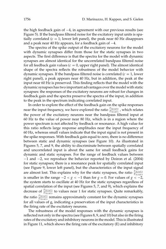
In order to explore the effect of the feedback gain on the spike responsesnear the input frequency, we have explored the ratio 52.5,67.5

72.5,87.5, which relates

the power of the excitatory neurons near the bandpass filtered input at60 Hz to the value of power near 80 Hz, which is in a region where thepower spectrum is not affected by feedback or resonance. A high value forthis ratio reflects large response amplitudes near the input frequency of60 Hz, whereas small values indicate that the input signal is not present inthe spike responses. With feedback gain equal to zero, there is no differencebetween static and dynamic synapses (see Figure 10). As illustrated inFigures 5, 7, and 9, the ability to discriminate between spatially correlatedand uncorrelated input is about the same for small feedback gains fordynamic and static synapses. For the range of feedback values between−1 and −2, we reproduce the behavior reported by Doiron et al. (2004)for static synapses; there is a resonance peak for spatially correlated input(see Figure 9, lower left panel), but the characteristics of the input signalare almost lost. This explains why for the static synapses, the ratio 52.5,67.5

72.5,87.5

is smaller in the range −2 < g < −1 than for g = 0. For values of g < −2,the system starts to oscillate at 40 Hz for the static synapses regardless ofspatial correlation of the input (see Figures 5, 7, and 9), which explains thedecrease of 52.5,67.5

72.5,87.5to values near 1 for static synapses. Quite remarkably,

the ratio 52.5,67.5 72.5,87.5

remains approximately constant for the dynamic synapsesfor all values of g, indicating a preservation of the input characteristics inthe firing rate of the excitatory neurons.

The robustness of the model responses with the dynamic synapses isreflected not only in the spectra (see Figures 8, 9, and 10) but also in the firingrates of the excitatory and inhibitory neurons in the model. This is illustratedin Figure 11, which shows the firing rate of the excitatory (E) and inhibitory


Figure 10: Discrimination index ρI F to discriminate the input frequency near60 Hz in the responses of the excitatory neurons, defined as the power around60 Hz divided by the power around 80 Hz ( 52.5,67.5

72.5,87.5) for static (open symbols, SS)

and dynamic (filled symbols, DS) synapses.

Figure 11: Firing rate of excitatory (E) and inhibitory (I) neurons for the modelswith static and dynamic synapses. Data at left (right) hand correspond to modelwith inhibitory LIF neuron with leak time constant of 6 (18) ms. Except fordifferences in time constant of inhibitory neuron, static versus dynamic synapsesand feedback gain, all other parameters were the same for all conditions.

(I) neurons for the models with static and dynamic synapses for the variousfeedback gains and for two different time constants of the inhibitory neurons(6 and 18 ms). For the static synapses, the firing rate of the excitatoryneurons decreases with increasing feedback gain. The difference in firingrate for g = 0 and g = −4 is typically about 30%. A similar decrease in firing


rate is observed for the inhibitory neurons. However, for the model withdynamic synapses, the firing rates of the excitatory and inhibitory neuronsdepend only weakly on the feedback gain. Note that this phenomenon isindependent of the time constant of the inhibitory neurons.

4 Discussion

The main results of this study can be summarized in two conclusions. Thefirst is that the different results, reported by Borgers and Kopell (2003) andby Doiron et al. (2003, 2004), who used models with the same architec-ture but with a qualitatively different behavior, can be explained by theresponses of a single model with different feedback gains. The simulationspresented here show that the same architecture with pools of excitatoryand inhibitory neurons can display a different behavior when the param-eter values are in a different range. For small and intermediate feedbackgains, the model starts to oscillate if the input to the excitatory input unitsis spatially correlated. Without correlation, the resonance peak in the spikeresponses is absent. The resonance in the model, as reported by Borgers andKopell (2003), which appears as soon as the input to the excitatory neuronsis sufficiently large (regardless of correlation between input to the neurons),is obtained if the feedback gain is sufficiently large, in agreement with theconditions for resonance in their study. Another difference between themodels by Borgers and Kopell (2003) and Doiron et al. (2003, 2004) is thatthe latter has only one inhibitory unit, whereas Borgers and Kopell havea population of inhibitory neurons. In this study we have shown that thebehavior of the model by Doiron et al. (2003, 2004) does not change if thelinear unit, which sums the spikes of the excitatory neurons and which feedsthe feedback loop, is replaced by an LIF neuron. Figure 3 shows that theresults are not affected either, when several inhibitory neurons are added inparallel. Borgers and Kopell (2005) also report that the qualitative behaviorof the model is the same if several inhibitory neurons are added. In theirstudy, suppression of excitatory cells can occur for asynchronously firinginhibitory cells. In our study, the inhibitory cells fire in synchrony for spa-tially correlated input (c = 1) and for high feedback gains. For c = 0 andfor small feedback gains, the inhibitory neurons in our model do not fire insynchrony, and neither do the excitatory cells. However, if there are severalinhibitory neurons, the network models starts oscillations at slightly higherfeedback gains than for a single inhibitory neuron. In summary, the behav-ior of the model is qualitatively the same for a single inhibitory neuron andfor the case of several inhibitory neurons.

The second conclusion of our study is that replacing synapses with a con-stant efficacy by dynamic synapses has two major implications: the modelbehavior becomes robust for changes in feedback gain and in time constantof the inhibitory LIF neuron. The resonance peak appears only for corre-lated input stimuli. Moreover, the model with dynamic synapses preserves


the characteristics of the input in the spike responses. From a biologicalperspective, this is highly relevant since it allows transmission of the tem-poral properties of the input signal while the resonance provides a labelto indicate whether the input is spatially correlated. In visual cortex cells,responses reflect the temporal properties of the stimulus in the receptivefield, but in addition can reveal gamma-frequency components (see, e.g.,Reynolds & Desimone, 1999; Roelfsema, Lamme, & Spekreijse, 2004). Inaddition, several studies (e.g., Baker, Pinches, & Lemon, 2003; Schoffelenet al., 2005) have shown that multiple EEG rhythms can occur simultane-ously, which is in contradiction with the behavior of some models in theliterature (see, e.g., Borgers & Kopell, 2003; Doiron et al., 2004), which revealoscillations only at one particular frequency.

The finding that the activity of the network can reflect both the tem-poral characteristics of the input signal (frequency of input modulations),which drives the network, and synchronous oscillations at one particularfrequency is new. Previous studies modeling neurons as coupled oscilla-tors have shown that when the width of the distribution of the intrinsicfrequencies is small compared to the coupling strength, all oscillators be-come phase-locked (Ariaratnam & Strogatz, 2001). When the distributionof intrinsic frequencies becomes larger, the network can reveal a broadspectrum of dynamics, such as frequency locking at a single frequency,incoherent firing with a broad range of frequencies, oscillator death, andhybrid solutions that combine two or more of these states, depending onthe coupling strength. Tsodyks, Mitkov, and Sompolinsky (1993) studied asystem of globally coupled oscillators with pulse interactions (mimickingcoupling by presynaptic action potentials). In such a system, the completelyphase-locked state is unstable to weak disorder. For a small inhomogeneity,the oscillators are divided in two populations, one of which exhibits phase-locked periodic behavior, whereas the other consists of unlocked oscillators,which exhibit aperiodic patterns that are only partially synchronized. In thiscontext it is important to stress, that the spectra shown in Figures 5, 6, and9 are representative for all excitatory neurons. That is, the oscillations andthe input characteristics can be found in each neuron and do not reflect apartitioning within the pool of excitatory neurons.

The novel finding that a group of neurons can code both the correlationbetween parallel neuronal input channels and the temporal characteristicsof input signals is relevant for several reasons. As explained in section 1,the phenomenon of oscillations in neuronal activity in groups of neuronshas long been known. However the functional significance is yet the subjectof speculation (see, e.g., Fries, 2005). Moreover, the neuronal mechanisms,which are responsible for the initiation of oscillatory activity, are barelyknown. It is well known that cells in visual cortex can fire in synchrony atfrequencies near 40 to 60 Hz and at the same time can reproduce the tem-poral dynamics of changes in the light in the receptive field. For example,Fries, Reynolds, Rorie, and Desimone (2001) report typical changes in firing


rate at a latency of about 25 ms in cat primary visual cortex, related to onsetand offset of a visual stimulus in the receptive field of these neurons. At thesame time, they find a correlated oscillatory activity at frequencies in therange between 40 and 70 Hz. This clearly illustrates that the activity of cellsin cat primary visual cortex reflects simultaneously temporal changes inlight falling in the receptive field as well as correlated oscillatory activity at40 to 70 Hz. Similarly, cells in visual areas V2 and V4 reflect the dynamics ofstimuli in the receptive field, but at the same time reveal correlated activityin the γ -range (Reynolds & Desimone, 1999). As far as we know, our studyis the first to show that the temporal dynamics of activity in a populationof neurons can reflect both changes in the stimulus that drives the cells andoscillatory activity.

van Vreeswijk and Hansel (2001) studied the emergence of synchronizedburst activity in networks of neurons with spike adaptation. They showedthat networks of tonically firing adapting excitatory neurons can evolveto a state where the neurons burst in a synchronized manner. These au-thors showed that synchronized bursting is robust against inhomogeneities,sparseness of the connectivity, and noise. In networks of two populations,one excitatory and one inhibitory, they found that decreasing the inhibitoryfeedback can cause the network to switch from a tonically active, asyn-chronous state to the synchronized bursting state. In our study, we haddynamic synapses instead of spike adaptation, as in the study by vanVreeswijk and Hansel (2001). Another difference is that the latter study didnot consider external input but studied tonically active neurons instead.Our study therefore is a further extension of the work of van Vreeswijkand Hansel by showing the effect of external input on the stable statesof a network with excitatory and inhibitory neurons coupled by dynamicsynapses.

In the model shown in Figure 1, the dynamic synapses were imple-mented in the feedback (i.e., the I → E) path. If the firing rate of the in-hibitory neuron increases, the efficacy of the dynamic synapses decreases,which acts like an automatic gain control. This explains partly why theresponses of the model with dynamic synapses hardly depend on the feed-back loop gain. This finding is in agreement with Pantic et al. (2003), whodemonstrated that dynamic synapses can perform good coincidence de-tection over a large range of frequencies for one suitably chosen thresholdvalue, whereas static synapses require an adaptive frequency-dependentthreshold value for good detection. In fact, the adaptation is done by thesynapses themselves. Dynamic synapses in the feedforward loop have alsobeen discussed in several studies. The common message of these studies(see, e.g., Natschlager, Maas, & Zador, 2001; Senn, Segev, & Tsodyks, 1998;Pantic et al., 2003) is that dynamic synapses in the E → I path are veryeffective in allowing a correct coincidence detection for a wide range offiring rates of the excitatory neurons without changing the base current tothe inhibitory neurons.


Initially it came as a surprise that the model shown in Figure 1 revealedoscillations also for uncorrelated noise (c = 0) for large feedback gains. Thelast term in equation 2.5 is zero for c = 0. The explanation for the unexpectedresonance is that equation 2.5 was derived using linear-response theory(see Doiron et al., 2004, and Lindner, Chacron, & Longtin, 2005, where theassumptions and mathematical analyses are explained in detail). However,the linear approximations of an LIF neuron are valid only for relatively longtime constants of the neuron, where it operates mainly as an integrator. Thisapproximation is no longer valid when the time constant of the LIF neuronis short, transforming the neuron into a coincidence detector. Similarly, ahigh-feedback gain gives rise to full inhibition of the excitatory neuronsfor each action potential of the inhibitory neuron (see Figure 4, left panel),followed by a release of excitatory output. The large inhibitory input tothe excitatory neurons synchronizes the excitatory neurons (precisely asin Borgers & Kopell, 2003), leading to a burst of activity to the inhibitoryneuron. For such volleys of synchronized input, the linear approximationfor the LIF neuron also fails.

Appendix

This appendix gives a derivation of equation 2.5. It mainly follows the linesset out in Doiron et al. (2004) and in Lindner, Chacron et al. (2005) andLindner, Doiron et al. (2005).

The input to the excitatory neurons is split into two parts. The first partconsists of the base current µ, the internal neuron-specific noise ηi (t), andthe time-independent mean of the feedback (g〈STI (t)〉 with g < 0) from theinhibitory neuron to the excitatory neuron. The second part consists of theexternal input σ�√1 − cξ j (t) + √

cξG(t)� and the time-dependent part of thefeedback from the inhibitory neurons.

Using a linear response approximation for a leaky integrate-and-fireneuron with susceptibility AE (ω) and AI (ω) (see Lindner & Schimansky-Geier, 2001; Lindner, Schimansky-Geier, & Longtin, 2002) for the excitatoryneurons and inhibitory neurons, respectively, the spectrum of the spiketrain of the excitatory neuron is given by

s Ej (ω) = s E

0, j (ω) + AE (ω)[

I j (ω) + gN

e−iωτD K Iτ (ω)s I (ω)

], (A.1)

where s Ej (ω) and s E

0, j (ω) represent the spike train of the jth excitatory neuronin the presence and absence, respectively, of the external stimulus andfeedback. K I

τ (ω) represents the postsynaptic dynamics for the synapsesfrom the inhibitory to the excitatory neurons as defined in equation 2.4 inthe frequency domain, and AE (ω) and AI (ω) represent the susceptibility inthe frequency domain with respect to the input of the excitatory neuronsand the inhibitory neurons, respectively (for details, see Doiron et al., 2004;


Lindner & Schimansky-Geier, 2001; Lindner et al., 2002). The term e−iωτD

is the Fourier representation of the time delay in the inhibitory feedbackloop. For the activity of the inhibitory neuron in the frequency domain, weobtain

s I (ω) = AI (ω)KEτ (ω)

NI∑j=1

s Ej (ω). (A.2)

Inserting equation A.2 in equation A.1 and with I j (ω) as the Fourier trans-form of I j (t) = µ + η j (t) + σ�√1 − cξ j (t) + √

cξG(t)� gives for the powerspectrum of the spike train of the jth excitatory neuron

⟨s E

j s∗E

j

⟩=

⟨s E

0, j s∗E

0, j

⟩+

⟨AE I j s∗E

0, j

⟩+ ⟨

A∗E I ∗j s E

0, j

⟩

+⟨

s E0, j A∗E g

NeiωτD K I ∗

τ AI ∗K E∗

τ

NI∑k=1

s E∗k

⟩

+⟨

s E∗0, j AE g

Ne−iωτD K I

τ AI K Eτ

NI∑k=1

s Ek

⟩+

⟨∣∣AE∣∣2 ∣∣ I j

∣∣2⟩

+⟨∣∣AE

∣∣2I j

gN

eiωτD K I ∗τ AI ∗

K E∗τ

NI∑k=1

s E∗k

⟩

+⟨∣∣AE

∣∣2I ∗

jgN

e−iωτD K Iτ AI K E

τ

NI∑k=1

s Ek

⟩

+⟨∣∣AE

∣∣2( g

N

)2 ∣∣K Iτ

∣∣2 ∣∣AI∣∣2 ∣∣K E

τ

∣∣2NE∑k,l

s Ek s E∗

l

⟩, (A.3)

where x represents the Fourier transform of x.Using that 〈s E

0, j (ω)s∗E

k (ω)〉 = 〈s E0, j (ω)I ∗

j (ω)〉 = 〈s Ej (ω)ξ ∗

k (ω)〉 =〈ξG(ω)ξ ∗

k (ω)〉 = 0 for j = k explains why the second and third termson the right-hand side of the equal sign are equal to zero.

Substitution of equation A.2 in A.1 and solving for∑NI

j=1 s Ej (ω) gives

NE∑k=1

s Ek =

NE∑j=1

s E0, j + AE

NE∑j=1

I j

1 − AE ge−iωτD K Iτ AI K E

τ

. (A.4)


Substitution of equation A.4 in A.3 and using that 〈s E0, j (ω)s∗E

k (ω)〉 =〈s E

0, j (ω)I ∗j (ω)〉 = 〈s E

j (ω)ξ ∗k(ω)〉 + 〈ξG(ω)ξ ∗

k(ω)〉 = 0 for j = k and for N → ∞so as to neglect terms of order 1/N and higher, we obtain for the powerspectrum of the spike train of the excitatory

⟨s E

j (ω)s∗E

j (ω)⟩=

⟨s E

0, j (ω)s∗E

0, j (ω)⟩+ σ 2|AE (ω)|2

+ . . . + cσ 2|AE (ω)|2 2�(AE ge−iωτD K I

τ AI K Eτ

) − ∣∣AE gK Iτ AI K E

τ

∣∣2

|1 − AE ge−iωτD K Iτ AI K E

τ |2 .

Acknowledgments

We acknowledge support from the Lorentz Center (http://www.lc.leidenuniv.nl/) for organizing a workshop, which allowed us to discussthe results of this study with Andre Longtin and Nancy Kopell. We thankMagteld Zeitler for helpful discussions.

References

Ariaratnam, J. T., & Strogatz, S. H. (2001). Phase diagram for the Winfree model ofcoupled nonlinear oscillators. Phys. Rev. Lett., 86, 4278–4281.

Baker, S. N., Pinches, E. M., & Lemon, R. N. (2003). Synchronization in monkey motorcortex during a precision grip task. II: Effect of oscillatory activity on corticospinaloutput. J. Neurophysiol., 89, 1941–1953.

Borgers, C., & Kopell, N. (2003). Synchronization in networks of excitatory andinhibitory neurons with sparse, random connectivity. Neural Comp., 15, 509–538.

Buzsaki, G., Leung, L. W. S., & Vanderwolf, C. H. (1983). Cellular bases of hippocam-pal EEG in the behaving rat. Brain Res. Rev., 6, 139–171.

Doiron, B., Chacron, M. J., Maler, L., Longtin, A., & Bastian J. (2003). Inhibitoryfeedback required for network oscillatory responses to communication but notprey stimuli. Nature, 421, 539–543.

Doiron, B., Lindner, B., Longtin, A., Maler, L., & Bastian, J. (2004). Oscillatory activityin electrosensory neurons increases with the spatial correlation of the stochasticinput stimulus. Phys. Rev. Lett., 93, 048101–048104.

Ermentrout, G. B., & Kopell, N. (1986). Parabolic bursting in an excitable systemcoupled with a slow oscillation. SIAM J. Appl. Math., 46, 233–253.

Ernst, U., Pawelzik, K., & Geisel, T. (1995). Synchronization induced by temporaldelays in pulse-coupled oscillators. Phys. Rev. Lett., 74, 1570–1573.

Fries, P. (2005). A mechanism for cognitive dynamics: Neuronal communicationthrough neuronal coherence. Trends in Cognitive Sciences, 9, 474–480.

Fries, P., Reynolds, J. H., Rorie, A. E., & Desimone, R. (2001). Modulation of oscillatoryneuronal synchronization by selective visual attention. Science, 291, 1560–1563.

Gray, C. M. (1994). Synchronous oscillations in neuronal systems: Mechanisms andfunctions. J. Comp. Neurosci., 1, 11–38.


Gutkin, B. S., & Ermentrout, G. B. (1998). Dynamics of membrane excitability deter-mine interspike interval variability: A link between spike generation mechanismsand cortical spike train statistics. Neural Comp., 10, 1047–1065.

Hansel, D., & Mato, G. (1993). Patterns of synchrony in a heterogeneous Hodgkin-Huxley neural-network with weak-coupling. Physica A, 200, 662–669.

Hansel, D., Mato, G., & Meunier, C. (1995). Synchrony in excitatory neural networks.Neural Comp., 7, 307–337.

Hoppensteadt, F. C., & Izhikevich, E. M. (1997). Weakly connected neural networks.New York: Springer-Verlag.

Lindner, B., Chacron, M. J., & Longtin, A. (2005). Integrate-and-fire neurons withthreshold noise: A tractable model of how interspike interval correlations affectneuronal signal transmission. Phys. Rev., E, 72, 021911.

Lindner, B., Doiron, B., & Longtin, A. (2005). Theory of oscillatory firing inducedby spatially correlated noise and delayed inhibitory feedback. Phys. Rev. E, 72,061919.

Lindner, B., & Schimansky-Geier, L. (2001). Transmission of noise coded versusadditive signals through a neuronal ensemble. Phys. Rev. Lett., 86, 2934–2937.

Lindner, B., Schimansky-Geier, L., & Longtin, A. (2002). Maximizing spike traincoherence or incoherence in the leaky integrate-and-fire model. Phys. Rev. E, 66,031916.

Lytton, W. W., & Sejnowski, T. J. (1991). Simulations of cortical pyramidal neuronssynchronized by inhibitory interneurons. J. Neurophysiol., 66, 1059–1079.

Mirollo, R. E., & Strogatz, S. H. (1990). Synchronization of pulse-coupled biologicaloscillators. SIAM J. Appl. Math., 50, 1645–1662.

Natschlager, T., Maass, W., & Zador, A. (2001). Efficient temporal processing withbiologically realistic dynamic synapses. Network Computation in Neural Systems,12, 75–87.

Pantic, L., Torres, J. J., & Kappen, H. J. (2003). Coincidence detection with dynamicsynapses. Network Computation in Neural Systems, 14(1), 17–33.

Reynolds, J. H., Chelazzi, L., & Desimone, R. (1999). Competitive mechanisms sub-serve attention in macaque areas V2 and V4. J. Neurosci., 19, 1736–1753.

Reynolds, J. H., & Desimone, R. (1999). The role of neural mechanisms of attentionin solving the binding problem. Neuron, 24, 19–29.

Roelfsema, P., Lamme, V. A. F., & Spekreijse, H. (2004). Synchrony and covariation offiring rates in the primary visual cortex during contour grouping. Nature Neurosci,7, 982–991.

Rudolph, M., & Destexhe, A. (2003). Tuning neocortical pyramidal neurons betweenintegrators and coincidence detectors. J. Comp. Neurosci., 14, 239–251.

Schoffelen, J. M., Oostenveld, R., & Fries, P. (2005). Neuronal coherence as a mecha-nism of effective corticospinal interaction. Science, 308, 111–113.

Senn, W., Segev, I., & Tsodyks, M. (1998). Reading neuronal synchrony with depress-ing synapses. Neural Comp., 10, 815–819.

Singer, W. (1999). Neuronal synchrony: A versatile code for the definition of rela-tions? Neuron, 24(1), 49–65.

Singer, W., & Gray, C. M. (1995). Visual feature integration and the temporal corre-lation hypothesis. Annu. Rev. Neurosci., 18, 555–586.


Traub, R. D., Whittington, M. A., Colling, S. B., Buzsaki, G., & Jefferys, J. G. R. (1996).Analysis of gamma rhythms in the rat hippocampus in vitro and in vivo. J. Physiol.(London), 493, 471–484.

Tsodyks, M. V., & Markram, H. (1997). The neural code between neocortical pyrami-dal neurons depends on neurotransmitter release probability. Proc. Natl. Ac. Sci.USA, 94, 719–723.

Tsodyks, M., Mitkov, I., & Sompolinsky, H. (1993). Pattern of synchrony in inho-mogeneous networks of oscillators with pulse interactions. Phys. Rev. Lett., 71,1280–1283.

Tsodyks, M., Pawelzik, K., & Markram, H. (1998). Neural networks with dynamicsynapses. Neural Comp., 10, 821–835.

Tsodyks, M., Uziel, A., & Markram, H. (2000). Synchrony generation in recurrentnetworks with frequency-dependent synapses. J. Neurosci., 20(RC50), 1–5.

van Vreeswijk, C. (2000). Analysis of the asynchronous state in networks of stronglycoupled oscillators. Phys. Rev. Lett., 84, 5110–5113.

van Vreeswijk, C., & Hansel, D. (2001). Patterns of synchrony in neural networkswith spike adaptation. Neural Comp., 13, 959–992.

Whittington, M. A., Traub, R. D., & Jeffreys, J. G. R. (1995). Synchronized oscillationsin interneuron networks driven by metabotropic glutamate receptor activation.Nature, 373, 612–615.

Received January 30, 2006; accepted November 8, 2006.

Input-Driven Oscillations in Networks with Excitatory and

Documents

Transcript of Input-Driven Oscillations in Networks with Excitatory and