Innovization: Innovative Design Principles Through

Optimization

Kalyanmoy Deb and Aravind SrinivasanKanpur Genetic Algorithms Laboratory (KanGAL)

Indian Institute of Technology KanpurKanpur, PIN 208016, India

Email: {deb,aravinds}@iitk.ac.inhttp://www.iitk.ac.in/kangal/pub.htm

KanGAL Report Number 2005007

Abstract

This paper introduces a new design methodology (we called it an “innovization” task) in thecontext of finding new and innovative design principles by means of optimization techniques.Although optimization algorithms are routinely used to find an optimal solution correspondingto an optimization problem, the task of innovization stretches the scope beyond an optimiza-tion task and attempts to unveil new and innovative design principles relating to decisionvariables and objectives, so that a deeper understanding of the problem can be obtained.After describing the innovization procedure and its difference from a standard optimizationprocedure, the innovization procedure is applied to a number of engineering design problems.The variety of problems chosen in the paper and the resulting innovations obtained for eachproblem amply demonstrate the usefulness of the innovization task. The results should encour-age a wide spread applicability of the proposed innovization procedure (which is not simplyan optimization procedure) to other problem-solving tasks.

Keywords: Innovative design, optimization, engineering design, evolutionary optimization, multi-objective optimization, commonality principles, Pareto-optimal solutions.

1 Introduction

Innovation, defined in Oxford American Dictionary as ‘the act of introducing a new process orthe way of doing new things’ has always fascinated man. In the context of engineering design ofa system, a product or a process, researchers and applicationists constantly look for innovativesolutions. Unfortunately, there exist very few scientific and systematic procedures for achievingsuch innovations. Goldberg [12] narrates that a competent genetic algorithm – a search andoptimization procedure based on natural evolution and natural genetics – can be an effectivemean to arrive at an innovative design for a single objective scenario.

In this paper, we extend Goldberg’s argument and describe a systematic procedure involvinga multi-objective optimization task and a subsequent analysis of optimal solutions to arrive ata deeper understanding of the problem, and not simply to find a single optimal (or innovative)solution. In the process of understanding insights about the problem, the systematic proceduresuggested here may often decipher new and innovative design principles which are common tooptimal trade-off solutions and were not known earlier. Such commonality principles amongmultiple solutions should provide a reliable procedure of arriving at a ‘blue-print’ or a ‘recipe’ forsolving the problem in an optimal manner. Through a number of engineering design problems,

1

we describe the proposed ‘innovization’ process and present resulting innovized design principleswhich are useful, not obvious from the appearance of the problem, and also not possible to achieveby a single-objective optimization task.

In the remainder of the paper, we describe the importance of considering multiple conflictingobjectives in an innovative design task in Section 2. Thereafter, we present the proposed in-novization procedure in Section 3. The innovization task is illustrated by applying the procedureon a number of engineering design problems in Sections 4 to 8. Finally, conclusions are made inSection 9.

2 Multiple Conflicting Objectives of Design

The main crux of the proposed innovization procedure involves optimization of at least twoconflicting objectives of a design. When a design is to be achieved for a single goal of minimizingsize of a product or of maximizing output from the product, usually one optimal solution is thetarget. When optimized, the optimal solution portrays the design, fixes the dimensions, andimplies not much more. Although a sensitivity analysis can provide some information about therelative importance of constraints, they only provide local information close to the single optimumsolution. Truly speaking, such an optimization task of finding a single optimum design does notoften give a designer any deeper understanding than what and how the optimum solution shouldlook like. After all, how much a single (albeit optimal) solution in the entire search space ofsolutions can offer to anyone?

Let us now think of an optimum design procedure in the context of two or more conflictinggoals. Say, we are interested in the design of a product for minimum size and for maximum outputsimultaneously. Ideally, such a bi-objective optimization task results in a set of optimal solutions,known as Pareto-optimal solutions, each portraying a trade-off between the two objectives [19,6]. Out of these optimal solutions lies a solution (say solution A) which is the best for sizeconsideration and a hopefully a different solution (say solution B) which is the best for outputconsideration. There also lie a host of many other solutions which are not as good as A in termsof size or not as good as B in terms of delivered output, but these intermediate solutions aregood compromises to solutions A and B. There exist a plethora of classical and evolutionaryapproaches to arrive at a number of such Pareto-optimal solutions iteratively and reliably [6, 3,2, 19]. However, we are not simply interested in finding a set of such optimal trade-off solutions,rather find them and analyze them for discovering some interesting commonality principles inthem.

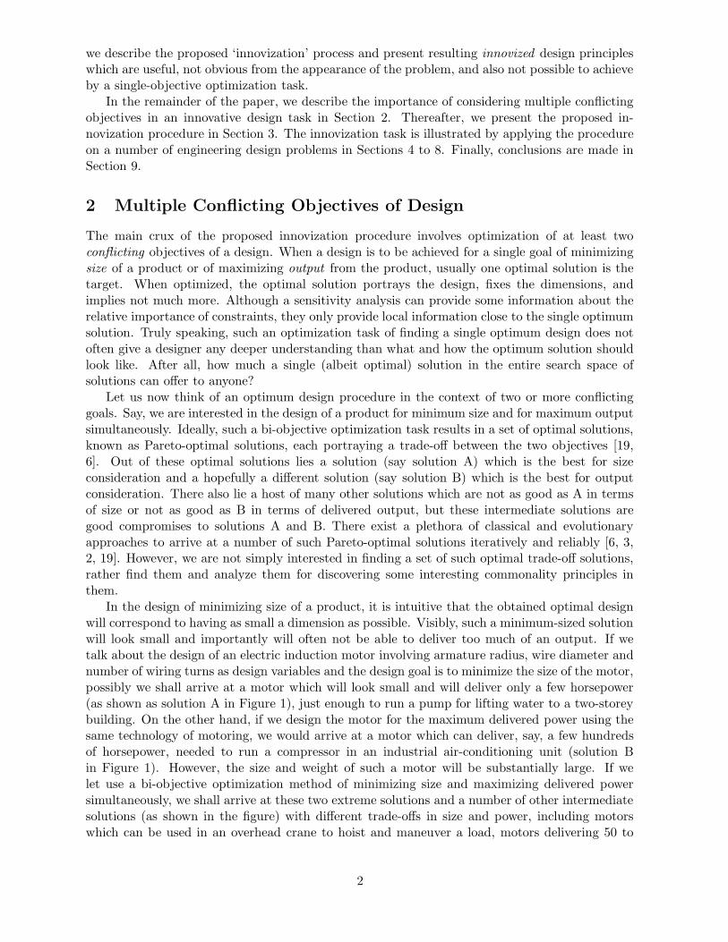
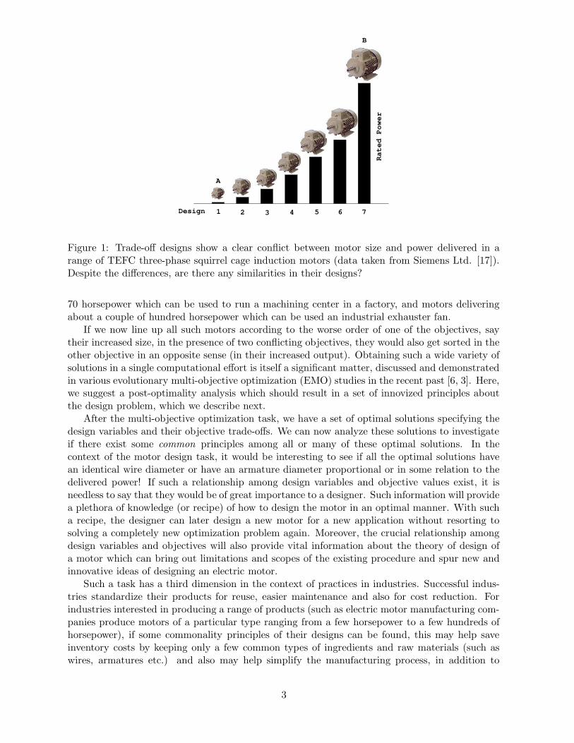
In the design of minimizing size of a product, it is intuitive that the obtained optimal designwill correspond to having as small a dimension as possible. Visibly, such a minimum-sized solutionwill look small and importantly will often not be able to deliver too much of an output. If wetalk about the design of an electric induction motor involving armature radius, wire diameter andnumber of wiring turns as design variables and the design goal is to minimize the size of the motor,possibly we shall arrive at a motor which will look small and will deliver only a few horsepower(as shown as solution A in Figure 1), just enough to run a pump for lifting water to a two-storeybuilding. On the other hand, if we design the motor for the maximum delivered power using thesame technology of motoring, we would arrive at a motor which can deliver, say, a few hundredsof horsepower, needed to run a compressor in an industrial air-conditioning unit (solution Bin Figure 1). However, the size and weight of such a motor will be substantially large. If welet use a bi-objective optimization method of minimizing size and maximizing delivered powersimultaneously, we shall arrive at these two extreme solutions and a number of other intermediatesolutions (as shown in the figure) with different trade-offs in size and power, including motorswhich can be used in an overhead crane to hoist and maneuver a load, motors delivering 50 to

2

1 2 3 4 5 6 7

Rated Power

B

Design

A

Figure 1: Trade-off designs show a clear conflict between motor size and power delivered in arange of TEFC three-phase squirrel cage induction motors (data taken from Siemens Ltd. [17]).Despite the differences, are there any similarities in their designs?

70 horsepower which can be used to run a machining center in a factory, and motors deliveringabout a couple of hundred horsepower which can be used an industrial exhauster fan.

If we now line up all such motors according to the worse order of one of the objectives, saytheir increased size, in the presence of two conflicting objectives, they would also get sorted in theother objective in an opposite sense (in their increased output). Obtaining such a wide variety ofsolutions in a single computational effort is itself a significant matter, discussed and demonstratedin various evolutionary multi-objective optimization (EMO) studies in the recent past [6, 3]. Here,we suggest a post-optimality analysis which should result in a set of innovized principles aboutthe design problem, which we describe next.

After the multi-objective optimization task, we have a set of optimal solutions specifying thedesign variables and their objective trade-offs. We can now analyze these solutions to investigateif there exist some common principles among all or many of these optimal solutions. In thecontext of the motor design task, it would be interesting to see if all the optimal solutions havean identical wire diameter or have an armature diameter proportional or in some relation to thedelivered power! If such a relationship among design variables and objective values exist, it isneedless to say that they would be of great importance to a designer. Such information will providea plethora of knowledge (or recipe) of how to design the motor in an optimal manner. With sucha recipe, the designer can later design a new motor for a new application without resorting tosolving a completely new optimization problem again. Moreover, the crucial relationship amongdesign variables and objectives will also provide vital information about the theory of design ofa motor which can bring out limitations and scopes of the existing procedure and spur new andinnovative ideas of designing an electric motor.

Such a task has a third dimension in the context of practices in industries. Successful indus-tries standardize their products for reuse, easier maintenance and also for cost reduction. Forindustries interested in producing a range of products (such as electric motor manufacturing com-panies produce motors of a particular type ranging from a few horsepower to a few hundreds ofhorsepower), if some commonality principles of their designs can be found, this may help saveinventory costs by keeping only a few common types of ingredients and raw materials (such aswires, armatures etc.) and also may help simplify the manufacturing process, in addition to

3

cutting down the need for specialized man-powers.It is argued elsewhere [7] that since the Pareto-optimal solutions are not any arbitrary so-

lutions, rather solutions which mathematically must satisfy the so-called Fritz-John necessaryconditions (involving gradients of objective and constraint functions) [13], in engineering and sci-entific systems and problems, we may be reasonably confident in claiming that there would existsome commonalities (or similarities) among the Pareto-optimal solutions which will ensure theiroptimality. On the other hand, there would exist some dissimilarities among them which willmake them different from each other and place them on various locations on the Pareto-optimalfrontier providing an optimal trade-off among objectives. Whether such similarities exist for allsolutions on the Pareto-optimal front or some kind of similarity exist partially among solutions ona part of the Pareto-optimal front and another kind of similarity exists in another part of the frontor there exist hierarchical (or level-wise) similarities (some kind to all and some sub-kind to a por-tion of the front) are matters which may vary from problem to problem. Whatever is the extent ofcommonalities, if exist, must portray some design principles which are worth knowing. We argueand demonstrate amply in the subsequent sections that such design principles deciphered fromthe obtained Pareto-optimal solutions may often bring out new and innovative principles whichwere unknown earlier. They are also useful in design activities and provide a better understandingof parameter interactions. Since these innovative principles are derived through the outcome of acarefully performed optimization task, we call this procedure an act of ‘innovization’ – a processof obtaining innovative solutions and design principles through optimization.

3 Innovization Procedure

As described above, the analysis of the optimized solutions will result in worthwhile design prin-ciples, if the trade-off solutions are really close to the optimal solutions or if they are exactlyon the Pareto-optimal frontier. Since for engineering and complex scientific problem-solving, weneed to use a numerical optimization procedure and since in such problems, the exact optimum isnot known a priori, adequate experimentation and verification must have to be done first to gainconfidence about the closeness of the obtained solutions to the actual Pareto-optimal front. In allcase studies performed here, we have used the well-known elitist non-dominated sorting geneticalgorithm or NSGA-II [8] as the multi-objective optimization tool. NSGA-II begins its searchwith a random population of solutions and iteratively progresses towards the Pareto-optimalfront so that at the end of a simulation run, multiple trade-off optimal solutions are obtainedsimultaneously. Due to its simplicity and efficacy, NSGA-II is adopted in a number of commercialoptmization softwares and has been extensively applied to various multi-objective optimizationproblems in the past few years. For a detail procedure of NSGA-II, readers are referred to theoriginal study [8]. The NSGA-II solutions are then clustered to identify a few well-distributedsolutions. The clustered NSGA-II solutions are then modified by using a local search procedure(we have used Benson’s method [1, 6] here). The obtained NSGA-II-cum-local-search solutionsare then verified by two independent procedures:

1. The extreme Pareto-optimal solutions are verified by running a single-objective optimiza-tion procedure (a genetic algorithm is used here) independently on each objective functionsubjected to satisfying given constraints.

2. Some intermediate Pareto-optimal solutions are verified by using the normal constraintmethod (NCM) [18] starting at different locations on the hyper-plane constructed using theindividual best solutions obtained from the previous step.

When the attainment of optimized solutions and their verifications are made, ideally a data-mining strategy must be used to automatically evolve design principles from the combined data of

4

optimized design variables and corresponding objective values. By no means this is an easy taskand is far from being a simple regression task of fitting a model over a set of multi-dimensionaldata. We mentioned some such difficulties earlier: (i) there may exist multiple relationships whichare all needed to be found by the automated programming, thereby requiring to find multiplesolutions to the problem simultaneously, (ii) a relationship may exist partially to the data set,thereby requiring a clustering procedure to identify which design principles are valid on whichclusters, and (iii) since optimized data may not exactly be the optimum data, exact relationshipsmay not be possible to achieve, thereby requiring to use fuzzy rule or rough set based approaches.While we are currently pursuing various data-mining and machine learning techniques for anautomated learning and deciphering of such important design principles from optimized data set,in this paper we mainly use visual and statistical comparisons and graph plotting softwares forthe task.

We present the proposed innovization procedure here:

Step 1: Find individual optimum solution for each of the objectives by using a single-objectiveGA (or sometimes using NSGA-II by specifying only one objective) or by a classical method.Thereafter, note down the ideal point.

Step 2: Find the optimized multi-objective front by NSGA-II. Also, obtain and note the nadirpoint1 from the front.

Step 3: Normalize all objectives using ideal and nadir points and cluster a few solutions Z (k)

(k = 1, 2, . . . , 10), preferably in the area of interest to the designer or uniformly along theobtained front.

Step 4: Apply a local search (Benson’s method [1] is used here) and obtain the modified opti-mized front.

Step 5: Perform the normal constraint method (NCM) [18] starting at a few locations to verifythe obtained optimized front. These solutions constitute a reasonably confident optimizedfront.

Step 6: Analyze the solutions for any commonality principles as plausible innovized relationships.

Since the above innovization procedure is expected to be applied to a problem once and for all,designers may not be quite interested in the computational time needed to complete the task.However, if needed, the above procedure can be made faster by parallelizing Steps 1, 2, 4 and 5on a distributed computing machine.

We now illustrate the working of the above innovization procedure on a number of engineeringapplications. In all problems solved in this paper, we use sufficiently large population size andrun an evolutionary multi-objective optimization algorithm (NSGA-II) for sufficient generationsso as to have confidence on the obtained trade-off frontier.

4 Two-Member Truss Design

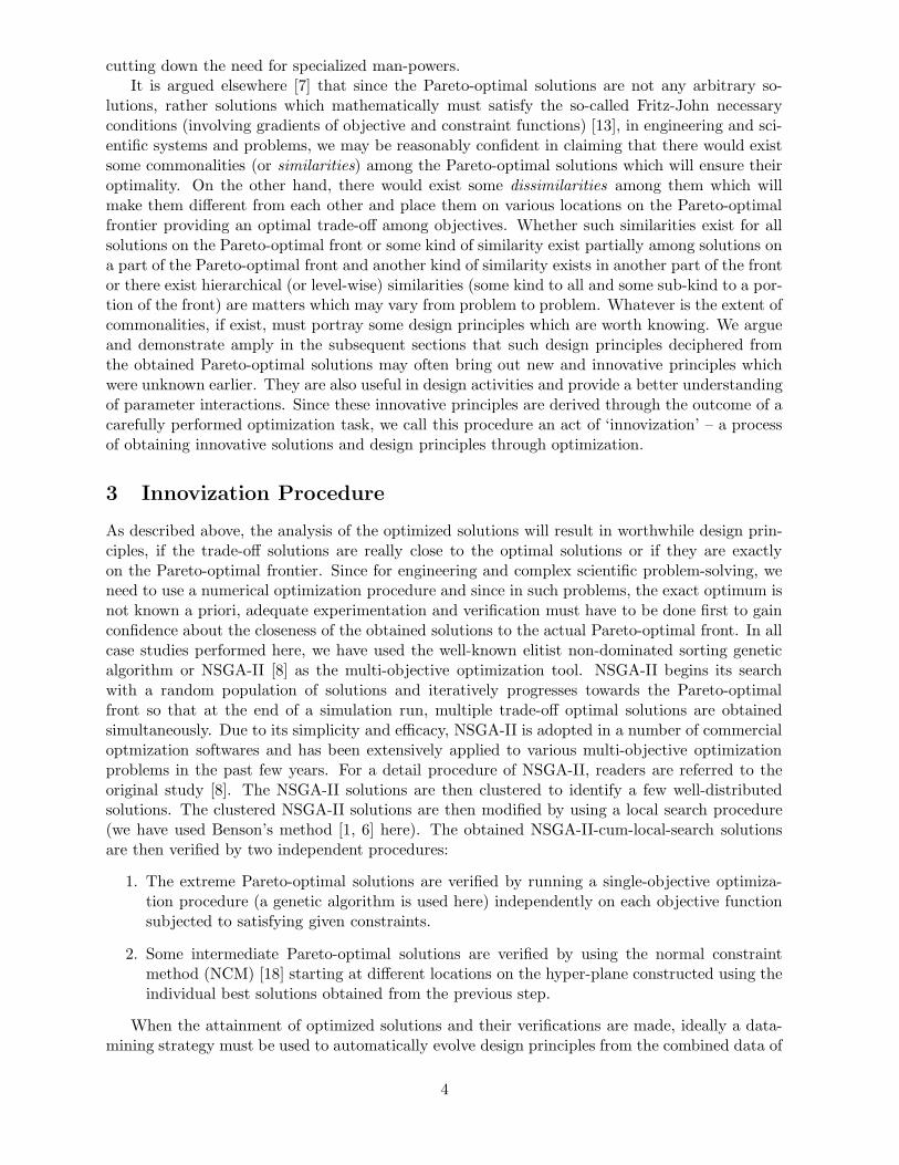
We begin with a three-variable, two-objective truss design problem. This problem was originallystudied using the ε-constraint method [2, 19] and later by an evolutionary approach [6], but wasnever attempted to verify the optimality of the obtained solutions. The truss (Figure 2) has tocarry a certain load without elastic failure. We consider two objectives of design: (i) minimize

1It is interesting to note that finding a set of trade-off Pareto-optimal solutions using an evolutionary multi-objective optimization (EMO) procedure is one way of arriving at the nadir point. Finding the nadir point is animportant task in the classical multi-criterion decision-making approaches and is also reported to be a difficult task[15].

5

����������

x1

������

100 kN

1m4m

yx2

AB

C

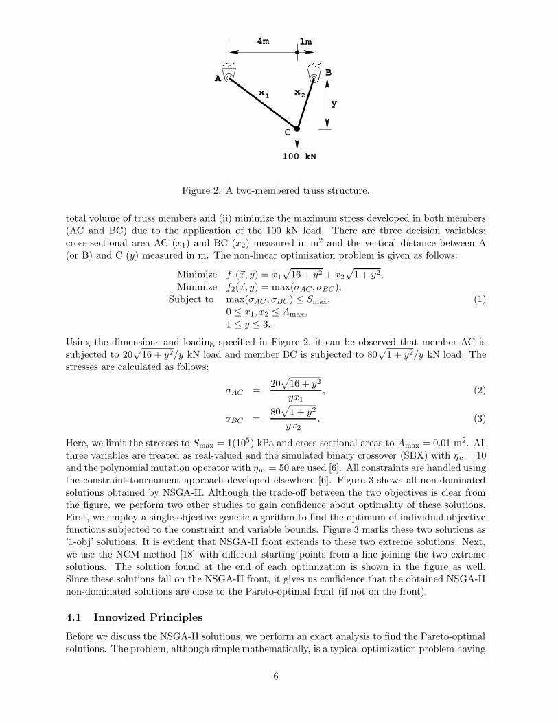
Figure 2: A two-membered truss structure.

total volume of truss members and (ii) minimize the maximum stress developed in both members(AC and BC) due to the application of the 100 kN load. There are three decision variables:cross-sectional area AC (x1) and BC (x2) measured in m2 and the vertical distance between A(or B) and C (y) measured in m. The non-linear optimization problem is given as follows:

Minimize f1(~x, y) = x1

√

16 + y2 + x2

√

1 + y2,Minimize f2(~x, y) = max(σAC , σBC),

Subject to max(σAC , σBC) ≤ Smax,0 ≤ x1, x2 ≤ Amax,1 ≤ y ≤ 3.

(1)

Using the dimensions and loading specified in Figure 2, it can be observed that member AC issubjected to 20

√

16 + y2/y kN load and member BC is subjected to 80√

1 + y2/y kN load. Thestresses are calculated as follows:

σAC =20

√

16 + y2

yx1, (2)

σBC =80

√

1 + y2

yx2. (3)

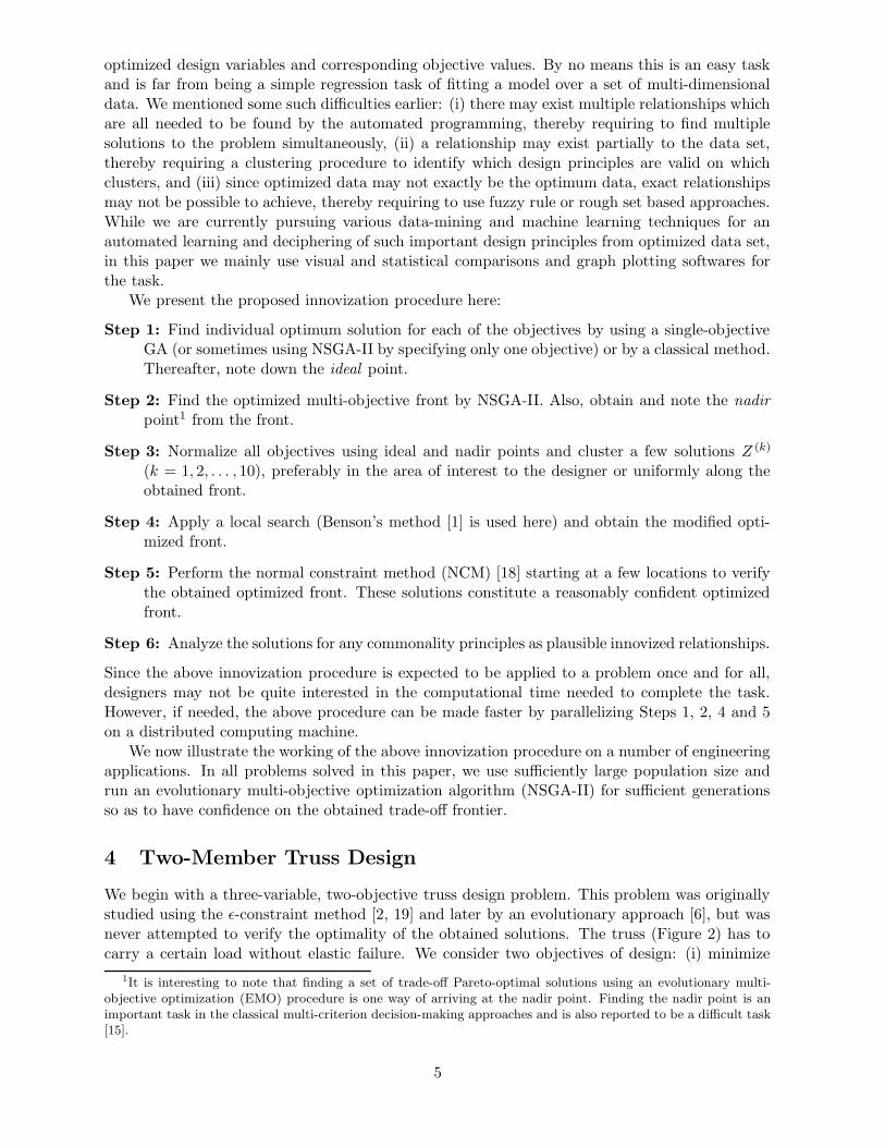
Here, we limit the stresses to Smax = 1(105) kPa and cross-sectional areas to Amax = 0.01 m2. Allthree variables are treated as real-valued and the simulated binary crossover (SBX) with ηc = 10and the polynomial mutation operator with ηm = 50 are used [6]. All constraints are handled usingthe constraint-tournament approach developed elsewhere [6]. Figure 3 shows all non-dominatedsolutions obtained by NSGA-II. Although the trade-off between the two objectives is clear fromthe figure, we perform two other studies to gain confidence about optimality of these solutions.First, we employ a single-objective genetic algorithm to find the optimum of individual objectivefunctions subjected to the constraint and variable bounds. Figure 3 marks these two solutions as’1-obj’ solutions. It is evident that NSGA-II front extends to these two extreme solutions. Next,we use the NCM method [18] with different starting points from a line joining the two extremesolutions. The solution found at the end of each optimization is shown in the figure as well.Since these solutions fall on the NSGA-II front, it gives us confidence that the obtained NSGA-IInon-dominated solutions are close to the Pareto-optimal front (if not on the front).

4.1 Innovized Principles

Before we discuss the NSGA-II solutions, we perform an exact analysis to find the Pareto-optimalsolutions. The problem, although simple mathematically, is a typical optimization problem having

6

two resource terms in objectives involving variables x1 and x2 each and interlinking them withanother variable y. For such problems, the optimum occurs when the identical resource allocationbetween two terms in both objective and constraint functions are made:

x1

√

16 + y2 = x2

√

1 + y2, (4)

20√

16 + y2

yx1=

80√

1 + y2

yx2. (5)

Thus, every optimum solution is expected to satisfy both the above equations, yielding y = 2 andx1/x2 = 0.5. Using y = 2 m in the expression for the first (volume) objective, we can also obtainx2 = V/2

√5 m2, where V is the volume (in m3) of the structure. Substituting these values to

the objective functions V = f1 and S = f2, we also obtain SV = 400 kN – an inverse relationshipbetween the objectives. Thus, the solutions in the Pareto-optimal front are given in terms ofvolume V , as follows:

x1 =V

4√

5m2, x2 =

V

2√

5m2, y = 2 m, S = 400/V kPa.

When the variable x2 reaches its maximum limit, that is, at the transition point, V = 0.04472 m3

and S = 8, 944.26 kPa, and x2 cannot be increased any further. Interestingly, volume V can stillbe increased in an optimal manner, as we shall see later.

The inset plot (drawn with a logarithmic scale of both axes) in Figure 3 shows this interestingaspect of the obtained front. There are two distinct behaviors of the optimal front around thetransition point T marked in the figure: (i) one spanning from the smallest-volume solution toabout a volume of about 0.04478 m3 (point T), and (ii) another spanning from this transition pointtill the smallest-stress solution. The extreme solutions and this intermediate solution, obtained

SV=Constant

T

T

Volume (m^3)

Maximum Stress (kPa)

100000

70000

50000

20000

10000

70000.10.070.045.020.010.0050.002

Maximum Stress (kPa)

Volume (m^3)

NCM1−obj

NSGA−II

0.05 0.04 0.03 0.02 0.01 0 0

20000

40000

60000

80000

100000

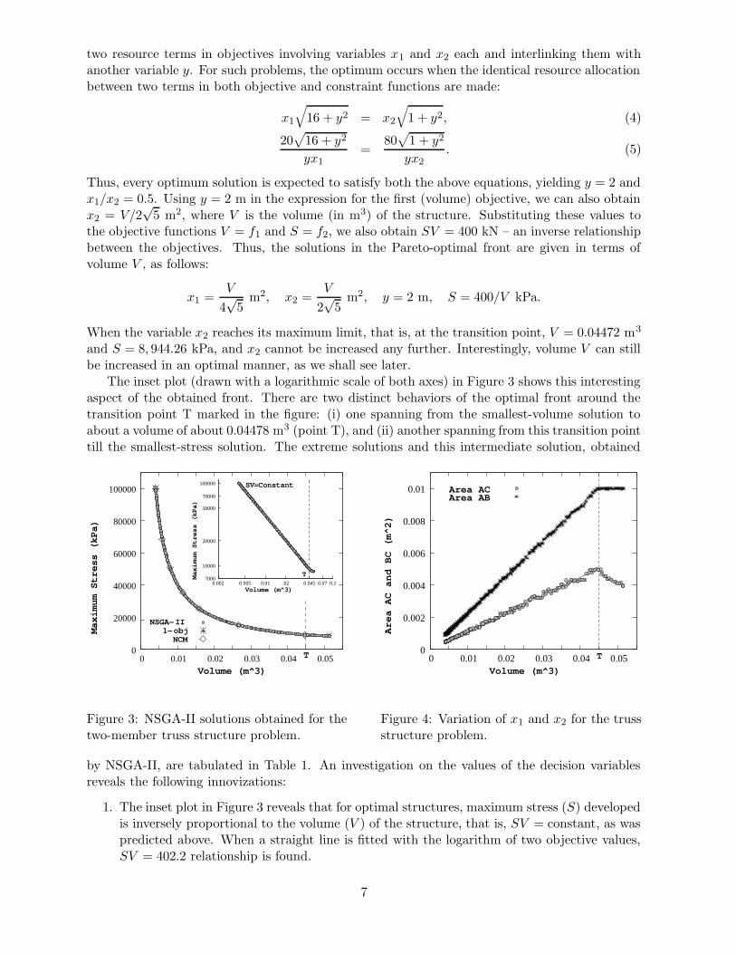
Figure 3: NSGA-II solutions obtained for thetwo-member truss structure problem.

T 0

0.002

0.004

0.006

0.008

0.01

0 0.01 0.04 0.05Volume (m^3)

Area AC and BC (m^2)

Area ACArea AB

0.02 0.03

Figure 4: Variation of x1 and x2 for the trussstructure problem.

by NSGA-II, are tabulated in Table 1. An investigation on the values of the decision variablesreveals the following innovizations:

1. The inset plot in Figure 3 reveals that for optimal structures, maximum stress (S) developedis inversely proportional to the volume (V ) of the structure, that is, SV = constant, as waspredicted above. When a straight line is fitted with the logarithm of two objective values,SV = 402.2 relationship is found.

7

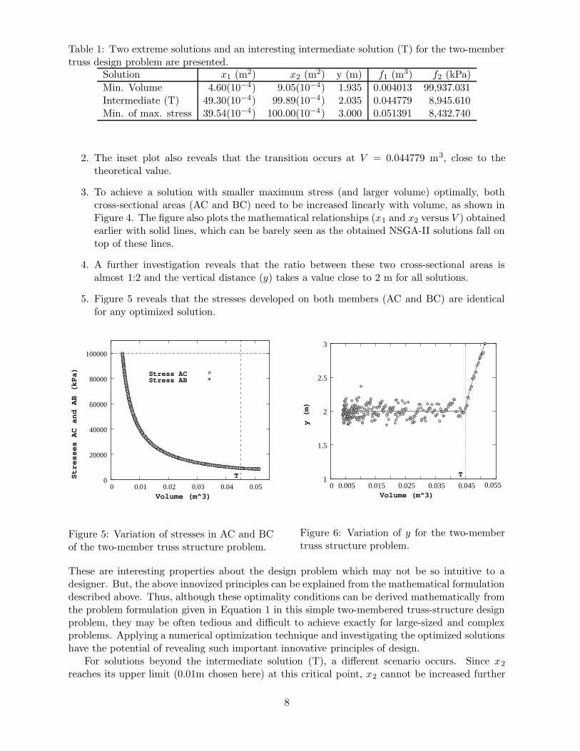
Table 1: Two extreme solutions and an interesting intermediate solution (T) for the two-membertruss design problem are presented.

Solution x1 (m2) x2 (m2) y (m) f1 (m3) f2 (kPa)

Min. Volume 4.60(10−4) 9.05(10−4) 1.935 0.004013 99,937.031Intermediate (T) 49.30(10−4) 99.89(10−4) 2.035 0.044779 8,945.610Min. of max. stress 39.54(10−4) 100.00(10−4) 3.000 0.051391 8,432.740

2. The inset plot also reveals that the transition occurs at V = 0.044779 m3, close to thetheoretical value.

3. To achieve a solution with smaller maximum stress (and larger volume) optimally, bothcross-sectional areas (AC and BC) need to be increased linearly with volume, as shown inFigure 4. The figure also plots the mathematical relationships (x1 and x2 versus V ) obtainedearlier with solid lines, which can be barely seen as the obtained NSGA-II solutions fall ontop of these lines.

4. A further investigation reveals that the ratio between these two cross-sectional areas isalmost 1:2 and the vertical distance (y) takes a value close to 2 m for all solutions.

5. Figure 5 reveals that the stresses developed on both members (AC and BC) are identicalfor any optimized solution.

T

Stress ACStress AB

Volume (m^3)

Stresses AC and AB (kPa)

0 0.01 0.02 0.03 0.04 0.05 0

20000

40000

60000

80000

100000

Figure 5: Variation of stresses in AC and BCof the two-member truss structure problem.

T 1

1.5

2

2.5

3

0 0.005 0.015 0.025 0.035 0.045 0.055Volume (m^3)

y (m)

Figure 6: Variation of y for the two-membertruss structure problem.

These are interesting properties about the design problem which may not be so intuitive to adesigner. But, the above innovized principles can be explained from the mathematical formulationdescribed above. Thus, although these optimality conditions can be derived mathematically fromthe problem formulation given in Equation 1 in this simple two-membered truss-structure designproblem, they may be often tedious and difficult to achieve exactly for large-sized and complexproblems. Applying a numerical optimization technique and investigating the optimized solutionshave the potential of revealing such important innovative principles of design.

For solutions beyond the intermediate solution (T), a different scenario occurs. Since x2

reaches its upper limit (0.01m chosen here) at this critical point, x2 cannot be increased further

8

and it remains fixed to this upper limit for all larger volume solutions. However, two optimalityproperties – (i) the stresses in both members continue to have identical values and (ii) relationshipbetween two cross-sectional sizes dictated by Equation 4 continues to hold good. But, now x1

and y gets adjusted in a different manner: y (in m) is increased and x1 (in m2) is reduced withan increase in overall volume (V in m3) of the structure, as given below:

y =

√

3200V 2 + 40V√

6400V 2 − 12 − 4, (6)

x1 = 0.0025

√

16 + y2

1 + y2. (7)

Beyond this critical point (T), since x2 cannot be increased any further, the only way to reducethe stresses is to increase y in a manner so as to make the stresses in both members equal. Anincrease of y increases the length of the members, but decreases the component of the applied loadon each member. Thus, a smaller cross-sectional area can be used to withstand the smaller loadcausing a smaller developed stress. Equation 7 shows how the cross-section must be decreased asa function of y.

Following observations can be made from the obtained solutions:

1. All NSGA-II solutions having a volume larger than the transition solution (T) is found tohave a fixed x2 = 0.01 m2 (upper limit of x2).

2. Figure 4 also verifies that beyond the transition point T, x1 decreases with volume.

3. To verify the variation of y with V given in Equation 6, Figure 6 is plotted with NSGA-IIsolutions and with Equation 6. The optimal relationship between the two objectives is asfollows: SV = (4 + y2)/(0.01y). Since for Pareto-optimal solutions having V > 0.04472 m3,the parameter y increases with V , the quantity SV increases with V , as depicted in theinset plot of Figure 3.

Some of the above properties (such as, the existence and location of the transition point, cross-sectional area x2 being constant beyond the transition point, and reduction of x1 beyond the tran-sition point to increase V optimally) are difficult to comprehend from the problem formulation andimportantly are also difficult to obtain by any other means, including multiple single-objective op-timizations of different weighted-sum problems. Even though, a classical weighted-sum approachcan be used to get a few points on the Pareto-optimal front, finding the transition point accidentlywith a particular weight vector will be highly unlikely.

4.2 Higher-Level Innovizations

Before we leave this case study, we would like to raise another important aspect of the innovizationprocedure. Since an analysis is performed on the solutions obtained by solving a particularoptimization problem (that is, for fixed values of all problem parameters), one may wonder how theinnovized results will change if different parameter values were used. In the context of the abovetruss-structure design, the parameters kept fixed for the entire analysis were: (i) upper limit ofdeveloped stress, Smax, (ii) upper limit of cross-sectional areas, Amax, (iii) lower and upper boundof y. It would be interesting to investigate whether the innovized principles deciphered above willstill be valid parametrically for variations of these parameters! For example, one may think thatthe reason for the fixed-x2 solutions (near smallest stress value) occurred due to the use of a smallAmax. It may be worthwhile to ponder whether the two-pronged behavior of the Pareto-optimalfront observed above would still remain, if the cross-sectional limit Amax is increased.

9

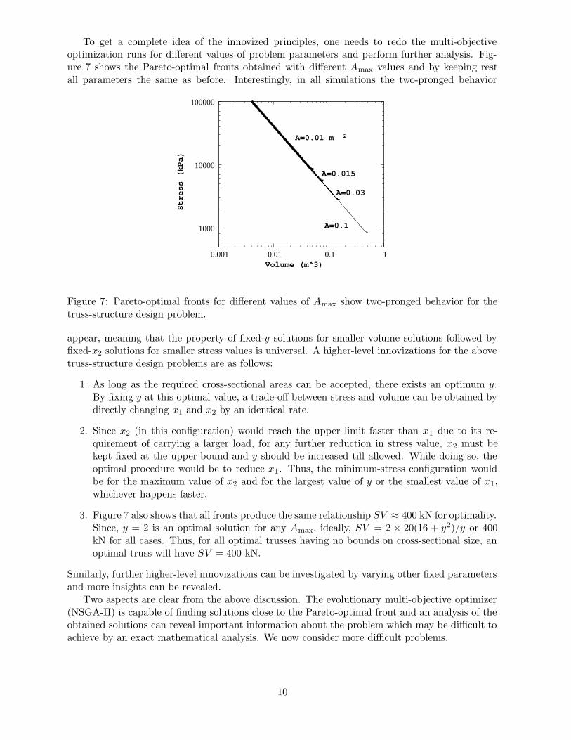
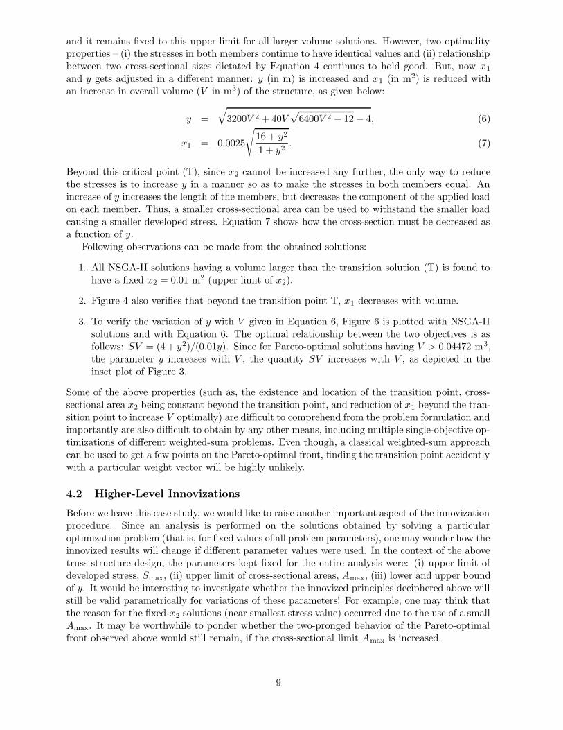
To get a complete idea of the innovized principles, one needs to redo the multi-objectiveoptimization runs for different values of problem parameters and perform further analysis. Fig-ure 7 shows the Pareto-optimal fronts obtained with different Amax values and by keeping restall parameters the same as before. Interestingly, in all simulations the two-pronged behavior

2

1000

10000

100000

0.001 0.01 0.1 1Volume (m^3)

Stress (kPa)

A=0.1

A=0.015

A=0.03

A=0.01 m

Figure 7: Pareto-optimal fronts for different values of Amax show two-pronged behavior for thetruss-structure design problem.

appear, meaning that the property of fixed-y solutions for smaller volume solutions followed byfixed-x2 solutions for smaller stress values is universal. A higher-level innovizations for the abovetruss-structure design problems are as follows:

1. As long as the required cross-sectional areas can be accepted, there exists an optimum y.By fixing y at this optimal value, a trade-off between stress and volume can be obtained bydirectly changing x1 and x2 by an identical rate.

2. Since x2 (in this configuration) would reach the upper limit faster than x1 due to its re-quirement of carrying a larger load, for any further reduction in stress value, x2 must bekept fixed at the upper bound and y should be increased till allowed. While doing so, theoptimal procedure would be to reduce x1. Thus, the minimum-stress configuration wouldbe for the maximum value of x2 and for the largest value of y or the smallest value of x1,whichever happens faster.

3. Figure 7 also shows that all fronts produce the same relationship SV ≈ 400 kN for optimality.Since, y = 2 is an optimal solution for any Amax, ideally, SV = 2 × 20(16 + y2)/y or 400kN for all cases. Thus, for all optimal trusses having no bounds on cross-sectional size, anoptimal truss will have SV = 400 kN.

Similarly, further higher-level innovizations can be investigated by varying other fixed parametersand more insights can be revealed.

Two aspects are clear from the above discussion. The evolutionary multi-objective optimizer(NSGA-II) is capable of finding solutions close to the Pareto-optimal front and an analysis of theobtained solutions can reveal important information about the problem which may be difficult toachieve by an exact mathematical analysis. We now consider more difficult problems.

10

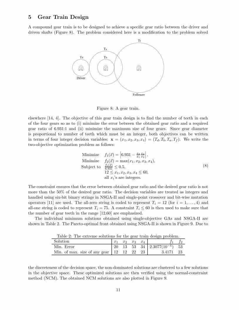
5 Gear Train Design

A compound gear train is to be designed to achieve a specific gear ratio between the driver anddriven shafts (Figure 8). The problem considered here is a modification to the problem solved

������ ������ ������

T Tb

f

d

Ta

Follower

Driver

T

Figure 8: A gear train.

elsewhere [14, 4]. The objective of this gear train design is to find the number of teeth in eachof the four gears so as to (i) minimize the error between the obtained gear ratio and a requiredgear ratio of 6.931:1 and (ii) minimize the maximum size of four gears. Since gear diameteris proportional to number of teeth which must be an integer, both objectives can be writtenin terms of four integer decision variables: x = (x1, x2, x3, x4) = (Td, Tb, Ta, Tf ). We write thetwo-objective optimization problem as follows:

Minimize f1(~x) =∣

∣

∣6.931 − x3

x1

x4

x2

∣

∣

∣ ,

Minimize f2(~x) = max(x1, x2, x3, x4),

Subject to f1(~x)6.931 ≤ 0.5,12 ≤ x1, x2, x3, x4 ≤ 60,all xi’s are integers.

(8)

The constraint ensures that the error between obtained gear ratio and the desired gear ratio is notmore than the 50% of the desired gear ratio. The decision variables are treated as integers andhandled using six-bit binary strings in NSGA-II and single-point crossover and bit-wise mutationoperators [11] are used. The all-zero string is coded to represent Ti = 12 (for i = 1, . . . , 4) andall-one string is coded to represent Ti = 75. A constraint Ti ≤ 60 is then used to make sure thatthe number of gear teeth in the range [12,60] are emphasized.

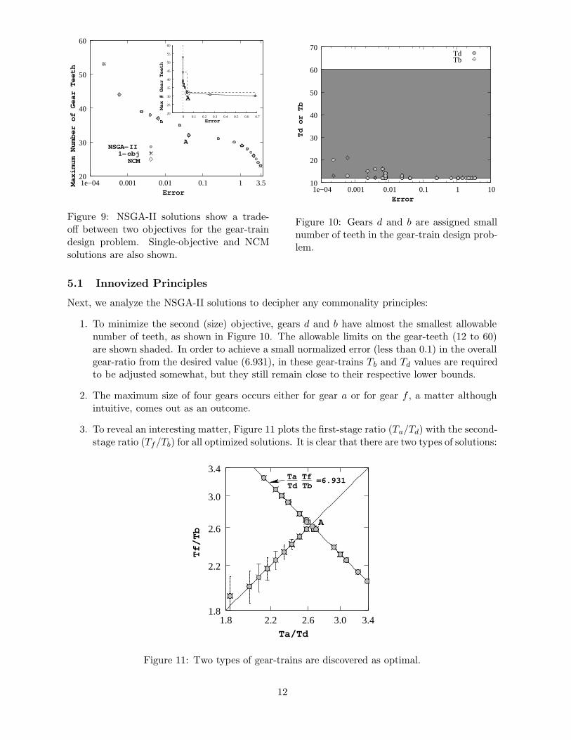
The individual minimum solutions obtained using single-objective GAs and NSGA-II areshown in Table 2. The Pareto-optimal front obtained using NSGA-II is shown in Figure 9. Due to

Table 2: The extreme solutions for the gear train design problem.Solution x1 x2 x3 x4 f1 f2

Min. Error 20 13 53 34 2.3077(10−4) 53Min. of max. size of any gear 12 12 22 23 3.4171 23

the discreteness of the decision space, the non-dominated solutions are clustered to a few solutionsin the objective space. These optimized solutions are then verified using the normal-constraintmethod (NCM). The obtained NCM solutions are also plotted in Figure 9.

11

A

ANSGA−II

1−objNCM

20

30

40

50

60

1e−04 0.001 0.01 0.1 1 3.5Maximum Number of Gear Teeth

Error

20

25

30

35

40

45

50

55

60

0 0.1 0.2 0.3 0.4 0.5 0.6 0.7Error

Max # Gear Teeth

Figure 9: NSGA-II solutions show a trade-off between two objectives for the gear-traindesign problem. Single-objective and NCMsolutions are also shown.

10

20

30

40

50

60

70

1e−04 0.001 0.01 0.1 1 10

TdTb

Error

Td or Tb

Figure 10: Gears d and b are assigned smallnumber of teeth in the gear-train design prob-lem.

5.1 Innovized Principles

Next, we analyze the NSGA-II solutions to decipher any commonality principles:

1. To minimize the second (size) objective, gears d and b have almost the smallest allowablenumber of teeth, as shown in Figure 10. The allowable limits on the gear-teeth (12 to 60)are shown shaded. In order to achieve a small normalized error (less than 0.1) in the overallgear-ratio from the desired value (6.931), in these gear-trains Tb and Td values are requiredto be adjusted somewhat, but they still remain close to their respective lower bounds.

2. The maximum size of four gears occurs either for gear a or for gear f , a matter althoughintuitive, comes out as an outcome.

3. To reveal an interesting matter, Figure 11 plots the first-stage ratio (Ta/Td) with the second-stage ratio (Tf/Tb) for all optimized solutions. It is clear that there are two types of solutions:

A

Ta TfTd Tb

=6.931

Ta/Td

Tf/Tb

1.8 2.2 2.6 3.0 3.41.8

2.2

2.6

3.0

3.4

Figure 11: Two types of gear-trains are discovered as optimal.

12

(i) gear-trains which have very small error (say, less than 0.1), that is, the product of thesecond and first-stage ratios is almost equal to the desired overall ratio (6.931:1) and (ii) gear-trains which have comparatively larger error from the desired gear ratio. Interestingly, forthese latter gear-trains (a vertical error-bar on them indicates the error), both the first andthe second-stage ratios are identical (except the one with the largest error). Although a largeerror can happen for many different combinations of errors in two stages, the minimizationof the second objective (maximum number of gear teeth) causes both stages of gear-ratios tobe identical – a matter which is not quite intuitive, but comes out as an innovized principleto this problem.

4. However, when the error is small (say, less than 0.1), although a gear-train (solution A(12, 12, 32, 31) in the inset plot of Figure 9) with almost identical gear ratios (first stage32/12 = 2.667 and second-stage 31/12 = 2.583) (ideally,

√6.931 = 2.633) exists in the

Pareto-optimal set, there are certainly many other ways (making the product Ta

Td

Tf

Tbalmost

equal to 6.931) to achieve the overall gear ratio, as shown in Figure 11. It is also interestingto note that solution A in Figure 9 is a knee solution. In order to move to neighboringsolutions in either objective, a comparatively larger sacrifice in one objective must be madeto have a small gain in the other objective. From a consideration of both objectives, thissolution would be an ideal choice to a decision-maker and an investigation of the obtainedsolutions also reveals that this solution makes an almost equal distribution of gear-ratiosbetween two stages and also produces a small error in overall gear-ratio from the desiredvalue.

5. In the category of small-error gear-trains, exactly half of them have larger first-stage ratiothan that in the second stage and other half have larger second-stage ratio than that in thefirst stage. This is apparent as the combined gear-ratio of (Ta/Td) · (Tf/Tb) = 6.931 can beachieved for Ta/Td = α and Tf/Tb = β making α · β = 6.931. An identical combined gearratio can also be achieved by swapping the first-stage gears with the second-stage gears,thereby making Ta/Td = β and Tf/Tb = α.

This example, though simple again, brings out a number of interesting properties of a gear-traindesign problem. Importantly, this study also depicts that NSGA-II and other procedures describedhere are also capable to be applied to non-linear integer programming problems.

6 Multiple-Disk Clutch Brake Design

In this problem, a multiple clutch brake [20], as shown in Figure 12, needs to be designed. Twoconflicting objectives are considered: (i) minimization of mass (f1 in kg) of the brake system and(ii) minimization of stopping time (T in s). There are five decision variables: ~x = (ri, ro, t, F, Z),where ri is the inner radius in mm, ro is the outer radius in mm, t is the thickness of discs in mm,F is the actuating force in N and Z is the number of friction surfaces (or discs). All five variablesare considered discrete and their allowable values are given below:

ri = (60, 61, 62, . . . , 78, 79, 80)mm,ro = (90, 91, 92, . . . , 108, 109, 110)mm,t = (1, 1.5, 2, 2.5, 3)mm,F = (600, 610, 620, . . . , 980, 990, 1000)N,Z = (2, 3, 4, 5, 6, 7, 8, 10).

13

���

���

���

���

F r roi

t δ

Figure 12: A multiple-disk clutch brake.

The optimization problem is formulated below:

Minimize f1(~x) = π(x22 − x1

2)x3(x5 + 1)ρ,

Minimize f2(~x) = T = IZωMh+Mf

,

Subject to g1(~x) = x2 − x1 − ∆R ≥ 0,g2(~x) = Lmax − (x5 + 1)(x3 + δ) ≥ 0,g3(~x) = pmax − prz ≥ 0,g4(~x) = pmaxVsr,max − przVsr ≥ 0,g5(~x) = Vsr,max − Vsr ≥ 0,g6(~x) = Mh − sMs ≥ 0,g7(~x) = T ≥ 0,g8(~x) = Tmax − T ≥ 0,ri,min ≤ x1 ≤ ri,max,ro,min ≤ x2 ≤ ro,max,tmin ≤ x3 ≤ tmax,0 ≤ x4 ≤ Fmax,2 ≤ x5 ≤ Zmax.

(9)

The parameters are given below:

Mh = 23µx4x5

x23−x1

3

x22−x1

2 N·mm, ω = πn/30 rad/s, A = π(x22 − x1

2) mm2, prz = x4

A N/mm2,

Vsr = πRsrn30 mm/s, Rsr = 2

3x2

3−x1

3

x22−x1

2 mm, ∆R = 20 mm, Lmax = 30 mm,

µ = 0.5, pmax = 1 MPa, ρ = 0.0000078 kg/mm3, Vsr,max = 10 m/s,s = 1.5, Tmax = 15 s, n = 250 rpm, Ms = 40 Nm,Mf = 3 Nm, Iz = 55 kg·m2, δ = 0.5 mm, ri,min = 60 mm,ri,max = 80 mm, ro,min = 90 mm, ro,min = 110 mm, tmin = 1.5 mm,tmax = 3 mm, Fmax = 1, 000 N, Zmax = 9.

Individual minimum solutions are found by a single-objective NSGA-II and are shown in Table 3.The trade-off between two objectives is clear from the table. The Pareto-optimal front obtainedusing NSGA-II is shown in Figure 13. The extreme solutions shown in the table are also membersof the Pareto-optimal front. The front is also verified by finding a number of optimal solutionsusing the NC method. The two extreme solutions shown in Table 3 are also identical to thosereported elsewhere [20].

6.1 Innovized Principles

Following observations are made by analyzing the NSGA-II results.

14

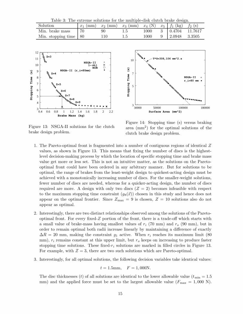
Table 3: The extreme solutions for the multiple-disk clutch brake design.Solution x1 (mm) x2 (mm) x3 (mm) x4 (N) x5 f1 (kg) f2 (s)

Min. brake mass 70 90 1.5 1000 3 0.4704 11.7617Min. stopping time 80 110 1.5 1000 9 2.0948 3.3505

Z=3

Z=4

Z=5

Z=6

Z=7

Z=9Z=8

NSGA−II

3

4

5

6

7

8

9

10

11

12

0.4 0.6 0.8 1 1.2 1.4 1.6 1.8 2 2.2Brake Mass (kg)

Stopping Time (s)

NCM1−obj

NSGA−II (r_i=80mm)

Figure 13: NSGA-II solutions for the clutchbrake design problem.

r_i=80 mmNSGA−II

T*S=308,106 mm^2.s10

7

5

31800001000005000030000

Surface Area (mm^2)

Stopping Time (s)

Figure 14: Stopping time (s) versus brakingarea (mm2) for the optimal solutions of theclutch brake design problem.

1. The Pareto-optimal front is fragmented into a number of contiguous regions of identical Zvalues, as shown in Figure 13. This means that fixing the number of discs is the highest-level decision-making process by which the location of specific stopping time and brake massvalue get more or less set. This is not an intuitive matter, as the solutions on the Pareto-optimal front could have been ordered in any arbitrary manner. But for solutions to beoptimal, the range of brakes from the least-weight design to quickest-acting design must beachieved with a monotonically increasing number of discs. For the smaller-weight solutions,fewer number of discs are needed, whereas for a quicker-acting design, the number of discsrequired are more. A design with only two discs (Z = 2) becomes infeasible with respectto the maximum stopping time constraint (g8(~x)) chosen in this study and hence does notappear on the optimal frontier. Since Zmax = 9 is chosen, Z = 10 solutions also do notappear as optimal.

2. Interestingly, there are two distinct relationships observed among the solutions of the Pareto-optimal front. For every fixed-Z portion of the front, there is a trade-off which starts witha small value of brake-mass having smallest values of ri (70 mm) and ro (90 mm), but inorder to remain optimal both radii increase linearly by maintaining a difference of exactly∆R = 20 mm, making the constraint g1 active. When ri reaches its maximum limit (80mm), ri remains constant at this upper limit, but ro keeps on increasing to produce fasterstopping time solutions. These fixed-ri solutions are marked in filled circles in Figure 13.For example, with Z = 3, there are two such solutions which are Pareto-optimal.

3. Interestingly, for all optimal solutions, the following decision variables take identical values:

t = 1.5mm, F = 1, 000N.

The disc thicknesses (t) of all solutions are identical to the lower allowable value (tmin = 1.5mm) and the applied force must be set to the largest allowable value (Fmax = 1, 000 N).

15

These innovative relationships for an optimal solution is far from being intuitive and canonly be inferred from the obtained optimized data.

4. It is also interesting to note that the stopping time (T) is inversely proportional to the totalbraking area (S) of the system, as shown in Figure 14. Although it may be intuitive toa designer that a quicker stopping time solution is expected to be achieved for a brakingsystem having a larger braking area, NSGA-II solutions bring out an exact relationship(T · S = 308, 106 mm2·s) between the two quantities in this problem. Since the thickness ofthe discs is found to be exactly the same for all optimal solutions, the mass (first objective)and braking surface area are proportional to each other. Figure 13 also shows an inverserelationship between the two objectives. It is also interesting to note that for solutionshaving the inner disc radius more than its allowed upper limit (80 mm), as shown in theFigure 14 with filled circles, the above inverse relationship does not hold.

As indicated above, it is clear from the results that fixing the number of discs is the highest-leveldecision-making in this design process. Say for example, if we need to design a brake systemcapable of stopping in a maximum of 5 seconds, Figure 13 immediately indicates that a minimumof Z = 7 discs are needed with a smallest weight of 0.964 kg, requiring ri = 72 mm and r0 = 92mm. Any optimal design with a particular stopping time T must have an overall surface areaof contact equal to S = 308, 106/T mm2. Moreover, if a brake with a stopping time in therange 4.6 seconds to about 5.1 seconds is required, the optimal design should have seven discswith its weight ranging between 0.941 kg to 1.047 kg. Thus, Figure 13 and the correspondingdecision variables values can be used as a ‘recipe’ of arriving at an optimal design for a particulardesired performance of the braking system. Moreover, the use of the smallest possible thicknessof discs and largest possible applied load would ensure working of the brake system at its optimalperformance.

6.2 Higher-Level Innovizations

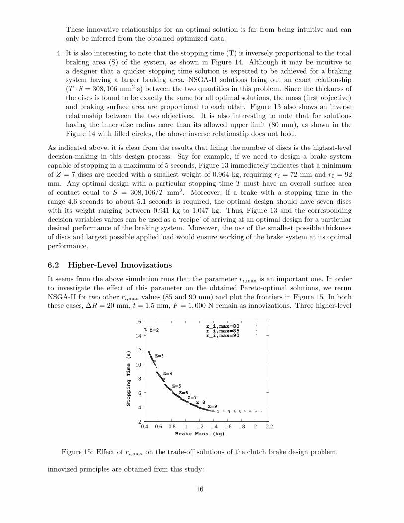
It seems from the above simulation runs that the parameter ri,max is an important one. In orderto investigate the effect of this parameter on the obtained Pareto-optimal solutions, we rerunNSGA-II for two other ri,max values (85 and 90 mm) and plot the frontiers in Figure 15. In boththese cases, ∆R = 20 mm, t = 1.5 mm, F = 1, 000 N remain as innovizations. Three higher-level

Z=2

Z=5Z=6

Z=7Z=8

Z=9

Z=4

Z=3

2

4

6

8

10

12

14

16

0.4 0.6 0.8 1 1.2 1.4 1.6 1.8 2 2.2Brake Mass (kg)

Stopping Time (s)

r_i,max=80r_i,max=85r_i,max=90

Figure 15: Effect of ri,max on the trade-off solutions of the clutch brake design problem.

innovized principles are obtained from this study:

16

1. With larger upper limit of ri, the gap between trade-off fragments of two consecutive Zvalues reduce. Thus, the deviation of optimal solutions (shown with filled circles) from fixedT ·S relationship observed in Figure 14 is purely due to the fixation of the upper limit of ri.

2. Solutions obtained with fixed ri = ri,max are better for a larger ri,max value. However,solutions having ri < ri,max and obtained with different ri,max values all follow the T · S =308, 106 relationship. Thus, the T -S relationship is independent of the choice of ri,max.

3. With larger upper limit of ri, more light-weight brakes with only Z = 2 discs having astopping time less than or equal to 15 seconds are possible. Recall that with ri,max = 80mm, Z = 2 solutions were infeasible. These light-weight brakes have larger ri and ro valuesthan the earlier case, thereby allowing to have a larger surface area per disc.

With the limit of ri,max = 85 or 90 mm, the lightest weight brake weighs 0.4145 kg having ri = 84mm and ro = 104 mm, as opposed to 0.4704 kg obtained with ri,max = 80 mm. Similarly, a quicker-acting brake can be designed with an increase in ri,max (T = 3.20 seconds with ri,max = 90 mmcompared to T = 3.35 seconds with ri,max = 80 mm).

7 Spring Design

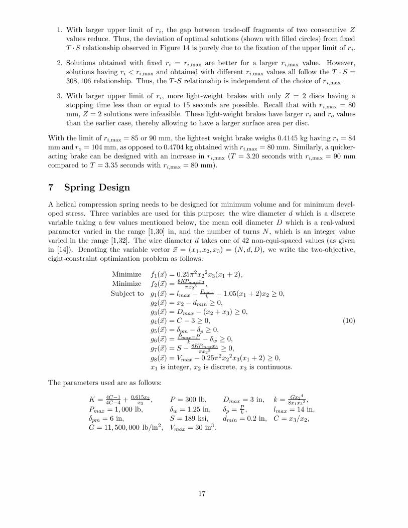
A helical compression spring needs to be designed for minimum volume and for minimum devel-oped stress. Three variables are used for this purpose: the wire diameter d which is a discretevariable taking a few values mentioned below, the mean coil diameter D which is a real-valuedparameter varied in the range [1,30] in, and the number of turns N , which is an integer valuevaried in the range [1,32]. The wire diameter d takes one of 42 non-equi-spaced values (as givenin [14]). Denoting the variable vector ~x = (x1, x2, x3) = (N, d,D), we write the two-objective,eight-constraint optimization problem as follows:

Minimize f1(~x) = 0.25π2x22x3(x1 + 2),

Minimize f2(~x) = 8KPmaxx3

πx23 ,

Subject to g1(~x) = lmax − Pmax

k − 1.05(x1 + 2)x2 ≥ 0,g2(~x) = x2 − dmin ≥ 0,g3(~x) = Dmax − (x2 + x3) ≥ 0,g4(~x) = C − 3 ≥ 0,g5(~x) = δpm − δp ≥ 0,

g6(~x) = Pmax−Pk − δw ≥ 0,

g7(~x) = S − 8KPmaxx3

πx23 ≥ 0,

g8(~x) = Vmax − 0.25π2x22x3(x1 + 2) ≥ 0,

x1 is integer, x2 is discrete, x3 is continuous.

(10)

The parameters used are as follows:

K = 4C−14C−4 + 0.615x2

x3, P = 300 lb, Dmax = 3 in, k = Gx2

4

8x1x33 ,

Pmax = 1, 000 lb, δw = 1.25 in, δp = Pk , lmax = 14 in,

δpm = 6 in, S = 189 ksi, dmin = 0.2 in, C = x3/x2,G = 11, 500, 000 lb/in2, Vmax = 30 in3.

17

The 42 discrete values of d are given below:

d =

0.009, 0.0095, 0.0104, 0.0118, 0.0128, 0.0132,0.014, 0.015, 0.0162, 0.0173, 0.018, 0.020,0.023, 0.025, 0.028, 0.032, 0.035, 0.041,0.047, 0.054, 0.063, 0.072, 0.080, 0.092,0.105, 0.120, 0.135, 0.148, 0.162, 0.177,0.192, 0.207, 0.225, 0.244, 0.263, 0.283,0.307, 0.331, 0.362, 0.394, 0.4375, 0.5.

The design variables d and D are treated as real-valued parameters in the NSGA-II with d takingdiscrete values from the above set and N is treated with a five-bit binary string, thereby codingintegers in the range [1,32]. While SBX and polynomial mutation operators are used to handle dand D, a single-point crossover and bit-wise mutation are used to handle N .

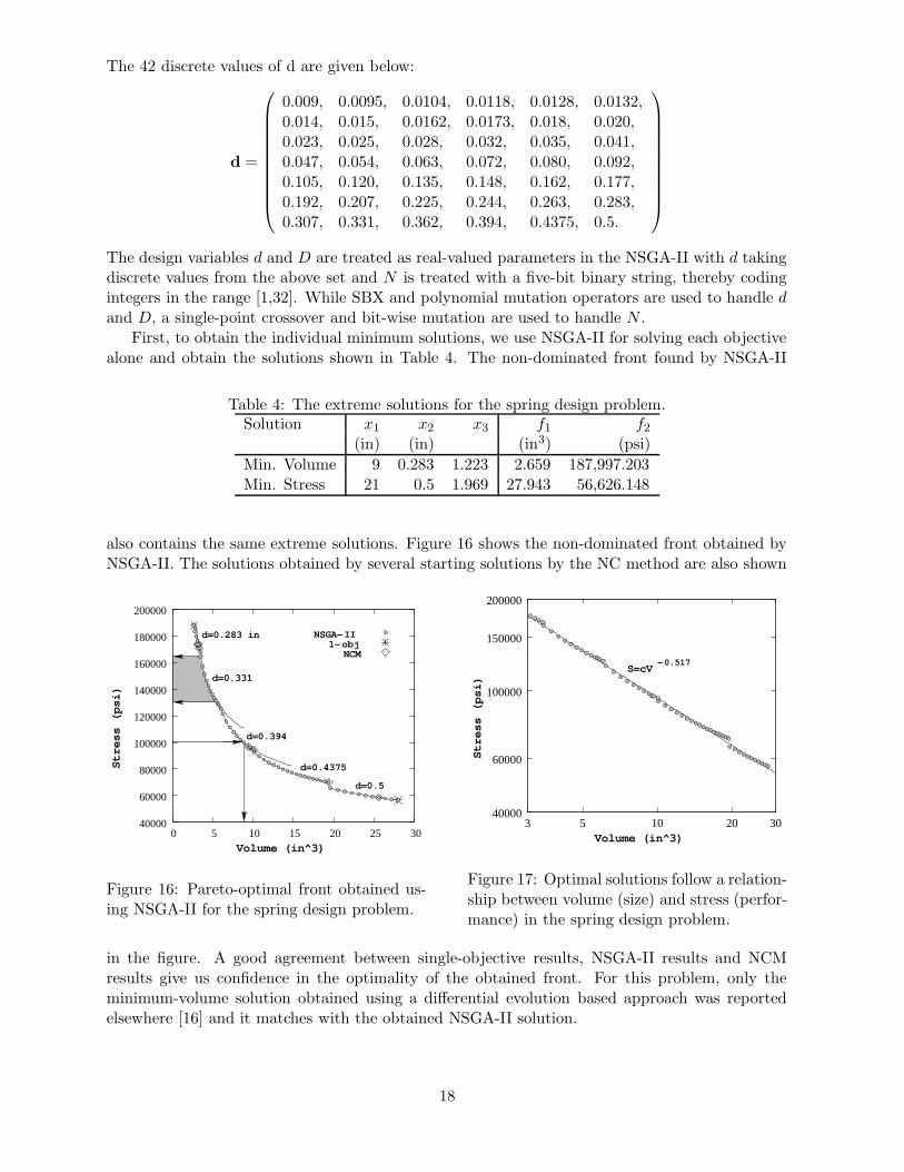
First, to obtain the individual minimum solutions, we use NSGA-II for solving each objectivealone and obtain the solutions shown in Table 4. The non-dominated front found by NSGA-II

Table 4: The extreme solutions for the spring design problem.Solution x1 x2 x3 f1 f2

(in) (in) (in3) (psi)

Min. Volume 9 0.283 1.223 2.659 187,997.203Min. Stress 21 0.5 1.969 27.943 56,626.148

also contains the same extreme solutions. Figure 16 shows the non-dominated front obtained byNSGA-II. The solutions obtained by several starting solutions by the NC method are also shown

d=0.394

d=0.331

d=0.283 in

d=0.4375

d=0.5

NCM1−obj

NSGA−II

30 25 20 15 10 5 0 40000

60000

80000

100000

120000

140000

160000

180000

200000

Volume (in^3)

Stress (psi)

Figure 16: Pareto-optimal front obtained us-ing NSGA-II for the spring design problem.

S=cV−0.517

200000

150000

100000

60000

4000030201053

Stress (psi)

Volume (in^3)

Figure 17: Optimal solutions follow a relation-ship between volume (size) and stress (perfor-mance) in the spring design problem.

in the figure. A good agreement between single-objective results, NSGA-II results and NCMresults give us confidence in the optimality of the obtained front. For this problem, only theminimum-volume solution obtained using a differential evolution based approach was reportedelsewhere [16] and it matches with the obtained NSGA-II solution.

18

7.1 Innovized Principles

Let us now analyze the optimal solutions to find if there are any innovized principles which canbe gathered about the spring design problem. We observe the following principles:

1. The Pareto-optimal front is fragmented and every fragment corresponds to a fixed value ofwire diameter d, as shown in Figure 16. Of 42 different allowed d values, only five valuesmake their places on the Pareto-optimal frontier. Here, fixing the d value fixes the rangeof optimal objective values on the Pareto-optimal frontier, thereby making the selection ofthis parameter the most important decision-making task in the design process.

2. Moreover, not every combination of D and N turns out to be optimal for these five valuesof d. Figure 16 also shows (with a solid line) the complete non-dominated front obtained bykeeping d constant and using only D and N as decision variables. As evident from the figure,some part of each front does not qualify (gets dominated by members of other fragments)to remain as Pareto-optimal when all d values are allowed.

3. For an optimal solution having a small volume, a small d must be chosen. However, thesmallest available wire diameter (d = 0.009 in) is not an optimal choice. In fact, the smallestoptimal wire diameter is d = 0.283 in.

4. When the non-dominated solutions are plotted in a logarithmic scale (Figure 17), optimalobjective values (volume (V ) and stress (S)) are found to have an interesting relationship:SV 0.517 = constant.

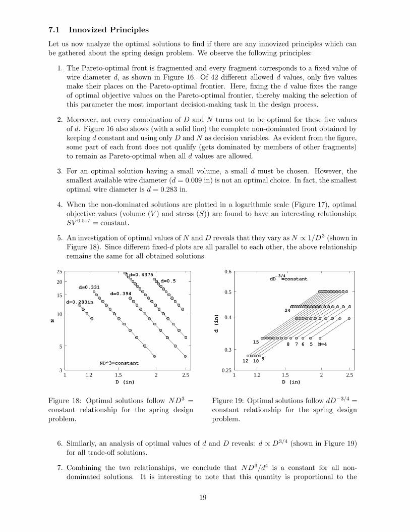
5. An investigation of optimal values of N and D reveals that they vary as N ∝ 1/D3 (shown inFigure 18). Since different fixed-d plots are all parallel to each other, the above relationshipremains the same for all obtained solutions.

d=0.283in

d=0.331d=0.394

d=0.4375d=0.5

ND^3=constant

25

20

15

10

5

32.521.51.21

N

D (in)

Figure 18: Optimal solutions follow ND3 =constant relationship for the spring designproblem.

N=457 68

12

24

910

15

−3/4dD =constant

0.6

0.5

0.4

0.3

0.252.521.51.21

d (in)

D (in)

Figure 19: Optimal solutions follow dD−3/4 =constant relationship for the spring designproblem.

6. Similarly, an analysis of optimal values of d and D reveals: d ∝ D3/4 (shown in Figure 19)for all trade-off solutions.

7. Combining the two relationships, we conclude that ND3/d4 is a constant for all non-dominated solutions. It is interesting to note that this quantity is proportional to the

19

inverse of spring constant k = Gd4/(8ND3). By substituting the constant derived fromthe NSGA-II solutions, we obtain k = 560 lb/in for all optimal solutions. This reveals aninnovation for this spring design problem. In order to create an optimal solution, we simplyneed to have a spring with a fixed spring constant of 560 lb/in for the chosen parametersof the design problem. Obviously, one can have different combinations of d, D and N toachieve this magical spring constant value. Figure 16 shows all such solutions which willmake a non-dominated optimal combination of two objectives. To design an optimal springhaving a small volume (or weight), the spring must be formed using a small sized wire,a small mandrel diameter and a few number of turns. Interestingly, a bigger-sized springcan also be designed with an identical spring constant by having a large sized wire, a largemandrel diameter and a large number of turns. The latter design, although has an identicalspring constant to the former light-weight spring, will be able to withstand a larger amountof stress. What we have achieved with the proposed innovization procedure is a ‘recipe’ toarrive at different trade-off solutions (between size and strength), each having an identicalspring constant of 560 lb/in, but having differing dimensions.

8. Another interesting aspect of the obtained NSGA-II solutions is that the constraint g6 isactive for all solutions. By substituting the fixed parameters in the mathematical constraintfunction (g6), we obtain k = (1000 − 300)/1.25 = 560 lb/in, thereby explaining the specificvalue of the spring constant observed in the obtained data above. Since no other constraintsare active for all Pareto-optimal solutions, other constraints do not result in any otherinnovization.

The above innovized principles provide us with a recipe of designing a spring optimally. Forexample, if a spring has to be designed with a material having yield strength of 100,000 psi,Figure 16 clearly shows that an optimal design must be made from a wire of diameter d = 0.394in. Other design variables must take D = 1.779 in and N = 11 turns and the spring will havea volume of 8.857 in3. The results can also be interpreted as follows. If the designer is lookingfor designing a range of springs with materials having yield strength ranging from 130,000 psi to165,000 psi, the optimal spring must be made from a wire of diameter 0.331 in, thereby requiringto maintain a small inventory for storing only one-sized wires for making optimal springs. Whatis also important here to note that all such springs will be optimal from a dual consideration ofvolume (size) and strength (performance). The information about specific wire diameters (onlyfive out of chosen 42 different values) for optimality and a common property of having a fixed springconstant (of 560 lb/in) are all innovations, which will be difficult to arrive at, otherwise. In thisparticular problem, the chosen value of parameters G, Pmax, P , and δw allowed these propertiesto emerge as innovations for a solution to be optimal. For some other parameter setting, someother innovized principles may have been evolved. But to find such important principles of design,our proposed methodology can be applied again (discussed in the next subsection) and it is notclear how else such vital and useful information about a problem can be learned by any othertechnique.

7.2 Higher-Level Innovizations

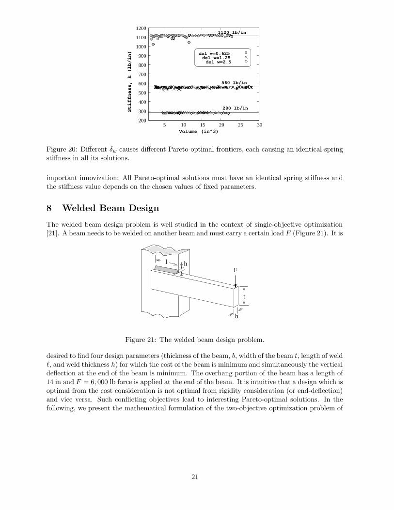
Next, we increase δw to twice to its previous value, that is, we set δw = 2.5 in. When we redothe proposed innovization procedure, we once again observe that the constraint g6 is active forall solutions. Substituting other parameters, we then obtain k = (1000 − 300)/2.5 = 280 lb/in,half of what was achieved previously. Substituting the new values of the design variables in thestiffness term k, we observe that all solutions possess more or less an identical k = 280 lb/in, ascan also be seen from Figure 20. We repeat the study for δw = 0.625 in and observe that thecorresponding stiffness of solutions come close to k = 1, 120 lb/in. This clearly brings out an

20

1120 lb/in

560 lb/in

280 lb/in

200

300

400

500

600

700

800

900

1000

1100

1200

5 10 15 20 25 30

del w=0.625del w=1.25del w=2.5

Volume (in^3)Stiffness, k (lb/in)

Figure 20: Different δw causes different Pareto-optimal frontiers, each causing an identical springstiffness in all its solutions.

important innovization: All Pareto-optimal solutions must have an identical spring stiffness andthe stiffness value depends on the chosen values of fixed parameters.

8 Welded Beam Design

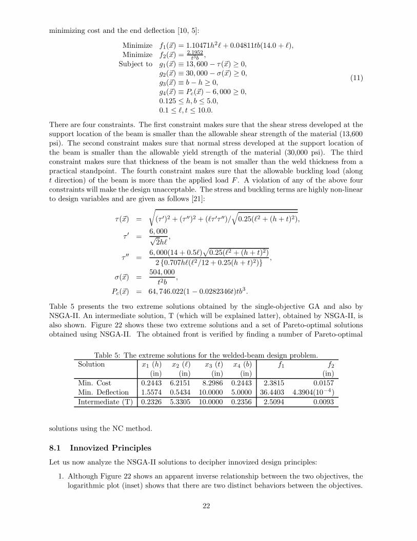
The welded beam design problem is well studied in the context of single-objective optimization[21]. A beam needs to be welded on another beam and must carry a certain load F (Figure 21). It is

b

t

hlF

Figure 21: The welded beam design problem.

desired to find four design parameters (thickness of the beam, b, width of the beam t, length of weld`, and weld thickness h) for which the cost of the beam is minimum and simultaneously the verticaldeflection at the end of the beam is minimum. The overhang portion of the beam has a length of14 in and F = 6, 000 lb force is applied at the end of the beam. It is intuitive that a design which isoptimal from the cost consideration is not optimal from rigidity consideration (or end-deflection)and vice versa. Such conflicting objectives lead to interesting Pareto-optimal solutions. In thefollowing, we present the mathematical formulation of the two-objective optimization problem of

21

minimizing cost and the end deflection [10, 5]:

Minimize f1(~x) = 1.10471h2` + 0.04811tb(14.0 + `),Minimize f2(~x) = 2.1952

t3b ,Subject to g1(~x) ≡ 13, 600 − τ(~x) ≥ 0,

g2(~x) ≡ 30, 000 − σ(~x) ≥ 0,g3(~x) ≡ b − h ≥ 0,g4(~x) ≡ Pc(~x) − 6, 000 ≥ 0,0.125 ≤ h, b ≤ 5.0,0.1 ≤ `, t ≤ 10.0.

(11)

There are four constraints. The first constraint makes sure that the shear stress developed at thesupport location of the beam is smaller than the allowable shear strength of the material (13,600psi). The second constraint makes sure that normal stress developed at the support location ofthe beam is smaller than the allowable yield strength of the material (30,000 psi). The thirdconstraint makes sure that thickness of the beam is not smaller than the weld thickness from apractical standpoint. The fourth constraint makes sure that the allowable buckling load (alongt direction) of the beam is more than the applied load F . A violation of any of the above fourconstraints will make the design unacceptable. The stress and buckling terms are highly non-linearto design variables and are given as follows [21]:

τ(~x) =

√

(τ ′)2 + (τ ′′)2 + (`τ ′τ ′′)/√

0.25(`2 + (h + t)2),

τ ′ =6, 000√

2h`,

τ ′′ =6, 000(14 + 0.5`)

√

0.25(`2 + (h + t)2)

2 {0.707h`(`2/12 + 0.25(h + t)2)} ,

σ(~x) =504, 000

t2b,

Pc(~x) = 64, 746.022(1 − 0.0282346t)tb3 .

Table 5 presents the two extreme solutions obtained by the single-objective GA and also byNSGA-II. An intermediate solution, T (which will be explained latter), obtained by NSGA-II, isalso shown. Figure 22 shows these two extreme solutions and a set of Pareto-optimal solutionsobtained using NSGA-II. The obtained front is verified by finding a number of Pareto-optimal

Table 5: The extreme solutions for the welded-beam design problem.Solution x1 (h) x2 (`) x3 (t) x4 (b) f1 f2

(in) (in) (in) (in) (in)

Min. Cost 0.2443 6.2151 8.2986 0.2443 2.3815 0.0157Min. Deflection 1.5574 0.5434 10.0000 5.0000 36.4403 4.3904(10−4)

Intermediate (T) 0.2326 5.3305 10.0000 0.2356 2.5094 0.0093

solutions using the NC method.

8.1 Innovized Principles

Let us now analyze the NSGA-II solutions to decipher innovized design principles:

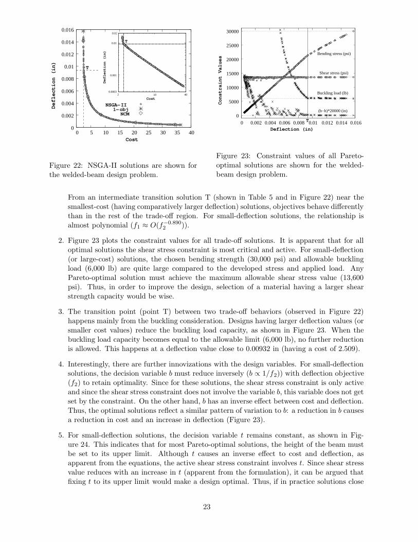
1. Although Figure 22 shows an apparent inverse relationship between the two objectives, thelogarithmic plot (inset) shows that there are two distinct behaviors between the objectives.

22

T

T

NSGA−II1−obj

NCM

0

0.002

0.004

0.006

0.008

0.01

0.012

0.014

0.016

0 5 10 15 20 25 30 35 40Cost

Deflection (in)

0.001

0.01

10 0.0003

0.02

2 40

Cost

Deflection (in)

Figure 22: NSGA-II solutions are shown forthe welded-beam design problem.

T 0

5000

10000

15000

20000

25000

30000

0 0.002 0.004 0.006 0.008 0.01 0.012 0.014 0.016

Bending stress (psi)

Shear stress (psi)

Buckling load (lb)

(b−h)*20000 (in)

Deflection (in)

Constraint Values

Figure 23: Constraint values of all Pareto-optimal solutions are shown for the welded-beam design problem.

From an intermediate transition solution T (shown in Table 5 and in Figure 22) near thesmallest-cost (having comparatively larger deflection) solutions, objectives behave differentlythan in the rest of the trade-off region. For small-deflection solutions, the relationship isalmost polynomial (f1 ≈ O(f−0.890

2 )).

2. Figure 23 plots the constraint values for all trade-off solutions. It is apparent that for alloptimal solutions the shear stress constraint is most critical and active. For small-deflection(or large-cost) solutions, the chosen bending strength (30,000 psi) and allowable bucklingload (6,000 lb) are quite large compared to the developed stress and applied load. AnyPareto-optimal solution must achieve the maximum allowable shear stress value (13,600psi). Thus, in order to improve the design, selection of a material having a larger shearstrength capacity would be wise.

3. The transition point (point T) between two trade-off behaviors (observed in Figure 22)happens mainly from the buckling consideration. Designs having larger deflection values (orsmaller cost values) reduce the buckling load capacity, as shown in Figure 23. When thebuckling load capacity becomes equal to the allowable limit (6,000 lb), no further reductionis allowed. This happens at a deflection value close to 0.00932 in (having a cost of 2.509).

4. Interestingly, there are further innovizations with the design variables. For small-deflectionsolutions, the decision variable b must reduce inversely (b ∝ 1/f2)) with deflection objective(f2) to retain optimality. Since for these solutions, the shear stress constraint is only activeand since the shear stress constraint does not involve the variable b, this variable does not getset by the constraint. On the other hand, b has an inverse effect between cost and deflection.Thus, the optimal solutions reflect a similar pattern of variation to b: a reduction in b causesa reduction in cost and an increase in deflection (Figure 23).

5. For small-deflection solutions, the decision variable t remains constant, as shown in Fig-ure 24. This indicates that for most Pareto-optimal solutions, the height of the beam mustbe set to its upper limit. Although t causes an inverse effect to cost and deflection, asapparent from the equations, the active shear stress constraint involves t. Since shear stressvalue reduces with an increase in t (apparent from the formulation), it can be argued thatfixing t to its upper limit would make a design optimal. Thus, if in practice solutions close

23

t(in)

b(in)

T 0.0004 0.001 0.01 0.1

0.125

1

5

10

0.02Deflection (in)

t or b (in)

Figure 24: Variations of design variables t andb across the Pareto-optimal front are shownfor the welded-beam design problem.

l(in)

h(in)

T

Deflection (in)

h or l (in)

0.1 0.125

0.0004 0.001 0.01 0.02

1

5

10

Figure 25: Variations of design variables h and` across the Pareto-optimal front are shownfor the welded-beam design problem.

to the smallest-cost solution are not desired, a beam of identical height (t = 10 in) may onlybe procured, thereby simplifying the inventory.

6. However, an increase of ` and a decrease in h with an increase in deflection (or a decreasein cost) are not completely monotonic, as can be seen from Figure 25. These two phenom-ena are not at all intuitive and are also difficult to explain from the problem formulation.However, the innovized principles for arriving at optimal solutions seem to be as follows:for a reduced cost solution, keep t fixed to its upper limit, increase ` and reduce h and b.This ‘recipe’ of design can be practiced only till the applied load is strictly smaller than theallowable buckling load.

7. Thereafter, any reduction in cost optimally must come from (i) reducing t from its upperlimit, (ii) increasing b, and (iii) adjusting other two variables so as to make buckling, shearstress, and constraint g4 active. In these solutions, with decreasing cost, the dimensions arereduced in such a manner so as to make the bending stress to increase. Finally, the minimumcost solution occurs when the bending stress equals to the allowable strength (30,000 psi, asin Figure 23). At this solution all four constraints become active, so as to optimally utilizethe materials for all four purposes.

8. To achieve very small cost solutions, the innovized principles are different: for a reducedcost solution, reduce t and increase `, h and b. Thus, overall a larger ` is needed to achievea small cost solution.

8.2 Higher-Level Innovizations

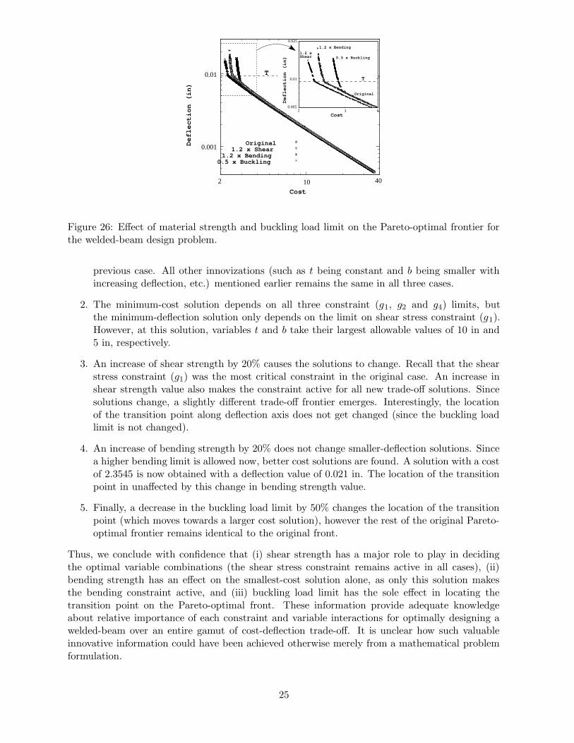
Here, we redo the innovization procedure for one different value of three allowable limits: shearstrength in constraint g1 is increased by 20%, bending strength in constraint g2 is increased by20%, and buckling limit load in constraint g4 is reduced by 50%. We change them one at a time andkeep the other parameters identical to their previous values. Figure 26 shows the correspondingPareto-optimal frontiers for these three cases. Following innovizations are obtained:

1. It is clear that all three cases produce similar dual behavior (different characteristics oneither side of a transition point) in the Pareto-optimal frontier, as was also observed in the

24

Original

0.5 x Buckling

1.2 x Bending

Shear1.2 x

TT

Deflection (in)

0.01

0.005

0.025

2 3 4Cost

0.5 x Buckling1.2 x Bending

1.2 x ShearOriginal

CostDeflection (in)

0.001

0.01

10 2 40

Figure 26: Effect of material strength and buckling load limit on the Pareto-optimal frontier forthe welded-beam design problem.

previous case. All other innovizations (such as t being constant and b being smaller withincreasing deflection, etc.) mentioned earlier remains the same in all three cases.

2. The minimum-cost solution depends on all three constraint (g1, g2 and g4) limits, butthe minimum-deflection solution only depends on the limit on shear stress constraint (g1).However, at this solution, variables t and b take their largest allowable values of 10 in and5 in, respectively.

3. An increase of shear strength by 20% causes the solutions to change. Recall that the shearstress constraint (g1) was the most critical constraint in the original case. An increase inshear strength value also makes the constraint active for all new trade-off solutions. Sincesolutions change, a slightly different trade-off frontier emerges. Interestingly, the locationof the transition point along deflection axis does not get changed (since the buckling loadlimit is not changed).

4. An increase of bending strength by 20% does not change smaller-deflection solutions. Sincea higher bending limit is allowed now, better cost solutions are found. A solution with a costof 2.3545 is now obtained with a deflection value of 0.021 in. The location of the transitionpoint in unaffected by this change in bending strength value.

5. Finally, a decrease in the buckling load limit by 50% changes the location of the transitionpoint (which moves towards a larger cost solution), however the rest of the original Pareto-optimal frontier remains identical to the original front.

Thus, we conclude with confidence that (i) shear strength has a major role to play in decidingthe optimal variable combinations (the shear stress constraint remains active in all cases), (ii)bending strength has an effect on the smallest-cost solution alone, as only this solution makesthe bending constraint active, and (iii) buckling load limit has the sole effect in locating thetransition point on the Pareto-optimal front. These information provide adequate knowledgeabout relative importance of each constraint and variable interactions for optimally designing awelded-beam over an entire gamut of cost-deflection trade-off. It is unclear how such valuableinnovative information could have been achieved otherwise merely from a mathematical problemformulation.

25

9 Conclusions

In this paper, we have introduced a new design procedure (through a new terminology, we called’innovization procedure’) based on multi-objective optimization and a post-optimality analysis ofoptimized solutions. We have argued that the task of a single-objective optimization results ina single optimum solution which may not provide enough information about useful relationshipsamong design variables, constraints and objectives for achieving different trade-off solutions. Onthe other hand, consideration of at least two conflicting objectives of design should result ina number of optimal solutions, trading-off the two objectives. Thereafter, a post-optimalityanalysis of these optimal solutions should provide useful information and design principles aboutthe problem, such as relationships among variables and objectives which are common among theoptimal solutions and the differences which make the optimal solutions different from each other.We have argued that such information should often introduce new principles for optimal designs,thereby allowing designers to learn innovations about solving the problem at hand.

On a number of engineering design problems having mixed discrete and continuous designvariables, many useful innovizations (innovative design principles) are deciphered. Interestingly,many such innovizations were not intuitive and not known before. The ease of application ofthe proposed innovization procedure has also become clear from different applications. It is alsoclear that the proposed procedure is useful and ready to be used in other more complex designtasks. The procedure will enable designers to perform the innovization task once and for all tothe problem at hand and the knowledge thus gained will go a long way in understanding theintricacies of the problems and in solving such future design tasks. On another note, since thePareto-optimal frontier obtained using NSGA-II are verified by other single-objective optimizationtechniques, the reported trade-off solutions also remain as ‘benchmark’ optimal solutions to theseproblems.

However, the innovization procedure suggested here must now be made more automatic andproblem-independent as far as possible. In this regard, an efficient data-mining technique is inorder to evolve innovative design relationships from the Pareto-optimal solutions. Although someapparent hurdles of this task have been pointed out in this paper, effort is underway at KanpurGenetic Algorithms Laboratory (KanGAL) in this direction.

Finally, it is also worth mentioning that similar to the expectation of common propertiesto exist among Pareto-optimal solutions (as discovered and demonstrated amply in this paper),commonality principles may also be expected to exist in other kinds of trade-off solutions, suchas among weakly Pareto-optimal solutions, locally Pareto-optimal solutions [6], and robust orreliable Pareto-optimal solutions [9]. It would be interesting then to investigate how the innovizedrelationships get changed from one type of optimal solutions to the other. For example, suchan analysis may provide answers to questions such as how are robust Pareto-optimal solutionsdifferent from the Pareto-optimal solutions themselves! Another interesting extension of thisstudy would be to consider three or more conflicting objectives of design and a resulting post-optimality analysis may yield higher-level innovizations than that may be obtained with thetwo-objective procedure. The ease and ability of NSGA-II to handle different vagaries of designvariables (discrete, Boolean, real-valued etc.), nonlinearities in constraint and objective functions,scalability in problem size, and multi-modality and multi-objectivity in problem formulationsallow such an innovization task tractable and worth performing.

References

[1] H. P. Benson. Existence of efficient solutions for vector maximization problems. Journal ofOptimization Theory and Applications, 26(4):569–580, 1978.

26

[2] V. Chankong and Y. Y. Haimes. Multiobjective Decision Making Theory and Methodology.New York: North-Holland, 1983.

[3] C. A. C. Coello, D. A. VanVeldhuizen, and G. Lamont. Evolutionary Algorithms for SolvingMulti-Objective Problems. Boston, MA: Kluwer Academic Publishers, 2002.

[4] K. Deb. Mechanical component design using genetic algorithms. In D. Dasgupta andZ. Michalewicz, editors, Evolutionary Algorithms in Engineering Applications, pages 495–512. New York: Springer-Verlag, 1997.

[5] K. Deb. An efficient constraint handling method for genetic algorithms. Computer Methodsin Applied Mechanics and Engineering, 186(2–4):311–338, 2000.

[6] K. Deb. Multi-objective optimization using evolutionary algorithms. Chichester, UK: Wiley,2001.

[7] K. Deb. Unveiling innovative design principles by means of multiple conflicting objectives.Engineering Optimization, 35(5):445–470, 2003.

[8] K. Deb, S. Agrawal, A. Pratap, and T. Meyarivan. A fast and elitist multi-objective geneticalgorithm: NSGA-II. IEEE Transactions on Evolutionary Computation, 6(2):182–197, 2002.

[9] K. Deb and H. Gupta. Searching for robust Pareto-optimal solutions in multi-objectiveoptimization. In Proceedings of the Third Evolutionary Multi-Criteria Optimization (EMO-05) Conference (Also Lecture Notes on Computer Science 3410), pages 150–164, 2005.

[10] K. Deb and A. Kumar. Real-coded genetic algorithms with simulated binary crossover:Studies on multi-modal and multi-objective problems. Complex Systems, 9(6):431–454, 1995.

[11] D. E. Goldberg. Genetic Algorithms for Search, Optimization, and Machine Learning. Read-ing, MA: Addison-Wesley, 1989.

[12] D. E. Goldberg. The design of innovation: Lessons from and for Competent genetic algo-rithms. Kluwer Academic Publishers, 2002.

[13] J. Jahn. Vector optimization. Berlin, Germany: Springer-Verlag, 2004.

[14] B. K. Kannan and S. N. Kramer. An augmented lagrange multiplier based method for mixedinteger discrete continuous optimization and its applications to mechanical design. ASMEJournal of Mechanical Design, 116(2):405–411, 1994.

[15] P. Korhonen, S. Salo, and R. Steuer. A heuristic for estimating nadir criterion values inmultiple objective linear programming. Operations Research, 45(5):751–757, 1997.

[16] J. Lampinen and I. Zelinka. Mechanical engineering design optimization by differential evo-lution. In D. Corne, M. Dorigo, and F. Glover, editors, New Ideas in Optimization, pages127–146. Berkshire, UK: McGraw-Hill, 1999.

[17] Siemens Ltd. TEFC 3 phase squirrel cage induction motor catalogue,http://globaludyog.com/pumps/sl.htm.

[18] A. Messac and C. A. Mattson. Normal constraint method with guarantee of even represen-tation of complete pareto frontier. AIAA Journal, in press.

[19] K. Miettinen. Nonlinear Multiobjective Optimization. Kluwer, Boston, 1999.

27

[20] A. Osyczka. Evolutionary algorithms for single and multicriteria design optimization. Hei-delberg: Physica-Verlag, 2002.

[21] G. V. Reklaitis, A. Ravindran, and K. M. Ragsdell. Engineering Optimization Methods andApplications. New York : Wiley, 1983.

28