Innovations of wide-field optical-sectioning fluorescencemicroscopy: toward high-speed volumetric bio-imaging with

simplicity

Thesis by

Jiun-Yann Yu

In Partial Fulfillment of the Requirements

for the Degree of

Doctor of Philosophy

California Institute of Technology

Pasadena, California

2014

(Defended March 25, 2014)

ii

c© 2014

Jiun-Yann Yu

All Rights Reserved

iii

Acknowledgements

Firstly, I would like to thank my thesis advisor, Professor Chin-Lin Guo, for all of his kind advice and

generous financial support during these five years. I would also like to thank all of the faculties in my

thesis committee: Professor Geoffrey A. Blake, Professor Scott E. Fraser, and Professor Changhuei

Yang, for their guidance on my way towards becoming a scientist. I would like to specifically

thank Professor Blake, and his graduate student, Dr. Daniel B. Holland, for their endless kindness,

enthusiasms and encouragements with our collaborations, without which there would be no more

than 10 pages left in this thesis. Dr. Thai Truong of Prof. Fraser’s group and Marco A. Allodi of

Professor Blake’s group are also sincerely acknowledged for contributing to this collaboration.

All of the members of Professor Guo’s group at Caltech are gratefully acknowledged. I would

like to thank our former postdoctoral scholar Dr. Yenyu Chen for generously teaching me all the

engineering skills I need, and passing to me his pursuit of wide-field optical-sectioning microscopy. I

also thank Dr. Mingxing Ouyang for introducing me the basic concepts of cell biology and showing

me the basic techniques of cell-biology experiments. I would like to pay my gratefulness to our

administrative assistant, Lilian Porter, not only for her help on administrative procedures, but also

for her advice and encouragement on my academic career in the future.

Here I thank Dr. Ruben Zadoyan and his former group member Dr. Chun-Hung Kuo for our

collaboration on the project of diffuser-based temporal focusing. I would like to thank Professor

Young-Geun Han and his group members Sunduck Kim and Young Bo Shim at Hanyang University

who made the fiber-illumination project possible. Professor Wonhee Lee and his group member

Jonghyun Kim at Korea Advanced Institute of Science and Technology are gratefully acknowledged

for developing the prototype of the height-staggered plates. My sincere acknowledgment also goes to

iv

Professor Paul Sternberg and his group member Hui Chiu, who kindly helped me prepared C. elegans

of several different lines for imaging. Meanwhile, I would like to thank Dr. Chao-Yuan Yeh for his

advice on choosing appropriate biological samples, and Yun Mou for his advice on using appropriate

fluorescent dyes that facilitated axial response measurements. Special thanks to my friends Yu-Hang

Chen for his assistance in computation, and Dr. Chien-Cheng Chen for his inspiring suggestions on

my research works.

I would like to acknowledge Dr. Alexander Egner for his inspiring instructions with the theoret-

ical calculations in this Thesis. I can’t thank Professor Shi-Wei Chu at National Taiwan University

enough for training me with the basic knowledge and experimental skills of imaging optics, and

helping me pave the way to continue my research of optical microscopy at Caltech. I thank Pro-

fessor Carol J. Cogswell at University of Colorado, Boulder for being a role model for me and for

encouraging me to continue my research approach in developing simple, useful, and cost-efficient

microscopy techniques.

I sincerely acknowledge all of the administrative staffs of Bioengineering option, especially Linda

Scott, for helping me with all the administrative procedures during these years.

I would like to specifically thank my friends Yun Mou, Dr. Chao-Yuan Yeh and Mike (Miroslav)

Vondrus, for their company and endless support on good days and bad days. I gratefully thank Chan

U Lei, Tong Chen, Hao Chu, Hui-Chen Chen, Myoung-Gyun Suh, Wai Chung Wong, Hsiu-Ping Lee,

and Tzu-Chin Chen for our friendship.

There are no words that I can find to express my thankfulness properly to my parents, Jen-Hui

Hsieh and An-Chi Yu; they supported me with no hesitations and no matter how far I deviated

from the route they planned for me. I also thank my sister Chao-Wei Yu and my brother-in-law

Bei-Jiang Lin for their warm, continuing greetings during my good times and bad times, and I wish

that their newborn baby, also my nephew, Tzu-Yang Lin, have a wonderful adventure of life ahead

of him. At last, I would like to acknowledge Wen-Hsuan Chan, who had been my strongest support

in the past ten years.

v

Abstract

Optical microscopy has become an indispensable tool for biological researches since its invention,

mostly owing to its sub-cellular spatial resolutions, non-invasiveness, instrumental simplicity, and the

intuitive observations it provides. Nonetheless, obtaining reliable, quantitative spatial information

from conventional wide-field optical microscopy is not always intuitive as it appears to be. This is

because in the acquired images of optical microscopy the information about out-of-focus regions is

spatially blurred and mixed with in-focus information. In other words, conventional wide-field optical

microscopy transforms the three-dimensional spatial information, or volumetric information about

the objects into a two-dimensional form in each acquired image, and therefore distorts the spatial

information about the object. Several fluorescence holography-based methods have demonstrated

the ability to obtain three-dimensional information about the objects, but these methods generally

rely on decomposing stereoscopic visualizations to extract volumetric information and are unable to

resolve complex 3-dimensional structures such as a multi-layer sphere.

The concept of optical-sectioning techniques, on the other hand, is to detect only two-dimensional

information about an object at each acquisition. Specifically, each image obtained by optical-

sectioning techniques contains mainly the information about an optically thin layer inside the object,

as if only a thin histological section is being observed at a time. Using such a methodology, obtaining

undistorted volumetric information about the object simply requires taking images of the object at

sequential depths.

Among existing methods of obtaining volumetric information, the practicability of optical section-

ing has made it the most commonly used and most powerful one in biological science. However, when

applied to imaging living biological systems, conventional single-point-scanning optical-sectioning

vi

techniques often result in certain degrees of photo-damages because of the high focal intensity at

the scanning point. In order to overcome such an issue, several wide-field optical-sectioning tech-

niques have been proposed and demonstrated, although not without introducing new limitations

and compromises such as low signal-to-background ratios and reduced axial resolutions. As a result,

single-point-scanning optical-sectioning techniques remain the most widely used instrumentations

for volumetric imaging of living biological systems to date.

In order to develop wide-field optical-sectioning techniques that has equivalent optical perfor-

mance as single-point-scanning ones, this thesis first introduces the mechanisms and limitations of

existing wide-field optical-sectioning techniques, and then brings in our innovations that aim to

overcome these limitations. We demonstrate, theoretically and experimentally, that our proposed

wide-field optical-sectioning techniques can achieve diffraction-limited optical sectioning, low out-

of-focus excitation and high-frame-rate imaging in living biological systems. In addition to such

imaging capabilities, our proposed techniques can be instrumentally simple and economic, and are

straightforward for implementation on conventional wide-field microscopes. These advantages to-

gether show the potential of our innovations to be widely used for high-speed, volumetric fluorescence

imaging of living biological systems.

vii

Contents

Acknowledgements iii

Abstract v

1 Introduction: the roles of optical sectioning and fluorescence imaging in biological

researches 1

1.1 Image formation in a far-field optical imaging system . . . . . . . . . . . . . . . . . . 5

2 Optical sectioning 10

2.1 Single-point-scanning optical sectioning: confocal and multiphoton excitation fluores-

cence microscopy . . . . . . . . . . . . . . . . . . . . . . . . . . . . . . . . . . . . . . 10

2.1.1 Mechanism . . . . . . . . . . . . . . . . . . . . . . . . . . . . . . . . . . . . . 10

2.1.2 Discussions . . . . . . . . . . . . . . . . . . . . . . . . . . . . . . . . . . . . . 11

2.2 Existing methods for wide-field optical sectioning . . . . . . . . . . . . . . . . . . . . 12

2.2.1 Multifocal confocal microscopy and (time-multiplexed) multifocal multiphoton

microscopy . . . . . . . . . . . . . . . . . . . . . . . . . . . . . . . . . . . . . 12

2.2.2 Structured illumination microscopy . . . . . . . . . . . . . . . . . . . . . . . . 13

2.2.3 Temporal focusing . . . . . . . . . . . . . . . . . . . . . . . . . . . . . . . . . 14

2.2.4 Selective plane illumination microscopy (SPIM) . . . . . . . . . . . . . . . . . 15

2.2.5 Brief summary . . . . . . . . . . . . . . . . . . . . . . . . . . . . . . . . . . . 15

3 New methods for wide-field optical sectioning microscopy 16

viii

3.1 Diffuser-based temporal focusing microscopy: generating temporal focusing without

high-order diffraction . . . . . . . . . . . . . . . . . . . . . . . . . . . . . . . . . . . . 16

3.1.1 Theoretical estimations . . . . . . . . . . . . . . . . . . . . . . . . . . . . . . 18

3.1.2 Methods and Materials . . . . . . . . . . . . . . . . . . . . . . . . . . . . . . 24

3.1.3 Results . . . . . . . . . . . . . . . . . . . . . . . . . . . . . . . . . . . . . . . 25

3.1.4 Discussion . . . . . . . . . . . . . . . . . . . . . . . . . . . . . . . . . . . . . . 27

3.1.5 Brief summary . . . . . . . . . . . . . . . . . . . . . . . . . . . . . . . . . . . 32

3.2 Temporal focusing or dense time multiplexing by height-staggered microlens array . 32

3.2.1 Design of a HSMA-based temporal focusing microscope . . . . . . . . . . . . 34

3.2.2 Construct a physical optics-based model taking into account temporal inter-

ferences . . . . . . . . . . . . . . . . . . . . . . . . . . . . . . . . . . . . . . . 37

3.2.3 Optimize optical sectioning through tuning Nt and δt . . . . . . . . . . . . . 39

3.2.4 Experimental verification of reduction of out-of-focus excitation by HSMA . . 42

3.2.5 Enhance optical sectioning by implementing structured illumination microscopy 45

3.2.6 Brief summary . . . . . . . . . . . . . . . . . . . . . . . . . . . . . . . . . . . 51

3.3 High-degree time-multiplexed multifocal multiphoton microscopy by a length-staggered

fiber bundle . . . . . . . . . . . . . . . . . . . . . . . . . . . . . . . . . . . . . . . . . 51

3.3.1 Fiber bundle manufacturing . . . . . . . . . . . . . . . . . . . . . . . . . . . . 59

3.3.2 Statistical analysis of the degree of time multiplexing . . . . . . . . . . . . . . 60

3.3.3 Development of the optical system . . . . . . . . . . . . . . . . . . . . . . . . 60

3.3.4 Measurement of axial responses . . . . . . . . . . . . . . . . . . . . . . . . . . 61

3.3.5 Estimating the upper bound of the number of unique time delays . . . . . . . 62

4 Discussions and Conclusions 63

4.1 Discussions . . . . . . . . . . . . . . . . . . . . . . . . . . . . . . . . . . . . . . . . . 63

4.2 Conclusions . . . . . . . . . . . . . . . . . . . . . . . . . . . . . . . . . . . . . . . . . 64

Bibliography 67

1

Chapter 1

Introduction: the roles of opticalsectioning and fluorescenceimaging in biological researches

Far-field optical microscopy is arguably the most important imaging tool for biological science.

It features 1) non-invasive and non-destructive observations using visible, near-infrared and near-

ultraviolet light, 2) sub-cellular spatial resolutions and sub-millisecond temporal resolution, 3) simple

requirements for instrumentation and laboratory environment, and 4) delivering intuitive, pictorial

information about the observed objects.

Nonetheless, the spatial information provided by conventional far-field optical imaging methods

is not always considered quantitatively accurate even the desired spatial resolution is below the

axial resolution of the imaging system. This is because the 2-dimensional pictorial information

acquired by array detectors or films of the imaging systems is actually a mixture of 3-dimensional

information about the objects, as revealed in the following Section. In Section 1.1 we will see that

when a 3-dimensional object is uniformly illuminated, the image forms at the plane of the detector

array is 3-dimensional convolution of the spatial information about the object with the point spread

function of the imaging system. It is theoretically possible to deconvolve a stack of images obtained

at sequential depths with the point spread function of the imaging system to retrieve the volumetric

information about the objects. Using such an approach, the fidelity of the processed volumetric

information largely relies on high-signal-to-noise ratio imaging as well as the objects’ structural

sparsity and/or simplicity. Nonetheless, when the structure of the observed object is complex (i.e.,

2

not a few points or lines) and/or the signal-to-noise ratio of the obtained images is low, both of

which are frequently encountered situations when imaging fluorescent protein-labeled molecules in

living cells and tissues.

A centuries-old method to prevent the aforementioned dimension-mixing issue is histological

sectioning, i.e., slicing the objects into a series of thin layers. If the thickness of each slice is

thinner than or as thin as the depth of field of the imaging system, each slice is then an optically

2-dimensional object and thus the information obtained from an array detector can be considered

quantitatively accurate at the spatial resolution of the imaging system. However, such a method is

not applicable if the dynamics of biological systems are of interest.

Optical sectioning [1, 2, 3, 4, 5, 6, 7], alternatively, are optical imaging techniques that detect

the light emitted or scattered mainly from an optically thin layer at each acquisition, so that the

pictorial information obtained from the array detector, as if in the case of histological sectioning,

can be considered quantitatively accurate at the spatial resolution of the imaging system. Based

on this imaging mechanism, to build up volumetric information using optical-sectioning techniques

requires only acquiring a stack of images at sequential depths inside the object. Further discussion

about various methods of optical sectioning can be found in Chapter 2. Beside optical sectioning,

fluorescence holography [8, 9, 10] and certain quantitative phase imaging methods [11] can also

be used to obtain certain volumetric information of objects. Nonetheless, these techniques typically

presume certain interference conditions to retrieve the volumetric information and thus are limitedly

applicable for bio-imaging. To date, optical sectioning remains the most widely used method to

obtain volumetric information about microscopic objects in biological and biomedical studies owing

to its broad applicability.

The source of contrasts is also an important perspective of optical microscopy. Commonly

used contrasts include absorption, scattering, phase contrast [12], coherence, polarization, reflec-

tion, spectral response, fluorescence and etc.; there are also integrated imaging techniques utilizing

the mixture of several sources of contrasts for specific imaging tasks. The choice of image contrasts

mostly depends on the optical properties of investigated biological materials/phenomena. Among

3

these, dye-based spectral absorption and fluorescence are of particular interests to biologists and

biochemists because chemical dyes have been successfully engineered to attach to specific types of

molecules and thus the acquired images provide spatial information associated with chemical compo-

nents. In particular, the discovery of green fluorescent protein and successful development of genetic

methods for attaching it to specific gene-expressed molecules [13] made it possible for biologists to

engineer fluorescent probes for almost any bio-molecules of interest without the concern of toxic-

ity, which are frequently found in organic dyes. Such a feature greatly facilitates the observations

of spatial-temporal molecular dynamics in biological systems, and fluorescence ever since became

an increasingly important source of image contrast. There are also ongoing studies investigating

more delicate biological activities than molecule localization using fluorescence-based image con-

trasts, such as fluorescence-lifetime imaging microscopy [14] and Forster resonance energy transfer

microscopy [15].

The versatility of fluorescent protein-based probes and the capability of obtaining accurate spa-

tial information of optical-sectioning techniques together explain the broad practices of optical-

sectioning fluorescence microscopy to investigate the most challenging issues in nowadays biological

and biomedical researches. While biologists and biochemists have been exploring new possibilities

of fluorescent proteins during the past two decades, the limitations of existing optical-sectioning

techniques, on the other hand, posed more and more practical difficulties. Confocal fluorescence

microscopy and multiphoton excitation fluorescence microscopy, both the gold standards of optical-

sectioning techniques, are known to be either slow in imaging speed or deleterious to living biological

systems [1, 16, 17]. Another issue of these two techniques is the engineering complexity of the optical

systems, which results in the high market prices of commercial systems and prevents broad access of

these instrumentations. Such issues, as we later discuss in Section 2.1, mainly raise from the single-

point-scanning mechanism of these two techniques. In the past two decades there have been several

wide-field optical-sectioning techniques proposed and demonstrated to overcome the limitations of

single-point-scanning optical-sectioning methods. However, as we will see in Section 2.2, most of the

proposed wide-field optical-sectioning techniques provide quite limited improvements and/or bring

4

in new limitations. As a result, confocal and multiphoton excitation fluorescence microscopy remain

the most commonly used optical-sectioning techniques even for imaging living biological systems.

To overcome the aforementioned issues of existing optical-sectioning fluorescence microscopy

techniques, this thesis aims at 1) to understand the advantages and limitations of existing optical-

sectioning fluorescence microscopy, with a special interest in wide-field optical sectioning for its

suitability for observing living biological systems, and 2) to propose new modifications and methods

to overcome the limitations of existing techniques encountered in bio-imaging applications, and 3) to

do so with simplicity of the optical system as well as operation procedures. In the following section,

we briefly go through the principles of image formation in conventional far-field imaging systems

and establish the theoretical bases and terminology that are used for the rest of this thesis. Chapter

2 then discusses the mechanisms of individual existing optical-sectioning techniques, including both

single-point-scanning and wide-field approaches. At the end of Chapter 2, we discuss the disadvan-

tages and limitations of existing optical-sectioning techniques. Chapter 3 brings in the innovations

we made to overcome the limitations of existing techniques: our methods integrate existing wide-

field optical-sectioning techniques and utilize their advantages to compensate the disadvantages of

one another. I also introduce how to quantitatively estimate the optical characteristics of our tech-

niques, on the basis of physical optics, for system optimization. Although our proposed integrated

system surpasses most of existing wide-field optical-sectioning techniques, it is subject to exactly

the same fundamental limitation of those techniques in terms of reducing out-of-focus excitation

by introducing time delays. With this regard, in the last section of Chapter 3, we demonstrate a

novel design of illumination device that can fundamentally resolve this limitation and achieve the

same optical-sectioning capability of single-point-scanning multiphoton excitation fluorescence mi-

croscopy. The last chapter discusses possible strategies to optimize our proposed techniques, and

provide a comprehensive comparison of existing optical-sectioning techniques.

5

1.1 Image formation in a far-field optical imaging system

This section describes the basic principles of image formation in a far-field optical imaging system

on the basis of physical optics. More details of this topic can be found in several widely referenced

microscopy-related literatures such as references [18, 19], and the purpose of this section is mainly

for brief introduction and to develop the terminology frequently used in this thesis.

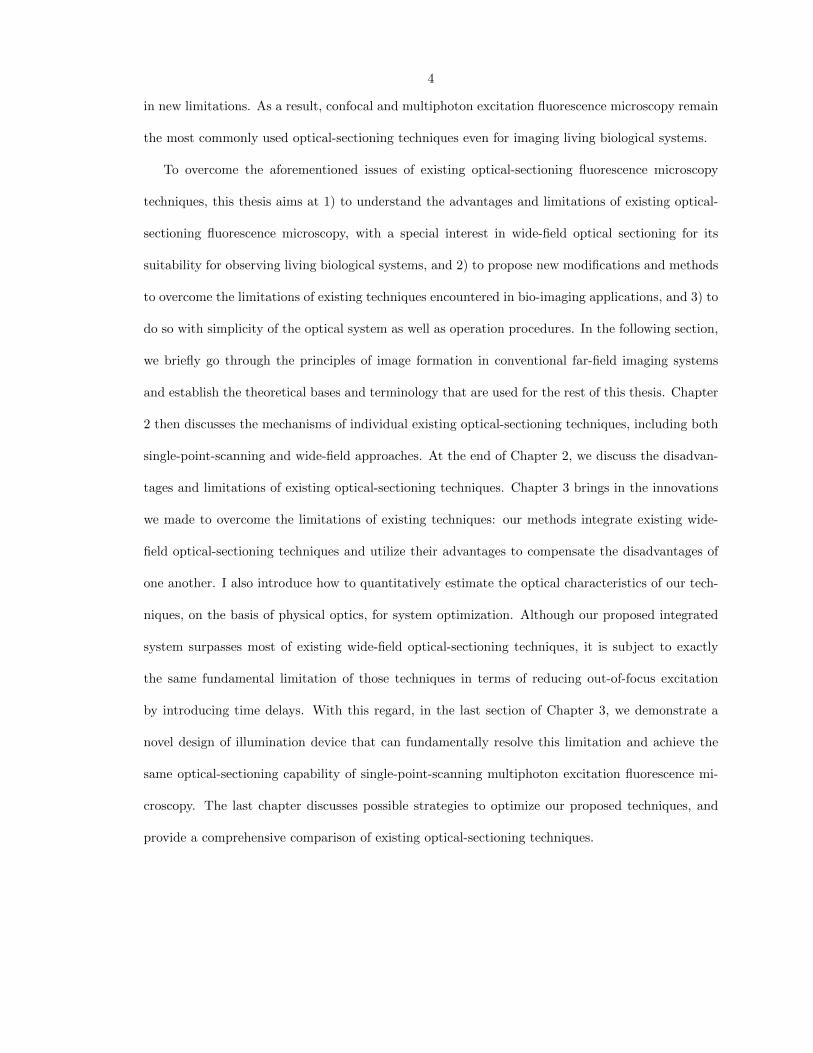
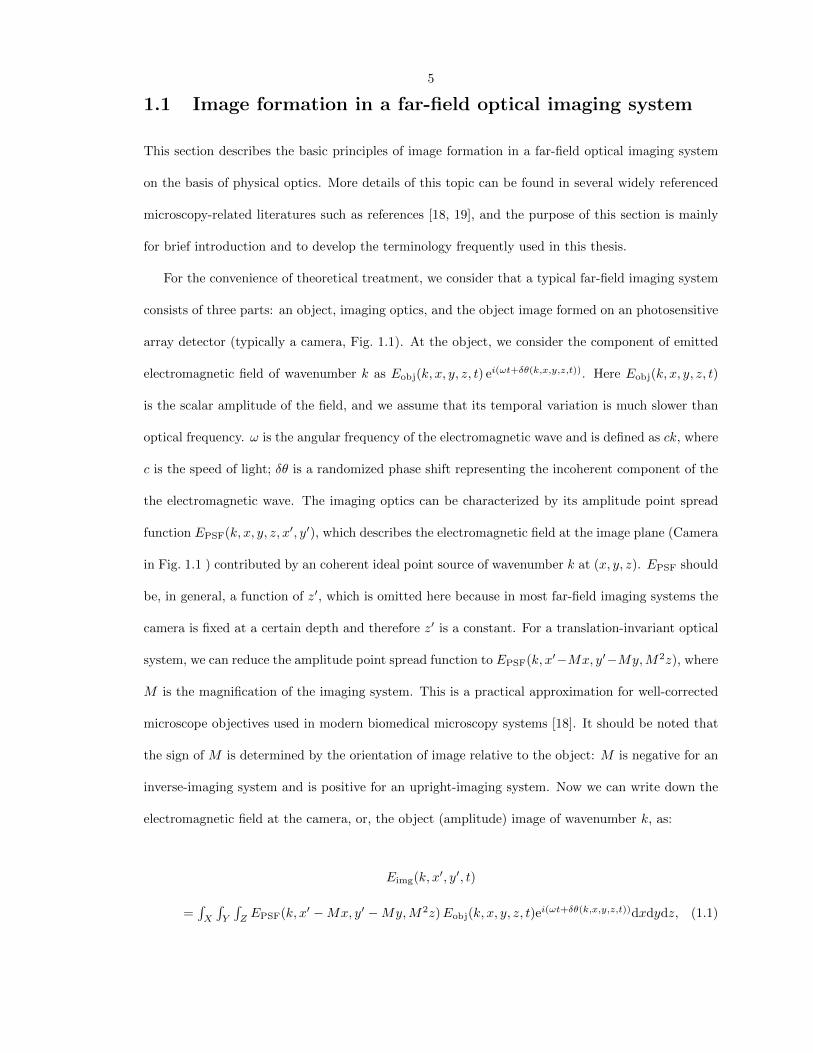
For the convenience of theoretical treatment, we consider that a typical far-field imaging system

consists of three parts: an object, imaging optics, and the object image formed on an photosensitive

array detector (typically a camera, Fig. 1.1). At the object, we consider the component of emitted

electromagnetic field of wavenumber k as Eobj(k, x, y, z, t) ei(ωt+δθ(k,x,y,z,t)). Here Eobj(k, x, y, z, t)

is the scalar amplitude of the field, and we assume that its temporal variation is much slower than

optical frequency. ω is the angular frequency of the electromagnetic wave and is defined as ck, where

c is the speed of light; δθ is a randomized phase shift representing the incoherent component of the

the electromagnetic wave. The imaging optics can be characterized by its amplitude point spread

function EPSF(k, x, y, z, x′, y′), which describes the electromagnetic field at the image plane (Camera

in Fig. 1.1 ) contributed by an coherent ideal point source of wavenumber k at (x, y, z). EPSF should

be, in general, a function of z′, which is omitted here because in most far-field imaging systems the

camera is fixed at a certain depth and therefore z′ is a constant. For a translation-invariant optical

system, we can reduce the amplitude point spread function to EPSF(k, x′−Mx, y′−My,M2z), where

M is the magnification of the imaging system. This is a practical approximation for well-corrected

microscope objectives used in modern biomedical microscopy systems [18]. It should be noted that

the sign of M is determined by the orientation of image relative to the object: M is negative for an

inverse-imaging system and is positive for an upright-imaging system. Now we can write down the

electromagnetic field at the camera, or, the object (amplitude) image of wavenumber k, as:

Eimg(k, x′, y′, t)

=∫X

∫Y

∫ZEPSF(k, x′ −Mx, y′ −My,M2z)Eobj(k, x, y, z, t)e

i(ωt+δθ(k,x,y,z,t))dxdydz, (1.1)

6

(x, y, z)

X

Y

Z

Imaging Optics

(x’, y’)

Camera

Object

(0, 0, 0)

Figure 1.1: Scheme of a typical far-field imaging system

or simply:

Eimg = EPSF ⊗X,Y,Z Eobj, (1.2)

indicating that the field profile at the image plane is a three-dimensional convolution (in X, Y , Z)

of the amplitude object and the amplitude point spread function of the imaging system [18, 19].

The camera, or the array detector, detects the intensity distribution, i.e., |E2img|, at the image

plane. The signal collected by a unit detector, commonly referred to as a ’pixel,’ is the integral of

intensity over the pixel area and exposure time [18, 19]; ’photon counts’ is commonly used as the

unit of such signals. For simplicity, we can consider that the camera is an array of infinitesimal

pixels, which allows us to omit the spatial integrations, and the signal per unit area collected by a

pixel at (x′, y′) at time t1 within an exposure time δt can be written as:

Iimg(k, x′, y′, t1, δt) =∫ t1+δt

t1|Eimg(k, x′, y′, t)|2dt

=∫ t1+δt

t1Eimg(k, x′, y′, t) · E∗img(k, x′, y′, t)dt

=∫ t1+δt

t1

∫Xa,Ya,Za,Xb,Yb,Zb

EPSF(k, x′ −Mxa, y′ −Mya,M

2za)E∗PSF(k, x′ −Mxb, y′ −Myb,M

2zb)

×Eobj(k, xa, ya, za, t)E∗obj(k, xb, yb, zb, t)

×ei(δθ(k,xa,ya,za,t)−δθ(k,xb,yb,zb,t))dxadyadzadxbdybdzbdt. (1.3)

7

Now if we assume that 1) the variation of Eobj in time is slow enough to be negligible during a δt

period, and 2) the electromagnetic field emitted at the object is spatially incoherent because the

coherent length is much smaller than the finest feature that can be resolved by the imaging system,

which is generally applicable to fluorescence imaging, we have:

∫ t1+δt

t1Eobj(k, xa, ya, za, t)E

∗obj(k, xb, yb, zb, t)e

i(δθ(k,xa,ya,za,t)−δθ(k,xb,yb,zb,t))dt

≈ δtEobj(k, xa, ya, za, t1)E∗obj(k, xb, yb, zb, t1) δ(x1 − x2, y1 − y2, z1 − z2). (1.4)

Combining eqs. 1.3 and 1.4 we derive:

Iimg(k, x′, y′, t1, δt)

≈ δt∫Xa,Ya,Za,Xb,Yb,Zb

EPSF(k, x′ −Mxa, y′ −Mya,M

2za)E∗PSF(k, x′ −Mxb, y′ −Myb,M

2zb)

×Eobj(k, xa, ya, za, t1)E∗obj(k, xb, yb, zb, t1) δ(xa − xb, ya − yb, za − zb)dxadyadzadxbdybdzb

= δt∫X,Y,Z

|EPSF(k, x′ −Mx, y′ −My,M2z)|2 |Eobj(k, x, y, z, t1)|2dxdydz

= δt∫X,Y,Z

IPSF(k, x′ −Mx, y′ −My,M2z) Iobj(k, x, y, z, t1)dxdydz

= δt IPSF ⊗X,Y,Z Iobj, (1.5)

where IPSF and Iobj respectively denote the intensity point spread function of the imaging optics and

the intensity profile of the object. Equation 1.5 shows us that when the electromagnetic field emitted

at the object is spatially incoherent, the image acquired by the camera is simply the convolution of

the intensity profile at the object and the intensity point spread function of imaging optics.

An important message we learn from eqs. 1.3 and 1.5 is that the 2-dimensional information

provided by the acquired image is actually a mixture of 3-dimensional information about the object,

which is now expressed explicitly as the 3-dimensional (X,Y, Z) convolution. Considering such a

dimension mixing and reduction process of image formation in an far-field imaging system, we can

realize that the acquired images does not provide reliable quantitative information about the object

even at the spatial resolutions of the imaging system. We can use a simple object, a constantly

8

bright point source at (0, 0, z0), to visualize such an issue. To calculate the image of this object, we

simply substitute δ(x, y, z − z0) for Iobj in eq. 1.5 so that:

Iimg(k, x′, y′) =

∫X,Y,Z

IPSF(k, x′ −Mx, y′ −My,M2z) δ(x, y, z − z0)dxdydz

= IPSF(k, x′, y′,M2z0). (1.6)

Here we can omit time-related terms as long as the point source is assumed to have a constant

brightness. To simplify the math, we assume the point spread function is in the form of a 00-mode

Gaussian beam so that:

Iimg(k, x′, y′) = I0

(w0

w(M2z0)

)2

exp

(−2 (x′2 + y′2)

w(M2z0)2

), (1.7)

where:

w(z) = w0

√1 +

zλ

πw20

. (1.8)

Equation 1.7 suggests that the image of a point source is a 2-dimensional Gaussian distribution

wherein the width of the distribution is a function of z0. A feature of conventional far-field imaging

revealed by eq. 1.7 is that the total signal collected by the array detector is more or less the same

no matter what the depth of the point source is. We can verify this feature simply by integrating

Iimg over x′ and y′:

∫ ∞−∞

∫ ∞−∞

Iimgdx′dy′

= I0

(w0

w(M2z0)

)∫ ∞−∞

∫ ∞−∞

exp

(−2 (x′2 + y′2)

w(M2z0)2

)2

dx′dy′

= I0

(w0

w(M2z0)

)2

× π w(M2z0)2

2= πI0 w

20/2, (1.9)

and the result shows no dependence on z0. Such a feature indicates that, when imaging a thick

sample, the signals coming from different depths, in terms of photon counts, have nearly equal

contributions to the acquired image. Noteworthily, the integral of signals obtained by the detector

9

as a function of the depth of a point source, as exemplified by eq. 1.9, is commonly referred to as

axial response. Axial response is frequently used to quantify the capability of optical sectioning of

an optical imaging system, and its full width at half maximum (FWHM) is typically defined as the

axial resolution of an optical-sectioning imaging system.

Theoretically it is possible to deconvolve a stack of images acquired at sequential depths with

the intensity point spread function to retrieve accurate spatial information about the object. Such

a method, however, is limitedly applied to biologically relevant imaging tasks because the fidelity

of the results of deconvolution demands sparsity of light-emitting sources in the object and high

signal-to-noise ratios of acquired images, which are not always satisfied in biological imaging and

especially not so when high-frame-rate imaging of fluorescent proteins is required.

Optical sectioning, on the other hand, takes a totally different approach to retrieve 3-dimensional

spatial information about the object. The main concept of optical sectioning is to manipulate the

axial response of an optical imaging system such that the maximal response occurs at the depth where

the IPSF has the narrowest lateral distribution. In certain types of optical-sectioning techniques the

signal coming from outside of half maximums of axial response can be considered negligible, which

makes the obtained spatial information accurate as long as the required axial and lateral resolutions

are not finer than the full widths at half maximums of axial response and lateral point spread

function of the imaging system. In the next chapter we discuss several optical-sectioning techniques

and their optical properties.

10

Chapter 2

Optical sectioning

2.1 Single-point-scanning optical sectioning: confocal and

multiphoton excitation fluorescence microscopy

2.1.1 Mechanism

Conventional confocal fluorescence microscopy and multiphoton excitation fluorescence microscopy,

although share similar optical designs and instrumentations [1, 2], achieve optical sectioning through

completely different mechanisms. Confocal fluorescence microscopy tightly focuses a beam onto the

object, and positions a pinhole or a small aperture at the conjugate point of the focal spot in

front of a photodetector [1, 20]. With such a geometrical arrangement, the pinhole allows most of

focal-spot emission going through while blocking most of emission outside of the focal spot, and

thus achieve optical sectioning. The axial response at out-of-focus region can be straightforwardly

derived as 1/z2 on the basis of geometrical optics. Rigorous derivations of the axial response of

confocal fluorescence microscopy, which convolves the focused beam profile with a modified IPSF

containing a pupil function to describe the pinhole, can be found in reference [20].

Multiphoton excitation fluorescence microscopy, on the other hand, utilizes the nonlinear excita-

tion efficiency to create optical sectioning [2]. For simplicity, we can again assume the focused beam

11

profile to be a 00-mode Gaussian beam, and, for 2-photon excitation, the axial response is:

∫X,Y

(I0

(w0

w(z)

)2

exp

(−2(x2 + y2)

w(z)2

))2

dxdy ∝ 1

w(z)2. (2.1)

From eq. 1.8 we can see that the axial response of two-photon excitation fluorescence microscopy is

approximately proportional to 1/z2 at out-of-focus regions. Alternatively, one can derive this 1/z2

out-of-focus response on the basis of geometrical optics, just as in the case of confocal fluorescence

microscopy.

2.1.2 Discussions

The 1/z2 axial response at out-of-focus regions in confocal and two-photon excitation fluorescence

microscopy is now the gold standard of optical-sectioning techniques. Nonetheless, the single-point-

scanning mechanism of these two techniques raises certain issues and limitations in bio-imaging

applications. Unlike conventional far-field optical image formation, the pixel-by-pixel signal acquisi-

tion of single-point-scanning mechanism drastically slows down the imaging speeds and complicates

the instrumentations. Meanwhile, to obtain images at reasonable frame rates, the dwell time of the

focal point at each pixel has to be short enough (typically from sub-µs to 100 µs), and thus requires

high focal intensity (typically > 105 times higher than in conventional wide-field fluorescence mi-

croscopy) for sufficient fluorescence emission. Such high focal intensity, however, has been found to

result in various photo-damages in living biological systems. Indeed, photo-toxicity in the scanned

live organisms has been frequently observed during video-rate time-lapse imaging on conventional

confocal microscopes [1]. Although such photo-toxicity can be greatly reduced by using multi-photon

excitation fluorescence microscopy [16, 21], a tradeoff is the thermal mechanical damage to living

tissues through the single-photon absorption of its near-infrared excitation [17].

An alternative approach to resolve photo/thermal-damages in conventional single-point-scanning

optical-sectioning microscopies without significant losses of acquisition speed is to implement the

capability of optical sectioning in wide-field optical microscopy. The wide-field microscopy techniques

12

mentioned here and hereafter in this thesis refer to those techniques wherein the image formation is

accomplished mainly by optical far-field imaging, and does not require a priori knowledge of spatial-

temporal information of illumination. In the next section we discuss several existing methods for

wide-field optical-sectioning microscopy including multifocal multiphoton microscopy, structured

illumination microscopy, temporal focusing, and selective plane illumination microscopy [7, 3, 5, 22,

6].

2.2 Existing methods for wide-field optical sectioning

2.2.1 Multifocal confocal microscopy and (time-multiplexed) multifocal

multiphoton microscopy

The concept of multifocal confocal microscopy and multifocal multiphoton microscopy is to have

multiple channels that excite and detect the fluorescence signal coming from the object in a tempo-

rally parallel manner [23, 4], so as to speed up the image formation process. In these techniques,

multiple foci are created as independent channels for excitation in and detection from the sample.

To preserve the capability of optical sectioning, however, the spatial distribution of foci has to

be sufficiently sparse, which limits the degree of parallelization. This is because signal crosstalk

among parallel channels in multifocal confocal microscopy and out-of-focus excitation in multifocal

multiphoton microscopy become significant as the interfocal distances of the foci decrease. Take an

oil-immersion NA 1.42 objective lens for example, the distance between neighboring foci dfoci that

preserves the 1/z2 axial response at out-of-focus regions is approximately 5 times of the excitation

wavelength λ [5], while the diameter of the focal spots f0 is approximately 0.3 λ, which makes the

fraction of un-illuminated area approximately 1 − (dfocid0)2 ≈ 99.6%. Such a high fraction of un-

illuminated area requires a large number of scanning steps to illuminate the entire field of view, and

thus greatly limit the improvements of imaging speed in multifocal confocal/multiphoton microscopy.

To cover the un-illuminated area, Egner et al. [5] proposed to use time multiplexing, i.e., gen-

erating multiple foci that are largely separated in time, so that the interferences among these foci

13

is negligible even though they partially overlap in space. The number of distinct time-delay steps

required to cover the un-illuminated area, Nt, can be estimated as

Nt ≈ (d0

dfoci)2 ≈ 280. (2.2)

Nonetheless, due to the difficulties of fabricating the temporal delay mask, an optical element that has

large numbers of distinct height levels on its surface, the number of distinct time delays practically

achieved to date through this approach is only 3. We further discuss the details about the fabrication

of temporal delay masks in Section 3.2 and 3.3.

2.2.2 Structured illumination microscopy

In contrast to multifocal confocal/multiphoton microscopy, structured illumination is a much more

successful example of achieving wide-field optical sectioning in terms of system complexity and imag-

ing speeds. The working principle of structured illumination microscopy is a fundamental property of

incoherent far-field imaging: higher spatial frequency components of the images decay more rapidly

with defocusing. Structured illumination microscopy illuminates the object with a high-spatial-

frequency excitation pattern and acquires several images with the excitation pattern translated

to different positions. Then a simple algorithm that filters high-spatial-frequency components is

applied to extract the in-focus fluorescence signal. Reference [3] shows, theoretically and experi-

mentally, that structured illumination microscopy shares a similar axial response as conventional

confocal microscopy.

However, the single-photon excitation of conventional structured illumination microscopy excites

the full depth of the sample within the field of view - an extremely inefficient use of the quantum yield

of the fluorophores that can lead to significant photobleaching in a thick object as found in confocal

microscopy. Also, at each acquisition, structured illumination microscopy receives fluorescence over

a full depth range and numerically removes most of it afterward. Such a procedure can sacrifice

the dynamic range of the camera for unwanted (out-of-focus) information and result in degraded

14

signal-to-noise ratios of the processed images.

2.2.3 Temporal focusing

Temporal focusing is a multiphoton excitation-based technique that inherits the concept of time-

multiplexed multifocal multiphoton microscopy: introducing time delays to reduce out-of-focus exci-

tation [6]. In temporal focusing, a light-scattering plate creates continuous time delays (in contrast

to multiple discrete time delays in time-multiplexed multifocal multiphoton microscopy). Instead

of forming a group of temporally separated foci, the net effect of such continuous time delays is

that the effective pulse duration of the excitation light pulses varies as the pulse propagates along

the optical axis, and is shortest at the conjugate plane of the light-scattering plate. Owing to the

nonlinear excitation efficiency of multiphoton excitation, the higher peak intensity associates with a

shorter pulse duration, which provides the optical-sectioning effect. Temporal focusing microscopy

was first experimentally demonstrated by Oron et al. [6]. In their setup, the laser pulse is directed to

a blazed grating, which serves as the light-scattering plate, in an oblique incidence orientation. The

illustration of the time course of temporal focusing resembles conventional multiphoton line-scan

mechanism. A geometry-based model can be used to estimate the effective pulse duration and as a

function of depth [6] and hence the optical-sectioning effect.

However, this implementation of temporal focusing relies on high-order diffracted beams for

excitation, and therefore the optical path of the system depends on the wavelength of the excitation

light. If one uses an ultrafast oscillator with a wavelength-tunable output as the excitation light

source, it is technically possible to build a mechanical arm system that can rotate and translate a

mirror to suit various wavelengths, but such an optical design is not practically favorable, and it does

not work for multiple excitations at the same time. As a result, temporal focusing is inconvenient

when multiple excitation wavelengths are required for imaging, which is frequently encountered in

bio-imaging tasks such as investigating the spatial-temporal correlations of two or more bio-molecules

in the specimen.

15

2.2.4 Selective plane illumination microscopy (SPIM)

Unlike most of the aforementioned techniques that use a single microscope objective for both illu-

mination and detection, selective plane illumination microscopy requires an additional illumination

path orthogonal to the detection path to deliver a sheet-like excitation profile [7, 24]. Recently, this

technique has been found particularly useful to observe cell motions during embryonic development

[7, 25].

However, the illumination mechanism of SPIM leads to a tradeoff between the size of the field of

view and axial resolution. This tradeoff results from the nature of diffraction of light: the smaller

the focal spot (or beam waist), the faster the beam converges and diverges, and thus the shorter

depth of focus. For example, if a 1-µm axial resolution is required, the width of field of view, i.e.,

the depth of focus of the illumination beam, would be no larger than 10 µm [26]. In addition, the

close proximity of separate illumination and imaging optics in SPIM raises the system complexity

considerably and can lead to sample-handling difficulties.

2.2.5 Brief summary

In summary, currently existing wide-field optical-sectioning techniques still have their own issues

in bio-imaging applications. These techniques may be useful for certain imaging tasks, but for

general bio-imaging purposes, single-point-scanning confocal and multiphoton excitation fluorescence

microscopy remains the most commonly used optical-sectioning methods, and this is true even for

imaging living biological systems. In this regard, the next chapter discusses the innovations we

made based on integrating existing techniques to compensate the drawbacks of one another; we

demonstrate that our proposed wide-field optical-sectioning imaging technique have a simple optical

design with optical performance equivalent to or better than single-point-scanning optical sectioning

techniques.

16

Chapter 3

New methods for wide-field opticalsectioning microscopy

3.1 Diffuser-based temporal focusing microscopy: generat-

ing temporal focusing without high-order diffraction

In this section I would like to present a simple approach by which we resolved the limitations

associated with single excitation wavelength and low acquisition rates in the original temporal-

focusing microscopes. As discussed previously, the optical path of conventional temporal-focusing

microscopy is wavelength-dependent because the diffraction angle of a high-order diffracted beam

depends on the central wavelength of the excitation light. One way to overcome this limitation is

to use a ground-glass diffuser rather than a blazed grating as the scattering plate, or, in terms of

diffraction, to use 0th-order diffracted beams rather than high-order diffracted beams. An illustration

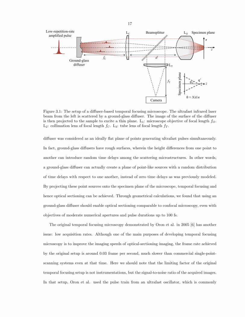
of such an optical system can be found in Fig. 3.1. The scattering pattern of a ground-glass diffuser is

dominated by zero-order diffraction, and thus the optical path is insensitive to the central wavelength

of the excitation light. The original report of temporal focusing by Oron et al., however, suggests that

using ground-glass diffusers to create sufficient temporal-focusing effect requires the pulse durations

of the laser to be shorter than 10 fs, even with high numerical-aperture (NA) objectives [6]. This

would make diffuser-based temporal focusing almost impractical, given the current pulse durations of

most commercially available light sources (∼100 fs). In their estimations, though, the ground-glass

17

Specimen plane LO LC

Ground-glass

diffuser

Low-repetition-rate

amplified pulse

LT

Beamsplitter

z

Camera

fC

fT

d

r

Spec

imen

pla

ne

q’ z θ

θ ≈ NA/n

Figure 3.1: The setup of a diffuser-based temporal focusing microscope. The ultrafast infrared laserbeam from the left is scattered by a ground-glass diffuser. The image of the surface of the diffuseris then projected to the sample to excite a thin plane. L1: microscope objective of focal length fO.L2: collimation lens of focal length fC . L3: tube lens of focal length fT .

diffuser was considered as an ideally flat plane of points generating ultrafast pulses simultaneously.

In fact, ground-glass diffusers have rough surfaces, wherein the height differences from one point to

another can introduce random time delays among the scattering microstructures. In other words,

a ground-glass diffuser can actually create a plane of point-like sources with a random distribution

of time delays with respect to one another, instead of zero time delays as was previously modeled.

By projecting these point sources onto the specimen plane of the microscope, temporal focusing and

hence optical sectioning can be achieved. Through geometrical calculations, we found that using an

ground-glass diffuser should enable optical sectioning comparable to confocal microscopy, even with

objectives of moderate numerical apertures and pulse durations up to 100 fs.

The original temporal focusing microscopy demonstrated by Oron et al. in 2005 [6] has another

issue: low acquisition rates. Although one of the main purposes of developing temporal focusing

microscopy is to improve the imaging speeds of optical-sectioning imaging, the frame rate achieved

by the original setup is around 0.03 frame per second, much slower than commercial single-point-

scanning systems even at that time. Here we should note that the limiting factor of the original

temporal focusing setup is not instrumentations, but the signal-to-noise ratio of the acquired images.

In that setup, Oron et al. used the pulse train from an ultrafast oscillator, which is commonly

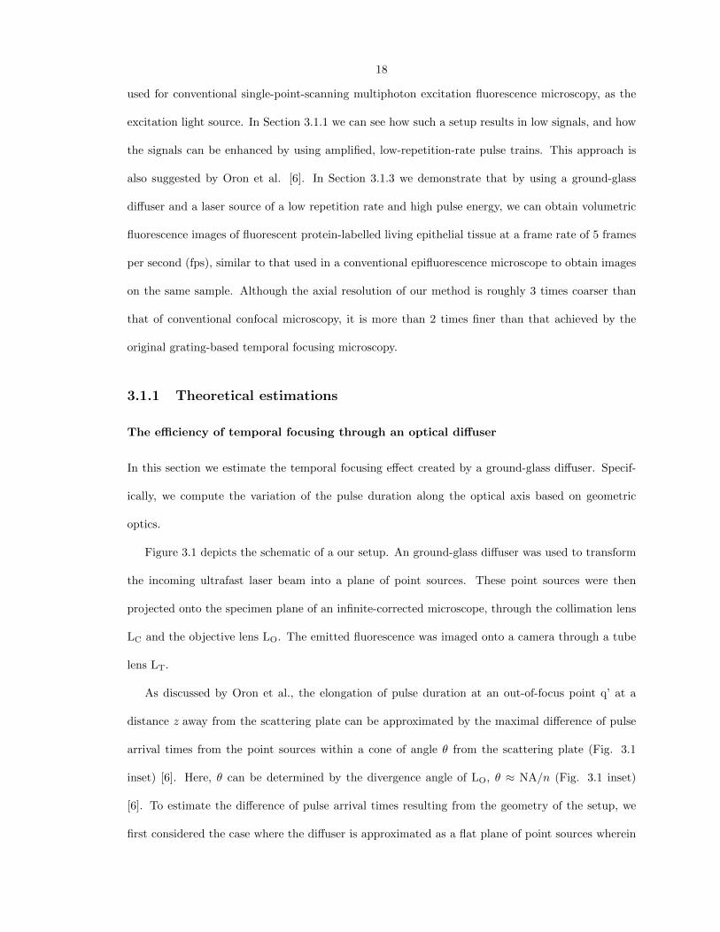
18

used for conventional single-point-scanning multiphoton excitation fluorescence microscopy, as the

excitation light source. In Section 3.1.1 we can see how such a setup results in low signals, and how

the signals can be enhanced by using amplified, low-repetition-rate pulse trains. This approach is

also suggested by Oron et al. [6]. In Section 3.1.3 we demonstrate that by using a ground-glass

diffuser and a laser source of a low repetition rate and high pulse energy, we can obtain volumetric

fluorescence images of fluorescent protein-labelled living epithelial tissue at a frame rate of 5 frames

per second (fps), similar to that used in a conventional epifluorescence microscope to obtain images

on the same sample. Although the axial resolution of our method is roughly 3 times coarser than

that of conventional confocal microscopy, it is more than 2 times finer than that achieved by the

original grating-based temporal focusing microscopy.

3.1.1 Theoretical estimations

The efficiency of temporal focusing through an optical diffuser

In this section we estimate the temporal focusing effect created by a ground-glass diffuser. Specif-

ically, we compute the variation of the pulse duration along the optical axis based on geometric

optics.

Figure 3.1 depicts the schematic of a our setup. An ground-glass diffuser was used to transform

the incoming ultrafast laser beam into a plane of point sources. These point sources were then

projected onto the specimen plane of an infinite-corrected microscope, through the collimation lens

LC and the objective lens LO. The emitted fluorescence was imaged onto a camera through a tube

lens LT.

As discussed by Oron et al., the elongation of pulse duration at an out-of-focus point q’ at a

distance z away from the scattering plate can be approximated by the maximal difference of pulse

arrival times from the point sources within a cone of angle θ from the scattering plate (Fig. 3.1

inset) [6]. Here, θ can be determined by the divergence angle of LO, θ ≈ NA/n (Fig. 3.1 inset)

[6]. To estimate the difference of pulse arrival times resulting from the geometry of the setup, we

first considered the case where the diffuser is approximated as a flat plane of point sources wherein

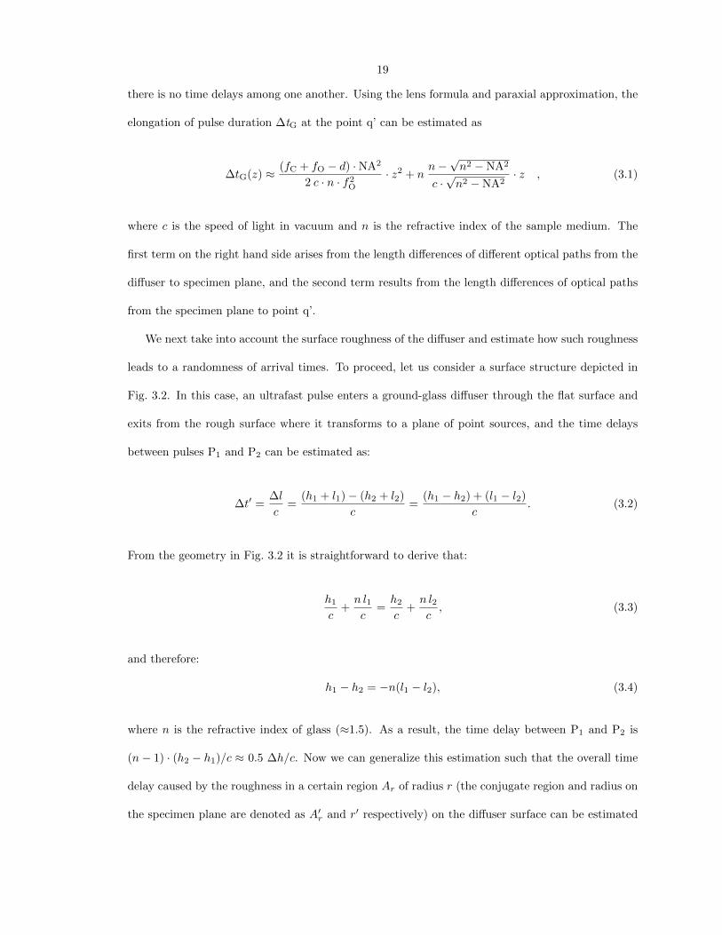
19

there is no time delays among one another. Using the lens formula and paraxial approximation, the

elongation of pulse duration ∆tG at the point q’ can be estimated as

∆tG(z) ≈ (fC + fO − d) ·NA2

2 c · n · f2O

· z2 + nn−√n2 −NA2

c ·√n2 −NA2

· z , (3.1)

where c is the speed of light in vacuum and n is the refractive index of the sample medium. The

first term on the right hand side arises from the length differences of different optical paths from the

diffuser to specimen plane, and the second term results from the length differences of optical paths

from the specimen plane to point q’.

We next take into account the surface roughness of the diffuser and estimate how such roughness

leads to a randomness of arrival times. To proceed, let us consider a surface structure depicted in

Fig. 3.2. In this case, an ultrafast pulse enters a ground-glass diffuser through the flat surface and

exits from the rough surface where it transforms to a plane of point sources, and the time delays

between pulses P1 and P2 can be estimated as:

∆t′ =∆l

c=

(h1 + l1)− (h2 + l2)

c=

(h1 − h2) + (l1 − l2)

c. (3.2)

From the geometry in Fig. 3.2 it is straightforward to derive that:

h1

c+n l1c

=h2

c+n l2c, (3.3)

and therefore:

h1 − h2 = −n(l1 − l2), (3.4)

where n is the refractive index of glass (≈1.5). As a result, the time delay between P1 and P2 is

(n− 1) · (h2 − h1)/c ≈ 0.5 ∆h/c. Now we can generalize this estimation such that the overall time

delay caused by the roughness in a certain region Ar of radius r (the conjugate region and radius on

the specimen plane are denoted as A′r and r′ respectively) on the diffuser surface can be estimated

20

Gla

ss

Air

h1

h2

l1

l2

∆l

P1

P2

Figure 3.2: Illustration of time delays generated by the surface roughness of a ground-glass diffuser.

as:

∆t′ ≈ 0.5∆h

c, (3.5)

where ∆h is the maximal surface height discrepancy within Ar.

As its name suggests, the roughness of an ground-glass diffuser is made by grinding a glass surface

with particles of sizes less than a certain length D. Thus, we expect ∆h → 0 when r → 0, and

∆h ≈ D if r � D, as shown in Fig. 3.3. To take into account these asymptotic estimations, we used

a simple approximation here: ∆h ≈ α · 2r if α · 2r < D and ∆h ≈ D if α · 2r ≥ D, where α is a

dimensionless roughness parameter of a ground-glass diffuser. Using this approximation, we obtain

a simple estimation of the difference of arrival times ∆t′ within Ar′ ,

∆t′ =

α fCc·fO · r

′ if α fCfO· r′ < 0.5D

0.5Dc if fC

fO· r′ ≥ 0.5D

=1

c·Min

[α fC

fOr′, 0.5D

]. (3.6)

For the out-of-focus point q’ shown in Fig. 3.1 (inset), Ar′ corresponds to the area covered by the

cone angle θ, and so we have r′ ≈ z · θ ≈ NAn z and

∆t′(z) =1

c·Min

[α fC

fO· NA

n· z , 0.5D

](3.7)

21

D

r ≈ 0

r >> D

Figure 3.3: Illustration of surface roughness of a ground-glass diffuser. Let ∆h denote the maximalsurface height discrepancy (i.e., the peak-to-valley difference) within an area of radius r (the con-jugate radius r′ on the specimen plane is of radius r fO/fD), we have ∆h → 0 when r → 0, and∆h ≈ D when r � D.

Combining eqs. 3.1 and 3.7, we finally obtain the effective pulse duration at an out-of-focus point q’

at distance z from the specimen plane, namely

τeff(z) = τ0 + ∆t′ + ∆tG (3.8)

= τ0 +Min

[α fCfO

NAn z , 0.5D

]c

+(fC + fO − d)NA2

2 c n f2O

z2 + nn−

√n2 −NA2

c√n2 −NA2

z, (3.9)

where τ0 is the pulse width of the laser source.

Figure 3.4 shows the numerical results of τeff(z) for the cases of three different objective lenses

commonly used for biomedical microscopy. Consistent with the report of Oron et al. [6], we find

that the contribution of ∆tG to τeff(z) is negligible when z ≈ Rayleigh length zR. Nevertheless, in

this small z regime, ∆t′ in eq. 3.9 can lead to a significant elongation of pulse width. In particular,

for the small z regions where α fCfO· NAn · z < 0.5D, eq. 3.9 can be simplified as:

τeff ≈ τ0(1 +α fC

fO· NA

τ0 n cz) = τ0(1 +

α fC

fO· n λ

π τ0 cNAz), with z ≡ z

zR≈ π NA2

n2 λz. (3.10)

Here, z is defined in units of Rayleigh length in order to facilitate the comparison of our results with

22

0.25

0.5

0.75

1

1

2

3

4

-5 -2.5 0 2.5 5

No

rma

lize

d fl

uo

resce

nce

sig

na

l

τe

ff (τ

0)

Distance (zR)

10X NA 0.3

40X NA 0.45

60X NA 1.42

Figure 3.4: Effective pulse durations and two-photon excitation strengths as functions of z underdifferent objectives lenses. The numerical results were obtained from eq. 3.9. Notice that eq. 3.11predicts z∗ ≈ 3.53, 2.21, and 1.62 for these objectives lenses, respectively, which are comparable withthe numerical results. The inverse of τeff was used to represent S2p (see eq. 3.15). The horizontal(distance) and vertical (τeff) axes are expressed in units of Rayleigh length and τ0, respectively.Parameters: fC =180 mm, D = 100 µm, d = 200 mm, λ = 800 nm, and τ0 = 100 fs. Objective lens10X: NA=0.3, fO =18 mm, n = 1. Objective lens 40X: NA=0.75, fO =4.5 mm, n = 1. Objectivelens 60X: NA=1.1, fO =3 mm, n = 1.33 (water immersion).

conventional confocal and two-photon scanning microscopy. We further define

z∗ ≡ fO

fC· π τ0 cNA

n λ=

π τ0 c

λ α fC· fO NA

n, (3.11)

whereby at z = z∗, τeff ≈ 2τ0, i.e., z = zRz∗ indicates positions at which the effective pulse width is

doubled. For two-photon excitation, this corresponds to the positions where the fluorescence signal

drops to half of the maximum. In conventional confocal and two-photon scanning microscopy, the

corresponding z∗ is ∼ 1. From the calculations outlined in Fig. 3.4, we find that optical sectioning

is comparable with conventional confocal microscopy, with either moderate (0.3-0.75) or high (>1)

NA objectives. Moreover, we find that laser pulses of 100-fs durations are sufficient to provide such

sectioning effects.

23

The efficiency of multiphoton excitation at low repetition rate

To solve the limitation of low frame rate, we next examine how the repetition rates of pulsed lasers

influence the efficiency of two-photon excitation (at constant average power). In short, we find that

a 105-fold increase in signal-to-noise ratios is obtained by lowering the repetition rate from 100 MHz

to 1 kHz, thus providing a signal level comparable to that of conventional multiphoton excitation

fluorescence microscopy.

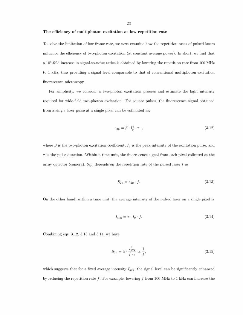
For simplicity, we consider a two-photon excitation process and estimate the light intensity

required for wide-field two-photon excitation. For square pulses, the fluorescence signal obtained

from a single laser pulse at a single pixel can be estimated as:

s2p = β · I2p · τ , (3.12)

where β is the two-photon excitation coefficient, Ip is the peak intensity of the excitation pulse, and

τ is the pulse duration. Within a time unit, the fluorescence signal from each pixel collected at the

array detector (camera), S2p, depends on the repetition rate of the pulsed laser f as

S2p = s2p · f. (3.13)

On the other hand, within a time unit, the average intensity of the pulsed laser on a single pixel is

Iavg = τ · Ip · f. (3.14)

Combining eqs. 3.12, 3.13 and 3.14, we have

S2p = β ·I2avg

f · τ∝ 1

f, (3.15)

which suggests that for a fixed average intensity Iavg, the signal level can be significantly enhanced

by reducing the repetition rate f . For example, lowering f from 100 MHz to 1 kHz can increase the

24

signal 105-fold without increasing the average light intensity delivered to the specimen. It should

be noted that the Ip of our low-repetition-rate setup is of similar order of magnitude as that used

in high-repetition-rate point-scanning microscopies. Thus, the signal levels of these two schemes are

predicted to be comparable.

3.1.2 Methods and Materials

The light sources we used in this work are ultrafast chirped pulse Ti:Sapphire amplifiers. Two

different models were used for the convenience of collaborations. Live-cell imaging was studied

(see Fig. 3.6) with a Spectra-Physics R© Spitfire R© Pro, seeded with a Spectra-Physics R© Mai Tai R©

SP ultrafast oscillator situated parallel to the amplifier within an enclosure. Measurement of axial

responses was carried out with a Coherent R© Legend Elite-USP-1k-HE, seeded with a Coherent R©

Mantis-5 ultrafast oscillator located parallel to the amplifier. The pulse durations, defined as the

FWHM of the temporal profiles of both amplifiers was approximately 35 fs or less. The wavelength

of both amplifiers was centered approximately at 800 nm with FWHM ≈30 nm. We expanded the

beam size by telescoping such that the beam profile on the diffuser was 2D Gaussian with FWHM ≈

20 mm. The maximal output of the laser amplifier was ∼3 Watt (average power), and was attenuated

to avoid thermal damage to biological specimens. The average laser powers reported in the following

sections were all measured at the back aperture of the objective lens LO.

The ground-glass diffuser employed was a Thor Labs model DG10-120. Diffusers, in general,

can cause significant inhomogeneities of the light intensity at the image plane. To reduce these

inhomogeneities, glass etching cream (Armour Etch R©) was used to etch the diffuser. The roughness

parameters D and α of the diffuser were found to be 30 µm and 0.1 after etching, according to the

surface profile we measured.

As shown in Fig. 3.1, the collimated laser beam is scattered by the ground-glass diffuser, col-

limated by the diffuser lens LC, and then projected to specimen plane via the objective lenses

(LUMFLN 60XW NA 1.1, PLANAPO N 60X NA 1.42). The LUMFLN model objective was used

for the living biological samples owing to its long working distance. The PLANAPO objective was

25

used for the quantitative characterizations and the fixed biological sample.

The chromatic dispersion of the full optical path was pre-compensated by the built-in compressor

of the ultrafast amplifiers such that the signal level at the specimen plane was maximized. Images

ware obtained by a CCD camera (iXon DU-885K, Andor) through LT. The field of view is a ∼6.4-

by-6.4 mm2/MO square, where MO is the nominal magnification of LO. The illumination field is 2D

Gaussian with FWHM ≈ 20 mm/MO. A larger illumination field or more uniform profile can be

obtained by further expanding the laser beam before the ground-glass diffuser.

The axial resolution was determined by taking images along the optical axis of a thin layer

(thickness less than 2 µm) of fluorescein (F-1300, Invitrogen). For living-cell imaging, we used

human mammary gland MCF-10A cells expressing cyan fluorescent protein-conjugated histone (H2B-

cerulean), which binds to chromosomes and has been widely used to indicate cell nuclei. MCF-10A

cells were seeded in 3-D matrigel (BD MatrigelTM) for 10 days to form bowl-shape cell clusters of

several hundred micrometers in size. We then used the cell clusters to evaluate the high-frame-rate

acquisition and optical sectioning capabilities of our diffuser-based temporal focusing microscope.

Following the acquisition of optical sections, three-dimensional views of the epithelial tissue were

reconstructed using 3-D Viewer of ImageJ.

3.1.3 Results

The axial resolution of diffuser-based temporal focusing microscopy is comparable to

conventional confocal microscopy

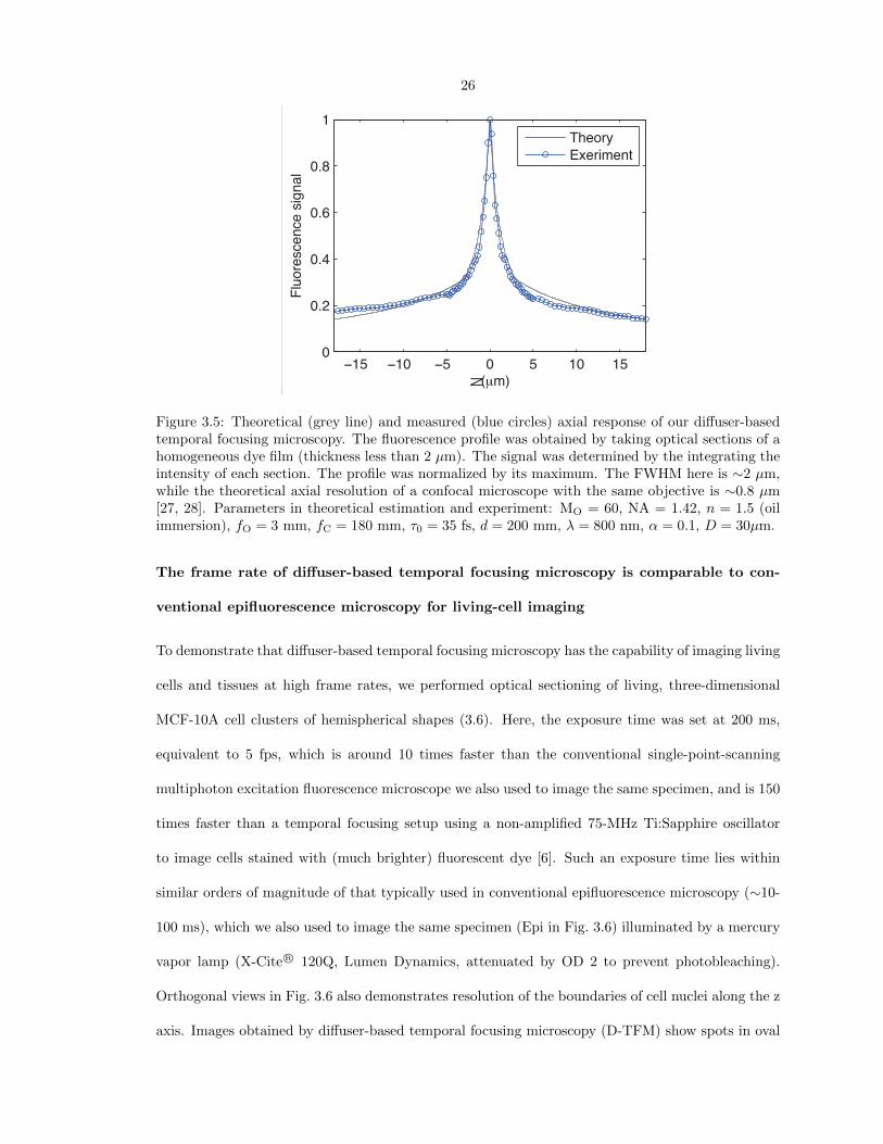
Figure 3.5 shows the axial resolution of the optical setup depicted in Fig. 3.1. Axial resolution was

determined by the FWHM of measured axial response. With MO = 60, NA ≈ 1.42, n ≈ 1.5, the

axial resolution was found to be ∼2 µm, and the corresponding z∗ ≈ 3. This is comparable to the

axial resolution of an optimized conventional confocal microscope, which has z∗ ≈ 1. Note that it

should be possible to obtain an axial resolution of z∗ ≈ 1 by optimizing the microscope design, as

we discuss in Section 3.1.4.

26

!" !# " # " !# !"#

#$%

#$&

#$'

#$(

!

)*+µ,-

./0123453653*47869/

*

*

:;312<

=>327,36?

Yu et al., J Biomed Opt, 16, 11, 2011

• 

• 

Figure 3.5: Theoretical (grey line) and measured (blue circles) axial response of our diffuser-basedtemporal focusing microscopy. The fluorescence profile was obtained by taking optical sections of ahomogeneous dye film (thickness less than 2 µm). The signal was determined by the integrating theintensity of each section. The profile was normalized by its maximum. The FWHM here is ∼2 µm,while the theoretical axial resolution of a confocal microscope with the same objective is ∼0.8 µm[27, 28]. Parameters in theoretical estimation and experiment: MO = 60, NA = 1.42, n = 1.5 (oilimmersion), fO = 3 mm, fC = 180 mm, τ0 = 35 fs, d = 200 mm, λ = 800 nm, α = 0.1, D = 30µm.

The frame rate of diffuser-based temporal focusing microscopy is comparable to con-

ventional epifluorescence microscopy for living-cell imaging

To demonstrate that diffuser-based temporal focusing microscopy has the capability of imaging living

cells and tissues at high frame rates, we performed optical sectioning of living, three-dimensional

MCF-10A cell clusters of hemispherical shapes (3.6). Here, the exposure time was set at 200 ms,

equivalent to 5 fps, which is around 10 times faster than the conventional single-point-scanning

multiphoton excitation fluorescence microscope we also used to image the same specimen, and is 150

times faster than a temporal focusing setup using a non-amplified 75-MHz Ti:Sapphire oscillator

to image cells stained with (much brighter) fluorescent dye [6]. Such an exposure time lies within

similar orders of magnitude of that typically used in conventional epifluorescence microscopy (∼10-

100 ms), which we also used to image the same specimen (Epi in Fig. 3.6) illuminated by a mercury

vapor lamp (X-Cite R© 120Q, Lumen Dynamics, attenuated by OD 2 to prevent photobleaching).

Orthogonal views in Fig. 3.6 also demonstrates resolution of the boundaries of cell nuclei along the z

axis. Images obtained by diffuser-based temporal focusing microscopy (D-TFM) show spots in oval

27

shapes, resembling the normal shape of cell nuclei. In contrast, the orthogonal view obtained by

epifluorescence microscopy shows distortion of the proper cell nuclear shape, due to the spreading

of the out-of-focus signal in an epifluorescence microscope. These results suggest that diffuser-based

temporal focusing microscopy can achieve high-frame-rate optical sectioning on living cells.

Inhomogeneity of the illumination field can be reduced by rotating the diffuser

In this study, we found that conventional diffusers can cause a significant inhomogeneity of the

light intensity in the illumination field, i.e., bright spots. The observed field inhomogeneity leads to

inhomogeneous sectioning capability across the field of view, the level of which can be measured by

imaging a homogenous dye film, then separating the field of view into several areas and comparing

the FWHMs of their axial responses. In our setup, the standard deviation of the FWHMs was found

to be ∼ 0.3µm. One way to reduce this inhomogeneity is through the use of multiple diffusers.

However, each diffuser would generate a certain level of time delay and thus contribute to pulse

broadening. As an alternative solution, we have chosen to simply rotate the diffuser. By rotating

the optical diffuser during the acquisition of a single frame, the inhomogeneities in the illumination

field are averaged out. This effect is demonstrated in Fig. 3.7.

3.1.4 Discussion

Optimization and limit of axial resolution

Equation 3.11 suggests that z∗ can be further reduced by using an objective with a higher magni-

fication and NA (which often exhibits a smaller fO NAn ), as shown in Fig. 3.4. Likewise, increasing

fC, α, or reducing τ0 leads to smaller z∗. We should note that these estimations are derived based

on geometrical optics, and are not valid when z∗ < 1, in which case the optimal axial resolution

of our temporal focusing setup would be the same as that of a single-point-scanning multiphoton

excitation fluorescence microscope [6].

A fundamental advantage of diffuser-based temporal focusing over grating-based approaches is

that the diffuser-based technique can achieve the axial resolution of a single-point-scanning setup,

28

10 µm

z = 0 µm z = 3 µm z = 6 µm

z = 9 µm z = 12 µm z = 15 µm

z = 18 µm z = 21 µm z = 24 µm

D-TFM

Epi

D-TFM

Epi

5 µm

Z

X

Figure 3.6: Optical sections and orthogonal views of living MCF-10A cells in a hemispherical struc-ture. The top panel shows the images obtained at sequential depths. The bottom panels showthe reconstructed orthogonal views under a diffuser-based temporal focusing microscope (D-TFM)and a conventional epifluorescence microscope (Epi), respectively. In the orthogonal view from theepifluorescence microscope, we clearly observe the residual out-of-focus light at the top and bottomedges of the nuclei. The blue lines indicate the positions where the orthogonal views were taken.Fluorescence signals were from cell nuclei expressing cyan fluorescent protein-conjugated histone(H2B-cerulean). Exposure time of each frame: 0.2 seconds. LO: 60X, NA ≈ 1.1, n ≈ 1.33. Stepsize: 1 µm. Laser average power: <10 mW.

29

STD/AVG ≈ 1 STD/AVG ≈ 0.3

Rotating diffuser Fixed diffuser

3 µm

Rotating diffuser can mitigate the inhomogeneity

Figure 3.7: Illumination field intensity inhomogeneity with fixed (left) and rotated (right) opticaldiffusers. The field inhomogeneity is defined as the standard deviation (STD) of the field dividedby the average (AVG) intensity of the field. The field inhomogeneity is greatly reduced by rotatingthe optical diffuser during the exposure of each frame. The sample is a homogeneous dye layer.

whereas (single) grating-based temporal focusing is limited to that of a line-scan setup. The dif-

ference arises from the way in which the time delays are generated. For ground-glass diffusers,

the time delay results from the surface roughness of the diffusers, which creates a two-dimensional

spatial profile for the randomness of the time delay. In contrast, the time delay in grating-based

temporal focusing is created by the one-dimensional scan of the laser pulses on the grating surface.

This restriction has been overcome by using two orthogonally aligned gratings [29]. In such a setup,

the two gratings must differ in groove density sufficiently, such that the scanning of the laser pulse

can be well separated in two orthogonal dimensions [29]. Such a design increases the complexity

of the apparatus and will likely require multiple pairs of gratings when multiple/tunable excitation

wavelengths are used.

From eq. 3.7, the spread, or distribution, of arrival times produced from the surface roughness of

a diffuser is upper bounded by the factor D. This suggests that diffusers with larger D should be used

to ensure a sufficiently large spread of arrival times. The roughness of the diffuser surface, however,

leads in turn to roughness of the image plane, D′. Using the thin lens formula, we estimate D′ to

be ( fOfC )2D. This suggests that D′ can be negligible if fC � fO. Thus, with a proper arrangement

of parameters, the roughness of the image plane can be reduced below one Rayleigh length, while

the surface roughness of the diffuser is sufficiently large to create temporal focusing.

30

Limitation of frame rate and benefits of low repetition rate

For living-tissue imaging, the frame rates of our setup are limited by the relatively low excitation

efficiency (compared with organic fluorescent dyes) of fluorescent proteins expressed in living systems.

Nevertheless, eq. 3.15 suggests that signal-to-noise ratios can be further enhanced by lowering the

repetition rate while maintaining the average power of the laser. For example, the frame rate of our

setup can be further increased by equipping our system with a pulsed laser of much lower repetition

rate, e.g., 100 Hz. With such a low repetition rate, eq. 3.15 suggests a 10-fold stronger signal-to-noise

ratio than what is presented in this study. This would lead to a frame rate of up to 50 fps, a rate

sufficient to study most biological processes such as cell division, migration, and polarity formation.

Here we estimate the limit of frame rates based on imaging the fluorescent proteins expressed in

living systems. This limitation is relaxed, though, if the signals are derived from materials with

strong fluorescence efficiency such as fluorescent dyes and nanoparticles.

Our setup can achieve the large field of view with a relatively short exposure duration simply

because the 1-kHz amplifier is very powerful; that is, because it is supplying its average power at a

low repetition rate and low duty cycle and thus achieving a high peak power. To generate multi-

photon excitation at the level required for imaging with reasonable frame rates, the peak intensity

is commonly around or greater than 1 kW/µm2 [2]. Therefore, to excite an area up to 1 mm2,

one needs a light source with peak power greater than 109 Watt. The maximal peak power of our

amplifier is roughly 1011 Watt, and is thus powerful enough to support a large field of view for

most microscopy applications. It should be noted that in the original temporal focusing setup [6], a

140-by-140-µm field of view was obtained with an average power of 30 mW and an exposure time

of 30 seconds. This indicates that a 1-mm2 field of view can be achieved with that instrument by

using a low magnification objective and an average power of around 1.5 Watt, though the exposure

time in such a setup could be slightly longer than 30 seconds because lower magnification objectives

are typically less efficient in collecting light.

However, from a biologist’s point of view, we would also like to point out that discussing the

imaging speed for fixed biological samples stained with fluorescent dye is less important than the

31

speed achievable for living systems. Once a sample is fixed, using an imaging time of either 3 hours

or 10 seconds would most likely provide the same level of details and information. On the other

hand, for the studies of dynamic biological process, the imaging speed would determine the temporal

resolution of the observations. To the best of our knowledge, this is the first report of imaging live

cells expressing fluorescent protein by a temporal focusing microscope at a frame rate faster than 1

fps.

In addition to the enhancement of the signal level and frame rate, there are certain potential

benefits provided by lowering the repetition rate from the MHz to kHz regime. It has been reported

that the use of low repetition rates (at the same optical power) can reduce photobleaching [30, 31].

This is achieved through the avoidance excitation during dark state conversion, which is believed

to be a photobleaching mechanism. Indeed, a 5- to 25-fold enhancement of total fluorescence yield,

before detrimental effects from photobleaching, has been experimentally measured [30]. Moreover,

lowering the repetition rate is equivalent to providing the system a longer window of no excitation.

This would allow slow processes such as heat dissipation to occur more efficiently, thus minimizing

sample damage caused by a continuous accumulation of heat. As a result, even with a similar amount

of thermal energy introduced by the excitation process, a sample excited at a low-repetition-rate

light pulses is less likely to be damaged by heat accumulation as compared to the use of a high-

repetition-rate light pulses [17].

Potential applications as structured illumination microscopy

In principle, the inhomogeneity of the illumination field can be utilized for structured illumination

microscopy [3]. This could be particularly useful in applications where reasonable optical section-

ing, as provided by temporal focusing, is not achievable. Examples include coherent anti-Stokes

Raman scattering (CARS) and stimulated Raman scattering microscopy, where picosecond pulses

are generally required to obtain chemical specificity [32, 33]. Based on Equation 3.11, ultrafast pulse

trains of picosecond duration would greatly reduce the sectioning effect. Nevertheless, by using the

inhomogeneity of the illumination field as a structured light source, it is possible to regain sectioning

32

capability of these systems, as demonstrated in a previous study [3]. This allows one to integrate

CARS with multiphoton excitation in a wide-field microscope simply by using a ground-glass diffuser.

3.1.5 Brief summary

The question of how to increase image acquisition rate and axial resolution, while maintaining a

bio-compatible laser dosage, is a long-standing challenge in the community of optical microscopy.

In this report, we have demonstrated a microscope design for living-tissue imaging that provides an

axial resolution comparable to confocal microscopy and a frame rate similar to that of epifluorescence

microscopy.

By utilizing an ground-glass diffuser, a temporal focusing setup is realized with a design as simple

as a conventional epifluorescence microscope. Even at a high frame rate, the photobleaching and

thermal damage of diffuser-based temporal focusing microscopy could be lower than single-point-

scanning multiphoton excitation fluorescence and confocal fluorescence microscopy. Compared with

temporal focusing techniques using MHz repetition-rate laser pulse trains, the use of low repetition-

rate pulses, while maintaining the same average power, can significantly enhance the signal-to-noise

ratio. In addition, using an ground-glass diffuser instead of a blazed diffraction grating provides

flexibility for multi- or tunable-wavelength light sources, and thus creates a platform for multi-

spectral imaging and pump-probe microscopy. Taken together, these features suggest that diffuser-

based temporal focusing microscopy can be used to study fast, three-dimensional processes in living

cells and tissues, and to do so with minimal photo-toxicity and thermal damage.

3.2 Temporal focusing or dense time multiplexing by height-

staggered microlens array

In previous sections we see how time delays and temporal focusing can be generated using 0th-order

diffracted beams rather than high-order diffracted ones so as to avoid wavelength dependent optical

paths. However, we see that the usage of ground-glass diffusers also introduce inhomogeneity of

33

Yu et al., Opt Express, 21, 2, 2013

Specimen plane L1 L2 HSMA Incoming pulse

L3

Beamsplitter

z

Camera

XY stage

f2

f3

f2

HSMA

Unit array of HSMA:

2-dimensional

arrangement of time

delays

Figure 3.8: Setup of a HSMA-based temporal focusing microscope. L1 is the microscope objectivelens. L2 and L3 are tube lenses of focal length fT . XY stage performs the lateral translations of themultifocal pattern. The specimen plane is defined as the focal plane of the objective lens L1. Insetsillustrate a spiral HSMA used in this study.

illumination field. Although shifting or rotating the diffuser during exposure can mitigate such

inhomogeneity, it can also decrease frame rates greatly. Other issues of diffuser-based temporal

focusing include moderate axial resolution and inefficient uses of the excitation light. All of these

drawbacks, interestingly, trace back to the random scattering structures of ground-glass diffusers.

To further improve the field homogeneity and axial resolution and to use excitation light ef-

ficiently, we proposed to use a new optical element that has engineered scattering structures for

generating temporal focusing: an array of microlenses with height differences among one another.

Figure 3.8 shows the schematic of such a microscope. This height-staggered microlens array (HSMA)

has a constant lens pitch across the entire array, so that field homogeneity can be achieved by sim-

ply shifting the array for a few steps. The focusing power of individual microlenses can be made to

match the back aperture of the objective lens so that each focus shows axial response similar to that

of a single-point-scanning multiphoton excitation fluorescence microscope near the focal plane of the

objective lens. At out-of-focus regions, the height staggering among the microlenses can introduce

time delays which leads to temporal focusing effect and thus reduces out-of-focus excitation.

In this section, we discuss how to implement such a concept and how to estimate its optical

34

performance; we also experimentally compare its axial response with that of a confocal microscope,

and demonstrate sectioning imaging on living C. elegans. We should note here that the combina-

tion of microlens arrays and temporal masks, as used in time-multiplexed multifocal multiphoton

microscopy (TM-MMM) [5], can provide equivalent functions of the proposed HSMAs, although

additional precision alignment and positioning are required.

Before diving into the details of our HSMA-based temporal focusing technique, it is worthwhile to

discuss the difference between our technique and TM-MMM. While both of these techniques reduce

out-of-focus excitation by introducing time delays among foci, the goals of system optimization are

different. In TM-MMM, an upper limit of out-of-focus excitation is set and the goal of optimization

is to arrange foci as (spatially) close to one another as possible until this limit is reached [5]. Because

in the original TM-MMM this limit is set almost as low as that in single-point-scanning multiphoton

microscopy, the result of such optimization, as we can see later, is that the foci are far apart from

one another and thus a large number of scanning steps (∼100 or larger) are required to illuminate

the entire field of view. Our approach, on the other hand, fixes the interfocal distances at around

twice of the diameter of a focal spot so that only ∼4-10 scanning steps are required to fulfill the

filed of view, and we try to minimize out-of-focus excitation by manipulating the distribution of

time delays among foci. The disadvantage of such an approach is that the out-of-focus excitation is

moderately suppressed, and to overcome this issue we utilized the multifocal pattern to implement

structured illumination microscopy [3] to remove out-of-focus signals from the acquired images.

3.2.1 Design of a HSMA-based temporal focusing microscope

We begin the design of HSMAs with the consideration of their physical limitations. The dimensions

of HSMAs are limited by fabrication technologies as well as diffractive losses. Existing techniques

cannot straightforwardly engineer micro-optics of depth variation >1 mm [34]. In addition, when

we consider the HSMA as an array of time-delay channels, a light pulse propagating in one channel

can leak into its neighboring channels due to the nature of diffraction. To quantify such an effect,

we use a simple model consisting of two adjacent microlenses with height staggering ∆h, as shown

35

in Fig. 3.9. When the light of wavelength λ0 exits from channel 1 (Ch1) and propagates to distance

z, diffraction theory predicts the beam size, dB, as a function of λ0 and z. With this regard, we

consider the inter-channel leakage to be non-negligible if dB before propagating to z = ∆h is larger

than the pitch of the microlens array, d. In other words, the inter-channel leakage is negligible if

dB ≤ d for z ≤ ∆h. (3.16)

A reasonable design, as shown in Fig. 3.9, is to set the focus of Ch1 at z = ∆h, so that dB decreases

upon exiting Ch1 and reaches its minimum, df , at z = ∆h. Based on the diffraction-limited spot

size of an ideal thin lens, we can estimate df as

df ≈ 1.22 λ0 × f#, (3.17)

where f# is defined as f/d [35]. Combining eqs. (3.16), (3.17) and the geometry, we have

d ≥ 1.22 λ0 ×f

d≈ λ0 ×

∆h

d, (3.18)

and the criterion of negligible inter-channel light leakage is thus

d ≥√λ0∆h. (3.19)

To ensure the inter-channel light leakage is negligible regardless of the geometrical arrangements of

distinct time-delay steps, we can substitute the largest height difference in the HSMA, ∆hmax, for

∆h in eq. (3.19), and thus derive

d ≥√λ0∆hmax. (3.20)

The argument here also applies to the design of the combination of temporal masks and microlens

arrays used in TM-MMM [5]. In such a case, the ends of the time-delay channels are flat surfaces,

and one can use the single-slit diffraction to approximate the beam size with propagation. Such an

36

∆h

f

df d Ch1

Ch2

z 0 *negligible inter-channel leakage: df ≤ d

Figure 3.9: A model of two adjacent microlenses. d: aperture of the microlenses. f : focal length ofthe microlens. df : the diameter of the focal spot. ∆h: height difference between two microlenses.

approach yields a similar criterion.

Accordingly, we restrict ∆hmax to ∼ 300 µm and 36 µm ≥ d ≥ 18 µm, via eq. (3.20). These

dimensions make the HSMA fabrication feasible through existing techniques, and can provide up to

∼ 106 foci within a 2-inch aperture. For a simple analysis, we assume that the total amount of time

delay ∆ttot is separated equally into Nt distinct time-delay steps (with step size ∆t, eq. (3.21)).

These time-delay steps are then arranged in a prescribed periodic pattern in the HSMA (Fig. 3.8

insets). Considering the propagation speed of light in a material as in the case of Fig. 3.2, we have:

∆ttot ≡ (Nt − 1)×∆t =∆hmax (n− 1)

c, (3.21)

where c and n are the speed of light in vacuum and the refractive index of the material of the HSMAs

(set to be 1.5), respectively.

Because of the limitation of ∆hmax, the estimated ∆t in eq. (3.21) can be around or shorter than

the pulse duration of conventional ultrafast oscillators or amplifiers above certain values of Nt. In

such cases, we should take into account the temporal interferences among light pulses of different

time delays. Notably, temporal masks with much larger ∆ttot have been proposed to avoid temporal

interferences and to achieve scanningless TM-MMM [5], and here we can estimate the size of such

HSMAs using the criterion derived previously.

As estimated in Section 2.2.1, the number of distinct time-delay steps Nt required to achieve

is ∼280. The appropriate values of ∆t for negligible temporal interferences, as suggested in the

previous study of TM-MMM [5], are equal to or larger than twice the pulse duration of the light

pulse, τ0, i.e., ∆t ≥ 2 τ0 (where τ0 was set as ≈ 100 fs for conventional ultrafast oscillators) [5].

37

Accordingly, we find that ∆hmax ≈ 33 mm and d ≈ 0.15 mm using eqs. (3.20)-(3.21), wherein λ and

n are assumed to be ∼ 800 nm and 1.5, respectively; such a ∆hmax falls far beyond the limits of

existing fabrication techniques. Further, if one needs 1000-by-1000 foci in the field of view (FOV),

the typical aperture of the entire HSMA will be as large as 1000×d ≈ 150 mm, which is considerably

larger than the optical elements of a standard biomedical microscope.

To have fabrication-feasible HSMAs, we turn to optimizing the parameters of HSMAs. In the

following sections, we construct a model that considers the temporal interferences among pulses

separated by small amounts of time, and through this model we investigate how axial responses

depend on the choice of Nt (and ∆t) for a given ∆ttot, and the spatial arrangement of time delays

in the HSMA.

3.2.2 Construct a physical optics-based model taking into account tem-

poral interferences

Given the temporal focusing effect in the proposed technique, and with the non-negligible temporal

interferences among the light pulses, a time-independent model such as that previously used for

TM-MMM [5] is no longer sufficient for analyzing the performances of our setup. Thus, we develop

a new model taking into account the time-dependent optical phase of multiple spectral components

in an ultrafast pulse. For simplicity, we use a Gaussian-pulse approach, i.e., in the excited area, the

electric field E(r, z, t) at position (r, z) (z = 0 at the specimen plane) and time t is approximated

as the Gaussian-weighted sum of a series of constant-interval (in k−space), in-phase light waves,

E(r, z, t) =∑j

e

−(kj−k0)2

2σ2k Ekj (r, z)e

−iωjt, (3.22)

where k0 is the central wavenumber of the pulse spectrum, and Ekj is the scalar field of the light

wave of wavenumber kj . To approximate the ultrafast pulse train generated by the amplified laser

system we used in experiments [36], we set k0 ≈ 7.85× 104 cm−1 and a pulse duration τ0 of ≈ 30 fs

(by using an appropriate σk). We then employ the amplitude point spread function (PSF) derived

38

previously for high NA lenses [5, 19], Ekj , as

Ekj (r, z) ≈ kj∫ α

0

√cosθ sinθ J0(kj r sinθ)e

ikj z cosθdθ, (3.23)

where α is the maximal focusing angle θ of the objective lens, and J0 is the 0th-order Bessel function

of the first kind. The objective lens used in all the simulations presented here is a 60X oil-immersion

lens of NA 1.42.

Through eqs. (3.22) and (3.23) we can numerically evaluate the time-dependent amplitude PSF

of an ultrafast pulse focused by a well-corrected objective lens, EPSF(r, z, t). Having solved EPSF

numerically, we estimate the electric field near the specimen plane, ESP(r, z, t), as the linear super-

position of the EPSF from the individual microlenses,

ESP(r, z, t) =∑m

EPSF(r− rm, z, t−∆tm), (3.24)

where rm and ∆tm are the central position and time delay of the ultrafast pulse going though the

m-th HSMA microlens, respectively. Through eq. (3.24), the excitation intensity profiles ISP (r, z)

can be derived by integrating the excitation intensity over time, as

ISP(r, z) =

∫|ESP(r, z, t)|2npdt, (3.25)

where np is the number of photons required in single excitation event (here np = 2). Noteworthily, to

fulfill the wide-field illumination condition and to simplify the simulations, our model assumes that

a ’unit’ microlens array is infinitely replicated in the transverse coordinates, as shown in Fig. 3.8.

Under such a periodic condition, the physical optics properties in the projected region of one unit

microlens array is sufficient to represent the entire system, and thus simplify the simulation process.

Because the system is assumed to be laterally periodic under such an assumption (referred to as

the inf-HSMA model herein), the physical properties (ex. the distribution of electric field) of one unit

region can be used to describe the entire system. Although the infinite replication of unit HSMAs

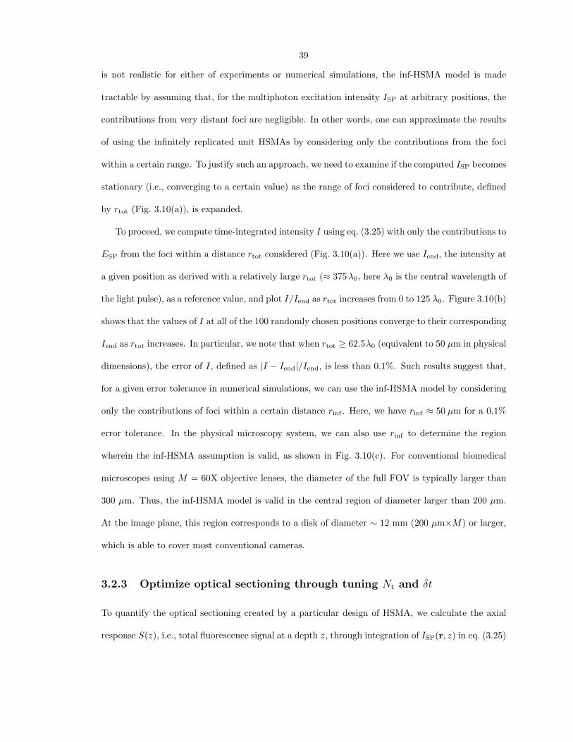
39

is not realistic for either of experiments or numerical simulations, the inf-HSMA model is made

tractable by assuming that, for the multiphoton excitation intensity ISP at arbitrary positions, the

contributions from very distant foci are negligible. In other words, one can approximate the results

of using the infinitely replicated unit HSMAs by considering only the contributions from the foci

within a certain range. To justify such an approach, we need to examine if the computed ISP becomes

stationary (i.e., converging to a certain value) as the range of foci considered to contribute, defined

by rtot (Fig. 3.10(a)), is expanded.

To proceed, we compute time-integrated intensity I using eq. (3.25) with only the contributions to

ESP from the foci within a distance rtot considered (Fig. 3.10(a)). Here we use Iend, the intensity at

a given position as derived with a relatively large rtot (≈ 375λ0, here λ0 is the central wavelength of

the light pulse), as a reference value, and plot I/Iend as rtot increases from 0 to 125 λ0. Figure 3.10(b)

shows that the values of I at all of the 100 randomly chosen positions converge to their corresponding

Iend as rtot increases. In particular, we note that when rtot ≥ 62.5λ0 (equivalent to 50 µm in physical

dimensions), the error of I, defined as |I − Iend|/Iend, is less than 0.1%. Such results suggest that,

for a given error tolerance in numerical simulations, we can use the inf-HSMA model by considering

only the contributions of foci within a certain distance rinf . Here, we have rinf ≈ 50 µm for a 0.1%

error tolerance. In the physical microscopy system, we can also use rinf to determine the region

wherein the inf-HSMA assumption is valid, as shown in Fig. 3.10(c). For conventional biomedical

microscopes using M = 60X objective lenses, the diameter of the full FOV is typically larger than

300 µm. Thus, the inf-HSMA model is valid in the central region of diameter larger than 200 µm.

At the image plane, this region corresponds to a disk of diameter ∼ 12 mm (200 µm×M) or larger,

which is able to cover most conventional cameras.

3.2.3 Optimize optical sectioning through tuning Nt and δt

To quantify the optical sectioning created by a particular design of HSMA, we calculate the axial

response S(z), i.e., total fluorescence signal at a depth z, through integration of ISP(r, z) in eq. (3.25)

40

rtot

(a)

!"!

!""

!"!

I/I end

#$%&'()*+

" ,-./ !-/".000

!

!.""!

12$2&3

"4

#56+)1&'()*+

(b)

rinf

(c)

Figure 3.10: (a) The time-integrated intensity I at a particular position is numerically obtained bytaking into account the contributions of foci within distance rtot. The dark area with an array ofbright spots indicates the calculated intensity distribution. The faded grid patterns shows the loca-tions of microlenses when projected to the specimen plane of the microscope. (b) The convergenceof I for 100 randomly picked positions (upper panel: log scale; lower panel: linear scale). Eachcurve represents I/Iend as a function of rtot (see text) at a particular position. The analysis hasbeen repeated 10 times; all results show similar convergence. (c) The area for the inf-HSMA modelis valid can be determined by rinf and the size of the whole FOV of the microscope.

41

!"#

!"$

!"%

!"&

'

()*+,-./-0/-1.2304)

dfoci

0.4 0

1

1

'! 5 ! 5 '!!

!"#

!"$

!"%

!"&

617!8

dfoci

0.8 0

1

1

;<?$

;<?9

;<?'%

;<?#5

;<?:%

;<?$9

()*+,-./-0/-1

.2304)

(c)

(b)

6@A

=

6@A

dfoci≈ d

0

dfoci≈ 2d

0

Figure 3.11: Axial responses S(z) of various (Nt, ∆t) sets

over the transverse coordinates, as

S(z) =

∫ISP(r, z)d2r. (3.26)

Experimentally, S(z) corresponds to the detected fluorescence signal from a thin fluorescent layer

placed at a depth z.

To determine the choice of (Nt, ∆t) that produces the most efficient optical sectioning, we

evaluate S(z) and the ratio of out-of-focus and in-focus signal, Sout/Sin (see Fig. 3.12 for illustration),

for various sets of Nt and ∆t (constrained by eq. (3.21)) with two interfocal spacings, dfoci(≡ d/M ,

where M is the magnification of the microscopy system) ≈ d0 and 2 d0.

Because of the square geometry of our HSMAs, we examine Nt = 22, 32, 42, ... and 92. Analyzing

Sout/Sin reveals that the decay of the out-of-focus excitation significantly slows down between Nt =

16 and 64, corresponding to ∆t ≈ 30-8 fs (i.e., τ0-1/4 τ0), for various arrangement of the distinct

time-delay steps (Fig. 3.13). These results suggest that the optical sectioning for a fixed ∆ttot is

optimized when ∆t is slightly smaller than τ0. Further reducing ∆t (equivalent to increasing Nt

(eq. (3.21))) can complicate the fabrication of the HSMAs without major improvement of optical

sectioning. In addition, increasing dfoci leads to weaker out-of-focus excitation and a less complex

42

!" # " # !""

"$%

"$&

"$'

"$(

!

)*+",

-./012342542*36758.

!" # " # !""

"$%

"$&

"$'

"$(

!

)*+",

-./012342542*36758.

!" # " # !""

"$%

"$&

"$'

"$(

!

)*+",

-./012342542*36758.

In-focus region: area inside of half maximums

In-focus signal (Sin) Out-of-focus signal (Sout)

Figure 3.12: Illustration of in-focus signal and out-of-focus signal.

axial excitation profile S(z) (Fig. 3.11).

3.2.4 Experimental verification of reduction of out-of-focus excitation by

HSMA

To verify the predicted out-of-focus excitation reduction in HSMA-based temporal focusing, we

fabricated a height-staggered plate and experimentally conducted the axial response measurement

(Fig. 3.14) by imaging a thin layer of fluorescent dye with the microscope objective translated

through 200 sequential depths at 0.1-µm intervals. We made this plate using a multi-exposure

protocol of photolithography (Fig. 3.15). In this protocol, the first layer of photoresist is spin-coated

on the base plate and then exposed to UV light under a photo-mask, followed by soft baking of

the exposed photoresist. Such a procedure is repeatedly conducted for Nt − 1 times to build up an

Nt-level height-staggered plate. To guarantee the flatness of the surface, the photoresist is softly

baked but not developed after intermediate exposures. Development was performed only after all

the spin-coatings, exposures and soft-bakings were accomplished.

The height staggering we used for experiments has an Nt = 9 and dfoci ≈ 2d0. Although our

simulations suggest that an Nt equal to or greater than 16 optimizes optical sectioning, we chose an

43

Nt

4 9 16 25 36 49 64 810

10

20

30

Nt

Sout/Sin

30

Raster

dfoci

dfoci

Nt

4 9 16 25 36 49 64 810

10

20

30

Nt

Sout/Sin

* t 170/N

t

Diagonal

4 9 16 25 36 49 64 810

10

20

30

Nt

Sout/S

in

30

Jumping spiral

*All heights plotted

linearly in gray scale d

foci ≈ d

0

dfoci ≈ 2d

0

Figure 3.13: The ratios of out-of-focus signal to in-focus signal under three different spatial arrange-ments of distinct time-delay steps.

! " !"

"#$

"#%

"#&

"#'

!

()*µ+,

-./012342542)36758.

! " !"

"#$

"#%

"#&

"#'

(

)*+µ,-

./0123453653*47869/

Dense Multifocal 2-Photon Excitation

Dense Time-Multiplexed Multifocal 2-Photon Excitation

1-Photon Multifocal Excitation

Experiment Simulation

Figure 3.14: The numerically simulated and experimentally measured (excitation) axial responses ofdense multifocal 2-photon excitation (blue), dense time-multiplexed multifocal 2-photon excitation(green), single-photon multifocal illumination (red). The interfocal distance dfoci ≈ 2d0 for bothsimulations and experiments. The height-staggering used for simulations and experiments has Nt =9. The emission filter used for experiments has a transmission window at 554 ± 105 nm.

44

Figure 3.15: Illustration of the multi-exposure protocol we used to fabricate the height-staggeredplate. The thickness of each SU-8 layer is ∼30 µm.

Nt = 9 out of fabrication simplicity. After all, the results of simulations show that the improvement

of optical sectioning by using Nt = 16 over Nt = 9 is around 10% in terms of the ratio of out-of-

focus signal to in-focus signal, while making a 9-level height-staggering plate is nearly 27 times easier

than a 16-level one. This is because the success of each repetitive procedure is independent of one

another, but the failure of any single one means the failure of the entire fabrication. The fluorescent

thin layer was made by sandwiching a tiny drop of a fluorescent dye between a #1.5 coverslip

and a non-fluorescent quartz microscope slide (Ted Pella, Inc.). The fluorescent dye was diluted 3

times from a saturated 1,8-ANS solution of dimethylformamide. The thickness of the thin layer was

estimated as ≤ 0.5 µm by dividing the volume of the dye drop with the coverslip area. In Fig. 3.14

the axial response of multifocal 2-photon excitation with only a microlens array is denoted as dense

multifocal 2-photon excitation (blue line), while 2-photon excitation with a microlens array and

height-staggered plate is denoted as dense time-multiplexed multifocal 2-photon excitation (green

line). Although our usage of the heigh-staggered plate results from a context different from time

45

multiplexing of multifocal multiphoton microscopy, we named our technique so in order to credit

it to the very first concept of introducing time multiplexing to reduce interfocal interferences at

out-of-focus regions. The presented result of experiments are averaged out of 15 repeats.

Figure 3.14 shows qualitatively good agreement between the results of experiments and simu-

lations. The quantitative difference between experiments and simulations is mostly caused by our

usages of scalar field-based simulations rather than vectorial field-based ones.

3.2.5 Enhance optical sectioning by implementing structured illumina-

tion microscopy

As discussed in Section 3.2, our approach allows moderate out-of-focus excitation in order to keep

dfoci small and image acquisition fast and simple. To further enhance the capability of optical

sectioning of our technique, fortunately, the periodic multifocal pattern can be readily utilized for

structured illumination microscopy, which can remove out-of-focus signal from acquired images. Here

we demonstrate the optical performances of such implementation by numerical simulations as well

as experimental measurements. Structured illumination microscopy relies on the post processing of

multiple images, each noted as Iimg. Because the emitted fluorescence (wavelength assumed to be

∼ 0.56λ0) from the specimen is generally incoherent, as discussed in Section 1.1, we can estimate Iimg

from a convolution of the excitation intensity profile ISP and the intensity PSF of the microscopy

system, IPSF [20], as

Iimg(r′) =

∫ISP(r, z) f(r, z) IPSF(r′ +Mr,M2z)d2r dz, (3.27)

where f is the concentration distribution of the fluorophore in the specimen. To quantify the optical-

sectioning effect, we assume that the specimen is an ideal thin fluorescent film placed at z = zf , i.e.,

f(r, z) = δ(z − zf ). eq. (3.27) then becomes

Iimg(r; zf ) =

∫ISP(r′, zf ) IPSF(r +Mr′,M2zf )d2r′. (3.28)

46

! " !#"

$

#"%

#"&

#"#

#""

'()µ*+

,-./01231431(25647-

!"!

!""

!"#

!"$

!"%

!"!

!""

&'(µ)*

+,-./0120320'14536,

Single-Point-Scanning 2-Photon Excitation

Dense Time-Multiplexed Multifocal 2-Photon Excitation

Dense Time-Multiplexed Multifocal 2-Photon Excitation + SIM

Semi-log Log-log

Figure 3.16: Simulated axial responses of single-point-scanning 2-photon excitation microscopy(blue), dense time-multiplexed multifocal multiphoton microscopy with (red) and without (green)structured illumination microscopy, in semi-log and log-log scales. The wavelength of the emittedfluorescence is set to be ∼510 nm. dfoci ≈ 2d0.

Conventional structured illumination microscopy takes 3 shifts of the 1-dimension periodic pattern;

each step is 1/3 of the period of the pattern [3]. In our case, the periodicity of ISP is 2-dimensional.

We thus use 3-by-3 shifts (Iimg1, Iimg2, ..., Iimg9 denote the obtained images) and apply the post-

processing routine of structured illumination microscopy to extract the optically sectioned images

ISIM =

√√√√ 9∑i=1

9∑j=1

(Iimgi − Iimgj)2. (3.29)

We then substitute ISP in eq. (3.26) with ISIM to evaluate the overall strength of optical sectioning

(Fig. 3.16).

The results show that after applying structured illumination microscopy, we can reproduce the

1/z2 axial response as observed in single-point-scanning 2-photon excitation microscopy. From the

results of simulations we also found that the axial resolution of our technique has a ∼1.3-fold im-

provement over that of a single-point-scanning confocal microscope (Fig. 3.17).

Although confocal microscopy is conventionally regarded as the standard technique for achieving

diffraction-limited optical sectioning, we should note that this is not a fundamental breakthrough

of diffraction limit. Similar performance can be expected if one implements structured illumination

47

! " !"

"#!

"#$

"#%

"#&

'

()*µ+,

-./012342542)36758.

! "#$ " "#$ !"

"#%

"#&

"#'

"#(

!

)*+µ,-

./0123453653*47869/

Simulation Experiment

!"#$%&'()"#*'!+,##"#$-.'(/)*)#-0"+1)2+)34-

!"#$%&'()"#*'!+,##"#$-5)#6)+,%-0"+1)2+)34-

7&#2&-8"9&'0:%;3%&<&=-0:%;6)+,%-.'(/)*)#-0"+1)2+)34->-!?0-

Figure 3.17: Comparisons of axial responses of single-point-scanning 2-photon microscopy (blue),single-point-scanning confocal microscopy (green) and dense time-multiplexed multifocal 2-photonmicroscopy in conjunction with structured illumination microscopy (red) in both numerical sim-ulations and experiments. The simulated/experimental FWHMs of each techniques are 0.56/1.04µm for sing-point-scanning 2-photon microscopy, 0.29/0.79 µm for single-point-scanning confocalmicroscopy, and 0.24/0.56 µm for dense time-multiplexed multifocal 2-photon microscopy in con-junction with structured illumination microscopy. The wavelengths of excitation and emission insimulations of single-point-scanning confocal microscopy are both 510 nm. The emission filter usedfor experiments has a transmission window at 510 ± 5 nm.

48

microscopy on conventional multifocal multiphoton microscopy or multifocal confocal microscopy,

and such an improvement can be understood as a combination of two different, independent optical-

sectioning mechanisms [37]. The advantage of implementing structured illumination microscopy

on our system is simplicity. Combining structured illumination microscopy with multifocal multi-

photon/confocal microscopy requires additional telescoping between the structured pattern and the

spinning disk, which is by itself a complicated opto-mechanic device. On the contrary, performing

structured illumination microscopy on our system requires only acquire individual image at each

translation/scanning step, which can be easily edited into several microscope management software

programs.

We further simulate the images of a virtual 3-dimensional object obtained by the different imaging

techniques (Fig. 3.18) to illustrate the optical sectioning of our proposed dense time-multiplexed

multifocal multiphoton microscopy in conjunction with structured illumination microscopy (denoted

as dTMMMM + SIM). Compared with conventional epifluorescence microscopy (Fig. 3.18(b), Epi),

the images obtained before structured-illumination post processing (denoted as dTMMMM) shows

the ability of intrinsic optical sectioning. In the log-scale intensity plot (Fig. 3.18(c)), dTMMMM +

SIM has the highest signal contrast between fluorescent and non-fluorescent areas, consistent with

the results in Fig. 3.17. Moreover, the reconstructed 3-dimensional views show that dTMMMM +

SIM successfully reproduces the details of the object (Fig. 3.18(d)).

To demonstrate the capability of imaging living biological systems, we also performed optical sec-

tioning on living C. elegans using our proposed technique (Fig. 3.19, dTMMMM + SIM). In Fig. 3.19

we also compare the z-sequential images obtained under our technique and conventional epifluores-

cence microscopy. The imaged C. elegans on both microscopes have two mechanosensory neurons

separated by ∼5 µm on z axis, and we can see that our technique shows clear axial segregation of

the two neurons.

We should note that the post processing of structured illumination microscopy introduced here,

i.e., the 9-frame imaging procedure and eq. (3.29), is not the only way to remove out-of-focus signal

from the obtained images Iimg. Other methods using a high-spatial-frequency illumination pattern

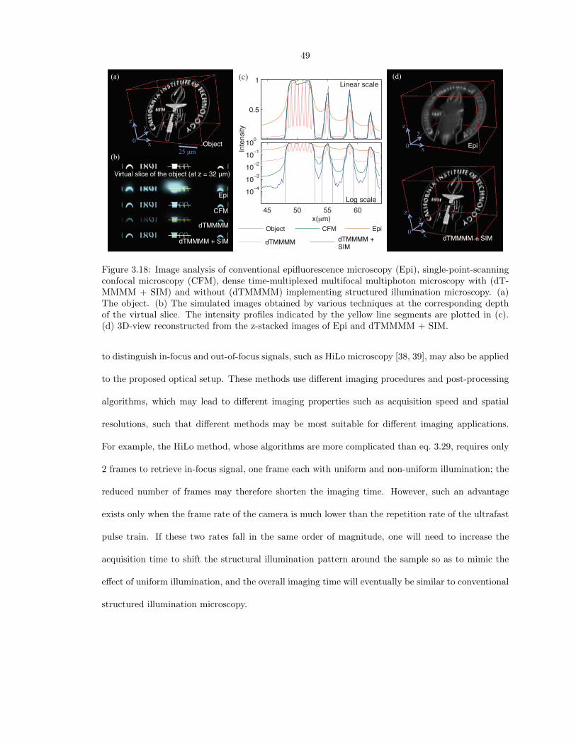
49

!"#

$%&'()*+,-).(

/# #! ## 0!

$!/

$!1

$!2

$!$

$!!

34µ56

7'8(',&89

%:;+,-).(+

+

(c)

z

x

y

25 µm

Virtual slice of the object (at z = 32 μm)

0

dTMMMM + SIM

(a)

(b)

Object

Epi

CFM

dTMMMM

Epi

(d)

dTMMMM + SIM

z

x

y

0

z

x

y

0 <=>(-8 ?@A BC&

BC& AD EEAE ADF7 EEAEdTMMMM dTMMMM + SIM

Figure 3.18: Image analysis of conventional epifluorescence microscopy (Epi), single-point-scanningconfocal microscopy (CFM), dense time-multiplexed multifocal multiphoton microscopy with (dT-MMMM + SIM) and without (dTMMMM) implementing structured illumination microscopy. (a)The object. (b) The simulated images obtained by various techniques at the corresponding depthof the virtual slice. The intensity profiles indicated by the yellow line segments are plotted in (c).(d) 3D-view reconstructed from the z-stacked images of Epi and dTMMMM + SIM.

to distinguish in-focus and out-of-focus signals, such as HiLo microscopy [38, 39], may also be applied

to the proposed optical setup. These methods use different imaging procedures and post-processing

algorithms, which may lead to different imaging properties such as acquisition speed and spatial

resolutions, such that different methods may be most suitable for different imaging applications.

For example, the HiLo method, whose algorithms are more complicated than eq. 3.29, requires only

2 frames to retrieve in-focus signal, one frame each with uniform and non-uniform illumination; the

reduced number of frames may therefore shorten the imaging time. However, such an advantage

exists only when the frame rate of the camera is much lower than the repetition rate of the ultrafast

pulse train. If these two rates fall in the same order of magnitude, one will need to increase the

acquisition time to shift the structural illumination pattern around the sample so as to mimic the

effect of uniform illumination, and the overall imaging time will eventually be similar to conventional

structured illumination microscopy.

50

z = 0 µm

z = 12 µm

z = 13 µm

z = 10 µm

z = 11 µm

z = 9 µm

z = 8 µm

z = 7 µm

z = 6 µm

z = 5 µm

z = 4 µm

z = 3 µm

z = 2 µm

z = 1 µm

dTMMMM+SIM Epi

Figure 3.19: Images of sequential depths of C. elegans obtained under dense time-multiplexed mul-tifocal multiphoton microscopy in conjunction with structured illumination microscopy (dTMMMM+ SIM) and conventional epifluorescence microscopy (Epi). The imaged strain (ZDLS5) expressesgreen fluorescent protein in its mechanosensory neurons. Each translation/scanning step is exposedfor 100 ms; 3-by-3 translation/scanning steps were used to construct a sectioning image. Scale bar:20 µm.

51

3.2.6 Brief summary

Our numerical simulations and experiments shows that dTMMMM + SIM can provide optical

sectioning by combining temporal focusing/time multiplexing and structured illumination in a simple

optical setup, and achieves an axial resolution finer than single-point-scanning confocal microscopy.

Our analysis provides the design guide of HSMAs with small time-delay increments; the dimensions

of the proposed HSMAs are compatible with standard biomedical microscopes, and feasible for

existing fabrication methods. In contrast to conventional structured illumination microscopy, the

intrinsic sectioning of our method can reduce photobleaching and increase the signal-to-noise ratio

of the processed images.

Compared with multifocal multiphoton/confocal microscopy, our technique has a denser spacing

of foci (> 10 foci per 102-focus area), and thus has greater potential in high-speed imaging. In

addition to the fine axial resolutions, the lateral resolution of our technique can also be enhanced

via utilization of the periodic excitation structures and Fourier analysis of the obtained images [40].

Moreover, our technique can use the pulse train generated by ultrafast amplifiers, thereby yielding

a sufficient signal level and moderate impact on the specimen at high acquisition rates, as demon-

strated in our previous diffuser-based temporal focusing setup [36]. Taken together, we have shown

that dense time-multiplexed multifocal multiphoton microscopy in conjunction with structured il-

lumination microscopy has the potential to achieve (better-than-conventional) diffraction-limited,

high-frame-rate volumetrc imaging with a simple, wide-field optical design.

3.3 High-degree time-multiplexed multifocal multiphoton mi-

croscopy by a length-staggered fiber bundle

As discussed in previous sections, our HSMA-based temporal focusing/time-multiplexing does not

provide the standard 1/z2 axial response because of the moderate out-of-focus excitation. The

only way to further reduce this out-of-focus excitation is to employ even larger total time delays

∆ttot. However, as we mentioned previously, it is not practical to use the conventional pillar-like

52

structures to create high-degree time multiplexing because of the nature of diffraction of light waves

propagating in free space. Such diffraction leads to the divergence of a propagating beam, which

can cause a leakage of light between neighboring pillars, thereby degrading temporal separation and

optical sectioning. We show in the last section that such a divergence depends on the cross-sectional

area of the pillars, and that having a negligible light leakage requires:

A ≥ λ0 ∆hmax, (3.30)

where λ0 is the central wavelength of the light pulse, A is the cross-sectional area of a single pillar

and ∆hmax is the maximal height difference among the pillars. Using eq. (3.30) to estimate the

dimensions of a time-multiplexing device that can perform scanningless wide-filed imaging with an

∼100-fs duration ultrafast pulse train, we found that it requires ∆hmax to be > 30 mm and the

cross-sectional area of the entire device to be larger than 100 cm2 [37]. Fulfilling both of these

requirements on one optical device is far beyond the fabrication capability of current optical-quality

manufacturing techniques. Alternatively, this light leakage is avoidable if the ends of the pillars

can be aligned on individual planes perpendicular to the optical axis of the imaging system, e.g., a

conventional microlens array, which apparently provides no time multiplexing.

In this section we present a new design for a time-multiplexing device, one that can be easily

manufactured and that creates a high degree of time multiplexing without the concerns of light

leakage between neighboring time-delay channels. Our device consists of a bundle of optical fibers

of various lengths, wherein time multiplexing is created by the relative length differences among the

fibers. To avoid the aforementioned light leakage, we aligned the ends of all the fibers at the input

and output planes, while the length differences were compensated by slight bending of the fibers

(Fig. 3.20).

Because of the length differences of the optical fibers, input light pulses that simultaneously enter

53

z = ze (lab frame) z = zi (lab frame)

Camera

Fiber array

Objective

Tube lens

Lens

Beamsplitter

Sample

ei

Figure 3.20: Schematic of the optical system. After a light pulse passes through the fiber bundle,multiple light pulses are generated with spatial and temporal separations amongst one another,and create a plane of foci at the focal plane of the microscope objective. Because of the temporalseparation, the optical properties of each focus can be considered identical to the conventionalsingle-focus multiphoton microscopy [5]. The fluorescence emitted within the excited plane are thencollected by the microscope objective and routed to a camera for wide-field imaging. The dashedlines show the central traces of the light pulses passing through individual optical fibers, and theshaded region exemplifies the beam profile of a light pulse exiting an optical fiber. The inset is aphotograph of the actual fiber bundle.

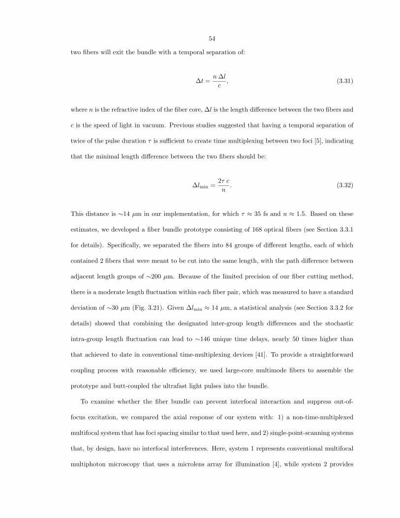
54

two fibers will exit the bundle with a temporal separation of:

∆t =n∆l

c, (3.31)

where n is the refractive index of the fiber core, ∆l is the length difference between the two fibers and

c is the speed of light in vacuum. Previous studies suggested that having a temporal separation of

twice of the pulse duration τ is sufficient to create time multiplexing between two foci [5], indicating

that the minimal length difference between the two fibers should be:

∆lmin =2τ c

n. (3.32)

This distance is ∼14 µm in our implementation, for which τ ≈ 35 fs and n ≈ 1.5. Based on these

estimates, we developed a fiber bundle prototype consisting of 168 optical fibers (see Section 3.3.1

for details). Specifically, we separated the fibers into 84 groups of different lengths, each of which

contained 2 fibers that were meant to be cut into the same length, with the path difference between

adjacent length groups of ∼200 µm. Because of the limited precision of our fiber cutting method,

there is a moderate length fluctuation within each fiber pair, which was measured to have a standard

deviation of ∼30 µm (Fig. 3.21). Given ∆lmin ≈ 14 µm, a statistical analysis (see Section 3.3.2 for

details) showed that combining the designated inter-group length differences and the stochastic

intra-group length fluctuation can lead to ∼146 unique time delays, nearly 50 times higher than

that achieved to date in conventional time-multiplexing devices [41]. To provide a straightforward

coupling process with reasonable efficiency, we used large-core multimode fibers to assemble the

prototype and butt-coupled the ultrafast light pulses into the bundle.

To examine whether the fiber bundle can prevent interfocal interaction and suppress out-of-

focus excitation, we compared the axial response of our system with: 1) a non-time-multiplexed

multifocal system that has foci spacing similar to that used here, and 2) single-point-scanning systems

that, by design, have no interfocal interferences. Here, system 1 represents conventional multifocal

multiphoton microscopy that uses a microlens array for illumination [4], while system 2 provides

55

−100 −50 0 50 1000

5

10

15

20

25

Length difference (µm)

Co

unts

Figure 3.21: Length distribution of fibers that were meant to be cut into the same length. Toquantify the length stochasticity induced by our fiber cutting procedures, we measured the lengthsof 160 fibers that were prepared through the same procedures, and plot here the histogram of thedifferences between the measured lengths and the designated length. The distribution of lengthdifferences is in good agreement with a Gaussian distribution of a 30 µm standard deviation (blueline).

a quantitative comparison to conventional single-point-scanning multiphoton excitation microscopy

[2]. The axial responses of each system were measured by imaging the same thin fluorescent layer

at sequential depths around the focal plane of the microscope objective. To fairly compare the out-

of-focus excitation of our time-multiplexed system and a non-time-multiplexed system, we chose a

microlens array where the aperture formed by single microlens exhibited an axial-response FWHM

(Fig. 3.22, red broken line) similar to that measured under single-fiber illumination (see Section 3.3.4

for details). The results show that the axial response of our fiber-bundle system resembles those of

single-point-scanning systems illuminated with either a single microlens or an optical fiber (Fig. 3.22),

and therefore confirm that the length differences of the fibers can indeed create sufficient temporal

separations among the spatially neighboring foci to prevent out-of-focus excitation. Using multimode

fibers, however, can create an axial response that is a mixture of the axial responses of several optical

modes. As higher-order modes generally exhibit greater focal depths, such mode mixing should lead

to a broader peak in the axial response curve. Indeed, the axial response curve measured in the

system with single-fiber illumination showed a FWHM of ∼ 1.8 µm (Fig. 3.22, black broken line), in

contrast with the ∼ 0.9-µm FWHM in an optimized conventional single-point-scanning multiphoton

excitation microscope using the same objective [1].

To further demonstrate the fast optical-sectioning capability of our system, we imaged fluorescent

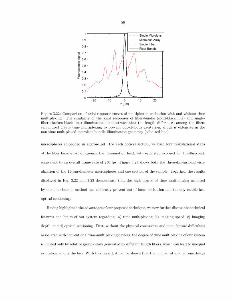
56

−20 −10 0 10 200

0.1

0.2

0.3

0.4

0.5

0.6

0.7

0.8

0.9

1

z (µm)

Flu

ore

sce

nce s

ignal

Single Microlens

Microlens Array

Single Fiber

Fiber Bundle

Figure 3.22: Comparison of axial response curves of multiphoton excitation with and without timemultiplexing. The similarity of the axial responses of fiber-bundle (solid-black line) and single-fiber (broken-black line) illumination demonstrates that the length differences among the fiberscan indeed create time multiplexing to prevent out-of-focus excitation, which is extensive in thenon-time-multiplexed microlens-bundle illumination geometry (solid-red line).

microspheres embedded in agarose gel. For each optical section, we used four translational steps

of the fiber bundle to homogenize the illumination field, with each step exposed for 1 millisecond,

equivalent to an overall frame rate of 250 fps. Figure 3.23 shows both the three-dimensional visu-

alization of the 15-µm-diameter microspheres and one section of the sample. Together, the results

displayed in Fig. 3.22 and 3.23 demonstrate that the high degree of time multiplexing achieved

by our fiber-bundle method can efficiently prevent out-of-focus excitation and thereby enable fast

optical sectioning.

Having highlighted the advantages of our proposed technique, we now further discuss the technical

features and limits of our system regarding: a) time multiplexing, b) imaging speed, c) imaging

depth, and d) optical sectioning. First, without the physical constraints and manufacture difficulties

associated with conventional time-multiplexing devices, the degree of time multiplexing of our system

is limited only by relative group delays generated by different length fibers, which can lead to unequal

excitation among the foci. With this regard, it can be shown that the number of unique time delays

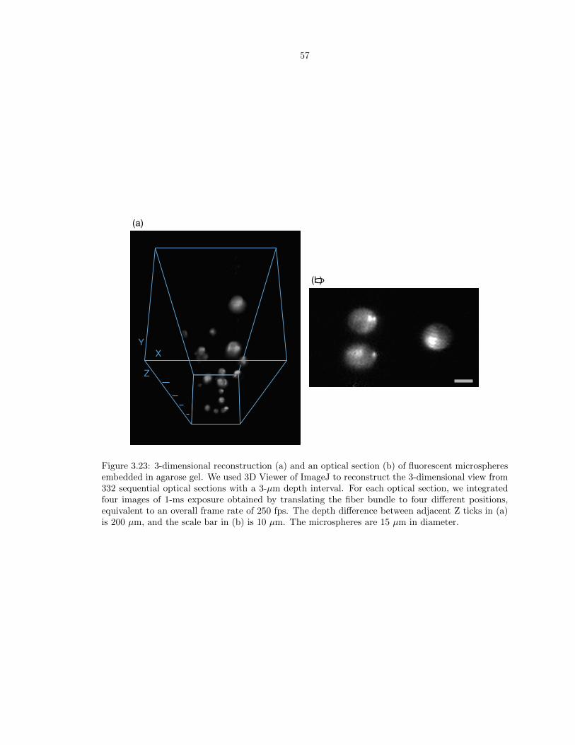
57

(a)

(b)

Y

X

Z

Figure 3.23: 3-dimensional reconstruction (a) and an optical section (b) of fluorescent microspheresembedded in agarose gel. We used 3D Viewer of ImageJ to reconstruct the 3-dimensional view from332 sequential optical sections with a 3-µm depth interval. For each optical section, we integratedfour images of 1-ms exposure obtained by translating the fiber bundle to four different positions,equivalent to an overall frame rate of 250 fps. The depth difference between adjacent Z ticks in (a)is 200 µm, and the scale bar in (b) is 10 µm. The microspheres are 15 µm in diameter.

58

is bounded by:

NTM ≤ (n

2 β c |D|) · τ, (3.33)

where D is the dispersion parameter of the optical fiber, and β is the transformation constant of

transform-limited light pulses (see Section 3.3.5 for details). In our system where τ ≈35 fs and

D ≈ −116 ps/nm/km, we obtained the upper bound of NTM to be ∼1,500, which is much larger

than the aforementioned ∼300 unique time delays required for scanningless imaging.

Second, for the speed of imaging, the instrumental limitations are the repetition rate of the

ultrafast pulse train, the frame rate of the camera, and the translation rate of fiber bundle – if

translation is required for homogeneous illumination (translation is not absolutely necessary for

fiber bundles made of closely spaced, low numerical-aperture fibers). To date, commercially available

ultrafast oscillators can provide repetition rates up to 1-10 GHz at average powers of over a Watt,

while if larger single pulse energies are needed, regenerative amplifiers can produce ≥mJ pulses with

repetition rates into the many tens of kHz. Scientific-grade CMOS cameras already exceed rates

of 1,000 fps with limited numbers (∼100-by-100) of pixels, and further advances in frame rate and

image size can be expected. For fiber-bundle translation, fast mechanical stages typically achieve

step rates of ∼1 kHz; for even faster operation, galvanometric mirrors that translate the foci at rates

higher than 50 kHz can be used, in an optical design similar to a previously demonstrated multifocal

system [42]. Thus, the imaging speed of our technique can be pushed well beyond 1,000 fps even

with the limits of currently available equipment and techniques.

Third, the imaging depth of our technique could be more significantly impaired by optical scatter-

ing and aberration induced by the sample compared with the non-imaging detection of conventional

single-point-scanning multiphoton microscopy. This occurs because our technique, like SPIM and

structured illumination microscopy, requires imaging the emitted light onto the sensor array of a

camera. Such a disadvantage may be mitigated by spatial registration of the signal, i.e., assigning

the signal collected by certain pixels of the sensor array to individual foci, and utilizing the spatial

information associated with the foci to reconstruct the entire image [42]. One can also transform

such a methodology into frequency registration of the signal, i.e., encoding the amplitudes of foci

59

with various frequencies and reconstructing the image through frequency analysis of the collected flu-

orescence signal [43]. In addition, if the fluorescence signal is strong enough, the scattering-induced

blur can be numerically removed by applying structured illumination[3] using the foci pattern; this

approach may also enhance the axial resolution [37, 44, 45].

Fourth, for the optical sectioning capability, the optimized axial resolution of our technique is

equivalent to that of conventional single-point-scanning multiphoton excitation microscopy. Such an

optimization requires the beam exiting the fiber to be collimated to the microscope objective with

a flat wavefront and uniform amplitude distribution, suggesting that a single-mode fiber bundle

assembly is highly preferred. Achieving efficient light coupling with such a single-mode-fiber bundle

requires high-precision alignment and assembly of a light-coupling microlens array with the fiber-

array bundle. Fortunately, the technology for this demanding task has recently become commercially

available due to the fast-growing demands of highly parallel optical communication [46, 47].

In summary, we demonstrate a simple technique that has achieved the highest degree of time

multiplexing ever demonstrated in multifocal multiphoton microscopy. We show that by introducing

length differences within a bundle of optical fibers, the induced time multiplexing efficiently prevents

the out-of-focus excitation even among densely spaced foci. Upon optimization, our technique will

surpass currently available wide-field optical-sectioning fluorescence microscopies in terms of axial

resolution and system simplicity, and achieve spatial resolutions equivalent to conventional single-

point-scanning multiphoton excitation microscopy. With an imaging speed potentially beyond 1,000

fps, we believe that our technique will become a powerful imaging tool in future life science research.

In following sections we describe certain technical details of our fiber bundle-illumination method.

3.3.1 Fiber bundle manufacturing

As described in the main text, we assembled the fiber bundle with large-core multimode fibers (core

diameter ≈62.5 µm and cladding diameter ≈125 µm, dispersion coefficient ≈-116.4 ps/nm/km,

YOFC R©) of various lengths. To cut the optical fibers into designated lengths, we fixed fibers on

a precision translational stage to adjust the lengths, and cut the fibers with a cleaver next to the

60

stage. When assembling the fibers, both ends of the bundle were aligned perpendicular to the optical

axis, as shown in Fig. 3.20. The length differences were compensated by slightly bending the fibers

– the optical bending loss is negligible due to the relatively short length differences (∆lmax ≈ 17

mm) compared with the average length of the fiber bundle (≈200 mm). After assembly, the physical

strength of the fiber bundle was further enhanced by applying UV-cured epoxy near the ends of the

fibers, followed by polishing and ultrasonic cleaning at both ends of the fiber bundle.

3.3.2 Statistical analysis of the degree of time multiplexing

To estimate the degree of time multiplexing created by our fiber preparation, we numerically simu-

lated the length distribution of the resulting fiber bundle. As shown in Fig. 3.21, our fiber cutting

method produced a Gaussian-like length distribution with a standard deviation of ∼30-µm. To in-

clude such stochasticity, we added a Gaussian random variable with a mean at 0 µm and a standard

deviation of 30 µm to the lengths of the fibers in each length group. We then compared the length

differences among all 168 fibers in the bundle and determined the number of unique time delays.

Specifically, we reduced 168 by the number of fibers that have a length difference less than ∆lmin

with another fiber in the bundle to obtain the number of unique time delays (∆lmin indicates the

minimal length difference for creating two unique time delays, set to be 14 µm in the simulation).

By averaging 1,000 simulations we concluded that ∼ 146 ± 4 unique time delays can be produced

by our fiber bundle preparation.

3.3.3 Development of the optical system

The light source of our system is a Ti:Sapphire ultrafast regenerative amplifier (Legend Elite-USP-

1k-HE, Coherent, Inc.) seeded with an ultrafast oscillator (Mantis-5, Coherent, Inc.), and is butt-

coupled into the fiber bundle. The repetition rate and pulse duration of the ultrafast pulse train are

∼1 kHz and ∼35 fs, respectively. In our infinity-corrected optical setup (Fig. 3.20), the output end

of the fiber bundle was placed at the focal pane of the collimation lens (f = 150 mm plane-convex

lens, KPX100AR.16, Newport Corp.). The temporally and spatially separated pulses entered an

61

inverted microscope frame (IX71, Olympus) through its back port, and were reflected upward to the

microscope objectives by a beamsplitter (20RQ00UB.2 of customized dimensions, Newport Corp.).

The emitted fluorescence then formed an image on the sensor array of an electron-multiplying CCD

camera (iXon DU-885K, Andor). To measure the axial response shown in Fig. 3.22, we used a high

numerical aperture oil-immersion lens (PlanApo N 60X NA 1.42, Olympus) equipped with a high-

precision piezo stage (P-725 PIFOC R©, Physik Instrumente) for axial translation. The objective used

for acquiring the optical sections shown in Fig. 3.23 is a long-working-distance water-immersion lens

(XLUMPlanFL N 20X NA 1.00, Olympus). The number of translation steps for a homogeneous

illumination field was estimated as the square of the ratio of foci spacing to foci diameter. In our

system this ratio is ∼2, and thus we used a 22-step translation to image each depth in the sample.

3.3.4 Measurement of axial responses

We measured the axial response by imaging a thin fluorescent layer with the microscope objective

translated through 200 sequential depths at 0.3-µm intervals. The thin layer was made by sandwich-

ing a tiny drop of a fluorescent dye between a #1.5 coverslip and a non-fluorescent quartz microscope

slide (Ted Pella, Inc.). The fluorescent dye was diluted 3 times from a saturated 1,8-ANS solution of

dimethylformamide. The thickness of the thin layer was estimated as ≤ 1µm by dividing the volume

of the dye drop with the coverslip area. To measure the axial response of the non-time-multiplexing

microlens array, we replaced the fiber bundle with a square-microlens array (lens pitch ≈100 µm,

focal length ≈3 mm, Flexible Optical B.V.) of foci spacing similar to our fiber bundle. To have a

similar number of foci as those generated by our fiber bundle, we placed a mechanical iris in front

of the microlens array to partially block the excitation beam.

We conducted the single-fiber illumination by placing a 50 µm pinhole (P50S, Thorlabs, Inc.)

next to the input plane of the fiber bundle to selectively couple the excitation beam to a single

fiber. Because of the geometry of the mechanical mount and the high filling factor of the microlens

array, this pinhole-based technique required modest corrections to properly model a single-microlens

illumination geometry. To obtain the proper axial response curve equivalent to that of single-

62

microlens illumination, we first applied geometric optics calculations to estimate the equivalent

aperture formed by a single microlens, and then measured the axial response through a conventional

single-focus multiphoton microscope with the equivalent aperture placed in front of the back aperture

of the microscope objective. Each axial response curve was averaged from 15 separate z-scans.

3.3.5 Estimating the upper bound of the number of unique time delays

As described in the main text, the degree of time multiplexing of our technique is limited by the group

velocity dispersion of the ultrafast pulses within the fibers. The relative group delays generated by

different length fibers results in pulse duration variations in the exiting light pulses, which can lead

to unequal excitation among the foci. To mitigate this effect, the overall group delay ∆τGVD should

be restricted such that:

∆τGVD ≈ ∆lmax ·∆λ · |D| ≤ τ, (3.34)

where ∆lmax is the maximal fiber length difference in the bundle, ∆λ is the spectral span of a

transform-limited light pulse, and D is the dispersion parameter of the optical fiber. Under such

a restriction, the brightest foci will be no more than twice as bright as the darkest ones. Given

τ ≈ α/∆λ for transform-limited light pulses (β is a transformation constant), eqs. 3.32 and 3.34

suggest that the largest number of unique time delays is bounded by:

NTM ≈∆lmax

∆lmin≤ (

n

2 β c |D|) · τ. (3.35)

For commonly used near-infrared optical fibers and transform-limited Gaussian pulses, n2βc|D| is ∼50

fs−1 at λ0 ≈ 800 nm. In our system where τ ≈35 fs and D ≈ −116 ps/nm/km, we obtained that

NTM is upper-bounded by ∼1,500.

63

Chapter 4

Discussions and Conclusions

4.1 Discussions

Table 4.1 compares existing wide-field optical-sectioning techniques with our innovated ones. As

discussed in earlier chapters, conventional parallelization approaches using multifocal excitation im-

prove imaging speed limitedly because the distances among foci must be large enough to prevent

signal cross-talk among parallel channels. Further and for the same reason, the fast scanning of

multifocal patterns typically relies on a spinning microlens-array disk, which is technically elabora-

tive to manufacture. Multifocal confocal microscopy, in particular, requires precision alignment of

a microlens-array disk and a pinhole-array disk. Structured illumination microscopy, although pro-

vides a fundamental breakthrough in terms of parallelization (and thus imaging speeds), sacrifices

the dynamic range of the camera for unwanted out-of-focus signals and therefore leads to degraded

signal-to-noise ratio of the processed images. The separation of illumination and detection paths

makes SPIM uniquely suitable for imaging certain biological systems, but such an optical design

comes at prices of compromised axial resolution and inconvenient sample handling. Temporal fo-

cusing microscopy generalized the concept of time multiplexing to provide gap-less illumination and

optical sectioning at the same time. Nonetheless, its requirement of a high-order diffracted beam

for generating time delays greatly limits its applicability of imaging multiple fluorophores in the one

task.

Our innovated integration of dense time-multiplexed multifocal multiphoton microscopy and

64

structured illumination microscopy successfully overcomes the drawbacks of time-multiplexed multi-

focal multiphoton microscopy, structured illumination microscopy and temporal focusing, and mean-

while retains their advantages. The minor issue of such integration is that the out-of-focus excitation

remains at a moderate level, because the overall time delay is greatly limited by both the diffraction

of electromagnetic waves and micro-optics fabrication techniques. These difficulties are successfully

and fundamentally overcome by our novel design of the time-multiplexing device: a bundle of length-

staggered optical fibers. In order to provide sufficient pulse energy for exciting fluorophores in the

entire field of view at each pulse, our techniques require the usage of ultrafast amplifiers, which are

relatively pricey compared with other components of a conventional wide-field microscope. In this

regard, the ongoing innovations of fiber-based ultrafast amplifiers [48] can be expected to reduce the

overall costs and greatly enhance the availability of our techniques. Also, as mentioned previously,

the usages of low-repetition-rate amplified pulse trains can reduce light-induced photo-bleaching and

thermal-mechanical damages [17, 30].

4.2 Conclusions

In the history of the development of optical imaging techniques, optical microscopy systems have

been generally understood in a static manner, i.e., the optical properties of the microscopy systems

can be fully analyzed in time-independent geometrical optics-based and/or physical optics-based

models. In this thesis, we show that for multiphoton excitation fluorescence microscopy, there is

still certain space for investigations and innovations in temporal aspects, and this space is not quite

accessible if the dynamics of light pulses are over-simplified or even ignored as they usually were in

previous studies. Specifically, we investigate the possibilities of using 0-order diffraction to generate

time delays to reduce out-of-focus excitation in wide-field multiphoton excitation fluorescence mi-

croscopy. We discover the fundamental limitation, i.e., the inter-channel light leakage issue, of such

a methodology, and develop a physical optics-based simulation to optimize the optical systems under

this limitation. Furthermore, we also invent a new method, fiber-bundle illumination, to ultimately

resolve this limitation.

65

Our methods, especially the fiber-bundle illumination technique, can be the most powerful

optical-sectioning techniques among the existing ones upon optimization. It provides conceptu-

ally true scanningless illumination for high-frame-rate imaging, equivalent axial response to single-

point-scanning multiphoton excitation fluorescence microscopy, extremely low (average) excitation

intensity that is suitable for living-cell imaging, and at the same time its optical design is almost

as simple as a conventional far-field optical microscope. Such simplicity makes the technique itself

potentially low cost, easy to be used, maintained and even innovated by briefly trained persons.

We can therefore expect this technique to trigger more and more exciting inventions, explorations

and discoveries in various research fields such as fiber optics, bio-imaging, and ultimately, biology. I

believe that our techniques can greatly increase the availability and user-friendliness of diffraction-

limited volumetric fluorescence imaging techniques, and thus broadly benefit bio-imaging-related

researches in the near future.

66

Table 4.1: Features of wide-field optical-sectioning techniques. Ratio of in-focus to out-of-focusexcitation is estimated assuming that the microscope objective is a 60X NA 1.42 oil-immersion lens;the corresponding depth of field is ∼0.8 µm in the visible band. *Instrumentally achievable framerates. **The width of field of view is assumed to be 100 µm.

SystemSimplicity

FrameRate*

Ratio ofIn-Focus toOut-of-FocusExcitation

Specific Drawbacks

MultifocalConfocalMicroscopy

Moderate∼ 500 fpsor less

∼ 3 Fixed pinhole size

(Time-Multiplexed)MultifocalMultiphotonMicroscopy

Moderate∼ 500 fpsor less

∼ 3

StructuredIlluminationMicroscopy

High > 1, 000 fps ∼ 1/25 Degraded signal-to-noise ratio

SelectivePlaneIlluminationMicroscopy

Moderate > 1, 000 fps ∼ 1/2**Trade-off between axial resolutionand width of field of viewInconvenient for sample handling

TemporalFocusingMicroscopy

High > 1, 000 fps ∼ 1/12 [6]Wavelength-dependent optical pathRequires ultrafast amplifiers

DenseTime-MultiplexedMultifocalMultiphotonMicroscopy +SIM

High > 1, 000 fps ∼ 1/4 Requires ultrafast amplifiers

FiberBundle-BasedTime-MultiplexedMultifocalMultiphotonMicroscopy

High > 1, 000 fps ∼ 3 Requires ultrafast amplifiers

67

Bibliography

[1] J. B. Pawley, Handbook of biological confocal microscopy (Springer, New York, NY, 2006), 3rd

ed.

[2] W. Denk, J. H. Strickler, and W. W. Webb, “Two-photon laser scanning fluorescence mi-

croscopy,” Science 248, 73–6 (1990).

[3] M. Neil, R. Juskaitis, and T. Wilson, “Method of obtaining optical sectioning by using struc-

tured light in a conventional microscope,” Optics Letters 22, 1905–1907 (1997).

[4] J. Bewersdorf, R. Pick, and S. Hell, “Multifocal multiphoton microscopy,” Optics Letters 23,

655–657 (1998).

[5] A. Egner and S. Hell, “Time multiplexing and parallelization in multifocal multiphoton mi-

croscopy,” Journal of the Optical Society of America A-Optics Image Science and Vision 17,

1192–1201 (2000).

[6] D. Oron, E. Tal, and Y. Silberberg, “Scanningless depth-resolved microscopy,” Opt Express 13,

1468–76 (2005).

[7] J. Huisken, J. Swoger, F. Del Bene, J. Wittbrodt, and E. Stelzer, “Optical sectioning deep

inside live embryos by selective plane illumination microscopy,” Science 305, 1007–1009 (2004).

[8] N. T. Shaked, B. Katz, and J. Rosen, “Fluorescence multicolor hologram recorded by using a

macrolens array,” Opt Lett 33, 1461–3 (2008).

[9] B. W. Schilling, T. C. Poon, G. Indebetouw, B. Storrie, K. Shinoda, Y. Suzuki, and M. H. Wu,

“Three-dimensional holographic fluorescence microscopy,” Opt Lett 22, 1506–8 (1997).

68

[10] G. Indebetouw and W. Zhong, “Scanning holographic microscopy of three-dimensional fluores-

cent specimens,” J Opt Soc Am A Opt Image Sci Vis 23, 1699–707 (2006).

[11] G. Popescu, Quantitative phase imaging of cells and tissues, McGraw-Hill biophotonics

(McGraw-Hill, New York, 2011).

[12] F. Zernike, “Phase contrast, a new method for the microscopic observation of transparent

objects,” Physica 9, 686–698 (1942).

[13] M. Ormo, A. B. Cubitt, K. Kallio, L. A. Gross, R. Y. Tsien, and S. J. Remington, “Crystal

structure of the aequorea victoria green fluorescent protein,” Science 273, 1392–5 (1996).

[14] J. R. Lakowicz, H. Szmacinski, K. Nowaczyk, K. W. Berndt, and M. Johnson, “Fluorescence

lifetime imaging,” Analytical Biochemistry 202, 316–30 (1992).

[15] A. Periasamy and R. N. Day, “Fret imaging of pit-1 protein interactions in living cells,” J

Biomed Opt 3, 154–60 (1998).

[16] S. Potter, “Vital imaging: Two photons are better than one,” Current Biology 6, 1595–1598

(1996).

[17] B. Masters, P. So, C. Buehler, N. Barry, J. Sutin, W. Mantulin, and E. Gratton, “Mitigating

thermal mechanical damage potential during two-photon dermal imaging,” Journal of Biomed-

ical Optics 9, 1265–1270 (2004).

[18] L. C. Martin, The theory of the microscope (American Elsevier Pub. Co, New York, 1966).

[19] M. Born and E. Wolf, Principles of optics: electromagnetic theory of propagation, interference

and diffraction of light (Cambridge University Press, Cambridge, UK, 1997), 6th ed.

[20] T. Wilson, Confocal microscopy (Academic Press, 1990).

[21] M. Cahalan, I. Parker, S. Wei, and M. Miller, “Two-photon tissue imaging: Seeing the immune

system in a fresh light,” Nature Reviews Immunology 2, 872–880 (2002).

69

[22] T. Nielsen, M. Fricke, D. Hellweg, and P. Andresen, “High efficiency beam splitter for multifocal

multiphoton microscopy,” J Microsc 201, 368–76 (2001).

[23] I. Akira, T. Takeo, I. Katsumi, S. Yumiko, K. Yasuhito, M. Kenta, A. Michio, and U. Isao,

“High-speed confocal fluorescence microscopy using a nipkow scanner with microlenses for 3-d

imaging of single fluorescent molecule in real time,” Bioimages 4, 57–62 (1996-06).

[24] J. Palero, S. I. C. O. Santos, D. Artigas, and P. Loza-Alvarez, “A simple scanless two-photon

fluorescence microscope using selective plane illumination,” Opt Express 18, 8491–8 (2010).

[25] T. V. Truong, W. Supatto, D. S. Koos, J. M. Choi, and S. E. Fraser, “Deep and fast live imaging

with two-photon scanned light-sheet microscopy,” Nat Methods 8, 757–60 (2011).

[26] Z. W. Zhao, R. Roy, J. C. M. Gebhardt, D. M. Suter, A. R. Chapman, and X. S. Xie, “Spatial

organization of rna polymerase ii inside a mammalian cell nucleus revealed by reflected light-

sheet superresolution microscopy,” Proc Natl Acad Sci U S A 111, 681–6 (2014).

[27] A. Egner, V. Andresen, and S. W. Hell, “Comparison of the axial resolution of practical nipkow-

disk confocal fluorescence microscopy with that of multifocal multiphoton microscopy: theory

and experiment,” J Microsc 206, 24–32 (2002).

[28] A. Weigel, D. Schild, and A. Zeug, “Resolution in the apotome and the confocal laser scanning

microscope: comparison,” J Biomed Opt 14, 014022 (2009).

[29] A. Vaziri and C. V. Shank, “Ultrafast widefield optical sectioning microscopy by multifocal

temporal focusing,” Optics Express 18, 19645–19655 (2010).

[30] G. Donnert, C. Eggeling, and S. W. Hell, “Major signal increase in fluorescence microscopy

through dark-state relaxation,” Nature Methods 4, 81–86 (2007).

[31] J. Mertz, “Molecular photodynamics involved in multi-photon excitation fluorescence mi-

croscopy,” European Physical Journal D 3, 53–66 (1998).

[32] M. Duncan, J. Reintjes, and T. Manuccia, “Scanning coherent anti-stokes raman microscope,”

Optics Letters 7, 350–352 (1982).

70

[33] C. W. Freudiger, W. Min, B. G. Saar, S. Lu, G. R. Holtom, C. He, J. C. Tsai, J. X. Kang, and

X. S. Xie, “Label-free biomedical imaging with high sensitivity by stimulated raman scattering

microscopy,” Science 322, 1857–1861 (2008).

[34] J. Jahns and K.-H. Brenner, Microoptics: from technology to applications, vol. v. 97 (Springer,

New York, 2004).

[35] E. Hecht, Optics (Addison-Wesley, Reading, Mass., 2002), 4th ed.

[36] J.-Y. Yu, C.-H. Kuo, D. B. Holland, Y. Chen, M. Ouyang, G. A. Blake, R. Zadoyan, and C.-

L. Guo, “Wide-field optical sectioning for live-tissue imaging by plane-projection multiphoton

microscopy,” Journal of Biomedical Optics 16, 116009 (2011).

[37] J.-Y. Yu, D. B. Holland, G. A. Blake, and C.-L. Guo, “The wide-field optical sectioning of

microlens array and structured illumination-based plane-projection multiphoton microscopy,”

Opt Express 21, 2097–109 (2013).

[38] D. Lim, K. K. Chu, and J. Mertz, “Wide-field fluorescence sectioning with hybrid speckle and

uniform-illumination microscopy,” Opt Lett 33, 1819–21 (2008).

[39] D. Lim, T. N. Ford, K. K. Chu, and J. Mertz, “Optically sectioned in vivo imaging with speckle

illumination hilo microscopy,” J Biomed Opt 16, 016014 (2011).

[40] R. Heintzmann and P. A. Benedetti, “High-resolution image reconstruction in fluorescence

microscopy with patterned excitation,” Applied Optics 45, 5037–5045 (2006).

[41] V. Andresen, A. Egner, and S. Hell, “Time-multiplexed multifocal multiphoton microscope,”

Optics Letters 26, 75–77 (2001).

[42] K. H. Kim, C. Buehler, K. Bahlmann, T. Ragan, W.-C. A. Lee, E. Nedivi, E. L. Heffer, S. Fan-

tini, and P. T. C. So, “Multifocal multiphoton microscopy based on multianode photomultiplier

tubes,” Opt Express 15, 11658–78 (2007).

[43] S. S. Howard, A. Straub, N. Horton, D. Kobat, and C. Xu, “Frequency multiplexed in vivo

multiphoton phosphorescence lifetime microscopy,” Nat Photonics 7, 33–37 (2013).

71

[44] H. Choi, E. Y. S. Yew, B. Hallacoglu, S. Fantini, C. J. R. Sheppard, and P. T. C. So, “Improve-

ment of axial resolution and contrast in temporally focused widefield two-photon microscopy

with structured light illumination,” Biomed Opt Express 4, 995–1005 (2013).

[45] P. J. Keller, A. D. Schmidt, A. Santella, K. Khairy, Z. Bao, J. Wittbrodt, and E. H. K. Stelzer,

“Fast, high-contrast imaging of animal development with scanned light sheet-based structured-

illumination microscopy,” Nature Methods 7, 637–U55 (2010).

[46] M. Stark, G. Esser, A. Lamott, and M. Geiger, “Laser based micro alignment for fabrication

of highly precise 2D fiber collimator arrays,” in “PHOTON PROCESSING IN MICROELEC-

TRONICS AND PHOTONICS III,” , vol. 5339 of PROCEEDINGS OF THE SOCIETY OF

PHOTO-OPTICAL INSTRUMENTATION ENGINEERS (SPIE), Herman, PR and Fieret, J

and Pique, A and Okada, T and Bachmann, FG and Hoving, W and Washio, K and Xu, X and

Dubowski, JJ and Geohegan, DB and Trager, F, ed., SPIE (SPIE-INT SOC OPTICAL EN-

GINEERING, 1000 20TH ST, PO BOX 10, BELLINGHAM, WA 98227-0010 USA, 2004), vol.

5339 of PROCEEDINGS OF THE SOCIETY OF PHOTO-OPTICAL INSTRUMENTATION

ENGINEERS (SPIE), pp. 144–155. Conference on Photon Processing in Microelectronics and

Photonics III, San Jose, CA, JAN 26-29, 2004.

[47] P. Trinh, 2D fiber arrays, Silicon Lightwave Technology, Inc., 9277 Research Drive, Irvine, CA

92618 (1999). Date of access: March 3rd, 2014.

[48] T. Eidam, J. Rothhardt, F. Stutzki, F. Jansen, S. Hadrich, H. Carstens, C. Jauregui, J. Limpert,

and A. Tunnermann, “Fiber chirped-pulse amplification system emitting 3.8 gw peak power,”

Opt Express 19, 255–60 (2011).