Infrastructure Topology Optimization under

Competition through Cross-Entropy

Helene Le Cadre

To cite this version:

Helene Le Cadre. Infrastructure Topology Optimization under Competition through Cross-Entropy. Journal of the Operational Research Society, Palgrave Macmillan, 2014, 65, pp.824-841. <http://www.palgrave-journals.com/jors/journal/v65/n6/full/jors201296a.html>.<10.1057/jors.2012.96>. <hal-00740910>

HAL Id: hal-00740910

https://hal.archives-ouvertes.fr/hal-00740910

Submitted on 11 Oct 2012

HAL is a multi-disciplinary open accessarchive for the deposit and dissemination of sci-entific research documents, whether they are pub-lished or not. The documents may come fromteaching and research institutions in France orabroad, or from public or private research centers.

L’archive ouverte pluridisciplinaire HAL, estdestinee au depot et a la diffusion de documentsscientifiques de niveau recherche, publies ou non,emanant des etablissements d’enseignement et derecherche francais ou etrangers, des laboratoirespublics ou prives.

Infrastructure Topology Optimization underCompetition through Cross-Entropy∗

Hélène Le Cadre†

May 28, 2012

Abstract

In this article, we study a two-level non-cooperative game between providersacting on the same geographic area. Each provider has the opportunity to set up anetwork of stations so as to capture as many consumers as possible. Its deploymentbeing costly, the provider has to optimize both the number of settled stations aswell as their locations. In the first level each provider optimizes independently hisinfrastructure topology while in the second level they price dynamically the accessto their network of stations. The consumers’ choices depend on the perception (interms of price, congestion and distances to the nearest stations) that they have ofthe service proposed by each provider. Each provider market share is then obtainedas the solution of a fixed point equation since the congestion level is supposed todepend on the market share of the provider which increases with the number ofconsumers choosing the same provider. We prove that the two-stage game admitsa unique equilibrium in price at any time instant. An algorithm based on the cross-entropy method is proposed to optimize the providers’ infrastructure topology andit is tested on numerical examples providing economic interpretations.

Keywords: Non-cooperative game; Implicit function; Cross-entropy method

1 IntroductionGlobal warming appears as one of the major concerns of the governments, today. Mea-sures to reduce the greenhouse effect take various forms like the limitations of the rightto pollute through the introduction of taxes leading to the emergence of CO2 marketswhere rights to pollute are negotiated between the involved partners, the developmentof more intelligent infrastructures also called smart grids leading to the optimization ofthe energy consumption, the introduction on the market of Electric Vehicles (EVs), etc.

This latter objective is quite controversial because the adoption of the EVs dependsdeeply on the perception of the consumers and in particular on their degree of concern∗The author thanks anonymous reviewers for their comments.†Université de Versailles Saint-Quentin, 45, avenue des Etats-Unis, 78035 Versailles CEDEX, FRANCE

E-mail: helene.lecadre@gmail.com The author is now with CEA, LIST, 91191 Gif-sur-Yvette CEDEX,FRANCE

1

regarding the autonomy of the vehicle. In turn, the EV range of autonomy is conditionalon the latest industrial discoveries about the manufacture of batteries, especially theirchemical constitutions [22].

Great lobbying efforts to promote green technologies and change the consumptionpatterns are required to guarantee the EV adoption. But the supports of the variousgovernments are correlated to their will to become energy independent while providingnew sources of economic growth [22]. Additionally, their involvement is necessaryto give clear guidelines about the use of the EVs: Will they be reserved for intra-urban usage with a monthly renewable subscription imposed to rent one vehicle of thecity maintained fleet or will their usage be extended to personal use involving longerdistance travels? Which reloading process will be privileged: battery switching whereonce discharged the batteries are quickly changed in stations or a mix of short chargereloadings in public stations located along the road and long charges at home?

From a technical point of view, the introduction of the EVs requires to address threeareas of research:

• First, we need to develop efficient prediction techniques in order to forecast theenergy demand in the stations. A first approach has been proposed in [16] wherethe problem is modeled as a partial information game and a machine learningapproach based on regret minimization is provided to forecast online the energydemand.

• Second, it is necessary to apply planning techniques in order to optimize thecharging ordering. Various techniques of operations research issued from themanagement of the supply chain can be applied [30]. Dynamic programmingcan also represent an alternative. But it is limited by the curse of dimensionalityespecially if the number of states representing for instance the number of clientsentering simultaneously the charge station, is large [28].

• Third, the charging infrastructure topology needs to be optimized. It requiresto determine simultaneously the optimal number of charge stations as well astheir locations. Additionally, the setting up of a station being costly, the in-frastructure topology optimization is inseparable from the underlying economicconcerns such as: Who invest in the infrastructure? What incentives can pushthe providers to invest?

In this article, we focus on the third point.

Technically, the optimization of the charging infrastructure topology belongs to thecategory of problems dealing with facility location. Facility location is a branch ofoperations research and computational geometry concerned itself with mathematicalmodeling and proposing solutions to optimize the placement of facilities in order tominimize transportation cost, outperform competitors’ facilities, etc. It represents someof the most widely studied problems in combinatorial optimization [12]. In the basicformulation, a set of demand points being fixed, the objective is to pick a subset of theset containing all the facilities to open to minimize the sum of the distances from eachdemand point to its nearest facility plus the sum of opening costs of the facilities.

2

The literature dealing with facility location can be divided into 4 categories: p-median problems, p-center problems, uncapacitated facility location problems (UFLP),capacitated facility location problems (FLP) [12], [26].

We now give some bibliographic details about these 4 categories. p-median prob-lems find medians among existing weigthed points corresponding to the demand pointson a graph. Taking as applicative starting point the optimization of the locations ofswitching centers in a communication network, Hakimi shows that it is always possi-ble to find a collection of p optimal sites for the facility settings at vertices of the graph[26]. In p-center problems, the goal is to minimize the maximum distance betweenpoints and centers. A classical illustration for p = 1 is the Fermat-Weber’s problemwhere the objective is to place a single facility so as to minimize the sum of the dis-tances from a given set of points [26]. In UFLP, the objective is to choose sites amonga set of candidates in which facilities can be located so that the demands of a givenset of clients are satisfied at minimum costs. Besides, the capacities of all the facilitiesare infinite. Unlike p-median problems, UFLP does not impose any constraint on themaximum number of facilities and a cost is associated to the location of a facility mak-ing the link with economics. Finally, FLP problems are similar to UFLP but a capacityconstraint is imposed on each facility.

The facility location problem on general graphs is NP-hard to solve optimally [12],[26]. A number of approximation algorithms have been developed. Tentatives arebased on heuristics (such as greedy or alternate algorithms, vertex substitution, etc.),metaheuristics (composed of various search approaches in graphs such as variableneighborhood search, scatter search, etc., heuristic concentration, genetic algorithms,tabu search, simulated annealing, branch and bound being the most widely used), ap-proximation algorithms, linear programming relaxation, integer programming formu-lations and reductions, enumerations, etc. Reese presents a survey of the algorithmictechniques and provides detailed bibliographic references in [26]. Many research arti-cles concentrate now on combinations of the above mentioned algorithms in order tooptimize the convergence speed and accuracy. For instance, Gosh checks that the com-bination of tabu search and complete local search with memory enables the solving oflarge instances of UFLP and outperforms other simple approximations [10].

Facility location problems are strongly linked to economics, more specifically thedesign of supply chain structures and algorithmic game theory. To give a few up todate illustrations, Albareda-Sambola et al. consider multi period location problemswhere at each time instant the decision maker decides which existing facilities shouldbe closed and where new facilities should be opened [1]. Dürr and Nguyen tackle theproblem of placing facilities on the nodes of a metric network inhabited by a fixednumber of autonomous self-interested agents [9], [32]. They provide bounds for thestrategyproof mechanisms where none of the players can be better off by misreportinghis facility locations. The agents’ choices and therefore the optimal facility locationsare based solely on the distance between the agents and the available facilities [9], [32].Borndörfer et al. consider the problem of optimizing the spatial distribution of controlsover a motorway in order to maximize the sum of the revenues generated by transit fees

3

imposed to the drivers assuming evasion is possible [5]. It is solved as a Stackelberggame using linear and mixed integer programs. For the first time in the literature,the impact of the network topology and of the spatial distribution of the controls aretaken into account in the game solution. However, it requires to make a number ofsimplifying assumptions regarding the drivers: they are route takers implying that theirdecision reduces to pay or evade and there is no variation of sensitivity to the penaltiesbetween them.

This article is placed in a context of competition between service providers play-ing in the same geographic area. Each provider manages a network of stations calledcharging infrastructure. He determines the number of stations to be settled and theirlocations on the plane. Once the charging infrastructure has been settled, the providerhas to determine dynamically the access price to his stations over a finite time horizon.The access price is the price that the EV drivers pay to charge their vehicle in the sta-tion. It is updated at each time instant of the second level game. We aim at answeringthe following questions:

• Is it possible to determine the charging infrastructure topology in terms of sizeand locations, maximizing the provider’s revenue?

• What are the optimal dynamic pricing strategies under competition between theproviders?

The originality of the article lies in two main aspects. First, compared to classicalapproaches used to model consumers’ choices [14], [15], [18], [23], [25], we havechosen to incorporate the congestion level usually modeled as quality of service or timebefore service, in the EV drivers choices. This complexity makes the game resolutionharder than under traditional approaches where the congestion level is supposed fixedor depending exclusively on the service providers’ investments. Second, the use ofstochastic optimization enables us to solve large instances of the optimal design of thecharging infrastructure problem under dynamic pricing.

The article is organized as follows. In Section 2, we describe the EV drivers’ choicemodel and the two-stage game between the service providers. In Section 3, the pric-ing game to determine the service providers’ optimal access prices to their stations issolved. In Section 4, a simulation approach based on the cross-entropy method is pro-posed to optimize the providers’ charging infrastructure topology. Finally, in Section 5,numerical illustrations highlight the potential of the elaborated method to make deci-sions in an uncertain and competitive context while providing economic guidelines.

To facilitate the understanding, the main notations used throughout the article aresummarized in the table below.

Sk Service provider kE Energy providerNk Number of stations settled by provider Sk

sk(l) Coordinates of provider Sk’s l-th station

4

sk Vector containing the coordinates of all the stations managed by provider Sk

θk(t) Provider Sk market share at tpk(t) Provider Sk access price at tIk Provider Sk unit investment level

pE(t) Energy provider unit selling priceN(t) Number of Electric Vehicles wishing to reload at tπk(t) Provider Sk’s utilitycE Energy provider’s investment cost in the griddk(t) Mean value of the distance between the EV drivers and provider Sk’s stations

v(., Q(t)) Density generating the EV locations on the R2 planeQ(t) Dynamic parameter of the above density at tcl(k, t) Opportunity cost of EV l associated to provider Sk’s service at tβl Congestion sensitivity coefficient of EV lqk(t) Provider Sk’s congestion level at tT Finite horizon of the repeated game

ϕ(., .) Function describing the congestionB1,2(t) Indifference bound between S1 and S2 at tBk,0(t) Indifference bound between Sk and no reload at tcmax Maximum admissible opportunity costik Extended capacity of provider Sk

µk Provider Sk’s capacityδ Discount factor

f(., ρk) Density generating provider Sk’s station locationsρk Parameter of the above densityM Number of iterations of the cross-entropy algorithmNs Sample sizeζ One minus the value of the quantile associated to the performance statisticsd Stopping criterion

2 The modelIn this section, we describe the involved players, their economic relationships and givea mathematical formulation for their utilities.

We consider two competitive service providers S1 and S2. Each provider managesa fixed number of stations: N1 for provider S1 and N2 for provider S2 with N1, N2 >0. The vector containing the stations of provider Sk, k = 1, 2 locations is denoted:sk = (sk(1), ..., sk(Nk)) where sk(l) ∈ R2 contains the coordinates of provider Sk’sl-th station. At any time instant, EV drivers needing to reload can enter one of theservice providers’ charge stations or delay their reload. Their choice depends on theirintrinsic preferences on prices, on the congestion levels in the charge stations and onthe distances to the providers’ nearest stations1. At time instant t, we let θk(t) ∈ [0; 1]be provider Sk’s market share. N(t) ∈ N is the dynamic process containing the totalnumber of EV drivers needing to reload at time instant t.

1It is assumed that online informations regarding the total number of EV drivers wishing to reload, prices,congestion levels and distance to stations are publicly accessible both for the EVs, through electronic tech-nologies like smart phones for instance, and for the service providers.

5

In a first step, we describe provider Sk, k = 1, 2 utility. Provider Sk, k = 1, 2determines the access to his station at a price pk(t). This is the fee required to park andmake one’s battery change/car reload, once in the station. Additionally, investing isnecessary to decrease the congestion level in the charge stations and more generally, toimprove the perceived quality. Since at the beginning of each time period, the serviceprovider ignores how the EV drivers will distribute among them, he is forced to makeinvestments considering all the EV drivers needing to reload on the plane over thisperiod i.e., N(t). Ik ∈ R captures the speed of investment per EV driver of providerSk. The higher is Ik, the higher is provider Sk’s investment in the infrastructure fork = 1, 2. The service providers buy energy from an energy provider called E who issupposed to be in monopoly, at a unit price pE(t) fixed byE. A specificity of the energyis that it is very difficult to store. An envisaged possibility might be to build energystocks in the EV batteries, for instance at night [22]. The development of efficientplanning algorithms for the optimization of the (incoming and outcoming) energy flowsin virtual centrals constitutes one of the major challenges associated with the smartgrid management. However, the case of virtual centrals is out of the scope of thisarticle. It will be the subject of another article focusing on stochastic games. Therefore,we assume that the service providers buy the quantity of energy coinciding exactlywith his clients demand. Using the previous definitions, the utility of any providerSk, k = 1, 2 is defined as the difference between the revenue generated by the EVdrivers choosing to reload in his stations and the cost to buy energy on provider E’sgrid so as to satisfy the EV drivers’ demand minus the investment which is necessaryto decrease the congestion level:

πk(t) =(

(pk(t)− pE(t))θk(t)− Ik)N(t), ∀k = 1, 2 (1)

In a second step, we detail the energy provider’s utlity. The energy provider E re-ceives energy from energy producers using either non-renewable or renewable sources.Let cE ≥ 0 be the fixed cost representing energy provider E investment in the grid perEV driver. Note that the energy provider’s investment cost can take various forms. Ingeneral, E has to manage a public infrastructure and the investment is financed mostlyfrom the citizens’ monthly taxes. The energy provider E’s utility is obtained as thedifference between the revenue generated from the service providers who buy energyon his grid and his investment to prevent congestion and degradation on his grid:

πE(t) =(pE(t)

∑k=1,2

θk(t)︸ ︷︷ ︸Total market share of the providers

−cE)N(t) (2)

In all the article, the distance d(., .) between two vectors of the plane coincides withthe L2- norm. Any EV driver l is located on the plane by a position vector modeled asa random vector X(t) ∈ R2. We give justifications about this statistical assumption:Provider Sk, k = 1, 2 does not observe the individual position of the EV drivers.However, he collects enough information to infer the density function correspondingto the distribution of their position on the plane. This density function is supposed

6

constant over time interval [t; t+ 1[ for any t > 0. As a result, we assume that the EVdriver locations on time interval [t; t+1[ is a random variable distributed according to adensity function v(., Q(t)) whose exogeneous parameter Q(t) is time-dependent. Forinstance, we might assume that the EV drivers’ trajectory is distributed according toa two-dimensional brownian motion with correlated components. Section 5 providesan illustration of this assumption. At time instant t, the mean value of the distancebetween the EV drivers and provider Sk stations is obtained as the expectation of theminimum distance between Sk stations locations and the EV drivers locations:

dk(t) = EX(t)

[min

l=1,...,Nk

d(X(t), sk(l))]

=

∫R2

minl=1,...,Nk

d(x, sk(l))v(x,Q(t))dx (3)

An EV driver wishing to reload starts by computing the opportunity cost associatedwith each service provider. The notion of opportunity cost is classical in economics[3], [14], [15], [25]. It is used to model the interdependences between the consumerspreferences regarding various attributes. Here, the attributes coincide with prices, con-gestion levels and distances to the nearest stations. Opportunity costs are used in socialsciences and telecommunication economics to determine the providers’ market sharesin case of oligopolies [3], [14], [15]. We suppose that the EV driver chooses the ser-vice provider having the smallest opportunity cost or delay his reload in case whereall the opportunity costs are superior to his maximum admissible opportunity cost,0 < cmax < +∞. This maximum admissible opportunity cost is identical for all theEV drivers. At time instant t, the congestion in provider Sk’s stations qk(t), is mea-sured by the mean waiting time. It is captured by a function ϕ(.) of provider Sk’smarket share and investment. ϕ(.) is C2 i.e., continuous, twice differentiable and ofcontinuous differentiates, both in θk(t) and in Ik. Besides, it is increasing in θk(t) butdecreasing in Ik. Under all these assumptions, EV driver l’s opportunity cost towardprovider Sk is of the form:

cl(k, t) = pk(t) + βlqk(t) + dk(t) (4)qk(t) = ϕ(θk(t), Ik)

where βl ∈ [0; 1] is a coefficient modeling EV driver l’s sensitivity to the congestionin the station. Having no a priori information about the EV drivers’ preferences, weassume that the congestion sensitivity coefficient is distributed according to the uniformdensity on the interval [0; 1] i.e., βl ∼ U [0; 1], ∀l = 1, ..., N(t)2.

Station locations being fixed, the problem can be modeled as a repeated game withcomplete information and finite horizon T < +∞ since at each time instant, eachservice provider wants to maximize selfishly his utility by selecting his access price[21], [34]. However, the service provider’s access price optimization depends on the

2The analytical results obtained in this article can be extended to the case where we choose anotherdensity such as normal, truncated exponential, of gamma type, khi-deux, etc. However, under such densityassumptions, it might not be possible to derive the analytical expressions of the service providers’ marketshares and a numerical approach should be envisaged.

7

EV drivers’ choices. The station locations chosen initially by the service providers isfundamental since it influences directly the EV drivers’ choice to reload and in turn,the service providers’ pricing strategies. Formally, the game can be described as twostages with timing delay between the determination of station locations and stationaccess pricing:

(1) At t = 0, each service provider Sk, k = 1, 2 determines his station locationssimultaneously and independently. The station coordinates are then publicly an-nounced.

For t = 1, ..., T , a pricing game is played repeatedly

(2) Each service provider Sk determines simultaneously and independently thestation access prices maximizing his utility πk(t), k = 1, 2.

(3) The EV drivers choose their service provider or delay their reload.

The repeated pricing game (steps (2) and (3)) is solved in Section 3. Step (1) i.e.,the optimal positioning of the providers’ stations is considered in Section 4.

3 Pricing game resolutionIn this section, we suppose that both providers have a fixed number of stations and thattheir locations are known publicly i.e., step (1) of the game described in Section 2 issupposed to have already been considered. In this section, the pricing game describedin steps (2) and (3) is solved analytically proceeding by backward induction. In par-ticular, we prove that it admits a unique Nash equilibrium in price associated with aunique allocation of the EV drivers between the providers.

3.1 EV drivers allocation between the providersThe congestion sensitivity coefficient being distributed according to a uniform densityover interval [0; 1], the analytical derivation of the providers’ market shares can beobtained by decomposing interval [0; 1] in sub-intervals over which the EV driverspreferences are homogeneous. These sub-interval bounds correspond to the case wherethe EV drivers are indifferent between both providers and between the providers andthe possibility to delay their reload.

Formally, any EV driver l is indifferent between service providers S1 and S2 if,and only if, the opportunity costs associated to each provider coincide i.e.: cl(1, t) =cl(2, t). With the same reasoning, any EV driver l is indifferent between serviceproviders Sk, k = 1, 2 and no reloading if, and only if, cl(k, t) = cmax, k = 1, 2.

For the sake of simplicity, we introduce the indifference bounds:

• Between S1 and S2

B1,2(t) ≡

(p1(t)− p2(t)

)+(d1(t)− d2(t)

)ϕ(θ2(t), I2

)− ϕ

(θ1(t), I1

)8

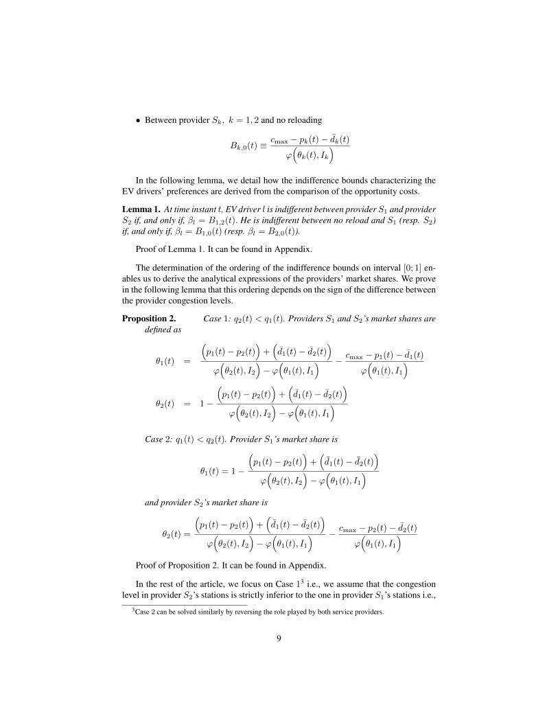
• Between provider Sk, k = 1, 2 and no reloading

Bk,0(t) ≡ cmax − pk(t)− dk(t)

ϕ(θk(t), Ik

)In the following lemma, we detail how the indifference bounds characterizing the

EV drivers’ preferences are derived from the comparison of the opportunity costs.

Lemma 1. At time instant t, EV driver l is indifferent between provider S1 and providerS2 if, and only if, βl = B1,2(t). He is indifferent between no reload and S1 (resp. S2)if, and only if, βl = B1,0(t) (resp. βl = B2,0(t)).

Proof of Lemma 1. It can be found in Appendix.

The determination of the ordering of the indifference bounds on interval [0; 1] en-ables us to derive the analytical expressions of the providers’ market shares. We provein the following lemma that this ordering depends on the sign of the difference betweenthe provider congestion levels.

Proposition 2. Case 1: q2(t) < q1(t). Providers S1 and S2’s market shares aredefined as

θ1(t) =

(p1(t)− p2(t)

)+(d1(t)− d2(t)

)ϕ(θ2(t), I2

)− ϕ

(θ1(t), I1

) − cmax − p1(t)− d1(t)

ϕ(θ1(t), I1

)

θ2(t) = 1−

(p1(t)− p2(t)

)+(d1(t)− d2(t)

)ϕ(θ2(t), I2

)− ϕ

(θ1(t), I1

)Case 2: q1(t) < q2(t). Provider S1’s market share is

θ1(t) = 1−

(p1(t)− p2(t)

)+(d1(t)− d2(t)

)ϕ(θ2(t), I2

)− ϕ

(θ1(t), I1

)and provider S2’s market share is

θ2(t) =

(p1(t)− p2(t)

)+(d1(t)− d2(t)

)ϕ(θ2(t), I2

)− ϕ

(θ1(t), I1

) − cmax − p2(t)− d2(t)

ϕ(θ1(t), I1

)Proof of Proposition 2. It can be found in Appendix.

In the rest of the article, we focus on Case 13 i.e., we assume that the congestionlevel in provider S2’s stations is strictly inferior to the one in provider S1’s stations i.e.,

3Case 2 can be solved similarly by reversing the role played by both service providers.

9

q2(t) < q1(t). This assumption can be justified by assuming that provider S2 investsfar more than S1 in his charging infrastructure i.e., I2 >> I1.

We introduce constraints on the station access prices guaranteeing that both providersmight emerge i.e., that none of them is condemned a priori to have a zero market share.The following lemma is straightforward

Lemma 3. At time instant t, both providers’ prices are chosen so that p2(t)− p1(t) >d1(t)− d2(t), otherwise provider S1 would have a zero market share.

Proof of Lemma 3. It can be found in Appendix.

Suppose that there exists 0 < pmax < +∞ so that at any time, p1(t), p2(t) ≤ pmax.Judging by the providers’ utilities as defined in Equation (1), it is necessary to imposethat p1(t), p2(t) ≥ pE(t) at any time to guarantee the non-negativity of the providers’utilities. Additionally, using Lemma 3, we infer the following price ordering:

pE(t) +(d1(t)− d2(t)

)≤ p1(t) +

(d1(t)− d2(t)

)< p2(t) ≤ pmax (5)

In Proposition 2, θ1(t) (resp. θ2(t)) is still function of θ1(t) and θ2(t) i.e., wehave no simple expression of θ2(t) as a function of θ1(t) solely. However to solve asformally as possible the Stackelberg game described in Section 2, we need to expressθ2(t) as a simple function of θ1(t).

Let

C ≡{

(θ1(t), θ2(t))|θ1(t) + θ2(t) ≤ 1, θ1(t), θ2(t) ∈ [0; 1], ϕ(θ2(t), I2

)< ϕ

(θ1(t), I1

)}be the constraint space containing all the possible market share allocations under theassumption that q2(t) < q1(t) at any time instant t. It is convex as an intersection ofconvex spaces.

The two equations characterizing the providers’ market shares obtained in Propo-sition 2 are recalled below under the constraint that the associated allocations belongto space C

G(1)

θ1(t) = B1,2(t)−B1,0(t)θ2(t) = 1−B1,2(t)(θ1(t), θ2(t)) ∈ C

In order to fix the ideas, we give the mathematical expression of the congestionlevel which is experienced over provider Sk’s charging infrastructure. The chosenmeasure is issued from network optimization literature where the congestion of a linkis traditionally evaluated as a convex latency function of the flow crossing the link[24]. We assume that the congestion level is averaged over all the stations managed bySk and that it is measured as the difference between the market share (θk(t)) and the

10

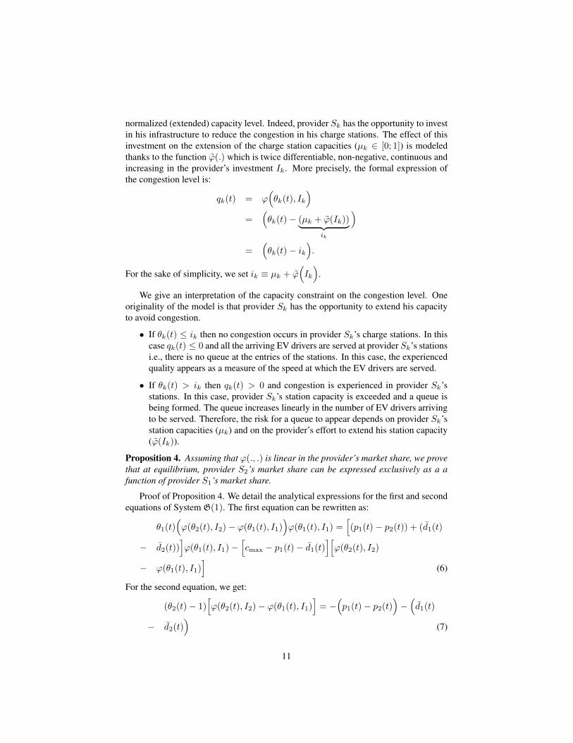
normalized (extended) capacity level. Indeed, provider Sk has the opportunity to investin his infrastructure to reduce the congestion in his charge stations. The effect of thisinvestment on the extension of the charge station capacities (µk ∈ [0; 1]) is modeledthanks to the function ϕ(.) which is twice differentiable, non-negative, continuous andincreasing in the provider’s investment Ik. More precisely, the formal expression ofthe congestion level is:

qk(t) = ϕ(θk(t), Ik

)=

(θk(t)− (µk + ϕ(Ik))︸ ︷︷ ︸

ik

)=

(θk(t)− ik

).

For the sake of simplicity, we set ik ≡ µk + ϕ(Ik

).

We give an interpretation of the capacity constraint on the congestion level. Oneoriginality of the model is that provider Sk has the opportunity to extend his capacityto avoid congestion.

• If θk(t) ≤ ik then no congestion occurs in provider Sk’s charge stations. In thiscase qk(t) ≤ 0 and all the arriving EV drivers are served at provider Sk’s stationsi.e., there is no queue at the entries of the stations. In this case, the experiencedquality appears as a measure of the speed at which the EV drivers are served.

• If θk(t) > ik then qk(t) > 0 and congestion is experienced in provider Sk’sstations. In this case, provider Sk’s station capacity is exceeded and a queue isbeing formed. The queue increases linearly in the number of EV drivers arrivingto be served. Therefore, the risk for a queue to appear depends on provider Sk’sstation capacities (µk) and on the provider’s effort to extend his station capacity(ϕ(Ik)).

Proposition 4. Assuming that ϕ(., .) is linear in the provider’s market share, we provethat at equilibrium, provider S2’s market share can be expressed exclusively as a afunction of provider S1’s market share.

Proof of Proposition 4. We detail the analytical expressions for the first and secondequations of System G(1). The first equation can be rewritten as:

θ1(t)(ϕ(θ2(t), I2)− ϕ(θ1(t), I1)

)ϕ(θ1(t), I1) =

[(p1(t)− p2(t)) + (d1(t)

− d2(t))]ϕ(θ1(t), I1)−

[cmax − p1(t)− d1(t)

][ϕ(θ2(t), I2)

− ϕ(θ1(t), I1)]

(6)

For the second equation, we get:

(θ2(t)− 1)[ϕ(θ2(t), I2)− ϕ(θ1(t), I1)

]= −

(p1(t)− p2(t)

)−(d1(t)

− d2(t))

(7)

11

By substitution of Equation (7) in Equation (6) and by simplification by−(p1(t)−

p2(t))−(d1(t)− d2(t)

), it comes:

ϕ(θ1(t), I1)[θ1(t) + θ2(t)− 1

]+[cmax − p1(t)− d1(t)

]= 0

We then let:

G(θ1(t), θ2(t)) ≡ ϕ(θ1(t), I1)[θ1(t) + θ2(t)− 1

]+[cmax − p1(t)− d1(t)

](8)

Using this simplifying notation, System G(1) becomes:

G(2)

{G(θ1(t), θ2(t)) = 0(θ1(t), θ2(t)) ∈ C

In System G(2) we aim at describing the intersection of the zero-level set of thefunction G(., .) with the constraint space, C. Differentiating G(., .) with respect toθ1(t), we get ∂G(θ1(t),θ2(t))

∂θ1(t) = θ1(t) + θ2(t) − 1. Identically, with respect to θ2(t),

we obtain ∂G(θ1(t),θ2(t))∂θ2(t) = ϕ(θ1(t), I1). Both these differentiates are continuous in

θ1(t) and θ2(t). Using the Implicit function theorem, we know that in cases where∂G(θ1(t),θ2(t))

∂θ2(t) 6= 0 ⇔ θ1(t) 6= i1, there exists a unique function θ2(t) = ψ(θ1(t)),defined and continuous in a neighborhood of θ1(t) ∈ C ∩ {θ1(t) 6= i1} such thatG(θ1(t), ψ(θ1(t))

)= 0.

By substitution ofψ(.) in Equation (8) and using the fact that G(θ1(t), ψ(θ1(t))

)=

0, we obtain the analytic expression of function ψ(.) which enables us to express θ2(t)as a function of θ1(t) solely, i.e.:

θ2(t) = ψ(θ1(t)

)=

(1− θ1(t)

)+p1(t) + d1(t)− cmax

θ1(t)− i1.

System G(2) can then be rewritten by expliciting θ2(t) as a function of θ1(t) exclu-sively. It gives us a new system of equations that we call G(3).

G(3)

θ2(t) = ψ

(θ1(t)

)= (1− θ1(t)) + p1(t)+d1(t)−cmax

θ1(t)−κ1

(θ1(t), θ2(t)) ∈ C

The solutions of System G(3) (provided they exist) are contained in the solutions ofSystem G(1). Furthermore, if we impose the additional constraint that θ1(t) + θ2(t) =x for any 0 < x < 1 in System G(3), then making x vary enables to browse all thesolutions of System G(1).

12

3.2 Optimal pricingIn this section, we solve step (2) of the repeated Stackelberg game described in Sec-tion 2. As usual in multi-level games, we proceed by backward induction [3], [15].Step (3) has already been solved in Section 3.1: the EV drivers allocation between theservice providers are obtained through System G(3) which relies on service providerS1’s price p1(t). Going to step (2), we want to determine the prices p1(t), p2(t) max-imizing the providers’ utilities as defined in Equation (1) and taking into account theprice constraint defined in Equation (5).

The price ordering obtained in Equation (5) can be decomposed into the followingconstraints, giving intervals of definition for both service providers’ prices:

• pE(t) ≤ p1(t) < p2(t)−(d1(t)− d2(t)

)for provider S1,

• p1(t) +(d1(t)− d2(t)

)< p2(t) ≤ pmax for provider S2.

The utilities defined in Equation (1) being continuous, the service providers’ opti-mal prices are reached either in their interior or at one boundary of their price interval ofdefinition. Besides, System G(3) depends only on service provider S1’s price which inturn, affects provider S2’s pricing strategy since the upper bound of provider S2’s priceinterval of definition depends on p1(t). Depending on whether the optimal prices arereached at the interior or at one boundary of the interval of definition, 4 cases emerge.They are detailed below.

3.2.1 Case 1: The service providers’ optimal prices are reached in the interiorof their price intervals of definition

It means that p1(t) ∈]pE(t); p2(t) − (d1(t) − d2(t))[ and p2(t) ∈]p1(t) + (d1(t) −d2(t)); pmax[. At the equilibrium, for any k = 1, 2, provider Sk’s utility should besolution of the following equation: ∂πk(t)

∂pk(t) = 0. Then, for any provider Sk, k = 1, 2,we have the following equivalences:

∂πk(t)

∂pk(t)= 0 ⇔ θk(t) + (pk(t)− pE(t))

∂θk(t)

∂pk(t)= 0

⇔ ∂θk(t)

θk(t)= − ∂pk(t)

pk(t)− pE(t)

⇔ log(θk(t)) = log(1

pk(t)− pE(t))

⇔ θk(t) =1

pk(t)− pE(t)since log is a bijective function.

We infer that pk(t) = pE(t) + 1θk(t) for any provider Sk, k = 1, 2 and by substitu-

tion in System G(3), we obtain a new system of equations:

13

G(3, 1)

θ2(t) = ψ(θ1(t))

=(

1− θ1(t))

+ 1θ1(t)−i1

[pE(t) + 1

θ1(t) + d1(t)− cmax

](θ1(t), θ2(t)) ∈ C

The objective is now to prove the existence and unicity of solutions for System G(3, 1).

Unicity of solution for System G(3, 1). In the following lemma, we prove theunicity of System G(3, 1) solution for any value of the total market share4 x ∈ [0; 1]such that θ1(t) + θ2(t) = x.

Lemma 5. For any x ∈ [0; 1] there exists a unique couple of value (θ1(t), θ2(t)) suchthat θ1(t) + θ2(t) = x and θ2(t) = ψ(θ1(t)).

Proof of Lemma 5. It can be found in Appendix.

Although we have proved that ψ(.) is increasing over interval [0; 1], we have noguarantees about its concavity yet. Indeed it might admit an inflection point over theinterval. In the following lemma, we introduce a sufficient condition on cmax, the EVdrivers’ maximum admissible opportunity cost, guaranteeing the concavity of functionψ(.) over interval [0; 1].

Lemma 6. If cmax ≤ (1− i1) + pE(t) + d1(t) then ψ(.) is concave in θ1(t).

Proof of Lemma 6. It can be found in Appendix.

Existence of solution for System G(3, 1). In the following proposition, we detailconditions on i1, i2 guaranteeing the existence of solutions for System G(3, 1), for anyfixed value of the total market share x ∈ [0; 1] such that θ1(t) + θ2(t) = x.

We introduce two three-order polynoms that will be useful in the following propo-sition proof:

P1

(θ1(t)

)≡ 2θ3

1(t)− θ21(t)

[1 + 2i1 +

(ϕ(I1)− ϕ(I2)

)]− θ1(t)

[− i1

(1

+ (ϕ(I1)− ϕ(I2)))

+ pE(t) + d1(t)− cmax

]− 1

and

P2

(θ1(t)

)≡ θ3

1(t)− θ21(t)(1 + i1) + θ1(t)

(κ1 − pE(t)− d1(t) + cmax

)− 1

The limits in −∞ and +∞ of P1(.) (resp. P2(.)) being infinite and of oppositesigns, function P1(.) (resp. P2(.)) being continuous since polynomial, the intermediatevalue theorem provides us the guarantee of the existence of at least a real root solutionof the equation: P1(.) = 0 (resp. P2(.) = 0). The three roots associated with polynomP1(.) are denoted rP1(l), l = 1, 2, 3 (resp. rP2(l), l = 1, 2, 3 for polynom P2(.)).

4In economics, the total market share i.e., the sum of the rival providers’ market share is also calledpenetration or market coverage rate [13].

14

We give necessary and sufficient conditions on i1, i2 guaranteeing that System G(3, 1)admits a solution.

Proposition 7. Suppose providers S1 and S2’s optimal prices are reached in the inte-rior of their price intervals of definition.

• In case where θ1(t) < i1 (no congestion), System G(3, 1) admits a solution if,and only if, i1, i2 are chosen so that

i1 ≤1

cmax − d1(t)− pE(t)

θ1(t) ∈ [0; rP1(1)[ ∪ ]rP1

(1); rP1(3)[

θ1(t) ∈ [rP2(1); rP2

(2)] ∪ [rP2(3); +∞[

θ1(t) ∈ [0; 1]

• In case where θ1(t) ≥ i1 (congestion occurs), System G(3, 1) admits a solutionif, and only if, i1, i2 are chosen so that

i1 >1

cmax − pE(t)− d1(t)

θ1(t) ∈ [rP1(1); rP1

(2)] ∪ [rP1(3); +∞[

θ1(t) ∈ [0; rP2(1)[ ∪ ]rP2

(2); rP2(3)[

θ1(t) ∈ [0; 1]

Proof of Proposition 7. It can be found in Appendix.

As a corollary of Proposition 7, if we impose that the whole market is captured i.e.,θ1(t) + θ2(t) = 1 then the EV driver allocation is unique: θ1(t) = 1

cmax−pE(t)−d1(t)

and θ2(t) = 1− θ1(t). In all generalities, if we fix the number of EV drivers delayingtheir reload as 1 − x ∈]0; 1] then the optimal number of consumers for provider S1

satisfying θ1(t) + θ2(t) = x is defined uniquely as:

θ1(t) =1

2

( 1

x− 1(pE(t) + d1(t)− cmax) + i1

−

√(

1

1− x(pE(t) + d1(t)− cmax) + i1)2 +

4

1− pE(t)

).

Then θ2(t) is inferred from the relation: θ2(t) = x− θ1(t).

3.2.2 Case 2: Provider S1’s optimal price is reached at the inferior bound of hisprice interval of definition.

In this case, p1(t) = pE(t) and pE(t) + (d1(t)− d2(t)) < p2(t) ≤ pmax. By substitu-tion of provider S1’s optimal price in System G(3), we obtain:

G(3, 2)

θ2(t) = ψ(θ1(t))

= (1− θ1(t)) + 1θ1(t)−i1

[pE(t) + d1(t)− cmax

](θ1(t), θ2(t)) ∈ C

(9)

15

Proposition 8. Suppose provider S1’s optimal price is reached at the inferior boundof his price interval of definition. System G(3, 2) admits a unique solution θ1(t) = 0and θ2(t) = 1− 1

i1[pE(t) + d1(t)− cmax] if, and only if, cmax ≤ pE(t) + d1(t).

Proof of Proposition 8. It can be found in Appendix.

As a corollary of Proposition 8, the whole market is captured by provider S2 if, andonly if, cmax = pE(t) + d1(t). In all the other cases, it is impossible for the providerto capture the total market.

3.2.3 Case 3: Provider S1’s optimal price is reached at the upper bound of hisprice interval of definition and provider S2 in the interior of his price in-terval of definition

Under these assumptions, there exists a real ε > 0 such that ε→ 0 and p1(t) = p2(t)−(d1(t)− d2(t))− ε. Provider S2 price constraint becomes: p1(t) + (d1(t)− d2(t)) <p2(t) ≤ pmax. Since S2 reaches his optimal price in the interior of the interval, wehave: p2(t) = pE(t) + 1

θ2(t) .

Proposition 9. Suppose provider S1’s optimal price is reached at the upper bound ofhis price interval of definition and provider S2 in the interior of his price interval ofdefinition. The relations between the providers’ market shares take the following formsdepending whether congestion occurs.

• If θ1(t) > i1 (congestion occurs),

θ2(t) =1

2

[(1− θ1(t)) +

1

θ1(t)− i1(pE(t) + d1(t)− cmax)

+

√[(θ1(t)− 1)− 1

θ1(t)− i1(pE(t) + d1(t)− cmax)]2 +

4

θ1(t)− i1

].

• If θ1(t) ≤ i1 (no congestion),

θ2(t) =1

2

[(1− θ1(t)) +

1

θ1(t)− i1(pE(t) + d1(t)− cmax)

−

√[(θ1(t)− 1)− 1

θ1(t)− i1(pE(t) + d1(t)− cmax)]2 +

4

θ1(t)− i1

].

Proof of Proposition 9. It can be found in Appendix.

As a corollary of Proposition 9, if we assume that the whole market is capturedwe infer each provider’s market share: θ2(t) = 1

(ε+cmax)−(d2(t)+pE(t))and θ1(t) =

1− θ2(t).

16

3.2.4 Case 4: Both providers reach their optimal prices at the upper bounds oftheir own price interval of definition

It means that p2(t) = pmax from which we infer p1(t) = pmax − (d1(t)− d2(t))− ε.

Proposition 10. Suppose that both providers reach their optimal prices at the upperbounds of their own price interval of definition, the relation between the providers’market shares takes the following form:

θ2(t) = (1− θ1(t)) +pmax − ε+ (d2(t)− cmax)

θ1(t)− i1

Proof of Proposition 10. It is straightforward by substitution of provider S1’s opti-mal price in the equation: θ2(t) = ψ(θ1(t)) described in System G(3).

As a corollary of Proposition 10, if we assume that the whole market is captured,we infer that: cmax = pmax − ε+ d2(t). This means that no EV drivers would chooseprovider S2. Therefore, θ1(t) = 1 and θ2(t) = 0.

4 Optimization of the charging infrastructure topolo-gies using the Cross-Entropy method

In this section, the service providers determine simultaneously and independently thenumber of stations that they wish to settle as well as their locations on the R2 plane.This coincides with step (1) of the game described in Section 2. Step (1) is solved soas to optimize the service provider’s utility over the complete duration of the game i.e.,over time interval [0;T ]. For this purpose, we need to define service provider Sk, k =1, 2’s long-term utility. Indeed, in general, the optimal decisions of a player differin cases where we consider a repeated game that leads to a sequencial optimizationproblem and in cases where the decisions are optimized over the entire course of thegame. In our game setting, provider Sk, k = 1, 2 chooses Nk ∈ N∗ as the numberof stations to settle and sk ∈ R2Nk , k = 1, 2 as their locations on the R2 plane. Hislong-term utility is the sum of his one-shot utilities as described in Equation (1) whichoutputs are added sequentially over the discretized finite horizon [0;T ], coefficientedby a discount factor δ ∈]0; 1]5:

Πk(s1, s2) =

T∑t=0

δtπk(t) (10)

x ∈ [0; 1] is the total market share i.e., the sum of both providers’ market shares.It is known publicly by all the providers and satisfies: θ1(t) + θ2(t) = x at any time

5The discount factor is supposed identical for both providers. It means that both of them has the samerisk aversion level for the future [28], [34]. The introduction of a discount factor is classical in (stochastic)dynamic programming and repeated game theory where the players consider their long-term utilities andhave uncertainties on the future. However, extensions where it differs between the rival providers could beconsidered in a companion paper more devoted to simulation results.

17

instant t. It is supposed constant over time since the batteries have a limited autonomywhich force the EV drivers to reload periodically in time. Using the total market sharevalue, Cases 1, 2 and 4 as described in Section 3.2, can be solved analytically. Inthese cases, the resolution of the pricing game requires to solve polynomial equationsin the market shares. Case 3 is more complex and requires a numerical resolution toidentify the service providers’ market shares. However, in all the cases, it is impossibleto determine analytically the service providers’ optimal number of stations as wellas their locations, since the EV drivers’ choices depend on their spatial distributionon the plane which is modeled as a time-dependent density function in Equation (3).Consequentely, we resort to use simulation to determine the optimal topologies of theservice providers’ charging infrastructures.

We decouple the problem of determining the optimal number of stations to settle inthe R2 plane which is solved numerically from the problem of optimizing the stationlocations on the R2 plane which is solved through simulation. We now describe bothphases. For any service provider Sk, k = 1, 2, the problem of optimizing his charginginfrastructure topology can be written as:

γ∗k = Πk(s∗1, s∗2) = max

sk∈R2Nk

Πk(sk, s∗{1,2}−k) (11)

where s∗{1,2}−k denotes the vector containing the station locations of the provider dif-ferent from Sk for k = 1, 2, γ∗k is the maximum long-term utility output for serviceprovider Sk. It is not necessarily unique and might be different for the rival providers.

To determine the charging infrastructure topologies optimizing Equation (11), wetransform the initial deterministic optimization problem in an estimation one. Thecross-entropy method introduced by Rubinstein et al. [8], [27] is a general Monte-Carlo approach to combinatorial problems like the travelling salesman, quadratic as-signment, etc., continuous multi-extremal optimization and importance sampling [11].It originates from the field of rare event simulation where very small probabilities needto be accurately estimated like in queueing theory applications or more generally, per-formance analysis of complex systems. The method has been successfully applied toproblems belonging to the field of combinatorial optimization [12] which are consid-ered to be hard to solve. There have been many successful applications of the methodto diverse fields such as routing and performance evaluation in telecommunication net-works [27], queueing theory, sensor selection/management [31], the optimization ofthe locations of a sparse antenna array [20], etc. Le Cadre et al. use it to solve theglobal level when decomposing a hierarchical search problem in two optimization lev-els. They check that it enables to find optimal solutions in most cases with a reasonabletime [31]. These points motivated us in our turn to use the method. Additionally, weobtain as output of the algorithm the optimal density function generating the chargestation locations which is quite original compared to previous approaches in combi-natorial optimization [5] and might facilitate potential computations of performancemeasures.

To apply the cross-entropy method to our problem, we need to suppose that providerSk, k = 1, 2 station locations are distributed according to a density parametrized by a

18

multi-dimensional vector of parameters called ρk, k = 1, 2 i.e.,sk = (sk(1), ..., sk(Nk)) ∼ f(., ρk) where ρk ∈ R2Nk . We let γk be a fixed level forservice provider Sk’s long-term utility. For a certain ρk ∈ R2Nk , we associate with(11), the problem of estimating the number l(γk):

l(γk) = Pρk [Πk(s, s∗{1,2}−k) ≥ γk] =

∫s∈R2Nk

1{Πk(s,s∗{1,2}−k)≥γk}f(s, ρk)ds

= Eρk [1{Πk(s,s∗{1,2}−k)≥γk}] (12)

We give below a description of the algorithm that we use to optimize the serviceproviders’ charging infrastructure topologies. It is based on updates of density param-eters ρk ∈ R2Nk , k = 1, 2.

4.1 Algorithm descriptionWe take service provider Sk, k = 1, 2’s point of view. The algorithm is based on thecross-entropy method introduced by Rubinstein et al. in [8], [27]. We use the followingconvention: for any real number r ∈ R, dre corresponds to the smallest integer numbersuperior to r.

Algorithm: Charging infrastructure topology optimization

Parameters:

• M ∈ N∗ number of iterations

• Ns ∈ N∗ sample size

• ζ ∈]0; 1[ one minus the value of the quantile associated to the performance statis-tics

• d ∈ N∗ stopping criterion

The algorithm is run for m = 1, ...,M iterations.

1. Define ρk(0). Set m = 1.

2. For any m ∈ {1, ...,M}. Generate a sample (s1k, ..., s

Ns

k ) ∼ f(., ρk(m − 1))

where slk ∈ R2Nk , ∀l = 1, ...,Ns. Let Π1k = Πk(s1

k, s∗{1,2}−k),..., ΠNs

k =

Πk(sNs

k , s∗{1,2}−k) and determine the associated ordered statistic: Π(1)k ≤ ... ≤

Π(Ns)k . Compute the (1 − ζ) quantile γk(m) of the performance according to

γk(m) = Πk(d(1− ζ)Nse).

3. Use the same sample s1k, ..., s

Ns

k and solve:

ρk(m) = maxρk∈R2Nk

1

Ns

Ns∑l=1

1Πk(slk,s∗{1,2}−k

)≥γk(m)logf(slk, ρk) (13)

19

4. If for some m ≥ d (ex.: d = 5), ρk(m) = ρk(m − 1) = ... = ρk(m − d) thenstop. Otherwise set m = m+ 1 and go back to step 2 of the algorithm.

Making some assumptions on the station location generating density, we now detailhow to solve Equation (13).

For the sake of simplicity, service provider Sk’s l-th station coordinates are storedin the two-dimensional coordinate vector:

sk(l) = (sk(l)|x, sk(l)|y) ∈ R2

where sk(l)|x contains vector sk(l) projection on the x-axis and sk(l)|y , on the y-axis.We assume that there exists a bijective mapping between the station coordinates

and the first 2Nk integers:

M : sk(1)|x, sk(1)|y, ..., sk(Nk)|x, sk(Nk)|y 7→ {1, 2, ..., 2Nk − 1, 2Nk}

Practically, this means that two charge stations settled by provider Sk cannot shareidentical x-axis (resp. y-axis) coordinates. Using the same idea, for any generatedsample l = 1, ...,Ns, there exists a bijective application Ml(.), mapping the l-th coor-dinate vector slk on the first 2Nk integers:

Ml : slk(1)|x, slk(1)|y, ..., slk(Nk)|x, slk(Nk)|y 7→ {1, 2, ..., 2Nk − 1, 2Nk}

Besides, we assume that at iteration step m ∈ {1, ...,M} of the algorithm, serviceprovider Sk’s station locations are distributed according to a 2Nk- dimensional normaldensity with covariance matrix:

σk =

σk(1, 1) . . . σk(1, 2Nk)...

......

σk(2Nk, 1) . . . σk(2Nk, 2Nk)

. The covariance matrix contains

the uncertainty levels associated with the knowledge of the service providers’ stationlocations. It is supposed fixed a priori and known publicly. We make the assump-tion that the covariance matrix coefficients remaining on its diagonal always remainpositive. They coincide with the variances associated with provider Sk’s stations coor-dinates.

The mean ρk(m) ∈ R2Nk associated with the 2Nk-components of the normal den-sity are unknown and should be estimated through Equation (13) solving. Differentiat-ing Equation (13) with respect to the mean components, we obtain that it is equivalentto solve the following matricial system:

ρk(m) =1∑N

l=1 1Πk(slk,s∗{i,j}−k

)≥γk(m)

N∑l=1

1Πk(slk,s∗{i,j}−k

)≥γk(m)R−1k Clk

20

whereClk =

slk(1)|x+ 12

∑h6=1

σk(1,h)σk(1,1)M

l,−1(h)

slk(1)|y + 12

∑h6=2

σk(2,h)σk(2,2)M

l,−1(h)...

slk(Nk)|x+ 12

∑h6=2Nk−1

σk(2Nk−1,h)σk(2Nk−1,2Nk−1)M

l,−1(h)

slk(Nk)|y + 12

∑h6=2Nk

σk(2Nk,h)σk(2Nk,2Nk)M

l,−1(h)

and Ml,−1(.)

denotes the inverse of mapping Ml(.) associated with the l-th generated sequence.

Rk is a 2Nk × 2Nk matrix defined so that Rk(i, i) = 1, ∀i = 1, ..., 2Nk andRk(j, i) = 1

2σk(j,i)σk(j,j) ≥ 0, ∀i, j = 1, ..., 2Nk, i 6= j. Note that using the co-

variance definition, Rk is semi-positive definite and we observe that: Rk(j, i) =Rk(i, j), ∀i, j = 1, ..., 2Nk, i 6= j. This last point implies that matrix Rk is sym-metric.

Lemma 11. Matrix Rk is invertible.

Proof of Lemma 11. It is trivial to check that Rk is invertible. Using the covariancedefinition, we have the inequality:

1 0 . . . 00 1 . . . 0...

. . . . . ....

0 0 . . . 1

≤ Rkwhere inequality between two matrices of the same size is defined coordinate per co-ordinate. Determinant being a linear form, we infer that: 1 ≤ det(Rk).

The results obtained above are summarized in the following theorem.

Theorem 12. Assuming that service provider Sk’s stations locations are distributedaccording to a 2Nk- dimensional normal density centered in vector ρk(m) and of fixedcovariance matrix σk, the updating rule of vector ρk(m) as described in Equation (13)is equivalent with the matricial equation:

ρk(m) =1∑Ns

l=1 1Πk(slk,s∗{1,2}−k

)≥γk(m)

Ns∑l=1

1Πk(slk,s∗{1,2}−k

)≥γk(m)R−1k Clk

where Clk =

slk(1)|x+ 12

∑j 6=1

σk(1,j)σk(1,1)M

l,−1(j)

slk(1)|y + 12

∑j 6=2

σk(2,j)σk(2,2)M

l,−1(j)...

slk(Nk)|x+ 12

∑j 6=2Nk−1

σk(2Nk−1,h)σk(2Nk−1,2Nk−1)M

l,−1(j)

slk(Nk)|y + 12

∑j 6=2Nk

σk(2Nk,j)σk(2Nk,2Nk)M

l,−1(j)

and Rk is a

symmetric invertible 2Nk × 2Nk matrix defined so that Rk(j, j) = 1, ∀j = 1, ..., 2Nkand Rk(i, j) = 1

2σk(i,j)σk(i,i) ≥ 0, ∀i, j = 1, ..., 2Nk, i 6= j.

21

Figure 1: Cone of the simulated EV trajectories.

5 Numerical illustrationsThe aim of this section is to explain practical realisations of the model elaborated inthis article and to provide some economic guidelines.

The total number of EV on the market is supposed constant: N = 100. How-ever, the number of EVs which reload at each time instant t is defined as a fractionof the total number of EVs i.e., there exists a random variable α(t) ∈ [0; 1] such thatN(t) = α(t)N . In the numerical analysis, we assume that α(t) is generated accordingto the uniform density over interval [0; 1]. Additionally, the EV drivers’ trajectories aregenerated according to independent two-dimensional brownian motions whose com-ponents are correlated. N independent brownian motions are generated. To generateN correlated brownian motions, we need to specify the correlation matrix between thecomponents of these brownian motions: Q, which is of size N ×N . At time instant t,the matrix containing the variances-covariances of the N correlated Brownian motionequals: Q(t) = tQ. Then, the Choleski decomposition of matrix Q(t) enables us toexpress the correlated brownian motion components as a linear combination of the Nindependent brownian motions.

The mean value of the distance between the EV drivers and provider Sk, k = 1, 2is obtained as an approximation of Equation (3). At each time instant t, once theEV locations on the R2 plane has been obtained through the realizations of the N(t)correlated brownians motions, for each provider Sk, we compute the minimum of theirdistance to the closest station of the provider and average this value over N(t).

As an illustration, in Figure 1, we have simulated the trajectories of 4 EVs startingfrom the same origin (0; 0), over time interval [0; 100]. The cone of the 100 simulatedtrajectories for the EVs is represented in light blue.

In all this section, the game parameters are fixed as follows:

• The discount factor is: δ = 0.7.

• The service providers’ capacity per station are: µ1 = 0.83, µ2 = 0.90.

22

• The providers’ investment level increases linearly in the number of stations set-tled i.e.: I1 = 0.01N1 + 0.05 and I2 = 0.03N2 + 0.02.

• Provider Sk, k = 1, 2’s extended capacity is defined as: ik = µk + 0.1Ik.

• The total market share also called market coverage in the article, is: x = 0.8.

• The repeated pricing game parameters are defined as: T = 100, pmax = 50,cmax = 100, pE = 10, cE = 10, ε = 10−3.

• σ1 and σ2 are non-negative symmetric matrices whose upper-diagonal and di-agonal coefficients are generated according to a uniform density on interval[10−3; 1].

• For the cross-entropy algorithm, the sample size is fixed so that: Ns = 10 and theassociated quantile is: ζ = 0.7. Finally, the cross-entropy algorithm maximumnumber of iterations is: M = 100.

5.1 Optimization of the charging infrastructure topologiesEach provider can settle: 5, 15 or 25 stations over the R2 plane. This gives rise to 32

potential combinations. The long-term utilities of both providers are stored in Table 1below, for each potential combination of numbers of stations.

PPPPPPPPN1

N2 5 15 25

5 (−23.38; 204.97) (−97.55; 333.67) (443.93;962.40)15 (649.97;−23.04) (−57.65; 691.24) (510.34; 601.63)25 (895.43;231.71) (64.62;−319.58) (−21.55;−531.99)

Table 1: Providers’ long-term utilities as functions of the number of settled stations.

We observe that there are two pure Nash equilibria (NE) in Table 1. They are bothhighlighted in bold and correspond to the cases: N1 = 5, N2 = 25 for the first NEand N1 = 25, N2 = 5 for the second one. NE N1 = 5, N2 = 25 is more favorable toprovider S2 who maximizes his long-term utility over all the potential combinations ofnumber of stations whereas NE N1 = 25, N2 = 5 is more favorable to provider S1. Asa result, the system might become instable if the providers does not agree and generateperiodic go-backs between the two NEs. However, if it is an unbiased decision makerwho drives the system, he will force the system to stabilize in the first NE. Indeed, thislatter coincides with the game maximum social welfare i.e., it maximizes the sum ofboth providers’ long-term utilities.

In Figure 2, we have represented the providers’ long-term utilities obtained as out-put of the dynamic pricing game, as functions of the number of stations settled by eachprovider. The two NEs are highlighted by squares.

23

Figure 2: Numerical determination of the number of stations to settle.

Figure 3: Providers’ long-term utilities as functions of their market share.

5.2 Market coverageIn Figure 3, we have represented the logarithm of both providers’ long-term utilities(provider S1 in blue with o and provider S2 in magenta with ∗) as functions of themarket coverage called x ∈ [0; 1] in all the article. We observe that provider S1’s long-term utility is increasing provided 0 ≤ x ≤ 0.6 whereas provider S2’s long-term utilityis increasing provided 0.8 ≤ x ≤ 1. This enables us to define intervals for x, the firstone being favorable to S2 and the second one to S1. The value x = 0.8 appears asgood compromise since it is not penalizing any of the providers.

5.3 An alliance to share the investments in the charging infrastruc-ture?

Sorensen indexes are traditionally used in ecology to characterize the similarity interms of species present on two geographic area [2]. We make the analogy with ourillustration by defining 4 species: none of the providers (spece 0); provider S1 exclu-sively (spece 1); provider S2 exclusively (spece 2); both providers (spece 3). To definegeographic areas, we realize a mesh over the R2 plane. It is delimitated by the extremecoordinates of the settled stations:

24

Figure 4: Density of the station locations.

[mink=1,2{minl=1,...,Nk

sk(l)|x}; maxk=1,2{maxl=1,...,Nksk(l)|x}

]×[

mink=1,2{minl=1,...,Nksk(l)|y}; maxk=1,2{maxl=1,...,Nk

sk(l)|y}]. It is then divided

into a collection of squares of equal size. Over each axis, the division step is fixed at100 giving rise to 1002 squares of equal size.

In top of Figure 4, we have plotted the optimal stations locations over the R2 planefor the first NE (N1 = 5, N2 = 25) at left and for the second NE (N1 = 25, N2 = 5) atright. At the bottom of the figure, we have represented the number of species rankingfrom 0 to 3 present in each square of the mesh area. In case of the first NE, the sta-tion locations are complementary i.e., each provider covers a closed area of the planeand the intersection between both coverage area is negligeable. In case of the secondNE, the stations are more densely concentrated and there appears a conflict in the lo-cations. The complementary configuration seems more promising since it generateshigher long-term utilities than the conflicting one as observed in Section 5.1. Addition-ally, it might favor the emergence of geographic alliances between the providers en-abling them to share their charging infrastructure investment cost while widening theircoverage area. Mechanisms of cost sharing between the involved providers should thenbe designed so as to encourage long-term collaboration between them. This is one ofthe subject extensively studied in the mechanism design theory [21], [29]. It mightprovide possible extensions of this article.

6 ConclusionIn this article, we have considered two competitive service providers optimizing inde-pendently and simulatneously their charging infrastructure topology (in number of sta-tions managed and in locations) while dynamically updating their station access pricesso as to maximize their utility. The resulting two-stage game is solved in two steps.

25

First, the pricing game is solved using backward induction. We characterize analyti-cally the unique Nash equilibrium in prices, at each time instant. Then, the chargininginfrastructure is optimized using simulation to determine the station locations and nu-merical analysis to optimize their number.

Interesting extensions of the article might generalize the two-stage game resolutionto an arbitrary large number of interacting service providers. In this case, the analyticapproach provided in this article to solve the pricing game does not hold anymore. Afirst alternative might be to model the game as a differential one and to determine theoptimal open-loop strategies in prices for the service providers [6]. A second alternativemight be to consider the game as a cooperative one where coalitions might emerge[3], [21]. In such a case, the prices might be optimized using a convenient sharingmechanism for the coalitions. Another possible extension should be to add a third levelto the two-stage game, by assuming that the energy provider M makes his price varydynamically and that the energy that he can sold to the service providers at any timeinstant is constrained by his network capacity.

Appendix

Proof of Lemma 1As stated above, EV driver l is indifferent between S1 and S2 if, and only if, cl(1, t) =

cl(2, t) ⇔ βl =

(p1(t)−p2(t)

)+

(d1(t)−d2(t)

)ϕ

(θ2(t),I2

)−ϕ(θ1(t),I1

) . Identically, EV driver l is indifferent

between Sk and no reload if, and only if, cl(k, t) = cmax ⇔ βl = cmax−pk(t)−dk(t)

ϕ

(θk(t),Ik

) ,

for any k = 1, 2.

Proof of Proposition 2To determine which provider is preferred at the left or at the right of the indifferencebound B1,2(t), it is important to determine the relative order between q1(t) and q2(t).Let consider an arbitrar EV driver l.

Suppose for instance that q2(t) < q1(t) then cl(1, t) < cl(2, t) i.e., provider S1 ispreferred over provider S2 if, and only if, βl < B1,2(t). This case is denoted Case 1.

But, if q1(t) < q2(t) then cl(1, t) < cl(2, t) i.e., provider S1 is preferred overprovider S2 if, and only if, B1,2(t) < βl. This case is denoted Case 2.

Depending on the EV drivers’ congestion sensitivity coefficient position on interval[0; 1], it is possible to determine the providers’ market shares since the EV drivers’sensitivity coefficient is supposed to be distributed according to the uniform density onthe interval [0; 1] by the assumption described in Section 2. We obtain the followingmarket shares:

In Case 1, θ2(t) = 1−B1,2(t), θ1(t) = B1,2(t)−B1,0(t).

26

In Case 2, θ1(t) = 1−B1,2(t), θ2(t) = B1,2(t)−B2,0(t).

Informally, it is possible to interpret the EV drivers choices with the following ar-guments: When the EV drivers congestion sensitivity coefficient approaches 1, theychoose the provider offering the smallest congestion level. When their sensitivity co-efficient takes intermediate values, they might be less sensitive to the congestion thanto the price. As a result, in this case, they accept to reload in the stations of the serviceprovider having the highest congestion level. Finally, when their sensitivity coefficientapproaches 0, the EV drivers are rather insensitive to the congestion i.e., they are notso eager to reload and can delay it.

Proof of Lemma 3By assumption, the congestion level in S2’s charge stations is smaller that in S1’s onessince we have supposed that q2(t) < q1(t). At time instant t, provider S2 is alwayspreferred over provider S1 by any EV driver l if, and only if, cl(2, t) ≤ cl(1, t) ⇔p2(t) + βlq2(t) + d2(t) ≤ p1(t) + βlq1(t) + d1(t) ⇔ p2(t) − p1(t) ≤ d1(t) − d2(t)

since βl(q1(t)− q2(t)

)> 0 by assumption.

Proof of Lemma 5Differentiating ψ(.) once with respect to θ1(t), we obtain:ψ′(θ1(t)) = −1 − 1

(θ1(t)−i1)2 (pE(t) + 1θ1(t) + d1(t) − cmax) − 1

θ1(t)−i11

θ21(t). By

absurd reasoning, we assume that ψ′(θ1(t)) < 0. This is equivalent with the follow-ing inequality: − 1

(θ1(t)−κ1)2 (pE(t) + 1θ1(t) + d1(t) − cmax) + 1

θ1(t)−i1 (− 1θ21(t)

) < 1.

Multyplying each side of the inequality by the term (θ1(t) − i1)2θ1(t), we infer:θ4

1(t)− 2i1θ31(t) + θ2

1(t)[i21 − d1(t) + cmax − pE(t)]− i1 > 0. This inequality shouldbe true for any θ1(t) ∈ [0; 1]. But at the boundary θ1(t) = 0 we obtain −i1 > 0which contradicts the definition of i1 given in Section 3.1. Therefore, ψ′(.) is positiveover interval [0; 1] meaning that function ψ(.) is increasing other this interval. As a byproduct, the intersection of function ψ(.) with the line of equation θ2(t) = x− θ1(t) isunique.

Proof of Lemma 6Differentiating ψ(.) twice with respect to θ1(t), we obtain:

ψ′′(θ1(t)) =2(pE(t) + 1

θ1(t) + d1(t)− cmax)

(θ1(t)− i1)3+

2

θ31(t)(θ1(t)− i1)

+2

θ21(t)(θ1(t)− i1)2

From this, we infer that ψ(.) cannot be convex provided it is continuous by assumption.Reducing ψ′′(.) to the same denominator θ3

1(t)(θ1(t) − i1)3, we obtain ψ′′(.) < 0 ⇔

27

θ31(t)(pE(t)+d1(t)−cmax)+θ1(t)(3θ1(t)−2i1)+2κ2

1 < 0. This is a polynom of order3 in θ1(t). The constant coefficient is positive whereas the coefficient of the higest orderterm (pE(t) + d1(t) + cmax) is negative. Indeed, if it were non-negative, provider S1

would not have any clients. Besides, the polynom derivative is negative in zero meaningthat the polynom is decreasing in the neighborhood of zero. As a result, if the polynomadmits three real roots, there are necessarily non-negative. The polynom admits aunique minimum and a unique maximum. A sufficient condition to guaranteeing thatθ3

1(t)(pE(t) + d1(t) − cmax) + θ1(t)(3θ1(t) − 2i1) + 2i21 < 0 is to impose that thegame parameters are chosen so that the polynom minimum is greater than 1. But, the

polynom minimum is reached in 6+√

36+24(pE(t)+d1(t)−cmax)κ1

6(cmax−pE(t)+d1(t)). Finally, this value is

smaller than 1 if, and only if, cmax ≤ (1− i1) + pE(t) + d1(t).

Proof of Proposition 7ψ(.) being increasing (cf. Lemma 5), System G(3, 1) admits a solution if, and only ifthe couple of allocations (θ1(t), θ2(t)) belongs to the constraint space C. Formally, itmeans that the following inequalities should be simultaneously checked:

0 ≤ θ1(t) ≤ 1 (14)ψ(θ1(t)) ≤ 1− θ1(t) (15)

ψ(θ1(t)) ≤ θ1(t)−(ϕ(I1)− ϕ(I2)

)(16)

ψ(θ1(t)) ≥ 0 (17)

Constraint (15) gives us 1θ1(t)−i1 [pE(t) + 1

θ1(t) + d1(t)− cmax] ≤ 0. Depending onthe sign of θ1(t) − i1, two cases appear. Either θ1(t) < i1 i.e., there is no congestionin provider S1’s stations, or θ1(t) ≥ i1 i.e., congestion occurs. It is easy to check thatif θ1(t) < i1, the second constraint is checked if, and only if, i1 ≤ 1

cmax−d1(t)−pE(t).

If θ1(t) ≥ i1; the second constraint is checked if, and only if, i1 > 1cmax−pE(t)−d1(t)

.

Constraint (16) is equivalent with (1 − θ1(t)) + 1θ1(t)−i1 [pE(t) + 1

θ1(t) + d1(t) −

cmax] ≤ θ1(t)−(ϕ(I1)− ϕ(I2)

). To simplify the expression, we need to multiply it

by (θ1(t)− i1)θ1(t). The two cases cited above already hold.Besides, we note that P1(0) = −1 < 0 and that P ′1(0) = i1(1+

(ϕ(I1)−ϕ(I2)

))−

pE(t) − d1(t) + cmax ≥ 0 since by assumption q2(t) < q1(t) therefore(ϕ(I1) −

ϕ(I2))≥ 0 and cmax needs to be greater than pE(t) + d1(t) since otherwise no EV

driver would choose S1 as provider. These remarks imply in turn that if polynom P1(.)admits three real roots, they are all non-negative.

In case where θ1(t) > i1, we need to determine the θ1(t) so that P1(θ1(t)) ≥ 0whereas in case where θ1(t) ≤ i1, we need to determine the θ1(t) so that P1(θ1(t)) ≤

28

0. This is easily performed by comparing the positions of θ1(t) and those of polynomP1(.)’s roots.

Constraint (17) is equivalent with (1 − θ1(t)) + 1θ1(t)−i1 [pE(t) + 1

θ1(t) + d1(t) −cmax] ≥ 0. To simplilfiy this inequality, we need to multiply it by (θ1(t)− i1)θ1(t).

Proceeding as above, we observe that P2(0) = −1 and that P ′2(0) = κ1 − pE(t)−d1(t)+cmax > 0. As cited in Constraint (16) study, two cases should be distinguished.If θ1(t) > i1, we need to determine the θ1(t) so that P2(θ1(t)) ≤ 0 whereas in casewhere θ1(t) ≤ i1, we need to determine the θ1(t) so that P2(θ1(t)) ≥ 0. This isperformed by comparing the position of θ1(t) and those of polynom P2(.)’s roots.

Depending on whether congestion occurs, the admissible area for the couple ofallocations are summarized in Proposition 7 statement.

If the whole market is captured then θ1(t) + θ2(t) = 1⇔ θ1(t) +ψ(θ1(t)) = 1⇔p1(t) + d1(t) − cmax = 0. Since at equilibrium p1(t) = pE(t) + 1

θ1(t) we infer thatθ1(t) = 1

cmax−pE(t)−d1(t)when the whole market is captured.

If only a fraction x 6= 1 of the market is captured, solving θ1(t) + θ2(t) = x isequivalent to solve a second order polynomial equation in θ1(t): θ2

1(t)+ [ 1x−1 (pE(t)+

d1(t)− cmax) + i1]θ1(t)− 1x−1 = 0. The constant coefficient being non-negative and

the polynom increasing to infinity both when θ1(t) → +∞ and θ1(t) → −∞, weinfer that if the polynom admits real roots they are non-negative. Therefore, underthe assumption that the parameters i1, i2 have been chosen so that the second-orderpolynom admits real roots, we conclude that the unique allocation for S1 coincideswith the smallest root whose expression is recalled in Proposition 7 statement.

Proof of Proposition 8Differentiating ψ(.) twice with respect to θ1(t), we obtain:ψ′′(θ1(t)) = 2

(θ1(t)−i1)3 (pE(t) + d1(t) − cmax). To determine the sign of ψ′′(.), twocases should be distinguished:

• Suppose cmax > pE(t) + d1(t). In this case ψ′′(θ1(t)) < 0 meaning that ψ(.) is

concave. But ψ(0) = 1− 1

i1[pE(t) + d1(t)− cmax]︸ ︷︷ ︸

>0

> 1. Since ψ(.) is concave,

ψ(.) cannot belong to the constraint space C. Therefore, under this assumptionon cmax, System G(3, 2) has no solution.

• Suppose cmax ≤ pE(t)+d1(t). Provider S1’s congestion level being positive, theopportunity cost associated to provider S1 is always greater than the maximumadmissible opportunity cost. It implies that provider S1’s market share vanishesi.e., θ1(t) = 0. By substitution in ψ(.) expression, we obtain provider S2’smarket share: θ2(t) = 1− 1

i1

[pE(t) + d1(t)− cmax

]≤ 1.

29

Proof of Proposition 9

By substitution of p1(t) expression in System G(3), function ψ(.) takes the form:ψ(θ1(t)) = (1− θ1(t)) + p2(t)−ε+(d1(t)−cmax)

θ1(t)−i1 .

We want to express θ2(t) exclusively as a function of θ1(t). Therefore, we multiplythe equation θ2(t) = ψ(θ1(t)) by θ1(t). Then, we need to solve a second-order polyno-mial equation in θ2(t): θ2

2(t) +[(θ1(t)− 1)− 1

θ1(t)−i1 (pE(t) + d1(t) + cmax)]θ2(t)−

1θ1(t)−i1 = 0. Suppose that the parameter i1 is chosen so that the polynom’s discrimantremains non-negative, then θ2(t) is obtained as the smallest or the largest root of thepolynom depending whether congestion occurs. The root analytical expressions aregiven in Proposition 9 statement.

References[1] Albareda-Sambola M., Fernandez E., Hinojosa Y., Puerto J., The multi-period in-

cremental service facility location problem, Computers and Operations Research,vol.36, pp.1356−−1375, 2009

[2] Balmer O., Species Lists in Ecology and Conservation: Abundances Matter, Con-servation Biology, vol.16, pp.1160–1161, 2002

[3] Barth D., Cohen J., Echabbi L., Le Cadre H., Coalition Stability under QoS Based-Market Segmentation, in proc. 2-nd International ICST conference on Game The-ory for Networks, 2011

[4] Bernard A., Haurie A., Vielle M., Viguier L., A Two-Level Dynamic Game of Car-bon emissions Trading Between Russia, China, and Annex B Countries, Journal ofEconomic Dynamics and Control, vol.32, pp.1830–1856, 2008

[5] Borndörfer R., Omont B., Sagnol G., Swarat E., A Stackelberg game to optimizethe distribution of controls in transportation networks, in proc. GameNets 2012

[6] Chevallier J., A Differential Game of Intertemporal Emissions Trading with Mar-ket Power, EconomiX Working Papers, univ. of Paris west-Nanterre la défense,2007

[7] Chocteau V., Drake D., Kleindorfer P. R., Orsato R. J., Roset A., Collaborativeinnovation for sustainable fleet operations: The electric vehicle adoption decision,INSEAD Working Paper 2011

[8] de Boer P.-T., Kroese D. P., Mannor S., Rubinstein R. Y., A Tutorial on the Cross-Entropy Method, available on line at http : //iew3.technion.ac.il/CE/

30

[9] Dürr C., Nguyen K. T., Nash equilibria in Voronoï games on graphs, in proc. Eu-ropean Symposium on Algorithms (ESA), 2007

[10] Gosh N., Neighborhood search heuristics for the uncapacitated facility locationproblem, European Journal of Operational Research, vol.150, pp.150–162, 2003

[11] Hammersley J. M., Handscomb D. C., Monte-Carlo Methods. London: Methuen& Co Ltd

[12] Hu T. C., Shing M. T., Combinatorial Algorithms, 2-nd Edition, Dover Publica-tions, 2002

[13] Laffont J.-J., Tirole J., Competition in Telecommunications, MIT Press, 2001

[14] Le Cadre H., Barth D., Pouyllau H., QoS Commitment between Vertically In-tegrated Autonomous Systems, to appear in the European Journal of OperationalResearch (EJOR), ref.:doi : 10.1016/j.ejor.2011.04.041

[15] Le Cadre H., Bouhtou M., An Interconnection Game between Mobile NetworkOperators: Hidden Information Forecasting using Expert Advice Fusion, Com-puter Networks: The International Journal of Computer and TelecommunicationsNetworking (COMNET), vol.54, Issue 17, 2010

[16] Le Cadre H., Potarusov R., Auliac C., Energy Demand Prediction: A Partial In-formation Game Approach, in proc. European Electric Vehicle Congress (EEVC),2011

[17] McDonald J., Adaptative intelligent power systems: Active distribution networks,vol.36, pp.4346–4351, 2008

[18] McFadden D., The Choice Theory Approach to Market Research, Marketing Sci-ence, vol.5, pp.275–297, 1986

[19] McGill J. I., Van Ryzin G. J., Revenue Management: Research Overview andProspects, Transportation Science, vol.33, pp.233–256, 1999

[20] Minvielle P., Tantar E., Tantar A., Berisset P., Sparse Antenna Array Optimizationwith the Cross-Entropy Method, IEEE Transactions on Antennas and Propagation,2011

[21] Myerson R., Game Theory, Analysis of conflict, Harvard University Press, 6-thEdition, 2004

[22] Nora D., The Green Gold Pioneers, Grasset Editions

[23] Osborne M. J., Pitchik C., Equilibrium in Hotelling’s Model of Spatial Competi-tion, Econometrica, vol.55, pp.911-922, 1987

[24] Ozdaglar A., Networks’ Challenge: Where Game Theory Meets Network Opti-mization, Tutorial in proc. International Symposium on Information Theory, 2008

31

[25] Pohjola O.-p., Kilkky K., Value-based methodology to analyze communicationservices, Netnomics, vol.8, pp.135–151, 2007

[26] Reese J., Methods for Solving the p-Median Problem: An Annotated Bibliogra-phy, Mathematics Faculty Research, Trinity university, 2005

[27] Rubinstein R., Kroese D. P., The Cross-Entropy Method: A Unified Approachto Combinatorial Optimization, Monte-Carlo Simulation, and Machine Learning,Springer-Verlag, 2004

[28] Ross S. M., Introduction to Stochastic Dynamic Programming, Academic Press,1983

[29] Saad W., Han Z., Debbah M., Hjorrungnes A., Basar T., Coalitional Game The-ory for Communication Networks: A Tutorial, IEEE Signal Processing Magaeinr,Special Issue on Game Theory, vol.26, pp.77–97, 2009

[30] Simchi-Levy D., Kaminsky P., Simchi-Levy E., Designing and Managing theSupply Chain, 3-rd Edition, McGraw-Hill, 2008

[31] Simonin C., Le Cadre J.-P., Dambreville F., The Cross-Entropy method for solv-ing a variety of hierarchical search selection problems, in proc. 10-th InternationalConference on Information Fusion, 2007

[32] Thang N. K., On randomized Strategy-Proof Mechanisms without Payment forFacility Location Games, in proc. Workshop on Internet and Network Economics(WINE), 2010

[33] Wade N. S., Taylor P. C., Lang P. D., Jones P. R., Evaluating the benefits ofan electrical energy storage sytem in a future smart grid, Energy Policy, vol.38,pp.7180–7188, 2010

[34] Yildizoglu M, Introduction to Game Theory, Dunod, 2-nd Edition, 2011

32