
Infrastructure and Economic Growth in...
76
Policy Research Working Paper 5177 Infrastructure and Economic Growth in Egypt Norman V. Loayza Rei Odawara e World Bank Middle East and North Africa Region Social and Economic Development Group (Egypt) & Development Research Group Macroeconomics and Growth Team January 2010 WPS5177 Public Disclosure Authorized Public Disclosure Authorized Public Disclosure Authorized Public Disclosure Authorized
Transcript of Infrastructure and Economic Growth in...

Policy Research Working Paper 5177
Infrastructure and Economic Growth in Egypt
Norman V. LoayzaRei Odawara
The World BankMiddle East and North Africa RegionSocial and Economic Development Group (Egypt) &Development Research GroupMacroeconomics and Growth TeamJanuary 2010
WPS5177P
ublic
Dis
clos
ure
Aut
horiz
edP
ublic
Dis
clos
ure
Aut
horiz
edP
ublic
Dis
clos
ure
Aut
horiz
edP
ublic
Dis
clos
ure
Aut
horiz
ed

Produced by the Research Support Team
Abstract
The Policy Research Working Paper Series disseminates the findings of work in progress to encourage the exchange of ideas about development issues. An objective of the series is to get the findings out quickly, even if the presentations are less than fully polished. The papers carry the names of the authors and should be cited accordingly. The findings, interpretations, and conclusions expressed in this paper are entirely those of the authors. They do not necessarily represent the views of the International Bank for Reconstruction and Development/World Bank and its affiliated organizations, or those of the Executive Directors of the World Bank or the governments they represent.
Policy Research Working Paper 5177
In the past half a century, Egypt has experienced remarkable progress in the provision of infrastructure in all areas, including transportation, telecommunication, power generation, and water and sanitation. Judging from an international perspective, Egypt has achieved an infrastructure status that closely corresponds to what could be expected given its national income level. The present infrastructure status is the result of decades of purposeful investment. In the past 15 years, however, a worrisome trend has emerged: Infrastructure investment has suffered a substantial decline, which may be at odds with the country’s goals of raising economic growth. Improving infrastructure in Egypt would require a combination of larger infrastructure expenditures and more efficient investment. The analysis provided in
This paper—a joint product of the Middle East and North Africa Region, Social and Economic Development Group (Egypt); and the Macroeconomics and Growth Team, Development Research Group—is part of a larger effort is part of a larger effort to understand the relationship between infrastructure and economic growth.. Policy Research Working Papers are also posted on the Web at http://econ.worldbank.org. The authors may be contacted at [email protected] or [email protected].
this paper suggests that an increase in infrastructure expenditures from 5 to 6 percent of gross domestic product would raise the annual per capita growth rate of gross domestic product by about 0.5 percentage points in a decade’s time and 1 percentage point by the third decade. If the increase in infrastructure investment did not imply a heavier government burden (for instance, by cutting down on inefficient expenditures), the corresponding increase in growth of per capita gross domestic product would be substantially larger, in fact twice as large by the end of the first decade. This highlights the importance of considering renewed infrastructure investment in the larger context of public sector reform.

Infrastructure and Economic Growth in Egypt*
Norman V. Loayza Rei Odawara
World Bank George Washington U. and World Bank
* This study is part of the Public Expenditure Review process, sponsored by the World Bank in conjunction with the Egyptian Ministry of Finance and funded partly with the Dutch Government's Trust Fund established for this purpose. We also acknowledge the financial support of the Japanese Consultant Trust Fund, which funded Rei Odawara’s participation in the project. For insightful advice and support throughout the preparation of the study, we are especially grateful to Santiago Herrera (Lead Country Economist for Egypt). We also thank the useful comments and suggestions provided by Farrukh Iqbal, Xavier Devictor, Michel Bellier, Sherine H. El-Shawarby, Luis Servén, César Calderón, Auguste Kouame, Alex Kremer, Ziad Nakat, Paul Noumba Um, Mustapha Rouis, Andrew Stone, Marijn Verhoeven, and other colleagues and seminar participants at the World Bank. We gratefully recognize the Egyptian Center for Economic Studies (ECES) and its director Dr. Hanaa Kheir-El-Din for hosting the dissemination of the study in Cairo; and Dr. M. Fathy Sakr (Principal Advisor to the Minster of Economic Development), Eng. Fawzeya Abou Neema (First Under-Secretary, Ministry of Electricity), and other participants of the ECES seminar for their valuable feedback and suggestions. Tomoko Wada provided excellent research assistance. The views expressed in this paper are those of the authors and do not necessarily reflect those of the World Bank, its Board of Directors, or the countries they represent.

2
Infrastructure and Economic Growth in Egypt
I. Introduction
Over the last five decades, infrastructure in Egypt has experienced a remarkable
improvement. This has undoubtedly supported the relatively strong economic growth
performance of the country, as well as contributed to the progress in social and economic
well-being of its citizens. Despite this progress, in the last years there has been a
slowdown or even a decline in some areas of infrastructure, particularly power generation
and transportation. Associated with this decline, capital expenditures in Egypt have been
reduced in the last decade, raising concerns that the country may have reached an
unsustainably low level of infrastructure investment.
This paper analyzes the situation, trends, and effects of infrastructure in Egypt. It
does so by placing the Egyptian experience in an international context. The paper
examines the major sectors of infrastructure, including electricity generation,
transportation, telecommunication, and water and sanitation. It assesses how
infrastructure measures in Egypt currently compare with the rest of the world,
particularly countries at similar level of economic development. It also reviews the
historical trends in these infrastructure measures and projects their likely improvement in
the future. Then, the paper describes the trends in infrastructure expenditures in Egypt,
comparing to the extent possible their differing patterns across types of infrastructure and
for different times in the last five decades. To serve as benchmark, the paper also
presents the trends in infrastructure expenditures in a few other countries, paying special
attention to the increasing role in private investment in certain infrastructure sectors.
The paper links the progress in infrastructure with an increase in the rate of
economic growth in the country. This is a central task of the paper. It consists of first
estimating how infrastructure investment expenditures have led to infrastructure
improvements and this, in turn, to higher economic growth. Estimating the connection
between expenditures and growth cannot be done in a single step for lack of sufficient
data. Thus, it is done in two steps. First, using panel (cross-country and time-series) data,
the paper estimates the link between the level of infrastructure and economic growth.

3
Using panel data allows considering various complexities in assessing the impact on
economic growth, chief among them controlling for the effect of other growth
determinants. In the second step, the paper evaluates how expenditures in infrastructure
translate into improvements in the level of infrastructure. This is a limited and direct
exercise for which only Egypt-specific data are used. Focusing on Egypt is both a
necessity (given that comparable data do not exist for a sufficiently large group of
countries) and an advantage (given that the expenditure-improvement connection may
vary significantly across countries). The paper takes great care to make the two chains in
the estimation process consistent with each other. For instance, the choice of
infrastructure measures used in the growth analysis is driven by the existing data on
infrastructure expenditures in Egypt. Since the latter are historically presented for only
two categories, power generation and transport/telecommunication, the paper constructs
indices of the level of infrastructure aggregated at exactly those categories.
Then, using the estimates just described, the paper generates some projections for
the likely impact of further increases in infrastructure expenditures on the rate of
economic growth of Egypt. It considers a couple of scenarios, including a moderate and
a strong increase in expenditures. In assessing the growth impact of higher infrastructure
investment, the paper considers the importance of evaluating the fiscal burden that these
expenditure increases may entail.
The rest of the paper is structured as follows. Section II provides a review of the
literature on, first, the connection between infrastructure and economic growth across the
world, and, second, related issues that are especially important to Egypt. Section III
analyzes the situation of infrastructure in Egypt, introducing indicators that quantify and
place the Egyptian situation in an international context. Section IV presents some new
results on the relationship between infrastructure measures and economic growth.
Section V reviews the trends in infrastructure expenditures in the country, analyzes how
they are related to improvements in infrastructure measures, and finally estimates the
economic growth impact of further infrastructure improvements in Egypt. Section VI
presents a summary of the paper and offers some concluding remarks.1
1 The appendices provide information on sources of data used in the paper, present additional cross-country comparisons, describe details on econometric methodologies, and present additional regression analysis.

4
II. Literature Review
A. The Impact of Infrastructure on Growth
The impact of infrastructure on long-run economic growth has been studied
extensively. The basic theoretical framework of the impact of public capital on economic
growth was developed first by Arrow and Kurz (1970). Based on this framework, the
endogenous growth literature shows that an increase in the stock of public capital can
raise the steady state growth rate of output per capita, with permanent growth effects
(Barro 1990, 1991, and Barro and Sala-I-Martin, 1992). Other studies focus on the
differential impact of capital and current components of public spending on growth
(Devarajan et al., 1996), showing a positive effect from capital expenditures and often
negative effects from current or consumption expenditures.
The body of empirical literature on infrastructure and its link to economic
performance has adopted various estimation methodologies on a variety of data (panel
and time series data) and measures of infrastructure.2 A majority of the literature finds a
positive impact on the relationship between infrastructure and output, growth, or
productivity. However, the results largely depend on the measures of infrastructure
employed in the analysis. The empirical literature uses various measures of infrastructure
such as physical units of infrastructure, stocks of public capital, and infrastructure
spending flows.3 Straub (2008) claims that the positive effect of infrastructure on growth
is often obtained when physical indicators of infrastructure are used. The results are not
so clear when infrastructure spending flows are used as proxies for infrastructure.4 This
might be due to the fact that political and institutional factors (i.e. inefficient government)
(not the level of infrastructure investment) often affect the level of infrastructure stocks
2 Empirical studies in regards to the impacts of infrastructure on growth and productivity include: Aschauer (1989), Easterly and Rebelo (1993), Canning and Fay (1993), Canning (1999), Sanchez-Robles (1998), Demitriades and Mamuneas (2000), Roller and Waverman (2001), Esfahani and Ramirez (2003), Calderon (2008), Calderon and Serven (2004, 2008). 3 Some studies use the indices of infrastructure as proxy for infrastructure. Sanchez-Robles (1998) constructs an index of infrastructure stock by using transportation facilities, electricity generating supplies, and communications. Calderon (2008) and Calderon and Serven (2004, 2008) build synthetic indices that captures the stock of the different types of infrastructure assets and the quality of service in different infrastructure sectors. 4 Straub (2008) surveys both theoretical and empirical papers linking infrastructure and growth.

5
and the quality of services in different infrastructure sectors, particularly in developing
countries.
Calderon and Serven (2008) and Calderon (2008) analyze the impact of
infrastructure on economic performance of African countries. Using panel data for a
large sample of countries for the period 1960-2005, they employ growth regressions
estimated through a Generalized Method of Moments estimator and evaluate the impact
of several types of infrastructure assets, as well as measures of quality of their services.
Their findings suggest that both infrastructure stock and quality are positively and
significantly related to real GDP per capita growth. In addition, the latter study evaluates
the impact of a higher infrastructure development in African countries over the last 15
years (comparing 2001-05 to 1991-1995). At the country level, Egypt has attained the
largest contribution of infrastructure development to growth (1.51%) among Northern
African countries, with a rate higher than the average of the Africa region (0.99%).
Finally, infrastructure also affects economic performance through an indirect
channel related to income distribution. Higher access to infrastructure services often
helps reduce income inequality by lowering logistics costs or raising the value of human
capital or land (Estache, Foster and Wodon, 2002, Estache (2003), Calderon and Chong,
2004, Calderon and Serven, 2004a, 2008, Galiani et al., 2005).
B. The Impact of Infrastructure in Egypt
The share of public investment to GDP in the Middle East and North Africa
(MENA) region exceeds other regions in the developing world. In particular, historically
Egypt has had a high share of public investment in infrastructure even among MENA
countries. Over the last few decades, however, public infrastructure investment in Egypt
has been falling, and the decline in public investment has not been compensated by a rise
in private investment.5
Reflecting the specific situation of Egypt, the impact of infrastructure in the
country has been discussed from the following perspectives in the literature. 1)
5 IFC (2003) reports that private participation in infrastructure investment in the MENA region declined in the 2000s compared to the 1990s and in fact its cumulative investment for 1990-2001 is smaller than other regions, even smaller than Sub-Saharan Africa. The World Bank (2003) concludes that the MENA region especially suffers from an unfavorable investment environment that prevents private participation in the last decade.

6
infrastructure as one of the determinants and binding constraints of growth performance,
2) the importance of infrastructure in order to improve the business climate and
encourage private participation in the economy, and 3) the effect of infrastructure on
private investment.
The first strand of the literature attempts to identify the determinants and
constraints of economic performance in Egypt over time. Using diagnostic approach
developed by Hausmann, et al. (2005) and growth regressions, Dobronogov and Iqbal
(2005)6 and Enders (2007) find that inadequate infrastructure is not among most urgent
binding constraints in Egypt, but inefficient financial intermediations and high public
debt are critical growth constraints.7
Kamaly (2007) analyzes the sources of growth in Egypt for the last three decades
(1973-2002)8. Using a new consistent estimate for capital stock and growth accounting
technique, he claims that capital stock seems to be the most important source of growth,
and the downward trend in real output growth since the 1980s could be attributed to the
slowdown in capital growth, including infrastructure.
Nabli and Vefganzounes-Varoudakis (2007) investigate the linkage between
economic reforms, human capital, infrastructure, and economic growth in the MENA
region.9 Employing growth regressions that include different composite indicators of
infrastructure10 on panel data consisting of 44 countries from 1970 (or 1980) to 1999,
they find that the contribution of infrastructure on growth is substantial. At the country
level, comparing the period for 1980-89 to 1990-99, the contribution of infrastructure to
growth in Egypt fell from 1.0 to -0.9, while that of the average of MENA countries fell
from 1.4 to 1.0. The drop in the contribution from infrastructure in Egypt was due to the
decline in their measure of road networks experienced in the 1990s.
6 They conducted growth regressions that determine Egypt’s GDP per capita growth for 1986-2003 on key variables, but they did not include infrastructure as one of explanatory variables. 7 Egypt has a dense road network, including the new Cairo-Alexandria highway, major ports in Suez and Alexandria, and a new airport in Cairo. Electricity is cheap and highly subsidized, as is natural gas (Enders, 2007). 8 Kheir-El-Din and Moursi (2003) also examined the growth experience in Egypt by using the data from 1960-1998. 9 They generate the aggregate indicators for economic reforms, human capital, and physical infrastructure using principal component analysis. 10 The physical infrastructure indicator is based on the density of the road network (in km per km2) and the number of phone lines per 1,000 people (both are in logs).

7
As for the second strand of the literature, the World Bank report (2008)
emphasizes the importance of securing long-term fiscal sustainability in its basic
infrastructure sectors while sustaining the quality of service delivery in them. Moreover,
Ragab (2005) argues that better performance of infrastructure and more efficient
regulatory framework are critical to improve the business climate and promote private
domestic and foreign investment in Egypt.
The third strand of the literature has analyzed the effects of public investment on
private capital formation to identify whether public infrastructure investment
complements or crowds out private investment in Egypt. The majority of previous
studies on this topic find a positive impact of public infrastructure investment on private
investment. Shafik (1992) claims that public investment tends to crowd in private
investment through infrastructure investment in Egypt. Dhumale (2000) finds a positive
effect of public infrastructure investment on private investment in the non oil-exporting
countries (including Egypt) within the MENA region, while a crowding out effect in oil-
exporting countries. In a recent paper, Agenor et al. (2005) investigate the impact of
public infrastructure on private investment in three countries in the MENA region (Egypt,
Jordan, and Tunisia). They use a vector auto regression (VAR) model that accounts for
both the flows and stocks of public infrastructure and controls for simultaneous
interactions between these variables and private credit, output, and the real exchange
rate.11 The impulse response analysis indicates that public infrastructure has both flow
and stock effects on private investment in Egypt.
III. The State of Infrastructure in Egypt: International Context
A. Cross-Country Comparison Using Current Data
We start by presenting cross-country data of various infrastructure indicators for
different sectors in order to compare the performance of Egypt with the rest of the world.
11 They propose two aggregate quality indicators of infrastructure: an “ICOR-based” and “excess demand” measures. They combine these two quality indicators in order to derive the composite index by using the principal component analysis technique.

8
We collect a pooled data set of cross-country observations for 150 countries12
using the latest available data of each indicator. As for the measures of infrastructure
assets, we select different indicators in stock and quality of services from four
infrastructure sectors: transport, telecommunications, electricity, and water and sanitation.
All the indicators used in this section are the following.
(a) Transport: total road length in km, normalized by square root of the county’s 1,000
workers multiplied by its mean arable land13 (in logs), paved roads (the ratio to total
road length), quality of roads, quality of railroads, quality of port facilities, and
quality of air transport.
(b) Telecommunications: main phone lines per 1,000 workers (in logs), cell phone lines
per 1,000 workers (in logs), telephone faults per 100 main lines, and waiting list for
main line installation as ratio of main lines14.
(c) Electricity: electricity generating capacity (EGC), megawatts per 1,000 workers (in
logs), power loss (% of total output), access to electricity (% of electrification rate),
and quality of electricity supply.
(d) Water and sanitation: access to improved water source (% of population with access),
and access to sanitation facilities (% of population with access).
Figure 1 provides correlations between various indicators for different
infrastructure sectors by using per capita real income level (average of 1995-2007) in
PPP terms and indicates the expected level of different infrastructure indicators at a given
level of economic development across countries. Panels (a) through (c) display that
Egypt is located above or on the predicted regression line, except for total road length and
12 In this exercise, we exclude countries with less than 1 millions population. The pooled data set is unbalanced. 13 The country’s arable land varies over time. Thereby, we use mean arable land for the period 1971-2005 for each country. 14 This indicator serves as a proxy of unmet demand for main line installation.

9
access to sanitation facilities, which are located just below the line15. The results suggest
that Egypt has attained (or exceeded for some cases) the level of infrastructure
performance, expected to achieve at a given level of development in comparison with the
rest of the world.
In Appendix 2, we provide two additional sets of figures to examine whether
these results remain the same when we compare Egypt with a group of fast growing
countries16 (in Figure 1-A), and when we use per capita real income growth (in Figure 1-
B) instead of per capita real income level. The former confirms that infrastructure
performance in Egypt has achieved what is expected (or more than expected in some
cases) at a given level of development even compared with a group of fast growing
countries.
15 As for telephone faults, waiting list, and power loss, the lower value means high quality in services. Thereby, Egypt being below the predicted regression line indicates that the performance of these indicators in Egypt is better than the expected level at a given level of economic development. 16 There is a criteria used to select the sub-group of countries. Using real GDP per capita data for 1983-2005, we calculate average growth rates for each country. The sub-group consists of countries that satisfy greater than median real growth rates, which are close to the average real growth rates of Sweden (0.019).

10
Figure 1. Full-sample, correlations between infrastructure indicators vs per capita GDP, PPP (constant 2005 int'l $)
(a) Transport
BDI ETHMOZMWI
UGAMDGNPLMLIBFA
TZA
BGD
GMBZMBBENLSOKHMKEN
TJK
TCDMRTNGAKGZ
CMR
VNMMDA
IND
PAK
NIC
MNG
PHL
IDN
HND
GEO
AGO
LKA
MAR
AZE
ARMBOL
CHN
PRYGTM
JOR
NAMEGY
DOMSLVALB
UKR
COLBIHJAMPER
TUN
ECU
THA
DZAMKD
KAZZAF
BRACRIURY
PAN
BGR
ROM
VENMUS
TURARG
RUS
MEX
MYS
CHL
BWA
LVA
HRV
LTUPOL
SVK
ESTHUN
TTO
CZEPRT
KOR
ISRSVNNZL
TWN
ESP
ITAGRC
FIN
JPNDEUFRA
GBR
SWE
AUS
BELDNK
HKG
AUT
NLD
CAN
CHE
IRL
USA
SGP
KWTARE
NOR
EGY
02
46
8Q
ualit
y of
railr
oads
6 7 8 9 10 11log of real per capita GDP
BDI ETHMOZ
MWIUGAMDGNPL
MLIBFA
TZABGDGMB
ZMBBENLSO
KHM
KENTJK
TCDMRT
NGA
KGZCMR
VNM
MDA
INDPAK
NIC
MNG
PHL
IDN
HNDGEO
AGO
LKA
MARAZEARM
BOL
CHN
PRY
GTM
JORNAM
EGYDOM
SLV
ALBUKRCOL
BIH
JAM
PER
TUN
ECU
THA
DZAMKD
KAZ
ZAF
BRACRI
URYPAN
BGRROMVEN
MUS
TURARG
RUS
MEX
MYSCHL
BWALVA
HRVLTU
POLSVKESTHUN
TTO
CZE
PRTKORISR
SVNNZL
TWN
ESP
ITAGRC
FIN
JPN
DEUFRA
GBRSWEAUS
BELDNKHKGAUTNLDCAN
CHE
IRL
USA
SGP
KWT
ARE
NOR
EGY
02
46
8Q
ualit
y of
road
s
6 7 8 9 10 11log of real per capita GDP
ZARLBR
BDIGNB
ERINER
SLE
ETHMOZ
CAF
RWA
TGO
UGAMDG
NPL
MLI
BFA
TZA
BGD
GMB
HTI
GINGHAZMB
BEN
LSO
KHM
KEN
TJK
TCD
SENSDN
CIVMRT
NGA
KGZ
PNG
UZB
CMRVNM
MDA
IND
PAK
YEMNIC
MNG
PHL
IDN
COG
HND
GEO
AGOLKA
MAR
AZE
ARM
BOL
CHN
PRY
SYR
GTM
JOR
NAM
EGYDOM
SLV
ALB
UKR
COL
BIH
JAM
PER
TUN
ECU
THA
DZAMKD
BLRKAZ
ZAF
BRA
CRI
URYPAN
BGR
ROM
IRN
VEN
MUS
TURARG
RUS
MEX
MYS
CHL
BWA
LVA
LBY
HRV
LTU
POL
GAB
SVK
EST
HUN
TTO
CZE
OMN
PRT
KOR
SAU
ISRSVN
NZL
TWN
ESP
ITA
GRC
FIN
JPN
DEUFRAGBR
SWE
AUS
BEL
DNKHKGAUT
NLD
CAN
CHEIRL
USA
SGP
KWT
ARE
NOREGY
020
4060
8010
0Pa
ved
road
s (%
of t
otal
road
s)
6 7 8 9 10 11log of real per capita GDP
ZAR
BDIGNB
NER
SLE
ETH
CAF
RWA
TGOUGA
MDG
NPL
MLI
BFA
TZA
BGD
GMB
HTI
GIN
GHAZMBBEN
LSO
KHMKEN
TCD
SEN
CIVMRT
NGA
KGZ
PNG
CMR
VNMIND
PAK
YEM
NICPHL
IDNHND
AGOLKA
MAR
BOL
CHN
SYR
GTM
JOREGYDOMSLVUKR
COL
JAM
PER
TUN
ECU
THA
DZA
BLR
KAZ
ZAFBRA
CRI
URY
PAN
BGR
ROM
IRNMUS
TUR
ARG
RUS
MEX
MYSCHL
BWALVA
HRV
LTU
POLGABSVK
EST
HUNCZE
OMN
PRTISR
SVN
NZL
ESP
ITAGRCFIN
JPN
FRA
GBR
SWE
AUS
BEL
DNK
AUTNLDCHEIRL
USA
SGP
ARE
NOR
EGY
-10
12
34
log
of to
tal r
oad
leng
th (s
qrt o
f 1,0
00 w
orke
rs x
ara
ble
land
)
6 7 8 9 10 11log of real per capita GDP

11
Figure 1 (continued). Full-sample, correlations between infrastructure indicators vs per capita GDP, PPP (constant 2005 int'l $)
(a) Transport (continued)
BDI
ETH
MOZ
MWIUGAMDG
NPLMLI
BFA
TZA
BGD
GMB
ZMB
BEN
LSO
KHMKEN
TJKTCD
MRTNGA
KGZ
CMRVNM
MDA
INDPAK
NIC
MNG
PHLIDN
HND
GEO
AGO
LKAMARAZE
ARMBOL
CHN
PRY
GTM
JOR
NAM
EGYDOMSLV
ALB
UKR
COL
BIH
JAM
PER
TUN
ECU
THA
DZA
MKD
KAZ
ZAF
BRACRI
URY
PAN
BGRROMVEN
MUS
TURARGRUSMEX
MYS
CHL
BWA
LVA
HRV
LTU
POLSVK
EST
HUNTTOCZE
PRT
KORISR
SVN
NZLTWNESP
ITA
GRC
FINJPN
DEU
FRA
GBRSWE
AUS
BELDNKHKG
AUT
NLD
CANCHE
IRL
USA
SGP
KWT
ARENOR
EGY
02
46
8Q
ualit
y of
por
t fac
ilitie
s
6 7 8 9 10 11log of real per capita GDP
BDI
ETH
MOZ
MWI
UGAMDGNPL
MLIBFA
TZA
BGD
GMB
ZMB
BEN
LSO
KHM
KEN
TJK
TCD
MRT
NGA
KGZ
CMR
VNMMDA
IND
PAK
NIC
MNG
PHLIDNHND
GEOAGO
LKA
MAR
AZE
ARM
BOL
CHN
PRY
GTM
JORNAMEGY
DOMSLV
ALBUKR
COL
BIH
JAM
PER
TUN
ECU
THA
DZA
MKD
KAZ
ZAF
BRACRI
URY
PAN
BGRROMVEN
MUS
TUR
ARG
RUS
MEX
MYS
CHL
BWA
LVA
HRV
LTU
POLSVK
EST
HUNTTO
CZE
PRTKORISR
SVN
NZLTWNESP
ITA
GRC
FINJPN
DEUFRAGBR
SWEAUSBEL
DNK
HKG
AUT
NLD
CANCHE
IRL
USA
SGP
KWT
ARE
NOR
EGY
23
45
67
Qua
lity
of a
ir tra
nspo
rt
6 7 8 9 10 11log of real per capita GDP

12
Figure 1 (continued). Full-sample, correlations between infrastructure indicators vs per capita GDP, PPP (constant 2005 int'l $)
(b)Telecommunications
BDI
ERI
NERETH
MOZCAF
RWA
TGO
MDG
MMR
NPL
BFATZA
GIN
GHA
ZMB
BEN
LSO
KENTJK
TCD
SENSDN
CIV
MRTNGA
UZB
MDA
IND
NIC
MNG
PHL
IDN
HND
GEOLKAMAR
AZE
ARM
PRY
SYR
JOR
SWZ
NAM
EGY
SLV
ALB
UKR
COL
BIH
JAM
TUNECU
THADZAMKD
BLR
KAZZAF
BRACRI
PAN
BGR
ROM
VEN
MUS
TUR
RUSMEX
MYSCHL
LVAHRVLTUPOL
GAB
SVKESTHUNCZE
OMNPRT
KORSAU
SVN
TWNESPGRC
JPNGBRAUSBELDNKHKGAUTIRL
USA
SGPKWTAREEGY0
2040
6080
100
Tele
phon
e fa
ults
(per
100
mai
n lin
es)
6 7 8 9 10 11log of real per capita GDP
BDIGNB
ERI
ETH
MOZCAF
MWI
TGO
MDG
MMR
NPL
BFA
TZA
BGDGMB
GIN
GHA
ZMB
BEN
LSO
KEN
TJKSEN
SDN
CIV
LAOKGZ
PNGUZB
MDA
INDPAK
YEM
MNG
HND
GEO
LKA
MARAZE
ARM
BOLPRYJOR
SWZ
NAMEGY
SLV
ALB
UKR
COL
JAM
PER
TUNECU
THA
DZA
BLRKAZ
ZAFBRACRIURYPANBGR
ROMIRN
MUSTURARG
RUS
MYSCHL
BWA
LVAHRVLTUPOLGAB
SVKESTHUNCZEOMNKORSAUSVNNZLTWNITAGRCFINJPNDEUFRAGBRSWEAUSDNKHKGAUTNLDCANCHESGPKWTARENOR
EGY
0.2
.4.6
.81
Wai
ting
list (
the
ratio
of w
aitin
g lis
t to
mai
n lin
es)
6 7 8 9 10 11log of real per capita GDP
ZAR
BDI
ERI
NER
ETH
MOZCAF
MWI
RWA
TGO
UGAMDG
MMR
NPL
MLIBFATZABGD
HTI
GIN
GHA
ZMBBEN
LSO
KEN
TCD
SEN
SDN
CIVMRTNGALAO
KGZ
PNGCMR
VNM
MDA
INDPAK
YEMNICMNG
PHLIDN
COG
HND
GEO
AGO
LKAMAR
AZE
ARM
BOL
CHN
PRY
SYRGTMJOR
SWZNAM
EGY
DOMSLV
ALB
UKRCOLBIHJAM
PER
TUNECUTHADZA
MKDBLR
KAZZAF
BRACRIURY
PAN
BGR
ROMIRN
VENLBNMUSTURARGRUSMEXMYS
CHL
BWA
LVAHRV
LTUPOL
GAB
SVKEST
HUNTTO
CZE
OMN
PRTKOR
SAU
ISRSVNNZLESPITAGRC
FINJPNDEUFRAGBRSWEAUSBELDNKHKGAUTNLD
CANCHEIRLUSA
SGP
KWTARE
NOR
EGY
02
46
8lo
g of
tota
l mai
nlin
es (l
ines
per
1,0
00 w
orke
rs)
6 7 8 9 10 11log of real per capita GDP
ZARLBR
BDI
GNB
ERI
NER
ETH
MOZ
CAFMWIRWA
TGOUGA
MDG
MMR
NPL
MLIBFA
TZA
BGD
GMB
HTI
GIN
GHA
ZMBBEN
LSO
KHMKEN
TJK
TCD
SEN
SDN
CIV
MRT
NGA
LAOKGZ
PNG
UZB
CMR
VNM
MDA
INDPAK
YEM
NICMNG
PHL
IDNCOGHNDGEO
AGO
LKA
MAR
AZE
ARM
BOLCHNPRY
SYR
GTMJOR
SWZNAMEGY
DOMSLVALB
UKRCOL
BIH
JAM
PER
TUN
ECUTHA
DZA
MKD
BLRKAZ
ZAFBRACRIURY
PAN
BGR
ROM
IRN
VENLBN
MUSTUR
ARGRUSMEXMYSCHL
BWA
LVA
LBY
HRVLTU
POL
GAB
SVKESTHUN
TTO
CZE
OMN
PRTKORSAU
ISRSVN
NZLESPITAGRCFINJPNDEUFRAGBRSWEAUSBELDNKHKGAUTNLD
CAN
CHEIRL
USA
SGPKWTARE
NOR
EGY
24
68
log
of c
ell p
hone
line
s (li
nes
per 1
,000
wor
kers
)
6 7 8 9 10 11log of real per capita GDP

13
Figure 1 (continued). Full-sample, correlations between infrastructure indicators vs per capita GDP, PPP (constant 2005 int'l $)
(c) Electricity
ZAR
LBR
BDI
GNBERI
NER
SLE
ETH
MOZ
CAF
MWI
RWATGO
UGAMDG
MMRNPLMLI
BFA
TZABGDGMBHTIGIN
GHA
ZMB
BEN
LSO
KHM
KEN
TJK
TCD
SENSDN
CIVMRTNGA
LAO
KGZ
PNG
UZB
CMRVNM
MDA
INDPAK
YEM
NIC
MNG
PHL
IDN
COG
HND
GEO
AGO
LKAMAR
AZE
ARM
BOLCHN
PRY
SYR
GTM
JOR
SWZNAM
EGY
DOM
SLV
ALB
UKR
COL
BIH
JAM
PER
TUNECUTHA
DZA
MKDBLRKAZZAF
BRACRIURYPAN
BGR
ROMIRNVENLBNMUSTURARG
RUS
MEX
MYSCHL
BWA
LVALBYHRV
LTU
POL
GAB
SVKEST
HUNTTOCZEOMN
PRTKORSAUISRSVN
NZLESPITAGRC
FINJPNDEUFRA
GBR
SWEAUSBELDNKHKGAUTNLD
CANCHEIRL
USA
SGP
KWT
ARE
NOR
EGY
-6-4
-20
2lo
g of
EG
C (m
egaw
atts
per
1,0
00 w
orke
rs)
6 7 8 9 10 11log of real per capita GDP
ZAR
ETHMOZ
TGO
MMRNPLTZA
BGD
HTI
GHA
ZMB
BENKENTJKSENSDNCIV
NGAKGZ
UZB
CMR
VNM
MDA
INDPAKYEMNIC
PHLIDN
COG
HND
GEOAGOLKAMARAZEARMBOL
CHNPRY
SYR
GTM
JOR
NAM
EGY
DOM
SLV
ALB
UKRCOLBIH
JAMPERTUN
ECU
THA
DZA
MKD
BLRKAZ
ZAF
BRA
CRI
URY
PAN
BGRROM
IRN
VEN
LBNTURARGRUSMEX
MYSCHLBWA
LVA
LBY
HRV
LTUPOL
GAB
SVK
ESTHUN
TTOCZE
OMN
PRT
KORSAUISRSVN
NZL
TWN
ESPITAGRC
FINJPNDEUFRAGBRSWEAUSBELDNK
HKG
AUTNLDCANCHEIRLUSASGP
KWTARENOR
EGY
020
4060
80Po
wer
loss
(% o
f tot
al o
utpu
t)
6 7 8 9 10 11log of real per capita GDP
ZAR
ERIETH
MOZMWI
TGOUGAMDGMMR
NPL
BFATZA
BGDHTI
GHA
ZMBBEN
LSO
KHMKEN
SENSDN
CIVNGACMR
VNM
INDPAK
YEM
NICMNG
PHL
IDN
COG
HND
AGO
LKA
MAR
BOL
CHN
PRYSYR
JOR
NAM
EGYDOM
SLVCOLJAM
PER
TUNECU
THADZA
ZAF
BRACRIURY
PAN
IRNVENLBNMUSARGMYSCHL
BWA
LBY
GAB
TTOOMN
KOR
SAUISRTWN SGPKWTARE
EGY
050
100
150
Acce
ss to
Ele
ctric
ity (%
of p
opul
atio
n)
6 7 8 9 10 11log of real per capita GDP
BDI
ETHMOZ
MWI
UGA
MDGNPL
MLIBFA
TZA
BGD
GMB
ZMB
BENLSO
KHM
KEN
TJK
TCD
MRT
NGA
KGZ
CMR
VNMMDAINDPAK
NICMNG
PHL
IDNHND
GEO
AGO
LKA
MAR
AZEARMBOLCHN
PRY
GTM
JOR
NAMEGY
DOM
SLV
ALB
UKR
COL
BIHJAMPER
TUN
ECU
THA
DZAMKDKAZZAF
BRACRIURYPAN
BGRROMVEN
MUS
TURARGRUSMEX
MYSCHL
BWALVAHRVLTU
POL
SVK
ESTHUN
TTO
CZEPRTKORISR
SVN
NZL
TWNESP
ITAGRC
FINJPNDEUFRAGBRSWEAUS
BELDNKHKGAUTNLDCANCHE
IRLUSASGPKWT
ARENOR
EGY
02
46
8Q
ualit
y of
ele
ctric
ity s
uppl
y
6 7 8 9 10 11log of real per capita GDP

14
Figure 1 (continued). Full sample, correlations between infrastructure indicators vs per capita GDP, PPP (constant 2005 int'l $)
(d) Water and Sanitation
ZAR
LBR
BDI
GNBERI
NER
SLE
ETHMOZ
CAF
MWI
RWA
TGOUGA
MDG
MMR
NPL
MLI
BFA
TZA
BGD
GMB
HTI
GIN
GHA
ZMB
BEN
LSO
KHM
KEN
TJK
TCD
SEN
SDN
CIV
MRT
NGA
LAO
KGZ
PNG
UZB
CMR
VNMMDAINDPAK
YEM
NIC
MNG
PHL
IDN
COG
HND
GEO
AGO
LKAMARAZE
ARM
BOLCHN
PRY
SYR
GTMJOR
SWZ
NAMEGY
DOM
SLV
ALBUKRCOL
BIH
JAM
PER
TUNECUTHA
DZA
MKDBLRKAZZAFBRA
CRIURY
PAN
BGR
ROM
LBNMUSTURARGRUSMEX
MYSCHLBWALVAHRV
GAB
SVKESTHUN
TTO
CZEPRTISRESPGRCFINJPNDEUFRAGBRSWEAUSDNKAUTNLDCANCHEUSASGPARENOREGY
2040
6080
100
120
Acce
ss to
Impr
oved
Wat
er S
ourc
e (%
of p
opul
atio
n)
6 7 8 9 10 11log of real per capita GDP
ZARLBR
BDI
GNB
ERINERSLEETH
MOZCAF
MWI
RWA
TGO
UGA
MDG
MMR
NPL
MLI
BFA
TZABGD
GMB
HTIGIN
GHA
ZMB
BENLSO
KHM
KEN
TJK
TCD
SEN
SDN
CIVMRTNGA
LAO
KGZ
PNG
UZB
CMR
VNM
MDA
IND
PAK
YEMNICMNG
PHL
IDN
COG
HND
GEO
AGO
LKA
MAR
AZE
ARM
BOL
CHNPRY
SYR
GTMJOR
SWZ
NAM
EGY
DOM
SLV
ALBUKR
COL
BIH
JAM
PER
TUNECU
THADZAMKD
BLRKAZ
ZAF
BRA
CRIURY
PAN
BGR
ROM
MUSTURARG
RUSMEX
MYSCHL
BWA
LVA
LBYHRV
GAB
SVKEST
HUN
TTO
CZEPRT ESPGRCFINJPNDEUSWEAUSDNKAUTNLDCANCHEUSASGPARE
EGY
050
100
Acc
ess
to S
anita
tion
Faci
litie
s (%
of p
opul
atio
n)
6 7 8 9 10 11log of real per capita GDP

15
Table 1. Definitions and Sources of Infrastructure Quantity and Quality Indicators
Variable Definition Year Sourceroads Length of total roads (km, sqrt of 1,000 workers x mean arable land for 1971-2005) 2004 International Road Federation (IRF)paved roads Paved roads (the ratio of paved roads to total road length) 2004 International Road Federation (IRF)ml The number of main phone lines (per 1,000 workers) 2004 Int'l Telecommunications Union (ITU)cell The number of cell phone lines (per 1,000 workers) 2004 Int'l Telecommunications Union (ITU)telf Telephone faults (the number of reported telephone faults for the year Avg. of 2001-06 Int'l Telecommunications Union (ITU)
per 100 main phone lines)wl Waiting list for main line installation (the ratio of waiting list to main lines) Avg. of 2000-04 Int'l Telecommunications Union (ITU)egc Electricity generating capacity (megawatts, per 1,000 workers) 2004 Statistical Yearbook, United Nations.
US- Energy Information Administrationpl Power loss (% of total output) 2004 WDI, The World Bank.q_roads Quality of roads 2006 Global Competitiveness Reportq_railroads Quality of railroads 2006 Global Competitiveness Reportq_ports Quality of port facilities and inland waterways 2006 Global Competitiveness Reportq_air Quality of air transport 2006 Global Competitiveness Reportq_elec Quality of electricity supply 2006 Global Competitiveness Reportelec_accesss Access to electricity: Electrification rate (% ) 2006 World Energy Outlookwater Access to water: Improved water sources (% of population with access) 2006 WDI, The World Bank.sanitation Access to sanitation: Improved sanitation facilities (% of population with access) 2006 WDI, The World Bank.

16
Table 2 displays pairwise correlations of the components of infrastructure by
sector (used in Figure 1) and the correlations between the representative components
from each sector. As shown in the top panel of Table 2, all the components within sector
are significantly mutually correlated at either the 5 or 10 percent level of significance.
The bottom panel also indicates that the representative components are correlated across
sectors at the 5 percent significance level.
Among all the indicators listed above, our main focus is on the following five
indicators: total road length in km per square root of the country’s 1,000 workers
multiplied by its mean arable land, paved roads as ratio of total road length, the number
of main phone lines per 1,000 workers, electricity generating capacity in megawatts per
1,000 workers, and power loss (% to total output). These five indicators are used to
construct sectoral infrastructure indices for transport, telecommunications, and electricity,
which are explained in detail in Part C in this section. The definitions and sources of the
entire set of infrastructure indicators used in Figure 1 as well as Figures 1-A and 1-B in
Appendix 2 are shown in Table 1.
B. Cross-Regional Comparison Using Trend Data
In this section, we assess the time trends in the main infrastructure indicators over
the last few decades, comparing Egypt with developing countries as well as the group of
both developing and developed countries (called “World”).
We select five main indicators of infrastructure quantity and quality from the
three core infrastructure sectors, transport, telecommunications, and electricity. A quality
indicator for telecommunications, telephone faults per 100 main lines, is excluded as the
time dimension of the indicator is very limited and is only available for the last few
years17.
17 The cross-country comparison of telephone faults by using the most recent data is shown in Panel (b) of Figure 1.

17
Table 2. Pairwise correlation of infrastructure measures
1.) Components by sector
(a) Transport
roads (in logs) paved roads q_roads q_railroads q_ports q_airroads (in logs) 1paved roads 0.2701** 1q_roads 0.5106** 0.5382** 1q_railroads 0.5787** 0.5787** 0.7769** 1q_ports 0.5487** 0.4610** 0.8900** 0.7579** 1q_air 0.5506** 0.4737** 0.8565** 0.6957** 0.8690** 1
(b) Telecommunications
ml (in logs) cell (in logs) telf wlml (in logs) 1cell (in logs) 0.8223** 1telf -0.4902** -0.5916** 1wl -0.3950** -0.4665** 0.1866* 1
(c) Electricity
egc (in logs) pl q_elec elec_accessegc (in logs) 1pl -0.4230** 1q_elec 0.7331** -0.6391** 1elec_access 0.8295** -0.2005* 0.6069** 1
(d) Water & Sanitation
water sanitationwater 1sanitation 0.8112** 1
Notes:** denotes the significance level at 5 percent, and * at 10 percent.
2.) The representative component from each sector
roads (in logs) ml (in logs) egc (in logs) waterroads (in logs) 1ml (in logs) 0.5727** 1egc (in logs) 0.6374** 0.8727** 1water 0.4902** 0.8644** 0.7785** 1
Notes:** denotes the significance level at 5 percent, and * at 10 percent.

18
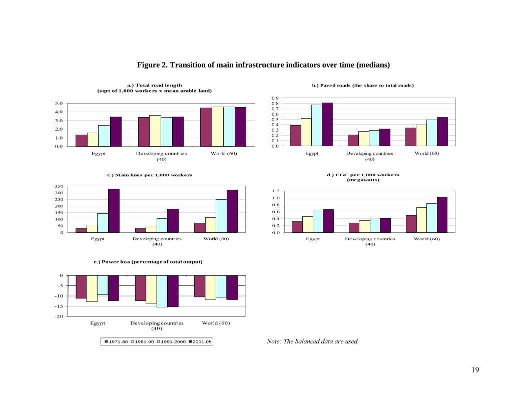
Panels (a) through (e) of Figure 2 display the evolution of the main infrastructure
indicators18: the length of total roads per square root of the country’s 1,000 workers
multiplied by its mean arable land (in km), paved road (the ratio to total road length), the
number of main phone lines per 1,000 workers, and EGC per 1,000 workers (in
megawatts), and power loss (percentage of total output), respectively. In each case, the
group median for each decade is shown.
Transport:
Panel (a) presents road networks as a measure of transport stock and the ratio of
paved roads to total road length as a proxy of transport quality, respectively. We
normalize the measure of transport stock, dividing it by the square root of the country’s
1,000 labor force times its mean arable land. Although Egypt has lagged behind the other
two groups in terms of total road length since the 1970s through the 1990s, the growth in
total road length drastically picked up in the 1990s onwards, while that in the other two
groups has stagnated. As Panel (b) shows, Egypt has far exceeded the typical country in
the two comparator groups regarding the ratio of paved roads to total road length.19
Telecommunications:
Egypt experienced rapid growth in its quantity indicator of telecommunications
over time. As for the number of main lines in Panel (c), the gap between Egypt and
World has significantly narrowed in the latest period.
18 The balanced data is used for all five indicators. 19 We also normalized total road length by 1,000 workers and obtained very similar results to those in Panel (a).
19
Figure 2. Transition of main infrastructure indicators over time (medians)
a.) Total road length(sqrt of 1,000 workers x mean arable land)
0.0
1.0
2.0
3.0
4.0
5.0
Egypt Developing countries(40)
World (60)
b.) Paved roads (the share to total roads)
0.00.10.20.30.40.50.60.70.80.9
Egypt Developing countries(40)
World (60)
c.) Main lines per 1,000 workers
0
50
100
150
200
250
300
350
Egypt Developing countries(40)
World (60)
d.) EGC per 1,000 workers(megawatts)
0.0
0.2
0.4
0.6
0.8
1.0
1.2
Egypt Developing countries(40)
World (60)
-20
-15
-10
-5
0
Egypt Developing countries (40)
World (60)
e.) Power loss (percentage of total output)
1971-80 1981-90 1991-2000 2001-05
Note: The balanced data are used.

20
Electricity:
Panel (d) shows the trends in EGC per 1,000 workers (in megawatts). Egypt exceeds
developing countries in this measure, but has fallen far behind World. The gap between
Egypt and World has even widened in the recent period as growth in EGC has stagnated
in Egypt since the 1990s. The quality indicator of electricity, power loss (in percentage
of total output), displayed in panel (e), improved in the 1990s, but it reversed to the 1980s
level in the most recent period. 20 Although a decline in electricity quality seems to be a
worldwide trend, the electricity sector in Egypt shows some signs of weakening in both
indicators of quality and quantity.
C. Infrastructure Indices by Sector
Some empirical literature that studies the impact of infrastructure on economic
performance uses a single infrastructure sector (i.e. the number of main lines for
telecommunications) as a proxy for infrastructure.21 Others build aggregate indices of
infrastructure quantity and quality that capture the stock of different types of
infrastructure assets and the quality of services in different infrastructure sectors
separately (i.e. quantity and quality indices for telecommunications).22
In this paper, however, instead of focusing on a single sector or building synthetic
indices capturing either quantity or quality aspect of infrastructure assets, we construct
indices by major infrastructure sectors that simultaneously capture both quantity and
quality features of infrastructure. In order to build the sectoral indices, we combine the
information of quantity and quality indicators for the following three sectors,
respectively: transport, telecommunications, and electricity.23
20 The measure of power loss is transformed in a way such that an increase in value indicates an improvement in quality. 21 Easterly (2001) and Loayza, et al (2005). 22 In a series of works by Calderon (2008) and Calderon and Serven (2004, 2008), they constructed synthetic indices of infrastructure quantity and quality, which consist of quantity and quality indicators from the three infrastructure sectors: roads, telecommunications, and power. 23 In order to construct the indices, we used time series data for infrastructure stock and quality indicators in Egypt. When we closely checked the original data, we encountered some issues. That is, some indicators had missing observations, and others fluctuated in an unreasonable way over time. In order to solve these problems, we first interpolated the missing observations for the length of roads and the paved road ratio to

21
The construction of a single infrastructure index per sector is based on the
assumption that both quantity and quality aspects of infrastructure assets are closely
related to and even depend on each other. Consider for example, the electricity sector:
higher power loss (a proxy for quality) may be caused by having too few power plants in
the country and thereby not holding enough electricity generating capacity (a proxy for
quantity) to satisfy the electrical power demand.
For the transport index, we select the length of total roads in km as a measure of
quantity and the ratio of paved roads to total roads as a proxy for quality. As for the
communications index, we use the number of main lines for the physical measure of
communications. As mentioned earlier, the time series coverage of the quality indicator
of telecommunications (telephone faults per 100 main lines) is very limited, and thereby
only the physical measure of telecommunications is used to construct the index. Lastly,
the electricity index consists of electricity generating capacity (EGC) in megawatts and
power loss (percentage of total output) for quantity and quality indicators, respectively.
All stock measures are normalized by 1,000 workers and then transformed in logs. The
exception is total road length, which is normalized by square root of the country’s 1,000
workers multiplied by its surface area.
Table 3. Variance by Sector Using Principal Component Analysis
Sector VarianceTransport 0.7231Telecommunications 1.000Electricity 0.7330Transport & Telecommunications 0.9018
In order to standardize the components for each sector, we use the principal
component analysis (PCA) technique, which allows us to obtain a series of uncorrelated
and normalized linear combinations of the components for each sector. We standardize a total road. Then, we smoothed out some indicators (power loss and paved road ratio), so that the time path in each component became relatively smooth.

22
pair of quantity and quality indicators for each sector (only a quantity indicator for
telecommunications), and then obtain the new index. The principal component for each
sector explains over 70 percent of the variance of the underlying individual indicators, as
shown in Table 3.
Once the three indices are constructed, the transport and telecommunications
indices are combined and transformed into a single new index by using principal
component analysis again. These infrastructure indices: the electricity index, the
transportation index, telecommunications index, and a combined transport and
telecommunications index are used in order to investigate both the effect of infrastructure
on economic growth and the relationship between the performance of infrastructure
assets and infrastructure expenditures in each sector (to be presented in Sections IV and
V).
We now observe the transition of the combined transport and telecommunications
and electricity indices with respect to Egypt’s own history for 1971-2005, given in the
top left panel of Figure 3. Panels (a) through (c) illustrate the time paths of all five
indicators used to construct these indices.
As shown in the top left panel, starting with a negative value, the transport and
telecommunications index was clearly on an upward trend after 1981. After turning to a
positive value in the early 1990s, the index has continued to rise. In fact, the index rose
more than 1.8 point for over three decades. Also starting with a negative value, the
electricity index has been falling during the 1970s and through the mid-1980s (except for
a sharp increase in 1982). After having a positive turn in the mid-1980s, it has been on a
rise along with the transport and telecommunications index for a decade. Reaching its
peak in the late 1990s, the electricity index declined until 2002 but has shown some
recovery in recent years.
As for the components of transport and telecommunications index, Panels (a)
displays a clear upward trend in the length of total roads after the late 1980s, and the ratio
of paved roads to total road length after the early 1980s. For the later, a rise in the
indicator became slow down in the late 1990s. The number of main lines shown in Panel
(b) also illustrates the upward trend, which became more prominent in the early 1980s,
and the indictor continued to rise through recent years. Thus, all three components

23
contribute to a continuous improvement in the transport and telecommunications index
over the last three decades.
Finally, Panel (c) reveals the quite volatile time path of the electricity index which
stems from both components, EGC and power loss. Their trends are clearly more volatile
compared to the other three components used to construct the transport and
telecommunications index.
Having stagnated during the 1970s through the mid-1980s, EGC finally took off
in 1983 and has maintained the level for a decade. After a sharp increase in 1997, it has
continued to fall. As for the other component, power loss rose during the 1970s, declined
through the mid-1980s, and then recovered till 1997. It then fell until recently, where
some signs of improvement are visible.

24
Figure 3. Infrastructure Indices by Sector in Egypt (1971-2005)
-1.2-1.0-0.8-0.6-0.4-0.20.00.20.40.60.81.0
1971 1974 1977 1980 1983 1986 1989 1992 1995 1998 2001 2004
Infrastructure Indices by Sector
Transport & Telecommunications Electricity
(a) Components of Transport Index
-1.8
-1.6-1.4
-1.2
-1.0-0.8
-0.6
-0.4-0.2
0.0
1971 1974 1977 1980 1983 1986 1989 1992 1995 1998 2001 2004
0
0.10.2
0.3
0.40.5
0.6
0.70.8
0.9
Roads, sqrt of 1000 workers x surface area (in logs)
Paved roads (the ratio to total road length)
(b) Components of Telecommunications Index
3.0
3.5
4.0
4.5
5.0
5.5
6.0
1971 1974 1977 1980 1983 1986 1989 1992 1995 1998 2001 2004
Main lines per 1,000 workers (in logs)
0.0
2.0
4.0
6.0
8.0
10.0
12.0
14.0
16.0
18.0
-1.4
-1.2
-1.0
-0.8
-0.6
-0.4
-0.2
0.0
1971 1974 1977 1980 1983 1986 1989 1992 1995 1998 2001 2004
(c) Components of Electricity Index
EGC per 1,000 workers (in logs) Power loss (% of output)

25
IV. Infrastructure and Growth: Regression Analysis
The purpose of this section is to study the effect of infrastructure on the rate of per
capita GDP growth. The goal is to obtain a sensible measure for this effect that can be
used in the quantitative projections for Egypt. To perform our estimations, we use
pooled cross-country and time-series data covering 78 countries over the period 1961-
2005. The data is organized in non-overlapping five-year periods, with each country
having at most 9 observations. The panel is unbalanced, with some countries having
more observations than others. We build on the panel-data growth regression literature
that uses a GMM procedure to address endogeneity and control for unobserved country-
specific factors. This was introduced by Arellano and Bond (1991 and 1998) and applied,
for example, in Levine, Loayza, Beck (2000) and Dollar and Kraay (2004).24 The
econometric methodology is explained in detail in Appendix 3.
A. Data and Regression Specification
Our point of departure is a standard growth regression equation designed for
estimation using (cross-country, time-series) panel data:
' ,,2,11,01,, tiittititititi ICVyyy
(4.1)
Where the subscripts i and t represent country and time period, respectively; y is
the log of output per capita, CV is a set of control variables, and I represents
infrastructure; t and i denote unobserved time- and country-specific effects,
respectively; and is the error term. The dependent variable (yi,t-yi,t-1) is the average rate
of real output growth, that is, the log difference of GDP per capita normalized by the
length of the period. The regression equation is dynamic in the sense that it includes the
level of output per capita (yi,t-1) at the start of the corresponding period in the set of
24 The estimation results presented in the text follow the standard procedure. To check robustness, we applied the standard-error correction proposed by Windmeijer (2005) in exercises not presented here. The qualitative results were, however, the same. In particular, the coefficients related to the infrastructure indices remained statistically significant.

26
explanatory variables. Unless stated otherwise, all data are obtained from the World
Bank’s World Development Indicators.
The set of explanatory variables can be divided into four groups. The first
consists of the initial level of per capita GDP and is included to capture “transitional
convergence,” that is, the tendency of economies to grow slower as they become richer
and converge to their steady state. The second set of variables accounts for the role of
external conditions related to international prices and global economic conditions. To
capture changes in international prices, we use the rate of change of the terms of trade;
and to account for global conditions, we use a period specific dummy variable. The third
group focuses on macroeconomic stability in both aggregate domestic prices and output.
It includes the (log of 1 plus) the CPI inflation rate and a measure of “crisis” volatility
based on negative deviations of trend beyond a certain threshold (see Hnatkovska and
Loayza, 2004, for details).
The fourth group consists of variables that measure structural conditions in areas
such as educational investment, financial depth, trade openness, government burden, and
infrastructure, the variables of particular interest for this study. Educational investment is
measured as (the log of) the gross rate of enrollment in secondary school. Financial
depth is proxied by the ratio of private domestic credit by private financial institutions to
GDP. The outward orientation of the economy is proxied by (the log of) the volume of
trade (exports and imports) to GDP. Government burden is measured as (the log of) the
ratio of general government expenditure to GDP. And infrastructure is measured by the
indices of electric power generation, transportation, and telecommunications, presented in
detail in the previous section.
Except for the variables measuring external conditions, all variables are
potentially jointly endogenous with economic growth (that is, caused by previous and
current innovations in per capita GDP growth, the dependent variable).
B. Estimation Results
We now present and discuss the estimation results. We present different
variations dealing with how the measures of infrastructure are included in the growth
regression. Table 4 presents the estimation results when we include the infrastructures

27
indices one at a time. Table 5 presents the results when we include the indices
simultaneously in the regression.
To establish the validity of our results in the context of the growth literature, let’s
start by analyzing the results corresponding to the standard growth determinants and the
regression specification tests. In brief, the results are consistent with the previous
empirical literature. Initial GDP per capita carries a significantly negative coefficient,
commonly interpreted as evidence of “conditional convergence”; that is, holding constant
(or conditioning for) structural and stabilization conditions, poorer countries tend to grow
faster and, thus, converge towards richer ones. External shocks are also important growth
determinants. Specifically, favorable terms-of-trade shocks affect positively economic
growth. Representing global conditions, the period shifts (not shown in the tables to save
space) indicate that the international trend in economic growth experienced a declining
drift over 1960-2005, resulting in less favorable external conditions in the last three
decades than in the previous ones.
Suggesting a beneficial impact on economic growth, the proxies of educational
investment, depth of financial intermediation, and trade openness have positive and
statistically significant coefficients. Government expenditures, price inflation, and crisis
volatility, on the other hand, carry negative and statistically significant coefficients,
indicating the harmful consequence of government burden and macroeconomic instability.
Finally, regarding the specification tests, the Hansen tests indicate that the null
hypothesis of correct specification cannot be rejected, lending support to our estimation
results. This is the case for all exercises presented below, and we only mention it here in
order to avoid redundancy.
Let’s now focus the discussion on the growth effects of infrastructure. As
mentioned above, in Table 4 we include the infrastructure indices one at a time. They are,
respectively, the electricity index, the transportation index, the telecommunications index,
and a combined transportation and telecommunications index. The latter is relevant for
our purposes because the historical data for Egypt aggregates investment in transportation
and telecommunications. All of them carry positive and significant coefficients. This is
a strong indication that infrastructure in general is an important determinant of economic
growth. It also suggests that each of the aspects of infrastructure considered in the

28
analysis –electricity, transportation, and telecommunications—is relevant for economic
growth. However, this cannot be stated conclusively given that each index can capture
the significance of the rest when they are introduced one at a time in the regression. For
this reason, we turn to Table 5.
In Table 5, the infrastructure indices enter simultaneously in the regression. In
the first column, we introduce the electricity, transportation and telecommunications
indices together. In the second column, we replace the latter two by the combined
transportation and telecommunication index. Interestingly, all infrastructure indices carry
positive and statistically significant coefficients. This indicates that each aspect of
infrastructure considered here is a relevant determinant of economic growth. The size of
the estimated coefficients is also informative. The coefficients presented in Table 5 are
much smaller than those in Table 4, where the indices were introduced one at a time.
This confirms the conjecture mentioned above that each index represents not only its own
specific area but, to some extent, overall infrastructure.
In the next section, we consider in detail the quantitative importance of the
estimated coefficients for the Egyptian case. Here we only consider two brief exercises.
For both, we use the estimated coefficients presented in Table 5, column 1, where the
three basic indices and included simultaneously in the regression. The first exercise is to
consider the growth effect of changing each of the indices by 1 standard deviation of its
world sample distribution. The estimated effects of this improvement are 0.89 percentage
points of per capita GDP growth for electricity, 1.24 for transportation, and 1.26 for
telecommunications. The second exercise is to measure the growth effect of changing
each of the indices from the 25th to the 75th percentile of its world sample distribution.
This is a much larger improvement and, therefore, the estimated growth effects are
correspondingly stronger. They are 1.23 percentage points of per capita GDP growth for
electricity, 2.05 for transportation, and 2.08 for telecommunications.

29
Table 4. Economic Growth and Infrastructure – Individual Effects
Sample: 78 countries, 1961-2005 (5-year period observations)
Estimation Method: System GMM
Infrastructure Variables:
Electricity Index11.539 ***
[6.436]
Transportation Index22.45 ***
[5.631]
Telecommunication Index31.476 ***
[6.687]
Transportation & Telecommunication Index42.81 ***
[7.171]
Control Variables:Initial GDP per capita -1.592 *** -2.072 *** -1.512 *** -2.688 ***
in logs [-5.175] [-5.900] [-7.133] [-7.576]Education 0.949 ** 1.008 *** 0.239 0.367 secondary school enrollment rate, in logs [2.424] [2.973] [0.813] [1.186]Financial Depth 0.403 ** 0.719 *** 1.206 *** 1.075 ***
private credit/GDP, in logs [2.114] [4.226] [7.165] [5.925]Crisis Volatility -1.876 *** -1.734 *** -1.937 *** -1.761 ***
std dev of GDP per capita growth5[-15.070] [-15.400] [-20.300] [-16.120]
Government Burden -0.919 * -0.224 -0.274 0.102 government expenditure/GDP, in logs [-1.957] [-0.429] [-0.611] [0.213]Inflation -0.227 -2.033 *** -3.036 *** -2.841 ***
1+Growth rate of CPI, in logs [-0.362] [-3.189] [-5.071] [-4.561]Trade Openness 4.221 *** 2.062 *** 1.287 ** 1.586 ***
(exports+imports)/GDP, in logs [9.487] [4.358] [2.432] [3.504]Growth rate of Terms of Trade 0.038 *** 0.035 *** 0.046 *** 0.045 ***
log differences of terms of trade index [3.294] [2.942] [4.167] [4.019]Constant 0.733 16.826 *** 21.379 *** 26.997 ***
[0.208] [3.624] [5.036] [5.750]
Observations 522 522 522 522Number of Countries 78 78 78 78Number of Instruments 58 58 58 58Arellano-Bond test for AR(1) in first differences 0.000 0.000 0.000 0.000Arellano-Bond test for AR(2) in first differences 0.064 0.0517 0.134 0.072Hansen test of overidentifying restrictions 0.182 0.357 0.471 0.435
Numbers in brackets are the corresponding t-statistics. * significant at 10%; ** significant at 5%; *** significant at 1%Period fixed effects were included (coefficients not reported).
5 Crisis volatility is the portion of the standard deviation of GDP per capita growth that corresponds to downward deviations below the world-wide 1-std-dev threshold.
1 First principal component of two indicators: power loss (as % of electricity output) & electricity generating capacity (in MW per 1000 workers, in logs).2 First principal component of two indicators: share of paved roads in the overall road network & length of roads (in km, sqrt of per 1000 workers*surface area, in logs).3 First principal component of two indicators: main telephone lines per 1000 workers, in logs & main telephone lines per 1000 workers, in logs.4 First principal component of two indicators: Transportation index & Telecommunication index.
Dependent Variable: GDP per capita Growth
[2] [3] [4][1]

30
Table 5. Economic Growth and Infrastructure –Joint Effects
Sample: 78 countries, 1961-2005 (5-year period observations)
Estimation Method: System GMM
Infrastructure Variables:
Electricity Index10.749 *** 0.975 ***
[5.353] [5.292]
Transportation Index21.093 ***
[3.102]
Telecommunication Index31.097 ***
[4.754]
Transportation & Telecommunication Index42.135 ***
[5.637]
Control VariablesInitial GDP per capita -2.452 *** -2.814 ***
in logs [-8.264] [-8.092]Education 0.604 * 0.668 *
secondary school enrollment rate, in logs [1.749] [1.925]Financial Depth 0.859 *** 0.849 ***
private credit/GDP, in logs [5.486] [5.494]Crisis Volatility -1.679 *** -1.627 ***
std dev of GDP per capita growth5[-18.420] [-13.560]
Government Burden -0.530 -0.413 government expenditure/GDP, in logs [-1.390] [-0.864]Inflation -2.918 *** -2.113 ***
1+Growth rate of CPI, in logs [-6.696] [-3.781]Trade Openness 1.881 *** 2.265 ***
(exports+imports)/GDP, in logs [5.164] [5.657]Growth rate of Terms of Trade 0.060 *** 0.060 ***
log differences of terms of trade index [6.785] [6.424]Constant 26.779 *** 23.764 ***
[7.257] [5.336]
Observations 522 522Number of Countries 78 78Number of Instruments 70 64Arellano-Bond test for AR(1) in first differences 0.000 0.000Arellano-Bond test for AR(2) in first differences 0.170 0.107Hansen test of overidentifying restrictions 0.164 0.340
Numbers in brackets are the corresponding t-statistics.
* significant at 10%; ** significant at 5%; *** significant at 1%Period fixed effects were included (coefficients not reported).
3 First principal component of two indicators: main telephone lines per 1000 workers, in logs & main telephone lines per 1000 workers, in logs.4 First principal component of two indicators: Transportation index & Telecommunication index.5 Crisis volatility is the portion of the standard deviation of GDP per capita growth that corresponds to downward deviations below the world-wide 1-std-dev threshold.
Dependent Variable: GDP per capita Growth
[1] [2]
1 First principal component of two indicators: power loss (as % of electricity output) & electricity generating capacity (in MW per 1000 workers, in logs).2 First principal component of two indicators: share of paved roads in the overall road network & length of roads (in km, sqrt of per 1000 workers*surface area, in logs).

31
V. Infrastructure Investment and Growth in Egypt
A. Trends in Infrastructure Investment
We now turn to reviewing the long-term trends in infrastructure investment in
Egypt. The investment data are disaggregated by sector of origin: public and private, and
by destination of industry. Infrastructure investment includes both capital expenditures
(the construction of new infrastructure) and current expenditures (operations and
maintenance spending).
There are two kinds of time series data available for Egypt’s infrastructure
investment. The first data range from 1960 through 2007 with the disaggregation of two
infrastructure sectors: transportation (including Suez Canal) and communications, and
electricity. The second data cover the more recent period: 2003-2007, with a higher
degree of disaggregation, that is, five infrastructure sectors: transportation,
communications, electricity, water, and Suez Canal.
Figure 4 offers a comprehensive view of infrastructure investment in Egypt
relative to GDP from 1960 through 2007. Panel (a) of Figure 4 illustrates the time path
of total infrastructure investment that consists of investment in two infrastructure sectors:
transportation and communications and electricity, with a disaggregation of public and
private investment. Total investment rose until the late 1980s, and then it declined until
the mid 2000s, when it stabilized. Total investment in recent years has returned to its
level in the early 1960s at roughly 5 percentage of GDP. It is clear that public investment
has been a dominant force for more than four decades in Egypt. In contrast, after having
stagnated for more than two decades since the 1960s, private investment finally took off
in the mid-1980s. The magnitude of private investment has been growing and is roughly
two-thirds of the amount of public investment in recent years. Though considerable,
rising private investment in the last two decades has not fully offset the decline in public
investment.
From Panels (b) and (c) of Figure 4, there is an apparent downward trend in total
investment which originated from a decline in public investment in both the
transportation/communications and electricity sectors. Public investment in the former
has been declining since the early 1980s, while that in the later since the late 1980s.

32
Figure 4. Infrastructure Investment in Egypt (1960-2007)
(Percentage of GDP)
(c) Electricity
0.0
1.0
2.0
3.0
4.0
5.0
6.0
1960 1965 1970 1975 1980 1985 1990 1995 2000 2005
Public Private
(b) Transportation (incl. SC) & Communications
0.0
2.0
4.0
6.0
8.0
10.0
1960 1965 1970 1975 1980 1985 1990 1995 2000 2005
(a) Total Investment
0.0
2.0
4.0
6.0
8.0
10.0
12.0
14.0
1960 1965 1970 1975 1980 1985 1990 1995 2000 2005

33
Conversely, private investment in transportation and communications has maintained its
level after its sharp increase in the mid-1980s and has been on the rise again in recent
years. Private participation in the electricity sector is still quite limited.
Figure 5 depicts the time path of more recent investment for 2003-2007 by
destination of five infrastructure sectors and by sector of origin. In particular, investment
data in the three core infrastructure sectors (transportation, communications, and
electricity) are presented separately, allowing a more precise assessment of their recent
trends.25
As shown in Panels (a) through (e) of Figure 5, the shares of investments in both
water and Suez Canal are quite small compared to three core sectors. Investment in the
water sector increased drastically in 2007, while that in Suez Canal has fallen since 2004.
In additions, the figure reveals that public sector continues to play a major role in
investment in electricity, water, and Suez Canal.26
Repeating the findings in Figure 4, public investment in transportation,
communications, and electricity has been falling, while a rise in private investment has
become more obvious in transportation and communications in recent years. In particular,
the private sector has become a dominant player in investment in the communications
sector since 2005.
B. Cross-Country Comparison of Infrastructure Investment
In this section, we compare the level of infrastructure investment in Egypt to that
of other developing countries. Panels (a)–(c) of Figure 6 plot infrastructure investment
(total, public, and private) as ratio to GDP for 2000-05 against GDP per capita in 2000
across countries.27 Total and public infrastructure investment fall as the income level of
the country increases, while the opposite happens for private investment.
25 In Appendix 4, we present disaggregated investment data for transportation (including investment in Suez Canal) and communications as ratio to GDP for 1983-2007 (see Figure 4-A). These data has been made available only recently. 26 There is no private investment for water and Suez Canal. As for electricity, no private investment has been carried out after 2004. 27 Infrastructure investment data are obtained from Calderon, Odawara, and Serven (2008). Total investment consists of investment in three major infrastructure sectors: transport, telecommunications, and electricity.

34
Figure 5. Infrastructure Investment in Egypt (2003-2007) (Percentage of GDP)
(a)Transportation
0.0
0.5
1.0
1.5
2.0
2.5
3.0
2003 2004 2005 2006 2007
(b) Communications
0.0
0.2
0.4
0.6
0.8
1.0
1.2
1.4
2003 2004 2005 2006 2007
(c) Electricity
0.0
0.5
1.0
1.5
2.0
2003 2004 2005 2006 2007
Public Private

35
Figure 5 (continued). Infrastructure Investment in Egypt (2003-2007) (Percentage of GDP)
(d) Water
0.0
0.1
0.2
0.3
0.4
0.5
0.6
2003 2004 2005 2006 2007
(e) Suez Canal
0.00
0.02
0.04
0.06
0.08
0.10
2003 2004 2005 2006 2007
Public Private

36
This may indicate that poorer countries, especially through their public sectors,
tend to make larger infrastructure investments until they build a certain level of
infrastructure assets (a number of electricity plants and a road network). As they become
richer, they tend to spend less in new infrastructure, focusing on maintaining existing
assets. Panels (a) shows that Egypt is located on the predicted regression line for total
investment. In contrast, for public and private investment Egypt shows interesting
discrepancies with respect to the international norm (Panels (b) and (c)). While public
investment in infrastructure in Egypt is much larger than what would be expected
according to the country’s income level, its private investment is considerable smaller
than the standard set by other developing countries.
Finally, we turn to reviewing the trends of infrastructure investment across
countries. Figures 7.1 and 7.2 provide an overview of the level of infrastructure
investment in six countries, divided into two groups: India (IND), Pakistan (PAK), and
Indonesia (IDN) in Figure 7.1, and Egypt (EGY), Turkey (TRK), and South Africa (SA)
in Figure 7.2. Panels (a) through (c) of Figures 7.1 and 7.2 offer the trends of total,
public, and private investment as a share of GDP for over the last two decades,
respectively.
The top panels of Figures 7.1 and 7.2 illustrate that total investment has been
slightly falling over time. This tendency is more obvious in the mid 1990s or the early
2000s, when even countries which investment had remained roughly constant over time
(i.e. India, Pakistan, and Turkey) experienced a downward trend. The middle panel
shows that the path of public investment has been declining in all six countries. In
contrast, private investment, shown in the bottom panel, presents a clear upward trend
(except for Indonesia). Private investment in infrastructure has increased so much than it
has equaled and, in some cases, even surpassed public investment.
Thus, public and private investments display contrasting patterns, which indicates
that those countries have experienced a composition shift between public and private
investment. The share of private investment to total investment has been rising, while
that of public investment has been falling. However, rising private investment has not
fully offset the fall in public investment in most cases.

37
Figure 6. Infrastructure Investment (average of 2000-05, % of GDP)
MNGKHM
PAK
VNM
IND
BOL
IDN
EGY
PHL
JOR
PER
COL
THA
TRK
BRASA
CHL
MEXARG
EGY
24
68
10To
tal Inf
rastru
ctur
e In
vestm
ent (
% o
f GDP)
7 8 9 10Log per capita GDP at year 2000
(a) Total Investment
MNGKHM
PAK
GEO
VNM
IND
BOL
ARMIDN
EGY
MAR
ALB
PHL
UKR
JOR
PER
BLR
DZA
COL
THA
TRK
BRALVA
LTU
SACHL
MEX
SVK
ARG
HUN
SVN
EGY
02
46
8Pub
lic In
frastru
ctur
e In
vestm
ent (
% o
f GDP)
7 8 9 10Log per capita GDP at year 2000
(b) Public Investment
MNGKHM
PAKVNM
IND
BOL
IDN
EGY
PHLJOR
PER
COL
THA
TRK
BRA SA
CHL
MEX
ARGEGY
01
23
4Pr
ivat
e In
frastru
ctur
e In
vestm
ent (
% o
f GDP)
7 8 9 10Log per capita GDP at year 2000
(c) Private Investment
Data source: Calderón, Odawara, and Servén (2008).

38
Figure 7-1. Infrastructure Investment across Countries (percentage of GDP)
(a) Total Investment
012345678
1981 1984 1987 1990 1993 1996 1999 2002 2005
(b) Public Investment
0.00.51.01.52.02.53.03.54.04.55.0
1981 1984 1987 1990 1993 1996 1999 2002 2005
(c) Private Investment
0.0
0.5
1.0
1.5
2.0
2.5
3.0
1981 1984 1987 1990 1993 1996 1999 2002 2005
IND PAK IDN
Data source: Calderón, Odawara, and Servén (2008).

39
Figure 7-2. Infrastructure Investment across Countries
(percentage of GDP)
(a) Total Investment
0
2
4
6
8
10
12
14
1980 1985 1990 1995 2000 2005
(b) Public Investment
0
2
4
6
8
10
12
1980 1985 1990 1995 2000 2005
(c) Private Investment
0
1
2
3
4
5
6
1980 1985 1990 1995 2000 2005
EGY TRK SA
Data source Calderón, Odawara, and Servén (2008).
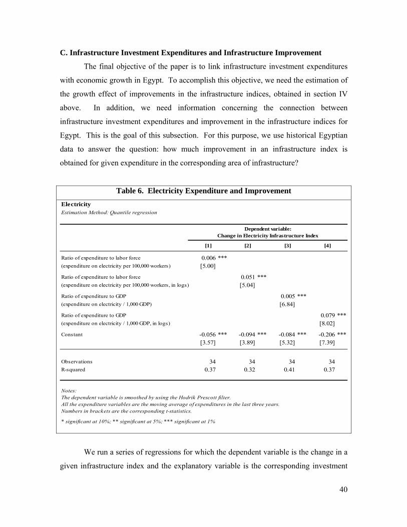
40
C. Infrastructure Investment Expenditures and Infrastructure Improvement
The final objective of the paper is to link infrastructure investment expenditures
with economic growth in Egypt. To accomplish this objective, we need the estimation of
the growth effect of improvements in the infrastructure indices, obtained in section IV
above. In addition, we need information concerning the connection between
infrastructure investment expenditures and improvement in the infrastructure indices for
Egypt. This is the goal of this subsection. For this purpose, we use historical Egyptian
data to answer the question: how much improvement in an infrastructure index is
obtained for given expenditure in the corresponding area of infrastructure?
Table 6. Electricity Expenditure and Improvement
ElectricityEstimation Method: Quantile regression
Ratio of expenditure to labor force 0.006 ***(expenditure on electricity per 100,000 workers) [5.00]
Ratio of expenditure to labor force 0.051 ***(expenditure on electricity per 100,000 workers, in logs) [5.04]
Ratio of expenditure to GDP 0.005 ***(expenditure on electricity / 1,000 GDP) [6.84]
Ratio of expenditure to GDP 0.079 ***(expenditure on electricity / 1,000 GDP, in logs) [8.02]
Constant -0.056 *** -0.094 *** -0.084 *** -0.206 ***[3.57] [3.89] [5.32] [7.39]
Observations 34 34 34 34R-squared 0.37 0.32 0.41 0.37
Notes:The dependent variable is smoothed by using the Hodrik Prescott filter.All the expenditure variables are the moving average of expenditures in the last three years.Numbers in brackets are the corresponding t-statistics.
* significant at 10%; ** significant at 5%; *** significant at 1%
Dependent variable: Change in Electricity Infrastructure Index
[4][1] [2] [3]
We run a series of regressions for which the dependent variable is the change in a
given infrastructure index and the explanatory variable is the corresponding investment

41
expenditure in average for the previous three years. Investment expenditure is
normalized in different ways. We consider, in turn, the ratio of expenditure to the labor
force and the ratio of expenditures to GDP; and in addition, we consider the logarithm of
each of these two ratios. As mentioned above, publicly available Egyptian historical data
has not (until recently) disaggregated between the transportation and telecommunication
sectors;28 therefore, we use the infrastructure index that combines those two sectors. For
electricity, on the other hand, there is sector specific expenditure data; and therefore, we
use its own infrastructure index. The results are presented in Table 6 for electricity and
Table 7 for transport and telecommunications.29
Table 7. Transportation and Telecommunication Expenditures and Improvement
Transportation and TelecommunicationEstimation Method: Quantile regression
Ratio of expenditure to labor force 0.002 ***(expenditure on transportation & telecommunication per 100,000 workers) [14.22]
Ratio of expenditure to labor force 0.038 ***(expenditure on transportation & telecommunication per 100,000 workers, in logs) [9.46]
Ratio of expenditure to GDP 0.002 ***(expenditure on transportation & telecommunication / 1,000 GDP) [5.08]
Ratio of expenditure to GDP 0.061 ***(expenditure on transportation & telecommunication / 1,000 GDP, in logs) [3.96]
Constant -0.016 *** -0.076 *** -0.036 ** -0.18 ***[3.84] [6.16] [2.08] [3.16]
Observations 45 45 45 45R-squared 0.47 0.44 0.19 0.22
Notes:All the expenditure variables are the moving average of expenditures in the last three years.Numbers in brackets are the corresponding t-statistics.
* significant at 10%; ** significant at 5%; *** significant at 1%
Dependent variable: Change in Transportation & Telecommunication
Infrastructure Index
[4][1] [2] [3]
28 As stated in footnote 24, disaggregated investment data for transportation and telecommunication has recently become available for the period 1983-2007. It is not used here, however, because of its limited time coverage and because it has not undergone the necessary quality controls. 29 These regressions are estimated using the Quantile (Median) estimator, rather than the simpler and more common Ordinary Least Squares procedure. Although the results from both methods are similar to each other, in this case we prefer the Quantile estimator given its lower sensitivity to outlier observations.

42
The results are qualitatively similar for both electricity and
transportation/telecommunications. The coefficients on the four measures of investment
expenditure are positive and statistically significant, implying that there is a relevant
connection between investments and improvement in infrastructure. However, the small
size of the coefficients, as well as the low R2s, reveals that any economically important
improvement in the infrastructure indices would take a relatively long time if investment
expenditures are maintained at moderate levels. A rapid improvement in the indices
would occur only under quite sizable investment. Since most public expenditure
planning is done relative to GDP, in what follows we only use the estimated coefficient in
Column 3 of each table.
In addition, we conduct a more complex regression analysis of infrastructure
improvement by linking it not only to investment expenditures but also to the current
stock of infrastructure. This extension may be necessary to take into account the
infrastructure “product cycle,” that is, the different investment needs at different stages of
infrastructure development. In most infrastructure cases, larger investment is needed
when infrastructure is incipient, as when it depends on expensive plants to initiate
production. This is known in the economics literature as “non-convex investment,”
characterized by large fixed costs and low marginal costs. In other cases, initial
infrastructure improvements may be obtained relatively easily; but as development occurs,
further progress is increasingly costly.
We conduct this extended empirical analysis by estimating a regression of the
change in infrastructure index on past investment expenditure, the current infrastructure
index, and the interaction between the two. The results are presented in Appendix 5. For
electricity, the three explanatory variables are statistically significant, carrying the
following pattern of signs. The respective coefficient on investment expenditure is
positive, on current infrastructure index is negative, and on the interaction is positive.
The positive coefficients on both investment expenditure and its interaction with the
current infrastructure level indicate that electricity-related infrastructure behaves as “non-
convex” investment, that is, electricity improvements are more costly in the early stages
of this type of infrastructure, when large plants and generators have to be constructed. As
electricity infrastructure develops, there is a larger expansion in infrastructure for given

43
amount of expenditures. For transport and telecommunications, the pattern of signs is the
same, although only the investment expenditure and, in one case, its interaction with
current infrastructure level are statistically significant. Given that both of these variables
carry positive coefficients, the results indicate that the transport and telecommunications
sector is also characterized by necessary large outlays at incipient levels of progress, with
lower costs afterwards.30
Notwithstanding their insightfulness, the results on the complex specification of
the infrastructure regression are more tentative than those of the simple specification
presented above because of data constraints and robustness concerns. Since the simple
specification implies constant costs to infrastructure improvement (rather than declining
ones, as in the complex specification), using the simple specification results entails a
more conservative approach to growth projections. We use the simple specification
results in order to produce more conservative projections and because we are more
confident in the quality of its estimates.
D. Growth Projections
We are now ready to produce the main projections of the paper; that is, the
projections on growth improvement given an increase in public infrastructure
expenditures. For this purpose, we need three pieces of information. The first relates to
the determinants of economic growth. From this analysis, the most important element to
consider is the effect of the infrastructure indices on economic growth. We also need to
consider that a rise in infrastructure entails an increase in investment expenditures, which
may involve a corresponding increase in the government burden (through distortionary
taxation, public debt overhang, or bureaucratic red tape). Lastly, we must take into
account that improving growth becomes more difficult as per capita GDP gets larger (the
convergence effect). These effects are measured through the estimated coefficients on,
respectively, the two infrastructure indices, the proxy of government burden, and the
initial level of per capita GDP, which we take from Table 5, Col. 2.
30 The negative coefficient on current infrastructure stock (attenuated by the positive coefficient on the interaction) can be interpreted as an indication of capital depreciation.

44
The second piece of information is the effect of infrastructure expenditure on
improvements in the infrastructure indices in Egypt. These parameters are obtained from
the analysis on electricity and transportation/telecommunication improvements;
specifically, we use the estimated coefficients reported in Tables 6 and 7, Col. 3. The
third piece of information is the projected new level of infrastructure expenditure. In
recent years, total infrastructure expenditures in Egypt are about 5% of GDP, allocated
around 1.3% to electricity and 3.7% to transportation and telecommunication. For
projected expenditures, we consider three scenarios. In the first, we allow total
infrastructure expenditures to increase from 5% to 6% of GDP permanently. In the
second one, the increase is substantially larger, from 5% to 8% of GDP permanently. In
the third scenario, we consider a large initial increase that gradually diminishes over time.
Specifically, infrastructure expenditures rise from 5% to 7% of GDP for the first twenty
years, then decline to 6.5% of GDP for the following 20 years, and thereafter converge to
6% of GDP forever. In all cases, the increase is allocated proportionally to expenditures
for electricity and transportation/telecommunication.
Figure 8: Projected Growth Improvement from Higher Infrastructure Investment
0.00
0.50
1.00
1.50
2.00
2.50
3.00
3.50
4.00
0-5 5-10 10-15 15-20 20-25 25-30 30-35 35-40 40-45 45-50
%
Five-year periods
Growth Improvementwith respect to current infrastructure spending of 5%GDP
Scenario 1: 6% GDP Scenario 2: 8% GDP Scenario 3: 7/6.5/6% GDP

45
Figure 8 presents the growth projections under the three scenarios for the next 50
years. They represent the change in growth with respect to the path corresponding to the
current infrastructure investment of 5% of GDP. The growth improvement is not
constant over time because, first, as the infrastructure stock builds up, it renders higher
growth; and, second, as per capita GDP rises, it becomes more difficult to grow further.
In addition, the government burden of increased expenditures reduces the growth
improvement. These three forces play against each other dynamically to render the
projected growth path. The effect of higher infrastructure investment dominates over
time, and that’s why the growth improvement path rises gradually.
In the first years of larger infrastructure investment, the growth returns are rather
small. However, towards the end of the first decade, the per capita GDP growth
improvement is already considerable, reaching almost 0.5 pp, 1.5 pp, and 1 pp for three
scenarios, respectively. By the third decade, the growth improvement continues to rise,
amounting to 1 pp, 3 pp, and 1.75 pp, correspondingly for the three scenarios. Note that,
by the design of the third scenario, its growth improvement tends to flatten by the fifth
decade. As time goes on, the infrastructure stock continues to increase, promoting larger
growth; however, due to decreasing returns (manifested through conditional convergence
in the growth regression), these growth improvements are increasingly harder to obtain.
The combination of these two forces makes the growth improvement converge to a
steady value. Specifically, in the long run, the growth gains from the three scenarios are,
respectively, 1.6 pp, 4.7 pp, and 1.6 pp. The first and third scenarios render the same
long run increase because in both cases infrastructure expenditure eventually stays at 6%
of GDP.
The projections just presented assume, realistically, that the increase in
infrastructure investment may involve a heavier government burden (through higher
government expenditures). However, if the rise in infrastructure investment occurs in the
context of public expenditure reform, entailing a redistribution of funds from less to more
efficient uses and a co-participation of the private sector in the investment process, then
the growth improvement could become substantial even in the first years of the program.
Figure 9 compares the results for the first two scenarios (i.e., a permanent increase of
infrastructure investment to 6% and 8% of GDP, respectively) between low and high

46
government burden. High government burden corresponds to the projections analyzed
above (and presented in Figure 8). Low government burden corresponds to the case
when the increase in infrastructure investment does not imply an increase in government
expenditures (setting the corresponding coefficient to zero). The results are remarkable.
Having a low government burden is crucial to increase the growth improvement from
higher infrastructure investment particularly in the early stages of the program. Even
when the increase in infrastructure investment is modest (from 5% to 6% of GDP), the
per capita GDP growth improvement can reach 1 pp by the end of the first decade
provided the government burden is low (this rise is twice as high as under high
government burden). If government burden is a big concern, it may be better to increase
infrastructure investment by a modest amount, particularly in the first years. An
implication from this analysis is that the merits of increasing infrastructure investment
have to be weighed against the costs of an expansion in government size. One way to
deal with this challenge is to increase the quality of infrastructure investment by giving
the private sector a more active role in the provision of infrastructure.
Figure 9: Projected Growth Improvement under Different Fiscal Burden
0.00
0.50
1.00
1.50
2.00
2.50
3.00
3.50
4.00
4.50
0-5 5-10 10-15 15-20 20-25 25-30 30-35 35-40 40-45 45-50
%
Five-year periods
Growth Improvementcomparing low and high government burden to increase infrastructure expenditure
6% GDP, Low Burden 6% GDP, High Burden 8% GDP, Low Burden 8% GDP, High Burden

47
The simulations can be used to inform three critical values used in public policy
analysis. The first is the measure of the fiscal multiplier. This is the impact on per capita
GDP of a given increase in public expenditures. The simulations show that the fiscal
multiplier that applies to infrastructure expenditures gradually rises over time. A
permanent increase in public infrastructure expenditures of 1 percentage point of GDP
leads to a positive but small change in per capita GDP in the first few years of
implementation. The low short-term impact is explained by the fact that infrastructure
takes time to build, while the negative impact of government burden is rather immediate.
As the stock of infrastructure grows, so does the positive effect on per capita GDP. Thus,
the fiscal multiplier reaches 1 percentage point of per capita GDP about three decades
after implementation, gradually converging to a long-run fiscal multiplier of 1.6
percentage points.
The second is the analysis of financial fiscal sustainability. Specifically the issue
is whether the improvement in infrastructure can render a sufficient increase in
government revenues to fully finance infrastructure investment. In layman's terms: does
public infrastructure pay for itself? According to our simulations, if the proceeds derived
from the new infrastructure projects are limited to general government revenues, public
infrastructure investment will not pay for itself. In Egypt, government revenues amount
to 25-30% of GDP. Applying this range of rates, the rise in government revenues given
by the increase in GDP will only cover a fraction of the increase in infrastructure
expenditure. This fraction would be rising given the increasing impact of infrastructure
investment on GDP growth. Thus, assuming a government revenue rate of 30% of GDP,
the fraction of self-finance infrastructure investment would be about 35% during the first
five years, 50% by the end of the second decade, and 75% in the long run.
(Correspondingly, the revenue rates needed for infrastructure investment to break even
would be 85%, 60%, and 40% for the respective time horizons.)
The third, and most important, is the analysis from a social perspective. This
considers the value of the increase in per capita GDP (or income) for society as a whole.
The calculation should take into account the time value of money and, therefore, discount
the future stream of income with an appropriate rate. Assuming a discount rate of 5%
over the per capita GDP growth rate, an increase in infrastructure expenditure of 1

48
percentage point of GDP leads to a net present value gain of 6 percentage points of per
capita GDP for the first 25 years of implementation and 10.5 percentage points of per
capita GDP for the first 50 years.31 This is a sizable yet reasonable improvement, and it
can be further increased if the program's financing and implementation are less
burdensome to the economy. Finally, we must note that this improvement is only a
fraction of the total effect of infrastructure on social welfare. A complete evaluation
would also take into account the direct benefit of infrastructure on the health, comfort,
and happiness of its recipients.
VI. Summary and Conclusion
In the last half century, Egypt has experienced remarkable progress in the
provision of infrastructure, which is the result of decades of purposeful and costly
investment. In the past 15 years, however, a worrisome trend has emerged: Infrastructure
investment has suffered a substantial decline. To be sure, some of this decrease is to be
expected as infrastructure projects mature and demand less costly outlays. Nevertheless,
the investment decline should be of concern for two reasons. The first is that the rate of
progress in the measures of infrastructure, particularly road networks and power
generation, has slowed down. A developing country like Egypt cannot afford such
stagnation. The second reason is that, although acceptable at Egypt’s current income
level, infrastructure in the country has much room to improve to be consistent with its
goals of future economic growth.
The study first reviews the current state of several infrastructure indicators in
Egypt compared with the rest of the world. For this purpose, a dataset for 150 countries
was collected containing different indicators of quantity and quality of services for four
major sectors of infrastructure: transport, telecommunications, electricity, and water and
sanitation. The overall results suggest that Egypt has attained a level of infrastructure
31 The first-order condition for consumer welfare maximization implies, r = ρ + σ g, where r is the real interest rate, ρ is the subjective rate of time preference, σ is the inverse of the coefficient of intertemporal substitution, and g represents the per capita GDP growth rate. It is customarily assumed that the coefficient of intertemporal substitution is equal to 1 and the subjective rate of time preference is 0.05. This would entail a real interest rate equal to 0.05 over the growth rate, which is our working assumption here. Thus, if the per capita GDP growth rate were around 5%, the real interest used as discount rate in the NPV calculations would be 10%.

49
performance consistent with what is expected given its level of economic development.
In particular, Egypt performs as well as or better than other countries of similar per
capita GDP regarding the following infrastructure indicators. For transportation: road
network length, paved roads, quality of railroads, and quality of air transport. For
telecommunication: main telephone lines, telephone faults, and waiting list of mainline
installation. For power generation and water: access to electricity, quality of electricity
supply, access to improved water source, and access to sanitation facilities.
Then, the study examines the trends in infrastructure spending in Egypt from
1960 to 2007, disaggregated by sector of origin (public and private) and by two main
sectors, transportation (including Suez Canal) and communications, and electricity.
Relative to GDP, total infrastructure expenditure in Egypt fell after reaching its peak in
the late 1980s, mainly due to a decline in public spending. Private investment took off
in the mid-1980s, and its magnitude has been growing since then. In recent years, the
rise in private investment is clear in transportation and telecommunications, with the
private sector becoming a principal player in telecommunications since 2005. Rising
private investment in the last two decades, however, has not entirely offset the decline in
public spending.
In comparison with other developing countries, the share of public in total
infrastructure spending in Egypt is larger than what would be expected according to the
country’s income level. In contrast, by the same standard its private infrastructure
spending is considerably smaller. The trends of infrastructure expenditure across
countries also reveal declining public spending and a clear upward trend in private
investment. Thus, not only Egypt but countries such as India, Indonesia, Pakistan,
South Africa, and Turkey have experienced a composition shift from public to private
infrastructure spending. In some cases, such as India and Turkey, private investment
has increased sufficiently to offset the decline in public spending in infrastructure.
A large body of literature has found that improving infrastructure has a
statistically significant and economically substantial positive effect on economic growth.
Using data for 78 countries for the period 1960-2005, this study confirms the result on the
beneficial growth impact of infrastructure in telecommunication, transport, and power
generation. This impact is found to be larger if infrastructure development does not

50
involve an increase in government burden on the economy. Moreover, using Egypt-
specific data, the study finds a positive and significant link between infrastructure
expenditures and infrastructure development. Based on these results, this study
concludes that improving infrastructure in Egypt will have a beneficial effect on
economic growth and that, in turn, improving infrastructure will require a combination of
larger infrastructure expenditures and more efficient investment.
The analysis provided in this study suggests that a permanent increase in
infrastructure expenditures has a gradually rising effect on per capita GDP growth. As
the infrastructure stock builds up, it renders higher growth; on the other hand, as per
capita GDP rises, it becomes more difficult to grow (due to diminishing capital returns).
In addition, the government burden of increased expenditures may reduce any growth
improvement. These three forces play against each other dynamically to render the
projected growth path of a permanent rise in infrastructure expenditure. The effect of
higher infrastructure investment dominates over time, and, thus, economic growth rises
gradually to converge to a positive value.
The quantitative estimates obtained in this study allow some tentative growth
projections. If infrastructure expenditure in Egypt rose permanently from its current level
of 5% of GDP to 6%, the growth returns would be rather small in the first years but
would gradually rise. Towards the end of the first decade, the gain in per capita GDP
growth would reach almost 0.5 percentage points, by the third decade it would amount to
1 percentage point, and eventually it would converge to 1.6 percentage points. If the
increase in infrastructure expenditures were more pronounced, from 5% to 8%, the rise in
per capita GDP growth would amount to 1.5, 3, 4.7 percentage points in the
corresponding time horizons.
These quantitative estimates can be used to elucidate questions of fiscal
sustainability and social welfare. First, on financial fiscal sustainability, the issue is
whether the improvement in infrastructure can render a sufficient increase in government
revenues to fully finance infrastructure investment. According to the simulations
presented in the study, if the proceeds derived from the new infrastructure projects were
limited to general government revenues, public infrastructure investment would not pay
for itself. Considering the rates of government revenues prevailing in Egypt (25-30% of

51
GDP), the rise in government revenues given by the increase in GDP would only cover a
fraction of the increase in infrastructure expenditure. This fraction would be rising given
the increasing impact of infrastructure investment on GDP growth. Thus, the fraction of
self-finance infrastructure expenditure would be about 35% during the first five years,
50% by the end of the second decade, and 75% in the long run. Second, on social
welfare, the estimates can be used to quantify the gains from an expansion in
infrastructure in terms of per capita GDP. The calculation should take into account the
time value of money and, therefore, discount the future stream of income with an
appropriate rate. Assuming a discount rate of 5% over the per capita GDP growth rate,
an increase in infrastructure expenditure of 1 percentage point of GDP would lead to a
net present value gain of 6 percentage points of per capita GDP for the first 25 years of
implementation and 10.5 percentage points of per capita GDP for the first 50 years.
These projections assume, realistically, that the increase in infrastructure
expenditure may involve a heavier government burden (through higher government
expenditures). However, if the rise in infrastructure expenditure occurs in the context of
public expenditure reform, entailing a redistribution of funds from less to more efficient
uses and a co-participation of the private sector in the investment process, then the
growth improvement could become substantial even in the first years of the program. If
infrastructure expenditure rose permanently from 5% to 6% of GDP without entailing
more government burden, the per capita GDP growth improvement could reach 1
percentage point by the end of the first decade. If government burden is a big concern, it
may be better to increase infrastructure investment by a modest amount, particularly in
the first years.
One implication from this analysis is that the merits of increasing infrastructure
investment have to be weighed against the costs of an expansion in government size. A
second implication is that renewed infrastructure investment should be considered in the
larger context of public sector reform. Rationalizing public expenditures can release
resources to be used in the generation of infrastructure. Moreover, an improvement in the
quality of infrastructure investments can result in faster progress at lower costs. In this
regard, Egypt would do well in considering the experience of other countries where

52
stronger participation of the private sector in the provision of infrastructure has led to
significant productivity gains.
Finally, a limitation of this study should be acknowledged. It has focused on the
economic growth impact and corresponding income improvement obtained from higher
infrastructure investment. This is, however, only one of the positive effects of
infrastructure on social welfare. A complete evaluation would also take into account the
direct benefit of infrastructure on people’s health, accessibility, comfort, and, ultimately,
happiness.

53
References
Agenor, Pierre-Richard, Nabli, Mustapha K., and Tarik M. Yousef (2005). “Public Infrastructure and Private Investment in the Middle East and North Africa.” World Bank Policy Research Working Paper 3661. The World Bank. Alonso-Borrego, C. and M. Arellano (1999). “Symmetrically Normalized Instrumental-Variable Estimation Using Panel Data.” Journal of Business and Economic Statistics 17(1): 36-49. Arellano, M., and S. Bond (1991). “Some Tests of Specification for Panel Data: Montecarlo Evidence and an Application to Employment Equations.” Review of Economic Studies 58(2): 277-97. _____ (1998). “Dynamic Panel Data Estimation Using DPD98 for Gauss: A Guide for Users.” Mimeo. CEMFI. ftp://ftp.cemfi.es/pdf/papers/ma/dpd98.pdf Arellano, M., and O. Bover (1995). “Another Look at the Instrumental-Variable Estimation of Error-Components Models.” Journal of Econometrics 68(1): 29-52. Aschauer, David A. (1989). “Is Government Spending Productive?” Journal of Monetary Economics 23:177-200. Arrow, Kenneth, J. and Mordekai Kurz (1970). “Public Investment, The Rate of Return and Optimal Fiscal Policy.” Johns Hopkins. Barro, Robert J. (1990). “Government Spending in a Simple Model of Endogenous Growth.” The Journal of Political Economy 98 (5): 103-125. ______, (1991). “Endogenous Growth in a Cross Section of Countries.” Quarterly Journal of Economics 106: 404-444. Barro, Robert J. and Xavier Sala-I-Martin (1992). “Public Finance in Models of Economic Growth.” Review of Economic Studies 59: 645-661. Blundell, R. and S. Bond (1998). “Initial Conditions and Moment Restrictions in Dynamic Panel Data Models.” Journal of Econometrics 87(1): 115-143. Calderon, Cesar (2008) “Infrastructure and Growth in Africa,” Unpublished working paper, The World Bank. Calderon, Cesar and Alberto Chong (2004). “Volume and Quality of Infrastructure and the Distribution of Income: An Empirical Investigation.” Review of Income and Wealth 50: 87-105.

54
Calderon, Cesar and Luis Serven (2004). “The Effects of Infrastructure Development on Growth and Income.” World Bank Policy Research Working Paper No. 3400. The World Bank. _____ (2004). “The Trends in Infrastructure in Latin America.” World Bank Policy Research Working Paper 3401. The World Bank. _____ (2008). “Infrastructure and Economic Development in Sub-Saharan Africa.” World Bank Policy Research Working Paper No. 4712. The World Bank. Calderon, Cesar, Odawara, Rei, and Luis Serven (2008). "Infrastructure Investment in Developing Countries: A Quarter-Century Retrospective." Mimeo. The World Bank. Canning, David (1999). “The Contribution of Infrastructure to Aggregate Output.” World Bank Policy Research Working Paper 2246. The World Bank. Canning, David and Marianne Fay (1993). “The Effect of Transportation Networks on Economic Growth.” Columbia University Department of Economics Discussion Paper Series. Columbia University. Demitoriades, Panicos O. and Theofanis P. Mamuneas (2000). “Intertemporal Output and Employment Effects of Public Infrastructure Capital: Evidence from 12 OECD Economies.” Economic Journal, Royal Economic Society 110(465): 687-712. Devarajan, Shantayanan, Swaroop, Vinaya, and Heng-Fu Zou (1996). “The Composition of Public Expenditure and Economic Growth.” Journal of Monetary Economics 37: 313-344. Dhumale, Rahul (2000). “Public Investment in the Middle East and North Africa: Towards Fiscal Efficiency,” Development Policy Review Vol.18, pp.307-324. Dobronogov, Anton, and Farrukh Iqbal (2005). “Economic Growth in Egypt: Constraints and Determinants.” MENA Working Paper Series No. 42. The World Bank. Dollar, D. and A. Kraay (2004). “Trade, Growth, and Poverty.” Economic Journal 114(493): F22-49. Easterly, William (2001). “The Lost Decades: Explaining Developing Countries’ Stagnation in spite of Reform 1980-98.” Journal of Economic Growth 6 (2): 135-157. Easterly, William and Sergio Rebelo (1993). “Fiscal Policy and Economic Growth: An Empirical Investigation.” Journal of Monetary Economics 32 (3): 417-458. Enders, Klaus (2007). “Egypt-Searching for Binding Constraints on Growth.” IMF Working Paper WP/07/57. International Monetary Fund.

55
Esfahani, Hadi S. and Maria T. Ramirez (2003). “Institutions, Infrastructure and Economic Growth.” Journal of Development Economics 70 (2):.443-477. Estache, Antonio (2003). “On Latin America’s Infrastructure Privatization and its Distributional Effects.” Mimeo. The World Bank. Estache, Antonio, Foster, Vivian, and Quentin Wodon (2002). “Accounting for Poverty in Infrastructure Reform: Leaning from Latin America’s Experience.” WBI Development Studies. The World Bank. Everhart, Stephane S., and Mariusz A. Sumlinski (2001). “The Impact on Private Investment of Corruption and the Quality of Public Investment,” Discussion Paper No. 44, International Finance Corporation. Galiani, Sebastian, Gertler, Paul, and Ernesto Schargrodsky (2005). "Water for Life: The Impact of the Privatization of Water Services on Child Mortality." Journal of Political Economy 113(1): 83-120. Griliches, Z. and J. Hausman (1986). “Errors in Variables in Panel Data.” Journal of Econometrics 31(1): 93-118. Hausmann, Ricard, Rodrik, Dani, and Andres Velasco (2005). “Growth Diagnostics.” Working paper. Harvard University. Hnatkovska V. and N. Loayza, 2004, “Volatility and Growth,” in Managing Volatility and Crises: A Practitioner's Guide Overview, The World Bank. Hoffmaister, Alexander W., Jorge E. Roldós, and Peter Wickham, 1998. “Macroeconomic Fluctuations in Sub-Saharan Africa.” IMF Staff Papers, 45(1). International Monetary Fund Holtz-Eakin, D. W. Newey, and H. S. Rosen (1988). “Estimating Vector Autoregressions with Panel Data.” Econometrica 56(6): 1371-95 IMF (2003). “Fund Assistance for Countries Facing Exogenous Shocks", Policy Development and Review Department, International Monetary Fund. International Finance Corporation (2003). “Private Participation in Infrastructure: Trends in Developing Countries in 1990-2001.” International Finance Corporation. Kamaly, Ahmed (2007). “Economic Growth Before and After Reform: The Case of Egypt.” International Journal of Applied Econometrics and Quantitative Studies 1-4. Kheir El Din, Hanaa and Tarek A. Moursi (2003). “Sources of Economic Growth and Technical Progress in Egypt: An Aggregate Perspective.” Economic Research Forum, Egypt.

56
Levine, R., N. Loayza, and T. Beck (2000). “Financial Intermediation and Growth: Causality and Causes.” Journal of Monetary Economics 46(1): 31-77. Loayza, Norman, Fajnzylber, Pablo, and Cesar Calderon (2005). “Economic Growth in Latin America and the Caribbean: Stylized Facts, Explanations and Forecasts.” The World Bank.
Mankiw, N. Gregory, Romer, David, and David N. Weil. “A Contribution to the Empirics of Economic Growth.” The Quarterly Journal of Economics 107 (2): 407-437.
Nabli, Mustapha Kamel, and Marie-Ange Veganzones-Varoudakis (2007). “Reform Complementarities and Economic Growth in the Middle East and North Africa.” Journal of International Development 19: 17-54. Ragab, Adla (2005). “Infrastructure and Investment.” Working Paper Series #002. Social Research Center, The American University in Cairo. Roller Lars-Hendrik and Leonard Waverman (2001). “Telecommunications Infrastructure and Economic Development: A Simultaneous Approach” American Economic Review 91: 909-923. Sanchez-Robles, Blanca (1998). “Infrastructure Investment and Growth: Some Empirical Evidence.” Contemporary Economic Policy 16: 98-108. Straub, Stephane (2008). “Infrastructure and Growth in Developing Countries: Recent Advances and Research Challenges.” World Bank Policy Research Working Paper No. 4460. The World Bank. Windmeijer, Frank (2005). “A finite sample correction for the variance of linear efficient two-step GMM estimators.” Journal of Econometrics 126 (1): 25–51. The World Bank (2003). “Trade, Investment, and Development in the Middle East and North Africa.” The World Bank. _____ (2008). “Public-Private Partnership and Infrastructure Subsidy and Tariff Reform.” Unpublished technical note. The World Bank. World Development Indicators (2007), www.worldbank.org.

57
APPENDIX 1: Data sources - Investment in infrastructure data for Egypt is obtained from Ministry of Economic Development, Egypt. (http://www.mop.gov.eg/English/Economic%20Indicators.html). The unit is in local currency unit, millions, at current prices. - Investment in infrastructure data used for Figure 6 and 7 are obtained from César Calderón, Rei Odawara and Luis Servén (2008). - Real per capita GDP, PPP adjusted 2005 international dollars from WDI database, The World Bank. - Labor force from WDI database, The World Bank. - Arable land from WDI database, The World Bank. - Surface area from WDI database, The World Bank.

58
APPENDIX 2: Additional Cross-Country Comparisons
Figure 1-A. Sub-sample: countries with real per capita growth>0.019 Correlations between infrastructure indicators and per capita GDP, PPP (constant 2005 int'l $)
(a) Transport
MOZNPL
BGD
LSO
KHM
TCD
VNM
INDPAK
IDN
LKAARM
CHN
EGYDOM
BIH
TUNTHA
CRI
MUS
TUR
MYSCHL
BWA
POL
EST
PRTKOR
SVN
TWN
ESPFIN
JPNGBRSWEAUS
DNKHKGAUTNLDCAN
IRL
USA
SGP
NOR
EGY
02
46
8Q
uality
of ro
ads
6 7 8 9 10 11log of real per capita GDP
MOZ
NPL
BGD
LSOKHMTCD
VNM
IND
PAK
IDNLKA
ARM
CHN
EGY
DOMBIH
TUN
THA
CRIMUS
TUR
MYS
CHL
BWAPOLEST
PRT
KOR
SVN
TWNESP
FIN
JPN
GBR
SWE
AUS
DNK
HKG
AUT
NLD
CAN
IRL
USA
SGP
NOR
EGY0
24
68
Qua
lity
of ra
ilroa
ds
6 7 8 9 10 11log of real per capita GDP
MOZ
NPL
BGD
LSO
KHMTCD
VNM
IND
PAKIDN
LKA
ARM
CHNEGYDOM
BIH
TUN
THA
CRI
MUS
TUR
MYS
CHL
BWA
POL
ESTOMN
PRT
KOR
SVNTWN
ESP
FIN
JPN
GBR
SWE
AUS
DNKHKGAUT
NLD
CAN
IRL
USA
SGP
NOREGY
020
4060
8010
0Pav
ed ro
ads (%
of t
otal
road
s)
6 7 8 9 10 11log of real per capita GDP
NPL
BGD
LSO
KHM
TCD
VNMIND
PAK IDNLKA
CHN
EGYDOM
TUN
THA
CRI
MUS
TUR
MYSCHL
BWA
POL
EST
OMN
PRT
SVN
ESP
FIN
JPN
GBR
SWE
AUS
DNK
AUTNLD
IRL
USA
SGPNOR
EGY
-10
12
34
log
of to
tal r
oad
leng
th (s
qrt o
f 1,0
00 w
orke
rs x a
rable
land
)
6 7 8 9 10 11log of real per capita GDP

59
Figure 1-A (continued). Sub-sample: countries with real per capita growth>0.019 Correlations between infrastructure indicators and per capita GDP, PPP (constant 2005 int'l $)
(b) Telecommunications
MOZ
MMR
NPL
BGD
LSO
KHM
TCD
LAOVNMINDPAK
IDNLKA
ARM
CHNEGY
DOMBIHTUN
THA
CRI
MUSTURMYSCHL
BWA
POLEST
OMN
PRTKOR
SVNESPFINJPNGBRSWEAUSDNK
HKGAUTNLD
CAN
IRL
USA
SGPNOR
EGY
24
68
log
of c
ell p
hone
line
s (li
nes
per 1
,000
wor
kers
)
6 7 8 9 10 11log of real per capita GDP
MOZ
MMR
NPL
LSOTCD
IND
IDNLKA
ARM
EGY
BIHTUN
THACRI
MUS
TURMYSCHL
POLEST
OMNPRT
KOR
SVN
TWNESP
JPNGBRAUSDNK
HKGAUTIRL
USA
SGPEGY020
4060
8010
0Te
leph
one
faul
ts (p
er 1
00 m
ain
lines
)
6 7 8 9 10 11log of real per capita GDP
MOZ
MMR
NPL
BGD
LSO
TCD
LAO
VNM
INDPAK IDN
LKA
ARMCHNEGY
DOM
BIHTUN
THA
CRIMUSTUR
MYSCHL
BWA
POLEST
OMN
PRTKOR
SVNESPFINJPNGBRSWEAUSDNKHKGAUTNLD
CANIRLUSASGPNOR
EGY
02
46
8lo
g of
tota
l mai
nlin
es (l
ines
per
1,0
00 w
orke
rs)
6 7 8 9 10 11log of real per capita GDP
MOZ
MMR
NPL
BGD
LSO
LAO
INDPAK
LKA
ARMEGY TUNTHA
CRIMUSTURMYSCHL
BWAPOL
EST OMNKORSVNTWNFINJPNGBRSWEAUSDNKHKGAUTNLDCANSGPNOR
EGY
0.2
.4.6
.81
Wai
ting
list (
the
ratio
of w
aitin
g lis
t to
mai
n lin
es)
6 7 8 9 10 11log of real per capita GDP

60
Figure 1-A (continued). Sub-sample: countries with real per capita growth>0.019 Correlations between infrastructure indicators and per capita GDP, PPP (constant 2005 int'l $)
(c) Electricity
MOZ
MMRNPLBGD
LSO
KHMTCD
LAOVNMINDPAK
IDNLKA
ARM
CHNEGY
DOMBIH
TUNTHACRIMUSTUR
MYSCHL
BWA
POL
EST OMN
PRTKORSVNESP
FINJPNGBR
SWEAUSDNK
HKGAUTNLD
CAN
IRL
USA
SGP
NOR
EGY
-6-4
-20
2lo
g of
EG
C (m
egaw
atts
per
1,0
00 w
orke
rs)
6 7 8 9 10 11log of real per capita GDP
MOZ
MMRNPL
BGDVNM
IND
PAK
IDN
LKAARM
CHN
EGY
DOM
BIH
TUN
THA
CRI
TUR
MYS
CHL
BWAPOL
EST
OMN
PRT
KOR
SVN
TWN
ESP
FINJPN
GBRSWEAUS
DNK
HKG
AUTNLD
CANIRL
USASGP
NOR
EGY
510
1520
2530
Pow
er lo
ss (%
of t
otal
out
put)
6 7 8 9 10 11log of real per capita GDP
MOZ
NPL
BGD
LSO
KHM
TCD
VNMINDPAK IDN
LKAARMCHN
EGY
DOM
BIH
TUNTHACRIMUS
TUR
MYSCHL
BWA
POL
ESTPRTKOR
SVNTWNESP
FINJPNGBRSWEAUS
DNKHKGAUTNLDCAN
IRLUSASGPNOR
EGY
02
46
8Q
ualit
y of
ele
ctric
ity s
uppl
y
6 7 8 9 10 11log of real per capita GDP
MOZMMR
NPLBGD
LSO
KHM
VNM
INDPAK IDN
LKA
CHNEGYDOM
TUNTHACRIMUS
MYSCHL
BWA
OMN
KOR
TWN SGPEGY
050
100
Acce
ss to
Ele
ctric
ity (%
of p
opul
atio
n)
6 7 8 9 10 11log of real per capita GDP

61
Figure 1-A (continued). Sub-sample: countries with real per capita growth>0.019 Correlations between infrastructure indicators and per capita GDP, PPP (constant 2005 int'l $)
(d) Water and Sanitation
MOZ
MMR
NPL
BGDLSO
KHM
TCD
LAO
VNMINDPAK
IDNLKA
ARM
CHN
EGYDOM
BIH
TUNTHACRI
MUSTUR
MYSCHLBWA
EST PRT ESPFINJPNGBRSWEAUSDNKAUTNLDCANUSASGPNOREGY
4060
8010
012
0Ac
cess
to Im
prov
ed W
ater
Sou
rce
(% o
f pop
ulat
ion)
6 7 8 9 10 11log of real per capita GDP
MOZ
MMR
NPL
BGDLSO
KHM
TCD
LAO
VNM
IND
PAKIDN
LKAARM
CHNEGY
DOM
BIH
TUN
THACRIMUSTUR
MYSCHL
BWA
ESTPRT ESPFINJPNSWEAUSDNKAUTNLDCANUSASGP
EGY
020
4060
8010
0Ac
cess
to S
anita
tion
Facilit
ies
(% o
f pop
ulat
ion)
6 7 8 9 10 11log of real per capita GDP

62
Figure 1-B. Full-sample, correlations between infrastructure indicators and average per capita GDP growth (1995-2007), PPP
(a) Transport
TCDMDA
AGO
CMR
BIH
MRT
MNGMOZ
PRY
KGZ
ALB
BOL
ROM
IDNTJKCRI
ZMB
BDI
BFAUKRRUS
KEN
LSONPL
ETH
KAZ
BGR
BRAMDG
NGANIC
VNM
BEN
MLICOLPHLUGA
MWI
PER
ECU
LKA
GEO
DZA
KHM
GMBHNDTZABGD
TTO
ZWE
MKD
ARM
POLIND
ARG
EGY
AZE
LVA
PAKMAR
HUNSVK
GTM
EST
IRLBWA
TUR
JAM
DOMCZE
MEX
PAN
URY
CHN
ITA
MUSGRC
NZL
SVN
NOR
HRVTUN
NAMZAFJOR
LTU
SLVTHA
KWTISRAUS
KORCHLESPPRT
FINSWECAN
MYSGBR
TWN
ARE
NLDBELAUTJPNUSA
HKGDNKDEUCHE
FRA
SGPEGY
-.05
0.0
5.1
.15
Aver
age
real
per
cap
ita G
DP g
rowth
lege
nd
0 2 4 6 8Quality of roads
PRY
NICECUHNDNPL
TTO
BDI
DOM
ALB
SLVBENGTMGMB
ETH
JAMCOL
TCDCRILSO
MDG
UGA
AGOKHM
URYBOLZMBMLI
BIH
MUS
CMRPHLPER
MOZ
MWIBRANGAMRTKWTKEN
BFA
ARM
JORKGZ
ARE
DZA
VNM
MKD
BGD
ARG
TUR
MEXIDN
MNGPANLKA
MDACHL
ZWE
TZATJK
ROM
IRL
GEO
HRV
MARITA
BWA
EGY
KAZ
BGRGRC
ZAF
HUNSVN
THAPAK
POL
NZL
EST
NAM
AZE
UKR
CHN
ISR
RUS
LTULVA
CZE
PRT
TUN
NOR
SVK
AUS
IND
GBRESPMYSAUTUSACAN
KORTWN
SWEFINSGP
DNKBELNLDHKG
DEUFRAJPNCHE
EGY-.0
50
.05
.1.1
5Ave
rage
real
per
cap
ita G
DP g
row
th
0 2 4 6 8Quality of railroads
TCD
CAF
MNG
PNG
UGA
LBRKHM
BOLBRASLE
TZA
BEN
GAB
BDI
PRYCOG
VNM
MDG
NICMRTGINNAM
CIV
GNB
PER
KENCMRCOLECUYEMZMBGHAMLI
GMB
LSO
MOZ
SYR
RWA
ZWE
ETH
SLVHND
CHL
ZAFPHL
ERI
EST
HTI
CRI
NER
OMN
SAUARGNGABFA
SEN
TGO
PAN
GTM
TURCANURY
SDN
MEX
BWA
AGO
ALB
LKA
AUS
HUN
IND
CUBESP
TTO
BIH
ROM
NPLMARLBY
SWEIDN
RUS
NZLUSAPAK
FIN
POLTUN
MKDDZAIRN
JAM
TJKPRTJPNBELNOR
DOM
LVA
EGY
CHN
MYS
KAZHRV
KWTNLDMDAKOR
BLRSVK
UZBKGZ
ARM
LTU
GRC
GEO
BGDPRIBGRTWNUKRTHA
CHE
SGP
ITAFRAARE
HKGJOR
MUS
ISR
CZE
DEU
SVN
WBG
IRL
GBRAUTDNK
AZE
EGY
-.05
0.0
5.1
.15
Ave
rage
real
per
cap
ita G
DP g
row
th
0 20 40 60 80 100paved roads (% of total roads)
BGD
NER
ETH
CMR
HTI
THA
TGO
BFA
NPLARE
UGA
SENNGAMLI
TUN
URYMARGTM
KHM
UKR
KAZ
CHN
TZA
RUS
BDI
HND
KEN
RWA
PAKBENIDN
GNB
SLV
MUSIRN
SYR
TCD
ZMBARGGHABGRDOM
SLE
KGZ
MDG
MEX
LKA
NICDZA
AGO
JORMRT
PEREGY
CIV
LSO
CAF
IND
ECU
VNM
PHLCOL
PAN
GMB
TUR
BLR
HRV
CHL
ISR
ROM
BOLESP
SVK
GAB
ZAFPRTYEM
ZWE
GIN
POL
MYS
BRADNKGBR
PNG
GRCFINCZE
ITA
HUN
AUSUSA
LTU
NZLFRANLD
BWA
CRI
JAMCHEAUT
SGPSWE
LVA
NOR
IRL
JPNBEL
EST
SVN
OMNEGY
-.05
0.0
5.1
.15
Ave
rage
real
per
cap
ita G
DP g
row
th
-1 0 1 2 3 4log of total road length (sqrt of 1,000 workers x arable land)

63
Figure 1-B (continued). Full-sample, correlations between infrastructure indicators and average per capita GDP growth (1995-2007), PPP
(a) Transport (continued)
ARM
BOLNPLMLIETHTCDMDAKGZ
BIH
TJK
MNG
MWIMKD
UGA
ZMB
BFALSO
BDI
ALB
PER
CMRCRINIC
MDGMRTIDN
BGD
BEN
AGO
PRY
MOZKAZVNM
BRAPHL
BWA
ECUNGACOL
ZWE
HUN
TTO
DZAITA
ROMTUR
KEN
SVKHRVBGR
GEO
KHM
TZACZEUKRRUS
MEXARG
EGY
INDPOL
GTM
AZE
SLV
LKA
CHN
DOM
MARPAKGMB
LTU
JOR
IRL
KWTURYHND
SVN
ZAF
GRC
LVA
AUTTHAPRT
MUSTUNCHL
ISRNAMAUS
KOR
EST
JAM
ESP
CHE
GBR
TWN
NZLNORCANUSA
PANMYSSWE
AREFRAJPN
FIN
DNKBELDEU
HKGNLD
SGPEGY
-.05
0.0
5.1
.15
Ave
rage
real
per
cap
ita G
DP g
rowth
0 2 4 6 8Quality of port facilities
TCDLSOCMR
BDI
BGD
MRT
BIH
BEN
ZWE
MLIMWI
MNG
BFATJKMKDBOL
PRY
UKRKGZ
ALB
URY
MDG
AGO
NPL
PERUGA
GEO
NGA
MOZ
BGR
DZA
ROM
CHN
TZA
BWAPOL
ARM
ARG
SVK
NIC
VNMKHM
GMBHNDPHL
LKAMDAIDN
KAZ
ECU
HRVRUS
CRI
ITAGTM
ETHMAR
HUN
LTUTTO
SVN
PAKZMBBRA
EGY
MEX
TUR
COLNAM
KEN
TUN
JORKWT
IND
CZE
EST
AZE
PAN
LVA
MUSGRCDOM
JAM
KOR
THA
IRL
CHL
NZLAUTISRSLVPRTESPZAFSWE
TWN
NORBELCANMYSAUS
CHEUSA
FIN
DNKJPN
GBR
AREFRA
NLDHKG
DEU
SGPEGY
-.05
0.0
5.1
.15
Ave
rage
real
per
cap
ita G
DP g
row
th
2 3 4 5 6 7Quality of air transport
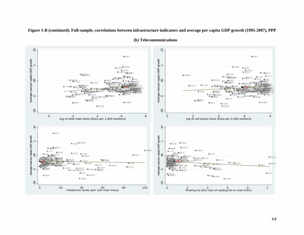
64
Figure 1-B (continued). Full-sample, correlations between infrastructure indicators and average per capita GDP growth (1995-2007), PPP
(b) Telecommunications
TCD
NERCAF
RWA
UGA
GINMDG
BDI
MOZ
TZA
COG
BGDBFA
AGO
CMR
ETH
MWI
MMR
MLI
KENZMBNGA
ERI
BEN
PNG
TGO
GHAMRT
LAO
HTICIV
NPLSENLSO
ZWE
GAB
PAKIDNPHL
SDNIND
NIC
PRY
MAR
LKAMNG
SWZ
YEMHND
CUB
BOL
PERKGZTHADZANAM
ALBBWA
VNM
DOM
ZAF
AZE
OMNECUGTM
PAN
GEO
KAZ
TUN
JAMSLVCOLSYRJORKWT
MYS
CHN
LBN
ROM
MEX
EGY
ARM
MDA
SAU
SVK
BRAARG
WBG
ARE
BIH
LTUTTO
CHLRUSUKR
LVA
URY
IRN
MKD
MUSCZE
BLR
EST
CRITUR
POL
PRT
PRISVN
NZL
HUNBGRNORSGP
JPN
ESPFIN
NLDAUT
HRVKOR
IRL
BELITA
HKGISRGBRAUSUSACANDNK
GRC
FRACHEDEUSWEEGY
-.05
0.0
5.1
.15
Ave
rage
real
per
cap
ita G
DP
gro
wth
0 2 4 6 8log of total main lines (lines per 1,000 workers)
MMR
ETH
PNGERI
NPL
CUB
TKM
BDI
NERCAF
TCD
RWA
GINMWIMDG
BGDUZBTJKBFA
GNBZWE
MOZ
LBR
MLIPAK
LAO
ZMB
UGA
LBY
HTI
SDN
TZA
AGO
INDVNM
KGZ
BEN
KHM
TGO
ARM
IRN
KEN
GHANGAYEMCMR
LSO
CIV
SENHND
COGGMB
LKA
IDNPER
SYR
EGY
KAZ
MNG
AZE
URYNIC
GEO
DZA
SWZ
MDA
NAM
CHN
MRTBOL
BLR
COLCRI
LBNECU
UKR
PRY
DOM
SLV
BIH
BRAARGTHAGTM
GAB
BWA
MARCANOMNPANPHLMEX
ALB
JOR
MUSROMTUNRUS
TTO
ZAFMKD
SAU
USATUR
WBG
MYS
POL
JPN
LVA
NZL
HRV
CHL
KWTCHE
BGR
ARE
KORSVK
AUSFRANLDDEUNOR
SVN
DNK
GRCPRI
PRT
SGPFIN
EST
JAM
IRL
ESPGBRAUTBEL
HUNCZE
LTU
SWEHKG
ITAISR
EGY
-.05
0.0
5.1
.15
Ave
rage
real
per
cap
ita G
DP
grow
th
0 2 4 6 8log of cell phone lines (lines per 1,000 workers)
JPNARE
SGPEGYHKG
KOR
MEXGINSAU
TWN
BRAOMNBGR
HNDKWT
CRIDZAPHLNIC
SDN
SEN
MDA
TGO
AUTTHA
PRY
IRL
BEL
BDI
BEN
CZEGBR
RUS
DNKESPCUBHUN
MKDAUSPRTJOR
LTULVA
GRC
SVK
USA
HRVPOL
EST
PANSVNROM
RWA
TUR
SLVECUIDN
BIH
GEO
NGAMRT
MNGTUNLKACHL
MARSYR
BLR
GHATZAMYS
COL
BFA
JAM
MUSUKRNAM
GAB
AZE
KAZ
ZAF
MDGCAF
ARM
ZWE
ERI
TCD
ALBMOZ
LSO
WBG
SWZ NER
NPLTKMCIV
ETHUZB
ZMBKEN
TJK
IND
MMR
EGY
-.05
0.0
5.1
.15
Ave
rage
real
per
cap
ita G
DP g
row
th
0 20 40 60 80 100Telephone faults (per 100 main lines)
CANAUSDNK
TWNFIN
DEUSWEHKG
JPNURY
KORHRV
NZL
SGP
ITACHENLDNORKWTFRAGBRAUTARE
MAR
SVNGRC
PNG
HUNCHLCZEPERJOROMNTUR
LTU
ZAFBRAARG
SVK
ECU
WBG
PANMYSCRIBOL
EST
MDG
NAM
LVA
UZB
PRYSAU
AZE
TJK
MUS
SLVSEN
IND
BGR
GIN
POL
CIV
TZAPAK
KAZ
EGYTUN
COLTHA
GAB
KGZIRN
BLR
BWA
ARM
ROM
TKMCAF
ZMB
GEO
RUSLAO
BFAMDA
MOZ
UKRMNG
BEN
BGD
MMR
GMB
LKA
MWIDZA
KEN
BDI
ALB
JAM
GNB
YEM
TGOSWZ
ETH
ZWE
GHALSONPL
ERI
SDN
HNDEGY
-.05
0.0
5.1
.15
Ave
rage
real
per
cap
ita G
DP g
row
th
0 .2 .4 .6 .8 1Waiting list (the ratio of waiting list to main lines)

65
Figure 1-B (continued). Full-sample, correlations between infrastructure indicators and average per capita GDP growth (1995-2007), PPP
(c) Electricity
KHM
TCD
RWA
TGO
WBGBDI
NERCAF
ETHUGA
MDG
BFA
ERI
GNB
BENGMB
TZA
MWISLESENNPLMLI
HTI
GIN
BGD
MMR
SDN
KENCOG
AGO
LSONGACMRGHAMRT
CIV
YEM
BWA
LBRVNM
PNG
IDN
MOZINDLAO
BOLNICPAK
ZWE
LKA
SWZ
ZMBNAMSLVPHLMARHNDPERDZAGTM
CHN
COLECUTHA
MNG
GAB
CUBEGYTUN
SYRBRA
CRIJORPANUZB
MEX
MUS
ALB
JAM
URY
TUR
AZE
DOM
TKM
IRNMDA
LBN
BLR
KGZCHL
ARG
POL
MKDMYS
GEO
HRVROM
LVA
HUN
PRTLBYZAFTJK
KAZ
BIH
GRC
TTO
UKR
ARE
KOR
NLDGBR
ARM
IRL
PRY
SVK
ITA
RUSSVN
DEU
CZE
BELESPHKGSGP
LTU
BGROMNAUT
PRI
ISRSAU
EST
NZLJPNFRACHE
AUSDNKUSA
FIN
CANKWT
SWENOREGY
-.05
0.0
5.1
.15
Ave
rage
real
per
cap
ita G
DP g
row
th
-6 -4 -2 0 2log of EGC (megawatts per 1,000 workers)
ISR
FINKORTWN
GTMZMB
PRY
NLD
SVK
DNKJPNBELAUTMYS
SVN
DEUFRA
TTO
SGPCZE
ZAFAUS
CHE
CHN
USACAN
ARE
LTU
ITA
SWE
SAU
THACHLNOR
IRL
GBRESPUZBGRC
PRT
POL
BGDPERETH
JAM
MOZBWA
VNM
CRIROM
EST
KWT
EGY
BLR
BOL
HUNTUNRUSBGRHKG
AZE
PHLSLVJORNZL
TKM
IDNBEN
AGO
SENGHATJKUKR
ZWE
LBNARG
TURCUBOMN
KAZ
GEO
SDN
CIV
BIH
MEX
ARM
DZAMAR
LKAHRV
BRA
IRNPAN
KENGAB
NAM
LVA
CMRCOLNPL
MMR
MKDYEMHNDTZA
SYR
NICPAK
IND
LBY
KGZURY
DOM
NGA
TGO
ALB
MDA
ECU
HTI
COG
EGY
-.05
0.0
5.1
.15
Aver
age
real
per
cap
ita G
DP
grow
th
0 20 40 60 80Power loss (% of total output)
TCD
DOM
UGA
ALB
BGD
BDI
NGATJK
MDG
TZA
NPL
ZWE
AGO
GMB
KHM
CMRMWIBEN
GEO
MRTNIC
MNG
BFA
ECUKEN
IND
PRY
LSOMLIKGZ
MOZ
HNDIDNMDA
VNM
PAKUKRETH
LKARUSROM
AZECHN
BOLARGPHL
BGR
ARM
MEXZAF
TUR
BIH
DZAMKD
KAZPOL
JAM
TTO
GTMCOL
PER
BWA
PAN
BRA
LVA
EGYNAMMARGRC
HRV
SLVNZL
LTU
HUN
ITA
CRIURYZMB
THATUN
EST
MUSCHLJOR
MYSPRT
SVNTWN
ESPAUS
IRL
KORCZE
SVK
USAKWTCANISRSWENORAUTAREBEL
SGPFINGBRHKGNLDCHEFRADEUJPNDNK
EGY
-.05
0.0
5.1
.15
Ave
rage
real
per
cap
ita G
DP g
rowth
0 2 4 6 8Quality of electricity supply
MOZ
BFA
MWI
UGATZALSO
MMR
KENMDG
ETH
AGO
TGOZMBCOG
KHM
ERI
BEN
KOR SDNBGD
NPLSEN
ZWE
NAM
HTI
YEM
BWA
NGACMR
GAB
GHA
CIV
IDNPAK
IND
HNDBOL
MNGLKA
NICZAF
PER
SLVPHL
VNM
MARPAN
PRY
COLJAM
SYRECUARE
DOMMUS
ARGURYOMNCUB
BRAISRSAULBY
IRNMYSEGYDZACRICHLTUNTHA
TTO
TWN
CHN
JORLBNKWT
SGPEGY
-.05
0.0
5.1
.15
Ave
rage
real
per
cap
ita G
DP g
row
th
0 20 40 60 80 100Access to Electricity (% of population)

66
Figure 1-B (continued). Full-sample, correlations between infrastructure indicators and average per capita GDP growth (1995-2007), PPP
(d) Water and Sanitation
PNG
ETH
NER
MOZ
MDG
NGATCD
AGO
SLE
TZA
KEN
GNB
HTI
ZMBTGOSWZ
LAO
MLIMRT
ERI
UGA
LBRRWAKHM
BEN
CAF
YEMTJKGINCMR
SDN
BDI
COG
BFA
MNG
MWI
PRY
SEN
AZE
LSONICGHA
MMR
BGD
IDN
ZWE
CIV
LKA
MARPERHNDSLVDZA
GMBBOL
GAB
ROM
CHN
UZB
IND
WBG
NPL
KGZ
SYRPAK
MDA
BRA
CUBPAN
VNM
ZAF
JAM
PHLNAMCOL
TUN
TTO
DOM
MEXECU
CHL
GTM
KAZ
ARG
BWA
UKR
ALB
RUSTURJOREGY
ARM
CRITHABGR
USA
BIH
PRT
HRV
GEO
MYS
LVA
HUN
AUSMUS
URYGBR
ARE
BLR
CHEDNKISRMKDAUTFRA
SVK
SWEFIN
JPN
ESPGRCCANDEU
SGP
EST
NLDLBN
CZENOR
EGY
-.05
0.0
5.1
.15
Aver
age
real
per
cap
ita G
DP
grow
th
20 40 60 80 100Access to Improved Water Source(% of population)
ERI
NER
TCDGHA
SLE
ETH
MDGTGO
BFA
HTI
GINCOG
RWA
CIV
MRTNPLSEN
INDKHM
BENNGA
MOZ
CAF
LBR
GNB
UGATZANAM
SDNBGD
GAB
LSO
BDI
KENBOL
PNG
MLIYEM
ZWE
BWALAO
NIC
SWZ
AGO
MNG
CMRIDN
GMBZMBPAKZAFMWI
VNM
CHN
EGYHND
PRY
MARPERROM
PAN
BRA
LVA
PHLCOL
MDADOM
AZE
WBG
MEX
MMR
JAMGTMECUJOR
TUN
SLV
LKARUSTUR
MKD
ARM
ARG
TTO
SYRTJKKGZUKR
GEO
BLR
CHLMUS
DZAMYS
BIH
EST
UZBTHACRI
ARELBY
ALBKAZ
CUBGRC
PRT
BGR
HRV
CZEESPAUSDNK
SGP
DEUURYCANUSA
HUN
NLDCHEJPN
SVK
SWEAUT
FINEGY
-.05
0.0
5.1
.15
Aver
age
real
per
cap
ita G
DP
gro
wth
0 20 40 60 80 100Access to Sanitation Facilities(% of population)

67
APPENDIX 3: Econometric Methodology
Although our focus is on the estimation of the growth effects of public
infrastructure, we must make sure that the full growth regression is correctly specified
and estimated. Thus, we need to ensure that all relevant variables are included, that their
potential endogeneity is controlled for, and that we account for unobserved effects.
The growth regression presented above poses some challenges for estimation. The
first is the presence of unobserved period- and country-specific effects. While the
inclusion of period-specific dummy variables can account for the time effects, the
common methods of dealing with country-specific effects (that is, within-group or
difference estimators) are inappropriate given the dynamic nature of the regression. The
second challenge is that most explanatory variables, including the public infrastructure
indices, are likely to be jointly endogenous with economic growth, so we need to control
for the biases resulting from simultaneous or reverse causation. The following outlines
the econometric methodology we use to control for country-specific effects and joint
endogeneity in a dynamic model of panel data.
We use the generalized method of moments (GMM) estimators developed for
dynamic models of panel data that were introduced by Holtz-Eakin, Newey, and Rosen
(1988), Arellano and Bond (1991), and Arellano and Bover (1995). These estimators are
based, first, on differencing regressions or instruments to control for unobserved effects
and, second, on using previous observations of explanatory and lagged-dependent
variables as instruments (which are called internal instruments).
After accounting for time-specific effects, we can rewrite equation 4.1:
tiitititi Xyy ,,1,, '
(4.2)
To eliminate the country-specific effect, we take first differences of equation 4.2:
y y y y X Xi t i t i t i t i t i t i t i t, , , , , , , ,' 1 1 2 1 1 (4.3)

68
The use of instruments is required to deal with the likely endogeneity of the
explanatory variables and the problem that, by construction, the new error term, i,t – i,t–1,
is correlated with the lagged dependent variable, yi,t–1 – yi,t–2. The instruments take
advantage of the panel nature of the data set in that they consist of previous observations
of the explanatory and lagged-dependent variables. Conceptually, this assumes that
shocks to economic growth (that is, the regression error term) be unpredictable given past
values of the explanatory variables. The method does allow, however, for current and
future values of the explanatory variables to be affected by growth shocks. It is this type
of endogeneity that the method is devised to handle.
Under the assumptions that the error term, , is not serially correlated and that the
explanatory variables are weakly exogenous (that is, the explanatory variables are
assumed to be uncorrelated with future realizations of the error term), our application of
the GMM dynamic panel estimator uses the following moment conditions:
E y for s t Ti t s i t i t, , , ; , ..., 1 0 2 3 (4.4)
E X for s t Ti t s i t i t, , , ; , ..., 1 0 2 3 (4.5)
for s ≥ 2 and t = 3,…, T. Although in theory the number of potential moment conditions
is large and growing with the number of time periods, T, when the sample size in the
cross-sectional dimension is limited, it is recommended to use a restricted set of moment
conditions in order to avoid overfitting bias (we return to this issue below). In our case,
we work with the first five acceptable lags as instruments.32 As mentioned above, the
indicator of natural disasters and the measure of external shocks (i.e. growth rate of terms
of trade) are treated as exogenous variables.
The GMM estimator based on the conditions in 4.4 and 4.5 is known as the
difference estimator. Notwithstanding its advantages with respect to simpler panel data
32 Specifically, regarding the difference regression corresponding to the periods t and t-1, we use the following instruments: for the variables measured as period averages --financial depth, government spending, trade openness, inflation, and crisis volatility-- the instrument corresponds to the average of period t-2; for the variables measured as initial values --per capita output and secondary school enrollment-- the instrument corresponds to the observation at the start of period t-1.

69
estimators, the difference estimator has important statistical shortcomings. Blundell and
Bond (1998) and Alonso-Borrego and Arellano (1999) show that when the explanatory
variables are persistent over time, lagged levels of these variables are weak instruments
for the regression equation in differences. Instrument weakness influences the
asymptotic and small-sample performance of the difference estimator toward inefficient
and biased coefficient estimates, respectively.33
To reduce the potential biases and imprecision associated with the difference
estimator, we use an estimator that combines the regression equation in differences and
the regression equation in levels into one system (developed in Arellano and Bover, 1995,
and Blundell and Bond, 1998). For the equation in differences, the instruments are those
presented above. For the equation in levels (equation 4.2), the instruments are given by
the lagged differences of the explanatory variables.34 These are appropriate instruments
under the assumption that the correlation between the explanatory variables and the
country-specific effect is the same for all time periods. That is,
qandpallforXEXE
andyEyE
iqtiipti
iqtiipti
][][
][][
,,
,,
(4.6)
Using this stationarity property and the assumption of exogeneity of future growth shocks,
the moment conditions for the second part of the system (the regression in levels) are
given by:
0 ][ ,2,1, tiititi yyE (4.7)
0 ][ ,2,1, tiititi XXE (4.8)
33 An additional problem with the simple difference estimator involves measurement error: differencing may exacerbate the bias stemming from errors in variables by decreasing the signal-to-noise ratio (see Griliches and Hausman, 1986). 34 The timing of the instruments is analogous to that used for the difference regression: for the variables measured as period averages, the instruments correspond to the difference between t-1 and t-2; and for the variables measured at the start of the period, the instruments correspond to the difference between t and t-1.

70
We thus use the moment conditions presented in equations 4.4, 4.5, 4.7, and 4.8
and employ a GMM procedure to generate consistent and efficient estimates of the
parameters of interest and their asymptotic variance-covariance (Arellano and Bond
1991; Arellano and Bover 1995). These are given by the following formulas:
yZZXXZZX 'ˆ')'ˆ'(ˆ 111 (4.9)
11 )'ˆ'()ˆ( XZZXAVAR (4.10)
where is the vector of parameters of interest (, ); y is the dependent variable stacked
first in differences and then in levels; X is the explanatory-variable matrix including the
lagged dependent variable (yt–1, X) stacked first in differences and then in levels; Z is the
matrix of instruments derived from the moment conditions; and ̂ is a consistent
estimate of the variance-covariance matrix of the moment conditions.35
Note that we use only a limited set of moment conditions. In theory the potential
set of instruments spans all sufficiently lagged observations and, thus, grows with the
number of time periods, T. However, when the sample size in the cross-sectional
dimension is limited, it is recommended to use a smaller set of moment conditions in
order to avoid over-fitting bias (see Arellano and Bond 1998; for a detailed discussion of
over-fitting bias in the context of panel-data GMM estimation, see Roodman 2007). This
is our case, and therefore we use two steps to limit the moment conditions. First, as
described in detail above, we use as instruments only five appropriate lags of each
endogenous explanatory variable. Second, we use a common variance-covariance of
moment conditions across periods. This results from substituting the assumption that the
average (across periods) of moment conditions for a particular instrument be equal to
zero for the assumption, conventional but more restrictive, that each of the period
moment conditions be equal to zero.36 At the cost of the reduced efficiency, our two
35 Arellano and Bond (1991) suggest the following two-step procedure to obtain consistent and efficient GMM estimates. First, assume that the residuals, i,t, are independent and homoskedastic both across countries and over time; this assumption corresponds to a specific weighting matrix that is used to produce first-step coefficient estimates. Second, construct a consistent estimate of the variance-covariance matrix of the moment conditions with the residuals obtained in the first step, and then use this matrix to re-estimate the parameters of interest (that is, second-step estimates). 36 This uses the “collapse” option of xtabond2 for STATA.

71
steps decrease over-fitting bias in the presence of small samples by accommodating cases
when the unrestricted variance-covariance is too large for estimation and inversion given
both a large number of explanatory variables and the presence of several time-series
periods.
The consistency of the GMM estimators depends on whether lagged values of the
explanatory variables are valid instruments in the growth regression. We address this
issue by considering a specification test. This is the Hansen test of overidentifying
restrictions, which tests the validity of the instruments by analyzing the sample analog of
the moment conditions used in the estimation process. Failure to reject the null
hypothesis gives support to the model.

72
APPENDIX 4: Infrastructure Investment – Recently Published Disaggregation Figure 4-A. Infrastructure Investment in Egypt (1983-2007)
(Percentage of GDP)
(d) Electricity
0.0
1.0
2.0
3.0
4.0
5.0
6.0
1983 1987 1991 1995 1999 2003 2007
Public Private
(b) Transportation (incl. SC)
0.01.02.03.04.05.06.07.08.0
1983 1987 1991 1995 1999 2003 2007
(a) Total Investment
0.0
2.0
4.0
6.0
8.0
10.0
12.0
14.0
1983 1987 1991 1995 1999 2003 2007
(c) Communications
0.0
0.2
0.4
0.6
0.8
1.0
1.2
1.4
1983 1987 1991 1995 1999 2003 2007

73
APPENDIX 5: Additional Regression Analysis on Infrastructure Expenditure and Improvement
Table 6-A. Electricity Expenditure and Improvement
ElectricityEstimation Method: Quantile regression
Ratio of expenditure to labor force 0.010 ***(expenditure on electricity per 100,000 workers) [6.02]
Ratio of expenditure to labor force 0.112 ***(expenditure on electricity per 100,000 workers, in logs) [4.13]
Ratio of expenditure to GDP 0.007 ***(expenditure on electricity / 1,000 GDP) [6.38]
Ratio of expenditure to GDP 0.129 ***(expenditure on electricity / 1,000 GDP, in logs) [6.24]
Initial value of infrastructure index -0.232 ** -0.542 ** -0.226 ** -0.687 ***[2.43] [2.06] [2.22] [2.76]
Initial value of infrastructure index * Expenditure 0.009 0.184 * 0.010 * 0.219 **[1.43] [1.82] [1.99] [2.61]
Constant -0.135 *** -0.281 *** -0.145 *** -0.372 ***[5.05] [3.87] [5.83] [6.11]
Observations 34 34 34 34R-squared 0.46 0.35 0.47 0.42
Notes:The dependent variable and initial value of index are smoothed by using the Hodrik Prescott filter.All the expenditure variables are the moving average of expenditures in the last three years.Numbers in brackets are the corresponding t-statistics.
* significant at 10%; ** significant at 5%; *** significant at 1%
Dependent variable: Change in Electricity Infrastructure Index
[4][1] [2] [3]
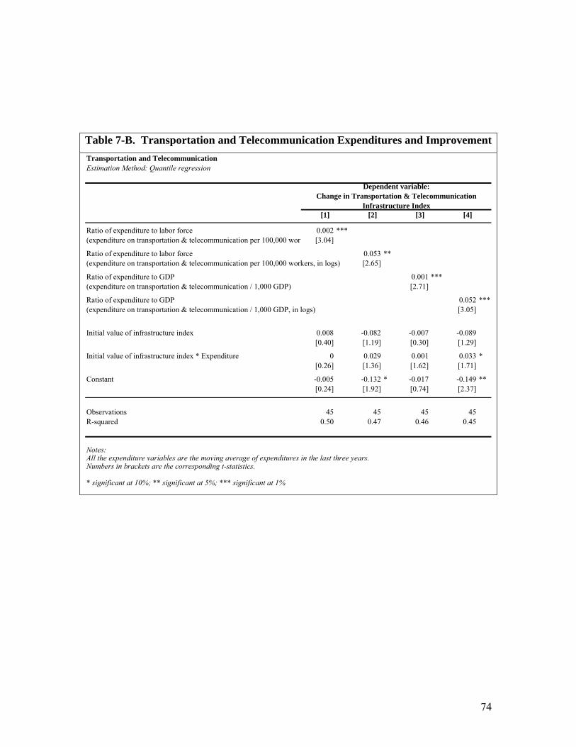
74
Table 7-B. Transportation and Telecommunication Expenditures and Improvement
Transportation and TelecommunicationEstimation Method: Quantile regression
Ratio of expenditure to labor force 0.002 ***(expenditure on transportation & telecommunication per 100,000 work [3.04]
Ratio of expenditure to labor force 0.053 **(expenditure on transportation & telecommunication per 100,000 workers, in logs) [2.65]
Ratio of expenditure to GDP 0.001 ***(expenditure on transportation & telecommunication / 1,000 GDP) [2.71]
Ratio of expenditure to GDP 0.052 ***(expenditure on transportation & telecommunication / 1,000 GDP, in logs) [3.05]
Initial value of infrastructure index 0.008 -0.082 -0.007 -0.089[0.40] [1.19] [0.30] [1.29]
Initial value of infrastructure index * Expenditure 0 0.029 0.001 0.033 *[0.26] [1.36] [1.62] [1.71]
Constant -0.005 -0.132 * -0.017 -0.149 **[0.24] [1.92] [0.74] [2.37]
Observations 45 45 45 45R-squared 0.50 0.47 0.46 0.45
Notes:All the expenditure variables are the moving average of expenditures in the last three years.Numbers in brackets are the corresponding t-statistics.
* significant at 10%; ** significant at 5%; *** significant at 1%
Dependent variable: Change in Transportation & Telecommunication
Infrastructure Index[4][1] [2] [3]