Information Networks

Failures and Epidemics in Networks

Lecture 12

Spread in Networks

Understanding the spread of viruses (or rumors, information, failures etc) is one of the driving forces behind network analysis predict and prevent epidemic outbreaks (e.g. the

SARS outbreak) protect computer networks (e.g. against worms) predict and prevent cascading failures (U.S. power

grid) understanding of fads, rumors, trends

• viral marketing anti-terrorism?

Percolation in Networks

Site Percolation: Each node of the network is randomly set as occupied or not-occupied. We are interested in measuring the size of the largest connected component of occupied vertices

Bond Percolation: Each edge of the network is randomly set as occupied or not-occupied. We are interested in measuring the size of the largest component of nodes connected by occupied edges

Good model for failures or attacks

Percolation Threshold

How many nodes should be occupied in order for the network to not have a giant component? (the network does not percolate)

Percolation Threshold for the configuration model

If pk is the fraction of nodes with degree k, then if a fraction q of the nodes is occupied, the probability of a node to have degree m is

This defines a new configuration model apply the known threshold

For scale free graphs we have qc ≤ 0 for power law exponent less than 3! there is always a giant component (the network

always percolates)

mkm

mkkm q1q

m

kp'p

Percolation threshold

An analysis for general graphs is and general occupation probabilities is possible for scale free graphs it yields the same results

But … if the nodes are removed preferentially (according to degree), then it is easy to disconnect a scale free graph by removing a small fraction of the edges

Network resilience

Scale-free graphs are resilient to random attacks, but sensitive to targeted attacks. For random networks there is smaller difference between the two

Real networks

Cascading failures

Each node has a load and a capacity that says how much load it can tolerate.

When a node is removed from the network its load is redistributed to the remaining nodes.

If the load of a node exceeds its capacity, then the node fails

Cascading failures: example

The load of a node is the betweeness centrality of the node

The capacity of the node is C = (1+b)L the parameter b captures the additional load a

node can handle

Cascading failures in SF graphs

The SIR model

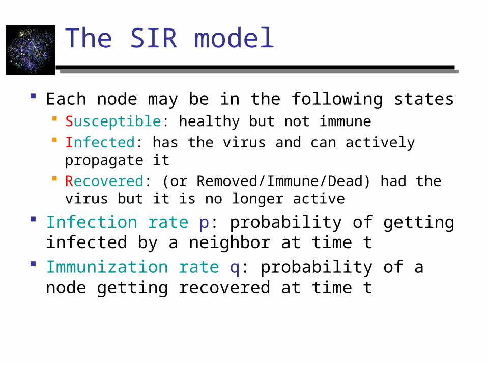
Each node may be in the following states Susceptible: healthy but not immune Infected: has the virus and can actively propagate it Recovered: (or Removed/Immune/Dead) had the

virus but it is no longer active

Infection rate p: probability of getting infected by a neighbor per unit time

Immunization rate q: probability of a node getting recovered per unit time

The SIR model

It can be shown that virus propagation can be reduced to the bond-percolation problem for appropriately chosen probabilities again, there is no percolation threshold for

scale-free graphs

A simple SIR model

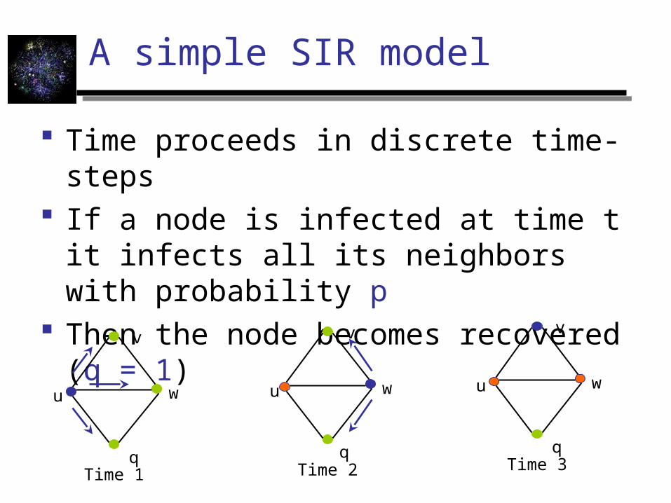
Time proceeds in discrete time-steps If a node is infected at time t it infects all

its neighbors with probability p Then the node becomes recovered (q = 1)

u

v

w

qTime 3

u

v

w

qTime 1

u

v

w

qTime 2

The caveman small-world graphs

The SIS model

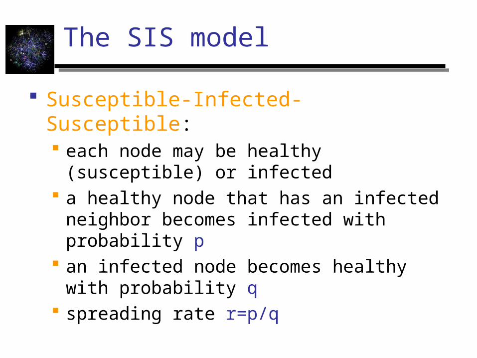
Susceptible-Infected-Susceptible: each node may be healthy (susceptible) or

infected a healthy node that has an infected neighbor

becomes infected with probability p an infected node becomes healthy with

probability q spreading rate r=p/q

Epidemic Threshold

The epidemic threshold for the SIS model is a value rc such that for r < rc the virus dies out, while for r > rc the virus spreads.

For homogeneous graphs,

For scale free graphs

For exponent less than 3, the variance is infinite, and the epidemic threshold is zero

2ck

kr

k1

rc

An eigenvalue point of view

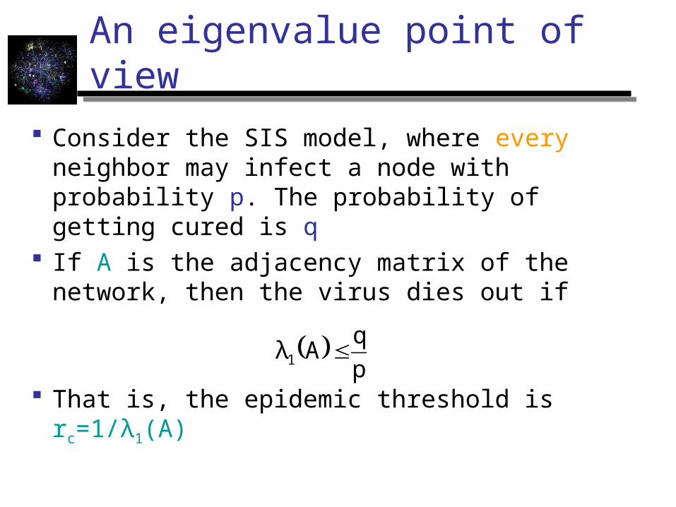
Consider the SIS model, where every neighbor may infect a node with probability p. The probability of getting cured is q

If A is the adjacency matrix of the network, then the virus dies out if

That is, the epidemic threshold is rc=1/λ1(A)

pq

Aλ1

Information Networks

Virus propagation, Immunization and Gossip

Lecture 13

Percolation in Networks

Site Percolation: Each node of the network is randomly set as occupied or not-occupied. We are interested in measuring the size of the largest connected component of occupied vertices

Bond Percolation: Each edge of the network is randomly set as occupied or not-occupied. We are interested in measuring the size of the largest component of nodes connected by occupied edges

Good model for failures or attacks

Network resilience

Scale-free graphs are resilient to random attacks, but sensitive to targeted attacks. For random networks there is smaller difference between the two

The SIR model

Each node may be in the following states Susceptible: healthy but not immune Infected: has the virus and can actively propagate it Recovered: (or Removed/Immune/Dead) had the

virus but it is no longer active

Infection rate p: probability of getting infected by a neighbor at time t

Immunization rate q: probability of a node getting recovered at time t

The SIS model

Susceptible-Infected-Susceptible: each node may be healthy (susceptible) or

infected a healthy node that has an infected neighbor

becomes infected with probability p an infected node becomes healthy with

probability q spreading rate r=p/q

Epidemic Threshold

The epidemic threshold for the SIS model is a value rc such that for r < rc the virus dies out, while for r > rc the virus spreads.

For homogeneous graphs,

For scale free graphs

For exponent less than 3, the variance is infinite, and the epidemic threshold is zero

2ck

kr

k1

rc

An eigenvalue point of view

Time proceeds in discrete timesteps. At time t, an infected node u infects a healthy neighbor v with

probability p. node u becomes healthy with probability q

If A is the adjacency matrix of the network, then the virus dies out if

That is, the epidemic threshold is rc=1/λ1(A)

pq

Aλ1

Multiple copies model

Each node may have multiple copies of the same virus v: state vector

• vi : number of virus copies at node i

At time t = 0, the state vector is initialized to v0

At time t,For each node i

For each of the vit virus copies at node i

the copy is propagated to a neighbor j with prob pthe copy dies with probability q

Analysis

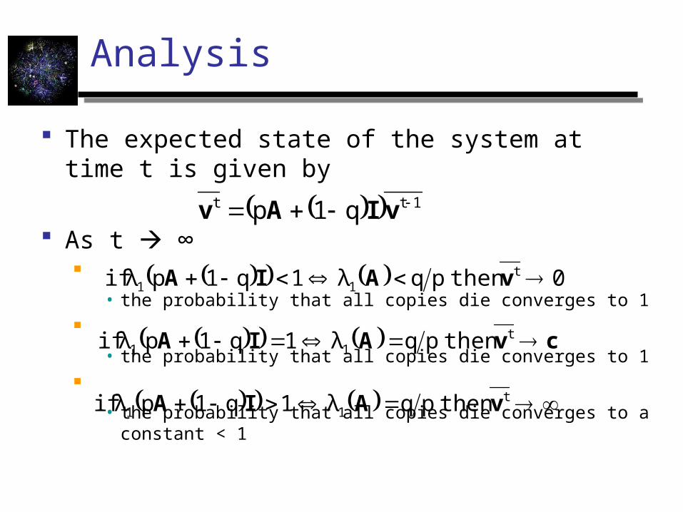
The expected state of the system at time t is given by

As t ∞

• the probability that all copies die converges to 1

• the probability that all copies die converges to 1

• the probability that all copies die converges to a

constant < 1

1tt vIAv q1p

0 then pqλ1q1p λif t11 vAIA

cvAIA t11 then pqλ1q1p λif

t11 then pqλ1q1p λif vAIA

Immunization

Given a network that contains viruses, which nodes should we immunize in order to contain the spread of the virus?

The flip side of the percolation theory

Immunization of SF graphs

Uniform immunization vs Targeted immunization

Immunizing aquaintances

Pick a fraction f of nodes in the graph, and immunize one of their acquaintances you should gravitate towards nodes with high

degree

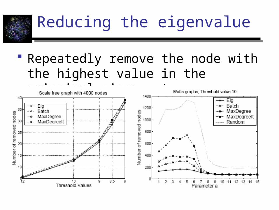
Reducing the eigenvalue

Repeatedly remove the node with the highest value in the principal eigenvector

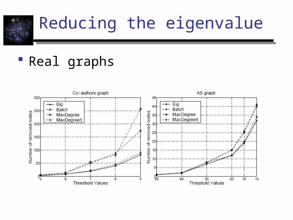
Reducing the eigenvalue

Real graphs

Gossip

Gossip can also be thought of as a virus that propagates in a social network.

Understanding gossip propagation is important for understanding social networks, but also for marketing purposes

Provides also a diffusion mechanism for the network

Independent cascade model

Each node may be active (has the gossip) or inactive (does not have the gossip)

Time proceeds at discrete time-steps. At time t, every node v that became active in time t-1 actives a non-active neighbor w with probability puw. If it fails, it does not try again the same as the simple SIR model

A simple SIR model

Time proceeds in discrete time-steps If a node u is infected at time t it infects

neighbor v with probability puv

Then the node becomes recovered (q = 1)

u

v

w

qTime 3

u

v

w

qTime 1

u

v

w

qTime 2

Linear threshold model

Each node may be active (has the gossip) or inactive (does not have the gossip)

Every directed edge (u,v) in the graph has a weight buv, such that

Each node u has a threshold value Tu (set uniformly at random)

Time proceeds in discrete time-steps. At time t an inactive node u becomes active if

1bu ofneighbor a isv

uv

uu ofneighbor active an isv

vu Tb

Influence maximization

Influence function: for a set of nodes A (target set) the influence s(A) is the expected number of active nodes at the end of the diffusion process if the gossip is originally placed in the nodes in A.

Influence maximization problem [KKT03]: Given an network, a diffusion model, and a value k, identify a set A of k nodes in the network that maximizes s(A).

The problem is NP-hard

Submodular functions

Let f:2UR be a function that maps the subsets of universe U to the real numbers

The function f is submodular if

when the principle of diminishing returns

TfvTfSfvSf

TS

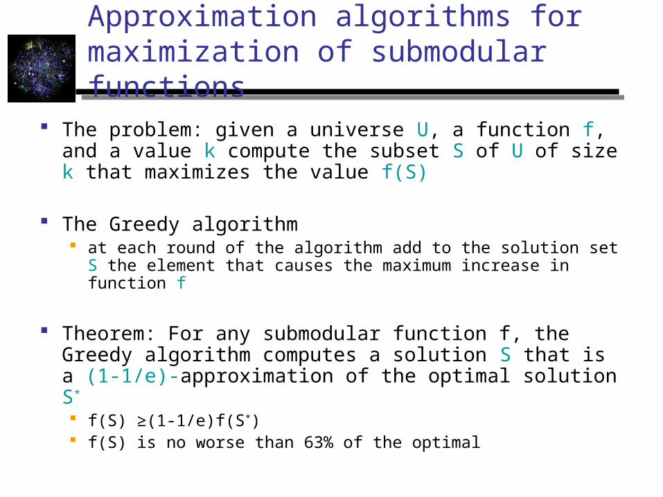
Approximation algorithms for maximization of submodular functions

The problem: given a universe U, a function f, and a value k compute the subset S of U of size k that maximizes the value f(S)

The Greedy algorithm at each round of the algorithm add to the solution set S the

element that causes the maximum increase in function f

Theorem: For any submodular function f, the Greedy algorithm computes a solution S that is a (1-1/e)-approximation of the optimal solution S*

f(S) ≥(1-1/e)f(S*) f(S) is no worse than 63% of the optimal

Submodularity of influence

How do we deal with the fact that influence is defined as an expectation?

Express s(A) as an expectation over the input rather than the choices of the algorithm

Independent cascade model

Each edge (u,v) is considered only once, and it is “activated” with probability puv.

We can assume that all random choices have been made in advance generate a subgraph of the input graph where edge (u,v) is

included with probability puv

propagate the gossip deterministically on the input graph the active nodes at the end of the process are the nodes

reachable from the target set A The influence function is obviously submodular when

propagation is deterministic The weighted combination of submodular functions is

also a submodular function

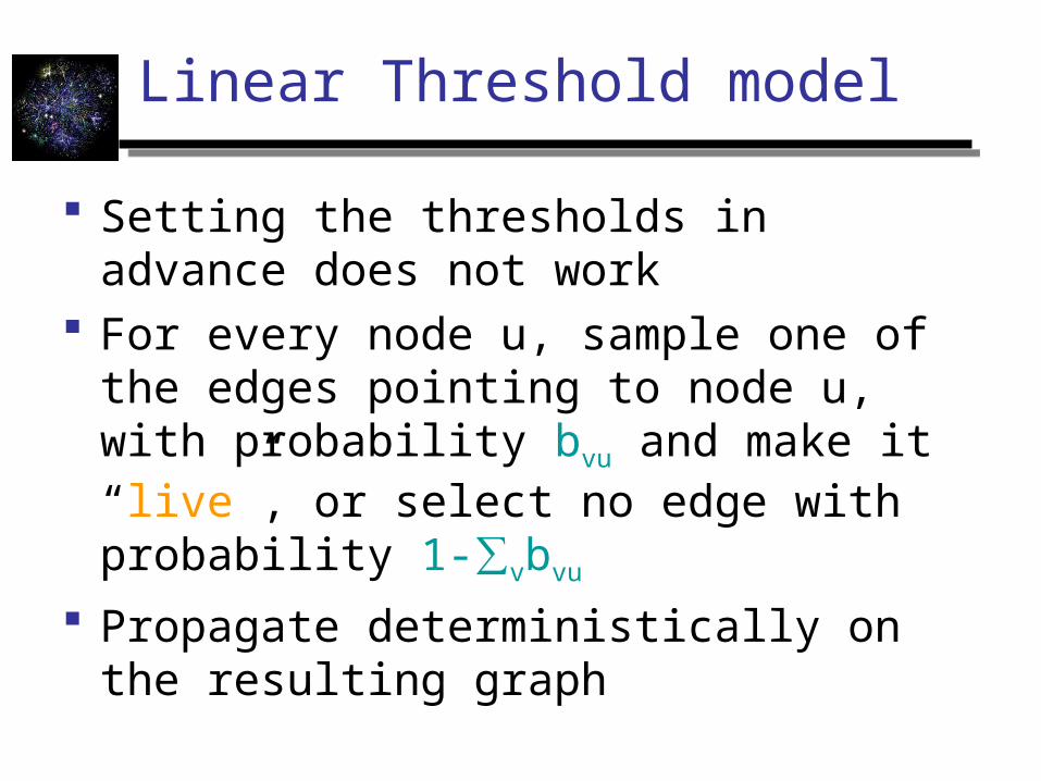
Linear Threshold model

Setting the thresholds in advance does not work

For every node u, sample one of the edges pointing to node u, with probability bvu and make it “live”, or select no edge with probability 1-∑vbvu

Propagate deterministically on the resulting graph

Model equivalence

For a target set A, the following two distributions are equivalent The distribution over active sets obtained by

running the Linear Threshold model starting from A

The distribution over sets of nodes reachable from A, when live edges are selected as previously described.

Simple case: DAG

Compute the topological sort of the nodes in the graph and consider them in this order.

If Si neighbors of node i are active then the probability that it becomes active is

This is also the probability that one of the nodes in Si is sampled

Proceed inductively

iSj

jib

General graphs

Let At be the set of active nodes at the end of the t-th iteration of the algorithm

Prob that inactive node v becomes active at time t, given that it has not become active so far, is

1t

1tt

Au uv

AAu uv

b1

b

General graphs

Starting from the target set, at each step we reveal the live edges from reachable nodes

Each live edge is revealed only when the source of the link becomes reachable

The probability that node v becomes reachable at time t, given that it was not reachable at time t-1 is the probability that there is an live edge from the set At – At-1

1t

1tt

Au uv

AAu uv

b1

b

Experiments

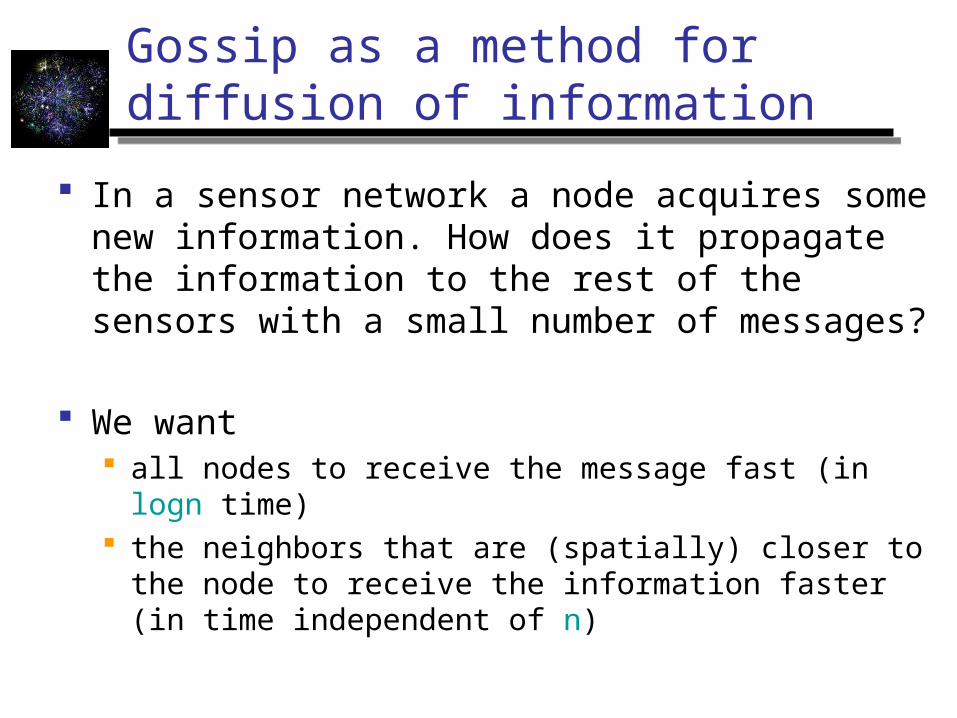
Gossip as a method for diffusion of information

In a sensor network a node acquires some new information. How does it propagate the information to the rest of the sensors with a small number of messages?

We want all nodes to receive the message fast (in logn time) the neighbors that are (spatially) closer to the node to

receive the information faster (in time independent of n)

Information diffusion algorithms

Consider points on a lattice

Randomized rumor spreading: at each round each node sends the message to a node chosen uniformly at random time to inform all nodes O(logn) same time for a close neighbor to receive the message

Neighborhood flooding: a node sends the message to all of its neighbors, one at the time, in a round robin fashion a node at distance d receives the message in time O(d) time to inform all nodes is O(√n)

Spatial gossip algorithm

At each round, each node u sends the message to the node v with probability proportional to duv

-Dr, where D is the dimension of the lattice and 1 < r < 2

The message goes from node u to node v in time logarithmic in duv. On the way it stays within a small region containing both u and v

References

M. E. J. Newman, The structure and function of complex networks, SIAM Reviews, 45(2): 167-256, 2003

R. Albert and L.A. Barabasi, Statistical Mechanics of Complex Networks, Rev. Mod. Phys. 74, 47-97 (2002).

Y.-C. Lai, A. E. Motter, T. Nishikawa, Attacks and Cascades in Complex Networks, Complex Networks, Springer Verlag

D.J. Watts. Networks, Dynamics and Small-World Phenomenon, American Journal of Sociology, Vol. 105, Number 2, 493-527, 1999

R. Pastor-Satorras and A. Vespignani, Epidemics and immunization in scale-free networks. In "Handbook of Graphs and Networks: From the Genome to the Internet", eds. S. Bornholdt and H. G. Schuster, Wiley-VCH, Berlin, pp. 113-132 (2002)

R. Cohen, S. Havlin, D. Ben-Avraham,Efficient Immunization Strategies for Computer Networks and Populations Phys Rev Lett. 2003 Dec 12;91(24):247901. Epub 2003 Dec 9

Y.ang Wang, Deepayan Chakrabarti, Chenxi Wang, Christos Faloutsos, Epidemic Spreading in Real Networks: An Eigenvalue Viewpoint, SDRS, 2003

D. Kempe, J. Kleinberg, E. Tardos. Maximizing the Spread of Influence through a Social Network. Proc. 9th ACM SIGKDD Intl. Conf. on Knowledge Discovery and Data Mining, 2003. (In PDF.)

D. Kempe, J. Kleinberg, A. Demers. Spatial gossip and resource location protocols. Proc. 33rd ACM Symposium on Theory of Computing, 2001