Information and Computation 247 (2016) 278–289

Contents lists available at ScienceDirect

Information and Computation

www.elsevier.com/locate/yinco

Approximate matching between a context-free grammar and

a finite-state automaton ✩

Sang-Ki Ko a, Yo-Sub Han a,∗, Kai Salomaa b

a Department of Computer Science, Yonsei University, Seoul 120-749, Republic of Koreab School of Computing, Queen’s University, Kingston, Ontario K7L 3N6, Canada

a r t i c l e i n f o a b s t r a c t

Article history:Received 6 October 2014Received in revised form 29 July 2015Available online 8 February 2016

Keywords:Approximate matchingEdit-distanceGap penaltyContext-free grammarsFinite-state automata

For a given context-free grammar (CFG) and a finite-state automaton (FA), we tackle the edit-distance problem—the problem of computing the most similar pair of strings in the two respective languages. In particular, we consider three different gap cost models for the edit-distance that are crucial for finding a proper alignment between two bio sequences: the linear, affine and concave models. We design efficient algorithms for the edit-distance between a CFG and an FA under these gap cost models. The time complexity of our algorithm for computing the linear or affine gap distance is polynomial and the time complexity for the concave gap distance is exponential.

© 2016 Elsevier Inc. All rights reserved.

1. Introduction

Given a pattern w and a text T , the string matching problem is to find occurrences of w in T and the approximate matching problem is to find occurrences of w ′ in T such that w and w ′ are similar by a predefined similarity metric. The most common similarity metric is the edit-distance [14]. Many researchers investigated the approximate pattern matching problem with various types of mismatches [1,6,15,16,18,23]. For example, Aho and Peterson [1], and Lyon [15] developed an O (m2n3) algorithm for the approximate matching between a string of length n and a context-free language specified by a grammar of size m. They generalized Earley’s algorithm [6] for parsing context-free languages and considered the edit-distance model [14] with a unit-cost function. Myers [18] considered several variants of the problem under various gap cost functions such as the linear, affine and concave gap costs; these gap cost models are important for identifying proper alignments between two bio sequences in practice [19,20]. Myers designed O (mn2(n + log m)) algorithms for the linear and the affine gap costs and sketched an O (m5n88m) algorithm for the concave gap cost.

The approximate matching problem is based on the edit-distance between two strings, or between a string and a lan-guage. This led researchers to examine the edit-distance between two formal languages. Mohri [17] proved that computing the edit-distance between two context-free languages is undecidable and provided a quadratic time algorithm for computing the edit-distance between two regular languages. Choffrut and Pighizzini [5] considered the relative edit-distance between languages and the reflexivity of binary relations. Konstantinidis [13] considered the edit-distance of a regular language—the minimum edit-distance among all pairs of distinct strings of the language. Recently, the authors [9] studied the Levenshtein distance [14] between a context-free language and a regular language given, respectively, by a pushdown automaton (PDA) P

✩ A preliminary version appeared in Proceedings of the 18th International Conference on Implementation and Application of Automata, CIAA 2013, LNCS 7982, 146–157, Springer-Verlag, 2013.

* Corresponding author.E-mail addresses: narame7@yonsei.ac.kr (S.-K. Ko), emmous@yonsei.ac.kr (Y.-S. Han), ksalomaa@cs.queensu.ca (K. Salomaa).

http://dx.doi.org/10.1016/j.ic.2016.02.0010890-5401/© 2016 Elsevier Inc. All rights reserved.

S.-K. Ko et al. / Information and Computation 247 (2016) 278–289 279

and a finite-state automaton (FA) A. Their algorithm constructs an alignment PDA that computes all possible alignments be-tween L(A) and L(P ), converts the alignment PDA into a CFG and finds the optimal alignment from the resulting grammar. Under the assumption that a PDA can push at most two symbols and pop at most one symbol, it takes O (n3) time to convert a PDA of size n into a CFG and the size of the resulting grammar is at most O (n3) [10]. If a context-free language is given by a CFG instead of a PDA, then we need to construct a PDA for an input CFG before computing the alignment PDA. This leads us to design algorithms that compute the edit-distance between a CFG and an FA without constructing a PDA, and to extend this problem to considering the approximate matching between a CFG and an FA.

We calculate the minimum edit-distance and the optimal alignment between the most similar pair of strings generated, respectively, by a CFG and an FA. We present algorithms for computing optimal alignments between a CFG and an FA under various gap distances. While several previous algorithms for the edit-distance between two formal languages are based on the Cartesian product construction [9,11,13,17], we design dynamic programming algorithms for the considered problem. Assume that the size of the input CFG is m and the size of the input FA is n. Our algorithms compute the linear and the affine gap distances in O (m2n5) time, and the concave gap distance in O (m5n88m log3 n) time.

In Section 2, we briefly recall basic notation and terminology. We define the edit-distance model in Section 3. In Sec-tion 4, we introduce a dynamic programming algorithm for computing the edit-distance between a CFG and an FA. The next two sections then extend the algorithm to the problems of computing the affine and the concave gap distances.

2. Preliminaries

In the following, � is always a finite alphabet of characters and �∗ denotes the set of all strings over �. The size |�| of � is the number of characters in �. A language over � is any subset of �∗ . Given a set X , 2X denotes the power set of X .

The symbol ∅ denotes the empty language and the symbol λ denotes the null string. The length of a string w ∈ �∗ is |w|. Given a string w ∈ �∗ , let w[i] be the i’th character of w and w[i, j] be the substring of w from w[i] to w[ j]—w[i, j] =w[i]w[i + 1] · · · w[ j]—where 1 ≤ i < j ≤ |w|. A (nondeterministic) finite-state automaton (FA) is specified by a tuple M =(Q , �, δ, s, F ), where Q is a finite set of states, � is an input alphabet, δ : Q × � → 2Q is a set-valued transition function, s ∈ Q is the start state and F ⊆ Q is a set of final states. If F consists of a single state f , we use f instead of { f } for short. We let Mq,p = (Q , �, δ, q, p) denote the new FA obtained from M by replacing the start state with q and the only final state with p.

The transition function δ is extended in the natural way to a function Q × �∗ → 2Q that reflects state changes on a sequence of characters. A string x over � is accepted by M if there is a labeled path from s to a state in F such that this path spells out the string x. In other words, δ(s, x) ∩ F = ∅. The language L(M) of M is the set of all accepted strings. Let |Q | be the number of states in M and |δ| be the number of transitions in M . We define the size |M| of M to be |Q | + |δ|.

A context-free grammar (CFG) G is specified by a tuple G = (V , �, R, S), where V is a set of variables, R ⊆ V × (V ∪�)∗is a finite set of productions and S ∈ V is the start symbol. Let αAβ be a string over V ∪ �, where A is a variable in V and A → γ is a production of G . Then, we say that αγ β is obtained from αAβ in a single derivation step and this is denoted by αAβ ⇒ αγ β . The reflexive, transitive closure of ⇒ is ∗⇒. The context-free language defined by G is L(G) = {w ∈ �∗ |S

∗⇒ w}. We say that a variable A ∈ V is useless if a CFG G A = (V , �, R, A)—A is the start symbol in G—generates the empty language. Note that we assume that a CFG has no useless variables. By the size |G| of the grammar G we mean the sum ∑

A→α∈R(1 + |α|) of the lengths of all productions of G .A CFG is in Chomsky normal form (CNF) if all of its production rules are of the form: A → BC or A → a, where

A, B, C ∈ V and a ∈ �. Every context-free grammar G generating a language not containing the null string can be converted into an equivalent CNF grammar of size O (|G|2).

We also consider pseudo-CNF grammars that in addition to the above rules allow rules of the form A → B , where A, B ∈ V . It is known that an arbitrary grammar G can be transformed into an equivalent pseudo-CNF grammar whose size is still O (|G|) [21].

For more details on automata theory, we refer the reader to the textbooks [10,24].

3. Edit-distance

The edit-distance between two strings x and y is the smallest number of atomic operations that transform x to y. Researchers considered different atomic edit operations in different applications in the literature [4,22]. Here we consider three basic operations—insertion, deletion and substitution—for simplicity. Given an alphabet �, let

� = {(a → b) | a,b ∈ � ∪ {λ},a = b implies a = λ}be a set of edit operations. Namely, � is an alphabet of all edit operations for deletions (a → λ), insertions (λ → a) and substitutions (a → b).

Let h be the morphism from �∗ into �∗ × �∗ defined by setting

h((a1 → b1) · · · (an → bn)) = (a1 · · ·an,b1 · · ·bn).

We say that ω ∈ �∗ is an alignment of strings x, y ∈ �∗ if h(ω) = (x, y). For example, a string ω = (a → λ)(b → b)(λ →c)(c → c) over � is an alignment between abc and bcc, and h(ω) = (abc, bcc). We associate a non-negative edit cost

280 S.-K. Ko et al. / Information and Computation 247 (2016) 278–289

c(σ ) to each edit operation σ ∈ �, where c is a function � → R+ . We can extend the function to give the cost of an alignment ω = σ1 · · ·σn , where σi ∈ �, 1 ≤ i ≤ n, in the natural way:

c(ω) =n∑

i=1

c(σi).

Definition 1. The edit-distance d(x, y) of two strings x and y is the minimal cost of an alignment ω between x and y:

d(x, y) = min{c(ω) | h(ω) = (x, y)}.We say that ω is optimal if d(x, y) = c(ω).

We simply denote the cost c(σ ) of an individual edit operation σ = (a → b) by c(a, b) instead of c((a → b)), where a, b ∈ � ∪{λ}. We assume that the cost function c satisfies two conditions: c(a, b) = c(b, a) and c(a, a) = 0, for a, b ∈ � ∪{λ}. We extend the definition of edit-distance for languages as follows:

Definition 2. The edit-distance d(L, R) between two languages L, R ⊆ �∗ is the minimum edit-distance of two strings, one is from L and the other is from R:

d(L, R) = min{d(x, y) | x ∈ L and y ∈ R}.

The edit-distance in Definition 2 is the distance between the closest pair of strings from, respectively, L and R , where the distance is measured based on the cost of the edit operations. In other words, the most similar pair of strings from two languages defines the edit-distance between the languages.

4. Main algorithm

We compute the edit-distance between two languages defined by a CFG and an FA. We assume that an input CFG G = (V , �, R, S) is in pseudo-CNF. We use a pseudo-CNF grammar (instead of a CNF grammar) because an arbitrary CFG can be converted to a pseudo-CNF grammar with only linear increase in size [21].

The main idea of our algorithm is to compute the edit-distance between two languages, where one language is a set of strings derived from a variable of the CFG and the other language is a set of strings spelled out by paths of the FA. We compute distances for all variables of the CFG and all pairs of states of the FA. Note that this approach is similar to the procedure for constructing a CFG that generates the intersection of the languages generated by a CFG and an FA [2].

Given a variable A ∈ V and two states p and q of Q , let C(A, q, p) be the minimum edit-distance between two strings xand y, where A ∗⇒ x and y is spelled out by a computation from q to p. Namely,

C(A,q, p) = min{d(v, w) | v ∈ L(G A) and w ∈ L(Mq,p)},where G A = (V , �, R, A) and Mq,p = (Q , �, δ, q, p). Then, min{C(S, s, f ) | f ∈ F } is the edit-distance between L(G) and L(M). In Lemma 3, we provide a recurrence for computing the C-values.

For a variable A ∈ V and states q, p ∈ Q , we define:

(i) X(A, q, p) = min{C(B, q, r) + C(D, r, p) | r ∈ Q , A → B D ∈ R},(ii) Y (A, q, p) = min{C(B, q, p) | A → B ∈ R}, and(iii) Z(A, q, p) = min{d(a, w) | A → a ∈ R, w ∈ L(Mq,p)}.

Lemma 3. For all variables A ∈ V of a CFG and states q, p ∈ Q of an FA,

C(A,q, p) = min{X(A,q, p), Y (A,q, p), Z(A,q, p)}. (1)

Proof. First we show that C(A, q, p) is not greater than the right-hand side in Equation (1).

(i) Suppose that the following conditions hold:• B ∗⇒ t and D ∗⇒ u, where t, u ∈ �∗ ,• r ∈ δ(q, w) and p ∈ δ(r, w ′), where w, w ′ ∈ �∗ , and• C(B, q, r) = d(t, w) and C(D, r, p) = d(u, w ′).If A → B D ∈ R , then A ∗⇒ tu. We also have p ∈ δ(q, w w ′). Therefore,

C(A,q, p) ≤ d(tu, w w ′) ≤ d(t, w) + d(u, w ′) = C(B,q, r) + C(D, r, p).

(ii) If A → B ∈ R , then it follows that C(A, q, p) ≤ C(B, q, p).

S.-K. Ko et al. / Information and Computation 247 (2016) 278–289 281

(iii) If A → a ∈ R for a ∈ � and p ∈ δ(q, w), then a ∈ L(G A) and C(A, q, p) ≤ d(a, w) because C(A, q, p) is the minimum of a set that contains d(a, w).

Hence C(A, q, p) is less than or equal to every term in the right-hand side in Equation (1). Next, we prove that C(A, q, p)

is no less than the right-hand side. Assume that C(A, q, p) = d(v, w), where A ∗⇒ v and p ∈ δ(q, w). Since the input CFG is in pseudo-CNF, there are three possible cases in which the derivation A ∗⇒ v can begin:

(i) A ⇒ B D ∗⇒ v ,(ii) A ⇒ B ∗⇒ v ,(iii) A ⇒ a = v .

In the first case, v is defined as tu where B ∗⇒ t and D ∗⇒ u. It follows that for some 1 ≤ k ≤ |w| we have

C(A,q, p) = d(v, w) = d(t, w[1,k]) + d(u, w[k + 1, |w|]) ≥ C(B,q, r) + C(D, r, p),

where r ∈ δ(q, w[1, k]) and p ∈ δ(r, w[k + 1, |w|]). Similarly in case (ii) it is easy to verify that C(A, q, p) ≥ C(B, q, p) and in case (iii) that C(A, q, p) ≥ d(a, w). �

Note that Equation (1) is an essential recurrence equation for computing d(L(G), L(M)) in a bottom-up dynamic pro-gramming approach. We first compute the third term Z(A, q, p)—the case when there exists a production rule A → a ∈ R—in Equation (1) since it is independent from the other terms.

We use Z -values to store Z -values temporarily. After updating all Z -values by considering all possible cases, we set Z -values as the final Z -values.

Initially, we set

Z(A,q, p) = min{c(a,b), c(a, λ) + c(λ,b)},if there exists a production rule A → b and p ∈ δ(q, a), where a ∈ � ∪ {λ}. Note that the state p can be the same state with q if there is a self-loop transition for the state q or if a = λ.

Notice that we are able to compute the Z (A, q, p) only when A has a production rule with a character on the right-hand side like A → a, and there is a transition from q to p in M , or q and p are the same state. Otherwise, Z (A, q, p) values are still undefined.

Now we need to compute the Z(A, q, p) values for the pairs of states where there is no transition. We can deal with the case by computing the minimum-cost paths between all pairs of states q and p. We transform the FA M into a weighted directed graph G M = (V M , E M), where V M is a set of nodes and E M is a set of weighted edges. We set V M = Q and E M = {(q, p) | p ∈ δ(q, a), a ∈ �}. Namely, each node of G M corresponds to the states of M . Then, we define the weight function f : E M → R as follows:

f ((q, p)) = min{c(a, λ) | p ∈ δ(q,a), a ∈ �}.After this, we run the Floyd–Warshall algorithm [8] on the graph to find the minimum-cost paths between all pairs of

nodes in the graph. Then, the cost of the minimum-cost path from q to p is the cost of the minimum-cost string spelled out by the path in M from q to p. We denote the cost of the minimum-cost string spelled out by the path from q to p by D(q, p). Now we can compute the undefined Z (A, q, p) values by using D values. The procedure is described in lines 1–14 of Algorithm 1. Now we set Z(A, q, p) = Z(A, q, p) for all q, p ∈ Q and A ∈ V .

Once we have calculated all Z(A, q, p) values, we repeatedly compute C(A, q, p) by taking the minimum from X(A, q, p)

and Y (A, q, p). We need to repeat the computation at most |Q |2|V | times since the value of C(A, q, p) cannot be computed based on the value of C(A, q, p) itself.

We analyze the runtime of Algorithm 1.

Theorem 4. Given a CFG G = (V , �, R, S) and an FA M = (Q , �, δ, s, F ), we can compute the edit-distance between L(G) and L(M)

in O (m2n5) worst-case time, where m = |G|, n = |M|.

Proof. Note that given a graph with k nodes, the Floyd–Warshall algorithm runs in O (k3) time [8]. Thus, lines 1–3 can be executed in O (|Q |3) time by converting M into a directed weighted graph G M and computing the cost of the minimum-cost paths between all pairs of nodes in G M . Lines 4–8 take O (|δ||P |) time. Lines 9–14 also take O (|Q |3|V |) time since we iterate the for-loops for all pairs of a state triple (q, r, p) and a variable A, where q, r, p ∈ Q and A ∈ V .

After executing lines 1–14, C(A, q, p) = Z(A, q, p) must hold since we have considered every possible matching for a production rule A → a ∈ R and a pair of states q and p. Now we have to compare C(A, q, p) with X(A, q, p) and Y (A, q, p), and find the minimum value to compute C(A, q, p) values as defined in Lemma 3. Lines 16 and 19 show the steps in which we compare C(A, q, p) with X(A, q, p) and Y (A, q, p), respectively.

The while-loop in lines 15–24 can be executed at most |Q |2|V | times. Assume that we have an optimal matching ωbetween L(G A) and L(Mq,p). Then, the cost c(ω) of the optimal matching is C(A, q, p). Since we have already computed

282 S.-K. Ko et al. / Information and Computation 247 (2016) 278–289

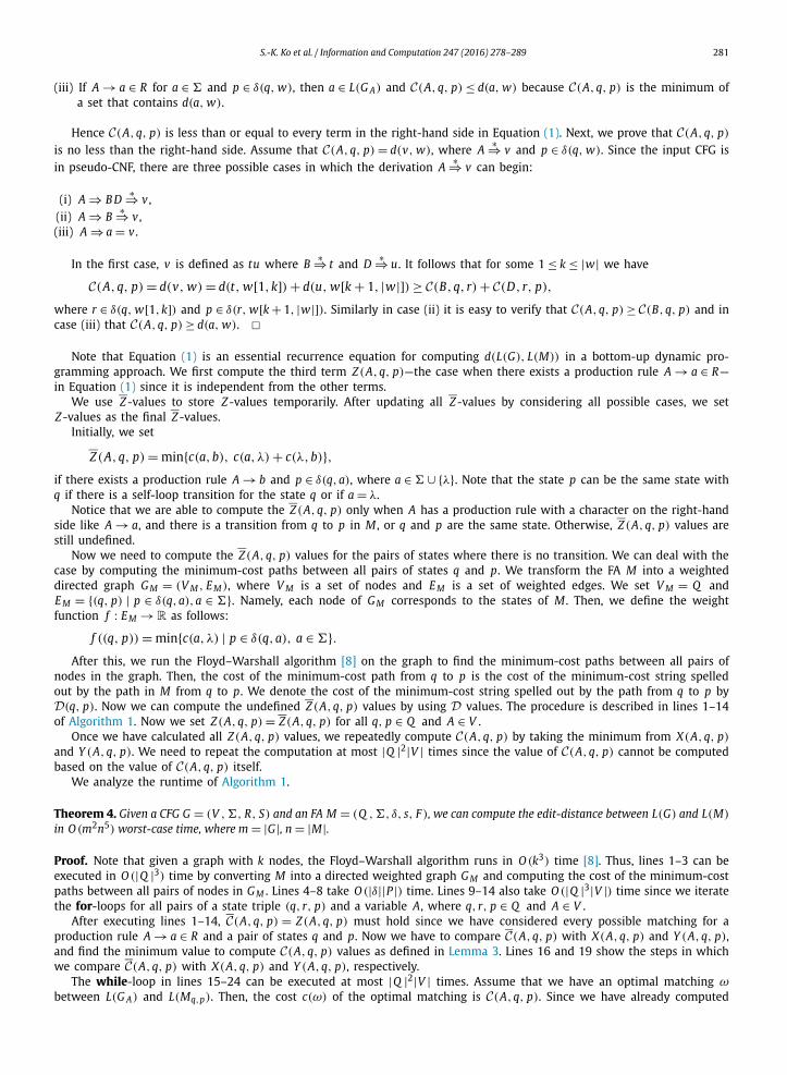
Algorithm 1 The algorithm for computing d(L(G), L(M)).Input: A CFG G = (V , �, R, S) and an FA M = (Q , �, δ, s, F )

1: for q, p ∈ Q do2: D(q, p) ← min{c(ω) | h(ω) = (w, λ), w ∈ L(Mq,p)}3: end for4: for p, q ∈ Q and A → b ∈ R do5: if p ∈ δ(q, a) then6: C(A, q, p) ← min{c(a, b), c(a, λ) + c(λ, b)}7: end if8: end for9: for q, r, p ∈ Q and A ∈ V do

10: C(A, q, p) ← min{C(A, q, p), D(q, r) + C(A, r, p)}11: end for12: for q, r, p ∈ Q and A ∈ V do13: C(A, q, p) ← min{C(A, q, p), C(A, q, r) +D(r, p)}14: end for15: while there is an updated C-value do16: for q, p ∈ Q do17: for A → B D ∈ R and r ∈ Q do18: C(A, q, p) ← min{C(A, q, p), C(B, q, r) + C(D, r, p)}19: end for20: for A → B ∈ R do21: C(A, q, p) ← min{C(A, q, p), C(B, q, p)}22: end for23: end for24: end while25: return min{C(S, s, f ) | f ∈ F }Output: d(L(G), L(M))

Z(A, q, p), now C(A, q, p) is the optimal matching between two strings, where a string from G is derived by one production rule of form A → a for A ∈ V and a ∈ �. Assume that we process the while-loop in lines 15–24 once and have an updated C(A, q, p)-value in line 18. After this C(A, q, p) is the cost of an optimal matching between a string derived by G A in two steps and a string of L(Mq,p). Note that C(A, q, p) can be updated based on the other C-values since we take the minimum between two values. This implies that the while-loop in lines 15–24 can be executed at most |Q |2|V | times because otherwise we always have to update C-value based on the same value.

The computation of lines 16–23 takes O (|Q |3|R|) time since we need to consider all production rules of G and all state triples of M in the double for-loops in lines 16 and 17. Therefore, the algorithm to compute the edit-distance between L(G)

and L(M) runs in time O (|Q |5|R||V |) and this value is upper bounded by O (m2n5). �Once we have calculated the edit-distance, we can also retrieve an optimal alignment by the traceback of the computa-

tion.

Theorem 5. Given a CFG G = (V , �, R, S) and an FA M = (Q , �, δ, s, F ), we can compute the optimal alignment between L(G) and L(M) in O (mnk) worst-case time, where m = |G|, n = |M| and k is the length of the optimal alignment.

Proof. We can retrieve the optimal alignment between a CFG G and an FA M that results in the edit-distance by the traceback. We can assume that all C-values are already computed during the computation of the edit-distance.

From C(S, s, f ), we trace back to the initial step to find the optimal alignment. For example, we check where the value of C(S, s, f ) is from by comparing C(S, s, f ) with the following cases:

(i) c(λ, b) if s = f and S → b ∈ R;(ii) c(a, b), c(a, λ) + c(λ, b) if there is a production rule S → b ∈ R and f ∈ δ(s, a);(iii) D(s, r1) + C(S, r1, r2) +D(r2, f );(iv) C(B, s, r) + C(D, r, f ) if there is a production rule S → B D ∈ R; and(v) C(A, s, f ) if there is a production rule S → A ∈ R .

By Algorithm 1, one of the five values should be equal to C(S, s, f ). Now assume that C(S, s, f ) = C(B, s, r) + C(D, r, f ). Then, we check where the values C(B, s, r) and C(D, r, f ) are from in a similar way. We repeat this procedure until we find matchings between all C-values and base cases (i)–(iii). After finding all matchings for all C-values, we can retrieve the corresponding alignment. Since we consider all production rules of G and states of M at each step of the traceback, it takes O (mnk) time to retrieve the optimal alignment, where k is the length of the optimal alignment. Note that k can be exponential in the size of G as the shortest string in L(G) can be of length 2|V |−1. If the FA M only accepts an empty string λ and the length of the shortest string accepted by G is 2|V |−1, then the length of the optimal alignment between L(G)

and L(M) should be exponential in the size of G . We present an asymptotic upper bound for the length k of an optimal alignment between L(G) and L(M) by analyzing Algorithm 1. After executing lines 1–12, we have optimal alignments

S.-K. Ko et al. / Information and Computation 247 (2016) 278–289 283

Fig. 1. Two examples of aligning x and y. The first alignment (a) has three short gaps and the second alignment (b) has one long gap.

of length O (|Q |) since we only consider the matchings between a string of length one derived by a production rule of form A → a ∈ R and a string from an FA M . Now we repeat the computations O (|Q |2|V |) times and each computation doubles the length of optimal alignments in the worst-case.

Therefore, the asymptotic upper bound for k is O (|Q | · 2|Q |2|V |) which is upper bounded by O (n · 2n2m).Finally, we mention that we can retrieve an optimal alignment in O (k) time if we save back-pointers when we run

Algorithm 1 since we do not need to scan all production rules of G and states of M at each step. �5. Affine gap distance

The approximate pattern matching problem is closely related to the sequence alignment problem in bioinformatics [19,20]. A biological sequence alignment is a process of arranging sequences of nucleotides describing DNA or RNA molecules, or protein amino acid sequences, and examining the similarity between the two sequences.

Consider the two alignments in Fig. 1. Both alignments have gaps—sequences of deletions, or sequences of insertions—of total length four. However, the second alignment is biologically better since the deletion of four consecutive elements is more likely to occur than the deletion or insertion of three separated elements. Therefore, it is desirable to assign a higher penalty to an alignment containing many short gaps than few long gaps. Assume that an alignment ω has k consecutive insertions or deletions—a gap of length k. Then, the cost of ω is linearly proportional to |ω|. Namely, c(ω) = g · |ω|, for a constant g . Instead of using this linear gap penalty function, we can use the affine gap penalty function that helps to obtain biologically better alignments [3,7].

Here the alphabet � of edit operations consists of deletions (a → λ), insertions (λ → a), substitutions (a → b) that change the symbol, and trivial substitutions (a → a) that do not change the symbol. We denote �del = {(a → λ) | a ∈ �}, �ins = {(λ → a) | a ∈ �}, �sub = {(a → b) | a, b ∈ �, a = b} and �triv = {(a → a) | a ∈ �}, and thus

� = �del ∪ �ins ∪ �sub ∪ �triv.

Let ω ∈ �+ be a sequence of edit operations. The (maximal) IDS-decomposition of ω (insertion–deletion–substitution de-composition of ω) is

compIDS(ω) = (ω1,ω2, . . . ,ωk),

where ω1ω2 . . .ωk = ω, ωi ∈ �+del ∪�+

ins ∪�+sub ∪�+

triv, for i = 1, . . . , k, and for any 1 ≤ j < k the strings ω j and ω j+1 belong to different sets �+

del, �+ins, �+

sub and �+triv, respectively.

Given ω, we can obtain the IDS-decomposition of ω by subdividing ω into maximal substrings each of which consists of only insertions, only deletions, only substitutions, or only trivial substitutions. Thus, compIDS(ω) is uniquely defined.

We define the affine gap cost of an IDS-decomposition as follows:

caffine(ω) =

⎧⎪⎨⎪⎩

l + g · |ω| if ω ∈ �+del ∪ �+

ins,

c(ω) if ω ∈ �+sub,

0 if ω ∈ �+triv,

where l and g are constants.We then define the affine gap cost of an arbitrary sequence of edit operations ω ∈ �+ , where compIDS(ω) =

(ω1, ω2, . . . , ωk), to be

caffine(ω) =k∑

i=1

caffine(ωi).

For a sequence of edit operations, the affine gap cost gives a constant l penalty for each gap opening (consisting of consecutive insertions or consecutive deletions) and an additional penalty that is linear in the length of the gap. We call the edit-distance based on the affine gap cost function the affine gap distance. We design an algorithm for computing the affine gap distance between a CFG and an FA. This is an extension of the previous algorithm, yet has the same time complexity. The main difference is that we define C-values with two additional parameters as follows:

284 S.-K. Ko et al. / Information and Computation 247 (2016) 278–289

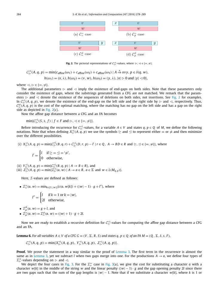
Fig. 2. The pictorial representations of C�

�-values, where �,� ∈ {=, =}.

C��(A,q, p) = min{caffine(ω1) + caffine(ω2) + caffine(ω3) | A∗⇒ xv y, p ∈ δ(q, w),

h(ω1) = (x, λ),h(ω2) = (v, w),h(ω3) = (y, λ), |x| � 0 and |y| � 0},where �, � ∈ {=, =}.

The additional parameters � and � imply the existence of end-gaps on both sides. Note that these parameters only consider the existence of gaps, where the substrings generated from a CFG are not matched. We remark that the param-eters � and � denote the existence of the sequences of deletions on both sides, not insertions. See Fig. 2 for examples. In C�� (A, q, p), we denote the existence of the end-gap on the left side and the right side by � and �, respectively. Thus, C == (A, q, p) is the cost of the optimal matching, where the matching has no gap on the left side and has a gap on the right side as depicted in Fig. 2(c).

Now the affine gap distance between a CFG and an FA becomes

min{C��(S, s, f ) | f ∈ F and �,� ∈ {=, =}}.Before introducing the recurrence for C�� -values, for a variable A ∈ V and states q, p ∈ Q of M , we define the following

notations. Note that when defining X��(A, q, p) we use the symbols � and � to represent either = or = and then minimize over the different possibilities.

(i) X��(A, q, p) = min{C�� (B, q, r) + C�� (D, r, p) − l′ | r ∈ Q , A → B D ∈ R and �, � ∈ {=, =}}, where

l′ ={

l if � = � = ‘=’,

0 otherwise,

(ii) Y �� (A, q, p) = min{C�� (B, q, p) | A → B ∈ R}, and(iii) Z��(A, q, p) = min{I�� (a, w) | A → a ∈ R, a ∈ � and w ∈ L(Mq,p)}.

Here, I-values are defined as follows:

• I== (a, w) = mink∈[1,|w|]{c(a, w[k]) + (|w| − 1) · g + l′′}, where

l′′ ={

l if k = 1 or k = |w|,2l otherwise,

• I == (a, w) = g + l, and

• I== (a, w) = I == (a, w) = (|w| + 1) · g + 2l.

Now we are ready to establish a recursive definition for C�� -values for computing the affine gap distance between a CFG and an FA.

Lemma 6. For all variables A ∈ V of a CFG G = (V , �, R, S) and states q, p ∈ Q of an FA M = (Q , �, δ, s, F ),

C��(A,q, p) = min{X��(A,q, p), Y �� (A,q, p), Z��(A,q, p)}.

Proof. We prove the statement in a way similar to the proof of Lemma 3. The first term in the recurrence is almost the same as in Lemma 3, yet we subtract l when two gaps merge into one. For the productions A → a, we define four types of I�� -values depending on � and �.

We depict the four cases in Fig. 3. For the I== case in Fig. 3(a), we give the cost for substituting a character a with a character w[k] in the middle of the string w and the linear penalty (|w| − 1) · g and the gap opening penalty 2l since there are two gaps such that the sum of the gap lengths is |w| − 1. Note that if we substitute a character w[k], where k is 1 or

S.-K. Ko et al. / Information and Computation 247 (2016) 278–289 285

Fig. 3. The pictorial representations of I�

�-values where �,� ∈ {=, =}.

|w|, then the gap opening penalty should be l since there is only one gap. Now we consider the I== and I == cases depicted in Fig. 3(b) and Fig. 3(c). Since there are two gaps of total length |w| + 1, we assign the linear penalty (|w| + 1) · g and the gap opening penalty 2l. Lastly, Fig. 3(d) represents the I =

= case. Since there is only one gap of length 1, the cost becomes g + l. After these observations the remaining proof is similar to the proof for Lemma 3. �

Note that the time complexity of this algorithm remains essentially the same as the time used by Algorithm 1. Since we consider the four variations of C-values, the time complexity only increases to four times the runtime of Algorithm 1.

Theorem 7. Given a CFG G and an FA M, we can compute the affine gap distance between L(G) and L(M) in O (m2n5) worst-case time, where m = |G| and n = |M|.

Theorem 8. Given a CFG G and an FA M, we can compute the optimal alignment for the affine gap distance between L(G) and L(M)

in O (mnk) worst-case time, where m = |G|, n = |M| and k is the length of the optimal alignment.

6. Concave gap distance

Several researchers considered non-linear gap penalty functions, including the affine gap penalty function [3,7,12,16,23]. Although the affine gap penalty function prefers few longer gaps to many smaller gaps, we cannot guarantee that the affine gap penalty function always produces the best result. For example, assume that there are two alignments s1 and s2 for two sequences—s1 contains two gaps of length 99 and 100, and s2 contains just one gap of length 240. Let us assume that the remaining parts of s1 and s2 are perfectly matched without any substitutions. By employing the affine gap penalty function with l = 5 and g = 1, we obtain c(s1) = 99 + 100 + 5 × 2 = 209 and c(s2) = 240 + 5 = 245. Even though the gap opening penalty is considered in the affine gap distance, it may not be optimal for some practical cases such as this example. This is why the concave gap distance is introduced [12,16,23].

Now we define the concave gap cost of ω as follows:

cconcave(ω) =

⎧⎪⎨⎪⎩

l + g · log |ω| if ω ∈ �+del ∪ �+

ins,

c(ω) if ω ∈ �+sub,

0 if ω ∈ �+triv,

where l and g are constants.The concave gap cost of an arbitrary sequence of edit operations ω ∈ �+ , where compIDS(ω) = (ω1, ω2, . . . , ωk) is then

cconcave(ω) =k∑

i=1

cconcave(ωi).

Under this gap penalty function, the shape of the penalty score with respect to the length of the gap is concave in the sense that its forward differences are non-increasing. Fig. 4 illustrates the difference among the three gap penalty functions: linear, affine and concave gap penalty functions.

We define new C-values for computing the concave gap distance as follows:

C ji (A,q, p) = min{cconcave(ω1) + cconcave(ω2) + cconcave(ω3) | A

∗⇒ xv y,

p ∈ δ(q, w),h(ω ) = (x, λ),h(ω ) = (v, w),h(ω ) = (y, λ), |x| = i and |y| = j}.

1 2 3

286 S.-K. Ko et al. / Information and Computation 247 (2016) 278–289

Fig. 4. Comparison of the linear, affine and concave gap costs for a sequence of deletions or insertions ω.

Fig. 5. The pictorial representations of C-values where i, j ∈N.

We use two additional parameters for maintaining the lengths of gaps on both sides. In C ji (A, q, p), i and j mean the

length of the end-gap on the left side and the length of the end-gap on the right side, respectively. We depict the pictorial representations of the four cases in Fig. 5.

We let V(t) be the set of variables that can derive terminal strings of length t:

V(t) = {A | A ∈ V , w ∈ L(G A) and |w| = t}.We can compute V(t) as follows:

t−1⋃k=1

{A | A → B D ∈ R, (B, D) ∈ V(k) × V(t − k)}

∪ {A | A → B ∈ R, B ∈ V(t)} ∪ Zt,

where

Zt ={

{A | A → a ∈ R} if t = 1,

∅ if t = 1.

Next, before introducing the recurrence for C-values for the concave gap distance, we define the following values corre-sponding to a variable A ∈ V and states q, p ∈ Q of M:

(i) X ji (A, q, p) = min{Cm

i (B, q, r) + C jn(D, r, p) + l1 | r ∈ Q , A → B D ∈ R}, where

l1 ={

g · log |m+nmn | − l if mn = 0,

0 otherwise,

(ii) Y ji (A, q, p) = min{C j−t

i (B, q, p) + l2 | A → B D ∈ R, t ∈ [1, j], D ∈ V(t)}, where

l2 ={

l + g · log j if j = t,

g · log jj−t otherwise,

(iii) Z j(A, q, p) = min{C j

(D, q, p) + l3 | A → B D ∈ R, t ∈ [1, i], B ∈ V(t)}, where

i i−t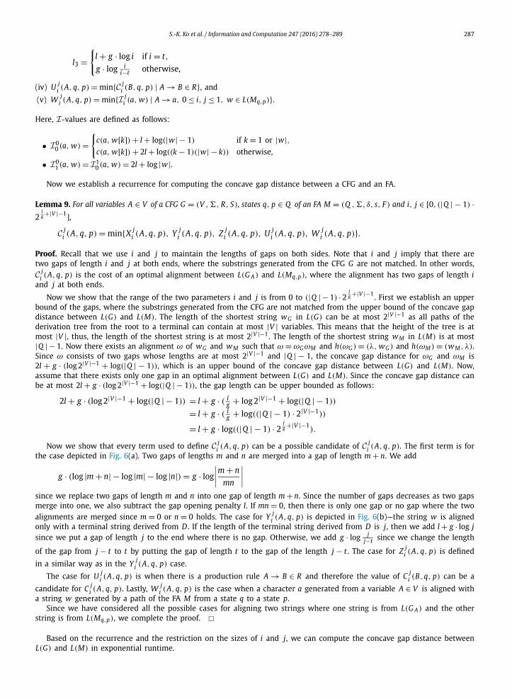

S.-K. Ko et al. / Information and Computation 247 (2016) 278–289 287

l3 ={

l + g · log i if i = t,

g · log ii−t otherwise,

(iv) U ji (A, q, p) = min{C j

i (B, q, p) | A → B ∈ R}, and

(v) W ji (A, q, p) = min{I j

i (a, w) | A → a, 0 ≤ i, j ≤ 1, w ∈ L(Mq,p)}.

Here, I-values are defined as follows:

• I00 (a, w) =

{c(a, w[k]) + l + log(|w| − 1) if k = 1 or |w|,c(a, w[k]) + 2l + log((k − 1)(|w| − k)) otherwise,

• I01 (a, w) = I1

0 (a, w) = 2l + log |w|.

Now we establish a recurrence for computing the concave gap distance between a CFG and an FA.

Lemma 9. For all variables A ∈ V of a CFG G = (V , �, R, S), states q, p ∈ Q of an FA M = (Q , �, δ, s, F ) and i, j ∈ [0, (|Q | − 1) ·2

lg +|V |−1],

C ji (A,q, p) = min{X j

i (A,q, p), Y ji (A,q, p), Z j

i (A,q, p), U ji (A,q, p), W j

i (A,q, p)}.Proof. Recall that we use i and j to maintain the lengths of gaps on both sides. Note that i and j imply that there are two gaps of length i and j at both ends, where the substrings generated from the CFG G are not matched. In other words, C j

i (A, q, p) is the cost of an optimal alignment between L(G A) and L(Mq,p), where the alignment has two gaps of length iand j at both ends.

Now we show that the range of the two parameters i and j is from 0 to (|Q | − 1) · 2lg +|V |−1. First we establish an upper

bound of the gaps, where the substrings generated from the CFG are not matched from the upper bound of the concave gap distance between L(G) and L(M). The length of the shortest string wG in L(G) can be at most 2|V |−1 as all paths of the derivation tree from the root to a terminal can contain at most |V | variables. This means that the height of the tree is at most |V |, thus, the length of the shortest string is at most 2|V |−1. The length of the shortest string w M in L(M) is at most |Q | − 1. Now there exists an alignment ω of wG and w M such that ω = ωGωM and h(ωG) = (λ, wG) and h(ωM) = (w M , λ). Since ω consists of two gaps whose lengths are at most 2|V |−1 and |Q | − 1, the concave gap distance for ωG and ωM is 2l + g · (log 2|V |−1 + log(|Q | − 1)), which is an upper bound of the concave gap distance between L(G) and L(M). Now, assume that there exists only one gap in an optimal alignment between L(G) and L(M). Since the concave gap distance can be at most 2l + g · (log 2|V |−1 + log(|Q | − 1)), the gap length can be upper bounded as follows:

2l + g · (log 2|V |−1 + log(|Q | − 1)) = l + g · ( lg + log 2|V |−1 + log(|Q | − 1))

= l + g · ( lg + log((|Q | − 1) · 2|V |−1))

= l + g · log((|Q | − 1) · 2lg +|V |−1

).

Now we show that every term used to define C ji (A, q, p) can be a possible candidate of C j

i (A, q, p). The first term is for the case depicted in Fig. 6(a). Two gaps of lengths m and n are merged into a gap of length m + n. We add

g · (log |m + n| − log |m| − log |n|) = g · log

∣∣∣∣m + n

mn

∣∣∣∣since we replace two gaps of length m and n into one gap of length m + n. Since the number of gaps decreases as two gaps merge into one, we also subtract the gap opening penalty l. If mn = 0, then there is only one gap or no gap where the two alignments are merged since m = 0 or n = 0 holds. The case for Y j

i (A, q, p) is depicted in Fig. 6(b)—the string w is aligned only with a terminal string derived from D . If the length of the terminal string derived from D is j, then we add l + g · log jsince we put a gap of length j to the end where there is no gap. Otherwise, we add g · log j

j−t since we change the length

of the gap from j − t to t by putting the gap of length t to the gap of the length j − t . The case for Z ji (A, q, p) is defined

in a similar way as in the Y ji (A, q, p) case.

The case for U ji (A, q, p) is when there is a production rule A → B ∈ R and therefore the value of C j

i (B, q, p) can be a candidate for C j

i (A, q, p). Lastly, W ji (A, q, p) is the case when a character a generated from a variable A ∈ V is aligned with

a string w generated by a path of the FA M from a state q to a state p.Since we have considered all the possible cases for aligning two strings where one string is from L(G A) and the other

string is from L(Mq,p), we complete the proof. �Based on the recurrence and the restriction on the sizes of i and j, we can compute the concave gap distance between

L(G) and L(M) in exponential runtime.

288 S.-K. Ko et al. / Information and Computation 247 (2016) 278–289

Fig. 6. The pictorial representations of three cases in the recursive definition of C-values.

Theorem 10. Given a CFG G = (V , �, R, S) and an FA M = (Q , �, δ, s, F ), we can compute the concave gap distance between L(G)

and L(M) in O (m5n88m log3 n) worst-case time, where m = |G| and n = |M|.

Proof. We can compute the concave gap distance between L(G) and L(M) by computing C-values defined in Lemma 9. Among all C-values, the minimum of C j

i (S, s, f ), where f ∈ F and i, j ∈ [0, (|Q | − 1) · 2lg +|V |−1], is the concave gap distance

between L(G) and L(M). We need to compute all C-values in the worst-case. Since the upper bound of the concave gap distance is 2l + g · (log 2|V |−1 + log(|Q | − 1)), the multiplication of the lengths of two end-gaps should be at most 2|V |−1 ·(|Q | − 1). Therefore, the number of the lengths of two end-gaps to be computed is

2|V |−1·(|Q |−1)∑i=1

2|V |−1 · (|Q | − 1)

i.

Since

k∑i=1

k

i∈ O (k log k),

the upper bound of the number of entries to be computed is

O (|V ||Q |2 · |Q ||V | · 2|V | · log |Q |) = O (|V |2|Q |3 · 2|V | · log |Q |)if we assume g and l as constants.

First, we need

O (|Q |5|R||V |2 · 4|V | · log2 |Q |)time to compute all C-values once. Note that the computed C(A, q, p)-value is not necessarily correct since the value can be updated as we iterate the process. Note that the number of iterations required to compute correct C-values is equivalent to the number of entries to be computed. This implies that we need to iterate O (|V |2|Q |3 · 2|V | · log |Q |) times. Now the worst-case time complexity for computing the concave gap distance between L(G) and L(M) is O (|V |4|R||Q |8 ·8|V | · log3 |Q |)which is upper bounded by O (m5n88m log3 n), where m is the size of the CFG G and n is the size of the FA M . �7. Conclusions

We have considered the problem of approximately matching a context-free language and a regular language. We have examined three types of gap cost functions that are used for approximate string matching: linear, affine and concave. Based on the dynamic programming approach, we have introduced algorithms for computing the linear, affine and concave gap distance between a CFG and an FA.

Given a CFG of size m and an FA of size n, we have presented algorithms for computing linear and affine gap distances in O (m2n5) time. We have also shown that computing the optimal alignment of length k takes O (mnk) time by our algo-rithm when we consider linear or affine gap distance. Finally, we have proposed an O (m5n88m log3 n) time algorithm for computing the concave gap distance.

It will be interesting to see if we can compute the max–min distance between a CFG and an FA, or find k optimal alignments between a CFG and an FA.

S.-K. Ko et al. / Information and Computation 247 (2016) 278–289 289

Acknowledgments

We thank the anonymous referees for a careful reading of an earlier version of the paper and for many useful suggestions that have improved the presentation.

Ko and Han were supported by the Basic Science Research Program through NRF funded by MEST (2015R1D1A1A01060097), the Yonsei University Future-leading Research Initiative of 2015 and the International Cooperation Program managed by NRF of Korea (2014K2A1A2048512), and Salomaa was supported by the Natural Sciences and Engineering Research Council of Canada Grant OGP0147224.

References

[1] A. Aho, T. Peterson, A minimum distance error-correcting parser for context-free languages, SIAM J. Comput. 1 (4) (1972) 305–312.[2] Y. Bar-Hillel, M. Perles, E. Shamir, On formal properties of simple phrase structure grammars, in: Y. Bar-Hillel (Ed.), Language and Information: Selected

Essays on Their Theory and Application, Addison–Wesley, Reading, Massachusetts, 1964, pp. 116–150, chapter 9.[3] G.J. Barton, M.J.E. Sternberg, Evaluation and improvements in the automatic alignment of protein sequences, Protein Eng. 1 (2) (1987) 89–94.[4] E. Brill, R.C. Moore, An improved error model for noisy channel spelling correction, in: Proceedings of the 38th Annual Meeting on Association for

Computational Linguistics, 2000, pp. 286–293.[5] C. Choffrut, G. Pighizzini, Distances between languages and reflexivity of relations, Theor. Comput. Sci. 286 (1) (2002) 117–138.[6] J. Earley, An efficient context-free parsing algorithm, Commun. ACM 13 (2) (1970) 94–102.[7] W.M. Fitch, T.F. Smith, Optimal sequence alignments, in: Proceedings of the National Academy of Sciences, vol. 80, 1983, pp. 1382–1386.[8] R.W. Floyd, Algorithm 97: shortest path, Commun. ACM 5 (6) (1962) 345–348.[9] Y.-S. Han, S.-K. Ko, K. Salomaa, The edit-distance between a regular language and a context-free language, Int. J. Found. Comput. Sci. 24 (7) (2013)

1067–1082.[10] J. Hopcroft, J. Ullman, Introduction to Automata Theory, Languages, and Computation, 2nd ed., Addison–Wesley, Reading, MA, 1979.[11] L. Kari, S. Konstantinidis, Descriptional complexity of error/edit systems, J. Autom. Lang. Comb. 9 (2004) 293–309.[12] J.R. Knight, E.W. Myers, Approximate regular expression pattern matching with concave gap penalties, Algorithmica 14 (1995) 67–78.[13] S. Konstantinidis, Computing the edit distance of a regular language, Inf. Comput. 205 (2007) 1307–1316.[14] V.I. Levenshtein, Binary codes capable of correcting deletions, insertions, and reversals, Sov. Phys. Dokl. 10 (8) (1966) 707–710.[15] G. Lyon, Syntax-directed least-errors analysis for context-free languages: a practical approach, Commun. ACM 17 (1) (1974) 3–14.[16] W. Miller, E.W. Myers, Sequence comparison with concave weighting functions, Bull. Math. Biol. 50 (2) (1988) 97–120.[17] M. Mohri, Edit-distance of weighted automata: general definitions and algorithms, Int. J. Found. Comput. Sci. 14 (6) (2003) 957–982.[18] G. Myers, Approximately matching context-free languages, Inf. Process. Lett. 54 (1995) 85–92.[19] S.B. Needleman, C.D. Wunsch, A general method applicable to the search for similarities in the amino acid sequence of two proteins, J. Mol. Biol. 48 (3)

(1970) 443–453.[20] D. Sankoff, J.B. Kruskal, Time Warps, String Edits, and Macromolecules: The Theory and Practice of Sequence Comparison, Addison–Wesley, 1983.[21] S. Sippu, E. Soisalon-Soininen, Parsing Theory: Languages and Parsing, EATCS Monographs on Theoretical Computer Science, vol. 1, Springer-Verlag,

1988.[22] W.F. Tichy, The string-to-string correction problem with block moves, ACM Trans. Comput. Syst. 2 (4) (1984) 309–321.[23] M.S. Waterman, Efficient sequence alignment algorithms, J. Theor. Biol. 108 (1984) 333–337.[24] D. Wood, Theory of Computation, Harper & Row, 1987.