Influence of dynamic soil-structure interaction analyses ...
204
Influence of dynamic soil-structure interaction analyses on shear buildings Dissertation submitted to and approved by the Department of Architecture, Civil Engineering and Environmental Sciences University of Braunschweig – Institute of Technology and the Faculty of Engineering University of Florence in candidacy for the degree of a Doktor-Ingenieur (Dr.-Ing.) / Dottore di Ricerca in Mitigation of risk due to natural hazards on structures and infrastructures *) by Stefano Renzi 28.08.1975 from Prato, Italy Submitted on 23 September 2009 Oral examination on 06 November 2009 Professorial advisors Prof. Joachim Stahlmann Prof. Giovanni Vannucchi 2009 *) Either the German or the Italian form of the title may be used.
Transcript of Influence of dynamic soil-structure interaction analyses ...
Influence of dynamic soil-structure interaction analyses
on shear buildings
Dissertation
submitted to and approved by the
Department of Architecture, Civil Engineering and Environmental Sciences
University of Braunschweig – Institute of Technology
and the
Faculty of Engineering
University of Florence
in candidacy for the degree of a
Doktor-Ingenieur (Dr.-Ing.) /
Dottore di Ricerca in Mitigation of risk due to natural hazards
on structures and infrastructures*)
by
Stefano Renzi
28.08.1975
from Prato, Italy
Submitted on 23 September 2009
Oral examination on 06 November 2009
Professorial advisors Prof. Joachim Stahlmann
Prof. Giovanni Vannucchi
2009
*) Either the German or the Italian form of the title may be used.

The dissertation is published in an electronic form by the Braunschweig University
library at the address
http://www.biblio.tu-bs.de/ediss/data/

Tutors Prof. Dr.-Ing. Giovanni Vannucchi University of Florence Prof. Dr.-Ing. Joachim Stahlmann Technical University of Braunschweig Prof. Dr.-Ing. George Mylonakis University of Patras Prof. Dr.-Ing. Claudia Madiai University of Florence Doctoral course coordinators Prof. Dr.-Ing. Claudio Borri University of Florence Prof. Dr.-Ing. Udo Peil Technical University of Braunschweig
Examining Committee Prof. Dr.-Ing. Giovanni Vannucchi University of Florence Prof. Dr.-Ing. Joachim Stahlmann Technical University of Braunschweig Prof. Dr.-Ing. Claudia Madiai University of Florence Prof. Dr.-Ing. Udo Peil Technical University of Braunschweig Prof. Dr.-Ing. Marcello Ciampoli University of Rome “La Sapienza” Prof. Dr.-Ing. Luz Lehman Technical University of Braunschweig Prof. Dr.-Ing. Vincenzo Sepe University of Chieti-Pescara Prof. Dr.-Ing. Dieter Dinkler Technical University of Braunschweig


To Carlotta, the milestone of my life
she always supported and encouraged me
To Laura and Lorenzo
my precious jewels

v i i
Abstract
Risk management is a modern concept concerning the way to cope with natural and man-
induced catastrophic events. Definitions of risk are reported and discussed with particular relevance
on seismic risk for the built environment. Due to evidences of historical earthquakes, the importance
of achieving an acceptable level of safety for ordinary reinforced-concrete structures, as “element at
risk”, is undisputed. It is also well known that Soil-Structure Interaction (SSI) can give a relevant
contribution to the correct evaluation of the phenomena, even if the topic is not free of
misconceptions. Despite extensive research over than 30 years in this subject, there is still
controversy regarding the role of SSI in the seismic performance of structures founded on soft soil.
Neglecting SSI effects is currently being suggested in many seismic codes (ATC-3, NEHRP-97) as
a conservative simplification that would supposedly lead to improved safety margins.
It should be emphasized that the interest in studying the seismic SSI is motivated by the
necessity of computing the effective earthquake excitation to a structure (which is also called
Foundation Input Motion, or FIM) with respect to the free-field ground motion. The latter strongly
influences the structure seismic demand as it takes into account both the soil-foundation coupling
(i.e. the dynamic impedance function of the soil-foundation system) and the scattering effects
caused by the motion of foundations (i.e. the kinematic interaction effects). It is rather unfortunate
that kinematic interaction effects are often neglected in engineering practice due to the difficulties
of their evaluation even though they may be relevant.
In general, a rigorous assessment of seismic SSI is not a simple task because of the difficulties
associated with the evaluation of kinematic interaction and scattering effects. Therefore a solution
to this problem that is capable of offering a satisfactory trade-off between rigor and simplicity is
highly desirable especially in standard engineering practice.
This doctoral work focuses on the hazard and structural vulnerability assessment of ordinary
reinforced-concrete structures with respect to seismic risk and attempts to make two main
contributions with regards to structures founded on superficial foundation.
First, a systematic application of complete SSI analyses to different types of buildings (up to
twenty storeys), has been performed; the compliance of the ground has been evaluated by means of
the computer program SASSI2000 (Lysmer et al., 1999). Concrete shear-type structures have been
modeled as generalized Single Degree Of Freedom (SDOF) systems using the principle of virtual
displacements, while different soil conditions (consistent with the EC8-I), foundation depths and
seismic excitations are taken into account. The modified characteristics of the buildings, in terms of
modified damping and period, have been estimated, comparing a classical solution (Wolf, 1985) and
a recent exact procedure (Mylonakis, 2006); results are presented in form of ready-to-use non-
dimensional charts.
The second main contribution of this work is a sort of “pre-normative" study concerning SSI
assessment, which could be useful to enhance the codes, as a measure of risk mitigation; SSI effect
has been evaluated in terms of maximum displacements/accelerations at the top of the buildings and
a systematic comparison with the fixed-base solutions has been performed. The final goal is the set-
up of simplified charts and tables that can be easily used by practitioners who want to face the task
of SSI in an immediate and simplified manner, without performing an expensive and time-
consuming, albeit absolutely necessary over all the design steps for important and strategic
structures (such as bridge piers or power plants) analysis.

v i i i
Such tool could be very useful for engineers, especially concerning the design of medium-rise
reinforced-concrete buildings and/or for pre-design stages, where the SSI effect must be estimated
and cannot be excluded a priori.
The previously mentioned simplified dimensionless charts make possible an attempt of
generalization. Although this is only a first step towards this ambitious goal, it shows all the
difficulties which have to be overcome but also highlights some interesting and promising results.


x
Acknowledgment
Without the precious help of my collaborators and tutors I would have not achieved my goal
of studying this complex topic and completing the work on my PhD thesis.
Thanks go in particular to Prof. Mylonakis who gave me hospitality in Patras and made me
feel like at home; he guided me in this topic and inspired me the profound interest in going always
deeper in the research.
Thanks also to my tutors, Prof. Giovanni Vannucchi, Prof. Joachim Stahlmann and Prof.
Claudia Madia for the guidance, and collaboration.
I would finally thank all the people from all around the world I have met during this hard
work; all of them gave directly or indirectly a contribution to the proceeding of the thesis.

x i i
Contents
Chapter 1 Risk and Hazard in Civil Engineering ................................................................. 1
1.1 Introduction ................................................................................................................ 1
1.2 Risk Management Framework ................................................................................... 2
1.2.1 Risk assessment ...................................................................................................... 2
1.2.2 Risk treatment ......................................................................................................... 5
1.3 Earthquake Risk and Hazard ...................................................................................... 7
1.4 Contribution of the present research work ............................................................... 10
Chapter 2 Dynamic Soil-Structure Interaction (SSI) .......................................................... 12
2.1 Introduction .............................................................................................................. 12
2.2 Complex stiffness matrix.......................................................................................... 13
2.3 Current methodology to SSI analyses ...................................................................... 14
2.4 Kinematic and Inertial Interaction ............................................................................ 18
2.4.1 Assessing the effects of Kinematic Interaction .................................................... 18
2.4.2 Inertial SSI: assessment of foundation “springs” and “dashpots” ........................ 20
2.4.3 Computing dynamic impedances .......................................................................... 25
2.5 Effect of SSI ............................................................................................................. 27
2.5.1 Solution by Veletsos and co-workers (1974, 1975, 1977).................................... 29
2.5.2 Solution by Wolf (1985) ....................................................................................... 30
2.5.3 Solution by Mylonakis (2007) .............................................................................. 30
2.6 Dimensionless parameter ......................................................................................... 32
2.7 SSI – Beneficial or detrimental? .............................................................................. 34
2.7.1 SSI and seismic code spectra ................................................................................ 34
2.7.2 Ductility in Flexibly-Supported Structures ........................................................... 39
x i i i
Chapter 3 The computer program SASSI2000 .................................................................... 43
3.1 Introduction .............................................................................................................. 43
3.2 Substructuring methods in SASSI2000 analysis ....................................................... 44
3.2.1 The Flexible Volume Method (FVM) .................................................................. 44
3.2.2 The Substructure Subtraction Method (SM) ......................................................... 48
3.3 Computational steps ................................................................................................. 48
3.4 Site response analysis ............................................................................................... 50
3.4.1 Eigenvalue problem for generalized Rayleigh wave motion ................................ 51
3.4.2 Eigenvalue problem for generalized Love wave motion ...................................... 53
3.5 Transmitting boundary matrices ............................................................................... 54
3.6 Free-field motion ...................................................................................................... 54
3.7 Modeling of semi-infinite halfspace at base............................................................. 56
3.8 Impedance analysis ................................................................................................... 57
3.9 Computer program organization .............................................................................. 59
3.10 Capabilities and limitations ...................................................................................... 60
Chapter 4 Generalized Single Degree of Freedom Systems ............................................... 62
4.1 Introduction .............................................................................................................. 62
4.2 Lumped-mass system: shear building ...................................................................... 63
4.3 Assumed shape vector .............................................................................................. 63
4.4 Equation of motion ................................................................................................... 64
4.5 Response analysis ..................................................................................................... 65
4.6 Peak earthquake response ......................................................................................... 65
4.7 Selection of the shape function ................................................................................ 67
4.8 Generalized properties for an SSI system ................................................................ 68
4.9 Generalized SDOF of a floor slab ............................................................................ 70
Chapter 5 Performed analyses and results........................................................................... 72
5.1 Introduction .............................................................................................................. 72
5.2 Seismic Inputs .......................................................................................................... 73
5.2.1 Spectrum-matching earthquakes ........................................................................... 74
5.2.2 Near-Fault registered earthquakes ........................................................................ 75
5.3 Soil configurations ................................................................................................... 77

x i v
5.4 Selected Shear-Buildings ......................................................................................... 78
5.5 Foundation vibration analyses .................................................................................. 81
5.5.1 Modified damping and period .............................................................................. 84
5.5.2 Simplified dimensionless charts ........................................................................... 86
5.6 Seismic SSI analyses .............................................................................................. 124
5.6.1 Results from EC8-I design spectra ..................................................................... 125
5.6.2 Results from actual Near-Fault earthquakes ....................................................... 144
5.7 Considerations on the performed analysis .............................................................. 151
General conclusions and outlook......................................................................................... 153
Appendix A: Impedance Matrices ...................................................................................... 154
Appendix B Selected Earthquakes ...................................................................................... 182
References.............................................................................................................................. 185

Chapter 1 Risk and Hazard in Civil Engineering
1
Chapter 1
Risk and Hazard in Civil Engineering
1.1 Introduction
Risk Management is a process gaining more importance and increasing attention in Civil
Engineering in the last years. Diverse tasks were historically included in the definition of risk
management.
Around the late 1990´s the focus on possible losses and acceptable risk criteria on the basis of
risk-based and not only reliability based approach has received significantly more attention and
several research groups have been raised. Due-to the large variety of topics to which the task of risk
management was applied some confusion resulted, because several definitions for similar principles
exist. The definition of risk serves well as example. While in colloquial use the word risk is
sometimes applied for the hazard itself, other definitions are frequently found within recent
publications:
Risk = Probability x Damage
Risk = Probability x Consequences
Risk = Hazard x Vulnerability x Exposure
All have in common the combination of the probability or frequency of an event and its
implication on the considered system. Now, although this adaptability of the definition is certainly a
key strength it creates confusion. Regarding the outcome of risk based calculations the units
describing the risk have to be the same, no matter what definition is utilized. Thus, it is crucial not
to concentrate on the definitions themselves at first, but on the process to realize the connection of
the different parts. In this way it will not only be possible to clarify misunderstandings related to
different definitions, but furthermore an integrated approach will be achieved, which is applicable
in every discipline. After this is done, the definitions for major parts of the overall risk management
process will be derived and used further in this study (1).
Chapter 1 Risk and Hazard in Civil Engineering
2
1.2 Risk Management Framework
The analysis and management of natural disaster risk is a high multidisciplinary field of
research. It involves the work of natural scientists to determine the hazard characteristic parameters
such as probability of occurrence and intensity of an event for a special location, followed by a
profound engineering analysis about the building structure and infrastructural responses due to
natural disaster loads. Moreover, investigations of economists are needed to estimate the monetary
consequences of the damages and harms to the affected region, resulting in a political discussion
about how to handle the peril in order to guarantee an adequate safety level for society (2).
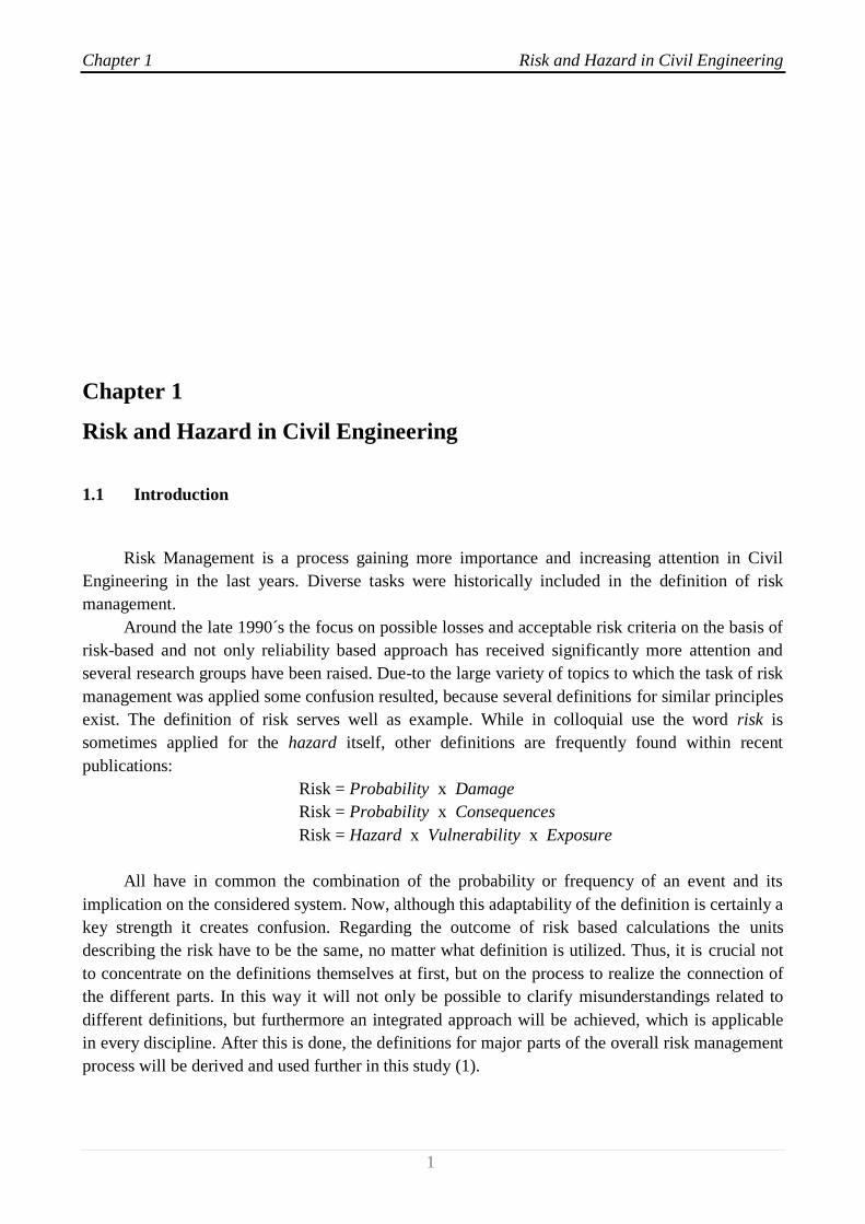
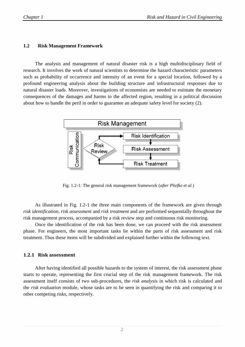
Fig. 1.2-1: The general risk management framework (after Pliefke et al.)
As illustrated in Fig. 1.2-1 the three main components of the framework are given through
risk identification, risk assessment and risk treatment and are performed sequentially throughout the
risk management process, accompanied by a risk review step and continuous risk monitoring.
Once the identification of the risk has been done, we can proceed with the risk assessment
phase. For engineers, the most important tasks lie within the parts of risk assessment and risk
treatment. Thus these items will be subdivided and explained further within the following text.
1.2.1 Risk assessment
After having identified all possible hazards to the system of interest, the risk assessment phase
starts to operate, representing the first crucial step of the risk management framework. The risk
assessment itself consists of two sub-procedures, the risk analysis in which risk is calculated and
the risk evaluation module, whose tasks are to be seen in quantifying the risk and comparing it to
other competing risks, respectively.
Chapter 1 Risk and Hazard in Civil Engineering
3
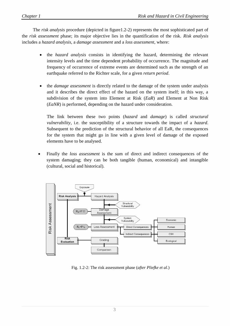
The risk analysis procedure (depicted in figure1.2-2) represents the most sophisticated part of
the risk assessment phase; its major objective lies in the quantification of the risk. Risk analysis
includes a hazard analysis, a damage assessment and a loss assessment, where:
the hazard analysis consists in identifying the hazard, determining the relevant
intensity levels and the time dependent probability of occurrence. The magnitude and
frequency of occurrence of extreme events are determined such as the strength of an
earthquake referred to the Richter scale, for a given return period.
the damage assessment is directly related to the damage of the system under analysis
and it describes the direct effect of the hazard on the system itself; in this way, a
subdivision of the system into Element at Risk (EaR) and Element at Non Risk
(EaNR) is performed, depending on the hazard under consideration.
The link between these two points (hazard and damage) is called structural
vulnerability, i.e. the susceptibility of a structure towards the impact of a hazard.
Subsequent to the prediction of the structural behavior of all EaR, the consequences
for the system that might go in line with a given level of damage of the exposed
elements have to be analysed.
Finally the loss assessment is the sum of direct and indirect consequences of the
system damaging; they can be both tangible (human, economical) and intangible
(cultural, social and historical).
Fig. 1.2-2: The risk assessment phase (after Pliefke et al.)
Chapter 1 Risk and Hazard in Civil Engineering
4
The risk analysis phase terminates with the quantification of risk where all the previously
collected information is comprised. It is distinguished between two different types of risk.
Firstly, risk can be calculated by taking the product of the annual probability of occurrence of
the hazard multiplied by the expected damage that goes in line with it.
Structural Risk = Probability x Damage [Damage measure / year]
It is being referred to as structural risk. Evidently, the structural risk is of primary importance
for engineers in order to predict the behavior and the response of a structure or structural element
under potential hazard load.
The second way to express the risk is to take the product of the annual probability of
occurrence of the hazard and the expected loss.
Total Risk = Probability x Loss [Loss unit / year]
It is being referred to as total risk. The total risk may comprise all consequences, both
tangible and intangible, if a reasonable way has been found to convert the primarily non appraisable
harms into monetary units. Alternatively, this transformation of intangible outcomes does not need
to be done and the total risk can be split according to the respective consequence classes to indicate
their relative contribution to risk. In any case the total risk is more exhaustive than the structural
risk as the full hazard potential to the system is taken in account (2).
The risk evaluation uses the results of the risk analysis to create classes of risk that will be
used on the final step of the risk treatment. The purpose of risk evaluation is to make the considered
risk comparable to other competing risks to the system by the use of adequate risk measures. In this
context, so called exceedance probability curves have found wide acceptance as a common tool to
illustrate risk graphically. In an exceedance probability curve the probability that a certain level of
loss is surpassed in a specific time period is plotted against different loss levels.
Hereby, the loss to the system can be specified in terms of monetary loss, of fatalities or of
other suitable impact measures.
Finally, after having analyzed the risk on basis of adequate risk measures, it may be graded
into a certain risk class, depending on individual risk perceptions.
Here all the analyzed decisions on how to treat the risk are collected. These decisions are
technical and non-technical ones in order to reduce the exposure to the hazard (1).

Chapter 1 Risk and Hazard in Civil Engineering
5
1.2.2 Risk treatment
After the risk to the predefined system has been analyzed and graded into a risk class, the last
procedure of the risk management framework, the risk treatment phase, begins to operate.
This procedure is assigned to the task to create a rational basis for deciding about how to
handle the risk in the presence of other competing risks. Based on several analytical tools from
decision mathematics, economics and public choice theory, a decision whether to accept, to
transfer, to reject or to reduce a given risk can be derived. In the latter case, risk mitigation
initiatives are implemented. Fig. 1.2-3 shows the process of risk treatment schematically (2).
If the risk is to be mitigated, decision makers are able to choose among several opportunities
to implement a risk reduction project. All the possible risk reduction strategies have in common that
they reduce the vulnerability of the system. Depending on the specific strategy that is chosen, they
can either reduce structural vulnerability by increasing the resistance of structures or system
vulnerability by strengthening the system to recover from the disaster as quickly as possible. The
strategies are subdivided with respect to the time the risk reduction project is implemented.
Fig. 1.2-3: The risk treatment phase (after Pliefke et al.)
Firstly, so called pre-disaster interventions, such as prevention and preparedness, are
available. Prevention includes technical measures like structural strengthening that are to be
performed with an accurate time horizon before the disaster takes place. Typical examples are
dykes against floods or dampers against dynamic actions. Preparedness in contrast contains all
social activities, e.g. evacuation plans and emergency training, that are necessary to limit harm
shortly before the disaster takes place.

Chapter 1 Risk and Hazard in Civil Engineering
6
Secondly, post-disaster strategies can be pursued to reduce the risk. Among these, response
covers all activities that are performed immediately after the occurrence of the disaster, such as the
organization of help and shelter for the injured and harmed as well as the coordination of
emergency forces. Recovery on the contrary, subsumes all activities that need to be taken until the
pre-disaster status of the system is restored again.
Obviously, also a combination of the mentioned possibilities can be applied to mitigate the
risk. Eventually, for clarity reasons, Figure 1.2-4 reviews the entire risk management framework
schematically.
Fig. 1.2-4: Overview of the whole risk management process (after Pliefke et al.)
Chapter 1 Risk and Hazard in Civil Engineering
7
1.3 Earthquake Risk and Hazard
Every year there are killer earthquakes. Reports of dreadful loss of life from around the world
continued through the final decades of the last millennium. In the 1990s alone, over 100000 people
were killed by earthquakes, with most loss of life being in Iran, India, Russia, Turkey and Japan. In
addition, hundreds of thousands were injured, and the earthquakes produced enormous economic
losses. Most casualties were directly caused by the collapse of weak houses and buildings.
The grim global statistics show that each year there are, on average, over 150 earthquakes of
magnitude 6 or greater, that is, about 1 potentially damaging earthquake every 3 days. About 20
earthquakes with magnitudes of 7 or greater occur annually; this is about 1 severe earthquake every
three weeks (3).
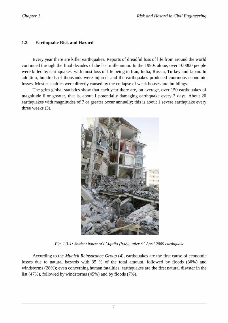
Fig. 1.3-1: Student house of L’Aquila (Italy), after 6th April 2009 earthquake
According to the Munich Reinsurance Group (4), earthquakes are the first cause of economic
losses due to natural hazards with 35 % of the total amount, followed by floods (30%) and
windstorms (28%); even concerning human fatalities, earthquakes are the first natural disaster in the
list (47%), followed by windstorms (45%) and by floods (7%).
Chapter 1 Risk and Hazard in Civil Engineering
8
Exposure is increasing due to the migration of population, goods and facilities into seismic-
hazardous areas (megacities built crossing active faults, buildings founded on soft soils, etc.). In
addition, always more challenging designs are realized (long-span bridges, high-rise buildings,
power plants, etc.) that requires that compliance of the soils and seismic effects along the interface
between the soil and the structure must be considered as carefully as possible.
Therefore the relevance of Soil-Structure Interaction (SSI) phenomena for a risk analysis is
absolutely evident, also given the economic and strategic importance of the aforementioned types of
structures.
As discussed in the previous section, in everyday speech, the nouns “risk” and “hazard” are
synonymous. By contrast, it is helpful in technical descriptions to give them distinct meanings.
Thus we define “hazard” the event itself, that is, the earthquake ground shaking; whereas “risk” is
the danger the hazard presents to vulnerable buildings or persons.
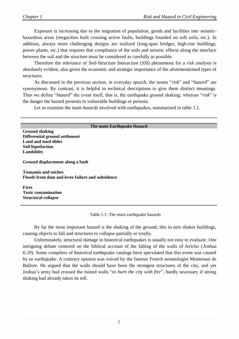
Let us examine the main hazards involved with earthquakes, summarized in table 1.1.
The main Earthquake Hazard
Ground shaking
Differential ground settlement
Land and mud slides
Soil liquefaction
Landslides
Ground displacement along a fault
Tsunamis and seiches
Floods from dam and levee failure and subsidence
Fires
Toxic contamination
Structural collapse
Table 1.1: The main earthquake hazards
By far the most important hazard is the shaking of the ground; this in turn shakes buildings,
causing objects to fall and structures to collapse partially or totally.
Unfortunately, structural damage in historical earthquakes is usually not easy to evaluate. One
intriguing debate centered on the biblical account of the falling of the walls of Jericho (Joshua
6:20). Some compilers of historical earthquake catalogs have speculated that this event was caused
by an earthquake. A contrary opinion was voiced by the famous French seismologist Montessus de
Ballore. He argued that the walls should have been the strongest structures of the city, and yet
Joshua’s army had crossed the ruined walls “to burn the city with fire”, hardly necessary if strong
shaking had already taken its toll.

Chapter 1 Risk and Hazard in Civil Engineering
9
For some major ancient historical earthquakes, the effects have been recorded in other ways.
For example, the damage resulting from one that struck Basel, Switzerland, on October 8, 1356, is
represented for posterity in a woodcut done two centuries later (fig. 1.3-2) or Rimini earthquake,
Italy, on December 25, 1789 was painted with holy representations (fig. 1.3-3).
Fig. 1.3-2: Artist’s impression of damage to Basel, Switzerland after the October 1356 earthquake,
shown on a woodcut from the “Basler Chronik” of Christian Wurstisen, 1580.
[From Basel und das Erdbeben von 1356, Basel: Rudolf Suter, 1956]
Fig. 1.3-3: Artist’s impression of Rimini earthquake, Italy. [after December 25, 1789 earthquake]

Chapter 1 Risk and Hazard in Civil Engineering
1 0
1.4 Contribution of the present research work
The importance of the nature of the sub-soil for the seismic response of structures has been
demonstrated in many earthquakes. For example, it is clear from studies of earthquakes that the
relationship between the periods of vibration of structures and the period of the supporting soil is
profoundly important regarding the seismic response of the structure.
As an example the Mexico earthquakes of 1957 and 1985 witnessed extensive damage to
long-period structures in the former lake bed area of Mexico City where the flexible lacustrine
deposits caused great amplification of long period waves (5), (6).
A more typical example of an earthquake where the fundamental period of structures which
were most damaged was closely related to depth of alluvium, was that in Caracas in 1967 (7).
Again, long-period structures were damaged in areas of greater depth of alluvium.
In the case of the 1970 earthquake at Gediz, Turkey, part of a factory was demolished in a
town 135 km from the epicenter while no other buildings in the town were damaged.
Subsequent investigations revealed that the fundamental period of vibration of the factory was
approximately equal to that of the underlying soil. Further evidence of the importance of periods of
vibration was derived from the medium-sized earthquake of Caracas in 1967, which completely
destroyed four buildings and caused extensive damage to many others. The pattern of structural
damage has been directly related to the depth of soft alluvium overlying the bedrock (7).
Extensive damage to medium-rise buildings (5–9 storeys) was reported in areas where depth
to bedrock was less than 100m while in areas where the alluvium thickness exceeded 150m the
damage was greater in taller buildings (over 14 storeys). The depth of alluvium is, of course,
directly related to the periods of vibration of the soil. (see par. 2.2.3).
To evaluate the seismic response of a structure at a given site, the dynamic properties of the
combined soil-structure system must be understood. The nature of the sub-soil may influence the
response of the structure in four ways:
(1) The seismic excitation at bedrock is modified during transmission through the overlying
soils to the foundation. This may cause attenuation or amplification effects.
(2) The fixed base dynamic properties of the structure may be significantly modified by the
presence of soils overlying bedrock. This will include changes in the mode shapes and
periods of vibration.
(3) A significant part of the vibrational energy of the flexibly supported structure may be
dissipated by material damping and radiation damping in the supporting medium.
(4) The increase in the fundamental period of moderately flexible structures due to soil-
structure interaction may have detrimental effects on the imposed seismic demand.
Chapter 1 Risk and Hazard in Civil Engineering
1 1
Items (2)–(4) above are investigated under the general title of soil-structure interaction, which
may be defined as the interdependent response relationship between a structure and its supporting
soil. The behavior of the structure is dependent in part upon the nature of the supporting soil, and
similarly, the behavior of the stratum is modified by the presence of the structure.
It follows that soil amplification and attenuation (item (1) above) will also be influenced by
the presence of the structure, as the effect of soil-structure interaction is to produce a difference
between the motion at the base of the structure and the free-field motion which would have
occurred at the same point in the absence of the structure.
In practice, however, this refinement in determining the soil amplification is seldom taken
into account, the free-field motion generally being that which is applied to the soil-structure model.
Because of the difficulties involved in making dynamic analytical models of soil systems, it has
been common practice to ignore soil-structure interaction effects simply treating structures as if
rigidly based regardless of the soil conditions.
However, intensive study in recent years has produced considerable advances in our
knowledge of soil-structure interaction effects and also in the analytical techniques available, as
discussed in the next chapter.
Concerning the large sphere of the risk management framework this research work focuses on
hazard assessment and structural vulnerability assessment, that is mainly on the step of Soil-
Structural Interaction (SSI) analysis in the process of risk analysis, which is the first step of risk
assessment, as defined in the previous paragraph.
The ambitious attempt of this work is to include Soil-Structure Interaction approach in risk
analysis.
Chapter 2 Dynamic Soil-Structure Interaction (SSI)
1 2
Chapter 2
Dynamic Soil-Structure Interaction (SSI)
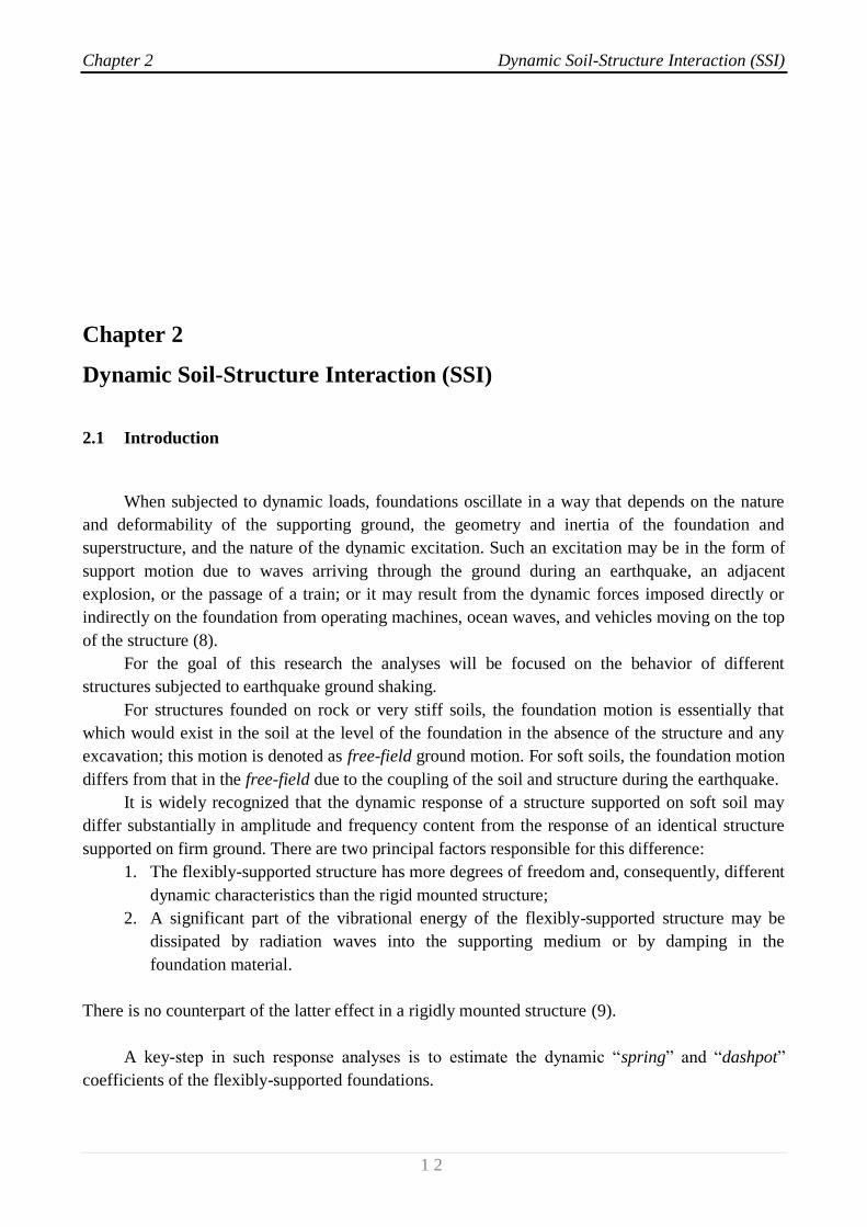
2.1 Introduction
When subjected to dynamic loads, foundations oscillate in a way that depends on the nature
and deformability of the supporting ground, the geometry and inertia of the foundation and
superstructure, and the nature of the dynamic excitation. Such an excitation may be in the form of
support motion due to waves arriving through the ground during an earthquake, an adjacent
explosion, or the passage of a train; or it may result from the dynamic forces imposed directly or
indirectly on the foundation from operating machines, ocean waves, and vehicles moving on the top
of the structure (8).
For the goal of this research the analyses will be focused on the behavior of different
structures subjected to earthquake ground shaking.
For structures founded on rock or very stiff soils, the foundation motion is essentially that
which would exist in the soil at the level of the foundation in the absence of the structure and any
excavation; this motion is denoted as free-field ground motion. For soft soils, the foundation motion
differs from that in the free-field due to the coupling of the soil and structure during the earthquake.
It is widely recognized that the dynamic response of a structure supported on soft soil may
differ substantially in amplitude and frequency content from the response of an identical structure
supported on firm ground. There are two principal factors responsible for this difference:
1. The flexibly-supported structure has more degrees of freedom and, consequently, different
dynamic characteristics than the rigid mounted structure;
2. A significant part of the vibrational energy of the flexibly-supported structure may be
dissipated by radiation waves into the supporting medium or by damping in the
foundation material.
There is no counterpart of the latter effect in a rigidly mounted structure (9).
A key-step in such response analyses is to estimate the dynamic “spring” and “dashpot”
coefficients of the flexibly-supported foundations.

Chapter 2 Dynamic Soil-Structure Interaction (SSI)
1 3
2.2 Complex stiffness matrix
Soil-Structure Interaction analyses are performed simplifying the general equation of motion
using an equivalent damping value ; thus the equation of motion
is transformed as
where
As a result a viscous damped system can be simplified as an undamped system with complex
stiffness.
The use of this approach is however restricted to harmonic excitations.
The phase error between the two responses is of no importance for practical problems.
Chapter 2 Dynamic Soil-Structure Interaction (SSI)
1 4
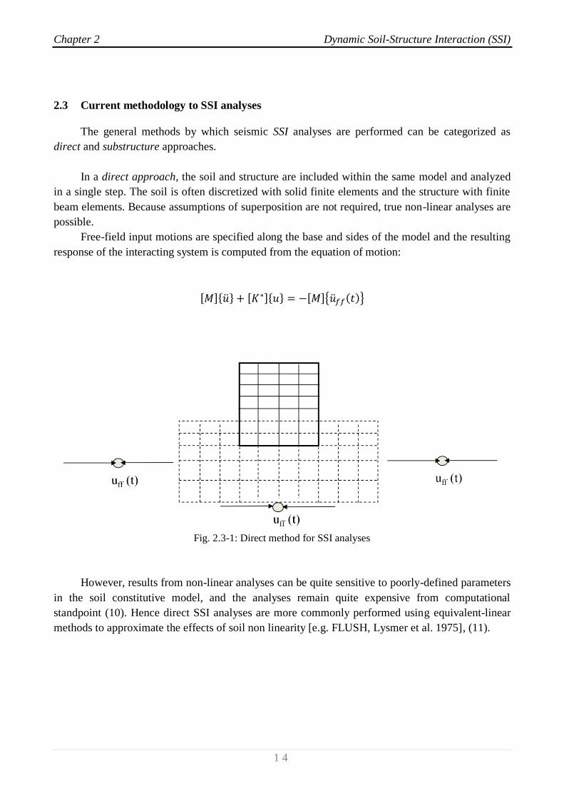
2.3 Current methodology to SSI analyses
The general methods by which seismic SSI analyses are performed can be categorized as
direct and substructure approaches.
In a direct approach, the soil and structure are included within the same model and analyzed
in a single step. The soil is often discretized with solid finite elements and the structure with finite
beam elements. Because assumptions of superposition are not required, true non-linear analyses are
possible.
Free-field input motions are specified along the base and sides of the model and the resulting
response of the interacting system is computed from the equation of motion:
Fig. 2.3-1: Direct method for SSI analyses
However, results from non-linear analyses can be quite sensitive to poorly-defined parameters
in the soil constitutive model, and the analyses remain quite expensive from computational
standpoint (10). Hence direct SSI analyses are more commonly performed using equivalent-linear
methods to approximate the effects of soil non linearity [e.g. FLUSH, Lysmer et al. 1975], (11).
Chapter 2 Dynamic Soil-Structure Interaction (SSI)
1 5
In a substructure approach the SSI problem is divided into three distinct parts which are
combined to formulate the complete solution. The superposition inherent to this approach requires
an assumption of linear soil and structure behavior.
Such approach may be applied even to moderately non-linear systems; it has been observed
(12) that in the case of flexible piles the deformations due to the lateral loading transmitted from the
superstructure attenuate very rapidly with depth (they practically vanish below the active length
which is of the order of 10 pile diameters below the ground surface). Therefore shear strains
induced in the soil due to inertial interaction may be significant only near the ground surface. By
contrast vertical S-waves induce displacements, curvatures and shear strains that are likely to be
important only at relatively deep elevations. Thus since soil strains are controlled by inertial effects
near the ground surface and by kinematic effects at greater depths the superposition may be
reasonable approximation even when non-linear soil behavior is expected.
The principal advantage of the substructure approach is its flexibility. Because each step is
independent of the others, the analyst can focus resources on the most significant aspects of the
problem; the primary causes of Soil-Structure Interaction can be isolated:
1. Kinematic Interaction (KI): inability of the foundation to match the free-field
deformation;
2. Inertial Interaction (II): Effect of the dynamic response of the structure-foundation
system on the movement of the supporting soil.
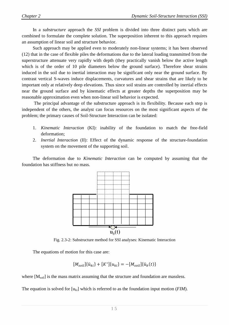
The deformation due to Kinematic Interaction can be computed by assuming that the
foundation has stiffness but no mass.
Fig. 2.3-2: Substructure method for SSI analyses: Kinematic Interaction
The equations of motion for this case are:
where [Msoil] is the mass matrix assuming that the structure and foundation are massless.
The equation is solved for [uki] which is referred to as the foundation input motion (FIM).
Chapter 2 Dynamic Soil-Structure Interaction (SSI)
1 6
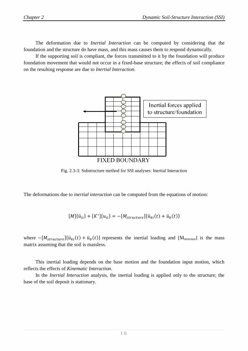
The deformation due to Inertial Interaction can be computed by considering that the
foundation and the structure do have mass, and this mass causes them to respond dynamically.
If the supporting soil is compliant, the forces transmitted to it by the foundation will produce
foundation movement that would not occur in a fixed-base structure; the effects of soil compliance
on the resulting response are due to Inertial Interaction.
Fig. 2.3-3: Substructure method for SSI analyses: Inertial Interaction
The deformations due to inertial interaction can be computed from the equations of motion:
where represents the inertial loading and [Mstructure] is the mass
matrix assuming that the soil is massless.
This inertial loading depends on the base motion and the foundation input motion, which
reflects the effects of Kinematic Interaction.
In the Inertial Interaction analysis, the inertial loading is applied only to the structure; the
base of the soil deposit is stationary.
Chapter 2 Dynamic Soil-Structure Interaction (SSI)
1 7
Given the above formulations a general procedure for the substructure approach can be
developed:
1. A Kinematic Interaction analysis, in which the foundation-structure system is assumed
to have stiffness but no mass, is performed.
The motion derived from Kinematic Interaction analysis is combined with the base
motion to produce the total kinematic motion of the foundation-structure system:
foundation input motion.
2. The Foundation Input Motion is used to apply inertial loads to the structure in an
Inertial Interaction analysis, in which the soil, the foundation and the structure are all
assumed to have stiffness and mass.
Combining the two previous equations we obtain:
Since and
The previous equation is equivalent to the original equation of motion:

Chapter 2 Dynamic Soil-Structure Interaction (SSI)
1 8
2.4 Kinematic and Inertial Interaction
During earthquake shaking, soil deforms under the influence of the incident seismic waves
and “carries” dynamically with it the foundation and the supported structure. In turn, the induced
motion of the superstructure generates inertial forces which result in dynamic stresses at the
foundation that are transmitted into the supporting soil. Thus, superstructure-induced deformations
develop in the soil while additional waves emanate from the soil-structure interface. In response,
foundation and superstructure undergo further dynamic displacements, which generate further
inertial forces and so on (13).
The above phenomena occur simultaneously, however it is convenient to separate them into
two successive phenomena referred as “kinematic interaction” and “inertial interaction” (14) (15)
(16) (17), and obtain the response of the soil-foundation-structure system as a superposition of these
two interaction effects (13).
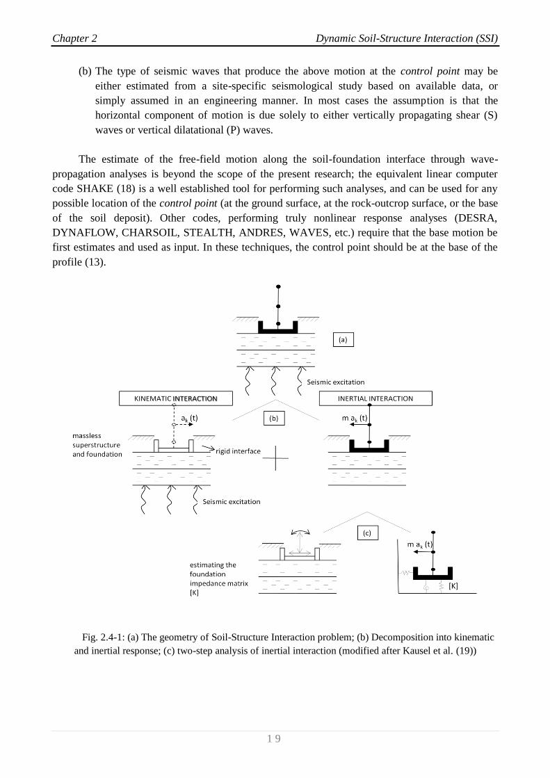
1. Kinematic Interaction (KI) refers to the effects of the incident seismic waves to the system
shown in Fig. 2.4-1b, which consists essentially of the foundation and the supporting soil,
with the mass of the superstructure set equal to zero (in contrast with the complete system
of Fig. 2.4.1a). The main consequence of KI is that it leads to a “foundation input motion”
(FIM) which is different (usually smaller) than the motion of the free-field soil and, in
addition, contains a rotational component. The difference could be significant for
embedded foundations.
2. Inertial Interaction (II) refers to the response of the complete soil-foundation-structure
system to the excitation by D’Alembert forces associated with the acceleration of the
superstructure due to the KI (Fig. 2.4-1b).
Furthermore, for a surface or embedded foundation, II analysis is also conveniently
performed in two steps, as shown in Fig. 2.4-1c: first compute the foundation dynamic
impedance (springs and dashpots) associated with each mode of vibration, and then
determine the seismic response of the structure and foundation supported on these springs
and dashpots, and subjected to the kinematic accelerations ak (t) of the base.
2.4.1 Assessing the effects of Kinematic Interaction
The first step of the KI analysis is to determine the free-field response of the site, that is, the
spatial and temporal variation of the ground motion before building the structure (13). This task
requires that:
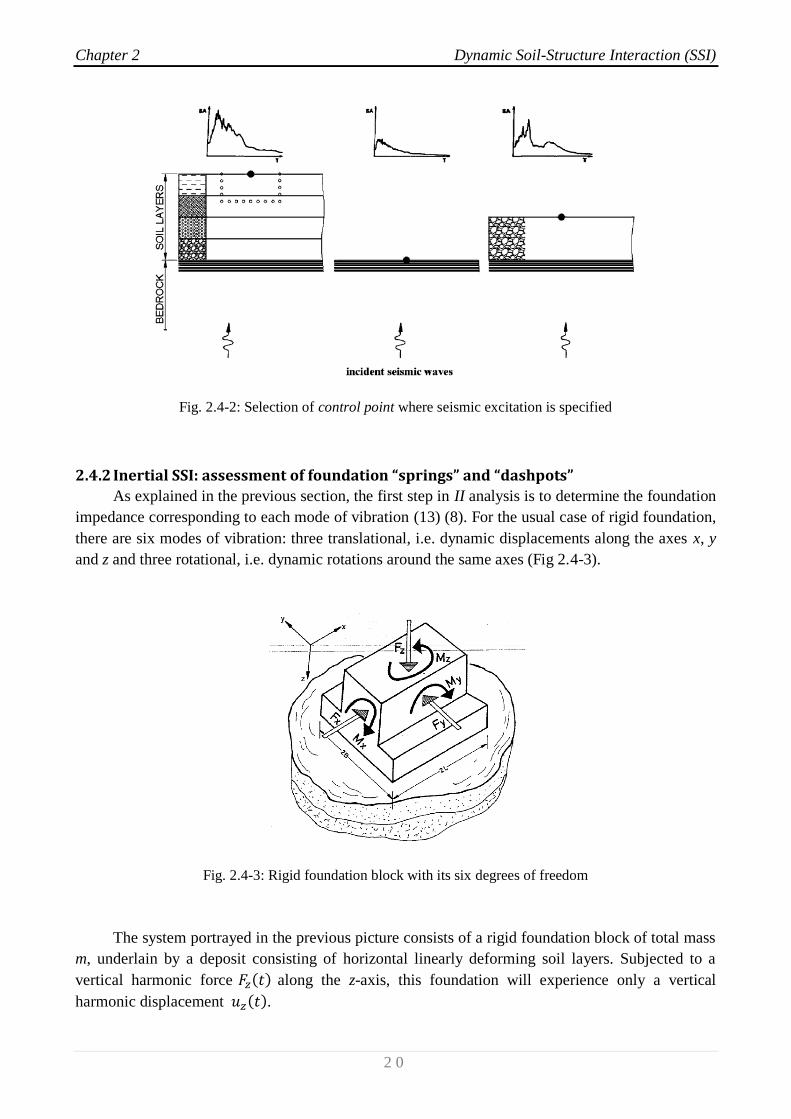
(a) The design motion must be known at a specific control point, which is usually taken at the
ground surface or at the rock-outcrop surface, as shown in Fig. 2.4-2. Most frequently the
design motion is given in the form of a design response spectrum in the horizontal
direction and sometimes also in the vertical direction.
Chapter 2 Dynamic Soil-Structure Interaction (SSI)
1 9
(b) The type of seismic waves that produce the above motion at the control point may be
either estimated from a site-specific seismological study based on available data, or
simply assumed in an engineering manner. In most cases the assumption is that the
horizontal component of motion is due solely to either vertically propagating shear (S)
waves or vertical dilatational (P) waves.
The estimate of the free-field motion along the soil-foundation interface through wave-
propagation analyses is beyond the scope of the present research; the equivalent linear computer
code SHAKE (18) is a well established tool for performing such analyses, and can be used for any
possible location of the control point (at the ground surface, at the rock-outcrop surface, or the base
of the soil deposit). Other codes, performing truly nonlinear response analyses (DESRA,
DYNAFLOW, CHARSOIL, STEALTH, ANDRES, WAVES, etc.) require that the base motion be
first estimates and used as input. In these techniques, the control point should be at the base of the
profile (13).
Fig. 2.4-1: (a) The geometry of Soil-Structure Interaction problem; (b) Decomposition into kinematic
and inertial response; (c) two-step analysis of inertial interaction (modified after Kausel et al. (19))
Chapter 2 Dynamic Soil-Structure Interaction (SSI)
2 0
Fig. 2.4-2: Selection of control point where seismic excitation is specified
2.4.2 Inertial SSI: assessment of foundation “springs” and “dashpots”
As explained in the previous section, the first step in II analysis is to determine the foundation
impedance corresponding to each mode of vibration (13) (8). For the usual case of rigid foundation,
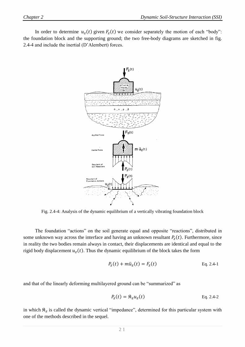
there are six modes of vibration: three translational, i.e. dynamic displacements along the axes x, y
and z and three rotational, i.e. dynamic rotations around the same axes (Fig 2.4-3).
Fig. 2.4-3: Rigid foundation block with its six degrees of freedom
The system portrayed in the previous picture consists of a rigid foundation block of total mass
m, underlain by a deposit consisting of horizontal linearly deforming soil layers. Subjected to a
vertical harmonic force along the z-axis, this foundation will experience only a vertical
harmonic displacement .
Chapter 2 Dynamic Soil-Structure Interaction (SSI)
2 1
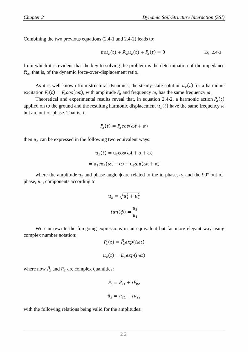
In order to determine given we consider separately the motion of each “body”:
the foundation block and the supporting ground; the two free-body diagrams are sketched in fig.
2.4-4 and include the inertial (D’Alembert) forces.
Fig. 2.4-4: Analysis of the dynamic equilibrium of a vertically vibrating foundation block
The foundation “actions” on the soil generate equal and opposite “reactions”, distributed in
some unknown way across the interface and having an unknown resultant . Furthermore, since
in reality the two bodies remain always in contact, their displacements are identical and equal to the
rigid body displacement . Thus the dynamic equilibrium of the block takes the form
Eq. 2.4-1
and that of the linearly deforming multilayered ground can be “summarized” as
Eq. 2.4-2
in which is called the dynamic vertical “impedance”, determined for this particular system with
one of the methods described in the sequel.
Chapter 2 Dynamic Soil-Structure Interaction (SSI)
2 2
Combining the two previous equations (2.4-1 and 2.4-2) leads to:
Eq. 2.4-3
from which it is evident that the key to solving the problem is the determination of the impedance
, that is, of the dynamic force-over-displacement ratio.
As it is well known from structural dynamics, the steady-state solution for a harmonic
excitation , with amplitude and frequency , has the same frequency .
Theoretical and experimental results reveal that, in equation 2.4-2, a harmonic action
applied on to the ground and the resulting harmonic displacement have the same frequency
but are out-of-phase. That is, if
then can be expressed in the following two equivalent ways:
where the amplitude and phase angle are related to the in-phase, and the 90°-out-of-
phase, , components according to
We can rewrite the foregoing expressions in an equivalent but far more elegant way using
complex number notation:
where now and are complex quantities:
with the following relations being valid for the amplitudes:
Chapter 2 Dynamic Soil-Structure Interaction (SSI)
2 3
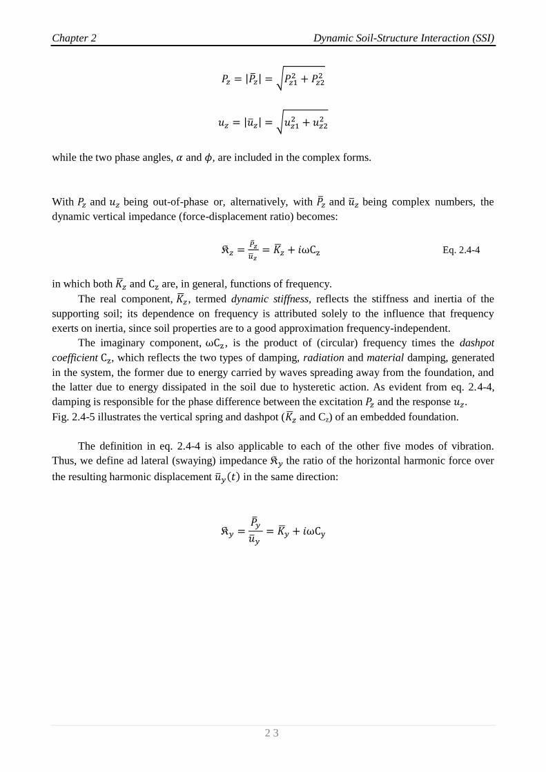
while the two phase angles, and , are included in the complex forms.
With and being out-of-phase or, alternatively, with and being complex numbers, the
dynamic vertical impedance (force-displacement ratio) becomes:
Eq. 2.4-4
in which both and are, in general, functions of frequency.
The real component, , termed dynamic stiffness, reflects the stiffness and inertia of the
supporting soil; its dependence on frequency is attributed solely to the influence that frequency
exerts on inertia, since soil properties are to a good approximation frequency-independent.
The imaginary component, , is the product of (circular) frequency times the dashpot
coefficient , which reflects the two types of damping, radiation and material damping, generated
in the system, the former due to energy carried by waves spreading away from the foundation, and
the latter due to energy dissipated in the soil due to hysteretic action. As evident from eq. 2.4-4,
damping is responsible for the phase difference between the excitation and the response .
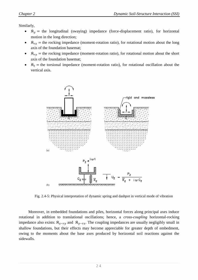
Fig. 2.4-5 illustrates the vertical spring and dashpot ( and Cz) of an embedded foundation.
The definition in eq. 2.4-4 is also applicable to each of the other five modes of vibration.
Thus, we define ad lateral (swaying) impedance the ratio of the horizontal harmonic force over
the resulting harmonic displacement in the same direction:
Chapter 2 Dynamic Soil-Structure Interaction (SSI)
2 4
Similarly,
the longitudinal (swaying) impedance (force-displacement ratio), for horizontal
motion in the long direction;
the rocking impedance (moment-rotation ratio), for rotational motion about the long
axis of the foundation basemat;
the rocking impedance (moment-rotation ratio), for rotational motion about the short
axis of the foundation basemat;
the torsional impedance (moment-rotation ratio), for rotational oscillation about the
vertical axis.
Fig. 2.4-5: Physical interpretation of dynamic spring and dashpot in vertical mode of vibration
Moreover, in embedded foundations and piles, horizontal forces along principal axes induce
rotational in addition to translational oscillations; hence, a cross-coupling horizontal-rocking
impedance also exists: and . The coupling impedances are usually negligibly small in
shallow foundations, but their effects may become appreciable for greater depth of embedment,
owing to the moments about the base axes produced by horizontal soil reactions against the
sidewalls.
Chapter 2 Dynamic Soil-Structure Interaction (SSI)
2 5
2.4.3 Computing dynamic impedances
The most important geometric and material factors affecting the dynamic impedance of a
foundation are:
1. the foundation shape (circular, strip, rectangular, arbitrary);
2. the type of soil profile (deep uniform or multi-layer deposit, shallow stratum on rock);
3. the embedment (surface foundation, embedded foundation, pile foundation).
For a project of critical significance a case-specific analysis must be performed, using the
most suitable numerical computer program. In most practical cases, however, foundation
impedances can be estimated from approximate expressions and charts. For the usual case of a
practically rigid foundation, a number of analytical formulae and charts for such stiffnesses have
been published (e.g. (8), (20), (21), (22), (23), (24), (25), (26), (27)); such charts and tables are not
presented in the present work.
All the formulae developed give:
the dynamic stiffness (“springs”), as a product of static stiffness, K, and
dynamic stiffness coefficient :
the radiation damping (“dashpot”) coefficient . These coefficients do not
include the soil hysteretic damping . To incorporate such damping, one should
simply add to the foregoing value the corresponding material dashpot coefficient
:
total = radiation +
Natural soil deposits are frequently underlain by very stiff material or bedrock at a shallow
depth (H), rather than extending to practically infinite depth as the homogeneous halfspace implies.
The proximity of such stiff formation to the oscillating surface modifies the static stiffness, , and
dashpot coefficients . In particular, the static stiffnesses in all modes decrease with the relative
depth to bedrock H/B (with B characteristic length of the foundation).
Particularly sensitive to variations in the depth to rock are the vertical stiffnesses; apparently
when a rigid foundation extends into the zone of influence of a particular loading mode, it
eliminates the corresponding deformations and thereby increases the stiffness.

Chapter 2 Dynamic Soil-Structure Interaction (SSI)
2 6
The variation of the dynamic stiffness coefficients with frequency reveals an equally strong
dependence on the depth to bedrock H/B. on a stratum, is not a smooth function but exhibits
undulations (peaks and valleys) associated with the natural frequencies (in shearing and
compression-extension) of the stratum. In other words, the observed fluctuations are the outcome of
resonance phenomena: waves emanating from the oscillating foundation reflect at the soil-bedrock
interface and return back to their source at the surface. As a result, the amplitude of the foundation
motion may significantly increase at frequencies near the natural frequencies of the deposit. Thus,
the dynamic stiffness (being the inverse of displacements) exhibits troughs, which can be very steep
when the hysteretic damping of the soil is small (in fact, in certain cases, would be exactly
zero if the soil was ideally elastic).
For the shearing modes of vibration (swaying and torsion) the natural fundamental frequency
of the stratum which controls the behavior of is
where H denotes the thickness of the layer, while for the compressing modes (vertical and
rocking) the corresponding frequency is
The variation of the dashpot coefficient, , with frequency reveals a twofold effect on the
presence of a rigid base at relatively shallow depth. First, also exhibits undulations (crests and
troughs) due to wave reflections at the rigid boundary, but they are not as significant as for the
corresponding stiffness . Second, and far more important from a practical point of view, is that
at low frequencies below the first resonant (cutoff) frequency of each mode of vibration, radiation
damping is zero or negligible for all shapes of footings and all modes of vibration. This is due to the
fact that no surface waves can exist in a soil stratum over bedrock at such frequencies; and, since
the bedrock also prevents waves from propagating downward, the overall radiation of wave energy
from the footing is negligible or nonexistent.
Such an elimination of radiation damping may have severe consequences for heavy
foundations oscillating vertically or horizontally, which would have experienced substantial
amounts of damping in a very deep deposit (halfspace). On the other hand, since the low-frequency
values of in rocking and torsion are small even in a halfspace, operating below the cutoff
frequencies may not change appreciably from the presence of bedrock. At operating frequencies f
beyond fs or fc, as appropriate for each mode, the “stratum” damping fluctuates about the halfspace
damping (H/B = ).

Chapter 2 Dynamic Soil-Structure Interaction (SSI)
2 7
m
r
m
2.5 Effect of SSI
The classical approach for elastodynamic analysis of Soil-Structure Interaction aims at
replacing the actual structure by an equivalent simple oscillator supported on a set of frequency-
dependent springs and dashpots accounting for the stiffness and damping of the soil medium. This
model has been adopted by several researchers, including Parmalee (1967), Veletsos et al. (1974,
1975, 1977), Jennings & Bielak (1973), Wolf (1985) and, more recently, Aviles et al. (1996, 1998).
The system studied is shown in Fig. 2.5-1. It involves a simple oscillator on flexible base
representing a single storey structure, or a multi storey structure after a pertinent reduction of its
degrees-of-freedom (e.g., considering that the mass is concentrated at the point where the resultant
inertial force acts (28).
(a) (b)
Fig. 2.5.-1: (a) Structure idealized by a stick model, (b) Reduced single degree-of-freedom model
The structure is described by its stiffness k, mass m, height h, and damping ratio , which may
be either viscous or linearly hysteretic. The foundation consists of a rigid surface circular footing of
radius r resting on a homogeneous, linearly elastic, isotropic halfspace described by a shear
modulus Gs, mass density s, Poisson’s ratio s, and hysteretic damping ratio s. foundation stiffness
is modeled by frequency-dependent springs and representing stiffness in translational and
rocking oscillations respectively. To ensure uniform units in all stiffness terms, is expressed by a
translational vertical spring acting at distance r from the center of the footing (29).
Damping is modeled by a pair of dashpots and , attached in parallel to the springs,
representing energy loss due to hysteretic action and wave radiation in the soil medium. In the
present formulation, the influence of foundation embedment and foundation mass is neglected.
h
k,
Chapter 2 Dynamic Soil-Structure Interaction (SSI)
2 8
m
r
The fixed-base frequency of the structure is denotes as s and represents its hysteretic
damping ratio:
The dynamic impedance along any degree of freedom of the system is defined
according to the formula:
in which is the real part of the impedance, C is the corresponding imaginary part, is the
cyclic excitation frequency, and . is the energy loss parameter, analogous (yet not
identical) to the viscous damping coefficient of a simple oscillator.
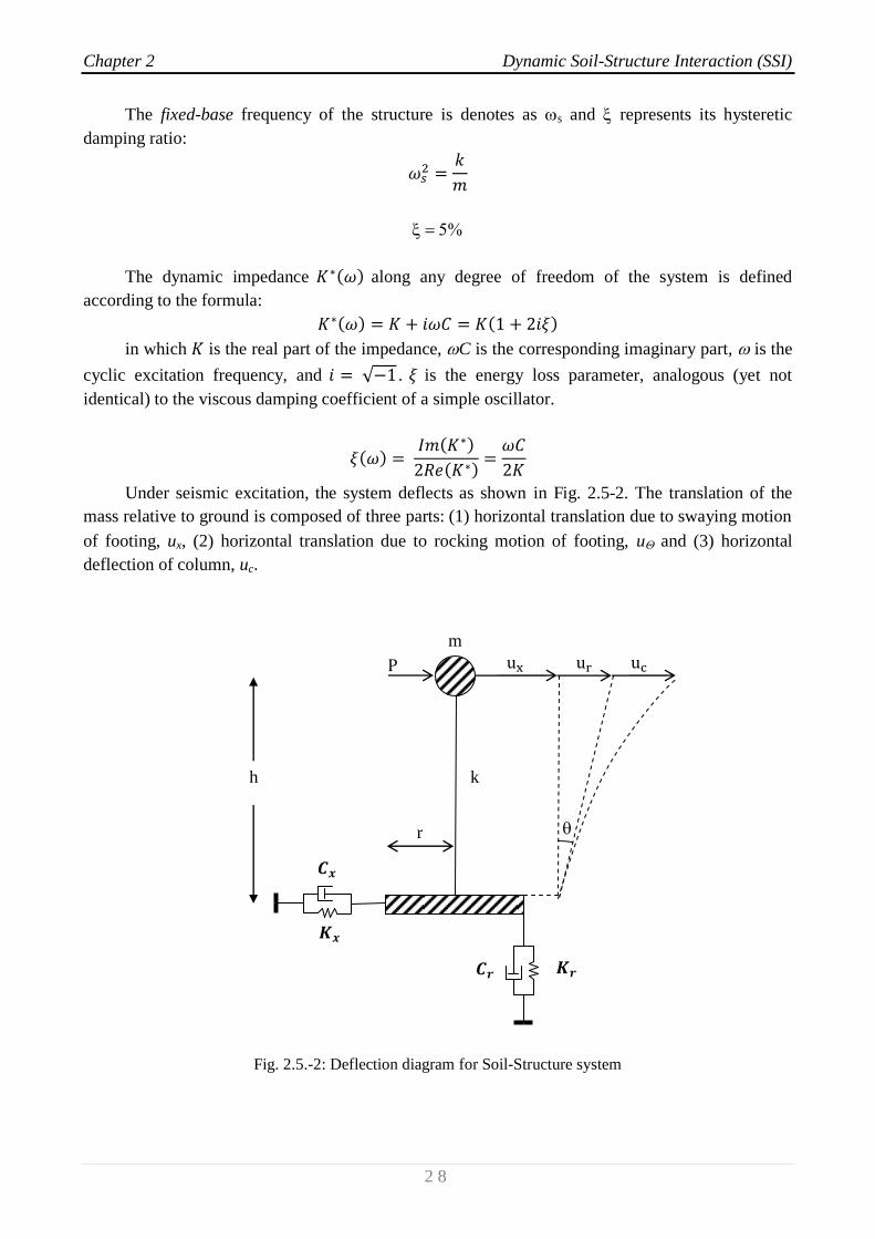
Under seismic excitation, the system deflects as shown in Fig. 2.5-2. The translation of the
mass relative to ground is composed of three parts: (1) horizontal translation due to swaying motion
of footing, ux, (2) horizontal translation due to rocking motion of footing, u and (3) horizontal
deflection of column, uc.
Fig. 2.5.-2: Deflection diagram for Soil-Structure system
h
k
Chapter 2 Dynamic Soil-Structure Interaction (SSI)
2 9
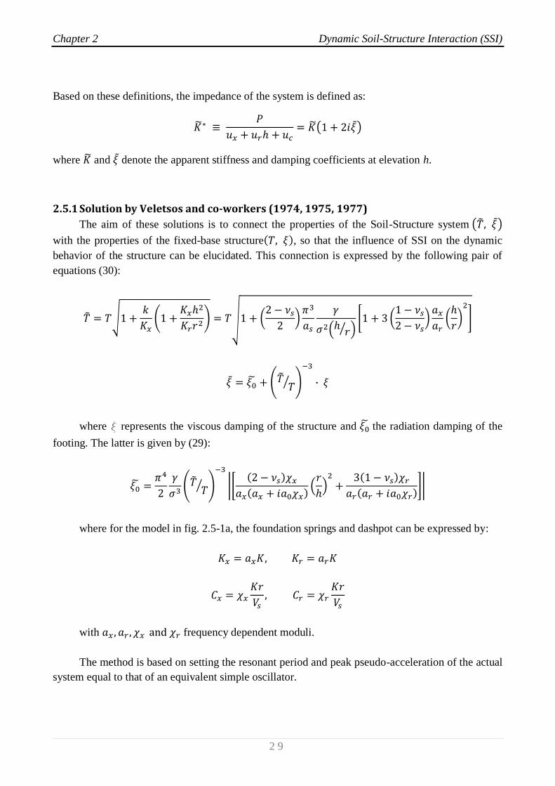
Based on these definitions, the impedance of the system is defined as:
where and denote the apparent stiffness and damping coefficients at elevation h.
2.5.1 Solution by Veletsos and co-workers (1974, 1975, 1977)
The aim of these solutions is to connect the properties of the Soil-Structure system
with the properties of the fixed-base structure , so that the influence of SSI on the dynamic
behavior of the structure can be elucidated. This connection is expressed by the following pair of
equations (30):
where x represents the viscous damping of the structure and the radiation damping of the
footing. The latter is given by (29):
where for the model in fig. 2.5-1a, the foundation springs and dashpot can be expressed by:
with frequency dependent moduli.
The method is based on setting the resonant period and peak pseudo-acceleration of the actual
system equal to that of an equivalent simple oscillator.
Chapter 2 Dynamic Soil-Structure Interaction (SSI)
3 0
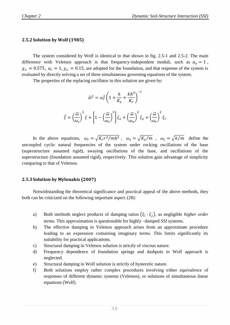
2.5.2 Solution by Wolf (1985)
The system considered by Wolf is identical to that shown in fig. 2.5-1 and 2.5-2. The main
difference with Veletsos approach is that frequency-independent moduli, such as ,
, , , are adopted for the foundation, and that response of the system is
evaluated by directly solving a set of three simultaneous governing equations of the system.
The properties of the replacing oscillator in this solution are given by:
In the above equations, , , define the
uncoupled cyclic natural frequencies of the system under rocking oscillations of the base
(superstructure assumed rigid), swaying oscillations of the base, and oscillations of the
superstructure (foundation assumed rigid), respectively. This solution gain advantage of simplicity
comparing to that of Veletsos.
2.5.3 Solution by Mylonakis (2007)
Notwithstanding the theoretical significance and practical appeal of the above methods, they
both can be criticized on the following important aspect (28):
a) Both methods neglect products of damping ratios , as negligible higher order
terms. This approximation is questionable for highly –damped SSI systems.
b) The effective damping in Veletsos approach arises from an approximate procedure
leading to an expression containing imaginary terms. This limits significantly its
suitability for practical applications.
c) Structural damping in Veletsos solution is strictly of viscous nature.
d) Frequency dependence of foundation springs and dashpots in Wolf approach is
neglected.
e) Structural damping in Wolf solution is strictly of hysteretic nature.
f) Both solutions employ rather complex procedures involving either equivalence of
responses of different dynamic systems (Veletsos), or solutions of simultaneous linear
equations (Wolf).
Chapter 2 Dynamic Soil-Structure Interaction (SSI)
3 1
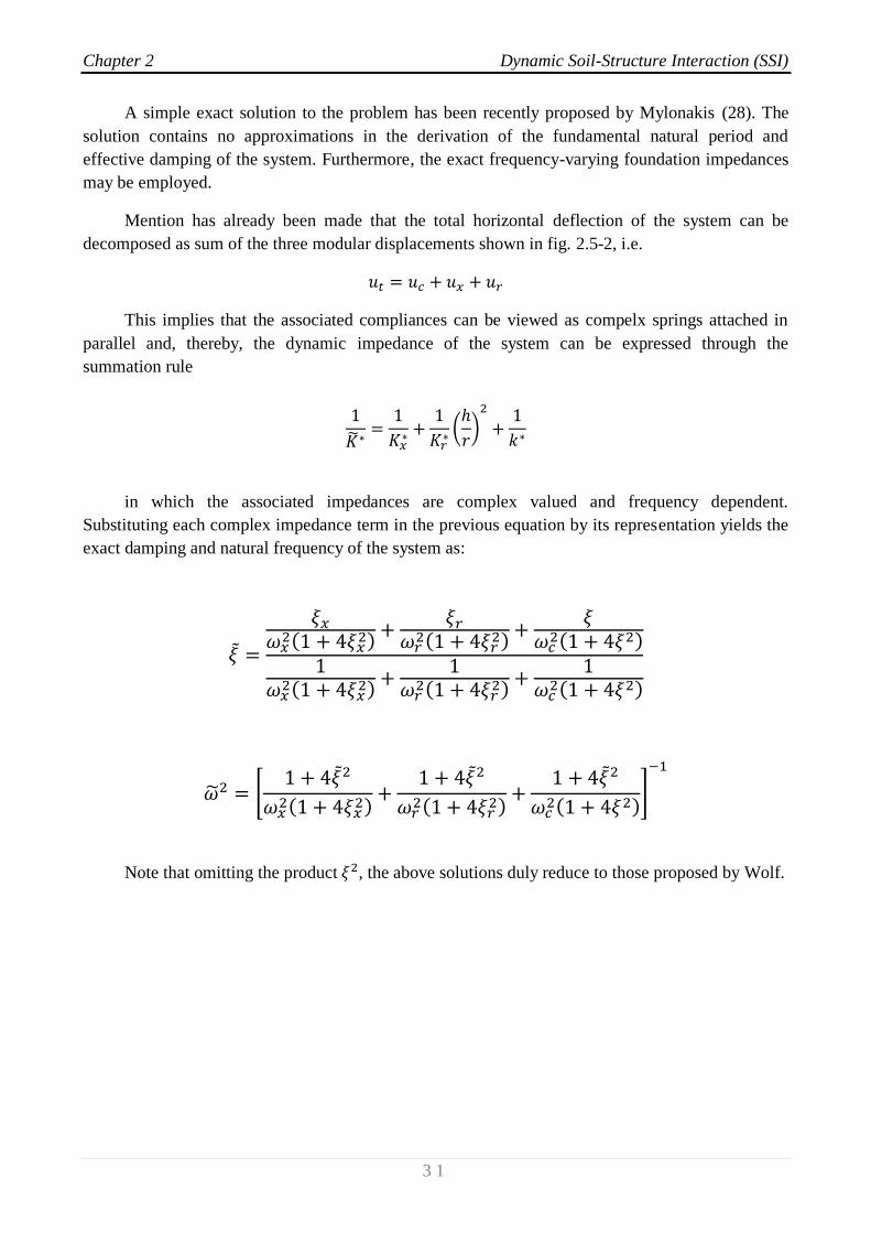
A simple exact solution to the problem has been recently proposed by Mylonakis (28). The
solution contains no approximations in the derivation of the fundamental natural period and
effective damping of the system. Furthermore, the exact frequency-varying foundation impedances
may be employed.
Mention has already been made that the total horizontal deflection of the system can be
decomposed as sum of the three modular displacements shown in fig. 2.5-2, i.e.
This implies that the associated compliances can be viewed as compelx springs attached in
parallel and, thereby, the dynamic impedance of the system can be expressed through the
summation rule
in which the associated impedances are complex valued and frequency dependent.
Substituting each complex impedance term in the previous equation by its representation yields the
exact damping and natural frequency of the system as:
Note that omitting the product , the above solutions duly reduce to those proposed by Wolf.
Chapter 2 Dynamic Soil-Structure Interaction (SSI)
3 2
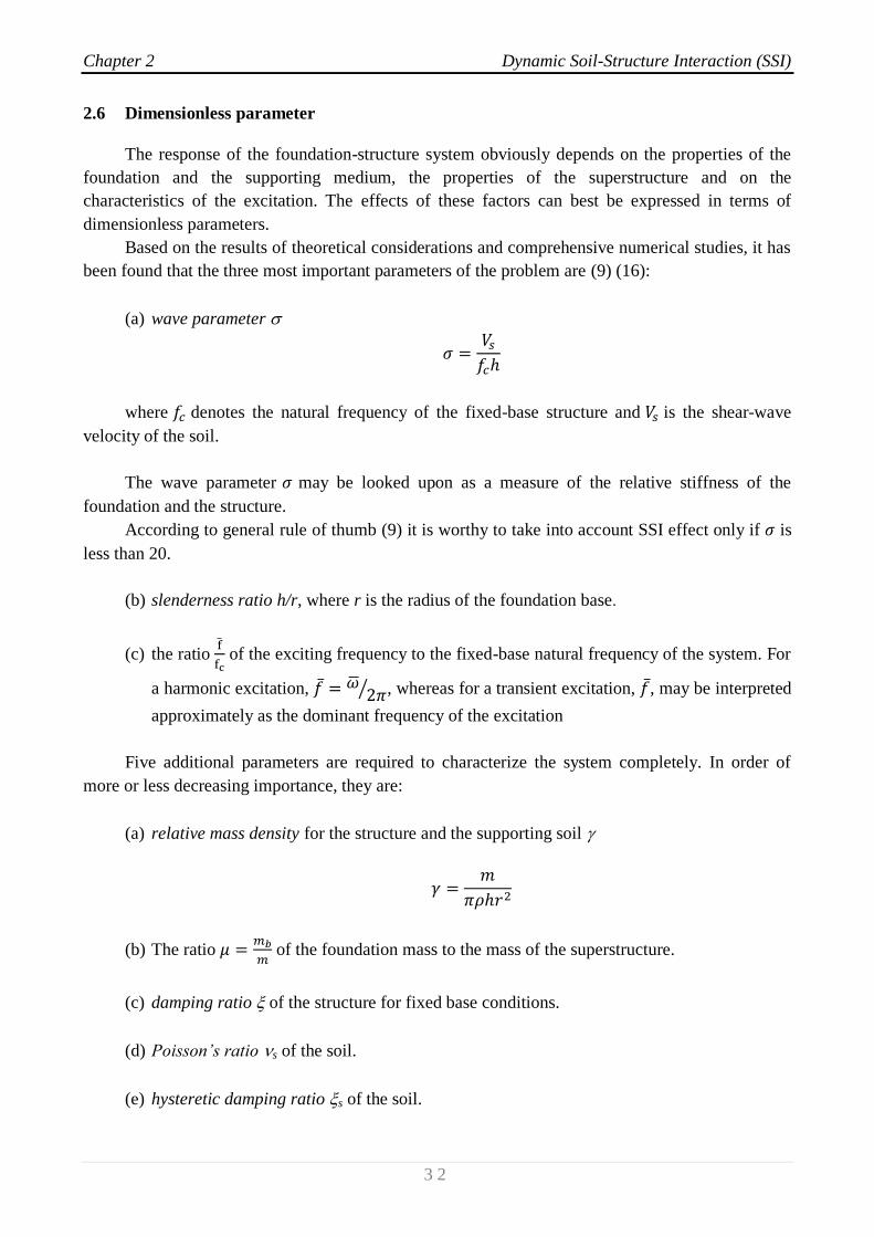
2.6 Dimensionless parameter
The response of the foundation-structure system obviously depends on the properties of the
foundation and the supporting medium, the properties of the superstructure and on the
characteristics of the excitation. The effects of these factors can best be expressed in terms of
dimensionless parameters.
Based on the results of theoretical considerations and comprehensive numerical studies, it has
been found that the three most important parameters of the problem are (9) (16):
(a) wave parameter
where denotes the natural frequency of the fixed-base structure and is the shear-wave
velocity of the soil.
The wave parameter may be looked upon as a measure of the relative stiffness of the
foundation and the structure.
According to general rule of thumb (9) it is worthy to take into account SSI effect only if is
less than 20.
(b) slenderness ratio h/r, where r is the radius of the foundation base.
(c) the ratio
of the exciting frequency to the fixed-base natural frequency of the system. For
a harmonic excitation, , whereas for a transient excitation, , may be interpreted
approximately as the dominant frequency of the excitation
Five additional parameters are required to characterize the system completely. In order of
more or less decreasing importance, they are:
(a) relative mass density for the structure and the supporting soil
(b) The ratio
of the foundation mass to the mass of the superstructure.
(c) damping ratio of the structure for fixed base conditions.
(d) Poisson’s ratio s of the soil.
(e) hysteretic damping ratio s of the soil.

Chapter 2 Dynamic Soil-Structure Interaction (SSI)
3 3
Classical solutions have been calculated taking , a representative value for buildings;
the foundation mass is considered to be negligible in comparison to the mass of the superstructure;
is taken as 0.45; and is taken as 5%. Within the ranges of interest in practical applications, the
response of the structure is found to be generally insensitive to variations in these particular
parameters.
Solutions are finally presented as function of a dimensionless frequency parameter, a0, which
has the form:
For practical applications in earthquake engineering, dimensionless frequencies in the range
0 ≤ ≤ 2 are usually considered. Values greater than 2 are far from typical frequencies generated
during earthquake shakings.
Chapter 2 Dynamic Soil-Structure Interaction (SSI)
3 4
2.7 SSI – Beneficial or detrimental?
The first objective of the paragraph is to evaluate the approach seismic regulations propose
for assessing SSI effects. This is done in two parts: (a) by examining the effects of SSI on the
response of elastic single-degree-of-freedom (SDOF) oscillators; and (b) by examining the effects
of increase in period due to SSI on the ductility demand imposed on elastoplastic SDOF oscillators.
The second objective is to assess SSI effects, exploring its role on the ductility of soil-
foundation-structure systems, determining (c) the ductility capacity factor and (d) the corresponding
ductility demand imposed on such systems founded on soft soil, during strong earthquake motion.
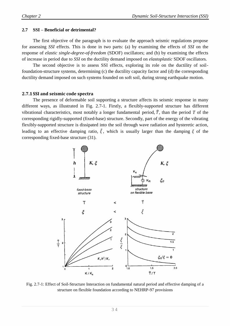
2.7.1 SSI and seismic code spectra
The presence of deformable soil supporting a structure affects its seismic response in many
different ways, as illustrated in Fig. 2.7-1. Firstly, a flexibly-supported structure has different
vibrational characteristics, most notably a longer fundamental period, , than the period T of the
corresponding rigidly-supported (fixed-base) structure. Secondly, part of the energy of the vibrating
flexibly-supported structure is dissipated into the soil through wave radiation and hysteretic action,
leading to an effective damping ratio, , which is usually larger than the damping of the
corresponding fixed-base structure (31).
Fig. 2.7-1: Effect of Soil-Structure Interaction on fundamental natural period and effective damping of a
structure on flexible foundation according to NEHRP-97 provisions
K, K,
h
Chapter 2 Dynamic Soil-Structure Interaction (SSI)
3 5
The seismic design of structures supported on deformable ground must properly account for
such an increase in fundamental period and damping.
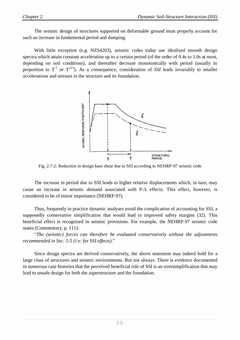
With little exception (e.g. NZS4203), seismic codes today use idealized smooth design
spectra which attain constant acceleration up to a certain period (of the order of 0.4s to 1.0s at most,
depending on soil conditions), and thereafter decrease monotonically with period (usually in
proportion to T-1
or T-2/3
). As a consequence, consideration of SSI leads invariably to smaller
accelerations and stresses in the structure and its foundation.
Fig. 2.7-2: Reduction in design base shear due to SSI according to NEHRP-97 seismic code
The increase in period due to SSI leads to higher relative displacements which, in turn, may
cause an increase in seismic demand associated with P- effects. This effect, however, is
considered to be of minor importance (NEHRP-97).
Thus, frequently in practice dynamic analyses avoid the complication of accounting for SSI, a
supposedly conservative simplification that would lead to improved safety margins (32). This
beneficial effect is recognized in seismic provisions. For example, the NEHRP-97 seismic code
states (Commentary, p. 111):
“The (seismic) forces can therefore be evaluated conservatively without the adjustments
recommended in Sec: 5:5 (i:e: for SSI effects)."
Since design spectra are derived conservatively, the above statement may indeed hold for a
large class of structures and seismic environments. But not always. There is evidence documented
in numerous case histories that the perceived beneficial role of SSI is an oversimplification that may
lead to unsafe design for both the superstructure and the foundation.
Chapter 2 Dynamic Soil-Structure Interaction (SSI)
3 6
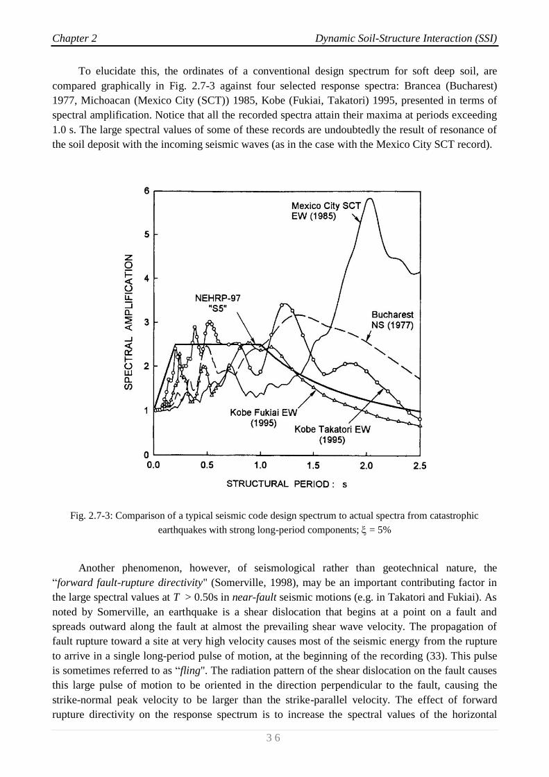
To elucidate this, the ordinates of a conventional design spectrum for soft deep soil, are
compared graphically in Fig. 2.7-3 against four selected response spectra: Brancea (Bucharest)
1977, Michoacan (Mexico City (SCT)) 1985, Kobe (Fukiai, Takatori) 1995, presented in terms of
spectral amplification. Notice that all the recorded spectra attain their maxima at periods exceeding
1.0 s. The large spectral values of some of these records are undoubtedly the result of resonance of
the soil deposit with the incoming seismic waves (as in the case with the Mexico City SCT record).
Fig. 2.7-3: Comparison of a typical seismic code design spectrum to actual spectra from catastrophic
earthquakes with strong long-period components; = 5%
Another phenomenon, however, of seismological rather than geotechnical nature, the
“forward fault-rupture directivity" (Somerville, 1998), may be an important contributing factor in
the large spectral values at T > 0.50s in near-fault seismic motions (e.g. in Takatori and Fukiai). As
noted by Somerville, an earthquake is a shear dislocation that begins at a point on a fault and
spreads outward along the fault at almost the prevailing shear wave velocity. The propagation of
fault rupture toward a site at very high velocity causes most of the seismic energy from the rupture
to arrive in a single long-period pulse of motion, at the beginning of the recording (33). This pulse
is sometimes referred to as “fling". The radiation pattern of the shear dislocation on the fault causes
this large pulse of motion to be oriented in the direction perpendicular to the fault, causing the
strike-normal peak velocity to be larger than the strike-parallel velocity. The effect of forward
rupture directivity on the response spectrum is to increase the spectral values of the horizontal

Chapter 2 Dynamic Soil-Structure Interaction (SSI)
3 7
component normal to the fault strike at periods longer than about 0.5s. Examples of this effect are
the Kobe (1995) JMA, Fukiai, Takatori, and Kobe University records; the Northridge (1994)
Rinaldi, Newhall, Sylmar Converter, and Sylmar Olive View records; the Landers (1992) Lucerne
Valley record, and many others. Fig. 2.7-4 shows the effects of rupture directivity in the time
history and response spectrum of the Rinaldi record of the 1994 Northridge earthquake.
Fig. 2.7-4: Acceleration and velocity time histories for the strike-normal and strike-parallel horizontal
components of ground motion, and their 5% damped response spectra, recorded at Rinaldi during the 1994
Northbridge earthquake. Note the pronounced high velocity/long period pulse in the fault-normal component
(after Somerville, 1998).
Evidently, records with enhanced spectral ordinates at large periods are not rare in nature,
whether due to soil or seismological factors.
It is therefore apparent that as a result of soil or seismological factors, an increase in the
fundamental period due to SSI may lead to increased response (despite a possible increase in
damping), which contradicts the expectation incited by the conventional design spectrum. It is
important to note that all three earthquakes presented in Fig. 2.7-3 induced damage associated with
SSI effects. Mexico earthquake was particularly destructive to 10- to 12-storey buildings founded
on soft clay, whose period “increased” from about 1.0 s (under the fictitious assumption of a fixed
base) to nearly 2.0 s in reality due to SSI (34). The role of SSI on the failure of the 630m elevated
highway section of Hanshin Expressway's Route3 in Kobe (Fukae section) has also been
detrimental. Evidence of a potentially detrimental role of SSI on the collapse of buildings in the
recent Adana-Ceyhan earthquake was presented by Celebi (1998).
Chapter 2 Dynamic Soil-Structure Interaction (SSI)
3 8
It should be noted that due to SSI large increases in the natural period of structures
(
> 1.25) are not uncommon in relatively tall yet rigid structures founded on soft soil.
Therefore, evaluating the consequences of SSI on the seismic behavior of such structures may
require careful assessment of both seismic input and soil conditions; use of conventional design
spectra and generalized/simplified soil profiles in these cases may not reveal the danger of increased
seismic demand on the structure (31).
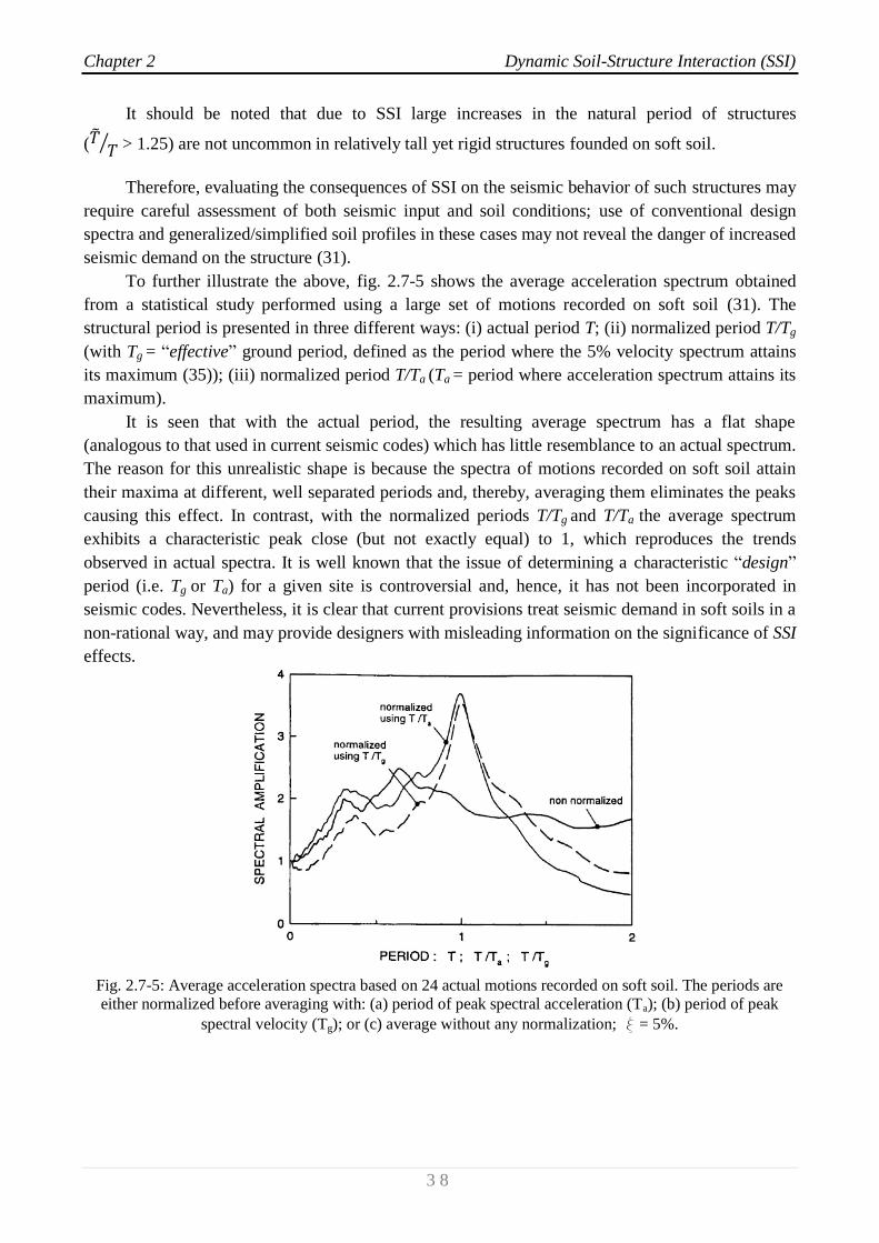
To further illustrate the above, fig. 2.7-5 shows the average acceleration spectrum obtained
from a statistical study performed using a large set of motions recorded on soft soil (31). The
structural period is presented in three different ways: (i) actual period T; (ii) normalized period T/Tg
(with Tg = “effective” ground period, defined as the period where the 5% velocity spectrum attains
its maximum (35)); (iii) normalized period T/Ta (Ta = period where acceleration spectrum attains its
maximum).
It is seen that with the actual period, the resulting average spectrum has a flat shape
(analogous to that used in current seismic codes) which has little resemblance to an actual spectrum.
The reason for this unrealistic shape is because the spectra of motions recorded on soft soil attain
their maxima at different, well separated periods and, thereby, averaging them eliminates the peaks
causing this effect. In contrast, with the normalized periods T/Tg and T/Ta the average spectrum
exhibits a characteristic peak close (but not exactly equal) to 1, which reproduces the trends
observed in actual spectra. It is well known that the issue of determining a characteristic “design”
period (i.e. Tg or Ta) for a given site is controversial and, hence, it has not been incorporated in
seismic codes. Nevertheless, it is clear that current provisions treat seismic demand in soft soils in a
non-rational way, and may provide designers with misleading information on the significance of SSI
effects.
Fig. 2.7-5: Average acceleration spectra based on 24 actual motions recorded on soft soil. The periods are
either normalized before averaging with: (a) period of peak spectral acceleration (Ta); (b) period of peak
spectral velocity (Tg); or (c) average without any normalization; x = 5%.
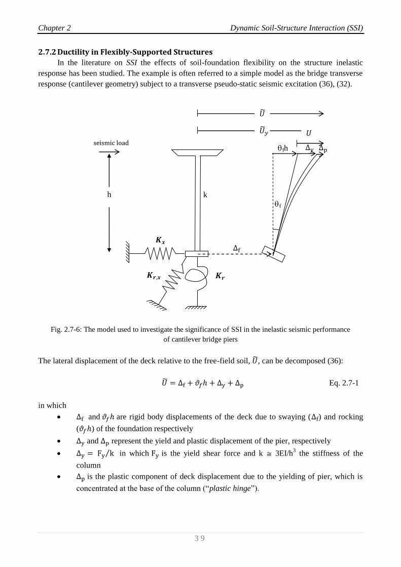
Chapter 2 Dynamic Soil-Structure Interaction (SSI)
3 9
fh
f
2.7.2 Ductility in Flexibly-Supported Structures
In the literature on SSI the effects of soil-foundation flexibility on the structure inelastic
response has been studied. The example is often referred to a simple model as the bridge transverse
response (cantilever geometry) subject to a transverse pseudo-static seismic excitation (36), (32).
Fig. 2.7-6: The model used to investigate the significance of SSI in the inelastic seismic performance
of cantilever bridge piers
The lateral displacement of the deck relative to the free-field soil, , can be decomposed (36):
Eq. 2.7-1
in which
and are rigid body displacements of the deck due to swaying ( ) and rocking
( ) of the foundation respectively
and represent the yield and plastic displacement of the pier, respectively
in which is the yield shear force and k 3EI/h3 the stiffness of the
column
is the plastic component of deck displacement due to the yielding of pier, which is
concentrated at the base of the column (“plastic hinge”).
h
k

Chapter 2 Dynamic Soil-Structure Interaction (SSI)
4 0
If the column were fixed at its base, eq. 2.7-1 would simplify to:
and dividing by would yield the displacement ductility factor of the column
Eq. 2.7-2
For the flexibly-supported system, the yielding displacement, , of the bridge is obtained by
setting to eq. 2.7-1:
The ratio
defines the so-called “global” or “system” displacement ductility factor of the
bridge-foundation system:
dividing by yields the dimensionless expression between and :
Eq. 2.7-3
in which
is a dimensionless coefficient expressing the foundation to structure displacement.
The next plot illustrates as a function of , for different values of the flexibility
coefficient c. For c = 0 (a structure fixed at its base), the values of the two factors coincide
( ). For c > 0, however, is always smaller than , decreasing monotonically with
increasing c. In fact, in the limiting case of c (an infinitely-flexible foundation or an
absolutely rigid structure), the “system” ductility is 1 regardless of the value of .
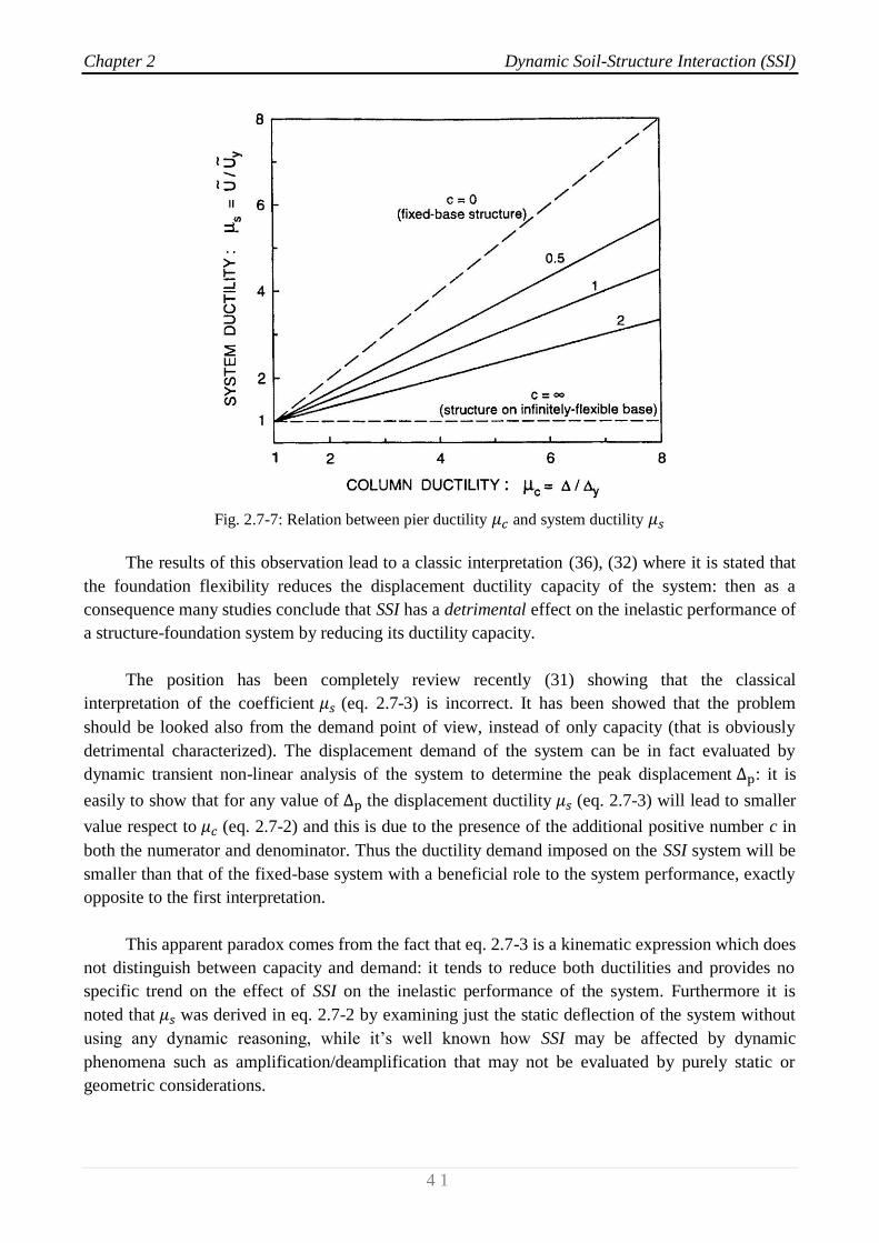
Chapter 2 Dynamic Soil-Structure Interaction (SSI)
4 1
Fig. 2.7-7: Relation between pier ductility and system ductility
The results of this observation lead to a classic interpretation (36), (32) where it is stated that
the foundation flexibility reduces the displacement ductility capacity of the system: then as a
consequence many studies conclude that SSI has a detrimental effect on the inelastic performance of
a structure-foundation system by reducing its ductility capacity.
The position has been completely review recently (31) showing that the classical
interpretation of the coefficient (eq. 2.7-3) is incorrect. It has been showed that the problem
should be looked also from the demand point of view, instead of only capacity (that is obviously
detrimental characterized). The displacement demand of the system can be in fact evaluated by
dynamic transient non-linear analysis of the system to determine the peak displacement : it is
easily to show that for any value of the displacement ductility (eq. 2.7-3) will lead to smaller
value respect to (eq. 2.7-2) and this is due to the presence of the additional positive number c in
both the numerator and denominator. Thus the ductility demand imposed on the SSI system will be
smaller than that of the fixed-base system with a beneficial role to the system performance, exactly
opposite to the first interpretation.
This apparent paradox comes from the fact that eq. 2.7-3 is a kinematic expression which does
not distinguish between capacity and demand: it tends to reduce both ductilities and provides no
specific trend on the effect of SSI on the inelastic performance of the system. Furthermore it is
noted that was derived in eq. 2.7-2 by examining just the static deflection of the system without
using any dynamic reasoning, while it’s well known how SSI may be affected by dynamic
phenomena such as amplification/deamplification that may not be evaluated by purely static or
geometric considerations.

Chapter 2 Dynamic Soil-Structure Interaction (SSI)
4 2
It is also criticized (31) the validity of as performance indicator, in fact this measure of
ductility of the system is affected by the presence of rigid body displacements due to the foundation
translation and rotation which are not associated with strain in the pier. This addition of rigid body
displacements in both the numerator and denominator of eq. 2.7-3 is the only reason for the
systematic drop in the ratio. This implies that the ductility ratio is not a measure of the distress of
the pier and as a limit example the hypothetical consideration of huge rigid body components both
at numerator and denominator will make equal to 1, even for a system that has failed.
On the evaluation of the foundation effects on structural inelastic performance a recent study
(37) confirmed the fact that only static considerations may lead to erroneous evaluations of
displacement ductility demand. It has been showed the importance of the dynamic behavior of the
foundation including the damping component that usually reduce the peak displacement and
ductility demands; in detail for columns ductility demand greater than 2.5 the effect of soil damping
induces a reduction of 70-80% respect to the ductility demand computed neglecting soil damping.
Chapter 3 The computer program SASSI2000
4 3
Chapter 3
The computer program SASSI2000
3.1 Introduction
The computer program SASSI2000 (a System for Analysis of Soil-Structure Interaction) was
developed at the University of California, Berkeley in 1991, by a research team directed by Prof. J.
Lysmer; the possibility of performing a 2D and 3D analysis as implemented in 1999 by Dr. Farhang
Ostadan.
Soil-Structure Interaction (SSI) problem is analyzed using a substructuring approach; in this
approach the linear problem is subdivided into a series of simpler sub-problems, each of them is
solved separately and the results are combined in the final step of the analysis to provide the
complete solution using the principle of superposition (38).
The basic methods of analysis adopted by SASSI2000 are formulated in the frequency domain,
using the complex response method and the finite element technique.
A detailed description of all the steps involved in a SASSI2000 analysis is beyond the
ambition of this chapter, for comprehensive understandings of the program see (38).

Chapter 3 The computer program SASSI2000
4 4
3.2 Substructuring methods in SASSI2000 analysis
Depending on how the interaction at the soil and structure interface degrees-of-freedom is
handled, two different methods are implemented in SASSI2000 to perform a substructuring
approach: the flexible volume method and the substructure subtraction method (39), (40).
Fig. 3.2-1 shows the three different seismic SSI sub-analysis required to be solved to obtain
the final solution, that is:
Site response analysis;
Impedance analysis;
Structural response analysis.
The site response problem solution as well as the analysis of the structural response problem
is required by both methods. The effort required for solving the impedance problem, however,
differs significantly among the two methods: because of the different substructuring technique (see
section 3.2.1 and 3.2.2), the subtraction method often requires a much smaller impedance analysis
than the flexible volume method (38).
3.2.1 The Flexible Volume Method (FVM)
The flexible volume substructuring method is based on the concept of partitioning the total
soil-structure system (see Fig. 3.2-2a) into three substructure systems (Figg. 3.2-2b,c,d).
Substructure I consists of the free-field site, substructure II consists of the excavated soil
volume, and substructure III consists of the structure where the excavated soil volume is replaced
by the foundation. Combining together the three substructures we obtain the original SSI system
(38).
The Flexible Volume Method presumes that the free-field site and the excavated soil volume
interact both at the boundary of the excavated soil volume and within its body, in addition to
interaction between the substructures at the boundary of the foundation of the structure.
The equation of motion for the undamped SSI substructures before mentioned can be written
in the following matrix form:
where and are the total mass and stiffness matrices respectively, is the vector of total
nodal point displacements and is the seismic excitation.
For the harmonic excitation at frequency , the seismic excitation and the displacement vector can
be written as:
tjeQ
tjeU
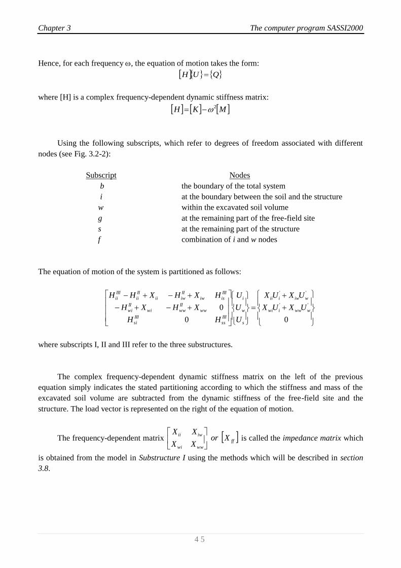
Chapter 3 The computer program SASSI2000
4 5
Hence, for each frequency , the equation of motion takes the form:
QUH
where [H] is a complex frequency-dependent dynamic stiffness matrix:
MKH 2
Using the following subscripts, which refer to degrees of freedom associated with different
nodes (see Fig. 3.2-2):
Subscript Nodes
b the boundary of the total system
i at the boundary between the soil and the structure
w within the excavated soil volume
g at the remaining part of the free-field site
s at the remaining part of the structure
f combination of i and w nodes
The equation of motion of the system is partitioned as follows:
00
0 ''
''
wwwiwi
wiwiii
s
w
i
III
ss
III
si
ww
II
wwwi
II
wi
III
isiw
II
iwii
II
ii
III
ii
UXUX
UXUX
U
U
U
HH
XHXH
HXHXHH
where subscripts I, II and III refer to the three substructures.
The complex frequency-dependent dynamic stiffness matrix on the left of the previous
equation simply indicates the stated partitioning according to which the stiffness and mass of the
excavated soil volume are subtracted from the dynamic stiffness of the free-field site and the
structure. The load vector is represented on the right of the equation of motion.
The frequency-dependent matrix ff
wwwi
iwiiXor
XX
XX
is called the impedance matrix which
is obtained from the model in Substructure I using the methods which will be described in section
3.8.

Chapter 3 The computer program SASSI2000
4 6
The vector
computed from the free-field motion for the interacting node
shown in Substructure I. The motion is a function of prescribed wave field in the free-field. The
methods for solving the site response problem for body and surface waves are described in section
3.4. Degrees of freedom associated with nodes i and w are considered interacting and included in
the impedance analysis and in the load vector.
Flexible Volume Substructure
Subtraction
Site Response
Analysis
Impedance
Analysis
Structural
Response
Analysis
STANDARD STANDARD
Fig. 3.2-1: Summary of substructuring methods adopted in SASSI2000
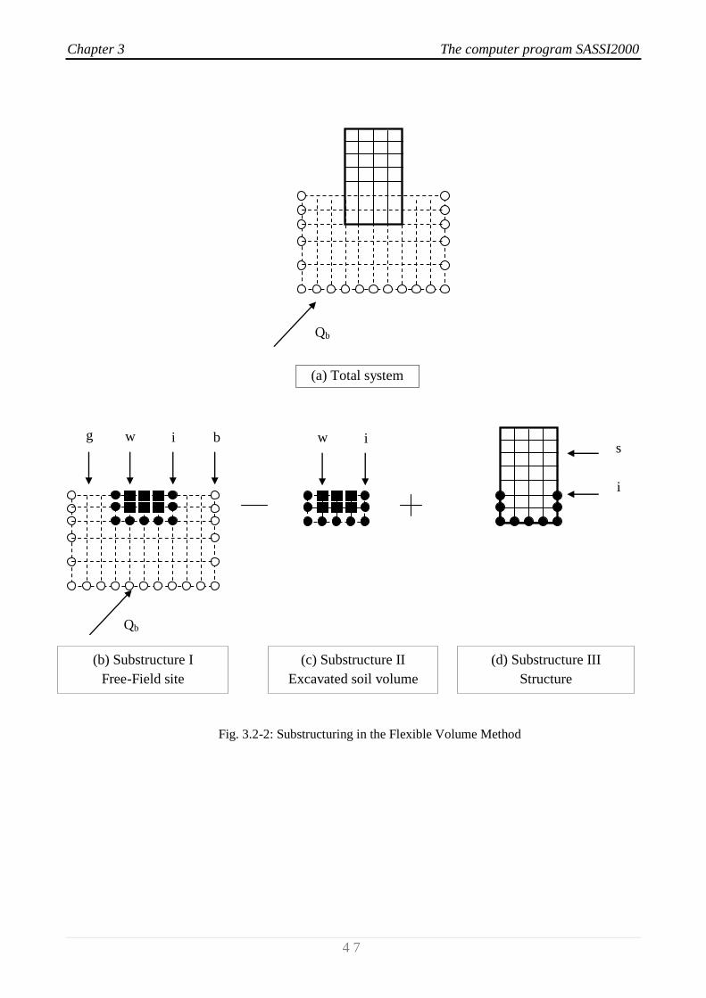
Chapter 3 The computer program SASSI2000
4 7
g w i w i b
(a) Total system
Fig. 3.2-2: Substructuring in the Flexible Volume Method
Qb
(b) Substructure I
Free-Field site
(c) Substructure II
Excavated soil volume
(d) Substructure III
Structure
Qb
s
i

Chapter 3 The computer program SASSI2000
4 8
3.2.2 The Substructure Subtraction Method (SM)
The substructure subtraction method is basically based on the same substructuring concept as
the flexible volume method. The subtraction method partitions the total soil-structure system as
shown in Fig. 3.2-3 into three substructure systems (Figg. 3.2-3b,c,d).
The subtraction method recognized that soil-structure interaction occurs only at the common
boundary of the substructures, that is, at the boundary of the foundation of the structure. This leads
to a smaller impedance analysis than the flexible volume method (38).
Following the same steps as in the flexible volume method, the equation of motion for the
subtraction method specializes as:
0
0
0
0
'
iii
s
w
i
III
ss
III
si
II
ww
II
wi
III
is
II
iwii
II
ii
III
ii UX
U
U
U
HH
HH
HHXHH
Compared with the equation of motion of the flexible volume method, this complex dynamic
stiffness is much simpler because only degrees of freedom associated with nodes i are considered
interacting. This also leads to an impedance analysis involving less number of degrees of freedom
and therefore a smaller impedance matrix or For the same reason only the free-field
motions at the degrees of freedom associated with nodes i, or
, computed from the site
response analysis are part of the load vector.
3.3 Computational steps
Based on the above formulations, a soil-structure interaction problem with seismic excitation
can be solved in the frequency domain according to the following five main steps (38):
1) Solve the site response problem. This step involves the determination of the free-field
displacement amplitude only for the interacting nodes of the free-field site. That is
in the flexible volume method or
in the subtraction method. For each frequency
of analysis, the free-field displacement vector is a function of the specified wave field
(body or surface waves and incident angle) and location of control point in the free-field
soil system.
2) Solve the impedance problem. This step involves the determination of the impedance
matrix which is a complex stiffness matrix corresponding to interacting nodes in
free-field soil medium. That is
wwwi
iwii
XX
XXin the flexible volume method and in
the subtraction method.
3) Form the load vector. This is obtained from the solutions of Step 1 and Step 2.
4) Form the complex stiffness matrix. The Finite Element Method is used to compute the
mass and stiffness matrix.
5) Solve the system of linear equations of motion.

Chapter 3 The computer program SASSI2000
4 9
b g w i i b
(a) Total system
Fig. 3.2-3: Substructuring in the Substructure Subtraction Method
Qb
(b) Substructure I
Free-Field site
(c) Substructure II
Excavated soil volume
(d) Substructure III
Structure
Qb
s
i

Chapter 3 The computer program SASSI2000
5 0
3.4 Site response analysis
For seismic excitation the free-field motion at interacting nodes, , must be computed.
Substructures (b) in Figg. 3.2-2 and 3.2-3 are used and the free- field motion is assumed to result
from a combination of coherent plane wave fields which may include P-, SV- and SH-body waves
or Rayleigh and Love surface waves (38).
The free-field site is assumed to consist of horizontal soil layers overlying either a rigid base
or an elastic halfspace using the technique to simulate the halfspace boundary condition at the base
as described in section 3.7.
A sketch of site response analyses is given in the following figure:
Fig. 3.4-1: Terminology used in site response analysis
The soil material properties are assumed to be viscoelastic; the complex modulus
representation is used to describe the properties of the soil layers. The equivalent linear method (41)
is used to approximate the nonlinear properties of the soil by equivalent linear properties, i.e.
equivalent linear shear modulus and damping ratio, which are compatible with the induced strain in
the soil medium.
To solve the site response problem for surface waves it is necessary to form and solve the
eigenvalue problem for the site model. Furthermore, the submatrices computed from the properties
of each layer to form the eigenequation are also used for body wave calculation.
A systematic description of the eigenvalue problem for site model is beyond the scope of this
section; a comprehensive presentation of these methods is available for example in (42).
In the next sections a brief introduction of the results of the eigenvalue problem is presented.
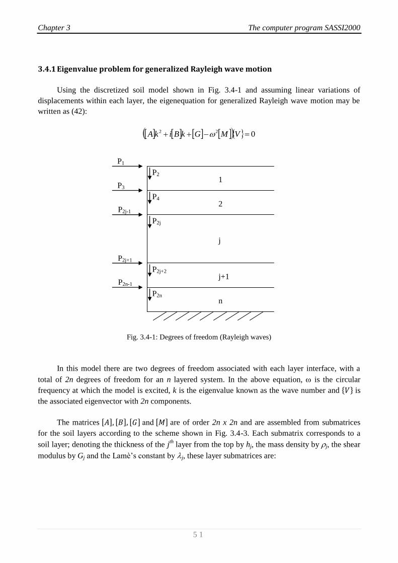
Chapter 3 The computer program SASSI2000
5 1
P1
P2
P4
P2j
P2j+2
P2n
1
2
j
j+1
n
P3
P2j-1
P2j+1
P2n-1
3.4.1 Eigenvalue problem for generalized Rayleigh wave motion
Using the discretized soil model shown in Fig. 3.4-1 and assuming linear variations of
displacements within each layer, the eigenequation for generalized Rayleigh wave motion may be
written as (42):
022 VMGkBikA
Fig. 3.4-1: Degrees of freedom (Rayleigh waves)
In this model there are two degrees of freedom associated with each layer interface, with a
total of 2n degrees of freedom for an n layered system. In the above equation, is the circular
frequency at which the model is excited, k is the eigenvalue known as the wave number and is
the associated eigenvector with 2n components.
The matrices and are of order 2n x 2n and are assembled from submatrices
for the soil layers according to the scheme shown in Fig. 3.4-3. Each submatrix corresponds to a
soil layer; denoting the thickness of the jth layer from the top by hj, the mass density by j, the shear
modulus by Gj and the Lamè’s constant by j, these layer submatrices are:
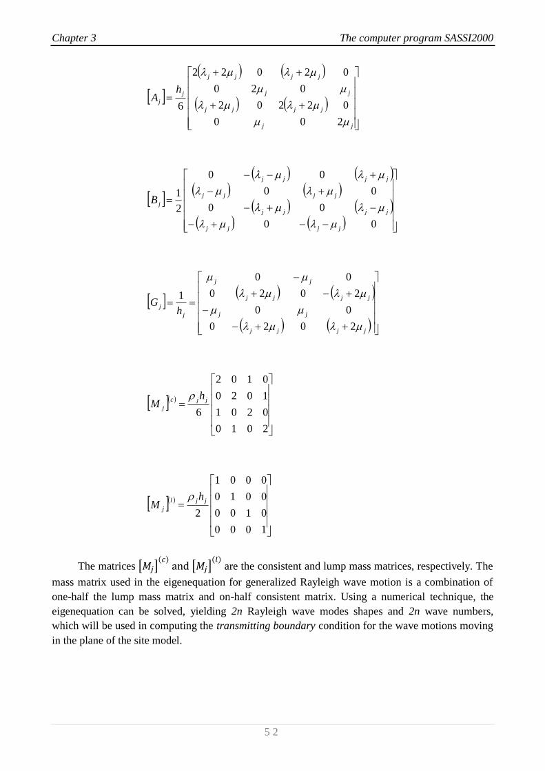
Chapter 3 The computer program SASSI2000
5 2
1000
0100
0010
0001
2
2010
0201
1020
0102
6
2020
00
2020
00
1
00
00
00
00
2
1
200
02202
020
02022
6
jjl
j
jjc
j
jjjj
jj
jjjj
jj
j
j
jjjj
jjjj
jjjj
jjjj
j
jj
jjjj
jj
jjjj
j
j
hM
hM
hG
B
hA
The matrices
are the consistent and lump mass matrices, respectively. The
mass matrix used in the eigenequation for generalized Rayleigh wave motion is a combination of
one-half the lump mass matrix and on-half consistent matrix. Using a numerical technique, the
eigenequation can be solved, yielding 2n Rayleigh wave modes shapes and 2n wave numbers,
which will be used in computing the transmitting boundary condition for the wave motions moving
in the plane of the site model.
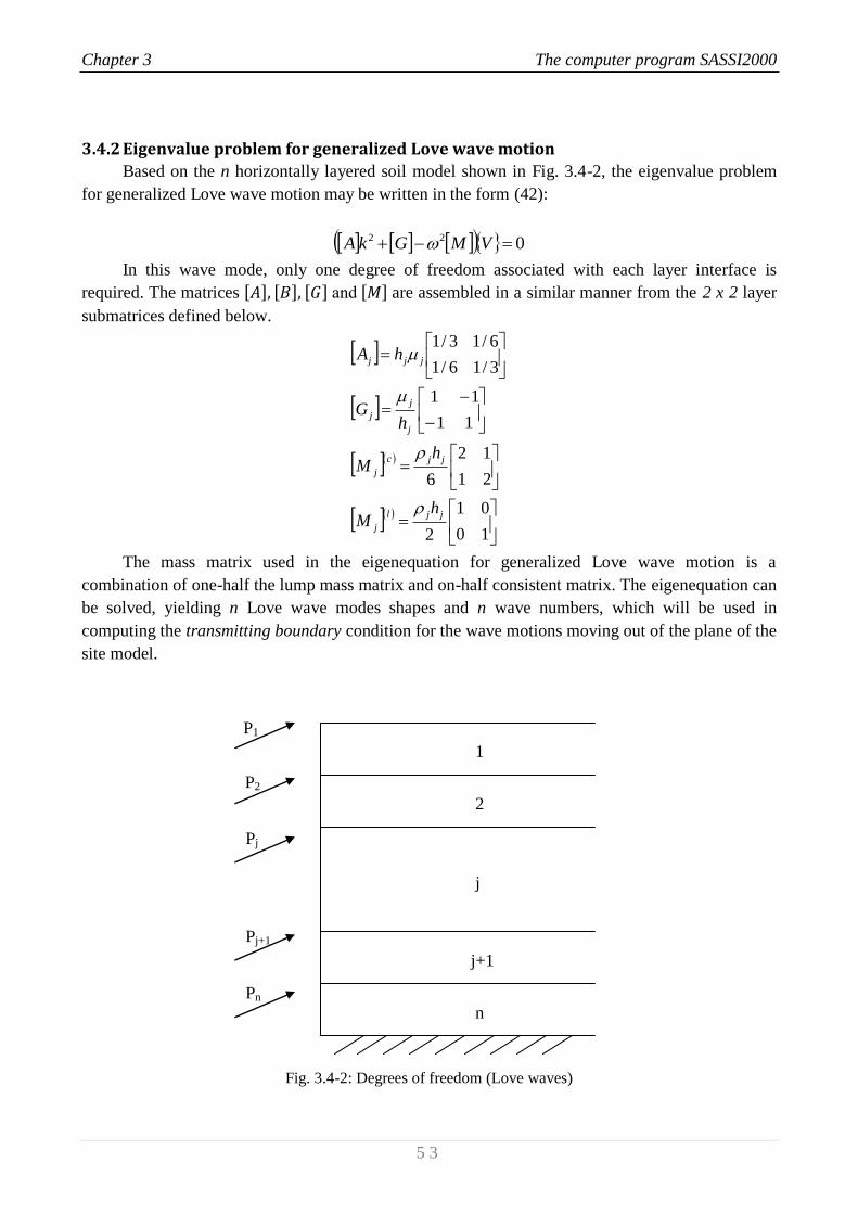
Chapter 3 The computer program SASSI2000
5 3
P1
1
2
j
j+1
n
P2
Pj
Pj+1
Pn
3.4.2 Eigenvalue problem for generalized Love wave motion
Based on the n horizontally layered soil model shown in Fig. 3.4-2, the eigenvalue problem
for generalized Love wave motion may be written in the form (42):
022 VMGkA
In this wave mode, only one degree of freedom associated with each layer interface is
required. The matrices and are assembled in a similar manner from the 2 x 2 layer
submatrices defined below.
10
01
2
21
12
6
11
11
3/16/1
6/13/1
jjl
j
jjc
j
j
j
j
jjj
hM
hM
hG
hA
The mass matrix used in the eigenequation for generalized Love wave motion is a
combination of one-half the lump mass matrix and on-half consistent matrix. The eigenequation can
be solved, yielding n Love wave modes shapes and n wave numbers, which will be used in
computing the transmitting boundary condition for the wave motions moving out of the plane of the
site model.
Fig. 3.4-2: Degrees of freedom (Love waves)
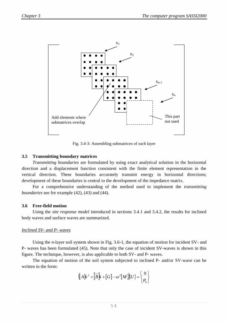
Chapter 3 The computer program SASSI2000
5 4
x1
x2
xn-1
xn
Fig. 3.4-3: Assembling submatrices of each layer
3.5 Transmitting boundary matrices
Transmitting boundaries are formulated by using exact analytical solution in the horizontal
direction and a displacement function consistent with the finite element representation in the
vertical direction. These boundaries accurately transmit energy in horizontal directions;
development of these boundaries is central to the development of the impedance matrix.
For a comprehensive understanding of the method used to implement the transmitting
boundaries see for example (42), (43) and (44).
3.6 Free-field motion
Using the site response model introduced in sections 3.4.1 and 3.4.2, the results for inclined
body waves and surface waves are summarized.
Inclined SV- and P- waves
Using the n-layer soil system shown in Fig. 3.6-1, the equation of motion for incident SV- and
P- waves has been formulated (45). Note that only the case of incident SV-waves is shown in this
figure. The technique, however, is also applicable to both SV- and P- waves.
The equation of motion of the soil system subjected to inclined P- and/or SV-wave can be
written in the form:
bP
UMGkBkA0
22
Add elements where
submatrices overlap
This part
not used
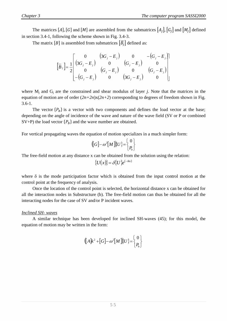
Chapter 3 The computer program SASSI2000
5 5
The matrices and are assembled from the submatrices and defined
in section 3.4-1, following the scheme shown in Fig. 3.4-3.
The matrix is assembled from submatrices defined as:
030
00
003
030
2
1
jjjj
jjjj
jjjj
jjjj
j
EGEG
EGEG
EGEG
EGEG
B
where Mj and Gj are the constrained and shear modulus of layer j. Note that the matrices in the
equation of motion are of order (2n+2n)x(2n+2) corresponding to degrees of freedom shown in Fig.
3.6-1.
The vector is a vector with two components and defines the load vector at the base;
depending on the angle of incidence of the wave and nature of the wave field (SV or P or combined
SV+P) the load vector and the wave number are obtained.
For vertical propagating waves the equation of motion specializes in a much simpler form:
bP
UMG0
2
The free-field motion at any distance x can be obtained from the solution using the relation:
ikxeUxU
where is the mode participation factor which is obtained from the input control motion at the
control point at the frequency of analysis.
Once the location of the control point is selected, the horizontal distance x can be obtained for
all the interaction nodes in Substructure (b). The free-field motion can thus be obtained for all the
interacting nodes for the case of SV and/or P incident waves.
Inclined SH- waves
A similar technique has been developed for inclined SH-waves (45); for this model, the
equation of motion may be written in the form:
bP
UMGkA0
22
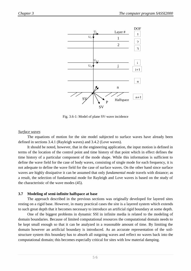
Chapter 3 The computer program SASSI2000
5 6
1
2
j
n
SV
SV
P
Layer # DOF
1
2
3
j
j+1
n
n+1
U1
U2
U2j-1
U2j
Fig. 3.6-1: Model of plane SV-wave incidence
Surface waves
The equations of motion for the site model subjected to surface waves have already been
defined in sections 3.4.1 (Rayleigh waves) and 3.4.2 (Love waves).
It should be noted, however, that in the engineering application, the input motion is defined in
terms of the location of the control point and time history of that point which in effect defines the
time history of a particular component of the mode shape. While this information is sufficient to
define the wave field for the case of body waves, consisting of single mode for each frequency, it is
not adequate to define the wave field for the case of surface waves. On the other hand since surface
waves are highly dissipative it can be assumed that only fundamental mode travels with distance; as
a result, the selection of fundamental mode for Rayleigh and Love waves is based on the study of
the characteristic of the wave modes (45).
3.7 Modeling of semi-infinite halfspace at base
The approach described in the previous sections was originally developed for layered sites
resting on a rigid base. However, in many practical cases the site is a layered system which extends
to such great depth that it becomes necessary to introduce an artificial rigid boundary at some depth.
One of the biggest problems in dynamic SSI in infinite media is related to the modeling of
domain boundaries. Because of limited computational resources the computational domain needs to
be kept small enough so that it can be analyzed in a reasonable amount of time. By limiting the
domain however an artificial boundary is introduced. As an accurate representation of the soil-
structure system this boundary has to absorb all outgoing waves and reflect no waves back into the
computational domain; this becomes especially critical for sites with low material damping.
Halfspace
Chapter 3 The computer program SASSI2000
5 7
To remedy this problem, two techniques are implemented in SASSI2000 to simulate the semi-
infinite halfspace at the soil layer base, that is:
The variable depth method;
Absorbing Lysmer Boundaries at base.
The variable depth method consists in adding n extra layers to the base of the top soil layers;
in order to introduce a minimal error in representing the halfspace, the total depth H of the added
layers must vary with the frequency of analysis, and is set to:
where f is the frequency of analysis in Hz (38).
The site model may be further improved by replacing the rigid boundary with a viscous
boundary, which consists of two dashpots per unit area of the boundary (46).
The dashpots have the damping coefficients:
Vertical dashpot: Cp = Vp
Horizontal dashpot: Cs = Vs
where is the mass density and Vp and Vs are the P- and S- wave velocities of the halfspace below
the boundary of the model.
The inclusion of dashpots in the site model also greatly improves the accuracy of the
impedance calculations.
3.8 Impedance analysis
The solution of the equation of motion of the SSI system based on the flexible volume and the
substructure subtraction methods used by SASSI2000 include the computation of the impedance
matrix [Xff] as shown in section 3.2.1 and 3.2.2. In the former method the impedance matrix needs
to be computed for all the interacting nodes, in the latter only for the exterior boundary nodes (38).
The computation of the impedance matrix is achieved by inverting the dynamic flexibility
(compliance) matrix (i.e. [Xff] = [Fff]-1
) for each frequency of analysis. By definition of the
compliance matrix, the components of the ith
column of the matrix are the dynamic displacements
of the interacting degrees of freedom caused by harmonic force unit amplitude acting at the ith
degree of freedom. Thus, the problem of determining the compliance matrix for 2D problems is that
of finding the harmonic response displacements of all the nodes subjected to harmonic line load, as
shown in Fig. 3.8-1, placed successively at one column of nodes shown as heavy dots. Once this
problem has been solved, solution corresponding to other nodes can be obtained simply by a shift of
the horizontal coordinates.
The basic solution is obtained using a model which consists of a single column of plane-strain
rectangular elements. The existence of the semi-infinite layered region is simulated by applying the
consistent transmitting boundary impedances as seen in section 3.5.

Chapter 3 The computer program SASSI2000
5 8
Embedment
Transmitting
boundaries
The problem of evaluating the dynamic flexibility matrix for a 3D-case can be easily
generalized from the 2D-case, considering the axisymmetry of the model.
Fig. 3.8-1: Plane-Strain model for impedance analysis
Rigid base
x Basement node
Loaded node

Chapter 3 The computer program SASSI2000
5 9
3.9 Computer program organization
The computer program SASSI2000 (47) is written in the Fortran IV language; the analysis
steps of the program are organized in different modules. Fig. 3.9-1 shows the layout of the program.
A brief description of the function of each module and its interaction with other modules are
presented in the following (38):
HOUSE
In this module the mass and stiffness matrices of all the elements (i.e. structure and excavated
soil) used in the model are computed and stored in Tape 4. These properties are frequency
independent and the computation is performed only once.
MOTOR
This module forms the load vector. The loads may correspond to impact forces, rotating
machinery or simple unit forces to be used to determine the impedance of a foundation. It is
possible to allow for loads acting out of phase. The results are stored on Tape 9.
SITE
This module solves the site response problem. The control point and wave composition of the
control motion are defined. The information needed to compute vector is computed at this
stage and is saved in Tape 1. The program also stores information required for the transmitting
boundary calculation on Tape 2. The actual time history of the control motion is not required in this
module.
POINT
This module consists of two submodules, namely POINT2 and POINT3, for 2D and 3D
problems respectively. The results, which provide the information required to form the flexibility
matrix, are saved on Tape 3. Tape 2 created by program SITE is used as input.
ANALYS
This module is the heart of program SASSI2000. It drives the three subprograms MATRIX (it
forms the impedance matrix [Xff()] and triangularizes the coefficient matrix), LOAD (it computes
the load vector for each frequency) and SOLVE (it computes the transfer functions from the control
motion to the final motion) and thereby controls the restart modes of the program.
Interpolation of the transfer functions in the frequency domain and further output
requirements are handled by the following subprograms:
MOTION
This program is a post-processor. It reads the transfer function and computes the final
response at specified nodes selected by the user. Acceleration, velocity and displacement of the
response in terms of time history, peak value or the response spectrum may be requested.

Chapter 3 The computer program SASSI2000
6 0
STRESS
This module computes requested stress, strain and forces time histories and peak values in
structural members.
COMBINE
If after interpolation it is found that some additional frequencies need to be included, this
program combines the previous results with the added frequencies.
3.10 Capabilities and limitations
The current version of SASSI2000 has the following capabilities and limitations:
Soil and Structure Idealization
1. The site consists of semi-infinite elastic or viscoelastic horizontal layers on a rigid base or
a semi-infinite elastic or viscoelastic halfspace.
2. The structure is idealized by standard 2D or 3D finite elements connected at nodal points.
3. Each nodal point on the structure may have up to six displacement degrees of freedom.
The user has the option to delete one or more of the degrees of freedom thereby reducing
the size of the problem accordingly.
4. The excavated soil zone is idealized by standard plane strain or 3D solid elements. The
finite element models of the structure and excavated soil have common nodes at the
boundary.
5. Depending on the method selected for impedance analysis, the interaction between the
foundation and the structure occurs at all basement nodes, including those in the basement
volume or occurs only at the common boundary nodes.
6. All the interaction nodes lie on the soil layer interfaces with translational degree-of-
freedom. Rotations from the structure are transferred by translation by connecting at
several interacting nodes.
7. The mass matrix is assumed to be 50% lumped and 50% consistent except for the
structural beam elements and plate elements where consistent mass matrix and lump mass
matrix are used, respectively.
8. Material damping is introduced by the use of complex moduli, which leads to effective
damping ratios which are frequency-independent and may vary from element to element.
Dynamic Loadings
1. The seismic environment may consist of an arbitrary 3D superposition of inclined body
waves and surface waves.
2. Earthquake excitation is defined by a time history of acceleration called control motion.
The control motion is assigned to one of the three global directions at the control point
which lies on a soil layer interface.
3. In addition to seismic loads, it is possible to introduce external forces or moments such as
impact loads, wave forces, or loads from rotating machinery acting directly on the
structure. It is possible to assign different maximum amplitudes and arrival times to each
dynamic load applied at a nodal point.

Chapter 3 The computer program SASSI2000
6 1
4. Transient input time histories such as earthquake record or impact loads are handled by
the Fast Fourier Transform technique. Therefore, the time histories must be specified at
equal time intervals.
Nonlinear Analysis
1. The analytical method used in the SASSI2000 program is restricted to linear analysis.
However, approximate nonlinear analysis can be performed by an iterative scheme called
Equivalent Linear Method.
2. Primary nonlinear effects in the free-field and secondary nonlinear effects in a limited
region near the structure can be considered.
Fig. 3.9-1: Layout of computer program SASSI2000
Chapter 4 Generalized Single Degree of Freedom System
6 2
Chapter 4
Generalized Single Degree of Freedom Systems
4.1 Introduction
The analysis of a complex system can be approached by its simplification as Single Degree of
Freedom (SDOF) system; such system is called generalized SDOF system.
The analysis provides exact results for an assemblage of rigid bodies supported such that it
can deflect in only one shape, but only approximate results for systems with distributed mass and
flexibility. In the latter case, the approximate natural frequency is shown to depend on the assumed
deflected shape (48).
In both categories, the structure is forced to behave like a SDOF system by the fact that
displacements of only a single form or shape are permitted; the assumed deflection can be related to
a single generalized displacement z(t) through a shape function (x) that approximates the
fundamental vibration mode and can be expressed as:
The equation of motion for a generalized SDOF system is of the form:
where are defined as the generalized mass, generalized damping, generalized
stiffness and generalized force of the system: these generalized properties are associated with the
generalized displacement z(t) selected (49).
Since the aim of the present research is the evaluation of the response of generalized SDOF
systems representing different configurations of shear buildings, the following part of the chapter
will be focused on the estimate of generalized properties of lumped-mass systems.

Chapter 4 Generalized Single Degree of Freedom System
6 3
4.2 Lumped-mass system: shear building
As an illustration of approximating a system having several degrees of freedom by a
generalized SDOF system, consider the frame shown in Fig. 4.2-1 and earthquake excitation. The
mass of this N-storey frame is lumped at the floor levels with mj denoting the mass at the jth
floor.
This system has N degrees of freedom: u1, u2, …, uN. First the equation of motion for this system
without damping is formulated; damping is usually defined by a damping ratio estimated from
experimental data for similar structures. Then the equation of motion is solved to determine the
peak response (displacements and internal forces) of the structure to earthquake ground motion
(48).
Fig. 4.2.1: Lumped-mass system - Shear building
4.3 Assumed shape vector
We assume that the floor displacements relative to the ground can be expressed as (48):
which in vector form is
where is an assumed shape vector that defines the deflected shape. The total displacement
of the jth
floor is
m2
ug(t)
hj
mN
mj
m1
N
j
2
1
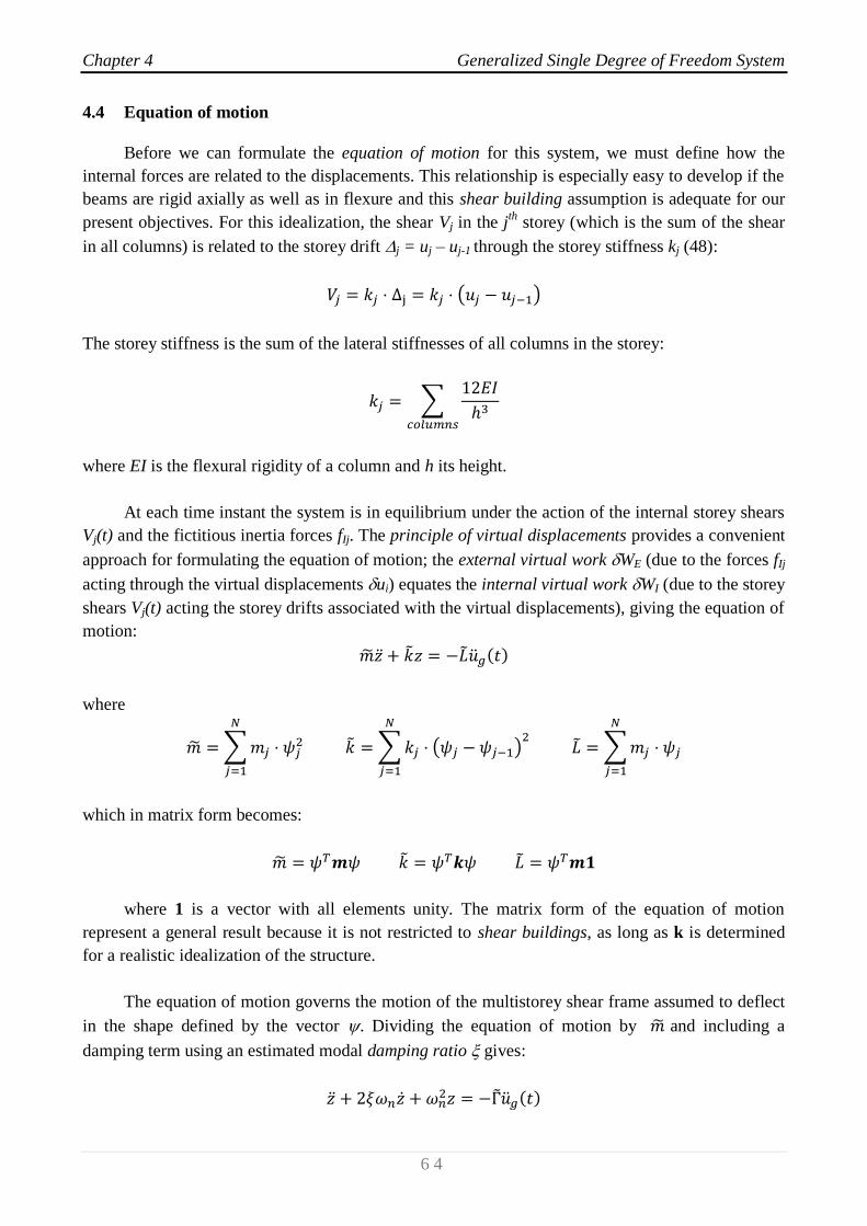
Chapter 4 Generalized Single Degree of Freedom System
6 4
4.4 Equation of motion
Before we can formulate the equation of motion for this system, we must define how the
internal forces are related to the displacements. This relationship is especially easy to develop if the
beams are rigid axially as well as in flexure and this shear building assumption is adequate for our
present objectives. For this idealization, the shear Vj in the jth
storey (which is the sum of the shear
in all columns) is related to the storey drift j = uj – uj-1 through the storey stiffness kj (48):
The storey stiffness is the sum of the lateral stiffnesses of all columns in the storey:
where EI is the flexural rigidity of a column and h its height.
At each time instant the system is in equilibrium under the action of the internal storey shears
Vj(t) and the fictitious inertia forces fIj. The principle of virtual displacements provides a convenient
approach for formulating the equation of motion; the external virtual work WE (due to the forces fIj
acting through the virtual displacements ui) equates the internal virtual work WI (due to the storey
shears Vj(t) acting the storey drifts associated with the virtual displacements), giving the equation of
motion:
where
which in matrix form becomes:
where 1 is a vector with all elements unity. The matrix form of the equation of motion
represent a general result because it is not restricted to shear buildings, as long as k is determined
for a realistic idealization of the structure.
The equation of motion governs the motion of the multistorey shear frame assumed to deflect
in the shape defined by the vector . Dividing the equation of motion by and including a
damping term using an estimated modal damping ratio gives:

Chapter 4 Generalized Single Degree of Freedom System
6 5
where
and .
The approximate generalized natural frequency obtained from an assumed shape function is
never smaller than the exact value of the fundamental natural frequency of the actual system; such
interesting characteristic is particularly appealing because in case the exact value of the natural
frequency is unknown, as would be the case for complex systems, we could say that its best
estimate is represented by the smallest of the generalized natural frequency value among all the
other estimates.
4.5 Response analysis
The next step is to compute the internal forces (i.e. bending moments, shears and axial forces)
and stresses in the building associated with the displacements . Such forces are computed by
static analysis of the structure at each instant in time; this static analysis is computed introducing the
equivalent static force fS, i.e. slowly applying at any instant of time t the external force fS that will
produce the deformation determined by dynamic analysis (48). Thus .
For a generalized SDOF system the equivalent static force can be expressed as:
4.6 Peak earthquake response
If the response spectrum for a given ground motion component is available, the peak value of
deformation or of an internal force in any linear generalized SDOF system can be determined
readily. Corresponding to the generalized natural vibration period and damping ratio of the
system, the values of the deformation D, pseudo-velocity V and pseudo-acceleration I response
spectra are read from the spectrum. Now all response quantities of interest can be expressed in
terms of D, V or A and the mass or stiffness properties of the system (48).
Suppose that it is desired to determine the peak response of the frame to earthquake excitation
characterized by a design spectrum. The peak value of z(t) is given by:
The floor displacements relative to the ground are given by:
The equivalent static forces associated with these floor displacements are given by:

Chapter 4 Generalized Single Degree of Freedom System
6 6
Finally, the shear Vb0 and overturning moment Mb0 at the base are:
where
Once Vb0 and Mb0 have been estimated, we can simply derive the height h of the equivalent
oscillator by diving the overturning moment by the shear at the base:
Fig. 4.6.1: Base shear and moment
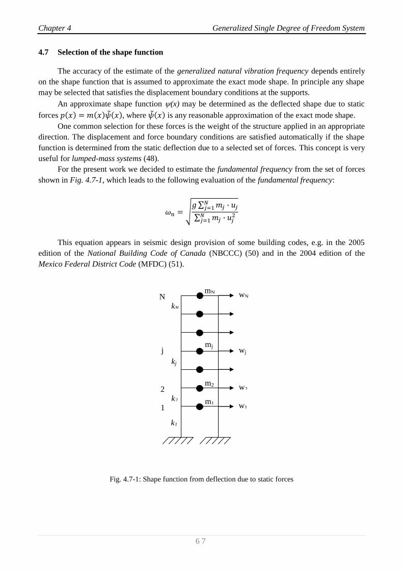
Chapter 4 Generalized Single Degree of Freedom System
6 7
j
k2
kj
kN
k1
4.7 Selection of the shape function
The accuracy of the estimate of the generalized natural vibration frequency depends entirely
on the shape function that is assumed to approximate the exact mode shape. In principle any shape
may be selected that satisfies the displacement boundary conditions at the supports.
An approximate shape function (x) may be determined as the deflected shape due to static
forces , where is any reasonable approximation of the exact mode shape.
One common selection for these forces is the weight of the structure applied in an appropriate
direction. The displacement and force boundary conditions are satisfied automatically if the shape
function is determined from the static deflection due to a selected set of forces. This concept is very
useful for lumped-mass systems (48).
For the present work we decided to estimate the fundamental frequency from the set of forces
shown in Fig. 4.7-1, which leads to the following evaluation of the fundamental frequency:
This equation appears in seismic design provision of some building codes, e.g. in the 2005
edition of the National Building Code of Canada (NBCCC) (50) and in the 2004 edition of the
Mexico Federal District Code (MFDC) (51).
Fig. 4.7-1: Shape function from deflection due to static forces
m2
mN
mj
m1 w1
w2
wj
wN N
2
1
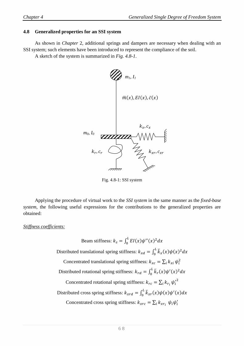
Chapter 4 Generalized Single Degree of Freedom System
6 8
4.8 Generalized properties for an SSI system
As shown in Chapter 2, additional springs and dampers are necessary when dealing with an
SSI system; such elements have been introduced to represent the compliance of the soil.
A sketch of the system is summarized in Fig. 4.8-1.
Fig. 4.8-1: SSI system
Applying the procedure of virtual work to the SSI system in the same manner as the fixed-base
system, the following useful expressions for the contributions to the generalized properties are
obtained:
Stiffness coefficients:
Beam stiffness:
Distributed translational spring stiffness:
Concentrated translational spring stiffness:
Distributed rotational spring stiffness:
Concentrated rotational spring stiffness:
Distributed cross spring stiffness:
Concentrated cross spring stiffness:
m1, I1
m0, I0
Chapter 4 Generalized Single Degree of Freedom System
6 9
Damping:
Beam damping:
Distributed translational damping:
Concentrated translational damping:
Distributed rotational damping:
Concentrated rotational damping:
Distributed cross spring damping:
Concentrated cross spring damping:
Mass coefficients:
Distributed mass:
Concentrated mass:
Distributed moment of inertia:
Concentrated moment of inertia:
External loads:
Distributed force:
Concentrated force:
Distributed moment:
Concentrated moment:
For the system shown in Fig. 4.8.1 the generalized natural frequency and damping are computed as:
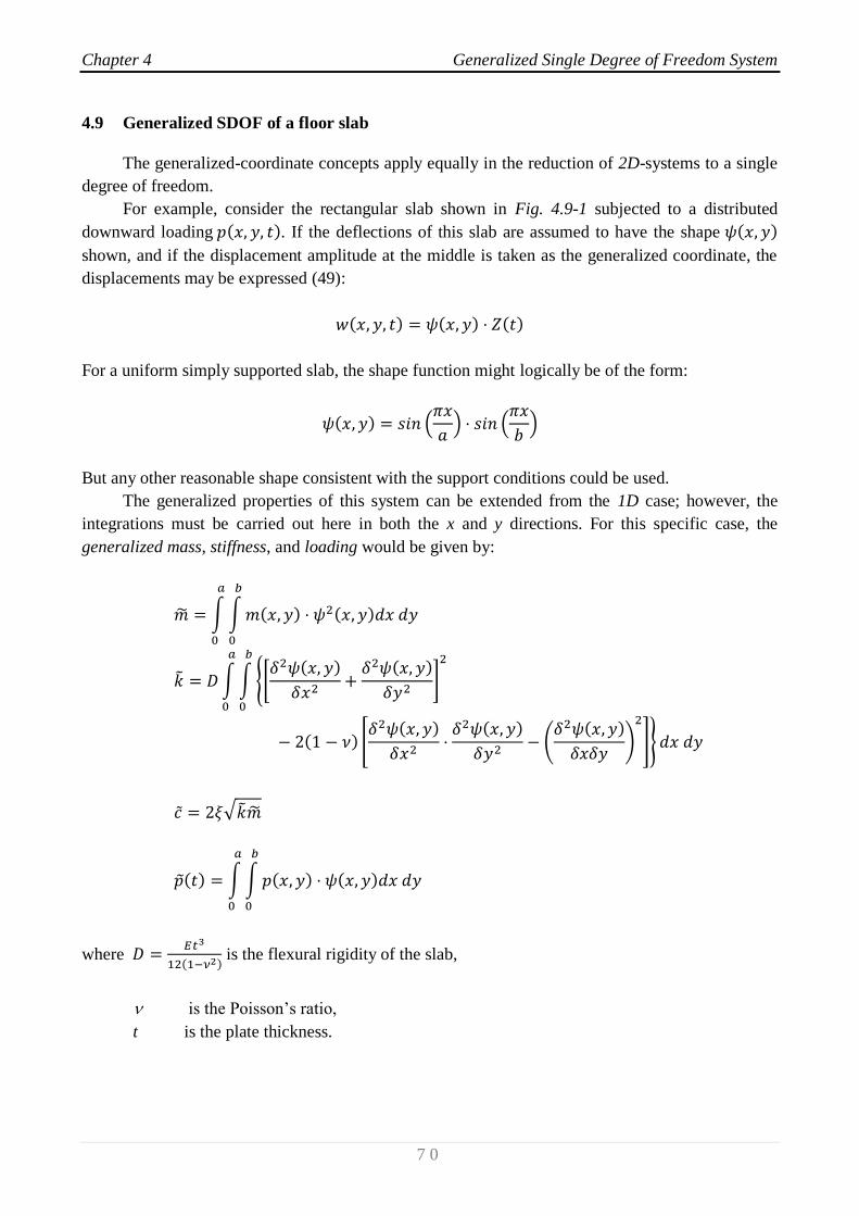
Chapter 4 Generalized Single Degree of Freedom System
7 0
4.9 Generalized SDOF of a floor slab
The generalized-coordinate concepts apply equally in the reduction of 2D-systems to a single
degree of freedom.
For example, consider the rectangular slab shown in Fig. 4.9-1 subjected to a distributed
downward loading . If the deflections of this slab are assumed to have the shape
shown, and if the displacement amplitude at the middle is taken as the generalized coordinate, the
displacements may be expressed (49):
For a uniform simply supported slab, the shape function might logically be of the form:
But any other reasonable shape consistent with the support conditions could be used.
The generalized properties of this system can be extended from the 1D case; however, the
integrations must be carried out here in both the x and y directions. For this specific case, the
generalized mass, stiffness, and loading would be given by:
where
is the flexural rigidity of the slab,
is the Poisson’s ratio,
t is the plate thickness.
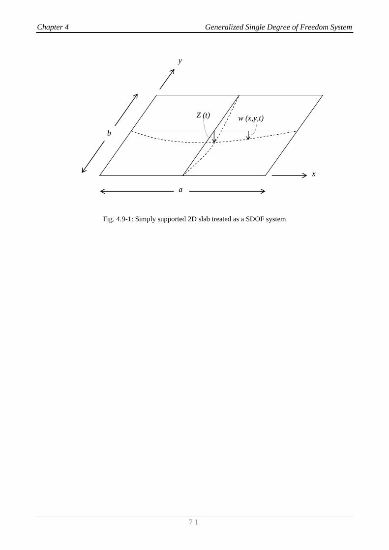
Chapter 4 Generalized Single Degree of Freedom System
7 1
Fig. 4.9-1: Simply supported 2D slab treated as a SDOF system
x
y
b
a
Z (t) w (x,y,t)
Chapter 5 Performed analysis and results
7 2
Chapter 5
Performed analyses and results
5.1 Introduction
This doctoral work focuses on the hazard and structural vulnerability assessment of ordinary
reinforced-concrete structures with respect to seismic risk and attempts to make two main
contributions with regards to structures founded on superficial foundation.
First, a systematic application of complete SSI analyses to different types of buildings (up to
twenty storeys), has been performed; the compliance of the ground has been evaluated by means of
the computer program SASSI2000 (Lysmer et al., 1999). Concrete shear-type structures have been
modeled as generalized Single Degree Of Freedom (SDOF) systems using the principle of virtual
displacements, while different soil conditions (consistent with the EC8-I), foundation depths and
seismic excitations are taken into account. The modified characteristics of the buildings, in terms of
modified damping and period, have been estimated, comparing a classical solution (Wolf, 1985) and
a recent exact procedure (Mylonakis, 2006); results are presented in form of ready-to-use non-
dimensional charts.
The second main contribution of this work is a sort of “pre-normative" study concerning SSI
assessment, which could be useful to enhance the codes, as a measure of risk mitigation; SSI effect
has been evaluated in terms of maximum accelerations at the top of the buildings and a systematic
comparison with the fixed-base solutions has been performed. The final goal is the set-up of
simplified charts and tables that can be easily used by practitioners who want to face the task of SSI
in an immediate and simplified manner, without performing an expensive and time-consuming
analysis.
Chapter 5 Performed analysis and results
7 3
5.2 Seismic Inputs
The assessment of the structural response via dynamic analysis requires some characterization
of the seismic input which should reflect the hazard as well as the near-surface geology at the site.
Generally, the signals that can be used for the seismic structural analysis are of three types: (a)
artificial waveforms; (b) simulated accelerograms; and (c) natural records (52).
Spectrum-compatible signals of type (a) are obtained, for example, generating a power
spectral density function from the code response spectrum, and deriving signals compatible to that.
However, this approach may lead to accelerograms not reflecting the real phasing of seismic waves
and cycles of motion, and therefore energy. For such reasons these kind of seismic inputs have not
been considered in this work
Simulation records (b) are obtained via modeling of the seismological source and may
account for path and site effects. These methods range from stochastic simulation of point or finite
sources to dynamic models of rupture.
Synthetics may be the only way to obtain appropriate records for rare scenarios, such as large
magnitude events “close” to the site and give the benefit that one can produce from them large
samples of nominally similar events. They often require setting of some rupture parameters, such as
the rise-time, which are hard to determine.
Finally, of type (c) are ground-motion records from real events. The availability of on-line,
user-friendly, databases of strong-motion recordings, and the rapid development of digital seismic
networks worldwide, has increased the accessibility to recorded accelerograms.
However, due to the large variability in records representing a scenario, a number of points
arise regarding the criteria for appropriate selection and manipulation of such records. In particular,
an issue regarding the use of real recordings, whose spectra are generally non-smoothed, is the
selection of a set compatible with a code-specified spectrum.
It is beyond the scope of this work to describe the developed methods (either in the
frequency-domain and time-domain) to manipulate real records to match a target spectral shape,
although it is worthy to say that these methods produce records perfectly compatible with code’s
prescriptions and have the additional advantage of reducing the dispersion in the response, and
hence the required sample size.
As previously mentioned, the code-based prescriptions for records often require compatibility
with a smooth design acceleration spectrum together with few other minor requirements. Eurocode
8 (EC8-I), in particular, allows employment of all three kinds of accelerograms listed above as an
input for seismic structural analysis. The EC8 prescriptions ask for matching of the average spectral
ordinates of the chosen record set to the target code-based spectral shape. The set has to consist of
at least seven recordings (each of which includes both horizontal components of a recorded motion
if spatial analysis is concerned) to consider the mean of the response. Otherwise, if the size of the
set is from three to six, the maximum response to the records within the sets needs to be considered.
Little, if any, prescriptions are given about other features of the signal. Therefore, the code
requirements seem to have been developed having spectrum-compatible records in mind. On the
other hand, real accelerograms are becoming the most attractive option to get unbiased estimations
of the seismic demand (53).

Chapter 5 Performed analysis and results
7 4
5.2.1 Spectrum-matching earthquakes
Recent Codes (EC8-I) require to define a design (reference) spectrum whose ordinates have a
small probability of exceedance. Secondly, a scenario event or design earthquake has to be defined
referring to the local seismicity. Then, in the case of nonlinear dynamic analysis, codes basically
require a certain number of records to be chosen consistently with the design earthquake and the
code spectrum in a broad range of periods. Finally, the performance of the structure is assessed
verifying whether the maximum or average response of the structure to the records exceeds the
seismic capacity (54).
Among all the possible options to define the seismic input for structural analysis, natural
recordings are emerging as the most attractive. Easily accessible waveform databases are available
and evidence shows that only a relatively limited number of criteria have to be considered in
selection and scaling to get an unbiased estimation of seismic demand. Like many codes worldwide,
Eurocode 8 (EC8-I) allows the use of real ground-motion records for the seismic assessment of
structures (53).
Another good reason for their use is simply the scarcity of recorded ground motion for many
regions in the world.
The main condition to be satisfied by the chosen set is that the average elastic spectrum does
not underestimate the code spectrum, with a 10% tolerance, in a broad range of periods depending
on the structure's dynamic properties. The EC8-I prescriptions seem to favor the use of spectrum-
matching records, obtained either by simulation or manipulation of real records.
Once the reference spectrum has been defined, the set of accelerograms, regardless if they are
natural, artificial, or simulated, should match the following criteria:
a) a minimum of 3 accelerograms should be used;
b) the mean of the zero period spectral response acceleration values (calculated from
the individual time histories) should not be smaller than the value of ag S for the site
in question;
c) in the range of periods between 0,2T1 and 2T1, where T1 is the fundamental period of
the structure in the direction where the accelerogram will be applied; no value of the
mean 5% damping elastic spectrum, calculated from all time histories, should be less
than 90% of the corresponding value of the 5% damping elastic response spectrum.
For ordinary structures it is assumed herein that a group of records is only made up of the two
horizontal components of a recorded signal.
The code allows the consideration of the mean effects on the structure, rather than the
maximum, if at least seven nonlinear time-histories analyses are performed.

Chapter 5 Performed analysis and results
7 5
5.2.2 Near-Fault registered earthquakes
A site located close to the source of a seismic event may be in a geometrical configuration, in
respect to the propagating rupture, which may favor the constructive interference of waves
(synchronism of phases causing building up of energy) traveling to it, which may result in a large
velocity pulse, that clearly distinguish them from typical far-field ground motions
This situation, for dip-slip faults, requires the rupture going toward the site and the alignment
of the latter with the dip of the fault, whereas for strike-slip faults the site must be aligned with the
strike; if these conditions are met the ground-motion at the site may show forward directivity effects
(33).
This observation, along with its engineering significance, was first made with respect to the
Station 2 (C02) record generated by the 1966 Parkfield, California, earthquake at a distance of only
80m from the fault break. The physical interpretation and numerical modeling of the C02 record is
considered to be the starting point for modern quantitative analysis of strong ground motion
observations (55).
The damage that the Olive View Hospital sustained during the 1971 San Fernando,
California, earthquake was attributed to the effect of the near-fault ground motions on flexible
structures (56); it was the first time that earthquake engineers linked the structural damage caused
by an earthquake to the impulsive character of the near-source ground motions. However, it was
only after the 1994 Northridge, California and the 1995 Kobe, Japan earthquakes that the majority
of engineers recognized the severe implications and the destructive potential of the near-fault
ground motion pulses on the urban infrastructure when the causative fault is in the immediate
vicinity of large metropolitan areas.
In general, forward directivity and permanent translation are the two main causes for the
velocity pulses observed in near-field regions.
Forward directivity occurs when the fault rupture propagates toward a site with a rupture
velocity approximately equal to the shear-wave velocity. In this case, most of the elastic energy
arrives coherently in a single, intense, relatively long-period pulse at the beginning of the record,
representing the cumulative effect of almost all the seismic radiation from the fault. The
phenomenon is even more pronounced when the direction of slip on the fault plane points toward
the site as well.
On the other hand, permanent translation at a site is a consequence of permanent fault
displacement due to an earthquake; it appears in the form of step displacement and one-sided
velocity pulse in the strike-parallel direction for strike-slip faults (e.g., stations YPT and SKR from the
1999 Izmit, Turkey, earthquake) or in the strike-normal direction for dip-slips faults.
It can be stated that rupture directivity produces a narrowband velocity pulse, the period of
which increases with earthquake magnitude (55).
In figure 5.2-1 the velocity pulses of selected near-fault earthquake are illustrated in visually
informative manner.
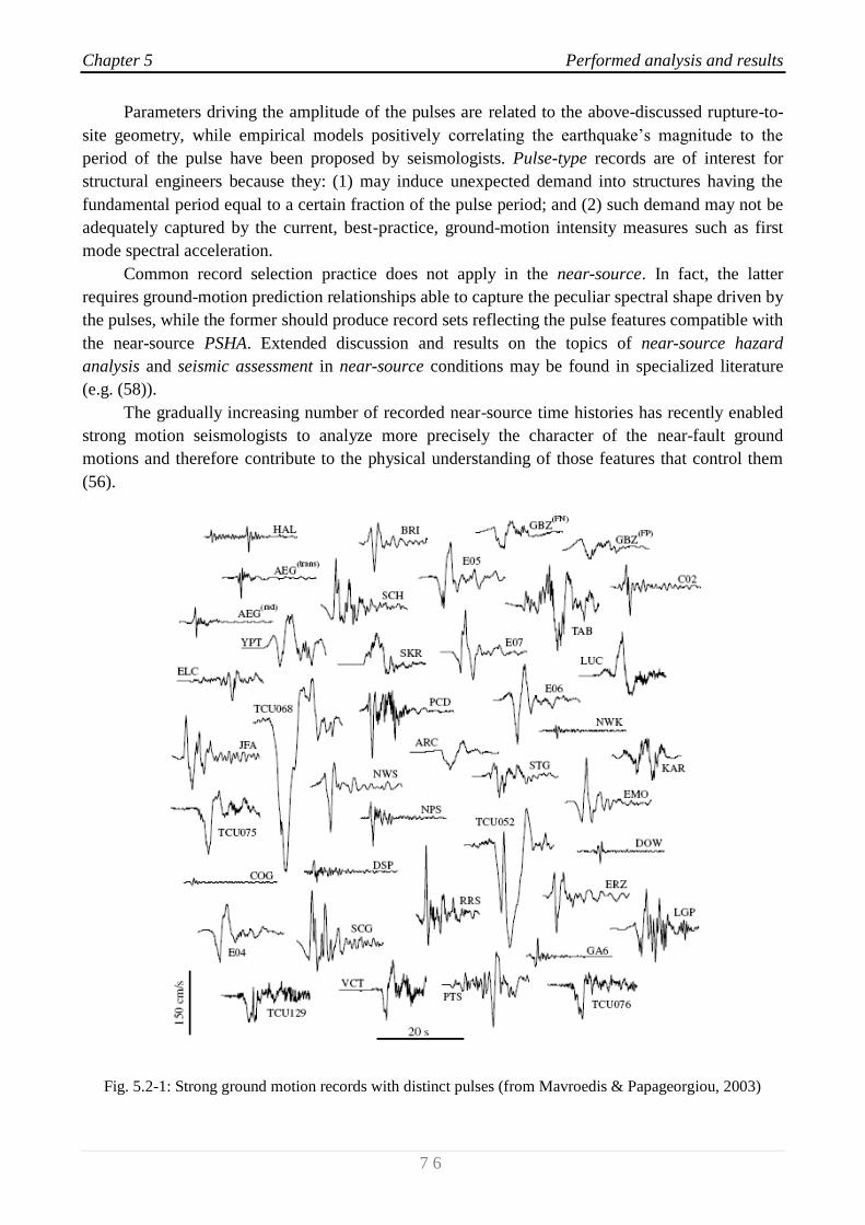
Chapter 5 Performed analysis and results
7 6
Parameters driving the amplitude of the pulses are related to the above-discussed rupture-to-
site geometry, while empirical models positively correlating the earthquake’s magnitude to the
period of the pulse have been proposed by seismologists. Pulse-type records are of interest for
structural engineers because they: (1) may induce unexpected demand into structures having the
fundamental period equal to a certain fraction of the pulse period; and (2) such demand may not be
adequately captured by the current, best-practice, ground-motion intensity measures such as first
mode spectral acceleration.
Common record selection practice does not apply in the near-source. In fact, the latter
requires ground-motion prediction relationships able to capture the peculiar spectral shape driven by
the pulses, while the former should produce record sets reflecting the pulse features compatible with
the near-source PSHA. Extended discussion and results on the topics of near-source hazard
analysis and seismic assessment in near-source conditions may be found in specialized literature
(e.g. (58)).
The gradually increasing number of recorded near-source time histories has recently enabled
strong motion seismologists to analyze more precisely the character of the near-fault ground
motions and therefore contribute to the physical understanding of those features that control them
(56).
Fig. 5.2-1: Strong ground motion records with distinct pulses (from Mavroedis & Papageorgiou, 2003)
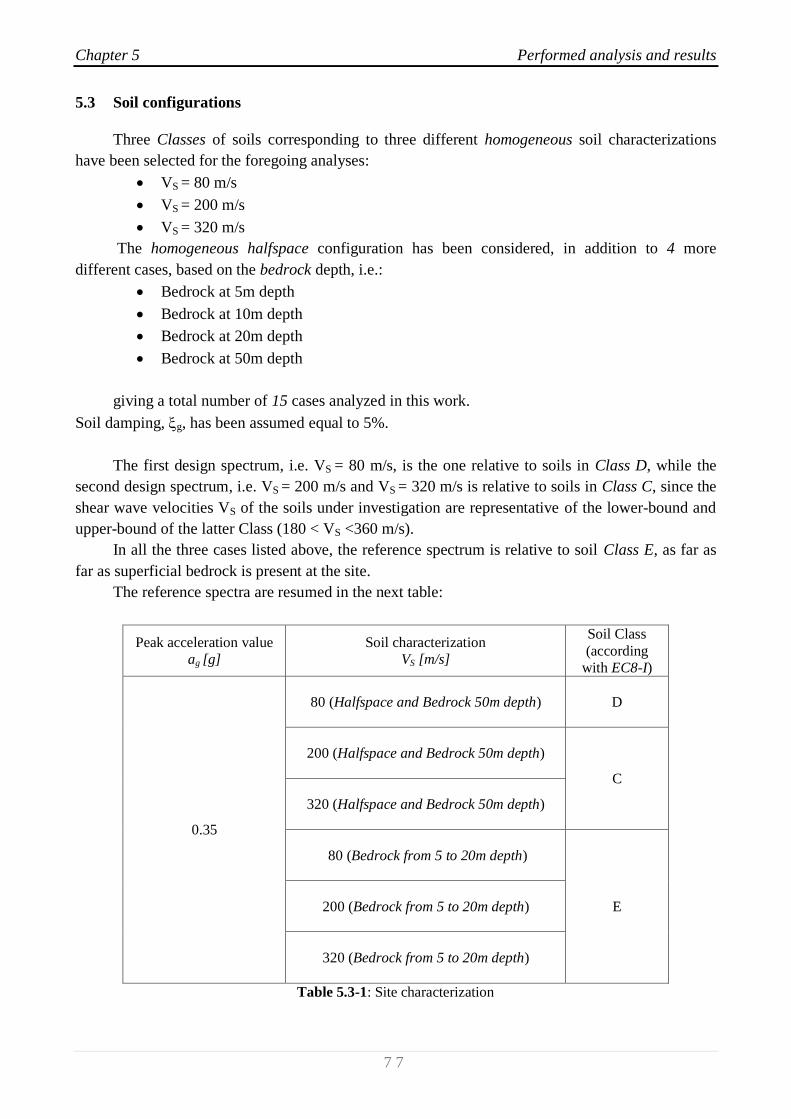
Chapter 5 Performed analysis and results
7 7
5.3 Soil configurations
Three Classes of soils corresponding to three different homogeneous soil characterizations
have been selected for the foregoing analyses:
VS = 80 m/s
VS = 200 m/s
VS = 320 m/s
The homogeneous halfspace configuration has been considered, in addition to 4 more
different cases, based on the bedrock depth, i.e.:
Bedrock at 5m depth
Bedrock at 10m depth
Bedrock at 20m depth
Bedrock at 50m depth
giving a total number of 15 cases analyzed in this work.
Soil damping, g, has been assumed equal to 5%.
The first design spectrum, i.e. VS = 80 m/s, is the one relative to soils in Class D, while the
second design spectrum, i.e. VS = 200 m/s and VS = 320 m/s is relative to soils in Class C, since the
shear wave velocities VS of the soils under investigation are representative of the lower-bound and
upper-bound of the latter Class (180 < VS <360 m/s).
In all the three cases listed above, the reference spectrum is relative to soil Class E, as far as
far as superficial bedrock is present at the site.
The reference spectra are resumed in the next table:
Peak acceleration value
ag [g]
Soil characterization
VS [m/s]
Soil Class
(according
with EC8-I)
0.35
80 (Halfspace and Bedrock 50m depth)
D
200 (Halfspace and Bedrock 50m depth)
C
320 (Halfspace and Bedrock 50m depth)
80 (Bedrock from 5 to 20m depth)
E
200 (Bedrock from 5 to 20m depth)
320 (Bedrock from 5 to 20m depth)
Table 5.3-1: Site characterization

Chapter 5 Performed analysis and results
7 8
5.4 Selected Shear-Buildings
Different ordinary concrete shear-building configurations have been selected in order to
perform the analyses; a general 3D model of the buildings under investigation is displayed in fig.
5.4-1.
Fig. 5.4-1: General 3D model
For this doctoral work, the analyses have been restricted to twelve different building
configurations, such as:
number of storeys: 2, 5, 10, 20
number of bays: 2x2, 5x5, 10x10
squared superficial foundation
The 2D model is represented in fig. 5.4-2
Fig. 5.4-2: General 2D model
Storey height,
H = 3m
Bay length,
B = 5m
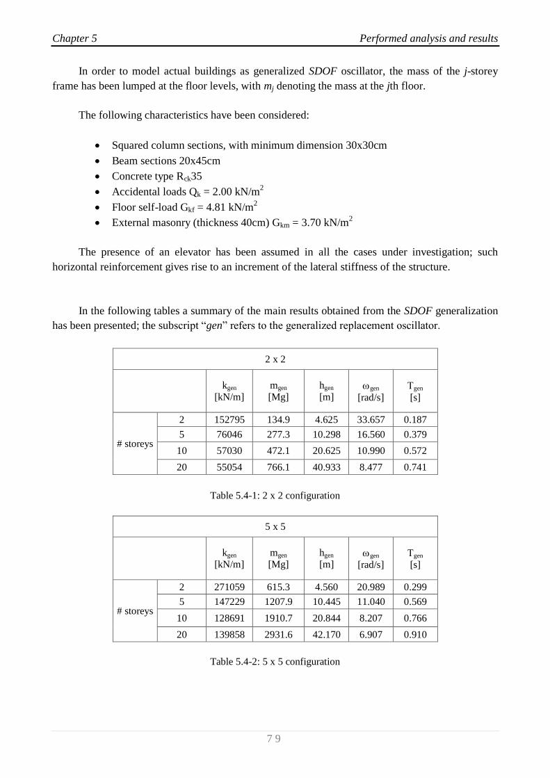
Chapter 5 Performed analysis and results
7 9
In order to model actual buildings as generalized SDOF oscillator, the mass of the j-storey
frame has been lumped at the floor levels, with mj denoting the mass at the jth floor.
The following characteristics have been considered:
Squared column sections, with minimum dimension 30x30cm
Beam sections 20x45cm
Concrete type Rck35
Accidental loads Qk = 2.00 kN/m2
Floor self-load Gkf = 4.81 kN/m2
External masonry (thickness 40cm) Gkm = 3.70 kN/m2
The presence of an elevator has been assumed in all the cases under investigation; such
horizontal reinforcement gives rise to an increment of the lateral stiffness of the structure.
In the following tables a summary of the main results obtained from the SDOF generalization
has been presented; the subscript “gen” refers to the generalized replacement oscillator.
2 x 2
kgen
[kN/m] mgen
[Mg] hgen
[m] gen
[rad/s] gen [s]
# storeys
2 152795 134.9 4.625 33.657 0.187
5 76046 277.3 10.298 16.560 0.379
10 57030 472.1 20.625 10.990 0.572
20 55054 766.1 40.933 8.477 0.741
Table 5.4-1: 2 x 2 configuration
5 x 5
kgen
[kN/m] mgen
[Mg] hgen
[m] gen
[rad/s] gen [s]
# storeys
2 271059 615.3 4.560 20.989 0.299
5 147229 1207.9 10.445 11.040 0.569
10 128691 1910.7 20.844 8.207 0.766
20 139858 2931.6 42.170 6.907 0.910
Table 5.4-2: 5 x 5 configuration
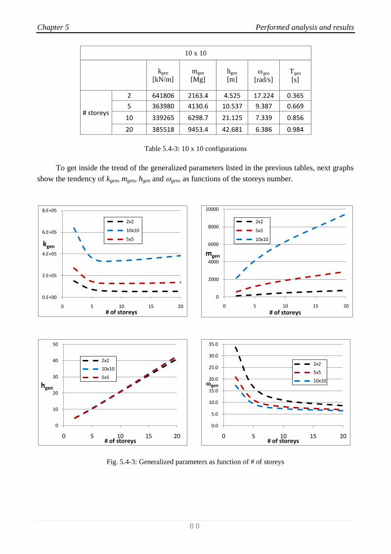
Chapter 5 Performed analysis and results
8 0
10 x 10
kgen
[kN/m] mgen
[Mg] hgen
[m] gen
[rad/s] gen [s]
# storeys
2 641806 2163.4 4.525 17.224 0.365
5 363980 4130.6 10.537 9.387 0.669
10 339265 6298.7 21.125 7.339 0.856
20 385518 9453.4 42.681 6.386 0.984
Table 5.4-3: 10 x 10 configurations
To get inside the trend of the generalized parameters listed in the previous tables, next graphs
show the tendency of kgen, mgen, hgen and gen, as functions of the storeys number.
Fig. 5.4-3: Generalized parameters as function of # of storeys
0.E+00
2.E+05
4.E+05
6.E+05
8.E+05
0 5 10 15 20
kgen
# of storeys
2x2
10x10
5x5
0
2000
4000
6000
8000
10000
0 5 10 15 20
mgen
# of storeys
2x2
5x5
10x10
0
10
20
30
40
50
0 5 10 15 20
hgen
# of storeys
2x2
10x10
5x5
0.0
5.0
10.0
15.0
20.0
25.0
30.0
35.0
0 5 10 15 20
gen
# of storeys
2x2
5x5
10x10
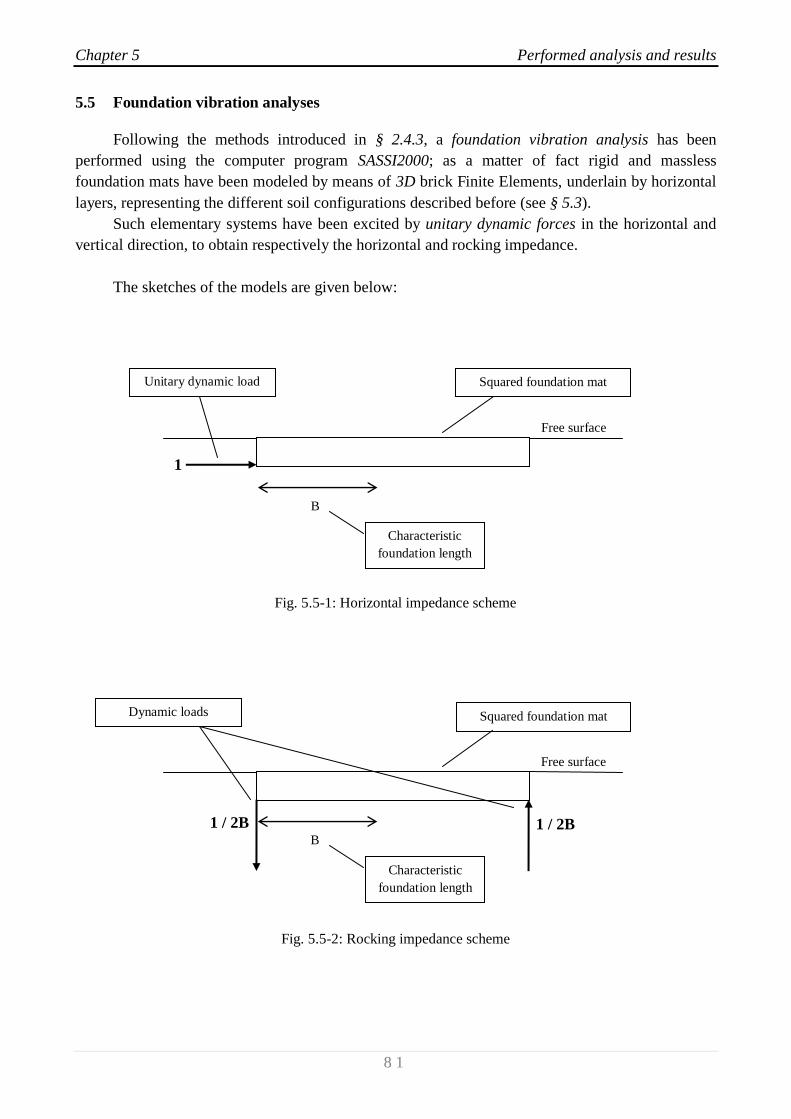
Chapter 5 Performed analysis and results
8 1
Free surface
B
1
Free surface
B
1 / 2B 1 / 2B
5.5 Foundation vibration analyses
Following the methods introduced in § 2.4.3, a foundation vibration analysis has been
performed using the computer program SASSI2000; as a matter of fact rigid and massless
foundation mats have been modeled by means of 3D brick Finite Elements, underlain by horizontal
layers, representing the different soil configurations described before (see § 5.3).
Such elementary systems have been excited by unitary dynamic forces in the horizontal and
vertical direction, to obtain respectively the horizontal and rocking impedance.
The sketches of the models are given below:
Fig. 5.5-1: Horizontal impedance scheme
Fig. 5.5-2: Rocking impedance scheme
Squared foundation mat Unitary dynamic load
Characteristic
foundation length
Squared foundation mat Dynamic loads
Characteristic
foundation length

Chapter 5 Performed analysis and results
8 2
The frequency dependent dynamic stiffnesses and total (radiation + material)
dampings for the case of horizontal and rotational dynamic movements have been evaluated
for all the above cases of interests; in consequence the following 45 analyses have been performed:
Vs [m/s]
Superficial foundation 80 200 320
15
cases 2x2 (10x10m)
Halfspace
Bedrock 5m
Bedrock 10m
Bedrock 20m
Bedrock 50m
Table 5.5-1: 2x2 foundation configuration
Vs [m/s]
Superficial foundation 80 200 320
15
cases 5x5 (25x25m)
Halfspace
Bedrock 5m
Bedrock 10m
Bedrock 20m
Bedrock 50m
Table 5.5-2: 5x5 foundation configuration
Vs [m/s]
Superficial foundation 80 200 320
15
cases 10x10 (50x50m)
Halfspace
Bedrock 5m
Bedrock 10m
Bedrock 20m
Bedrock 50m
Table 5.5-3: 10x10 foundation configuration
For the sake of conciseness, only the results for the 2x2 building resting on a soil with
Vs = 80 m/s, are presented hereinafter, while the complete results are resumed in Appendix A.

Chapter 5 Performed analysis and results
8 3
In the next plots, dynamic horizontal, khh, and rocking, krr , stiffnesses are presented as a
function of the frequency dimensionless parameter
.
As pointed out in § 2.6, for practical applications in earthquake engineering, dimensionless
frequencies in the range 0 ≤ ≤ 2 are usually considered. Values greater than 2 are far from typical
frequencies generated during earthquake shakings; so, in the next charts the trend of previous
frequency dependent parameters will be showed within this range.
Fig. 5.5-3: Horizontal dynamic stiffness (function of a0)
Fig. 5.5-4: Rocking dynamic stiffness (function of a0)
From the charts showed above, it is easy to observe the convergence between a configuration
with deep bedrock and the halfspace; in fact, as the bedrock goes deeper, the approximation with
the halfspace is good.
0.E+00
1.E+05
2.E+05
3.E+05
4.E+05
5.E+05
6.E+05
7.E+05
0.0 0.5 1.0 1.5 2.0
k hh
[kN
/m]
a0
Vs = 80 m/sHalfspace
Bedrock 5m
Bedrock 10m
Bedrock 20m
Bedrock 50m
0.E+00
2.E+06
4.E+06
6.E+06
8.E+06
1.E+07
1.E+07
1.E+07
2.E+07
0.0 0.5 1.0 1.5 2.0
k rr[k
Ns/
m]
a0
Vs = 80 m/s
Halfspace
Bedrock 5m
Bedrock 10m
Bedrock 20m
Bedrock 50m
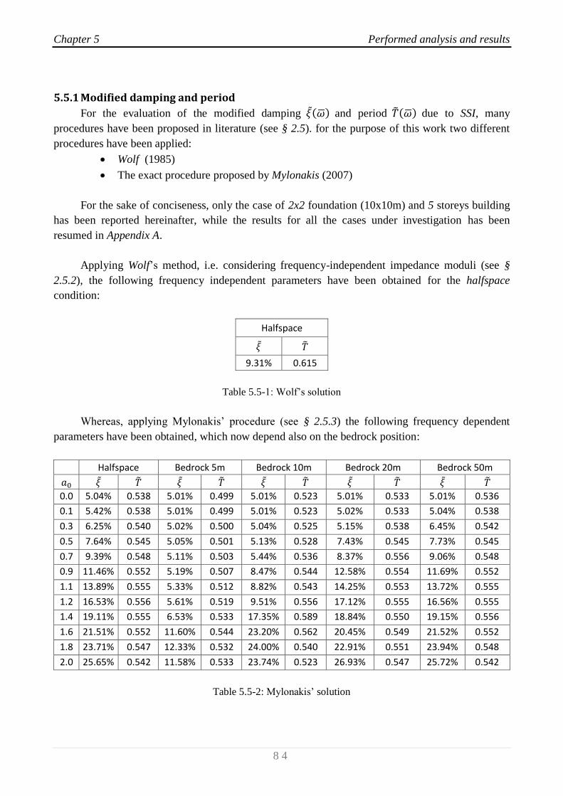
Chapter 5 Performed analysis and results
8 4
5.5.1 Modified damping and period
For the evaluation of the modified damping and period due to SSI, many
procedures have been proposed in literature (see § 2.5). for the purpose of this work two different
procedures have been applied:
Wolf (1985)
The exact procedure proposed by Mylonakis (2007)
For the sake of conciseness, only the case of 2x2 foundation (10x10m) and 5 storeys building
has been reported hereinafter, while the results for all the cases under investigation has been
resumed in Appendix A.
Applying Wolf’s method, i.e. considering frequency-independent impedance moduli (see §
2.5.2), the following frequency independent parameters have been obtained for the halfspace
condition:
Halfspace
9.31% 0.615
Table 5.5-1: Wolf’s solution
Whereas, applying Mylonakis’ procedure (see § 2.5.3) the following frequency dependent
parameters have been obtained, which now depend also on the bedrock position:
Halfspace Bedrock 5m Bedrock 10m Bedrock 20m Bedrock 50m
0.0 5.04% 0.538 5.01% 0.499 5.01% 0.523 5.01% 0.533 5.01% 0.536
0.1 5.42% 0.538 5.01% 0.499 5.01% 0.523 5.02% 0.533 5.04% 0.538
0.3 6.25% 0.540 5.02% 0.500 5.04% 0.525 5.15% 0.538 6.45% 0.542
0.5 7.64% 0.545 5.05% 0.501 5.13% 0.528 7.43% 0.545 7.73% 0.545
0.7 9.39% 0.548 5.11% 0.503 5.44% 0.536 8.37% 0.556 9.06% 0.548
0.9 11.46% 0.552 5.19% 0.507 8.47% 0.544 12.58% 0.554 11.69% 0.552
1.1 13.89% 0.555 5.33% 0.512 8.82% 0.543 14.25% 0.553 13.72% 0.555
1.2 16.53% 0.556 5.61% 0.519 9.51% 0.556 17.12% 0.555 16.56% 0.555
1.4 19.11% 0.555 6.53% 0.533 17.35% 0.589 18.84% 0.550 19.15% 0.556
1.6 21.51% 0.552 11.60% 0.544 23.20% 0.562 20.45% 0.549 21.52% 0.552
1.8 23.71% 0.547 12.33% 0.532 24.00% 0.540 22.91% 0.551 23.94% 0.548
2.0 25.65% 0.542 11.58% 0.533 23.74% 0.523 26.93% 0.547 25.72% 0.542
Table 5.5-2: Mylonakis’ solution

Chapter 5 Performed analysis and results
8 5
With Mylonakis’ solution, results are not only frequency dependent (a great improvement
comparing with Wolf solution, but they show dependence also in the deposit configuration.
Such differences can be easily checked in the next graphs, where the trend of and are
shown as function of the dimensionless frequency parameter, a0.
In dotted lines, classical solution of fixed-base condition is presented as a limiting case of the
analysis.
Fig. 5.5-5: Comparison of modified dampings
Fig. 5.5-6: Comparison of modified periods
In all the graphs presented in this paragraph, the undulations of solutions are due to the strong
dependence on the depth of the bedrock. On a stratum, , is not a smooth function but exhibits
peaks and valleys associated with the natural frequencies (in shearing and compression–extension)
of the stratum (see § 2.4.3).
0%
5%
10%
15%
20%
25%
30%
0.0 0.5 1.0 1.5 2.0
a0
5 - StoreysMylonakis - Halfspace
Wolf
Mylonakis - Bedrock 5m
Mylonakis - Bedrock 10m
Mylonakis - Bedrock 20m
Mylonakis - Bedrock 50m
Fixed Base
0.10
0.20
0.30
0.40
0.50
0.60
0.70
0.0 0.5 1.0 1.5 2.0
T
a0
5 - Storeys
Mylonakis - Halfspace
Wolf
Mylonakis - Bedrock 5m
Mylonakis - Bedrock 10m
Mylonakis - Bedrock 20m
Mylonakis - Bedrock 50m
Fixed-Base

Chapter 5 Performed analysis and results
8 6
5.5.2 Simplified dimensionless charts
The first objective of this doctoral work is to create dimensionless charts for the practical
application of SSI. To this end, for each case under investigation, the classical dimensionless
parameter (see §2.6) has been evaluated.
2x2
h / r
1 /
Vs = 80
m/s
1 /
Vs = 200
m/s
1 /
Vs = 320
m/s
# storeys
2 0.9 1.89 0.19 0.31 0.12 0.08
5 2.1 0.92 0.18 0.34 0.14 0.08
10 4.1 0.54 0.15 0.45 0.18 0.11
20 8.2 0.33 0.12 0.69 0.28 0.17
Table 5.5-3: Dimensionless parameters (2x2 case)
5x5
h / r
1 /
Vs = 80
m/s
1 /
Vs = 200
m/s
1 /
Vs = 320
m/s
# storeys
2 0.4 2.59 0.14 0.19 0.08 0.05
5 0.8 1.32 0.12 0.23 0.09 0.06
10 1.7 0.83 0.10 0.34 0.14 0.09
20 3.4 0.54 0.07 0.58 0.23 0.14
Table 5.5-4: Dimensionless parameters (5x5 case)
10x10
h / r
1 /
Vs = 80
m/s
1 /
Vs = 200
m/s
1 /
Vs = 320
m/s
# storeys
2 0.2 2.94 0.13 0.16 0.06 0.04
5 0.4 1.54 0.10 0.20 0.08 0.05
10 0.8 1.01 0.08 0.31 0.12 0.08
20 1.7 0.67 0.06 0.54 0.22 0.14
Table 5.5-5: Dimensionless parameters (10x10 case)
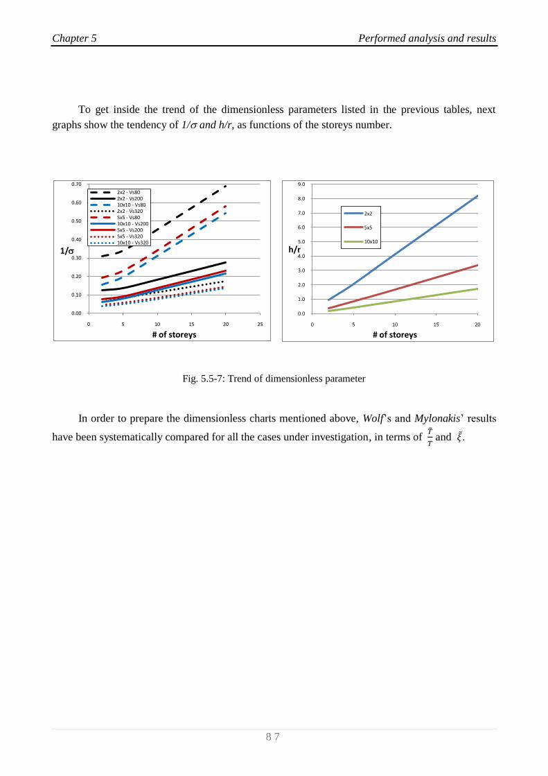
Chapter 5 Performed analysis and results
8 7
To get inside the trend of the dimensionless parameters listed in the previous tables, next
graphs show the tendency of 1/ and h/r, as functions of the storeys number.
Fig. 5.5-7: Trend of dimensionless parameter
In order to prepare the dimensionless charts mentioned above, Wolf’s and Mylonakis’ results
have been systematically compared for all the cases under investigation, in terms of
and .
0.00
0.10
0.20
0.30
0.40
0.50
0.60
0.70
0 5 10 15 20 25
1/
# of storeys
2x2 - Vs802x2 - Vs20010x10 - Vs802x2 - Vs3205x5 - Vs8010x10 - Vs2005x5 - Vs2005x5 - Vs32010x10 - Vs320
0.0
1.0
2.0
3.0
4.0
5.0
6.0
7.0
8.0
9.0
0 5 10 15 20
h/r
# of storeys
2x2
5x5
10x10

Chapter 5 Performed analysis and results
8 8
Results for buildings 2x2
Building type # of storeys VS [m/s] h/r 1/
2x2 2 80 0.9 0.31
Wolf (Halfspace)
Mylonakis (Halfspace)
Mylonakis (Bedrock 5m)
Mylonakis (Bedrock 10m)
Mylonakis (Bedrock 20m)
Mylonakis (Bedrock 50m)
(%) (%) (%) (%) (%) (%)
0.0 1.44 18.50 1.33 5.08 1.23 5.01 1.28 5.01 1.30 5.01 1.32 5.01
0.1 1.44 18.50 1.33 5.92 1.23 5.01 1.28 5.01 1.30 5.02 1.32 5.06
0.3 1.44 18.50 1.33 7.43 1.23 5.02 1.28 5.05 1.32 5.24 1.33 7.89
0.5 1.44 18.50 1.33 9.46 1.23 5.06 1.29 5.18 1.34 10.34 1.33 9.61
0.7 1.44 18.50 1.33 11.34 1.24 5.13 1.32 5.74 1.34 10.79 1.32 10.61
0.9 1.44 18.50 1.32 13.01 1.25 5.24 1.35 12.56 1.32 13.93 1.32 13.60
1.1 1.44 18.50 1.32 14.79 1.27 5.45 1.30 13.15 1.31 14.29 1.32 14.38
1.2 1.44 18.50 1.31 16.61 1.29 5.94 1.30 12.53 1.32 17.82 1.30 16.71
1.4 1.44 18.50 1.30 18.12 1.35 7.72 1.34 16.35 1.28 18.29 1.30 18.26
1.6 1.44 18.50 1.28 19.28 1.41 18.87 1.28 19.40 1.27 17.78 1.28 19.22
1.8 1.44 18.50 1.27 20.27 1.31 21.86 1.24 18.52 1.28 18.65 1.27 20.68
2.0 1.44 18.50 1.25 21.13 1.26 19.57 1.21 17.15 1.27 23.49 1.25 21.16
Building type # of storeys VS [m/s] h/r 1/
2x2 5 80 2.1 0.34
Wolf
(Halfspace) Mylonakis (Halfspace)
Mylonakis (Bedrock 5m)
Mylonakis (Bedrock 10m)
Mylonakis (Bedrock 20m)
Mylonakis (Bedrock 50m)
(%) (%) (%) (%) (%) (%)
0.0 1.62 9.31 1.42 5.04 1.31 5.01 1.38 5.01 1.40 5.01 1.41 5.01
0.1 1.62 9.31 1.42 5.42 1.31 5.01 1.38 5.01 1.41 5.02 1.42 5.04
0.3 1.62 9.31 1.42 6.25 1.32 5.02 1.38 5.04 1.42 5.15 1.43 6.45
0.5 1.62 9.31 1.44 7.64 1.32 5.05 1.39 5.13 1.44 7.43 1.44 7.73
0.7 1.62 9.31 1.45 9.39 1.33 5.11 1.41 5.44 1.47 8.37 1.45 9.06
0.9 1.62 9.31 1.46 11.46 1.34 5.19 1.43 8.47 1.46 12.58 1.45 11.69
1.1 1.62 9.31 1.46 13.89 1.35 5.33 1.43 8.82 1.46 14.25 1.46 13.72
1.2 1.62 9.31 1.46 16.53 1.37 5.61 1.47 9.51 1.46 17.12 1.46 16.56
1.4 1.62 9.31 1.46 19.11 1.40 6.53 1.55 17.35 1.45 18.84 1.46 19.15
1.6 1.62 9.31 1.45 21.51 1.43 11.60 1.48 23.20 1.45 20.45 1.45 21.52
1.8 1.62 9.31 1.44 23.71 1.40 12.33 1.42 24.00 1.45 22.91 1.44 23.94
2.0 1.62 9.31 1.43 25.65 1.40 11.58 1.38 23.74 1.44 26.93 1.43 25.72
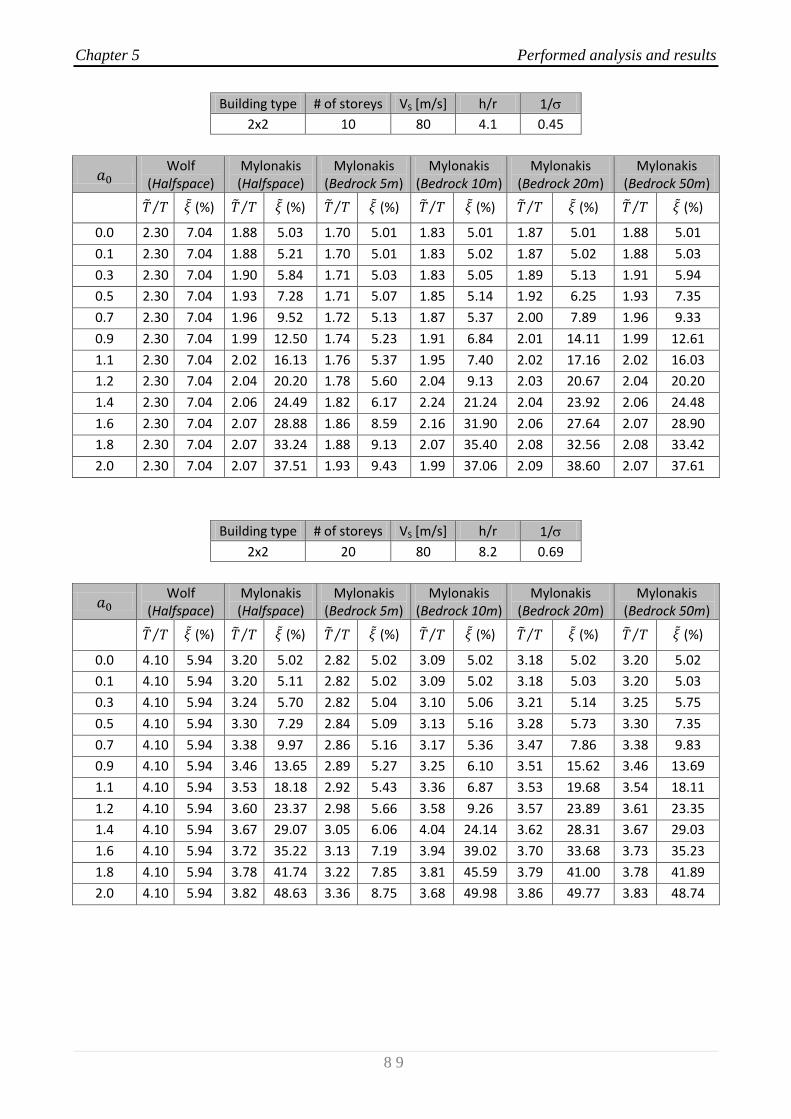
Chapter 5 Performed analysis and results
8 9
Building type # of storeys VS [m/s] h/r 1/
2x2 10 80 4.1 0.45
Wolf
(Halfspace) Mylonakis (Halfspace)
Mylonakis (Bedrock 5m)
Mylonakis (Bedrock 10m)
Mylonakis (Bedrock 20m)
Mylonakis (Bedrock 50m)
(%) (%) (%) (%) (%) (%)
0.0 2.30 7.04 1.88 5.03 1.70 5.01 1.83 5.01 1.87 5.01 1.88 5.01
0.1 2.30 7.04 1.88 5.21 1.70 5.01 1.83 5.02 1.87 5.02 1.88 5.03
0.3 2.30 7.04 1.90 5.84 1.71 5.03 1.83 5.05 1.89 5.13 1.91 5.94
0.5 2.30 7.04 1.93 7.28 1.71 5.07 1.85 5.14 1.92 6.25 1.93 7.35
0.7 2.30 7.04 1.96 9.52 1.72 5.13 1.87 5.37 2.00 7.89 1.96 9.33
0.9 2.30 7.04 1.99 12.50 1.74 5.23 1.91 6.84 2.01 14.11 1.99 12.61
1.1 2.30 7.04 2.02 16.13 1.76 5.37 1.95 7.40 2.02 17.16 2.02 16.03
1.2 2.30 7.04 2.04 20.20 1.78 5.60 2.04 9.13 2.03 20.67 2.04 20.20
1.4 2.30 7.04 2.06 24.49 1.82 6.17 2.24 21.24 2.04 23.92 2.06 24.48
1.6 2.30 7.04 2.07 28.88 1.86 8.59 2.16 31.90 2.06 27.64 2.07 28.90
1.8 2.30 7.04 2.07 33.24 1.88 9.13 2.07 35.40 2.08 32.56 2.08 33.42
2.0 2.30 7.04 2.07 37.51 1.93 9.43 1.99 37.06 2.09 38.60 2.07 37.61
Building type # of storeys VS [m/s] h/r 1/
2x2 20 80 8.2 0.69
Wolf
(Halfspace) Mylonakis (Halfspace)
Mylonakis (Bedrock 5m)
Mylonakis (Bedrock 10m)
Mylonakis (Bedrock 20m)
Mylonakis (Bedrock 50m)
(%) (%) (%) (%) (%) (%)
0.0 4.10 5.94 3.20 5.02 2.82 5.02 3.09 5.02 3.18 5.02 3.20 5.02
0.1 4.10 5.94 3.20 5.11 2.82 5.02 3.09 5.02 3.18 5.03 3.20 5.03
0.3 4.10 5.94 3.24 5.70 2.82 5.04 3.10 5.06 3.21 5.14 3.25 5.75
0.5 4.10 5.94 3.30 7.29 2.84 5.09 3.13 5.16 3.28 5.73 3.30 7.35
0.7 4.10 5.94 3.38 9.97 2.86 5.16 3.17 5.36 3.47 7.86 3.38 9.83
0.9 4.10 5.94 3.46 13.65 2.89 5.27 3.25 6.10 3.51 15.62 3.46 13.69
1.1 4.10 5.94 3.53 18.18 2.92 5.43 3.36 6.87 3.53 19.68 3.54 18.11
1.2 4.10 5.94 3.60 23.37 2.98 5.66 3.58 9.26 3.57 23.89 3.61 23.35
1.4 4.10 5.94 3.67 29.07 3.05 6.06 4.04 24.14 3.62 28.31 3.67 29.03
1.6 4.10 5.94 3.72 35.22 3.13 7.19 3.94 39.02 3.70 33.68 3.73 35.23
1.8 4.10 5.94 3.78 41.74 3.22 7.85 3.81 45.59 3.79 41.00 3.78 41.89
2.0 4.10 5.94 3.82 48.63 3.36 8.75 3.68 49.98 3.86 49.77 3.83 48.74
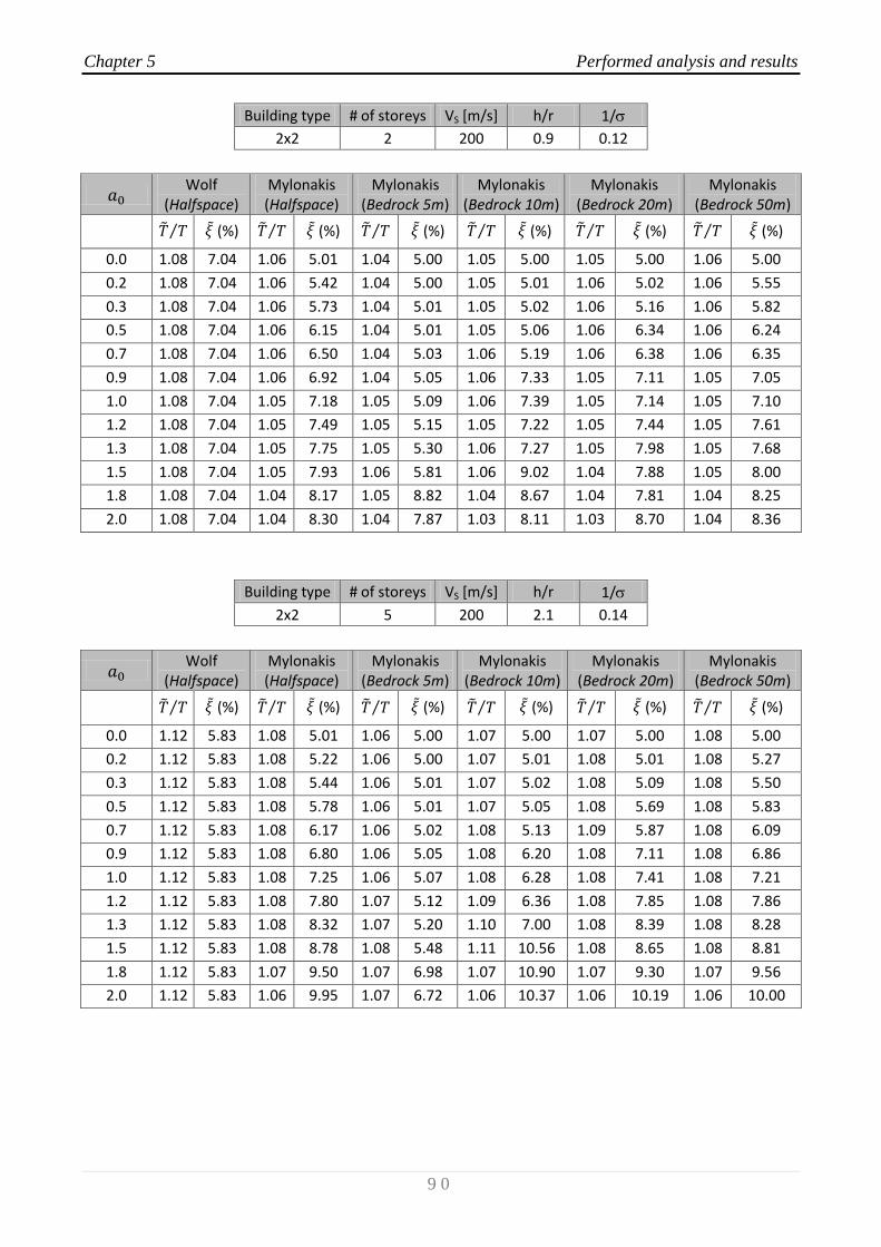
Chapter 5 Performed analysis and results
9 0
Building type # of storeys VS [m/s] h/r 1/
2x2 2 200 0.9 0.12
Wolf
(Halfspace) Mylonakis (Halfspace)
Mylonakis (Bedrock 5m)
Mylonakis (Bedrock 10m)
Mylonakis (Bedrock 20m)
Mylonakis (Bedrock 50m)
(%) (%) (%) (%) (%) (%)
0.0 1.08 7.04 1.06 5.01 1.04 5.00 1.05 5.00 1.05 5.00 1.06 5.00
0.2 1.08 7.04 1.06 5.42 1.04 5.00 1.05 5.01 1.06 5.02 1.06 5.55
0.3 1.08 7.04 1.06 5.73 1.04 5.01 1.05 5.02 1.06 5.16 1.06 5.82
0.5 1.08 7.04 1.06 6.15 1.04 5.01 1.05 5.06 1.06 6.34 1.06 6.24
0.7 1.08 7.04 1.06 6.50 1.04 5.03 1.06 5.19 1.06 6.38 1.06 6.35
0.9 1.08 7.04 1.06 6.92 1.04 5.05 1.06 7.33 1.05 7.11 1.05 7.05
1.0 1.08 7.04 1.05 7.18 1.05 5.09 1.06 7.39 1.05 7.14 1.05 7.10
1.2 1.08 7.04 1.05 7.49 1.05 5.15 1.05 7.22 1.05 7.44 1.05 7.61
1.3 1.08 7.04 1.05 7.75 1.05 5.30 1.06 7.27 1.05 7.98 1.05 7.68
1.5 1.08 7.04 1.05 7.93 1.06 5.81 1.06 9.02 1.04 7.88 1.05 8.00
1.8 1.08 7.04 1.04 8.17 1.05 8.82 1.04 8.67 1.04 7.81 1.04 8.25
2.0 1.08 7.04 1.04 8.30 1.04 7.87 1.03 8.11 1.03 8.70 1.04 8.36
Building type # of storeys VS [m/s] h/r 1/
2x2 5 200 2.1 0.14
Wolf
(Halfspace) Mylonakis (Halfspace)
Mylonakis (Bedrock 5m)
Mylonakis (Bedrock 10m)
Mylonakis (Bedrock 20m)
Mylonakis (Bedrock 50m)
(%) (%) (%) (%) (%) (%)
0.0 1.12 5.83 1.08 5.01 1.06 5.00 1.07 5.00 1.07 5.00 1.08 5.00
0.2 1.12 5.83 1.08 5.22 1.06 5.00 1.07 5.01 1.08 5.01 1.08 5.27
0.3 1.12 5.83 1.08 5.44 1.06 5.01 1.07 5.02 1.08 5.09 1.08 5.50
0.5 1.12 5.83 1.08 5.78 1.06 5.01 1.07 5.05 1.08 5.69 1.08 5.83
0.7 1.12 5.83 1.08 6.17 1.06 5.02 1.08 5.13 1.09 5.87 1.08 6.09
0.9 1.12 5.83 1.08 6.80 1.06 5.05 1.08 6.20 1.08 7.11 1.08 6.86
1.0 1.12 5.83 1.08 7.25 1.06 5.07 1.08 6.28 1.08 7.41 1.08 7.21
1.2 1.12 5.83 1.08 7.80 1.07 5.12 1.09 6.36 1.08 7.85 1.08 7.86
1.3 1.12 5.83 1.08 8.32 1.07 5.20 1.10 7.00 1.08 8.39 1.08 8.28
1.5 1.12 5.83 1.08 8.78 1.08 5.48 1.11 10.56 1.08 8.65 1.08 8.81
1.8 1.12 5.83 1.07 9.50 1.07 6.98 1.07 10.90 1.07 9.30 1.07 9.56
2.0 1.12 5.83 1.06 9.95 1.07 6.72 1.06 10.37 1.06 10.19 1.06 10.00

Chapter 5 Performed analysis and results
9 1
Building type # of storeys VS [m/s] h/r 1/
2x2 10 200 4.1 0.18
Wolf
(Halfspace) Mylonakis (Halfspace)
Mylonakis (Bedrock 5m)
Mylonakis (Bedrock 10m)
Mylonakis (Bedrock 20m)
Mylonakis (Bedrock 50m)
(%) (%) (%) (%) (%) (%)
0.0 1.30 5.73 1.19 5.01 1.14 5.00 1.17 5.01 1.18 5.01 1.19 5.01
0.2 1.30 5.73 1.19 5.18 1.14 5.01 1.17 5.01 1.18 5.02 1.19 5.19
0.3 1.30 5.73 1.19 5.48 1.14 5.01 1.18 5.04 1.19 5.10 1.19 5.55
0.5 1.30 5.73 1.20 6.02 1.14 5.03 1.18 5.08 1.20 5.54 1.20 6.05
0.7 1.30 5.73 1.20 6.78 1.15 5.05 1.19 5.17 1.21 6.01 1.20 6.70
0.9 1.30 5.73 1.21 8.14 1.15 5.08 1.20 5.93 1.22 8.82 1.21 8.18
1.0 1.30 5.73 1.21 9.16 1.15 5.12 1.21 6.12 1.21 9.66 1.21 9.13
1.2 1.30 5.73 1.22 10.42 1.16 5.17 1.23 6.53 1.21 10.64 1.22 10.46
1.3 1.30 5.73 1.21 11.68 1.16 5.27 1.27 8.21 1.21 11.68 1.21 11.66
1.5 1.30 5.73 1.21 12.88 1.17 5.50 1.30 16.30 1.21 12.57 1.21 12.90
1.8 1.30 5.73 1.20 14.96 1.18 6.62 1.21 18.77 1.20 14.71 1.20 15.02
2.0 1.30 5.73 1.18 16.43 1.20 6.93 1.17 18.29 1.18 16.73 1.18 16.51
Building type # of storeys VS [m/s] h/r 1/
2x2 20 200 8.2 0.28
Wolf
(Halfspace) Mylonakis (Halfspace)
Mylonakis (Bedrock 5m)
Mylonakis (Bedrock 10m)
Mylonakis (Bedrock 20m)
Mylonakis (Bedrock 50m)
(%) (%) (%) (%) (%) (%)
0.0 1.88 5.62 1.57 5.01 1.45 5.01 1.54 5.01 1.57 5.01 1.57 5.01
0.2 1.88 5.62 1.58 5.20 1.45 5.02 1.54 5.03 1.57 5.04 1.58 5.15
0.3 1.88 5.62 1.59 5.71 1.46 5.03 1.55 5.07 1.58 5.14 1.59 5.82
0.5 1.88 5.62 1.61 6.69 1.46 5.06 1.56 5.15 1.60 5.53 1.61 6.72
0.7 1.88 5.62 1.63 8.15 1.46 5.09 1.57 5.28 1.65 6.52 1.63 8.06
0.9 1.88 5.62 1.65 10.90 1.47 5.17 1.61 5.92 1.67 12.26 1.66 10.92
1.0 1.88 5.62 1.67 13.00 1.48 5.23 1.64 6.30 1.67 14.13 1.67 12.95
1.2 1.88 5.62 1.68 15.63 1.49 5.33 1.69 7.23 1.67 16.22 1.68 15.64
1.3 1.88 5.62 1.69 18.40 1.51 5.47 1.81 10.44 1.68 18.39 1.69 18.37
1.5 1.88 5.62 1.69 21.22 1.53 5.72 1.96 26.03 1.68 20.58 1.69 21.21
1.8 1.88 5.62 1.69 26.72 1.57 6.75 1.79 36.32 1.69 26.18 1.69 26.82
2.0 1.88 5.62 1.67 31.63 1.64 7.84 1.68 38.52 1.67 32.25 1.67 31.77
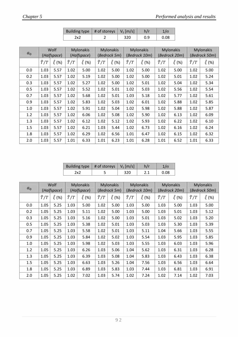
Chapter 5 Performed analysis and results
9 2
Building type # of storeys VS [m/s] h/r 1/
2x2 2 320 0.9 0.08
Wolf
(Halfspace) Mylonakis (Halfspace)
Mylonakis (Bedrock 5m)
Mylonakis (Bedrock 10m)
Mylonakis (Bedrock 20m)
Mylonakis (Bedrock 50m)
(%) (%) (%) (%) (%) (%)
0.0 1.03 5.57 1.02 5.00 1.02 5.00 1.02 5.00 1.02 5.00 1.02 5.00
0.2 1.03 5.57 1.02 5.19 1.02 5.00 1.02 5.00 1.02 5.01 1.02 5.24
0.3 1.03 5.57 1.02 5.27 1.02 5.00 1.02 5.01 1.02 5.04 1.02 5.34
0.5 1.03 5.57 1.02 5.52 1.02 5.01 1.02 5.03 1.02 5.56 1.02 5.54
0.7 1.03 5.57 1.02 5.68 1.02 5.01 1.03 5.18 1.02 5.77 1.02 5.61
0.9 1.03 5.57 1.02 5.83 1.02 5.03 1.02 6.01 1.02 5.88 1.02 5.85
1.0 1.03 5.57 1.02 5.91 1.02 5.04 1.02 5.98 1.02 5.88 1.02 5.87
1.2 1.03 5.57 1.02 6.06 1.02 5.08 1.02 5.90 1.02 6.13 1.02 6.09
1.3 1.03 5.57 1.02 6.12 1.02 5.12 1.02 5.93 1.02 6.22 1.02 6.10
1.5 1.03 5.57 1.02 6.21 1.03 5.44 1.02 6.73 1.02 6.16 1.02 6.24
1.8 1.03 5.57 1.02 6.29 1.02 6.56 1.01 6.47 1.02 6.15 1.02 6.32
2.0 1.03 5.57 1.01 6.33 1.01 6.23 1.01 6.28 1.01 6.52 1.01 6.33
Building type # of storeys VS [m/s] h/r 1/
2x2 5 320 2.1 0.08
Wolf
(Halfspace) Mylonakis (Halfspace)
Mylonakis (Bedrock 5m)
Mylonakis (Bedrock 10m)
Mylonakis (Bedrock 20m)
Mylonakis (Bedrock 50m)
(%) (%) (%) (%) (%) (%)
0.0 1.05 5.25 1.03 5.00 1.02 5.00 1.03 5.00 1.03 5.00 1.03 5.00
0.2 1.05 5.25 1.03 5.11 1.02 5.00 1.03 5.00 1.03 5.01 1.03 5.12
0.3 1.05 5.25 1.03 5.16 1.02 5.00 1.03 5.01 1.03 5.02 1.03 5.20
0.5 1.05 5.25 1.03 5.38 1.02 5.01 1.03 5.03 1.03 5.30 1.03 5.39
0.7 1.05 5.25 1.03 5.58 1.02 5.01 1.03 5.11 1.04 5.66 1.03 5.55
0.9 1.05 5.25 1.03 5.84 1.02 5.02 1.03 5.54 1.03 5.95 1.03 5.85
1.0 1.05 5.25 1.03 5.98 1.02 5.03 1.03 5.55 1.03 6.03 1.03 5.96
1.2 1.05 5.25 1.03 6.26 1.03 5.06 1.04 5.62 1.03 6.31 1.03 6.28
1.3 1.05 5.25 1.03 6.39 1.03 5.08 1.04 5.83 1.03 6.43 1.03 6.38
1.5 1.05 5.25 1.03 6.63 1.03 5.26 1.04 7.56 1.03 6.56 1.03 6.64
1.8 1.05 5.25 1.03 6.89 1.03 5.83 1.03 7.44 1.03 6.81 1.03 6.91
2.0 1.05 5.25 1.02 7.02 1.03 5.74 1.02 7.24 1.02 7.14 1.02 7.03
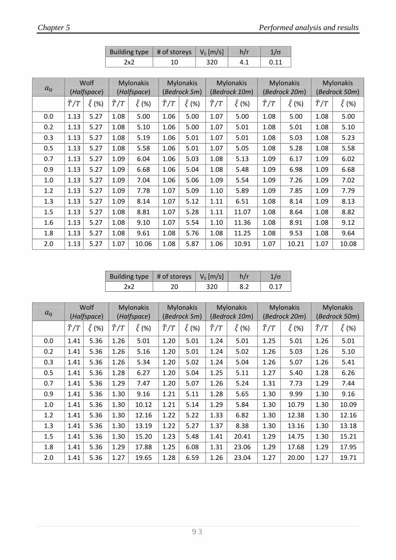
Chapter 5 Performed analysis and results
9 3
Building type # of storeys VS [m/s] h/r 1/
2x2 10 320 4.1 0.11
Wolf
(Halfspace) Mylonakis (Halfspace)
Mylonakis (Bedrock 5m)
Mylonakis (Bedrock 10m)
Mylonakis (Bedrock 20m)
Mylonakis (Bedrock 50m)
(%) (%) (%) (%) (%) (%)
0.0 1.13 5.27 1.08 5.00 1.06 5.00 1.07 5.00 1.08 5.00 1.08 5.00
0.2 1.13 5.27 1.08 5.10 1.06 5.00 1.07 5.01 1.08 5.01 1.08 5.10
0.3 1.13 5.27 1.08 5.19 1.06 5.01 1.07 5.01 1.08 5.03 1.08 5.23
0.5 1.13 5.27 1.08 5.58 1.06 5.01 1.07 5.05 1.08 5.28 1.08 5.58
0.7 1.13 5.27 1.09 6.04 1.06 5.03 1.08 5.13 1.09 6.17 1.09 6.02
0.9 1.13 5.27 1.09 6.68 1.06 5.04 1.08 5.48 1.09 6.98 1.09 6.68
1.0 1.13 5.27 1.09 7.04 1.06 5.06 1.09 5.54 1.09 7.26 1.09 7.02
1.2 1.13 5.27 1.09 7.78 1.07 5.09 1.10 5.89 1.09 7.85 1.09 7.79
1.3 1.13 5.27 1.09 8.14 1.07 5.12 1.11 6.51 1.08 8.14 1.09 8.13
1.5 1.13 5.27 1.08 8.81 1.07 5.28 1.11 11.07 1.08 8.64 1.08 8.82
1.6 1.13 5.27 1.08 9.10 1.07 5.54 1.10 11.36 1.08 8.91 1.08 9.12
1.8 1.13 5.27 1.08 9.61 1.08 5.76 1.08 11.25 1.08 9.53 1.08 9.64
2.0 1.13 5.27 1.07 10.06 1.08 5.87 1.06 10.91 1.07 10.21 1.07 10.08
Building type # of storeys VS [m/s] h/r 1/
2x2 20 320 8.2 0.17
Wolf
(Halfspace) Mylonakis (Halfspace)
Mylonakis (Bedrock 5m)
Mylonakis (Bedrock 10m)
Mylonakis (Bedrock 20m)
Mylonakis (Bedrock 50m)
(%) (%) (%) (%) (%) (%)
0.0 1.41 5.36 1.26 5.01 1.20 5.01 1.24 5.01 1.25 5.01 1.26 5.01
0.2 1.41 5.36 1.26 5.16 1.20 5.01 1.24 5.02 1.26 5.03 1.26 5.10
0.3 1.41 5.36 1.26 5.34 1.20 5.02 1.24 5.04 1.26 5.07 1.26 5.41
0.5 1.41 5.36 1.28 6.27 1.20 5.04 1.25 5.11 1.27 5.40 1.28 6.26
0.7 1.41 5.36 1.29 7.47 1.20 5.07 1.26 5.24 1.31 7.73 1.29 7.44
0.9 1.41 5.36 1.30 9.16 1.21 5.11 1.28 5.65 1.30 9.99 1.30 9.16
1.0 1.41 5.36 1.30 10.12 1.21 5.14 1.29 5.84 1.30 10.79 1.30 10.09
1.2 1.41 5.36 1.30 12.16 1.22 5.22 1.33 6.82 1.30 12.38 1.30 12.16
1.3 1.41 5.36 1.30 13.19 1.22 5.27 1.37 8.38 1.30 13.16 1.30 13.18
1.5 1.41 5.36 1.30 15.20 1.23 5.48 1.41 20.41 1.29 14.75 1.30 15.21
1.8 1.41 5.36 1.29 17.88 1.25 6.08 1.31 23.06 1.29 17.68 1.29 17.95
2.0 1.41 5.36 1.27 19.65 1.28 6.59 1.26 23.04 1.27 20.00 1.27 19.71
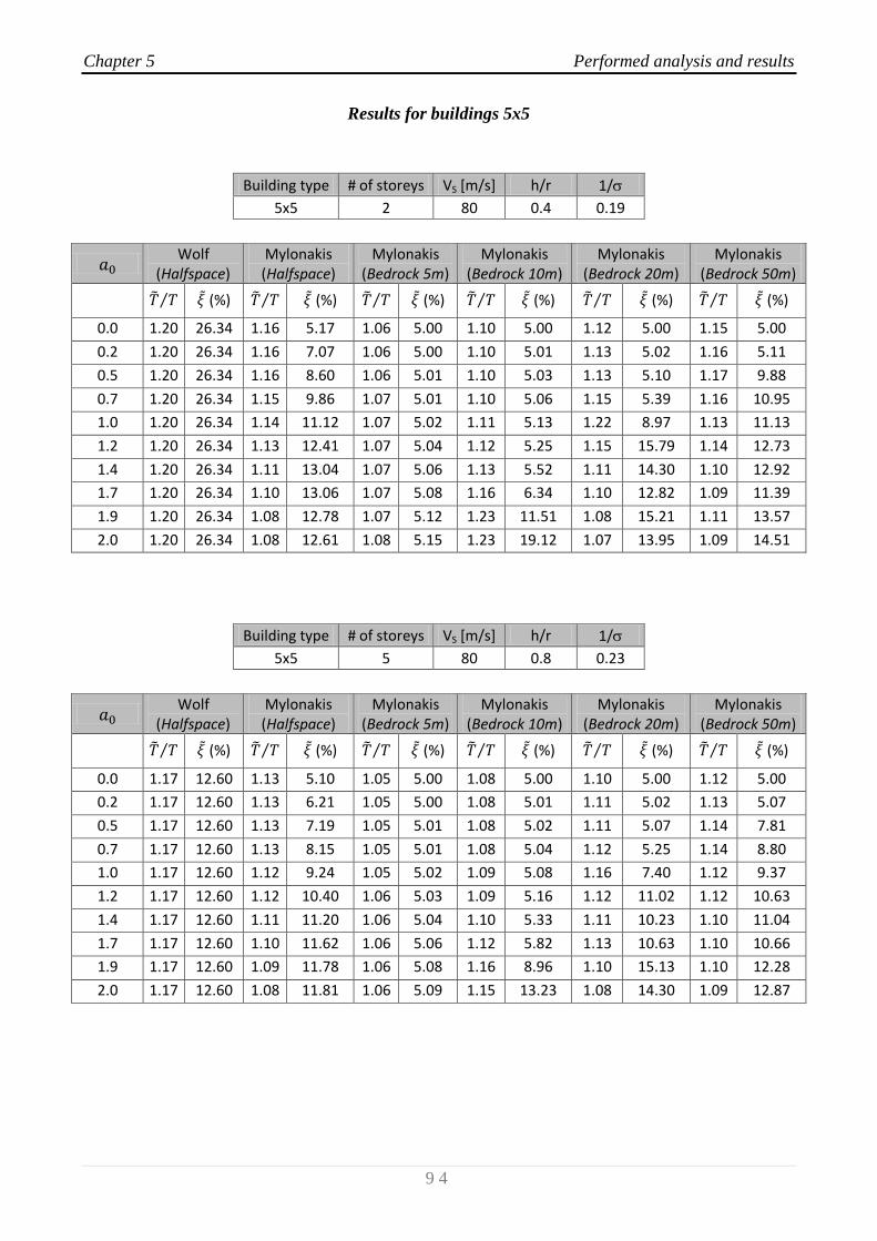
Chapter 5 Performed analysis and results
9 4
Results for buildings 5x5
Building type # of storeys VS [m/s] h/r 1/
5x5 2 80 0.4 0.19
Wolf
(Halfspace) Mylonakis (Halfspace)
Mylonakis (Bedrock 5m)
Mylonakis (Bedrock 10m)
Mylonakis (Bedrock 20m)
Mylonakis (Bedrock 50m)
(%) (%) (%) (%) (%) (%)
0.0 1.20 26.34 1.16 5.17 1.06 5.00 1.10 5.00 1.12 5.00 1.15 5.00
0.2 1.20 26.34 1.16 7.07 1.06 5.00 1.10 5.01 1.13 5.02 1.16 5.11
0.5 1.20 26.34 1.16 8.60 1.06 5.01 1.10 5.03 1.13 5.10 1.17 9.88
0.7 1.20 26.34 1.15 9.86 1.07 5.01 1.10 5.06 1.15 5.39 1.16 10.95
1.0 1.20 26.34 1.14 11.12 1.07 5.02 1.11 5.13 1.22 8.97 1.13 11.13
1.2 1.20 26.34 1.13 12.41 1.07 5.04 1.12 5.25 1.15 15.79 1.14 12.73
1.4 1.20 26.34 1.11 13.04 1.07 5.06 1.13 5.52 1.11 14.30 1.10 12.92
1.7 1.20 26.34 1.10 13.06 1.07 5.08 1.16 6.34 1.10 12.82 1.09 11.39
1.9 1.20 26.34 1.08 12.78 1.07 5.12 1.23 11.51 1.08 15.21 1.11 13.57
2.0 1.20 26.34 1.08 12.61 1.08 5.15 1.23 19.12 1.07 13.95 1.09 14.51
Building type # of storeys VS [m/s] h/r 1/
5x5 5 80 0.8 0.23
Wolf
(Halfspace) Mylonakis (Halfspace)
Mylonakis (Bedrock 5m)
Mylonakis (Bedrock 10m)
Mylonakis (Bedrock 20m)
Mylonakis (Bedrock 50m)
(%) (%) (%) (%) (%) (%)
0.0 1.17 12.60 1.13 5.10 1.05 5.00 1.08 5.00 1.10 5.00 1.12 5.00
0.2 1.17 12.60 1.13 6.21 1.05 5.00 1.08 5.01 1.11 5.02 1.13 5.07
0.5 1.17 12.60 1.13 7.19 1.05 5.01 1.08 5.02 1.11 5.07 1.14 7.81
0.7 1.17 12.60 1.13 8.15 1.05 5.01 1.08 5.04 1.12 5.25 1.14 8.80
1.0 1.17 12.60 1.12 9.24 1.05 5.02 1.09 5.08 1.16 7.40 1.12 9.37
1.2 1.17 12.60 1.12 10.40 1.06 5.03 1.09 5.16 1.12 11.02 1.12 10.63
1.4 1.17 12.60 1.11 11.20 1.06 5.04 1.10 5.33 1.11 10.23 1.10 11.04
1.7 1.17 12.60 1.10 11.62 1.06 5.06 1.12 5.82 1.13 10.63 1.10 10.66
1.9 1.17 12.60 1.09 11.78 1.06 5.08 1.16 8.96 1.10 15.13 1.10 12.28
2.0 1.17 12.60 1.08 11.81 1.06 5.09 1.15 13.23 1.08 14.30 1.09 12.87

Chapter 5 Performed analysis and results
9 5
Building type # of storeys VS [m/s] h/r 1/
5x5 10 80 1.7 0.34
Wolf
(Halfspace) Mylonakis (Halfspace)
Mylonakis (Bedrock 5m)
Mylonakis (Bedrock 10m)
Mylonakis (Bedrock 20m)
Mylonakis (Bedrock 50m)
(%) (%) (%) (%) (%) (%)
0.0 1.33 10.18 1.23 5.08 1.10 5.00 1.16 5.00 1.20 5.01 1.22 5.01
0.2 1.33 10.18 1.23 5.96 1.10 5.00 1.16 5.01 1.20 5.02 1.23 5.07
0.5 1.33 10.18 1.24 7.00 1.10 5.01 1.16 5.02 1.21 5.08 1.24 7.13
0.7 1.33 10.18 1.25 8.42 1.10 5.01 1.16 5.05 1.22 5.25 1.26 8.97
1.0 1.33 10.18 1.25 10.28 1.11 5.02 1.16 5.10 1.26 6.92 1.25 10.78
1.2 1.33 10.18 1.25 12.42 1.11 5.03 1.17 5.18 1.24 9.62 1.25 12.70
1.4 1.33 10.18 1.24 14.37 1.11 5.05 1.18 5.34 1.25 9.48 1.23 14.10
1.7 1.33 10.18 1.23 15.97 1.11 5.07 1.20 5.76 1.32 12.51 1.23 15.06
1.9 1.33 10.18 1.21 17.17 1.11 5.09 1.24 8.23 1.30 24.92 1.23 17.55
2.0 1.33 10.18 1.21 17.63 1.11 5.11 1.23 11.44 1.25 24.62 1.21 18.55
Building type # of storeys VS [m/s] h/r 1/
5x5 20 80 3.4 0.58
Wolf
(Halfspace) Mylonakis (Halfspace)
Mylonakis (Bedrock 5m)
Mylonakis (Bedrock 10m)
Mylonakis (Bedrock 20m)
Mylonakis (Bedrock 50m)
(%) (%) (%) (%) (%) (%)
0.0 1.97 8.61 1.67 5.05 1.33 5.01 1.49 5.01 1.61 5.01 1.66 5.01
0.2 1.97 8.61 1.68 5.73 1.33 5.01 1.49 5.02 1.61 5.04 1.67 5.08
0.5 1.97 8.61 1.71 7.14 1.33 5.02 1.49 5.04 1.62 5.12 1.70 6.43
0.7 1.97 8.61 1.74 9.63 1.34 5.03 1.50 5.09 1.65 5.32 1.79 10.06
1.0 1.97 8.61 1.77 13.16 1.34 5.04 1.51 5.16 1.70 6.49 1.77 14.37
1.2 1.97 8.61 1.79 17.44 1.34 5.06 1.52 5.28 1.73 8.36 1.78 17.94
1.4 1.97 8.61 1.80 21.99 1.34 5.09 1.54 5.46 1.81 9.31 1.78 21.48
1.7 1.97 8.61 1.80 26.50 1.35 5.12 1.57 5.84 2.04 16.20 1.79 25.35
1.9 1.97 8.61 1.79 30.73 1.35 5.16 1.62 7.57 2.19 46.65 1.81 31.01
2.0 1.97 8.61 1.78 32.69 1.36 5.19 1.62 9.64 2.09 51.02 1.79 33.65
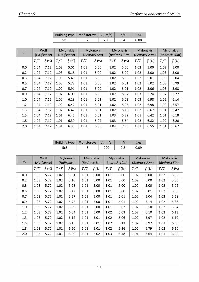
Chapter 5 Performed analysis and results
9 6
Building type # of storeys VS [m/s] h/r 1/
5x5 2 200 0.4 0.08
Wolf
(Halfspace) Mylonakis (Halfspace)
Mylonakis (Bedrock 5m)
Mylonakis (Bedrock 10m)
Mylonakis (Bedrock 20m)
Mylonakis (Bedrock 50m)
(%) (%) (%) (%) (%) (%)
0.0 1.04 7.12 1.03 5.01 1.01 5.00 1.02 5.00 1.02 5.00 1.02 5.00
0.2 1.04 7.12 1.03 5.18 1.01 5.00 1.02 5.00 1.02 5.00 1.03 5.00
0.3 1.04 7.12 1.03 5.49 1.01 5.00 1.02 5.00 1.02 5.01 1.03 5.04
0.5 1.04 7.12 1.03 5.72 1.01 5.00 1.02 5.01 1.02 5.02 1.03 5.99
0.7 1.04 7.12 1.02 5.91 1.01 5.00 1.02 5.01 1.02 5.06 1.03 5.98
0.9 1.04 7.12 1.02 6.09 1.01 5.00 1.02 5.02 1.03 5.24 1.02 6.22
1.0 1.04 7.12 1.02 6.28 1.01 5.01 1.02 5.03 1.03 6.98 1.02 6.14
1.2 1.04 7.12 1.02 6.42 1.01 5.01 1.02 5.06 1.02 6.98 1.02 6.57
1.3 1.04 7.12 1.02 6.47 1.01 5.01 1.02 5.10 1.02 6.67 1.01 6.42
1.5 1.04 7.12 1.01 6.45 1.01 5.01 1.03 5.22 1.01 6.42 1.01 6.18
1.8 1.04 7.12 1.01 6.39 1.01 5.02 1.03 5.64 1.02 6.82 1.02 6.20
2.0 1.04 7.12 1.01 6.33 1.01 5.03 1.04 7.66 1.01 6.55 1.01 6.67
Building type # of storeys VS [m/s] h/r 1/
5x5 5 200 0.8 0.09
Wolf
(Halfspace) Mylonakis (Halfspace)
Mylonakis (Bedrock 5m)
Mylonakis (Bedrock 10m)
Mylonakis (Bedrock 20m)
Mylonakis (Bedrock 50m)
(%) (%) (%) (%) (%) (%)
0.0 1.03 5.72 1.02 5.01 1.01 5.00 1.01 5.00 1.02 5.00 1.02 5.00
0.2 1.03 5.72 1.02 5.10 1.01 5.00 1.01 5.00 1.02 5.00 1.02 5.00
0.3 1.03 5.72 1.02 5.28 1.01 5.00 1.01 5.00 1.02 5.00 1.02 5.02
0.5 1.03 5.72 1.02 5.42 1.01 5.00 1.01 5.00 1.02 5.01 1.02 5.55
0.7 1.03 5.72 1.02 5.57 1.01 5.00 1.01 5.01 1.02 5.04 1.02 5.58
0.9 1.03 5.72 1.02 5.72 1.01 5.00 1.01 5.01 1.02 5.14 1.02 5.83
1.0 1.03 5.72 1.02 5.89 1.01 5.00 1.01 5.02 1.02 6.10 1.02 5.84
1.2 1.03 5.72 1.02 6.04 1.01 5.00 1.02 5.03 1.02 6.10 1.02 6.13
1.3 1.03 5.72 1.02 6.14 1.01 5.01 1.02 5.06 1.02 5.97 1.02 6.10
1.5 1.03 5.72 1.02 6.18 1.01 5.01 1.02 5.13 1.02 5.97 1.01 6.03
1.8 1.03 5.72 1.01 6.20 1.01 5.01 1.02 5.36 1.02 6.79 1.02 6.10
2.0 1.03 5.72 1.01 6.20 1.01 5.02 1.03 6.48 1.01 6.64 1.01 6.39

Chapter 5 Performed analysis and results
9 7
Building type # of storeys VS [m/s] h/r 1/
5x5 10 200 1.7 0.14
Wolf
(Halfspace) Mylonakis (Halfspace)
Mylonakis (Bedrock 5m)
Mylonakis (Bedrock 10m)
Mylonakis (Bedrock 20m)
Mylonakis (Bedrock 50m)
(%) (%) (%) (%) (%) (%)
0.0 1.06 5.66 1.04 5.01 1.02 5.00 1.03 5.00 1.03 5.00 1.04 5.00
0.2 1.06 5.66 1.04 5.09 1.02 5.00 1.03 5.00 1.03 5.00 1.04 5.00
0.3 1.06 5.66 1.04 5.26 1.02 5.00 1.03 5.00 1.03 5.01 1.04 5.03
0.5 1.06 5.66 1.04 5.45 1.02 5.00 1.03 5.00 1.04 5.02 1.04 5.48
0.7 1.06 5.66 1.04 5.70 1.02 5.00 1.03 5.01 1.04 5.04 1.04 5.61
0.9 1.06 5.66 1.04 6.01 1.02 5.00 1.03 5.02 1.04 5.14 1.04 6.19
1.0 1.06 5.66 1.04 6.37 1.02 5.00 1.03 5.03 1.04 5.97 1.04 6.38
1.2 1.06 5.66 1.04 6.72 1.02 5.01 1.03 5.04 1.04 6.01 1.04 6.79
1.3 1.06 5.66 1.04 7.02 1.02 5.01 1.03 5.07 1.04 6.01 1.04 6.94
1.5 1.06 5.66 1.04 7.24 1.02 5.01 1.03 5.13 1.05 6.44 1.04 7.07
1.8 1.06 5.66 1.03 7.41 1.02 5.02 1.04 5.35 1.05 8.96 1.04 7.32
2.0 1.06 5.66 1.03 7.51 1.02 5.02 1.04 6.31 1.03 8.90 1.03 7.70
Building type # of storeys VS [m/s] h/r 1/
5x5 20 200 3.4 0.23
Wolf
(Halfspace) Mylonakis (Halfspace)
Mylonakis (Bedrock 5m)
Mylonakis (Bedrock 10m)
Mylonakis (Bedrock 20m)
Mylonakis (Bedrock 50m)
(%) (%) (%) (%) (%) (%)
0.0 1.21 6.00 1.14 5.01 1.06 5.00 1.09 5.00 1.12 5.00 1.13 5.00
0.2 1.21 6.00 1.14 5.09 1.06 5.00 1.09 5.00 1.12 5.00 1.13 5.01
0.3 1.21 6.00 1.14 5.33 1.06 5.00 1.09 5.01 1.12 5.02 1.14 5.04
0.5 1.21 6.00 1.14 5.76 1.06 5.00 1.09 5.01 1.12 5.04 1.14 5.51
0.7 1.21 6.00 1.15 6.45 1.06 5.01 1.09 5.02 1.13 5.09 1.16 6.02
0.9 1.21 6.00 1.15 7.39 1.06 5.01 1.10 5.04 1.14 5.22 1.15 7.92
1.0 1.21 6.00 1.15 8.51 1.06 5.01 1.10 5.06 1.14 6.05 1.15 8.77
1.2 1.21 6.00 1.15 9.70 1.06 5.02 1.10 5.09 1.15 6.24 1.15 9.79
1.3 1.21 6.00 1.15 10.82 1.06 5.02 1.10 5.14 1.17 6.63 1.15 10.60
1.5 1.21 6.00 1.14 11.80 1.06 5.03 1.11 5.23 1.20 8.44 1.14 11.47
1.8 1.21 6.00 1.14 12.61 1.06 5.04 1.12 5.47 1.23 17.24 1.14 12.51
2.0 1.21 6.00 1.13 13.23 1.06 5.05 1.12 6.43 1.16 18.54 1.13 13.52

Chapter 5 Performed analysis and results
9 8
Building type # of storeys VS [m/s] h/r 1/
5x5 2 320 0.4 0.05
Wolf
(Halfspace) Mylonakis (Halfspace)
Mylonakis (Bedrock 5m)
Mylonakis (Bedrock 10m)
Mylonakis (Bedrock 20m)
Mylonakis (Bedrock 50m)
(%) (%) (%) (%) (%) (%)
0.0 1.01 5.55 1.01 5.00 1.00 5.00 1.01 5.00 1.01 5.00 1.01 5.00
0.1 1.01 5.55 1.01 5.04 1.00 5.00 1.01 5.00 1.01 5.00 1.01 5.00
0.3 1.01 5.55 1.01 5.20 1.00 5.00 1.01 5.00 1.01 5.00 1.01 5.02
0.5 1.01 5.55 1.01 5.31 1.00 5.00 1.01 5.00 1.01 5.01 1.01 5.40
0.8 1.01 5.55 1.01 5.40 1.00 5.00 1.01 5.01 1.01 5.05 1.01 5.51
1.0 1.01 5.55 1.01 5.50 1.00 5.00 1.01 5.01 1.01 5.71 1.01 5.45
1.3 1.01 5.55 1.01 5.57 1.00 5.00 1.01 5.02 1.01 5.78 1.01 5.63
1.5 1.01 5.55 1.01 5.58 1.00 5.00 1.01 5.05 1.01 5.62 1.01 5.53
1.7 1.01 5.55 1.01 5.56 1.00 5.01 1.01 5.15 1.01 5.60 1.01 5.45
2.0 1.01 5.55 1.00 5.53 1.00 5.01 1.01 6.05 1.00 5.62 1.01 5.66
Building type # of storeys VS [m/s] h/r 1/
5x5 5 320 0.8 0.06
Wolf
(Halfspace) Mylonakis (Halfspace)
Mylonakis (Bedrock 5m)
Mylonakis (Bedrock 10m)
Mylonakis (Bedrock 20m)
Mylonakis (Bedrock 50m)
(%) (%) (%) (%) (%) (%)
0.0 1.01 5.19 1.01 5.00 1.00 5.00 1.01 5.00 1.01 5.00 1.01 5.00
0.1 1.01 5.19 1.01 5.02 1.00 5.00 1.01 5.00 1.01 5.00 1.01 5.00
0.3 1.01 5.19 1.01 5.11 1.00 5.00 1.01 5.00 1.01 5.00 1.01 5.01
0.5 1.01 5.19 1.01 5.19 1.00 5.00 1.01 5.00 1.01 5.01 1.01 5.22
0.8 1.01 5.19 1.01 5.26 1.00 5.00 1.01 5.00 1.01 5.03 1.01 5.33
1.0 1.01 5.19 1.01 5.34 1.00 5.00 1.01 5.01 1.01 5.39 1.01 5.33
1.3 1.01 5.19 1.01 5.42 1.00 5.00 1.01 5.01 1.01 5.44 1.01 5.45
1.5 1.01 5.19 1.01 5.46 1.00 5.00 1.01 5.03 1.01 5.37 1.01 5.43
1.7 1.01 5.19 1.01 5.47 1.00 5.00 1.01 5.09 1.01 5.53 1.01 5.41
2.0 1.01 5.19 1.00 5.47 1.00 5.01 1.01 5.58 1.00 5.65 1.01 5.55
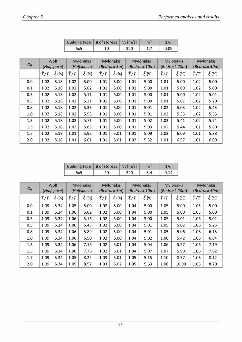
Chapter 5 Performed analysis and results
9 9
Building type # of storeys VS [m/s] h/r 1/
5x5 10 320 1.7 0.09
Wolf
(Halfspace) Mylonakis (Halfspace)
Mylonakis (Bedrock 5m)
Mylonakis (Bedrock 10m)
Mylonakis (Bedrock 20m)
Mylonakis (Bedrock 50m)
(%) (%) (%) (%) (%) (%)
0.0 1.02 5.18 1.02 5.00 1.01 5.00 1.01 5.00 1.01 5.00 1.02 5.00
0.1 1.02 5.18 1.02 5.02 1.01 5.00 1.01 5.00 1.01 5.00 1.02 5.00
0.3 1.02 5.18 1.02 5.11 1.01 5.00 1.01 5.00 1.01 5.00 1.02 5.01
0.5 1.02 5.18 1.02 5.21 1.01 5.00 1.01 5.00 1.01 5.01 1.02 5.20
0.8 1.02 5.18 1.02 5.35 1.01 5.00 1.01 5.01 1.02 5.03 1.02 5.45
1.0 1.02 5.18 1.02 5.53 1.01 5.00 1.01 5.01 1.02 5.35 1.02 5.55
1.3 1.02 5.18 1.02 5.71 1.01 5.00 1.01 5.02 1.02 5.41 1.02 5.74
1.5 1.02 5.18 1.02 5.85 1.01 5.00 1.01 5.03 1.02 5.44 1.01 5.80
1.7 1.02 5.18 1.01 5.95 1.01 5.01 1.01 5.09 1.02 6.09 1.01 5.88
2.0 1.02 5.18 1.01 6.01 1.01 5.01 1.02 5.52 1.01 6.57 1.01 6.09
Building type # of storeys VS [m/s] h/r 1/
5x5 20 320 3.4 0.14
Wolf
(Halfspace) Mylonakis (Halfspace)
Mylonakis (Bedrock 5m)
Mylonakis (Bedrock 10m)
Mylonakis (Bedrock 20m)
Mylonakis (Bedrock 50m)
(%) (%) (%) (%) (%) (%)
0.0 1.09 5.34 1.05 5.00 1.02 5.00 1.04 5.00 1.05 5.00 1.05 5.00
0.1 1.09 5.34 1.06 5.02 1.02 5.00 1.04 5.00 1.05 5.00 1.05 5.00
0.3 1.09 5.34 1.06 5.16 1.02 5.00 1.04 5.00 1.05 5.01 1.06 5.02
0.5 1.09 5.34 1.06 5.43 1.02 5.00 1.04 5.01 1.05 5.02 1.06 5.25
0.8 1.09 5.34 1.06 5.89 1.02 5.00 1.04 5.01 1.05 5.06 1.06 6.15
1.0 1.09 5.34 1.06 6.50 1.02 5.00 1.04 5.02 1.06 5.42 1.06 6.64
1.3 1.09 5.34 1.06 7.16 1.02 5.01 1.04 5.04 1.06 5.57 1.06 7.19
1.5 1.09 5.34 1.06 7.76 1.02 5.01 1.04 5.07 1.07 5.90 1.06 7.62
1.7 1.09 5.34 1.05 8.22 1.03 5.01 1.05 5.15 1.10 8.57 1.06 8.12
2.0 1.09 5.34 1.05 8.57 1.03 5.02 1.05 5.63 1.06 10.90 1.05 8.70

Chapter 5 Performed analysis and results
1 0 0
Results for buildings 10x10
Building type # of storeys VS [m/s] h/r 1/
10x10 2 80 0.2 0.16
Wolf
(Halfspace) Mylonakis (Halfspace)
Mylonakis (Bedrock 5m)
Mylonakis (Bedrock 10m)
Mylonakis (Bedrock 20m)
Mylonakis (Bedrock 50m)
(%) (%) (%) (%) (%) (%)
0.0 1.21 44.16 1.18 5.38 1.04 5.00 1.07 5.00 1.10 5.00 1.14 5.01
0.5 1.21 44.16 1.17 9.61 1.04 5.00 1.07 5.01 1.11 5.03 1.16 5.20
1.0 1.21 44.16 1.14 11.97 1.04 5.01 1.07 5.03 1.12 5.14 1.18 15.59
1.4 1.21 44.16 1.11 12.43 1.04 5.01 1.08 5.06 1.14 5.60 1.13 14.99
1.9 1.21 44.16 1.10 12.62 1.05 5.02 1.08 5.14 1.26 12.38 1.07 11.91
2.0 1.21 44.16 1.10 12.77 1.05 5.02 1.08 5.16 1.27 19.72 1.07 11.31
Building type # of storeys VS [m/s] h/r 1/
10x10 5 80 0.4 0.20
Wolf
(Halfspace) Mylonakis (Halfspace)
Mylonakis (Bedrock 5m)
Mylonakis (Bedrock 10m)
Mylonakis (Bedrock 20m)
Mylonakis (Bedrock 50m)
0.0 1.14 19.96 1.12 5.24 1.03 5.00 1.05 5.00 1.07 5.00 1.09 5.00
0.5 1.14 19.96 1.11 7.91 1.03 5.00 1.05 5.01 1.07 5.02 1.11 5.14
1.0 1.14 19.96 1.09 9.49 1.03 5.00 1.05 5.02 1.08 5.09 1.12 11.51
1.4 1.14 19.96 1.08 10.02 1.03 5.01 1.05 5.04 1.09 5.38 1.09 11.76
1.9 1.14 19.96 1.07 10.34 1.03 5.01 1.05 5.09 1.16 9.83 1.05 10.11
2.0 1.14 19.96 1.07 10.45 1.03 5.01 1.05 5.10 1.16 14.41 1.05 9.74
Building type # of storeys VS [m/s] h/r 1/
10x10 10 80 0.8 0.31
Wolf
(Halfspace) Mylonakis (Halfspace)
Mylonakis (Bedrock 5m)
Mylonakis (Bedrock 10m)
Mylonakis (Bedrock 20m)
Mylonakis (Bedrock 50m)
(%) (%) (%) (%) (%) (%)
0.0 1.20 15.95 1.15 5.21 1.04 5.00 1.06 5.00 1.09 5.00 1.13 5.00
0.5 1.20 15.95 1.15 7.71 1.04 5.00 1.06 5.01 1.10 5.03 1.14 5.16
1.0 1.20 15.95 1.14 9.79 1.04 5.01 1.07 5.02 1.10 5.10 1.15 10.75
1.4 1.20 15.95 1.13 11.33 1.04 5.01 1.07 5.05 1.12 5.38 1.17 13.44
1.9 1.20 15.95 1.11 12.47 1.04 5.01 1.07 5.09 1.19 9.39 1.10 13.10
2.0 1.20 15.95 1.11 12.70 1.04 5.02 1.07 5.11 1.19 13.44 1.09 12.72
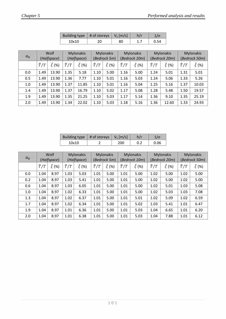
Chapter 5 Performed analysis and results
1 0 1
Building type # of storeys VS [m/s] h/r 1/
10x10 20 80 1.7 0.54
Wolf
(Halfspace) Mylonakis (Halfspace)
Mylonakis (Bedrock 5m)
Mylonakis (Bedrock 10m)
Mylonakis (Bedrock 20m)
Mylonakis (Bedrock 50m)
(%) (%) (%) (%) (%) (%)
0.0 1.49 13.90 1.35 5.18 1.10 5.00 1.16 5.00 1.24 5.01 1.31 5.01
0.5 1.49 13.90 1.36 7.77 1.10 5.01 1.16 5.03 1.24 5.06 1.33 5.26
1.0 1.49 13.90 1.37 11.85 1.10 5.01 1.16 5.04 1.25 5.16 1.37 10.03
1.4 1.49 13.90 1.37 16.79 1.10 5.02 1.17 5.08 1.28 5.48 1.50 19.57
1.9 1.49 13.90 1.35 21.25 1.10 5.03 1.17 5.14 1.36 9.10 1.35 25.19
2.0 1.49 13.90 1.34 22.02 1.10 5.03 1.18 5.16 1.36 12.60 1.33 24.93
Building type # of storeys VS [m/s] h/r 1/
10x10 2 200 0.2 0.06
Wolf
(Halfspace) Mylonakis (Halfspace)
Mylonakis (Bedrock 5m)
Mylonakis (Bedrock 10m)
Mylonakis (Bedrock 20m)
Mylonakis (Bedrock 50m)
(%) (%) (%) (%) (%) (%)
0.0 1.04 8.97 1.03 5.03 1.01 5.00 1.01 5.00 1.02 5.00 1.02 5.00
0.2 1.04 8.97 1.03 5.41 1.01 5.00 1.01 5.00 1.02 5.00 1.02 5.00
0.6 1.04 8.97 1.03 6.05 1.01 5.00 1.01 5.00 1.02 5.01 1.03 5.08
1.0 1.04 8.97 1.02 6.33 1.01 5.00 1.01 5.00 1.02 5.03 1.03 7.08
1.3 1.04 8.97 1.02 6.37 1.01 5.00 1.01 5.01 1.02 5.09 1.02 6.59
1.7 1.04 8.97 1.02 6.34 1.01 5.00 1.01 5.02 1.03 5.41 1.01 6.47
1.9 1.04 8.97 1.01 6.36 1.01 5.00 1.01 5.03 1.04 6.65 1.01 6.20
2.0 1.04 8.97 1.01 6.38 1.01 5.00 1.01 5.03 1.04 7.88 1.01 6.12
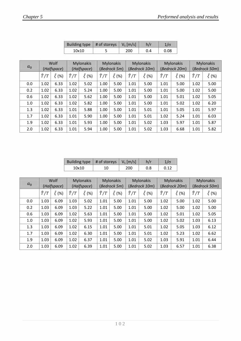
Chapter 5 Performed analysis and results
1 0 2
Building type # of storeys VS [m/s] h/r 1/
10x10 5 200 0.4 0.08
Wolf
(Halfspace) Mylonakis (Halfspace)
Mylonakis (Bedrock 5m)
Mylonakis (Bedrock 10m)
Mylonakis (Bedrock 20m)
Mylonakis (Bedrock 50m)
(%) (%) (%) (%) (%) (%)
0.0 1.02 6.33 1.02 5.02 1.00 5.00 1.01 5.00 1.01 5.00 1.02 5.00
0.2 1.02 6.33 1.02 5.24 1.00 5.00 1.01 5.00 1.01 5.00 1.02 5.00
0.6 1.02 6.33 1.02 5.62 1.00 5.00 1.01 5.00 1.01 5.01 1.02 5.05
1.0 1.02 6.33 1.02 5.82 1.00 5.00 1.01 5.00 1.01 5.02 1.02 6.20
1.3 1.02 6.33 1.01 5.88 1.00 5.00 1.01 5.01 1.01 5.05 1.01 5.97
1.7 1.02 6.33 1.01 5.90 1.00 5.00 1.01 5.01 1.02 5.24 1.01 6.03
1.9 1.02 6.33 1.01 5.93 1.00 5.00 1.01 5.02 1.03 5.97 1.01 5.87
2.0 1.02 6.33 1.01 5.94 1.00 5.00 1.01 5.02 1.03 6.68 1.01 5.82
Building type # of storeys VS [m/s] h/r 1/
10x10 10 200 0.8 0.12
Wolf
(Halfspace) Mylonakis (Halfspace)
Mylonakis (Bedrock 5m)
Mylonakis (Bedrock 10m)
Mylonakis (Bedrock 20m)
Mylonakis (Bedrock 50m)
(%) (%) (%) (%) (%) (%)
0.0 1.03 6.09 1.03 5.02 1.01 5.00 1.01 5.00 1.02 5.00 1.02 5.00
0.2 1.03 6.09 1.03 5.22 1.01 5.00 1.01 5.00 1.02 5.00 1.02 5.00
0.6 1.03 6.09 1.02 5.63 1.01 5.00 1.01 5.00 1.02 5.01 1.02 5.05
1.0 1.03 6.09 1.02 5.93 1.01 5.00 1.01 5.00 1.02 5.02 1.03 6.13
1.3 1.03 6.09 1.02 6.15 1.01 5.00 1.01 5.01 1.02 5.05 1.03 6.12
1.7 1.03 6.09 1.02 6.30 1.01 5.00 1.01 5.01 1.02 5.23 1.02 6.62
1.9 1.03 6.09 1.02 6.37 1.01 5.00 1.01 5.02 1.03 5.91 1.01 6.44
2.0 1.03 6.09 1.02 6.39 1.01 5.00 1.01 5.02 1.03 6.57 1.01 6.38
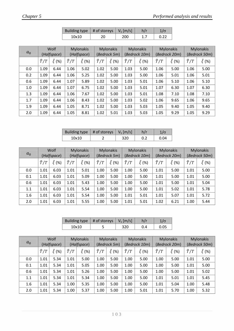
Chapter 5 Performed analysis and results
1 0 3
Building type # of storeys VS [m/s] h/r 1/
10x10 20 200 1.7 0.22
Wolf
(Halfspace) Mylonakis (Halfspace)
Mylonakis (Bedrock 5m)
Mylonakis (Bedrock 10m)
Mylonakis (Bedrock 20m)
Mylonakis (Bedrock 50m)
(%) (%) (%) (%) (%) (%)
0.0 1.09 6.44 1.06 5.02 1.02 5.00 1.03 5.00 1.06 5.00 1.06 5.00
0.2 1.09 6.44 1.06 5.25 1.02 5.00 1.03 5.00 1.06 5.01 1.06 5.01
0.6 1.09 6.44 1.07 5.89 1.02 5.00 1.03 5.01 1.06 5.10 1.06 5.10
1.0 1.09 6.44 1.07 6.75 1.02 5.00 1.03 5.01 1.07 6.30 1.07 6.30
1.3 1.09 6.44 1.06 7.67 1.02 5.00 1.03 5.01 1.08 7.10 1.08 7.10
1.7 1.09 6.44 1.06 8.43 1.02 5.00 1.03 5.02 1.06 9.65 1.06 9.65
1.9 1.09 6.44 1.05 8.71 1.02 5.00 1.03 5.03 1.05 9.40 1.05 9.40
2.0 1.09 6.44 1.05 8.81 1.02 5.01 1.03 5.03 1.05 9.29 1.05 9.29
Building type # of storeys VS [m/s] h/r 1/
10x10 2 320 0.2 0.04
Wolf
(Halfspace) Mylonakis (Halfspace)
Mylonakis (Bedrock 5m)
Mylonakis (Bedrock 10m)
Mylonakis (Bedrock 20m)
Mylonakis (Bedrock 50m)
(%) (%) (%) (%) (%) (%)
0.0 1.01 6.03 1.01 5.01 1.00 5.00 1.00 5.00 1.01 5.00 1.01 5.00
0.1 1.01 6.03 1.01 5.09 1.00 5.00 1.00 5.00 1.01 5.00 1.01 5.00
0.6 1.01 6.03 1.01 5.43 1.00 5.00 1.00 5.00 1.01 5.00 1.01 5.04
1.1 1.01 6.03 1.01 5.54 1.00 5.00 1.00 5.00 1.01 5.02 1.01 5.78
1.6 1.01 6.03 1.01 5.54 1.00 5.00 1.01 5.01 1.01 5.07 1.01 5.72
2.0 1.01 6.03 1.01 5.55 1.00 5.00 1.01 5.01 1.02 6.21 1.00 5.44
Building type # of storeys VS [m/s] h/r 1/
10x10 5 320 0.4 0.05
Wolf
(Halfspace) Mylonakis (Halfspace)
Mylonakis (Bedrock 5m)
Mylonakis (Bedrock 10m)
Mylonakis (Bedrock 20m)
Mylonakis (Bedrock 50m)
(%) (%) (%) (%) (%) (%)
0.0 1.01 5.34 1.01 5.00 1.00 5.00 1.00 5.00 1.00 5.00 1.01 5.00
0.1 1.01 5.34 1.01 5.05 1.00 5.00 1.00 5.00 1.00 5.00 1.01 5.00
0.6 1.01 5.34 1.01 5.26 1.00 5.00 1.00 5.00 1.00 5.00 1.01 5.02
1.1 1.01 5.34 1.01 5.34 1.00 5.00 1.00 5.00 1.01 5.01 1.01 5.45
1.6 1.01 5.34 1.00 5.35 1.00 5.00 1.00 5.00 1.01 5.04 1.00 5.48
2.0 1.01 5.34 1.00 5.37 1.00 5.00 1.00 5.01 1.01 5.70 1.00 5.32
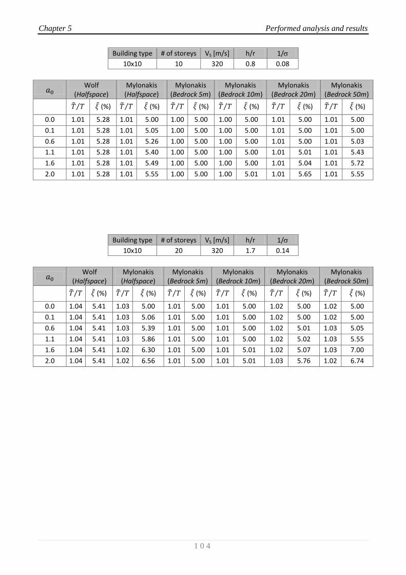
Chapter 5 Performed analysis and results
1 0 4
Building type # of storeys VS [m/s] h/r 1/
10x10 10 320 0.8 0.08
Wolf
(Halfspace) Mylonakis (Halfspace)
Mylonakis (Bedrock 5m)
Mylonakis (Bedrock 10m)
Mylonakis (Bedrock 20m)
Mylonakis (Bedrock 50m)
(%) (%) (%) (%) (%) (%)
0.0 1.01 5.28 1.01 5.00 1.00 5.00 1.00 5.00 1.01 5.00 1.01 5.00
0.1 1.01 5.28 1.01 5.05 1.00 5.00 1.00 5.00 1.01 5.00 1.01 5.00
0.6 1.01 5.28 1.01 5.26 1.00 5.00 1.00 5.00 1.01 5.00 1.01 5.03
1.1 1.01 5.28 1.01 5.40 1.00 5.00 1.00 5.00 1.01 5.01 1.01 5.43
1.6 1.01 5.28 1.01 5.49 1.00 5.00 1.00 5.00 1.01 5.04 1.01 5.72
2.0 1.01 5.28 1.01 5.55 1.00 5.00 1.00 5.01 1.01 5.65 1.01 5.55
Building type # of storeys VS [m/s] h/r 1/
10x10 20 320 1.7 0.14
Wolf
(Halfspace) Mylonakis (Halfspace)
Mylonakis (Bedrock 5m)
Mylonakis (Bedrock 10m)
Mylonakis (Bedrock 20m)
Mylonakis (Bedrock 50m)
(%) (%) (%) (%) (%) (%)
0.0 1.04 5.41 1.03 5.00 1.01 5.00 1.01 5.00 1.02 5.00 1.02 5.00
0.1 1.04 5.41 1.03 5.06 1.01 5.00 1.01 5.00 1.02 5.00 1.02 5.00
0.6 1.04 5.41 1.03 5.39 1.01 5.00 1.01 5.00 1.02 5.01 1.03 5.05
1.1 1.04 5.41 1.03 5.86 1.01 5.00 1.01 5.00 1.02 5.02 1.03 5.55
1.6 1.04 5.41 1.02 6.30 1.01 5.00 1.01 5.01 1.02 5.07 1.03 7.00
2.0 1.04 5.41 1.02 6.56 1.01 5.00 1.01 5.01 1.03 5.76 1.02 6.74

Chapter 5 Performed analysis and results
1 0 5
All the above solutions presented in tables can be directly used for pre-design purpose; in
addition, results can be summarized in ready-to-use charts, which allow the practitioners to deal
with SSI in an immediate manner.
Such charts are presented hereinafter for the case of homogeneous halfspace and for the
different bedrock positions considered in the analyses, in form of
and as function of ;
comparison between Wolf’s and Mylonakis’ solutions is also presented.
Results for buildings 2x2
Fig. 5.5-8: Dimensionless chart: modified period for 2x2 buildings - VS = 80 m/s
1.00
2.00
3.00
4.00
5.00
0.05 0.20 0.35 0.50 0.65 0.80
T/T
1/
Building 2x2Halfspace
Vs = 80 m/s
Mylonakis
Wolf
1.00
2.00
3.00
4.00
5.00
0.05 0.20 0.35 0.50 0.65 0.80
T/T
1/
Building 2x2Bedrock 5mVs = 80 m/s
Mylonakis
Wolf
1.00
2.00
3.00
4.00
5.00
0.05 0.20 0.35 0.50 0.65 0.80
T/T
1/
Building 2x2Bedrock 10mVs = 80 m/s
Mylonakis
Wolf
1.00
2.00
3.00
4.00
5.00
0.05 0.20 0.35 0.50 0.65 0.80
T/T
1/
Building 2x2Bedrock 20mVs = 80 m/s
Mylonakis
Wolf
1.00
2.00
3.00
4.00
5.00
0.05 0.20 0.35 0.50 0.65 0.80
T/T
1/
Building 2x2Bedrock 50mVs = 80 m/s
Mylonakis
Wolf
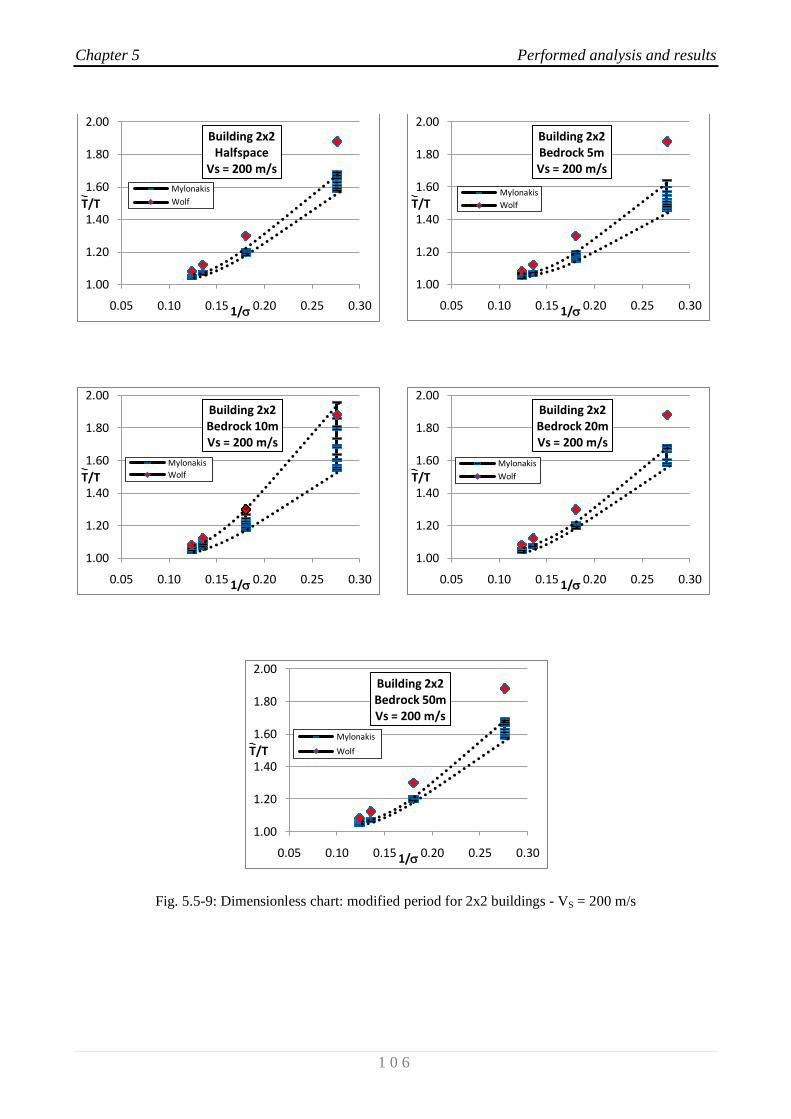
Chapter 5 Performed analysis and results
1 0 6
Fig. 5.5-9: Dimensionless chart: modified period for 2x2 buildings - VS = 200 m/s
1.00
1.20
1.40
1.60
1.80
2.00
0.05 0.10 0.15 0.20 0.25 0.30
T/T
1/
Building 2x2Halfspace
Vs = 200 m/s
Mylonakis
Wolf
1.00
1.20
1.40
1.60
1.80
2.00
0.05 0.10 0.15 0.20 0.25 0.30
T/T
1/
Building 2x2Bedrock 5mVs = 200 m/s
Mylonakis
Wolf
1.00
1.20
1.40
1.60
1.80
2.00
0.05 0.10 0.15 0.20 0.25 0.30
T/T
1/
Building 2x2Bedrock 10mVs = 200 m/s
Mylonakis
Wolf
1.00
1.20
1.40
1.60
1.80
2.00
0.05 0.10 0.15 0.20 0.25 0.30
T/T
1/
Building 2x2Bedrock 20mVs = 200 m/s
Mylonakis
Wolf
1.00
1.20
1.40
1.60
1.80
2.00
0.05 0.10 0.15 0.20 0.25 0.30
T/T
1/
Building 2x2Bedrock 50mVs = 200 m/s
Mylonakis
Wolf

Chapter 5 Performed analysis and results
1 0 7
Fig. 5.5-10: Dimensionless chart: modified period for 2x2 buildings - VS = 320 m/s
1.00
1.10
1.20
1.30
1.40
1.50
0.05 0.10 0.15 0.20
T/T
1/
Building 2x2Halfspace
Vs = 320 m/s
Mylonakis
Wolf
1.00
1.10
1.20
1.30
1.40
1.50
0.05 0.10 0.15 0.20
T/T
1/
Building 2x2Bedrock 5mVs = 320 m/s
Mylonakis
Wolf
1.00
1.10
1.20
1.30
1.40
1.50
0.05 0.10 0.15 0.20
T/T
1/
Building 2x2Bedrock 10mVs = 320 m/s
Mylonakis
Wolf
1.00
1.10
1.20
1.30
1.40
1.50
0.05 0.10 0.15 0.20
T/T
1/
Building 2x2Bedrock 20mVs = 320 m/s
Mylonakis
Wolf
1.00
1.10
1.20
1.30
1.40
1.50
0.05 0.10 0.15 0.20
T/T
1/
Building 2x2Bedrock 50mVs = 320 m/s
Mylonakis
Wolf
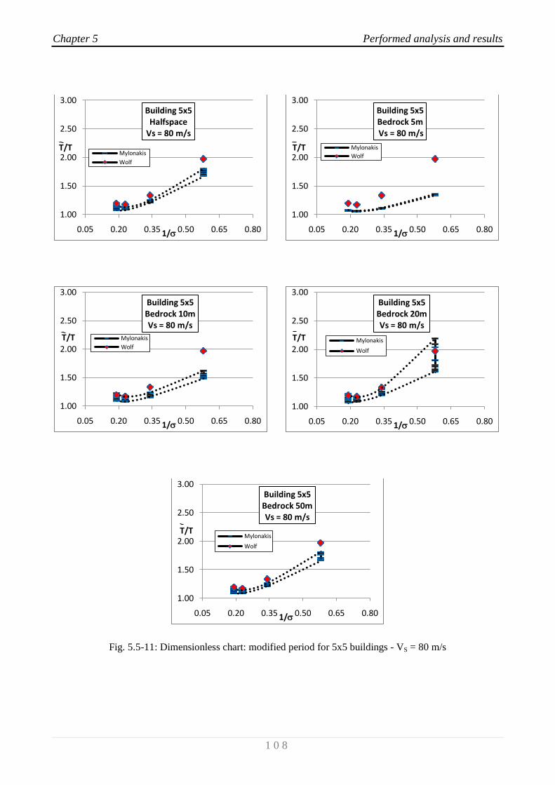
Chapter 5 Performed analysis and results
1 0 8
Fig. 5.5-11: Dimensionless chart: modified period for 5x5 buildings - VS = 80 m/s
1.00
1.50
2.00
2.50
3.00
0.05 0.20 0.35 0.50 0.65 0.80
T/T
1/
Building 5x5Halfspace
Vs = 80 m/s
Mylonakis
Wolf
1.00
1.50
2.00
2.50
3.00
0.05 0.20 0.35 0.50 0.65 0.80
T/T
1/
Building 5x5Bedrock 5mVs = 80 m/s
Mylonakis
Wolf
1.00
1.50
2.00
2.50
3.00
0.05 0.20 0.35 0.50 0.65 0.80
T/T
1/
Building 5x5Bedrock 10mVs = 80 m/s
Mylonakis
Wolf
1.00
1.50
2.00
2.50
3.00
0.05 0.20 0.35 0.50 0.65 0.80
T/T
1/
Building 5x5Bedrock 20mVs = 80 m/s
Mylonakis
Wolf
1.00
1.50
2.00
2.50
3.00
0.05 0.20 0.35 0.50 0.65 0.80
T/T
1/
Building 5x5Bedrock 50mVs = 80 m/s
Mylonakis
Wolf
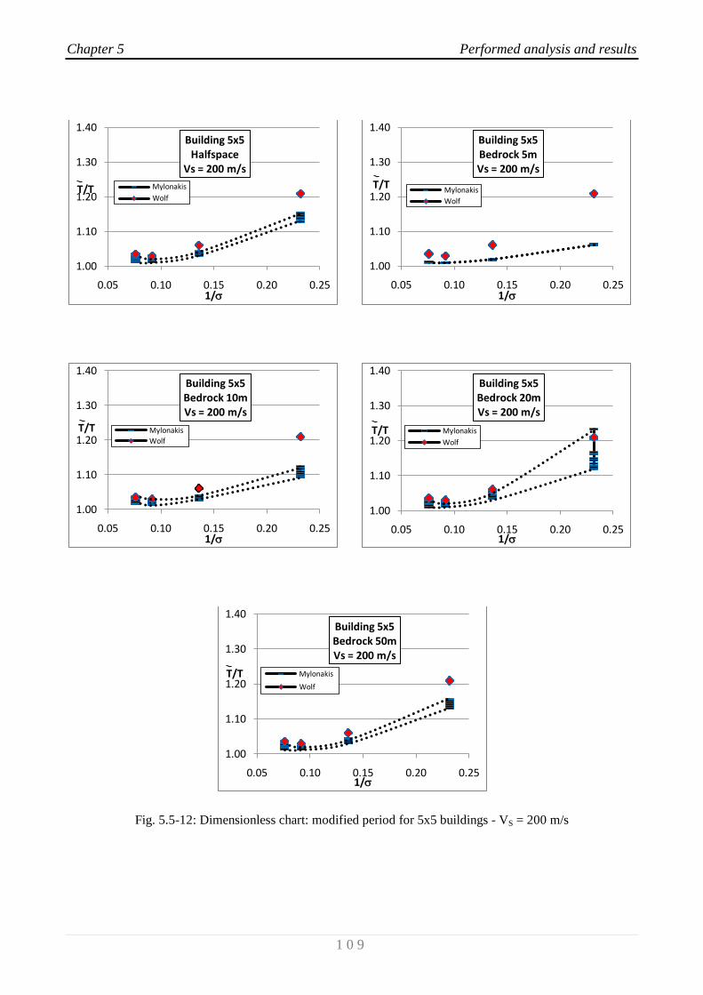
Chapter 5 Performed analysis and results
1 0 9
Fig. 5.5-12: Dimensionless chart: modified period for 5x5 buildings - VS = 200 m/s
1.00
1.10
1.20
1.30
1.40
0.05 0.10 0.15 0.20 0.25
T/T
1/
Building 5x5Halfspace
Vs = 200 m/s
Mylonakis
Wolf
1.00
1.10
1.20
1.30
1.40
0.05 0.10 0.15 0.20 0.25
T/T
1/
Building 5x5Bedrock 5mVs = 200 m/s
Mylonakis
Wolf
1.00
1.10
1.20
1.30
1.40
0.05 0.10 0.15 0.20 0.25
T/T
1/
Building 5x5Bedrock 10mVs = 200 m/s
Mylonakis
Wolf
1.00
1.10
1.20
1.30
1.40
0.05 0.10 0.15 0.20 0.25
T/T
1/
Building 5x5Bedrock 20mVs = 200 m/s
Mylonakis
Wolf
1.00
1.10
1.20
1.30
1.40
0.05 0.10 0.15 0.20 0.25
T/T
1/
Building 5x5Bedrock 50mVs = 200 m/s
Mylonakis
Wolf
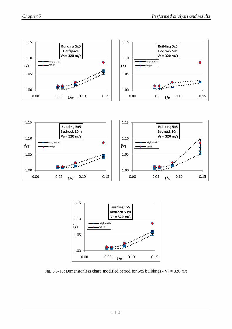
Chapter 5 Performed analysis and results
1 1 0
Fig. 5.5-13: Dimensionless chart: modified period for 5x5 buildings - VS = 320 m/s
1.00
1.05
1.10
1.15
0.00 0.05 0.10 0.15
T/T
1/
Building 5x5Halfspace
Vs = 320 m/s
Mylonakis
Wolf
1.00
1.05
1.10
1.15
0.00 0.05 0.10 0.15
T/T
1/
Building 5x5Bedrock 5mVs = 320 m/s
Mylonakis
Wolf
1.00
1.05
1.10
1.15
0.00 0.05 0.10 0.15
T/T
1/
Building 5x5Bedrock 10mVs = 320 m/s
Mylonakis
Wolf
1.00
1.05
1.10
1.15
0.00 0.05 0.10 0.15
T/T
1/
Building 5x5Bedrock 20mVs = 320 m/s
Mylonakis
Wolf
1.00
1.05
1.10
1.15
0.00 0.05 0.10 0.15
T/T
1/
Building 5x5Bedrock 50mVs = 320 m/s
Mylonakis
Wolf
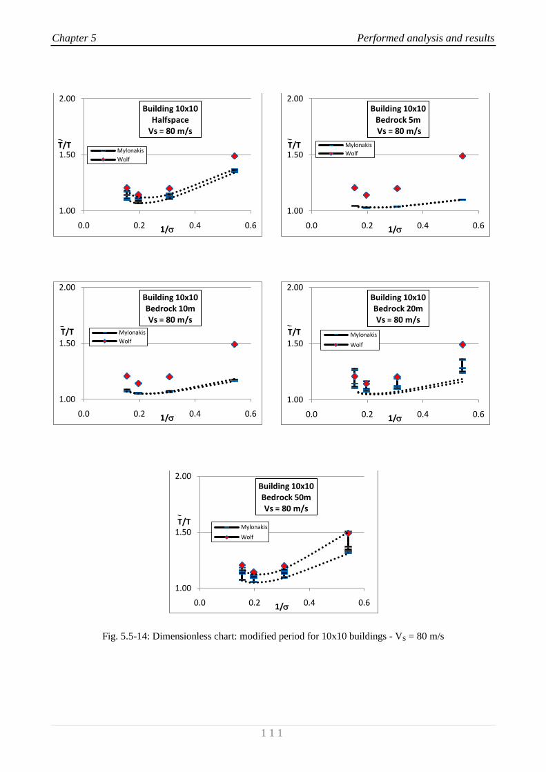
Chapter 5 Performed analysis and results
1 1 1
Fig. 5.5-14: Dimensionless chart: modified period for 10x10 buildings - VS = 80 m/s
1.00
1.50
2.00
0.0 0.2 0.4 0.6
T/T
1/
Building 10x10Halfspace
Vs = 80 m/s
Mylonakis
Wolf
1.00
1.50
2.00
0.0 0.2 0.4 0.6
T/T
1/
Building 10x10Bedrock 5mVs = 80 m/s
Mylonakis
Wolf
1.00
1.50
2.00
0.0 0.2 0.4 0.6
T/T
1/
Building 10x10Bedrock 10mVs = 80 m/s
Mylonakis
Wolf
1.00
1.50
2.00
0.0 0.2 0.4 0.6
T/T
1/
Building 10x10Bedrock 20mVs = 80 m/s
Mylonakis
Wolf
1.00
1.50
2.00
0.0 0.2 0.4 0.6
T/T
1/
Building 10x10Bedrock 50mVs = 80 m/s
Mylonakis
Wolf

Chapter 5 Performed analysis and results
1 1 2
Fig. 5.5-15: Dimensionless chart: modified period for 10x10 buildings - VS = 200 m/s
1.00
1.07
1.14
1.21
1.28
1.35
0.05 0.10 0.15 0.20 0.25
T/T
1/
Building 10x10Halfspace
Vs = 200 m/s
Mylonakis
Wolf
1.00
1.07
1.14
1.21
1.28
1.35
0.05 0.10 0.15 0.20 0.25
T/T
1/
Building 10x10Bedrock 5mVs = 200 m/s
Mylonakis
Wolf
1.00
1.07
1.14
1.21
1.28
1.35
0.05 0.10 0.15 0.20 0.25
T/T
1/
Building 10x10Bedrock 10mVs = 200 m/s
Mylonakis
Wolf
1.00
1.07
1.14
1.21
1.28
1.35
0.05 0.10 0.15 0.20 0.25
T/T
1/
Building 10x10Bedrock 20mVs = 200 m/s
Mylonakis
Wolf
1.00
1.07
1.14
1.21
1.28
1.35
0.05 0.10 0.15 0.20 0.25
T/T
1/
Building 10x10Bedrock 50mVs = 200 m/s
Mylonakis
Wolf
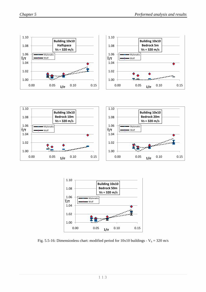
Chapter 5 Performed analysis and results
1 1 3
Fig. 5.5-16: Dimensionless chart: modified period for 10x10 buildings - VS = 320 m/s
1.00
1.02
1.04
1.06
1.08
1.10
0.00 0.05 0.10 0.15
T/T
1/
Building 10x10Halfspace
Vs = 320 m/s
Mylonakis
Wolf
1.00
1.02
1.04
1.06
1.08
1.10
0.00 0.05 0.10 0.15
T/T
1/
Building 10x10Bedrock 5mVs = 320 m/s
Mylonakis
Wolf
1.00
1.02
1.04
1.06
1.08
1.10
0.00 0.05 0.10 0.15
T/T
1/
Building 10x10Bedrock 10mVs = 320 m/s
Mylonakis
Wolf
1.00
1.02
1.04
1.06
1.08
1.10
0.00 0.05 0.10 0.15
T/T
1/
Building 10x10Bedrock 20mVs = 320 m/s
Mylonakis
Wolf
1.00
1.02
1.04
1.06
1.08
1.10
0.00 0.05 0.10 0.15
T/T
1/
Building 10x10Bedrock 50mVs = 320 m/s
Mylonakis
Wolf

Chapter 5 Performed analysis and results
1 1 4
Fig. 5.5-17: Dimensionless chart: modified damping for 2x2 buildings - VS = 80 m/s
0%
20%
40%
60%
0.05 0.20 0.35 0.50 0.65 0.80
1/
Building 2x2Halfspace
Vs = 80 m/s
Mylonakis
Wolf
0%
20%
40%
60%
0.05 0.20 0.35 0.50 0.65 0.80
1/
Building 2x2Bedrock 5mVs = 80 m/s
Mylonakis
Wolf
0%
20%
40%
60%
0.05 0.20 0.35 0.50 0.65 0.80
1/
Building 2x2Bedrock 10mVs = 80 m/s
Mylonakis
Wolf
0%
20%
40%
60%
0.05 0.20 0.35 0.50 0.65 0.80
1/
Building 2x2Bedrock 20mVs = 80 m/s
Mylonakis
Wolf
0%
20%
40%
60%
0.05 0.20 0.35 0.50 0.65 0.80
1/
Building 2x2Bedrock 50mVs = 80 m/s
Mylonakis
Wolf
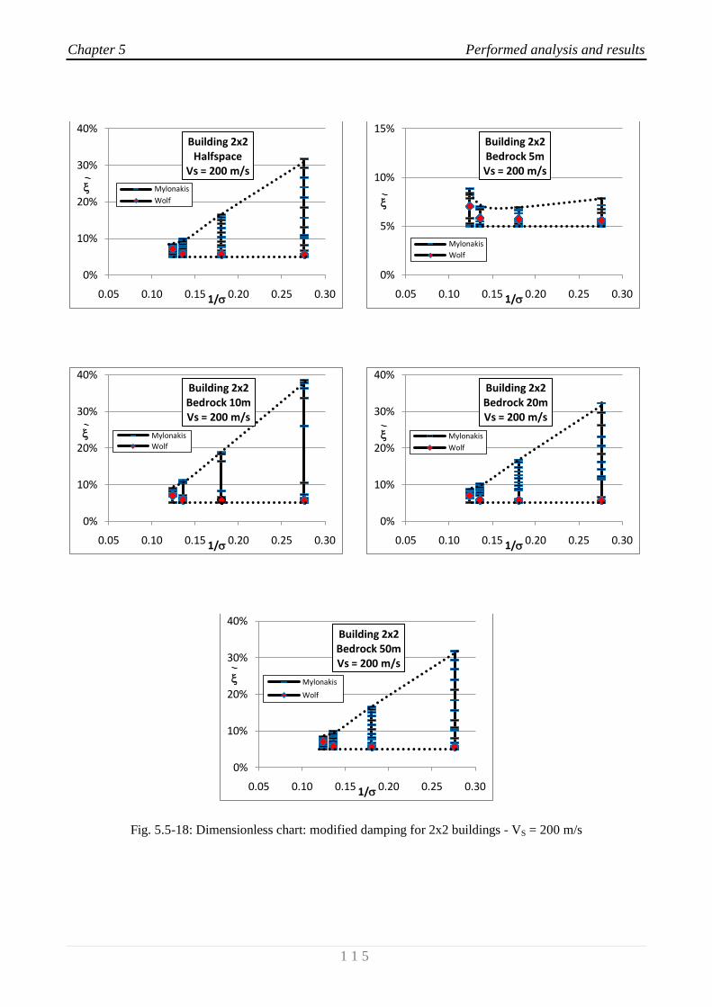
Chapter 5 Performed analysis and results
1 1 5
Fig. 5.5-18: Dimensionless chart: modified damping for 2x2 buildings - VS = 200 m/s
0%
10%
20%
30%
40%
0.05 0.10 0.15 0.20 0.25 0.30
1/
Building 2x2Halfspace
Vs = 200 m/s
Mylonakis
Wolf
0%
5%
10%
15%
0.05 0.10 0.15 0.20 0.25 0.30
1/
Building 2x2Bedrock 5mVs = 200 m/s
Mylonakis
Wolf
0%
10%
20%
30%
40%
0.05 0.10 0.15 0.20 0.25 0.30
1/
Building 2x2Bedrock 10mVs = 200 m/s
Mylonakis
Wolf
0%
10%
20%
30%
40%
0.05 0.10 0.15 0.20 0.25 0.30
1/
Building 2x2Bedrock 20mVs = 200 m/s
Mylonakis
Wolf
0%
10%
20%
30%
40%
0.05 0.10 0.15 0.20 0.25 0.30
1/
Building 2x2Bedrock 50mVs = 200 m/s
Mylonakis
Wolf
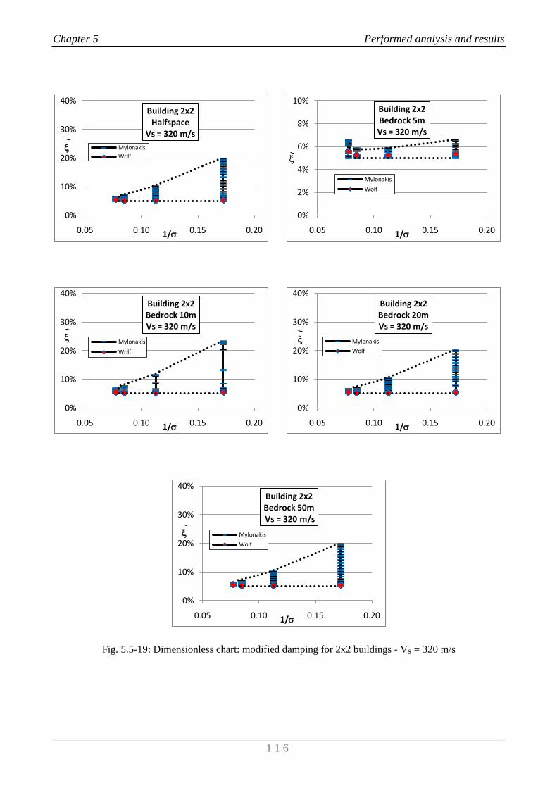
Chapter 5 Performed analysis and results
1 1 6
Fig. 5.5-19: Dimensionless chart: modified damping for 2x2 buildings - VS = 320 m/s
0%
10%
20%
30%
40%
0.05 0.10 0.15 0.20
1/
Building 2x2Halfspace
Vs = 320 m/s
Mylonakis
Wolf
0%
2%
4%
6%
8%
10%
0.05 0.10 0.15 0.20
1/
Building 2x2Bedrock 5mVs = 320 m/s
Mylonakis
Wolf
0%
10%
20%
30%
40%
0.05 0.10 0.15 0.20
1/
Building 2x2Bedrock 10mVs = 320 m/s
Mylonakis
Wolf
0%
10%
20%
30%
40%
0.05 0.10 0.15 0.20
1/
Building 2x2Bedrock 20mVs = 320 m/s
Mylonakis
Wolf
0%
10%
20%
30%
40%
0.05 0.10 0.15 0.20
1/
Building 2x2Bedrock 50mVs = 320 m/s
Mylonakis
Wolf
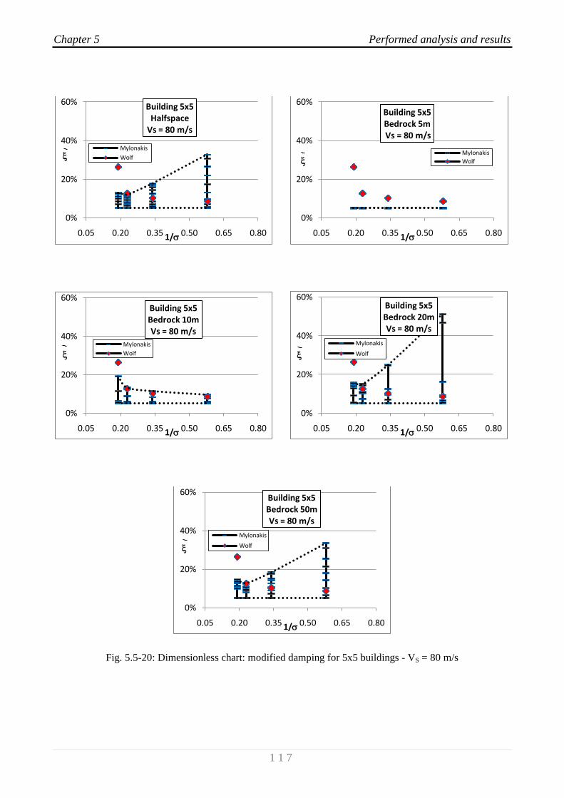
Chapter 5 Performed analysis and results
1 1 7
Fig. 5.5-20: Dimensionless chart: modified damping for 5x5 buildings - VS = 80 m/s
0%
20%
40%
60%
0.05 0.20 0.35 0.50 0.65 0.80
1/
Building 5x5Halfspace
Vs = 80 m/s
Mylonakis
Wolf
0%
20%
40%
60%
0.05 0.20 0.35 0.50 0.65 0.80
1/
Building 5x5Bedrock 5mVs = 80 m/s
Mylonakis
Wolf
0%
20%
40%
60%
0.05 0.20 0.35 0.50 0.65 0.80
1/
Building 5x5Bedrock 10mVs = 80 m/s
Mylonakis
Wolf
0%
20%
40%
60%
0.05 0.20 0.35 0.50 0.65 0.80
1/
Building 5x5Bedrock 20mVs = 80 m/s
Mylonakis
Wolf
0%
20%
40%
60%
0.05 0.20 0.35 0.50 0.65 0.80
1/
Building 5x5Bedrock 50mVs = 80 m/s
Mylonakis
Wolf
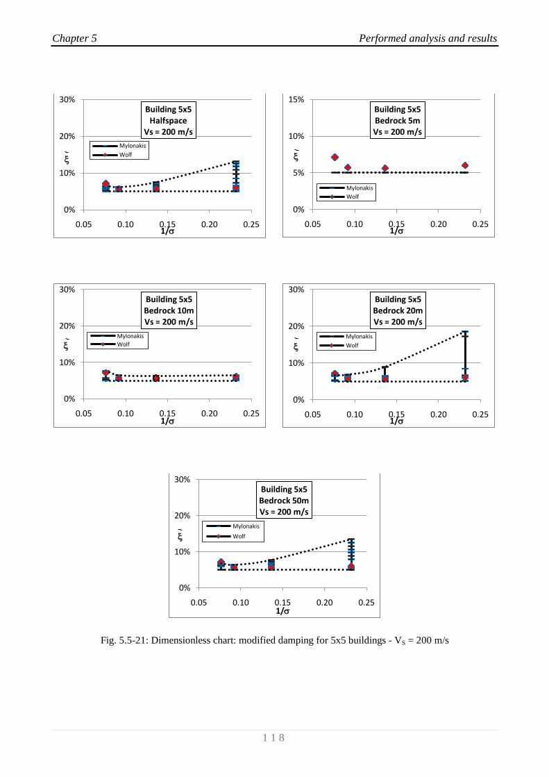
Chapter 5 Performed analysis and results
1 1 8
Fig. 5.5-21: Dimensionless chart: modified damping for 5x5 buildings - VS = 200 m/s
0%
10%
20%
30%
0.05 0.10 0.15 0.20 0.25
1/
Building 5x5Halfspace
Vs = 200 m/s
Mylonakis
Wolf
0%
5%
10%
15%
0.05 0.10 0.15 0.20 0.25
1/
Building 5x5Bedrock 5mVs = 200 m/s
Mylonakis
Wolf
0%
10%
20%
30%
0.05 0.10 0.15 0.20 0.25
1/
Building 5x5Bedrock 10mVs = 200 m/s
Mylonakis
Wolf
0%
10%
20%
30%
0.05 0.10 0.15 0.20 0.25
1/
Building 5x5Bedrock 20mVs = 200 m/s
Mylonakis
Wolf
0%
10%
20%
30%
0.05 0.10 0.15 0.20 0.25
1/
Building 5x5Bedrock 50mVs = 200 m/s
Mylonakis
Wolf

Chapter 5 Performed analysis and results
1 1 9
Fig. 5.5-22: Dimensionless chart: modified damping for 5x5 buildings - VS = 320 m/s
0%
5%
10%
15%
20%
0.00 0.05 0.10 0.15
1/
Building 5x5Halfspace
Vs = 320 m/s
Mylonakis
Wolf
0%
2%
4%
6%
8%
10%
0.00 0.05 0.10 0.15
1/
Building 5x5Bedrock 5mVs = 320 m/s
Mylonakis
Wolf
0%
5%
10%
15%
20%
0.00 0.05 0.10 0.15
1/
Building 5x5Bedrock 10mVs = 320 m/s
Mylonakis
Wolf
0%
5%
10%
15%
20%
0.00 0.05 0.10 0.15
1/
Building 5x5Bedrock 20mVs = 320 m/s
Mylonakis
Wolf
0%
5%
10%
15%
20%
0.00 0.05 0.10 0.15
1/
Building 5x5Bedrock 50mVs = 320 m/s
Mylonakis
Wolf

Chapter 5 Performed analysis and results
1 2 0
Fig. 5.5-23: Dimensionless chart: modified damping for 10x10 buildings - VS = 80 m/s
0%
20%
40%
60%
0.0 0.2 0.4 0.6
1/
Building 10x10Halfspace
Vs = 80 m/s
Mylonakis
Wolf
0%
20%
40%
60%
0.0 0.2 0.4 0.6
1/
Building 10x10Bedrock 5mVs = 80 m/s
Mylonakis
Wolf
0%
20%
40%
60%
0.0 0.2 0.4 0.6
1/
Building 10x10Bedrock 10mVs = 80 m/s
Mylonakis
Wolf
0%
20%
40%
60%
0.0 0.2 0.4 0.6
1/
Building 10x10Bedrock 20mVs = 80 m/s
Mylonakis
Wolf
0%
20%
40%
60%
0.0 0.2 0.4 0.6
1/
Building 10x10Bedrock 50mVs = 80 m/s
Mylonakis
Wolf
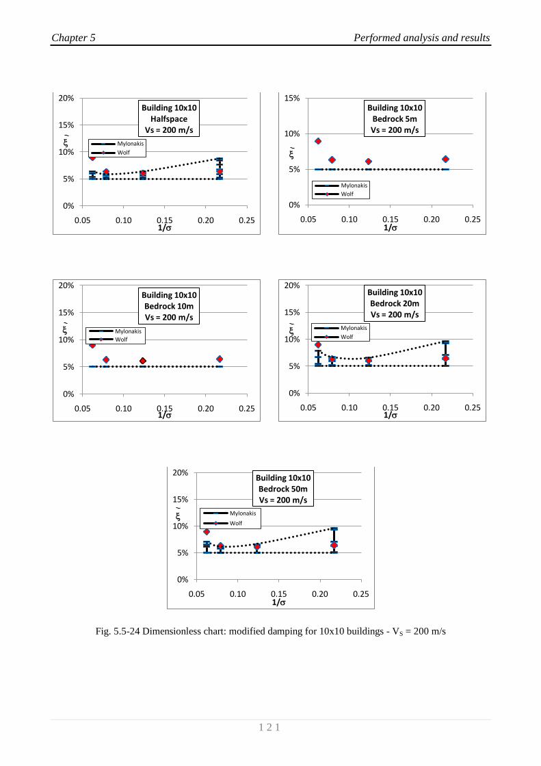
Chapter 5 Performed analysis and results
1 2 1
Fig. 5.5-24 Dimensionless chart: modified damping for 10x10 buildings - VS = 200 m/s
0%
5%
10%
15%
20%
0.05 0.10 0.15 0.20 0.25
1/
Building 10x10Halfspace
Vs = 200 m/s
Mylonakis
Wolf
0%
5%
10%
15%
0.05 0.10 0.15 0.20 0.25
1/
Building 10x10Bedrock 5mVs = 200 m/s
Mylonakis
Wolf
0%
5%
10%
15%
20%
0.05 0.10 0.15 0.20 0.25
1/
Building 10x10Bedrock 10mVs = 200 m/s
Mylonakis
Wolf
0%
5%
10%
15%
20%
0.05 0.10 0.15 0.20 0.25
1/
Building 10x10Bedrock 20mVs = 200 m/s
Mylonakis
Wolf
0%
5%
10%
15%
20%
0.05 0.10 0.15 0.20 0.25
1/
Building 10x10Bedrock 50mVs = 200 m/s
Mylonakis
Wolf
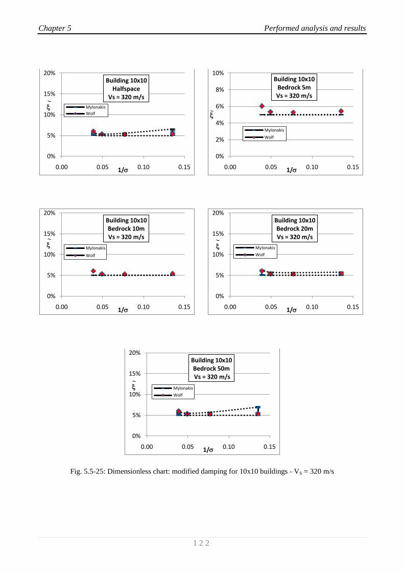
Chapter 5 Performed analysis and results
1 2 2
Fig. 5.5-25: Dimensionless chart: modified damping for 10x10 buildings - VS = 320 m/s
0%
5%
10%
15%
20%
0.00 0.05 0.10 0.15
1/
Building 10x10Halfspace
Vs = 320 m/s
Mylonakis
Wolf
0%
2%
4%
6%
8%
10%
0.00 0.05 0.10 0.15
1/
Building 10x10Bedrock 5mVs = 320 m/s
Mylonakis
Wolf
0%
5%
10%
15%
20%
0.00 0.05 0.10 0.15
1/
Building 10x10Bedrock 10mVs = 320 m/s
Mylonakis
Wolf
0%
5%
10%
15%
20%
0.00 0.05 0.10 0.15
1/
Building 10x10Bedrock 20mVs = 320 m/s
Mylonakis
Wolf
0%
5%
10%
15%
20%
0.00 0.05 0.10 0.15
1/
Building 10x10Bedrock 50mVs = 320 m/s
Mylonakis
Wolf
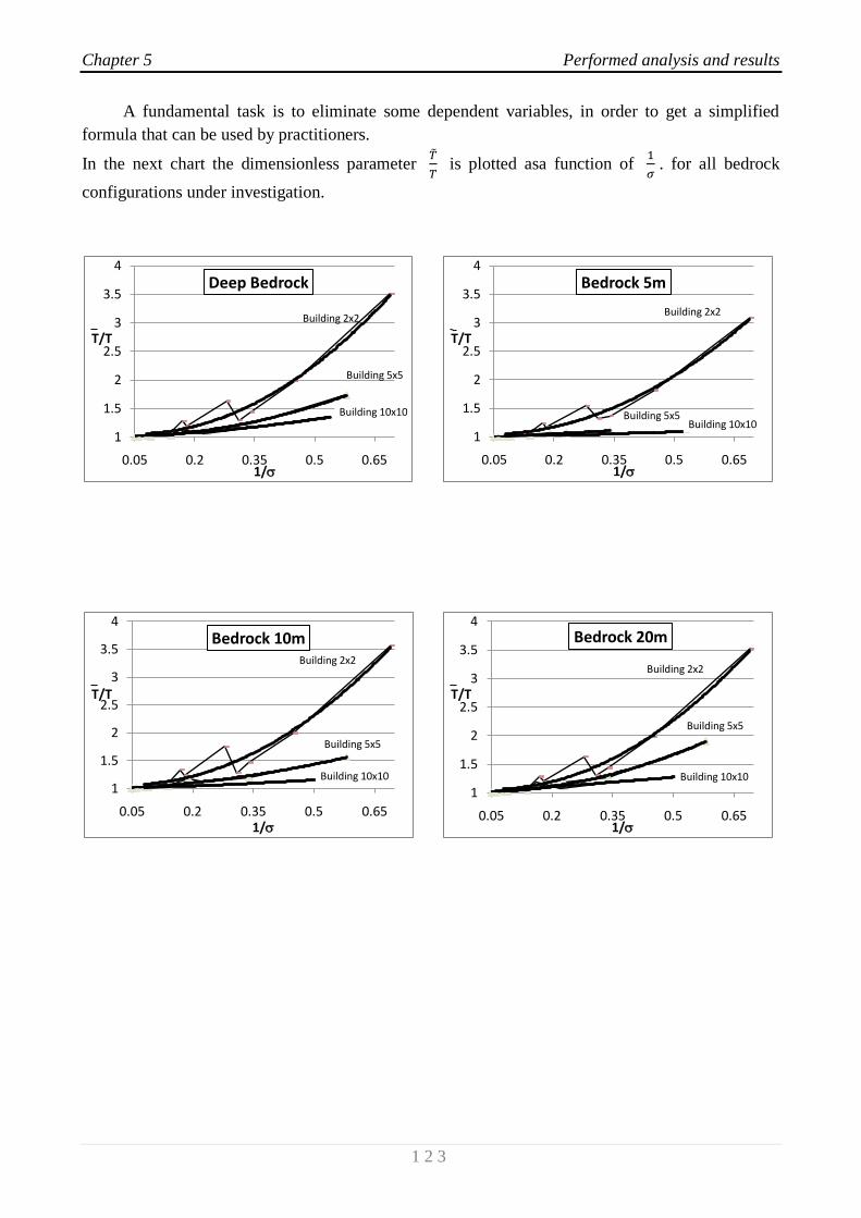
Chapter 5 Performed analysis and results
1 2 3
A fundamental task is to eliminate some dependent variables, in order to get a simplified
formula that can be used by practitioners.
In the next chart the dimensionless parameter
is plotted asa function of
. for all bedrock
configurations under investigation.
Building 2x2
Building 5x5
Building 10x10
1
1.5
2
2.5
3
3.5
4
0.05 0.2 0.35 0.5 0.65
T/T
1/
Deep Bedrock
Building 2x2
Building 5x5Building 10x10
1
1.5
2
2.5
3
3.5
4
0.05 0.2 0.35 0.5 0.65
T/T
1/
Bedrock 5m
Building 2x2
Building 5x5
Building 10x101
1.5
2
2.5
3
3.5
4
0.05 0.2 0.35 0.5 0.65
T/T
1/
Bedrock 10m
Building 2x2
Building 5x5
Building 10x10
1
1.5
2
2.5
3
3.5
4
0.05 0.2 0.35 0.5 0.65
T/T
1/
Bedrock 20m

Chapter 5 Performed analysis and results
1 2 4
5.6 Seismic SSI analyses
This research work is focused on the comparison of the results obtained from the fixed-base
(without considering SSI) and SSI configurations of concrete shear-buildings under investigations.
In particular the analyses consist of:
Eurocode 8 – part I
Without considering SSI
h/r = 0.2 8.2
1/ = 0.05 0.69
= 0.06 0.19
= 0.33 2.94
Result in term of Sa and Sd
Considering SSI
h/r = 0.2 8.2
1/ = 0.05 0.69
= 0.06 0.19
= 0.33 2.94
Result in term of
Near-Fault actual
earthquakes
Without considering SSI
h/r = 0.2 8.2
1/ = 0.12 0.69
= 0.12 0.19
= 0.33 1.89
Result in term of Sa and Sd
Considering SSI
h/r = 0.2 8.2
1/ = 0.12 0.69
= 0.12 0.19
= 0.33 1.89
Result in term of

Chapter 5 Performed analysis and results
1 2 5
5.6.1 Results from EC8-I design spectra
In this research work, in order to make a consistent comparison with the numerical results
obtained applying actual near-fault recordings (see § 5.2.2) by means of the computer program
SASSI2000, the solutions in term of seismic demand at the top of the generalized SDOF system
resulting from the application of EC8-I, are those obtained by the direct estimation of the elastic
pseudo acceleration/displacement design spectra ordinates, taking into account the changing in the
natural period and damping of the Soil-Structure systems under investigation.
To build EC8-I pseudo acceleration reference spectral shapes the following equations are
introduced in the Code:
and the previous parameter are set as
Table 5.6-1: Values of the parameters describing the recommended elastic type 1
EC8 response spectra
Table 5.6-2: VS,30 values for main site classes according to EC8-I
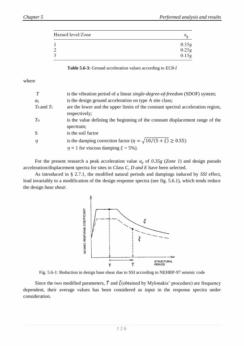
Chapter 5 Performed analysis and results
1 2 6
Table 5.6-3: Ground acceleration values according to EC8-I
where
T is the vibration period of a linear single-degree-of-freedom (SDOF) system;
ag is the design ground acceleration on type A site class;
TB and TC are the lower and the upper limits of the constant spectral acceleration region,
respectively;
TD is the value defining the beginning of the constant displacement range of the
spectrum;
S is the soil factor
is the damping correction factor (
= 1 for viscous damping = 5%).
For the present research a peak acceleration value ag of 0.35g (Zone 1) and design pseudo
acceleration/displacement spectra for sites in Class C, D and E have been selected.
As introduced in § 2.7.1, the modified natural periods and dampings induced by SSI effect,
lead invariably to a modification of the design response spectra (see fig. 5.6.1), which tends reduce
the design base shear.
Fig. 5.6-1: Reduction in design base shear due to SSI according to NEHRP-97 seismic code
Since the two modified parameters, and (obtained by Mylonakis’ procedure) are frequency
dependent, their average values has been considered as input in the response spectra under
consideration.
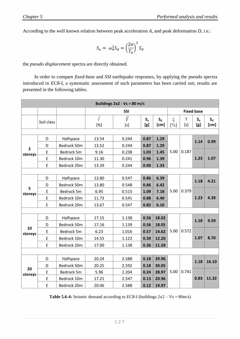
Chapter 5 Performed analysis and results
1 2 7
According to the well known relation between peak acceleration A, and peak deformation D, i.e.:
the pseudo displacement spectra are directly obtained.
In order to compare fixed-base and SSI earthquake responses, by applying the pseudo spectra
introduced in EC8-I, a systematic assessment of such parameters has been carried out; results are
presented in the following tables.
Buildings 2x2 - Vs = 80 m/s
SSI Fixed base
Soil class
[%]
[s]
Sa
[g] Sd
[cm]
T [s]
Sa
[g] Sd
[cm]
2 storeys
D Halfspace 13.54 0.244 0.87 1.29
5.00 0.187
1.14 0.99 D Bedrock 50m 13.52 0.244 0.87 1.29
E Bedrock 5m 9.16 0.238 1.03 1.45
1.23 1.07 E Bedrock 10m 11.30 0.241 0.96 1.39
E Bedrock 20m 13.39 0.244 0.90 1.33
5 storeys
D Halfspace 13.80 0.547 0.86 6.39
5.00 0.379
1.18 4.21 D Bedrock 50m 13.80 0.548 0.86 6.42
E Bedrock 5m 6.95 0.515 1.09 7.18
1.23 4.39 E Bedrock 10m 11.73 0.541 0.88 6.40
E Bedrock 20m 13.67 0.547 0.82 6.10
10 storeys
D Halfspace 17.15 1.138 0.56 18.02
5.00 0.572
1.18 9.59 D Bedrock 50m 17.16 1.139 0.56 18.05
E Bedrock 5m 6.23 1.016 0.57 14.62
1.07 8.70 E Bedrock 10m 14.55 1.122 0.39 12.20
E Bedrock 20m 17.00 1.138 0.36 11.59
20 storeys
D Halfspace 20.24 2.588 0.18 29.96
5.00 0.741
1.18 16.10 D Bedrock 50m 20.25 2.592 0.18 30.05
E Bedrock 5m 5.96 2.204 0.24 28.97
0.83 11.32 E Bedrock 10m 17.21 2.547 0.13 20.96
E Bedrock 20m 20.06 2.588 0.12 19.97
Table 5.6-4: Seismic demand according to EC8-I (buildings 2x2 – Vs = 80m/s)
~
T~

Chapter 5 Performed analysis and results
1 2 8
Buildings 5x5 - Vs = 80 m/s
SSI Fixed base
Soil class
[%]
[s]
Sa
[g] Sd
[cm]
T [s]
Sa
[g] Sd
[cm]
2 storeys
D Halfspace 10.57 0.337 0.95 2.68
5.00 0.299
1.18 2.62 D Bedrock 50m 10.72 0.338 0.94 2.67
E Bedrock 5m 5.05 0.320 1.22 3.10
1.23 2.73 E Bedrock 10m 7.30 0.328 1.10 3.16
E Bedrock 20m 10.16 0.337 0.99 2.79
5 storeys
D Halfspace 9.27 0.633 0.99 9.86
5.00 0.569
1.18 9.49 D Bedrock 50m 9.35 0.634 0.99 9.89
E Bedrock 5m 5.03 0.601 1.02 9.16
1.08 8.69 E Bedrock 10m 6.37 0.628 0.91 8.92
E Bedrock 20m 8.90 0.635 0.82 8.22
10 storeys
D Halfspace 11.43 0.945 0.78 17.31
5.00 0.766
1.18 17.20 D Bedrock 50m 11.49 0.946 0.78 17.35
E Bedrock 5m 5.04 0.847 0.72 12.84
0.80 11.66 E Bedrock 10m 6.11 0.905 0.64 13.03
E Bedrock 20m 10.84 0.954 0.51 11.53
20 storeys
D Halfspace 17.01 1.594 0.40 25.25
5.00 0.910
1.04 21.40 D Bedrock 50m 17.04 1.597 0.40 25.35
E Bedrock 5m 5.07 1.220 0.50 18.49
0.67 13.79 E Bedrock 10m 5.91 1.396 0.42 20.34
E Bedrock 20m 15.85 1.500 0.28 15.65
Table 5.6-5: Seismic demand according to EC8-I (buildings 5x5 – Vs = 80m/s)
~
T~

Chapter 5 Performed analysis and results
1 2 9
Buildings 10x10 - Vs = 80 m/s
SSI Fixed base
Soil class
[%]
[s]
Sa
[g] Sd
[cm]
T [s]
Sa
[g] Sd
[cm]
2 storeys
D Halfspace 10.80 0.413 0.94 3.98
5.00 0.365
1.18 3.91 D Bedrock 50m 10.67 0.411 0.94 3.95
E Bedrock 5m 5.01 0.381 1.22 4.40
1.23 4.07 E Bedrock 10m 5.07 0.393 1.22 4.68
E Bedrock 20m 8.81 0.402 1.04 4.18
5 storeys
D Halfspace 8.91 0.729 1.00 13.21
5.00 0.669
1.18 13.12 D Bedrock 50m 8.88 0.727 1.00 13.13
E Bedrock 5m 5.01 0.689 0.89 10.50
0.92 10.23 E Bedrock 10m 5.04 0.703 0.87 10.68
E Bedrock 20m 7.46 0.715 0.77 9.78
10 storeys
D Halfspace 9.87 0.969 0.80 18.67
5.00 0.856
1.10 20.03 D Bedrock 50m 10.03 0.967 0.80 18.59
E Bedrock 5m 5.01 0.890 0.69 13.58
0.72 13.11 E Bedrock 10m 5.05 0.914 0.67 13.91
E Bedrock 20m 7.22 0.968 0.57 13.27
20 storeys
D Halfspace 14.15 1.334 0.51 22.55
5.00 0.984
0.96 23.10 D Bedrock 50m 15.00 1.345 0.50 22.48
E Bedrock 5m 5.02 1.083 0.56 16.32
0.62 14.92 E Bedrock 10m 5.08 1.149 0.53 17.39
E Bedrock 20m 7.07 1.267 0.44 17.55
Table 5.6-6: Seismic demand according to EC8-I (buildings 10x10 – Vs = 80m/s)
~
T~

Chapter 5 Performed analysis and results
1 3 0
Buildings 2x2 - Vs = 200 m/s
SSI Fixed base
Soil class
[%]
[s]
Sa
[g] Sd
[cm]
T [s]
Sa
[g] Sd
[cm]
2 storeys
D Halfspace 6.92 0.196 0.91 0.87
5.00 0.187
0.97 0.84 D Bedrock 50m 6.96 0.196 0.91 0.87
E Bedrock 5m 5.83 0.195 1.18 1.11
1.23 1.07 E Bedrock 10m 6.88 0.196 1.12 1.08
E Bedrock 20m 6.92 0.196 1.12 1.07
5 storeys
D Halfspace 7.23 0.409 0.91 3.78
5.00 0.379
1.01 3.61 D Bedrock 50m 7.25 0.409 0.91 3.78
E Bedrock 5m 5.46 0.404 1.20 4.87
1.23 4.39 E Bedrock 10m 7.10 0.409 1.11 4.61
E Bedrock 20m 7.25 0.409 1.11 4.61
10 storeys
D Halfspace 9.47 0.687 0.73 8.56
5.00 0.572
1.01 8.21 D Bedrock 50m 9.50 0.687 0.73 8.56
E Bedrock 5m 5.45 0.663 0.90 9.83
1.07 8.70 E Bedrock 10m 9.17 0.687 0.75 8.82
E Bedrock 20m 9.54 0.687 0.74 8.68
20 storeys
D Halfspace 14.31 1.220 0.36 13.31
5.00 0.741
0.81 11.05 D Bedrock 50m 14.34 1.221 0.36 13.34
E Bedrock 5m 5.59 1.112 0.54 16.59
0.83 11.32 E Bedrock 10m 13.90 1.167 0.38 14.10
E Bedrock 20m 14.45 1.222 0.36 13.36
Table 5.6-7: Seismic demand according to EC8-I (buildings 2x2 – Vs = 200m/s)
~
T~
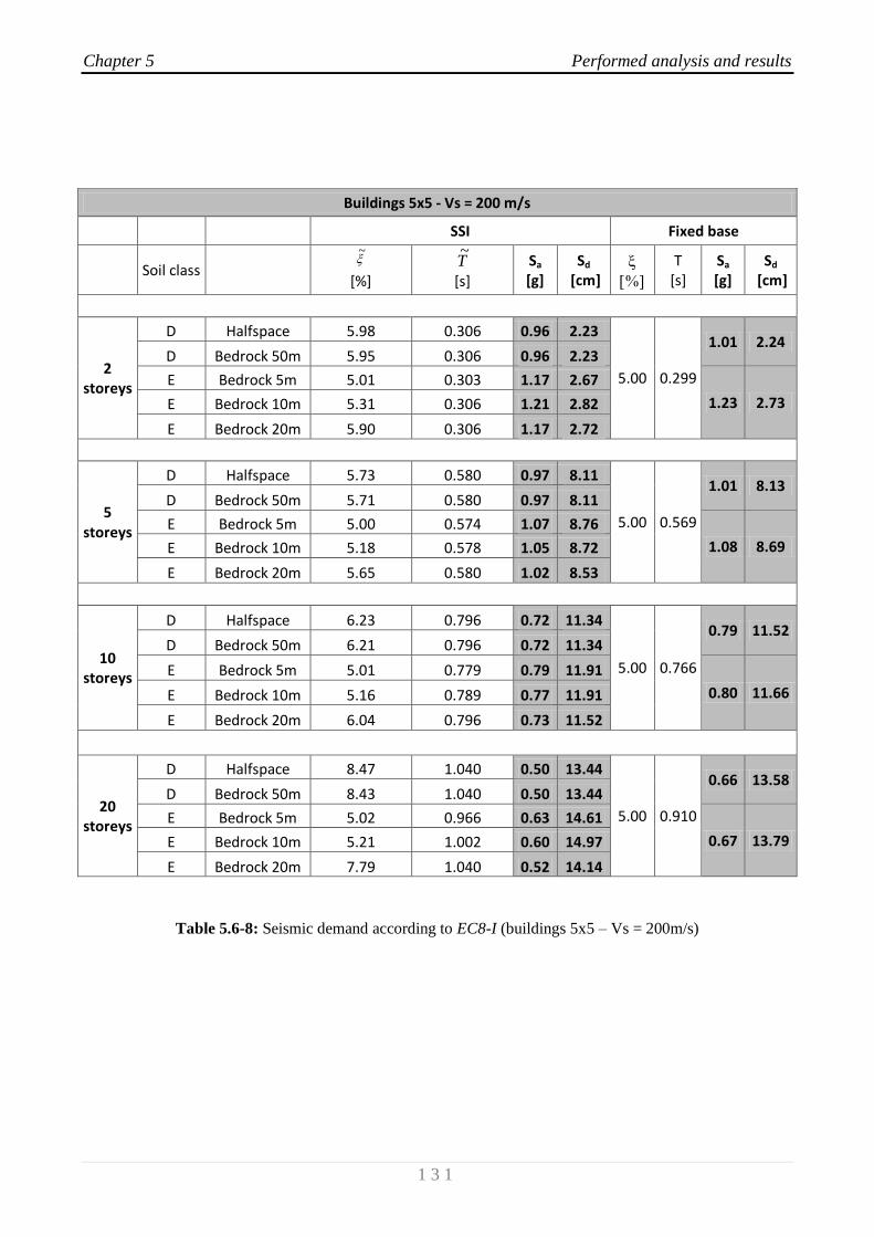
Chapter 5 Performed analysis and results
1 3 1
Buildings 5x5 - Vs = 200 m/s
SSI Fixed base
Soil class
[%]
[s]
Sa
[g] Sd
[cm]
T [s]
Sa
[g] Sd
[cm]
2 storeys
D Halfspace 5.98 0.306 0.96 2.23
5.00 0.299
1.01 2.24 D Bedrock 50m 5.95 0.306 0.96 2.23
E Bedrock 5m 5.01 0.303 1.17 2.67
1.23 2.73 E Bedrock 10m 5.31 0.306 1.21 2.82
E Bedrock 20m 5.90 0.306 1.17 2.72
5 storeys
D Halfspace 5.73 0.580 0.97 8.11
5.00 0.569
1.01 8.13 D Bedrock 50m 5.71 0.580 0.97 8.11
E Bedrock 5m 5.00 0.574 1.07 8.76
1.08 8.69 E Bedrock 10m 5.18 0.578 1.05 8.72
E Bedrock 20m 5.65 0.580 1.02 8.53
10 storeys
D Halfspace 6.23 0.796 0.72 11.34
5.00 0.766
0.79 11.52 D Bedrock 50m 6.21 0.796 0.72 11.34
E Bedrock 5m 5.01 0.779 0.79 11.91
0.80 11.66 E Bedrock 10m 5.16 0.789 0.77 11.91
E Bedrock 20m 6.04 0.796 0.73 11.52
20 storeys
D Halfspace 8.47 1.040 0.50 13.44
5.00 0.910
0.66 13.58 D Bedrock 50m 8.43 1.040 0.50 13.44
E Bedrock 5m 5.02 0.966 0.63 14.61
0.67 13.79 E Bedrock 10m 5.21 1.002 0.60 14.97
E Bedrock 20m 7.79 1.040 0.52 14.14
Table 5.6-8: Seismic demand according to EC8-I (buildings 5x5 – Vs = 200m/s)
~
T~

Chapter 5 Performed analysis and results
1 3 2
Buildings 10x10 - Vs = 200 m/s
SSI Fixed base
Soil class
[%]
[s]
Sa
[g] Sd
[cm]
T [s]
Sa
[g] Sd
[cm]
2 storeys
D Halfspace 6.04 0.373 0.96 3.32
5.00 0.365
1.01 3.34 D Bedrock 50m 5.94 0.372 0.96 3.30
E Bedrock 5m 5.00 0.367 1.23 4.12
1.23 4.07 E Bedrock 10m 5.01 0.369 1.22 4.13
E Bedrock 20m 5.63 0.373 1.19 4.16
5 storeys
D Halfspace 5.67 0.679 0.86 9.85
5.00 0.669
0.90 10.01 D Bedrock 50m 5.62 0.678 0.86 9.82
E Bedrock 5m 5.00 0.673 0.91 10.24
0.92 10.23 E Bedrock 10m 5.01 0.675 0.91 10.30
E Bedrock 20m 5.37 0.678 0.88 10.14
10 storeys
D Halfspace 5.88 0.875 0.66 12.56
5.00 0.856
0.71 12.93 D Bedrock 50m 5.84 0.874 0.66 12.53
E Bedrock 5m 5.00 0.862 0.71 13.11
0.72 13.11 E Bedrock 10m 5.01 0.866 0.71 13.23
E Bedrock 20m 5.35 0.874 0.69 13.10
20 storeys
D Halfspace 7.07 1.044 0.53 14.35
5.00 0.984
0.61 14.68 D Bedrock 50m 7.11 1.043 0.53 14.33
E Bedrock 5m 5.00 1.000 0.61 15.16
0.62 14.92 E Bedrock 10m 5.01 1.012 0.60 15.27
E Bedrock 20m 7.11 1.043 0.53 14.33
Table 5.6-9: Seismic demand according to EC8-I (buildings 10x10 – Vs = 200m/s)
~
T~
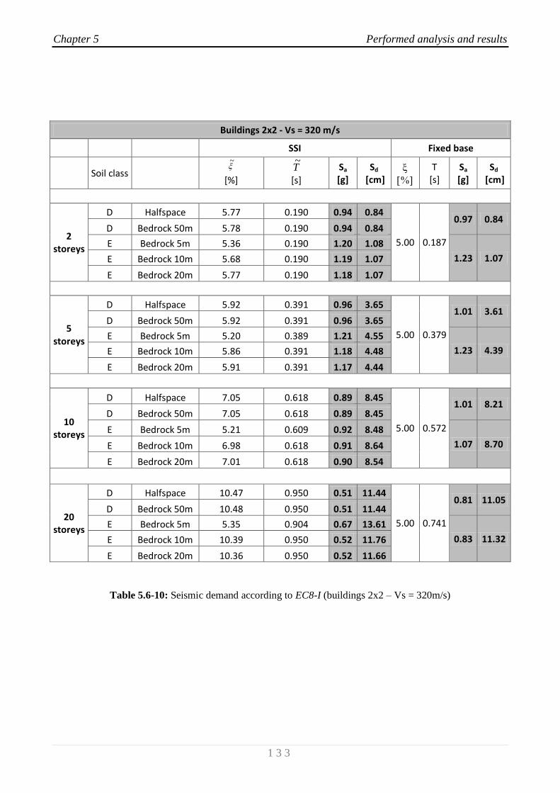
Chapter 5 Performed analysis and results
1 3 3
Buildings 2x2 - Vs = 320 m/s
SSI Fixed base
Soil class
[%]
[s]
Sa
[g] Sd
[cm]
T [s]
Sa
[g] Sd
[cm]
2 storeys
D Halfspace 5.77 0.190 0.94 0.84
5.00 0.187
0.97 0.84 D Bedrock 50m 5.78 0.190 0.94 0.84
E Bedrock 5m 5.36 0.190 1.20 1.08
1.23 1.07 E Bedrock 10m 5.68 0.190 1.19 1.07
E Bedrock 20m 5.77 0.190 1.18 1.07
5 storeys
D Halfspace 5.92 0.391 0.96 3.65
5.00 0.379
1.01 3.61 D Bedrock 50m 5.92 0.391 0.96 3.65
E Bedrock 5m 5.20 0.389 1.21 4.55
1.23 4.39 E Bedrock 10m 5.86 0.391 1.18 4.48
E Bedrock 20m 5.91 0.391 1.17 4.44
10 storeys
D Halfspace 7.05 0.618 0.89 8.45
5.00 0.572
1.01 8.21 D Bedrock 50m 7.05 0.618 0.89 8.45
E Bedrock 5m 5.21 0.609 0.92 8.48
1.07 8.70 E Bedrock 10m 6.98 0.618 0.91 8.64
E Bedrock 20m 7.01 0.618 0.90 8.54
20 storeys
D Halfspace 10.47 0.950 0.51 11.44
5.00 0.741
0.81 11.05 D Bedrock 50m 10.48 0.950 0.51 11.44
E Bedrock 5m 5.35 0.904 0.67 13.61
0.83 11.32 E Bedrock 10m 10.39 0.950 0.52 11.76
E Bedrock 20m 10.36 0.950 0.52 11.66
Table 5.6-10: Seismic demand according to EC8-I (buildings 2x2 – Vs = 320m/s)
~
T~
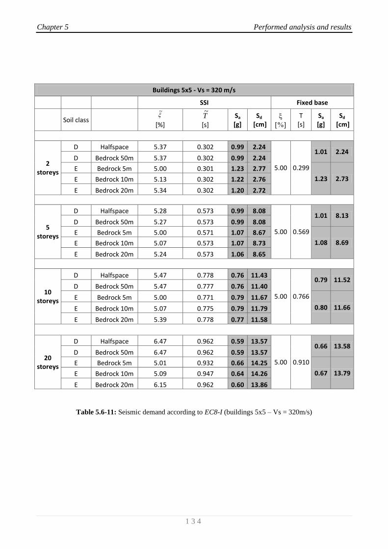
Chapter 5 Performed analysis and results
1 3 4
Buildings 5x5 - Vs = 320 m/s
SSI Fixed base
Soil class
[%]
[s]
Sa
[g] Sd
[cm]
T [s]
Sa
[g] Sd
[cm]
2 storeys
D Halfspace 5.37 0.302 0.99 2.24
5.00 0.299
1.01 2.24 D Bedrock 50m 5.37 0.302 0.99 2.24
E Bedrock 5m 5.00 0.301 1.23 2.77
1.23 2.73 E Bedrock 10m 5.13 0.302 1.22 2.76
E Bedrock 20m 5.34 0.302 1.20 2.72
5 storeys
D Halfspace 5.28 0.573 0.99 8.08
5.00 0.569
1.01 8.13 D Bedrock 50m 5.27 0.573 0.99 8.08
E Bedrock 5m 5.00 0.571 1.07 8.67
1.08 8.69 E Bedrock 10m 5.07 0.573 1.07 8.73
E Bedrock 20m 5.24 0.573 1.06 8.65
10 storeys
D Halfspace 5.47 0.778 0.76 11.43
5.00 0.766
0.79 11.52 D Bedrock 50m 5.47 0.777 0.76 11.40
E Bedrock 5m 5.00 0.771 0.79 11.67
0.80 11.66 E Bedrock 10m 5.07 0.775 0.79 11.79
E Bedrock 20m 5.39 0.778 0.77 11.58
20 storeys
D Halfspace 6.47 0.962 0.59 13.57
5.00 0.910
0.66 13.58 D Bedrock 50m 6.47 0.962 0.59 13.57
E Bedrock 5m 5.01 0.932 0.66 14.25
0.67 13.79 E Bedrock 10m 5.09 0.947 0.64 14.26
E Bedrock 20m 6.15 0.962 0.60 13.86
Table 5.6-11: Seismic demand according to EC8-I (buildings 5x5 – Vs = 320m/s)
~
T~
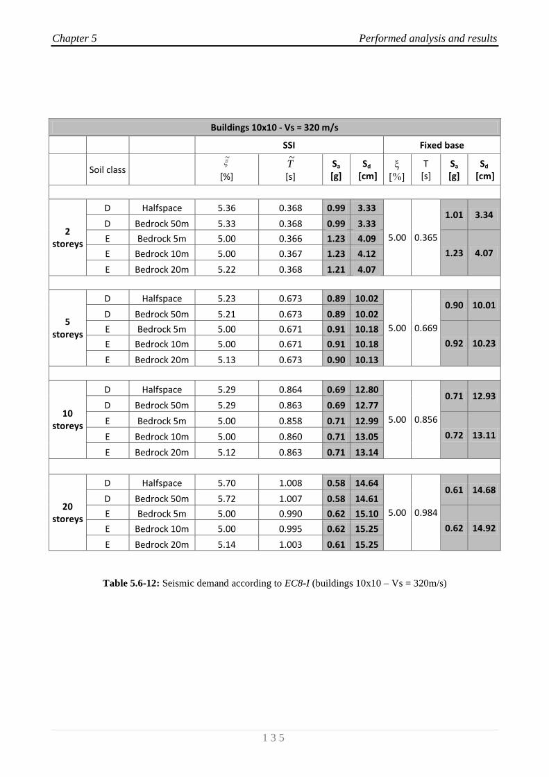
Chapter 5 Performed analysis and results
1 3 5
Buildings 10x10 - Vs = 320 m/s
SSI Fixed base
Soil class
[%]
[s]
Sa
[g] Sd
[cm]
T [s]
Sa
[g] Sd
[cm]
2 storeys
D Halfspace 5.36 0.368 0.99 3.33
5.00 0.365
1.01 3.34 D Bedrock 50m 5.33 0.368 0.99 3.33
E Bedrock 5m 5.00 0.366 1.23 4.09
1.23 4.07 E Bedrock 10m 5.00 0.367 1.23 4.12
E Bedrock 20m 5.22 0.368 1.21 4.07
5 storeys
D Halfspace 5.23 0.673 0.89 10.02
5.00 0.669
0.90 10.01 D Bedrock 50m 5.21 0.673 0.89 10.02
E Bedrock 5m 5.00 0.671 0.91 10.18
0.92 10.23 E Bedrock 10m 5.00 0.671 0.91 10.18
E Bedrock 20m 5.13 0.673 0.90 10.13
10 storeys
D Halfspace 5.29 0.864 0.69 12.80
5.00 0.856
0.71 12.93 D Bedrock 50m 5.29 0.863 0.69 12.77
E Bedrock 5m 5.00 0.858 0.71 12.99
0.72 13.11 E Bedrock 10m 5.00 0.860 0.71 13.05
E Bedrock 20m 5.12 0.863 0.71 13.14
20 storeys
D Halfspace 5.70 1.008 0.58 14.64
5.00 0.984
0.61 14.68 D Bedrock 50m 5.72 1.007 0.58 14.61
E Bedrock 5m 5.00 0.990 0.62 15.10
0.62 14.92 E Bedrock 10m 5.00 0.995 0.62 15.25
E Bedrock 20m 5.14 1.003 0.61 15.25
Table 5.6-12: Seismic demand according to EC8-I (buildings 10x10 – Vs = 320m/s)
~
T~

Chapter 5 Performed analysis and results
1 3 6
In order to get a global insight on all the results listed above, the following charts have been
prepared; the outcomes of the analyses have been grouped relating to the soil class of the deposit.
Fig. 5.6-2: Reduction in seismic demand Sa [g] due to SSI (Buildings 2x2)
Fig. 5.6-3: Reduction in seismic demand Sa [g] due to SSI (Buildings 5x5)
0.0
0.2
0.4
0.6
0.8
1.0
1.2
1.4
1.6
Sa [g]
Seismic demand - Sa [g]Buildings 2x2
Fixed base (C) SSI (C)
Fixed base (D) SSI (D)
Fixed base (E) SSI (E)
0.0
0.2
0.4
0.6
0.8
1.0
1.2
1.4
1.6
Sa [g]
Seismic demand - Sa [g]Buildings 5x5
Fixed base (C) SSI (C)
Fixed base (D) SSI (D)
Fixed base (E) SSI (E)
Soil class
C
Soil class
D
Soil class
E
Soil class
C
Soil class
D
Soil class
E
Storeys #
2 5 10 20
Storeys #
2 5 10 20
Storeys #
2 5 10 20
Storeys #
2 5 10 20
Storeys #
2 5 10 20
Storeys #
2 5 10 20
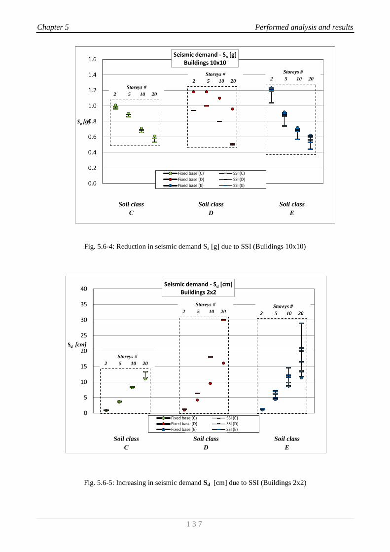
Chapter 5 Performed analysis and results
1 3 7
Fig. 5.6-4: Reduction in seismic demand Sa [g] due to SSI (Buildings 10x10)
Fig. 5.6-5: Increasing in seismic demand Sd [cm] due to SSI (Buildings 2x2)
0.0
0.2
0.4
0.6
0.8
1.0
1.2
1.4
1.6
Sa [g]
Seismic demand - Sa [g]Buildings 10x10
Fixed base (C) SSI (C)
Fixed base (D) SSI (D)
Fixed base (E) SSI (E)
0
5
10
15
20
25
30
35
40
Sd [cm]
Seismic demand - Sd [cm]Buildings 2x2
Fixed base (C) SSI (C)Fixed base (D) SSI (D)Fixed base (E) SSI (E)
Soil class
C
Soil class
D
Soil class
E
Storeys #
2 5 10 20
Storeys #
2 5 10 20
Storeys #
2 5 10 20
Soil class
C
Soil class
D
Soil class
E
Storeys #
2 5 10 20
Storeys #
2 5 10 20 Storeys #
2 5 10 20

Chapter 5 Performed analysis and results
1 3 8
Fig. 5.6-6: Increasing in seismic demand Sd [cm] due to SSI (Buildings 5x5)
Fig. 5.6-7: Increasing in seismic demand Sd [cm] due to SSI (Buildings 10x10)
0
5
10
15
20
25
30
35
40
Sd [cm]
Seismic demand - Sd [cm]Buildings 5x5
Fixed base (C) SSI (C)Fixed base (D) SSI (D)Fixed base (E) SSI (E)
0
5
10
15
20
25
30
35
40
Sd [cm]
Seismic demand - Sd [cm]Buildings 10x10
Fixed base (C) SSI (C)Fixed base (D) SSI (D)Fixed base (E) SSI (E)
Soil class
C
Soil class
D
Soil class
E
Storeys #
2 5 10 20
Storeys #
2 5 10 20
Storeys #
2 5 10 20
Soil class
C
Soil class
D
Soil class
E
Storeys #
2 5 10 20
Storeys #
2 5 10 20
Storeys #
2 5 10 20
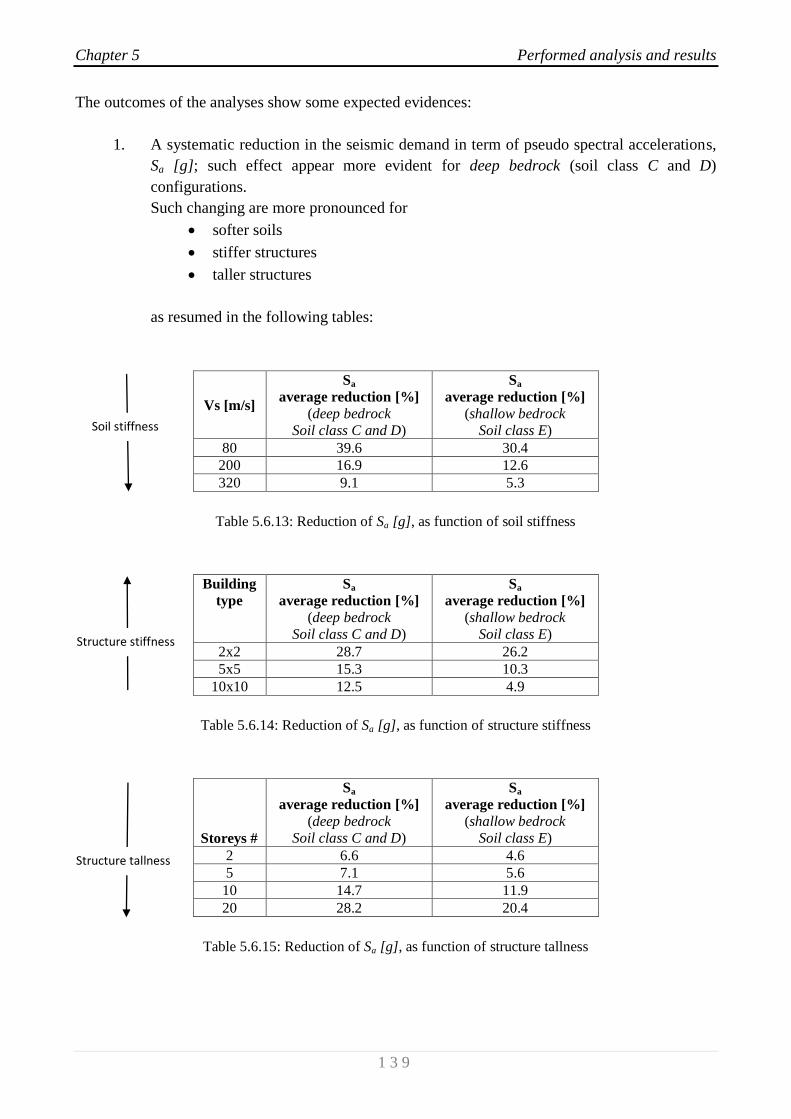
Chapter 5 Performed analysis and results
1 3 9
The outcomes of the analyses show some expected evidences:
1. A systematic reduction in the seismic demand in term of pseudo spectral accelerations,
Sa [g]; such effect appear more evident for deep bedrock (soil class C and D)
configurations.
Such changing are more pronounced for
softer soils
stiffer structures
taller structures
as resumed in the following tables:
Vs [m/s]
Sa
average reduction [%]
(deep bedrock
Soil class C and D)
Sa
average reduction [%]
(shallow bedrock
Soil class E)
80 39.6 30.4
200 16.9 12.6
320 9.1 5.3
Table 5.6.13: Reduction of Sa [g], as function of soil stiffness
Building
type
Sa
average reduction [%]
(deep bedrock
Soil class C and D)
Sa
average reduction [%]
(shallow bedrock
Soil class E)
2x2 28.7 26.2
5x5 15.3 10.3
10x10 12.5 4.9
Table 5.6.14: Reduction of Sa [g], as function of structure stiffness
Storeys #
Sa
average reduction [%]
(deep bedrock
Soil class C and D)
Sa
average reduction [%]
(shallow bedrock
Soil class E)
2 6.6 4.6
5 7.1 5.6
10 14.7 11.9
20 28.2 20.4
Table 5.6.15: Reduction of Sa [g], as function of structure tallness
Soil stiffness
Structure stiffness
Structure tallness
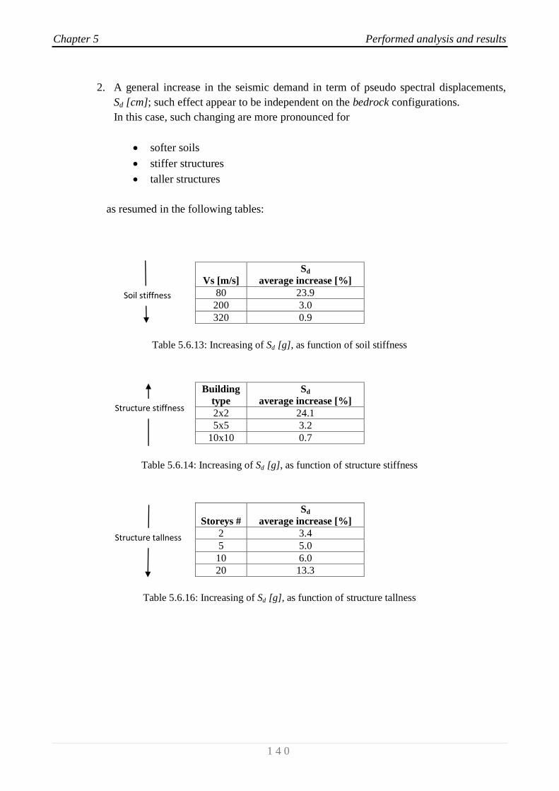
Chapter 5 Performed analysis and results
1 4 0
2. A general increase in the seismic demand in term of pseudo spectral displacements,
Sd [cm]; such effect appear to be independent on the bedrock configurations.
In this case, such changing are more pronounced for
softer soils
stiffer structures
taller structures
as resumed in the following tables:
Vs [m/s]
Sd
average increase [%]
80 23.9
200 3.0
320 0.9
Table 5.6.13: Increasing of Sd [g], as function of soil stiffness
Building
type
Sd
average increase [%]
2x2 24.1
5x5 3.2
10x10 0.7
Table 5.6.14: Increasing of Sd [g], as function of structure stiffness
Storeys #
Sd
average increase [%]
2 3.4
5 5.0
10 6.0
20 13.3
Table 5.6.16: Increasing of Sd [g], as function of structure tallness
Soil stiffness
Structure stiffness
Structure tallness
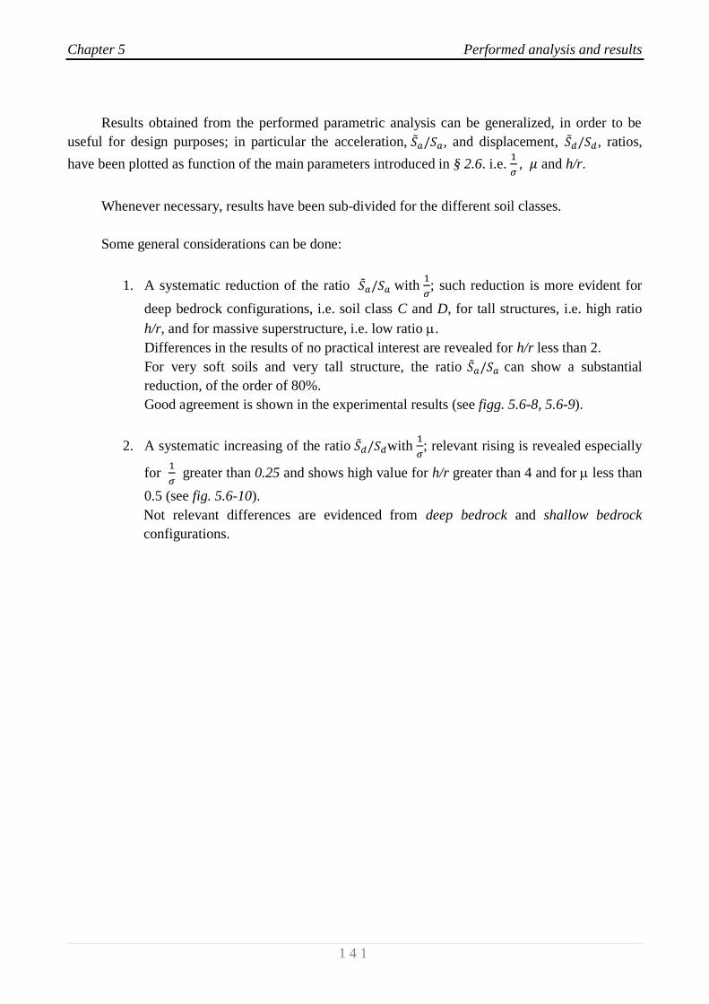
Chapter 5 Performed analysis and results
1 4 1
Results obtained from the performed parametric analysis can be generalized, in order to be
useful for design purposes; in particular the acceleration, , and displacement, , ratios,
have been plotted as function of the main parameters introduced in § 2.6. i.e.
and h/r.
Whenever necessary, results have been sub-divided for the different soil classes.
Some general considerations can be done:
1. A systematic reduction of the ratio with
; such reduction is more evident for
deep bedrock configurations, i.e. soil class C and D, for tall structures, i.e. high ratio
h/r, and for massive superstructure, i.e. low ratio .
Differences in the results of no practical interest are revealed for h/r less than 2.
For very soft soils and very tall structure, the ratio can show a substantial
reduction, of the order of 80%.
Good agreement is shown in the experimental results (see figg. 5.6-8, 5.6-9).
2. A systematic increasing of the ratio with
; relevant rising is revealed especially
for
greater than 0.25 and shows high value for h/r greater than 4 and for less than
0.5 (see fig. 5.6-10).
Not relevant differences are evidenced from deep bedrock and shallow bedrock
configurations.

Chapter 5 Performed analysis and results
1 4 2
Fig. 5.6-8: as function of 1/ and h/rsoil class C - D
Fig. 5.6-9: as function of 1/ and h/rsoil class E
h/r = 0.22
(or = 0.673)
h/r =3.54
(or = 0.5)
h/r = 8
or ( = 0.33)
0.0
0.2
0.4
0.6
0.8
1.0
1.2
0.0 0.1 0.2 0.3 0.4 0.5 0.6 0.7
Sa/Sa
1/
Soil Class C - D
str = 5%, g = 0.3, g = 5%, = 0.060.20, = 0.333
h/r = 0.22
or ( = 0.673)
h/r =3.54
(or = 0.5)
h/r = 8
or ( = 0.33)
0.0
0.2
0.4
0.6
0.8
1.0
1.2
0.0 0.1 0.2 0.3 0.4 0.5 0.6 0.7
Sa/Sa
1/
Soil Class E
str = 5%, g = 0.3, g = 5%, = 0.060.20, = 0.333
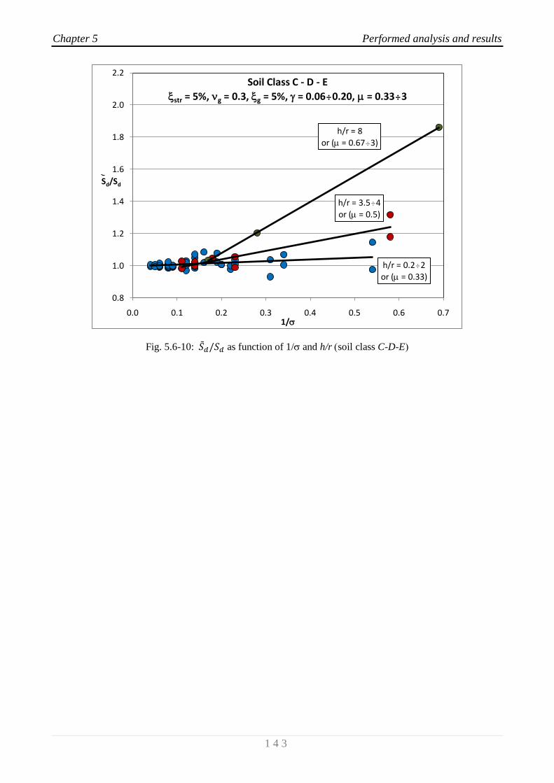
Chapter 5 Performed analysis and results
1 4 3
Fig. 5.6-10: as function of 1/and h/rsoil class C-D-E
h/r = 0.22
or ( = 0.33)
h/r = 3.54
or ( = 0.5)
h/r = 8
or ( = 0.673)
0.8
1.0
1.2
1.4
1.6
1.8
2.0
2.2
0.0 0.1 0.2 0.3 0.4 0.5 0.6 0.7
Sd/Sd
1/
Soil Class C - D - E
str = 5%, g = 0.3, g = 5%, = 0.060.20, = 0.333

Chapter 5 Performed analysis and results
1 4 4
5.6.2 Results from actual Near-Fault earthquakes
The near-fault strong ground motion database that we have compiled consists of 10 processed
near-field strong ground motion records from a variety of tectonic environments.
The database of actual recorded ground-motion time histories, from different fault types (i.e.,
strike-slip, reverse, oblique) and earthquake magnitudes (i.e., Mw 5.6–6.7), has been compiled from
well known and extensively studied seismic events that have occurred mostly in the United States,
but also in Canada and Turkey:
Parkfield, CA, USA (Station CO2)
San Fernando, CA, USA (Station PCD)
Coyote Lake, CA, USA (Station GA6)
Imperial Valley, CA, USA (Station E07)
Morgan Hill, CA, USA (Station CLD)
Nahanni, Canada (Station SITE1)
Palm Spring, CA, USA (Station NPS)
Whittier Narrows, CA, USA (Station DOW)
Superstition Hills, CA, USA (Station, ELC)
Erzincan, Turkey (Station ERZ)
All the motions were recorded at stations located within 20 km from the causative fault and
distinct strong velocity pulses are recognized, with the only exception of Nahanni earthquake.
A comprehensive spreadsheet of the database is provided in Appendix B.
In figure 5.6-1 is shown the characteristic near-fault strong ground motion of two earthquake
used in the analyses, i.e. Parkfield (CO2) and San Fernando (PCD).
The analyses performed in the present research work consist in the application of all the
earthquakes listed above to the shear-buildings defined in § 5.4, founded on soil defined in § 5.3;
the analyses has been restricted to 2x2 buildings and to soil deposits with low shear-wave velocity,
i.e. VS = 80-200 m/s (Soil Class C – D). Such Soil-Structure configurations have been selected
because, as showed in § 5.6.1, stiffer structures resting on soft soils are most susceptible to the
effects imposed by Soil Structure Interaction analysis.
Results presented in tables hereinafter have not to be considered as universal outcomes of
near-fault earthquakes application; a generalization is well above the scope of the present thesis
and, for the knowledge of the author, such an attempt of generalization is inappropriate in the field
of near-fault effects; many parameters have to be carefully analyzed by seismologists, geologists
and engineers, e.g. characteristics of the causative fault, geology of the deposit, path of the
travelling waves, building typology.
Nevertheless, the analyses performed have showed some interesting results that, if carefully
interpreted, could lead some general understandings of the phenomenon.
Chapter 5 Performed analysis and results
1 4 5
Fig. 5.6-1: Characteristic near-fault strong ground motions: (a) Station 2 (C02) record obtained from the
1966 Parkfield, California, earthquake; (b) Pacoima Dam (PCD) record obtained from the 1971 San
Fernando, California, earthquake. (after Mavroeidis and Papageorgiou, 2003)
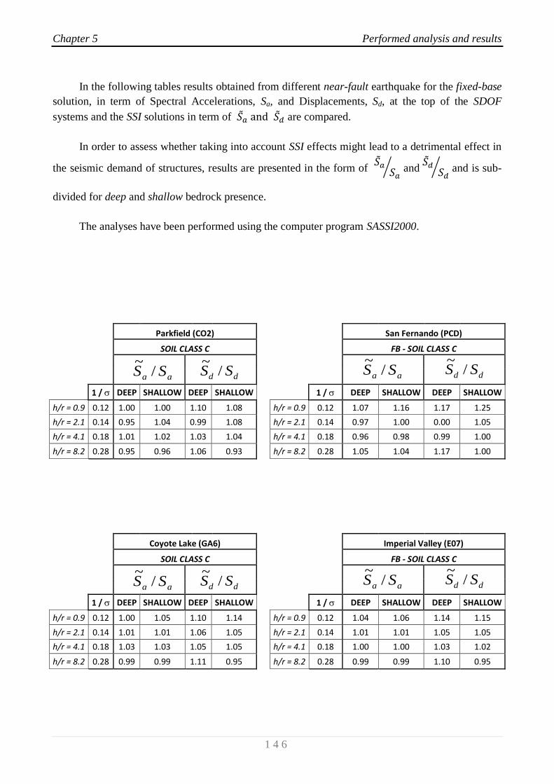
Chapter 5 Performed analysis and results
1 4 6
In the following tables results obtained from different near-fault earthquake for the fixed-base
solution, in term of Spectral Accelerations, Sa, and Displacements, Sd, at the top of the SDOF
systems and the SSI solutions in term of are compared.
In order to assess whether taking into account SSI effects might lead to a detrimental effect in
the seismic demand of structures, results are presented in the form of
and
and is sub-
divided for deep and shallow bedrock presence.
The analyses have been performed using the computer program SASSI2000.
Parkfield (CO2)
San Fernando (PCD)
SOIL CLASS C
FB - SOIL CLASS C
1 / DEEP SHALLOW DEEP SHALLOW
1 / DEEP SHALLOW DEEP SHALLOW
h/r = 0.9 0.12 1.00 1.00 1.10 1.08
h/r = 0.9 0.12 1.07 1.16 1.17 1.25
h/r = 2.1 0.14 0.95 1.04 0.99 1.08
h/r = 2.1 0.14 0.97 1.00 0.00 1.05
h/r = 4.1 0.18 1.01 1.02 1.03 1.04
h/r = 4.1 0.18 0.96 0.98 0.99 1.00
h/r = 8.2 0.28 0.95 0.96 1.06 0.93
h/r = 8.2 0.28 1.05 1.04 1.17 1.00
Coyote Lake (GA6)
Imperial Valley (E07)
SOIL CLASS C
FB - SOIL CLASS C
1 / DEEP SHALLOW DEEP SHALLOW
1 / DEEP SHALLOW DEEP SHALLOW
h/r = 0.9 0.12 1.00 1.05 1.10 1.14
h/r = 0.9 0.12 1.04 1.06 1.14 1.15
h/r = 2.1 0.14 1.01 1.01 1.06 1.05
h/r = 2.1 0.14 1.01 1.01 1.05 1.05
h/r = 4.1 0.18 1.03 1.03 1.05 1.05
h/r = 4.1 0.18 1.00 1.00 1.03 1.02
h/r = 8.2 0.28 0.99 0.99 1.11 0.95
h/r = 8.2 0.28 0.99 0.99 1.10 0.95
aa SS /~
dd SS /~
aa SS /~
dd SS /~
aa SS /~
dd SS /~
aa SS /~
dd SS /~
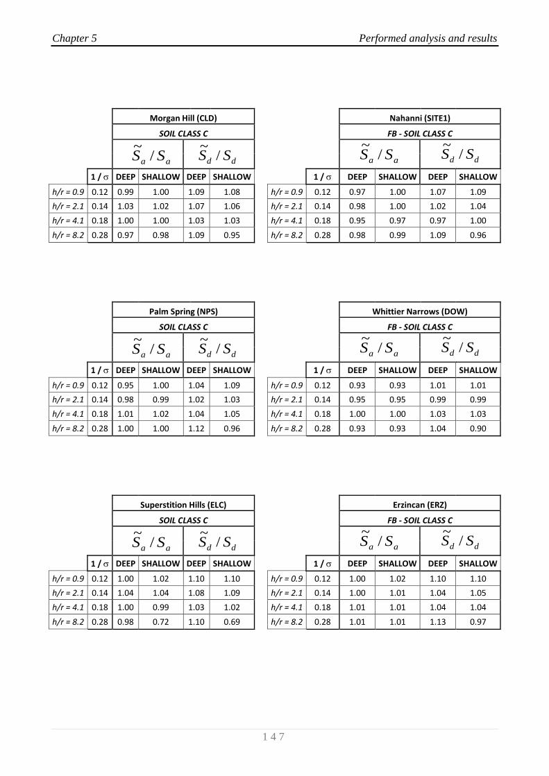
Chapter 5 Performed analysis and results
1 4 7
Morgan Hill (CLD)
Nahanni (SITE1)
SOIL CLASS C
FB - SOIL CLASS C
1 / DEEP SHALLOW DEEP SHALLOW
1 / DEEP SHALLOW DEEP SHALLOW
h/r = 0.9 0.12 0.99 1.00 1.09 1.08
h/r = 0.9 0.12 0.97 1.00 1.07 1.09
h/r = 2.1 0.14 1.03 1.02 1.07 1.06
h/r = 2.1 0.14 0.98 1.00 1.02 1.04
h/r = 4.1 0.18 1.00 1.00 1.03 1.03
h/r = 4.1 0.18 0.95 0.97 0.97 1.00
h/r = 8.2 0.28 0.97 0.98 1.09 0.95
h/r = 8.2 0.28 0.98 0.99 1.09 0.96
Palm Spring (NPS)
Whittier Narrows (DOW)
SOIL CLASS C
FB - SOIL CLASS C
1 / DEEP SHALLOW DEEP SHALLOW
1 / DEEP SHALLOW DEEP SHALLOW
h/r = 0.9 0.12 0.95 1.00 1.04 1.09
h/r = 0.9 0.12 0.93 0.93 1.01 1.01
h/r = 2.1 0.14 0.98 0.99 1.02 1.03
h/r = 2.1 0.14 0.95 0.95 0.99 0.99
h/r = 4.1 0.18 1.01 1.02 1.04 1.05
h/r = 4.1 0.18 1.00 1.00 1.03 1.03
h/r = 8.2 0.28 1.00 1.00 1.12 0.96
h/r = 8.2 0.28 0.93 0.93 1.04 0.90
Superstition Hills (ELC)
Erzincan (ERZ)
SOIL CLASS C
FB - SOIL CLASS C
1 / DEEP SHALLOW DEEP SHALLOW
1 / DEEP SHALLOW DEEP SHALLOW
h/r = 0.9 0.12 1.00 1.02 1.10 1.10
h/r = 0.9 0.12 1.00 1.02 1.10 1.10
h/r = 2.1 0.14 1.04 1.04 1.08 1.09
h/r = 2.1 0.14 1.00 1.01 1.04 1.05
h/r = 4.1 0.18 1.00 0.99 1.03 1.02
h/r = 4.1 0.18 1.01 1.01 1.04 1.04
h/r = 8.2 0.28 0.98 0.72 1.10 0.69
h/r = 8.2 0.28 1.01 1.01 1.13 0.97
aa SS /~
dd SS /~
aa SS /~
dd SS /~
aa SS /~
dd SS /~
aa SS /~
dd SS /~
aa SS /~
dd SS /~
aa SS /~
dd SS /~
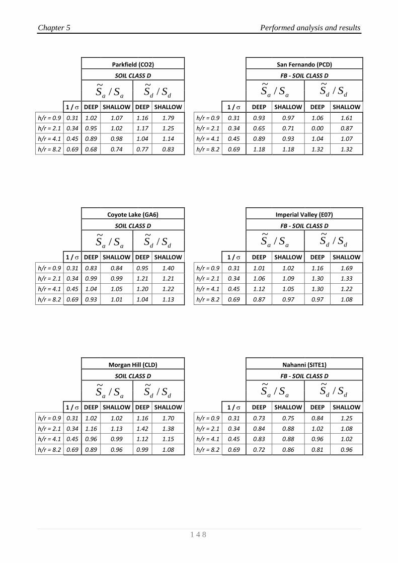
Chapter 5 Performed analysis and results
1 4 8
Parkfield (CO2)
San Fernando (PCD)
SOIL CLASS D
FB - SOIL CLASS D
1 / DEEP SHALLOW DEEP SHALLOW
1 / DEEP SHALLOW DEEP SHALLOW
h/r = 0.9 0.31 1.02 1.07 1.16 1.79
h/r = 0.9 0.31 0.93 0.97 1.06 1.61
h/r = 2.1 0.34 0.95 1.02 1.17 1.25
h/r = 2.1 0.34 0.65 0.71 0.00 0.87
h/r = 4.1 0.45 0.89 0.98 1.04 1.14
h/r = 4.1 0.45 0.89 0.93 1.04 1.07
h/r = 8.2 0.69 0.68 0.74 0.77 0.83
h/r = 8.2 0.69 1.18 1.18 1.32 1.32
Coyote Lake (GA6)
Imperial Valley (E07)
SOIL CLASS D
FB - SOIL CLASS D
1 / DEEP SHALLOW DEEP SHALLOW
1 / DEEP SHALLOW DEEP SHALLOW
h/r = 0.9 0.31 0.83 0.84 0.95 1.40
h/r = 0.9 0.31 1.01 1.02 1.16 1.69
h/r = 2.1 0.34 0.99 0.99 1.21 1.21
h/r = 2.1 0.34 1.06 1.09 1.30 1.33
h/r = 4.1 0.45 1.04 1.05 1.20 1.22
h/r = 4.1 0.45 1.12 1.05 1.30 1.22
h/r = 8.2 0.69 0.93 1.01 1.04 1.13
h/r = 8.2 0.69 0.87 0.97 0.97 1.08
Morgan Hill (CLD)
Nahanni (SITE1)
SOIL CLASS D
FB - SOIL CLASS D
1 / DEEP SHALLOW DEEP SHALLOW
1 / DEEP SHALLOW DEEP SHALLOW
h/r = 0.9 0.31 1.02 1.02 1.16 1.70
h/r = 0.9 0.31 0.73 0.75 0.84 1.25
h/r = 2.1 0.34 1.16 1.13 1.42 1.38
h/r = 2.1 0.34 0.84 0.88 1.02 1.08
h/r = 4.1 0.45 0.96 0.99 1.12 1.15
h/r = 4.1 0.45 0.83 0.88 0.96 1.02
h/r = 8.2 0.69 0.89 0.96 0.99 1.08
h/r = 8.2 0.69 0.72 0.86 0.81 0.96
aa SS /~
dd SS /~
aa SS /~
dd SS /~
aa SS /~
dd SS /~
aa SS /~
dd SS /~
aa SS /~
dd SS /~
aa SS /~
dd SS /~
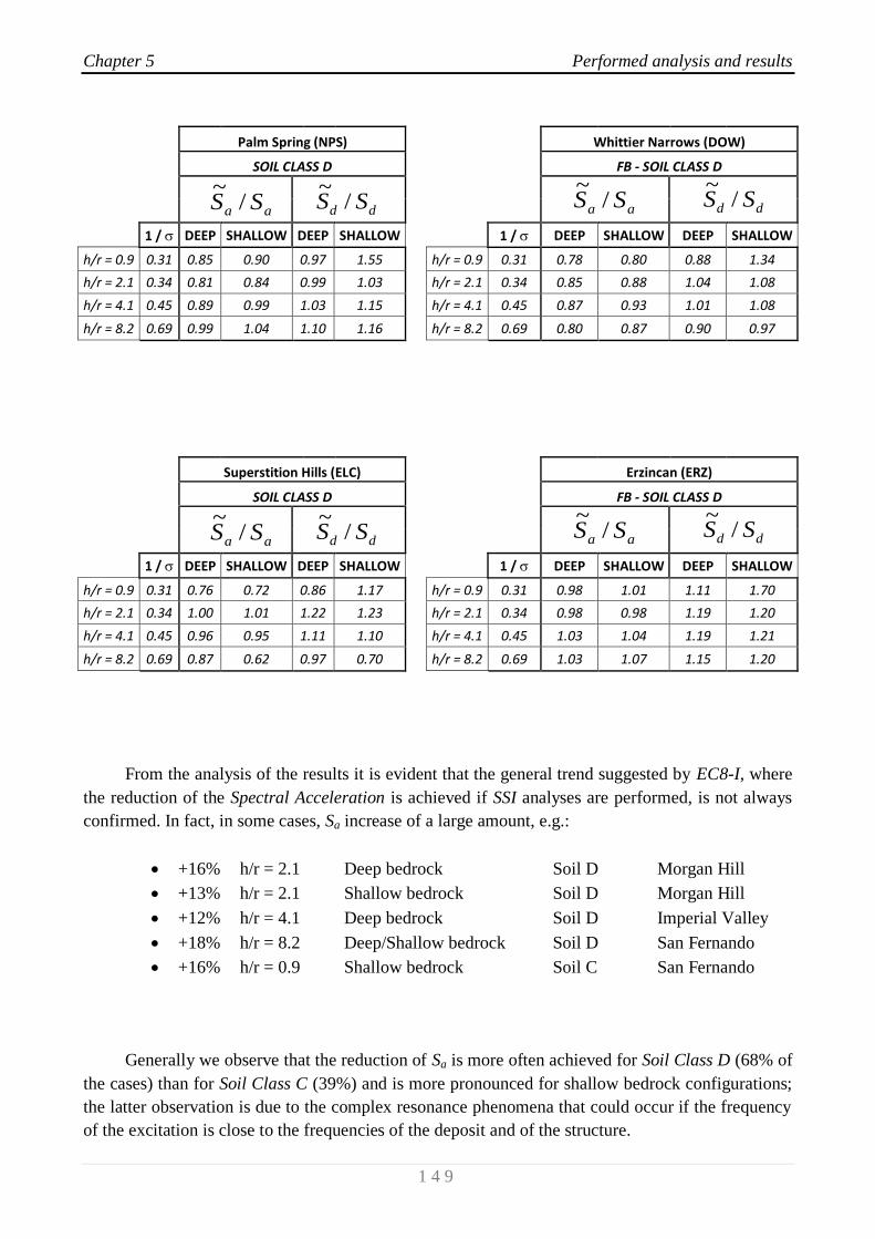
Chapter 5 Performed analysis and results
1 4 9
Palm Spring (NPS)
Whittier Narrows (DOW)
SOIL CLASS D
FB - SOIL CLASS D
1 / DEEP SHALLOW DEEP SHALLOW
1 / DEEP SHALLOW DEEP SHALLOW
h/r = 0.9 0.31 0.85 0.90 0.97 1.55
h/r = 0.9 0.31 0.78 0.80 0.88 1.34
h/r = 2.1 0.34 0.81 0.84 0.99 1.03
h/r = 2.1 0.34 0.85 0.88 1.04 1.08
h/r = 4.1 0.45 0.89 0.99 1.03 1.15
h/r = 4.1 0.45 0.87 0.93 1.01 1.08
h/r = 8.2 0.69 0.99 1.04 1.10 1.16
h/r = 8.2 0.69 0.80 0.87 0.90 0.97
Superstition Hills (ELC)
Erzincan (ERZ)
SOIL CLASS D
FB - SOIL CLASS D
1 / DEEP SHALLOW DEEP SHALLOW
1 / DEEP SHALLOW DEEP SHALLOW
h/r = 0.9 0.31 0.76 0.72 0.86 1.17
h/r = 0.9 0.31 0.98 1.01 1.11 1.70
h/r = 2.1 0.34 1.00 1.01 1.22 1.23
h/r = 2.1 0.34 0.98 0.98 1.19 1.20
h/r = 4.1 0.45 0.96 0.95 1.11 1.10
h/r = 4.1 0.45 1.03 1.04 1.19 1.21
h/r = 8.2 0.69 0.87 0.62 0.97 0.70
h/r = 8.2 0.69 1.03 1.07 1.15 1.20
From the analysis of the results it is evident that the general trend suggested by EC8-I, where
the reduction of the Spectral Acceleration is achieved if SSI analyses are performed, is not always
confirmed. In fact, in some cases, Sa increase of a large amount, e.g.:
+16% h/r = 2.1 Deep bedrock Soil D Morgan Hill
+13% h/r = 2.1 Shallow bedrock Soil D Morgan Hill
+12% h/r = 4.1 Deep bedrock Soil D Imperial Valley
+18% h/r = 8.2 Deep/Shallow bedrock Soil D San Fernando
+16% h/r = 0.9 Shallow bedrock Soil C San Fernando
Generally we observe that the reduction of Sa is more often achieved for Soil Class D (68% of
the cases) than for Soil Class C (39%) and is more pronounced for shallow bedrock configurations;
the latter observation is due to the complex resonance phenomena that could occur if the frequency
of the excitation is close to the frequencies of the deposit and of the structure.
aa SS /~
dd SS /~
aa SS /~
dd SS /~
aa SS /~
dd SS /~
aa SS /~
dd SS /~
Chapter 5 Performed analysis and results
1 5 0
Concerning the Spectral Displacement, Sd, huge increases are showed, especially for Soil
Class D and squat structures, e.g.:
+79% h/r = 0.9 Shallow bedrock Soil D Parkfield
+61% h/r = 0.9 Shallow bedrock Soil D San Fernando
+40% h/r = 0.9 Shallow bedrock Soil D Coyote Lake
+69% h/r = 0.9 Shallow bedrock Soil D Imperial Valley
+70% h/r = 0.9 Shallow bedrock Soil D Morgan Hills
+70% h/r = 0.9 Shallow bedrock Soil D Erzincan
Results listed above show that Soil Structure Interaction effect during near-fault ground
motions is a complex phenomenon that require deep local seismological, geological and
engineering investigations.
Therefore it is evident that SSI effect during near-fault events may lead to an increase of the
seismic demand, both in term of Spectral Acceleration, Sa, and of Spectral Displacement, Sd.
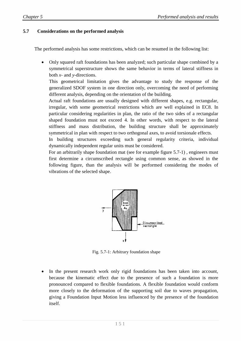
Chapter 5 Performed analysis and results
1 5 1
5.7 Considerations on the performed analysis
The performed analysis has some restrictions, which can be resumed in the following list:
Only squared raft foundations has been analyzed; such particular shape combined by a
symmetrical superstructure shows the same behavior in terms of lateral stiffness in
both x- and y-directions.
This geometrical limitation gives the advantage to study the response of the
generalized SDOF system in one direction only, overcoming the need of performing
different analysis, depending on the orientation of the building.
Actual raft foundations are usually designed with different shapes, e.g. rectangular,
irregular, with some geometrical restrictions which are well explained in EC8. In
particular considering regularities in plan, the ratio of the two sides of a rectangular
shaped foundation must not exceed 4. In other words, with respect to the lateral
stiffness and mass distribution, the building structure shall be approximately
symmetrical in plan with respect to two orthogonal axes, to avoid torsionale effects.
In building structures exceeding such general regularity criteria, individual
dynamically independent regular units must be considered.
For an arbitrarily shape foundation mat (see for example figure 5.7-1) , engineers must
first determine a circumscribed rectangle using common sense, as showed in the
following figure, than the analysis will be performed considering the modes of
vibrations of the selected shape.
Fig. 5.7-1: Arbitrary foundation shape
In the present research work only rigid foundations has been taken into account,
because the kinematic effect due to the presence of such a foundation is more
pronounced compared to flexible foundations. A flexible foundation would conform
more closely to the deformation of the supporting soil due to waves propagation,
giving a Foundation Input Motion less influenced by the presence of the foundation
itself.
Chapter 5 Performed analysis and results
1 5 2
As suggested by EC8, 5% structural damping ratio has been selected as input for the
present analysis. Considering the soil, the same damping ratio of 5% has been used at
frequency equal to zero ( = 0, static conditions); such value corresponds to a low-
medium level of soil deformation induced by the majority of seismic events expected
in Italy.
As showed in the results of the analysis, such value can highly increase due to SSI
effect, depending on the frequencies of analysis. Such increase is due to radiation and
material damping of the medium.
In order to include the different characteristics of the soil (e.g. sand/gravel and
clay/silt) it is suggested to evaluate the most suitable value of static damping ratio, that
could be generally considered higher for cohesionless soils and lower for clays, that
show higher plasticity.
As described in § 5.3, a homogeneous soil deposit, with constant shear wave velocity
VS, has been assumed; actual soil conditions, including litological homogeneous soils,
usually show a linear or parabolic increase of stiffness with depth.
It would be of great interest to extend the analysis to more realistic configurations,
including different impedance contrasts between layers.
In the present analysis the input motion at the base of the foundation has been
considered constant in time and in space, as a matter of fact no variations in the
horizontal plane have been taken into account. Such variations could be due to time
delays of the travelling waves and/or different soil conditions in the horizontal plane.
For strategic structures, big foundations, bridges or dams, such differences in the input
motion could be of great importance and must be taken into account.
The analyses has been conducted evaluating changes in the fundamental period of
vibration of the structure, modeled as an equivalent SDOF system. The modified
fundamental period of such oscillators has been evaluated for flexural modes.
Sometimes, in common practice, the first mode of vibration of structures is
represented by torsion; such torsional mode has not been taken into account in the
present research work; such modes are not representable through a SDOF oscillator.
Moreover, EC8 does not allow engineers to design structures which show torsional
modes of vibration; in particular at each level and for each direction of analysis x and
y, the structural eccentricity e0, which is the distance between the centre of stiffness
and the centre of mass, shall be very limited by a very low value.

General conclusions and outlook
1 5 3
General conclusions and outlook
In this doctoral work the hazard and structural vulnerability assessment ring in the chain of
risk analysis of reinforced concrete shear-building with respect to seismic loading is dealt with.
The first contribution is the derivation of the modified characteristics of buildings (up to
twenty storeys), in terms of modified damping and period, due to Soil-Structure Interaction (SSI);
structures are modeled as Single-Degree-Of-Freedom (SDOF) systems, resting on different soil
deposits (consistent with the EC8-I),; results are presented in form of ready-to-use non-dimensional
charts.
Results are obtained for squared superficial foundations; in the future it could be of great
interest to apply such analyses to different foundation shapes, e.g. rectangular, and to different
foundation embedment, in order to set up a more comprehensive tool. In addition, the outlined
structural vulnerability analysis could be included in the larger frame of a complete risk analysis for
an actual building.
The second main contribution of this work is a sort of “pre-normative" study concerning SSI
assessment, which could be useful to enhance the codes, as a measure of risk mitigation; SSI effect
has been evaluated in terms of maximum displacements/accelerations at the top of the buildings and
a systematic comparison with the fixed-base solutions has been performed. Simplified non-
dimensional charts and tables that can be easily used by practitioners who want to face the task of
SSI in a simplified manner, have been set up.
Such tool could be very useful for engineers, especially concerning the design of medium-rise
reinforced-concrete buildings and/or for pre-design stages, where the SSI effect must be estimated
and cannot be excluded a priori.
It is clear from the results obtained in this research work, that taking into account Soil-
Structure Interaction would in some cases increase the vulnerability of the system, especially for
tall and massive structures founded on soft soils.
The previously mentioned simplified dimensionless charts make possible an attempt of
generalization. Although this is only a first step towards this ambitious goal, it shows all the
difficulties which have to be overcome but also highlights some interesting and encouraging results.
Finally, concerning seismic hazard, an attempt to give an answer to the question “Is SSI effect
important for Near-Fault earthquakes?” has been carried out; a generalization was well above the
scope of the present thesis and, for the knowledge of the author, such an attempt of generalization is
inappropriate in evaluating near-fault effects; many parameters have to be carefully analyzed by
seismologists, geologists and engineers, e.g. characteristics of the causative fault, geology of the
deposit, path of the travelling waves, building typology. Therefore it is evident from the performed
analyses that SSI effect during near-fault events may lead to a great increase of the seismic demand,
both in term of Spectral Acceleration and Spectral Displacement.
It is the author’s opinion that for important and strategic structures seismic hazard must be
investigated very accurately, especially from a seismological and geotechnical point of view; this
work has showed that simplified response spectra proposed in EC8-I may lead to dangerous
underestimations of the seismic hazard and, as a consequence, of the structure seismic demand.

Appendix A: Impedance matrices
1 5 4
Appendix A: Impedance Matrices
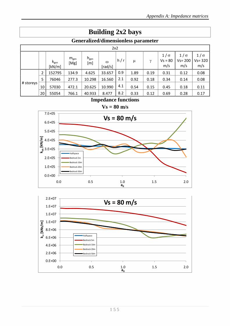
Appendix A: Impedance matrices
1 5 5
Building 2x2 bays
Generalized/dimensionless parameter
2x2
kgen
[kN/m]
mgen [Mg]
hgen [m]
[rad/s]
h / r 1 / Vs = 80
m/s
1 / Vs= 200
m/s
1 / Vs= 320
m/s
# storeys
2 152795 134.9 4.625 33.657 0.9 1.89 0.19 0.31 0.12 0.08
5 76046 277.3 10.298 16.560 2.1 0.92 0.18 0.34 0.14 0.08
10 57030 472.1 20.625 10.990 4.1 0.54 0.15 0.45 0.18 0.11
20 55054 766.1 40.933 8.477 8.2 0.33 0.12 0.69 0.28 0.17
Impedance functions
Vs = 80 m/s
0.E+00
1.E+05
2.E+05
3.E+05
4.E+05
5.E+05
6.E+05
7.E+05
0.0 0.5 1.0 1.5 2.0
k hh
[kN
/m]
a0
Vs = 80 m/s
Halfspace
Bedrock 5m
Bedrock 10m
Bedrock 20m
Bedrock 50m
0.E+00
2.E+06
4.E+06
6.E+06
8.E+06
1.E+07
1.E+07
1.E+07
2.E+07
0.0 0.5 1.0 1.5 2.0
k rr[k
Ns/
m]
a0
Vs = 80 m/s
Halfspace
Bedrock 5m
Bedrock 10m
Bedrock 20m
Bedrock 50m
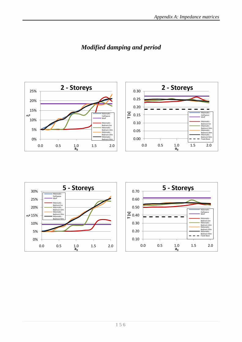
Appendix A: Impedance matrices
1 5 6
Modified damping and period
0%
5%
10%
15%
20%
25%
0.0 0.5 1.0 1.5 2.0
a0
2 - Storeys
Mylonakis -HalfspaceWolf
Mylonakis -Bedrock 5mMylonakis -Bedrock 10mMylonakis -Bedrock 20mMylonakis -Bedrock 50m 0.00
0.05
0.10
0.15
0.20
0.25
0.30
0.0 0.5 1.0 1.5 2.0
T [s
]
a0
2 - Storeys
Mylonakis -HalfspaceWolf
Mylonakis -Bedrock 5mMylonakis -Bedrock 10mMylonakis -Bedrock 20mMylonakis -Bedrock 50mFixed-Base
0%
5%
10%
15%
20%
25%
30%
0.0 0.5 1.0 1.5 2.0
a0
5 - StoreysMylonakis -HalfspaceWolf
Mylonakis -Bedrock 5mMylonakis -Bedrock 10mMylonakis -Bedrock 20mMylonakis -Bedrock 50m
0.10
0.20
0.30
0.40
0.50
0.60
0.70
0.0 0.5 1.0 1.5 2.0
T [s
]
a0
5 - Storeys
Mylonakis -HalfspaceWolf
Mylonakis -Bedrock 5mMylonakis -Bedrock 10mMylonakis -Bedrock 20mMylonakis -Bedrock 50mFixed-Base
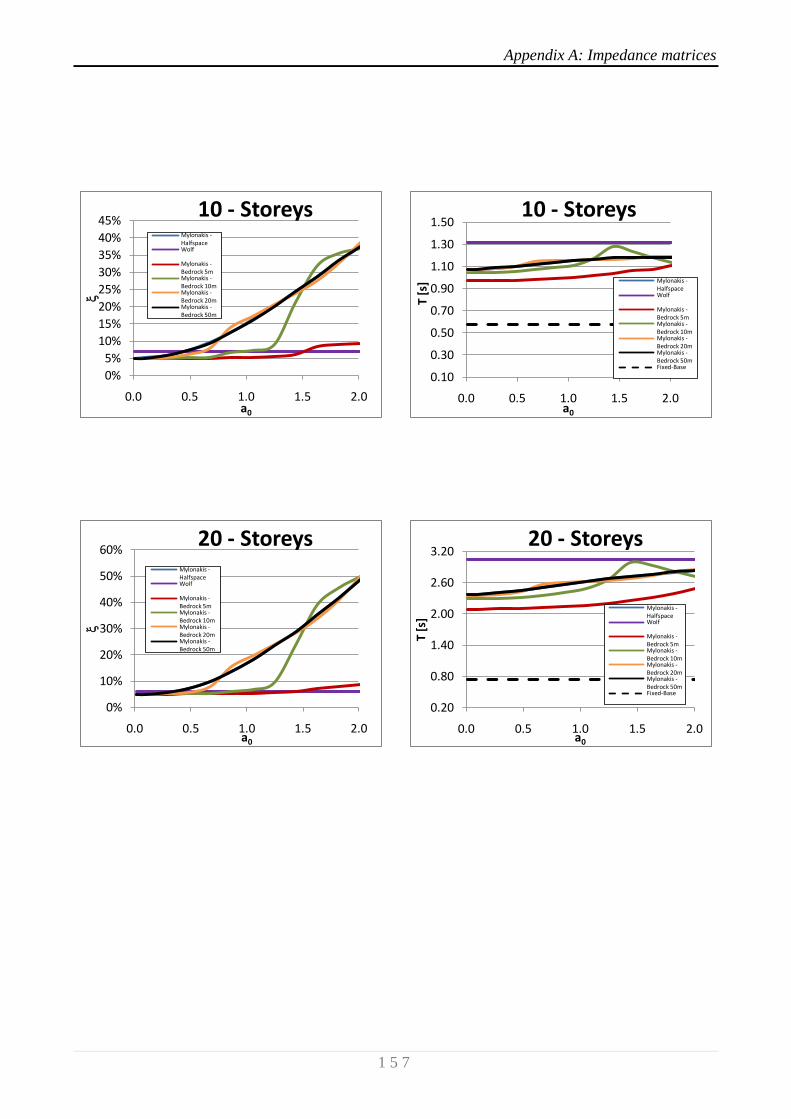
Appendix A: Impedance matrices
1 5 7
0%
5%
10%
15%
20%
25%
30%
35%
40%
45%
0.0 0.5 1.0 1.5 2.0
a0
10 - StoreysMylonakis -HalfspaceWolf
Mylonakis -Bedrock 5mMylonakis -Bedrock 10mMylonakis -Bedrock 20mMylonakis -Bedrock 50m
0.10
0.30
0.50
0.70
0.90
1.10
1.30
1.50
0.0 0.5 1.0 1.5 2.0
T [s
]a0
10 - Storeys
Mylonakis -HalfspaceWolf
Mylonakis -Bedrock 5mMylonakis -Bedrock 10mMylonakis -Bedrock 20mMylonakis -Bedrock 50mFixed-Base
0%
10%
20%
30%
40%
50%
60%
0.0 0.5 1.0 1.5 2.0
a0
20 - StoreysMylonakis -HalfspaceWolf
Mylonakis -Bedrock 5mMylonakis -Bedrock 10mMylonakis -Bedrock 20mMylonakis -Bedrock 50m
0.20
0.80
1.40
2.00
2.60
3.20
0.0 0.5 1.0 1.5 2.0
T [s
]
a0
20 - Storeys
Mylonakis -HalfspaceWolf
Mylonakis -Bedrock 5mMylonakis -Bedrock 10mMylonakis -Bedrock 20mMylonakis -Bedrock 50mFixed-Base
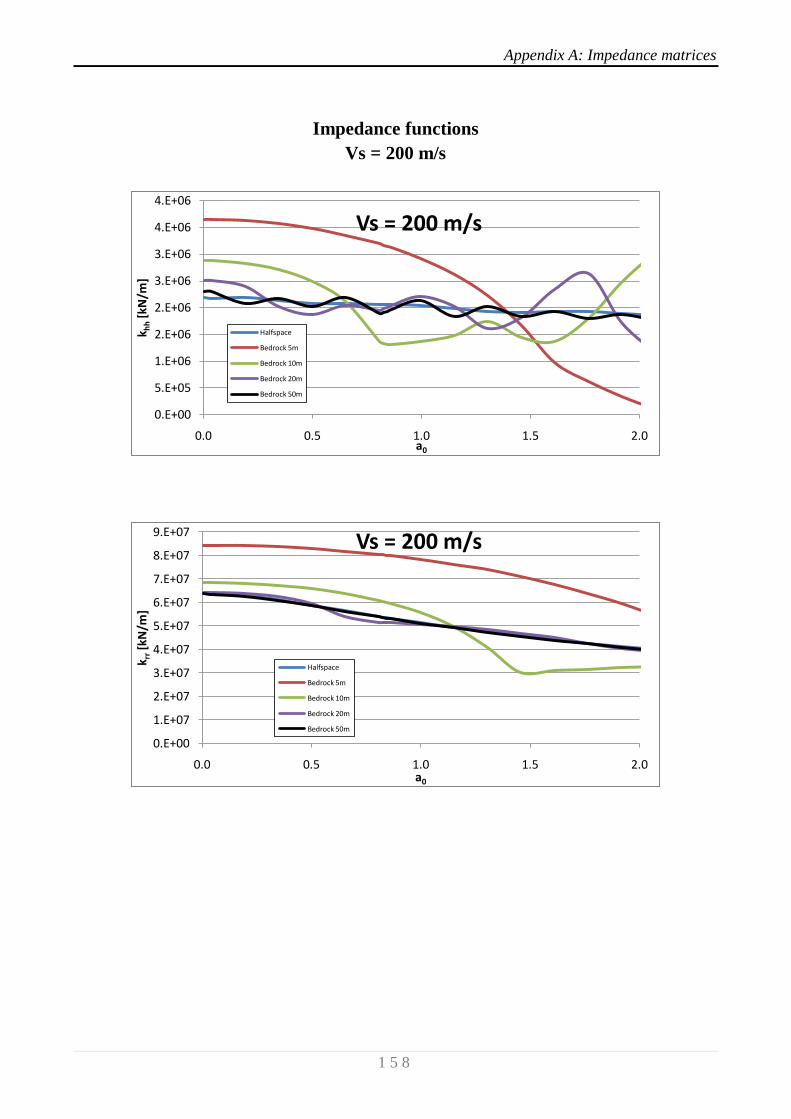
Appendix A: Impedance matrices
1 5 8
Impedance functions
Vs = 200 m/s
0.E+00
5.E+05
1.E+06
2.E+06
2.E+06
3.E+06
3.E+06
4.E+06
4.E+06
0.0 0.5 1.0 1.5 2.0
k hh
[kN
/m]
a0
Vs = 200 m/s
Halfspace
Bedrock 5m
Bedrock 10m
Bedrock 20m
Bedrock 50m
0.E+00
1.E+07
2.E+07
3.E+07
4.E+07
5.E+07
6.E+07
7.E+07
8.E+07
9.E+07
0.0 0.5 1.0 1.5 2.0
k rr[k
N/m
]
a0
Vs = 200 m/s
Halfspace
Bedrock 5m
Bedrock 10m
Bedrock 20m
Bedrock 50m
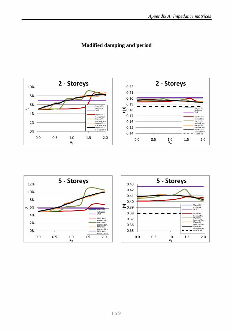
Appendix A: Impedance matrices
1 5 9
Modified damping and period
0%
2%
4%
6%
8%
10%
0.0 0.5 1.0 1.5 2.0
a0
2 - Storeys
Mylonakis -HalfspaceWolf
Mylonakis -Bedrock 5mMylonakis -Bedrock 10mMylonakis -Bedrock 20mMylonakis -Bedrock 50m
0.14
0.15
0.16
0.17
0.18
0.19
0.20
0.21
0.22
0.0 0.5 1.0 1.5 2.0
T [s
]
a0
2 - Storeys
Mylonakis -HalfspaceWolf
Mylonakis -Bedrock 5mMylonakis -Bedrock 10mMylonakis -Bedrock 20mMylonakis -Bedrock 50mFixed-Base
0%
2%
4%
6%
8%
10%
12%
0.0 0.5 1.0 1.5 2.0
a0
5 - Storeys
Mylonakis -HalfspaceWolf
Mylonakis -Bedrock 5mMylonakis -Bedrock 10mMylonakis -Bedrock 20mMylonakis -Bedrock 50m
0.35
0.36
0.37
0.38
0.39
0.40
0.41
0.42
0.43
0.0 0.5 1.0 1.5 2.0
T [s
]
a0
5 - Storeys
Mylonakis -HalfspaceWolf
Mylonakis -Bedrock 5mMylonakis -Bedrock 10mMylonakis -Bedrock 20mMylonakis -Bedrock 50mFixed-Base
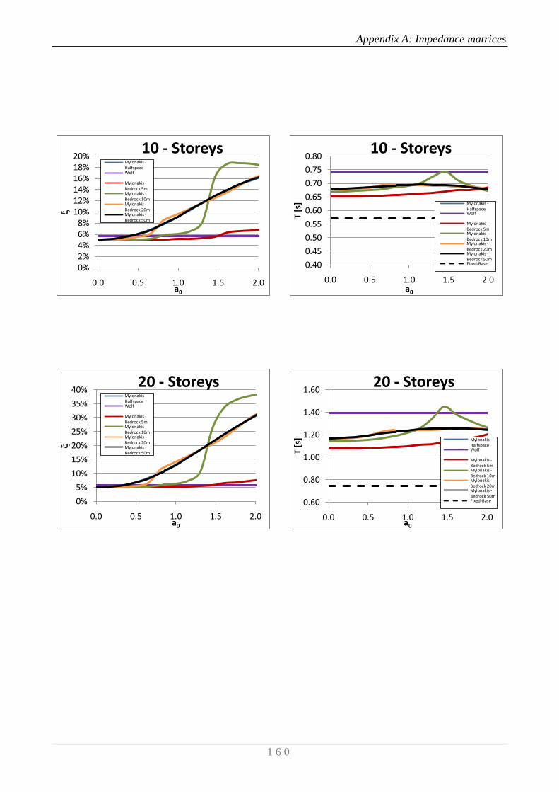
Appendix A: Impedance matrices
1 6 0
0%2%4%6%8%
10%12%14%16%18%20%
0.0 0.5 1.0 1.5 2.0
a0
10 - StoreysMylonakis -HalfspaceWolf
Mylonakis -Bedrock 5mMylonakis -Bedrock 10mMylonakis -Bedrock 20mMylonakis -Bedrock 50m
0.40
0.45
0.50
0.55
0.60
0.65
0.70
0.75
0.80
0.0 0.5 1.0 1.5 2.0
T [s
]a0
10 - Storeys
Mylonakis -HalfspaceWolf
Mylonakis -Bedrock 5mMylonakis -Bedrock 10mMylonakis -Bedrock 20mMylonakis -Bedrock 50mFixed-Base
0%
5%
10%
15%
20%
25%
30%
35%
40%
0.0 0.5 1.0 1.5 2.0
a0
20 - StoreysMylonakis -HalfspaceWolf
Mylonakis -Bedrock 5mMylonakis -Bedrock 10mMylonakis -Bedrock 20mMylonakis -Bedrock 50m
0.60
0.80
1.00
1.20
1.40
1.60
0.0 0.5 1.0 1.5 2.0
T [
s]
a0
20 - Storeys
Mylonakis -HalfspaceWolf
Mylonakis -Bedrock 5mMylonakis -Bedrock 10mMylonakis -Bedrock 20mMylonakis -Bedrock 50mFixed-Base
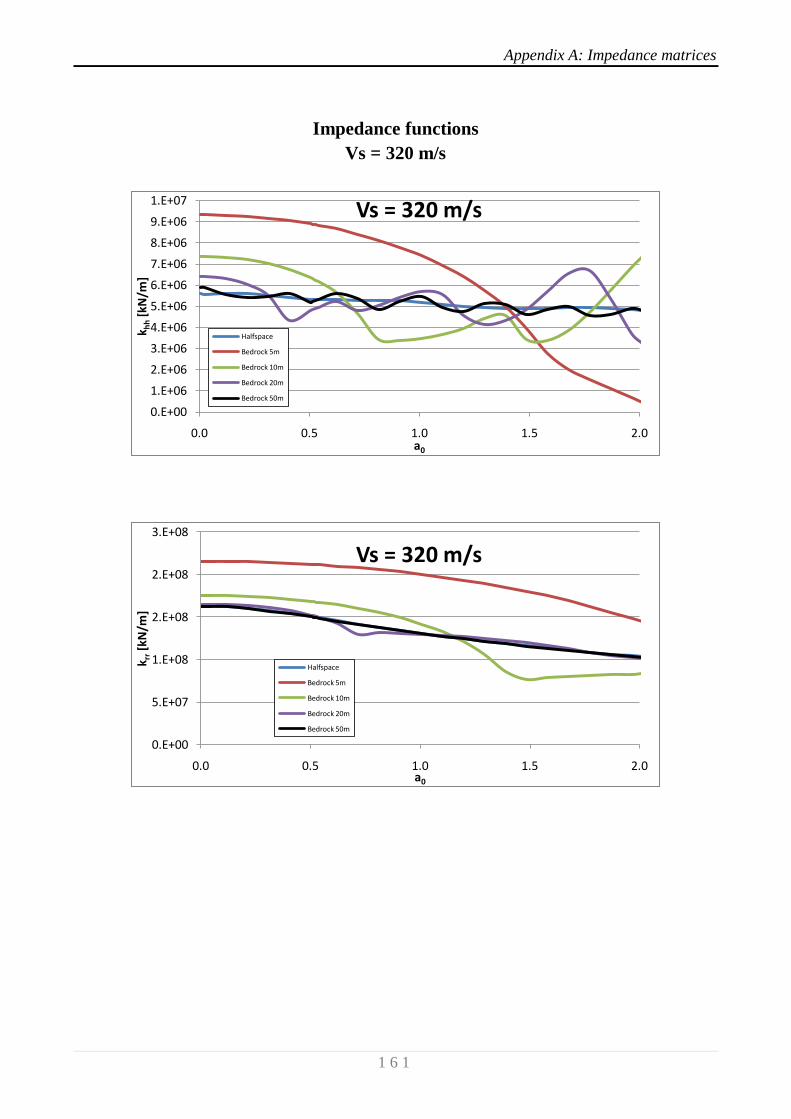
Appendix A: Impedance matrices
1 6 1
Impedance functions
Vs = 320 m/s
0.E+00
1.E+06
2.E+06
3.E+06
4.E+06
5.E+06
6.E+06
7.E+06
8.E+06
9.E+06
1.E+07
0.0 0.5 1.0 1.5 2.0
k hh
[kN
/m]
a0
Vs = 320 m/s
Halfspace
Bedrock 5m
Bedrock 10m
Bedrock 20m
Bedrock 50m
0.E+00
5.E+07
1.E+08
2.E+08
2.E+08
3.E+08
0.0 0.5 1.0 1.5 2.0
k rr[k
N/m
]
a0
Vs = 320 m/s
Halfspace
Bedrock 5m
Bedrock 10m
Bedrock 20m
Bedrock 50m

Appendix A: Impedance matrices
1 6 2
Modified damping and period
0%
1%
2%
3%
4%
5%
6%
7%
8%
0.0 0.5 1.0 1.5 2.0
a0
2 - Storeys
Mylonakis -HalfspaceWolf
Mylonakis -Bedrock 5mMylonakis -Bedrock 10mMylonakis -Bedrock 20mMylonakis -Bedrock 50m
0.15
0.16
0.17
0.18
0.19
0.20
0.0 0.5 1.0 1.5 2.0
T [s
]
a0
2 - Storeys
Mylonakis -HalfspaceWolf
Mylonakis -Bedrock 5mMylonakis -Bedrock 10mMylonakis -Bedrock 20mMylonakis -Bedrock 50mFixed-Base
4%
5%
6%
7%
8%
0.0 0.5 1.0 1.5 2.0
a0
5 - StoreysMylonakis -HalfspaceWolf
Mylonakis -Bedrock 5mMylonakis -Bedrock 10mMylonakis -Bedrock 20mMylonakis -Bedrock 50m
0.35
0.36
0.37
0.38
0.39
0.40
0.0 0.5 1.0 1.5 2.0
T [s
]
a0
5 - Storeys
Mylonakis -HalfspaceWolf
Mylonakis -Bedrock 5mMylonakis -Bedrock 10mMylonakis -Bedrock 20mMylonakis -Bedrock 50mFixed-Base

Appendix A: Impedance matrices
1 6 3
4%
5%
6%
7%
8%
9%
10%
11%
12%
0.0 0.5 1.0 1.5 2.0
a0
10 - StoreysMylonakis -HalfspaceWolf
Mylonakis -Bedrock 5mMylonakis -Bedrock 10mMylonakis -Bedrock 20mMylonakis -Bedrock 50m
0.40
0.45
0.50
0.55
0.60
0.65
0.70
0.0 0.5 1.0 1.5 2.0
T [s
]a0
10 - Storeys
Mylonakis -HalfspaceWolf
Mylonakis -Bedrock 5mMylonakis -Bedrock 10mMylonakis -Bedrock 20mMylonakis -Bedrock 50mFixed-Base
4%
9%
14%
19%
24%
0.0 0.5 1.0 1.5 2.0
a0
20 - StoreysMylonakis -HalfspaceWolf
Mylonakis -Bedrock 5mMylonakis -Bedrock 10mMylonakis -Bedrock 20mMylonakis -Bedrock 50m
0.60
0.70
0.80
0.90
1.00
1.10
0.0 0.5 1.0 1.5 2.0
T [
s]
a0
20 - Storeys
Mylonakis -HalfspaceWolf
Mylonakis -Bedrock 5mMylonakis -Bedrock 10mMylonakis -Bedrock 20mMylonakis -Bedrock 50mFixed-Base
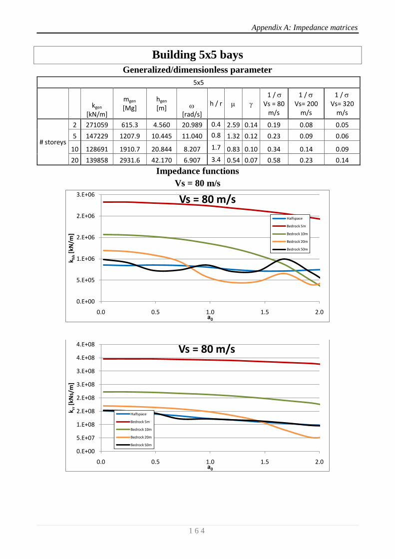
Appendix A: Impedance matrices
1 6 4
Building 5x5 bays
Generalized/dimensionless parameter
5x5
kgen
[kN/m]
mgen [Mg]
hgen [m]
[rad/s]
h / r 1 / Vs = 80
m/s
1 / Vs= 200
m/s
1 / Vs= 320
m/s
# storeys
2 271059 615.3 4.560 20.989 0.4 2.59 0.14 0.19 0.08 0.05
5 147229 1207.9 10.445 11.040 0.8 1.32 0.12 0.23 0.09 0.06
10 128691 1910.7 20.844 8.207 1.7 0.83 0.10 0.34 0.14 0.09
20 139858 2931.6 42.170 6.907 3.4 0.54 0.07 0.58 0.23 0.14
Impedance functions
Vs = 80 m/s
0.E+00
5.E+05
1.E+06
2.E+06
2.E+06
3.E+06
0.0 0.5 1.0 1.5 2.0
k hh
[kN
/m]
a0
Vs = 80 m/s
Halfspace
Bedrock 5m
Bedrock 10m
Bedrock 20m
Bedrock 50m
0.E+00
5.E+07
1.E+08
2.E+08
2.E+08
3.E+08
3.E+08
4.E+08
4.E+08
0.0 0.5 1.0 1.5 2.0
k rr[k
Ns/
m]
a0
Vs = 80 m/s
Halfspace
Bedrock 5m
Bedrock 10m
Bedrock 20m
Bedrock 50m
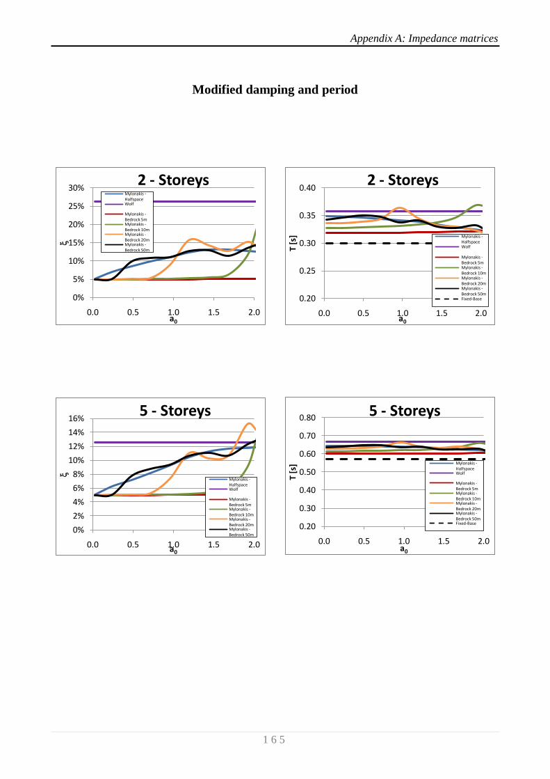
Appendix A: Impedance matrices
1 6 5
Modified damping and period
0%
5%
10%
15%
20%
25%
30%
0.0 0.5 1.0 1.5 2.0
a0
2 - StoreysMylonakis -HalfspaceWolf
Mylonakis -Bedrock 5mMylonakis -Bedrock 10mMylonakis -Bedrock 20mMylonakis -Bedrock 50m
0.20
0.25
0.30
0.35
0.40
0.0 0.5 1.0 1.5 2.0
T [s
]
a0
2 - Storeys
Mylonakis -HalfspaceWolf
Mylonakis -Bedrock 5mMylonakis -Bedrock 10mMylonakis -Bedrock 20mMylonakis -Bedrock 50mFixed-Base
0%
2%
4%
6%
8%
10%
12%
14%
16%
0.0 0.5 1.0 1.5 2.0
a0
5 - Storeys
Mylonakis -HalfspaceWolf
Mylonakis -Bedrock 5mMylonakis -Bedrock 10mMylonakis -Bedrock 20mMylonakis -Bedrock 50m
0.20
0.30
0.40
0.50
0.60
0.70
0.80
0.0 0.5 1.0 1.5 2.0
T [s
]
a0
5 - Storeys
Mylonakis -HalfspaceWolf
Mylonakis -Bedrock 5mMylonakis -Bedrock 10mMylonakis -Bedrock 20mMylonakis -Bedrock 50mFixed-Base
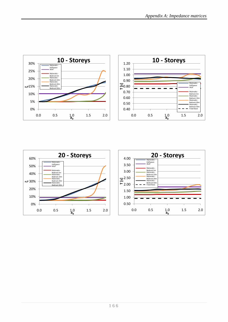
Appendix A: Impedance matrices
1 6 6
0%
5%
10%
15%
20%
25%
30%
0.0 0.5 1.0 1.5 2.0
a0
10 - StoreysMylonakis -HalfspaceWolf
Mylonakis -Bedrock 5mMylonakis -Bedrock 10mMylonakis -Bedrock 20mMylonakis -Bedrock 50m
0.40
0.50
0.60
0.70
0.80
0.90
1.00
1.10
1.20
0.0 0.5 1.0 1.5 2.0
T [s
]a0
10 - Storeys
Mylonakis -HalfspaceWolf
Mylonakis -Bedrock 5mMylonakis -Bedrock 10mMylonakis -Bedrock 20mMylonakis -Bedrock 50mFixed-Base
0%
10%
20%
30%
40%
50%
60%
0.0 0.5 1.0 1.5 2.0
a0
20 - StoreysMylonakis -HalfspaceWolf
Mylonakis -Bedrock 5mMylonakis -Bedrock 10mMylonakis -Bedrock 20mMylonakis -Bedrock 50m
0.50
1.00
1.50
2.00
2.50
3.00
3.50
4.00
0.0 0.5 1.0 1.5 2.0
T [
s]
a0
20 - StoreysMylonakis -HalfspaceWolf
Mylonakis -Bedrock 5mMylonakis -Bedrock 10mMylonakis -Bedrock 20mMylonakis -Bedrock 50mFixed-Base
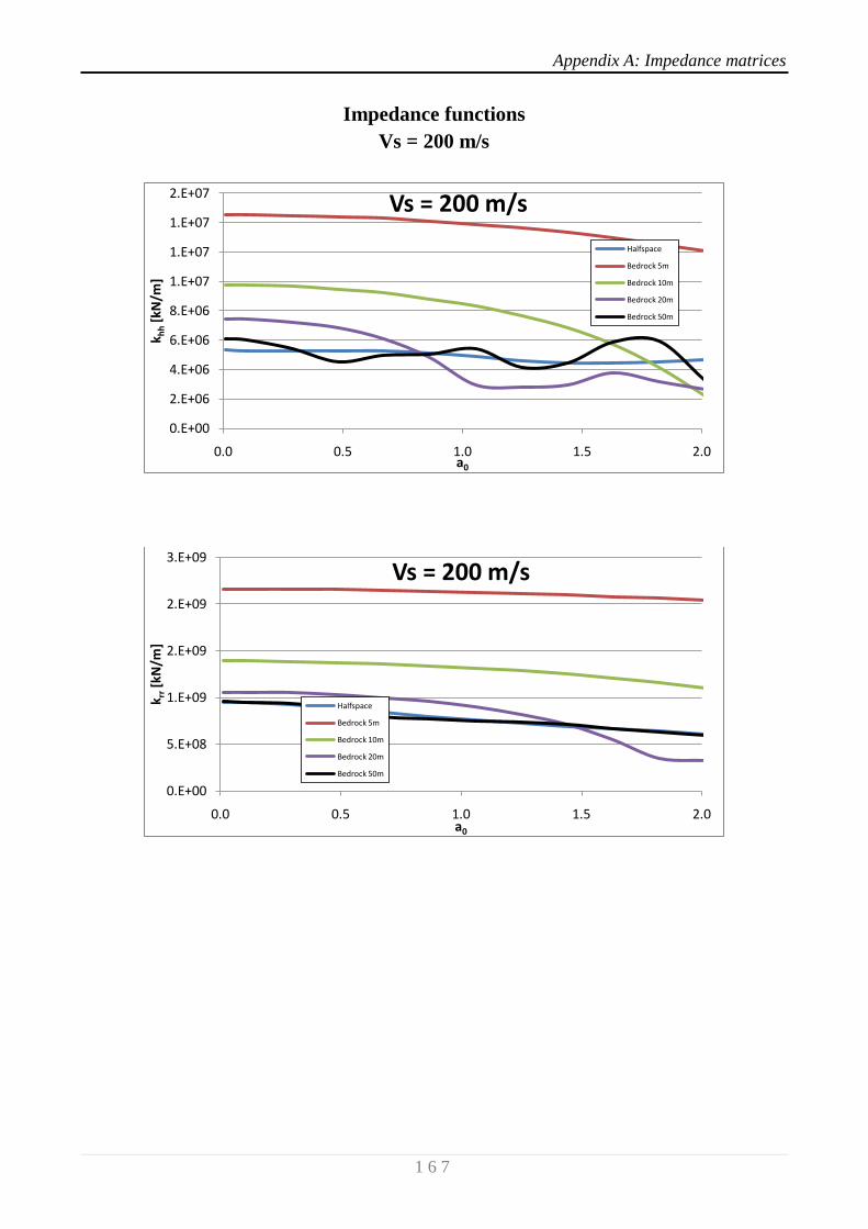
Appendix A: Impedance matrices
1 6 7
Impedance functions
Vs = 200 m/s
0.E+00
2.E+06
4.E+06
6.E+06
8.E+06
1.E+07
1.E+07
1.E+07
2.E+07
0.0 0.5 1.0 1.5 2.0
k hh
[kN
/m]
a0
Vs = 200 m/s
Halfspace
Bedrock 5m
Bedrock 10m
Bedrock 20m
Bedrock 50m
0.E+00
5.E+08
1.E+09
2.E+09
2.E+09
3.E+09
0.0 0.5 1.0 1.5 2.0
k rr[k
N/m
]
a0
Vs = 200 m/s
Halfspace
Bedrock 5m
Bedrock 10m
Bedrock 20m
Bedrock 50m
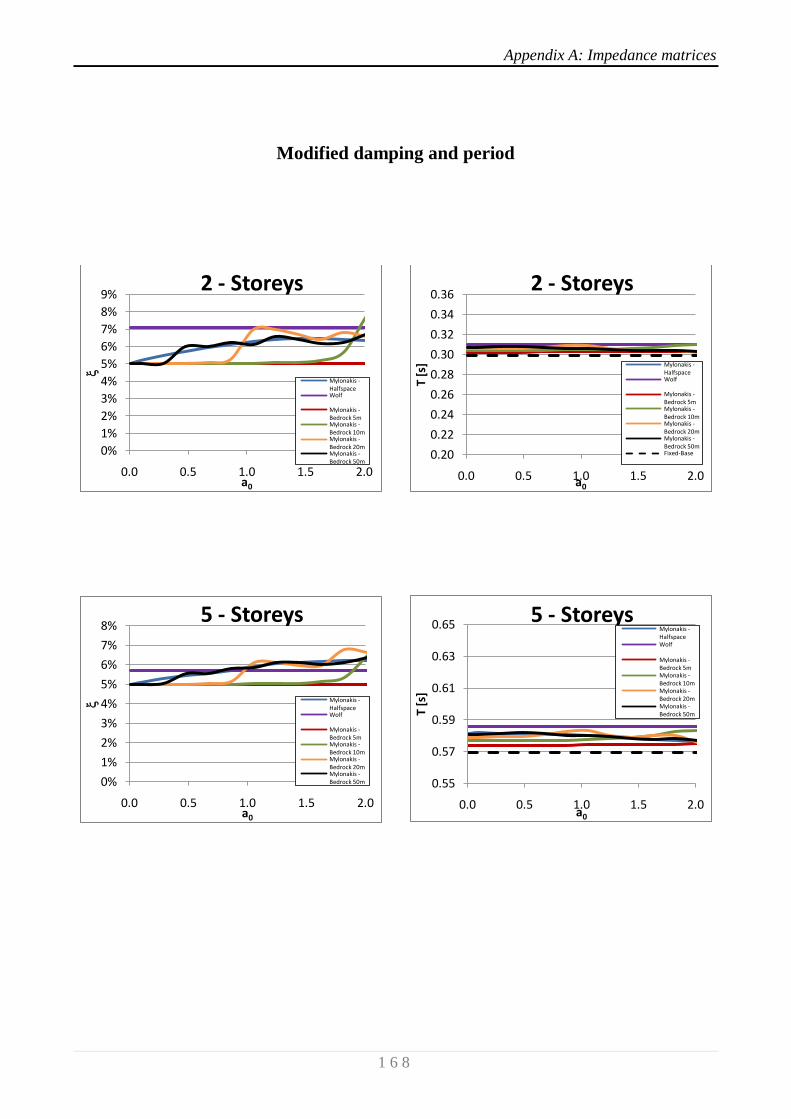
Appendix A: Impedance matrices
1 6 8
Modified damping and period
0%
1%
2%
3%
4%
5%
6%
7%
8%
9%
0.0 0.5 1.0 1.5 2.0
a0
2 - Storeys
Mylonakis -HalfspaceWolf
Mylonakis -Bedrock 5mMylonakis -Bedrock 10mMylonakis -Bedrock 20mMylonakis -Bedrock 50m
0.20
0.22
0.24
0.26
0.28
0.30
0.32
0.34
0.36
0.0 0.5 1.0 1.5 2.0
T [s
]
a0
2 - Storeys
Mylonakis -HalfspaceWolf
Mylonakis -Bedrock 5mMylonakis -Bedrock 10mMylonakis -Bedrock 20mMylonakis -Bedrock 50mFixed-Base
0%
1%
2%
3%
4%
5%
6%
7%
8%
0.0 0.5 1.0 1.5 2.0
a0
5 - Storeys
Mylonakis -HalfspaceWolf
Mylonakis -Bedrock 5mMylonakis -Bedrock 10mMylonakis -Bedrock 20mMylonakis -Bedrock 50m 0.55
0.57
0.59
0.61
0.63
0.65
0.0 0.5 1.0 1.5 2.0
T [s
]
a0
5 - StoreysMylonakis -HalfspaceWolf
Mylonakis -Bedrock 5mMylonakis -Bedrock 10mMylonakis -Bedrock 20mMylonakis -Bedrock 50m

Appendix A: Impedance matrices
1 6 9
0%1%2%3%4%5%6%7%8%9%
10%
0.0 0.5 1.0 1.5 2.0
a0
10 - Storeys
Mylonakis -HalfspaceWolf
Mylonakis -Bedrock 5mMylonakis -Bedrock 10mMylonakis -Bedrock 20mMylonakis -Bedrock 50m
0.70
0.72
0.74
0.76
0.78
0.80
0.82
0.84
0.0 0.5 1.0 1.5 2.0
T [s
]a0
10 - Storeys
Mylonakis -HalfspaceWolf
Mylonakis -Bedrock 5mMylonakis -Bedrock 10mMylonakis -Bedrock 20mMylonakis -Bedrock 50mFixed-Base
0%
5%
10%
15%
20%
0.0 0.5 1.0 1.5 2.0
a0
20 - StoreysMylonakis -HalfspaceWolf
Mylonakis -Bedrock 5mMylonakis -Bedrock 10mMylonakis -Bedrock 20mMylonakis -Bedrock 50m
0.60
0.80
1.00
1.20
1.40
1.60
1.80
2.00
0.0 0.5 1.0 1.5 2.0
T [s
]
a0
20 - StoreysMylonakis -HalfspaceWolf
Mylonakis -Bedrock 5mMylonakis -Bedrock 10mMylonakis -Bedrock 20mMylonakis -Bedrock 50mFixed-Base
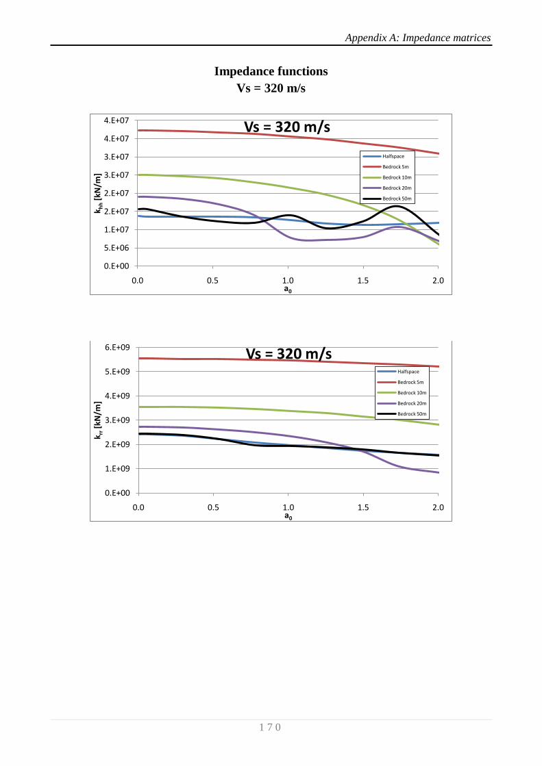
Appendix A: Impedance matrices
1 7 0
Impedance functions
Vs = 320 m/s
0.E+00
5.E+06
1.E+07
2.E+07
2.E+07
3.E+07
3.E+07
4.E+07
4.E+07
0.0 0.5 1.0 1.5 2.0
k hh
[kN
/m]
a0
Vs = 320 m/s
Halfspace
Bedrock 5m
Bedrock 10m
Bedrock 20m
Bedrock 50m
0.E+00
1.E+09
2.E+09
3.E+09
4.E+09
5.E+09
6.E+09
0.0 0.5 1.0 1.5 2.0
k rr[k
N/m
]
a0
Vs = 320 m/sHalfspace
Bedrock 5m
Bedrock 10m
Bedrock 20m
Bedrock 50m

Appendix A: Impedance matrices
1 7 1
Modified damping and period
0%
1%
2%
3%
4%
5%
6%
7%
0.0 0.5 1.0 1.5 2.0
a0
2 - Storeys
Mylonakis -HalfspaceWolf
Mylonakis -Bedrock 5mMylonakis -Bedrock 10mMylonakis -Bedrock 20mMylonakis -Bedrock 50m
0.20
0.22
0.24
0.26
0.28
0.30
0.32
0.34
0.0 0.5 1.0 1.5 2.0
T [s
]
a0
2 - Storeys
Mylonakis -HalfspaceWolf
Mylonakis -Bedrock 5mMylonakis -Bedrock 10mMylonakis -Bedrock 20mMylonakis -Bedrock 50mFixed-Base
2%
3%
4%
5%
6%
7%
8%
9%
10%
0.0 0.5 1.0 1.5 2.0
a0
5 - StoreysMylonakis -HalfspaceWolf
Mylonakis -Bedrock 5mMylonakis -Bedrock 10mMylonakis -Bedrock 20mMylonakis -Bedrock 50m
0.50
0.52
0.54
0.56
0.58
0.60
0.0 0.5 1.0 1.5 2.0
T [s
]
a0
5 - Storeys
Mylonakis -HalfspaceWolf
Mylonakis -Bedrock 5mMylonakis -Bedrock 10mMylonakis -Bedrock 20mMylonakis -Bedrock 50mFixed-Base
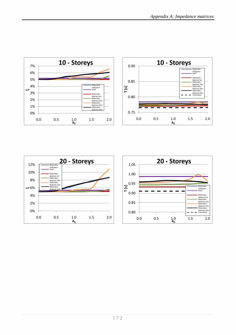
Appendix A: Impedance matrices
1 7 2
0%
1%
2%
3%
4%
5%
6%
7%
0.0 0.5 1.0 1.5 2.0
a0
10 - Storeys
Mylonakis -HalfspaceWolf
Mylonakis -Bedrock 5mMylonakis -Bedrock 10mMylonakis -Bedrock 20mMylonakis -Bedrock 50m
0.75
0.80
0.85
0.90
0.0 0.5 1.0 1.5 2.0
T [s
]a0
10 - StoreysMylonakis -HalfspaceWolf
Mylonakis -Bedrock 5mMylonakis -Bedrock 10mMylonakis -Bedrock 20mMylonakis -Bedrock 50mFixed-Base
0%
2%
4%
6%
8%
10%
12%
0.0 0.5 1.0 1.5 2.0
a0
20 - StoreysMylonakis -HalfspaceWolf
Mylonakis -Bedrock 5mMylonakis -Bedrock 10mMylonakis -Bedrock 20mMylonakis -Bedrock 50m
0.80
0.85
0.90
0.95
1.00
1.05
0.0 0.5 1.0 1.5 2.0
T [s
]
a0
20 - Storeys
Mylonakis -HalfspaceWolf
Mylonakis -Bedrock 5mMylonakis -Bedrock 10mMylonakis -Bedrock 20mMylonakis -Bedrock 50mFixed-Base

Appendix A: Impedance matrices
1 7 3
Building 10x10 bays
Generalized/dimensionless parameter
10x10
kgen
[kN/m]
mgen [Mg]
hgen [m]
[rad/s]
h / r 1 / Vs = 80
m/s
1 / Vs= 200
m/s
1 / Vs= 320
m/s
# storeys
2 641806 2163.4 4.525 17.224 0.2 2.94 0.13 0.16 0.06 0.04
5 363980 4130.6 10.537 9.387 0.4 1.54 0.10 0.20 0.08 0.05
10 339265 6298.7 21.125 7.339 0.8 1.01 0.08 0.31 0.12 0.08
20 385518 9453.4 42.681 6.386 1.7 0.67 0.06 0.54 0.22 0.14
Impedance functions
Vs = 80 m/s
0.E+00
1.E+06
2.E+06
3.E+06
4.E+06
5.E+06
6.E+06
7.E+06
8.E+06
0.0 0.5 1.0 1.5 2.0
k hh
[kN
/m]
a0
Vs = 80 m/sHalfspace
Bedrock 5m
Bedrock 10m
Bedrock 20m
Bedrock 50m
0.E+00
5.E+08
1.E+09
2.E+09
2.E+09
3.E+09
3.E+09
4.E+09
4.E+09
5.E+09
5.E+09
0.0 0.5 1.0 1.5 2.0
k rr[k
Ns/
m]
a0
Vs = 80 m/sHalfspace
Bedrock 5m
Bedrock 10m
Bedrock 20m
Bedrock 50m
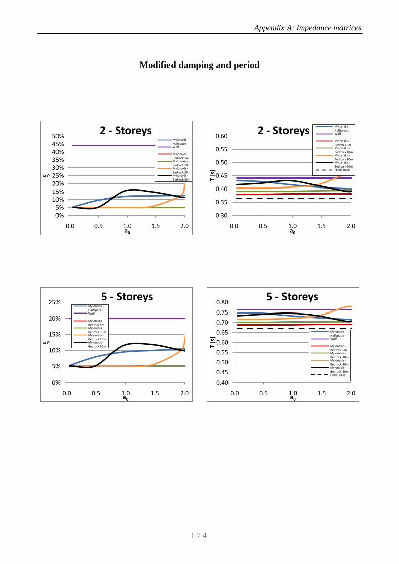
Appendix A: Impedance matrices
1 7 4
Modified damping and period
0%5%
10%15%20%25%30%35%40%45%50%
0.0 0.5 1.0 1.5 2.0
a0
2 - StoreysMylonakis -HalfspaceWolf
Mylonakis -Bedrock 5mMylonakis -Bedrock 10mMylonakis -Bedrock 20mMylonakis -Bedrock 50m
0.30
0.35
0.40
0.45
0.50
0.55
0.60
0.0 0.5 1.0 1.5 2.0
T [s
]
a0
2 - StoreysMylonakis -HalfspaceWolf
Mylonakis -Bedrock 5mMylonakis -Bedrock 10mMylonakis -Bedrock 20mMylonakis -Bedrock 50mFixed-Base
0%
5%
10%
15%
20%
25%
0.0 0.5 1.0 1.5 2.0
a0
5 - StoreysMylonakis -HalfspaceWolf
Mylonakis -Bedrock 5mMylonakis -Bedrock 10mMylonakis -Bedrock 20mMylonakis -Bedrock 50m
0.40
0.45
0.50
0.55
0.60
0.65
0.70
0.75
0.80
0.0 0.5 1.0 1.5 2.0
T [s
]
a0
5 - Storeys
Mylonakis -HalfspaceWolf
Mylonakis -Bedrock 5mMylonakis -Bedrock 10mMylonakis -Bedrock 20mMylonakis -Bedrock 50mFixed-Base
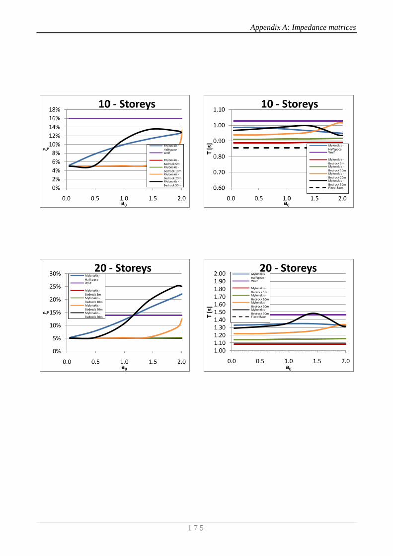
Appendix A: Impedance matrices
1 7 5
0%
2%
4%
6%
8%
10%
12%
14%
16%
18%
0.0 0.5 1.0 1.5 2.0
a0
10 - Storeys
Mylonakis -HalfspaceWolf
Mylonakis -Bedrock 5mMylonakis -Bedrock 10mMylonakis -Bedrock 20mMylonakis -Bedrock 50m
0.60
0.70
0.80
0.90
1.00
1.10
0.0 0.5 1.0 1.5 2.0
T [s
]a0
10 - Storeys
Mylonakis -HalfspaceWolf
Mylonakis -Bedrock 5mMylonakis -Bedrock 10mMylonakis -Bedrock 20mMylonakis -Bedrock 50mFixed-Base
0%
5%
10%
15%
20%
25%
30%
0.0 0.5 1.0 1.5 2.0
a0
20 - StoreysMylonakis -HalfspaceWolf
Mylonakis -Bedrock 5mMylonakis -Bedrock 10mMylonakis -Bedrock 20mMylonakis -Bedrock 50m
1.001.101.201.301.401.501.601.701.801.902.00
0.0 0.5 1.0 1.5 2.0
T [
s]
a0
20 - StoreysMylonakis -HalfspaceWolf
Mylonakis -Bedrock 5mMylonakis -Bedrock 10mMylonakis -Bedrock 20mMylonakis -Bedrock 50mFixed-Base
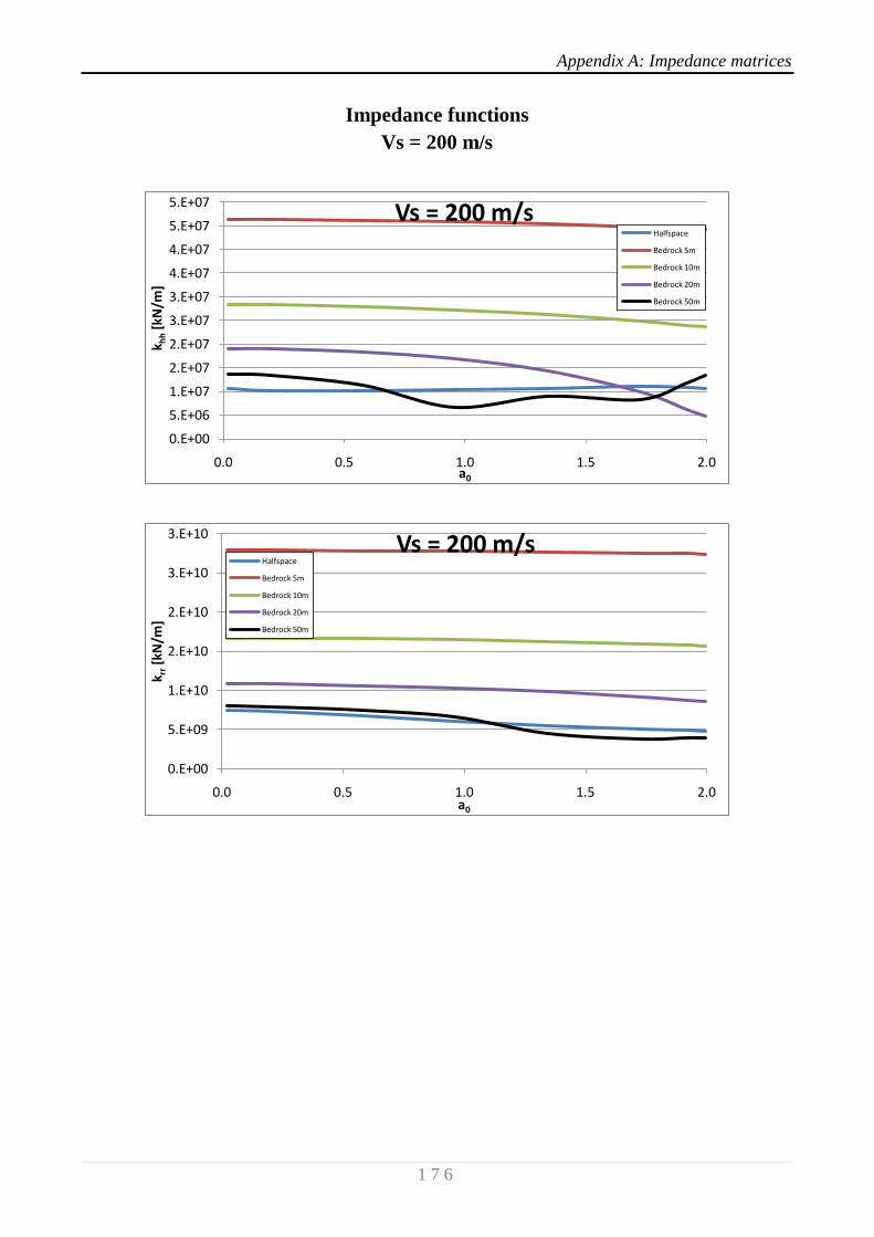
Appendix A: Impedance matrices
1 7 6
Impedance functions
Vs = 200 m/s
0.E+00
5.E+06
1.E+07
2.E+07
2.E+07
3.E+07
3.E+07
4.E+07
4.E+07
5.E+07
5.E+07
0.0 0.5 1.0 1.5 2.0
k hh
[kN
/m]
a0
Vs = 200 m/sHalfspace
Bedrock 5m
Bedrock 10m
Bedrock 20m
Bedrock 50m
0.E+00
5.E+09
1.E+10
2.E+10
2.E+10
3.E+10
3.E+10
0.0 0.5 1.0 1.5 2.0
k rr[k
N/m
]
a0
Vs = 200 m/sHalfspace
Bedrock 5m
Bedrock 10m
Bedrock 20m
Bedrock 50m
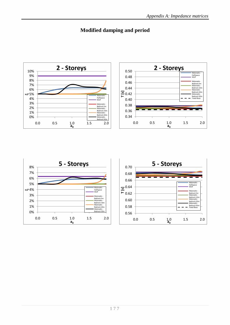
Appendix A: Impedance matrices
1 7 7
Modified damping and period
0%1%2%3%4%5%6%7%8%9%
10%
0.0 0.5 1.0 1.5 2.0
a0
2 - Storeys
Mylonakis -HalfspaceWolf
Mylonakis -Bedrock 5mMylonakis -Bedrock 10mMylonakis -Bedrock 20mMylonakis -Bedrock 50m
0.34
0.36
0.38
0.40
0.42
0.44
0.46
0.48
0.50
0.0 0.5 1.0 1.5 2.0T
[s]
a0
2 - StoreysMylonakis -HalfspaceWolf
Mylonakis -Bedrock 5mMylonakis -Bedrock 10mMylonakis -Bedrock 20mMylonakis -Bedrock 50mFixed-Base
0%
1%
2%
3%
4%
5%
6%
7%
8%
0.0 0.5 1.0 1.5 2.0
a0
5 - Storeys
Mylonakis -HalfspaceWolf
Mylonakis -Bedrock 5mMylonakis -Bedrock 10mMylonakis -Bedrock 20mMylonakis -Bedrock 50m
0.56
0.58
0.60
0.62
0.64
0.66
0.68
0.70
0.0 0.5 1.0 1.5 2.0
T [s
]
a0
5 - Storeys
Mylonakis -HalfspaceWolf
Mylonakis -Bedrock 5mMylonakis -Bedrock 10mMylonakis -Bedrock 20mMylonakis -Bedrock 50mFixed-Base
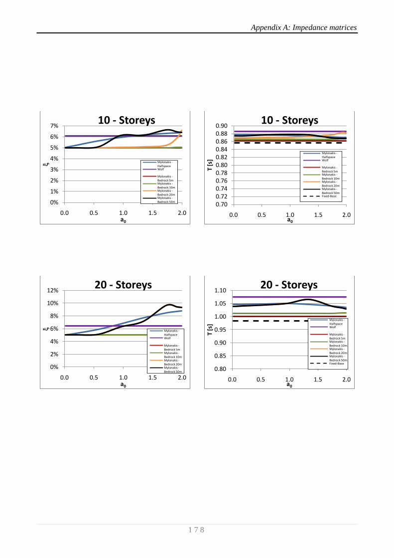
Appendix A: Impedance matrices
1 7 8
0%
1%
2%
3%
4%
5%
6%
7%
0.0 0.5 1.0 1.5 2.0
a0
10 - Storeys
Mylonakis -HalfspaceWolf
Mylonakis -Bedrock 5mMylonakis -Bedrock 10mMylonakis -Bedrock 20mMylonakis -Bedrock 50m
0.700.720.740.760.780.800.820.840.860.880.90
0.0 0.5 1.0 1.5 2.0T
[s]
a0
10 - Storeys
Mylonakis -HalfspaceWolf
Mylonakis -Bedrock 5mMylonakis -Bedrock 10mMylonakis -Bedrock 20mMylonakis -Bedrock 50mFixed-Base
0%
2%
4%
6%
8%
10%
12%
0.0 0.5 1.0 1.5 2.0
a0
20 - Storeys
Mylonakis -HalfspaceWolf
Mylonakis -Bedrock 5mMylonakis -Bedrock 10mMylonakis -Bedrock 20mMylonakis -Bedrock 50m
0.80
0.85
0.90
0.95
1.00
1.05
1.10
0.0 0.5 1.0 1.5 2.0
T [s
]
a0
20 - Storeys
Mylonakis -HalfspaceWolf
Mylonakis -Bedrock 5mMylonakis -Bedrock 10mMylonakis -Bedrock 20mMylonakis -Bedrock 50mFixed-Base
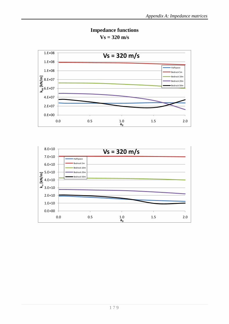
Appendix A: Impedance matrices
1 7 9
Impedance functions
Vs = 320 m/s
0.E+00
2.E+07
4.E+07
6.E+07
8.E+07
1.E+08
1.E+08
1.E+08
0.0 0.5 1.0 1.5 2.0
k hh
[kN
/m]
a0
Vs = 320 m/s
Halfspace
Bedrock 5m
Bedrock 10m
Bedrock 20m
Bedrock 50m
0.E+00
1.E+10
2.E+10
3.E+10
4.E+10
5.E+10
6.E+10
7.E+10
8.E+10
0.0 0.5 1.0 1.5 2.0
k rr[k
N/m
]
a0
Vs = 320 m/sHalfspace
Bedrock 5m
Bedrock 10m
Bedrock 20m
Bedrock 50m
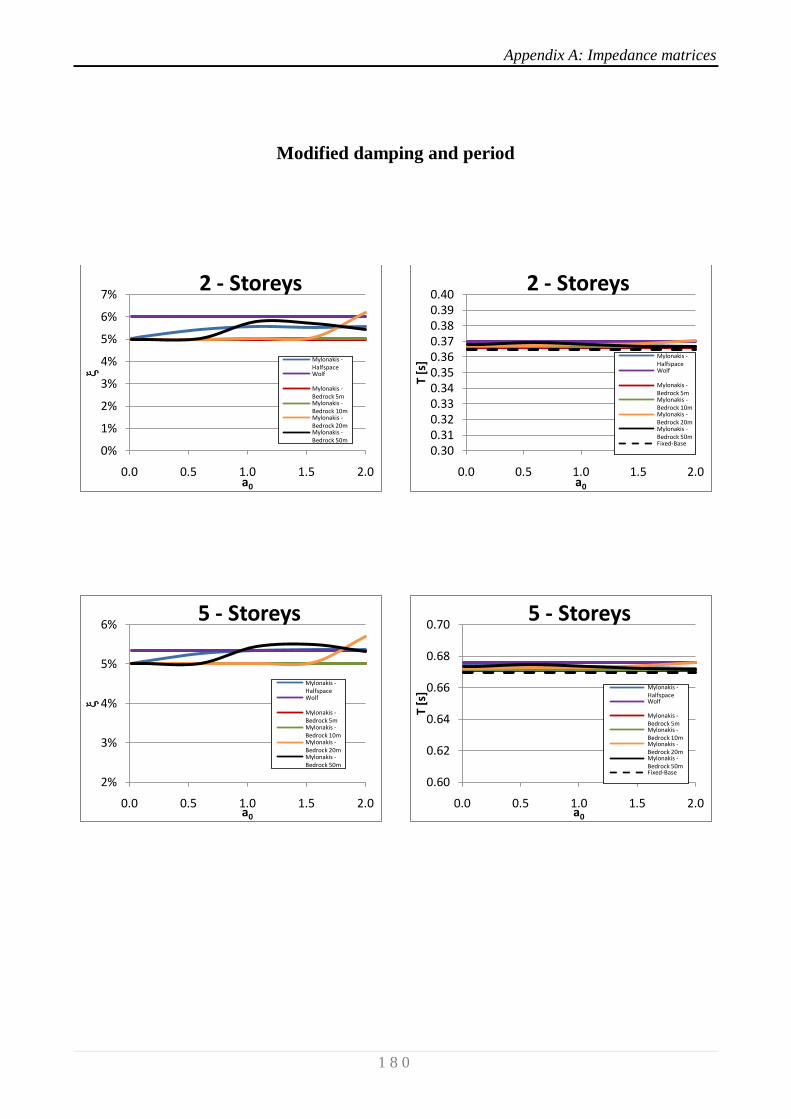
Appendix A: Impedance matrices
1 8 0
Modified damping and period
0%
1%
2%
3%
4%
5%
6%
7%
0.0 0.5 1.0 1.5 2.0
a0
2 - Storeys
Mylonakis -HalfspaceWolf
Mylonakis -Bedrock 5mMylonakis -Bedrock 10mMylonakis -Bedrock 20mMylonakis -Bedrock 50m
0.300.310.320.330.340.350.360.370.380.390.40
0.0 0.5 1.0 1.5 2.0
T [s
]
a0
2 - Storeys
Mylonakis -HalfspaceWolf
Mylonakis -Bedrock 5mMylonakis -Bedrock 10mMylonakis -Bedrock 20mMylonakis -Bedrock 50mFixed-Base
2%
3%
4%
5%
6%
0.0 0.5 1.0 1.5 2.0
a0
5 - Storeys
Mylonakis -HalfspaceWolf
Mylonakis -Bedrock 5mMylonakis -Bedrock 10mMylonakis -Bedrock 20mMylonakis -Bedrock 50m
0.60
0.62
0.64
0.66
0.68
0.70
0.0 0.5 1.0 1.5 2.0
T [s
]
a0
5 - Storeys
Mylonakis -HalfspaceWolf
Mylonakis -Bedrock 5mMylonakis -Bedrock 10mMylonakis -Bedrock 20mMylonakis -Bedrock 50mFixed-Base
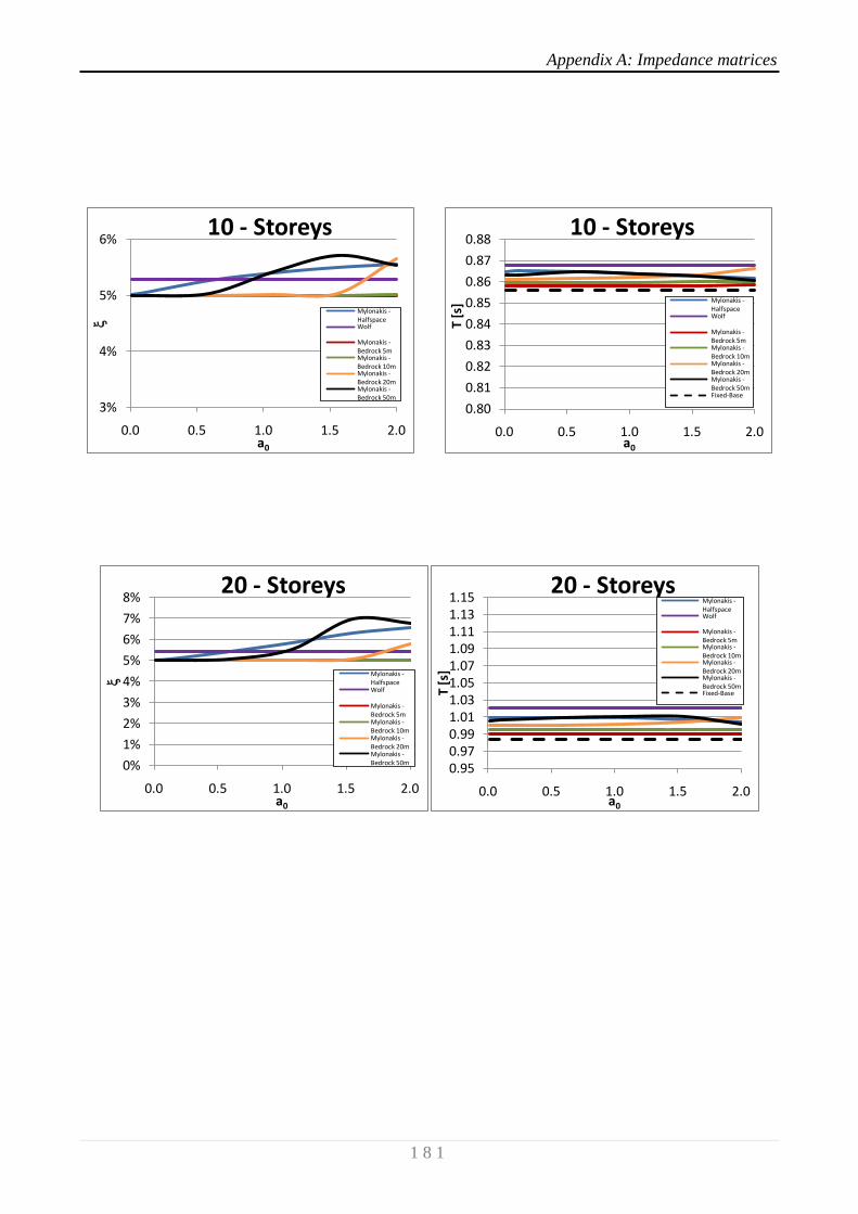
Appendix A: Impedance matrices
1 8 1
3%
4%
5%
6%
0.0 0.5 1.0 1.5 2.0
a0
10 - Storeys
Mylonakis -HalfspaceWolf
Mylonakis -Bedrock 5mMylonakis -Bedrock 10mMylonakis -Bedrock 20mMylonakis -Bedrock 50m
0.80
0.81
0.82
0.83
0.84
0.85
0.86
0.87
0.88
0.0 0.5 1.0 1.5 2.0
T [s
]a0
10 - Storeys
Mylonakis -HalfspaceWolf
Mylonakis -Bedrock 5mMylonakis -Bedrock 10mMylonakis -Bedrock 20mMylonakis -Bedrock 50mFixed-Base
0%
1%
2%
3%
4%
5%
6%
7%
8%
0.0 0.5 1.0 1.5 2.0
a0
20 - Storeys
Mylonakis -HalfspaceWolf
Mylonakis -Bedrock 5mMylonakis -Bedrock 10mMylonakis -Bedrock 20mMylonakis -Bedrock 50m
0.950.970.991.011.031.051.071.091.111.131.15
0.0 0.5 1.0 1.5 2.0
T [
s]
a0
20 - StoreysMylonakis -HalfspaceWolf
Mylonakis -Bedrock 5mMylonakis -Bedrock 10mMylonakis -Bedrock 20mMylonakis -Bedrock 50mFixed-Base

Appendix B Selected Earthquakes
1 8 2
Appendix B
Selected Earthquakes

Appendix B Selected Earthquakes
1 8 3
Location Date Mechanism
Closest
Distance
(km)
MW
Depth
of top
(km)
Depth
of
bottom
(km)
Rupture
Velocity
(km/s)
Peak
Acceleration
SN SP Vert
(cm/s2)
Peak
Velocity
SN SP Vert
(cm/s)
Peak Displacement
SN SP Vert
(cm)
1 Parkfield, CA, USA
(CO2) 27/06/1966 SS 0.1 6.2 0 3 2.2 466.8 - 250.1 75.1 - 13.7 22.5 - 3.8
2
San Fernando, CA,
USA
(PCD)
09/02/1971 RV 3.0 6.7 2.0 1266.0 780.4 696.0 120.0 42.2 57.7 31.1 22.7 18.9
3 Coyote Lake, CA,
USA (GA6) 08/06/1979 SS 1.2 5.6 2 11.85 2.8 435.6 278.9 146.9 47.5 23.9 16.5 9.3 2.9 3.1
4
Imperial Valley, CA,
USA (E07)
15/10/1979 SS 1.8 6.5 0 10.5 2.6 453.1 327.6 533.8 109.0 43.5 26.4 45.8 23.8 9.3
5
Morgan Hill, CA,
USA
(CLD)
24/04/1984 SS 0.1 6.2 0.5 12 - 803.9 979.8 376.3 61.2 69.0 15.4 8.2 13.5 2.7
6 Nahanni, Canada
(SITE1) 23/12/1985 RV 9.4 6.7 2 11 2.75 954.6 1219.0 2322.0 43.3 35.9 42.9 18.3 4.8 12.3
7 Palm Spring,CA, USA
(NPS) 08/07/1986 OB 4.0 6.1 4 15 3.0 656.9 604.0 426.5 73.6 29.3 12.1 11.9 3.5 1.2
8
Whittier Narrows, CA,
USA
(DOW)
10/10/1987 RV 16.4 6.0 12.1 17.1 2.5 207.1 125.2 149.1 30.7 7.7 3.0 3.9 1.1 0.3
9
Superstition Hills, CA,
USA
(ELC)
24/11/1987 SS 13.6 6.4 0.5 12 2.4 292.7 218.3 125.2 52.0 35.3 8.4 22.1 9.7 4.9
10 Erzincan, Turkey
(ERZ) 13/03/1992 SS 2.0 6.6 3 12 3.0 475.3 419.2 243.0 95.2 44.7 18.3 30.4 18.3 7.9
Mechanism: SS = Strike-Slip, RV = Reverse, OB = Oblique.
Component: SN = Strike Normal, SP = Strike Parallel, Vert = Vertical

1 8 4
1 8 5
References
1. Urban M. Earthquake Risk Assessment of Historiacl Structures. s.l. : PhD thesis, Doctoral
Course on Risk Management on Build Environment, Firenze And Braunschweig, 2006.
2. Pliefke T., Sperbeck S.T., Urban M., Peil U., Budelmann H. A Standardized
Methodology for Managing Disaster Risk - An Attempt to Remove Ambiguity. s.l. : 5th International
Probabilistic Workshop, Ghent, 2007.
3. Bolt B.A. Earthquakes, 2006 Centennial update - The 1906 Big One. s.l. : Freeman, 2006.
4. Augusti G., Borri C., Niemann H.J. Is aoelian risk as significant as other environmental
risks? s.l. : Reliability Engineering and System Safeti (74), 2001. pp. 227-237.
5. Romero M.P., Seed H.B. Analytical modelling of dynamic soil response in the Mexico
earthquake of September 19, 1985. s.l. : In the Mexico earthquakes 1985-Factors involved and
lessons learned. ASCE, 1986. pp.148-162.
6. Rosenblueth E. Earthquake of 28th July, 1957 in Mexico City. s.l. : Proceedings World
Conference Earthquake Engineering, Japan (1), 1960. pp. 359-379.
7. Seed H.B., Whitman R.V., Dezfulian H., Dobry R., Idriss I.M. Soil conditions and
building damage in the 1967 Caracas earthquake. s.l. : Journal of Soil Mechanics and Foundation
Division 90 (SM8), 1972. pp. 787-806.
8. Gazetas G. Analysis of machine foundation vibrations: state of the art. s.l. : International
Journal of Soil Dynamics and Earthquake Engineering (2), 1983. pp. 2-42.
9. Veletsos A. S & Meek J.W. Dynamic Behaviour of Biulding-Foundation Systems. s.l. :
Earthquake Engineering and Structural Dynamics Vol. 3, 1974. pp. 121-138.
10. Beltrami C., Lai C.G., Pecker A. Seismic Soil-Structure Interaction in Large-Diameter
Shaft Foundations. s.l. : European School for Advanced Studies in Reduction of Seismic Risk,
November 2006. Research Report No. ROSE-2006/04.
11. Lysmer J., Ukada T., Tsai C.F., Seed H.B. "FLUSH" - A Computer Program for
Approximate 3-D Analysis of Soil-Structure Interaction". s.l. : REPORT No. EERC75-30,
Earthquake Engineering Research Center, Uniersity of California, Berkeley, 1975.
12. Mylonakis G., Nikolau A., Gazetas G. Soil-Pile-Bridge seismic interaction: kinematic
and inertial effects. Part 1: soft soil. s.l. : Earthquake Engineering and Structural Dynamics Vol. 26,
1997. pp. 337-359.
13. Mylonakis G., Nikolau S., Gazetas G. Footing under seismic loading: Analysis and
design issues with emphasis on bridge foundations. s.l. : Soil Dynamics and Earthquake
Engineering 26, 2006. pp. 824-853.
14. Kramer S. Geotechnical Earthquake Engineering. s.l. : Englewood Cliffs, NJ: Prentice-
Hall, 1996.
15. Finn W.D.L. State-of-the-art of geotechnical earthquake engineerign practice. s.l. : Soil
Dynamics and Earthquake Engineering - Vol. 20 (1-4), 2000. pp. 1-15.
16. Stewart J.P., Seed R.B., Fenves G.L. Seismic Soil-Structure Interaction in buildings. II:
empirical findings. s.l. : Journal of Geotechnical Engineering ASCE 125(1), 1999. pp. 38-48.
1 8 6
17. Kim S., Stewart J.P. Kinematic Soil-Structure Interaction from strong motion
recordings. s.l. : Journal of Geotechnical and Geoenvironmental Engineering ASCE 129(4), 2003.
pp. 323-335.
18. Schnabel P.B., Lysmer J., Seed H.B. SHAKE: a computer program for earthquake
response analysis of horizontally layered sites. s.l. : Report EERC 72-12, University of California,
Berkeley, 1972.
19. Kausel E., Roesset J.M., Christian J.T. Nonlinear benaviour in Soil-Structure
Interaction. s.l. : Journal of Geotechnical Engineering Division ASCE 102(GT12). pp. 1159-1178.
20. Luco J.E. Impedance functions of a rigid foundation on a leyered medium. s.l. : Nucl Eng
Des (31), 1974. pp.204-217.
21. Kausel E., Roesset J.M. Dynamic stiffness of circular foundations. s.l. : Journal of
Engineerign Mechanics Division ASCE (101), 1975. pp.771-785.
22. Wong H.L., Luco J.E. Tables of impedance functions for square foundations on layered
media. s.l. : Soil dynamics and earthquake engineering (4), 1985. pp.64-81.
23. Dobry R., Gazetas G., Stokoe K.H. Dynamic response of arbitrarly shaped foundations:
experimental verification. s.l. : Journal of Geotechnical Engineering Division ASCE (112), 1986.
pp. 136-149.
24. Guzina B.B., Pak R.Y.S. Vertical vibration of a circular footing on a linear-wave
velocity half-space. s.l. : Geotechnique 48(2), 1998. 159-168.
25. Vrettos C. Vertical and rocking impedances for rigid rectangular foundations on soils
with bounded non-homogeneity. s.l. : Earthquake Engineering Structural Dynamics (28), 1999. pp.
1525-1540.
26. Karabalis D.L., Beskos D.E. Dynamic response of 3-D rigid surface foundations by time
domain boundary element method. s.l. : Earthquake Engineering and Structural Dynamics (12),
1984. pp. 73-93.
27. Qian, Beskos D.E. Dynamic interaction between three-dimensional rigid surface
foundations and comparison with the ATC-3 provisions. s.l. : Earthquake Engineering and
Structural Dynamics 24(3), 1995. pp. 419-437.
28. Maravas G., Mylonakis G., Karabalis D.L. Dynamic characteristics of simple
structures on piles and footings. s.l. : 4th International Conference on Earthquake Geotechnical
Engineering, 2007. Paper No. 1672.
29. Veletsos A.S., Nair V.V. Seismic interaction of structures on hysteretic foundations. s.l. :
Journal of Structural Engineering, ASCE, 101(1), 1975. pp. 109-129.
30. Veletsos A.S. Dynamics of Structure-Foundation Systems. s.l. : in: Hall, W.J. (ed.),
Structural & Geotechnical Mechanics, 1977. Prentice-Hall.
31. Mylonakis G., Gazetas G. Seismic Soil-Structure Interaction: Beneficial or Detrimental?
s.l. : Journal of Earthquake Engineering, Vol. 4 (3), 2000. pp. 277-301.
32. Ciampoli M., Pinto P.E. Effects of Soil-Structure Interaction on inelastic seismic
response of bridge piers. s.l. : Journal of Structural Engineering, ASCE 121(5), 1995. pp. 806-814.
33. Somerville P.G., Smith R.W., Graves R.W., Abrahamson N.A. Modification of
empirical strong ground motion attenuation relations to include the amplitude and duration effects
of rupture directivity. s.l. : Seismological Research Letters 68, 1997. pp. 199-222.
34. Resendiz D., Roesset J.M. Soil-Structure Interaction in Mexico City during the 1985
earthquake. s.l. : The Mexico Earthquakes - 1985 ASCE eds. Cassaro & Romero E.M., 1987. pp.
193-203.

1 8 7
35. Miranda E., Bertero V. Evaluation of strenght reduction factors of earthquake-resistant
design. s.l. : Earthquake Spectra 10(2), 1994. pp.357-379.
36. Pristley M.J.N., Park R. Strenght and ductility of concrete bridges columns under
seismic loading. s.l. : ACI Structural Journal 84(1), 1987. pp. 61-76.
37. MacRae G.A., Unocic F., Kramer S. Foundationemand Effects on Structural Ductility
D. s.l. : 7th National Conference on Earthquake Engineering, 2002. Boston, July 21-25.
38. Lysmer J., Ostadan F. & Chin C. SASSI2000 Theoretical manual - Revision 1. s.l. :
Geotechnical Engineering Division, Civil Engineering Department - University of California,
Berkeley, 1999.
39. Chin, C-C. Substructure subtraction method and dynamic analysis of pile foundations.
s.l. : Ph.D. Dissertation, University of California, Berkeley, 1998.
40. Lysmer, J. Analytical procedures in soil dynamics. s.l. : Report N. EERC 78/29,
Berkeley, 1978.
41. Seed H.B. & Idriss I.M. The influence of soil conditions on ground motion during
earthquake. s.l. : Journal of Soil Mechanics and Foundations, Div. ASCE, 94:99-137, 1969.
42. Waas, G. Earth vibration effects and abatement for military facilities - Analysis method
for footing vibrations through layered media. s.l. : Technical Report 5-71-14 US Army Engineer
Waterways Experimental Station, Vicksburg, Mississipi, 1972.
43. Lysmer J. & Waas G. Shear waves in palne infinite structures. s.l. : Journal of
Engineering Mechanics, Div. ASCE 98:85-105, 1972.
44. Kausel E. & Tassoulas J.L. Transmitting boundaries: a closed form comparison. s.l. :
Bulletin of the Seismological Society of America, 71:143-159, 1981.
45. Chen J-C. Analysis of local variation in free-field ground motions. s.l. : Ph.D.
Dissertation, University of California, Berkeley, 1980.
46. Lysmer J. & Kuhlemeyer. Finite dynamic model for infinite media. s.l. : Journal of
Engineering Mechanics, Div. ASCE, 95:859-877 , 1969.
47. Lysmer J., Tabatabaie-Raissi M., Tajirian F., Vahdani S. & Ostadan F. SASSI - A
System for Analysis of Soil-Structure Interaction. s.l. : Report N. UCB/GT/81-02, Geotechnical
Engineering, University of California, Berkeley, 1981.
48. Chopra A. Dynamics of structures - Theory and applications to earthquake engineering,
Third Edition. s.l. : Prentice Hall, 2007.
49. Clough R.W. & Penzien J. Dynamics of structures. s.l. : Computers and structures, Inc.,
2003.
50. Canadian commission on building and fires code. The National Building Code of
Canada. s.l. : National Research Council, Ottawa, 2005.
51. Government of the federal district. Complementary technical norms for seismic design.
s.l. : Official Gazette of the Federal District, Mexico, 2004.
52. Bommer J.J., Acevedo A.B. The use of real earthquake accelerograms as input to
dynamic analysis. s.l. : Journal of Earthquake Engineering 8, Special Issue, 1, 2004. pp. 43–91.
53. Iervolino I., Maddaloni G., Cosenza E. Eurocode 8 Compliant Real Record Sets for
Seismic Analysis of Structures. s.l. : Journal of Earthquake Engineering, 12, 2008. pp. 54–90.
54. Iervolino I., Galasso C, Cosenza E. REXEL: computer aided record selection for code-
based seismic structural analysis. s.l. : Bulletin of Earthquake Engineering, 2009.
55. Aki K. Seismic displacement near a fault. s.l. : Journal of Geophysical Research (73), pp.
5359–5376, 1968.

1 8 8
56. Bertero V.V., Mahin S.A., Herrera R.A. Aseismic design implications of nearfault San
Fernando earthquake records. s.l. : Earthquake Engineering and Structural Dynamics (6), pp.31–
42, 1978.
57. Mavroeidis G.P., Papageorgiou A.S. A mathematical representation of Near-Fault
ground motions. s.l. : Bulletin of the Seismological Society of America, 2003. Vol. 93 (3), pp.
1099-1131.
58. Tothong, P. Probabilistic seismic demand analysis using advanced, ground-motion
intensity measures, attenuation, relationships, and near-fault effects. s.l. : Ph.D. thesis. Department
of Civil and Environmental Engineering. Stanford University, CA. Advisor: C.A. Cornell, 2007.
59. Somerville, P. G., Smith, N., Graves, R., Abrahamson, N. Modification of empirical
strong ground-motion attenuation results to include the amplitude and duration effects of rupture
directivity. s.l. : Seismology Research Letters, 68, 1997. pp. 199–222.
60. Iervolino, I., Galasso, C., Cosenza, E. Selezione assistita di input sismico e nuove Norme
Tecniche per le Costruzioni. Rome : Proc. of "Valutazione e riduzione della vulnerabilità sismica di
edifici esistenti in c.a." (in italian), 2009.
61. Ambraseys, N., Smit, P., Sigbjornsson, R., Suhadolc, P. Margaris, B. Internet-Site for
European Strong-Motion Data. s.l. : European Commission, Research-Directorate General,
Environment and Climate Programme, 2002.
62. ITACA, Working Group. Data Base of the Italian strong motion data. 2008.