Inflation Dynamics and the Great Recession dynamics.pdf337 laurence ball Johns Hopkins University...
69
337 LAURENCE BALL Johns Hopkins University SANDEEP MAZUMDER Wake Forest University Inflation Dynamics and the Great Recession ABSTRACT This paper examines inflation dynamics in the United States since 1960, with a particular focus on the Great Recession. A puzzle emerges when Phillips curves estimated over 1960–2007 are used to predict inflation over 2008–10: inflation should have fallen by more than it did. We resolve this puzzle with two modifications of the Phillips curve, both suggested by theories of costly price adjustment: we measure core inflation with the weighted median of consumer price inflation rates across industries, and we allow the slope of the Phillips curve to change with the level and variance of inflation. We then examine the hypothesis of anchored inflation expectations. We find that expectations have been fully “shock-anchored” since the 1980s, while “level anchoring” has been gradual and partial, but significant. It is not clear whether expectations are sufficiently anchored to prevent deflation over the next few years. Finally, we show that the Great Recession provides fresh evidence against the New Keynesian Phillips curve with rational expectations. I n his presidential address before the American Economic Association, Milton Friedman (1968) presented a theory of the short-run behavior of inflation in which inflation depends on expected inflation and the gap between unemployment and its natural rate. Friedman also suggested that “unanticipated inflation . . . generally means . . . a rising rate of inflation,” or in other words, that expected inflation is well proxied by past inflation. These assumptions imply an accelerationist Phillips curve that relates the change in inflation to the unemployment gap. In the decades since Friedman’s work, his model has been a workhorse of macroeconomics. Researchers have refined the model extensively; two of the numerous examples are Robert Gordon’s (1982, 1990) introduction Copyright 2011, The Brookings Institution
Transcript of Inflation Dynamics and the Great Recession dynamics.pdf337 laurence ball Johns Hopkins University...

337
laurence ballJohns Hopkins University
sandeep mazumderWake Forest University
Inflation Dynamics and the Great Recession
ABSTRACT This paper examines inflation dynamics in the United States since 1960, with a particular focus on the Great Recession. A puzzle emerges when Phillips curves estimated over 1960–2007 are used to predict inflation over 2008–10: inflation should have fallen by more than it did. We resolve this puzzle with two modifications of the Phillips curve, both suggested by theories of costly price adjustment: we measure core inflation with the weighted median of consumer price inflation rates across industries, and we allow the slope of the Phillips curve to change with the level and variance of inflation. We then examine the hypothesis of anchored inflation expectations. We find that expectations have been fully “shock-anchored” since the 1980s, while “level anchoring” has been gradual and partial, but significant. It is not clear whether expectations are sufficiently anchored to prevent deflation over the next few years. Finally, we show that the Great Recession provides fresh evidence against the New Keynesian Phillips curve with rational expectations.
In his presidential address before the American Economic Association, Milton Friedman (1968) presented a theory of the short-run behavior
of inflation in which inflation depends on expected inflation and the gap between unemployment and its natural rate. Friedman also suggested that “unanticipated inflation . . . generally means . . . a rising rate of inflation,” or in other words, that expected inflation is well proxied by past inflation. These assumptions imply an accelerationist Phillips curve that relates the change in inflation to the unemployment gap.
In the decades since Friedman’s work, his model has been a workhorse of macroeconomics. Researchers have refined the model extensively; two of the numerous examples are Robert Gordon’s (1982, 1990) introduction
Copyright 2011, The Brookings Institution

338 Brookings Papers on Economic Activity, spring 2011
of supply shocks and Douglas Staiger and others’ (1997) modeling of a time-varying natural rate of unemployment. Economists have debated how well the accelerationist Phillips curve fits the data, some declaring the equation’s demise and others reporting that “The Phillips Curve Is Alive and Well” (Fuhrer 1995).
Debate over the Phillips curve has gained momentum during the U.S. economic slump that began in 2007. Some economists see a puzzle: inflation has not fallen as much as a traditional Phillips curve would have predicted, given the high level of unemployment. For example, in September 2010 John Williams (now president of the Federal Reserve Bank of San Francisco) said, “The surprise [about inflation] is that it’s fallen so little, given the depth and duration of the recent downturn. Based on the experience of past severe recessions, I would have expected inflation to fall by twice as much as it has” (Williams 2010, p. 8).
In addition to analyzing the recent behavior of inflation, economists are debating its likely path in the future. If the accelerationist Phillips curve is accurate, then today’s high unemployment implies a substantial risk that inflation will fall below zero. Yet many economists argue that deflation is unlikely, primarily because the Federal Reserve’s commitment to a low but positive inflation rate has “anchored” inflation expectations. According to Federal Reserve Chairman Ben Bernanke, “Falling into deflation is not a sig-nificant risk for the United States at this time, but that is true in part because the public understands that the Federal Reserve will be vigilant and proactive in addressing significant further disinflation” (Bernanke 2010, p. 17).
This paper contributes to the debate over past and prospective inflation in several steps. We first show why it is easy to view the recent behavior of inflation as puzzling. We estimate accelerationist Phillips curves with quarterly data for the period 1960–2007, measuring inflation with either the consumer price index (CPI) or the CPI less food and energy (XFE), the standard measure of “core” inflation. We use the estimated equation and the path of unemployment over 2008–10 to produce dynamic forecasts of inflation. In these forecasts a 4-quarter moving average of core inflation falls to -4.3 percent in 2010Q4. In reality, 4-quarter core inflation was 0.6 percent in 2010Q4. A simple Phillips curve thus predicts a deflation that did not occur.
We show, however, that two simple modifications of the Phillips curve eliminate this puzzle. They produce a specification that fits the entire period since 1960, including the Great Recession. Both modifications are suggested by theory: specifically, by models from the 1980s and 1990s that incorporate costly adjustment of nominal prices.

laurence ball and sandeep mazumder 339
First, following Michael Bryan and Stephen Cecchetti (1994), we measure core inflation with a weighted median of price changes across industries. This approach is motivated by price adjustment models in which unusually large changes in relative prices cause movements in aggregate inflation. Median inflation fell by more than XFE inflation from 2007 to 2010, reflect-ing a higher initial level: in 2007, median inflation was about 3 percent per year and XFE inflation was 2 percent. The relatively large fall in median inflation reduces the gap between forecast and actual inflation.
Second, following Ball, Gregory Mankiw, and David Romer (1988), we allow the slope of the Phillips curve—that is, the coefficient on unemployment—to vary over time. In the Ball-Mankiw-Romer theory, the Phillips curve steepens if inflation is high or variable, or both, because these conditions reduce nominal price stickiness. U.S. time-series evidence strongly supports this prediction; in particular, the Phillips curve has been relatively flat in the low-inflation period since the mid-1980s. A flatter Phillips curve reduces the forecast fall in inflation over 2008–10. When we account for this effect and measure core inflation with the median price change, forecast 4-quarter core inflation in 2010Q4 is 0.3 percent, close to the actual level of 0.5 percent.
After presenting these results, we turn to the idea of anchored expec-tations. We distinguish between “shock anchoring,” which means that expectations do not respond to supply shocks, and “level anchoring,” which means that expectations stay fixed at a certain level regardless of any move-ments in actual inflation. We assume this level is 2.5 percent per year for core CPI inflation (which corresponds to about 2 percent for core inflation as measured by the deflator for personal consumption expenditures, or PCE). Based on the behavior of actual inflation and of expectations (as measured by the Survey of Professional Forecasters), we find that expectations have been fully shock-anchored since the 1980s. Level anchoring has been grad-ual and partial, but significant. According to our estimates, the fraction of a change in core inflation that is passed into expectations fell from roughly 1.0 in 1985 to between 0.4 and 0.7 in 2010.
Following our analysis of recent inflation, we forecast inflation over 2011–13, using our estimates of the Phillips curve through 2010 and Con-gressional Budget Office (CBO) forecasts of unemployment and output over the forecast period. Here the results depend crucially on whether we incor-porate anchored expectations into our equation. Our basic accelerationist specification explains why inflation is currently positive but also predicts that deflation is on the way. In contrast, the degree of expectation anchoring estimated for 2010 is high enough to keep inflation positive. We are not

340 Brookings Papers on Economic Activity, spring 2011
confident in this forecast, however, because it assumes that expected infla-tion will stay anchored at 2.5 percent per year for several years, at a time when actual inflation is less than 1 percent.
Most of this paper examines Phillips curves in which expected infla-tion depends on past inflation and possibly the Federal Reserve’s target. A large literature since the 1990s studies an alternative model, the “New Keynesian” Phillips curve based on rational expectations and Guillermo Calvo’s (1983) model of staggered price adjustment. The last part of this paper asks whether the New Keynesian Phillips curve helps explain the recent behavior of inflation; the answer is no. Indeed, the last few years provide fresh evidence of the poor empirical performance of the model, especially the version of Jordi Galí and Mark Gertler (1999) in which marginal cost is measured with labor’s share of income. This specification produces a counterfactual prediction of rising inflation over 2008–10.
Parts of our analysis overlap with other recent research on the Phillips curve, such as that by Jeffrey Fuhrer and others (2009), Fuhrer and Giovanni Olivei (2010), and James Stock and Mark Watson (2008, 2010). We com-pare our results with those of previous work throughout the paper. One difference from Stock and Watson’s work is that they focus on forecasting inflation in real time. In seeking to understand inflation behavior, we freely use information that is not available in real time, such as the 2011 CBO series for the natural rate of unemployment.
I. A Simple Phillips Curve and a Puzzle
We first introduce a conventional Phillips curve and then show that it predicts a large deflation over 2008–10.
I.A. The Phillips Curve
Milton Friedman’s Phillips curve can be expressed as
( ) * ,1 π π αt te
t tu u= + −( ) + e
where p is annualized quarterly inflation, pe is expected inflation, u is unemployment, u* is the natural rate of unemployment, and e is an error term that we assume is uncorrelated with u - u*. A common variant of this equation replaces u - u* with the gap between actual and potential output. Since Friedman wrote, theorists have derived equations that are broadly similar to equation 1 from models in which price setters have incomplete

laurence ball and sandeep mazumder 341
information (for example, Lucas 1973, Mankiw and Reis 2002) or in which nominal prices are sticky (for example, Roberts 1995).1
We follow a long tradition in applied work that assumes backward-looking expectations: expected inflation is determined by past inflation. Specifically, we assume that expected inflation is the average of inflation in the past 4 quarters. In this case equation 1 becomes
( ) * .21
4 1 2 3 4π π π π π αt t t t t t tu u= + + +( ) + −( ) +− − − − e
This equation is a special case of the Phillips curves estimated by Gordon and by Stock and Watson, which generally include lags of unemployment and lags of inflation with unrestricted coefficients (except for the accelerationist assumption that the coefficients sum to 1). We keep our specification par-simonious along this dimension so that we can enrich it more easily along others (for example, by allowing time variation in the coefficient a). We examine versions of equation 2 with richer lag structures as part of our robustness checks.
The structure of inflation lags in equation 2 implies that a 1-percentage-point increase in unemployment for 1 quarter changes inflation in the long run by 0.4 times the coefficient a. The long-run effect of a 1-percentage-point increase in unemployment sustained for a year is 1.6 times a.2
Our empirical work requires a series for either the natural rate of unemployment or potential output. For most of our analysis, we use estimates of these variables from the CBO; as a robustness check, we also estimate a path for the natural rate using a technique from Staiger and others (1997).
1. The assumption that u - u* is uncorrelated with the error in the Phillips curve, implying that ordinary least squares estimates of the equation are unbiased, is standard in the literature but rarely examined. We interpret the error term as summarizing the effects of relative price changes, which influence inflation when some nominal prices are sticky (see section II). We assume that these relative-price effects are uncorrelated with the aggregate variable u - u*. We maintain this assumption when p is a measure of core inflation, which strips away any effects of relative price changes but does so imperfectly. In this case the error summarizes the relative-price effects that are not removed from core inflation. This approach to identifi-cation ignores the problem of measurement error. The variable u is an imperfect measure of the activity variable in the Phillips curve, and u* is an imperfect measure of the natural rate of unemployment. These problems bias our estimates of the coefficient a toward zero. Future work should investigate the size of this bias and more generally the identification problem for the Phillips curve.
2. The easiest way to derive this result is to numerically calculate the path of inflation following an increase in unemployment.

342 Brookings Papers on Economic Activity, spring 2011
The CBO’s natural rate series is similar to estimates from other sources: the natural rate rises modestly in the 1960s and 1970s, from about 5.5 percent to 6.3 percent, then falls to 5.0 percent in the 1990s. It remains at 5.0 percent through 2007 and then rises slightly to 5.2 percent in 2009.
Since Gordon (1982), many empirical researchers add supply shocks to the Phillips curve. Others seek to filter supply shocks out of the dependent variable with measures of core inflation. The most common supply shocks are changes in the relative prices of food and energy, and the standard core inflation measure is inflation less food and energy. Most of this paper examines core inflation, but we experiment with alternative measures of this variable.
I.B. The Puzzle
We now take our first pass at estimating the Phillips curve. We want to know whether equation 2 fits the behavior of inflation since 1960, and especially whether anything changed during the Great Recession. The starting date of 1960 is based on Robert Barsky (1987), who finds a regime change in the univariate behavior of inflation at that point, from a station-ary process to an IMA(1,1) process (an IMA, or integrated moving average, process is one that still captures inflation behavior, albeit with time-varying parameters, according to Stock and Watson 2010).
We estimate equation 2 for the period 1960–2007, thus ending the sample at the start of the Great Recession. We examine two measures of inflation, one derived from the CPI (total or “headline” inflation) and one from the CPI excluding food and energy (XFE inflation). In each case we average monthly data on the price level to create quarterly price levels and then compute annualized percentage changes from quarter to quarter. For each inflation variable we estimate a Phillips curve that includes the unemployment gap and one that includes the output gap.
Table 1 presents our regression results. For both measures of inflation, the coefficients on the unemployment gap are about -0.5 and are highly significant statistically (t > 5). The coefficients on the output gap are around 0.25, which accords with the unemployment gap coefficients and Okun’s Law.
Recall that 1 percentage-point-year of increased unemployment or output changes long-run inflation by 1.6 times the variable’s coefficient. For example, in the equation with XFE inflation and output, the estimated coefficient implies an effect of approximately (1.6)(0.25) = 0.4 percentage
point. Equivalently, the sacrifice ratio for reducing inflation is 1
0 42 5
.. .=
laurence ball and sandeep mazumder 343
This result is in the ballpark of previous estimates of U.S. sacrifice ratios (for example, Ball 1994).
Next we perform dynamic forecasts of inflation over 2008–10. We start with actual inflation through 2007 and feed the path of unemployment over 2008–10 into the estimated Phillips curves in table 1. Figure 1 compares the forecast and actual levels of total inflation (top panel) and XFE inflation (bottom panel). We present 4-quarter moving averages so that we can ignore some of the transitory fluctuations in the quarterly data.
Figure 1 illustrates why some economists think the Phillips curve has broken down recently. Actual XFE inflation, for example, fell from 2.3 per-cent in 2007Q4 to 0.6 percent in 2010Q4. In the dynamic forecasts, how-ever, XFE inflation falls to -4.3 percent for the unemployment equation and -3.3 percent for the output equation. The pre-2008 Phillips curve thus predicts a deflation that did not occur.
II. Measuring Core Inflation
Here we compare alternative measures of core inflation. We start by discuss-ing supply shocks, the fluctuations in inflation that core measures are meant to filter out.
II.A. Measuring Supply Shocks
The Phillips curve used in much applied work is Gordon’s (1990) “triangle model.” It explains total inflation with three factors: expected inflation,
Table 1. regressions estimating the Traditional phillips curve slope over 1960Q1–2007Q4a
Estimatesusingthe unemploymentgap Estimatesusingtheoutputgapb
Measuring Measuring Measuring MeasuringIndependent inflationas inflationas inflationas inflationasvariable totalinflation XFEinflation totalinflation XFEinflation
Unemployment -0.507 -0.474 0.308 0.257 or output gap (0.091) (0.077) (0.049) (0.042)Adjusted R2 0.703 0.746 0.713 0.744
Source: Authors’ regressions.a. Equation 2 in the text is estimated by the ordinary least squares method; standard errors are in
parentheses.b. The output gap (y - y*)t (the logarithm of real GDP minus the logarithm of the Congressional Budget
Office’s estimate of potential real GDP) is substituted for the unemployment gap (u - u*)t in equation 2.

344 Brookings Papers on Economic Activity, spring 2011
Figure 1. dynamic Forecasts of consumer price Inflation, 2008–10a
Total inflation
5
4
3
2
1
0
–1
–2
Actual
Forecast from output gap
Forecast from unemployment gap
2000 2001 2002 2003 2004 2005 2006 2007 2008 2009 2010
Source: Authors’ calculations. a. Actual data and forecasts are 4-quarter moving averages. Forecasts are derived from the regression
results in table 1 using data for the period 1960Q1–2007Q4.
Percent per year
XFE inflation
3
2
1
0
–1
–2
–3
–4
Actual
Forecast from output gap
Forecast from unemployment gap
2000 2001 2002 2003 2004 2005 2006 2007 2008 2009 2010
Percent per year

laurence ball and sandeep mazumder 345
aggregate activity, and supply shocks. The most common measures of supply shocks are changes in the relative prices of food and energy. Since the 1970s these variables have added greatly to the adjusted R2s of estimated Phillips curves.
Theoretically, however, it is not obvious why only certain relative prices should influence inflation—why it depends on food and energy prices rather than, say, the prices of clothing and home appliances. As Friedman asked, “Why should the level of all prices be affected significantly by changes in the prices of some things relative to others?”3 A number of economists answer this question with models of nominal price stickiness. Many, ranging from Rudiger Dornbusch and Stanley Fischer’s (1990) textbook to Olivier Blanchard and Galí (2008), assume that food and energy prices are flexible whereas other prices are sticky. In this setting, a shock that raises the relative prices of food and energy does so by increasing their nominal prices while other prices stay constant. This pattern of adjustment implies an increase in the aggregate price level.
Ball and Mankiw (1995) present a theory of supply shocks based on a different sticky-price model. Rather than assume that certain industries have sticky or flexible prices, Ball and Mankiw make price adjustment endogenous. Firms experience shocks to their equilibrium relative prices and choose whether to pay a menu cost and adjust prices. In each period the firms that receive the largest shocks are the most likely to adjust. The upshot is that inflation depends on the distribution of price changes across industries. If the distribution is skewed to the right, for example, that means that many firms have desired price increases that are large enough to trig-ger adjustment, and relatively few have large enough negative shocks to adjust. As a result, the aggregate price level rises. Based on this result, Ball and Mankiw measure supply shocks with the skewness of relative price changes and other measures of asymmetry.
In practice, the competing measures of supply shocks—food and energy prices and asymmetries in price distributions—are positively correlated. The reason is that, in many periods, large changes in food and energy prices create large tails in price distributions. Yet there is enough independent variation in supply-shock measures to indicate which are most closely related to inflation. For the period 1949–89, Ball and Mankiw show that only price-change asymmetries, not changes in food and energy prices, are significant when both are included in a Phillips curve.
3. Milton Friedman, “Perspective on Inflation,” Newsweek, June 24, 1975, p. 73.

346 Brookings Papers on Economic Activity, spring 2011
II.B. From Supply Shocks to Core Inflation
We define core inflation as the part of inflation explained not by sup-ply shocks, but rather by expected inflation and economic activity—the two other parts of the triangle. With this definition one can measure core inflation by removing the effects of supply shocks from total inflation. This approach follows common practice. When researchers measure supply shocks with changes in food and energy prices, they measure core inflation with XFE inflation, which strips away the direct effects of food and energy.
If supply shocks are asymmetries in the distribution of price changes, then a measure of core inflation should eliminate the effects of these asymme-tries. A simple measure, proposed by Bryan and Cecchetti (1994), is the weighted median of price changes across industries (median inflation).
Researchers sometimes evaluate core inflation measures by their ability to forecast future inflation. In theory, core inflation as we define it might not be a good forecaster. A rise in total inflation caused by a supply shock might raise expected inflation, which in turn raises future inflation; in that case, total inflation would be a better forecaster than core inflation. In practice, however, papers such as those by Martin Sommer (2004) and Mark Hooker (2002) find that, since the 1980s, supply shocks have not fed strongly into future inflation; thus, core inflation is a good forecaster. We return to this point when we discuss the anchoring of inflation expectations.
Julie Smith (2004) compares median inflation and XFE inflation as fore-casters of total inflation over 1982–2000. She finds that forecasts based on median inflation are more accurate.
II.C. Measuring Median Inflation
The Federal Reserve Bank of Cleveland maintains a monthly series for median inflation that begins in 1968. The economy is disaggregated into about 40 industries (the number rises from 36 to 45 over time), and core inflation is measured by the weighted median of industry inflation rates, using the industries’ weights in the CPI.
The data include an “original” weighted median for 1967–2007 and a “revised” median for 1983 to the present. The main difference is that the original data include owners’ equivalent rent (OER) as the price for one large industry, whereas the revised data include OER for each of four geographic regions. This revision makes some difference because the change in OER (in the original data) or one of the regional changes (in the revised data) is the median price change for around half of the observations. For the period

laurence ball and sandeep mazumder 347
when the two median series overlap, the differences are modest, although the original series shows somewhat greater monthly volatility.4
We compute quarterly data for median inflation that match the timing of our quarterly series for total and XFE inflation. We first use the monthly median inflation rates from the Cleveland Fed to construct a monthly series for price levels. Then we average 3 months to get quarterly price levels and compute annualized percentage changes in that variable.5
The aggregation of median inflation over time is not straightforward. As an alternative to our approach, one could measure the median of quarterly price changes across industries; in principle, this median might differ greatly from the quarterly variable that we construct from monthly medians. This nonrobustness arises because the median is not a linear function of industry price changes. Future research might compare measures of median inflation based on different frequencies for industry-level data.
II.D. Some New Evidence
We present one new piece of evidence on the measurement of core inflation. Both expected inflation and the activity gap are persistent series, and hence the part of inflation they determine—core inflation—is also per-sistent. One should not expect significant transitory movements in quarterly core inflation. Therefore, one criterion for judging core inflation measures is the extent to which their movements are permanent or transitory.
We implement this idea with Stock and Watson’s (2007) procedure for decomposing inflation into permanent and transitory components. Stock and Watson assume that inflation is the sum of a permanent, random walk component and a transitory, white noise component. This specification
4. For more documentation of the Cleveland Fed data, see Bryan and Pike (1991) and Bryan and others (1997). Some economists (including one of our discussants) question the use of median CPI as an inflation measure because the median price change in the Cleveland Fed data is often the change in one of the regional OERs. It is not clear to us why the validity of the Cleveland Fed’s approach should depend on which industry is the median. Nonetheless, as a robustness check, we have constructed median nonhousing inflation by discarding the regional OERs and computing the median price change for all other industries. A 4-quarter average of this series falls by 2.1 percentage points between 2007Q4 and 2010Q4 (from 3.1 percent to 1.0 percent); the fall in the Cleveland Fed’s median, 2.6 percentage points, is somewhat larger. Yet housing prices have a greater effect on the other leading measure of core inflation, XFE. This variable falls by 1.7 percentage points between 2007Q4 and 2010Q4; if the OERs are removed along with food and energy, the resulting inflation measure falls by only 0.9 percentage point.
5. The Cleveland Fed website provides a different measure of quarterly inflation: the average of median inflation over the 3 months of the quarter.

348 Brookings Papers on Economic Activity, spring 2011
implies that aggregate inflation follows an IMA(1,1) process. Stock and Watson allow the variances of the permanent and transitory shocks to change over time. They estimate series for the permanent component of inflation and the variances of the two shocks.
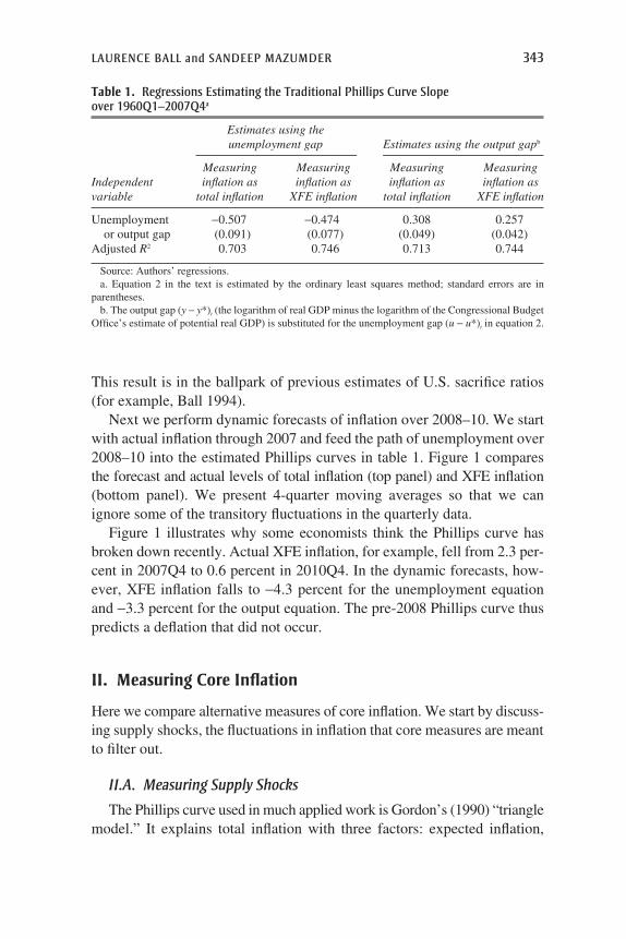
We apply the Stock-Watson procedure to the two competing measures of core inflation, XFE inflation and median inflation. Figure 2 shows the quarterly series for these two variables and their estimated permanent components. The sample starts in 1983Q2, when the Cleveland Fed’s “revised” median data begin. The divergences between total and per-manent inflation—the transitory shocks—are smaller when inflation is measured by median inflation. This difference is especially pronounced in the 2000s, when median inflation appears to have almost no transitory component. These results bolster the case for measuring core inflation with the median.
The two core inflation measures behave differently because price changes that are large relative to aggregate inflation—annualized monthly changes of 20 percent or more—occur frequently in other industries besides food and energy alone. Some of these industries, such as used cars and lodging away from home, may be affected indirectly by energy prices, but others, such as women’s apparel, are not. Large price changes in all these industries cause transitory movements in XFE inflation, but their effects are filtered out by the Cleveland Fed median.
II.E. Median Inflation during the Great Recession
An important fact for our purposes is that median inflation has fallen somewhat more than XFE inflation during the Great Recession and its aftermath. Over the period from 2007Q4 to 2010Q4, the 4-quarter mov-ing average of median inflation fell from 3.1 percent to 0.5 percent, while the 4-quarter moving average of XFE inflation fell from 2.3 percent to 0.6 percent. Median inflation fell by more primarily because it started at a higher level: it was relatively high in 2007 because the distribution of price changes was skewed to the left during many months of the year. This skewness resulted from large price decreases in various industries. In March 2007, for example, the prices of jewelry and watches fell at an annu-alized rate of 30 percent, prices of car and truck rentals fell 22 percent, and prices for lodging away from home fell 13 percent. These price decreases reduced XFE inflation but not median inflation.
The relatively large fall in the median goes in the right direction for reducing the divergence between actual and forecast inflation over 2008–10. Yet changing the definition of core inflation is far from enough to resolve
laurence ball and sandeep mazumder 349
Figure 2. median and XFe consumer price Inflation and Their permanent components, 1983Q2–2010Q4
Median inflationa
4
3
2
1
0
Total
Permanent componentb
1984 1986 1988 1990 1992 1994 1996 1998 2000 2002 2004 2006 2008
Source: Authors’ calculations. a. Monthly median price levels are constructed from monthly median inflation rates from the Federal
Reserve Bank of Cleveland (each monthly rate is the rate for the median industry, where industries are weighted by their share in the CPI) and then converted to quarterly price levels by taking 3-month averages; median inflation rates are then calculated as the annualized percentage changes in these quarterly price levels.
b. Calculated using Stock and Watson’s (2007) procedure for decomposing inflation into permanent and transitory components.
Percent per year
XFE inflation
4
3
2
1
0
Total
Permanent component
1984 1986 1988 1990 1992 1994 1996 1998 2000 2002 2004 2006 2008
Percent per year
5
2010
2010

350 Brookings Papers on Economic Activity, spring 2011
the puzzle in figure 1. We also need another modification of the Phillips curve, which we turn to next.
III. A Phillips Curve with a Time-Varying Slope
As we have discussed, models of costly price adjustment provide a ratio-nale for measuring core inflation with median inflation. These models also imply time variation in the slope of the Phillips curve. As shown by Ball, Mankiw, and Romer (1988), if nominal price adjustment is costly, firms will choose to adjust more frequently when the level of inflation is higher and when the variance of inflation is higher. More frequent nominal adjust-ment makes the aggregate price level more flexible, steepening the Phillips curve. That is, the unemployment coefficient a increases in absolute value with the level and variance of inflation.
Ball, Mankiw, and Romer present international evidence supporting their model. In a cross-country regression using data from 43 countries, the average level of inflation has a strong effect on the Phillips curve slope. Robert DeFina (1991) finds a similar effect in U.S. time-series data.
Here we document time variation in the slope of the Phillips curve from 1960 through 2010. We then show that this variation is tied closely to the level and variance of inflation, as predicted by theory. Finally, we explore the implications for inflation during the Great Recession and in the future.
III.A. Estimates of a Time-Varying Slope
We generalize the basic Phillips curve, equation 2, as follows:
( ) *31
4 1 2 3 4π π π π π α
α
t t t t t t t tu u= + + +( ) + −( ) +− − − − e
tt t t= +−α η1 ,
where e and h are white noise errors with variances V and W, respectively. This specification allows the coefficient a to vary over time; specifically, it follows a random walk.
Equation 3 is a standard regression equation with a time-varying coefficient. We estimate two versions of this specification. In the first, we assume a value for the ratio of the two shock variances, V and W. With this restriction, we can estimate the path of at with the Kalman smoother. We choose V/W to create a degree of smoothness in at that appears plausible. Our intuition is that firms’ price-setting policies, which determine the Phillips
laurence ball and sandeep mazumder 351
curve slope, do not vary greatly from quarter to quarter. Emmanuel De Veirman (2009) uses a similar approach to estimate a time-varying Phillips curve slope for Japan.
In the second version of our procedure, we estimate the shock variances V and W along with the path of at. As suggested by Andrew Harvey (1989, chapter 3) and Jonathan Wright (2010), we choose the two variances to maximize the likelihood produced by the Kalman smoother. This method is roughly equivalent to choosing the variances to minimize one-step-ahead forecast errors from the model.6
We estimate equation 3 for the period 1960–2010. For observations over 1984Q2–2010Q4, we measure inflation with the Cleveland Fed’s revised median. For 1968Q2–1984Q1, we use the original median. For 1960Q1–1968Q1, when the median is not available, we use XFE inflation. We obtain similar results (not shown) when we use XFE inflation for the entire sample; the measurement of core inflation is not critical for our results regarding the Phillips curve slope.
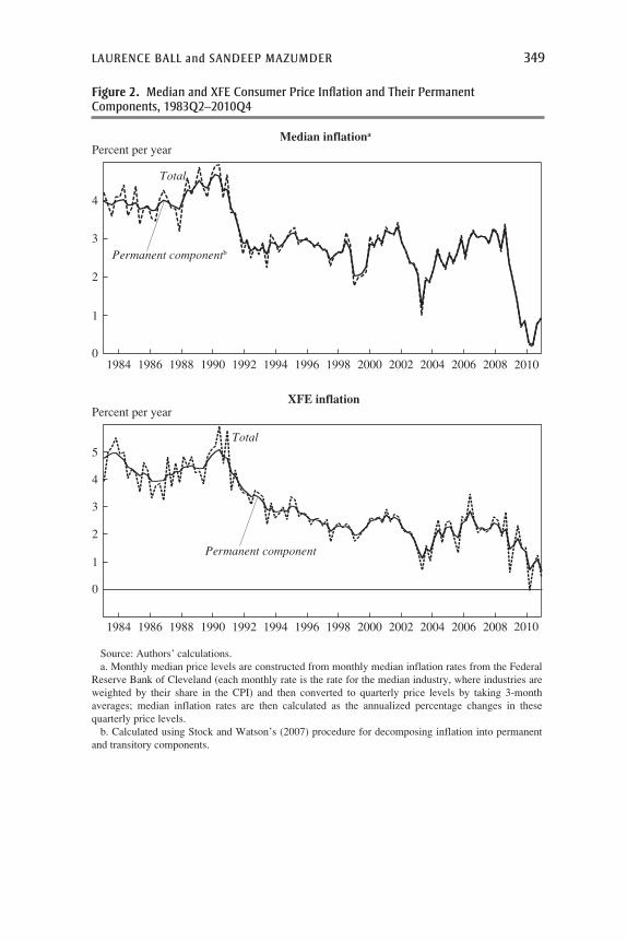
Figure 3 presents estimates of the path of at, along with 2-standard-error bands. The top panel shows the results when the two shock variances are estimated freely, and the bottom panel imposes the restriction that V/W, the ratio of the variances of e and h, is 100. (Higher values of V/W produce smoother series for a, and lower values produce more variable series.)
The two panels show the same broad trends in at: the estimated param-eter falls from near zero in 1960 to around -1 in the early 1970s, fluctuates around this level until 1980, then rises sharply and levels off in the neigh-borhood of -0.2. In the period since the mid-1980s—the second half of the sample—the estimated a is quite stable. Given the standard errors, there is no evidence against a constant a over 1985–2010.
III.B. Determinants of the Slope
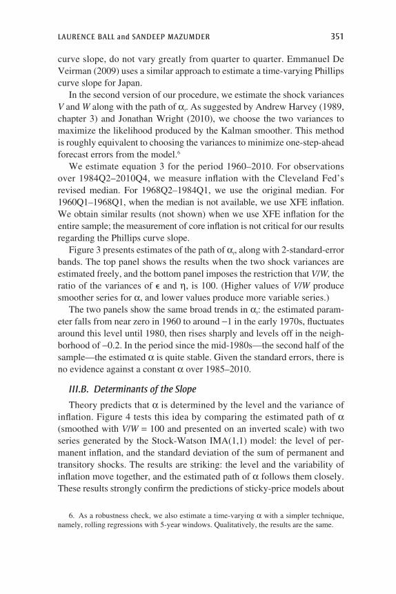
Theory predicts that a is determined by the level and the variance of inflation. Figure 4 tests this idea by comparing the estimated path of a (smoothed with V/W = 100 and presented on an inverted scale) with two series generated by the Stock-Watson IMA(1,1) model: the level of per-manent inflation, and the standard deviation of the sum of permanent and transitory shocks. The results are striking: the level and the variability of inflation move together, and the estimated path of a follows them closely. These results strongly confirm the predictions of sticky-price models about
6. As a robustness check, we also estimate a time-varying a with a simpler technique, namely, rolling regressions with 5-year windows. Qualitatively, the results are the same.

352 Brookings Papers on Economic Activity, spring 2011
time variation in a. In particular, the high and variable inflation of the 1970s and early 1980s created a steep Phillips curve; the curve was flatter before 1973 and after the Volcker disinflation, when inflation was relatively low and stable.
We can also capture these ideas with a regression. We assume that the coefficient a is a linear function of the other two series in figure 4:
Figure 3. estimated Time-Varying phillips curve slopes, 1960Q1–2010Q4a
No restriction on shock variances
1.0
–0.5
–2.0
197519701965 1980 1985 19951990 2000 2005 2010
Source: Authors’ calculations. a. Estimated by equation 3 in the text using median inflation data from the Federal Reserve Bank of
Cleveland (original median for 1968Q2–1984Q1, revised median for 1984Q2–2010Q4) and XFE inflation data for 1960Q1–1968Q1. Dotted lines indicate 2-standard-error bands.
b. V and W are the variances of �t and η
t in equation 3, respectively.
Slope (α)
–1.5
197519701965 1980 1985 19951990 2000 2005 2010
–1.0
0
0.5
1.5
Shock variance V = 100Wb
Slope (α)
1.0
–0.5
–2.0
–1.5
–1.0
0
0.5
1.5

laurence ball and sandeep mazumder 353
at = (a0 + a1p–
t + a2st), where p– and s are the level of permanent inflation and the standard deviation of the sum of permanent and temporary shocks, respectively. Substituting this assumption into equation 3 yields
( ) *41
4 1 2 3 4 0
1
π π π π π
π
t t t t t ta u u
a
= + + +( ) + −( )
+
− − − −
tt t t t tu u a u u−( ) + −( ) +* * .2σ e
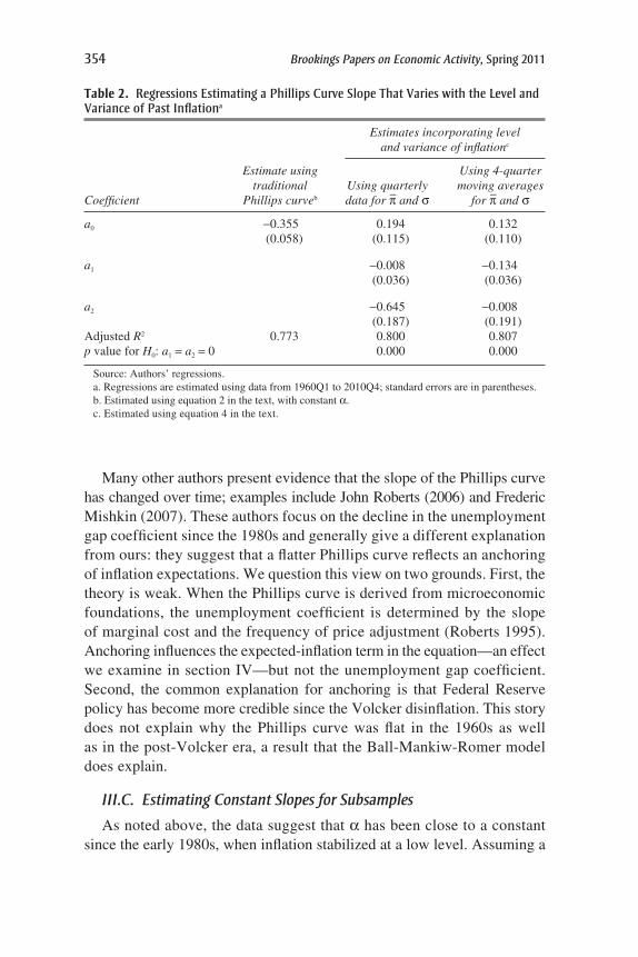
Table 2 presents estimates of this equation for 1960–2010 and compares them with estimates of an equation with a constant a. We measure p– t and st in two different ways: with the quarterly series for these parameters and with 4-quarter moving averages. In both cases the joint significance of the p– and s terms is high (p < 0.01). Unfortunately, the collinearity between the two variables makes it difficult to distinguish their individual roles: only p– is significant in one of our specifications, and only s is significant in the other.
Figure 4. permanent component of median consumer price Inflation and Time-Varying phillips curve slope, 1960–2010
14
8
2
0
–2
–0.2
0
–0.4
–0.6
–0.8
–1
–1.2
197519701965 1980 1985 19951990 2000 2005 2010
Source: Authors’ calculations. a. Calculated using Stock and Watson’s (2007) procedure for decomposing inflation into permanent
and transitory components. b. Standard deviation of the sum of permanent and transitory shocks. c. From figure 3, bottom panel.
Percent per year Slope (α)
4
6
10
12
16–1.4
Permanent componentof inflationa (left scale)
Standard deviationb × 10 (left scale)
Time-varying Phillips curveslopec (inverted, right scale)
354 Brookings Papers on Economic Activity, spring 2011
Many other authors present evidence that the slope of the Phillips curve has changed over time; examples include John Roberts (2006) and Frederic Mishkin (2007). These authors focus on the decline in the unemployment gap coefficient since the 1980s and generally give a different explanation from ours: they suggest that a flatter Phillips curve reflects an anchoring of inflation expectations. We question this view on two grounds. First, the theory is weak. When the Phillips curve is derived from microeconomic foundations, the unemployment coefficient is determined by the slope of marginal cost and the frequency of price adjustment (Roberts 1995). Anchoring influences the expected-inflation term in the equation—an effect we examine in section IV—but not the unemployment gap coefficient. Second, the common explanation for anchoring is that Federal Reserve policy has become more credible since the Volcker disinflation. This story does not explain why the Phillips curve was flat in the 1960s as well as in the post-Volcker era, a result that the Ball-Mankiw-Romer model does explain.
III.C. Estimating Constant Slopes for Subsamples
As noted above, the data suggest that a has been close to a constant since the early 1980s, when inflation stabilized at a low level. Assuming a
Table 2. regressions estimating a phillips curve slope That Varies with the level and Variance of past Inflationa
Estimatesincorporatinglevel andvarianceofinflationc
Estimateusing Using4-quarter traditional Usingquarterly movingaveragesCoefficient Phillipscurveb dataforp–ands forp–ands
a0 -0.355 0.194 0.132 (0.058) (0.115) (0.110)
a1 -0.008 -0.134 (0.036) (0.036)
a2 -0.645 -0.008 (0.187) (0.191)Adjusted R2 0.773 0.800 0.807p value for H0: a1 = a2 = 0 0.000 0.000
Source: Authors’ regressions.a. Regressions are estimated using data from 1960Q1 to 2010Q4; standard errors are in parentheses.b. Estimated using equation 2 in the text, with constant a.c. Estimated using equation 4 in the text.

laurence ball and sandeep mazumder 355
constant a will make it easier to enrich the model along other dimensions. Therefore, we assume a constant a starting in 1985Q1, roughly the end of the disinflation and high unemployment of the early 1980s. We examine periods ending in 2007Q4 and 2010Q4 to check for effects of the Great Recession.7
For comparison, we also estimate a constant a for the periods 1960–72 and 1973–84. Figure 4 suggests some variation in a within these periods, but the statistical significance of this variation is borderline. a is generally low in absolute value during the first period and high during the second.
Table 3 presents estimates of a for each of the four periods. We estimate equations with the output gap as well as with the unemployment gap, and with XFE inflation as well as with median inflation. For the first period, 1960–72, we examine only XFE inflation, because median inflation is not available for most of the period. We measure median inflation with the original Cleveland Fed series for 1973–84 and with the revised series for the periods beginning in 1985.8
For the first three time periods in the table, covering the years from 1960 to the eve of the financial crisis, the estimated coefficients are similar for the two inflation measures. The coefficient on the unemployment gap is around -0.2 or -0.25 for both 1960–72 and 1985–2007. The coefficient is around -0.7 for the 1973–84 period of high and volatile inflation. The coefficients on the output gap are about -0.5 times the unemployment coefficients, as suggested by Okun’s Law.
As before, multiplying the output coefficient by 1.6 yields the long-run effect on inflation of a 1-percentage-point output gap for a year. For 1985–2007, with inflation measured by the median, this effect is (1.6)(0.11) = 1.76. The sacrifice ratio is 1/(0.176), or about 6.
Extending the final sample from 2007 to 2010 has different effects for the different core inflation measures. For XFE inflation, the coefficients decline substantially in absolute value; for median inflation, the coefficients fall by less (when activity is measured by the unemployment gap) or not at all (for the output gap). This difference suggests greater stability in the Phillips curve when inflation is measured by the median, a result we will confirm with dynamic forecasts.
7. The results do not change significantly when we start the sample a year or two later. They are less robust when we move the start date earlier, with observations before 1985 proving influential.
8. Note that in these regressions we use the original median through 1984 even though the revised median is available starting in 1983Q2. This choice ensures that our measure of median inflation is consistent over the 1973–84 subsample.

356 Brookings Papers on Economic Activity, spring 2011
III.D. The Great Recession and the Risk of Deflation
We now revisit the puzzle of inflation over 2008–10. Figure 5 presents dynamic forecasts of quarterly inflation based on the unemployment and output gaps over that period and estimated Phillips curves for 1985–2007. Inflation is measured by the median in the top two panels and by XFE in the bottom two panels. Figure 6 shows 4-quarter averages of actual and
Table 3. regressions estimating a constant phillips curve slope in different subperiodsa
Estimatesusingthe unemploymentgap Estimatesusingtheoutputgapb
Subperiodand Measuring Measuring Measuring Measuringindependent inflationas inflationas inflationas inflationasvariable medianinflationc XFEinflation medianinflation XFEinflation
1960Q1–1972Q4d
Unemployment -0.231 0.135 or output gap (0.103) (0.056)Adjusted R2 0.729 0.733Standard error 0.992 0.985 of regression
1973Q1–1984Q4Unemployment -0.650 -0.688 0.365 0.371 or output gap (0.172) (0.184) (0.095) (0.103)Adjusted R2 0.513 0.402 0.516 0.391Standard error 2.254 2.408 2.247 2.429 of regression
1985Q1–2007Q4Unemployment -0.202 -0.246 0.114 0.136 or output gap (0.054) (0.067) (0.029) (0.037)Adjusted R2 0.700 0.761 0.703 0.763Standard error 0.425 0.529 0.423 0.528 of regression
1985Q1–2010Q4Unemployment -0.168 -0.136 0.114 0.092 or output gap (0.031) (0.039) (0.019) (0.024)Adjusted R2 0.781 0.764 0.792 0.769Standard error 0.448 0.570 0.437 0.563 of regression
Source: Authors’ regressions.a. Estimated using equation 2 in the text. Standard errors are in parentheses.b. The output gap (y - y*)t (the logarithm of real GDP minus the logarithm of the Congressional Budget
Office’s estimate of potential real GDP) is substituted for the unemployment gap.c. Original median for 1973–84, revised median for 1985–2010, from the Federal Reserve Bank of
Cleveland.d. Estimates using median inflation are not presented for this period because data are unavailable before
1967Q2.

laurence ball and sandeep mazumder 357
forecast inflation, again as measured both by the median (top panel) and by XFE (bottom panel).
The forecasts for median inflation in the two figures are close to actual inflation over 2008–10; in contrast to figure 1, there is no missing deflation. The most important reason for this change in results is our allowance for
Figure 5. dynamic Forecasts of core consumer price Inflation, 2008–10, based on phillips curve estimates for 1985–2007a
Median inflation
Actual
Using unemployment gap Percent
Source: Authors’ calculations. a. Forecasts are derived from equation 2 using quarterly data for the period 1985Q1–2007Q4. Dotted
lines indicate 2-standard-error bands.
2002 2004 2006 2008 2010
–2
–1
0
1
2
3
4
–3
Using output gap Percent
2002 2004 2006 2008 2010
–2
–1
0
1
2
3
4
–3
XFE inflation Using unemployment gap
Percent
2002 2004 2006 2008 2010
–2
–1
0
1
2
3
4
–3
Using output gap Percent
2002 2004 2006 2008 2010
–2
–1
0
1
2
3
4
–3
Dynamic forecast
Actual
Dynamic forecast
Actual
Dynamic forecast
Actual
Dynamic forecast

358 Brookings Papers on Economic Activity, spring 2011
time variation in the Phillips curve slope. The output and unemployment coefficients for 1985–2007 are less than half as large as the estimates for the entire 1960–2007 period, which includes the high and unstable inflation of 1973–84. Smaller coefficients mean a smaller predicted fall in inflation.
How core inflation is measured is also important. The forecasts of XFE inflation in figures 5 and 6 fall to around -1 percent at the end of 2010, significantly below actual inflation. Forecast XFE inflation falls further
Figure 6. dynamic Forecasts of core consumer price Inflation, 4-Quarter moving averages, 2008–10a
Median inflation
Source: Authors’ calculations.a. Forecasts are derived from equation 2 using data for the period 1985Q1–2007Q4.
XFE inflationPercent per year
1.0
–1.0
–0.5
0
0.5
1.5
2.0
2.5
3.0
Percent per year
Actual
Forecast from output gap
Forecast from unemployment gap
1.0
–1.0
2003200220012000 2004 2005 20072006 2008 2009 2010
2003200220012000 2004 2005 20072006 2008 2009 2010
–0.5
0
0.5
1.5
2.0
2.5
3.0
Actual
Forecast from output gap
Forecast from unemployment gap

laurence ball and sandeep mazumder 359
than forecast median inflation because XFE inflation starts at a lower level in 2007. In addition, the estimated coefficients on the unemployment and output gaps are somewhat larger for XFE over 1985–2007.
If our Phillips curve for median inflation fits recent history, what does it imply for future inflation? We address this question with new dynamic forecasts based on estimates of the equation from 1985 through 2010. In this exercise we assume that unemployment and its natural rate follow the paths forecast by the CBO for 2011–13: unemployment is 9.4 percent in 2011, 8.4 percent in 2012, and 7.6 percent in 2013, and the natural rate is constant at 5.2 percent. We also compute dynamic forecasts based on CBO forecasts of the output gap over 2011–13.
Figure 7 shows 4-quarter moving averages of the resulting forecasts. Because unemployment remains above the natural rate and output is below potential, inflation falls steadily. It becomes negative at the end of 2011, and at the end of 2013 it reaches -1.9 percent (based on the unemployment gap forecasts) or -1.3 percent (based on the output gap forecasts). Thus, our Phillips curve, which explains why deflation has not occurred yet, also predicts that deflation will arrive soon.
Figure 7. dynamic Forecasts of median consumer price Inflation, 2011–13a
Source: Authors’ calculations.a. Actual data and forecasts are 4-quarter moving averages. Forecasts are derived from equation 2
using data for the period 1985Q1–2010Q4. b. Assumes that the output gap follows the path forecast by the CBO for 2011–13.c. Assumes that unemployment and its natural rate follow the paths forecast by the CBO for 2011–13:
unemployment is 9.4 percent in 2011, 8.4 percent in 2012, and 7.6 percent in 2013, and the natural rate is constant at 5.2 percent.
Percent per year
Actual
Forecast fromoutput gapb
Forecast from unemployment gapc
1.0
–1.0
–1.5
200320022001 2004 2005 20072006 2008 2009 2010 2011 2012 2013
–0.5
0
0.5
1.5
2.0
2.5
3.0
360 Brookings Papers on Economic Activity, spring 2011
III.E. Robustness
We have checked the robustness of our results along several dimensions. Specifically, we
—add lags of unemployment and longer lags of inflation to the Phillips curve model, as suggested by Gordon (2011)
—include Stock and Watson’s (2010) unemployment recession gap variable (the difference between current unemployment and minimum unemployment over the current and previous 11 quarters) as an additional activity measure
—substitute Guy Debelle and Douglas Laxton’s (1997) nonlinear trans-formation of unemployment as the activity measure
—add Ball and Robert Moffitt’s (2002) measure of the acceleration of productivity growth to the model
—estimate a path of the natural rate u* jointly with the coefficient on the Phillips curve, rather than rely on CBO estimates of u*
—estimate an equation for total inflation that includes a measure of supply shocks (the difference between total inflation and median inflation), rather than estimate an equation for core inflation.
None of these extensions has a significant impact on our conclusions. The appendix to this paper provides details.
IV. Anchored Expectations?
So far we have estimated Phillips curves based on the assumption that expected inflation equals past inflation. A growing number of economists, including Mishkin (2007), Bernanke (2010), and Donald Kohn (2010), argue that this assumption, although once acceptable, has become untenable. In their view, the public’s growing understanding that the Federal Reserve is committed to low and stable inflation has “anchored” expectations, so that they therefore no longer respond strongly to past inflation. Here we review past evidence on the anchoring of expectations and present new evidence. We also examine the importance of anchoring for explaining inflation during the Great Recession and for forecasting future inflation.
We distinguish between two kinds of anchoring: “shock anchoring” and “level anchoring.” The first means that transitory shocks to inflation are not passed into expectations or into future inflation. The second means that expectations are tied to a particular level of inflation, such as 2 percent. We find strong evidence for shock anchoring since the early 1980s. Level anchoring has occurred gradually and is incomplete, yet it may strongly influence future inflation.

laurence ball and sandeep mazumder 361
IV.A. Shock Anchoring
A consensus (including, for example, Taylor 1999 and Clarida and others 2000) holds that the United States experienced a shift in monetary regime during Paul Volcker’s tenure as Federal Reserve chairman. Before Volcker, the Federal Reserve accommodated supply shocks, and price set-ters recognized this behavior. A shock that raised inflation raised expected inflation, which fed into future inflation, and the Federal Reserve did not systematically oppose this process. Since Volcker, however, the Federal Reserve has been committed to stable inflation. As a result, supply shocks do not strongly affect expectations or future inflation. Expectations have become shock anchored.9
Previous empirical work presents evidence of shock anchoring. Sommer (2004), for example, finds that supply shocks, measured either by changes in food and energy prices or by asymmetries in price distributions, have strong effects on inflation and on survey expectations of inflation before 1979, but little effect afterward. Authors such as Hooker (2002) and Fuhrer and others (2009) report similar results.
We confirm these findings with the exercise reported in table 4. We esti-mate Phillips curves in which core inflation depends on the unemployment
9. Christiano and Gust (2000) formalize these ideas with a model of the “expectations trap.”
Table 4. regressions estimating the phillips curve with shock anchoringa
Estimationperiod
Independentvariable 1960Q1–1972Q4 1973Q1–1984Q4 1985Q1–2010Q4
EstimatesusinglaggedcoreinflationUnemployment gap -0.231 -0.650 -0.168 (0.103) (0.172) (0.031)Adjusted R2 0.729 0.513 0.781
EstimatesusinglaggedtotalinflationUnemployment gap -0.319 -0.620 -0.003 (0.091) (0.165) (0.064)Adjusted R2 0.789 0.551 0.042
EstimatesusinglaggedcoreandlaggedtotalinflationUnemployment gap -0.329 -0.630 -0.150 (0.095) (0.165) (0.031)Weight on lagged -0.117 0.326 0.886 core inflation (0.295) (0.294) (0.046)Adjusted R2 0.785 0.553 0.791
Source: Authors’ regressions.a. Core inflation is XFE inflation for 1960Q1–1972Q4 and median inflation for 1973Q1–2010Q4.

362 Brookings Papers on Economic Activity, spring 2011
gap and lagged inflation, but we compare two versions of lagged inflation: lagged core inflation and lagged total inflation. We interpret total inflation as the sum of core inflation and supply shocks. We measure core inflation with median inflation for the periods 1973–84 and 1985–2010, and with XFE inflation for 1960–72.
The results are stark. For 1960–72 and 1973–84, the adjusted R2 of the Phillips curve is higher when it includes lagged total inflation. When both lagged total and lagged core inflation are included, the weight on the latter is insignificant in both periods. For 1985–2010, these results are reversed. The estimated weight on lagged core inflation is 0.89.
For 1985–2010 we also examine the behavior of expected inflation as measured by 1-year forecasts from the Survey of Professional Forecasters (SPF), which are not available for earlier periods. We regress expected inflation on an average of lagged core inflation and lagged total inflation and find a weight on the former of 0.86 (with a standard error of 0.06; results not shown).
Finally, for 1985–2010 we experiment with time-varying weights on lagged core and lagged total inflation. We find little variation: in equations for both actual and expected inflation, the weights on lagged core inflation are consistently close to 1 (results not shown). Shock anchoring is a stable feature of the post-Volcker monetary regime.
IV.B. Level Anchoring
Many recent discussions of anchoring suggest that expected inflation in the United States is tied to a particular level: specifically, 2 percent per year. Economists such as Mishkin (2007) argue that the Federal Reserve is committed to keeping inflation close to 2 percent and that the public has come to understand this fact. This anchoring of expectations pushes actual inflation toward 2 percent as well.
More precisely, Mishkin suggests that expectations of core PCE infla-tion are anchored at 2 percent. Since 1980, core CPI inflation has exceeded core PCE inflation by about 0.5 percentage point on average (for both the weighted median and the XFE measures of core inflation). We should expect, therefore, that expectations of core CPI inflation are anchored at 2.5 percent.
Using rolling regressions, Williams (2006) and Fuhrer and Olivei (2010) find that the coefficients on inflation lags in the Phillips curve, when not constrained to sum to 1, have fallen over time. This finding is consistent with level anchoring of expectations. We add to this evidence by estimat-

laurence ball and sandeep mazumder 363
ing the degrees of anchoring of both expected and actual inflation and how these parameters have evolved over time. One innovation is that we impose a specific level, 2.5 percent, at which inflation is anchored if it is anchored at all.
Whereas shock anchoring dates back to the Volcker regime shift, level anchoring is more recent. The idea that the Federal Reserve has an inflation target around 2 percent was first discussed in the early 1990s (for example, by Taylor 1993) and slowly became more prominent. To capture this history, we use data from 1985 through 2010 to estimate
( ) .5 2 5 11
4 1 2 3 4π δ δ π π π πte
t t t t t t= + −( ) + + +( ) +− − − − ee t ,
where dt follows a random walk. Expected inflation is thus a weighted average of lagged inflation and 2.5 percent, with time-varying weights. When d = 0, expectations are purely backward looking; when d = 1, expec-tations are fully anchored at 2.5 percent.
To estimate equation 5, we measure pe with SPF forecasts of inflation over the next 4 quarters. We measure past inflation with the Cleveland Fed median. We estimate the path of dt using the Kalman smoother, assuming that the variance of e is 100 times the variance of innovations in d.
The top panel of figure 8 presents our estimated series for dt. We find that dt is near zero until the early 1990s and then rises. It is around 0.6 over 2007–10. Expectations have become largely but not completely anchored.
We next examine the behavior of actual inflation. We assume that inflation depends on expected inflation and the unemployment gap, as in equation 1, and substitute in equation 5 for expected inflation. The result is
( ) *.6 2 5 11
4 1 2 3 4π δ δ π π π πt t t t t t t= + −( ) + + +( ) +− − − − αα u ut t−( ) + e .
We estimate this equation and a variation in which the output gap replaces the unemployment gap. The bottom two panels of figure 8 show the estimated path of dt for these specifications. Once again, d is near zero until the early 1990s and then rises. According to these results, as inflation expectations have become anchored, so has actual inflation.
The value of d in 2010Q4, the end of the sample, is 0.47 when the Phillips curve includes the unemployment gap, and 0.30 with the output gap. These values indicate a smaller degree of anchoring than we estimated for SPF

Figure 8. level anchoringa
Expected inflation
Source: Authors’ calculations.a. Series are calculated from estimates of equation 5 (top panel) and equation 6 (bottom two panels) in
the text, using quarterly data over 1985Q1–2010Q4. Expected inflation is measured as the SPF forecast of inflation over the next 4 quarters. Actual inflation is measured as median inflation from the Federal Reserve Bank of Cleveland. The path of δ
t is calculated using the Kalman smoother, assuming that the
variance of � is 100 times the variance of innovations in δ. Dotted lines show 2-standard-error bands.b. Weight on the argument in equation 5 or 6 that represents level anchoring at 2.5 percent per year.
Anchoring parameter δb
–0.6
19981995199219891986 2001 2004 2007
19981995199219891986 2001 2004 2007
19981995199219891986 2001 2004 2007
–0.4
0
–0.2
0.2
0.4
0.6
0.8
–0.6
–0.4
0
–0.2
0.2
0.4
0.6
0.8
Actual inflation, model with unemployment gapAnchoring parameter δb
–0.6
–0.4
0
–0.2
0.2
0.4
0.6
0.8
Actual inflation, model with output gapAnchoring parameter δb

laurence ball and sandeep mazumder 365
expectations in the top panel of figure 8. One possible explanation is that the expectations that enter the Phillips curve are those of typical price setters, who are less sophisticated than professional forecasters and therefore learn more slowly about the Federal Reserve’s commitment to 2.5 percent infla-tion. But one should not make too much of the differences across panels in figure 8, because the confidence intervals for the ds overlap.
Our estimates of the coefficient a in equation 6 are -0.24 (standard error = 0.03) for the unemployment gap and 0.13 (standard error = 0.02) for the output gap. These estimates are somewhat larger in absolute value than the as for our basic Phillips curve, which includes lagged inflation with a coefficient of 1, but again the confidence intervals overlap.
IV.C. Dynamic Forecasts
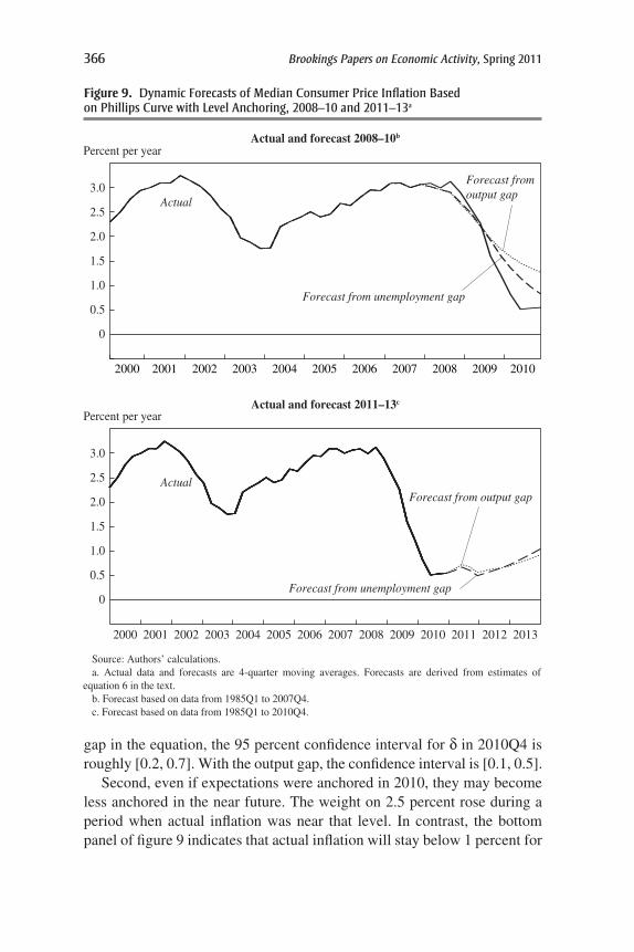
We now revisit the behavior of inflation in the recent past and its likely future behavior. The top panel of figure 9 parallels the top panel of figure 6: it presents dynamic forecasts of 4-quarter-moving-average inflation over 2008–10, based on estimates of equation 6 for 1985–2007. We assume that, throughout 2008–10, the anchoring parameter d remains at the levels estimated for 2007Q4: 0.31 when the equation includes the unemployment gap and 0.26 when it includes the output gap. In the figure, forecast infla-tion falls less than actual inflation over 2008–10. The forecasts from our purely backward-looking equation in the top panel of figure 6 are closer to actual inflation. This difference in forecast performance, however, is modest in size and statistically insignificant: accounting for anchoring does not sharply change inflation forecasts for the last few years. This finding reflects the fact that the estimated degree of anchoring in 2007Q4 is fairly small. In addition, inflation has been fairly close to 2.5 percent, so that forecasts are not sensitive to the weights on 2.5 percent and lagged inflation.
The bottom panel of figure 9 parallels figure 7 for our Phillips curve without anchoring. It shows forecasts of 4-quarter-moving-average infla-tion over 2011–13 based on estimates of equation 6 for 1985–2010. Here we assume that d stays at the level estimated for 2010Q4. In this exercise, anchoring makes a big difference. Deflation, which is predicted by our basic Phillips curve, does not occur in our forecasts with anchoring. Instead, infla-tion is steady at about 0.5 percent and then rises to 1 percent at the end of 2013. Partial anchoring pulls expected inflation up toward 2.5 percent, and that causes actual inflation to bottom out rather than fall in response to high unemployment.
Two caveats are in order. First, there is considerable uncertainty about the degree of anchoring in the Phillips curve. With the unemployment
366 Brookings Papers on Economic Activity, spring 2011
gap in the equation, the 95 percent confidence interval for d in 2010Q4 is roughly [0.2, 0.7]. With the output gap, the confidence interval is [0.1, 0.5].
Second, even if expectations were anchored in 2010, they may become less anchored in the near future. The weight on 2.5 percent rose during a period when actual inflation was near that level. In contrast, the bottom panel of figure 9 indicates that actual inflation will stay below 1 percent for
Figure 9. dynamic Forecasts of median consumer price Inflation based on phillips curve with level anchoring, 2008–10 and 2011–13a
Actual and forecast 2008–10b
Source: Authors’ calculations.a. Actual data and forecasts are 4-quarter moving averages. Forecasts are derived from estimates of
equation 6 in the text.b. Forecast based on data from 1985Q1 to 2007Q4.c. Forecast based on data from 1985Q1 to 2010Q4.
Actual and forecast 2011–13c
Percent per year
Percent per year
Actual
Forecast fromoutput gap
Forecast from unemployment gap1.0
0
0.5
1.5
2.0
2.5
3.0
ActualForecast from output gap
Forecast from unemployment gap
1.0
2000
0
0.5
1.5
2.0
2.5
3.0
2000 2001 2002 2003 2004 2005 2006 2007 2008 2009 2010
200320022001 2004 2005 20072006 2008 2009 2010 2011 2012 2013

laurence ball and sandeep mazumder 367
several years but that expectations will still be tied to 2.5 percent. That suggests suboptimal forecasting. Price setters may learn that inflation is stuck below 2.5 percent, and expectations will adjust downward.
Believers in anchoring point out that long-run inflation expectations—as measured, for example, by 10-year SPF forecasts—have been close to 2.5 percent since 2000. It is plausible that these expectations will remain anchored in the future, because the public believes that the Federal Reserve will manage eventually to return inflation to its 2.5 percent target. How-ever, in most theories of the Phillips curve—both sticky-price and sticky-information models—prices depend on expected inflation over the period when the prices are likely to be in effect. This period is on the order of 1 year rather than 10 years. Recent empirical work also finds that actual inflation depends on 1-year rather than 10-year SPF expectations (Fuhrer 2011).
The forecasts of inflation in the bottom panel of figure 9 are fairly close to those of others. At the beginning of 2011, the CBO was forecasting annual core CPI inflation rates of 0.9, 1.0, and 1.4 percent over 2011–13. These fore casts are 0.3 to 0.5 percentage point above ours. These differences might be explained by the different definitions of core inflation used: median for us and XFE for the CBO (although it is not obvious that forecasts of either should be higher than the other). The SPF median forecast for XFE infla-tion is 1.3 percent for 2011 and 1.7 percent for 2012 (forecasts for 2013 are unavailable). The forecast for 2012 is a full percentage point above ours. One factor here is that only 44 percent of SPF forecasters say they use the concept of the natural rate of unemployment. Evidently, many forecasters use models of inflation that differ greatly from the Phillips curves we estimate.
V. The New Keynesian Phillips Curve
We have followed an empirical tradition that assumes that expected inflation is determined by past inflation and possibly the central bank’s inflation target. Another literature studies Phillips curves based on rational expec-tations. The foundation for much of this work is the “New Keynesian Phillips curve” (NKPC) derived from Calvo’s (1983) model of staggered price adjustment. The original version of this equation, as presented by Roberts (1995), was
( ) * ,7 1π π λt t t ty y= + −( )+E
where Etpt+1 is this quarter’s rational forecast of next quarter’s inflation and y - y* is the output gap.

368 Brookings Papers on Economic Activity, spring 2011
A number of authors (for example, Galí and Gertler 1999, Mankiw 2001) show that this Phillips curve fits the data poorly. To understand this result, rearrange equation 7 to obtain
( ) * .8 1E t t t ty yπ π λ+ − = − −( )
The theory behind the NKPC implies that the parameter l is positive. Therefore, equation 8 says that the output gap in quarter t has a negative effect on the expected change in inflation from t to t + 1. In the data, output has a positive correlation with the change in inflation—both before the Great Recession and during it, when output was low and inflation fell. As a result, estimates of l are consistently negative, contradicting the theory.
Motivated by this finding, Galí and Gertler modify the NKPC by replac-ing the output gap with real marginal cost mc:
( ) .9 1π π λt t t tmc= ++E
Galí and Gertler measure real marginal cost with real unit labor costs, also known as labor’s share of income. They obtain a positive estimate of l, a result that has led many researchers to adopt their specification.
Jeremy Rudd and Karl Whelan (2005, 2007) and Mazumder (2010) criticize Galí and Gertler’s work, arguing that labor’s share of income is not a credible measure of real marginal cost. Labor’s share is generally counter cyclical, and there is a strong case for marginal cost being pro-cyclical, on the basis of both theory and evidence, such as Mark Bils’s (1987) and Mazumder’s studies of overtime labor. Mazumder estimates equation 9 with a procyclical measure of marginal cost based on overtime and obtains negative estimates of l—the same result that discredited the original NKPC.10
Despite skepticism about the NKPC, we ask whether it helps explain inflation during the Great Recession. It does not; indeed, recent experi-ence provides a new reason to doubt the model. The problem is different from the one stressed in previous work: the Galí-Gertler specification does not fit recent data even if we accept their measure of marginal cost.
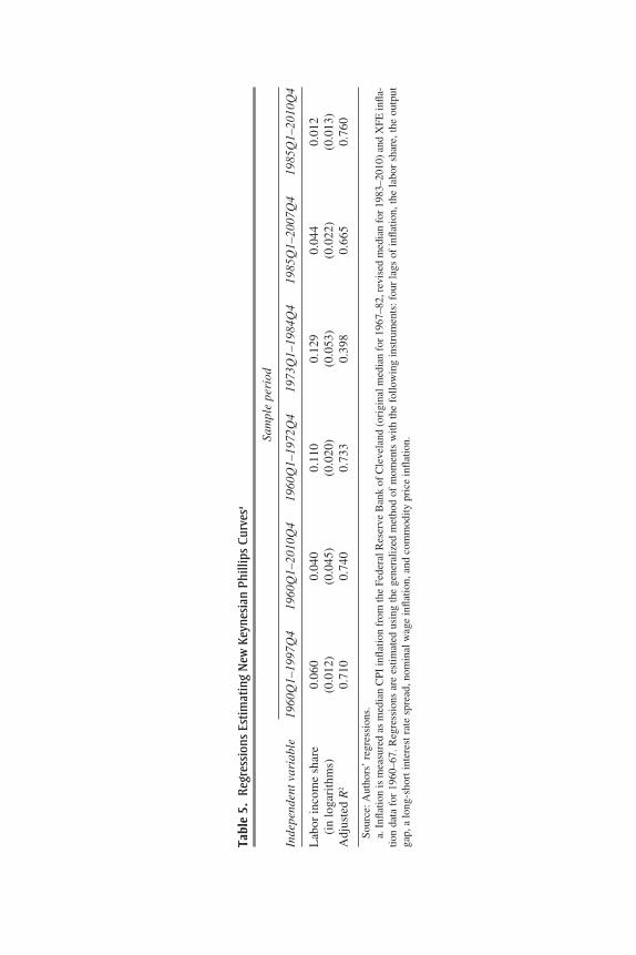
Table 5 presents estimates of the parameter l in the NKPC, with mar-ginal cost measured by labor’s share. We estimate the equation using the
10. Rudd and Whelan, as well as Kleibergen and Mavroeidis (2009), also demonstrate technical problems, such as weak instruments, with the studies supporting the Galí-Gertler model.
Tabl
e 5.
reg
ress
ions
est
imat
ing
new
Key
nesi
an p
hilli
ps c
urve
sa
Sa
mpl
epe
riod
Inde
pend
entv
aria
ble
1960
Q1–
1997
Q4
1960
Q1–
2010
Q4
1960
Q1–
1972
Q4
1973
Q1–
1984
Q4
1985
Q1–
2007
Q4
1985
Q1–
2010
Q4
Lab
or in
com
e sh
are
0.06
0 0.
040
0.11
0 0.
129
0.04
4 0.
012
(i
n lo
gari
thm
s)
(0.0
12)
(0.0
45)
(0.0
20)
(0.0
53)
(0.0
22)
(0.0
13)
Adj
uste
d R
2 0.
710
0.74
0 0.
733
0.39
8 0.
665
0.76
0
Sour
ce: A
utho
rs’
regr
essi
ons.
a. I
nflat
ion
is m
easu
red
as m
edia
n C
PI in
flatio
n fr
om th
e Fe
dera
l Res
erve
Ban
k of
Cle
vela
nd (
orig
inal
med
ian
for
1967
–82,
rev
ised
med
ian
for
1983
–201
0) a
nd X
FE in
fla-
tion
data
for
196
0–67
. Reg
ress
ions
are
est
imat
ed u
sing
the
gene
raliz
ed m
etho
d of
mom
ents
with
the
follo
win
g in
stru
men
ts: f
our
lags
of
infla
tion,
the
labo
r sh
are,
the
outp
ut
gap,
a lo
ng-s
hort
inte
rest
rat
e sp
read
, nom
inal
wag
e in
flatio
n, a
nd c
omm
odity
pri
ce in
flatio
n.

370 Brookings Papers on Economic Activity, spring 2011
generalized method of moments (GMM) with the following orthogonal-ity condition:
( ) ,10 01Et t t t tmcπ λ π− −( ){ } =+ z
where zt is a vector of variables dated t and earlier; thus, these variables are orthogonal to the inflation surprise in t + 1. We use the same instruments as Galí and Gertler: four lags each of inflation, labor’s share, the output gap, the spread between long- and short-term interest rates, nominal wage infla-tion, and commodity price inflation. We use the median CPI inflation rate, but the results are similar for other inflation measures (including that used by Galí and Gertler, the GDP deflator).
As in previous parts of this paper, we find that the coefficient in the Phillips curve varies across time periods. Galí and Gertler report a sig-nificantly positive coefficient for 1960–97, which fits theory, and which we replicate. The noteworthy result in table 5 is that the coefficient on labor’s share is significantly positive for the period 1985–2007 (t= 2.04), but insignificant for 1985–2010 (t = 0.92). In other words, the model’s fit deteriorates when we add 2008–10 to the sample.
Figure 10 shows why. For 1985–2010 it plots annual averages of labor’s share of income against the unemployment gap. We see that 2009 and 2010 are big outliers. Before then, labor’s share was positively correlated with the unemployment gap—as noted before, it was countercyclical. This is an unappealing feature in a marginal cost measure, but it produces a positive estimate of l. The Great Recession, unlike previous recessions, has been accompanied by a sharp fall in labor’s share: for whatever reason, produc-tivity growth was strong and real wages did not keep up. This change in cyclicality changes the estimate of the Phillips curve coefficient.
To see the problem in a different way, we substitute mc for the output gap in equation 8:
( ) .11 1Et t t tmcπ π λ+ − = −
This version of Galí and Gertler’s equation says that the expected change in inflation depends negatively on labor’s share. Throughout 2009 and 2010, when labor’s share was lower than average, the equation says that inflation was expected to rise. In fact, inflation fell, and it seems dubious that price setters repeatedly expected the opposite, that inflation would rise during

laurence ball and sandeep mazumder 371
the Great Recession. In any case, in quarterly data, falling inflation and expectations of rising inflation imply repeated forecast errors in the same direction, a violation of rational expectations.
VI. Conclusion
This paper has examined U.S. inflation from 1960 through 2010. We find that a simple accelerationist Phillips curve fits the entire period, including the recent Great Recession, under two conditions: we measure core inflation with the weighted median of price changes, and we allow the slope of the Phillips curve to change with the level and variance of inflation. Both of these ideas are motivated by models of costly price adjustment.
We also find evidence of a change in the Phillips curve since the 1990s: expectations of inflation, and hence actual inflation, have become partially anchored at a level of 2.5 percent. If this anchoring persists, the United States is likely to avoid deflation in the near future, despite high unemploy-ment. Deflation may occur, however, if low inflation leads to a deanchoring of expectations.
We conclude by highlighting a topic for future research, namely, the effect of unemployment duration on the Phillips curve. Ricardo Llaudes (2005)
Figure 10. labor Income share and the unemployment Gap, 1985–2010a
Source: Bureau of Labor Statistics and Congressional Budget Office data.a. Data are annual averages.
Labor share, 1992 = 100
Unemployment gap (percentage points)
2008
2009
2010
100
0–1 1 2 3 4
96
98
102
104
106

372 Brookings Papers on Economic Activity, spring 2011
finds, for a number of countries, that long-term unemployment (the fraction of the labor force unemployed for 1 year or longer) puts less downward pressure on inflation than short-term unemployment. It is difficult to test this idea with U.S. data because long-term and short-term unemployment are highly collinear. This collinearity is diminishing, however, because long-term unemployment has risen much more than short-term unemploy-ment since 2008. We may soon have enough data to tell whether long-term unemployment has less effect on inflation. If it does, then inflation will fall by less over the next few years than one would expect based on aggregate unemployment. The shift toward long-term unemployment, along with expectations anchoring, could prevent deflation.
a p p e n d I X
Robustness Tests
Here we briefly discuss five variations to our preferred Phillips curve specification that we also test for robustness.
Longer Lags
Gordon (2011) argues that the Phillips curve fits history better if it includes lags of the unemployment gap and long lags of inflation. Following Gordon, we modify the basic Phillips curve in equation 1 by including 4 lags of the unemployment gap and 24 lags of inflation (with the sum of the coefficients on the inflation lags set to 1). We continue to measure inflation with the Cleveland Fed median. When we estimate this specification for the period 1960–2007,11 the sum of unemployment gap coefficients is -0.26. Paralleling the top panel of figure 6, figure A1 shows dynamic forecasts of 4-quarter inflation over 2008–10. The forecast for 2010Q4 is -5.1 percent. Thus, our finding that the pre-2008 Phillips curve incorrectly predicts deflation is robust to the equation’s lag structure.
The Stock-Watson Unemployment Gap
Stock and Watson (2010) compute a new unemployment gap variable defined as the difference between the unemployment rate in quarter t and the minimum unemployment rate from quarters t to t - 11:
( ) min , . . . , .A SW1 11u u u ut t t t= − ( )−
11. Data on core inflation start in 1957; therefore, this regression actually starts in 1964.

laurence ball and sandeep mazumder 373
Computing the gap variable in this way focuses on recessions by producing only nonnegative values for the unemployment gap. The first two panels of table A1 compare the results of our preferred Phillips curve specification for the CBO unemployment gap and the Stock-Watson unemployment gap. These results show that a very similar Phillips curve is produced whichever measure of the unemployment gap is used in the model. We then estimate a version of the Phillips curve that incorporates both unemployment gap variables simultaneously:
( )A21
4
1
1 2 3 4
0 1 2
π π π π π
β β β
t t t t t
tD D
= + + +( )
+ + +
− − − −
22t t t tu u u( ) −( ) + +* ,λ SW e
where D1t is a dummy variable equal to 1 for 1973Q1–2010Q4 and 0 otherwise, and D2t is a dummy variable equal to 1 for 1985Q1–2010Q4 and 0 otherwise. This model is estimated from 1960Q1 to 2010Q4 and allows us to compare the statistical significance of the two unemployment gap variables at the same time. Specifically, we estimate the model jointly while also imposing the restriction that the ratio of the coefficients on the
Source: Authors’ calculations.a. Actual data and forecasts are 4-quarter moving averages. Forecasts are derived from equation 2 plus
4 lags of the unemployment gap and 24 lags of inflation (where the coefficients on the inflation lags sum to 1), using data for 1960–2007.
Percent per year
Actual
Dynamic forecast
1
–1
–2
2003200220012000 2004 2005 20072006 2008 2009 2010
0
–3
–4
–5
2
3
Figure A1. dynamic Forecasts of median consumer price Inflation using additional unemployment Gap and Inflation lags, 2008–10a

374 Brookings Papers on Economic Activity, spring 2011
Table A1. Variations on the Traditional phillips curvea
Estimationperiod
Independentvariable 1960Q1–1972Q4 1973Q1–1984Q4 1985Q1–2010Q4
TraditionalPhillipscurveusingCBOunemploymentgapmeasureUnemployment gap -0.231 -0.650 -0.168 (0.103) (0.172) (0.031)Adjusted R2 0.729 0.513 0.781
TraditionalPhillipscurveusingStock-Watsonunemploymentgapmeasureb
Unemployment gap -0.296 -0.521 -0.157 (0.118) (0.164) (0.027)Adjusted R2 0.735 0.477 0.788
Nonlinear(Debelle-Laxton)Phillipscurvec
Unemployment gap -0.965 -5.836 -1.312 (0.390) (1.441) (0.241)Adjusted R2 0.734 0.529 0.780
PhillipscurveincludingproductivitygrowthUnemployment gap -0.224 -0.636 -0.158 (0.105) (0.172) (0.030)Productivity growth -0.014 -0.096 -0.049 (0.033) (0.085) (0.016)Adjusted R2 0.724 0.515 0.798
1973Q1–1984Q4 1985Q1–2007Q4 1985Q1–2010Q4
Phillipscurveincludingsupplyshocksd
Unemployment gap -0.667 -0.194 -0.167 (0.175) (0.055) (0.030)Supply shocke 0.852 1.031 1.038 (0.221) (0.034) (0.024)Adjusted R2 0.566 0.922 0.953
Source: Authors’ calculations.a. Except in the second and third panels, the unemployment gap is the difference between the actual
unemployment rate and the CBO measure of the natural rate of unemployment. Except in the bottom panel, inflation is XFE inflation for 1960Q1–1972Q4 and median CPI inflation from the Federal Reserve Bank of Cleveland thereafter.
b. The Stock-Watson unemployment gap is the difference between unemployment in quarter t and the minimum unemployment rate from quarter t to quarter t - 11.
c. The Debelle-Laxton unemployment gap is the ratio of the CBO unemployment gap (note a) to the actual unemployment rate.
d. The dependent variable is total CPI inflation, and lagged inflation on the right-hand side of the equa-tion is Cleveland Fed median CPI inflation.
e. Total CPI inflation minus median CPI inflation.
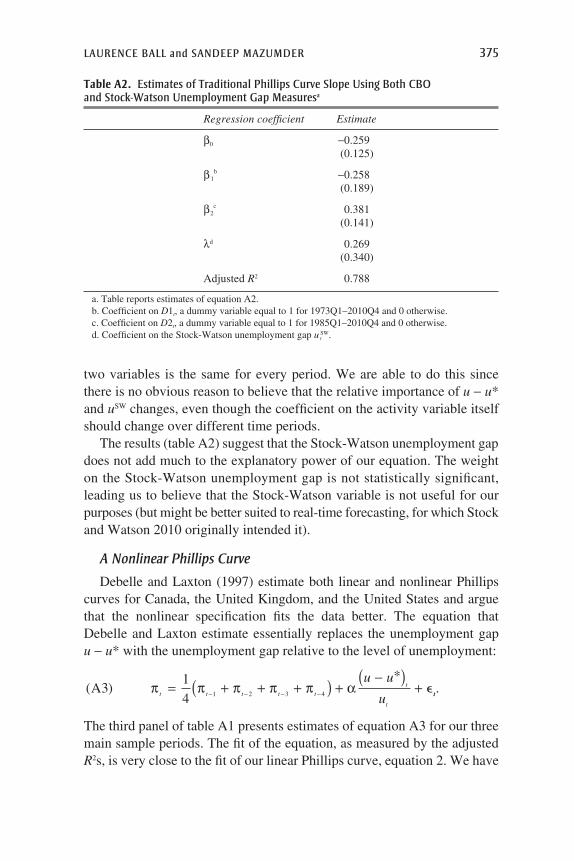
laurence ball and sandeep mazumder 375
two variables is the same for every period. We are able to do this since there is no obvious reason to believe that the relative importance of u - u* and uSW changes, even though the coefficient on the activity variable itself should change over different time periods.
The results (table A2) suggest that the Stock-Watson unemployment gap does not add much to the explanatory power of our equation. The weight on the Stock-Watson unemployment gap is not statistically significant, leading us to believe that the Stock-Watson variable is not useful for our purposes (but might be better suited to real-time forecasting, for which Stock and Watson 2010 originally intended it).
A Nonlinear Phillips Curve
Debelle and Laxton (1997) estimate both linear and nonlinear Phillips curves for Canada, the United Kingdom, and the United States and argue that the nonlinear specification fits the data better. The equation that Debelle and Laxton estimate essentially replaces the unemployment gap u - u* with the unemployment gap relative to the level of unemployment:
( )*
A31
4 1 2 3 4π π π π π αt t t t t
t
t
u u
u= + + +( ) +
−( )+− − − − e tt.
The third panel of table A1 presents estimates of equation A3 for our three main sample periods. The fit of the equation, as measured by the adjusted R2s, is very close to the fit of our linear Phillips curve, equation 2. We have
Table A2. estimates of Traditional phillips curve slope using both cbO and stock-Watson unemployment Gap measuresa
Regressioncoefficient Estimate
b0 -0.259 (0.125)
b 1b -0.258
(0.189)
b2c 0.381
(0.141)
ld 0.269 (0.340)
Adjusted R2 0.788
a. Table reports estimates of equation A2.b. Coefficient on D1t, a dummy variable equal to 1 for 1973Q1–2010Q4 and 0 otherwise.c. Coefficient on D2t, a dummy variable equal to 1 for 1985Q1–2010Q4 and 0 otherwise.d. Coefficient on the Stock-Watson unemployment gap u t
SW.

376 Brookings Papers on Economic Activity, spring 2011
also estimated a Phillips curve that includes both u - u* and (u - u*)/u (results not shown). In this case, high collinearity between the two variables causes both to be statistically insignificant. Thus, the data do not suggest that making the Phillips curve nonlinear improves the model.
When we estimate the Debelle-Laxton version of the Phillips curve for 1985–2007 and compute dynamic forecasts of inflation for 2008–10, the model performs less well than our linear specification. The actual 4-quarter moving average of median inflation fell from 3.1 percent to 0.5 percent from 2007Q4 to 2010Q4, whereas the Debelle-Laxton model predicts 4-quarter inflation of 1.3 percent in 2010Q4. The forecast from the linear model, 0.3 percent, is closer to actual inflation.
Productivity Growth
Ball and Moffitt (2002) argue that the fit of the Phillips curve can be improved by including the change in productivity growth in the equation, g - g. They explain this effect with a model in which workers’ real wage aspirations adjust slowly to shifts in productivity growth. As a result, an acceleration of productivity growth means that productivity growth is high relative to wage demands, thereby reducing the natural rate of unemploy-ment. A productivity slowdown does the reverse.
Therefore, we also estimate a version of the Phillips curve that adds g - g to our basic specification, where g is labor productivity (output divided by total hours of work) in the business sector and g is a weighted aver-age of past productivity growth defined recursively by a partial adjustment equation, gt = µgt-1 + (1 - µ)gt-1. Ball and Moffitt suggest that a value of µ of 0.95 yields a good fit to annual data. We therefore use the quarterly analogue of 0.9875.
The results, reported in the fourth panel of table A1, suggest that the productivity growth variable is insignificant for 1960–72 and 1973–84. It is, however, significant for 1985–2010 and adds modestly to the adjusted R2. These results do not substantially change our inter-pretation of the period 2008–10. Dynamic forecasts based on estimates for 1985–2007 with g - g included are very similar to those that ignore g - g: median inflation is forecast to fall to -0.32 percent by the fourth quarter of 2010, which is close to the predicted fall to -0.24 percent in our basic specification.
Estimating a Time-Varying Natural Rate of Unemployment
How the natural rate of unemployment is computed is often a conten-tious issue in the literature, but for purposes of this paper we view the

laurence ball and sandeep mazumder 377
CBO estimate of the natural rate as one that is as close as we can get to a measure that captures a pattern common in other estimates. For robust-ness we also check what happens to our results when we alter the way in which the natural rate is estimated.
Specifically, we compute the natural rate of unemployment in a man-ner similar to that of Staiger and others (1997). We estimate the Phillips curve model with median CPI inflation and its lag, where the natural rate of unemployment is modeled as a random walk. Just as in section III of the paper, we derive maximum likelihood estimates of the path of the natural rate using the Kalman filter, with the restriction that V/W is equal to 400. This produces a series for the natural rate that is very close to the CBO esti-mate. For instance, the CBO estimate is 6.03 percent in 1985Q1 and falls to 5.20 percent by the end of 2010. Over exactly the same period, our estimate of the time-varying natural rate goes from 6.04 percent to 5.44 percent. In fact, in all quarters from 1985 to 2010, the deviation between the CBO estimate and our time-varying natural rate never exceeds 0.32 percentage point. Finally, we also estimate our basic specification of median inflation on lagged median inflation and the unemployment gap using the new esti-mate of the natural rate. We obtain a coefficient on the unemployment gap of -0.178, which is extremely close to the coefficient obtained under the CBO unemployment gap of -0.168. We conclude that our results are robust to alternative measures of the natural rate of unemployment.
Supply Shocks
An alternative to estimating the Phillips curve with core inflation is to use total CPI inflation and incorporate measures of supply shocks. We follow Ball and Mankiw (1995) in defining a supply shock as the difference between current inflation and current core inflation; this difference captures asymmetries in the distribution of price changes. Thus, our supply shock becomes total CPI inflation less median inflation for 1973–2010. Hence the model we estimate is
( ) *A s41
4 1 2 3 4π π π π π α βtT
t t t t tu u= + + +( ) + −( ) +− − − − hhock t t+ e ,
where “shock” is equal to total inflation minus core inflation, pT denotes total CPI inflation, and p denotes median CPI inflation. The bottom panel of table A1 shows the results for the periods 1973–84, 1985–2007, and 1985–2010. Here the interesting result is that the coefficient on the sup-ply shock variable is approximately equal to 1 in all periods, particularly

378 Brookings Papers on Economic Activity, spring 2011
for 1985–2007 and 1985–2010. Assuming b = 1 means that equation A4 becomes
( ) *A51
4 1 2 3 4π π π π π α πtT
t t t t t tu u= + + +( ) + −( ) +− − − −TT
t t−( ) +π e ,
which further reduces to
( ) * ,A61
4 1 2 3 4π π π π π αt t t t t t tu u= + + +( ) + −( ) +− − − − e
which is exactly our basic specification for the Phillips curve. In other words, the behavior of total inflation in the presence of supply shocks is consistent with the behavior of core inflation that we assumed previously. Since the estimated equations for total inflation reduce approximately to our equations for core inflation, our estimates for the coefficient a are similar for the two types of equations for a given time period and activity gap.
ACKNOWLEDGMENTS We are grateful for excellent research assistance from Indra Astrayuda, Kue Peng Chuah, Prathi Seneviratne, Hou Wang, and Lu Xu, and for suggestions from the editors, Karen Dynan, Jon Faust, Robert Gordon, Jeremy Rudd, James Stock, Eric Swanson, Jonathan Wright, and other participants at the Brookings Panel conference. We are also very grateful to Brent Meyer for assistance with the Cleveland Fed’s data on inflation.
The authors report no relevant potential conflicts of interest.

laurence ball and sandeep mazumder 379
References
Ball, Laurence. 1994. “What Determines the Sacrifice Ratio?” In MonetaryPolicy, edited by N. Gregory Mankiw. University of Chicago Press.
Ball, Laurence, and N. Gregory Mankiw. 1995. “Relative-Price Changes as Aggregate Supply Shocks.” QuarterlyJournalofEconomics 110, no. 1: 161–93.
Ball, Laurence, and Robert Moffitt. 2002. “Productivity Growth and the Phillips Curve.” TheRoaringNineties:CanFullEmploymentBeSustained? edited by Alan B. Krueger and Robert Solow. New York: Russell Sage Foundation.
Ball, Laurence, N. Gregory Mankiw, and David Romer. 1988. “The New Keynesian Economics and the Output-Inflation Trade-off.” BPEA, no. 1: 1–65.
Barsky, Robert B. 1987. “The Fisher Hypothesis and the Forecastability and Persistence of Inflation.” JournalofMonetaryEconomics 19: 3–24.
Bernanke, Ben S. 2010. “The Economic Outlook and Monetary Policy.” Presented at the Federal Reserve Bank of Kansas City Economic Symposium, Jackson Hole, Wyoming.
Bils, Mark 1987. “The Cyclical Behavior of Marginal Cost and Price.” AmericanEconomicReview 77, no. 5: 838–55.
Blanchard, Olivier J., and Jordi Galí. 2008. “The Macroeconomic Effects of Oil Shocks: Why Are the 2000s So Different from the 1970s?” Working Paper no. 13368. Cambridge, Mass.: National Bureau of Economic Research.
Bryan, Michael F., and Stephen G. Cecchetti. 1994. “Measuring Core Inflation.” In MonetaryPolicy, edited by N. Gregory Mankiw. University of Chicago Press.
Bryan, Michael F., and Christopher J. Pike. 1991. “Median Price Changes: An Alternative Approach to Measuring Current Monetary Inflation.” Economic Commentary. Federal Reserve Bank of Cleveland.
Bryan, Michael F., Stephen G. Cecchetti, and Rodney L. Wiggins II. 1997. “Effi-cient Inflation Estimation.” Working Paper no. 6183. Cambridge, Mass.: National Bureau of Economic Research.
Calvo, Guillermo A. 1983. “Staggered Prices in a Utility-Maximizing Framework.” JournalofMonetaryEconomics 12: 383–98.
Christiano, Lawrence J., and Christopher Gust. 2000. “The Expectations Trap Hypothesis.” FederalReserveBankofChicagoEconomicPerspectives QII: 21–39.
Clarida, Richard, Jordi Galí, and Mark Gertler. 2000. “Monetary Policy Rules and Macroeconomic Stability: Evidence and Some Theory.” QuarterlyJournalofEconomics 115, no. 1: 147–80.
Debelle, Guy, and Douglas Laxton. 1997. “Is the Phillips Curve Really a Curve? Some Evidence for Canada, the United Kingdom, and the United States.” IMFStaffPapers 44, no. 2: 249–82.
DeFina, Robert H. 1991. “International Evidence on a New Keynesian Theory of the Output-Inflation Trade-Off.” JournalofMoney,CreditandBanking 23, no. 3, part 1: 410–22.
De Veirman, Emmanuel. 2009. “What Makes the Output-Inflation Trade-off Change? The Absence of Accelerating Deflation in Japan.” JournalofMoney,CreditandBanking 41, no. 6: 1117–40.

380 Brookings Papers on Economic Activity, spring 2011
Dornbusch, Rudiger, and Stanley Fischer. 1990. Macroeconomics, 5th ed. New York: McGraw-Hill.
Friedman, Milton. 1968. “The Role of Monetary Policy.” American EconomicReview 58, no. 1: 1–17.
Fuhrer, Jeffrey C. 1995. “The Phillips Curve Is Alive and Well.” NewEnglandEconomicReview (March/April): 41–56.
———. 2011. “The Role of Expectations in Inflation Dynamics.” Presented at the Federal Reserve Bank of Boston Conference on Recent Developments in Monetary Policy, Fiscal Policy, and Financial System Design.
Fuhrer, Jeffrey C., and Giovanni P. Olivei. 2010. “The Role of Expectations and Output in the Inflation Process: An Empirical Assessment.” Public Policy Briefs no. 10-2. Federal Reserve Bank of Boston.
Fuhrer, Jeff, Giovanni Olivei, and Geoffrey M. B. Tootell. 2009. “Empirical Estimates of Changing Inflation Dynamics.” Working Paper no. 09-4. Federal Reserve Bank of Boston.
Galí, Jordi, and Mark Gertler. 1999. “Inflation Dynamics: A Structural Econometric Analysis.” JournalofMonetaryEconomics 44: 195–222.
Gordon, Robert J. 1982. “Inflation, Flexible Exchange Rates, and the Natural Rate of Unemployment.” In Workers,Jobs,andInflation, edited by Martin Neil Baily. Brookings.
———. 1990. “U.S. Inflation, Labor’s Share, and the Natural Rate of Unemploy-ment.” In EconomicsofWageDetermination, edited by Heinz Konig. Berlin: Springer-Verlag.
———. 2011. “The History of the Phillips Curve: Consensus and Bifurcation.” Economica 78, no. 309: 10–50.
Harvey, Andrew C. 1989. Forecasting,StructuralTimeSeriesModelsandtheKalmanFilter. Cambridge University Press.
Hooker, Mark A. 2002. “Are Oil Shocks Inflationary? Asymmetric and Non linear Specifications versus Changes in Regime.” JournalofMoney,Credit, andBanking 34, no. 2: 540–61.
Kleibergen, Frank, and Sophocles Mavroeidis. 2009. “Weak Instrument Robust Tests in GMM and the New Keynesian Phillips Curve.” JournalofBusinessandEconomicStatistics 27, no. 3: 293–311.
Kohn, Donald L. 2010. “The Federal Reserve’s Policy Actions during the Financial Crisis and Lessons for the Future.” Presented at Carleton University, Ottawa, Canada.
Llaudes, Ricardo. 2005. “The Phillips Curve and Long-Term Unemployment.” Working Paper Series no. 441. Frankfurt: European Central Bank.
Lucas, Robert E., Jr. 1973. “Some International Evidence on Output-Inflation Tradeoffs.” AmericanEconomicReview 63, no. 3: 326–34.
Mankiw, N. Gregory. 2001. “The Inexorable and Mysterious Tradeoff between Inflation and Unemployment.” EconomicJournal 111, no. 471 (conference papers): C45–C61.

laurence ball and sandeep mazumder 381
Mankiw, N. Gregory, and Ricardo Reis. 2002. “Sticky Information versus Sticky Prices: A Proposal to Replace the New Keynesian Phillips Curve.” QuarterlyJournalofEconomics 117, no. 4: 1295–1328.
Mazumder, Sandeep. 2010. “The New Keynesian Phillips Curve and the Cyclicality of Marginal Cost.” JournalofMacroeconomics 32, no. 3: 747–65.
Mishkin, Frederic S. 2007. “Inflation Dynamics.” InternationalFinance 10, no. 3: 317–34.
Roberts, John M. 1995. “New Keynesian Economics and the Phillips Curve.” JournalofMoney,Credit,andBanking 27, no. 4, part 1: 975–84.
———. 2006. “Monetary Policy and Inflation Dynamics.” InternationalJournalofCentralBanking 2, no. 3: 193–230.
Rudd, Jeremy, and Karl Whelan. 2005. “Does Labor’s Share Drive Inflation?” JournalofMoney,Credit,andBanking 37, no. 2: 297–312.
———. 2007. “Modeling Inflation Dynamics: A Critical Review of Recent Research.” JournalofMoney,Credit,andBanking 39 no. 1: 155–70.
Smith, Julie K. 2004. “Weighted Median Inflation: Is This Core Inflation?” JournalofMoney,CreditandBanking 36, no. 2: 253–63.
Sommer, Martin. 2004. “Supply Shocks and the Persistence of Inflation.” Johns Hopkins University.
Staiger, Douglas, James H. Stock, and Mark W. Watson. 1997. “How Precise Are Estimates of the Natural Rate of Unemployment?” In Reducing Inflation:MotivationandStrategy, edited by Christina D. Romer and David H. Romer. University of Chicago Press.
Stock, James H., and Mark W. Watson. 2007. “Why Has U.S. Inflation Become Harder to Forecast?” JournalofMoney,CreditandBanking 39, no. 1: 3–33.
———. 2009. “Phillips Curve Inflation Forecasts.” In UnderstandingInflationandtheImplicationsforMonetaryPolicy:APhillipsCurveRetrospective, edited by Jeff Fuhrer, Jane Sneddon Little, Yolanda K. Kodrzycki, and Giovanni P. Olivei. MIT Press.
———. 2010. “Modeling Inflation after the Crisis.” Working Paper no. 16488. Cambridge, Mass.: National Bureau of Economic Research.
Taylor, John B. 1993. “Discretion versus Policy Rules in Practice.” Carnegie-RochesterConferenceSeriesonPublicPolicy 39: 195–214.
———. 1999. “A Historical Analysis of Monetary Policy Rules.” In MonetaryPolicyRules, edited by John B. Taylor. University of Chicago Press.
Williams, John C. 2006. “Inflation Persistence in an Era of Well-Anchored Inflation Expectations.” FRBSF Economic Letter 2006–27. Federal Reserve Bank of San Francisco.
———. 2010. “Sailing into Headwinds: The Uncertain Outlook for the U.S. Economy.” Presentation to a Joint Meeting of the San Francisco and Salt Lake City Branch Boards of Directors, Salt Lake City, Utah.
Wright, Jonathan. 2010. “Kalman Filtering.” Johns Hopkins University.

382
Comments and Discussion
Comment ByKARen DynAn1 In this paper Laurence Ball and Sandeep Mazumder explore what the Phillips curve, a long-standing tool of macroeconomic forecasters, can tell us about the path that U.S. consumer inflation is likely to follow. The question is of critical importance to monetary policymakers, particularly right now given the challenging economic environment.
The Phillips curve’s reputation seems to be going through a bit of a rough patch, and I have even heard some noneconomists point to the Federal Reserve’s apparent reliance on it as a reason to rethink the Fed’s mandate. Ball and Mazumder explain the primary source of the misgivings, show-ing that a simple textbook formulation of the Phillips curve predicts much more disinflation over the past few years than has actually occurred. They go on to illustrate how some fairly straightforward tweaks to the specifica-tion can largely eliminate this discrepancy. One can argue about whether their preferred specification is the best one (and I will do so), but clearly an important contribution of the paper is simply to show that the puzzle is not hard to explain away. In addition, the authors draw attention to the median CPI series of the Federal Reserve Bank of Cleveland, an underappreciated measure of core inflation. Finally, a highlight of the paper is its discus-sion of the anchoring of inflation expectations, an issue that has important implications not only for inflation forecasting generally but also for the near-term course of monetary policy.
The median CPI series warrants more discussion given its central role in the paper. The authors make a good case along several lines for why this series has virtue as a measure of underlying inflation trends. However,
1. I thank Jean-Marie Callan for excellent research assistance and Don Kohn, Warwick McKibbin, and Jeremy Rudd for helpful discussions.

COMMENTS and DISCUSSION 383
I am not inclined to put as much weight as they do on the result that the disinflation puzzle is diminished when the Phillips curve is estimated with median CPI inflation.
A key observation is that because housing costs are a very large part of overall consumer costs, the median component of inflation is very often the change in owners’ equivalent rent (OER). Indeed, Michael Bryan and Brent Meyer (2007) show that OER inflation was the median component of inflation 52 percent of the time between January 1998 and July 2007.2 And housing costs have continued to exert a very large influence over the behavior of the median CPI series over the past few years: a regression of monthly median CPI inflation on monthly OER inflation since 2007 yields an R2 of 0.75.
The last few years have seen enormous declines in home prices in many parts of the country. This plunge has been reflected in OER inflation and, in turn, in the median CPI series. I do not mean to suggest that there is any-thing wrong with the construction of the median CPI series—the median component of inflation is what it is. My point is simply that one probably should not put a great deal of weight on the experience of recent years in gauging which measure of core inflation is superior, when one contender so strongly reflects a component of costs that is behaving in a dramatic and unusual way.
Beyond Ball and Mazumder’s theoretical and empirical arguments regarding the best measure of underlying inflation, another angle that one might consider is whether median CPI inflation has advantages or dis-advantages from the point of view of central bank communication with the public. To be sure, there are perils associated with the more traditional measures: a policymaker who emphasizes consumer inflation excluding food and energy may be mischaracterized as holding the view that these costs are not very important and real for most households. That said, a seri-ous disadvantage of the median CPI is that the concept is hard to explain to noneconomists. All in all, then, the right strategy for monetary poli-cymakers, from both a communications and a substantive point of view, is to be looking at and publicly discussing a wide range of inflation measures.
The Phillips curve literature is replete with ways in which the basic specification can be modified, and Ball and Mazumder explore some of these variations to check the robustness of their estimates. However, I think
2. This point is not a new one—the Bryan and Meyer analysis was done in the wake of methodological adjustments specifically intended to reduce the dominance of OER in the median CPI series. Before these adjustments, OER was the median component 64 percent of the time.
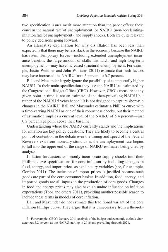
384 Brookings Papers on Economic Activity, Spring 2011
two specification issues merit more attention than the paper offers: these concern the natural rate of unemployment, or NAIRU (non-accelerating-inflation rate of unemployment), and supply shocks. Both are quite relevant to policy decisions going forward.
An alternative explanation for why disinflation has been less than expected is that there may be less slack in the economy because the NAIRU has risen. Temporary forces—including extended unemployment insur-ance benefits, the large amount of skills mismatch, and high long-term unemployment—may have increased structural unemployment. For exam-ple, Justin Weidner and John Williams (2011) estimate that such factors may have increased the NAIRU from 5 percent to 6.7 percent.
Ball and Mazumder largely ignore the possibility of a temporarily higher NAIRU. In their main specification they use the NAIRU as estimated by the Congressional Budget Office (CBO). However, CBO’s measure at any given point in time is not an estimate of the then-prevailing NAIRU but rather of the NAIRU 5 years hence.3 It is not designed to capture short-run changes in the NAIRU. Ball and Mazumder estimate a Phillips curve with a time-varying NAIRU as one of their robustness checks, but their method of estimation implies a current level of the NAIRU of 5.4 percent—just 0.2 percentage point above their baseline.
Understanding where the NAIRU currently stands and the implications for inflation are key policy questions. They are likely to become a central point of contention in the debate over the timing and speed of the Federal Reserve’s exit from monetary stimulus as the unemployment rate begins to fall into the upper end of the range of NAIRU estimates being cited by analysts.
Inflation forecasters commonly incorporate supply shocks into their Phillips curve specifications for core inflation by including changes in food, energy, and import prices as explanatory variables (see, for example, Gordon 2011). The inclusion of import prices is justified because such goods are part of the core consumer basket. In addition, food, energy, and imported goods are all inputs in the production of core goods. Changes in food and energy prices may also have an undue influence on inflation expectations (Topa and others 2011), providing another possible reason to include these terms in models of core inflation.
Ball and Mazumder do not estimate this traditional variant of the core inflation Phillips curve. They argue that it is unnecessary from a theoreti-
3. For example, CBO’s January 2011 analysis of the budget and economic outlook char-acterizes 5.2 percent as the NAIRU starting in 2016 and prevailing through 2021.

COMMENTS and DISCUSSION 385
cal point of view, and they cite previous work suggesting that these terms have become less important over time with increased Federal Reserve vigilance with respect to supply shocks. Nevertheless, the omission seems like a shortcoming on two grounds. First, the world continues to change over time in ways that bear on the influence of these factors on inflation in the United States. Although food and energy costs have become a smaller share of total U.S. production costs over the years, import prices should have become a much bigger deal as the economy has become ever more open. Such changes caution against using older studies to gauge whether to include these terms when estimating the Phillips curve. Second, prices of these goods have accelerated of late, quite notably in the case of energy. These trends, together with the risk that continued brisk growth in emerg-ing economies will drive up energy prices further, imply that now might be a particularly bad time for policymakers to ignore how these variables may influence inflation.
Finally, turning to the “level anchoring” of inflation expectations, Ball and Mazumder provide interesting evidence suggesting that core infla-tion expectations have been largely (although not completely) anchored at 2.5 percent per year in recent years. It follows that such anchoring partly explains why inflation has not fallen more, given the extremely high degree of unused resources in the economy. This partial anchoring of inflation expectations (together with the acceleration in energy costs) may well be a reason to be optimistic that deflation will be avoided even if slack remains high. One might point to the experience of Japan in the early 2000s as further support for this view. Inflation in Japan fell into negative territory on the heels of that economy’s lost decade, but it bottomed out and stayed at a much higher value than a standard Phillips curve model would have predicted (Fuhrer, Olivei, and Tootell 2010). A key reason why inflation in Japan did not sink further appears to be that inflation expectations remained positive (for the most part) throughout the period.
That said, I second Ball and Mazumder’s caution that past performance does not guarantee future results. The evidence in the paper supports the notion that inflation expectations have been largely anchored in the recent past, but it is at best suggestive about what the future holds. There remains much to understand about how inflation expectations are formed. One cannot rule out the possibility of inflation expectations moving materially lower should the economy remain weak. Indeed, as my figure 1 shows, some hints of this happening appeared in the spring and summer of 2010, when inflation expectations implied by yields on Treasury inflation-protected securities sank and stayed low for several months in the face of what
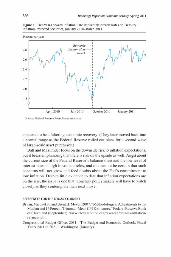
386 Brookings Papers on Economic Activity, Spring 2011
appeared to be a faltering economic recovery. (They later moved back into a normal range as the Federal Reserve rolled out plans for a second wave of large-scale asset purchases.)
Ball and Mazumder focus on the downside risk to inflation expectations, but it bears emphasizing that there is risk on the upside as well. Angst about the current size of the Federal Reserve’s balance sheet and the low level of interest rates is high in some circles, and one cannot be certain that such concerns will not grow and feed doubts about the Fed’s commitment to low inflation. Despite little evidence to date that inflation expectations are on the rise, the issue is one that monetary policymakers will have to watch closely as they contemplate their next move.
REfERENCES fOR ThE DyNaN COMMENT
Bryan, Michael F., and Brent H. Meyer. 2007. “Methodological Adjustments to the Median and 16 Percent Trimmed-Mean CPI Estimators.” Federal Reserve Bank of Cleveland (September). www.clevelandfed.org/research/data/us-inflation/ revmcpi.cfm.
Congressional Budget Office. 2011. “The Budget and Economic Outlook: Fiscal Years 2011 to 2021.” Washington (January).
Source: Federal Reserve Board/Haver Analytics.
Percent per year
1.8
2.0
2.2
2.4
2.6
2.8
April 2010 July 2010 October 2010 January 2011
BernankeJackson Hole
speech
Figure 1. five-year-forward Inflation Rate Implied by Interest Rates on Treasury Inflation-Protected Securities, January 2010–March 2011
COMMENTS and DISCUSSION 387
Fuhrer, Jeff, Giovanni Olivei, and Geoffrey M. B. Tootell. Forthcoming. “Inflation Dynamics When Inflation Is Near Zero.” Journal of Money, Credit and Banking.
Gordon, Robert J. 2011. “The History of the Phillips Curve: Consensus and Bifurca-tion.” Economica 78, issue 309: 10–50.
Topa, Giorgio, Wilbert van der Klaauw, Olivier Armantier, and Basit Zafar. 2011. “What Is Driving the Recent Rise in Consumer Inflation Expectations?” Liberty Street Economics (weblog), Federal Reserve Bank of New York (April 18). libertystreeteconomics.newyorkfed.org/.
Weidner, Justin, and John C. Williams. 2011. “What Is the New Normal Unemploy-ment Rate?” FRBSF Economic Letter 2011-05. Federal Reserve Bank of San Francisco (February 14).
Comment ByJAmeS H. StoCK1 It is tempting, particularly in monetary policy circles, to view the relatively modest fall in the rate of inflation during the Great Recession and its aftermath as a successful payoff for hard-won Federal Reserve credibility, which has anchored expectations around a credible implicit long-term target for inflation. It is therefore most welcome to have Laurence Ball and Sandeep Mazumder pit this hypothesis against others in their attempt to solve this “case of the missing disinflation.”
Ball and Mazumder’s explanation for the missing disinflation has two parts. First, less disinflation is missing than one might initially think: one just needs to measure inflation with median CPI inflation, which has fallen by more than core CPI inflation. Second, the Phillips curve has flattened since the mid-1980s, and the 1985–2007 backward-looking Phillips curve, applied to median CPI inflation, continues to fit after 2007. The authors argue that these two explanations account for the behavior of inflation from the Great Recession through 2010Q4, that a Gordon (1990)-type backward-looking accelerationist Phillips curve is stable over the 1985–2010 period, and that no further appeal to anchored expectations is needed; in short, there is no puzzle. Although the authors do find some evidence in the data of level anchoring, level-anchored expectations are not needed to understand inflation dynamics to date.
My comments consist of five points.First, Ball and Mazumder are correct to point out that the decline in
inflation observed during and since the recent recession is consistent with
1. I thank Mikkel Plagborg-Moller for research assistance in preparing this discussion. This work was supported in part by NSF Grant SES-0617811.
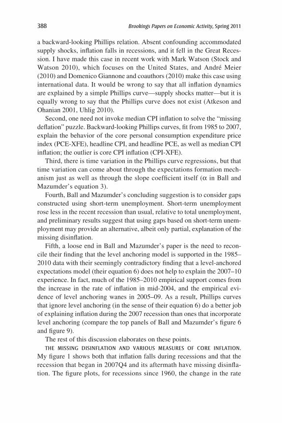
388 Brookings Papers on Economic Activity, Spring 2011
a backward-looking Phillips relation. Absent confounding accommodated supply shocks, inflation falls in recessions, and it fell in the Great Reces-sion. I have made this case in recent work with Mark Watson (Stock and Watson 2010), which focuses on the United States, and André Meier (2010) and Domenico Giannone and coauthors (2010) make this case using international data. It would be wrong to say that all inflation dynamics are explained by a simple Phillips curve—supply shocks matter—but it is equally wrong to say that the Phillips curve does not exist (Atkeson and Ohanian 2001, Uhlig 2010).
Second, one need not invoke median CPI inflation to solve the “missing deflation” puzzle. Backward-looking Phillips curves, fit from 1985 to 2007, explain the behavior of the core personal consumption expenditure price index (PCE-XFE), headline CPI, and headline PCE, as well as median CPI inflation; the outlier is core CPI inflation (CPI-XFE).
Third, there is time variation in the Phillips curve regressions, but that time variation can come about through the expectations formation mech-anism just as well as through the slope coefficient itself (a in Ball and Mazumder’s equation 3).
Fourth, Ball and Mazumder’s concluding suggestion is to consider gaps constructed using short-term unemployment. Short-term unemployment rose less in the recent recession than usual, relative to total unemployment, and preliminary results suggest that using gaps based on short-term unem-ployment may provide an alternative, albeit only partial, explanation of the missing disinflation.
Fifth, a loose end in Ball and Mazumder’s paper is the need to recon-cile their finding that the level anchoring model is supported in the 1985–2010 data with their seemingly contradictory finding that a level-anchored expectations model (their equation 6) does not help to explain the 2007–10 experience. In fact, much of the 1985–2010 empirical support comes from the increase in the rate of inflation in mid-2004, and the empirical evi-dence of level anchoring wanes in 2005–09. As a result, Phillips curves that ignore level anchoring (in the sense of their equation 6) do a better job of explaining inflation during the 2007 recession than ones that incorporate level anchoring (compare the top panels of Ball and Mazumder’s figure 6 and figure 9).
The rest of this discussion elaborates on these points.ThE MISSINg DISINflaTION aND vaRIOUS MEaSURES Of CORE INflaTION.
My figure 1 shows both that inflation falls during recessions and that the recession that began in 2007Q4 and its aftermath have missing disinfla-tion. The figure plots, for recessions since 1960, the change in the rate

COMMENTS and DISCUSSION 389
Figure 1. The “Williams Puzzle”a
Source: Author’s calculations.a. Each labeled point represents the change in 4-quarter inflation and unemployment from the indicated
quarter (a cyclical peak as identified by the Business Cycle Dating Committee of the National Bureau of Economic Research) to 10 quarters later. The figure omits the supply-shock recession that began in 1973Q4 and combines the recessions that began in 1980Q3 and 1981Q3 because those 10-quarter periods overlap. The regression lines are constrained to pass through the origin and are estimated excluding the 2007Q4 recession.
b. Average quarterly rate over the most recent 4 quarters, π4t = (π
t + π
t–1 + π
t–2 + π
t–3)/4.
c. Total civilian unemployment rate.
Change in inflation (percentage points)
Change in unemployment rate (percentage points)
Change in unemployment rate (percentage points)
Change in unemployment ratec (percentage points)1 2 3 4 5
Using median CPI inflation
Change in inflationb (percentage points)Using CPI-XFE inflation
Change in inflation (percentage points)Using PCE-XFE inflation
1960Q2
1969Q4
1980Q1
1990Q3
2001Q1 2007Q4
1 2 3 4 5
–4
–5
–6
–2
–3
–1
–2
–3
–1
–4
–5
–6
–2
–3
–1
1 2 3 4 5
1969Q4
1980Q1
1990Q3
2001Q1
2007Q4
1960Q2
1969Q41980Q11990Q3
2001Q12007Q4
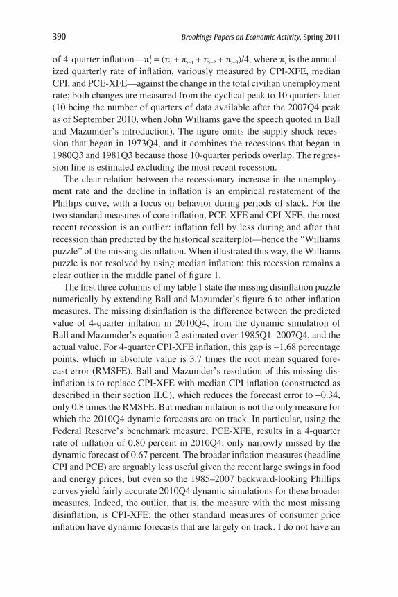
390 Brookings Papers on Economic Activity, Spring 2011
of 4-quarter inflation—p4t = (pt + pt-1 + pt-2 + pt-3)/4, where pt is the annual-
ized quarterly rate of inflation, variously measured by CPI-XFE, median CPI, and PCE-XFE—against the change in the total civilian unemployment rate; both changes are measured from the cyclical peak to 10 quarters later (10 being the number of quarters of data available after the 2007Q4 peak as of September 2010, when John Williams gave the speech quoted in Ball and Mazumder’s introduction). The figure omits the supply-shock reces-sion that began in 1973Q4, and it combines the recessions that began in 1980Q3 and 1981Q3 because those 10-quarter periods overlap. The regres-sion line is estimated excluding the most recent recession.
The clear relation between the recessionary increase in the unemploy-ment rate and the decline in inflation is an empirical restatement of the Phillips curve, with a focus on behavior during periods of slack. For the two standard measures of core inflation, PCE-XFE and CPI-XFE, the most recent recession is an outlier: inflation fell by less during and after that recession than predicted by the historical scatterplot—hence the “Williams puzzle” of the missing disinflation. When illustrated this way, the Williams puzzle is not resolved by using median inflation: this recession remains a clear outlier in the middle panel of figure 1.
The first three columns of my table 1 state the missing disinflation puzzle numerically by extending Ball and Mazumder’s figure 6 to other inflation measures. The missing disinflation is the difference between the predicted value of 4-quarter inflation in 2010Q4, from the dynamic simulation of Ball and Mazumder’s equation 2 estimated over 1985Q1–2007Q4, and the actual value. For 4-quarter CPI-XFE inflation, this gap is -1.68 percentage points, which in absolute value is 3.7 times the root mean squared fore-cast error (RMSFE). Ball and Mazumder’s resolution of this missing dis-inflation is to replace CPI-XFE with median CPI inflation (constructed as described in their section II.C), which reduces the forecast error to -0.34, only 0.8 times the RMSFE. But median inflation is not the only measure for which the 2010Q4 dynamic forecasts are on track. In particular, using the Federal Reserve’s benchmark measure, PCE-XFE, results in a 4-quarter rate of inflation of 0.80 percent in 2010Q4, only narrowly missed by the dynamic forecast of 0.67 percent. The broader inflation measures (headline CPI and PCE) are arguably less useful given the recent large swings in food and energy prices, but even so the 1985–2007 backward-looking Phillips curves yield fairly accurate 2010Q4 dynamic simulations for these broader measures. Indeed, the outlier, that is, the measure with the most missing disinflation, is CPI-XFE; the other standard measures of consumer price inflation have dynamic forecasts that are largely on track. I do not have an
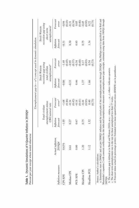
tabl
e 1.
Dyn
amic
Sim
ulat
ions
of 4
-Qua
rter
Infla
tion
in 2
010Q
4a
Perc
ent p
er y
ear
exce
pt w
here
not
ed o
ther
wis
e
U
nem
ploy
men
t gap
(u
- u*
) co
ncep
t use
d in
dyn
amic
sim
ulat
ion
Stoc
k-W
atso
n St
ock-
Wat
son
T
otal
civ
ilia
n re
cess
ion
gap
usin
g re
cess
ion
gap
usin
g
unem
ploy
men
t min
us
tota
l civ
ilia
n sh
ort-
term
C
BO
nat
ural
rat
e un
empl
oym
entb
unem
ploy
men
tc
A
ctua
l infl
atio
n,
Infla
tion
F
orec
ast
Infla
tion
F
orec
ast
Infla
tion
F
orec
ast
Infla
tion
mea
sure
20
10Q
4 fo
reca
st
erro
rd fo
reca
st
erro
r fo
reca
st
erro
r
CP
I-X
FE
0.
63%
-1
.05
-1.6
8 -0
.86
-1.4
9 -0
.31
-0.9
4
(0.4
6)
(0
.45)
(0.4
3)M
edia
n C
PI
0.61
0.
27
-0.3
4 -0
.33
-0.9
5 0.
30
-0.3
1
(0.4
2)
(0
.37)
(0.3
4)P
CE
-XF
E
0.80
0.
67
-0.1
4 0.
46
-0.3
4 0.
85
0.05
(0
.41)
(0.4
0)
(0
.40)
Hea
dlin
e C
PI
1.20
0.
75
-0.4
4 1.
37
0.17
0.
75
-0.4
5
(0.9
3)
(0
.93)
(0.9
2)H
eadl
ine
PC
E
1.12
1.
52
0.40
1.
66
0.54
1.
34
0.22
(0
.73)
(0.7
3)
(0
.73)
Sour
ce: A
utho
r’s
calc
ulat
ions
.a.
Sim
ulat
ions
sta
rt in
200
8Q1
and
use
pre-
2008
Q1
infla
tion
and
the
actu
al p
ath
of th
e un
empl
oym
ent r
ate
thro
ugh
2010
Q4.
The
Phi
llips
cur
ve is
spe
cifie
d as
in B
all a
nd
Maz
umde
r’s
equa
tion
2 w
ith c
onst
ant c
oeffi
cien
ts f
or t
he in
dica
ted
unem
ploy
men
t m
easu
res
and
unem
ploy
men
t ga
p co
ncep
ts, e
stim
ated
usi
ng d
ata
from
198
5Q1
thro
ugh
2007
Q4.
b. T
he r
eces
sion
gap
is d
efine
d as
in S
tock
and
Wat
son
(201
0), a
s u t
- m
in(u
t, u t
-1, .
. . ,
ut-
11),
whe
re t
indi
cate
s qu
arte
rs.
c. T
he s
hort
-ter
m u
nem
ploy
men
t rat
e is
the
rate
for
thos
e un
empl
oyed
less
than
27
wee
ks.
d. F
orec
ast m
inus
act
ual (
in p
erce
ntag
e po
ints
). E
stim
ated
roo
t mea
n sq
uare
d fo
reca
st e
rror
s (R
MSF
E)
are
in p
aren
thes
es.

392 Brookings Papers on Economic Activity, Spring 2011
explanation for why CPI-XFE is alone among these inflation measures in this regard. In any event, one need not appeal to median CPI to resolve the missing disinflation.
ExPECTaTIONS aNChORINg aND INflaTION DyNaMICS. Ball and Mazum-der’s Phillips curve has a time-varying slope (time-varying a in equation 3), which they interpret according to Ball, Gregory Mankiw, and David Romer’s (1988) implication that a increases in magnitude with the level and vari-ance of inflation. Because a varies over time, the cumulative effect of a sustained unit increase in the unemployment gap in a dynamic simulation varies over time, being greatest in the 1970s (when a is estimated to be greatest) and less in the 1960s and the 2000s. Here I will show by example that this time-varying cumulative effect can be achieved without invoking a time-varying a; instead, one can rely solely on time variation in how inflation expectations are formed. The less expectations drift, the smaller is the cumulative dynamic response to a unit increase in the gap.
I illustrate this point using the Phillips curve specification of Stock and Watson (2010), modified to include a contemporaneous activity term as in Ball and Mazumder’s paper. Rewrite their equation 1 as pt = pe
t + axt + et, where xt is the activity gap. In Ball and Mazumder’s equation 3, pe
t = p4t-1,
where p4t is the 4-quarter rate of inflation, p4
t = (pt + pt-1 + pt-2 + pt-3)/4.2 In the Stock and Watson (2010) model, pe
t is the filtered estimate of trend inflation obtained from a univariate model with unobserved permanent and transitory components, in which the variances of the two components fol-low random walks in logarithms. This unobserved components–stochastic volatility (UC-SV) model implies that Dpt is approximately a first-order moving-average process with a time-varying coefficient qt, where qt is large when the variance of the permanent component of inflation is small relative to the variance of the transitory component. As shown in Stock and Watson (2010), this model implies that pe
t ≈ (1 - qt) S i∞
= 0q itpt-1-i,
where the approximation holds when qt varies slowly. In the model, time variation enters through the coefficients on lagged inflation, not through the slope coefficient a. This time variation derives directly from variation in the fraction of the variance of the change in inflation due to permanent movements in inflation.
Time variation in the coefficients on lagged inflation, combined with a stable value of a, has three implications. First, it implies time variation in the response of inflation to a given path of unemployment in a dynamic
2. Ball and Mazumder’s expected inflation forecast is the same as Atkeson and Ohanian’s (2001).

COMMENTS and DISCUSSION 393
simulation. In particular, consider a dynamic simulation in which the out-put gap is hypothetically increased by 1 unit for k periods. In the UC-SV model, the change in inflation after k periods arising from this hypotheti-cal gap increase is a[1 - qt(k - 1)/k], which, for large k, is approximately a(1 - qt). The larger is qt, the less inflation falls in the long run. Large values of qt arise when most of the movements of inflation are transitory. In the post-1960 data, this was the case in the 1960s and after 1990. These episodes of mainly transitory changes in inflation can be interpreted as peri-ods of expectations anchoring, which arose because of the recent behavior of inflation (the Federal Reserve’s deeds, not its words). This anchoring produces a flatter dynamic response to a given increase in the gap. Sec-ond, if the data used in the regressions are temporally aggregated relative to the time horizon at which a is constant (the time horizon relevant for price-setting decisions), then time variation in the inflation lag coefficients will induce time variation in the population value of a in the temporally aggregated regression. Under plausible assumptions (for example, that the first autocovariances of xt are positive), larger values of qt induce smaller time-aggregated values of a. Third, by a standard omitted-variables argu-ment, ignoring this time variation in the coefficients on lagged inflation can induce apparent time variation in a.
My table 2 examines the third of these implications by reporting esti-mates of a using two alternative measures of pe
t: pet = p4
t-1 as in Ball and Mazumder’s equation 3, and pe
t measured as t - 1 dated filtered trend infla-tion from the Stock and Watson (2007) UC-SV model, as in Stock and Watson (2010). The slope coefficient is estimated for three subsamples: 1960–72, 1973–84, and 1985–2010. The top panel reports results where the unemployment gap is measured using the CBO natural rate of un-employment series, as in the Ball and Mazumder paper. Consistent with their findings, stability of a is rejected at the 5 percent level for CPI-XFE when their measure of pe
t is used (first four columns); although it is rejected at only the 10 percent level for median CPI and PCE-XFE, the change in estimated coefficients across subsamples is economically large. In contrast, the magnitude of the instability is reduced and the hypothesis of stability is not rejected at the 10 percent level (p values > 0.25) for both CPI-XFE and PCE-XFE when the UC-SV measure of pe
t is used (final four columns). Stability is rejected for the median CPI, but perhaps this is related to dif-ferences in the construction of the original and revised series, which were spliced together to create the full time series. The gap using the CBO natu-ral rate series is problematic because it is two-sided, so the middle panel provides results for the Stock and Watson (2010) recession gap, in which

tabl
e 2.
Sta
bilit
y of
Phi
llips
Cur
ve S
lope
Coe
ffici
ents
, 196
0–20
10a
Perc
ent p
er y
earb
E
xpec
ted
infla
tion
pe t i
s m
easu
red
as in
Bal
l and
Maz
umde
rc E
xpec
ted
infla
tion
pe t i
s m
easu
red
usin
g U
C-S
V m
odel
d
Infla
tion
mea
sure
19
60–7
2 19
73–8
4 19
85–2
010
Cho
w p
e 19
60–7
2 19
73–8
4 19
85–2
010
Cho
w p
Une
mpl
oym
ent g
ap is
tota
l civ
ilia
n un
empl
oym
ent r
ate
min
us C
BO
nat
ural
rat
eC
PI-
XF
E
-0.2
3 -0
.67
-0.1
3 0.
035
-0.1
3 -0
.37
-0.1
2 0.
285
(0
.07)
(0
.21)
(0
.04)
(0.0
5)
(0.1
6)
(0.0
2)M
edia
n C
PIf
-0.2
6 -0
.64
-0.1
6 0.
033
0.02
-0
.59
-0.1
9 0.
000
(0
.04)
(0
.21)
(0
.05)
(0.0
4)
(0.1
9)
(0.0
5)P
CE
-XF
E
-0.1
7 -0
.42
-0.1
0 0.
090
-0.0
8 -0
.24
-0.1
1 0.
273
(0
.07)
(0
.15)
(0
.04)
(0.0
4)
(0.0
9)
(0.0
2)U
nem
ploy
men
t gap
is S
tock
-Wat
son
rece
ssio
n ga
pg usi
ng to
tal c
ivil
ian
unem
ploy
men
t rat
eC
PI-
XF
E
-0.2
9 -0
.50
-0.1
1 0.
003
-0.1
7 -0
.29
-0.1
0 0.
083
(0
.11)
(0
.12)
(0
.03)
(0.0
6)
(0.0
9)
(0.0
2)M
edia
n C
PIf
-0.3
0 -0
.50
-0.1
5 0.
005
-0.2
2 -0
.48
-0.1
2 0.
006
(0
.07)
(0
.11)
(0
.04)
(0.1
3)
(0.0
9)
(0.0
6)P
CE
-XF
E
-0.1
7 -0
.26
-0.0
9 0.
069
-0.1
0 -0
.15
-0.1
0 0.
607
(0
.08)
(0
.07)
(0
.03)
(0.0
5)
(0.0
5)
(0.0
2)

Une
mpl
oym
ent g
ap is
Sto
ck-W
atso
n re
cess
ion
gap
usin
g sh
ort-
term
une
mpl
oym
ent r
ate
CP
I-X
FE
-0
.34
-0.7
3 -0
.23
0.03
6 -0
.20
-0.4
8 -0
.20
0.11
3
(0.1
4)
(0.1
8)
(0.0
6)
(0
.07)
(0
.13)
(0
.04)
Med
ian
CP
If -0
.36
-0.7
3 -0
.33
0.06
8 -0
.28
-0.7
3 -0
.22
0.02
0
(0.0
8)
(0.1
7)
(0.0
4)
(0
.15)
(0
.14)
(0
.14)
PC
E-X
FE
-0
.19
-0.3
6 -0
.17
0.30
9 -0
.11
-0.2
2 -0
.17
0.43
9
(0.1
1)
(0.1
0)
(0.0
7)
(0
.06)
(0
.07)
(0
.05)
Sour
ce: A
utho
r’s
calc
ulat
ions
.a.
The
Phi
llips
cur
ve s
lope
a is
est
imat
ed u
sing
the
follo
win
g eq
uatio
n: p
t = p
e t + a
(u -
u*)
t + e
t. A
ll es
timat
es u
se q
uart
erly
dat
a fr
om 1
960Q
1 th
roug
h 20
10Q
4 ex
cept
as
note
d ot
herw
ise.
New
ey-W
est s
tand
ard
erro
rs w
ith e
ight
lags
are
in p
aren
thes
es.
b. A
nnua
lized
cha
nge
in th
e lo
gari
thm
of
the
pric
e le
vel.
c. M
easu
red
as th
e av
erag
e of
qua
rter
ly r
ates
of
infla
tion
over
the
prev
ious
fou
r qu
arte
rs: p
e t = p
4 t-1 =
(p t
-1 +
pt-
2 + p
t-3 +
pt-
4)/4
. Est
imat
es m
ay n
ot m
atch
thos
e in
Bal
l and
M
azum
der,
this
vol
ume,
bec
ause
of
min
or d
iffe
renc
es in
dat
a vi
ntag
es a
nd tr
ansf
orm
atio
ns. S
ee th
e au
thor
’s w
ebsi
te f
or f
urth
er d
etai
ls.
d. M
easu
red
usin
g th
e un
obse
rved
com
pone
nts–
stoc
hast
ic v
olat
ility
mod
el o
f St
ock
and
Wat
son
(200
7); s
ee te
xt.
e. p
val
ues
for
the
Cho
w te
st o
f eq
ualit
y of
the
coef
ficie
nts
estim
ated
for
the
thre
e su
bsam
ples
for
the
indi
cate
d in
flatio
n an
d un
empl
oym
ent g
ap c
ombi
natio
n.f.
Con
stru
cted
by
splic
ing
the
orig
inal
and
rev
ised
ser
ies
of t
he F
eder
al R
eser
ve B
ank
of C
leve
land
at
Janu
ary
1983
and
cal
cula
ting
quar
terl
y an
nual
ized
gro
wth
rat
es
as d
escr
ibed
in B
all a
nd M
azum
der,
this
vol
ume,
sec
tion
II.C
. Est
imat
es in
the
first
col
umn
are
base
d on
dat
a fo
r 19
67Q
2–19
72Q
4 be
caus
e ea
rlie
r da
ta a
re n
ot a
vaila
ble.
g. D
efine
d as
in S
tock
and
Wat
son
(201
0) a
s u t
- m
in(u
t, u t
-1, .
. . ,
ut-
11),
whe
re t
indi
cate
s qu
arte
rs.

396 Brookings Papers on Economic Activity, Spring 2011
the natural rate is the minimum value of the unemployment rate over the current and past 11 quarters. The stability results are broadly similar to those for the CBO gap.3
ThE NaTURal RaTE, gaPS, aND ShORT-TERM UNEMPlOyMENT. A different explanation of the missing disinflation is that the unemployment gap is mismeasured. Movements in the natural rate of unemployment (and in potential GDP) are quite difficult to measure, even with the benefit of many years of hindsight (see, for example, Staiger, Stock, and Watson 1997, Orphanides 2001). Compared with previous recessions, one unfortunate feature of the recent recession and its aftermath is that long-term unem-ployment is an unusually large fraction of total unemployment. The paper in this volume by Alan Krueger and Andreas Mueller shows that job search intensity (measured as hours per week spent in job search) declines with the duration of unemployment. If the intensity of job search, particularly among those with recent job experience and thus fresh job skills, is what matters for downward wage pressure, then short-term unemployment might provide a better measure of the natural rate than total unemployment.4
As figure 2 shows, the short-term unemployment rate rose by less than usual during the recent recession, given the increase in total unemployment. Indeed, when figure 1 is recomputed using the short-term unemployment rate, as is done in my figure 3, the “Williams puzzle” disappears entirely. Although this complete disappearance is sensitive to the 10-quarter hori-zon, figures 2 and 3 suggest that focusing on short-term unemployment, combined with time-varying expectation formation as discussed above, could further stabilize the Phillips relations.
Evidence on this conjecture is reported in the final two columns of table 1 and in the bottom panel of table 2. The estimate in table 1 of the missing disinflation for CPI-XFE of 1.68 percentage points is reduced to 0.94 percentage point (2.2 times the RMSFE) when the short-term unem-ployment recession gap is used. When short-term unemployment is used, there is virtually no missing disinflation if inflation is measured using PCE-XFE. Moreover, the coefficients in the PCE-XFE Phillips curve using
3. These findings are also robust to using a natural rate computed as a one-sided expo-nential filter of the unemployment rate. This analysis does not address temporal aggregation. If the time scale for price setting decisions is shorter than a quarter, then because of time aggregation one would still expect instability in a in the regressions in table 2 with UC-SV expectations, even if the UC-SV specification is correct. Exploring the effect of time aggre-gation is left for future work.
4. Earlier suggestions that the natural rate has risen during the slow recovery include Kocherlakota (2010) and Valletta and Kuang (2010).

COMMENTS and DISCUSSION 397
the short-term unemployment recession gap are stable over the three sub-samples in table 2, both statistically and economically, and the hypothesis that a is stable cannot be rejected for CPI-XFE when the UC-SV inflation expectation is used (table 2, bottom panel, final four columns).
ThE 2004 EPISODE.5 Inflation picked up sharply in the middle of 2004 despite the sluggish recovery: in 2004Q2, median CPI inflation rose more than 50 basis points even though the CBO unemployment gap was +0.6 percentage point. This increase in the rate of inflation was sustained, and the Federal Reserve put behind it fears of a further “unwelcome fall in inflation” (Bernanke 2003).
The 2004 episode, in particular the data for 2004Q2, plays an important role driving Ball and Mazumder’s empirical finding of support for level anchoring, especially the large values of the smoothed estimates of d in the late 2000s reported in the bottom two panels of their figure 8. These pre-sent the estimated path of dt from the Kalman smoother, which uses the full dataset. My figure 4 presents both the Kalman smoother estimate and the Kalman filter estimate (the filter uses only data through date t, whereas the
Source: Bureau of Labor Statistics.a. Rates are for all civilian workers.b. Unemployed less than 27 weeks.
Percent
Total
Short-termb
2
1
4
6
8
10
3
5
7
9
1960 1970 1980 1990 2000 2010
Figure 2. Total and Short-Term Unemployment Rates, 1952–2011Q1a
5. The ideas in this section stem from communications with Ball and Mazumder. For additional discussion of this episode, see Billi (2009).
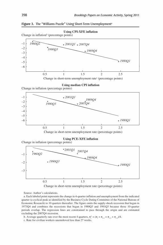
398 Brookings Papers on Economic Activity, Spring 2011
Source: Author’s calculations.a. Each labeled point represents the change in 4-quarter inflation and unemployment from the indicated
quarter (a cyclical peak as identified by the Business Cycle Dating Committee of the National Bureau of Economic Research) to 10 quarters thereafter. The figure omits the supply-shock recession that began in 1973Q4 and combines the recessions that began in 1980Q3 and 1981Q3 because those 10-quarter periods overlap. The regression lines are constrained to pass through the origin and are estimated excluding the 2007Q4 recession.
b. Average quarterly rate over the most recent 4 quarters, π4t = (π
t + π
t–1 + π
t–2 + π
t–3)/4.
c. Rate for civilian workers unemployed less than 27 weeks.
Change in inflation (percentage points)
Change in short-term unemployment rate (percentage points)
Change in short-term unemployment rate (percentage points)
Change in short-term unemployment ratec (percentage points)0.5 1 1.5 2 2.5
Using median CPI inflation
Change in inflationb (percentage points)Using CPI-XFE inflation
Change in inflation (percentage points)Using PCE-XFE inflation
0.5 1 1.5 2 2.5
–4
–5
–6
–2
–3
–1
–2
–3
–1
–4
–5
–6
–2
–3
–1
0.5 1 1.5 2 2.5
1960Q2
1969Q4
1980Q1
1990Q3
2001Q1 2007Q4
1969Q4
1980Q1
1990Q3
2001Q1
2007Q4
1960Q21969Q4
1980Q11990Q3
2001Q1 2007Q4
Figure 3. The “Williams Puzzle” Using Short-Term Unemploymenta
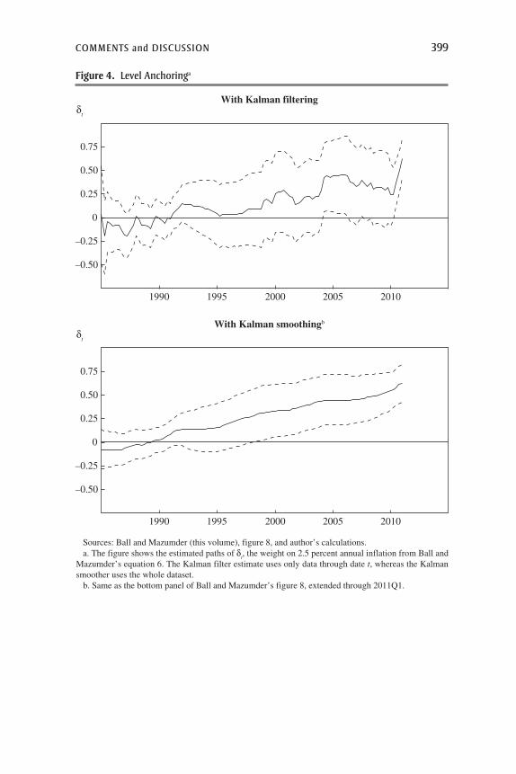
COMMENTS and DISCUSSION 399
Sources: Ball and Mazumder (this volume), figure 8, and author’s calculations.a. The figure shows the estimated paths of δ
t, the weight on 2.5 percent annual inflation from Ball and
Mazumder’s equation 6. The Kalman filter estimate uses only data through date t, whereas the Kalman smoother uses the whole dataset.
b. Same as the bottom panel of Ball and Mazumder’s figure 8, extended through 2011Q1.
δt
With Kalman filtering
1990 1995 2000 2005 2010
δt
With Kalman smoothingb
–0.50
–0.25
0
0.50
0.25
0.75
1990 1995 2000 2005 2010
–0.50
–0.25
0
0.50
0.25
0.75
Figure 4. level anchoringa

400 Brookings Papers on Economic Activity, Spring 2011
smoother uses the full dataset, that is, is two-sided). Figure 4 also extends the dataset to 2011Q1. Influential observations can be identified by jumps in the filtered estimate of dt. A large jump is evident in 2004Q2, indicating that much of the support in the 2000s for level anchoring arises from this observation.6 Split-sample regressions reinforce this conclusion. When a constant-coefficient version of Ball and Mazumder’s equation 6 is esti-mated for the 5 years 2000Q1–2004Q4, the estimated value of d is 0.53; for the subsequent 5 years the estimated value of d falls to 0.25. Evidently, the support for level anchoring is heavily influenced by 2004; from 2005 to 2009, the empirical support for level anchoring diminishes relative to the first half of the decade, so that Phillips curves that ignore level anchoring do better at explaining the 2007–09 period.
CONClUSION. Ball and Mazumder have written a stimulating and creative paper on a centrally important topic. In my view, they are right on many counts: during the recent recession and its aftermath, inflation has fallen by less than one might initially have expected; notwithstanding this appar-ent missing disinflation, a clear Phillips relation is evident in these data; and incorporating a modest amount of time variation explains this missing disinflation. It might be that the data are too limited to allow one to ascer-tain whether this time variation arises through a time-varying expectations formation process or through a direct change in the slope coefficient a. Pre-liminary results presented in this discussion support Ball and Mazumder’s concluding suggestion that the gap might be better measured using short-term unemployment, and more work on this question is warranted. None of these explanations invoke strict level anchoring of expectations.
The real test for the level anchoring theory is just around the corner. Cur-rently, all the unemployment gaps considered here remain positive, with 2011Q1 estimates ranging from +0.6 percentage point for the short-term unemployment rate recession gap to +3.7 percentage points for the CBO unemployment gap. Depending on the gap used, an accelerationist Phillips curve would predict inflation to stabilize at a low rate or to decline further. In contrast, if expectations are anchored at, say, 2 percent, and if these expectations influence price setting, then inflation should begin to climb back to its long-term target value. Recent data hint that such a return to
6. Sbordone and others (2010) reach a similar conclusion about mid-2004 using an approach that seems different from but is actually quite closely related to the simpler approach here. In the context of their model, they interpret mid-2004 as evidence of an increase in the public’s perception of the Federal Reserve’s inflation target and that, through expectations management, the Fed was able to avoid a slide into deflation.

COMMENTS and DISCUSSION 401
target is under way; indeed, the final two observations using the Kalman filter in figure 4, for 2010Q4 and 2011Q1, show the sharpest increase yet in the filtered estimate of Ball and Mazumder’s dt. These most recent data are confounded by sharp energy and food price increases, which might be par-tially passed through to core inflation, and it is too early to know whether this uptick in inflation is permanent. But there was a return from very low inflation in 2004 despite positive gaps. Whether there will be a second such return will be a test of the expectations anchoring theory in a way that the decline of inflation so far during this episode is not.
REfERENCES fOR ThE STOCk COMMENT
Atkeson, Andrew, and Lee E. Ohanian. 2001. “Are Phillips Curves Useful for Forecasting Inflation?” Federal Reserve Bank of Minneapolis Quarterly Review 25, no. 1: 2–11.
Bernanke, Ben S. 2003. “An Unwelcome Fall in Inflation?” Speech before the Economics Roundtable, University of California, San Diego, July 23. www.federalreserve.gov/boarddocs/speeches/2003/20030723/.
Billi, Roberto M. 2009. “Was Monetary Policy Optimal during Past Deflation Scares?” Federal Reserve Bank of Kansas City Economic Review (3rd Quarter): 67–98.
Giannone, Domenico, Michele Lenza, Daphne Momferatou, and Luca Onorante. 2010. “Short-Term Inflation Projections: A Bayesian Vector Autoregressive Approach.” Frankfurt: European Central Bank.
Gordon, Robert J. 1990. “U.S. Inflation, Labor’s Share, and the Natural Rate of Unemployment.” In Economics of Wage Determination, edited by Heinz Konig. Berlin: Springer-Verlag.
Kocherlakota, Naryana. 2010. “Inside the FOMC.” Speech at Northern Michigan University, Marquette, Mich., August 17. www.minneapolisfed.org/news_events/pres/speech_display.cfm?id=4525.
Meier, André. 2010. “Still Minding the Gap—Inflation Dynamics during Episodes of Persistent Large Output Gaps.” Working Paper no. WP/10/189. Washington: International Monetary Fund.
Orphanides, Athanasios. 2001. “Monetary Policy Rules Based on Real-Time Data.” American Economic Review 91: 964–85.
Sbordone, Argia M., Andrea Tambalotti, Krishna Rao, and Kieran Walsh. 2010. “Policy Analysis Using DSGE Models: An Introduction.” FRBNY Economic Policy Review (October): 23–43.
Staiger, Doug, James H. Stock, and Mark W. Watson. 1997. “How Precise Are Estimates of the Natural Rate of Unemployment?” In Reducing Inflation: Moti-vation and Strategy, edited by Christina Romer and David Romer. University of Chicago Press.
Stock, J. H., and M. W. Watson. 2007. “Why Has U.S. Inflation Become Harder to Forecast?” Journal of Money, Credit, and Banking 39: 3–34.
402 Brookings Papers on Economic Activity, Spring 2011
———. 2010. “Modeling Inflation after the Crisis.” In Macroeconomic Chal-lenges: The Decade Ahead. Proceedings of the Federal Reserve Bank of Kansas City 2010 Jackson Hole Symposium. Kansas City, Mo.: Federal Reserve Bank of Kansas City.
Uhlig, Harald. 2010. “Economics and Reality.” Working Paper no. 16416. Cam-bridge, Mass.: National Bureau of Economic Research.
Valletta, Rob, and Katherine Kuang. 2010. “Is Structural Unemployment on the Rise?” FRBSF Economic Letter no. 2010–34. Federal Reserve Bank of San Francisco (November 8).
GeneRAL DISCUSSIon George Perry agreed that a better under-standing of the historical Phillips curve and its recent behavior was needed. Although he appreciated the tractability of the authors’ model, he believed it had two important problems. One was that it ignored downward nominal wage rigidity, which moderates the effects of high unemployment on infla-tion and helps explain what is happening today. The other was that the model’s unitary elasticity between past and present inflation is not supported by the data except in the high-inflation period around the 1970s. At that time wage setting was dominated by union contracts indexed to inflation, the economy was buffeted by large inflationary shocks from several sources, and inflationary expectations were measurably rising. Because so much of the variance of inflation occurs in those years, they dominate regressions fitted over longer periods that include them. But it is misleading, Perry felt, to use the model to estimate high employment targets or inflation risks at other times, or to assess present developments.
Robert Gordon praised the paper’s basic methodology, which was to analyze the performance of equations based on dynamic simulations over a period that excludes the puzzle of the last three years. He went on to compare the paper’s results with those of his own triangle model, which had now been exposed to 30 years of additional data. That model differs from the authors’ and others both by including four explicit supply shocks—food and energy effects, relative import prices, productivity trend changes, and Nixon-era price control dummies—and by including longer lags on both the unemployment rate and inflation. As the top panel of the authors’ figure 1 showed, headline inflation followed a characteristic zigzag in 2008, 2009, and 2010, related to the collapse and then recovery of oil prices. The triangle model simulation mimics that movement and winds up almost exactly on target in 2010. It turned out, Gordon reported, that the key factor in generat-ing these results related to the anchoring of expectations. The unemployment gap pulls inflation down in the last two years, but the six years of lagged

COMMENTS and DISCUSSION 403
inflation terms make the initial process of disinflation very slow, as it is still influenced by 2004, 2005, and 2006. Further, Gordon argued, the erroneous impression that the Phillips curve slope has shifted was due to omitted variables, which have a systematic bias on the unemployment gap term. What has changed, he suggested, is that there has been a substantial reduc-tion in the impact of oil prices and food and energy prices on both core and headline inflation.
John Haltiwanger cited evidence of some fundamental structural changes in the economy over the last several decades that affected the Phillips curve relationship. There had been a striking declining trend in the inflow rate to unemployment, and increased volatility in business growth seemed to account for a reasonably large fraction of that decline. It was important, Haltiwanger argued, to understand what those structural changes were and their implications for price changes.
Alan Krueger noted a related phenomenon, namely, that in fitting wage Phillips curves, the expectation that emerges is for wages to be declining. Fitting Phillips curves by decile of the distribution suggests that the lower deciles are where the overprediction is occurring, and that certain segments of the labor market may not be exerting much pressure on wages.
Christopher Sims agreed that the Phillips curve was interesting and useful as a statistical relationship but questioned whether it should be the central focus of forecasting and policymaking with regard to inflation. Allowing the slope of the curve to change over time and including food and energy prices on the right-hand side are important approaches to “rescuing” the Phillips curve, but they do not rescue the idea of its central importance. Forecasting inflation and making policy about inflation require an under-standing of what is changing the NAIRU, food and energy prices, import prices, and so on, and how policies affect those things. That requires a model with more than one equation.
Martin Baily agreed with Krueger that it was important to take into account which groups of workers put more pressure on wages than others. The persistence of wage stickiness was also a puzzle, because in the last few recessions, and dramatically in the most recent one, the relationship between employers and employees has changed. The recent recession saw a massive drop in employment and a drop in the number of workers who are unionized. And even union wages have shown some downward flexibility of late.
Justin Wolfers argued that although the Phillips curve has not been proved false, that may be because it is not falsifiable. The fact that there are so many degrees of freedom to consider may be what has saved the
404 Brookings Papers on Economic Activity, Spring 2011
Phillips curve from falsification. Inflation can be measured either as headline, core, or median, using either the PCE deflator, the CPI, or the GDP deflator. Inflation expectations can be modeled as rational, adaptive, or anchored. Data from different surveys can be utilized, such as the Livingston, the SPF, the Blue Chip, and the Michigan survey. Different measures of slack can be used, from the unemployment rate to the output gap to capacity utilization. The long-term unemployed can be included or not. Coefficients can be fixed or allowed to change over time. The lag structure can be adjusted, and nonlinearities can be assumed or ignored. Regime shifts can be invoked. Supply shocks can be included, including shocks to food, energy, and import prices, and price controls can be a factor in certain periods. Some economists in addition want to control for productivity or the labor share. In the end, there are more degrees of freedom than there are observations, which means that whatever path inflation might take, some researcher could plausibly claim to have found a Phillips curve that accounts for that path.
James Stock responded that the basic fact remained that inflation in the United States and in other developed economies falls during periods of slack. This had happened during the 1960s recession and again during the 1969 recession. The 1973 recession was different because of the oil price shock, but the pattern reappeared in the early-1980s and 1990 recessions, and again in 2000 for a while, except for a very interesting episode in 2004 and 2005. And much the same thing happened in 2007 and after, although the scale of it was in question. The issue then was not whether the pattern exists, but how to model it. There were real reasons such as changes in monetary policy, for including things like time variation and regime shifts. The analysis was not simple, but there was a statistical regularity there to be studied.
Jeremy Nalewaik noted that the paper presented inflation forecasts that were below the latest median forecast from the Survey of Professional Forecasters for 2011 and 2012, and he wondered why that median forecast would be higher. He conjectured that it could have something to do with the forecasters in that survey placing more weight on hysteresis stories.
Benjamin Friedman thought it would be helpful to distinguish much more precisely between backward-looking expectations and inflation anchoring. This was not merely a question of semantics, he argued. It mattered because the notion of anchoring expectations, at least in the policy literature, normally conveys something about the ability of the central bank or other policy makers to influence expectations in more than just a backward-looking way. Absent that idea, it was not clear what anchoring means other than that people form their expectations by looking backward.

COMMENTS and DISCUSSION 405
William Brainard stated that a common rationale for excluding food and energy price changes from core inflation is that they frequently reflect tran-sitory shocks and are therefore less likely to lead to increases in prices of other goods or in wages than are price increases due to permanent shocks. Median inflation does not recognize this distinction. For example, price changes for computer chips have been persistent and large (and negative) but are in effect filtered out in the median estimate. It would be interesting to know whether the persistence of price increases in food and energy or in goods in general has changed in recent years, and whether weighting price changes by persistence improves forecasts of future inflation. Brainard also commented on inflation targeting, arguing that it was important to dis-tinguish the effect of the Federal Reserve announcing inflation targets on financial markets and the effect on the pricing behavior of firms that actually set the prices of goods and services. He argued that there is little reason for most such firms to be swayed by statements about targets two years in the future, and he reported that in interviews with over 500 nonfinancial firms, Truman Bewley had found that virtually none paid attention in their pricing decisions to statements by the Federal Reserve.