Inferring Treatment Status When Treatment Assignment is Unknown: Detecting Collusion in Timber Auctions*

John A. List, University of Chicago and NBER

Daniel L. Millimet

Southern Methodist University

Michael K. Price University of Nevada-Reno

February 2007

Abstract

Economists have struggled with the task of detecting collusion without a smoking gun. In this paper, we draw on the program evaluation literature to provide a new approach to detecting collusion. Rather than using data on treatment assignment and outcomes to evaluate effects, we use theory to put structure on expected effects, and show how to infer treatment status from outcomes alone. Our approach clarifies many issues in the collusion literature; it rejects the validity of some existing approaches and uncovers new approaches not previously considered. We apply our approach to examine bidder behavior in Canadian timber auctions. Our application is of special relevance in light of recent developments in the long-standing U.S.-Canadian softwood lumber dispute, in which the market price for federally-owned Canadian timber is to be determined using data on the winning bids from previously held auctions. Using data on nearly 3,000 auctions (over 10,000 individual bids) for cutting rights of standing timber in British Columbia from 1996-2000, we find mixed evidence of collusive behavior. KEYWORDS: Treatment effect, Collusion, Softwood lumber dispute JEL: C21, F18, Q23

* Numerous discussions with several Canadian officials, including, but not limited to, Bruce McRae, Michael Stone, and Bill Howard, considerably enhanced this paper. John Staub provided excellent research assistance. Leandra DiSilva and Christine Dobridge also provided excellent assistance during the data-gathering process. Larry Ausubel, Patrick Bajari, Peter Cramton, John Horowitz, Steve Levitt, Esfandiar Maasoumi, Michael Margolis, Tigran Melkonyan, Emily Oster, Jesse Shapiro, Chad Syverson, and Richard Woodward provided useful suggestions. The authors are also grateful to conference participants at the AEA Annual Conference, Chicago, IL, January 2007, and seminar participants at Iowa State U, U of Nevada – Reno, SMU, and Texas A&M. Corresponding author: Daniel L. Millimet, Department of Economics, Box 0496, SMU, Dallas, TX 75275-0496; email: millimet@mail.smu.edu; website: http://faculty.smu.edu/millimet/.

I. Introduction

The U.S.-Canada Softwood Lumber Dispute can be traced as far back as the 1820s with disputes between

New Brunswick and Maine. While trade restrictions on different lumber products have changed over time, the

legal issues underlying these restrictions have not. Extreme differences in resource ownership have led to

accusations by U.S. lumber producers that cutting rights for standing timber on Crown (public) lands are priced

below fair market value. The most recent dispute began in 2002, when the U.S. Coalition for Fair Lumber

Imports filed a countervailing duty (CVD) and an anti-dumping (AD) petition against Canadian softwood lumber.

Since then, negotiators have discussed various measures to lift the CVD/AD on a province-by-province case.

The proposed resolution with British Columbia – the largest player on the Canadian side – centers around

the implementation of a market based system for pricing cutting rights on public lands. Under this system, cutting

rights for standing timber on a portion of available public lands would be sold via a first-price, sealed-bid auction

to estimate a simple hedonic price function to determine the shadow values of a plot’s characteristics. These

shadow values would then be used to price cutting rights on non-auctioned lands. A necessary condition

articulated in this agreement is that the method provides a viable and robust signal for pricing public lands.

However, anecdotal evidence of collusive behavior by bidders in existing Canadian timber auctions abounds. As

a result, the agreement between the two countries threatens to become derailed unless it can be shown that

collusion does not undermine the integrity of the proposed pricing system.

Unfortunately, economists have long struggled with the task of detecting collusion in the absence of a

‘smoking gun’. Much of the previous collusion literature relies on case studies of specific markets, using court

records or internal firm documents to identify anti-competitive behavior. In this paper, we draw on the program

evaluation literature to provide a new approach to detecting collusion. Previous research related to our

application – detection of collusion – has proceeded in a literature distinct from the treatment effects literature

(see, e.g., Porter and Zona 1993, 1999; Baldwin et al. 1997; Pesendorfer 2000; Bajari and Ye 2003). Our

approach clarifies many issues of importance in the collusion literature; it rejects the validity of some common

approaches, and brings to light other approaches not previously considered.

Throughout the analysis, we view the problem of detecting collusion as analogous to one of identifying

treatment assignment given data on outcomes (in our case, auction bids). Since identifying treatment assignment

requires additional information beyond data on observed outcomes, we rely on insights from economic theory to

sign the expected treatment effect. Fortunately, the theoretical literature on bidding behavior in first-price

auctions is well developed, making transparent the conditions required for identification.

Applying our methodology, we assess whether the Canadian timber auctions that will be used to facilitate

a market pricing system were likely free of collusion. Making use of a unique data set that includes nearly 3,000

auctions (over 10,000 individual bids) for cutting rights of standing timber in British Columbia from 1996 – 2000,

we find mixed statistical evidence concerning whether, and to what extent, bidders engage in collusive behavior.

From a policy perspective this finding merits serious consideration; in a normative sense, this application raises

several issues that scholars should find useful.

While we believe our framework for addressing the problem at hand to be innovative, it is related to

several other distinct literatures. First, and most closely related, Jacob and Levitt (2003) use data on test scores

(outcomes) to infer teacher cheating (treatment assignment) using data from Chicago public schools. Although

this application is completely analogous to ours, the authors’ methodology is less general and it relies on

particular patterns of test answers to infer impropriety. Second, our problem is related to the literature on corrupt

data, although in this literature there is at least a ‘corrupt’ measure of treatment assignment. For example, Kreider

and Pepper (2006) utilize a variety of assumptions concerning the nature of reporting errors to bound the actual

disability rate given data on self-reported disability status. Third, our approach is related to the estimation of

finite mixture models which posit that the marginal distribution of a variable in question represents a mixture of

several distinct underlying distributions with observations drawn from unobserved population sub-types (see e.g.,

Cameron and Trivedi, 2005). Finally, time series models aimed at identifying unobserved structural breaks are

also similar in spirit.

The remainder of the paper is organized as follows. Section 2 discusses the issue of collusion in

Canadian timber auctions, as well as the theoretical model of collusion in auctions. Section 3 presents our

framework in which to infer unobserved treatment assignment. Section 4 describes the data. Section 5 discusses

the results. Section 5 concludes.

II. Collusion in Canadian Softwood Timber Auctions

U.S.-Canada Softwood Lumber Dispute

The U.S.-Canada softwood lumber dispute dates back to at least the 1820s when disputes occurred

between New Brunswick and Maine. Since that time both the U.S. and Canada have repeatedly imposed and

dropped duties on softwood lumber. While tariff rates on different lumber products have changed over time, the

legal issues have not. The two main issues are (i) the downward pressure on U.S. lumber prices due to imports of

Canadian lumber, and (ii) the ownership structure of Canadian forests (94% are publicly owned, resulting in U.S.

accusations of public subsidies; specifically, cutting rights for standing timber on federal lands are priced below

fair market value).

During the past two decades, U.S. producers have repeatedly filed CVD petitions with the U.S.

International Trade Commission (ITC). The most recent dispute began in 2002 when the Coalition for Fair

Lumber Imports (CFLI) filed a CVD petition and an AD petition. In April 2002, the Department of Commerce

(DoC) released a final determination in the subsidy and antidumping case, setting a combined CVD/AD rate of

27.22%.1 Since the DoC's ruling, negotiators have discussed various measures to be undertaken on a province-by-

province basis to lift the CVD/AD.

The proposed solution with respect to British Columbia (BC) – the largest player in Canada – revolves

around a market-based system.2 Under the proposal, cutting rights on a portion of the federal lands would be

auctioned in a first-price, sealed bid auction. Data collected from these auctions would be used to estimate a

hedonic bid function, b X β ε= + , where b is the winning auction bid, X is a vector of plot attributes, and ε is an

error term. Finally, the estimates would be used to price cutting rights on other public lands not subject to an

auction according to ˆP X β= , where β is the OLS estimate of β. Provided the initial market signal from the

auctions is reliable, the cutting rights on public lands would be priced via a robust market mechanism, a necessary

1 The final determination is subject to ongoing appeals and a final rate for the CVD/AD has yet to be settled. 2 The timber industry in BC employs more than 80,000 people directly and generates shipments exceeding $15 billion annually.

condition for lifting the CVD/AD. However, if any Canadian firms colluded (i.e., engaged in bid-rigging), it

would invalidate the use of such bids to set prices on non-auctioned public lands. Thus, the salient question

becomes: Are observed bids consistent with a model of competitive bidding or is there evidence that some subset

of firms may have engaged in collusion? To better understand the environment, we provide additional details on

the auction mechanism itself.

The SBFEP Auction Market

Prior to April of 2003, timber auctions in BC were conducted under the Small Business Forest Enterprise

Program (SBFEP).3 SBFEP timber auctions are publicly advertised by the Ministry of Forests (MoF). These

advertisements include the geographic location of the plot, an announced upset rate (reserve price), and an

estimated net cruise volume (NCV) of the standing timber on the plot. Interested bidders typically conduct an

independent evaluation of the plot and submit a sealed tender indicating a bonus bid (a fixed amount per m3 to be

paid in addition to the upset rate) to the MoF. At a designated time, the MoF announces the identity of all bidders

and their bid, and awards the cutting rights to the highest bidder. BC is currently using data from SBFEP

Category 1 timber auctions that occurred in 1996 – 2000 to test the hedonic pricing scheme; thus, we focus on

these data.4

Our objective is to determine if the SBFEP auctions operated without collusion, where we define

collusion in this context as either an explicit or implicit arrangement among a group of Category 1 bidders

designed to limit competition and increase joint profits. There are a number of characteristics of the SBFEP

auction market – similar to those reported in Porter and Zona (1993) – that could help sustain cooperative

agreements among bidders.5 First, the supply and location of SBFEP timber auctions is exogenously determined

3 In March 2003, the Ministry of Forests in BC created BC Timber Sales as part of a program to revitalize the forest industry in the province. BC Timber Sales replaced the SBFEP and became fully operational on April 1, 2003. 4 SBFEP auctions are subdivided into two types: Category 1 and Category 2. Category 1 auctions are sealed bid tenders by registered market loggers who do not own or lease a processing facility. Category 2 auctions are open to both registered market loggers and registered owners of small “historic” processing facilities. In Category 1 auctions, bidders vie for timber cutting rights in order to sell the harvested timber to end users. In the interior of BC, almost all harvested timber is sold to either major forest license holders or local sawmills. Category 1 bidders typically enter into an agreement in principle to sell the timber to a prospective buyer prior to the auction. The winning bidder then consummates the agreement in principle. 5 It should be noted that there are other characteristics of the SBFEP auction market that serve to deter collusion. For example, the use of an upset rate (reserve price) purportedly set at 70% of the estimated value of an auctioned tract limits the potential gains from bid-rigging. Furthermore, there are a large number of registered loggers (and hence potential bidders) in some districts which may serve to limit the expected profitability of any bidding-ring.

by the MoF and is relatively insensitive to the price received for cutting rights. Second, bidders compete solely

on price to harvest a pre-determined quantity of timber over some fixed time horizon. The homogeneity of the

product reduces the dimensions over which firms must coordinate.

Third, the MoF's public announcement of the identity and bids of all bidders enables firms to perfectly

detect deviations from cooperative agreements. Fourth, the nature of the timber market in BC serves to aggregate

information and coordinate behavior. Insofar as localized bidders interact with the same set of mills, they have

much information on the expected profitability of a plot for competitors. Furthermore, the pre-contracting of

timber prices with local mills may act as a coordination mechanism.6

Fifth, participation in SBFEP auctions is largely localized, with bidders participating within confined

geographic areas. This reduces uncertainty over the level of competition in a given market, which may enhance

the stability of cartel arrangements (Porter and Zona 1993). Finally, the same set of loggers encounter one

another in multiple markets. Repeated contact in multiple markets (forest districts and plots) facilitates collusion

by relaxing incentive constraints (Bernheim and Whinston 1990).

Theoretical Background

Inferring treatment assignment (collusion) given only observed outcomes (bids) is not feasible without

additional information. Much of the previous collusion literature relies on case studies of specific markets

containing a smoking gun such as a court records or internal firm documents. Here, we are much more ambitious

– wishing to test for collusion in the absence of a smoking gun – and therefore some identifying assumptions are

required. Fortunately, the theoretical literature on bidding behavior in such auctions is well developed, making

the conditions required for identification transparent.

To proceed, we follow Bajari and Ye (2003) and define a bidding strategy for firm i in a particular auction

as a mapping, ( ) [ ]: ,iB r r +⋅ →ℜ , where ri is the revenue estimate of the project if undertaken by firm i with

probability and cumulative distribution functions gi(r) and Gi(r); [ ],r r is the support of r, which is identical for

all firms. We assume risk neutrality and that the distributions gi and Gi are common knowledge, but that the

6 Mills have an incentive to provide low quotes to obtain raw materials at minimal cost. If localized bidders contract primarily with the same subset of mills, this would give the mills a degree of monopsonist power. By appropriately adjusting their price quotes, the mills could coordinate bidder behavior around an anti-competitive outcome.

actual revenue estimate, ri, is known only to firm i. Suppose there exists an increasing equilibrium such that Bi(·)

is strictly increasing and differentiable on the support of ri for all i. It follows, then, that there exists an inverse

bid function, φi(·), that is also strictly increasing and differentiable on the support of the bids, bi. Denoting the set

of strategies followed by other firms bidding in the auction as B-i, then the probability that firm i wins the auction

is

( ) ( ) ( )Pri i j j i j j ij iP b r b j i G bϕ ϕ

≠⎡ ⎤ ⎡ ⎤≡ < ∀ ≠ =⎣ ⎦ ⎣ ⎦∏ .

As we consider only first-price (sealed bid) auctions, the expected profits for firm i are given by

[ ] ( ) ( ); ,i i i i i i iE b B r b P bπ − = −

where expected profits for a given firm depend only on its private information.

A competitive bidder derives an optimal bid, *ib , to maximize expected profits conditional upon own

revenues from the project and some probability distribution of the revenues of all competitors. Assuming the

following conditions hold:

(i) bidders use static Nash equilibrium bid strategies;

(ii) revenues from the project, r, depend on a vector of project- and/or firm-specific characteristics, Z, as

well as private information, η, which is independent and identically distributed across bidders;

and,

(iii) decisions by bidders to participate in the auction are independent of bidder values conditional on Z,

then there will exist a common relationship between the bid by each firm and these attributes (i.e.,

( )iii Zb ηϕ ,* = for all i, where φ(·) is some function). Further, provided bidder valuations are an additive, linear

function of Z and η, then the bid function is also additive and linear in these arguments.

Alternatively, if firms (or a subset of firms) are engaged in bid-rigging, it need not be the case that low

valuation cartel members submit bids that adhere to these equilibrium conditions. In fact, such bidders are likely

to submit ‘phantom’ bids that are less aggressive than non-cartel members as well as correlated (Porter and Zona

1993, 1999; Pesendorfer 1996, 2000; Bajari and Ye 2003). Consequently, we would expect collusion – to the

extent it exists – to negatively impact bids ceteris paribus.7 Moreover, the theoretical framework suggests two

additional implications: (i) the bids of low valuation cartel members will not follow the same relationship, φ(·), as

competitive firms, and (ii) the bids of cartel members are likely to be correlated conditional on Z.8 We rely on

these theoretical implications for identification in the empirical framework, to which we now turn.

III. Empirical Framework

Overview

Our goal is to devise a framework in which to infer the treatment assignment of observations (i.e.,

collusive or competitive) from non-experimental data when treatment assignment is unobserved. The problem

represents a twist on the usual program evaluation methodology. Using standard notation from this literature, let τ

denote the average treatment effect (ATE), where τ = E[y1 -y0] and E[·] is the expectation operator and y1 (y0) is

the outcome if treated (untreated). Let {yi1}i=1,..., N1 denote the observed outcomes for the treated sample (given by

Di=1), and {yi0}i=1,..., N0 denote the observed outcomes for the control sample (given by Di=0).9

The usual problem confronted in the program evaluation literature is how to consistently estimate τ given

the observed sample {yi, Di}i=1,..., N, where yi = Diyi1 + (1-Di)yi0 and N = N0 + N1.10 In the current context, the

problem is not how to identify the treatment effect given data on treatment assignment and outcomes conditional

on treatment assignment, but rather how to identify treatment assignment given data on outcomes. Formally, the

goal is to estimate Di for all i given the observed sample { } 1

Ni i

y=

. Alternatively, one might focus on the less

ambitious goal of detecting whether 1iD = for some i in the sample (i.e., detecting whether the treatment group is

non-empty).

Our identification strategy relies on the behavioral patterns suggested by the theoretical model discussed

previously, and entails four tests (some found in the extant empirical collusion literature) to determine whether

7 This implication holds in the context of a first-price IPV auction. The interested reader should see Graham and Marshall (1987) who outline a model of collusion in second-price or English auctions and Baldwin et al. (1997) who outline empirical strategies to detect collusion in such settings. 8 As noted previously, these implications may also arise if other assumptions of the theoretical model fail to hold. 9 The treatment and control groups are mutually exclusive (i.e., the same individuals do not appear in both groups). Of course, if the same individual could be observed (simultaneously) in both states the evaluation problem is solved. 10 In the program evaluation literature, there are many parameters of interest (e.g., the average treatment effect, the average treatment effect on the treated or untreated, the local average treatment effect, etc.). For present purposes, we do not worry about such distinctions.

any observations in our data are treated (collusive). The tests involve (i) estimating firm-specific fixed effects

models and examining the fixed effects as well as the correlation structure of the estimated residuals; (ii)

estimating random coefficient models and assessing variation in the coefficients; (iii) estimating models using

proxies that are correlated with collusion but uncorrelated with other observed determinants of bids; and, (iv)

examining differences in the distribution of bids adjusted for covariates. These four strategies are designed to

assess deviations from competitive bidding as predicted by economic theory. However, since identification is

achieved through deviations from the theoretical model of competitive bidding, we analyze several possible

deviations and weigh the totality of the evidence. This is consonant with the claim in Porter and Zona (1993, p.

519) that “finding a single test procedure to detect bid rigging is an impossible goal.”

As evidenced by the fixed effects component of our strategy, we assume the presence of panel data on

observations and outcomes in our empirical framework. In light of this data structure, we proceed by considering

two cases: (i) time-invariant treatment assignment (i.e., it iD D= for all i) and (ii) time-varying treatment

assignment (i.e., it iD D≠ for all i ), where t indexes auctions (not time per se).

Time-Invariant Treatment Assignment: Once a Colluder, Always a Colluder

To devise test(s) of whether in fact 1iD = for at least some i, we begin by considering the ‘true’ data-

generating process (DGP). In other words, the DGP gives the ‘correct’ relationship between the treatment

(collusion) and outcomes (bids). The DGP also represents the ‘correct’ model one could estimate if treatment

assignment were observed and one was interested in the impact of this treatment on outcomes. As the true DGP is

unknown in practice, we shall consider several potential specifications. Initially, we consider two cases given by:

itiitit DXy ετβ ++= (DGP1)

[ ] ( )[ ] ititiitiit XDXDy εββ +−+= 01 1 (DGP2)

where yit is the outcome for observation i at time t, X is a set of controls, and εit is a mean-zero, normally

distributed, homoskedastic error term, which is independent of X and D.11 Specifications (DGP1) and (DGP2)

11 Thus, if D were observed, we restrict attention to problems falling within the ‘selection on observables’ framework. Applications involving ‘selection on unobservables’ are left for future research.

assume the ‘true’ model adheres to the standard linear approximation, where (DGP1) indicates that the treatment

acts only as an intercept shift, while (DGP2) permits the treatment effect to affect the intercept and slopes.

In the event that (DGP1) is ‘correct’, the theoretical model indicates τ is negative; anti-competitive

behavior results in a lower value of the outcome measure. In the event that (DGP2) is ‘correct’, the theoretical

model would predict that β0 ≠ β1; the mapping between observables and outcomes should differ between firms

that are and are not engaged in bid-rigging. Further, models of anti-competitive bidding suggest the idiosyncratic

error term will be correlated among the treatment group (D = 1), but uncorrelated among the control group (D =

0), and between the treatment and control groups in both (DGP1) and (DGP2). The question then becomes: if the

underlying data is generated according to (DGP1) or (DGP2), how can one infer which (or, whether any)

observations are treated given the data { } 1,..., ; 1,...,,it it i N t T

y X= =

and the predictions from the theoretical model?

Case I.

Assume (DGP1) is the ‘proper’ specification. Accordingly, there are (at least) three methods for detecting

whether Di =1 for some subgroup of the sample. In each of the three methods considered, the null hypothesis

being tested is that there are no treated observations (Di = 0 for all i); the alternative hypothesis is that some

sample observations belong to the treatment group (Di = 1 for some i).

Our first test notes that while this specification cannot be estimated on the observed sample (since Di is

unobserved); the model may be estimated via a standard fixed effects approach since Di is time-invariant. Thus,

one can estimate

it it i ity X β τ ε= + + (1)

where τi are observation fixed effects. Given the following set of assumptions:

(A1) (DGP1) represents the ‘true’ data-generating process

(A2) Xit in (DGP1) does not contain an intercept

(A3) Xit in (DGP1) does not contain any time invariant variables

(A4) there is no other source of time-invariant heterogeneity,

competitive theory predicts that τi = 0 for all bidders. However, if τi is negative and statistically different from

zero, then we reject the null that Di = 0 for all i and infer that Di = 1 for these observations. Note that under

assumptions (A1) – (A4), this method also yields the identities of the treated observations.12

In the event that (A2) is unlikely to hold, an alternative detection method is available by estimating (1)

after de-meaning the data. Specifically, estimation of

it it i it

it i it

y X DX

β τ εβ τ ε

∆ = ∆ + ∆ + ∆≡ ∆ + + ∆%

(2)

where ∆ in front of a variable indicates deviations from the overall sample mean. Under (A1), (A3), and (A4), if

iτ% is negative and statistically different from zero, then we reject the null that Di = 0 for all i and infer that Di = 1

for these observations. Under the maintained assumptions, this method yields the identities of the treated

observations.

A second test for collusion requires estimation of (1), obtaining the residuals, itε , and testing for

correlation among pairs of observations.13 Under assumption (A1) only, pairs of observations i and j for

which ˆijρ , the estimated correlation coefficient between the residuals for observations i and j, is non-zero are

inferred to belong to the treatment group. This test, as well as the prior tests based on the fixed effects,

consistently estimates the specific observations that belong to the treatment group as T → ∞.

Formal statistical testing for non-zero correlation is accomplished using the Fisher-Z transformation given

by

ˆ11 lnˆ2 1

ij

ij

Zρρ

⎛ ⎞+= ⎜ ⎟⎜ ⎟−⎝ ⎠

12 If (A3) does not hold, it is still possible to estimate τi via a two-step estimation procedure. Specifically if (1) may be re-written as

0 0 1 1

0 0

it it i it

it i i it

it i it

y XX XX

β τ εβ β τ εβ τ ε

= + +

= + + += + +%

where Xit = [X0it X1it], then upon estimating iτ% , iτ is given by the residuals from a second-stage regression of iτ% on X1i (and no intercept). 13 This test draws upon the conditional independence test of Bajari and Ye (2003).

where ( )3z Z n= − follows a standard normal distribution under the null hypothesis of conditional

independence and n is the number of observations. Rejection of the null hypothesis of zero correlation is

equivalent to rejection of the null of belonging to the control group.

The final test in Case I calls for (i) guessing Di, denoted by iD% , based on some a priori information, and

(ii) estimating (DGP1) by replacing Di with iD% .14 This procedure almost certainly introduces measurement error

into the estimation, but measurement error – even in the case of a mis-measured binary regressor – only attenuates

τ toward zero. Given the following assumptions in addition to (A1):

(A5) ( ), 0i iCov D D >%

(A6) ( ), 0, where denotes the measurement errorit it itCov X ξ ξ= ,

then τ constitutes a lower bound in absolute value and will be negative if Di = 1 for some i (Aigner 1973;

Bollinger 1996; Black et al. 2000).15 Further, if one uses the criterion that τ should be statistically significant

(and of the correct sign) in order to reject the null of no treated observations, then this is a conservative test as it

will tend to under-reject the null (resulting in Type II error).

Black et al. (2000) show that the lower bound may be improved via estimation of

0 1 20, 1 1, 0 1, 1it it i i i i i i ity X I D D I D D I D Dβ τ τ τ η⎡ ⎤ ⎡ ⎤ ⎡ ⎤′ ′ ′= + = = + = = + = = +⎣ ⎦ ⎣ ⎦ ⎣ ⎦% % % % % % (3)

where I[·] is an indicator function equal to one if the condition is true, zero otherwise, and iD′% is a second mis-

measured indicator equal to one if observation i is suspected of belonging to the treatment group, zero otherwise.

Black et al. (2000) prove that [ ] [ ]2ˆ ˆ0 E Eτ τ τ< < < if the measurement errors for iD% and iD′% are independent

conditional on actual treatment assignment, Di.

14 This algorithm builds on the proposed tests for collusion in Porter and Zona (1993) and Bajari and Ye (2003). 15 In particular if (A1) fails because iD% directly affects y, then the sign of the coefficient on iD% contains no information about

whether Di = 1 for some i. To see this, suppose the ‘true’ DGP is itiiitit DDXy εδτβ +++=~ , where iii DD ξ+=

~ and (A5)

and (A6) hold. It follows then, that ( ) ( )it it i it iy X Dβ τ δ ε τξ= + + + −% and ( )sgn τ δ+ reveals nothing about sgn (τ) and Di.

As the tests for treatment assignment discussed thus far depend crucially on assumption (A1), the validity

of two aspects of the underlying model is worth emphasizing.16 First, even if the structure of (DGP1) is correct,

the tests may be invalid if there are omitted covariates. If only it itX X⊂% is included in (1), then the observation

fixed effects will partially reflect the effect of the omitted covariates, even if the omitted variables vary across

auctions. Moreover, such omissions will also affect the consistency of residual estimates, thereby invalidating the

tests for conditional independence, and invalidate tests based on ( )2ˆ and ˆ ττ obtained using iD% (or iD′% ) if the

omitted regressors are correlated with iD% or iD′% . Second, the test based on correlation between the residuals

presumes that the errors are uncorrelated across observations in the control group. Thus, the test relies on the fact

that, absent treatment, there is no cross-sectional dependence. We shall return to this point below.

Case II.

Assume the data are generated according to (DGP2) and we wish to test the null hypothesis that Di = 0 for

all i versus the alternative is that Di = 1 for some i. Under (DGP2), we consider three methods of detecting

whether Di = 1 for some i. Our first test makes use of the following assumptions:

(B1) (DGP2) represents the ‘true’ data-generating process

(B2) T ≥ k, where k is the rank of Xit.

Under (B1) – (B2), one may estimate the following model separately for each observation in the sample:

it it i ity X β ε= + (4)

Upon estimating { }1,...,i i N

β=

,the null of either no treated or no control observations is equivalent to the null

iH i ∀= :0 ββ , which may be tested using an F-test. Rejection of the null implies that different observations

are operating under different regimes, a result inconsistent with the theoretical model of competitive bidding.17

Two remarks are worth noting prior to extending the model. First, this test does not identify the specific

observations belonging to the treatment group. Second, only the intercepts should differ across the treatment and

control groups if (DGP1) represents the underlying data structure. Thus, if the null iH i ∀= ~~:0 ββ cannot be

16 Similar points are raised in Bajari and Ye (2003). 17 This test builds on the test of exchangeability outlined in Bajari and Ye (2003).

rejected, but iH i ∀= :0 αα is rejected, where i i iβ α β⎡ ⎤= ⎣ ⎦% and αi is the intercept, then this is consonant with

(DGP1) being the ‘true’ model, as opposed to (DGP2).

If assumptions (B1) – (B2) are met, then a second test is available based on correlation of the residuals.

As in Case I, one may obtain consistent estimates of the residuals, itε , as T → ∞ by estimating (4) separately for

each i and then testing for correlation among pairs i, j, i ≠ j. Pairs of observations i and j for which ˆijρ is non-zero

are inferred to belong to the treatment group. Unlike the previous test based on the coefficients, this method

identifies the specific observations belonging to the treatment group.

Given that the rank condition (B2) may fail in practice, a third test calls for replacing Di with iD% ,

estimating

[ ] ( )[ ]1 01it i it i it ity D X D Xβ β ε= + − +% % (5)

and testing the null 010 : ββ =H . As before, this procedure introduces non-trivial measurement error into the

estimation, making this a conservative test as it will tend to under-reject the null of no treated observations.18

Moreover, an instrumental variables strategy will not correct this problem, as it will only produce upper bounds

(in absolute value) for β1 and β0. To our knowledge, there exists no method for deriving more accurate lower

bounds that would improve upon the power and performance of the test procedures.19

Prior to continuing, two comments pertaining to Case II are necessary. First, the theoretical model

specifies that the errors in (DGP2) are correlated (uncorrelated) among treated (untreated) observations. However,

the measurement error introduced via the use of iD% implies that the residuals will not be consistent estimates of

the errors; thus, estimates of the pairwise correlations are also inconsistent. Thus, assumption (B2) is necessary

for any valid test based on error correlation within (DGP2). Second, the tests considered in Case II depend on

assumption (B1). The presence of omitted, relevant covariates will invalidate our tests if the omitted variables are

correlated with the included regressors. Again, we return to the issue of unobserved heterogeneity below.

18 Unlike in Case I, the presence of a second mis-measured indicator is of little help as inference would still be based on bower bounds for β1 and β0 as opposed to actual point estimates. 19 The only possible solution we envision is an expanded version of the method of moments estimator for obtaining actual point estimates as proposed in Black et al. (2000).

Time-Varying Treatment Assignment

(DGP1) and (DGP2) both suppose that treatment assignment is time-invariant. However, this need not be

the case as some firms may engage in price-fixing only in certain auctions. In light of this possibility, we redefine

the unobserved treatment assignment of interest as

1 0 it

if treated at time tD

otherwise⎧

= ⎨⎩

(6)

Consequently, we consider two additional specifications of the underlying DGP:

itititit DXy ετβ ++= (DGP3)

[ ] ( )[ ] itititititit XDXDy εββ +−+= 01 1 (DGP4)

where all notation has been previously defined. In the event that (DGP3) is ‘correct’, the theoretical model

indicates τ is negative. In the event that (DGP4) is ‘correct’, the theoretical model predicts β0 ≠ β1. In addition,

the theoretical model indicates that the idiosyncratic error term should be correlated among the treatment group

(D = 1), but uncorrelated among the control group (D = 0), and between the treatment and control groups in both

(DGP3) and (DGP4). As before, we consider each specification in turn, and devise tests of the null that Dit = 0 for

all i,t versus the alternative that Dit = 1 for some i,t.

Case III.

Assume the data are generated according to (DGP3). Under this specification, our test for detecting

whether Dit = 1 for some i,t calls for replacing Dit with a proxy itD% , as in the previous section. Estimation of

it it it ity X Dβ τ ε= + +% (7)

introduces measurement error, but still allows for a conservative test based on the sign and statistical significance

of τ . As in Case I, a less conservative test may be devised if a second mis-measured indicator of ,it itD D′% – with

uncorrelated measurement errors conditional on treatment assignment – is available. Such a test is based on the

sign and significance of 2τ from the regression

0 1 20, 1 1, 0 1, 1it it it it it it it it ity X I D D I D D I D Dβ τ τ τ η⎡ ⎤ ⎡ ⎤ ⎡ ⎤′ ′ ′= + = = + = = + = = +⎣ ⎦ ⎣ ⎦ ⎣ ⎦% % % % % % (8)

In both cases, one rejects the null of collusion if 2ˆ ˆ(or )τ τ is negative and statistically significant.20

Case IV.

Lastly, assume that the underlying data structure is given by (DGP4). Under this specification, there are

(at least) two feasible tests that require replacing Dit with its proxy itD% . In each method, the null hypothesis being

tested is that there are no treated (collusive) observations (i.e., Dit = 0 for all i,t). First, given the following

assumptions:

(D1) (DGP4) represents the ‘true’ data-generating process

(D2) T0i, T1i ≥ k for all i, where k is the rank of Xit and T0i (T1i) is the number of periods in which observation i is

untreated (treated),

then the following regression equation is estimable separately for each observation:

[ ] ( )[ ] itiititiititit XDXDy εββ +−+= 01~1~

(9)

Upon estimating { }0 1 1,...,ˆ ˆ,i i i Nβ β

=, the null iiH 100 : ββ = may be tested using an F-test. Rejection of the null

implies that at least some observations are operating under different regimes during different periods, which is

inconsistent with the observation belonging to either the treatment or control group throughout the sample period.

A few comments are warranted. First, as in Case II, this procedure introduces non-trivial measurement

error into the estimation, making this a conservative test as it will tend to under-reject the null of no ‘structural

break’ for any particular observation (Type II error). Second, this method identifies particular observations that

are treated for at least some periods (although not the specific periods). Finally, as in Case II, if (DGP3) is the

‘true’ model, only the intercepts should differ across the periods for which a particular observation is treated and

not treated.

Given that (D2) may fail in practice, a second detection method is available based on pooling the sample

and estimating the single regression model

[ ] ( )[ ]1 01it it it it it ity D X D Xβ β ε= + − +% % (10)

20 A second detection algorithm, based on correlation of the errors among the treatment group, is possible only if one pursues the Black et al. (2000) method of moments approach to derive point estimates of β and τ in (7).

and testing the null 010 : ββ =H . Once again, this procedure introduces measurement error into the estimation,

making this a conservative test. Moreover, note that, as in Case II, a test based on correlation of the errors will

not be valid unless consistent point estimates of the parameters in (10) are obtainable.

Distributional Analysis

Up to this point, the analysis has been couched within a standard linear regression framework. Of course

this is quite restrictive; more robust evidence of treatment assignment can potentially be gleaned from

comparisons of the distribution of outcomes of suspected treated and untreated observations. In general terms,

then, the underlying DGP may take the following form:

( ) ( )0011 yFyF ≠ (DGP5)

F1(·) and F0(·) are the cumulative distribution functions (CDFs) of potential outcomes with and without the

treatment, respectively. Note that (DGP5) nests all of the previous models (DGP1) – (DGP4).

To formally test for differences in the distributions of potential outcomes, we utilize a two-sample

Kolmogorov-Smirnov (KS) statistic (see, e.g., Abadie 2002). To implement such tests, we once again require an

initial guess for Di or Dit, or i itD D% % , depending on whether or not treatment assignment is assumed static. While

measurement error is introduced, the distribution-based tests will remain valid, although conservative, provided

( ) or i itD D% % are positively correlated with the true values.

To proceed, let W and V denote two variables, where W (V) represents the potential outcomes for the

hypothesized treatment (control) group. { } 1

1

Ni i

w=

is a vector of N1 observations of W; { } 0

1

Ni i

v=

is an analogous

vector of realizations of V.21 Let F1(w) and F0(v) represent the CDF of W and V, respectively. Thus, the null

hypothesis of interest – the absence of either control or treated observations – is equivalently expressed as H0:

F1=F0. To test this null hypothesis, we define the empirical CDF for W as

( ) ( )1

1111

1ˆN

Ni

F w I W wN =

= ≤∑ (11)

where I(·) is an indicator function; ( )00NF v is defined similarly for V. Next, we define the KS statistic:

21 To avoid cumbersome notation, we utilize only the subscript i (omitting the t subscript).

0 11 0

0 1

supeq N Nd F FN N

= −+

(12)

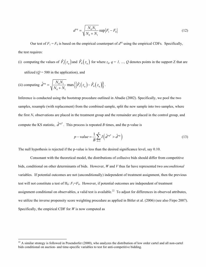
Our test of F1 = F0 is based on the empirical counterpart of deq using the empirical CDFs. Specifically,

the test requires:

(i) computing the values of ( )1 qF z and ( )0 qF z for where zq, q = 1, …, Q denotes points in the support Ζ that are

utilized (Q = 500 in the application), and

(ii) computing ( ) ( ){ }0 11 0

0 1

ˆ ˆ ˆmaxeqq q

N Nd F z F zN N

= −+

.

Inference is conducted using the bootstrap procedure outlined in Abadie (2002). Specifically, we pool the two

samples, resample (with replacement) from the combined sample, split the new sample into two samples, where

the first N1 observations are placed in the treatment group and the remainder are placed in the control group, and

compute the KS statistic, *ˆ eqd . This process is repeated B times, and the p-value is

( )*

1

1 ˆ ˆB

eq eq

bp value I d d

B =

− = >∑ (13)

The null hypothesis is rejected if the p-value is less than the desired significance level, say 0.10.

Consonant with the theoretical model, the distributions of collusive bids should differ from competitive

bids, conditional on other determinants of bids. However, W and V thus far have represented two unconditional

variables. If potential outcomes are not (unconditionally) independent of treatment assignment, then the previous

test will not constitute a test of H0: F1=F0. However, if potential outcomes are independent of treatment

assignment conditional on observables, a valid test is available.22 To adjust for differences in observed attributes,

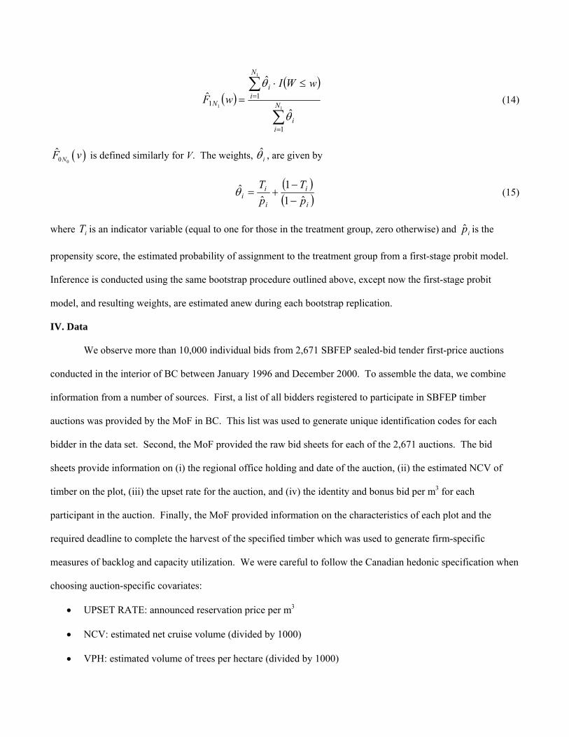
we utilize the inverse propensity score weighting procedure as applied in Bitler et al. (2006) (see also Firpo 2007).

Specifically, the empirical CDF for W is now computed as

22 A similar strategy is followed in Pesendorfer (2000), who analyzes the distribution of low order cartel and all non-cartel bids conditional on auction- and time-specific variables to test for anti-competitive bidding.

( )( )

∑

∑

=

=

≤⋅=

1

1

1

1

11

ˆ

ˆˆ

N

ii

N

ii

N

wWIwF

θ

θ (14)

( )00NF v is defined similarly for V. The weights, iθ , are given by

( )( )i

i

i

ii p

TpT

ˆ11

ˆˆ

−−

+=θ (15)

where iT is an indicator variable (equal to one for those in the treatment group, zero otherwise) and ip is the

propensity score, the estimated probability of assignment to the treatment group from a first-stage probit model.

Inference is conducted using the same bootstrap procedure outlined above, except now the first-stage probit

model, and resulting weights, are estimated anew during each bootstrap replication.

IV. Data

We observe more than 10,000 individual bids from 2,671 SBFEP sealed-bid tender first-price auctions

conducted in the interior of BC between January 1996 and December 2000. To assemble the data, we combine

information from a number of sources. First, a list of all bidders registered to participate in SBFEP timber

auctions was provided by the MoF in BC. This list was used to generate unique identification codes for each

bidder in the data set. Second, the MoF provided the raw bid sheets for each of the 2,671 auctions. The bid

sheets provide information on (i) the regional office holding and date of the auction, (ii) the estimated NCV of

timber on the plot, (iii) the upset rate for the auction, and (iv) the identity and bonus bid per m3 for each

participant in the auction. Finally, the MoF provided information on the characteristics of each plot and the

required deadline to complete the harvest of the specified timber which was used to generate firm-specific

measures of backlog and capacity utilization. We were careful to follow the Canadian hedonic specification when

choosing auction-specific covariates:

• UPSET RATE: announced reservation price per m3

• NCV: estimated net cruise volume (divided by 1000)

• VPH: estimated volume of trees per hectare (divided by 1000)

• LNVPT: log of estimated volume per tree

• LSPI: the average selling price index for timber harvested

• DC: deflated development costs (divided by NCV)

• SLOPE: weighted average slope

• BWDN: estimated percent of volume blown down

• BURN: estimated percent of volume burned

• CY: estimated percent of volume to be extracted via cable

• HP: estimated percent of volume to be extracted via helicopter

• HORSE: estimated percent of volume to be extracted via horse

• UTIL: estimated capacity utilization for firm i – ratio of current backlog of timber contracts in m3 to

maximum backlog of timber contracts in m3

• CYCLE: estimated cycle time for harvested timber

• LNB: natural log of the number of bidders.

In determining which bids to employ in the empirical analysis, we eliminated all auctions for which (i) the

designation was Category 2, (ii) the NCV of the plot was less than 1,000 m3, (iii) there were fewer than three bids

placed, and (iv) the sale method was other than a sealed-bid tender. This approach is consistent with the criteria

the BC government plans to use to estimate the hedonic pricing function discussed in Section II. Furthermore, we

eliminate any firm that places only one bid in the sample, as we would be unable to identify the individual fixed

effects for any such bidder. These selection criteria result in a sample of 6,353 observed bids placed by 847

different firms.

Summary statistics of the relevant variables are provided in Table 1. The statistics are provided for the

full sample of 6,353 bids, as well as by sub-sample depending on whether the bid is assumed to be part of a bid-

rigging scheme or not. We utilize two means of classifying bids as collusive or competitive at this point. For

purposes of utilizing the methods set forth in Case I and Case III, we postulate an auction-invariant and auction-

varying indicator of collusion, respectively.

As a starting point for identifying potentially collusive firms in the time-invariant models, we draw upon

previous theoretical and empirical literature identifying conditions likely to foster and sustain anti-competitive

outcomes. First, we examine the number of potential competitors in a given market and the frequency with which

these competitors bid. It is well understood that the likelihood of firms entering a collusive arrangement and the

stability of anti-competitive behavior conditional upon such agreement are directly related to the level of

concentration in a given market (Chamberlain 1929; Bain 1951; Dolbear et al. 1968). More recently, authors

have considered not only the level of concentration in a given market, but also the frequency with which firms

interact (Benoit and Krishna 1985; Fudenberg and Maskin 1986).

Using the theoretical studies outlined above as a guide, we settled on the following set of decision rules

for selecting pairs of firms whose bidding behavior warrant further examination: (i) the pair must have jointly

submitted bids in at least six auctions during the sample period; (ii) each firm must have won at least one of these

auctions; and (iii) there must be a fairly even balance in the pairwise rank of submitted bids between the two

firms.23 Based upon these selection criteria, we classify 130 firms (2,617 total bids) as belonging to the treatment

group. To identify suspected collusive bids in the time-varying models, we denote a bid as collusive if it is placed

by a firm suspected of engaging in bid-rigging under the auction-invariant classification in an auction in which at

least one other firm also suspected of being engaged in bid-rigging participated. Based upon this criterion, we

classify 1,475 total bids (distributed among 127 firms) as belonging to the treatment group in the auction-varying

specification.

Throughout the empirical analysis, we assume that our bid data are drawn from IPV auctions. This is

intuitively appealing for these data considering that bidders face different capacity constraints, suggesting that

idiosyncratic, firm-specific cost factors are more important than plot-specific uncertain costs. Furthermore,

bidders contract with different mills to sell harvested timber at some predetermined price. Since we would expect

price quotes to differ across mills, this implies independent and private expectations over revenues across loggers. 23 Our selection criteria implicitly assume that the cartel strategy followed is one whereby all but a single, predetermined cartel member submits ‘phantom’ bids. There are alternate cartel strategies whereby only a single cartel firm participates in a given auction. Such a cartel would go undetected via our selection criteria. Such omission would make the Bajari and Ye (2003) identification strategy conservative provided there is no systematic selection issue. On the other hand, if there exists an unaccounted for deterministic process by which firms organize bids into competitive and collusive auctions, then any identification strategy that relies upon a comparison of estimates from reduced form bid functions across competitive and cartel designations is potentially biased.

V. Empirical Results

Auction-Invariant Treatment Assignment

Case I.

Empirical results from a variety of tests assuming that the underlying data are generated according to

(DGP1) are presented in Tables 2 – 5. The first set of results displayed in Table 2 present estimates obtained from

estimating equation (2).24 The first specification uses the total bid as the dependent variable. Because there

appears to be a selection issue whereby suspected bid-rigging firms tend to participate in auctions with higher

upset rates, we utilize a second specification that includes the upset rate as a covariate. The final specification

uses the bonus bid as the dependent variable. Assuming τ < 0, under assumptions (A1), (A3) – (A4), a negative

and statistically significant firm effect is evidence of collusive behavior by that particular firm. In total, 247 (226)

of the 847 firm effects are negative and statistically significant at the p < 0.10 level using the total bid as the

dependent variable and not conditioning (conditioning) on the upset rate; 259 firm effects are negative and

statistically significant using the bonus bid as the dependent variable. In contrast, only 105 (83) of the 847 firm

effects are positive and statistically significantly at the p < 0.10 level using the total bid as the dependent variable

and not conditioning (conditioning) on the upset rate; 75 firm effects are positive and significant using the bonus

bid as the dependent variable.25

Recall that under our maintained assumptions, a negative and significant fixed effect yields the identity of

a treated observation (firm). Hence, we are able to examine whether those firms suspected under our criteria of

possibly being cartel members are more likely to have a negative and significant fixed effect than a competitive

designated counterpart. As noted in Table 2, across all three models, the percentage of firms designated as

possible cartel members with negative and significant fixed effects is greater than those observed for

competitively designated counterparts. For example, approximately 55.4 percent (72 out of 130) of the firms

identified as a possible cartel members have negative and significant fixed effects when the bonus bid is the 24 We estimated equation (1) omitting a constant term from the model. Results from these models are available upon request and provide minimal evidence of collusion as less than two percent fixed effects were negative and significant. However, assumption (A2) – the absence of a constant term – seems implausible for the data. 25 Since the fixed effects estimates are random variables, we would expect about five percent of the estimates to be negative and significant at the p < 0.10 level in the absence of treatment. We observe negative and significant effects for approximately one-third of our sample, suggesting a non-negligible portion of bidders received treatment. In contrast, only nine to twelve percent of the estimated fixed effects are positive and statistically significant.

dependent variable. In contrast, only 26.8 percent (187 of 717) of the firms identified as competitive have

negative and significant fixed effects with this 28.6 percent difference in percentages significant at the p < 0.01

level using a two-sample test of proportions. Furthermore, we are able to examine the percentage of firms that

have negative and significant fixed effects in all three model specifications. In total, 21.5 percent (28 of 130) of

the firms designated as a possible cartel member have estimated fixed effects that are negative and significant in

all models. For competitively designated firms, this percentage falls to 14.8 percent (106 of 717) with this 6.7

percent difference significant at the p < 0.05 level using a two-sample test of proportions. The fact that the results

are consistent with our prior provides some comfort that the results are not simply reflecting other sources of

firm-specific, unobserved heterogeneity.26

Table 3 contains results from the conditional independence tests – requiring only assumption (A1) – using

the three prior specifications from Table 3.27 Across all model specifications, we reject the null of conditional

independence for 23.4 to 29.6 percent of all bidder pairs that submit bids in at least four common auctions. For

pairs of firms that submit bids in fewer than eight common auctions, these percentages range from 4.1 percent (for

firms that jointly participate in four auctions in our model of the bonus bid) to 30.5 percent (for firms that jointly

participate in five auctions in our model of the bonus bid). For firms that participate in eight or more common

auctions, the fraction of bidder pairs for which we reject conditional independence ranges from 33.3 percent (for

the bonus bids of firm pairs with eleven repetitions) to a high of 80 percent (for the total bids of firms with ten

repetitions). If we restrict the analysis to only those firms designated as a possible cartel, we are able to reject the

null of conditional independence for 30.8 to 41.5 percent of the 130 bidder pairs. In contrast, we are able to reject

the null of conditional independence for only 11.4 to 15.6 percent of the 96 competitively designated bidder pairs.

Thus, relaxing (A2) – (A4) provides additional empirical evidence consistent with collusive behavior, as well as

our prior concerning likely cartel members.

26 While additional data on firm-specific attributes would enable us to determine whether our results are reflect other sources of unobserved firm heterogeneity, we do not have any additional information on such attributes for the full data sample. 27 Note, Bajari and Ye (2003) test for conditional independence after estimating a regression model that includes fixed effects for only a subset of firms and test for residual correlation conditional largely on the observables, X. We believe that testing for independence conditional on firm effects and X is a more conservative test of collusion.

Table 4 contains the next set of results, obtained from estimating (DGP1) replacing Di with iD% , where

iD% is the auction-invariant classification defined in the previous section and utilized in Table 1. As in Table 2,

we estimate three specifications. In all cases, a negative and statistically significant coefficient on iD% is evidence

of collusion. In the two specifications using the total bid as the dependent variable, the coefficient on iD% is

positive (and statistically significant in the first specification which does not condition on the announced upset

rate). When we examine the bonus bid in the third specification, the coefficient of iD% is negative but not

statistically significant at conventional levels. Nevertheless, the final specification focusing solely on the bonus

bid yields evidence consonant with our suspicion that alleged non-competitive firms tend to participate in higher

stakes auctions with larger upset rates.

While the third specification yields a coefficient on iD% of the ‘correct’ sign if collusion is present in the

sample, since iD% is likely measured with error, the coefficient is attenuated toward zero. To (potentially)

improve on the estimate of τ, we define a second indicator of collusive firms, iD′% and provide estimates of

equation (3) in Table 5. In creating iD′% , we draw upon the theoretical literature that examines the effect of multi-

market contact on the stability of collusion (Bernheim and Whinston 1990; Spagnolo 1999; Matsushima 2001).

In BC, loggers (Category 1 bidders) interact in the SBFEP auction market and as contract laborers for

firms that hold long-term tenure licenses. As such, we would expect that bidders who interact in both of these

markets are more likely to collude. Unfortunately, our data do not permit us to identify which bidders contract

with any given tenure holder. Instead, we create an indicator variable that proxies for the likelihood that any

subset of firms would interact in this labor market and use this proxy as a second potential indicator of collusion.

In creating this proxy, we note that the annual allowable cuts (AAC) for tenure contracts are heavily

concentrated across four major firms: Canadian Forest Products Ltd, Slocan Forest Products Ltd, Weyerhaeuser

Company Ltd, and West Fraser Mills Ltd. While these firms employ a number of full-time loggers, they also

outsource for a large percentage of any harvest labor needs. As such, we hypothesize that bidders located in a

district where these firms have a ‘large’ total AAC would be more likely to engage in the type of multi-market

contact that has been shown to facilitate collusion. Making use of GIS tools, we constructed detailed information

about the geographic location and AAC volume for tenure holdings of these firms.28 We were able to identify

twelve (out of 31) districts in the interior region of BC where these four firms have combined AACs of over

400,000 m3.

To generate data on the geographic location of bidders, we combined information from several sources.

First, a list of all bidders currently registered to participate in SBFEP timber auctions was provided by the MoF.

The registration data contained home localities for approximately two-thirds of the 1,771 bidders in the initial

sample. We hand coded the location of all remaining bidders by searching the BC yellow pages (logging

firm/companies) or white pages (individual loggers) and were able to acquire geographic locations for all but

roughly 350 bidders. Making use of GIS tools, we identified 13 cities located in these 12 districts where there

were more than 15 registered bidders. Thus, our second indicator is a binary variable that equals one for any firm

located in one of these cities; zero otherwise.

In Table 5, the parameter of interest is the coefficient on the variable indicating 1i iD D′= =% % . In this case,

the final two estimates are negative, with the coefficient in the final specification gaining statistical significance at

the p < 0.10. These estimates suggest two conclusions. First, there is minimal evidence of collusion: we find

directional (but not statistical) support for anti-competitive bidding when examining total bids conditioned on the

announced upset rate and statistical support for anti-competitive bidding when examining bonus bids. Second, our

evidence suggests that suspected cartel firms select into higher stakes auctions with larger announced upset rates.

In sum, then, if the data are generated according to (DGP1), we find empirical evidence consistent with

collusion by some subset of bidders. Approximately one-third of the firm effects are consistent with collusion in

the “deviations specification” in Table 2, with these percentages greater for suspected cartel members across all

model specifications. Furthermore, inference based on the notion of conditional independence suggests the

presence of anti-competitive behavior by an economically meaningful sub-sample of firms designated as a suspect

bidding pair. Finally, the lower bound (in absolute value) estimate of τ is negative, albeit statistically

28 Intuitively, our second indicator relies upon variation across geographic space that could theoretically impact the stability of a collusive arrangement but should not impact the unobserved component of individual valuations. We use a similar strategy in creating our second indicator for the auction-varying model described in Case III below.

insignificant, in Table 4 when analyzing the bonus bid using our main hypothesized indicator of anti-competitive

firms. Moreover, when we introduce a second hypothesized indicator of anti-competitive firms, our estimate of τ

is negative and statistically significant when analyzing bonus bids.

While one cannot eliminate the possibility that our results reflect other dimensions of unobserved

heterogeneity across firms, rather than differences in bid-rigging behavior, the fact that our methods yield results

consistent with our prior concerning suspected colluders is comforting. Moreover, if we examine the consistency

of the results across the fixed effects and conditional independence tests, we find additional support for our

methodology. For example, in the specifications using the bonus bid, we reject conditional independence for 55

of 226 firm pairs we observe bidding together in at least four auctions. Of these 55, 26 pairs (47.2 percent)

contain firms that are both found to have negative and statistically significant firm effects in Table 2. In contrast,

of the 171 firm pairs for which we fail to reject the conditional independence assumption, 52 pairs (30.4 percent)

contain firms that are both found to have negative and statistically significant firm effects in Table 2. This 16.8

percent difference in percentages is significant at the p < 0.03 level using a two-sample test of proportions.

Case II.

Under (DGP2) the only detection algorithm that is available in the current application is the test of

exchangeability based on estimation of (5). Since assumption (B2) is not met with our data, tests based on

estimation of (4) are not feasible. Results using the total bid as the dependent variable and excluding the upset

rate from the conditioning set are presented in Table 6. The primary result of interest is the test for the constancy

of the coefficient vector across the samples with 1 and 0i iD D= =% % (i.e., suspected colluding and non-colluding

firms). Here, we easily reject the null that βnon-collude = βcollude at the p < 0.01 confidence level.29 Furthermore, the

average predicted markup in bids - conditioned on observed covariates - is greater for firms designated as

competitive, consonant with the assumption of ‘phantom’ bids among the cartel bids. Given the theoretical

framework used to conceptualize the bidding behavior of firms, this constitutes further evidence of collusion,

provided that assumption (B1) holds.

Auction-Varying Treatment Assignment 29 Moreover, if we condition on the upset rate or utilize the bonus bid as the dependent variable, we continue to reject the null of equal coefficients at the p < 0.05 level. All results not reported are available from the authors upon request.

Case III.

Under (DGP3) the only test for collusion available is to estimate (7) using itD% , the auction-varying

classification of collusive bids. Results are provided in Table 7 for our three model specifications. In all three

specifications, the coefficient on itD% is positive and statistically significant. Since measurement error only

attenuates the estimates, this provides evidence against the presence of collusion in the data. To (potentially)

reduce the measurement error, Table 8 provides estimates of (8), which utilize two mis-measured indicators of

auction-varying collusion. Our second indicator is a binary variable that equals one for any bid placed in an

auction held in one of the twelve districts in the interior of British Columbia where Canadian Forest Products Ltd,

Slocan Forest Products Ltd, Weyerhaeuser Company Ltd, and West Fraser Mills Ltd have combined AACs of

over 400,000 m3; zero otherwise. Since at least some firms place bids in multiple districts, this indicator is not

constant across auctions for all firms.

In Table 8, the parameter of interest corresponds to the coefficient on the variable indicating

1it itD D′= =% % . These estimates suggest two conclusions. First, there is some, albeit weak, evidence of collusion.

The estimated coefficient on our indicator of collusion is negative for our second and third model specifications -

with the later estimate statistically significant at the p < 0.01 level. Second, the fact that utilizing itD′% did not

improve the lower bounds reported in Table 7 (and even caused the estimated treatment effects to switch sign for

two of the three specifications) indicates that the measurement errors associated with itD% and itD′% are correlated

conditional on treatment assignment.

In sum, if the data are generated according to (DGP3), the methods utilized provide only modest evidence

of collusion in the data. Nonetheless, there is some evidence of anti-competitive behavior in that the lower bound

(in absolute value) estimate of τ is negative in two of our three specifications and statistically significant in a

model of bonus bids.

Case IV.

As in Case II, if (DGP4) is assumed to characterize the underlying data, the only test available in the

current application is the test of exchangeability based on estimation of (10) since assumption (D2) is not met in

our data. Results using the total bid as the dependent variable and excluding the upset rate from the conditioning

set are presented in Table 9. The primary result of interest is the test for the constancy of the coefficient vector

across the samples with 1 and 0it itD D= =% % (i.e., suspected colluding and non-colluding bids). Here, we easily

reject the null that βnon-collude = βcollude at the p < 0.01 confidence level; we also reject the null of equality at the p <

0.01 level if we condition on the upset rate or utilize the bonus bid as the dependent variable. Furthermore, the

predicted mark-ups of suspected collusive bids are lower on average than for the suspected competitive bids.

Given our theoretical framework, these results provide empirical evidence consonant with collusion by some

subset of firms, provided that (D1) holds.

Distributional Analysis

The final set of results is provided in Table 10. We report the value of deq and the corresponding p-value

associated with the null of equality of the distributions for many comparisons. Panels I and II compare

distributions of the total bid, where the distributions adjusted for covariates in Panel II are obtained by including

the upset rate in the conditioning set included in the propensity score estimation. Panel III examines the the

distributions of the bonus bid. In all three panels, we divide the sample into collusive and competitive bids via

four methods. First, we compare the distribution of bids by firms with 1iD =% versus firms with 0iD =% (see

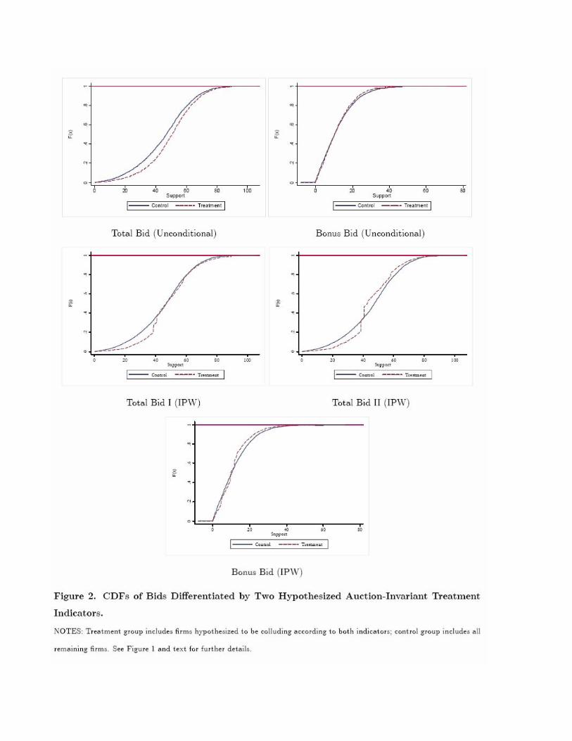
Figure 1).30 Second, we compare the distribution of bids by firms with 1i iD D′= =% % versus all other firms (see

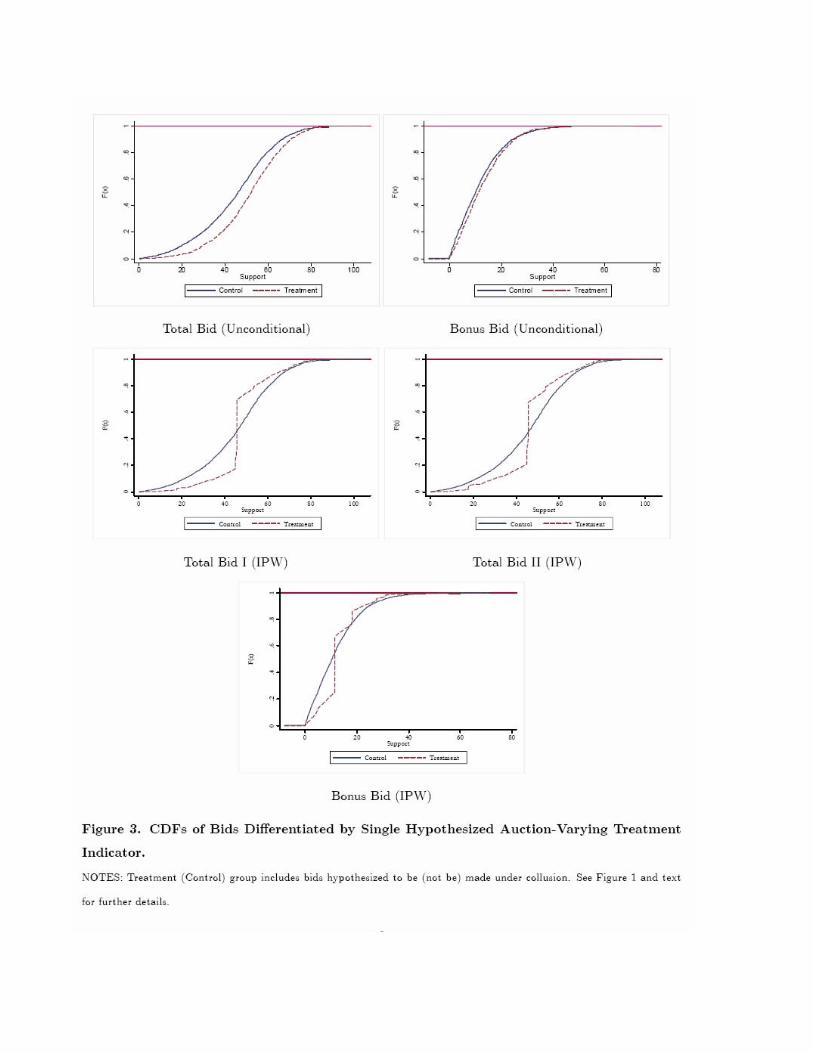
Figure 2). Third, we compare the distribution of bids for which 1itD =% versus bids for which 0itD =% (see Figure

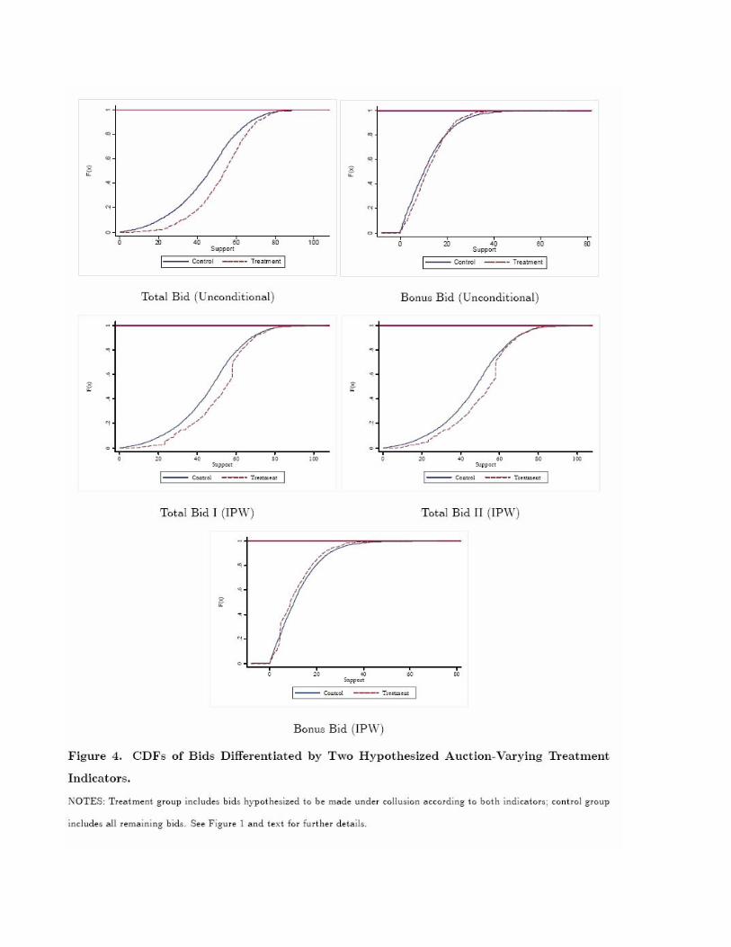
3). Finally, we compare the distribution of bids for which 1it itD D′= =% % versus all other bids (see Figure 4).

The basic results are easily summarized: in 19 of the 20 unique comparisons, we reject the null of equality

of the distributions at the p < 0.05 confidence level.31 Moreover, we reject equality of the distributions adjusting

for covariates at the p < 0.01 confidence level in every case. Finally, analyzing the figures, especially Figure 4

(bottom panel), reveals that the distribution of suspected collusive bids lies to the left of the corresponding

30 Note, the use of the inverse propensity score weighting generates the apparent discrete jumps in the empirical CDFs. The jumps arise due to the large weight assigned to some control group observations to compensate for the greater number of comparable treated observations (Firpo 2007). 31 The unconditional tests in Panels I and II are identical.

distribution of presumed competitive bids over the majority of the support. This provides some evidence at the

distributional level that ‘phantom’ bids are present.

Summation

Given the difficult nature of the current problem – identifying treatment assignment when it is unobserved

– we pursue several tests based on different underlying data structures. Tests based on fixed effects models (Case

I), conditional independence (Case I), and exchangeability (Cases II and IV) provide evidence consistent with

collusion by some subset of bidders. The distributional tests (Case V) are also in line with these parametric tests,

providing further evidence suggestive of collusive behavior. Tests based on estimating the treatment effect and

comparing its sign to the theoretically predicted negative effect utilizing mis-measured treatment indicators

(Cases I and III) yield weaker results; some positive and some negative point estimates, with the negative point

estimates being statistically significant in a limited number of cases (although the estimates represent lower

bounds). Thus, we find mixed evidence as to whether observed behavior in SBFEP auctions is consistent with a

model of competitive bidding.

That being the case, we wish to avoid making normative claims concerning the current softwood lumber

trade dispute. For example, it is not the purpose of this study to assess whether collusion renders the proposed

timber pricing system less than satisfactory. Future work should determine whether the evidence of collusion is

sufficient to undermine the integrity of the proposed timber pricing system and assess the performance of this

system relative to alternative mechanisms for pricing standing timber.

IV. Conclusion

In this study we make use of the program evaluation structure, to provide a framework to identify the

treatment assignment (collusive or competitive) of observations given data on outcomes (bids). While we design

our specifics tests to detect collusion in first-price auctions, we view this empirical modeling approach as having

numerous economic applications outside of this specific context – i.e., principal agent and detection problems of

the sort commonly confronting micro-econometricians.

We utilize our methodology by examining bidder behavior in SBFEP timber auctions in British Columbia

for the period 1996 – 2000. Understanding bidder behavior in these auctions is integral to the resolution of the

U.S.-Canadian softwood lumber dispute. As part of this resolution, British Columbia is to auction off cutting

rights on a portion of its federal land, estimate a hedonic price function to determine the shadow values of the

plot’s characteristics, and use the results to price cutting rights on all non-auctioned federal lands. For this

solution to lead to an agreement of “changed circumstance” (lifting of the CVD/AD), British Columbia must

show that this method provides a viable and robust market. In this sense, it is vital that collusion does not

undermine the integrity of the auctions. In sum, our data provide mixed evidence as to whether the observed bids

arise from a model of perfectly competitive behavior.

References

Abadie, A. (2002), “Bootstrap Tests for Distributional Treatment Effects in Instrumental Variable Models,” Journal of the American Statistical Association, 97, 284-292.

Aigner, D.J. (1973), “Regression with a Binary Independent Variable Subject to Errors of Observation,” Journal

of Econometrics, 1, 49-60. Bain, J. (1951), “Relation of Profit Rate to Industry Concentration: American Manufacturing, 1936-1940,”

Quarterly Journal of Economics, 65, 293-324. Bajari, P. and L. Ye (2003), “Deciding between Competition and Collusion,” Review of Economics and Statistics. Baldwin, L., R. Marshall, and J.-F. Richard (1997), “Bidder Collusion at Forest Service Timber Sales,” Journal of

Political Economy, 105, 657-699. Benoit, J.-P. and V. Krishna (1985), “Finitely Repeated Games,” Econometrica, 53, 890-904. Bernheim, B.D. and M. Whinston (1990), “Multimarket Contact and Collusive Behavior,” RAND Journal of

Economics, 21, 1-26. Bitler, M.P., J.B. Gelbach, and H.W. Hoynes (2006), “What Mean Impacts Miss: Distributional Effects of

Welfare Reform Experiments,” American Economic Review, 96, 988-1012. Black, D.A., M.C. Berger, and F.A. Scott (2000), “Bounding Parameter Estimates with Nonclassical

Measurement Error,” Journal of the American Statistical Association, 95, 739-748. Bollinger, C.R. (1996), “Bounding Mean Regressions When a Binary Regressor is Mismeasured,” Journal of

Econometrics, 73, 387-399. Cameron, A.C. and P.K. Trivedi (2005), Microeconometrics: Methods and Applications, NY, NY: Cambridge

University Press. Chamberlain, E. (1929), “Duopoly: Value Where Sellers are Few,” Quarterly Journal of Economics, 43, 63-100. Dolbear, F.T., L.B. Lowe, G. Bowman, A. Lieberman, E. Prescott, F. Rueter, and R. Sherman (1968), “Collusion

in Oligopoly: An Experiment on the Effects of Numbers and Information,” Quarterly Journal of Economics, 82, 240-259.

Firpo, S. (2007), “Efficient Semiparametric Estimation of Quantile Treatment Effects,” Econometrica, 75, 259-

276. Fudenberg, D. and E. Maskin (1986), “The Folk Theorem in Repeated Games with Discounting and with

Incomplete Information,” Econometrica, 54, 533-554. Graham, D. and R. Marshall (1987), “Collusive Bidder Behavior at Single-Object Second-Price and English

Auctions,” Journal of Political Economy, 95, 1217-1239. Jacob, B.A. and S.D. Levitt (2003), “Rotten Apples: An Investigation of the Prevalence and Predictors of Teacher

Cheating,” Quarterly Journal of Economics, 118, 843-877.

Kreider, B. and J.V. Pepper (2006), “Inferring Disability Status from Corrupt Data,” unpublished manuscript, Iowa State University.

Matsushima, H. (2001), “Multimarket Contact, Imperfect Monitoring, and Implicit Collusion,” Journal of

Economic Theory, 98, 158-178. Pesendorfer, M. (2000), “A Study of Collusion in First Price Auctions,” Review of Economic Studies, 67, 381-

411. Porter, R. and D. Zona (1993), “Detection of Bid-Rigging in Procurement Auctions,” Journal of Political

Economy, 101, 518-538. Porter, R. and D. Zona (1999), “Ohio School Milk Markets: An Analysis of Bidding,” Rand Journal of

Economics, 30, 263-288. Spagnolo, G. (1999), “On Interdependent Supergames: Multimarket Contact, Concavity, and Collusion,” Journal

of Economic Theory, 89, 127-139.

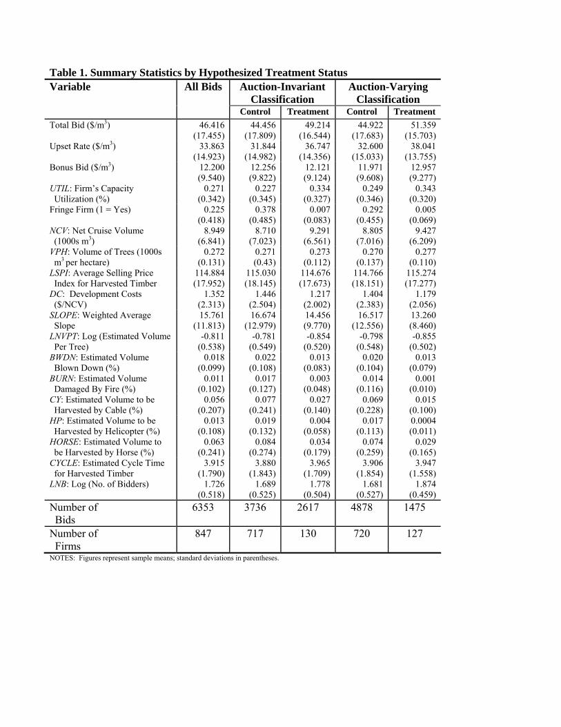
Table 1. Summary Statistics by Hypothesized Treatment Status Variable All Bids Auction-Invariant

Classification Auction-Varying

Classification Control Treatment Control Treatment Total Bid ($/m3) 46.416

(17.455) 44.456

(17.809)49.214

(16.544)44.922

(17.683)51.359

(15.703) Upset Rate ($/m3) 33.863

(14.923) 31.844

(14.982)36.747

(14.356)32.600

(15.033)38.041

(13.755) Bonus Bid ($/m3)

12.200 (9.540)

12.256 (9.822)

12.121 (9.124)

11.971 (9.608)

12.957 (9.277)

UTIL: Firm’s Capacity Utilization (%)

0.271 (0.342)

0.227 (0.345)

0.334 (0.327)

0.249 (0.346)

0.343 (0.320)

Fringe Firm (1 = Yes) 0.225 (0.418)

0.378 (0.485)

0.007 (0.083)

0.292 (0.455)

0.005 (0.069)

NCV: Net Cruise Volume (1000s m3)

8.949 (6.841)

8.710 (7.023)

9.291 (6.561)

8.805 (7.016)

9.427 (6.209)

VPH: Volume of Trees (1000s m3 per hectare)

0.272 (0.131)

0.271 (0.43)

0.273 (0.112)

0.270 (0.137)

0.277 (0.110)

LSPI: Average Selling Price Index for Harvested Timber

114.884 (17.952)

115.030 (18.145)

114.676 (17.673)

114.766 (18.151)

115.274 (17.277)

DC: Development Costs ($/NCV)

1.352 (2.313)

1.446 (2.504)

1.217 (2.002)

1.404 (2.383)

1.179 (2.056)

SLOPE: Weighted Average Slope

15.761 (11.813)

16.674 (12.979)

14.456 (9.770)

16.517 (12.556)

13.260 (8.460)

LNVPT: Log (Estimated Volume Per Tree)

-0.811 (0.538)

-0.781 (0.549)

-0.854 (0.520)

-0.798 (0.548)

-0.855 (0.502)

BWDN: Estimated Volume Blown Down (%)

0.018 (0.099)

0.022 (0.108)

0.013 (0.083)

0.020 (0.104)

0.013 (0.079)

BURN: Estimated Volume Damaged By Fire (%)

0.011 (0.102)

0.017 (0.127)

0.003 (0.048)

0.014 (0.116)

0.001 (0.010)

CY: Estimated Volume to be Harvested by Cable (%)

0.056 (0.207)

0.077 (0.241)

0.027 (0.140)

0.069 (0.228)

0.015 (0.100)

HP: Estimated Volume to be Harvested by Helicopter (%)

0.013 (0.108)

0.019 (0.132)

0.004 (0.058)

0.017 (0.113)

0.0004 (0.011)

HORSE: Estimated Volume to be Harvested by Horse (%)

0.063 (0.241)

0.084 (0.274)

0.034 (0.179)

0.074 (0.259)

0.029 (0.165)

CYCLE: Estimated Cycle Time for Harvested Timber

3.915 (1.790)

3.880 (1.843)

3.965 (1.709)

3.906 (1.854)

3.947 (1.558)

LNB: Log (No. of Bidders) 1.726 (0.518)

1.689 (0.525)

1.778 (0.504)

1.681 (0.527)

1.874 (0.459)

Number of Bids

6353 3736 2617 4878 1475

Number of Firms

847 717 130 720 127

NOTES: Figures represent sample means; standard deviations in parentheses.

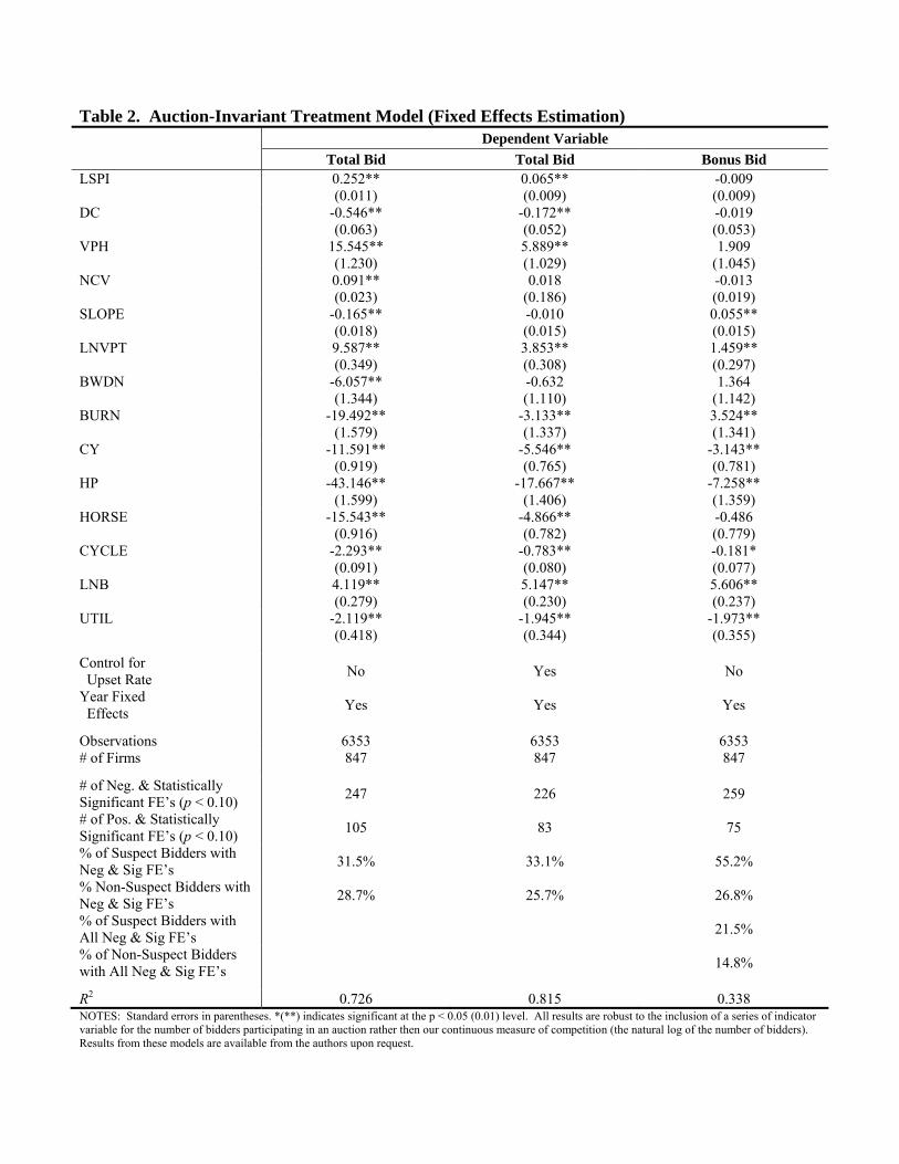
Table 2. Auction-Invariant Treatment Model (Fixed Effects Estimation) Dependent Variable Total Bid Total Bid Bonus Bid LSPI 0.252**

(0.011) 0.065** (0.009)

-0.009 (0.009)

DC -0.546** (0.063)

-0.172** (0.052)

-0.019 (0.053)

VPH 15.545** (1.230)

5.889** (1.029)

1.909 (1.045)

NCV 0.091** (0.023)

0.018 (0.186)

-0.013 (0.019)

SLOPE -0.165** (0.018)

-0.010 (0.015)

0.055** (0.015)

LNVPT 9.587** (0.349)

3.853** (0.308)

1.459** (0.297)

BWDN -6.057** (1.344)

-0.632 (1.110)

1.364 (1.142)

BURN -19.492** (1.579)

-3.133** (1.337)

3.524** (1.341)

CY -11.591** (0.919)

-5.546** (0.765)

-3.143** (0.781)

HP -43.146** (1.599)

-17.667** (1.406)

-7.258** (1.359)

HORSE -15.543** (0.916)

-4.866** (0.782)

-0.486 (0.779)

CYCLE -2.293** (0.091)

-0.783** (0.080)

-0.181* (0.077)

LNB 4.119** (0.279)

5.147** (0.230)

5.606** (0.237)

UTIL -2.119** (0.418)

-1.945** (0.344)

-1.973** (0.355)

Control for Upset Rate No Yes No

Year Fixed Effects Yes Yes Yes

Observations 6353 6353 6353 # of Firms 847 847 847

# of Neg. & Statistically Significant FE’s (p < 0.10) 247 226 259

# of Pos. & Statistically Significant FE’s (p < 0.10) 105 83 75

% of Suspect Bidders with Neg & Sig FE’s 31.5% 33.1% 55.2%

% Non-Suspect Bidders with Neg & Sig FE’s 28.7% 25.7% 26.8%

% of Suspect Bidders with All Neg & Sig FE’s 21.5%

% of Non-Suspect Bidders with All Neg & Sig FE’s 14.8%

R2 0.726 0.815 0.338 NOTES: Standard errors in parentheses. *(**) indicates significant at the p < 0.05 (0.01) level. All results are robust to the inclusion of a series of indicator variable for the number of bidders participating in an auction rather then our continuous measure of competition (the natural log of the number of bidders). Results from these models are available from the authors upon request.

Table 3. Percentage of Bidder Pairs Failing Tests of Conditional Independence Total Bid

(No Upset Rate) Total Bid

(Control for Upset) Bonus Bid

4 Repetitions 6.9% (5 out of 72)

6.9% (5 out of 72)

4.1% (3 out of 72)

5 Repetitions 27.8% (10 out of 36)

22.2% (8 out of 36)

30.5% (11 out of 36)

6 Repetitions 29.0% (9 out of 31)

16.1% (5 out of 31)

19.3% (6 out of 31)

7 Repetitions 23.1% (6 out of 26)

23.1% (6 out of 26)

26.9% (7 out of 26)

8 Repetitions 47.6% (10 out of 21)

42.9% (9 out of 21)

47.6% (10 out of 21)

9 Repetitions 66.7% (8 out of 12)

58.3% (7 out of 12)

58.3% (7 out of 12)

10 Repetitions 80% (8 out of 10)

50% (5 out of 10)

50% (5 out of 10)

11 Repetitions 50% (3 out of 6)

33.3% (2 out of 6)

33.3% (2 out of 6)

12+ Repetitions 66.7% (8 out of 12)

50% (6 out of 12)

58.3% (7 out of 12)

All Firm Pairs 29.6% (67 out of 226)

23.4% (53 out of 226)

25.7% (58 out of 226)

Suspect Firm Pairs Only 41.5% (54 of 130)

30.8% (40 of 130)

32.3% (42 of 130)

Non-Suspect Firm Pairs Only

15.6% (15 of 96)

11.4% (11 of 96)

13.5% (13 of 96)

Reject CI in All Models – Suspect Pairs Only

30.0% (39 of 130)

Reject CI in All Models – Non-Suspect Pairs Only

9.4% (9 of 96)

NOTES: Cell entries report the percentage of firm pairings that submit bids which fail to demonstrate conditional independence at the p < 0.05 level of significance. Tests for conditional independence use the Fisher transformation on the estimated residuals from the fixed effects auction invariant treatment model (Table 3). For example, 4.1% of the unique bidder pairs that compete against one another in four auctions submit bonus bids that are not conditionally independent.

Table 4. Auction-Invariant Treatment Model (Random Effects Estimation): Single Hypothesized Treatment Indicator Dependent Variable Total Bid Total Bid Bonus Bid Constant 22.371**

(1.462) 5.492** (1.188)

-1.176 (1.187)

LNB 4.448** (0.265)

5.593** (0.214)

6.011** (0.219)

UTIL -1.806** (0.397)

-1.617** (0.319)

-1.644** (0.329)

Control for Fringe Firms

-1.480** (0.572)

-0.953** (0.402)

-0.750* (0.404)

Collude (1 = Yes)

1.617** (0.711)

0.021 (0.481)

-0.465 (0.479)

Plot Characteristics Yes Yes Yes Upset Rate No Yes No Year Fixed Effects Yes Yes Yes Total Observations 6353 6353 6353 Average # of Bids per Firm

7.5 7.5 7.5

R2 0.62 0.77 0.21 NOTES: See Table 2.

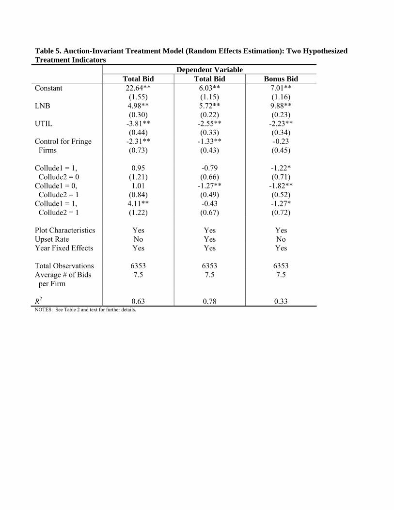
Table 5. Auction-Invariant Treatment Model (Random Effects Estimation): Two Hypothesized Treatment Indicators Dependent Variable Total Bid Total Bid Bonus Bid Constant 22.64**

(1.55) 6.03** (1.15)

7.01** (1.16)

LNB 4.98** (0.30)

5.72** (0.22)

9.88** (0.23)

UTIL -3.81** (0.44)

-2.55** (0.33)

-2.23** (0.34)

Control for Fringe Firms

-2.31** (0.73)

-1.33** (0.43)

-0.23 (0.45)

Collude1 = 1, Collude2 = 0

0.95 (1.21)

-0.79 (0.66)

-1.22* (0.71)

Collude1 = 0, Collude2 = 1

1.01 (0.84)

-1.27** (0.49)

-1.82** (0.52)

Collude1 = 1, Collude2 = 1

4.11** (1.22)

-0.43 (0.67)

-1.27* (0.72)

Plot Characteristics Yes Yes Yes Upset Rate No Yes No Year Fixed Effects Yes Yes Yes Total Observations 6353 6353 6353 Average # of Bids per Firm

7.5 7.5 7.5

R2 0.63 0.78 0.33 NOTES: See Table 2 and text for further details.

Table 6. Auction-Invariant Treatment Model (Random Effects Estimation): Exchangeability Test Sample All Firms Non-Colluding

Firms Colluding

Firms Constant 22.986**

(1.438) 23.058** (1.837)

20.521** (2.275)

LSPI 0.275** (0.009)

0.269** (0.013)

0.292** (0.015)

DC -0.658** (0.059)

-0.746** (0.071)

-0.474** (0.105)

VPH 16.324** (1.183)

13.309** (1.364)

25.635** (2.341)

NCV 0.103** (0.021)

0.107** (0.027)

0.082** (0.035)

SLOPE -0.163** (0.017)

-0.117** (0.022)

-0.234** (0.027)

LNVPT 8.462** (0.325)

7.532* (0.418)

8.656** (0.517)

BWDN -7.610** (1.285)

-5.504* (1.525)

-13.683** (2.381)

BURN -20.316** (1.376)

-19.545** (1.480)

-23.626** (3.918)

CY -12.867** (0.854)

-12.846** (1.011)

-14.432** (1.666)

HP -43.804** (1.350)

-43.094** (1.499)

-43.586** (3.316)

HORSE -16.407** (0.749)

-15.294** (0.896)

-16.973** (1.327)

CYCLE -2.350** (0.084)

-2.187** (0.110)

-2.662** (0.129)

LNB 4.447** (0.265)

4.089** (0.346)

4.995** (0.410)

UTIL -1.770** (0.397)

-1.700** (0.519)

-2.200** (0.616)

Control for Fringe Firms -2.039** (0.517)

-1.578** (0.599)

-1.999 (2.739)

Year Fixed Effects Yes Yes Yes Observations 6353 3736 2617 Number of Firms 847 717 130 Average Bids per Firm 7.5 5.2 20.1 R2 0.620 0.622 0.620 Predicted Markup:

upsetux ˆˆ +β

2.953

3.605

2.009

H0: βnon-collude = βcollude

p = 0.00

NOTES: Dependent variable is total bid. When the upset rate is included as a regressor, the p-value for the test of exchangeability is p=0.02. When the bonus bid is the dependent variable, the p-value is p=0.02 as well. See Table 2 for further details.

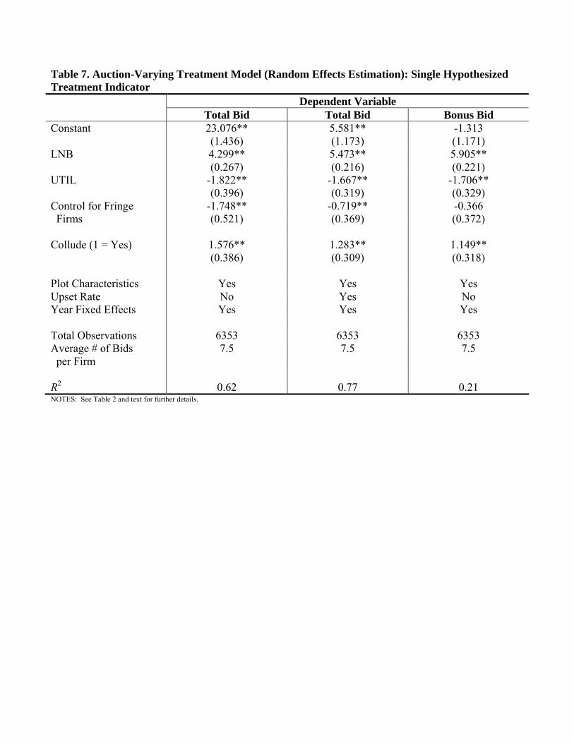
Table 7. Auction-Varying Treatment Model (Random Effects Estimation): Single Hypothesized Treatment Indicator Dependent Variable Total Bid Total Bid Bonus Bid Constant 23.076**

(1.436) 5.581** (1.173)

-1.313 (1.171)

LNB 4.299** (0.267)

5.473** (0.216)

5.905** (0.221)

UTIL -1.822** (0.396)

-1.667** (0.319)

-1.706** (0.329)

Control for Fringe Firms

-1.748** (0.521)

-0.719** (0.369)

-0.366 (0.372)

Collude (1 = Yes)

1.576** (0.386)

1.283** (0.309)

1.149** (0.318)

Plot Characteristics Yes Yes Yes Upset Rate No Yes No Year Fixed Effects Yes Yes Yes Total Observations 6353 6353 6353 Average # of Bids per Firm

7.5 7.5 7.5

R2 0.62 0.77 0.21 NOTES: See Table 2 and text for further details.

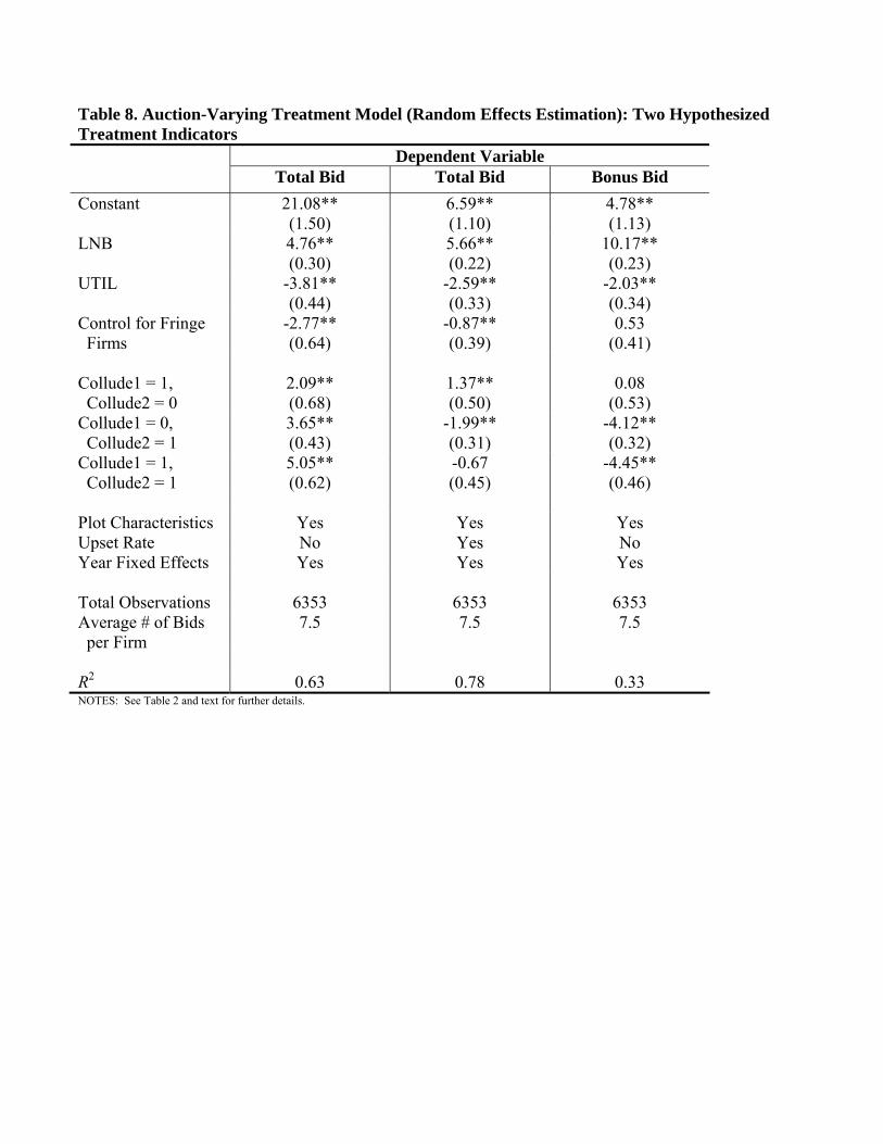
Table 8. Auction-Varying Treatment Model (Random Effects Estimation): Two Hypothesized Treatment Indicators Dependent Variable Total Bid Total Bid Bonus Bid Constant 21.08**

(1.50) 6.59** (1.10)

4.78** (1.13)

LNB 4.76** (0.30)

5.66** (0.22)

10.17** (0.23)

UTIL -3.81** (0.44)

-2.59** (0.33)

-2.03** (0.34)

Control for Fringe Firms

-2.77** (0.64)

-0.87** (0.39)

0.53 (0.41)

Collude1 = 1, Collude2 = 0

2.09** (0.68)

1.37** (0.50)

0.08 (0.53)

Collude1 = 0, Collude2 = 1

3.65** (0.43)

-1.99** (0.31)

-4.12** (0.32)

Collude1 = 1, Collude2 = 1

5.05** (0.62)

-0.67 (0.45)

-4.45** (0.46)

Plot Characteristics Yes Yes Yes Upset Rate No Yes No Year Fixed Effects Yes Yes Yes Total Observations 6353 6353 6353 Average # of Bids per Firm

7.5 7.5 7.5

R2 0.63 0.78 0.33 NOTES: See Table 2 and text for further details.

Table 9. Auction-Varying Treatment Model (Random Effects Estimation): Exchangeability Tests Sample All Bids

Non-Colluding

Bids Colluding

Bids Constant 22.986**

(1.438) 23.162** (1.608)

19.942** (3.144)

LSPI 0.275** (0.009)

0.277** (0.011)

0.282** (0.020)

DC -0.658** (0.059)

-0.706** (0.066)

-0.545** (0.130)

VPH 16.324** (1.183)

15.768** (1.297)

20.411** (2.945)

NCV 0.103** (0.021)

0.095** (0.024)

0.168** (0.047)

SLOPE -0.163** (0.017)

-0.156** (0.019)

-0.179** (0.037)

LNVPT 8.462** (0.325)

7.753** (0.375)

8.942** (0.646)

BWDN -7.610** (1.285)

-6.942** (1.415)

-12.862** (3.164)

BURN -20.316** (1.376)

-20.153** (1.406)

-45.255* (23.897)

CY -12.867** (0.854)

-12.861** (0.918)

-13.208** (2.746)

HP -43.804** (1.350)

-43.673** (1.392)

-69.830** (20.737)

HORSE -16.407** (0.749)

-16.155** (0.808)

-15.937** (1.909)

CYCLE -2.350** (0.084)

-2.351** (0.095)

-2.418** (0.176)

LNB 4.447** (0.265)

4.145** (0.304)

5.350** (0.571)

UTIL -1.770** (0.397)

-1.493** (0.462)

-3.094** (0.782)

Control for Fringe Firms -2.039** (0.517)

-1.806** (0.532)

-0.908 (4.110)

Year Fixed Effects Yes Yes Yes Total Observations 6353 4878 1475 Number of Firms 847 846 127 Average Bids per Firm 7.5 5.8 11.6 R2 0.620 0.616 0.631 Predicted Markup:

upsetux ˆˆ +β

2.953

3.313

1.754

H0: βnon-collude = βcollude

p=0.00

NOTES: Dependent variable is total bid. When the upset rate is included as a regressor, the p-value for the test of exchangeability is p=0.00. When the bonus bid is the dependent variable, the p-value is p=0.00 as well. See Table 2 for further details.

Table 10. Distribution-Based Treatment Model: Tests of Equality of Bid Distributions Unconditional Distributions

Adjusting for Covariates

Treatment Definition

deq p-value deq p-value I. Total Bid Collude = 1 (Auction-Invariant Indicator)

4.245 0.000 5.022 0.000

Collude1 = 1, Collude2 = 1 (Auction-Invariant Indicators)

3.665 0.000 4.018 0.000

Collude = 1 (Auction-Varying Indicator)

5.301 0.000 8.930 0.000

Collude1 = 1, Collude2 = 1 (Auction-Varying Indicators)

6.109 0.000 5.689 0.000

II. Total Bid Collude = 1 (Auction-Invariant Indicator)

4.245 0.000 5.772 0.000

Collude1 = 1, Collude2 = 1 (Auction-Invariant Indicators)

3.665 0.000 3.944 0.000

Collude = 1 (Auction-Varying Indicator)

5.301 0.000 7.556 0.000

Collude1 = 1, Collude2 = 1 (Auction-Varying Indicators)

6.109 0.000 5.361 0.000

III. Bonus Bid Collude = 1 (Auction-Invariant Indicator)

1.231 0.036 3.763 0.000

Collude1 = 1, Collude2 = 1 (Auction-Invariant Indicators)

0.946 0.394 2.665 0.000

Collude = 1 (Auction-Varying Indicator)

2.234 0.000 10.065 0.000

Collude1 = 1, Collude2 = 1 (Auction-Varying Indicators)

2.496 0.000 2.719 0.000

NOTES: Distributions are adjusted for covariates via inverse propensity score weighting, where the condition set is the same set of control variables as in Tables 2 – 8, where Panel I (II) does not (does) condition on the upset rate as well.