INFERRING PHYLOGENETICAL TREE BY USING HIERARCHICAL SELF ORGANIZING

MAPS

A THESIS

SUBMITTED TO THE DEPARTMENT OF COMPUTER

ENGINEERING

AND THE INSTITUTE OF ENGINEERING AND SCIENCE

OF BILKENT UNIVERSITY

IN PARTIAL FULFILLMENT OF THE REQUIREMENTS

FOR THE DEGREE OF

MASTER OF SCIENCE

By

Hayretdin Bahşi

January, 2002

I certify that I have read this thesis and that in my opinion it is fully adequate, in scope

and in quality, as a thesis for the degree of Master of Science

Assist. Prof. Dr. Atilla Gürsoy (Supervisor)

I certify that I have read this thesis and that in my opinion it is fully adequate, in scope

and in quality, as a thesis for the degree of Master of Science

Assist. Prof. Dr. Uğur Doğrusöz

I certify that I have read this thesis and that in my opinion it is fully adequate, in scope

and in quality, as a thesis for the degree of Master of Science

Assoc. Prof. Dr. Volkan Atalay

Approved for the Institute of Engineering and Science

Prof. Dr. Mehmet Baray

Director of the Institute of Engineering and Science

ABSTRACT

INFERRING PHYLOGENETICAL TREE BY USING HIERARCHICAL SELF ORGANIZING MAPS

Hayretdin Bahşi

M.S in Computer Engineering Supervisor: Assist. Prof. Dr. Atilla Gürsoy

Co-supervisor: Assist. Prof. Dr. Rengül Çetin Atalay January, 2002

In biology, inferring phylogenetical tree is an attempt to describe the

evolutionary history of today’s species with the aim of finding their common ancestors.

Specifically in molecular biology, it is used in understanding the evolution relationships

between proteins or DNA sequences. Inferring phylogenetical tree can be a very

complicated task since even for the input data having thirty sequences, the best tree

must be chosen among 1036 possible trees. In order to find the best one in a reasonable

time, various hierarchical clustering techniques exist in the literature. On the other side,

it is known that Self Organizing Maps (SOM) are very successful in mapping higher

dimensional inputs to two dimensional output spaces (maps) without having any priori

information about input patterns. In this study, SOM are used iteratively for tree

inference. Two different algorithms are proposed. First one is hierarchical top-down

SOM method which constructs the tree from the root to the leaves. Second one uses a

bottom-up approach that infers the tree from the leaves to the root. The efficiency of

Hierarchical SOM is tested in terms of tree topology. Hierarchical SOM gives better

results than the most popular phylogeny methods, UPGMA and Neighbor-joining. Also

this study covers possible solutions for branch length estimation problem.

Keywords: Phylogenetic Tree, Self Organizing Map, Kohonen Map, Evolution, DNA

ÖZET

HİYERARŞİK KENDİ KENDİNE ÖĞRENEN SİNİR AĞLARIYLA FİLOGENETİK AĞAÇ YAPISININ

OLUŞTURULMASI

Hayretdin Bahşi Bilgisayar Mühendisliği, Yüksek Lisans

Tez Yöneticileri: Yrd. Doç. Dr. Atilla Gürsoy, Yrd. Doç. Dr. Rengül Çetin Atalay

Ocak, 2002

Biyoloji alanında filogenetik ağaç yapıları, şu anda varolan türlerin ortak

atalarının belirlenerek bu türlerin evrimsel geçmişinin açıklanması amacıyla

oluşturulur. Özellikle moleküler biyoloji alanında, bu ağaç yapıları, proteinlerin veya

DNA dizilerinin evrimsel ilişkilerini ortaya çıkarmak için kullanılır. Çoğu zaman,

filogenetik ağaç yapılarının oluşturulması zor ve karmaşık bir işlem gerektirmektedir.

Örneğin, 30 DNA dizisine sahip bir girdi için 1036'dan fazla farklı ağaç yapısının

arasından en iyisini seçmek gerekir. En iyi olan ağaç yapısının uygun bir zaman içinde

belirlenebilmesi için literatürde bir çok hiyerarşik kümeleme teknikleri mevcuttur.

Diğer yandan, kendi kendine öğrenen sinir ağları, girdi türleri hakkında her hangi bir

bilgi sahibi olmadan çok boyutlu girdilerin iki boyutlu çıktı uzaylarına indirgenmesinde

çok başarılı olmaktadır. Bu çalışmada, kendi kendine öğrenen sinir ağları yöntemi ard

arda kullanılarak ağaç yapıları oluşturulmaktadır. Bu amaçla, iki farklı algoritma

tasarlanmıştır. Birincisi, ağacı kökten başlayıp yapraklara doğru giderek

oluşturmaktadır. İkincisi ise ağacı oluşturmaya yapraklardan başlamakta ve köke doğru

ilerlemektedir. Tasarlanan algoritmalar ağaç topolojisinin doğruluğu göz önüne alınarak

test edilmiştir. Bu algoritmalar, çok kullanılan UPGMA ve Komşu birleştirme

metotlarından çok daha iyi sonuç vermektedir. Ayrıca bu çalışma, ağaç kollarının

uzunluklarını tahmin etme problemi için de bazı çözümler sunmaktadır.

Anahtar Kelimeler: Filogenetik Ağaç Yapısı, Kendi Kendine Öğrenen Sinir Ağları, Evrim, DNA

ACKNOWLEDGEMENT I would like to express my deep gratitude to my supervisor Dr. Atilla Gürsoy and my

co-superviser Dr. Rengül Çetin Atalay for their guidance and suggestions throughout

the development of this thesis.

I would like to thank Dr. Uğur Doğrusöz and Dr. Volkan Atalay for accepting to read

and review this thesis.

I am grateful to my wife and my parents for supporting me during all the difficult times

of my study.

Contents

1. Introduction ..............................................................................................................1

2. Background on Phylogenetical Tree ........................................................................ 5

2.1 Input Data Types .............................................................................................. 5

2.1.1 Character-Based Data............................................................................... 5

2.1.2 Distance-Based Data ................................................................................ 7

2.2 Methods of Inferring Phylogenetical Tree ....................................................... 8

2.2.1 Distance-based Methods .......................................................................... 9

2.2.1.1 UPGMA(Unweighted Pair Group Method) and WPGMA (Weighted

Pair Group Method) ..........................................................................................12

2.2.1.2 Neighbor-Joining Method ..................................................................15

2.2.2 Maximum-Parsimony Methods..............................................................17

2.2.3 Optimal Tree Searching Algorithms ......................................................18

3. Background on Self Organizing Maps and Their Application to Phylogeny

Problem ..........................................................................................................................19

3.1 Overview of SOM Algorithm ........................................................................19

3.1.1 SOM Map...............................................................................................19

3.1.2 Unsupervised Learning .......................................................................... 20

3.1.3 Neighborhood and Learning Rate Functions ......................................... 21

3.2 Phylogeny Solutions with SOM..................................................................... 23

VII

4. Hierarchical SOM Algorithms ............................................................................... 26

4.1 Transformation of Character Data to Numeric Vectors ................................. 27

4.2 DNA Sequence Clustering with SOM ........................................................... 30

4.3 Hierarchical Top-down SOM Algorithm ....................................................... 32

4.4 Hierarchical Bottom-Up SOM Algorithm...................................................... 34

5. Evaluation of Hierarchical SOM Algorithms ........................................................ 39

5.1 Topology Testing Method.............................................................................. 39

5.2 Test Results of Hierarchical SOM Algorithms .............................................. 42

5.2.1 General Comparison............................................................................... 44

5.2.2 Fine-Tuning of SOM Parameters ........................................................... 46

6. Branch Length Estimation...................................................................................... 50

6.1 Branch Length Estimation Method s.............................................................. 50

6.1.1 Average Vector Method ......................................................................... 51

6.1.2 Weight Vector Method........................................................................... 52

6.1.3 Consensus Vector Method ..................................................................... 52

6.2 Test method for Branch Length Estimation Quality ...................................... 52

6.3 Comparison of Branch Calculation Methods ................................................. 53

6.4 Evaluation of Hierarchical SOM with Branch Error Estimation Method..... 54

7. Conclusion and Future Work ................................................................................. 55

8. Bibliography........................................................................................................... 57

9. Some Data Sets and Sample Inferred Trees ........................................................... 59

9.1 Tp53 ............................................................................................................... 59

9.2 Actin ............................................................................................................... 61

9.3 Globin............................................................................................................. 64

List Of Figures Figure 2-1. An example tree inferred from character data............................................... 6

Figure 2-2. An example tree inferred from distance data ................................................ 7

Figure 2-3. Inferred tree from ultrametric data ..............................................................10

Figure 2-4. Inferred tree from additive data...................................................................11

Figure 2-5. First step of tree inference with UPGMA....................................................14

Figure 2-6. Inferred tree after the second iteration of UPGMA.....................................15

Figure 2-7. Final inferred tree by UPGMA....................................................................15

Figure 2-8. Final inferred tree by Neighbor-joining method .........................................17

Figure 3-1. General structure of Self Organizing Maps................................................. 20

Figure 3-2. An example SOM map produced ................................................................ 24

Figure 3-3. One cycle training of SOTA...................................................................... 24

Figure 4-1. A sample transformation of character based input to numeric vector......... 30

Figure 4-2. Classification of DNA sequences with SOM map ...................................... 31

Figure 4-3. A sample trace of Hierarchic top-down SOM algorithm ............................ 34

Figure 4-4. A sample trace of Hierarchical Bottom-up SOM algorithm ....................... 37

Figure 4-5. The final tree inferred by Hierarchical Bottom-up SOM algorithm............ 38

Figure 5-1. A sample phylogenetical tree ...................................................................... 41

Figure 5-2. Phylogenetical tree of actin data inferred by Hieararchic Top-down SOM 43

Figure 5-3. Phylogenetical tree of actin data inferred by Neighbor-joining Method.... 43

Figure 5-4. Comparisons of test results according to topology testing method............. 45

Figure 5-5. Efficiency of methods for different size input vectors ............................... 46

Figure 6-1. A sample Phylogenetical tree ...................................................................... 51

List of Tables

Table 2-1. A Sample for Binary Character State Matrix.................................................. 6

Table 2-2. Distance data matrix example......................................................................... 7

Table 2-3. Ultrametric distance data ..............................................................................10

Table 2-4. Additive distance data...................................................................................11

Table 2-5 An example data matrix for UPGMA method...............................................13

Table 2-6. Data matrix at the end of first step of UPGMA............................................14

Table 4-1. Transition probabilities according to Jukes-Cantor model ........................... 27

Table 4-2. A sample nucleotide distance matrix for Jukes-Cantor model ..................... 28

Table 4-3. Transition probabilities according to ............................................................ 28

Table 4-4. A sample nucleotide distance ....................................................................... 29

Table 5-1. A sample distance data matrix ...................................................................... 41

Table 5-2. Test results of all data sets according to topology testing method ............... 44

Table 5-3. Test results of data sets having different sequence lengths .......................... 46

Table 5-4.Test results of Hierarchical bottom-up SOM for different initial learning rates

................................................................................................................................ 47

Table 6-1. Test results of all data sets with different ..................................................... 53

Chapter 1

1. Introduction The dominant view about the evolution of life is that all the existing organisms

are derived from common ancestors. New species are originated by splitting of

common ancestors into two or more populations with slow transformations in a very

long time. Therefore, evolution of life can be displayed by a tree which has a

common root and all other nodes are its descendents. In literature, such trees are

named as phylogenetical trees.

In biology, inferring phylogenetical tree is an attempt to describe the

evolutionary history of today’s species, populations or other taxonomical units [2].

But specifically in molecular biology, phylogenetical tree is used in understanding the

evolution relationships between proteins or DNA sequences. This study focuses on

trees of DNA sequences.

A tree is that tree is an undirected acyclic connected graph [3] which is

composed of exterior (leaves) and interior nodes. These nodes are connected to each

other by edges. In phylogenetical tree, leaves are species or taxonomical units

belonging to current time, interior nodes are ancestors of them and edges are the

evolutionary distances between nodes. Evolutionary distances can be interpreted as

the estimate of time that takes from evolution of one node from the ancestor node.

2

But generally this distance is not equivalent to elapsed time [2]. In a tree structure,

there is only one path between each pair of nodes [3]. The evolutionary distance

between any two nodes is the sum of edge lengths along this path.

Common problem of phylogenetical tree construction is determination of

whether phylogenetical tree has root or not. In most of the phylogeny problems,

determination of the root may not be available because of loss of data. In those cases,

inferred trees will be unrooted.

Generally two main aspects of phylogenetical trees are important. First one is

tree topology which is about how interior nodes are connected to leaves, and the

second one is the amount of evolutionary distances assigned to edges between pairs

of nodes.

There are two main types of input data for phylogenetical tree inferrence. One

of them is the distance matrix data which has all the pair wise evolutionary distances

of input sequences. The other one is the character state data matrix. In this matrix,

there are discrete characters for each input sequence and each character may have

different number of states. The aim in tree inferrence methods is finding the best tree

fitting to this input data. But the inferrence method must select the appropriate tree

among the huge number of possible ones. Even for 30 input sequences, the number

of possible unrooted trees is nearly 1036. Searching all of the trees and finding the best

one is an option, but it is impossible to reach the solution in a reasonable time for

data-sets having more than 20 sequences. In order to overcome this difficulty, two

main categories of inferring tree methods are decided. First category includes

clustering methods which use distance matrix data. These methods directly calculates

the optimum tree from the input data. But generally the inferred tree is not the best

one. The second type of methods use two major steps. First step is determination of

an optimality criteria (objective function) for evaluating the given tree. The second

step is computing the value of objective function with specific algorithms and finding

the best trees according to this criterion. The second method is usually slower than

the first one but yields better results.

This study tries to improve the performance of distance based methods in terms

of tree quality by using self organizing map which is a type of neural network. SOM

3

(Self Organizing Map) uses unsupervised learning method. It is a very powerful

clustering method and used in many areas of computational biology. Its strength

comes from having the ability of detecting second and higher order correlations in

patterns [8]. It can succesfully map high dimensional inputs to two dimensional

output spaces which are generally maps having predefined sizes. In inferring

phylogenetical tree problem, two main issues effect the quality of tree: Tree topology

and edge lengths which constitute evolutionary distances. If SOM is used in this

problem, it can give better quality tree topologies with the help of its clustering

strength. Since tree inference is not a simple clustering problem, SOM must be used

hierarchically.

In literature, there are some studies which use SOM in clustering proteins or

DNA sequences [8,13]. In these studies, SOM is just used only for clustering and

visualization purposes. SOM is also used for inferrence of phylogenetical tree (SOTA

[9]). But this study is not very sufficient in terms of proving the quality of its' results.

In this study, two different algorithms are constructed by using SOM

hierarchically. First one is the top-down approach which constructs the tree starting

from the root to the leaves and the second one is a bottom-up approach which infers

the tree from the leaves to the root. These methods propose solutions for

determination of tree topology.

In order to prove quality of inferred trees in terms of tree topology, a test

method is proposed. This method considers that all the edge lengths are unit

distances. It evaluates the inferred tree according to the distance matrix. Test results

are compared with the results of Neighbor-joining and UPGMA methods which are

the most famous distance based methods. Hierarchical SOM algorithms give better

results than Neighbor-joining and UPGMA algorithms. Then, the performance of

hieararchic SOM is fine tuned with adjusting the SOM parameters.

It is known that accurate estimation of branch lengths is the another important

factor in the quality of phylogenetical tree. This study also covers three different

intuitive solutions for this problem, average, weight and consensus vector methods.

These methods are compared with the results of Neighbor-joining and UPGMA by

using a method which estimates the error of inferred tree in terms of branch lengths.

4

But Neighbor-joining and UPGMA are better according to test results. More efforts

are needed for adaptation of Hierarchical SOM algorithm to branch length estimation

problem.

The following section, Chapter 2, provides detailed background information

about different phylogenetical tree inferrence methods that exist in literature. Chapter

3 focuses on SOM itself with SOM usage in protein clustering and inferring

phylogenetical tree problems. Chapter 4 gives details of Hierarchical SOM

algorithms. Then Chapter 5 presents tree topology testing method and discussion of

Hierarchical SOM test results. Chapter 6 describes some studies which are presented

for branch length estimation problem. Last chapter, Chapter 7 concludes overall

study.

Chapter 2

2. Background on Phylogenetical Tree This chapter includes an overview of phylogenetical tree inference methods. In

first part of this chapter, general information will be given about input data types for this

problem. This information is important because tree inference methods basically differ in

terms of input data. In other words, input data types show the logics under the methods.

After presentation of input data types, categories of tree inference methods will be

described.

2.1 Input Data Types Input data types can be classified into two main categories as character based and

distance based data.

2.1.1 Character-Based Data In this data type, each input objects (DNA sequences or proteins) have discrete

characters and each of the characters have a finite number of various states. The data

relative to these characters are placed in an objects * characters matrix, which we call

character state matrix. For example, in Table 2-1, there exists an example character

state matrix showing that whether each of five different objects A,B,C,D,E have the

properties C1, C2, C3, C4 and C5 or not. In this matrix, '0' means that corresponding

property does not exist in associated object. '1' says object has that property. If Table 2-

6

1 is observed carefully, it can be said that protein A has c3 and c4 properties but has no

others, protein B has c1 and c2 properties etc… The tree in Figure 2-1 is constructed

from the character state matrix in Table 2-1 (Details about creation of tree from the

given data is not important now).

In the inferred tree, similar objects are located in closer nodes. For example, objects 'B'

and 'D' have four common properties which mean they are highly similar to each other.

This similarity is reflected to tree topology so that they are sister nodes. Since 'E' has

different characters from B or D, they belong to disjoint sub-trees.

Figure 2-1. An example tree inferred from character data

Number of character states may change in various problems. For a sequence,

number of character states is 4 (A,T,G,C) for DNA and 21 for amino acids.

Objects C1 C2 C3 C4 C5 A 0 0 0 1 1 B 1 1 0 0 0 C 0 0 0 1 0 D 1 1 1 0 0 E 0 0 1 0 1

Table 2-1. A Sample for Binary Character State Matrix

EA C

B D

7

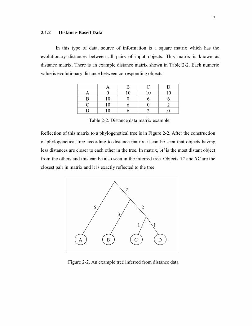
2.1.2 Distance-Based Data

In this type of data, source of information is a square matrix which has the

evolutionary distances between all pairs of input objects. This matrix is known as

distance matrix. There is an example distance matrix shown in Table 2-2. Each numeric

value is evolutionary distance between corresponding objects.

Reflection of this matrix to a phylogenetical tree is in Figure 2-2. After the construction

of phylogenetical tree according to distance matrix, it can be seen that objects having

less distances are closer to each other in the tree. In matrix, 'A' is the most distant object

from the others and this can be also seen in the inferred tree. Objects 'C' and 'D' are the

closest pair in matrix and it is exactly reflected to the tree.

Figure 2-2. An example tree inferred from distance data

A B C D A 0 10 10 10 B 10 0 6 6 C 10 6 0 2 D 10 6 2 0

Table 2-2. Distance data matrix example

1 1

2 3

2

5

A B C D

8

2.2 Methods of Inferring Phylogenetical Tree

Phylogenetical tree inference methods must overcome big difficulty, lack of

enough data about history. It predicts the historical ancestors of today's species, but

generally we don't have direct information about past [2]. Source information is

generally existing molecules or species. So, tree prediction is done by elimination of

tree candidates among the all possible trees with the limited knowledge and finding the

best one. The first solution that may come to mind can be exhaustive searching of all

possible trees. But two big problems arise at this stage. One of them is the huge amount

of possible tree combinations for even small number of input sequences. For example,

if there exist 10 input sequences, the number of possible trees exceeds two million. For

data sets having more than 20 sequences, finding the best tree in a reasonable time is

impossible. The second and more serious problem is how it can be determined that

whether one tree is better than the other. So, tree inference solutions firstly need to

present an optimality criterion (objective function) for the evaluation of any given tree.

The result of this evaluation is used to compare any tree with the others. Then, the

solution needs an algorithm for finding the best tree according to this objective

function. It must be pointed out that objective function is not used for only evaluation

of a tree. More or less (according to quality of objective function) it may help to shrink

the possible tree search space. So, some heuristic algorithms can be used from that

point. But, there exist another approach which combines the objective function and best

tree finding method into one complete algorithm. Rather than solving the problem in

two steps, it tries to reach to solution with just one step. Hierarchical clustering

techniques are widely used for this aim. This approach is faster than the first one but

tree quality can be lower. On the other side, first solution can still suffer from reaching

to the best tree in a reasonable time.

In the lights of previous descriptions, inferring tree algorithms can be

categorized into two broad types: Distance based methods and maximum-parsimony

methods. Distance-based methods use the input data which is the pair wise evolutionary

distances of all input sequences. The main goal is reflecting all these distances correctly

to a tree. These methods combine objective function and optimal tree finding algorithm

9

into one complete solution by using clustering techniques. On the other side,

maximum-pasimony methods take the approach of two steps solution. They do not

reduce biological datum to evolutionary distances, they use character-based data

directly [7]. The goal is building a tree structure in which input sequences are put to the

leaves of the tree and sequences of ancestor nodes are inferred so that the mutations

implied in the evaluation history is minimized. Objective function must be chosen in

order to minimize the mutations [2]. In the following two sections, more detailed

information about these methods will be given.

2.2.1 Distance-based Methods

Main differences of these methods with the others are that they use distance-

based data. These methods consider the problem in such a way that input sequences are

points in a euclidean vector space and all the pair wise distances between these points

are known. From that point, phylogeny problem is transformed into a clustering

problem. But in order to construct the tree structure, recursive clustering techniques are

used.

Basically, quality of inferred tree is related with two main issues in these types

of methods. First one is tree topology which is about how leaves are connected to

interior nodes. The second one is the quality of branch length estimations. So tree

inference methods must provide efficient solutions for both of these problems in order

to produce better results [2].

The properties of inferred trees are another important topics for distance-based

methods. Because final structural properties like being rooted or unrooted, are closely

related with these properties. There are two main types of tree properties, ultrametric

and additive property.

• Ultrametric Property

A tree has ultrametric property if the distances between any pairs of sequences

are equal to the total length of branches joining them and all of the sequences have the

same evolutionary distances from the root node.

10

Formal definition of ultrametric property is as follows:

Let D is the distance data matrix of sequence set and T is the rooted tree where

the leaves of the tree correspond to sequences. This tree is ultrametric if the following

conditions:

1. Each internal node of the tree is labeled by one distance from data matrix.

2. While going down from the root to leaves, the labeling numbering decreases.

3. For any sequence pair (i,j), D(i,j) is the label of least common ancestor of

sequences i and j. [1]

Suppose that there is a symmetric distance data matrix as shown in Table 2-3

A B C D E

A 0 8 8 5 3 B 8 0 3 8 8 C 8 3 0 8 8 D 5 8 8 0 5 E 3 8 8 5 0

Table 2-3. Ultrametric distance data

Tree (in Figure 2-3) can be inferred from this data as definition describes. It can be

realized that tree exactly reflects the input data matrix and each leaves have equal

distance from the root node.

Figure 2-3. Inferred tree from ultrametric data

3

3 5

8

A E

D B C

11

The key point of ultrametric property is that if an ultrametric tree can be

constructed from the given data, it means this tree is a perfect rooted phylogeny tree. In

other words, tree can be a rooted tree if it is ultrametric.

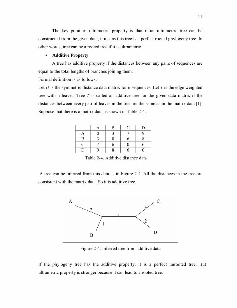
• Additive Property

A tree has additive property if the distances between any pairs of sequences are

equal to the total lengths of branches joining them.

Formal definition is as follows:

Let D is the symmetric distance data matrix for n sequences. Let T is the edge weighted

tree with n leaves. Tree T is called an additive tree for the given data matrix if the

distances between every pair of leaves in the tree are the same as in the matrix data [1].

Suppose that there is a matrix data as shown in Table 2-4.

A B C D A 0 3 7 9 B 3 0 6 8 C 7 6 0 6 D 9 8 6 0

Table 2-4. Additive distance data

A tree can be inferred from this data as in Figure 2-4. All the distances in the tree are

consistent with the matrix data. So it is additive tree.

Figure 2-4. Inferred tree from additive data

If the phylogeny tree has the additive property, it is a perfect unrooted tree. But

ultrametric property is stronger because it can lead to a rooted tree.

2

4

3

1

2

A

B

C

D

12

According to these tree properties, distance-based methods can be categorized.

Two different distance-based methods exist; UPGMA (or WPGMA) and neighbor-

joining.

2.2.1.1 UPGMA(Unweighted Pair Group Method) and WPGMA (Weighted Pair Group Method)

These are algorithms for inferring trees from ultrametric distance data. If data is

not ultrametric , data can not fit to a perfect tree and some errors will be occurred [2].

The general descriptions of these algorithms are as follows:

Input data is distance matrix of sequences. Let dij is the distance between

sequence ‘i’ and sequences ‘j’. First step is finding the pair of sequences with the

smallest distance. Then, these sequences are combined and they form a single new

sequence from that time. The distances of this new sequence (actually it is a cluster of

sequences) to others are calculated and they are added to data matrix. Also distance

data of old ones are erased Then again pair of sequences those having minimum

distance will be found. These merging processes continue until there remains one

cluster including all sequences. The steps of algorithm are as follows:

1. Each sequence is considered as a unique cluster.

2. From the distance matrix, find the clusters i and j such that dij is the

minimum value

3. Length of branch between i and j will be dij /2

4. If i and j were the last clusters then tree is completed otherwise create a

new cluster called u.

5. Distance from u to each other cluster k (k≠i or j) is the average value of

dki and dkj

6. Eliminate clusters i and j, add cluster u and return to step 2

Outline of clustering method is described above. But variations of these methods can be

implemented by changing the average function of step 5. The mostly common used

13

average function is the function which UPGMA algorithm uses. In this method, average

is calculated according to the number of sequences in the cluster. Suppose that cluster i

contains Ti sequences and cluster j contains Tj sequences. After merging of these two

clusters, new cluster u is created and distance between cluster u and any other cluster k

is calculated with Expression 2.1.

dku = (Ti dki + Tj dkj )/ (Ti + Tj ) (2.1)

At the averaging step, WPGMA (weighted pair group method) uses simple averaging

function (2.2).

dku = (dki + dkj )/ 2 (2.2)

Average function can be maximum (2.3) or minimum (2.4) value of two distances

dku = max(dki ,dkj ) (2.3)

dku = min(dki ,dkj ) (F6) (2.4)

If input data for clustering method is ultrametric, all of average functions infer the same

tree.

There is a sample of sequence data matrix in Table 2-5. This matrix includes the

distances of 5 rRNA sequences, Bsu, Bst, Lvi, Amo and Mlu.

Bsu Bst Lvi Amo Mlu Bsu 0 0.1715 0.2147 0.3091 0.2326 Bst 0 0.2991 0.3399 0.2058 Lvi 0 0.2795 0.3943

Amo 0 0.4289 Mlu 0

Table 2-5 An example data matrix for UPGMA method.

14

Let’s apply the UPGMA method to above data. At the first step, it can be realized that

the minimum distance is between Bsu and Bst. Then, these sequences form one cluster.

Inferring of tree is started as shown in Figure 2-5. Length of branch is calculated with

dividing the distance between Bsu and Bst by two. ( 0.1715/2=0.08575)

Figure 2-5. First step of tree inference with UPGMA

The next step is calculating the new data matrix. The new data matrix is in Table 2-6.

Distances between Bsu-Bst and other sequences are calculated with the Expression 2.1.

Table 2-6. Data matrix at the end of first step of UPGMA

The second clustering iteration again starts with finding the smallest distance which is

between Mlu and Bsu-Bst. At the end of this iteration, inferred tree is in Figure 2-6.

After all iterations, tree is completed. The complete tree is shown in Figure 2-7.

Bsu-Bst Lvi Amo Mlu Bsu-Bst 0 0.2569 0.3245 0.2192

Lvi 0 0.3399 0.3943 Amo 0 0.4289 Mlu 0

0.08575 0.08575

Bsu Bst

15

Figure 2-6. Inferred tree after the second iteration of UPGMA

Figure 2-7. Final inferred tree by UPGMA

2.2.1.2 Neighbor-Joining Method

This method infers additive tree. It uses basic clustering methodology of

UPGMA algorithm. The difference occurs in choosing of the clusters for the merging

process. Neighbor-joining does not only join the closest clusters, it combines the

clusters which are far from the rest. This method uses the minimum-evolution criteria

that can be calculated by Expression 2.5 [12].

0.08575

Bsu Bst Mluu

0.1096

Bsu Bst Mlu Lvi Amo

0.08575

0.1096

0.1398

0.1655

16

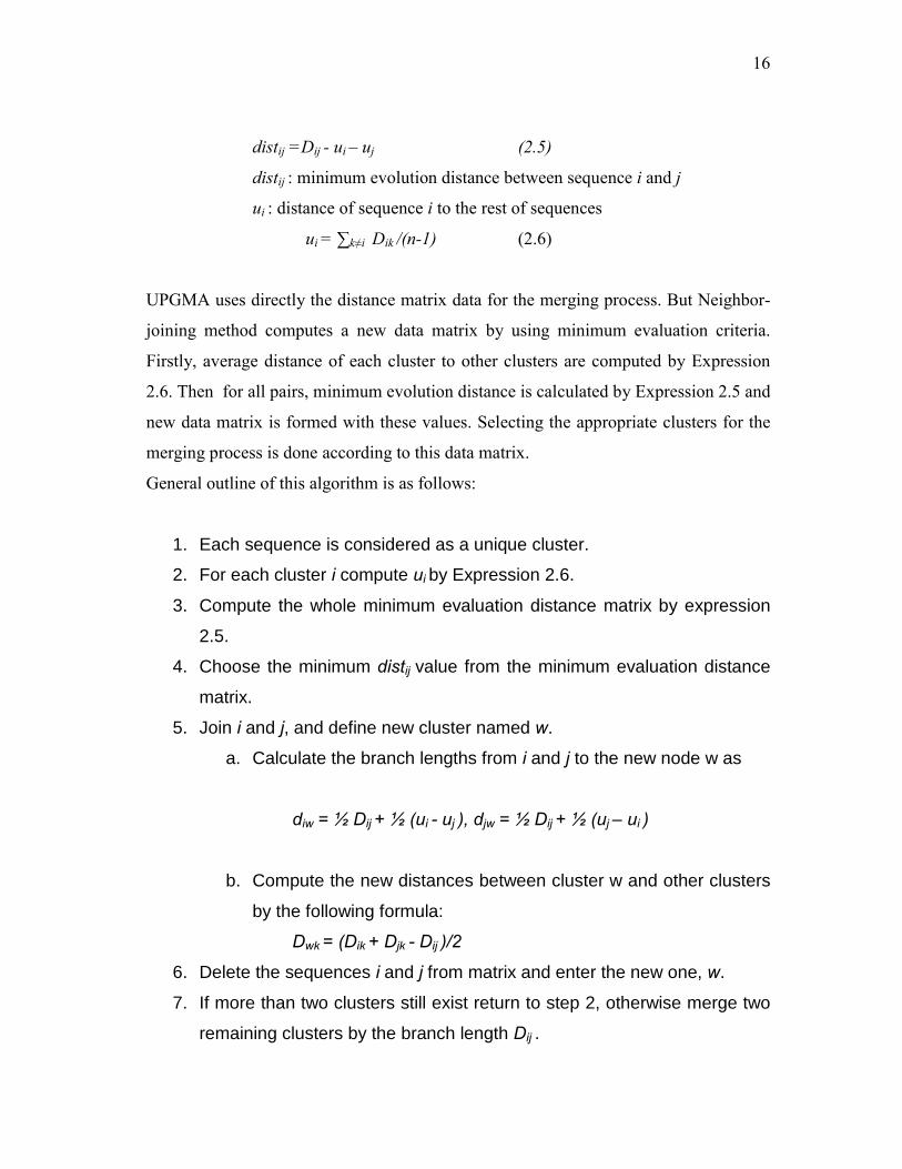
distij =Dij - ui – uj (2.5)

distij : minimum evolution distance between sequence i and j

ui : distance of sequence i to the rest of sequences

ui = ∑k≠i Dik /(n-1) (2.6)

UPGMA uses directly the distance matrix data for the merging process. But Neighbor-

joining method computes a new data matrix by using minimum evaluation criteria.

Firstly, average distance of each cluster to other clusters are computed by Expression

2.6. Then for all pairs, minimum evolution distance is calculated by Expression 2.5 and

new data matrix is formed with these values. Selecting the appropriate clusters for the

merging process is done according to this data matrix.

General outline of this algorithm is as follows:

1. Each sequence is considered as a unique cluster.

2. For each cluster i compute ui by Expression 2.6.

3. Compute the whole minimum evaluation distance matrix by expression

2.5.

4. Choose the minimum distij value from the minimum evaluation distance

matrix.

5. Join i and j, and define new cluster named w.

a. Calculate the branch lengths from i and j to the new node w as

diw = ½ Dij + ½ (ui - uj ), djw = ½ Dij + ½ (uj – ui )

b. Compute the new distances between cluster w and other clusters

by the following formula:

Dwk = (Dik + Djk - Dij )/2

6. Delete the sequences i and j from matrix and enter the new one, w.

7. If more than two clusters still exist return to step 2, otherwise merge two

remaining clusters by the branch length Dij .

17

Inferred tree with Neighbor-joining method for the example data set in Table 2-5 is

shown in Figure 2-8.

Figure 2-8. Final inferred tree by Neighbor-joining method

2.2.2 Maximum-Parsimony Methods

In science, parsimony means that simpler hypotheses are preferable to more

complicated ones. In computational biology, it is the name of mostly used method for

inferring tree from character-based data. These methods solve the tree inference

problem in two distinct steps. First step is defining an optimality criterion (objective

function) to compare different possible trees. The next step is finding trees those best

matches to the optimality criterion [2].

The main aim is finding the tree with the shortest total length. In these methods,

unit of length is evolutionary steps occurring during the transformation of one character

state to another. Steps can be base substitutions for nucleotide sequence data or gain,

loss events for restriction site data. There exist a common objective function for the

evaluation of any given tree. This function calculates total number of character state

changes along the all branches in the tree. In order to calculate total character state

changes, it traverses all branches of tree and assigns a cost value to each of them. Here,

cost is actually the number of character state changes that occurs along the tree branch.

Sum of all branch costs is total character changes. Optimal tree searching algorithms

evaluates all possible trees and finds the best tree with the minimal character changes.

0.0730.050

0.168

0.1110.0490.065

0.141

Bst Bsu Lvi

AmoMlu

18

2.2.3 Optimal Tree Searching Algorithms

Determining the optimal tree criterion and evaluating the existing tree

structure according to this criterion are different problems as stated before. Clustering

algorithms like UPGMA and Neighbor-joining methods solve the problem without

determining optimal tree criterion. The algorithms stated in this category solve the

problem of finding tree topology and predicting tree branch lengths according to the

predetermined criterion. They are mostly used with maximum-parsimony methods.

Finding the optimal tree is very expensive task in terms of needed

computational power because there exists huge number of possible trees even for small

number of inputs.

Chapter 3

3. Background on Self Organizing Maps and Their Application to Phylogeny Problem

This chapter gives general information about SOM algorithm and introduces

some phylogeny studies with SOM.

3.1 Overview of SOM Algorithm

Self Organizing Map [6] is a neural network type which uses unsupervised

learning method. Neural networks is very promising tool for application to many areas

of biology. They are able to detect second and higher order correlations in inputs [8].

They generate a mapping from high dimensional input space to lower dimensional

output usually to two dimensional systems which are called SOM maps. It reflects the

actual correlations of inputs to the map. Also training of this system does not need to

have a previous knowledge about the inputs.

3.1.1 SOM Map Basically, SOM map is an array of interconnected neurons (cells) as in Figure 3-1. All

cells in the input layer are connected to all cells in output layer. The spatial location of

20

a cell in the map corresponds to a specific region of the input space. Main aim is

providing that nearby inputs are categorized in the nearby map locations. In order to

supply this correlation between input space and output space, map is trained with a

training data set. For training, unsupervised competitive learning algorithm is used.

Figure 3-1. General structure of Self Organizing Maps

Each cell has a weight (reference) vector which is formed through the training process.

For each input, the euclidean distances between the weight vectors of each cell and the

input vector are calculated. The cell with the closest match of the input and its weight

vector produces an active output. In other words, each cell behaves like a pattern

detector for the same input and winning cell of the competition is the pattern that most

resembles to the input.

3.1.2 Unsupervised Learning

Formation of the weight vectors of cells occur through a training process.

Generally, training is done with a distinct training data set. Weight vectors are

initialized by random values or by input vectors drawn randomly from training data.

Each input from this set is presented to SOM system in order to calculate weight

Input Layer

Input

Output Layer

21

vectors. Winning cell for the each input is found. Then some of the cells are adapted

according to the input. Amount of adaptation and determination of cells that will be

adapted are the most important points of learning phase. Because these issues produce

the topological characteristic of the map. For example if only the weight vector of the

winning node is adapted, similar inputs are not placed in closer cells. In other words,

neighborhood property disappears. If all weight vectors are equally adapted, SOM map

could not accurately cluster the inputs. Special function which is known as

neighborhood function is used for choosing the cells which needs to adaptation. And

another function, learning rate function adjusts the amount of adaptation.

3.1.3 Neighborhood and Learning Rate Functions

According to neighborhood function, maximum adaptation will occur at the

winning node and neighborhood nodes of winning node are also updated. It has been

found experimentally that in order to achieve global ordering of the map, the

neighbourhood function firstly covers all of the cells to quickly produce a rough

mapping, but then it is reduced with time (here time means number of passes through

the training set data) to supply more localized adaptation of the map. Learning rate is

another factor in learning process which decreases with time. In order to achieve

quicker convergence of the algorithm, initially the learning rate should be high to

produce coarse clustering of nodes. As time passed, adaptation rate makes smaller

changes to weight vectors and local properties to the map are given.

Suppose that we want to train a SOM map which has K number of cells with

input vectors set {x | x∈ Rn}(n is the vector size). Each cell has a weight vector wk

(k=1,....,K). t is the time index and x(t) represents the input that is presented to SOM

system at time ’and wk(t) is the weight vector computed at time t.

The differences between input vector and weight vector is calculated with Euclidean

distance method for all weight vectors

dk(t) =|| x(t) - wk(t) ||, (k=1,...K) (3.1)

Suppose that c is the winning node, then winning node is found as:

22

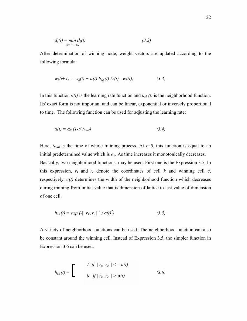
dc(t) = min dk(t) (3.2) (k=1,...,K) After determination of winning node, weight vectors are updated according to the

following formula:

wk(t+1) = wk(t) + α(t) hck (t) (x(t) - wk(t)) (3.3)

In this function α(t) is the learning rate function and hck (t) is the neighborhood function.

Its' exact form is not important and can be linear, exponential or inversely proportional

to time. The following function can be used for adjusting the learning rate:

α(t) = α0.(1-t/ ttotal) (3.4)

Here, ttotal is the time of whole training process. At t=0, this function is equal to an

initial predetermined value which is α0. As time increases it monotonically decreases.

Basically, two neighborhood functions may be used. First one is the Expression 3.5. In

this expression, rk and rc denote the coordinates of cell k and winning cell c,

respectively. σ(t) determines the width of the neighborhood function which decreases

during training from initial value that is dimension of lattice to last value of dimension

of one cell.

hck (t) = exp (-|| rk - rc ||2 / σ(t)2) (3.5)

A variety of neighborhood functions can be used. The neighborhood function can also

be constant around the winning cell. Instead of Expression 3.5, the simpler function in

Expression 3.6 can be used.

hck (t) = [ (3.6)

1 if || rk - rc || <= σ(t)

0 if|| rk - rc || > σ(t)

23

3.2 Phylogeny Solutions with SOM

Several studies have been made for different purposes in sequence analysis by

using neural network methods. Especially, they are used to classify biological

sequences but these neural network methods are based on supervised learning [15]. So

in these methods the classification knowledge of training set must be given which is

difficult to determine in large set of data. But in unsupervised methods, this priori

information is not needed and method itself categorizes the data. These methods can fit

to the needs of sequence analysis problem. Unsupervised neural network algorithms are

used in some studies for classification of protein sequences [8,13]. In these studies,

proteins are simply categorized with a predetermined size of SOM map. SOM is used in

the field of inferring phylogenetical tree by the study, named SOTA [9].

In SOM algorithm, map that is used for classification of data has certain

topology which is generally a grid like structure with two dimensions. But this structure

does not easily fit to a tree structure. SOTA solves this problem by using growing cell

structures algorithm of Fritzke [10] and a tree like structure for the map. Growing cell

structures algorithm simply divides the parts of map into much more components if the

number of inputs belonging that parts are bigger. An example is shown in Figure 3-2.

Suppose that we run SOM algorithm and get the distribution of inputs in SOM map as

in the left of the figure. Part a has much more elements so it is needed to divide into

much more components. At the next step that part is divided as shown in the figure.

Since other parts b, c and d have small number of inputs, they aren't needed to be

divided. SOTA combines this growing structure decision with tree-like structured map.

Initial structure is composed of one root and two terminal nodes. Each terminal node

behaves like a cell and has unique weight vector which is randomly initialized. Each

node also has a variable called local resource. It handles the heterogeneity of inputs

belonging to that node. If one input is assigned to a winning cell, the distance between

that input and weight vector is added to this variable. If a cell reaches to a heterogeneity

value more than the threshold, is divided into two descendent cells.

24

Figure 3-2. An example SOM map produced

by growing cell structures algorithm

Figure 3-3. One cycle training of SOTA

Suppose that we have five sequences as in Figure 3-3. Initial map is composed of one

root and two terminal nodes. During the training, winning node for sequences 1,3 and

4 is C1, and winning node for sequence 2 and 5 is C2. After determination of winning

nodes of each input, weight vector of corresponding node is updated as usual. But the

local resource variable is also computed. Consider the local resource variable of C1

a b

c d

Root

C1 C2

seq1 seq2 seq3 seq4 seq5

Root

C1 C2

Initial structure seq1 seq3 seq4

seq2 seq5

one cycle training

Sequences are categorized according to winning nodes

25

exceeds the threshold. Then two children of this node are created. At the end of the

training the whole tree structure is constructed and all weight vectors of nodes are

determined. This tree like map can be used for the categorization of inputs.

Since learning is adapted to tree structure directly, SOTA has problems with

the neighborhood condition. Global arrangements are done at the first stages in small

neighborhood area, some errors in these arrangements lead to totally wrong trees at the

end. This study doesn't provide comparative experimental results of real world data

with other methods to prove the efficiency of algorithm.

Chapter 4

4. Hierarchical SOM Algorithms

We proposed a new algorithm for inferring phylogenetical trees based on

hierarchical SOM maps. The first aim is adapting the conventional SOM approach to

inferring phylogenetical tree problem without destroying neighborhood and

unsupervised learning properties of SOM. Since output of SOM is a two dimensional

map, in this algorithm SOM maps are used hierarchically [18] in order to produce tree

structure. Input data for this algorithm is character-based data but it is converted to

numerical input vectors. Euclidean distances between these vectors are used in the

clustering process. So, it is an alternative method for distance-based methods presented

in Chapter 2.

Two different approaches of Hierarchical SOM method are presented in this study.

One of them uses top-down approach that constructs the tree from the root to the leaves

and the second one uses bottom-up approach that forms the tree in opposite direction,

from the leaves to the root. The details will be covered in the related sections. In this

chapter, firstly, transformation of character-based data to numerical vectors is

27

described. Then, detail of the SOM clustering technique is given. Finally, the

hierarchical SOM approach is presented.

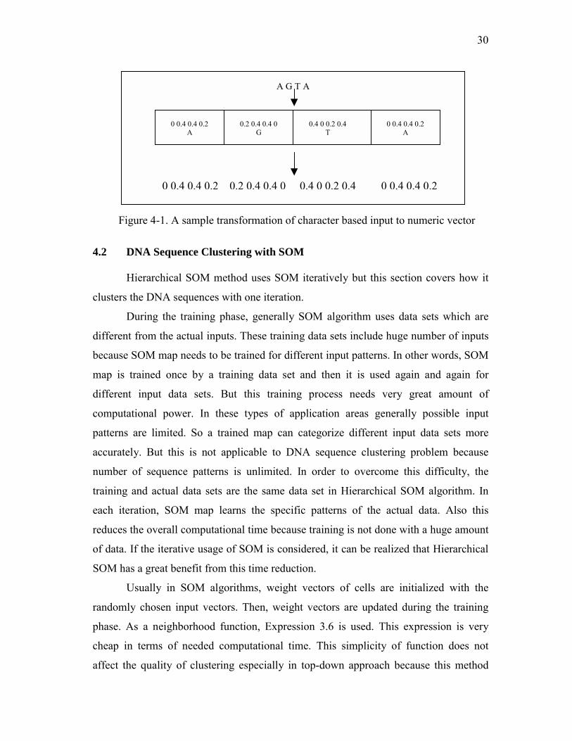
4.1 Transformation of Character Data to Numeric Vectors

DNA sequences are composed of four alphabet letters A, G, C, T and in biology

each of them is named as nucleotide. We want to represent each DNA sequence with a

vector such that Euclidean distance between the vectors of two DNA sequences are

proportional to their relativeness. First of all, the distances between each nucleotide

must be determined. To determine distances, help of nucleotide substitution models is

needed. Because, substitution rates between nucleotides may represent the similarities

between each other and these similarity definitions can be transformed into distance

values between sequences.

Substitution models define how and in which rate nucleotide substitutions

(mutations) may occur during the evolution. Jukes-Cantor model is the simplest one

and assumes that there is independent change at all sites (characters) with equal

probability [2]. According to this definition, substitution probabilities of nucleotides

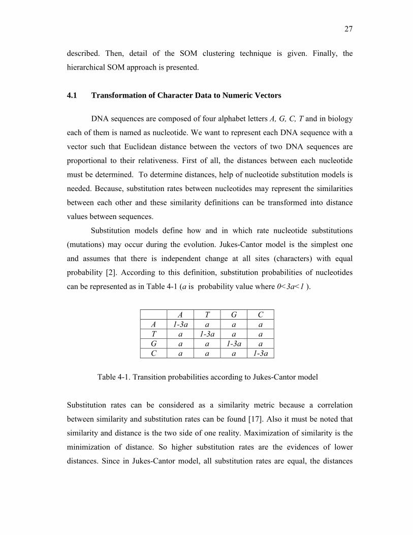
can be represented as in Table 4-1 (a is probability value where 0<3a<1 ).

A T G C A 1-3a a a a T a 1-3a a a G a a 1-3a a C a a a 1-3a

Table 4-1. Transition probabilities according to Jukes-Cantor model

Substitution rates can be considered as a similarity metric because a correlation

between similarity and substitution rates can be found [17]. Also it must be noted that

similarity and distance is the two side of one reality. Maximization of similarity is the

minimization of distance. So higher substitution rates are the evidences of lower

distances. Since in Jukes-Cantor model, all substitution rates are equal, the distances

28

between different nucleotides can also be considered as equal. So, matrix that is given

in Table 4.2 can be the distance matrix of nucleotides under Jukes-Cantor model.

Table 4-2. A sample nucleotide distance matrix for Jukes-Cantor model

Nucleotide bases fall into two categories depending on the ring structure of the

base. Purines (Adenine and Guanine) are two ring bases, pyrimidines (Cytosine and

Thymine) are single ring bases. A mutation that preserves the ring number is called a

transition (A <-> G or C <-> T ), a mutation that changes the ring number is called

transversion which occur between a purin and a pyrimidine (e.g. A <-> C or A <-> T).

The number of transitions observed in nature is much greater than the number of

transversions.

There is another substitution model called Kimura-2-parameter model [2]. This

is more complicated so that two different substitution rate values are used in this model.

Kimura-2-parameter model takes these transition and transversion rates into

consideration and presents a substitution model that is specified in Table 4-3.

A T C G

A 1-a-2b b b a

T b 1-a-2b a b

C b a 1-a-2b b

G a b b 1-a-2b

Table 4-3. Transition probabilities according to

Kimura-2-Parameter model

In this Table a represents the transition rate and b is the transversion rate. It is known

that transition rates are bigger than transversion rates. Since higher substitution rates

A T G C A 0 0.33 0.33 0.33 T 0.33 0 0.33 0.33 G 0.33 0.33 0 0.33 C 0.33 0.33 0.33 0

29

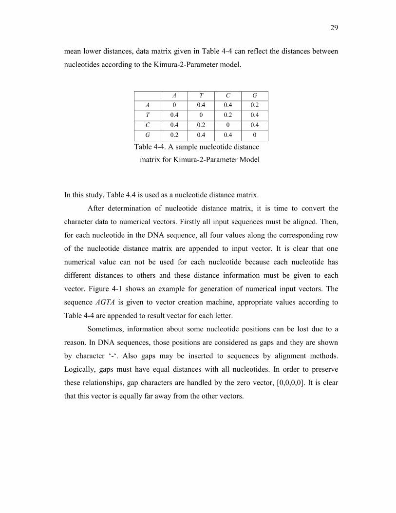
mean lower distances, data matrix given in Table 4-4 can reflect the distances between

nucleotides according to the Kimura-2-Parameter model.

Table 4-4. A sample nucleotide distance

matrix for Kimura-2-Parameter Model

In this study, Table 4.4 is used as a nucleotide distance matrix.

After determination of nucleotide distance matrix, it is time to convert the

character data to numerical vectors. Firstly all input sequences must be aligned. Then,

for each nucleotide in the DNA sequence, all four values along the corresponding row

of the nucleotide distance matrix are appended to input vector. It is clear that one

numerical value can not be used for each nucleotide because each nucleotide has

different distances to others and these distance information must be given to each

vector. Figure 4-1 shows an example for generation of numerical input vectors. The

sequence AGTA is given to vector creation machine, appropriate values according to

Table 4-4 are appended to result vector for each letter.

Sometimes, information about some nucleotide positions can be lost due to a

reason. In DNA sequences, those positions are considered as gaps and they are shown

by character ‘-‘. Also gaps may be inserted to sequences by alignment methods.

Logically, gaps must have equal distances with all nucleotides. In order to preserve

these relationships, gap characters are handled by the zero vector, [0,0,0,0]. It is clear

that this vector is equally far away from the other vectors.

A T C G A 0 0.4 0.4 0.2 T 0.4 0 0.2 0.4 C 0.4 0.2 0 0.4 G 0.2 0.4 0.4 0

30

Figure 4-1. A sample transformation of character based input to numeric vector

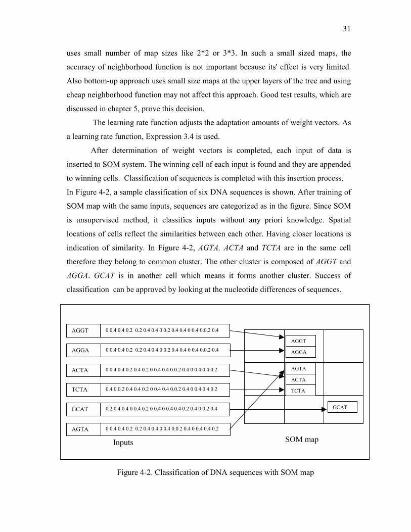
4.2 DNA Sequence Clustering with SOM Hierarchical SOM method uses SOM iteratively but this section covers how it

clusters the DNA sequences with one iteration.

During the training phase, generally SOM algorithm uses data sets which are

different from the actual inputs. These training data sets include huge number of inputs

because SOM map needs to be trained for different input patterns. In other words, SOM

map is trained once by a training data set and then it is used again and again for

different input data sets. But this training process needs very great amount of

computational power. In these types of application areas generally possible input

patterns are limited. So a trained map can categorize different input data sets more

accurately. But this is not applicable to DNA sequence clustering problem because

number of sequence patterns is unlimited. In order to overcome this difficulty, the

training and actual data sets are the same data set in Hierarchical SOM algorithm. In

each iteration, SOM map learns the specific patterns of the actual data. Also this

reduces the overall computational time because training is not done with a huge amount

of data. If the iterative usage of SOM is considered, it can be realized that Hierarchical

SOM has a great benefit from this time reduction.

Usually in SOM algorithms, weight vectors of cells are initialized with the

randomly chosen input vectors. Then, weight vectors are updated during the training

phase. As a neighborhood function, Expression 3.6 is used. This expression is very

cheap in terms of needed computational time. This simplicity of function does not

affect the quality of clustering especially in top-down approach because this method

0 0.4 0.4 0.2A

0.2 0.4 0.4 0G

0.4 0 0.2 0.4T

0 0.4 0.4 0.2A

A G T A

0 0.4 0.4 0.2 0.2 0.4 0.4 0 0.4 0 0.2 0.4 0 0.4 0.4 0.2

31

uses small number of map sizes like 2*2 or 3*3. In such a small sized maps, the

accuracy of neighborhood function is not important because its' effect is very limited.

Also bottom-up approach uses small size maps at the upper layers of the tree and using

cheap neighborhood function may not affect this approach. Good test results, which are

discussed in chapter 5, prove this decision.

The learning rate function adjusts the adaptation amounts of weight vectors. As

a learning rate function, Expression 3.4 is used.

After determination of weight vectors is completed, each input of data is

inserted to SOM system. The winning cell of each input is found and they are appended

to winning cells. Classification of sequences is completed with this insertion process.

In Figure 4-2, a sample classification of six DNA sequences is shown. After training of

SOM map with the same inputs, sequences are categorized as in the figure. Since SOM

is unsupervised method, it classifies inputs without any priori knowledge. Spatial

locations of cells reflect the similarities between each other. Having closer locations is

indication of similarity. In Figure 4-2, AGTA, ACTA and TCTA are in the same cell

therefore they belong to common cluster. The other cluster is composed of AGGT and

AGGA. GCAT is in another cell which means it forms another cluster. Success of

classification can be approved by looking at the nucleotide differences of sequences.

Figure 4-2. Classification of DNA sequences with SOM map

AGGT 0 0.4 0.4 0.2 0.2 0.4 0.4 0 0.2 0.4 0.4 0 0.4 0.0.2 0.4

ACTA 0 0.4 0.4 0.2 0.4 0.2 0 0.4 0.4 0.0.2 0.4 0 0.4 0.4 0.2

TCTA 0.4 0.0.2 0.4 0.4 0.2 0 0.4 0.4 0.0.2 0.4 0 0.4 0.4 0.2

GCAT 0.2 0.4 0.4 0 0.4 0.2 0 0.4 0 0.4 0.4 0.2 0.4 0.0.2 0.4

AGGT

AGGA

AGTA

ACTA

TCTA

GCAT

Inputs SOM map

AGGA 0 0.4 0.4 0.2 0.2 0.4 0.4 0 0.2 0.4 0.4 0 0.4 0.0.2 0.4

AGTA 0 0.4 0.4 0.2 0.2 0.4 0.4 0 0.4 0.0.2 0.4 0 0.4 0.4 0.2

32

4.3 Hierarchical Top-down SOM Algorithm

This algorithm iteratively uses SOM to construct the tree structure. It builds the

tree from the root to the leaves. Before the beginning of SOM iterations, the size of

map is determined. Initial structure of the tree is just only a root. In the first iteration,

all inputs are clustered with SOM. Each cell of the trained SOM map represents an

internal node in the tree and these internal nodes are descendants of root. In the next

iterations, these nodes will be the roots of the sub-trees which include the sequences of

the corresponding cells. If a cell has more sequences than a predetermined threshold

number, a new SOM iteration starts and sequences of this cell are clustered again. As in

the previous iteration, the cells of this map are children nodes. These iterations continue

until all cells have less number of sequences than the threshold number.

Let’s present this algorithm in a formal way. Suppose that Mk is the SOM map at

iteration k, K is the total number of maps created during the algorithm, the size of map

is x*y and Tk is the input set which SOM map Mk classifies. The number of elements of

set Tk is |Tk|. The set of sequences belonging to cell at (i,j) of Mk is Sk,i,j. |Sk,i,j| is the

number of sequences of this set. Pk is the root node of subtree which is formed by map

Mk. α is the threshold value for the number of sequences that is allowed to be in one

cell. The cells having less sequence number than α is not divided again. nm represents

the node which has a node index m and pm is the parent of this node.

There is an example in Figure 4-3. In this example hierarchic top-down

algorithm is applied to a sequence set which includes seven sequences. Threshold

number for the sequence number in the cell is equal to two. The initial tree is just a

root. The initial map S0 is created. Then S0 is trained with data and a,b,c,d,e,f and g are

clustered. The cells having two or less sequences are not processed more and they are

directly connected to the root. Since third partition has two sequences, one common

internal node is created and then they are directly connected to this node. S1 is formed

for the cell having four sequences and they are partitioned with this map. After this

iteration, there does not remain any cell which has number of sequences more than two.

Sequences are connected to node n1. For the cell having two sequences one more

internal node n3 is created.

33

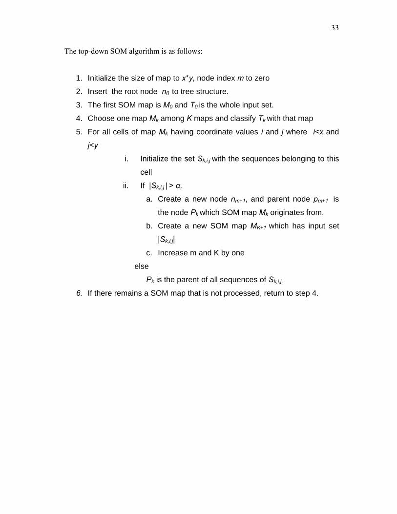
The top-down SOM algorithm is as follows:

1. Initialize the size of map to x*y, node index m to zero

2. Insert the root node n0 to tree structure.

3. The first SOM map is M0 and T0 is the whole input set.

4. Choose one map Mk among K maps and classify Tk with that map

5. For all cells of map Mk having coordinate values i and j where i<x and

j<y

i. Initialize the set Sk,i,j with the sequences belonging to this

cell

ii. If |Sk,i,j | > α,

a. Create a new node nm+1, and parent node pm+1 is

the node Pk which SOM map Mk originates from.

b. Create a new SOM map MK+1 which has input set

|Sk,i,j|

c. Increase m and K by one

else

Pk is the parent of all sequences of Sk,i,j.

6. If there remains a SOM map that is not processed, return to step 4.

34

Figure 4-3. A sample trace of Hierarchic top-down SOM algorithm

4.4 Hierarchical Bottom-Up SOM Algorithm

This method constructs the tree by starting from the leaves to the root. SOM

map has not a predetermined size, the algorithm itself chooses the size according to

number of inputs. At each iteration, the map size is recomputed. First iteration starts

with a large map size which can be nearly equal to input numbers. After classification,

for each cell of the map, an internal node is created and the sequences belonging to this

cell are connected to this internal node. By this way, the parents of leaves are found.

But tree structure must grow in upper direction and end with the root. At the end of

each SOM iteration, tree grows one upper layer towards the root. In the second

a b

c de

fg

n0

n0

n1 e n2

f g

a b

c

d

Initial tree with just only a root

S0

S1

n0

n1 e n2

f ga n3 b

c d

Tree after S0

Tree after S1

35

iteration, last created internal nodes must be classified in order to find their parent

nodes. So, internal nodes are categorized by a new created SOM map. But there arises a

problem in this stage that which vectors can represent the internal nodes during the

SOM classification. Weight vectors of cells in the previous SOM map can be good

representatives for the vectors of nodes. Since each cell is represented by a different

node in the structure, weight vectors of the previous map can be input vectors for the

map of the second iteration. But the size of the map must be changed because the input

number, which is actually equal to size of the previous map, is less than the number of

sequences. The new map size is computed by dividing the last map size by four. At the

end of the second iteration, we get closer to root by one more layer. These iterations

continue until the root is found. The overall algorithm of bottom-up approach is as

follows:

In this algorithm, Mk is the SOM map at iteration k, K is the total number of

maps created during the algorithm, the size of map is xk*yk and Tk is the input set which

SOM map Mk classifies. The number of elements of set Tk is |Tk|. The set of sequences

belonging to cell at (i,j) of Mk is Sk,i,j which has |Sk,i,j| number of sequences. nm

represents the node which has a node index m and pm is the parent of this node. N is the

number of al input sequences.

1. Initialize the map size x0*y0 so that x0* y0 ≈N. Node index m and K are

equal to zero.

2. The first SOM map is M0 and T0 is the whole input set.

3. Choose one map Mk among K maps and classify Tk with that map

4. For all map cells, Mk, having coordinate values i and j where i<x and j<y

i. Initialize the set Sk,i,j with the sequences belonging to this cell

ii. Add new internal node nm+1 and connect all the nodes in set

Sk,i,j to this internal node

iii. Increment m by one

5. If root is not still reached,

i. Create new map MK+1 . Input set, TK+1, is weight vectors of Mk

ii. New map sizes xK+1, yK+1 are the halves of previous ones,

ıncrement K by one and return to step 2.

36

Hierarchical bottom-up approach is described with an example in Figure 4.4. Input data

includes 10 sequences, a,b,c…i,j in this example. After the first iteration sequences are

clustered with SOM map S0. Each cell having at least one sequence forms a new node.

Part of the tree that is constructed at the end of the first iteration is shown in the figure.

In the second hierarchic iteration, weight vectors of S0 are the input data for map S1. S1 clusters these weight vectors and each cells of this map become new nodes. But there is

a difference at the size of SOM map. Length and width of map are the halves of the

previous ones. The tree at the end of this second iteration is shown in the left part of

SOM map S1. Tree is not completed yet. One more iteration is needed. After this

iteration, there is no need to continue. Because at the top level there are two nodes and

Connecting them by a root node completes the inferring tree process. The overall result

tree is shown in Figure 4-5. Some internal nodes have only one daughter node. So

internal nodes having one daughter cell may be erased in the tree structure.

37

Figure 4-4. A sample trace of Hierarchical Bottom-up SOM algorithm

a bc

de

f

g

hi

j

S0

0 1 2 3

0 1 2 3

0,0 0,2 1,3 2,1 3,03,3

ab

cf g

c e

i h i

0,0

2,1

3,0

0,2

1,3

3,3

4 5

4

5 0,0 0,2 1,3 2,1 3,33,0

4,4 4,5 5,4 5,5

4,5

4,4 5,4

5,5

6

6 7

4,4 4,5 5,4 5,5

6,6 6,7

Actual inputs

S1

S2

Weight Vectors of S0

Weight Vectors of S1

Second hierarchic iteration

Third hierarchic iteration

First hierarchic iteration

38

Figure 4-5. The final tree inferred by Hierarchical Bottom-up SOM algorithm

0,0 0,2 1,3 2,1

a b

c f g

c e

3,3

i

3,0

h i

4,4 4,5 5,4 5,5

6,6 6,7

Root

Chapter 5

5. Evaluation of Hierarchical SOM Algorithms

The quality of inferred tree depends on two main factors, good estimation of tree

topology and accuracy of branch length prediction, as stated before. So, these issues may

be the guidelines for the evaluations of phylogenetical tree inference methods.

This chapter focuses on evaluation of tree quality with respect to tree topology.

Firstly, a topology testing method is proposed. According to this method, general

comparison of each Hierarchical SOM algorithm with distance based methods, Neighbor-

joining and UPGMA, are done. In the last part, different test results of fine tuning efforts

for SOM parameters will be described.

5.1 Topology Testing Method

In this method, the main purpose is evaluation of the first factor of the

phylogenetical tree quality, tree topology. Tree topology means how nodes are

connected to each other. In a good tree, nodes must be connected to other nodes in such

a way that similar sequences reside in the same sub-trees. For example, in a well

40

inferred tree, the most similar ones must be descendants of a common node. In other

words, the distances between sequences must be proportionally reflected to tree in

terms of branch numbers. In this testing method, it is considered that each branch

length is equal to a unit distance, because the aim is just testing the branch orders.

Method starts with the computing of distance matrix that includes Euclidean distances

between all pairs of sequences (Suppose that S is the sequence data set). Then any two

distances are chosen from this matrix. Let's say one of the distances is between

sequences Si and Sj and the other one is between Sm and Sn. On the other side, these

sequences are represented by leaf nodes in the inferred tree. Suppose that sequences Si,

Sj, Sm and Sn are represented by nodes ni, nj, nm and nn in the tree and |ninj| is the tree

distance between nodes ni and nj. Since, branch lengths are unit distance, this tree

distance is actually the number of branches between these two nodes. If tree is perfectly

inferred, one of the following statements must be true('=>' represents if statement):

(|Si Sj| > |Sm Sn| ) => (|ninj|>|nmnn| )

or (5.1)

((|Sm Sn| >= |Si Sj| ) => (|nmnn|>|ninj| )

Expression (5.1) states that if one distance is bigger than the other one in actual data,

this must be preserved in the inferred tree in terms of branch numbers. This evaluation

is done for the all pairs of the distances in the distance matrix. A score value is used to

represent the quality of tree numerically. This value is initialized to zero at the

beginning, For each pair of distances, Expression 5.1 is evaluated, if one of the

statements is true, score value is increased by one. If perfect phylogenetical tree is

possible for the given data set and it is inferred exactly, score reaches to the maximum

value. According to this test, higher score values mean better trees. There is an example

data matrix in Table 5-1.

41

Table 5-1. A sample distance data matrix

The tree that is inferred from this data is shown in Figure 5-1. Let's trace topology testing

method in this example. Suppose that two distances from table are chosen, one of them is

11 which is between sequences S1 and S3, the other one is 21 which is between S2 and S4.

The tree distances of first pair can be calculated from the tree as 12 and the tree distance

of second pair is 23. Since (|S2S4|=21 > |S1S3| =11) and (|n2n4|=23 > |S1S3| =11) score value

is increased by one.

Figure 5-1. A sample phylogenetical tree

S1 S2 S3 S4 S5 S1 0 14 11 13 20 S2 14 0 12 21 23 S3 11 12 0 20 21 S4 13 21 20 0 11 S5 20 23 21 11 0

Inferred Tree

R

S1 N2

N1 N3

S4 S5

3 3

S2 S3

45

6 5

5 5

42

5.2 Test Results of Hierarchical SOM Algorithms

Hierarchical SOM algorithms are tested by seven different real world data sets,

tp53, actin, globin, hemoglobin, keratin, HBV and myosin. The number of sequences in

these data sets are 10, 14, 20, 34, 59, 100 and 200, respectively. They are prepared from

the gene databases which are available in the internet [11]. Number of sequences

change from ten to two hundred to show the efficiency of algorithms in different data

sizes. Each sequence has 70 nucleotides. But there are three additional keratin and HBV

data sets. They have nucleotide sizes with 140, 210 and 280. All input data sets are

aligned. Hierarchical SOM algorithms are evaluated with them to see the effect of

nucleotide size in the tree quality. Evaluation is done according to topology testing

method. Since these algorithms fall into the distance based category, they are compared

with Neighbor-joining and UPGMA methods. During this comparison, the outputs of

PHYLIP program package are used in which Neighbor-joining and UPGMA methods

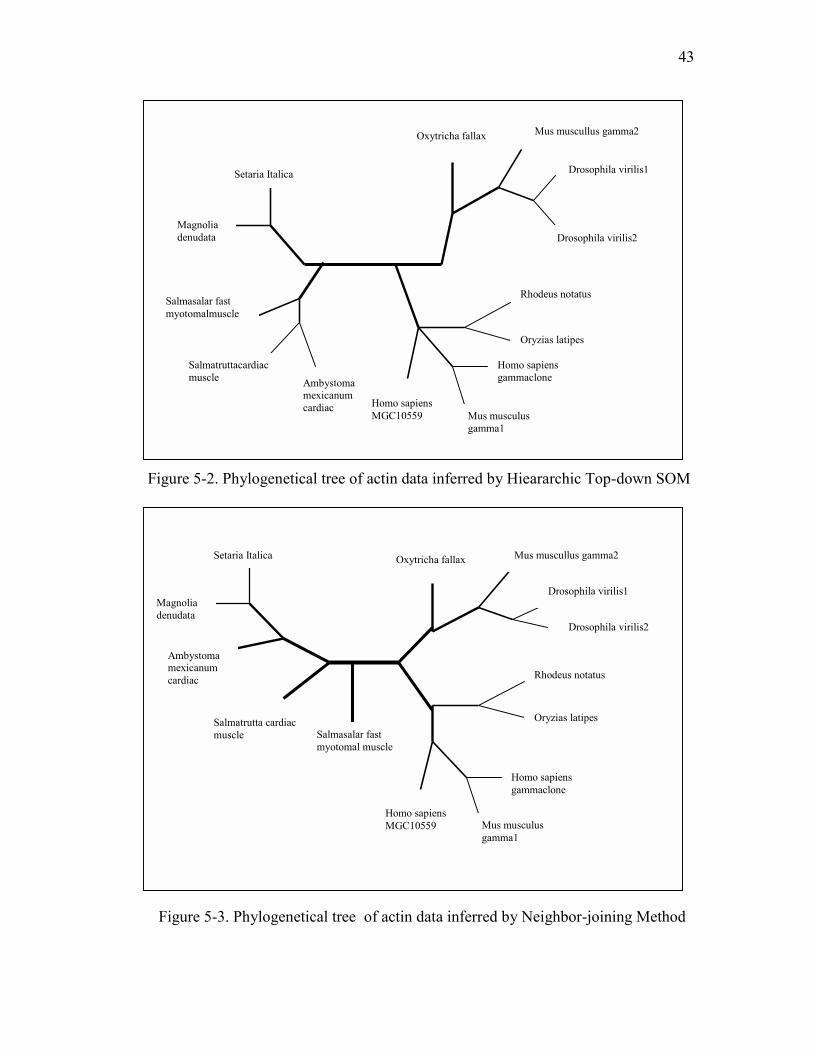
are implemented [5]. Let’s observe the inferred tree of actin data by Hierarchical SOM

top-down algorithm (shown in Figure 5-2). Map size is 2*2 in each hierarchical

iteration. Figure 5-3 is the inferred tree by Neighbor-joining program of PHYLIP. If

these two trees are compared, it can be seen that similarities of sequences are reflected

in both of the trees nearly in the same way. This observation is important so that it

gives initial intuition about efficiency of Hierarchical SOM algorithms. In most of the

big phylogeny data, important issue is finding the most similar sequences in such a

huge data. Most similar sequences must be sister nodes of each others in a good tree.

For example Drosophila_virilus1 and Drosophila_virilus2 are the daughter nodes of

common parent in both of the trees. This condition is hold for (Rhodeus_notatus,

Orvzias_latipes), (Sateria_italica, Magnolia_denudata) and (Homo sapiens gamma

1clone MGC,Mus musculusgamma1) pairs. So, in Hierarchical SOM, accurate

representations of similar sequences are at least as better as in Neighbor-joining

method. But this observation is not an exact comparison. So, it is time to apply

topology testing method.

43

Figure 5-2. Phylogenetical tree of actin data inferred by Hieararchic Top-down SOM

Figure 5-3. Phylogenetical tree of actin data inferred by Neighbor-joining Method

Oxytricha fallax Mus muscullus gamma2

Drosophila virilis1

Drosophila virilis2

Setaria Italica

Magnolia denudata

Salmasalar fast myotomal muscle

Salmatrutta cardiac muscle

Ambystoma mexicanum cardiac Rhodeus notatus

Homo sapiens MGC10559

Homo sapiens gammaclone

Mus musculus gamma1

Oryzias latipes

Rhodeus notatus Salmasalar fast myotomalmuscle

Salmatruttacardiac muscle Ambystoma

mexicanum cardiac

Oxytricha fallax Mus muscullus gamma2

Drosophila virilis1

Drosophila virilis2

Setaria Italica

Magnolia denudata

Homo sapiens MGC10559

Homo sapiens gammaclone

Mus musculus gamma1

Oryzias latipes

44

5.2.1 General Comparison Under this topic, hierarchical top-down, hierarchical bottom-up, Neighbor-

joining and UPGMA algorithms are evaluated. Since the size of map can be changed in

hierarchical top-down method, it is evaluated under various sizes of maps, 2*1, 2*2,

3*2 and 3*3. Table 5-2 includes the topology testing results. (Figure 5-4 shows the

ratio of test results to the Neighbor-joining throughput.)

Table 5-2. Test results of all data sets according to topology testing method

In this table, first column includes the names of data sets and second one represents the

number of sequences for each data. Results show that top-down 2*2 Hierarchical SOM

method yields better tree topologies for smaller data sets like actin and globin. But as

the number of sequences increase, the effectiveness of bottom-up approach also

increases. For large data sets like Keratin, HBV and Myosin, bottom-up approach is the

best method. The difference between the scores of bottom-up approach and the other

methods has the maximum value in the biggest data set, myosin. Bottom-up approach

classifies with large sized map at the first time, so SOM algorithm can reflect its

learning strength to the results of big data sets. Top-down methods classify with smaller

maps like 2*2, 3*2 or 3*3. These map sizes may not be enough to classify the large

data sets accurately but it is shown that they are sufficient in small ones. After the first

test, it can be concluded that Hierarchical SOM methods produce better tree topologies

than the conventional ones, UPGMA and Neighbor-joining.

Data sets Sequence Number

Top-down 2x1

Top-down 2x2

Top-down 3x2

Top-down 3x3

Bottom-up

UPGMA Neighbor Joining

Tp53 10 294 284 305 285 243 250 256 Actin 14 857 965 778 840 874 923 920

Globin 20 2497 2717 2693 2549 2421 2497 2590 Hemoglobin 34 11992 12244 13452 16435 13821 13060 13164

Keratin 59 59568 60405 69197 66649 77099 64388 64952

HBV 100 285796 307528 326595 337329 381506 301456 308851

Myosin 200 2386227 2363649 2429567 2625292 3259348 2393527 2392727

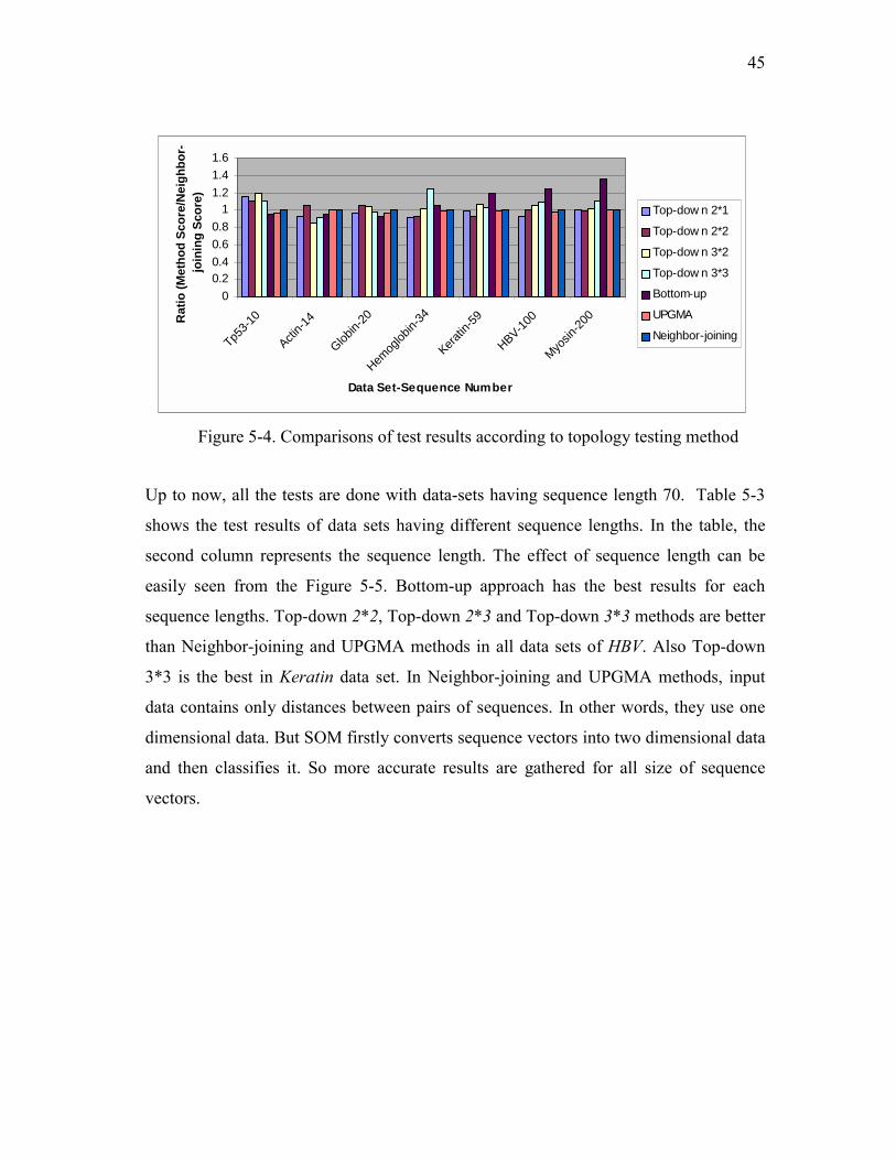
45

00.20.40.60.8

11.21.41.6

Tp53-1

0

Actin-1

4

Globin-

20

Hemog

lobin-

34

Keratin

-59

HBV-100

Myosin

-200

Data Set-Sequence Number

Rat

io (M

etho

d Sc

ore/

Nei

ghbo

r-jo

inin

g Sc

ore)

Top-dow n 2*1

Top-dow n 2*2

Top-dow n 3*2

Top-dow n 3*3

Bottom-up

UPGMA

Neighbor-joining

Figure 5-4. Comparisons of test results according to topology testing method

Up to now, all the tests are done with data-sets having sequence length 70. Table 5-3

shows the test results of data sets having different sequence lengths. In the table, the

second column represents the sequence length. The effect of sequence length can be

easily seen from the Figure 5-5. Bottom-up approach has the best results for each

sequence lengths. Top-down 2*2, Top-down 2*3 and Top-down 3*3 methods are better

than Neighbor-joining and UPGMA methods in all data sets of HBV. Also Top-down

3*3 is the best in Keratin data set. In Neighbor-joining and UPGMA methods, input

data contains only distances between pairs of sequences. In other words, they use one

dimensional data. But SOM firstly converts sequence vectors into two dimensional data

and then classifies it. So more accurate results are gathered for all size of sequence

vectors.

46

Data sets and sequence lengths

Top-down 2x1

Top-down 2x2

Top-down 3x2

Top-down 3x3

Bottom-up

Neighbor-joining

HBV-280 276330 290324 314876 330392 395045 295364 HBV-210 282936 317475 329673 328456 382355 295409 HBV-140 301504 301890 310291 336583 385601 296870 HBV-70 284349 305283 325920 336789 380456 307330 Keratin-280 55178 60612 60522 67273 77031 64525 Keratin-210 61111 62511 65169 61235 77725 66543 Keratin-140 63454 65644 62598 69398 74339 66003 Keratin-70 59568 60405 69197 66649 77099 64952

Table 5-3. Test results of data sets having different sequence lengths

0

50000

100000

150000

200000

250000

300000

350000

400000

450000

HBV-280 HBV-210 HBV-140 HBV-70 Keratin-280

Keratin-210

Keratin-140

Keratin-70

Data Sets and Sequence Lengths

Scor

e

Top-down 2x1Top-down 2x2Top-down 3x2Top-down 3x3Bottom-upNeighbor-joining

Figure 5-5. Efficiency of methods for different size input vectors

5.2.2 Fine-Tuning of SOM Parameters

As stated in section 3.1, accuracy of learning depends on two functions, learning

rate and neighborhood functions in SOM algorithms.

Learning rate function adjusts the adaptation amount of weight vectors so that

they are heavily updated at the beginning of the training to have a rough map. In the

later times, they are updated in small amounts to give detailed localization properties.

In Hierarchical SOM, Expression 3.4 is used as a learning function. Since the initial

47

value is a predetermined value, Hierarchical SOM algorithms are tested by different

initial learning rate values. Table 5-4 and Table 5-5 show the experimental test results

of Hierarchical bottom-up and top-down SOM methods with different initial learning

rate values. From Table 5-4, it can be concluded that all data sets except tp53, give the

best results with the initial learning rate values 0.75 or 0.9. But in Table 5-5, the best

results are reached by the value range between 0.45 and 0.55. Bottom-up approach

uses large map sizes. In these map sizes, classification accuracy much more depends on

learning so it gives best throughput in higher values of learning rate.

Data-sets Input number

0.1 0.3 0.6 0.75 0.9

Tp53 10 268 260 286 250 243 Actin 14 823 824 811 856 874

Globin 20 2200 2020 2170 2130 2421 Hemoglobin 34 12779 14043 14220 14252 13821

Keratin 59 63544 72556 76160 76475 77099 HBV 100 339175 391760 381514 394320 381506

Table 5-4.Test results of Hierarchical bottom-up SOM for different initial learning rates

Data-Sets Input

number 0.1 0.3 0.45 0.50 0.55 0.6 0.9

Tp53 10 315 343 348 338 338 338 284 Actin 14 957 970 965 965 965 970 965 Globin 20 2530 2726 2752 2752 2773 2650 2717 Hemoglobin 34 13139 13611 13932 13582 13463 13447 12244 Keratin 59 61781 62094 64661 61828 60555 61509 60405 HBV 100 321499 319115 329477 333450 344865 333413 307528Table 5-5. Test results of Hierarchical top-down SOM for different initial learning rates

The other function that needs to be adjusted is neighborhood function. Let's revisit the

Expression 3.6 again,

hck (t) = [

1 if || rk - rc || <= σ(t)

0 if|| rk - rc || > σ(t)

48

In this function, c is the winning neuron for the training input that is presented to SOM

system in time t. It must be decided whether weight vector of node k will be updated at

this time. || rk - rc || represents the Euclidean distance between the coordinates of

neurons k and c. s(t) is the width of the neighborhood function which is initially equal

to the size of all map and gradually decreases during training. Neighborhood function

hck(t) returns one or zero. If it returns one, this means neuron k will be updated. Zero

value concludes that neuron won't be updated at time t. Initialization of width value

may be done by lower values than the actual map size in order to have highly localized

map. For this aim, we add a weight value w to the expression as follows:

hck (t) = [

The weight value must be lower than one. Because the width of neighborhood function

must be strictly lower than the size of map. Table 5-6 and Table 5-7 show some

experimental results of Hierarchical bottom-up and top-down SOM methods with

different neighborhood width values. Initial learning rates are constant in all tests.

Data-sets Input number

0.2 0.5 0.7 0.8 1.0

Tp53 10 301 259 266 281 243 Actin 14 992 786 827 839 874 Globin 20 2029 2053 2319 2348 2421 Hemoglobin 34 11278 12549 12562 12496 13821 Keratin 59 72293 73850 70463 75519 77099 HBV 100 356653 364400 379296 382620 381506

Table 5-6. Test results of Hierarchical bottom-up SOM method

for different initial neighborhood widths

1 if || rk - rc || <= w.σ(t)

0 if|| rk - rc || > w.σ(t)

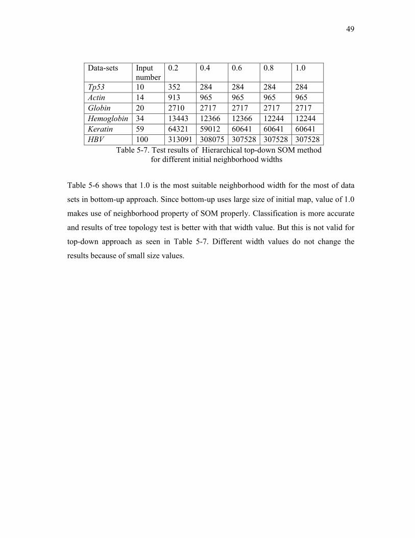
49

Data-sets Input number

0.2 0.4 0.6 0.8 1.0

Tp53 10 352 284 284 284 284 Actin 14 913 965 965 965 965 Globin 20 2710 2717 2717 2717 2717 Hemoglobin 34 13443 12366 12366 12244 12244 Keratin 59 64321 59012 60641 60641 60641 HBV 100 313091 308075 307528 307528 307528

Table 5-7. Test results of Hierarchical top-down SOM method for different initial neighborhood widths Table 5-6 shows that 1.0 is the most suitable neighborhood width for the most of data

sets in bottom-up approach. Since bottom-up uses large size of initial map, value of 1.0

makes use of neighborhood property of SOM properly. Classification is more accurate

and results of tree topology test is better with that width value. But this is not valid for

top-down approach as seen in Table 5-7. Different width values do not change the

results because of small size values.

Chapter 6

6. Branch Length Estimation

In top-down and bottom up SOM algorithms, the main aim was producing tree

topology with higher quality. But there is another important issue of phylogenetical tree

inference problem which is the calculation of branch lengths. Up to now, this problem

is not handled, but in this chapter it will be described that how this branch calculation

can be done in Hierarchical SOM algorithms. The efficiencies of these methods are also

evaluated.

6.1 Branch Length Estimation Method s

In order to calculate branch lengths, numerical vector must be assigned to each

node. For the leaves, this is not needed because they represent the input sequences and

each input sequences are converted to numerical vectors before the Hierarchical SOM

methods. These vectors can be used during the branch length calculation process. But

the problem is the representation of internal nodes. Each of them is the root of a sub-

tree and their numerical vectors must be equally far away from their leaves. For this

purpose three different methods are presented, average, weight and consensus vector

methods. By one of these methods, all node vectors are computed. After all the node

vectors are known, the branch lengths can be computed with the following expression:

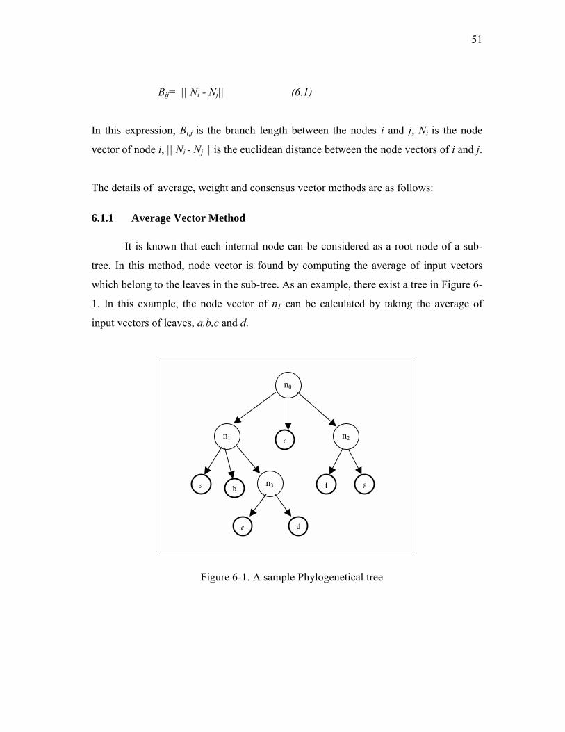
51

Bij= || Ni - Nj|| (6.1)

In this expression, Bi,j is the branch length between the nodes i and j, Ni is the node

vector of node i, || Ni - Nj || is the euclidean distance between the node vectors of i and j.

The details of average, weight and consensus vector methods are as follows:

6.1.1 Average Vector Method It is known that each internal node can be considered as a root node of a sub-

tree. In this method, node vector is found by computing the average of input vectors

which belong to the leaves in the sub-tree. As an example, there exist a tree in Figure 6-

1. In this example, the node vector of n1 can be calculated by taking the average of

input vectors of leaves, a,b,c and d.

Figure 6-1. A sample Phylogenetical tree

n0

n1 e n2

f ga n3b

c d

52

6.1.2 Weight Vector Method

It is pointed out that during the tree inference process each node corresponds to

a cell in Hierarchical SOM. Weight vectors of cells can be very good alternative for

node vectors because they are obtained by a training process and they can reflect the

characteristic properties of their leaves in their sub-trees.

6.1.3 Consensus Vector Method This method is similar to average vector but it does not use classic average

function. For each nucleotide position of the related sequences, (leaves of the sub-tree

that is originated from the node) the mostly found character state is given to the

corresponding position of the node vector. Suppose that sub-tree of a node has the

following leaves:

ATGC, AGGC, TTCA, ATAC

The number of nucleotide 'A' in the first position is three. So it is the mostly found

nucleotide in this position. Then first position of node vector will be 'A'. After the

evaluation of all positions, the node vector is found as 'ATGC'. As expected, actual

node vector is the numerical equivalent of this sequence.

6.2 Test method for Branch Length Estimation Quality

Justification of branch length estimation quality can be done by branch error

estimation method [2]. This method basically compares all pair wise distances of the

input data with the inferred distances in phylogenetical tree. Method is shortly

described below.

Suppose that a phylogenetical tree T is inferred from the given distance data

matrix which includes pair wise distances of n sequences. Error of tree E(T) can be

found by the following expression:

53

n n α E(T) ≡ ∑ ∑ wij |Dij – dij | (6.1) i=1 j≠i

dij : Distance value between sequences i and j in distance data matrix.

Dij: Distance value between sequences i and j in the inferred tree.

2

wij: Weight factors ( wij = 1/ dij )

α: Power value of absolute difference (α=2)

This expression takes the sum of all absolute differences between tree distances and

actual distances in input data. If inferred tree has good topology and estimations of

branch lengths are done well, value of E(T) will be minimized. In other words less

value means higher quality. In general, this function is not only used for finding the

errors of branch length estimation, it is used as an overall objective function by

distance-based methods.

6.3 Comparison of Branch Calculation Methods

In this topic, branch length estimation methods are compared by branch error

estimation method with all data sets. In Table 6-1, test results are given. Figure 6-2

includes the charts of table for better understanding.

Table 6-1. Test results of all data sets with different

edge length calculation methods

Data Sets

Sequence Number

Average Vector

Weight Vector

Consensus Vector

Tp53 10 6.56 6.86 39.42 Actin 14 10.78 4.09 33.09

Globin 20 31.56 17.06 111.17

Hemoglobin 34 115.81 76.28 558.92

Keratin 59 762.46 413.59 4009.53

HBV 100 2676.31 1713.24 24241.90

Myosin 200 11471.52 9905.56 128315.11

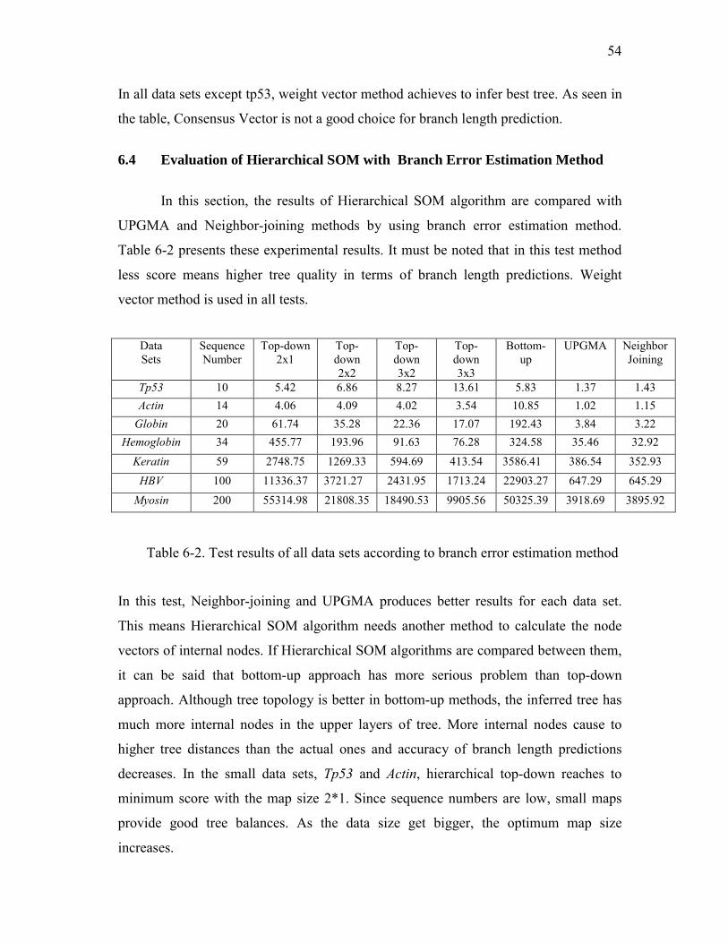
54

In all data sets except tp53, weight vector method achieves to infer best tree. As seen in

the table, Consensus Vector is not a good choice for branch length prediction.

6.4 Evaluation of Hierarchical SOM with Branch Error Estimation Method

In this section, the results of Hierarchical SOM algorithm are compared with

UPGMA and Neighbor-joining methods by using branch error estimation method.

Table 6-2 presents these experimental results. It must be noted that in this test method

less score means higher tree quality in terms of branch length predictions. Weight

vector method is used in all tests.

Table 6-2. Test results of all data sets according to branch error estimation method

In this test, Neighbor-joining and UPGMA produces better results for each data set.

This means Hierarchical SOM algorithm needs another method to calculate the node

vectors of internal nodes. If Hierarchical SOM algorithms are compared between them,

it can be said that bottom-up approach has more serious problem than top-down

approach. Although tree topology is better in bottom-up methods, the inferred tree has

much more internal nodes in the upper layers of tree. More internal nodes cause to

higher tree distances than the actual ones and accuracy of branch length predictions

decreases. In the small data sets, Tp53 and Actin, hierarchical top-down reaches to

minimum score with the map size 2*1. Since sequence numbers are low, small maps

provide good tree balances. As the data size get bigger, the optimum map size

increases.

Data Sets

Sequence Number

Top-down 2x1

Top-down 2x2

Top-down 3x2

Top-down 3x3

Bottom-up

UPGMA Neighbor Joining

Tp53 10 5.42 6.86 8.27 13.61 5.83 1.37 1.43 Actin 14 4.06 4.09 4.02 3.54 10.85 1.02 1.15

Globin 20 61.74 35.28 22.36 17.07 192.43 3.84 3.22 Hemoglobin 34 455.77 193.96 91.63 76.28 324.58 35.46 32.92

Keratin 59 2748.75 1269.33 594.69 413.54 3586.41 386.54 352.93 HBV 100 11336.37 3721.27 2431.95 1713.24 22903.27 647.29 645.29

Myosin 200 55314.98 21808.35 18490.53 9905.56 50325.39 3918.69 3895.92

55

Chapter 7

7. Conclusion and Future Work

In this study, firstly detailed information about phylogeny problem and self

organizing maps (SOM) are given. Secondly, Hierarchical SOM is proposed for

inferring phylogenetical tree problem. Two different types of Hierarchical SOM

algorithms are developed. One of them is top-down approach that constructs the tree

from the root to the terminal nodes. The other one, bottom-up approach, infers the tree

in the opposite direction, from the terminal nodes to the root. These algorithms

construct the tree topology, but estimation of branch lengths remain unsolved. Three

distinct methods are presented for this purpose, average, weight and consensus vector

methods.

In order to prove the efficiency of our methods, we used two testing methods.

First one is called topology testing method which evaluates the quality of tree topology.

The second one is branch error estimation method which is commonly used for quality

of branch length estimation. Hierarchical SOM algorithms are tested with seven

different data sets and the results of tests are compared with the results of Neighbor-

56

joining and UPGMA methods. It is proven that in terms of topology quality,

hierarchical SOM algorithms give better results than other methods in all data sets.

Hierarchical bottom-up SOM yields better results for large data sets according to the

topology test. The test efforts continued with fining tuning of SOM function

parameters. Different initial learning rates and neighborhood widths are tested for each

data set. The optimum parameter values are determined.

The study concludes with proposing some solutions for branch length prediction

problem. Three different solutions, average, weight and consensus vector methods are

presented and they are compared with each other by branch error estimation method.

Test results show that for the most of data sets weight vector method gives better

results.

Branch length prediction capability of Hierarchical SOM algorithms are

compared with UPGMA and Neighbor-joining by using branch error estimation

method. According to test results, Neighbor-joining and UPGMA methods are better

than Hierarchical SOM. This means much more effort is needed for branch length

prediction part of Hierarchical SOM.

Further improvements can be done for Hierarchical SOM algorithms. As stated

before, top-down approach uses fix map size at each iteration. This can bring some

restrictions to the topology. Hierarchical top-down SOM can decide different map sizes

for each iteration according to the number of inputs.

Branch length prediction problem must be studied much deeper. The prediction

methods presented in this study don’t give high quality trees in terms of branch lengths.

Especially node vectors of internal nodes can be chosen more accurately.

Neighbor-joining creates the tree in bottom-up manner and achieves better tree branch

predictions. So branch length estimation idea of Neighbor-joining can be adapted to

bottom-up hierarchical SOM.

8. Bibliography

[1] Hari Tammana, Phylogenetical Analysis, Lecture Notes,

http://www.msci.memphis.edu/~giri/compbio/f99/hari/hari.htm

[2] Swofford and Olsen, Phylogeny Reconstruction, Molecular Systematics

Phylogenetical Trees, Molecular Biology Chapter 6

[3] Reinhard Diestel, Graph Theory, Chapter 1, 1997, pp 12

[4] David L. Swofford PAUP(software package for inference of evolutionary

trees) package version 4.0, http://paup.csit.fsu.edu/index.html

[5] Joe Felsenstein, PHYLIP (Phylogeny Inference Package) version 3.5

Department of Genetics, University of Washington

http://www.cmbi.kun.nl/bioinf/PHYLIP

[6] Kohonen T. The Self-Organizing Map Proceedings of the IEEE vol. 78 no. 9,

pp 1464-1480, September 1990

[7] Martin Beveridge, Lecture Notes, Computer Studies Dept. Napier University

http://www.dcs.napier.ac.uk/hci/martin/msc/node18.html

[8] Jens Hanke and Jens G.Reich , CABIOS, Kohonen map as a visualization tool

for the analysis of protein sequences, Bioinformatics Vol.12 no.6 pp 447-454

1996

58

[9] Joaquin Dopazo, Jose Maria Carazo, Phylogenetic reconstruction using an

unsupervised growing neural network that adopts the topology of a

phylogenetic tree, Journal of Molecular Evolution, 1997.

[10] Fritzke B, Growing cell structures –a self organizing network for

unsupervised and supervised learning, Neural Networks 7: pp:1141-1160,1994

[11] National Center for Biotechnology Information http://www.ncbi.nlm.nih.gov/

[12] Saitou N, Nei M, The neighbor-joining method :a new method for

reconstructing phylogenetic trees. Mol.Biol Evol 4:pp:406-425

[13] Edgardo A. Ferran, Pascual Ferrara Unsupervised Clustering of Proteins,

Artificial Neural Networks 1991, pp:1341-1345

[14] M.D.Hendy and D.Penny, Branch and bound algorithms to determine minimal

evolutionary trees, Mathematical Biosciences, 60:133-142,1982

[15] Ferran EA, Pflugfelder B, A hybrid method to cluster protein sequences based

on statistic and artificial neural networks, Comput. Appl. Biosci 9:671-

680,1993

[16] W. H. E. Day, Computational complexity of inferring phylogenies from

dissimilarity matrices.Bull. Math. Biol. 49(4):461-467, 1987.

[17] Henikoff, S. & Henikoff, J. G,Amino acid substitution matrices from protein

blocks. Proc. Natl. Acad. Sci. USA, 89, 10915-10919,1992

[18] J.Lampinen and E.Oja, Clustering Properties of Hierarchical Self Organizing

Maps, Journal of Mathematical Imaging and Vision, Vol.2, pp.261-272, 1992.

APPENDIX

9. Some Data Sets and Sample Inferred Trees In this section, contents of data sets Tp53, Actin, and Globin are given. For each set, inferred trees by Hierarchic SOM and Neighbor-joining methods are also shown. 9.1 Tp53 >Homo sapiensClone MGC:3578-1 ATGATGCTGGGGAGCTTGGCGCCTGACCCAGGATCTAGAAGGCACTCTGGGCAGGCCGCGCTCCGCCCAC >OryziasLatipesTumorSuppressor ATGGATCCTGTACCCGACCTGCCCGAGAGCCAAGGTTCTTTTCAAGAACTCTGGGAGACTGTTTATCCTC >XiphophorusMaculatusStrainRioJamapa ATGGAGGAGGCGGATCTCACACTGCCTTTGAGTCAGGACACCTTCCATGACTTATGGAACAATGTGTTTT >XiphophorusHelleriStrainRioSarabia ATGGAGGAGGCGGACCTCACCCTGCCTTTGAGTCAGGACACCTTCCATGACTTATGGAACAATGTTTTTT >XiphophorusMaculatusSuppressorOrtholog GATCCGAGATGACCACAATCCTTCTGAGCTTTATGTGCAACAGCTCCTGCATGGGAGGCATGAACCGGAG >Human p53-1 ATGGAGCAGCCGCAGTCAGATCCTAGCGTCGAGCCCCCTCTGAGTCAGGAAACATTTTCAGACCTATGGA >Human p53-2 ATGGAGGAGCCGCAGTCAGATCCTAGCGTCGAGCCCCCTCTGAGTCAGGAAACATTTTCAGACCTATGGA

60

>Human p53CellularTumorAntigen ATGGAGGATCCGCAGTTAGGTCCTAGCGTCGAGCCCCCTTTGAGTCAGGAAACATTTTCAGACCTATGGA >Human p53CellularTumorAntigenmRNA ATGGAGGAGCCGCAGTCAGATCCTAGCGTCGAGCCCCCTTTGAGTCAGGAAACATTTTCAGACCTATGGA >Homo sapiensClone MGC:3578 ATGATGGTGGGGAGCTTGGCGCCTGACCCAGGATCTAGAAGGCACTCTGGGCAGGCCGCGCTCCGCCCAC-2 Tree by Top-down 2*2 Hierarchical SOM Tree by Bottom-up Hierarchical SOM

Xiphphorus MaculatusStrain Rio Jamapa

Xiphphorus Helleris Strain Rio Sarapa

Orzyias Latipes Tumor

Homo Sapiems Clone MGC 3578-1

Homo Sapiems Clone MGC 3578-2

Xiphphorus MaculatusSuppressor Ortholog

Human-p53-1

Human-p53-2

Human p53 Cellular Tumor Antigen

Human p53 Cellular Tumor Antigen mRNA

Xiphphorus MaculatusStrain Rio Jamapa

Xiphphorus Helleris Strain Rio Sarapa

Orzyias Latipes Tumor

Homo Sapiems Clone MGC 3578-1

Homo Sapiems Clone MGC 3578-2

Xiphphorus Maculatus Suppressor Ortholog

Human-p53-1

Human-p53-2

Human p53 Cellular Tumor Antigen

Human p53 Cellular Tumor Antigen mRNA

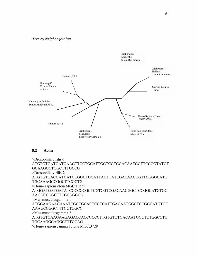
61

Tree by Neigbor-joining 9.2 Actin >Drosophila virilis-1 ATGTGTGATGATGAAGTTGCTGCATTGGTCGTGGACAATGGTTCCGGTATGTGCAAGGCTGGCTTTGCCG >Drosophila virilis-2 ATGTGTGACGATGATGCGGGTGCATTAGTTATCGACAACGGTTCGGGCATGTGCAAAGCCGGCTTCGCTG >Homo sapiens cloneMGC:10559 ATGGATGATGATATCGCCGCGCTCGTCGTCGACAACGGCTCCGGCATGTGCAAGGCCGGCTTCGCGGGCG >Mus musculusgamma 1 ATGGAAGAAGAAATCGCCGCACTCGTCATTGACAATGGCTCCGGCATGTGCAAAGCCGGCTTTGCTGGCG >Mus musculusgamma 2 ATGTGTGAAGAAGAGACCACCGCCCTTGTGTGTGACAATGGCTCTGGCCTGTGCAAGGCAGGCTTTGCAG >Homo sapiensgamma 1clone MGC:3728

Xiphphorus Maculatus Strain Rio Jamapa

Xiphphorus Helleris Strain Rio Sarapa

Orzyias Latipes Tumor

Homo Sapiems Clone MGC 3578-1

Homo Sapiems Clone MGC 3578-2

Xiphphorus Maculatus Suppressor Ortholog

Human-p53-1

Human-p53-2

Human p53 Cellular Tumor Antigen

Human p53 Cellular Tumor Antigen mRNA

62

ATGGAAGAAGAGATCGCCGCGCTGGTCATTGACAATGGCTCCGGCATGTGCAAAGCTGGTTTTGCTGGGG >Oryzias latipes ATGGATGATGACATTGCCGCACTGGTTGTTGACAACGGATCTGGCATGTGCAAAGCTGGATTCGCTGGAG >Oxytricha fallax ATGTCAGACCAACAAACTTGCGTTATTGATAACGGTTCAGGAGTCGTCAAGGCTGGTTTCGCCGGTGAGG >Salmosalarfastmyotomalmuscle ATGTGTGACGACGACGAGACTACTGCTCTTGTGTGCGACAATGGCAGCGGCCTTGTGAAGGCTGGCTTCG >Salmotruttacardiacmuscle ATGTGTGACGACGACGAGACTACCGCCCTCGTGTGTGACAACGGCTCTGGCCTCGTCAAGGCTGGGTTCG >Ambystoma mexicanum cardia ATGTGCGACGATGAAGAGGTCACCGCCCTCGTGTGCGACAACGGCTCCGGCCTGGTGAAGGCTGGCTTCG >Rhodeus notatus ATGGATGATGAAATTGCCGCACTGGTTGTTGACAACGGATCCGGTATGTGCAAAGCCGGATTCGCTGGAG >Setaria italica ATGGCGGACGGTGAAGATATCCAGCCCCTTGTCTGCGACAATGGCACCGGCATGGTCAAGGCCGGTTTCG >Magnolia denudata ATGGCTGATGGTGAAGATATTCAACCCCTTGTCTGTGACAATGGAACTGGAATGGTGAAGGCTGGATTAG Tree by Top-down 2*2 Hierarchical SOM

Rhodeus notatus Salmasalar fast myotomalmuscle

Salmatruttacardiac muscle Ambystoma

mexicanum cardiac

Oxytricha fallax Mus muscullus gamma2

Drosophila virilis1

Drosophila virilis2

Setaria Italica

Magnolia denudata

Homo sapiens MGC10559

Homo sapiens gammaclone

Mus musculus gamma1

Oryzias latipes

63

Tree by Bottom-up Hierarchical SOM Tree by Neigbor-joining

Oxytricha fallax Mus muscullus gamma2

Drosophila virilis1

Drosophila virilis2

Setaria Italica

Magnolia denudata

Salmasalar fast myotomal muscle

Salmatrutta cardiac muscle

Ambystoma mexicanum cardiac Rhodeus notatus

Homo sapiens MGC10559

Homo sapiens gammaclone

Mus musculus gamma1

Oryzias latipes

Oxytricha fallax

Mus muscullus gamma2

Drosophila virilis1

Drosophila virilis2

Setaria Italica

Magnolia denudata

Salmasalar fast myotomal muscle

Salmatrutta cardiac muscle

Ambystoma mexicanum cardiac

Rhodeus notatus

Homo sapiens MGC10559

Homo sapiens gammaclone

Mus musculus gamma1

Oryzias latipes

64

9.3 Globin >SminthopsisCrassicaudataOmega ATGGTGAACTGGACAGCAGAAGAGAAACAGGCCATTTCAACCATCTGGGCCAAAATTGACATCGAGGAAG >MacropusEugeniiOmega ATGGTGCACTGGACAGCAGAAGAGAAACAGATCATTTTAGCCATCTGGGCCAAGATTGACATCGAGGAAG >CallithrixJacchusGamma1 ATGAGTAATTTCACAGCTGAGGACAAGGCTGCTATCACTAGCCTGTGGGCCAAGGTGAATGTGGAAGATG >CallithrixJacchusGamma3 ATGAGTAATTTCACAGCTGAGTACAAGGCTGCTATCACTAGCCTGTGGGCCAAGGTGAATGTGGAAGATG >CallicebusMolochGamma2 ATGAGTAATTTCACAGCTGAGGACAAGGCTGCCATCACGAGCCTGTGGGGCAAGGTGAATGTGGAAGATG >ChiropotesSatanasGamma1 ATGGGAAATTTCACAGCTGAGGACAAGGCTGCTATCACTAATCTGTGGGGCAAGGTGAACGTGGAAGATG >AotusNancymaaeHybridGamma1/gamma2 ATGAGTAATTTCACAGCTGAGGACAAGGCTGCTATCACTGGCCTGTGGGCCAAGGTGAATGTGGAAGATG >SaimiriUstusHybridGamma1/gamma2 ATGAGTAATGTCACAGCTGAGGACAAGGCTGCTATCACTAGCCTGTGGGCCAAGGTGAATGTGGAAGATG >CaenorhabditisElegans ATGTCGATGAACCGTCAAGAAATTAGTGATCTCTGTGTGAAGTCCCTTGAAGGACGAATGGTTGGAACTG >NototheniaCoriicepsAlpha ATGAGTCTCTCCGACAAAGACAAGGCAGCAGTCAAGGCTCTGTGGAGCAAGATCGGCAAGTCAGCTGATG >NototheniaAngustataBeta ATGAGTCTCTCCGACAAAGACAAGGCAGCAGTCAGGGCTCTGTGGAGCAAGATCGGCAAGTCAGCTGATG >HomoSapiensMutant ATGGTGCACCTGACTCCTGAGGAGAAGTCTGCCGTTACTGCCCTGTGGGGCAAGGTGAACGTGGATGAAG >CaenorhabditisElegans ATGTCGATTAACCGTCAAGAAATTAGTGATCTCTGTGTGAAGTCCCTTGAAGGACGAATGGTTGGAACTG >MermisNigrescensEye ATGGTAGTAAATTTGGACATTCTTCGGGCGCAATTGGCCAAATTGCCCATCAACGAGTTCAACGGCCCTA >EquusZebraAlpha 1

65

ATGGTGCTGTCTGCCGCCGACAAGACCAACGTCAAGGCCGCCTGGAGTAAGGTTGGCGGCAACGCTGGCG >DanioRerioEmbryonic1 beta ATGGTTGTGTGGACAGACTTCGAGAAGGCCACCATTCAAGATATCTTCGCCAAGGCTGACTACGACGTCA >HorseBIalpha-1 ATGGTGCTGTCTGCCGCCGACAAGACCAACGTCAAGGCCGCCTGGAGTAAGGTTGGCGGCCACGCTGGCG >CebusApella ATGAGTAATTTCATAGCTGAGGACAAGGCTGCTATCACTAGCCTGTGGGCCAAGGTGAATGTGGAAGATG >AotusAzaraiHybrid(gamma1/gamma2) ATGAGTAAGTTCACAGCTGAGGACAAGGCTGCTATCACTAGCCTGTGGGCCAAGGTGAATGTGGAAGATG >CerebratulusLacteusNeural ATGGTTAACTGGGCTGCCGTCGTTGATGACTTTTACCAAGAGCTTTTCAAGGCCCACCCTGAGTACCAAA Tree by Top-down 2*2 Hierarchical SOM

Caenor Habditis Elegans-1

Caenor Habditis Elegans-2

Notothenia Coriiceps Alpha

Notohenia Angustata beta

Equus Zebra Alpha1

Horse Bialpha-1

Mermis Nigres cens Eye

Danio Rerio Embryonic beta

Cerevratulus Lacteus Neural

Chiropotes Satanas Gamma1 Callicebus

Moloch Gamma2

Aotus Azarai Hybrid

Callithrix Jacchus Gamma3

Saimiri Ustus Hybrid

Cebus Apella

Aotus Nancymae Hybrid

Callithrix Jacchus Gamma1

Notothenia Angustata Beta

Sminthopsis Crassic Audata Omega

Macropus Eugenii Omega

66

Tree by Bottom-up Hierarchical SOM

Aotus Azarai Hybrid

Callithrix Jacchus Gamma3

Saimiri Ustus Hybrid

Cebus Apella

Aotus Nancymae Hybrid

Callithrix Jacchus Gamma1

Caenor Habditis Elegans-1

Caenor Habditis Elegans-2

Notothenia Coriiceps Alpha

Notohenia Angustata beta

Equus Zebra Alpha1

Horse Bialpha-1

Mermis Nigres cens Eye

Danio Rerio Embryonic beta

Cerevratulus Lacteus Neural

Callicebus Moloch Gamma2

Notothenia Angustata Beta

Sminthopsis Crassic Audata Omega

Macropus Eugenii Omega

Chiropotes Satanas Gamma1

67

Tree by Neigbor-joining

Cebus Apella

Aotus Nancymae Hybrid

Callithrix Jacchus Gamma1

Saimiri Ustus Hybrid

Aotus Azarai Hybrid

Callicebus Moloch Gamma2

Chiropotes Satanas Gamma1

Macropus Eugenii Omega

Sminthopsis Crassic Audata Omega

Danio Rerio Embryonic beta

Notothenia Coriiceps Alpha

Notohenia Angustata beta

Equus Zebra Alpha1

Horse Bialpha-1

Mermis Nigres cens Eye

Cerevratulus Lacteus Neural

Caenor Habditis Elegans-1

Caenor Habditis Elegans-2