INFERRING MECHANISM-BASED GENE REGULATORY NETWORK MODELS

FROM EXPRESSION AND SEQUENCE DATA

by

Yue Pan

A dissertation submitted in partial fulfillment of

the requirements for the degree of

Doctor of Philosophy

(Computer Sciences)

at the

UNIVERSITY OF WISCONSIN–MADISON

2009

c© Copyright by Yue Pan 2009

All Rights Reserved

i

To Mom, Dad, and Ru for unconditional love and support.

&

To statistician George Box for his saying “all models are wrong, but some are useful”.

ii

ABSTRACT

Gene regulatory networks (GRNs) function as the master plan for controlling the expression

of genes in living cells. Understanding the interactions between regulatory factors and their target

genes in such regulatory networks is a fundamental and challenging problem for experimental and

computational biologists. The main goal of this dissertation is to develop novel statistical models

and computational algorithms to better understand which regulators control which genes and how,

by analyzing gene expression and genomic sequence data.

In contrast to most previous methods for inferring GRN models from high-throughput data

sources, the approach of this dissertation improves the state of the art by inferring models that

directly address the underlying mechanism of regulator-gene interactions.

My approach involves representing and learning the key kinetic parameters in regulation func-

tions that govern transcription rates as functions of features in the genomic sequence. Thus, this

approach provides a more mechanistic representation of regulator-gene relationships and offers

better predictive accuracy and explanatory power than alternative models.

My approach also involves refining the structure of prior network models by discovering hid-

den regulators in gene regulatory networks, based on both expression and sequence data. This

new framework provides a tool for biologists to discover new regulatory relationships with high

precision.

iii

ACKNOWLEDGMENTS

I am indebted to my advisor, Professor Mark Craven, for his guidance and support over thelast five years. Mark taught me a wide variety of research skills: Identifying important topics,crafting novel ideas, developing rigorous algorithms, crisply analyzing and understanding results,pushing through or getting out of dead ends, being critical and skeptical of existing methods butin a constructive way, writing high-standard scientific documents, and so on. Mark also showedme, as my class teacher and presentation critic, efficient ways to convey scientific thoughts: Beingconcise and precise, standing in the shoes of the audience, illustrating complicated procedures withstraightforward figures, and so forth. I truly feel that I have learned a lot from a brilliant researcherand teacher. Outside science, I also observed Mark interact with his colleagues and students with asense of humor to maintain a friendly working environment. All of the above have influenced mygraduate study and will help me throughout my future career.

I would like to thank Professors Jude Shavlik and David Page for not only serving on my prelimand thesis committees, but also, as my class teachers, for introducing me to the worlds of artificialintelligence, machine learning and bioinformatics. Jude also offered valuable comments on mytalks and writings, ranging from fundamental algorithmic ideas to axes on figures and hyphens inthe bibliography. David always had his office door open so I could pop in for AI questions.

I also want to acknowledge Professors Colin Dewey and Gheorghe Craciun for serving on mythesis committee and offering insightful feedback. The same gratitude goes to my other prelimcommittee members: Professors Tim Donohue and Michael Ferris.

I thank Mark, Jude, David, Professors Michael Coen and Jerry Zhu for their frank advice as Iplan my career.

I was very happy to work as a Research Intern in the Machine Learning and Applied StatisticsGroup at Microsoft Research in Seattle in 2007. I thank my mentors, Dr. Bo Thiesson and Dr.Alex Bocharov, for giving me the freedom to choose a cutting-edge machine learning researchproject. Bo taught me state-of-the-art Bayesian statistics, while Alex educated me on advancedC++ coding skills. Their trust in me, efficient communication with me, the independence I had,and the excellent working environment made my internship the most scientifically fruitful periodof the last several years. In the meantime, I appreciate Microsoft Research for allowing me to tourthe gorgeous mountains, lakes, and national parks around the Seattle area—those sight-seeing tripsreally leave wonderful and long-lasting memories.

At the early stage of my graduate study, I worked with Professor Beth Burnside on improvingan expert system for breast cancer prediction. I thank her for offering the opportunity to apply mydata mining skills to an important real-world problem in medical informatics. She helped me to

iv

publish my first scientific paper and to present my research work in front of a large audience at aconference for the first time.

During my graduate study, various students, post-docs, and visitors in the Craven lab, theUW machine learning group and the BACTER Institute have made valuable contributions to mypersonal and professional life. I am grateful to my collaborators Tim Durfee and Joe Bockhorst,who assisted me in the work described in Chapter 4. Keith Noto was very generous to share datasets, a prelim document template, and computer scripts with me. Keith also reviewed one draft ofmy ISMB paper and offered helpful comments.

Dave Andrzejewski, Joe Bockhorst, Debbie Chasman, Deborah Muganda, Keith Noto, SoumyaRay, Burr Settles, and Adam Smith listened to my talks at our lab meetings and gave me valuablesuggestions. Hidayath Ansari, Bess Berg, Sean McIlwain, and Adam Smith have been great officemates along my PhD journey; they never felt bothered whether I interrupted their work for seri-ous help or trivial chatting. David Baumler, Vitor Santos Costa, Jesse Davis, Omar Demerdash,Frank DiMaio, Yann Dufour, Ines Dutra, Mike Gilson, Mark Goadrich, Larry Hendrix, Eric Lantz,Jie Liu, Xiao-Yu Liu, Richard Maclin, Sean McIlwain, Michael Molla, Houssam Nassif, LouisOliphant, Irene Ong, Beverly Seavey, Julie Simons, Ameet Soni, Jan Struyf, Vanitha Suresh, LisaTorrey, Michael Waddell, Trevor Walker, and others helped me in my graduate study or suggestedtips on Madison’s daily life, in various ways.

I thank the following people for assisting me in writing this dissertation. Dr. Madeline Fisherfrom the BACTER Institute offered comments on the structure and flow of the first chapter I wrote(Chapter 3), which subsequently influenced my writing style for the rest of the chapters (e.g.,always keeping in mind both logical structure and sentence linkage). She also read most of myother chapters and is very keen to spot both semantic and syntactic errors—I could not ask fora better “outside” reviewer. Hidayath was very kind to allow me to use some software on hisworkstation, which made the otherwise tedious LATEX editing a “WYSIWYG”, breezy experience.Burr supplied me a thesis template without charging me a penny; he and Adam also told me tricksto making high-quality vector figures for publication.

I also want to acknowledge my friends in Madison for the fun they brought to me, the trips weshared, the movies we watched, etc. In particular, I thank my fellow badminton club friends for themany exhausting but exciting games we played; I also thank badminton coach Ronnie Carda forteaching me club-level skills.

Special acknowledgment goes to Professor Julie Mitchell and the BACTER Institute. Fundingfrom the DOE GTL Program and the UW BACTER Institute supported my thesis research andvarious conference travels.

Finally, I am deeply grateful to my family from the bottom of my heart. My parents alwaysunderstand, encourage and support me, and are ready to do whatever they can to help me eventhough they are far away in China. My younger brother always believes in my ability to climbmountains in the real-world and in science, and cares a whole lot about my studies and career. Iam at a loss for words on how to thank my wife and best friend, Xiao Ru. Ru has been supportiveon every aspect and moment of this journey while conducting her doctoral research at the sametime. For everything that was and will be, thank you! Now that we are both armed with PhDs, Iam ready to give her more support in the new era of our lives...

DISCARD THIS PAGE

v

TABLE OF CONTENTS

Page

ABSTRACT . . . . . . . . . . . . . . . . . . . . . . . . . . . . . . . . . . . . . . . . . . ii

LIST OF TABLES . . . . . . . . . . . . . . . . . . . . . . . . . . . . . . . . . . . . . . . viii

LIST OF FIGURES . . . . . . . . . . . . . . . . . . . . . . . . . . . . . . . . . . . . . . ix

1 Introduction . . . . . . . . . . . . . . . . . . . . . . . . . . . . . . . . . . . . . . . . 1

1.1 Issues in Gene Regulatory Network Reconstruction . . . . . . . . . . . . . . . . . 21.2 Extending the State of the Art . . . . . . . . . . . . . . . . . . . . . . . . . . . . 6

1.2.1 Connecting Regulation Functions to the Genome . . . . . . . . . . . . . . 61.2.2 Discovering Regulators . . . . . . . . . . . . . . . . . . . . . . . . . . . . 71.2.3 Handling Unmeasured Events . . . . . . . . . . . . . . . . . . . . . . . . 8

1.3 Dissertation Motivation . . . . . . . . . . . . . . . . . . . . . . . . . . . . . . . . 91.4 Dissertation Statement . . . . . . . . . . . . . . . . . . . . . . . . . . . . . . . . 101.5 Dissertation Outline . . . . . . . . . . . . . . . . . . . . . . . . . . . . . . . . . . 11

2 Background . . . . . . . . . . . . . . . . . . . . . . . . . . . . . . . . . . . . . . . . 12

2.1 Biological Concepts and Techniques . . . . . . . . . . . . . . . . . . . . . . . . . 122.1.1 Gene Regulation . . . . . . . . . . . . . . . . . . . . . . . . . . . . . . . 122.1.2 Experimental Techniques . . . . . . . . . . . . . . . . . . . . . . . . . . . 18

2.2 Computational Models and Methods . . . . . . . . . . . . . . . . . . . . . . . . . 202.2.1 Bayesian Networks . . . . . . . . . . . . . . . . . . . . . . . . . . . . . . 202.2.2 Gene Expression Clustering . . . . . . . . . . . . . . . . . . . . . . . . . 242.2.3 Motif Discovery . . . . . . . . . . . . . . . . . . . . . . . . . . . . . . . 29

2.3 Summary . . . . . . . . . . . . . . . . . . . . . . . . . . . . . . . . . . . . . . . 31

3 Related Work . . . . . . . . . . . . . . . . . . . . . . . . . . . . . . . . . . . . . . . 34

3.1 Regulatory Network Modeling Methods . . . . . . . . . . . . . . . . . . . . . . . 353.1.1 Model Representation . . . . . . . . . . . . . . . . . . . . . . . . . . . . 353.1.2 Qualitative vs. Quantitative . . . . . . . . . . . . . . . . . . . . . . . . . 37

vi

Page

3.1.3 Static vs. Dynamic . . . . . . . . . . . . . . . . . . . . . . . . . . . . . . 383.1.4 Expression vs. Activity . . . . . . . . . . . . . . . . . . . . . . . . . . . . 393.1.5 Regulator Mapping vs. Regulator Discovery . . . . . . . . . . . . . . . . . 393.1.6 My Approach vs. Previous Approaches . . . . . . . . . . . . . . . . . . . 40

3.2 Gene Expression Clustering Methods . . . . . . . . . . . . . . . . . . . . . . . . 413.2.1 Representative Clustering Methods . . . . . . . . . . . . . . . . . . . . . 413.2.2 The Adapted Clustering Method in My Approach . . . . . . . . . . . . . . 44

3.3 Motif Discovery Methods . . . . . . . . . . . . . . . . . . . . . . . . . . . . . . . 453.3.1 Methods for One Species Multiple Genes Scenario . . . . . . . . . . . 453.3.2 Methods for Multiple Species One Gene Scenario . . . . . . . . . . . . 483.3.3 Methods for Multiple Species Multiple Genes Scenario . . . . . . . . . 493.3.4 Methods Employed in My Approach . . . . . . . . . . . . . . . . . . . . . 50

3.4 Motif Filtering and Ranking Methods . . . . . . . . . . . . . . . . . . . . . . . . 513.5 Summary . . . . . . . . . . . . . . . . . . . . . . . . . . . . . . . . . . . . . . . 54

4 Connecting Quantitative Regulatory Network Models to the Genome . . . . . . . . 55

4.1 Introduction and Motivation . . . . . . . . . . . . . . . . . . . . . . . . . . . . . 554.2 Approach . . . . . . . . . . . . . . . . . . . . . . . . . . . . . . . . . . . . . . . 57

4.2.1 A Kinematic Model of Transcriptional Regulation . . . . . . . . . . . . . 574.2.2 Considering RNAP as Regulator . . . . . . . . . . . . . . . . . . . . . . 604.2.3 Modeling Regulator Binding-Strength and Productivity

using Genomic-Sequence Features . . . . . . . . . . . . . . . . . . . . . 614.2.4 Accounting for Sequence Uncertainty . . . . . . . . . . . . . . . . . . . . 654.2.5 Network Architecture . . . . . . . . . . . . . . . . . . . . . . . . . . . . . 674.2.6 Parameter Learning . . . . . . . . . . . . . . . . . . . . . . . . . . . . . 68

4.3 Empirical Evaluation . . . . . . . . . . . . . . . . . . . . . . . . . . . . . . . . . 694.3.1 Data Sets . . . . . . . . . . . . . . . . . . . . . . . . . . . . . . . . . . . 694.3.2 Evaluating Model Accuracy . . . . . . . . . . . . . . . . . . . . . . . . . 714.3.3 Evaluating Model Explanatory Power . . . . . . . . . . . . . . . . . . . . 74

4.4 Summary . . . . . . . . . . . . . . . . . . . . . . . . . . . . . . . . . . . . . . . 78

5 Discovering Hidden Regulators of Gene Regulatory Networks . . . . . . . . . . . . 79

5.1 Introduction . . . . . . . . . . . . . . . . . . . . . . . . . . . . . . . . . . . . . . 795.2 Motivation . . . . . . . . . . . . . . . . . . . . . . . . . . . . . . . . . . . . . . . 815.3 Previous Methods vs. My Method . . . . . . . . . . . . . . . . . . . . . . . . . . 825.4 Approach . . . . . . . . . . . . . . . . . . . . . . . . . . . . . . . . . . . . . . . 85

5.4.1 Initializing the Network Structure . . . . . . . . . . . . . . . . . . . . . . 865.4.2 Identifying Weakly Explained Genes . . . . . . . . . . . . . . . . . . . . 89

vii

Page

5.4.3 Clustering Genes Based on Error Profiles . . . . . . . . . . . . . . . . . . 905.4.4 Motif Finding for Clustered Genes . . . . . . . . . . . . . . . . . . . . . . 925.4.5 Filtering and Ranking Candidate Motifs . . . . . . . . . . . . . . . . . . . 935.4.6 Proposing Hidden Regulators . . . . . . . . . . . . . . . . . . . . . . . . 99

5.5 Empirical Evaluation . . . . . . . . . . . . . . . . . . . . . . . . . . . . . . . . . 1005.5.1 Experimental Data . . . . . . . . . . . . . . . . . . . . . . . . . . . . . . 1005.5.2 Evaluation Methodology . . . . . . . . . . . . . . . . . . . . . . . . . . . 1035.5.3 The Value of Filtering Methods . . . . . . . . . . . . . . . . . . . . . . . 1045.5.4 The Value of Ranking Methods . . . . . . . . . . . . . . . . . . . . . . . 1075.5.5 The Effect of Motif Finders . . . . . . . . . . . . . . . . . . . . . . . . . 111

5.6 A Case Study of Hidden Regulator Discovery . . . . . . . . . . . . . . . . . . . . 1195.7 Summary . . . . . . . . . . . . . . . . . . . . . . . . . . . . . . . . . . . . . . . 121

6 Additional Work in Learning Bayesian Network Modelsfor Breast Cancer Prediction . . . . . . . . . . . . . . . . . . . . . . . . . . . . . . . 123

6.1 Introduction . . . . . . . . . . . . . . . . . . . . . . . . . . . . . . . . . . . . . . 1236.2 Materials and Methods . . . . . . . . . . . . . . . . . . . . . . . . . . . . . . . . 124

6.2.1 Model Structure . . . . . . . . . . . . . . . . . . . . . . . . . . . . . . . 1246.2.2 Software and Data . . . . . . . . . . . . . . . . . . . . . . . . . . . . . . 1266.2.3 Training and Evaluation . . . . . . . . . . . . . . . . . . . . . . . . . . . 127

6.3 Results . . . . . . . . . . . . . . . . . . . . . . . . . . . . . . . . . . . . . . . . . 1276.3.1 The Effect of the Tuning Set . . . . . . . . . . . . . . . . . . . . . . . . . 1276.3.2 The Effect of Missing Values . . . . . . . . . . . . . . . . . . . . . . . . . 1286.3.3 The Effect of the Training Set Size . . . . . . . . . . . . . . . . . . . . . . 128

6.4 Summary . . . . . . . . . . . . . . . . . . . . . . . . . . . . . . . . . . . . . . . 128

7 Conclusions . . . . . . . . . . . . . . . . . . . . . . . . . . . . . . . . . . . . . . . . 130

7.1 Summary of Contributions . . . . . . . . . . . . . . . . . . . . . . . . . . . . . . 1307.2 Future Directions . . . . . . . . . . . . . . . . . . . . . . . . . . . . . . . . . . . 1327.3 Final Remarks . . . . . . . . . . . . . . . . . . . . . . . . . . . . . . . . . . . . . 134

Bibliography . . . . . . . . . . . . . . . . . . . . . . . . . . . . . . . . . . . . . . . . . . 136

DISCARD THIS PAGE

viii

LIST OF TABLES

Table Page

2.1 Gene expression similarity and distance measures . . . . . . . . . . . . . . . . . . . . 26

4.1 Average relative error of various models on both data sets . . . . . . . . . . . . . . . 72

5.1 Accuracy (TP/FP) of four filters in seven lesion tests using the left-out TFs as refer-ence and PhyloCon as the motif finder . . . . . . . . . . . . . . . . . . . . . . . . . . 106

5.2 Accuracy (TP/FP) of four filters in seven lesion tests using known E. coli TFs asreference and PhyloCon as the motif finder . . . . . . . . . . . . . . . . . . . . . . . 106

5.3 Accuracy (TP/FP) of four filters in seven lesion tests using the left-out TFs as refer-ence and MEME as the motif finder . . . . . . . . . . . . . . . . . . . . . . . . . . . 118

5.4 Accuracy (TP/FP) of four filters in seven lesion tests using known E. coli TFs asreference and MEME as the motif finder . . . . . . . . . . . . . . . . . . . . . . . . . 118

6.1 Diagnosis of breast diseases represented in a Bayesian network model . . . . . . . . . 126

DISCARD THIS PAGE

ix

LIST OF FIGURES

Figure Page

1.1 Task of regulatory-network reconstruction . . . . . . . . . . . . . . . . . . . . . . . . 3

1.2 Illustration of a transcription factor binding to DNA . . . . . . . . . . . . . . . . . . 4

2.1 The central dogma of molecular biology . . . . . . . . . . . . . . . . . . . . . . . . . 13

2.2 A regulatory path between a transcription factor and a target gene . . . . . . . . . . . 16

2.3 Example gene regulatory networks . . . . . . . . . . . . . . . . . . . . . . . . . . . . 17

2.4 Example application of microarray technology . . . . . . . . . . . . . . . . . . . . . 19

2.5 Example conditional independence . . . . . . . . . . . . . . . . . . . . . . . . . . . 22

2.6 Example gene-expression clustering . . . . . . . . . . . . . . . . . . . . . . . . . . . 28

2.7 Example position specific probability matrix and sequence logo . . . . . . . . . . . . 30

2.8 How PhyloCon works . . . . . . . . . . . . . . . . . . . . . . . . . . . . . . . . . . 32

4.1 A kinematic model of transcription regulation by a single activator . . . . . . . . . . . 59

4.2 States and transitions for a two-regulator promoter . . . . . . . . . . . . . . . . . . . 60

4.3 Representing binding-strength parameters as a function of sequence features . . . . . 63

4.4 Representing a binding site when there is uncertainty about its position . . . . . . . . 66

4.5 Overlap in induced genes across carbon sources . . . . . . . . . . . . . . . . . . . . . 71

4.6 Cumulative error distributions of various models . . . . . . . . . . . . . . . . . . . . 73

4.7 Inferred available RNAP concentrations in carbon shift experiments . . . . . . . . . . 75

x

Figure Page

4.8 Agreement between predicted and measured expression values . . . . . . . . . . . . . 77

4.9 The most contributing bases of the -35 and -10 regions vs. consensus . . . . . . . . . 78

5.1 Illustration of the expression clustering-based approach to regulator discovery . . . . . 83

5.2 Flow of the hidden regulator discovery approach . . . . . . . . . . . . . . . . . . . . 87

5.3 Limitation of clustering gene expression profiles . . . . . . . . . . . . . . . . . . . . 91

5.4 A histogram illustrating the motif length distribution of known E. coli transcriptionfactors from RegulonDB . . . . . . . . . . . . . . . . . . . . . . . . . . . . . . . . . 94

5.5 Histograms illustrating the distributions of the fraction of information content of thefour nucleotides in known E. coli motifs from RegulonDB . . . . . . . . . . . . . . . 96

5.6 Known TF-gene relationships in oxygen-shift data set . . . . . . . . . . . . . . . . . 102

5.7 Precision-TP curves for the GlpR lesion test . . . . . . . . . . . . . . . . . . . . . . . 108

5.8 Precision-TP curves for the Fis lesion test . . . . . . . . . . . . . . . . . . . . . . . . 109

5.9 Precision-TP curves for the IHF lesion test . . . . . . . . . . . . . . . . . . . . . . . 110

5.10 Comparison of three ranking methods on unfiltered candidate motifs for the GlpRlesion test . . . . . . . . . . . . . . . . . . . . . . . . . . . . . . . . . . . . . . . . . 112

5.11 Comparison of three ranking methods on unfiltered candidate motifs for the Fis lesiontest . . . . . . . . . . . . . . . . . . . . . . . . . . . . . . . . . . . . . . . . . . . . 113

5.12 Comparison of three ranking methods on unfiltered candidate motifs for the IHF lesiontest . . . . . . . . . . . . . . . . . . . . . . . . . . . . . . . . . . . . . . . . . . . . 114

5.13 Comparison of three ranking methods on filtered candidate motifs for the GlpR lesiontest . . . . . . . . . . . . . . . . . . . . . . . . . . . . . . . . . . . . . . . . . . . . 115

5.14 Comparison of three ranking methods on filtered candidate motifs for the Fis lesion test 116

5.15 Comparison of three ranking methods on filtered candidate motifs for the IHF lesiontest . . . . . . . . . . . . . . . . . . . . . . . . . . . . . . . . . . . . . . . . . . . . 117

5.16 Cumulative error distributions of two network models . . . . . . . . . . . . . . . . . 120

xi

Figure Page

6.1 The structure of the Bayesian network model for breast cancer prediction . . . . . . . 125

6.2 Effects of the size and completeness of the training set on the performance of Bayesiannetwork models . . . . . . . . . . . . . . . . . . . . . . . . . . . . . . . . . . . . . . 129

1

Chapter 1

Introduction

Understanding the structure and behavior of gene regulatory networks is a fundamental prob-

lem in biology. The major goal of this dissertation is to develop novel statistical models and

computational algorithms that improve the state of the art to better understand which regulators

regulate which genes and how, by analyzing gene expression and genomic sequence data.

Most biological characteristics arise from complex interactions between numerous entities of

a living cell, such as DNA, RNA, proteins and small molecules. Therefore, a key aim of post-

genomic biomedical research is to understand the structure and dynamics of the complex cellular

interactions that contribute to the structure and function of living cells. These cellular entities and

interactions form various biological networks that can be generally divided into three types. Sig-

naling networks can be thought of as the communication interfaces of cells to the outside world.

Metabolic networks comprise the chemical reactions of metabolism that break down cellular com-

ponents to harvest energy or utilize energy to construct components of cells such as nucleic acids.

Regulatory networks mainly consist of regulatory factors and target genes, functioning as the mas-

ter plan for controlling the expression of genes in a cell. The control of gene expression lies at the

heart of cellular regulation, accounting for biological variety that ranges from differences between

cell types in multicellular organisms to different cell states in all organisms.

Deciphering the structure and functions of gene regulatory networks is an important task in

computational biology. Such knowledge would allow us to better understand how cells work, how

they respond to external stimuli, what might go wrong in diseases like cancer, and how diseases

2

can be fought. The availability of complete genome sequences facilitates the development of high-

throughput assays that can probe cells at a genome-wide scale. For example, DNA microarrays

can measure the mRNA abundances of an entire genome in a single experiment, therefore offering

a snapshot of the states of all genes in an organism. Furthermore, microarray measurements across

a series of time points provide observations of the dynamic behavior of individual genes in a

cell. In recent years many methods have been developed to reconstruct gene regulatory networks

from gene expression data and other high-throughput data sources [Schlitt and Brazma, 2007].

Figure 1.1 shows an example of such a task.

Although the direct goal of gene regulatory-network reconstruction seems straightforward—

determining which regulators control which genes and how—there are some important issues to

consider in such a computational reconstruction task. These issues are related to learning the

parameters and structure of gene regulatory networks from data. The next section considers ques-

tions that motivated the work in this dissertation, and subsequent sections discuss how previous

approaches handle these issues, and how the approaches in this dissertation extend the previous

state of the art.

1.1 Issues in Gene Regulatory Network Reconstruction

1. Most previous reconstruction approaches do not consider direct interactions between regu-

lators and the regulatory sequences of target genes, therefore their inferred models are not

mechanism-based. Another significant limitation of previous approaches is that their inferred

models are not linked to all of the objects that biologists can directly manipulate, such as the

genomic sequence of the organism being studied.

The expression level of a gene is governed by its regulators. Such a regulatory dependency

can be treated as an input-output relationship which I refer to as a regulation function: the

activity states/levels of the regulators are the inputs and the (expected) expression state/level

of the gene is the output. For example, if the expression of gene A is regulated by proteins B

and C, then A’s expression level is a function of the activity levels of B and C. So for a par-

ticular gene regulatory-network model, what is the family of regulation functions the model

3

Figure 1.1: Illustration of the task of inferring gene regulatory networks from various datasources, particularly from high-throughput experimental data. In this example net-work, represented as a direct acyclic graph, nodes represent the quantities of geneexpression (mRNA or protein levels) and arcs correspond to direct/indirect regulationor influence.

assumes for genes in the model? Obviously, depending on the goal of the reconstruction,

different models may represent different regulation functions at different levels of simplifi-

cation and abstraction. For example, regulation functions in the form of simple lookup tables

only capture abstract relationships between regulators and target genes, while mechanism-

based and quantitative regulation functions reflect the underlying regulatory relationships

more accurately than simpler ones. Closely related to the forms of regulation functions are

the parameters in these functions. Do those parameters have any biological meaning? As we

4

caaccgagctcgtagttcacatt

DNA

promotertranscriptionstart site

RNAPTF

Figure 1.2: Illustration of a transcription factor (TF) protein recognizing and binding to a specificDNA subsequence of characters gagctcgtag (inset) in a promoter, helping to initiatethe transcription by RNAP.

know, regulators and RNA polymerase (RNAP) bind to regulatory elements in the genome

in order to start gene transcription. Figure 1.2 shows an example of a transcription factor

(TF) binding to a specific subsequence in a promoter. If a gene regulatory-network model

is directly connected to the genome (e.g., through certain parameters in regulation functions

that are linked to sequence features), then such a model is more appealing than models which

are not, because biologists can use this model to predict gene-expression outcomes of direct

biological manipulations such as site-directed mutagenesis in promoters.

2. Most previous reconstruction approaches do not consider adding regulators that are not pre-

specified into the inferred network models. That is, they do not discover new regulators

during network reconstruction.

5

Usually, we do not know all the regulators in an organism or all the relevant regulators for a

cellular process under a particular condition or treatment. Regulators may be unknown for

various reasons. For example, a regulator may not be known in an organism because the

corresponding gene has not been discovered yet. A regulator may not be known because

its corresponding gene has not been annotated as having a regulatory function. A regulator

may not be known to be relevant to a cellular process because its role is hard to experimen-

tally detect in that particular process. If a gene regulatory-network model can automatically

discover unknown regulators or new regulatory relationships, then such a model is more

appealing than models that cannot, because this model can aid biologists in knowledge dis-

covery and refinement.

3. Most previous reconstruction approaches consider measured biological factors such as mRNA

levels of genes, but they do not represent unmeasured factors such as the active protein levels

of transcription factors.

Although microarray technologies have made it possible to measure mRNA levels of many

genes simultaneously, it is still difficult today to measure in high-throughput fashion many

other factors/processes contributing to genetic regulatory interactions, such as active protein

levels of transcription factors, binding affinities of regulators in vivo and post-translational

modifications to proteins. If a gene regulatory-network model can address these unmeasured

factors/events in a principled way, then such a model is more appealing than models that ig-

nore them completely or make simplistic assumptions about their effects on gene regulation,

because these factors/events may be critical to explain some gene expression phenomena.

In summary, the first issue is concerned with reconstructing mechanism-based models and

connecting such models to things biologists can directly manipulate; the second issue is related

to discovering new regulators to refine the structure of network models; the third issue is about

accounting for unmeasured biological factors and events.

6

1.2 Extending the State of the Art

In this section, I briefly compare and contrast previous approaches and my approaches in ad-

dressing the three issues above.

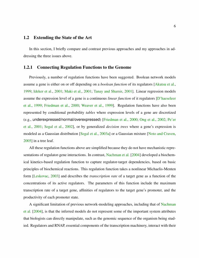
1.2.1 Connecting Regulation Functions to the Genome

Previously, a number of regulation functions have been suggested. Boolean network models

assume a gene is either on or off depending on a boolean function of its regulators [Akutsu et al.,

1999; Ideker et al., 2001; Maki et al., 2001; Tanay and Shamir, 2001]. Linear regression models

assume the expression level of a gene is a continuous linear function of it regulators [D’haeseleer

et al., 1999; Friedman et al., 2000; Weaver et al., 1999]. Regulation functions have also been

represented by conditional probability tables where expression levels of a gene are discretized

(e.g., underexpressed/normal/overexpressed) [Friedman et al., 2000; Ong et al., 2002; Pe’er

et al., 2001; Segal et al., 2002], or by generalized decision trees where a gene’s expression is

modeled as a Gaussian distribution [Segal et al., 2003a] or a Gaussian mixture [Noto and Craven,

2005] in a tree leaf.

All these regulation functions above are simplified because they do not have mechanistic repre-

sentations of regulator-gene interactions. In contrast, Nachman et al. [2004] developed a biochem-

ical kinetics-based regulation function to capture regulator-target dependencies, based on basic

principles of biochemical reactions. This regulation function takes a nonlinear Michaelis-Menten

form [Leskovac, 2003] and describes the transcription rate of a target gene as a function of the

concentrations of its active regulators. The parameters of this function include the maximum

transcription rate of a target gene, affinities of regulators to the target gene’s promoter, and the

productivity of each promoter state.

A significant limitation of previous network-modeling approaches, including that of Nachman

et al. [2004], is that the inferred models do not represent some of the important system attributes

that biologists can directly manipulate, such as the genomic sequence of the organism being stud-

ied. Regulators and RNAP, essential components of the transcription machinery, interact with their

7

binding sites in the genome in order to initiate transcription, and this initiation is often the key step

in producing mRNA molecules. However, most previous approaches do not model the binding of

regulators to their binding sites, and approaches that do consider binding events, such as Nachman

et al. [2004], do not explicitly account for features in the genome that affect regulator binding.

In contrast, my approach extends the previous state of the art by representing and learning the

key kinetic parameters in regulation functions that govern transcription rates as functions of fea-

tures in the genomic sequence. For example, the binding affinity of a given transcription factor to

the promoter regions in which it binds is represented as a function of the relevant DNA sequence

in the promoter regions, and the coefficients in this function are learned from sequence and ex-

pression data. This approach provides a more mechanistic representation of the regulator-gene

relationship. Therefore, it offers more explanatory power than alternative models. For example, it

can explain why a given kinetic parameter has the value it does and it enables one to predict how

certain changes in the genomic sequence might affect gene regulation.

1.2.2 Discovering Regulators

Besides representing and learning the parameters in regulation functions, gene regulatory-

network reconstruction includes another subtask: reconstructing the structure of the networks,

i.e., figuring out the connectivity between regulators and target genes.

Some previous approaches infer the connections between genes based on their observed mRNA

levels, and treat genes whose mRNA levels correlate with those of their connected target genes as

direct/indirect regulators (e.g., Friedman et al. [2000]). Some approaches assume a pre-defined

list of candidate regulators, so the network structure reconstruction boils down to determining the

connections between this list of regulators and genes in a model (e.g., Pe’er et al. [2002]; Segal

et al. [2003a]). These previous approaches do not consider the addition of currently unknown

(hidden) regulators that might be important for the cellular process being modeled.

A hidden regulator might be one whose corresponding gene is not discovered yet in an organ-

ism, or whose role is not characterized in the particular cellular process being studied. Moreover,

a hidden regulator may or may not be a protein molecule—it could be other DNA binding factors

8

such as protein-metabolite complexes that have not been experimentally detected before. Because

our knowledge of regulators and their target genes in a species or in a biochemical response is of-

ten incomplete, hidden regulator discovery is an important issue in gene regulatory-network recon-

struction. From the modeling point of view, this hidden regulator-discovery process corresponds

to network structure refinement.

Some existing methods have addressed this regulator-discovery subtask, such as Nachman et al.

[2004] and Noto and Craven [2005], by automatically adding new regulators when known regula-

tors cannot explain observed gene expression data. The drawback of these expression-data-based

approaches is that spurious regulators might be added into a network structure to “explain” the

noise in the expression data. That is, these approaches solely rely on using gene expression data to

propose hidden regulators; therefore such models are prone to fitting the noise in the data.

My approach to network structure refinement takes as input known regulator-gene relationships

from background knowledge and starts the regulator-discovery process when the existing regula-

tors cannot accurately explain the expression patterns of some genes. These weakly explained

genes are then clustered, and are further examined for common sequence features in their regu-

latory sequences. Hidden regulators are suggested only when shared sequence features are found

for a set of target genes. Hence, hidden regulators are proposed based on not only expression data

but also genomic sequences in my approach. In other words, I propose a hidden regulator when its

target genes have similar binding sites in their regulatory regions.

Although these common binding sites provide additional biological evidence to support exis-

tence of certain hidden regulators, the motif finding subtask is not trivial since these binding-site

signals are sometimes weak and motif finding tools may suggest spurious DNA motifs. Thus, I

have developed motif post-processing methods for filtering and ranking candidate motifs suggested

by motif finders in order to propose hidden regulators with high precision.

1.2.3 Handling Unmeasured Events

Many of the network reconstruction methods attempt to learn regulatory connections by model-

ing dependencies between the mRNA levels of a transcription factor and its target genes. In doing

9

this, however, they essentially ignore a whole set of regulation events, such as the translation of a

regulatory protein, activation of the protein, translocation of the protein, and binding of the pro-

tein to the promoter of a target gene. These processes are not measured in usual high-throughput

experiments, therefore their effects are essentially hidden from us.

It is well known that active regulators, not mRNA levels of the corresponding coding genes,

are what directly control the expression of target genes. Since most previous reconstruction meth-

ods do not consider the unmeasured events, they have to make some simplified assumptions. For

example, they use mRNA levels of genes as proxy for the activity levels of the corresponding pro-

teins. This is problematic as there are numerous examples showing that an activation or inhibition

of a regulator is conducted by post-transcriptional protein modifications.

Some previous methods have handled these unmeasured events by using hidden variables to

represent the activities/states of regulators [Battogtokh et al., 2002; Hartemink et al., 2001; Li et al.,

2006a; Liao et al., 2003; Nachman et al., 2004; Noto and Craven, 2005]. My approach also uses

hidden variables to represent regulator activity in order to encompass unmeasured events that occur

before regulators bind to promoter sequences [Pan et al., 2007].

1.3 Dissertation Motivation

As stated before, a significant limitation of previous approaches for reconstructing gene regula-

tory networks is that they do not directly address, in a quantitative way, the physical regulator-gene

interactions, and the genomic features that are involved in such interactions. The underlying mech-

anisms of transcription regulation tell us that regulators regulate gene expression by recognizing

and binding to the promoter regions of target genes to help or disable transcription initiation, which

is crucial in determining gene expression levels. Therefore, it makes sense to consider binding in-

teractions and the relevant regulatory sequences when inferring the parameters and structure of

regulatory-network models.

10

The machine-learning approaches in this dissertation consider genomic sequences, in addition

to gene expression data, in inferring the parameters of kinetics-based regulatory network mod-

els, and in refining the network structure given a prior network model structure. Such sequence-

based approaches extend the state-of-the-art of parameter and structure learning in gene regulatory-

network reconstruction. The primary motivations of my approaches are:

• provide a more mechanistic representation of the regulatory relationships being modeled;

• explain observed gene expression phenomena in terms of causality rather than correlation

(i.e., distinguish regulation from coexpression);

• predict likely effects of genetic perturbations on gene regulation;

• suggest potential hidden regulators that are supported not only by microarray data but also

sequence evidence to assist biologists in discovering new regulatory relationships.

1.4 Dissertation Statement

This thesis aims to answer several questions with regard to reconstructing gene regulatory

networks. Specifically, I focus on the following hypotheses:

i Models that represent and learn the key kinetic parameters as functions of features in the

genomic sequence offer more explanatory power and biological insight than models that do

not.

ii Models that include sequence-based kinetic parameters provide predictive accuracy that is

better than similar models without sequence-based parameters.

iii Models that consider both gene expression data and genomic sequences can propose hidden

regulators with high precision.

iv Post-processing candidate DNA motifs suggested by motif finders can help identify true

regulator binding sites more accurately than when post-processing is not performed.

11

1.5 Dissertation Outline

This dissertation stands at the intersection of computer science, statistics and molecular biol-

ogy. However, it does not assume that readers have solid background in the above areas. The

remainder of this dissertation is organized as follows:

• Chapter 2 presents background information about the relevant biological concepts and tech-

niques as well as computational models and methods.

• Chapter 3 discusses some of the previous work that is related to my approaches. It serves as

a brief literature review on four relevant research topics. It also compares and contrasts the

methods presented in Chapter 4 and Chapter 5 with previous state-of-the-art ones.

• Chapter 4 presents a method for connecting quantitative regulatory network models to the

genome. This genome sequence-based modeling approach can help biologists better under-

stand observed gene regulation phenomena and make gene expression predictions.

• Chapter 5 proposes a novel framework for discovering hidden regulators in gene regulatory

networks. This framework’s pipeline takes as input high-throughput gene expression data

and genomic sequences, along with background knowledge of regulator-gene relationships,

and then automatically outputs biologically interpretable hypotheses regarding likely hidden

regulators in cellular processes being modeled.

• Chapter 6 describes my additional research in learning Bayesian network models for breast

cancer prediction, a task not directly related to inferring gene regulatory network models.

• Chapter 7 summarizes the key contributions of this dissertation, proposes future work in

reconstructing gene regulatory networks, and draws some concluding remarks.

12

Chapter 2

Background

This chapter provides background information that is necessary to understand the remainder

of this dissertation. I begin with fundamental biological concepts in gene regulation and the tech-

niques used to measure gene expression. I then describe the important computational concepts

necessary to understand my approach to studying gene regulatory networks.

2.1 Biological Concepts and Techniques

This section offers a brief overview of some basic biological concepts of molecular biology

relevant to gene regulation. Interested readers are referred to general molecular biology textbooks

for more information (e.g., Lodish et al. [2007]).

2.1.1 Gene Regulation

Cells are the fundamental working units of every living system. According to the Central

Dogma of molecular biology, shown in Figure 2.1, DNA, RNA and protein are the three important

entities in living cells, and genetic information flows from DNA through RNA to protein1. DNA

is a nucleic acid that contains the genetic instructions specifying the biological development of all

cellular forms of life. Four nucleotides, denoted as A, C, G and T, make up the double-stranded

DNA molecules.

RNA, which usually is a single-stranded nucleic acid, is transcribed from a region on the DNA

molecule, called a gene, by enzymes called RNA polymerases (RNAPs) through a process known

1There are some exceptions to this information flow, such as the reverse transcription in some viruses where geneticinformation can flow from RNA to DNA.

13

The Central Dogma of Molecular Biology

ReplicationDNA duplicates

TranscriptionRNA synthesis

TranslationProtein synthesis

DNA

Information

Information

mRNA

RNA polymerase Nucleus

Cytoplasm

Nuclear membrane

mRNAribosome

protein

Protein

RNA

(Andy Vierstraete 1999)

Figure 2.1: The central dogma of molecular biology. DNA replicates its information in a processcalled replication. Genetic information flows from DNA to RNA by the transcriptionprocess and from RNA to protein by the translation process. This figure is fromhttp://users.ugent.be/~avierstr/principles/centraldogma.html.

14

as transcription. In some organisms such as bacteria, a single RNA molecule can be transcribed

from several contiguous genes. A set of genes transcribed into a single RNA molecule is known as

an operon. One type of RNA molecule, called messenger RNA2 (mRNA), serves as templates for

complexes called ribosomes to synthesize corresponding proteins, in a process termed translation.

The structure and activity of a protein can be changed by a post-translational modification process.

Proteins, chains of amino acids, are essential to the structure of all living cells and perform a wide

variety of biological functions.

The quantities of RNA and protein molecules and their activity states are both subject to regu-

lation occurring at different stages of the above process. The differences in regulation of various

genes, and under different conditions, create the variety and dynamics of cells. Although any

step of gene regulation may be modulated (from the DNA→ RNA transcription step to the post-

translational modification of a protein), transcription regulation generally plays a key role in this

process as it is the first and crucial step to regulate gene expression. Gene expression, in a broad

sense, is the whole process by which information from a gene is used in the synthesis of a functional

gene product (a protein or RNA). However, in a strict sense and this dissertation, gene expression

means the process of creating RNA molecules. Note that, for a given gene, the total amount of its

mRNA is regulated not only by the expression (creation) of mRNA, but also by the degradation

(decay) of mRNA.

Transcription regulation can be negative or positive. In negative regulation, a repressor protein

binds to the DNA sequence upstream of a gene called promoter and inhibits transcription. In posi-

tive regulation, an activator interacts with the RNAP in the promoter region to initiate transcription.

These repressor and activator proteins are commonly called transcription factors or TFs for short.

The exact TF binding sites in promoter sequences tend to be short DNA subsequences and are

termed transcription factor binding sites (TFBSs). Transcription factors often work together in

different combinations, to ensure the correct amount of each gene is transcribed.

Transcription factors are themselves proteins so they are subject to transcriptional regulation

as well. Many transcription factors are also heavily regulated by post-translational modifications

2Other types of RNA include transfer RNA (tRNA), ribosomal RNA (rRNA) and microRNA (miRNA), etc.

15

such as phosphorylation to dynamically induce or inhibit their protein activity (i.e., to regulate the

activated protein level). Figure 2.2 illustrates the relationships between the mRNA level, protein

level and protein activity of a transcription factor by showing a regulatory path between a tran-

scription factor and a target gene; it also emphasizes some cellular quantities that can or cannot be

measured by expression profiling techniques (to be explained in Section 2.1.2).

In addition to regulatory proteins like transcription factors, RNA molecules such as microRNAs

(miRNAs) in plants and animals, and antisense RNAs in bacteria can also affect gene regulation

in cells. Thus, a regulator is not necessarily a protein; it can be a RNA molecule or other cellular

entity.

The interactions between various proteins, genes, and other cellular molecules form very com-

plex “biological circuits” even in lower organisms such as bacteria. Gene regulatory networks3

(GRNs) are one type of such “circuits”. Broadly speaking, a typical GRN consists of input signal-

ing pathways, regulatory proteins that integrate the input signals, target genes (or target operons in

bacteria), and the RNA and proteins produced from these target genes. In addition, these networks

may include dynamic feedback loops that can further regulate gene expression. Figure 2.3 shows

an example of a gene regulatory network and illustrates several basic properties of the network.

However, strictly speaking, the relay of signals from outside a cell to the genetic sequences of

a cell is the main functionality of another type of “biological circuit” called signaling networks.

These signaling networks describe interactions among various proteins and/or small molecules

that propagate extracellular signals inside the cell. Since cellular networks are linked together, the

boundaries between gene regulatory networks and signaling networks are often not clear. To be

precise, in this dissertation, I focus on the regulator-gene interactions that control the expression

of particular genes. That is, I study/explore which regulators control a gene and the regulatory

functions that gene expression depends on. Such a research task is often called gene regulatory

networks modeling/reconstruction/inference. These three alternative words are sometimes used

interchangeably for this task in literature and this dissertation.

3Gene regulatory networks are also called gene networks, regulatory networks, genetic regulatory networks, regu-latory pathways or transcriptional networks.

16

ActiveProtein T

mRNA G

Protein TmRNA T

TranscribedmRNA G

DegradedmRNA GObserved Hidden

Activation signal

Activation of gene G’s transcription

Degradation of mRNA G

Translation

Remaining mRNA G

Figure 2.2: Illustration of a regulatory path between a transcription factor T and a target gene G.The mRNA encoding the transcription factor (mRNA T) is translated to protein T(green oval). This protein is activated (pink oval) and induces the transcription of thetarget gene G at a certain rate. The final accumulation of mRNA G levels is deter-mined by the transcribed mRNA G and by the degradation of mRNA G. Each ofthe ovals is associated with a relevant quantity (mRNA T level, protein T level, ac-tivated protein T level, target gene transcribed mRNA G level, degraded mRNAG level and the remaining mRNA G level). A microarray experiment only measuresthe first and last of these quantities (Observed), whereas the other quantities are not ob-served (Hidden). The blue arrow indicates the most relevant quantities on this path betweenthe transcription factor T and the target gene G.

17

Figure 2.3: An example of a gene regulatory network. In this example, two different signalsimpinge on a single target gene where the cis-regulatory elements provide for an in-tegrated output in response to the two inputs (a cis-regulatory element is a region ofDNA or RNA that regulates the expression of genes located on that same strand). Sig-nal A triggers the conversion of inactive transcription factor A into an active formthat binds directly to the target gene’s cis-regulatory sequence. The process for signalB is more complex. Signal B triggers the separation of inactive transcription factorB (brown oval) from an inhibitory factor (yellow rectangle). TF B is then free to forman active complex that binds to the cis-regulatory sequence as well. The net outputis expression of the target gene at a level determined by the action of transcriptionfactors A and B. In this way, cis-regulatory DNA sequences, together with the tran-scription factors that assemble on them, integrate information from multiple signalinginputs to produce an appropriately regulated gene-expression output, e.g., mRNA andprotein molecules. A more realistic network might contain multiple target genes reg-ulated by signal A alone, others by signal B alone, and still others by the pair ofsignal A and B. This figure is courtesy of U.S. Department of Energy Genomes toLife Program, http://doegenomestolife.org.

18

2.1.2 Experimental Techniques

In order to study the structures and mechanisms of gene regulation, we need experimental tech-

niques to measure the components and products of regulatory paths at various steps. In particular,

we want to measure the quantities of mRNA and protein produced for genes of interest, i.e., the

“expression levels” of mRNA and protein for specific genes.

Traditionally, these measurements were performed at the level of a few individual genes at a

time by experimental biologists, which is a time-consuming and labor-intensive process. Genomic

technology breakthroughs introduced methods which can simultaneously measure mRNA expres-

sion levels for many hundreds and even thousands of genes. These high-throughput assays which

can probe cells at a genome-wide scale are based on the inventions of DNA microarrays [Schena

et al., 1995]. DNA microarray consists of thousands or more probes, either oligonucleotides or

complementary DNAs (cDNAs), that are affixed on a solid organized surface. These probes can

be used to detect RNA transcript amounts, therefore providing quantitative measurements of gene

transcription. As an example, Figure 2.4 shows how microarray technology is applied to detecting

gene differential expression in tumor cells.

Although the use of microarrays is currently the most common method to measure RNA con-

centrations in a high-throughput fashion, microarray measurements are subject to noise such as

nonspecific cross hybridization [Aris et al., 2004]. Other techniques such as RNA-seq [Wang

et al., 2009], SAGE [Velculescu et al., 1995] and SuperSAGE [Matsumura et al., 2003] are more

accurate since they sequence individual RNAs. These more accurate technologies will become

more common as their cost becomes lower.

Methods for measuring protein levels in high-throughput fashion have also been developed

[Haynes and Yates, 2000], but the availability of large scale data sets is much more limited; and I

do not have such protein-measurement data sets in my study.

These high-throughput techniques, along with other methods (e.g., DNA sequencing, ChIP-

chip) in biology have generated a large amount of data that can potentially provide genome-level

information regarding the underlying structure, dynamics and mechanisms of gene regulation.

19

Figure 2.4: An example application of microarray technology. Microarray technology allows thesimultaneous examination of tens of thousands of genes through the use of slidesor chips. In this example, it involves extracting all messenger RNA from the tumorcells, converting it to its complementary DNA (cDNA) through the RT/PCR process,labeling it with a fluorescent dye, and applying it to a microarray. DNA moleculesbind/hybridize to their corresponding genes on the array. The same procedure is doneto a “normal” group of cells, but with a different color of fluorescent dye. A laser scansthe microarray and analyzes the intensity of the different colors to give expressioninformation on each gene. For example, a spot on the microarray turns red if thecorresponding gene is highly expressed in the tumor cells but not in the “normal”cells; it turns green if the corresponding gene is highly expressed in the “normal”cells but not in the tumor cells. This figure is from http://www.genome.gov.

20

2.2 Computational Models and Methods

I now shift gears to review some main computational concepts that are important for under-

standing my work, including Bayesian networks, expression clustering and motif discovery.

2.2.1 Bayesian Networks

Bayesian networks provide a language for compactly representing joint probability distribu-

tions of random variables. Bayesian networks have been applied extensively to modeling complex

domains in many different fields [Heckerman et al., 1995]. One important ingredient for many

applications is the ability to induce such models from data. This is especially important when the

knowledge about the domain is partial, as is the case in the biological domains addressed in this

dissertation. I now give a brief overview of the formalism of Bayesian networks and the types

of learning tasks involved in inducing such models from data. Some parts of the material in this

section were also presented in Pe’er [2003].

Let us consider a finite set X = {X1, . . . , XN} of random variables. Each variable Xi may

be discrete, in which it may have any value xi from the domain of all possible values of Xi, or it

may be continuous, in which case it may take a value from some real interval. I use capital letters

such as X, Y, Z for variable names and lowercase letters x, y, z for specific values taken by these

variables. Sets of variables are denoted by boldface capital letters X,Y,Z.

Before I describe Bayesian networks, I need to cover three probability concepts, namely joint

probability, conditional probability and the product rule, using an example of two variables (X = x

and Y = y) as follows. The joint probability of X = x and Y = y is denoted by

P (x, y) ≡ P (X = x ∧ Y = y),

and the conditional probability of X = x given Y = y is denoted by

P (x | y) ≡ P (X = x | Y = y),

and they are related as shown in the probability product rule:

P (x, y) = P (x | y)P (y) = P (y | x)P (x).

21

The generalization of product rule is the chain rule of probabilities:

P (X1, . . . , XN) = P (X1 | X2, . . . , XN)P (X2 | X3, . . . , XN) . . . P (XN−1 | XN)P (XN).

An important concept in Bayesian networks is conditional independence: X is conditionally

independent of Y given Z if

P (X|Y,Z) = P (X|Z).

This independence statement is denoted by (X ⊥ Y | Z). Figure 2.5 illustrates such conditional

independence in a simple Bayesian network.

Formally, a Bayesian network (BN) [Pearl, 1988] is a representation of a joint probability dis-

tribution over a set of random variables. It consists of two components:

• A directed acyclic graph (DAG), G, whose vertices (i.e., nodes) correspond to the random

variables X = X1, . . . , XN , and whose edges (i.e., links) indicate dependence relationships

over X (i.e., whose missing edges indicate conditional independencies between the vari-

ables).

• A set of conditional probability distributions (CPDs), θ, describing the distribution for each

variable Xi in X given its parents in the graph.

In other words, G gives a set of independence conditions between variables and θ gives a local

probability model for each variable given its parents in the network. Together, these two com-

ponents, G and θ, specify a unique distribution over X = X1, . . . , XN . As a direct consequence

of the chain rule of probabilities and properties of conditional independence, the joint probability

over X can be written as

P (X1, . . . , XN) =n∏i=1

P (Xi | Ui),

where Ui represents the parent nodes of the variable Xi in G. This product form describes why a

Bayesian network represents a compact joint probability distribution. For example, let us consider

again the five variables in Figure 2.5. Without using any independence assumptions, the joint

probability distribution can be written as:

P (A,B,C,D,E) = P (E|A,B,C,D)P (D|A,B,C)P (C|A,B)P (B|A)P (A).

22

E A

B D

C

Figure 2.5: Conditional independence in a simple Bayesian network. This network structure im-plies several conditional independence cases: (A ⊥ E), (B ⊥ D | A,E), (C ⊥A,D,E | B), (D ⊥ B,C,E | A), and (E ⊥ A,D).

In contrast, using the independence assumptions implied by the network in Figure 2.5, the same

distribution can be expressed as:

P (A,B,C,D,E) = P (E)P (A)P (B|A,E)P (D|A)P (C|B).

If the variables are all binary in this network, the former form requires 31 parameters, while the

latter only needs 10 parameters. More generally, if G is defined over N binary variables and their

maximal number of parents is bound byM , then instead of using 2N−1 independent parameters to

represent the full joint probability distribution, a Bayesian network model can represent the same

joint distribution with at most 2MN parameters.

I have described the structure part of a Bayesian network, so next I discuss the parameterization

of the conditional probability distributions (CPDs), i.e., P (Xi | Ui). A CPD can be thought as an

input-output “device” in a node that takes as input the values of parent nodes and outputs the

probability of seeing a particular value of this node. That is, a CPD is a function that outputs a

distribution of a variable using that variable’s parent values as the input. This function can be of any

general form. When both a variable Xi and its parents Ui are discrete, a common representation

for a CPD is a conditional probability table (CPT). Each row in the table corresponds to a specific

23

joint assignment uXito Ui, and specifies the probability distribution for Xi conditioned on uXi

.

Therefore, if uXiconsists of m binary variables, then the table will specify 2m distributions. For

example, assuming variables A,B,E in Figure 2.5 are all binary, the CPT for the variable B might

look like:

A E P (b = 0) P (b = 1)

0 0 0.9 0.1

0 1 0.7 0.3

1 0 0.5 0.5

1 1 0.2 0.8

Such a table representation is general enough to describe any discrete conditional distribution.

When a variable and some or all of it parents are real-valued (i.e., continuous variables), there

is no general form to represent all types of dependence. For cases where all the parents are contin-

uous, the linear Gaussian function is one widely used probability distribution representation:

P (X | U) ∼ N(a0 +∑j

ajU[j], σ2).

Here, X is normally distributed around a mean that linearly depends on the values of its parents; aj

is the coefficient for parent j; U[j] is the value of parent j. The variance of this normal distribution

is not dependent on its parents’ values. So the total number of parameters is |U| + 2: |U| + 1

linear coefficients and one variance parameter. Note that, compared to the CPT representation

of multinomial distributions, the number of parameters is typically much smaller in continuous

variable CPDs. Besides the linear Gaussian function, non-linear function forms have been used

to model non-linear dependence, such as the sigmoid function [Bishop, 1995] and the Michaelis-

Menten saturation function [Nachman et al., 2004].

As has been stated, a major advantage of Bayesian network models is the ability to learn them

from observed data. That is, given a series of observed events described by a set of random vari-

ables, a Bayesian network model can be learned to characterize the relationships among these

24

variables. This is important for the gene regulation domain addressed in this dissertation because

we often do not know the (complete) picture of the structure and parameters of a gene regulatory

network. The learning process may involve two subtasks: learning the structure of the BN—

recovering the directed graph, i.e., G; and learning the parameters of the BN—assigning values to

the parameters of the CPDs, i.e., θ. A more challenging subtask is to also simultaneously deter-

mine if the events can be better explained or modeled by latent variables (hidden variables). That

is, beyond finding the right connectivity among pre-existing nodes, this task entails discovering or

inventing additional relevant variables that are not in the input set of random variables. In practice,

a Bayesian network learning task may involve parameter learning only, parameter and structure

learning without hidden variables, or with hidden variables, etc.

When applying Bayesian networks to genetic regulatory systems, vertices can be used to rep-

resent expression levels of genes and activity levels of regulators; edges can indicate the existence

of interactions among genes and regulators. The conditional probability distributions characterize

these interactions as input-output pairs, e.g., the expression of a gene is dependent on the activity of

its regulators. Hidden variables might correspond to genes or regulators that are not included in the

current knowledge. This dissertation involves modeling gene regulatory networks using Bayesian

networks. The details of parameter learning and structure learning are described in Chapter 4 and

Chapter 5, respectively.

2.2.2 Gene Expression Clustering

The goal of clustering is to divide a set of items in such a way that similar items fall into the

same cluster, while dissimilar items group in distinct clusters. Many clustering methods have been

developed outside the biology field; here I describe their features and applications in the context

of gene expression analysis.

Gene expression clustering allows subdividing thousands or even more genes into a smaller

number of categories. It is often one of the first steps in gene expression analysis. The resulting

clusters can be used for downstream exploration of data. For example, a gene cluster of similar

expression patterns could be used to identify potential regulatory binding sites in the promoters of

25

these genes; a gene cluster could also help infer the cellular roles of genes of unknown function in

the same cluster.

The first choice that must be made in gene expression clustering is to define the similarity

measure (alternatively, distance) between gene expression profiles. The expression profile of a gene

refers to the expression values for that gene across some experimental conditions, or across some

time points for a time-series measurement. There are many ways to compute the similarity between

two series of numbers (e.g., expression values). The most commonly used similarity measure is

probably the Pearson correlation. If you plot two series of numbers as two separated curves, then

the Pearson correlation basically tells you how similar the shapes of two curves are. The Pearson

correlation coefficient is always between −1 and 1, with 1 meaning the two series of numbers are

of increasing linear relationship,−1 meaning decreasing linear relationship, 0 meaning completely

uncorrelated. Pearson correlation is invariant under linear transformations of the data; therefore

two curves that have the identical shape, but different magnitude, have a correlation of 1. The

Pearson correlation has some variants. For example, uncentered correlation assumes the mean of

a series of numbers is 0. This uncentered correlation is equal to the cosine of the angle of two

n-dimensional vectors. Another variant is the Spearman rank correlation, which is essentially the

non-parametric version of the Pearson correlation. Spearman rank correlation replaces the data

values in a series of numbers with the ranks of these numbers in the series; therefore it is more

robust against outliers (at the cost of some information loss). These correlation-based similarity

measures are summarized in Table 2.1, along with two non-correlation-based measures. They are

also discussed in D’haeseleer [2005].

For some clustering methods, another choice must also be made regarding the intercluster

similarity (or distance), i.e., the linkage function. Some commonly used ones are complete linkage

(the distance between two clusters is the largest distance between any two members of the clusters),

average linkage (average distance between any two members), single linkage (shortest distance

between any two members), and centroid linkage (distance between the two cluster centroids).

Due to such a wide variety of similarity criteria and the methods to cluster genes (or subclusters

of genes), there are a lot of clustering algorithms available for gene expression clustering. Two

26

Table 2.1: Gene expression similarity and distance measures. dfg is the distance between expres-sion patterns for genes f and g; rfg is the correlation between expression patterns forgenes f and g; egc is the expression level of gene g under condition c; eg is the averageexpression values of gene g across all conditions.

Measure Formula

Manhattan distance dfg =∑

c |efc − egc|

Euclidean distance dfg =√∑

c(efc − egc)2

Uncentered correlation rfg =

∑c efcegc√∑c e

2fc

∑c e

2gc

Pearson correlation rfg =

∑c(efc − ef )(egc − eg)√∑

c(efc − ef )2∑

c(egc − eg)2

Spearman rank correlation As Pearson correlation, but replace egc with

the rank of egc within the expression values

of gene g across all conditions c = 1 . . . C

common classes of gene expression clustering methods are hierarchical clustering and partitioning.

The basic idea of hierarchical clustering is to either iteratively divide a root cluster containing all

genes into smaller subclusters (top-down fashion) until single-gene clusters are generated, or start

with single-gene clusters and successively join the most similar clusters until all genes are joined

into one supercluster (bottom-up fashion). In both cases, a tree-shaped data structure is formed;

a horizontal cut is typically executed to induce a certain number of final clusters. Partitioning

27

methods, in contrast, divide data into what is a usually pre-defined number of subsets without

constructing hierarchical relationships between these subsets. When the number of true clusters in

the data is not known, repeatedly running the algorithm with different numbers of clusters is often

conducted to search for the optimal number of clusters.

Figure 2.6 shows a gene-expression clustering example using hierarchical clustering, k-means

(a partitioning clustering method) and another popular method called self organizing map (SOM).

Besides these three methods, other clustering algorithms are also discussed in Chapter 3.

As shown in Figure 2.6, clustering results can be different depending on the applied clustering

methods. The quality of these clustering results can be evaluated based on internal or external cri-

teria. Internal criteria are concerned with the statistical properties of the clusters; external criteria

are related to additional information that was not used in the clustering process.

It may seem easy to use internal criteria such as the compactness and separation of clusters;

however there is no single consensus of what “good” clustering should look like—a good clustering

might optimize the variance of clusters, minimize the radius of clusters, emphasize the stability of

clusters with respect to noise, etc.

The more reliable quality measure of a clustering method on a gene expression data set is to

assess its clustering performance based on the biological information that is not used during the

clustering process itself. For example, if the goal is to cluster genes with similar functions, then

one can use known functional annotations to judge a clustering algorithm. Unfortunately, such

prior knowledge may not be available (or adequate) for a particular gene expression clustering

task, especially for an open-ended exploration of a not well-studied organism.

Finally, note that gene expression clustering can be gene-based (clustering genes showing pat-

terns across samples), sample-based (clustering samples showing patterns across genes), or both.

The work in this dissertation focuses exclusively on gene-based clustering.

28

Figure 2.6: A simple clustering example with 40 genes measured under two different conditions.(a) The data set contains four clusters of different sizes, shapes and numbers of genes.Left: each dot represents a gene, plotted against its expression value under the twoexperimental conditions. Euclidean distance, which corresponds to the straight-linedistance between points in this graph, was used for clustering. Right: the standard red-green representation of the data and corresponding cluster identities. (b) Hierarchicalclustering finds an entire hierarchy of clusters. The tree was cut at the level indicatedto yield four clusters. Some of the superclusters and subclusters are illustrated on theleft. (c) k-means (with k = 4) partitions the space into four subspaces, depending onwhich of the four cluster centroids (stars) is closest. (d) SOM finds clusters, whichare organized into a grid structure (in this case a simple 2 × 2 grid). This figure isfrom D’haeseleer [2005].

29

2.2.3 Motif Discovery

As stated in Section 2.1.1, gene expression starts with binding of regulatory factors, such as

transcription factors, to the regulatory sequences of genes, such as their promoters. These reg-

ulators control gene expression by either activating or repressing the transcriptional machinery.

Identifying the binding sites in DNA sequences for regulators is a key task in understanding gene

regulation mechanisms. Since the binding sites of a regulator often share some sequence regu-

larity, the task boils down to finding an unknown pattern that occurs frequently in a given set of

sequences.

A DNA motif is defined as a nucleotide sequence pattern that has some biological role such as

acting as a binding site for a transcription factor. A particular binding site of a regulator is often

called an “occurrence” of the DNA motif. Since DNA binding sites of a given regulator are usually

not exactly the same from instance to instance, having varying degrees of affinity for the regulator,

they are typically represented by position specific probability matrices (PSPM). Position specific

probability matrices are also often graphically depicted using sequence logos. A PSPM represents

a motif as a fixed-length sequence of base (nucleotide) distributions; i.e., it provides information

on the probability of each base at each position of the corresponding motif. Such information

can be interpreted by information theory to generate corresponding graphical representation—the

sequence logo. Figure 2.7 shows an example of a PSPM and the corresponding sequence logo.

Furthermore, a PSPM can be transformed into a position weight matrix (PWM), which can be used

to score a sequence of the same length as the PWM to measure how close that sequence would

match the pattern described by the PWM [Hertz and Stormo, 1999].

Now that I have described the definition of a motif and its representations, the task of computa-

tional motif discovery (or motif finding) can be defined as follows: given a collection of sequences

that are believed to contain a regulator’s unknown binding sites, find this regulator’s binding sites

in these sequences de novo and induce a motif from these sites. In practice, the induced motif is

often represented by a PSPM or a sequence logo.

Motif discovery can be viewed as a “needle in a haystack” problem [Bailey et al., 2006]. That

is, a motif discovery algorithm looks for a set of similar short sequences (the needle) in a set of

30

Position: 1 2 3 4 5 6 7 8 9A .1 .4 .1 .8 .0 .2 .0 .1 .0C .0 .0 .0 .2 .5 .0 .1 .7 .5G .0 .4 .7 .0 .0 .8 .0 .2 .0T .9 .2 .2 .0 .5 .0 .9 .0 .5

Figure 2.7: An example of a 9-base-wide position specific probability matrix (PSPM). The baseat each position, 1-9, is assumed to come from an independent distribution over{A,C,G,T}. Shown below the matrix is the logo representation of the same dis-tribution. The information content (in terms of bits) of each position is represented bythe height of the letters (information content is described in Chapter 5). The taller theletter, the more likely it is at that position.

much longer sequences (the haystack). This problem is easier when the motif instances are long

and very similar to each other. But it gets much harder when the motif occurrences are short and/or

degenerate, or the input sequences are very long.

A large number of motif discovery algorithms have been developed. Many of them are grouped

and briefly discussed in Chapter 3. Here I describe some properties of two motif finding algorithms,

MEME and PhyloCon, since they are employed as the important plug-in methods in my work. The

reasons for choosing these two motif discovery methods are also explained in Chapter 3.

MEME (Multiple EM for Motif Elicitation) is one of the most widely used tools for discovering

motifs in a set of DNA or protein sequences [Bailey and Elkan, 1994]. MEME uses a process akin

to gapless, local, multiple sequence alignment to search for statistically significant motifs in the

input sequence set. Each input sequence is allowed to contain zero, one, or more motifs. Thus the

31

algorithm is capable of discovering several different motifs with different number of occurrences

in a given data set. MEME chooses the width of each motif automatically in order to minimize the

E-value of the motif, i.e., the probability of finding an equally well-conserved pattern in random

sequences.

PhyloCon is a algorithm that takes into account both conservation among orthologous genes

and co-regulation of genes within a species to improve the ability to identify motifs [Wang and

Stormo, 2003]. Orthologous genes (orthologs) are genes in different species that are similar to each

other because they originated from a common ancestor. The benefit of considering orthologous

genes in motif discovery is based on the assumption that regulatory elements (e.g., transcription

factor binding sites) in non-coding regions are under a higher selective pressure during evolution

than non-functional regions. Therefore aligning orthologous regions from two or more organisms

should highlight the conserved parts which are expected to play a functional role, e.g., interact with

TFs [Tagle et al., 1988]. The PhyloCon algorithm first aligns conserved regions of orthologous

genes into multiple sequence alignments (i.e., profiles), then compares profiles representing non-

orthologous sequences. Motifs emerge as common regions in these profiles. Figure 2.8 sketches

out how PhyloCon works with a simple example.

2.3 Summary

In this chapter I have reviewed the important background knowledge to understand this dis-

sertation from two disciplines: biology and computer science. First, I covered relevant biological

concepts and techniques, including the central dogma of molecular biology, various gene regula-

tion mechanisms, properties of gene regulatory networks and microarray technologies. Second, I

explained some existing computational concepts and models involved in my approach to studying

gene regulatory networks. In particular, Bayesian networks represent a joint probability distribu-

tion over random variables and are suitable for modeling regulatory networks from gene expression

data; gene expression clustering aims to group functional related genes together; motif discovery

seeks to infer unknown regulatory elements from a collection of biological sequences. The basics

32

Figure 2.8: How PhyloCon works. (A) A diagram of how PhyloCon organizes and processesdata. Sequences are grouped based on orthology. Many initial profiles are generatedfor conserved regions. Comparison of profiles from different orthologous groups re-veals common motifs. (B) Alignments of orthologous sequences of four yeast speciesshow high conservation in the 5’UTR of three genes. Asterisks indicate positionswhere at least three out of four letters are identical. Conservation extends beyond thetrue motifs (LEU3), making it difficult to identify the motif by simply examining thephylogenetic relationship. However, the motif emerges after comparing profiles fromdifferent orthologous groups. This figure is from Wang and Stormo [2003].

33

of these computational models and methods have been covered in this chapter; related work will

be presented in the next chapter (Chapter 3).

34

Chapter 3

Related Work

In this chapter I describe some of the previous work that relates to my approach to learning

kinetic parameters in regulatory network models detailed in Chapter 4, and my approach to dis-

covering hidden regulators of genetic regulatory networks elaborated in Chapter 5.

These related methods fall into four research topics; therefore I discuss them in four inde-

pendent sections. Specifically, regulatory network modeling methods discussed in Section 3.1

are related to my work in both Chapter 4 and Chapter 5; gene expression clustering methods in

Section 3.2, motif discovery methods in Section 3.3, and motif filtering and ranking methods in

Section 3.4 are related to the corresponding modules in my approach presented in Chapter 5. The

goal of this chapter is threefold:

• First, it largely serves as a compact literature review of the early and state-of-the-art methods

that are related to my approaches.

• Second, it briefly compares my network modeling method and motif filtering and ranking

methods with the state-of-the-art ones; it also concisely explains why I adapt particular clus-

tering and motif-finding methods in my approaches.

• Third, it purposely helps reduce the length and burden of Chapter 4 and Chapter 5 by group-

ing the related work here; the breadth of the previous methods warrants this single chapter

as well.

35

3.1 Regulatory Network Modeling Methods

Various methods have been reported to reconstruct genetic regulatory networks from high-

throughput experimental data, such as genomic sequences, expression profiles and transcription

factor binding-site assays. A wealth of biological information from the literature and on-line

databases has been used for such reconstructions as well. Recall from Chapter 2 that genes can be

regulated by regulatory proteins (such as transcription factors), RNAs, or even protein-metabolite

complexes, etc. Since most methods to date study gene-gene or TF-gene relationships in gene reg-

ulatory networks, the discussion in this section assumes that regulators are transcription factors

unless otherwise specified. A complete review of each method is out of the scope of this chap-

ter, so I briefly present representative methods, then compare and contrast these methods from a

few different angles, and finally point out the key differences between my approach and previous

methods in brief.

3.1.1 Model Representation

A wide variety of model representations have been developed for modeling gene regulatory

networks.

• Boolean network models represent the state of a gene as a Boolean variable (on/off) and

interactions between genes as Boolean functions, which determine the state of a gene on the

basis of the states of some other genes [Akutsu et al., 1999, 2000; Ideker et al., 2001; Maki

et al., 2001; Tanay and Shamir, 2001]. Thus, Boolean network models make a simplistic as-

sumption about the possible expression levels most genes have. As discussed in Lahdesmaki

et al. [2003], Boolean network models also often implicitly assume noise-free measurements

of gene expression, i.e., uncertainty is not modeled by them.

• Differential equation models encode a gene network as a system of differential equations

[Chen et al., 1999; de Hoon et al., 2003; Li et al., 2008]. The rate of change in concentration

of a particular transcript is given by an influence function of other RNA concentrations.

Unless they are restricted to simple function forms, differential equation models involve a

36

large number of parameters—O(d2) parameters where d is the number of genes modeled

[Chan et al., 2007]. Moreover, differential equation models require time-series data to learn

the parameters.

• Weight matrix models represent regulatory relationships between genes as linear coefficients

in logistic functions, with the net influence on a gene’s expression being the summation of the

independent regulatory inputs [Weaver et al., 1999]. The main limitations of this approach

are that it assumes knowledge of maximal gene-expression levels, and is very sensitive to

noisy data.

• Relevance network models compute mutual information between RNA expression patterns

for each pair of genes, and then generate networks of gene-gene interactions [Butte and Ko-

hane, 2000]. The assumption is that an association with high mutual information means that

one gene is non-randomly associated with another; therefore the two are related biologically.

Butte and Kohane discretized expression values in order to calculate the mutual information

between genes, which may cause information loss.

• Petri nets are directed bipartite graphs for modeling and reasoning about concurrent, dis-

tributed systems [Reisig, 1985]. Petri net models and their relatives have been used to inves-

tigate the structure and dynamic behavior of genetic regulatory networks [Chaouiya et al.,

2004; Comet et al., 2005; Matsuno et al., 2000; Steggles et al., 2007]. However, an impor-

tant limitation of this modeling approach is that Petri net models are often developed by

a human-based trial and error approach that is time consuming and difficult; therefore this

modeling approach is likely to be infeasible as the complexity of the models increases.

• Bayesian network models are graphical representations of joint probability over random

variables [Pearl, 1988]. Bayesian networks can capture linear, non-linear, combinatorial,

stochastic and other types of relationships among variables. They are suitable for modeling

gene networks because of their ability to represent stochastic events, to describe locally in-

teracting processes, to handle noisy or missing biological data in a principled statistical way,

37

and to possibly make causal inferences from the derived models. The hidden variables in

Bayesian network models also provide a natural representation to account for the unobserved

levels of cellular components (e.g., activity levels of transcription factors) and the unmea-

sured biological processes (e.g., protein phosphorylation and degradation). Hence, Bayesian

networks, including their variants Dynamic Bayesian networks, Gaussian networks, Module

networks, mixture Bayesian networks and state-space models (SSMs), etc., have become

widely used tools for regulatory-network modeling [Armaanzas et al., 2008; Beal et al.,

2005; Chen et al., 2006; Djebbari and Quackenbush, 2008; Dojer et al., 2006; Friedman

et al., 2000; Grzegorczyk et al., 2008; Hartemink et al., 2001, 2002; Imoto et al., 2002,

2004; Kim et al., 2004; Ko et al., 2009; Li et al., 2006a,b; Murphy and Mian, 1999; Nach-

man et al., 2004; Nariai et al., 2005; Noto and Craven, 2005; Ong et al., 2002; Pe’er et al.,

2001; Perrin et al., 2003; Sachs et al., 2005; Segal et al., 2003a,b; Shen et al., 2008; Tamada

et al., 2003; Wang et al., 2007; Werhli and Husmeier, 2007; Yoo and Cooper, 2002; Yoo

et al., 2002; Zhu et al., 2006; Zou and Conzen, 2005].

3.1.2 Qualitative vs. Quantitative

Many methods are based on coarse-grained qualitative models so they discretize gene expres-

sion values as on/off or underexpressed/normal/overexpressed [Akutsu et al., 1999; Ong et al.,

2002; Pe’er et al., 2001; Segal et al., 2002; Simon et al., 2001; Spellman et al., 1998; Steggles et al.,

2007; Tavazoie et al., 1999]. Although they allow users to understand the basic functionalities of a

given network under different conditions or time courses, they cannot provide a finer-level realistic

view of regulatory systems because cellular functions depend on both qualitative and quantitative

aspects of regulatory networks [Guet et al., 2002]. In contrast, quantitative models can use contin-

uous variables to represent biological entities in a cell as real-value quantities. [Bansal et al., 2006;

Chen et al., 2004a,b; Dasika et al., 2004; Friedman et al., 2000; Li et al., 2008; Nachman et al.,

2004; Pan et al., 2007; Segal et al., 2008; Tanay and Shamir, 2003; Weaver et al., 1999; Yeung

et al., 2002].

38

However, quantitative approaches typically need given specific functional forms to capture

the relationships among variables (e.g., linear regression, nonlinear Michaelis-Menten formalism,

Gaussian function). Some qualitative methods, in contrast, can be more flexible on function types

since they do not have to define the exact relationships among variables ad hoc. In other words,

they are less biased in terms of the bias-variance trade-off. For example, those Bayesian network

models that use discrete conditional probability tables can approximate a variety of gate functions

including AND, OR, XOR, Noisy-OR, etc., without having to specify a particular one ahead of

time.

3.1.3 Static vs. Dynamic

Static models study gene regulation under various conditions (e.g., steady state gene expression

measurements in different growth media), while dynamic models usually focus on uncovering the

regulatory mechanisms through modeling time-series data in a given condition (e.g., time-point

gene expression measurements after a chemical treatment on cells). Assuming the time steps

are taken within intervals appropriate for capturing important regulatory activity, time-series gene

expression profiles provide a more complete and dynamic picture than static measurements. In

other words, a static measurement only shows a single snapshot of gene expression in a condition,

while dynamic time-series measurements may offer more or less a “video” of gene expression

in the same condition. However, data from static measurements are easier to obtain and can be

collected in a variety of experimental conditions. In contrast, time-series data can be harder to

acquire in some conditions for various technical reasons.

From a modeling point of view, dynamic modeling of gene regulation entails more constrained

search space because of parameter sharing or functional dependency across different time points

[Beal et al., 2005; Kim et al., 2004; Nachman et al., 2004; Ong et al., 2002; Redestig et al., 2007;

Zou and Conzen, 2005]. On one hand, this constraint could be important to guide the learner

to reconstruct the right network model; on the other hand, incorrect constraint is likely to have

harmful effects on network reconstruction.

39

3.1.4 Expression vs. Activity

Many network reconstruction methods attempt to learn regulatory connections by modeling

dependencies between the expression (mRNA) levels of a transcription factor and its target genes.

This is partially because expression levels of genes can be measured by the high-throughput mi-

croarray technology, and such gene-expression data sets are widely available today. However, it is

not the expression level of a gene, but the activity level of the corresponding regulatory protein that

directly affects the transcription of target genes. In fact, sometimes a gene’s expression profile

does not correlate with the corresponding protein’s activity profile at all. Hence, this expression-

based modeling approach ignores the effects of a series of possible regulation events, including

the translation, biochemical modification, sub-cellular localization or degradation of regulatory

proteins.

In contrast, modeling methods that consider regulator activities provide a more direct, realistic

and mechanistic view of regulatory relationships between regulators and target genes. Conse-

quently, they can provide more explanatory power than methods that do not consider regulator

activities. The challenge this activity-based modeling approach faces is that regulator activities are

not measured in typical high-throughput experiments today; thus regulator activity levels are usu-

ally hidden from us. Various models have handled these unobserved regulator activity levels (or

states) as hidden variables that indirectly encompass upstream regulatory events, without directly

modeling them [Battogtokh et al., 2002; Hartemink et al., 2001; Li et al., 2006b; Liao et al., 2003;

Nachman et al., 2004; Noto and Craven, 2005; Pan et al., 2007; Perrin et al., 2003].

3.1.5 Regulator Mapping vs. Regulator Discovery

An important part of the network reconstruction task is to infer regulator-gene relationships

when they are unknown in a species. If regulators are already included as input for a learning

algorithm (i.e., regulators are represented by existing variables in a model), then the task boils

down to a mapping problem—determine which regulators regulate each gene. However, when the

regulator list is incomplete (i.e., with missing regulators), discovering those new/missing regulators

(and mapping their target genes) becomes a more challenging problem.

40

Most computational methods to date focus on the regulator mapping issue, and do not consider

the addition of currently unknown regulators. For example, the work of Friedman et al. [2000] uses

the Sparse Candidate algorithm [Friedman et al., 1999] to limit search space when discovering, in

the input gene list, interactions between genes (thus, the corresponding regulator-gene mapping).

The approach of Pe’er et al. [2002] explicitly assumes a set of candidate regulators as input in

order to find subset of active regulators and their target genes. Module network models developed

by Segal et al. [2003a] identify regulatory modules and their regulators from gene expression data

based on mRNA expression correlations. Another landmark work by Bar-Joseph et al. [2003]

utilizes both gene expression and genome-wide ChIP-chip data to map regulator-gene interactions.

All these representative regulator-mapping approaches assume the list of regulators and genes

is complete. However, current knowledge of regulators and their target genes in a species is usually

incomplete. Treating all the protein-coding genes as the complete list of regulators is not sufficient

either, since regulators can be proteins, RNAs, protein-metabolite complexes, etc. Therefore, meth-

ods capable of proposing new regulators are appealing in terms of knowledge discovery. Typically,

these methods propose/discover new regulators when the known regulators cannot account for

observed experimental data. New regulators are normally modeled as hidden variables because

their values/states are not provided as input or not currently observed1. For example, Nachman

et al. [2004] developed a dynamic Bayesian network framework to systematically infer missing

regulators based on time-series data from yeast.

3.1.6 My Approach vs. Previous Approaches

My approach includes several key features of previous work, while also extending the state-of-

the-art methods. The details are presented in Chapter 4 and Chapter 5. Here I summarize the key

similarities and differences as follows.

Features in my approach that are similar to some existing methods include: (a) employing

probabilistic graphical models, in particular Bayesian network models with continuous variables;

1In contrast, in the regulator mapping case, regulators can be modeled as observed variables (e.g., to representexpression values) or hidden variables (e.g., to capture protein activities).

41

(b) considering the finer-grained quantitative aspects of gene regulation by modeling the kinetic

interaction between active transcription factors and target genes, therefore addressing the under-

lying mechanisms in transcriptional regulation; (c) handling both static expression measurements

and time-series data.

Unlike related efforts, (a) my approach to network parameter learning involves representing

and learning the key kinetic parameters as functions of features in the genomic sequence; therefore

it offers more explanatory power and biological insight than the previous state of the art; (b) my

approach to hidden regulator discovery combines evidence from both gene expression behavior

and DNA sequence signals in a novel way to propose new regulator-gene relationships.

3.2 Gene Expression Clustering Methods

According to D’haeseleer [2005], there are more than one hundred published clustering algo-

rithms, more than a dozen of which have been applied to gene expression data. These algorithms

differ in their similarity criteria and the methods they use to cluster objects. In this section, I de-

scribe some representative and commonly-used clustering techniques that have been applied to the

analysis of gene expression data obtained from microarray experiments [Kerr et al., 2008]. Al-

though these methods have been used for expression clustering, many of them can also be applied

to other types of gene profiles without losing generality (e.g., the error profiles of genes described

in Section 5.4.3). Note that gene expression data can be used to cluster genes or experiments or

both. I focus on clustering genes exclusively since genes are the objects to cluster in my approach.

That is, genes are treated as objects, while experiments are considered as their features. Next, I

describe some representative clustering methods, then discuss the clustering algorithm adapted in

my approach.

3.2.1 Representative Clustering Methods

Hierarchical clustering was first applied by Eisen et al. [1998] in their pioneering work on

clustering yeast gene expression data. As described in Section 2.2.2, this clustering method starts

with a set of single-gene clusters and successively joins the closest clusters until all genes are

42

joined into a single cluster, resulting in a tree-shaped structure or dendrogram. This method has

some variants with respect to the choice of cluster merging (e.g., single, complete, average or

centroid linkage), among other choices. After the tree is built, the tree partitioning step typically

involves making a single horizontal cut through the tree, thereby partitioning it into subtrees and

assigning all genes in a subtree to the same cluster. Alternatively, clusters can be induced by cutting

selected edges at possibly different levels, guided by an objective function in order to match prior

knowledge, e.g., the Gene Ontology annotations of genes [Dotan-Cohen et al., 2007]. Beyond the

cluster induction, prior biological knowledge can also be integrated into the clustering procedure

itself to explicitly model the joint probability of gene expression and functional labels [Cheng

et al., 2004; Fang et al., 2006; Pan, 2006].

Partitioning clustering, on the other hand, subdivides the genes into a typically predeter-

mined number of groups, without any implied hierarchical relationship between these clusters.

The K-means algorithm [MacQueen, 1966] is a widely used partition-based clustering method. It

attempts to minimize the sum of the squared distances of objects from their cluster centroids. How-

ever, the number of centroids is usually unknown, which means users have to run the algorithm

repeatedly with different values of the centroids and then compare the clustering results. Several

extension algorithms have been developed to address this drawback of K-means clustering [Her-

wig et al., 1999; Heyer et al., 1999; Smet et al., 2002]. Briefly, they use some global parameters

to control the quality of the resulting clusters so the number of clusters can be automatically deter-

mined based on the input data set.

Self-Organizing Map (SOM), developed by Kohonen [1989], also starts with a predetermined

number of cluster centroids, except that centroids are linked in a grid structure. It uses a single

layered neural network to map each object to the closest neuron. The neural network training

involves fitting reference vectors of neurons to the distribution of the input data. After the training,

clusters are identified by mapping objects to the output neurons. Although, SOM generates an

appealing map of a high-dimensional data set in 2D or 3D space, it also suffers from similar

shortcomings as K-means: the number of clusters and the grid structure of the neuron map need

to be specified a priori and are fixed through training process. Extensions of SOM include the

43

Self-Organizing Tree Algorithm [Herrero et al., 2001], the Dynamically Growing Self-Organizing

Tree Algorithm [Luo et al., 2004], and the Growing Hierarchical Tree SOM [Forti and Foresti,

2006]. They are designed to combine the strengths of neural network and hierarchical clustering.

Graph-based clustering typically connects a pair of objects by an edge with a weight corre-

sponding to the proximity value between the objects, and then converts data-clustering problems

into graph-theoretic problems, such as finding minimum cut or maximal cliques in the proximity

graphs. The CAST [Ben-Dor et al., 1999] algorithm models gene expression data as an undirected

graph, with vertices representing genes and edges representing similar expression patterns. It as-

sumes that the input data set comes from the true cluster structure but is “contaminated” with ran-

dom errors from the expression measurement. The true clusters are represented by a clique graph,

with each clique corresponding to a cluster. A similarity graph (i.e., the “corrupted” one) can then

be derived from the clique graph by flipping edges with certain probability. Thus, clustering genes

is equivalent to finding the true clique graph from its “corrupted” version with as few edge flips

as possible. CAST uses a heuristic search technique to identify high affinity genes for a cluster.

It does not require a user-specified number of clusters, but still relies on a predetermined affinity

threshold. The CLICK [Sharan and Shamir, 2000] algorithm extends the probabilistic model for

edge weighing by Hartuv et al. [2000]. It assumes the pair-wise similarity values between genes

are normally distributed. Given this assumption, the weight of an edge represents the probability

that two genes connected by this edge are in the same cluster. The graph that represents connec-

tions between genes is iteratively partitioned using a minimum-weight cut algorithm. Postpruning

of the partitioned sub-graphs is conducted to refine the resulting clusters. However, CLICK does

not prevent highly unbalanced partitions in some cases.

Model-based clustering assumes that the observed expression data come from a finite mixture

of underlying probability distributions, with each component corresponding to a different clus-

ter [Fraley and Raftery, 1998; Ghosh and Chinnaiyan, 2002; McLachlan et al., 2002; Yeung et al.,

2001]. Briefly, these methods commonly use the EM algorithm to estimate the model parameters

and hidden variables (e.g., the number of mixture components) to maximize the likelihood of the

complete data. The advantage of model-based clustering is that it provides a “soft” membership

44

estimate, in that genes can belong to multiple clusters with certain probabilities. The disadvan-

tage is that particular distribution(s) need to be specified, which may or may not match the true

underlying expression distributions [Yeung et al., 2001].

Search-based clustering methods normally define some fitness function, then iteratively and

randomly select genes and move them to a new random cluster. This move is always accepted if

the fitness function is improved, or is accepted with certain probability if the fitness function is

not improved. Such a stochastic feature makes these methods less vulnerable to local optima when

searching the solution space. This iterative procedure ends when the global optimum is (hopefully)

achieved using methods like simulated annealing. However, to make the search tractable and

effective, users have to appropriately specify the parameters controlling the speed of the search,

the size of the search space, the convergence criteria, etc. Examples of search-based clustering

include the work of Lukashin and Fuchs [2001] and Bolshakova and Cunningham [2006], among

others.

3.2.2 The Adapted Clustering Method in My Approach

Despite this wealth of existing clustering methods, there is no one-size-fits-all solution to clus-

tering, or even a consensus of what “good” clustering should look like. In fact, as stated in Jain

and Dubes [1988], there is no single best criterion for obtaining a partition because no precise and

workable definition of “cluster” exists. That is, clusters can be of any arbitrary shape and size

in a multidimensional pattern space. Each clustering criterion also imposes a certain structure on

the data, and if the data happen to conform to the requirements of a particular criterion, the true

clusters may be recovered. In other words, each algorithm imposes its own set of biases on the

clusters it constructs, possibly giving widely differing results on messy real-world gene expression

data. Therefore, it is difficult to do a fair evaluation of how well a clustering algorithm performs on

typical expression data sets, how it compares with other algorithms and under which circumstances

one algorithm should be preferred over another [D’haeseleer, 2005].

In my approach to hidden regulator discovery in Chapter 5, I adapt the hierarchical clustering

discussed in Section 3.2.1. More precisely, I choose the hierarchical clustering using complete

45

linkage and Pearson correlation distance (both are described in Chapter 2) to build a tree structure;

I then partition the tree into subtrees in a non-standard way—cutting tree edges at various levels—

in order to induce clusters.

Compared to cutting all edges at some level, a cluster induction procedure suggested by Eisen

et al. [1998] and others, my adapted cluster induction method has the advantage of exploring more

candidate clusters. Compared to other methods of cutting edges at various levels, such as the

method developed by Dotan-Cohen et al. [2007], my method does not assume prior knowledge of

gene membership like Gene Ontology annotations of genes.

3.3 Motif Discovery Methods

In this section, I briefly review some previous, representative motif finding tools [Das and Dai,

2007]. There is a large corpus of work on finding DNA motifs in regulatory sequences such as

promoters. Based on the source of sequence input to the motif finding tools, the available methods

can be roughly classified into the following three major classes:

• One Species Multiple Genes scenario: those that use regulatory sequences of multiple

genes from a single genome.

• Multiple Species One Gene scenario: those that use orthologous regulatory sequences of

a single gene from multiple genomes (i.e., cross-species genome comparison).

• Multiple Species Multiple Genes scenario: those that use regulatory sequences of multiple

genes from multiple genomes.

I first describe these methods in the following three subsections; I then explain why I choose

PhyloCon and MEME as the motif finders for my approach described in Chapter 5.

3.3.1 Methods for One Species Multiple Genes Scenario

Many early pattern-finding methods have been applied to motif-finding. They can be applied

to search a set of promoter sequences of genes that are thought to share some regulatory binding

46

sites, such as co-regulated genes from microarray expression data, for statistically over-represented

subsequences.

One camp of methods employs word-based algorithms. van Helden et al. [1998] used an

exhaustive search of simple patterns that include short motifs with a highly conserved core for

yeast motif detection. Later, van Helden et al. [2000] extended their method to include spaced

dyad 2 motifs by systematically varying the spacer length. The main limitation of these two algo-

rithms is that no variations are allowed for any position in a motif. Tompa [1999] addressed this

shortcoming by allowing a small fixed number of substitute nucleotides and applied his method

to finding ribosome binding sites in fourteen sequenced prokaryotes. A similar approach is also

used in the algorithm YMF (Yeast Motif Finder) developed by Sinha and Tompa [2000]. Instead

of simple word matches, Brazma et al. [1998] used regular expression type matches to search for

occurrences of motifs in the upstream sequences of yeast genes. FIRE [Elemento et al., 2007]

also employs a word-based, degeneracy-allowed representation of motifs to search for sequence

patterns that capture maximal dependency (in terms of mutual information) with gene expression

data (or other data types). Due to its efficient implementation, using a suffix tree representation

for the word-based approach has been explored by quite a few researchers. Sagot [1998] utilized

suffix tree to represent a set of sequences, and Marsan and Sagot [2000] extended it to search for

motif modules. This suffix-tree idea and its variants are also employed by Weeder [Pavesi et al.,

2001] and MITRA [Eskin and Pevzner, 2002]. Finally, the word-based approach can be combined

with graphic-theoretic methods as well. Such examples include WINNOWER [Pevzner and Sze,

2000] and cWINNOWER [Liang, 2003].

Another camp of methods employ probabilistic algorithms. Hertz et al. [1990] was one of

the first to represent transcription factor binding-sites as a matrix, and use information content to

guide their greedy search. Their method is further improved to include a significance test based on

deviation statistics [Hertz and Stormo, 1999]. NestedMICA is a probabilistic approach based on

the component analysis framework to infer models for multiple motifs simultaneously [Down and

Hubbard, 2005]. Lawrence and Reilly [1990] introduced expectation-maximization (EM), another

2A pair of short words separated by a fixed distance.

47

greedy algorithm, for motif finding. This EM algorithm assumes at least one site in each input

sequence. The uncertainty part is the location of these sites and is handled by the “expectation”

step of the algorithm. The MEME algorithm developed by Bailey and Elkan [1995] extends this

EM algorithm by relaxing the “at least one site per sequence” assumption, such that each sequence

can contain zero, one, or more motifs. Gibbs sampling is another popular probabilistic method.

The original Gibbs sampler for motif finding was developed by Lawrence et al. [1993] and applied

to protein sequences. The algorithm starts by choosing random starting positions in each sequence,

and then iterating a predictive update step and a sampling step. The randomness in the sampling

makes it less vulnerable to the local optima. Some extensions to the Gibbs sampling method

include AlignACE [Roth et al., 1998], BioProspector [Liu et al., 2001], MotifSampler [Thijs et al.,

2002] and GibbsST [Shida, 2006]. .

Other types of approaches for motif finding include genetic algorithms [Liu et al., 2004], self-

organizing neural networks [Liu et al., 2006] and mathematical programming [Kingsford et al.,

2006].

Tompa et al. [2005] conducted an assessment of 13 different motif discovery tools for de novo

prediction of regulatory elements for data sets from a collection of eukaryotes, and revealed that

the measures of accuracy of these programs are fairly low. Tompa et al. assumed that a correctly

predicted site must overlap a known site by at least one-quarter of the length of the known site.

They showed the fraction of known sites that are correctly predicted (i.e., site level sensitivity) is

at most 0.22, and the fraction of predicted sites that are correctly predicted (i.e., site level speci-

ficity) is at most 0.33. Hu et al. [2005] performed a complementary study on some benchmarked

prokaryotic data sets (E. coli in particular) using five modern motif finding algorithms. They also

revealed that the binding-site level predictive accuracy is very low for the five methods they tested.

In particular, Hu et al. assumed a correctly predicted site must overlap a known site by at least one

nucleotide and showed the site level sensitivity and specificity were between 0.25 and 0.35.

In order to improve the predictive accuracy of the individual motif finding methods, an en-

semble algorithm is suggested and implemented by Hu et al. [2005]. They combined multiple

48

predictions from five base component algorithms and observed better performance than the best

standalone component algorithm for E. coli motifs, in terms of predictive accuracy.

3.3.2 Methods for Multiple Species One Gene Scenario

The methods for the above One Species Multiple Genes scenario assume as input a set of

genes that are likely to be related (e.g., genes showing co-expression on microarray measurements).

When one is interested in genes without such prior “grouping” information, a cross-species com-

parison can be applicable. That is, motif discovery for individual genes can be accomplished by

considering their orthologous regulatory sequences, provided that the motifs under consideration

are sufficiently conserved across the chosen orthologs. Following are some representative methods

for such a Multiple Species One Gene scenario.

McCue et al. [2001] used an extended Gibbs sampling algorithm to identify motifs in pro-

teobacteria by cross-species comparison. Blanchette and Tompa [2002] developed a dynamic

programming-based algorithm to incorporate the phylogenetic relationships in a tree structure in

order to find most parsimonious k-mer from each of the input sequences, where k is the mo-

tif length. Cliften et al. [2003] reported using the multiple sequence alignment tool CLUSTAL

W [Thompson et al., 1994] to search motifs among six yeast genomes. They showed that a simple

alignment of appropriate diverged orthologs is able to find many statistically significant conserved

DNA motifs. CONREAL [Berezikov et al., 2004], another phylogenetic footprinting-based tool,

represents candidate motifs as position weight matrices and builds short sequence anchors between

orthologs to improve promoter sequence alignment. Wang and Stormo [2005] developed an algo-

rithm called PHYLONET and conducted genome-scale motif searches using several yeast-related

genomes. They analyzed all the available promoter sequences of yeast and successfully recon-

structed a network of regulatory sites covering the majority of known TF binding sites of yeast.

Although primarily used for scanning sequences with a given known motif, the algorithm Phy-

loScan [Carmack et al., 2007] can identify novel transcription factor motifs in bacterial species as

it combines evidence from matching sites in orthologs from related species with evidence from

sites within an intergenic region.

49

3.3.3 Methods for Multiple Species Multiple Genes Scenario

It is actually not a new idea to integrate both over-representation in multiple genes and con-

servation across multiple species for motif discovery. Gelfand et al. [2000] used promoters from

both co-regulated and orthologous genes to search for over-represented motifs in Archaea. In their

approach, all sequences, however, are treated independently despite the fact that orthologous se-

quences are directly related. This simple approach is also employed by McGuire et al. [2000]. In

contrast, OrthoMEME [Prakash et al., 2004] directly models the conservation across species by

enforcing the occurrences of predicted motifs in two species.

PhyloCon [Wang and Stormo, 2003], standing for Phylogenetic Consensus, considers both

co-regulation of genes in a species and conservation among orthologous genes. It first aligns con-

served regions of orthologous genes into multiple sequence alignment profiles, and then compares

such profiles for non-orthologous genes in a greedy fashion. Significant motifs emerge as common

regions in these profiles. Wang and Stormo demonstrated that PhyloCon performs well on both

synthetic and biological data, including data from E. coli. The key idea of PhyloCon is that spuri-

ous random profiles are much less likely than spurious random motifs. Hence, PhyloCon has a low

false positive rate and is very tolerant of background sequence length.

EMnEm [Moses et al., 2004] employs both the EM algorithm and a phylogenetic model to infer

motifs from co-regulated genes and orthologous sequences. This method is suitable for species that

are relatively closely related since it requires completely aligned input sequences.

PhyME [Sinha et al., 2004] explicitly allows motifs to occur in conserved and non-conserved

regions of orthologous promoters, weighing these two scenarios differently when scoring motifs.

Thus it provides some flexibility in choosing related species because it does not require occurrences

of a motif in all orthologs.

PhyloGibbs [Siddharthan et al., 2005] combines phylogenetic footprinting and Gibbs sampling

into one integrated Bayesian framework. It requires as input a collection of multiple local sequence

alignments of orthologous sequences. It attempts to identify an arbitrary number of TF binding

sites in the multiple sequence alignments based on a Bayesian probabilistic model that explicitly

50

takes into account the phylogenetic relationship between the species in the alignment. The authors

report better performance on five yeast species than MEME, EMnEM and PhyME.

3.3.4 Methods Employed in My Approach

Many motif finders need as input the width of the putative motif. However, the width of a true

motif is not known a priori in my hidden regulator discovery task; it is also biased to assume a few

possible values for the motif width parameter and conduct motif search using these pre-defined

values of the motif width. Therefore, it is preferred to employ a motif finder that can adaptively

estimate the best motif width in my approach.

Many motif finders perform significantly differently on data sets from different species [Tompa

et al., 2005]. This suggests that it is wise to use motif finders that prove to be effective in discover-

ing motifs in E. coli since I use it as the model organism to evaluate my hidden regulator discovery

approach in Chapter 5.

Considering the two issues above, I choose two motif finding methods in my approach: MEME

and PhyloCon. MEME is used as a plug-in for the motif finding module because of the following

reasons:

• It does not require a particular motif width as input. That is, users can specify a wide range

of possible motif widths. MEME can automatically determine the optimal motif length.

• It is the most accurate method for discovering E. coli motifs among the five motif finders

evaluated by Hu et al. [2005].

• It is not sensitive to the choice of parameters [Hu et al., 2005; Tompa et al., 2005], such as

the order of the background Markov models.

• It is a widely used motif finding tool. The MEME software is publicly available as either a

downloadable standalone program or on-line web service.

PhyloCon is also employed as another plug-in program for the motif finding in my approach

due to the following considerations:

51

• It does not need as input the length of a motif; in fact, PhyloCon does not even include the

width parameter as a user input. The PhyloCon algorithm derives the best motif width based

on the input sequences.

• It was shown to outperform four other motif finders in terms of the accuracy of motif finding

on both synthetic and biological sequences, including intergenic sequences from the E. coli

genome [Wang and Stormo, 2003].

• It considers both co-regulation of genes in a species and conservation among orthologous

genes. Integrating these two different axes of information in motif discovery has been proven

useful by Siddharthan et al. [2005] and Sinha et al. [2004], among others.

• It works well even with a small number of genes or a few species [Wang and Stormo, 2003].

Now I have described various motif discovery methods and explained why the two methods,

MEME and PhyloCon, are employed in my approach. The next section will discuss the related

work on the last module in my hidden regulator discovery pipeline.

3.4 Motif Filtering and Ranking Methods

In this section, I briefly review and compare some previous motif filtering and ranking (scoring)

methods with those developed in my approach. The details of my motif filtering and ranking

methods are presented in Sections 5.4.5.1 and 5.4.5.2, respectively.

Many motif discovery tools have “built-in” methods for scoring, ranking and filtering predicted

motifs. For example, MEME computes an E-value to approximate a motif’s significance of the log

likelihood ratio, and ranks candidate motifs by their E-values. The related work I describe below

is concerned with procedures that are basically general enough to post-process motifs produced by

many standalone motif finders. That is, they can usually function as independent wrapper methods

for various motif discovery tools.

Typically, motif finders first score and rank motifs by their built-in criteria, then perform the

filtering in the sense of only keeping or reporting the very top few motifs. The motif-processing

52

methods I shall discuss, however, can be used independently: filtering is for discarding likely false

positives, while ranking is for ordering a list of motifs in the hope that the most correct or relevant

ones are pushed to the top.

Despite a large number of motif finding algorithms, there are only a few general purpose “wrap-

per” methods for post-processing candidate motifs. This is in part because some motif finders have

their own motif filtering/ranking methods, and many users only consider the top few motifs from

the output of a motif finder. However, general purpose motif filtering and ranking methods can be

very valuable because:

• Spurious motifs could score high by chance by a built-in scoring metric that resorts to some

statistical significance evaluation. The filtering procedure based on such a scoring scheme

would fail to discard these spurious motifs. Wrapper filtering methods that examine the

information content of a motif might remedy such a drawback.

• Most motif discovery methods score and rank motifs based on the statistical significance

of predicted binding sites. However, as investigated by Liu et al. [2002], the binding sites

with the highest statistical significance are not necessarily the best prediction of the target

motifs. Wrapper ranking methods that consider more than binding-site nucleotides might

help overcome this problem (e.g., also consider the behavior of the genes a motif occurs in).

• Wrapper methods are necessary when pooling the results of (a) different motif finders since

these finders are likely to use distinct motif scoring schemes; (b) the same finder on different

input data (e.g., for ensemble methods) since the scores of motifs might be related to the

characteristics of the input data, such as the number of input regulatory sequences.

I now discuss the related approaches and contrast them with my own motif post-processing

methods. Again, the details of my methods are presented in Chapter 5.

Nevill-Manning et al. conducted early work on ranking discrete motifs in 1997. They ranked

a protein motif by the probability computed as the product of probabilities of seeing the amino

acids at each position of the motif, assuming that sampling short amino acid sequences from a

large database is equivalent to drawing sequences of independent symbols from the distribution of

53

amino acids in the database. This method was developed for protein motifs; nonetheless, it can be

applied to rank discrete DNA motifs as well.

Harbison et al. [2004] and Romer et al. [2007] compared the hypergeometric enrichment

score for a motif to the distribution of scores for motifs found in randomly selected promoters, in

order to evaluate motif significance. A user-specified p-value is then used as a cutoff to filter out

motifs of lower significance. However, ranking is not considered for the remaining motifs in the

downstream analysis. In contrast, my methods examine the characteristics of motifs themselves

to remove likely false positives. The remaining motifs are then ordered by one of my two rank-

ing methods. Although my rank-by-significance method employs the similar idea of computing

statistical significance, it does not assume any probability distribution for scores coming out of a

given motif finder, whereas Harbison et al. and Romer et al. parameterized scores from random

runs by a normal distribution. Moreover, my p-value calculation does not assume a particular scor-

ing scheme that a motif finder may use, e.g., it does not assume that hypergeometric enrichment is

the scoring metric.

Huber and Bulyk [2006] defined a “block” of contiguous nucleotides with high information

content3 at each position, and then removed motifs that did not contain such blocks of nucleotides.

They applied this block-filtering method to their mammalian motif searches. However, this filtering

method would not be able to discard some special DNA “blocks”, e.g., GC-rich segments in the

intergenic regions of E. coli. In contrast, the filtering step in my approach is conducted in light of

the species under study. That is, instead of considering blocks of nucleotides, my filters inspect

both the length of a motif and the distribution of the nucleotide information content of a motif,

then remove the motif if its length and information content distribution are dissimilar to those of

the known motifs of a given species. To my best knowledge, this is the first method that utilizes the

characteristics of known motifs to help filter predicted motifs in a species-specific and systematic

way.

Huber and Bulyk also provided users a few options of scoring motifs, including the specificity

score based on the hypergeometric distribution, the bit score quantifying the amount of information

3Information content is described in Chapter 5 in detail.

54

contained in a motif, and the maximum a posterior score calculated by AlignACE [Hughes et al.,

2000; Roth et al., 1998]. Overall, these scoring methods can score and rank motifs based on the

DNA sequence features contained in them. In contrast, the rank-by-correlation method developed

in my approach can take into account both the intrinsic nature of the base composition in motifs

and the external correlation with the behavior of the genes a motif occurs in (e.g., correlation with

the error profiles of genes with motif occurrences, detailed in Chapter 5).

To summarize this section, the motif filtering and ranking methods developed in my approach

are novel—my filtering methods examine the length and distribution of nucleotide information

content of a motif in a species-specific manner; my ranking methods consider either the non-

parametric statistical significance of a motif or the behavior of the genes a motif occurs in. Their

effectiveness is evaluated in Chapter 5.

3.5 Summary

In this chapter I have presented previous work that is related to my methods. These previous

methods are organized in four major sections. In particular, I have reviewed and compared related

regulatory network modeling methods and motif filtering and ranking methods with those devel-

oped in my approaches. I have also reviewed and discussed various gene expression clustering

methods and motif discovery methods; and explained why I employ certain existing clustering and

motif-finding algorithms as plug-ins for my approaches. In the coming Chapter 4 and Chapter 5,

my approaches are described in more technical detail.

55

Chapter 4

Connecting Quantitative Regulatory Network Modelsto the Genome

This chapter details our novel methods to connect gene regulatory-network models to the

genome by representing and learning parameters in our models as functions of genomic features.

That is, this chapter assumes a fixed model structure from prior knowledge and focuses on learn-

ing biologically meaningful model parameters. Parts of the material covered in this chapter were

originally published in Pan et al. [2007].

4.1 Introduction and Motivation

A central challenge in computational biology is to develop detailed and accurate models of the

regulatory, signaling and metabolic networks for a wide variety of cell types. The state of the art for

this challenging task involves encoding known molecular entities and relationships in such models,

as well as inferring relationships from high-throughput data sources. The work presented here is

focused on inferring gene-regulatory networks from experimental data sources such as genomic

sequences and expression data from microarrays. In particular, we present a novel approach that

involves representing key parameters of regulatory relationships as functions of genomic sequence

features.

A wide variety of model representations have been used for the regulatory-network inference

task, including Boolean networks [Akutsu et al., 1999, 2000; Ideker et al., 2001; Maki et al., 2001;

Tanay and Shamir, 2001], differential equations [Chen et al., 1999; de Hoon et al., 2003; Li et al.,

2008], logistic functions [Weaver et al., 1999], relevance networks [Butte and Kohane, 2000], Petri

56

nets [Chaouiya et al., 2004; Comet et al., 2005; Matsuno et al., 2000; Steggles et al., 2007], and

probabilistic models [Armaanzas et al., 2008; Beal et al., 2005; Chen et al., 2006; Djebbari and

Quackenbush, 2008; Dojer et al., 2006; Friedman et al., 2000; Grzegorczyk et al., 2008; Hartemink

et al., 2001, 2002; Imoto et al., 2002, 2004; Kim et al., 2004; Ko et al., 2009; Li et al., 2006a,b;

Murphy and Mian, 1999; Nachman et al., 2004; Nariai et al., 2005; Noto and Craven, 2005; Ong

et al., 2002; Pe’er et al., 2001; Perrin et al., 2003; Sachs et al., 2005; Segal et al., 2003a,b; Shen

et al., 2008; Tamada et al., 2003; Wang et al., 2007; Werhli and Husmeier, 2007; Yoo and Cooper,

2002; Yoo et al., 2002; Zhu et al., 2006; Zou and Conzen, 2005], among others. Probabilistic

models, such as Bayesian networks [Pearl, 1988] are appealing for this task because they can, in

part, account for the uncertainty inherent in available data, and the non-deterministic nature of

many of the interactions in a cell. A Bayesian network consists of two components: a qualitative

one (the structure) in the form of a directed acyclic graph whose nodes correspond to the random

variables, and a quantitative component consisting of a set of conditional probability distributions

(CPDs). The nodes in such a network represent the presence/absence or the numeric quantities of

certain gene products in a cell. The abundance of molecules of interest can be represented using

either continuous or discrete values. The CPDs can be represented using tables [Friedman et al.,

2000], tree structures [Noto and Craven, 2005; Segal et al., 2003a], or linear Gaussian models

[Friedman et al., 2000].

In contrast to these standard CPD representations, Nachman et al. [2004] devised an approach

that represents quantitative transcription rates, and simultaneously estimates both the kinetic pa-

rameters that govern these rates and the activity levels of unobserved regulators that control them.

This approach is appealing in that it provides a more detailed and realistic description of how a

gene’s regulators influence its level of expression than do the standard CPD representations.

We have developed an extension to this approach that involves representing and learning the

key kinetic parameters as functions of features in the genomic sequence. For example, instead of

estimating a set of free parameters representing the binding affinity of given transcription factor

to the promoter regions in which it binds, our method represents these parameters as a function

of the relevant DNA sequence in the promoter regions, and learns the coefficients in this function.

57

The primary motivation for our approach is that it provides a more mechanistic representation of

the regulatory relationships being modeled. It also offers more explanatory power than the models

inferred by the approach of Nachman et al. in that it represents why a given kinetic parameter has

the value it does, and it enables one to predict how certain changes in the genomic sequence might

affect gene regulation.

Our approach also differs from that of Nachman et al. in that we explicitly represent RNA

polymerase as a regulator. This is important when modeling bacterial networks, because a pri-

mary mechanism for gene regulation in bacteria is the recruitment of RNA polymerase to spe-

cific promoters via its association with different sigma factors [Mooney et al., 2005], small RNAs

[Willkomm and Hartmann, 2005] and small molecules such as ppGpp [Magnusson et al., 2005].

We investigate and evaluate our approach in the context of trying to elucidate the networks that

are involved in controlling how E. coli regulates its growth and other activities in response to the

carbon source(s) available to it [Liu et al., 2005].

4.2 Approach

In this section, we first review the quantitative network model devised by Nachman et al. We

then discuss how we have extended this method to represent certain key parameters in terms of

sequence features, and other important aspects of our approach.

4.2.1 A Kinematic Model of Transcriptional Regulation

To model gene regulatory networks in a quantitative, realistic way, we extend a model for

regulator-regulatee dependencies introduced by Nachman et al. Their regulation model, as illus-

trated in Figure 4.1, is based on a regulation function that describes the transcription rate of a target

gene as a function of the concentration of active regulators. Since the data being modeled, gene-

expression profiles, are typically measured on populations of cells, the transcription rates represent

average rates over a large cell population. Assuming that regulator binding and disassociation re-

actions are being modeled at steady-state, they use a non-linear Michaelis-Menten form to describe

transcription rates as a function of the concentration of active regulators. In the simplest case of a

58

single activator, the regulation function is:

g(H : β, γ) = βγH

1 + γH

where H denotes the concentration of active regulator protein, β is the maximum transcription rate

the gene can achieve and γ is kb/kd, the ratio of the association and disassociation constants for

the regulator. Figure 4.1 depicts this single activator case. For the case of a single repressor, the

regulation function is:

g(H : β, γ) = β1

1 + γH

because the fraction of repressor-unbound promoters is 11+γH

, and we assume the repressor-bound

fraction γH1+γH

cannot transcribe at all.

To illustrate the form of the g function in the general case of multiple regulators, consider a

gene that has two regulators, with activity levels H1 and H2. Depending on whether no regulator,

H1, H2 or both are bound to the promoter, we can distinguish four possible binding site fractions

(as shown in Figure 4.2), denoted S−,−, SH1,−, S−,H2 , and SH1,H2 . By solving the steady-state

equations, we can determine the distribution over the possible binding fractions:

S−,− = 1/Z

S−,H2 = γ2H2/Z

SH1,− = γ1H1/Z

SH1,H2 = γ1H1γ2H2/Z

where Z = (1 + γ1H1)(1 + γ2H2) is a normalizing constant. Therefore, the regulation function in

this case is:

g(H1, H2 : ~α, β, γ1, γ2) = β × (α−,−S−,− + α−,H2S−,H2 + αH1,−SH1,− + αH1,H2SH1,H2)

where ~α is a vector of parameters indicating the “productive” binding states that lead to transcrip-

tion. For example, for two independent activators, Nachman et al. set α−,−, αH1,−, α−,H2 , αH1,H2

to 0, 1, 1, 1, respectively, reflecting that transcription occurs whenever at least one activator is

59

Figure 4.1: A kinematic model of transcription regulation by a single activator. (a) An activeregulator protein, H , may bind to and disassociate from a target gene’s promoter,with rate constants kb and kd, respectively. In a population of cells, fractions S− andSH of cells have free and bound promoters, respectively and satisfy the steady-statereaction equations. The bound gene is transcribed with rate g(H) = βSH , where βis the maximum transcription rate the gene can achieve. (b) The regulation equation,describing the transcription rate as a function of the active regulator concentration H ,is in the Michaelis-Menten form. The transcription rate is a non-linear function of theactivity level of H that depends on γ = kb/kd. (Figure reproduced with permissionfrom Nachman et al. [2004])

bound. For a more realistic model, where different promoter states may result in different rates

of transcription, they allow the α parameters to take real values.

In this kinematic model of regulation, RNA polymerase (RNAP) itself is not represented as a

factor. Moreover, neither the α nor γ parameters are related to the regulators’ binding-site sequence

features. We extend the approach of Nachman et al. by explicitly considering the role of RNA

polymerase in transcription regulation, and by linking the binding-strength (γ) and productivity

(α) parameters to features of the regulators’ binding sites.

60

1 2

1

2

1 2

1

2

Figure 4.2: Possible promoter states and allowed transitions for a two-regulator promoter. In thisexample, regulator 1 (orange oval) and regulator 2 (pink oval) may independentlybind to and disassociate from their binding sites (orange bar and pink bar respectively)in a target gene’s promoter. Therefore, this promoter has four possible states: noregulator bound, only regulator 1 bound, only regulator 2 bound, or both regulatorsbound. These four different promoter states may lead to different gene transcriptionrates. The allowed transitions among these states are indicated by arrows � and ↑↓.

4.2.2 Considering RNAP as Regulator

One important extension of the approach of Nachman et al. is that we explicitly take into

account the effects of RNA polymerase in addition to those of transcription factors (TFs). Most

computational approaches for modeling gene regulation do not represent the effects of RNAP in

gene regulation, instead assuming that changes in gene expression are primarily due to changes

in transcription factor activities. As discussed in Section 4.1, however, representing RNAP is a

crucial consideration in modeling bacterial systems like E. coli. First, in E. coli, RNAP is thought

to be limiting under most, if not all, conditions [Bremer and Dennis, 1996; Ishihama et al., 1976].

Second, experiments have shown that E. coli RNAP distribution is dynamic and dramatically influ-

enced by cell growth conditions [Cabrera and Jin, 2003], strongly arguing that RNAP availability is

an important factor for the differential gene expression observed under different conditions. Third,

promoter studies [Aoyama et al., 1983; Harley and Reynolds, 1987; Hawley and McClure, 1983;

61

Jacquet and Reiss, 1990] have demonstrated that RNAP has different binding affinities and initia-

tion kinetics at different promoters, heavily depending on their primary sequence. Therefore, it is

imperative that RNAP also be considered to more accurately model gene regulation in organisms

like E. coli.

In our models, we treat RNA polymerase as an essential activator. The degree of activation,

for a particular gene, is determined by the available RNAP concentration, the binding affinity of

RNAP to the gene’s promoter and its productivity when it binds to the promoter, in addition to the

effects of other transcription factors. For example, a low expression level for a given gene could be

explained by a low available RNAP concentration, low binding affinity of RNAP to the promoter

or minimal productivity of the RNAP-only bound state, as well as an absence of activators. Hence,

our models can capture some regulation scenarios that others cannot.

To account for RNAP as an essential activator for every gene in our model, we modify the reg-

ulation function as follows. For the case in which the given gene is regulated by one transcription

factor in addition to RNAP the regulation function is:

g(H1, H2 : ~α, β, γ1, γ2) = β × (αH1,−SH1,− + αH1,H2SH1,H2)

where H1 is the available RNAP concentration and H2 is the concentration of an active TF. If the

transcription factor is a repressor, we set αH1,H2 to 0. If it is an activator, we constrain αH1,H2 to

be larger than αH1,−. We use this equation to reflect that RNAP is required to bind in order for

any promoter state to have non-zero productivity. This approach is general and is easily extended

to handle more regulators and different fractions of RNAP (e.g., ppGpp-bound and unbound frac-

tions).

4.2.3 Modeling Regulator Binding-Strength and Productivityusing Genomic-Sequence Features

The regulation functions of Nachman et al., described in Section 4.2.1, involve one γk,r param-

eter for each pair of regulator r and regulated gene k. Additionally, each gene has one α parameter

62

for each binding state that leads to transcription. The primary contribution of our work is an ap-

proach that involves representing the γ’s and α’s not as independent parameters, but instead as

functions of the relevant sequences in promoter regions.

Figure 4.3 illustrates the basic idea of the approach. In the case of the γ parameters, we learn

one function for each regulator. This function takes as input the known or putative binding-site

sequence for the regulator in a given promoter region, and it outputs a predicted binding strength.

The rationale for such models comes from the assumption that binding-strength is largely de-

pendent on how a regulator’s DNA-binding domain interacts with the nucleotides at the bind-

ing site. For most regulators, different binding-site sequence features lead to different binding

strengths, assuming other factors relevant to binding are the same.

Protein-DNA interaction analysis [Benos et al., 2002] shows that additivity is an appropriate

first approximation for protein-DNA interaction. Binding affinity can be roughly attributed to the

summation of contribution from each nucleotide at the binding site.

We represent our sequence-based binding models using linear functions. We encode the se-

quence composition of each binding site using a “1 of 4” representation for each position. For

example, a four-nucleotide sequence of “ACGT” would be encoded as a binary-feature vector of

[1000 0100 0010 0001]. Our models therefore link the sequence to a γk,r value as follows:

γk,r =∑i

wr,i × fk,i + cr.

where γk,r is the binding strength of regulator r to the promoter of gene k, fk,i is the ith binary-

feature value in the feature vector for gene k, wr,i is the weight associated with this feature, and cr

is a constant, unique for each regulator.

For the case of representing the binding affinity of RNA polymerase to a given promoter se-

quence, we use a somewhat simpler linear model. In particular, we take advantage of the known

consensus sequence for σ70 promoters in E. coli. The form of this linear model is:

γk,RNAP = w1 × sim(k,−35con) + w2 × sim(k,−10con).

where γk,RNAP represents the binding strength of RNAP to gene k, sim(k,−35con) is the sim-

ilarity of the -35 region of gene k’s promoter to the -35 consensus sequence, sim(k,−10con) is

63

Figure 4.3: Representing binding-strength parameters as a function of sequence features. (a) Inthe approach of Nachman et al., the binding-strength of a regulator (TFx) to the ithtarget gene is represented by a parameter γi,x. The γi,x parameters for various targetgenes are independent of one another and independent of the DNA composition of thebinding sites. (b) Our approach represents the γi,x parameters for a given regulatorusing a regulator-specific function that maps the DNA sequence of a binding-site toits binding strength. We use similar functions for the α productivity parameters.

64

the similarity measure for -10 region to the -10 consensus sequence, and w1 and w2 are learnable

weights, indicating the importance of the two hexamer regions. We define the similarity function,

sim, as the number of nucleotides in the promoter region that match the corresponding consensus

sequence.

We use this simpler linear form for RNAP for two reasons. First, it allows us to take advan-

tage of the experimental evidence that RNAP binding strength is closely related to the consensus

sequence [Kobayashi et al., 1990]. Second, it may help to simplify the learning process which is

trying to simultaneously induce two sequence-based models for RNA polymerase: the model for

γk,RNAP , and an α model for the productivity of RNAP when it is bound alone. By imposing this

bias on the γk,RNAP model, the α is better able to capture the sequence characteristics that are

important for the subsequent steps in transcription initiation, after binding.

RNA polymerase is a special regulator in our models. Its effect on transcription depends not

just on the binding strength of a given promoter, but also how the sequence influences the iso-

merization and elongation steps in transcription initiation. We represent the productivity, α, of the

promoter state when only RNAP is bound using a linear function similar to those we use for γ

parameters. The set of sequence features used for this RNAP productivity model includes the nu-

cleotide composition at each position in the -35 and -10 regions, the length of the spacer between

-35 and -10 hexamers, the GC content of the spacer and the GC content of the region between the

-10 hexamer and the transcription start site (TSS).

Currently, we do not use these linear models to represent the productivity of promoter states

when transcription factors are bound. This situation is more complex since it involves not only

protein-DNA interactions but also protein-protein interactions. We use free α parameters, as in the

models of Nachman et al. for these states.

For genes that are in the same operon, we use one set of γk,r and α parameters to represent the

regulation function of all the genes in the operon.

65

4.2.4 Accounting for Sequence Uncertainty

The sequence-based γ and α models described above assume that the relevant binding sites

are known. In some cases, however, there is uncertainty about the locations of these binding sites

because they have not been experimentally determined. This is especially the case for many RNA

polymerase binding sites.

In E. coli, σ70 promoters are characterized by the well-known consensus sequence and struc-

ture: the -35 region (TTGACA consensus hexamer) and -10 region (TATAAT consensus hexamer),

and the spacer region between them. However, for most operons in E. coli, the transcription start

sites (TSSs) are unknown. Even for operons with known transcription start sites, the exact posi-

tions of -35 and -10 hexamers are still uncertain because the length of the spacer and the distance

between the -10 region and TSS vary from operon to operon.

In order to account for the uncertainty in binding-site location, we use the procedure illustrated

in Figure 4.4. The starting point for this procedure is a model that represents the known (experi-

mentally determined) binding sites for the regulator. Using such a model, along with assumptions

about how many binding sites for the regulator might occur in a given promoter region, we can

calculate a distribution over possible starting positions of the regulator’s binding site. From this

starting-position distribution, we can then calculate a distribution over the base composition at

each binding site position. For example, suppose that our binding-site model for RNA polymerase

predicts that a given gene’s -10 region starts with nucleotide “A” at position p1 with probability

0.7 and starts with nucleotide “T” at position p2 with probability 0.3, then the base distribution for

the first nucleotide of -10 region is [0.7 0 0 0.3]. These distribution vectors are used in lieu of the

binary-feature vectors as input to the sequence-based γ and α models described in Section 4.2.3.

In the work reported here, we use this procedure to represent the predicted binding sites of

RNA polymerase. Our predictions are made using a hidden Markov model (HMM) we previously

developed that represents various sequence elements of E. coli inter-genic regions [Bockhorst et al.,

2003b]. Specifically, given a promoter sequence, we use this HMM to compute the joint probability

of the locations of the TSS and the -10 and -35 hexamers: Pr(C−35, C−10, CTSS|Xu...Xd). Here

66

Figure 4.4: Representing a binding site when there is uncertainty about its position. In this ex-ample, the binding sequence consists of six nucleotides, and we have a trained model(HMM) for predicting occurrences of the binding site. Step 1: The trained model isused to scan a promoter sequence for occurrences of the binding-site motif. Step 2:From the model predictions, we calculate the probability that a binding-site starts ateach coordinate in the promoter sequence. Step 3: Given these starting-point prob-abilities, we calculate a distribution over the DNA composition of each binding-siteprediction.

67

C−35, C−10 and CTSS represent the coordinates of the -35 and -10 hexamers, and the transcription

start site, respectively. Xu, ..., Xd represents the bases of the promoter sequence.

To calculate this joint probability, we employ a procedure based on posterior decoding [Durbin

et al., 1998], making the assumption that each promoter region contains exactly one RNAP binding

site. We do this calculation in two steps. The first step involves computing a distribution over what

can be thought of as the “boundaries” of the core promoter. This is defined by a distribution over the

locations of the -35 hexamer and the TSS given the upstream sequence: Pr(C−35, CTSS|Xu...Xd).

The second step involves computing Pr(C−10|C−35, CTSS, X−35...XTSS), a distribution over the

coordinates of the -10 hexamer given the “boundary” coordinates of the promoter and the sequence

of bases falling within these coordinates. HereX−35 represents the first position in the -35 hexamer,

and XTSS represents the coordinate of the transcription start site. Within the promoter submodel

of our intergenic HMM, the location of the -10 hexamer is the only hidden variable. Putting these

two calculations together, we have:

Pr(C−35, C−10, CTSS|Xu...Xd) =

Pr(C−35, CTSS|Xu...Xd)× Pr(C−10|C−35, CTSS, X−35...XTSS).

Given this distribution over promoter coordinates, we can then calculate the feature values to be

input to the linear γ and α models for a given promoter region.

4.2.5 Network Architecture

We represent our model structure as a graphical model with two layers of nodes. The nodes

in the top layer represent the concentrations of the active regulators (i.e., transcription factors and

RNAP), and the bottom layer represents the target genes regulated by these TFs and RNAP. Arcs

denote direct binding/regulating relationships between TFs/RNAP and their target genes. Genes

at the bottom layer are regulated by their regulators through the non-linear kinematic regulation

functions described in Section 4.2.1. Currently, we use a fixed regulation structure based on prior

knowledge.

68

4.2.6 Parameter Learning

The parameter-learning task involves estimating the model parameters given a set of expression

measurements for the genes represented in the model. In the case of our sequence-based models,

the parameter-learning step also takes as input the genomic sequence for the promoter regions of

the genes represented. The parameters in the standard approach of Nachman et al. include βk for

each gene k, γk,r for each gene-regulator pair, and an α parameter for each binding state that leads

to transcription. In our sequence-based models, in contrast, the parameters to be learned include

βk for each gene, the weights in the γr model for each regulator, the weights in the α model for the

RNAP-only binding states, and the α parameters for other binding states. In both types of models,

genes in the same operon share their parameters. To estimate these parameters, the learner must

simultaneously infer the hidden active regulator concentrations (H variables) for each condition.

The model parameters, as well as the H values are all continuous.

The known quantities in the learning process are gene transcription rates in various experimen-

tal conditions. These transcription rates are recovered from mRNA abundance levels, which are

measured by microarrays. Under an assumption of steady-state conditions, mRNA levels are as-

sumed to be stable. In this state, a gene’s transcription rate equals its mRNA decay rate, which is the

product of the gene’s mRNA decay constant and mRNA abundance. Assuming the gene-specific

mRNA decay constant remains the same in the set of experiments we consider, the transcription

rates are directly proportional to mRNA abundances. Therefore, given gene expression profiles

measured by microarrays at steady-state in various experimental conditions, we can recover each

gene’s transcription rates up to a gene-specific scaling factor.

Given the recovered set t of transcription rates of K genes in J conditions, we try to infer the

most likely assignment of the parameters and variables such that we minimize the discrepancies

between recovered transcription rates t and predicted transcription rates p, where the predicted

rates are calculated from the regulation function described in Section 4.2.1. We minimize such

discrepancies using the objective function of average relative error (ARE):

ARE =1

J

1

K

J∑j=1

K∑k=1

|tj,k − pj,k|tj,k

.

69

We constrain all parameters and variables to be non-negative. Additionally, α parameters are con-

strained to be in [0, 1]. We use the modeling system GAMS (http://www.gams.com) with the

optimization solver CONOPT (http://www.conopt.com) to optimize the parameters and val-

ues of the hidden variables. The algorithm used in GAMS/CONOPT is based on the GRG algo-

rithm [Abadie and Carpentier, 1969]. The CONOPT implementation has modifications to make it

efficient for large models and for models written in the GAMS language [Drud, 1985, 1992].

4.3 Empirical Evaluation

In this section, we empirically evaluate our approach by learning models for two E. coli data

sets. We are interested in answering two questions. First, can we learn more accurate gene-

regulation models by linking regulator binding strength and RNAP productivity levels to genomic

sequence features? Second, do these models seem to learn reasonable weightings over the sequence

features, and do they lend insight into how the promoter sequence relates to RNAP productivity?

4.3.1 Data Sets

We consider two data sets in our modeling experiments. The first data set includes a series of

expression profiles determined from E. coli cultures growing in six different carbon sources [Liu

et al., 2005]. Briefly, independent cultures of the wild type strain, MG1655 [Blattner et al., 1997],

were grown under identical conditions (aerobically at 37◦C in MOPS minimal media) except that

different carbon sources were used: glucose, glycerol, succinate, alanine, acetate or proline. These

compounds result in dramatically different growth rates in the order: glucose > glycerol and suc-

cinate > alanine > acetate > proline. At an OD600 of 0.2, total RNA from each culture was

processed and hybridized to Affymetrix E. coli Antisense GeneChips. Expression profiles from

the five alternative carbon sources were then compared to the glucose controls to identify differen-

tially expressed genes in each culture.

There are several interesting features that make this data set a prime candidate for modeling.

First, there are far more up-regulated than down-regulated genes and the number of affected genes

increases inversely with the growth rate. More importantly, there is a group of 154 up-regulated

70

genes, representing 117 known and predicted operons [Bockhorst et al., 2003a], that are induced

in a nested-subset manner across the alternative carbon sources. These genes can be grouped into

three nested subsets [Liu et al., 2005] as shown in Figure 4.5. These results suggest that common

regulatory mechanisms are being employed across carbon sources, at least some of which respond

to the growth rate. One candidate mechanism involves regulation of RNAP itself by ppGpp (“magic

spot”). ppGpp levels rise in response to many stimuli which decrease the growth rate, including

carbon downshifts. ppGpp elicits a transcriptional switch whereby growth-promoting genes (e.g.,

stable RNAs) are down-regulated and auxiliary pathways for adapting to new environments are up-

regulated. Therefore, a quantitative understanding of how this and other general mechanisms are

integrated as carbon source quality varies would shed light on the crucial issue of how cells coor-

dinate transcription with growth rate. As we explicitly represent the available RNAP as a regulator

in the network, our model can potentially capture regulation mechanisms like the redistribution of

RNAP due to the change in ppGpp levels.

Our model for this data set represents these 154 up-regulated genes, the concentrations of

available RNAP and seven transcription factors, and the regulatory relationships that exist among

the TFs and the regulated genes. The transcription factors in the model are selected such that each

one regulates at least three genes in the network. The binding-site locations for the transcription

factors are collected from the EcoCyc [Keseler et al., 2005] and RegulonDB [Salgado et al., 2006]

databases. In cases where the operon structure is not known for a gene, predictions made by our

previously developed models are used [Bockhorst et al., 2003b]. The binding-site locations for

RNAP are predicted as described in Section 4.2.4.

The second data set we use includes a set of 302 CRP-regulated genes and their expression

measurements from 50 Affymetrix microarray experiments (T. Durfee and F.R. Blattner, unpub-

lished results). From the original 50 experiments, we average the measurements under identical

experimental conditions (i.e., replicates) to get an expression profile consisting of 23 values for

each gene. The number of transcription factors represented in this network is 14. As with the

carbon-shift data set, we incorporate known transcription factors that regulate at least three genes

in the network.

71

Figure 4.5: Overlap in induced genes across carbon sources. The Venn diagram approximatingthe overlap among the up-regulated genes shows that the genes up-regulated at highergrowth rates are largely a subset of those up-regulated in slower growth. The area ofeach circle is proportional to number of up-regulated genes in the indicated carbonsource relative to glucose. This figure is from Liu et al. [2005].

4.3.2 Evaluating Model Accuracy

Our data sets consist of “gene-condition” data points describing the expression levels of each

gene in each experimental condition. Thus we have K × J samples in a data set, where K is

the number of genes and J is the number of conditions. To assess the extent to which a model

captures the underlying regulatory mechanisms, we use a standard 10-fold cross-validation method

to evaluate a model’s predictive ability on held-out test data. We randomly partition a data set into

training and test sets, such that the test set consists of the expression measurements of a subset of

genes in a subset of conditions, and the training set includes the rest of the expression values. We

learn a model from a training set and test its ability to generalize to the held-aside test set; that is,

its ability to predict the expression levels for the gene-condition pairs in the test set.

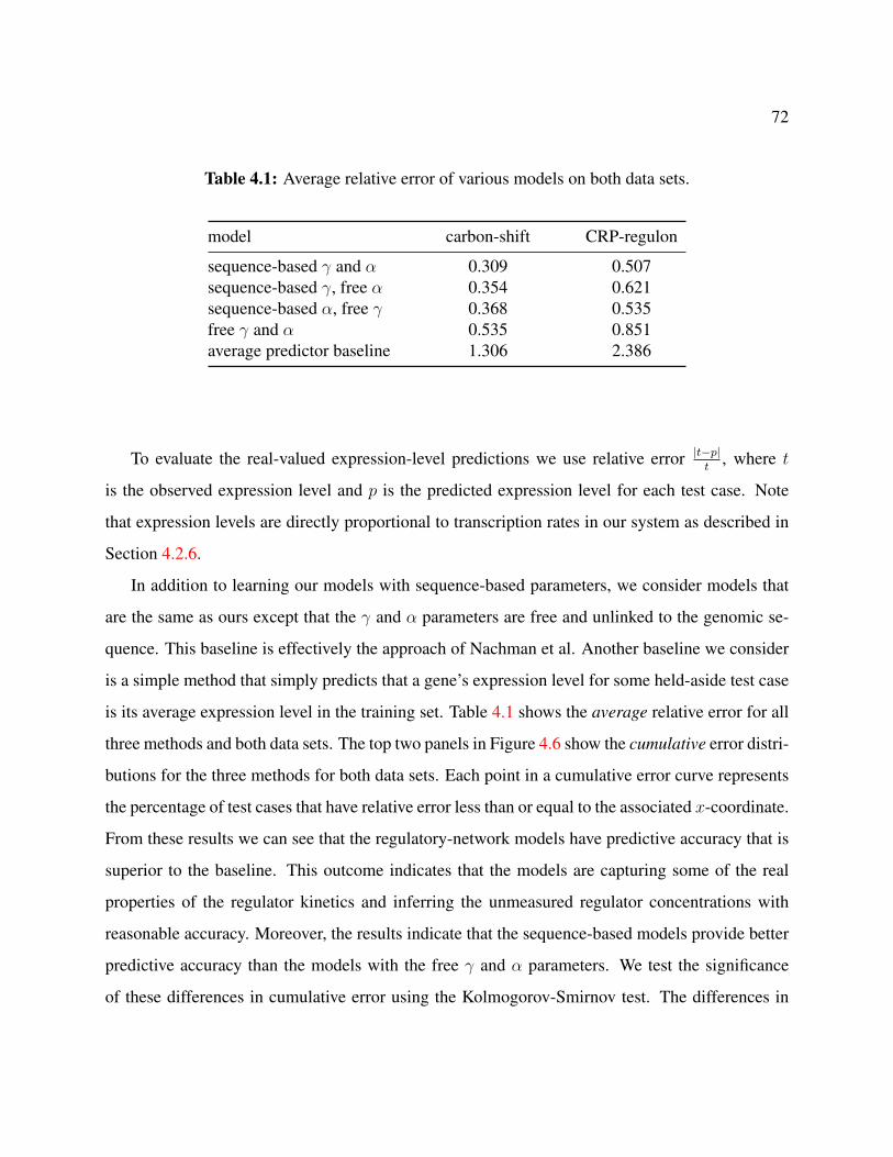
72

Table 4.1: Average relative error of various models on both data sets.

model carbon-shift CRP-regulon

sequence-based γ and α 0.309 0.507sequence-based γ, free α 0.354 0.621sequence-based α, free γ 0.368 0.535free γ and α 0.535 0.851average predictor baseline 1.306 2.386

To evaluate the real-valued expression-level predictions we use relative error |t−p|t

, where t

is the observed expression level and p is the predicted expression level for each test case. Note

that expression levels are directly proportional to transcription rates in our system as described in

Section 4.2.6.

In addition to learning our models with sequence-based parameters, we consider models that

are the same as ours except that the γ and α parameters are free and unlinked to the genomic se-

quence. This baseline is effectively the approach of Nachman et al. Another baseline we consider

is a simple method that simply predicts that a gene’s expression level for some held-aside test case

is its average expression level in the training set. Table 4.1 shows the average relative error for all

three methods and both data sets. The top two panels in Figure 4.6 show the cumulative error distri-

butions for the three methods for both data sets. Each point in a cumulative error curve represents

the percentage of test cases that have relative error less than or equal to the associated x-coordinate.

From these results we can see that the regulatory-network models have predictive accuracy that is

superior to the baseline. This outcome indicates that the models are capturing some of the real

properties of the regulator kinetics and inferring the unmeasured regulator concentrations with

reasonable accuracy. Moreover, the results indicate that the sequence-based models provide better

predictive accuracy than the models with the free γ and α parameters. We test the significance

of these differences in cumulative error using the Kolmogorov-Smirnov test. The differences in

73

0.1 0.3 0.5 0.7 0.9 1.1 1.3 1.5 1.7 1.9 4 8 12 16 20

Cumulative relative error

0

10

20

30

40

50

60

70

80

90

100

Test

case

s(%

)

Carbon Shift Data Set

sequence-based andfree andbaseline: averaging known values

0.1 0.3 0.5 0.7 0.9 1.1 1.3 1.5 1.7 1.9 4 8 12 16 20

Cumulative relative error

0

10

20

30

40

50

60

70

80

90

100

Test

case

s(%

)

CRP Regulon Data Set

sequence-based andfree andbaseline: averaging known values

0.1 0.3 0.5 0.7 0.9 1.1 1.3 1.5 1.7 1.9 4 8 12 16 20

Cumulative relative error

0

10

20

30

40

50

60

70

80

90

100

Test

case

s(%

)

sequence-based andsequence-based , freesequence-based , free

0.1 0.3 0.5 0.7 0.9 1.1 1.3 1.5 1.7 1.9 4 8 12 16 20

Cumulative relative error

0

10

20

30

40

50

60

70

80

90

100

Test

case

s(%

)

sequence-based andsequence-based , freesequence-based , free

Figure 4.6: Cumulative error distributions of various models. Panels on the left and right show10-fold cross validation results on carbon-shift data set and CRP-regulon data set,respectively. The top panels show error distributions for the sequence-based models,free-γ and α models, and baseline. The bottom panels show error distributions for thelesion experiments, with the sequence-based models shown for reference purposes.

74

cumulative error between the sequence-based and free-γ/α models are significant at p = 0.019 for

the carbon-shift data set and p = 0.001 for the CRP-regulon data.

In order to test whether the predictive gain of the sequence-based models is coming from the

sequence-based γ functions alone or the sequence-based α functions alone, we conduct two “le-

sion” tests. Each lesion test involves running our approach with either the sequence-based binding

(γ) or productivity (α) functions replaced with free parameters (i.e., γ parameters are sequence-

based but α parameters are not, and vice versa). Table 4.1 and the bottom two panels in Figure 4.6

show that running our model with both parameter types represented as sequence-based functions

results in more accurate predictions than with only one parameter type represented in this way.

4.3.3 Evaluating Model Explanatory Power

In addition to making accurate predictions (which a “black-box” model may do well) we also

wish to gain insight into the underlying regulation properties represented by our learned models.

We argue that models with more explanatory power can better help biologists understand observed

regulation phenomena and potentially aid in predicting the outcomes of biological manipulations,

such as promoter-sequence mutations.

Toward this end, we first evaluate the learned RNAP concentration profile from the carbon-shift

data set, for which we have some prior biological knowledge. Figure 4.7 shows the relative con-

centration inferred from the model with sequence-based γ and α parameters, and from the model

with free γ and α parameters. Although both models infer somewhat similar RNAP profiles for

glycerol, succinate and alanine relative to glucose, they are dramatically different for the relative

levels of acetate and proline. Previous studies [Ishihama, 1981; Ishihama et al., 1976] show that the

available RNAP levels are highly similar in growth culture with acetate and proline as the carbon

source. The almost 10-fold concentration increase inferred by the model with free γ and α pa-

rameters therefore is not in agreement with current knowledge. The RNAP concentration profiles

inferred by our sequence-based models are more accurate in this respect.

We also assess the biological significance of the weights learned from our RNAP productivity

model. Since we do not have ground truth to directly consult, we compare our learned weights

75

glucose glycerol succinate alanine acetate proline

Carbon source

0.0

0.2

0.4

0.6

0.8

1.0A

vaila

ble

RN

AP

conc

entr

atio

n

sequence-based andfree and

Figure 4.7: Inferred available RNAP concentrations in carbon shift experiments. Values arescaled such that maximum concentration is one unit.

to the weights learned by a regression model trained on a whole-genome in vitro transcription

data set produced by the Burgess lab at University of Wisconsin-Madison. In these assays, RNA

products from transcription reactions using MG1655 genomic DNA and purified E. coli RNAP

were hybridized to Affymetrix E. coli GeneChips. The resulting signal intensity for any given

operon is a reflection of the intrinsic strength of the corresponding promoter as no transcription

factors were present to influence RNAP-promoter interactions. The experiment was done in two

biological replicates. Normalized signal intensity values for each gene were averaged and genes

with intensities greater than 9 (log2 scale) were chosen for further analysis. This cutoff was used

to ensure that the selected genes were unambiguously transcribed in the experiment. Next, to

limit subsequent analysis to only those genes with experimentally defined promoter sequences, the

gene subset was compared against data culled from the EcoCyc database [Keseler et al., 2005] to

76

identify those with known transcription start sites. In cases where an operon contains more than

one gene, only the first gene in that operon was chosen for the analysis. This procedure resulted in

82 promoter sequences.

From this data set we induce various regression models, using the WEKA library [Witten and

Frank, 2005], that map the promoter sequences to their associated in vitro expression levels. We

represent the promoter sequences using features extracted by the HMM described in Section 4.2.4.

The features used to represent these promoters are the same as the ones used in the RNAP pro-

ductivity model. Among the best regression models induced in this study is one based on a linear

regression method that minimizes mean squared error. Figure 4.8 shows a scatter plot of expres-

sion values predicted by this model versus the measured expression values. Although the accuracy

of the model is not exceptional, it does have some predictive power. The correlation coefficient

between the predicted and measured values is 0.65.

We compare the weights from this in vitro model against the weights learned in the RNAP

α model when it is trained on the carbon-shift data set. The key distinction between these two

models is that whereas the former is given a direct training signal (in vitro expression levels),

the latter must infer its weights in the context of a more sophisticated model that is (i) taking

into account the role of transcription factors, (ii) inferring activity levels of these regulators, and

(iii) modeling expression in a range of in vivo conditions. Gene expression levels in E. coli are

determined primarily by the rate of transcription initiation which involves multiple kinetic steps,

including RNAP binding, open complex formation and promoter clearance. Weights learned from

the in vitro data should in principle capture the composite impact of a base at a position on the

whole process. Weights in the RNAP α function in our network model, on the other hand, are

expected to represent the same composite effect minus the effect on binding, which is modeled

by the γ parameter. By comparing the RNAP α model to the in vitro model, we believe that we

can garner some evidence indicating whether or not our RNAP α model is learning meaningful

weights.

The most contributing base (the one with highest weight) at each position is shown for both

models in Figure 4.9. We observe the high similarity of the most contributing bases in -35 region

77

......

....

.

.

.

....

.

.......

.

.

.........

.........

.

.

.

.

.

.

.

.

..

..

...

..

.

.

.

.

...

..

.

.

..

.

...

..

.

Figure 4.8: Agreement between predicted and measured expression values on in vitro transcrip-tion profiling data set. The predicted values are from a linear regression model.

(5 out of 6) and some level of similarity in -10 region (2 out of 6). These results demonstrate that

the weights inferred for the RNAP α function in our network model have a reasonably high corre-

spondence to the in vitro weights, and therefore are likely to have some biological significance.

Figure 4.9 also shows the standard consensus sequence for σ70 promoters. Interestingly, neither

our RNAP α model nor the in vitro model learns weights in correspondence with the consensus.

Furthermore, we have evaluated “similarity with the consensus” as an approach to predicting the

in vitro expression values and found that it does not predict nearly as well as the linear regression

model considered here. One possible explanation for these results is that the consensus sequence

78

Figure 4.9: The most contributing base at each position of the E. coli promoter -35 and -10 regionsvs. promoter consensus. The row labeled In vitro model represents the bases withthe largest weights at each position in the linear regression model trained on the invitro transcription data. The row labeled Network alpha model represents the baseswith the largest weights at each position in the RNAP productivity function, whichis learned in the regulatory-network model. The row labeled Consensus shows thestandard E. coli σ70 consensus sequence.

characterizes the sequence properties that are more important for sequence binding than for the

other steps involved in transcription initiation.

4.4 Summary

We have presented our extension to a state-of-the-art approach for inferring quantitative gene-

regulatory network models. Our method represents and learns the key kinetic parameters of tran-

scription regulation as functions of features in the genomic sequence. The primary motivation

for our approach is to offer more explanatory power than models without these sequence-based

functions. Our experiments on two E. coli expression data sets indicate several key results. First,

models with sequence-based kinetic parameters are more accurate than models without. Second,

the models learned with sequence-based kinetic parameters produced more biologically-sound ac-

tivity profiles for active RNAP. Third, the sequence-based α function learned for RNAP captured

some aspects of the binding site that are in agreement with a model trained directly on controlled

in vitro data.

79

Chapter 5

Discovering Hidden Regulators of Gene Regulatory Networks

5.1 Introduction

In Chapter 4, I elaborate my approach to learning the values of kinetic parameters and activity

levels of regulators. The learning task there assumes a predefined and fixed regulatory-network

structure (i.e., which regulators regulate each gene), and aims to infer accurate and biologically

relevant numerical values of kinetic parameters and regulator activities. Such a predefined net-

work structure could come from background knowledge such as the biological literature. How-

ever, background knowledge regarding the relevant regulators in an organism or in a particular

cellular process is often incomplete. This means some genes in regulatory network models may be

missing important regulators when the regulators in these network models are determined based

on background knowledge. Such a predefined network structure could also come from the output

of an independent learning procedure that determines which regulators control each gene for a

collection of its input genes and regulators, without any prior knowledge of regulator-gene rela-

tionships. However, we may not have, as input for this procedure, all the relevant regulators for

the genes of interest. Therefore the output of this independent learning procedure will not give us

the complete network structure either, because there are missing regulators in its input. In short,

a network-model structure may have missing regulators when such a model structure is either

built from background knowledge or determined by another independent procedure that learns the

network-model structure ab initio.

So why do we have missing regulators for genes of interest in the first place? Let us consider

the following two scenarios. In Scenario 1, a missing regulator might be one whose identity is

80

not known at all in an organism, i.e., it is a novel regulator not previously discovered yet, such

as an unreported transcription factor. In Scenario 2, a missing regulator may correspond to one

whose identity is known in an organism, but whose role in the cellular process being studied is not

recognized. That is, prior knowledge does not indicate that this regulator is relevant to the process

being studied. For example, we may know that a particular transcription factor exists in E. coli

(and even know it is involved in an E. coli heat-shock response, etc.), but we do not know that it

also participates in an E. coli oxygen-shift response we study. Therefore, this transcription factor is

a missing regulator for certain genes involved in this oxygen-shift response. I refer to the missing

regulators in the above two scenarios as hidden regulators from now on.

Note that a regulator here could be a protein (e.g., transcription factor), a RNA (e.g., antisense

RNA), a protein-protein complex, or a protein-metabolite complex, among others. In the work

here we simply assume the regulator has binding sites in regulatory regions of its target genes.

Also note that hidden regulators can be represented by hidden variables in models like Bayesian

networks, but the meaning of “hidden” is different. “Hidden” in hidden regulators emphasizes

that the regulators and corresponding variables themselves are missing; while “hidden” in hidden

variables means those variables are present in models but their values/states are unmeasured or

unknown—hidden variables can represent hidden regulators, known regulators, or other entities.

The goal of regulator discovery in this chapter is to use computational tools to find, for given

cellular processes, which genes may have hidden regulators and the binding sites of these hidden

regulators in regulatory regions of target genes. The focus here is on which genes are regulated by

each of these hidden regulators, not the identities of these hidden regulators themselves. That is, the

discovered/proposed hidden regulators may be anonymous. The identity of a hidden regulator can

be further examined by experimental biologists using biochemical techniques, or by computational

biologists using database searching tools.

In this chapter, I describe an approach to discovering these hidden regulators and their binding

sites in target genes using gene expression and genomic sequence data. The rest of this chapter is

organized as follows. Section 5.2 describes the primary motivation for my computational approach

to discovering hidden regulators. Section 5.3 compares and contrasts my approach with previous

81

computational methods, and discusses how my new framework extends the previous state of the

art. Section 5.4 describes the technical details of my algorithm. Section 5.5 presents experiments to

evaluate my approach to regulator discovery using E. coli as a model organism. Section 5.6 shows

a case study of hidden regulator discovery. Finally, Section 5.7 offers a summary of contributions.

5.2 Motivation

The task of hidden regulator discovery is important in that the discovered hidden regulators

could be critical for the cellular processes being studied; therefore such knowledge discovery can

potentially advance our understanding of gene regulation of cellular phenomena that are essential

to an organism’s survival, adaptation and evolution, etc.

Traditionally, biologists have discovered regulators through biochemical, molecular or physio-

logical methods that usually require large-scale human efforts. The scale of such biological study

is usually small since such experiments are typically conducted at a particular pathway level; the

time and cost involved are fairly high due to the nature of many bench experiments. Over the last

decade, the high-throughput technique ChIP-chip [Aparicio et al., 2004] has been developed to

investigate interactions between proteins and DNA in vivo. Although the ChIP-chip technique en-

ables the identification of binding sites of DNA-binding proteins on a genome scale, it is expensive

and requires highly specific antibodies that recognize proteins of interest. Furthermore, ChIP-chip

technique will not help when the identities of hidden regulatory proteins are unknown ahead of

time (therefore we do not know the corresponding antibodies), or when the hidden regulators are

not protein molecules.

Compared to the above experimental approaches, the work in this chapter is focused on devel-

oping computational tools to automatically propose/discover hidden regulators based on available

biological data, without human intervention. The approach I present is capable of handling the

task of regulator discovery at the genome scale. That is, models in my computational approach can

include all the genes in an organism like E. coli. More importantly, the identities of hidden regula-

tors are not assumed to be known in my computational approach; and these hidden regulators are

not assumed to be proteins—they could be other DNA-binding factors.

82

However, the primary motivation of this work is not to largely replace human bench experi-

ments. Instead, the primary motivation is to suggest potential hidden regulators with biologically

interpretable evidence to assist biologists in discovering hidden regulators and their binding sites

in the regulatory regions of target genes. Ultimately, these suggested hidden regulators need to

be experimentally tested and verified by experimental biologists. In other words, my approach

would hopefully reduce the search effort and experimental cost when biologists attempt to identify

promising hidden regulators and their target genes.

5.3 Previous Methods vs. My Method

Previous computational approaches to discovering hidden regulators can be roughly divided

into two groups: expression clustering-based and expression modeling-based approaches.

Expression clustering-based approaches first identify groups of genes with similar expression

patterns over a set of experiments or a series of time points. The genes in each group are assumed

to have similar regulatory mechanisms, therefore sharing some hidden regulators. A sequence-

motif finding procedure is then applied to the regulatory regions of the genes in each cluster in

order to find binding sites of the putative hidden regulators. An example of expression clustering-

based approaches is presented in Zhang [1999]. Figure 5.1 illustrates this approach. The approach

is procedurally straightforward as it does not need to construct complicated statistical models to

explain the expression data. However, the approach has following disadvantages:

• It cannot take advantage of prior knowledge of the regulators in the experiments or cellular

processes being studied. It does not consider existing regulators at all when searching for

hidden regulators.

• Genes sharing common regulators may or may not have similar expression profiles due to

combinatorial regulation from multiple regulators [Li et al., 2007] (see Section 5.4.3 for

details). Therefore, this approach would sometimes assign genes sharing a hidden regulator

into distinct clusters.

83

Motif-finding for individual clusters

Figure 5.1: Illustration of the expression clustering-based approach to regulator discovery. Thecolored image represents clustered expression levels of certain genes in various con-ditions. Each gene is represented by a single column of colored boxes; each exper-imental condition is represented by a single row. Gene names are above and belowthe colored image. The dendrogram (tree structure shape) on the top represents thecorresponding hierarchical clustering tree with distance-measure scale on its left side.In this example, the approach first clusters gene expression profiles across conditionsusing a hierarchical clustering method, then identifies two clusters of genes with sim-ilar expression patterns (indicated by black bars): one cluster has four genes and theother has six genes. Next, for each cluster, the regulatory regions of the genes in thatcluster are examined by a motif-finding tool in order to search for putative bindingsites of potential hidden regulators.

84

• Although this approach considers sequence evidence (i.e., DNA motifs) when proposing

hidden regulators, it relies on plug-in motif finders to rank candidate motifs and thus cor-

responding candidate hidden regulators. An employed plug-in motif finder may or may not

determine the most relevant sequence motifs correctly.

Expression modeling-based approaches attempt to infer gene regulatory-network models to ex-

plain the observed gene expression data. For example, Noto and Craven [2005] and Nachman et al.

[2004] encode regulators, genes, and their relationships in Bayesian network models and optimize

certain likelihood functions that take into account the gene expression data and the activity levels

of regulators. Roughly speaking, they model the likelihood of seeing the expression data given a

set of regulator-gene relationships. New regulators are proposed when they can improve the likeli-

hood, i.e., better explain the expression data. The advantages of such modeling-based approaches

include incorporating prior regulator-gene relationships, handling noise in data in principled ways,

and accounting for the processes that generate the expression data.

However, one disadvantage of such approaches is that they consider only one type of high-

throughput data, gene expression measurements, when proposing hidden regulators. Although

these approaches attempt to handle noise, still spurious regulators might be added into network

models to “explain” the noise in the expression data.

Compared to these previous computational approaches to discovering hidden regulators, my

approach incorporates several innovations and integrates them into a new framework as follows:

• First, a biochemical kinetics-based and genome sequence-connected network model utilizes

prior knowledge about regulator-gene relationships to explain observed gene expression pro-

files. This quantitative model takes advantage of knowledge about known regulators, and can

easily accommodate new regulators when the knowledge of regulators is updated.

• Second, weakly explained genes are identified and then clustered based on their error profiles

(to be explained in Section 5.4.3) rather than expression profiles, in order to capture the

effects of hidden regulators. A list of weakly explained genes narrows the search space

down to genes that are more likely to have important hidden regulators.

85

• Third, DNA motifs corresponding to hidden regulators are proposed based on the putative

binding sites in the upstream sequences of genes. Compared to approaches that propose

hidden regulators based on gene expression data alone, my approach considers both gene

expression and genomic sequence data. Hence, it can provide extra evidence (i.e., physi-

cal regulator binding sites) to support why a hidden regulator might regulate certain genes.

Furthermore, hidden regulators proposed by my approach could be proteins, RNAs, or other

biological entities as long as they have binding sites in regulatory sequences.

• Fourth, binding-site motifs of candidate hidden regulators are post-processed by novel motif

filtering and ranking methods. This step is aimed at selecting accurate and relevant motifs

that correspond to the most promising hidden regulators.

5.4 Approach

In this section, I present my approach to discovering hidden regulators as a flow of data input,

model building and hypothesis generation. I also further discuss the innovations in my approach.

This approach does not assume a particular organism, although I empirically evaluate the approach

using data from E. coli K-12.

Formally, the task I address in this chapter is to infer hidden regulators in gene regulatory

networks from biological data, as follows.

Given:

• measurements of gene expression levels,

• regulatory sequences of genes,

• known regulator-gene relationships,

• coding sequences of genes (optional, for cross-species comparison).

Do:

• propose or discover hidden regulators and their binding sites in the regulatory

sequences of target genes,

86

• rank candidate hidden regulators based on their binding-site motifs.

My approach starts with a Bayesian network model that uses background or user-specified

regulator-gene relationships to explain observed gene expression data. If important regulators are

missing in the current network model (i.e., there are hidden regulators), the expression of some

genes will not be explained well by the current model. Those weakly explained genes are singled

out, and then are clustered based on their error profiles. A gene’s error profile describes the dis-

crepancies between that gene’s actual transcription rates and model-predicted transcription rates,

therefore reflecting the effects of putative hidden regulators. We hypothesize that genes with sim-

ilar error profiles are likely to share the same hidden regulators in the cellular processes being

modeled. Next, a motif finder is employed to search the regulatory sequences of genes in each

cluster, and the resulting motifs from each cluster are pooled. Finally, novel motif filtering and

ranking methods are developed to post-process the pooled motifs, in hope of removing spurious

ones and identifying the most promising ones. Hidden regulators are proposed based on the re-

maining ranked motifs. Whether these proposed hidden regulators are activators or repressors can

be further examined; and then the discovered hidden regulators can be added into the current model

to refine the model structure. Figure 5.2 illustrates the flow of this approach. I now describe the

steps of this approach in detail.

5.4.1 Initializing the Network Structure

To initialize the network structure, i.e., to connect regulators to their target genes in a network

model, one can acquire regulatory information of a species from the biological literature or online

databases. In the case of E. coli, such known TF-gene regulatory relationships can be downloaded

from RegulonDB [Gama-Castro et al., 2008] or EcoCyc [Keseler et al., 2009]. Since regulators

influence gene expression in specific cellular conditions, we can optionally filter out those known

regulators that are believed not to function in the set of experiments being studied.

When such background knowledge is not available, the network structure can be initialized

based on user-specified regulator-gene relationships. These user-specified regulatory relationships

87

Gene

Max

Err

or

Network Model

Error for experiment 1

Erro

r for

exp

erim

ent 2

Gene

Max

Err

or

a b c

Mot

if R

ank

f e d

Threshold

GeneClustering

Figure 5.2: Flow of the hidden regulator discovery approach. The inputs for this pipeline aregene expression and genomic sequence data. In particular, gene mRNA levels acrossexperiments (or time series), upstream regulatory sequences of genes, and binding-site sequences of known regulators in their target genes (these inputs are not shown inthe figure). Caption continues on next page.

88

Figure 5.2: (See previous page. Caption continues from previous page.)

(a) The parameters are learned in a biochemically based quantitative regulatory-network model. In this model, pink nodes denote regulators and their unmeasured ac-tivity levels; brown nodes denote genes and their recovered transcription rates whichare derived from their mRNA levels. A green edge indicates a gene is activated by aregulator; while a red edge indicates a gene is repressed by a regulator. The initialnetwork structure is derived from background knowledge.

(b) Given learned parameters, we compute a relative error between each gene’s re-covered transcription rate and the gene’s predicted transcription rate for each exper-iment. Subsequently, we know the maximal relative error (denoted as Max Error inthe panel) of each gene across experiments. In this example, eight genes and theirmaximal relative errors are plotted.

(c) Given a threshold on the maximal relative error, we identify a subset of geneswhose errors are larger than this threshold. These genes are weakly explained genes(see Section 5.4.2). Five out of eight genes are weakly explained in this example.

(d) The weakly explained genes are then clustered based on their error profiles, i.e.,their relative errors across experiments. In this example, five weakly explained genesform two clusters based on their error profiles across two experiments.

(e) For each cluster of genes, a motif finder is applied to search for DNA motifs in theregulatory sequences of genes in the cluster. The motifs suggested by the motif finderfor each cluster are pooled. In this example, a total of six motifs are pooled from theprevious two clusters.

(f) The pooled motifs are post-processed by motif filtering and ranking methods, inhope of removing spurious motifs as well as identifying the most promising motifs(see Section 5.4.5). Each non-redundant motif corresponds to a putative hidden regu-lator.

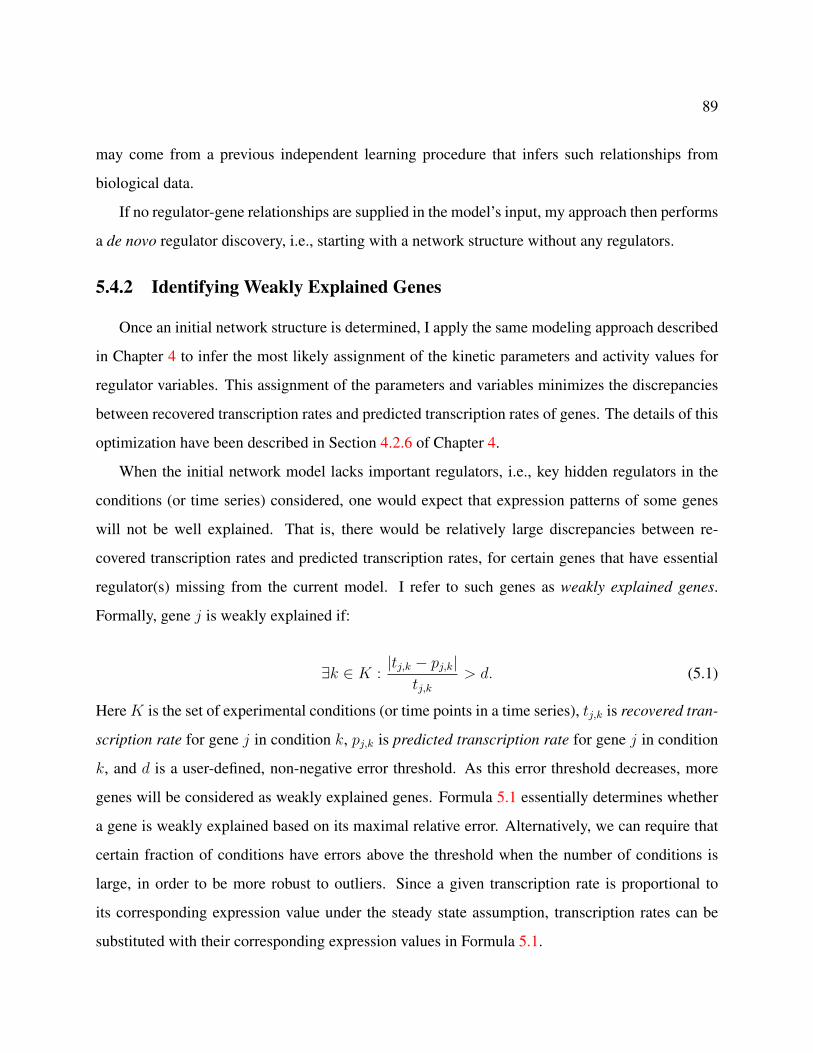
89

may come from a previous independent learning procedure that infers such relationships from

biological data.

If no regulator-gene relationships are supplied in the model’s input, my approach then performs

a de novo regulator discovery, i.e., starting with a network structure without any regulators.

5.4.2 Identifying Weakly Explained Genes

Once an initial network structure is determined, I apply the same modeling approach described

in Chapter 4 to infer the most likely assignment of the kinetic parameters and activity values for

regulator variables. This assignment of the parameters and variables minimizes the discrepancies

between recovered transcription rates and predicted transcription rates of genes. The details of this

optimization have been described in Section 4.2.6 of Chapter 4.

When the initial network model lacks important regulators, i.e., key hidden regulators in the

conditions (or time series) considered, one would expect that expression patterns of some genes

will not be well explained. That is, there would be relatively large discrepancies between re-

covered transcription rates and predicted transcription rates, for certain genes that have essential

regulator(s) missing from the current model. I refer to such genes as weakly explained genes.

Formally, gene j is weakly explained if:

∃k ∈ K :|tj,k − pj,k|

tj,k> d. (5.1)

Here K is the set of experimental conditions (or time points in a time series), tj,k is recovered tran-

scription rate for gene j in condition k, pj,k is predicted transcription rate for gene j in condition

k, and d is a user-defined, non-negative error threshold. As this error threshold decreases, more

genes will be considered as weakly explained genes. Formula 5.1 essentially determines whether

a gene is weakly explained based on its maximal relative error. Alternatively, we can require that

certain fraction of conditions have errors above the threshold when the number of conditions is

large, in order to be more robust to outliers. Since a given transcription rate is proportional to

its corresponding expression value under the steady state assumption, transcription rates can be

substituted with their corresponding expression values in Formula 5.1.

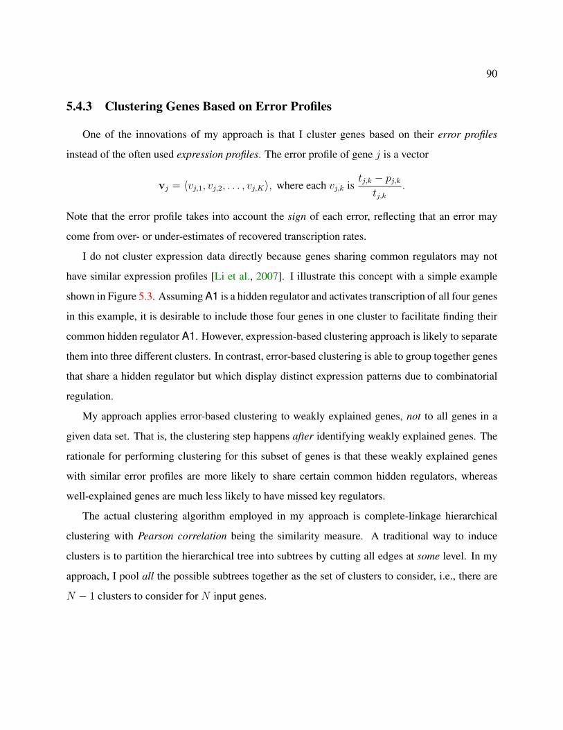
90

5.4.3 Clustering Genes Based on Error Profiles

One of the innovations of my approach is that I cluster genes based on their error profiles

instead of the often used expression profiles. The error profile of gene j is a vector

vj = 〈vj,1, vj,2, . . . , vj,K〉, where each vj,k istj,k − pj,k

tj,k.

Note that the error profile takes into account the sign of each error, reflecting that an error may

come from over- or under-estimates of recovered transcription rates.

I do not cluster expression data directly because genes sharing common regulators may not

have similar expression profiles [Li et al., 2007]. I illustrate this concept with a simple example

shown in Figure 5.3. Assuming A1 is a hidden regulator and activates transcription of all four genes

in this example, it is desirable to include those four genes in one cluster to facilitate finding their

common hidden regulator A1. However, expression-based clustering approach is likely to separate

them into three different clusters. In contrast, error-based clustering is able to group together genes

that share a hidden regulator but which display distinct expression patterns due to combinatorial

regulation.

My approach applies error-based clustering to weakly explained genes, not to all genes in a

given data set. That is, the clustering step happens after identifying weakly explained genes. The

rationale for performing clustering for this subset of genes is that these weakly explained genes

with similar error profiles are more likely to share certain common hidden regulators, whereas

well-explained genes are much less likely to have missed key regulators.

The actual clustering algorithm employed in my approach is complete-linkage hierarchical

clustering with Pearson correlation being the similarity measure. A traditional way to induce

clusters is to partition the hierarchical tree into subtrees by cutting all edges at some level. In my

approach, I pool all the possible subtrees together as the set of clusters to consider, i.e., there are

N − 1 clusters to consider for N input genes.

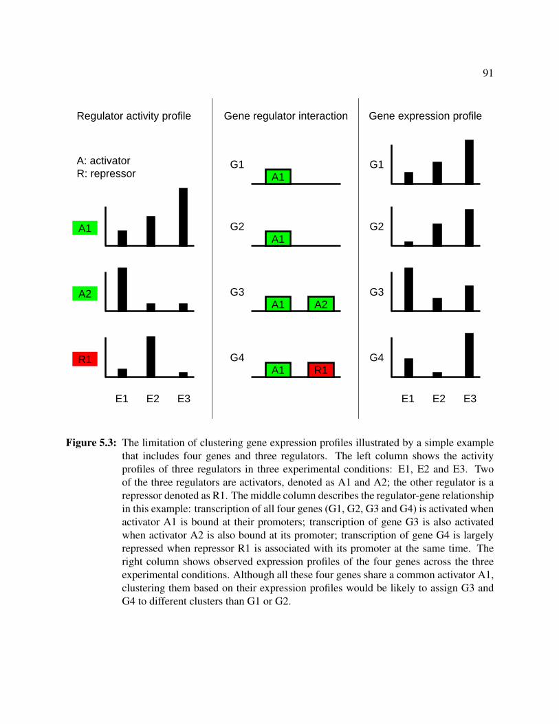
91

1

G1 G1A1

A1

A1 A2

A1 R1

A1

A2

R1

E1 E2 E3 E1 E2 E3

Regulator activity profile Gene regulator interaction Gene expression profile

G2 G2

G3 G3

G4 G4

A: activatorR: repressor

Figure 5.3: The limitation of clustering gene expression profiles illustrated by a simple examplethat includes four genes and three regulators. The left column shows the activityprofiles of three regulators in three experimental conditions: E1, E2 and E3. Twoof the three regulators are activators, denoted as A1 and A2; the other regulator is arepressor denoted as R1. The middle column describes the regulator-gene relationshipin this example: transcription of all four genes (G1, G2, G3 and G4) is activated whenactivator A1 is bound at their promoters; transcription of gene G3 is also activatedwhen activator A2 is also bound at its promoter; transcription of gene G4 is largelyrepressed when repressor R1 is associated with its promoter at the same time. Theright column shows observed expression profiles of the four genes across the threeexperimental conditions. Although all these four genes share a common activator A1,clustering them based on their expression profiles would be likely to assign G3 andG4 to different clusters than G1 or G2.

92

5.4.4 Motif Finding for Clustered Genes

For each of the clusters generated from error profiles, I use existing motif-finding tools to

search for DNA motifs in the regulatory sequences of the genes in a given cluster. Such a motif

can be used as the evidence that some or all the genes in that cluster have “signals” (binding sites)

that might be recognized by a hidden regulator (e.g., a transcription factor) not represented in the

current network model.

Although any motif-finding tool can be applied in this step, I choose MEME [Bailey and Elkan,

1994] and PhyloCon [Wang and Stormo, 2003] for my experiments. MEME is one of the most

widely used tools for searching for novel “signals” in sets of biological sequences. PhyloCon is one

of the motif finders that utilize cross-species comparison to improve the ability to identify motifs.

Unlike many other motif finders that rely on a user-specified motif-length as an input parameter,

these two tools can automatically determine the best length for a putative motif, which makes them

suitable for the task of regulator discovery because the length of a motif (corresponding to a hidden

regulator) is not known a priori. Besides this advantage, MEME was shown to be the best motif

finder for discovering E. coli motifs among the five motif finders evaluated by Hu et al. [2005]; and

it is relatively unsensitive to the choice of parameters [Hu et al., 2005; Tompa et al., 2005], such

as the order of the background Markov models. PhyloCon outperformed four other motif finders

in terms of the accuracy of motif finding on both synthetic and biological sequences, including

intergenic sequences from the E. coli genome [Wang and Stormo, 2003]. PhyloCon considers both

similarities in a given set of sequences and conservation among orthologous sequences. Integrating

these two different axes of information in motif finding has been proven useful by Siddharthan et al.

[2005] and Sinha et al. [2004], among others.

Note that both MEME and PhyloCon are able to search for motifs for some subset of input

DNA sequences. This is important since it is possible that only a subset of sequences in a cluster

contain a shared motif(s).

93

5.4.5 Filtering and Ranking Candidate Motifs

Motif finding remains a complex challenging task despite considerable effort to date [Tompa

et al., 2005]. Finding motifs is difficult because they could be relatively short signals in a set of

much longer sequences, and there is sequence variability among the binding sites of regulators

such as transcription factors.

Typically, a motif finder examines the input set of sequences and uses statistical criteria to score

and rank putative motifs. The top few motifs in the ranked list are suggested as the most likely

motifs. However, spurious motifs might score high by chance, and the binding sites with highest

statistical significance are not necessarily the best predictions of the true motifs [Liu et al., 2002].

Furthermore, when pooling motifs suggested by different motif finders with different scoring met-

rics, or motifs suggested by the same motif finder but from different data sets, it could be beneficial

to have wrapper methods for post-processing these motifs.

One of the novel contributions of my approach is the development of post-processing proce-

dures (i.e., wrapper methods) that have (a) the ability to identify likely spurious motifs and filter

them given the outputs of standalone motif finders, and (b) the power to rank motifs from stan-

dalone motif finders, such that the most promising or relevant ones are pushed to the top of a list

of candidate motifs.

Section 3.4 in Chapter 3 reviews some previous wrapper methods for motif filtering and rank-

ing, and compares and contrasts them with those developed in my approach. It also describes the

motivation of my wrapper methods in detail. In this section, I focus on describing the technical

details of my motif filtering and ranking methods as follows.

5.4.5.1 Filtering Methods

The purpose of filtering methods is to remove likely spurious motifs from a set of candidate

motifs. The first filtering method I consider simply checks the sequence length (in nucleotide, nt

for short) of a motif to see if the length falls in some reasonable range. Such range can be learned

from some training examples. For example, the motifs of known transcription factors in E. coli can

tell us the min and max length of known E. coli motifs. If one believes that this range of lengths

94

0

1

2

3

4

5

6

7

8

9

10

11

12

13

0 5 10 15 20 25 30 35 40 45 50 55 60

Cou

nt

Motif Length (nt)

Figure 5.4: A histogram illustrating the motif length distribution of known E. coli transcriptionfactors from RegulonDB excluding the nine transcription factors in the model evalu-ated in Section 5.5.

covers most of the actual motifs in E. coli, then it can be used to filter putative E. coli motifs with

lengths outside this range. In other words, we can build species-dependent, length-based motif

filters to remove likely spurious motifs.

Figure 5.4 shows the motif length distribution of known E. coli transcription factors from the

RegulonDB database. Nine motifs, corresponding to the nine transcription factors in the model

evaluated in Section 5.5, are excluded from this distribution. This is because the motifs to be

tested (in this case the nine motifs) should not be used as “training examples” to construct the

motif length distribution. Figure 5.4 indicates that the number of long (> 40 nt) or short (< 10 nt)

motifs is small in E. coli. This figure also indicates the most common motif length is 19 nt long

among the known E. coli motifs from RegulonDB, and 12 known motifs are of this length.

95

The second filtering method I consider involves removing motifs whose nucleotide information

content does not appear to be like those of known motifs. Given a DNA motif induced from the

alignment of n binding sites of the corresponding regulator (such as the motif shown in Figure 2.7

in Chapter 2), the information content of position i in this DNA motif (as described in [Schneider

and Stephens, 1990]) is given by:

Ri = 2− (Hi + en),

where Hi is the entropy of position i and is calculated as:

Hi = −∑a

(fa,i × log2fa,i).

Here, a ∈ {A,C,G, T}, fa,i is the frequency of nucleotide a at position i, and en is a small-sample

correction for the alignment of n binding sites. For nucleotides, the small-sample correction, en,

is given by:

en =1.5

ln2× n.

Thus, the information content of nucleotide a at position i is given by:

Ba,i = Ri × fa,i.

We can sum the information content of nucleotide a across all positions in this DNA motif, nor-

malized by the total information content of the motif, to derive the fraction of information content

of nucleotide a in this motif. Formally, the fraction of information content of nucleotide a in a

motif of length L, Fa, is given by:

Fa =

∑Li=1Ba,i∑Li=1Ri

.

Thus, for a given motif induced from a collection of regulator binding sites, I calculate the

fraction of information content for each of the four nucleotides (i.e., A, C, G, T) in that motif.

Furthermore, I perform such calculation for each of the motifs in a library of known motifs in a

species. Then, for each nucleotide, a “range” can be determined to cover that nucleotide’s fractions

of information content across known motifs. Once we have such a range for each of the four

96

0

5

10

15

20

25

30

35

0.1 0.2 0.3 0.4 0.5 0.6 0.7 0.8 0.9 1

Cou

nt

Fraction of Information Content

A

0

5

10

15

20

25

30

35

0.1 0.2 0.3 0.4 0.5 0.6 0.7 0.8 0.9 1

Cou

nt

Fraction of Information Content

C

0

5

10

15

20

25

30

35

0.1 0.2 0.3 0.4 0.5 0.6 0.7 0.8 0.9 1

Cou

nt

Fraction of Information Content

G

0

5

10

15

20

25

30

35

0.1 0.2 0.3 0.4 0.5 0.6 0.7 0.8 0.9 1

Cou

nt

Fraction of Information Content

T

Figure 5.5: Histograms illustrating the distribution of the fraction of information content of thefour nucleotides in known E. coli motifs from RegulonDB excluding the nine tran-scription factors in the model evaluated in Section 5.5.

nucleotides, we can filter out a putative motif if the fraction of information content of any of its

four nucleotides does not fall in the corresponding range.

Figure 5.5 illustrates, for each of the four nucleotides, the distribution of its fraction of in-

formation content across known E. coli motifs from RegulonDB. Again, the aforementioned nine

motifs are excluded when constructing the four histograms in this figure for the same reason men-

tioned before. For each of the four nucleotides, its fractions of information content, calculated

from known motifs, are assigned into 10 bins with an equal interval. That is, the range of the

first bin is [0, 0.1), and the range of the second bin is [0.1, 0.2), and so on. Figure 5.5 shows that

nucleotides A (red) and T (purple) are more common in E. coli motifs than nucleotides C (green)

and G (blue).

97

5.4.5.2 Ranking Methods

The purpose of ranking methods is to order a set of putative motifs in the hope that the correct

or most relevant motifs rank at the top of a list, while false or spurious motifs fall at the bottom.

I design two ranking methods in my approach. The first one is based on using a permutation

test to assess the statistical significance of motifs. Given a motif proposed by some motif finder,

labeled with a score quantifying the importance of this motif (e.g., log likelihood ratio), I compute

the probability of seeing a score equal to or better than the observed score when the same number

of randomly selected regulatory sequences from the same species is used as the input for the same

motif finder. Motifs are then ranked by these probabilities. In this permutation test, the null

distribution of the motif scores is obtained by calculating all possible values of the motif score

when randomly choosing the same number of sequences from the genome of the same species. I

refer to this ranking method as rank-by-significance.

Note that many motif finders have “built-in” scoring methods for determining the statistical

significance of putative motifs. However, they often assume particular score distributions. In

contrast, my rank-by-significance method is based on the concept of a non-parametric distribution

(i.e., a specific distribution is not assumed for the motif scores), and thus is easy to understand and

general enough to be applicable to many existing motif finders. The probability calculated by

rank-by-significance corresponds to the widely used p-value, making a threshold choice fairly

comprehensible. Moreover, when ranking the motifs suggested by different motif finders, the

built-in scoring metrics might be different across motif finders. Therefore, scores might not be

comparable across different motif finders. In contrast, rank-by-significance can post-process

motif scores from different motif finders, and make them comparable.

The second ranking method not only takes into account the characteristic of the motifs them-

selves, but also considers how the presence of a motif in regulatory sequences of genes relates

to the prediction errors that are made on those genes by a network model. Given a motif can be

represented as a position weight matrix (described in Chapter 2) which is built on the basis of the

set of estimated binding sites, I use such a position weight matrix to scan the regulatory sequences

(e.g., promoters) of genes in the model. For a given gene, I find the most likely place such a

98

motif might reside in that gene’s regulatory region. This likelihood is calculated as a log-ratio

of two probabilities for a piece of regulatory sequence segment S with the same length L as the

motif: The probability of observing S given the motif model (the matrix), and the probability of

observing S given the background model (the genomic context). After scoring all the possible

sequence segments of length L in the regulatory sequence of gene j, the highest likelihood score,

denoted as scorej is saved for gene j. Recall that each gene also has an error profile described

in Section 5.4.3. I denote the largest absolute value in the error profile (i.e., vector) of gene j as

errorj . Thus, for each motif, I compute the Pearson correlation coefficient between the following

two vectors:

score = 〈score1, score2, . . . , scoreJ〉

error = 〈error1, error2, . . . , errorJ〉

where J corresponds to the total number of genes in the network model, not just the weakly ex-

plained genes. Note that, the error vectors are the same in the calculation for each motif, but

the score vectors vary for different motifs. Subsequently, candidate motifs can be ranked by their

Pearson correlation coefficients. I refer to this ranking method as rank-by-correlation.

The primary motivation for designing this rank-by-correlation is that binding sites of a hid-

den regulator are likely to be more enriched in the regulatory sequences of genes that have high

prediction errors.

5.4.5.3 Combining Both Methods

The individual filtering and ranking methods in my approach can be combined in the following

way to post-process a set of putative motifs: First, redundant motifs (binding sites offset to each

other by one or two nucleotides) are removed to avoid considering essentially the same motifs;

second, both filtering methods are applied to remove those motifs that are unlikely to be actual

binding sites; third, one of the ranking methods is applied to rank the remaining motifs.

Note that, after filtering, the list of motifs might be empty, indicating none of the motifs that

are in the output of a motif finder represents a plausible biological motif. The ranking provides

99

biologists with confidence with respect to the likelihood of finding a true motif as well as a “knob”

for controlling sensitivity and specificity of regulator discovery.

5.4.6 Proposing Hidden Regulators

Based on the above ranked list of candidate motifs, we can propose putative hidden regulators

and their corresponding target genes. In particular, biologists can decide how far they want to go

down the ranked motif list to select top motifs (and thus their corresponding hidden regulators). For

each of the selected and ranked motifs, the estimated occurrences of that motif (i.e., the predicted

binding sites of the corresponding regulator) in certain genes indicate that these genes might share

the same hidden regulator.

As stated in Section 5.1, the goal of regulatory discovery in this chapter is to find, for given

cellular processes, which genes may have hidden regulators and the binding sites of these hidden

regulators. The focus is not the identities of these hidden regulators. However, my approach does

include a step that attempts to identify what these hidden regulators are. In particular, a proposed

motif is checked against known motifs in a species by comparing the estimated binding sites of this

motif with the binding sites of known motifs. If the estimated sites overlap known sites by certain

length, then the proposed motif matches a known motif. Therefore, the corresponding hidden

regulator is identified, and this hidden regulator corresponds to a regulator discussed in Scenario

2 in Section 5.1. That is, this proposed motif is highly likely to correspond to a regulator whose

identity is known but whose role in the cellular processes we study is unknown yet. Of course,

the overlapping length is a user-defined parameter that controls the stringency of the binding-site

comparison.

If the binding sites of a proposed regulator do not overlap any known sites sufficiently, then we

still do not know the identity of this regulator yet. Nevertheless, my approach suggests the binding

sites of this potential hidden regulator, and biologists can use such binding-site information to

help examine if this regulator is a new regulator (such regulators are described in Scenario 1

in Section 5.1). In this case, my approach offers hypotheses that are supported by both gene

expression and genomic sequence data.

100

5.5 Empirical Evaluation

In this section, I present experiments designed to evaluate my approach for hidden regulator

discovery. I hypothesize that the innovations in this approach will lead to hidden regulator discov-

ery with high precision. I evaluate my approach using Escherichia coli K-12 (E. coli for short) as

the model organism.

5.5.1 Experimental Data

Gene-expression data, TF-gene relationship data and genomic sequence data from E. coli are

used in evaluating my approach.

The temporal microarray gene-expression data comes from a time course experiment for the

aerobic to anaerobic switch response in E. coli in steady-state culture conditions. The experiment

was previously published by Ernst et al. [2008] and the original data is available at Gene Expression

Omnibus (GEO accession GSE8323).

The microarray data used by Ernst et al. [2008] has 11 samples in total measuring the gene-

expression response at different time points after the change from aerobic to anaerobic conditions.

There is also a control sample based on completely aerobic conditions before shutting off oxygen.

These samples correspond to 0min, 2min, 5min, 15min, 25min, 35min, 45min, and 55min after

shutting off oxygen. Technical replicates were taken for the 5min, 25min, and 55min time points.

Ernst et al. normalized these microarray data as described in Tong et al. [2004].

Ernst et al. also provide known TF-gene relationship data for the above experiments, i.e.,

information about the key transcription regulators in E. coli in response to the lack of oxygen

in the growth conditions. Specifically, two transcription factors, FNR (fumarate-nitrate reductase

regulator) and ArcA (aerobic respiratory control), are known to be the master regulators of this re-

sponse. FNR is a key regulator of respiration and it controls the transcription of many genes whose

functions facilitate adaptation to growth under O2-limiting conditions [Kang et al., 2005; Partridge

et al., 2006, 2007; Salmon et al., 2003, 2005]. Under microaerobic conditions, ArcA induces ex-

pression of several gene products of the central carbon metabolism, which are sensitive to lower

101

levels of oxygen, and it represses many genes of aerobic respiration [Alexeeva et al., 2003; Com-

pan and Touati, 1994; Shalel-Levanon et al., 2005]. NarL and NarP are two other TFs known to be

involved in the aerobic-anaerobic shift response, and both of them regulate expression of several

operons in response to nitrates and nitrites during anaerobic respiration and fermentation [Con-

stantinidou et al., 2006; Overton et al., 2006; Ravcheev et al., 2007]. Although the roles of the

above TFs have been well characterized in aerobic-anaerobic response, the identities and roles of

some other TFs are less clear, which makes this data set an interesting candidate for evaluating my

regulator discovery approach.

I average the replicates at the 5min, 25min, and 55min time points so that there are eight ex-

pression values for individual genes instead of the original 11 ones. I then convert these expression

values to a log base ten ratio relative to the 0 min time point. I selected only genes without missing

time points and with at least a two fold expression fluctuation at some time point in the anaerobic

condition. When more than one gene from the same operon are present, the gene being transcribed

first is used to represent the operon, based on known and predicted E. coli operons [Bockhorst

et al., 2003a]. Finally, genes with at least one curated transcription factor, supported by “direct

evidence” from EcoCyc 11.5, are kept in the data set, while the rest are filtered out. I refer to this

resulting gene expression data set (a total of 75 genes with expression measurements across eight

time points) as the oxygen-shift data set. The “direct evidence” includes annotations of “Site Mu-

tations”, “Binding of Cellular Extracts”, or “Binding of Purified Proteins”. Hence, only TF-gene

interactions supported by strong evidence are included to initialize the topology of the network

for the oxygen-shift data set. Such direct evidence is also used by Ernst et al. to construct their

models.

Note that my approach to discovering hidden regulators does not require that genes in the

network models have strongly evidence-supported transcription factors or even have any known

TFs at all. It is for the purpose of evaluating my approach that every gene in this oxygen-shift data

set has at least one experimentally-verified transcription factor. Figure 5.6 shows the evidence-

supported interactions between TFs and genes in this oxygen-shift data set.

102

IHFFis TdcRNarLFNR TdcANarP ArcA GlpR

Figure 5.6: Strongly evidence-supported transcription factor-gene regulatory interactions in theoxygen-shift data set. In this two-level network structure, the top layer includes nineTFs that are known to be involved in the aerobic-anaerobic shift response; the bottomlayer shows 75 genes regulated by these nine TFs. Arcs connecting a TF and itstarget genes denote the regulatory relationships: green being activation and red beingrepression.

The sequence data for genes in the oxygen-shift response experiment consists of both non-

coding sequences used for searching for putative TF binding sites, and gene-coding sequences

used for identifying orthologous genes in other species. Both types of sequences are retrieved by

the RSAT tool (http://rsat.ulb.ac.be/rsat).

Non-coding sequences are the upstream DNA sequences relative to the transcription start site

of genes in E. coli. For a gene whose transcription start site is unknown, its start codon site is then

considered as the origin (position 0).

I set a gene’s default upstream sequence length to be of 400bp unless another gene is located

within this range. In such a case, the upstream sequence is truncated to prevent overlap with

the neighboring gene. The motivation for searching upstream sequences for motifs is that most

regulatory elements, e.g., TF binding sites, are located in the non-coding regions in E. coli.

Gene-coding sequences, i.e., DNA sequences from start codon to stop codon, are converted into

protein sequences and then used for searching the bidirectional best hit (BBH) [Overbeek et al.,

1999] of each protein. I select Salmonella typhi Ty2, Yersinia pestis Antiqua, Vibrio cholerae,

and Haemophilus influenzae as the reference species for E. coli. These species have been shown

to be effective in aiding the identification of transcription factor binding sites by cross-species

comparison [McCue et al., 2002].

103

It is well known that the sole criterion of BBH is not sufficient to infer orthology between two

genes. So I add a constraint on the percentage of protein identity (min 30%), and on the protein

alignment length (min 50 amino acids) as described in Janky and van Helden [2007].

5.5.2 Evaluation Methodology

To evaluate the effectiveness of my approach to finding hidden regulators, I perform “lesion”

tests on the oxygen-shift data set using the evidence-supported TF-gene regulatory relationships

described above. A lesion test, in this context, follows these steps: (1) leaving out one of the nine

known regulators when initializing the structure of the network model, (2) employing the algorithm

described in Section 5.4 to propose candidate hidden regulators, and then (3) asking the question:

does a proposed regulator match the TF that is left out when the model structure is initialized or

does it seem to match another E. coli TF that may or may not be one of the nine TFs involved in

the aerobic-anaerobic switch response?

Matching the left-out TF is certainly a direct confirmation that this approach is capable of

discovering “hidden” regulators. Matching a TF that is not the left-out one could also mean a

success. This is because the proposed regulator in such a case may correspond to an E. coli TF that

is actually important in the aerobic-anaerobic switch response, but whose role was not represented

in the initial network. I refer to the comparison against the left-out TF as reference-lesion, and the

comparison against any E. coli TF as reference-any.

Whether a proposed regulator matches a certain TF is determined by whether its predicted

binding sites overlap the known binding sites of that particular TF. I use the same criteria for

calling site-overlap as used by Tompa et al. [2005]. That is, a predicted site overlaps a known site

if they overlap by at least one-quarter the length of the known site.

For a list of putative motifs (corresponding to the proposed regulators), I evaluate the accuracy

by determining the number of true positives and false positives when the list is not sorted, and

computing precision-TP curves when the list is ranked. In particular, filtering methods produce

unordered candidate motifs, while ranking methods provide ordered ones. Of course, combining

both filtering and ranking procedures also provides a ranked motif list.

104

I hypothesize that using prior network structure knowledge and motif filtering and ranking

methods can help identify hidden regulators with high precision. I use lesion tests to evaluate the

value of motif filtering and ranking methods, as well as the effects of motif finders. Since the

transcription factors TdcA and TdcR only regulate one target gene in the oxygen-shift data set,

their lesion test results are not shown in evaluation because motif finders usually assume more

than one input regulatory sequence.

5.5.3 The Value of Filtering Methods

In order to test the value of including filtering methods to process candidate motifs, I compare

four different filters to post-process the motifs produced by motif finder PhyloCon on the set of

clusters generated by hierarchical clustering. These four filters are:

• none which does not filter out any motifs and simply serves as the baseline.

• length which uses a length threshold to filter out likely spurious motifs. In this experiment,

motifs with length shorter than 10 nucleotides (nt) are removed. This cutoff is based on

the length distribution of 77 known E. coli motifs from RegulonDB except the nine TFs in

the oxygen-shift data set to avoid overfitting. Figure 5.4 in Section 5.4.5.1 has shown the

frequency of each known motif length. The 10nt threshold is chosen to include 95% of the

known E. coli motifs.

• complexity which removes motifs whose fractions of information content for the four nu-

cleotides do not appear to be within the corresponding ranges of those for known E. coli

motifs (see Section 5.4.5.1). The distributions of the fraction of information content for each

of the four nucleotides (A, C, G, T) are shown in Figure 5.5. Again, the distributions are

built without the nine TFs in the oxygen-shift data set to avoid overfitting.

• length+complexity which combines both filter length and complexity, i.e., this approach

employs the length filter followed by the complexity filter.

105

I run PhyloCon version 3 with the following settings: DNA reverse complement sequences are

included; the maximal allowed number of motifs is eight; the minimal number of genes (not sites)

covered is two for any motif; the rest parameters are set to the default. Note that not every gene in

a species has corresponding orthologs in the other reference species. The approach PhyloCon uses

is described in Chapter 2 as well.

Table 5.1 shows the effectiveness of filtering methods by comparing the remaining motifs after

passing through a particular filter, against the motif of the left-out TF. The first column lists the

TFs left out in the lesion tests. Each table entry lists the number of true positives (TP) and false

positives (FP) using the format TP/FP. A row in the table demonstrates how the TP/FP changes

when different filtering methods are applied. The row with GlpR as the left-out TF shows that: (a)

only four out of 39 total motifs are true positives when filter none (i.e., no filtering ) is applied,

(b) two out of seven are TP when filter length+complexity is employed; and (c) filters length and

complexity also help increase the ratio of TP/FP. This table also shows that PhyloCon does not

find any TP motifs for the other lesion tests. In such cases, filtering methods help to reduce the

size of the putative motif sets to consider.

Table 5.2 shows the same kind of comparison as Table 5.1, except that proposed motifs are

compared against any known E. coli motifs. This means when a proposed motif matches any

known E. coli motif, it is counted as a true positive. The rationale for this evaluation is that a

proposed regulator in such a case might correspond to one whose role has not been discovered

or annotated for the aerobic-anaerobic switch response (thus it is not among the nine known TFs).

PhyloCon finds true positive motifs for all such lesion tests. Again, filtering methods almost always

help increase TP/FP ratio compared to no filtering. Overall, filter length+complexity is shown to

be the best in these seven lesion tests, in terms of removing spurious motifs while keeping TP/FP

ratio high at the same time. Although filter complexity sometimes offers slightly higher TP/FP

ratio than filter length+complexity, it always keeps more motifs for users to further verify than

filter length+complexity. For experimental verification of proposed hidden regulators, the more

candidate motifs usually means the higher cost and more efforts from biologists. The filter length

is inferior to these two filters but is still better than filter none which does no filtering.

106

Table 5.1: Accuracy (TP/FP) of four filters on seven lesion tests using the left-out TFs as refer-ence. Results are for the motifs produced by PhyloCon on the set of clusters generatedby hierarchical clustering.

lesion-TF none length complexity length+complexity

ArcA 0/56 0/17 0/17 0/11Fis 0/32 0/12 0/6 0/3FNR 0/42 0/13 0/5 0/4GlpR 4/35 4/8 2/6 2/5IHF 0/39 0/10 0/12 0/5NarL 0/46 0/14 0/13 0/4NarP 0/41 0/13 0/10 0/9

Table 5.2: Accuracy (TP/FP) of four filters in seven lesion tests using known E. coli TFs as refer-ence. Results are for the motifs produced by PhyloCon on the set of clusters generatedby hierarchical clustering.

lesion-TF none length complexity length+complexity

ArcA 4/52 1/16 2/15 1/10Fis 4/28 2/10 2/4 1/2FNR 4/38 4/9 2/3 2/2GlpR 16/23 8/4 7/1 6/1IHF 1/38 1/9 1/11 1/4NarL 11/35 2/12 8/5 1/3NarP 7/34 6/7 7/3 6/3

To compare filter none and filter length+complexity at various threshold levels, their pro-

cessed motifs are sorted by two motif ranking methods described in Section 5.4.5.2, namely, the

rank-by-significance and rank-by-correlation. In fact, such a comparison can also reveal the

value of including both filtering and ranking methods to post-process candidate motifs. I compare

four different ways to post-process the motifs produced by the motif finder PhyloCon on the set of

clusters generated by hierarchical clustering:

107

• pvalue which does not filter out any motifs (i.e., using filter none) and applies the aforemen-

tioned rank-by-significance to all motifs produced by PhyloCon. More precisely, rank-by-

significance calculates p-values to represent statistical significance (thus the name pvalue).

• correlation which does not filter out any motifs but which ranks motifs using the aforemen-

tioned rank-by-correlation.

• length+complexity+pvalue which first employs the filter length+complexity to all motifs

produced by PhyloCon, then applies the rank-by-significance to the remaining ones.

• length+complexity+correlation which applies rank-by-correlation to the motifs that have

passed through filter length+complexity.

Figures 5.7, 5.8, and 5.9 show the precision-TP curves of three representative lesion tests, with

GlpR, Fis and IHF being the left-out transcription factors, respectively. These figures demonstrate

that the procedures using both filtering and ranking methods outperform the procedures using only

ranking methods in the precision-TP spaces when either left-out TFs or known E. coli TFs are used

as the “ground truth” TFs for motif comparison.

More precisely, in order to get the same number of true positives, procedures combining both

filtering and ranking methods produce a shorter list of ranked motifs (due to higher precision)

than procedures with ranking methods alone. Even for the case in which no true positives are

detected (in the Fis and IHF reference-lesion tests), a shorter list is desirable because it means less

experimental cost and effort to experimentally verify the proposed hidden regulators.

5.5.4 The Value of Ranking Methods

In this section, I further evaluate the value of the two ranking methods. In particular, I compare

the rank-by-significance and rank-by-correlation with the built-in ranking method of PhyloCon.

PhyloCon ranks candidate motifs based on their total log likelihood ratios (TLLRs) [Wang and

Stormo, 2003], and I refer to this ranking method as PhyloConRanking.

108

0

0.2

0.4

0.6

0.8

1

0 1 2 3 4

Pre

cisi

on

TP

pvaluelength+complexity+pvalue

correlationlength+complexity+correlation

0

0.2

0.4

0.6

0.8

1

0 1 2 3 4 5 6 7 8 9 10 11 12 13 14 15 16

Pre

cisi

on

TP

pvaluelength+complexity+pvalue

correlationlength+complexity+correlation

Figure 5.7: Precision-TP curves for the GlpR lesion test using hierarchical clustering andPhyloCon. The top plot shows the accuracy with respect to GlpR; the bottom plotshows the accuracy with respect to any known TF in E. coli.

109

0

0.2

0.4

0.6

0.8

1

0 1

Pre

cisi

on

TP

pvaluelength+complexity+pvalue

correlationlength+complexity+correlation

0

0.2

0.4

0.6

0.8

1

0 1 2 3 4

Pre

cisi

on

TP

pvaluelength+complexity+pvalue

correlationlength+complexity+correlation

Figure 5.8: Precision-TP curves for the Fis lesion test using hierarchical clustering and PhyloCon.The top plot shows the accuracy with respect to Fis; the bottom plot shows the accu-racy with respect to any known TF in E. coli. Note that all four motif processingmethods have the same single data point at the origin on the top plot.

110

0

0.2

0.4

0.6

0.8

1

0 1

Pre

cisi

on

TP

pvaluelength+complexity+pvalue

correlationlength+complexity+correlation

0

0.2

0.4

0.6

0.8

1

0 1

Pre

cisi

on

TP

pvaluelength+complexity+pvalue

correlationlength+complexity+correlation

Figure 5.9: Precision-TP curves for the IHF lesion test using hierarchical clustering and Phylo-Con. The top plot shows the accuracy with respect to IHF; the bottom plot shows theaccuracy with respect to any known TF in E. coli. Note that all four motif processingmethods have the same single data point at the origin on the top plot.

111

I consider the task of ranking candidate motifs under two scenarios. First, candidate mo-

tifs are produced by PhyloCon, and are not filtered by the filter length+complexity (i.e., unfil-

tered candidate motifs); second, candidate motifs produced by PhyloCon are filtered by the filter

length+complexity (i.e., filtered candidate motifs). In other words, the first case evaluates the

value of a ranking method for post-processing all the motifs produced from all gene clusters; the

second case evaluates the effects of a ranking method on the subset of motifs that have already

been selected by the best filter among the four I evaluated in Section 5.5.3.

Results are presented in two groups of figures. Figures 5.10, 5.11, and 5.12 show the com-

parison using unfiltered candidate motifs in three lesion tests: GlpR, Fis and IHF lesion tests

respectively. Figures 5.13, 5.14, and 5.15 show the comparison using filtered candidate motifs in

the same three lesion tests. As in the previous section, each figure contains two plots: the top plot

is reference-lesion using left-out TFs for motif comparison, while the bottom plot is reference-any

using known E. coli TFs for motif comparison.

These results show that PhyloConRanking is inferior to the two ranking methods developed

in this chapter for all the cases compared in these figures, in terms of motif matching accuracy.

Thus its corresponding proposed regulators are less accurate than those proposed by the other two

ranking methods. Among those two ranking methods, rank-by-correlation has better accuracy

than rank-by-significance in the majority of test cases.

5.5.5 The Effect of Motif Finders

In this section, I wish to test the effects of motif-finder selection on the hidden regulator dis-

covery approach. I employ the same approach as described in Section 5.4 except the default motif

finder PhyloCon is replaced with MEME. The reasons for using these two motif finders are pre-

sented in Section 5.4.4, and are also discussed in more detail in Section 3.3 of Chapter 3.

I run MEME version 3.5.7 with the following settings: DNA reverse complement sequences

are included; the model mode is ZOOPS (Zero or One Occurrence Per Sequence); the maximal

allowed number of motifs is eight; the minimal number of sites (i.e., occurrences) is two for any

112

0

0.2

0.4

0.6

0.8

1

0 1 2 3 4

Pre

cisi

on

TP

PhyloConRankingpvalue

correlation

0

0.2

0.4

0.6

0.8

1

0 1 2 3 4 5 6 7 8 9 10 11 12 13 14 15 16

Pre

cisi

on

TP

PhyloConRankingpvalue

correlation

Figure 5.10: Comparison of three ranking methods on unfiltered candidate motifs for the GlpRlesion test. The top plot shows the accuracy with respect to GlpR; the bottom plotshows the accuracy with respect to any known TF in E. coli.

113

0

0.2

0.4

0.6

0.8

1

0 1

Pre

cisi

on

TP

PhyloConRankingpvalue

correlation

0

0.2

0.4

0.6

0.8

1

0 1 2 3 4

Pre

cisi

on

TP

PhyloConRankingpvalue

correlation

Figure 5.11: Comparison of three ranking methods on unfiltered candidate motifs for the Fis le-sion test. The top plot shows the accuracy with respect to GlpR; the bottom plotshows the accuracy with respect to any known TF in E. coli.

114

0

0.2

0.4

0.6

0.8

1

0 1

Pre

cisi

on

TP

PhyloConRankingpvalue

correlation

0

0.2

0.4

0.6

0.8

1

0 1

Pre

cisi

on

TP

PhyloConRankingpvalue

correlation

Figure 5.12: Comparison of three ranking methods on unfiltered candidate motifs for the IHFlesion test. The top plot shows the accuracy with respect to GlpR; the bottom plotshows the accuracy with respect to any known TF in E. coli.

115

0

0.2

0.4

0.6

0.8

1

0 1 2

Pre

cisi

on

TP

length+complexity+PhyloConRankinglength+complexity+pvalue

length+complexity+correlation

0

0.2

0.4

0.6

0.8

1

0 1 2 3 4 5 6

Pre

cisi

on

TP

length+complexity+PhyloConRankinglength+complexity+pvalue

length+complexity+correlation

Figure 5.13: Comparison of three ranking methods on filtered candidate motifs for the GlpR le-sion test. The top plot shows the accuracy with respect to GlpR; the bottom plotshows the accuracy with respect to any known TF in E. coli.

116

0

0.2

0.4

0.6

0.8

1

0 1

Pre

cisi

on

TP

length+complexity+PhyloConRankinglength+complexity+pvalue

length+complexity+correlation

0

0.2

0.4

0.6

0.8

1

0 1

Pre

cisi

on

TP

length+complexity+PhyloConRankinglength+complexity+pvalue

length+complexity+correlation

Figure 5.14: Comparison of three ranking methods on filtered candidate motifs for the Fis lesiontest. The top plot shows the accuracy with respect to GlpR; the bottom plot showsthe accuracy with respect to any known TF in E. coli.

117

0

0.2

0.4

0.6

0.8

1

0 1

Pre

cisi

on

TP

length+complexity+PhyloConRankinglength+complexity+pvalue

length+complexity+correlation

0

0.2

0.4

0.6

0.8

1

0 1

Pre

cisi

on

TP

length+complexity+PhyloConRankinglength+complexity+pvalue

length+complexity+correlation

Figure 5.15: Comparison of three ranking methods on filtered candidate motifs for the IHF lesiontest. The top plot shows the accuracy with respect to GlpR; the bottom plot showsthe accuracy with respect to any known TF in E. coli.

118

Table 5.3: Accuracy (TP/FP) of four filters on seven lesion tests using the left-out TFs as refer-ence. Results are for the motifs produced by MEME on the set of clusters generatedby hierarchical clustering.

lesion-TF none length complexity length+complexity

ArcA 0/121 0/27 0/12 0/7Fis 0/100 0/23 0/22 0/9FNR 0/134 0/34 0/20 0/14GlpR 0/120 0/30 0/23 0/18IHF 0/105 0/29 0/14 0/9NarL 0/116 0/25 0/13 0/9NarP 0/114 0/25 0/12 0/8

Table 5.4: Accuracy (TP/FP) of four filters in seven lesion tests using known E. coli TFs as ref-erence. Results are for the motifs produced by MEME on the set of clusters generatedby hierarchical clustering.

lesion-TF none length complexity length+complexity

ArcA 0/121 0/27 0/12 0/7Fis 0/100 0/23 0/22 0/9FNR 2/132 1/33 1/19 1/13GlpR 6/114 3/27 3/20 3/15IHF 0/105 0/29 0/14 0/9NarL 0/116 0/25 0/13 0/9NarP 4/110 2/23 1/11 1/7

motif; the rest parameters are set to the default. The approach MEME uses is described in Chap-

ter 2.

The results are displayed in Table 5.3 and 5.4. Again, filtering methods are helpful in removing

spurious motifs and the filter length+complexity is the most effective one, in terms of removing

spurious motifs and keeping true ones.

119

Comparison of Tables 5.3 and 5.4 with Tables 5.1 and 5.2 shows that MEME is inferior to

PhyloCon for this data set in terms of finding true positive motifs. This could be due to the fact

that PhyloCon makes its predictions by considering conservation between species so it has more

power to distinguish true motif signals from E. coli genome background. This is in accordance

with some recent evidence [Berezikov et al., 2004; Blanchette and Tompa, 2002; McCue et al.,

2001] that phylogenetic comparison can help identify regulatory elements.

5.6 A Case Study of Hidden Regulator Discovery

In Section 5.5, lesion tests are performed to evaluate the effectiveness of my approach to dis-

covering hidden regulators. A lesion test in this case involves leaving out one of the known TFs

in the model and testing if that left-out TF is “re-discovered” by my approach. In this section, I

examine my approach in a more “real-world” situation: I use all the TFs which are known to be

involved in a given cellular process to initialize the network structure, and examine whether pro-

posed hidden regulators (and the corresponding discovered regulatory relationships) improve the

network model, in terms of its predictive ability.

In particular, I use the same oxygen-shift data set described in Section 5.5.1, and the same

approach described in Section 5.4 to propose hidden regulators, except all nine known TFs for

the oxygen-shift data set are used to initialize the network structure. After training the network

parameters and running the regulator discovery process, I compared the binding sites of each pro-

posed regulator against the known TF binding sites from RegulonDB. The predicted binding sites

of the top three motifs overlap the known binding sites of CRP in E. coli, and these three motifs

are induced from the binding sites in the regulatory sequences of nine genes in three different gene

clusters. I determine the functional roles of CRP for these nine target genes based on the annota-

tions from RegulonDB. That is, I determine whether CRP functions as an activator or repressor for

each of the nine genes based on prior binding-site annotations.

Next, the CRP regulator and the corresponding regulator-gene relationships are added into the

current network model. Thus, the updated (refined) network model includes both nine known TFs

and CRP as regulators. Then I use the same procedure described in Section 4.3.2 of Chapter 4 to

120

0

10

20

30

40

50

60

70

80

90

100

0 0.2 0.4 0.6 0.8 1 1.2 1.4

Tes

t cas

es (

%)

Cumulative relative error

Network model including CRPNetwork model not including CRP

Figure 5.16: Cumulative error distributions of two network models. One model has the initialnine regulators only, and the other model has both initial nine regulators and theadditional hidden regulator CRP. Results are 10-fold cross-validation on the oxygen-shift data set.

evaluate predictive ability of this updated model (containing 10 regulators, including CRP) and the

initial model (containing nine regulators, not including CRP).

The primary motivation of this comparison is that we want to test if the discovered regulatory

relationships are biologically meaningful in terms of improving initial model’s predictive ability.

Again, the methodology of this accuracy evaluation is described in Section 4.3.2. Here, I discuss

the results as follows. Figure 5.16 shows the cumulative error distributions for the updated and

initial models for the oxygen-shift data set. Each point in a cumulative error curve represents the

percentage of test cases that have relative error less than or equal to the associated x-coordinate.

121

The average relative error is 0.387 for the updated model, and 0.454 for the initial model. From

these results, we can see that the updated model provides better predictive accuracy than the initial

model. I test the significance of the difference in cumulative error using the Kolmogorov-Smirnov

test. The difference is statistically significant at p < 0.001.

Ernst et al. [2008] have performed an independent study in which their regulatory-network

modeling methods also propose that CRP is an important regulator in this oxygen-shift response

for E. coli. Their suggestion is based on the better explanation of gene expression in oxygen-shift

response when CRP is added into their models. This is in agreement with the results presented in

this section.

Again, my approach of hidden regulator discovery is not fully automatic because human inter-

vention is needed to determine the roles of proposed hidden regulators. That is, the approach does

not automatically infer whether a hidden regulator is an activator or repressor for a given target

gene in a cellular process. In this case study, the role of CRP for each target gene is based on the

annotations from RegulonDB.

5.7 Summary

I have presented a novel approach to addressing the task of discovering hidden regulators in

gene regulatory network models. This approach is able to take into account existing knowledge of a

cellular process, focus on genes that are more likely to have hidden regulators, and distinguish true

motifs (thus true regulators) from spurious motifs with novel motif filtering and ranking methods.

I have empirically evaluated my approach using gene-expression, genomic-sequence, and TF-gene

relationship data for E. coli K-12. My experiments show my approach results in discovering hidden

regulators with high level of precision. I summarize my contributions as follows:

• I have developed a new framework, with the inclusion of the approach in Chapter 4, for aiding

hidden regulator discovery. It has practical usage for biologists because it takes as input

expression, sequence and optional TF-gene relationship data, and outputs putative regulators

and their estimated binding sites in target genes without human intervention in between.

122

• I have taken into account existing knowledge about a cellular response to guide the hidden

regulator search. Unlike some gene clustering-based approaches that require users to specify

certain clusters of genes to search for putative hidden regulators, my approach can automat-

ically identify subsets of genes that might be missing important hidden regulators based on

biochemical kinetics-based, genome-linked quantitative network models.

• I have developed a new way to cluster genes in the context of regulator discovery: clustering

genes based on error profiles instead of expression profiles. This error-profile-based clus-

tering is able to group together genes that share hidden regulators but which display distinct

expression profiles.

• I use shared occurrences of motifs as the indicator that certain genes share hidden regula-

tors, which provides a more mechanistic explanation of how genes are modulated by their

regulators.

• I have designed novel filtering and ranking methods to help distinguish true motifs from spu-

rious ones. My filtering methods examine the intrinsic characteristics of a motif: its DNA

length and its nucleotide composition in a species-dependent manner. My ranking method

rank-by-significance calculates a motif’s non-parametric p-value based on a scoring-metric-

independent permutation test. My ranking method rank-by-correlation considers the cor-

relation between a motif’s binding-site scores in genes and the expression behavior of the

genes in which the motif occurs.

• I have evaluated the combined value of my motif filtering and ranking methods. My ex-

periments show combining both types of methods gives the best accuracy on proposed hid-

den regulators and corresponding binding sites. These post-processing methods are general

enough to be applicable to many standalone motif finders.

• I have compared the utility of two motif finders, PhyloCon and MEME, in the hidden reg-

ulator discovery approach. My experiments show PhyloCon is better than MEME for the

oxygen-shift data set used in this study, in terms of finding true positive motifs.

123

Chapter 6

Additional Work in Learning Bayesian Network Modelsfor Breast Cancer Prediction

This chapter discusses another body of published original research that I conducted during

my graduate studies. While this work does not include gene regulatory network reconstruction, it

does involve learning Bayesian network models from data. In particular, this chapter studies how

the characteristics of mammography data sets affect learning Bayesian network models to predict

breast cancer. The findings can help radiologists to determine the optimal conditions for training

such an expert system. The material covered in this chapter was originally published in Pan and

Burnside [2004].

6.1 Introduction

Early diagnosis of breast cancer through screening mammography is the most effective means

of decreasing the death rate from this disease [Andersson and Janzon, 1997; Tabar et al., 2003].

It has been confirmed in the literature that the mammographic appearance as described by the

radiologists can predict the histology of breast cancer [Thurfjell et al., 2002]. However, there is

significant variability in this predictive ability. Expert-level mammographers perform significantly

better than community radiologists. Hence, an expert system may hold great promise in standard-

izing mammographic decision-making to the level of expert knowledge.

A Bayesian network (BN) is a compact and natural graphical representation for probability

distributions. It has become a popular tool for encoding uncertainty and performing inference for

many expert systems. Using this tool, we have previously created an expert system in the domain of

124

mammography [Bumside et al., 2000]. In optimizing the performance of this system, we believe

training on real world data will be important for several reasons. First, our model was created

using probabilities from the literature. Training on data will help to refine probabilities that are not

well studied. Second, training on data will enable the system to perform optimally under varying

conditions. For example, training on data in a given practice may overcome differences in patient

characteristics or disease prevalence.

Unfortunately, collecting large and complete medical and imaging data sets is difficult and

costly. Therefore, in this work, we use synthetic mammography data to study the optimal condi-

tions to adequately train a probabilistic expert system for mammography. Specifically, we study

how the number of patient records, the completeness of patient records, and the overfitting of train-

ing data affect the performance of trained Bayesian network models in this domain. We aim to help

radiologists to determine the best conditions for training such an expert system. Note that, we use

“Bayesian network model” and “Bayesian network” interchangeably in this chapter.

6.2 Materials and Methods

6.2.1 Model Structure

We elicit the structure of the Bayesian network model from mammography experts. The Breast

Imaging Reporting and Data System (BI-RADS) lexicon is the foundation for the observable fea-

tures in our Bayesian network. The descriptors used in this study are shown in Figure 6.1. From

the literature, we identified 25 diseases of the breast, as shown in Table 6.1, that represent the most

likely diagnosis to be made on mammography. Eleven of these diseases are malignant and fourteen

are benign.

We assume that there is a single discrete variable, “Disease”, which can take any value corre-

sponding to one of the 25 diseases or “Normal”. We populate the model with probabilities from

the literature. The output of the Bayesian network is a differential diagnosis of breast diseases

given findings on a mammogram. In order to calculate the outcome of interest, i.e., the probability

of malignancy, we sum the predicted probabilities of all 11 malignant diseases. The remaining

diseases and “Normal” can be combined to represent the probability of benign changes or normal.

125

Figure 6.1: The structure of the Bayesian network model for breast cancer prediction.P/A/O = present, absent, or obscured;Ca++ = calcifications;FH = family history;H/O = history of;Op = operation.

126

Table 6.1: Diagnosis of breast diseases represented in the Bayesian network model.

Malignant Benign

Ductal carcinoma (DC) CystDuctal carcinoma in situ (DCIS) FibroadenomaDC/DCIS PapillomaLobular carcinoma (LC) Fibrocystic changeLC/LCIS HamartomaTubular carcinoma Lymph nodePapillary carcinoma Focal fibrosisMedullary carcinoma Fat necrosisColloid carcinoma Secretory diseasePhyllodes tumor Post-operative changeMetastasis Skin lesion

Radial scarAtypical ductal hyperplasiaLobular Carcinoma in situ (LCIS)

We consider this “literature-based” model as our target model, and use this target model as the

“gold standard” when evaluating network models trained from data.

6.2.2 Software and Data

We use the “Netica Application” modeling environment, developed by the Norsys System Inc.,

to construct Bayesian networks and perform model training and inference. The “junction tree”

algorithm is employed for probability inference of breast diseases.

All the synthetic patient records in this study are generated by random sampling according to

the joint probability distribution of the target model. We construct three types of data sets from the

pool of randomly generated patient records: training set, tuning set and test set. The training set is

used to infer the parameters of the Bayesian network model. The tuning set is used to determine

when to stop the training process. The test set is used to evaluate the accuracy of the trained

Bayesian network model. Both tuning and test sets contain 400 synthetic patient records, half

127

malignant and half benign/normal. Since we want to study how the characteristics of training data

affect the trained model, we generate a variety of training sets with different characteristics. The

number of patient records in each training set ranges from 100 to 16,000; the percentage of missing

values in each training set ranges from 5% to 60%. To produce “missing” values in a training set,

we uniformly randomly remove certain percentage of values in the synthetic patient records.

6.2.3 Training and Evaluation

All of our training experiments start with the structure of the target model but with uniform

probability distributions for each node (i.e., variable) in the network. This technique mimics the

scenario in which prior knowledge about the probability distributions is not known. We use the

Expectation-Maximization (EM) algorithm to learn the conditional probability tables. This train-

ing process usually takes under 3 minutes on a standard PC. Since the EM algorithm iteratively

runs until convergence and the converged solution might overfit the training set, we collect all the

intermediate trained models and select the one with best predictive accuracy on the tuning set as

our trained model.

To evaluate the performance of a trained model on the test set, we create the receiver operating

characteristic (ROC) curve for that model and use the area under the curve (AUC) as a measure

of performance [Metz et al., 1998]. The performance of each trained network is compared against

both the performance of the gold standard and the performance of other network models trained

using different training sets. A p-value less than 0.05 is considered statistically significant.

6.3 Results

6.3.1 The Effect of the Tuning Set

Our first experiment shows that overfitting is more likely to happen when the number of training

examples is small and the percentage of missing values is high. Models trained with data sets

of less than 2,000 patient records or data sets with more than 50% missing values are likely to

overfit. Fortunately, the tuning set can be used effectively to identify when overfitting occurs and

subsequently stop the training process. Models trained with more than 4,000 cases are less likely

128

to overfit; nonetheless, the tuning set is still useful in such cases because it can tell when the model

is sufficiently trained.

6.3.2 The Effect of Missing Values

Our second experiment shows that the mammography model training is quite tolerant to up to

20% missing values in a training set. For example, the performance of the network trained with

a data set of 4,000 cases and 20% missing values is not statistically significantly different from

the performance of the gold standard. In contrast, training sets of 4,000 cases and more than 40%

missing values cause significant accuracy degradation. Figure 6.2 shows that the impact of missing

values on trained models decreases as the number of training examples increases.

6.3.3 The Effect of the Training Set Size

Figure 6.2 also shows that, given a fixed percentage of missing values, the number of patient

records greatly influences the predictive power of a trained Bayesian network model. We can

identify the minimal number of records that are required to achieve a certain predictive accuracy

in terms of AUC, given a particular percentage of missing values in a training set. For example,

given the current model structure and 20% missing values in a training set, a minimum of 4,000

records is sufficient to achieve the best AUC which is not significantly different from the AUC of

the target model.

6.4 Summary

We have analyzed how certain characteristics of mammography data sets and the use of tun-

ing sets affect training Bayesian network models for mammography. Our experiments show that

overfitting can be minimized by the appropriate use of a tuning set. A training set of up to 20%

of missing values does not pose a significant challenge for learning accurate Bayesian network

models, if the number of training examples is large. The findings in this work allow us to estimate

the minimal amount of data needed to improve the performance of our existing probabilistic expert

system. This is important because the collection of a large, high quality data set is difficult in this

129

Figure 6.2: Effects of the size and completeness of a training set on the performance of the trainedBayesian network model. Y-axis is the ratio of trained network’s AUC to the goldstandard’s AUC. AUC of gold standard is 0.982.

domain. In the future, we plan to collect real-world patient data and verify the findings in this

chapter. Ultimately, we hope our model, improved by training on data, will aid decision-making

in mammography.

130

Chapter 7

Conclusions

This chapter concludes the dissertation by summarizing my contributions and proposing some

future work. It also re-visits the issues discussed in the opening Chapter 1, and offers final remarks.

7.1 Summary of Contributions

There are several contributions this dissertation has made to improve the state of the art in infer-

ring gene regulatory network models from high-throughput biological data such as gene expression

measurements and genomic sequences. I have shown that our approaches can infer mechanism-

based, genome-connected regulatory network models that (a) represent the regulatory elements

(such as promoters) that biologists can directly manipulate; (b) propose hidden regulators with

high precision to refine known network structure. Therefore, models in this dissertation would

potentially (a) help biologists explain observed gene expression phenomena, and predict likely

outcomes of gene regulation upon biological manipulation, such as site-directed mutagenesis in

promoters; (b) suggest likely hidden regulators in cellular processes in order to reduce the cost and

effort of experimental biologists in discovering novel regulators or regulatory relationships. The

particular contributions are listed as follows.

• Connecting quantitative regulatory network models to the genome

Most previous approaches to network reconstruction use simplified regulation functions,

thus they do not have mechanistic representation of regulator-gene interactions. In con-

trast, Nachman et al. [2004] developed a biochemical kinetics-based regulation function to

capture the regulation mechanism. However, the approach of Nachman et al. does not

131

represent the genomic sequences with which regulators directly interact. My approach is

mechanism-based, and extends the previous state of the art by representing and learning key

kinetic parameters as functions of features in the genomic sequence. The experiments in

Chapter 4 indicate my models offer more explanatory power and better predictive accuracy

than alternative models.

• Representing RNA polymerase as a regulator

Most previous approaches do not explicitly consider RNA polymerase when modeling bacte-

rial regulatory networks. However, some gene regulation processes in bacteria are related to

the available amount of RNA polymerase in cells. My approach considers the effect of RNA

polymerase and uses a hidden Markov model to predict the binding sites of RNA polymerase

when such binding sites are unknown in the promoters of certain genes. The experiments in

Chapter 4 show my models infer biologically-sound activity profiles for RNA polymerase,

which contribute to these models’ explanatory power and predictive accuracy.

• Discovering regulators based on both expression and sequence data

Most previous approaches propose/discover hidden regulators exclusively using gene expres-

sion data such as microarray measurements. The approach presented in Chapter 5 considers

the underlying mechanism of regulator-gene interactions, and proposes hidden regulators

when both observed expression patterns and sequence evidence (such as binding sites in

promoters) support the existence of hidden regulators. This extra source of evidence from

genomic sequence can make my approach less prone to fitting the noise in expression data

than approaches which rely on only expression data. The experiments in Chapter 5 show my

approach can discover hidden regulators with high precision.

• Identifying likely target genes of hidden regulators using network models

Most previous approaches identify sets of genes which might share hidden regulators using

expression clustering-based techniques. These approaches typically involve human inter-

vention to select clusters of genes for searching putative hidden regulators. In contrast, the

132

framework I have developed in Chapter 5 can automatically identify genes which are likely

to have hidden regulators in cellular processes being studied—such genes are identified by

kinetics-based and genome-connected network models.

• Clustering genes based on their error profiles

Most gene clustering procedures consider gene expression profiles to subdivide genes. I have

developed a new way to cluster genes in Chapter 5—clustering genes based on their error

profiles. The error profile of a given gene is calculated from its model-predicted transcription

rates and actual (derived) transcription rates. Error profiles can capture the effects of hidden

regulators which expression profiles may not be able to do.

• Post-processing candidate motifs by novel filtering and ranking methods

Binding sites in regulatory sequences of genes and thus their corresponding motifs are of-

ten used to propose hidden regulators. However, the motif finding task is not trivial since

binding-site signals are sometimes weak, and motif finders may suggest spurious motifs.

The built-in scoring metrics of motif finders may not accurately identify true motifs. Addi-

tionally, different scoring metrics of different motif finders make pooling candidate motifs

difficult. I have designed a set of new motif filtering and ranking methods to distinguish true

motifs from spurious ones. These methods examine the intrinsic characteristics of motifs

and the behavior of the genes whose regulatory sequences contain such motifs. These meth-

ods can be used as general-purpose wrapper procedures for many standalone motif finders.

The evaluation in Chapter 5 shows their ability to identify true motifs with high precision.

7.2 Future Directions

There are several open problems that I think need further investigation.

133

• Considering nonlinear functions and more sequence features in sequence-based bind-

ing modeling

I represent sequence-based binding models using linear functions in Chapter 4. Each nu-

cleotide in a binding site is assumed to be independent from the rest nucleotides in the

same site, and contributes to the binding interactions additively. Obviously, this is a sim-

plified assumption for some RNAP and transcription factor binding sites. Future work may

consider nonlinear functions to capture the synergistic effects of protein-DNA interactions.

The sequence features considered in Chapter 4 represent only the nucleotide composition.

Future work may include features that represent the three-dimensional properties of DNA

molecules, such as twist angles of DNA helices.

• Representing different fractions of RNAPs

For some cellular processes in bacteria, RNAP molecules have different fractions and each

fraction may bind to different effectors such as small molecules. So a modeling approach

would benefit from including different fractions of RNAPs in the model structure. Of course,

one needs to properly control the trade-off between the expressiveness of a model and the

learnability of the model.

• Assigning identities to proposed hidden regulators

The proposed hidden regulators in Chapter 5 are anonymous. Future work may look for

the correlation between activity profiles of hidden regulators and those of known regulatory

proteins, metabolites, etc. to help identify the identities of discovered hidden regulators.

• Predicting the functional roles of hidden regulators

Functional roles of proposed hidden regulators in Chapter 5 are not currently determined by

my approach. In future work, such roles might be predicted using extra data such as the

known transcription start sites (TSS). For example, in E. coli, most activators bind upstream

of TSSs and most repressors bind downstream of TSSs. Such roles may also be inferred

134

based on the targeted genes’ expression patterns. For example, if a gene’s estimated expres-

sion values tend to be lower than the observed expression values, then a hidden regulator for

this gene is likely to be an activator. However, noise in the expression data could make such

predictions wrong. An approach that combines various data and evidence might make such

role predictions more robust.

• Automating refinement of network model structure

The structure refinement procedure presented in Chapter 5 is not fully automatic since the

model does not infer the roles of hidden regulators as mentioned before. Once a role-

determining procedure is included, the approach would be able to iteratively propose hidden

regulators and refine the structure of models. Of course, the stopping criteria for structure

refinement also need to be investigated.

• Finding motifs with a set of motif finders

As discussed in Chapter 3, the accuracy of motif finding is fairly low. However, an ensemble

methods that employ multiple motif finders might improve the accuracy. Thus, future work

could consider the motifs suggested by different motif finders on the same set of gene clus-

ters. In fact, the motif filtering and ranking methods developed in Chapter 5 provide natural

ways to combine the output of different motif finders since they do not rely on the particular

scoring metrics that various motif finders may use.

7.3 Final Remarks

In this dissertation, I have addressed the task of gene regulatory network reconstruction using

mechanism-based models and data of gene expression and genomic sequences. In particular, my

approaches infer the parameters and structure of mechanism-base, genome-connected gene regu-

latory network models.

I have answered four questions related to the issues described in Chapter 1:

135

• Are mechanism-based, genome-connected regulatory network models more accurate than

alternative models?

• Do mechanism-based, genome-connected regulatory network models provide more explana-

tory power than alternative models?

• Do binding-site-based (i.e., mechanism-based) approaches have high precision in hidden

regulator discovery?

• Should post-process candidate motifs suggested by standalone motif finders?

The answers to these questions are all “yes”. It is my hope that the findings in this dissertation

will help biologists to decipher gene regulatory networks and better understand gene regulation in

cells.

136

Bibliography

J. Abadie and J. Carpentier. Generalization of the Wolfe reduced gradient method to the case ofnonlinear constraints. In R. Fletcher, editor, Optimization, pages 37–47. Academic Press, NewYork, 1969.

T. Akutsu, S. Miyano, and S. Kuhara. Identification of genetic networks from a small number ofgene expression patterns under the Boolean network model. Pacific Symposium on Biocomput-ing, pages 17–28, 1999.

T. Akutsu, S. Miyano, and S. Kuhara. Inferring qualitative relations in genetic networks andmetabolic pathways. Bioinformatics, 16(8):727–734, Aug 2000.

S. Alexeeva, K. J. Hellingwerf, and M. J. T. de Mattos. Requirement of ArcA for redox regulationin Escherichia coli under microaerobic but not anaerobic or aerobic conditions. Journal ofBacteriology, 185(1):204–209, Jan 2003.

I. Andersson and L. Janzon. Reduced breast cancer mortality in women under age 50: Updatedresults from the Mammographic Screening Program. Journal of the National Cancer InstituteMonographs, (22):63–7, 1997.

T. Aoyama, M. Takanami, E. Ohtsuka, Y. Taniyama, R. Marumoto, H. Sato, and M. Ikehara. Essen-tial structure of E. coli promoter: Effect of spacer length between the two consensus sequenceson promoter function. Nucleic Acids Research, 11(17):5855–5864, 1983.

O. Aparicio, J. V. Geisberg, and K. Struhl. Chromatin immunoprecipitation for determining theassociation of proteins with specific genomic sequences in vivo. Current Protocols in MolecularBiology, Chapter 17:Unit 17.7, Sep 2004. doi: 10.1002/0471143030.cb1707s23. URL http:

//dx.doi.org/10.1002/0471143030.cb1707s23.

V. M. Aris, M. J. Cody, J. Cheng, J. J. Dermody, P. Soteropoulos, M. Recce, and P. P. Tolias. Noisefiltering and nonparametric analysis of microarray data underscores discriminating markers oforal, prostate, lung, ovarian and breast cancer. BMC Bioinformatics, 5:185, Nov 2004. doi:10.1186/1471-2105-5-185. URL http://dx.doi.org/10.1186/1471-2105-5-185.

R. Armaanzas, I. Inza, and P. Larraaga. Detecting reliable gene interactions by a hierarchy ofBayesian network classifiers. Computer Methods and Programs in Biomedicine, 91(2):110–121, Aug 2008. doi: 10.1016/j.cmpb.2008.02.010. URL http://dx.doi.org/10.1016/j.

cmpb.2008.02.010.

137

T. Bailey and C. Elkan. Fitting a mixture model by expectation maximization to discover motifsin biopolymers. In Proceedings of the Second International Conference on Intelligent Systemsfor Molecular Biology. AAAI Press, 1994.

T. Bailey and C. Elkan. Unsupervised learning of multiple motifs in biopolymers using expectationmaximization. Machine Learning, 21:51–83, 1995.

T. L. Bailey, N. Williams, C. Misleh, and W. W. Li. MEME: discovering and analyzing DNA andprotein sequence motifs. Nucleic Acids Research, 34(Web Server issue):W369–W373, Jul 2006.doi: 10.1093/nar/gkl198. URL http://dx.doi.org/10.1093/nar/gkl198.

M. Bansal, G. D. Gatta, and D. di Bernardo. Inference of gene regulatory networks and com-pound mode of action from time course gene expression profiles. Bioinformatics, 22(7):815–822, Apr 2006. doi: 10.1093/bioinformatics/btl003. URL http://dx.doi.org/10.1093/

bioinformatics/btl003.

Z. Bar-Joseph, G. K. Gerber, T. I. Lee, N. J. Rinaldi, J. Y. Yoo, F. Robert, D. B. Gordon,E. Fraenkel, T. S. Jaakkola, R. A. Young, and D. K. Gifford. Computational discovery of genemodules and regulatory networks. Nature Biotechnology, 21(11):1337–1342, Nov 2003. doi:10.1038/nbt890. URL http://dx.doi.org/10.1038/nbt890.

D. Battogtokh, D. Asch, M. Case, J. Arnold, and H. Schuttler. An ensemble method for iden-tifying regulatory circuits with special reference to the qa gene cluster of Neurospora crassa.Proceedings of the National Academy of Sciences of the United States of America, 99:16904–9,2002.

M. J. Beal, F. Falciani, Z. Ghahramani, C. Rangel, and D. L. Wild. A Bayesian approach toreconstructing genetic regulatory networks with hidden factors. Bioinformatics, 21(3):349–356, Feb 2005. doi: 10.1093/bioinformatics/bti014. URL http://dx.doi.org/10.1093/

bioinformatics/bti014.

A. Ben-Dor, R. Shamir, and Z. Yakhini. Clustering gene expression patterns. Journal of Compu-tational Biology, 6(3/4):281–297, 1999.

P. Benos, M. Bulyk, and G. Stormo. Additivity in protein-DNA interactions: how good an approx-imation is it? Nucleic Acids Research, 30:4442–4451, 2002.

E. Berezikov, V. Guryev, R. H. A. Plasterk, and E. Cuppen. Conreal: conserved regulatory elementsanchored alignment algorithm for identification of transcription factor binding sites by phyloge-netic footprinting. Genome Research, 14(1):170–178, Jan 2004. doi: 10.1101/gr.1642804. URLhttp://dx.doi.org/10.1101/gr.1642804.

C. Bishop. Neural networks for pattern recognition. Oxford University Press, Oxford, UK, 1995.

138

M. Blanchette and M. Tompa. Discovery of regulatory elements by a computational method forphylogenetic footprinting. Genome Research, 12(5):739–748, May 2002. doi: 10.1101/gr.6902.URL http://dx.doi.org/10.1101/gr.6902.

F. R. Blattner, G. Plunkett, C. A. Bloch, N. T. Perna, V. Burland, M. Riley, J. Collado-Vides, J. D.Glasner, C. K. Rode, G. F. Mayhew, J. Gregor, N. W. Davis, H. A. Kirkpatrick, M. A. Goeden,D. J. Rose, B. Mau, and Y. Shao. The complete genome sequence of Escherichia coli K-12.Science, 277:1453–1474, 1997.

J. Bockhorst, M. Craven, D. Page, J. Shavlik, and J. Glasner. A Bayesian network approach tooperon prediction. Bioinformatics, 19(10):1227–1235, 2003a.

J. Bockhorst, Y. Qiu, J. Glasner, M. Liu, F. Blattner, and M. Craven. Predicting bacterial transcrip-tion units using sequence and expression data. Bioinformatics, 19(Suppl. 1):i34–i43, 2003b.

N. Bolshakova and P. Cunningham. Application of simulated annealing to the biclustering of geneexpression data. IEEE Transactions on Information Technology in Biomedicine, 10(3):519–525,2006.

A. Brazma, I. Jonassen, J. Vilo, and E. Ukkonen. Predicting gene regulatory elements in silico ona genomic scale. Genome Research, 8(11):1202–1215, Nov 1998.

H. Bremer and P. Dennis. Escherichia coli and Salmonella. ASM Press, Washington, D.C, 1996.

E. Bumside, D. Rubin, and R. Shachter. A Bayesian network for screening mammography. InProceedings of the American Medical Informatics Association Fall Symposium, pages 106–110,2000.

A. J. Butte and I. S. Kohane. Mutual information relevance networks: functional genomic cluster-ing using pairwise entropy measurements. Pacific Symposium on Biocomputing, pages 418–429,2000.

J. Cabrera and D. Jin. The distribution of RNA polymerase in Escherichia coli is dynamic andsensitive to environmental cues. Molecular Microbiology, 50(5):1493–1505, 2003.

C. S. Carmack, L. A. McCue, L. A. Newberg, and C. E. Lawrence. Phyloscan: identifica-tion of transcription factor binding sites using cross-species evidence. Algorithms in Molec-ular Biology, 2:1, 2007. doi: 10.1186/1748-7188-2-1. URL http://dx.doi.org/10.1186/

1748-7188-2-1.

Z. S. H. Chan, L. Collins, and N. Kasabov. Bayesian learning of sparse gene regulatory networks.Biosystems, 87(2-3):299–306, Feb 2007. doi: 10.1016/j.biosystems.2006.09.026. URL http:

//dx.doi.org/10.1016/j.biosystems.2006.09.026.

C. Chaouiya, E. Remy, P. Ruet, and D. Thieffry. Qualitative modelling of genetic networks: Fromlogical regulatory graphs to standard Petri nets. Lecture Notes in Computer Science, 3099:137–156, 2004.

139

H.-C. Chen, H.-C. Lee, T.-Y. Lin, W.-H. Li, and B.-S. Chen. Quantitative characterization ofthe transcriptional regulatory network in the yeast cell cycle. Bioinformatics, 20(12):1914–1927, Aug 2004a. doi: 10.1093/bioinformatics/bth178. URL http://dx.doi.org/10.1093/

bioinformatics/bth178.

K. C. Chen, L. Calzone, A. Csikasz-Nagy, F. R. Cross, B. Novak, and J. J. Tyson. Integrativeanalysis of cell cycle control in budding yeast. Molecular Biology of the Cell, 15(8):3841–3862, Aug 2004b. doi: 10.1091/mbc.E03-11-0794. URL http://dx.doi.org/10.1091/

mbc.E03-11-0794.

T. Chen, L. He, and G. Church. Modeling gene expression with differential equations. In PacificSymposium on Biocomputing, pages 29–40. World Scientific Press, 1999.

X.-W. Chen, G. Anantha, and X. Wang. An effective structure learning method for constructinggene networks. Bioinformatics, 22(11):1367–1374, Jun 2006. doi: 10.1093/bioinformatics/btl090. URL http://dx.doi.org/10.1093/bioinformatics/btl090.

J. Cheng, M. Cline, J. Martin, D. Finkelstein, T. Awad, D. Kulp, and M. A. Siani-Rose. Aknowledge-based clustering algorithm driven by Gene Ontology. Journal of BiopharmaceuticalStatistics, 14(3):687–700, Aug 2004.

P. Cliften, P. Sudarsanam, A. Desikan, L. Fulton, B. Fulton, J. Majors, R. Waterston, B. A. Co-hen, and M. Johnston. Finding functional features in Saccharomyces genomes by phyloge-netic footprinting. Science, 301(5629):71–76, Jul 2003. doi: 10.1126/science.1084337. URLhttp://dx.doi.org/10.1126/science.1084337.

J. Comet, H. Klaudel, and S. Liauzu. Modeling multi-valued genetic regulatory networks usinghigh-level Petri nets. Lecture Notes in Computer Science, 3536:208–227, 2005.

I. Compan and D. Touati. Anaerobic activation of ArcA transcription in Escherichia coli: roles ofFNR and ArcA. Molecular Microbiology, 11(5):955–964, Mar 1994.

C. Constantinidou, J. L. Hobman, L. Griffiths, M. D. Patel, C. W. Penn, J. A. Cole, and T. W.Overton. A reassessment of the FNR regulon and transcriptomic analysis of the effects of nitrate,nitrite, NarXL, and NarQP as Escherichia coli K12 adapts from aerobic to anaerobic growth.Journal of Biological Chemistry, 281(8):4802–4815, Feb 2006. doi: 10.1074/jbc.M512312200.URL http://dx.doi.org/10.1074/jbc.M512312200.

M. K. Das and H.-K. Dai. A survey of DNA motif finding algorithms. BMC Bioinformatics, 8Suppl 7:S21, 2007. doi: 10.1186/1471-2105-8-S7-S21. URL http://dx.doi.org/10.1186/

1471-2105-8-S7-S21.

M. S. Dasika, A. Gupta, and C. D. Maranas. A mixed integer linear programming (MILP) frame-work for inferring time delay in gene regulatory networks. Pacific Symposium on Biocomputing,pages 474–485, 2004.

140

M. J. L. de Hoon, S. Imoto, K. Kobayashi, N. Ogasawara, and S. Miyano. Inferring gene regu-latory networks from time-ordered gene expression data of Bacillus subtilis using differentialequations. Pacific Symposium on Biocomputing, pages 17–28, 2003.

P. D’haeseleer. How does gene expression clustering work? Nature Biotechnology, 23(12):1499–1501, Dec 2005. doi: 10.1038/nbt1205-1499. URL http://dx.doi.org/10.1038/

nbt1205-1499.

P. D’haeseleer, X. Wen, S. Fuhrman, and R. Somogyi. Linear modeling of mRNA expressionlevels during CNS development and injury. Pacific Symposium on Biocomputing, pages 41–52,1999.

A. Djebbari and J. Quackenbush. Seeded Bayesian networks: constructing genetic networks frommicroarray data. BMC System Biology, 2:57, 2008. doi: 10.1186/1752-0509-2-57. URL http:

//dx.doi.org/10.1186/1752-0509-2-57.

N. Dojer, A. Gambin, A. Mizera, B. Wilczynski, and J. Tiuryn. Applying dynamic Bayesiannetworks to perturbed gene expression data. BMC Bioinformatics, 7:249, 2006. doi: 10.1186/1471-2105-7-249. URL http://dx.doi.org/10.1186/1471-2105-7-249.

D. Dotan-Cohen, A. A. Melkman, and S. Kasif. Hierarchical tree snipping: clustering guided byprior knowledge. Bioinformatics, 23(24):3335–3342, Dec 2007. doi: 10.1093/bioinformatics/btm526. URL http://dx.doi.org/10.1093/bioinformatics/btm526.

T. A. Down and T. J. P. Hubbard. NestedMICA: sensitive inference of over-represented motifsin nucleic acid sequence. Nucleic Acids Research, 33(5):1445–1453, 2005. doi: 10.1093/nar/gki282. URL http://dx.doi.org/10.1093/nar/gki282.

A. Drud. A GRG code for large sparse dynamic nonlinear optimization problems. MathematicalProgramming, 31:153–191, 1985.

A. Drud. CONOPT: a large-scale GRG code. ORSA Journal on Computing, 6:207–216, 1992.

R. Durbin, S. Eddy, A. Krogh, and G. Mitchison. Biological Sequence Analysis: ProbabilisticModels of Proteins and Nucleic Acids. Cambridge University Press, Cambridge, UK, 1998.

M. B. Eisen, P. T. Spellman, P. O. Brown, and D. Botstein. Cluster analysis and display of genome-wide expression patterns. Proceedings of the National Academy of Sciences of the United Statesof America, 95(25):14863–14868, 1998.

O. Elemento, N. Slonim, and S. Tavazoie. A universal framework for regulatory element discoveryacross all genomes and data types. Molecular Cell, 28(2):337–350, Oct 2007. doi: 10.1016/j.molcel.2007.09.027. URL http://dx.doi.org/10.1016/j.molcel.2007.09.027.

141

J. Ernst, Q. K. Beg, K. A. Kay, G. Balzsi, Z. N. Oltvai, and Z. Bar-Joseph. A semi-supervisedmethod for predicting transcription factor-gene interactions in Escherichia coli. PLoS Com-putational Biology, 4(3):e1000044, Mar 2008. doi: 10.1371/journal.pcbi.1000044. URLhttp://dx.doi.org/10.1371/journal.pcbi.1000044.

E. Eskin and P. A. Pevzner. Finding composite regulatory patterns in DNA sequences. Bioinfor-matics, 18 Suppl 1:S354–S363, 2002.

Z. Fang, J. Yang, Y. Li, Q. Luo, and L. Liu. Knowledge guided analysis of microarray data.Journal of Biomedical Informatics, 39(4):401–411, Aug 2006. doi: 10.1016/j.jbi.2005.08.004.URL http://dx.doi.org/10.1016/j.jbi.2005.08.004.

A. Forti and G. Foresti. Growing Hierarchical Tree SOM: An unsupervised neural network withdynamic topology. Neural Networks, 19(10):1568–1580, 2006.

C. Fraley and A. Raftery. How many clusters? Which clustering method? Answers via model-based cluster analysis. The Computer Journal, 41(8):578–588, 1998.

N. Friedman, I. Nachman, and D. Pe’er. Learning Bayesian network structure from mas-sive datasets: The “Sparse Candidate” algorithm. In Proceedings of the Fifteenth Inter-national Conference on Uncertainty in Artificial Intelligence, pages 206–215, 1999. URLhttp://citeseerx.ist.psu.edu/viewdoc/summary?doi=10.1.1.37.5605.

N. Friedman, M. Linial, and D. Pe’er. Using Bayesian networks to analyze expression data. Journalof Computational Biology, 7:601–620, 2000.

S. Gama-Castro, V. Jimnez-Jacinto, M. Peralta-Gil, A. Santos-Zavaleta, M. I. Pealoza-Spinola,B. Contreras-Moreira, J. Segura-Salazar, L. Muiz-Rascado, I. Martnez-Flores, H. Salgado,C. Bonavides-Martnez, C. Abreu-Goodger, C. Rodrguez-Penagos, J. Miranda-Ros, E. Morett,E. Merino, A. M. Huerta, L. Trevio-Quintanilla, and J. Collado-Vides. RegulonDB (version6.0): gene regulation model of Escherichia coli K-12 beyond transcription, active (experimen-tal) annotated promoters and Textpresso navigation. Nucleic Acids Research, 36(Database is-sue):D120–D124, Jan 2008. doi: 10.1093/nar/gkm994. URL http://dx.doi.org/10.1093/

nar/gkm994.

M. S. Gelfand, E. V. Koonin, and A. A. Mironov. Prediction of transcription regulatory sites inArchaea by a comparative genomic approach. Nucleic Acids Research, 28(3):695–705, Feb2000.

D. Ghosh and A. M. Chinnaiyan. Mixture modelling of gene expression data from microarrayexperiments. Bioinformatics, 18(2):275–286, Feb 2002.

M. Grzegorczyk, D. Husmeier, K. D. Edwards, P. Ghazal, and A. J. Millar. Modelling non-stationary gene regulatory processes with a non-homogeneous Bayesian network and the al-location sampler. Bioinformatics, 24(18):2071–2078, Sep 2008. doi: 10.1093/bioinformatics/btn367. URL http://dx.doi.org/10.1093/bioinformatics/btn367.

142

C. Guet, M. Elowitz, W. Hsing, and S. Leibler. Combinatorial synthesis of genetic networks.Science, 296:1466–70, 2002.

C. T. Harbison, D. B. Gordon, T. I. Lee, N. J. Rinaldi, K. D. Macisaac, T. W. Danford, N. M.Hannett, J.-B. Tagne, D. B. Reynolds, J. Yoo, E. G. Jennings, J. Zeitlinger, D. K. Pokholok,M. Kellis, P. A. Rolfe, K. T. Takusagawa, E. S. Lander, D. K. Gifford, E. Fraenkel, and R. A.Young. Transcriptional regulatory code of a eukaryotic genome. Nature, 431(7004):99–104,Sep 2004. doi: 10.1038/nature02800. URL http://dx.doi.org/10.1038/nature02800.

C. B. Harley and R. P. Reynolds. Analysis of E. coli promoter sequences. Nucleic Acids Research,15:2343–2361, 1987.

A. Hartemink, D. Gifford, T. Jaakkola, and R. Young. Using graphical models and genomic ex-pression data to statistically validate models of genetic regulatory networks. In Proceedings ofthe Fifth Pacific Symposium on Biocomputing, pages 422–433. World Scientific Press, 2001.

A. Hartemink, D. Gifford, T. Jaakkola, and R. Young. Combining location and expression datafor principled discovery of genetic regulatory networks. In Proceedings of the Fifth PacificSymposium on Biocomputing, pages 437–449. World Scientific Press, 2002.

E. Hartuv, A. O. Schmitt, J. Lange, S. Meier-Ewert, H. Lehrach, and R. Shamir. An algorithm forclustering cDNA fingerprints. Genomics, 66(3):249–256, Jun 2000. doi: 10.1006/geno.2000.6187. URL http://dx.doi.org/10.1006/geno.2000.6187.

D. K. Hawley and W. R. McClure. Compilation and analysis of Escherichia coli promoter DNAsequences. Nucleic Acids Research, 11:2237–2255, 1983.

P. A. Haynes and J. R. Yates. Proteome profiling-pitfalls and progress. Yeast, 17(2):81–87, Jun2000. doi: 3.0.CO;2-Z. URL http://dx.doi.org/3.0.CO;2-Z.

D. Heckerman, A. Mamdani, and M. Wellman. Real-world applications of Bayesian networks.Communications of the ACM, 38(3):24–26, 1995.

J. Herrero, A. Valencia, and J. Dopazo. A hierarchical unsupervised growing neural network forclustering gene expression patterns. Bioinformatics, 17(2):126–136, Feb 2001.

G. Z. Hertz and G. D. Stormo. Identifying DNA and protein patterns with statistically significantalignments of multiple sequences. Bioinformatics, 15(7-8):563–577, 1999.

G. Z. Hertz, G. W. Hartzell, and G. D. Stormo. Identification of consensus patterns in unalignedDNA sequences known to be functionally related. Bioinformatics, 6(2):81–92, Apr 1990.

R. Herwig, A. J. Poustka, C. Mller, C. Bull, H. Lehrach, and J. O’Brien. Large-scale clustering ofcDNA-fingerprinting data. Genome Research, 9(11):1093–1105, Nov 1999.

L. J. Heyer, S. Kruglyak, and S. Yooseph. Exploring expression data: identification and analysisof coexpressed genes. Genome Research, 9(11):1106–1115, Nov 1999.

143

J. Hu, B. Li, and D. Kihara. Limitations and potentials of current motif discovery algorithms.Nucleic Acids Research, 33(15):4899–4913, 2005. doi: 10.1093/nar/gki791. URL http://dx.

doi.org/10.1093/nar/gki791.

B. R. Huber and M. L. Bulyk. Meta-analysis discovery of tissue-specific DNA sequence mo-tifs from mammalian gene expression data. BMC Bioinformatics, 7:229, 2006. doi: 10.1186/1471-2105-7-229. URL http://dx.doi.org/10.1186/1471-2105-7-229.

J. D. Hughes, P. W. Estep, S. Tavazoie, and G. M. Church. Computational identification of cis-regulatory elements associated with groups of functionally related genes in Saccharomyces cere-visiae. Journal of Molecular Biology, 296(5):1205–1214, Mar 2000. doi: 10.1006/jmbi.2000.3519. URL http://dx.doi.org/10.1006/jmbi.2000.3519.

T. Ideker, V. Thorsson, and R. Karp. Discovery of regulatory interactions through perturbation:Inference and experimental design. In Proceedings of the Fifth Pacific Symposium on Biocom-puting, pages 302–313. World Scientific Press, 2001.

S. Imoto, T. Goto, and S. Miyano. Estimation of genetic networks and functional structures be-tween genes by using Bayesian networks and nonparametric regression. Pacific Symposium onBiocomputing, pages 175–186, 2002.

S. Imoto, T. Higuchi, T. Goto, K. Tashiro, S. Kuhara, and S. Miyano. Combining microarraysand biological knowledge for estimating gene networks via Bayesian networks. Journal ofBioinformatics and Computational Biology, 2(1):77–98, Mar 2004.

A. Ishihama. Subunit assembly of Escherichia coli RNA polymerase. Advanced Biophysics, 14:1–35, 1981.

A. Ishihama, M. Taketo, T. Saitoh, and R. Fukuda. Control of formation of RNA polymerase inEscherichia coli. In M. Camberlin and R. Losick, editors, RNA Polymerase, pages 475–502.Cold Spring Harbor, NY: Cold Spring Harbor Lab. Press, 1976.

M. A. Jacquet and C. Reiss. Transcription in vivo directed by consensus sequences of E. colipromoters: their context heavily affects efficiencies and start sites. Nucleic Acids Research, 18(5), 1990.

A. Jain and R. Dubes. Algorithms for Clustering Data. Printice-Hall, New Jersey, 1988.

R. Janky and J. van Helden. Discovery of conserved motifs in promoters of orthologous genes inprokaryotes. Methods in Molecular Biology, 395:293–308, 2007.

Y. Kang, K. Weber, Y. Qui, P. Kiley, and F. Blattner. Genome-wide expression analysis indicatesthat FNR of Escherichia coli K-12 regulates a large number of genes of unknown function.Journal of Bacteriology, 187(3):1135–1160, 2005.

144

G. Kerr, H. J. Ruskin, M. Crane, and P. Doolan. Techniques for clustering gene expression data.Computers in Biology and Medicine, 38(3):283–293, Mar 2008. doi: 10.1016/j.compbiomed.2007.11.001. URL http://dx.doi.org/10.1016/j.compbiomed.2007.11.001.

I. Keseler, J. Collado-Vides, S. Gama-Castro, J. Ingraham, S. Paley, I. Paulsen, M. Peralta-Gil,and P. Karp. EcoCyc: A comprehensive database resource for Escherichia coli. Nucleic AcidsResearch, 33:D334–7, 2005.

I. M. Keseler, C. Bonavides-Martnez, J. Collado-Vides, S. Gama-Castro, R. P. Gunsalus, D. A.Johnson, M. Krummenacker, L. M. Nolan, S. Paley, I. T. Paulsen, M. Peralta-Gil, A. Santos-Zavaleta, A. G. Shearer, and P. D. Karp. EcoCyc: a comprehensive view of Escherichia colibiology. Nucleic Acids Research, 37(Database issue):D464–D470, Jan 2009. doi: 10.1093/nar/gkn751. URL http://dx.doi.org/10.1093/nar/gkn751.

S. Kim, S. Imoto, and S. Miyano. Dynamic Bayesian network and nonparametric regression fornonlinear modeling of gene networks from time series gene expression data. Biosystems, 75(1-3):57–65, Jul 2004. doi: 10.1016/j.biosystems.2004.03.004. URL http://dx.doi.org/

10.1016/j.biosystems.2004.03.004.

C. Kingsford, E. Zaslavsky, and M. Singh. A compact mathematical programming formulation forDNA motif finding. Lecture Notes in Computer Science, 4009:233, 2006.

Y. Ko, C. Zhai, and S. Rodriguez-Zas. Inference of gene pathways using mixture Bayesiannetworks. BMC System Biology, 3(1):54, May 2009. doi: 10.1186/1752-0509-3-54. URLhttp://dx.doi.org/10.1186/1752-0509-3-54.

M. Kobayashi, K. Nagata, and A. Ishihama. Promoter selectivity of Escherichia coli RNA poly-merase: Effect of base substitutions in the promoter -35 region on promoter strength. NucleicAcids Research, 18(24):7367–7372, 1990.

T. Kohonen. Self-organization and Associative Memory. Springer-Verlag, Berlin, 1989.

H. Lahdesmaki, I. Shmulevich, and O. Yli-Harja. On learning gene regulatory networks under theBoolean network model. Machine Learning, 52(1):147–167, 2003.

C. E. Lawrence and A. A. Reilly. An expectation maximization (EM) algorithm for the identifi-cation and characterization of common sites in unaligned biopolymer sequences. Proteins, 7(1):41–51, 1990. doi: 10.1002/prot.340070105. URL http://dx.doi.org/10.1002/prot.

340070105.

C. E. Lawrence, S. F. Altschul, M. S. Boguski, J. S. Liu, A. F. Neuwald, and J. C. Wootton.Detecting subtle sequence signals: a Gibbs sampling strategy for multiple alignment. Science,262(5131):208–214, Oct 1993.

V. Leskovac. Comprehensive Enzyme Kinetics. Springer, 2003.

145

H. Li, Y. Sun, and M. Zhan. The discovery of transcriptional modules by a two-stage matrix de-composition approach. Bioinformatics, 23(4):473–479, Feb 2007. doi: 10.1093/bioinformatics/btl640. URL http://dx.doi.org/10.1093/bioinformatics/btl640.

J. Li, X. Li, H. Su, H. Chen, and D. W. Galbraith. A framework of integrating gene relations fromheterogeneous data sources: an experiment on Arabidopsis thaliana. Bioinformatics, 22(16):2037–2043, Aug 2006a. doi: 10.1093/bioinformatics/btl345. URL http://dx.doi.org/10.

1093/bioinformatics/btl345.

S. Li, P. Brazhnik, B. Sobral, and J. J. Tyson. A quantitative study of the division cycle of Caulobac-ter crescentus stalked cells. PLoS Computational Biology, 4(1):e9, Jan 2008. doi: 10.1371/journal.pcbi.0040009. URL http://dx.doi.org/10.1371/journal.pcbi.0040009.

Z. Li, S. M. Shaw, M. J. Yedwabnick, and C. Chan. Using a state-space model with hidden variablesto infer transcription factor activities. Bioinformatics, 22(6):747–754, Mar 2006b. doi: 10.1093/bioinformatics/btk034. URL http://dx.doi.org/10.1093/bioinformatics/btk034.

S. Liang. cWINNOWER algorithm for finding fuzzy DNA motifs. Proceeding of IEEE Computa-tional Society Bioinformatics Conference, 2:260–265, 2003.

J. Liao, R. Boscolo, Y. Yang, L. Tran, C. Sabatti, and V. Roychowdhury. Network componentanalysis: reconstruction of regulatory signals in biological systems. Proceedings of the NationalAcademy of Sciences of the United States of America, 100:15522–7, 2003.

D. Liu, X. Xiong, B. DasGupta, and H. Zhang. Motif discoveries in unaligned molecular sequencesusing self-organizing neural networks. IEEE Transactions on Neural Networks, 17(4):919–928,2006.

F. Liu, J. Tsai, R. Chen, S. Chen, and S. Shih. FMGA: Finding motifs by genetic algorithm.In Proceedings of the Fourth IEEE Symposium on Bioinformatics and Bioengineering, pages459–466, 2004.

M. Liu, T. Durfee, J. Cabrera, K. Zhao, D. Jin, and F. Blattner. Global transcriptional programsreveal a carbon source foraging strategy by Escherichia coli. Journal of Biological Chemistry,280(16):15921–15927, 2005.

X. Liu, D. L. Brutlag, and J. S. Liu. Bioprospector: Discovering conserved DNA motifs in up-stream regulatory regions of co-expressed genes. Pacific Symposium on Biocomputing, pages127–138, 2001.

X. S. Liu, D. L. Brutlag, and J. S. Liu. An algorithm for finding protein-DNA binding sites with ap-plications to chromatin-immunoprecipitation microarray experiments. Nature Biotechnology, 20(8):835–839, Aug 2002. doi: 10.1038/nbt717. URL http://dx.doi.org/10.1038/nbt717.

H. Lodish, A. Berk, C. Kaiser, M. Krieger, M. Scott, A. Bretscher, and P. Matsudaira. MolecularCell Biology. WH Freeman, 2007.

146

A. V. Lukashin and R. Fuchs. Analysis of temporal gene expression profiles: clustering by simu-lated annealing and determining the optimal number of clusters. Bioinformatics, 17(5):405–414,May 2001.

F. Luo, L. Khan, F. Bastani, I.-L. Yen, and J. Zhou. A dynamically growing self-organizing tree(DGSOT) for hierarchical clustering gene expression profiles. Bioinformatics, 20(16):2605–2617, Nov 2004. doi: 10.1093/bioinformatics/bth292. URL http://dx.doi.org/10.1093/

bioinformatics/bth292.

J. MacQueen. Some Methods for Classification and Analysis of Multivariate Observations. Storm-ing Media, 1966.

L. Magnusson, A. Farewell, and T. Nystrom. ppGpp: A global regulator in Escherichia coli. Trendsin Microbiology, 13(5):236–242, 2005.

Y. Maki, D. Tominaga, M. Okamoto, S. Watanabe, and Y. Eguchi. Development of a system for theinference of large scale genetic networks. Pacific Symposium on Biocomputing, pages 446–458,2001.

L. Marsan and M. F. Sagot. Algorithms for extracting structured motifs using a suffix tree with anapplication to promoter and regulatory site consensus identification. Journal of ComputationalBiology, 7(3-4):345–362, 2000. doi: 10.1089/106652700750050826. URL http://dx.doi.

org/10.1089/106652700750050826.

H. Matsumura, S. Reich, A. Ito, H. Saitoh, S. Kamoun, P. Winter, G. Kahl, M. Reuter, D. H. Kruger,and R. Terauchi. Gene expression analysis of plant host-pathogen interactions by SuperSAGE.Proceedings of the National Academy of Sciences of the United States of America, 100(26):15718–15723, Dec 2003. doi: 10.1073/pnas.2536670100. URL http://dx.doi.org/10.

1073/pnas.2536670100.

H. Matsuno, A. Doi, M. Nagasaki, and S. Miyano. Hybrid Petri net representation of gene regula-tory network. Pacific Symposium on Biocomputing, pages 341–352, 2000.

L. McCue, W. Thompson, C. Carmack, M. P. Ryan, J. S. Liu, V. Derbyshire, and C. E. Lawrence.Phylogenetic footprinting of transcription factor binding sites in proteobacterial genomes. Nu-cleic Acids Research, 29(3):774–782, Feb 2001.

L. McCue, W. Thompson, C. Carmack, and C. Lawrence. Factors influencing the identificationor transcription factor binding sites by cross-species comparison. Genome Research, 12:1523–1532, 2002.

A. M. McGuire, J. D. Hughes, and G. M. Church. Conservation of DNA regulatory motifs anddiscovery of new motifs in microbial genomes. Genome Research, 10(6):744–757, Jun 2000.

G. J. McLachlan, R. W. Bean, and D. Peel. A mixture model-based approach to the clustering ofmicroarray expression data. Bioinformatics, 18(3):413–422, Mar 2002.

147

C. Metz, B. Herman, and C. Roe. Statistical comparison of two ROC-curve estimates obtainedfrom partially-paired datasets. Medical Decision Making, 18(1):110, 1998.

R. Mooney, S. Darst, and R. Landick. Sigma and RNA polymerase: An on-again, off-again rela-tionship? Molecular Cell, 20(3):335–345, 2005.

A. M. Moses, D. Y. Chiang, and M. B. Eisen. Phylogenetic motif detection by expectation-maximization on evolutionary mixtures. Pacific Symposium on Biocomputing, pages 324–335,2004.

K. Murphy and S. Mian. Modelling gene expression data using dynamic Bayesian networks.Technical report, Computer Science Division, University of California, Berkeley, CA., 1999.URL citeseer.ist.psu.edu/murphy99modelling.html.

I. Nachman, A. Regev, and N. Friedman. Inferring quantitative models of regulatory networksfrom expression data. Bioinformatics, 20(Suppl. 1):i248–i256, 2004.

N. Nariai, Y. Tamada, S. Imoto, and S. Miyano. Estimating gene regulatory networks and protein-protein interactions of Saccharomyces cerevisiae from multiple genome-wide data. Bioinfor-matics, 21(Suppl. 2):ii206–ii212, 2005.

C. G. Nevill-Manning, K. S. Sethi, T. D. Wu, and D. L. Brutlag. Enumerating and ranking dis-crete motifs. Proceedings of the International Conference on Intelligent Systems for MolecularBiology, 5:202–209, 1997.

K. Noto and M. Craven. Learning regulatory network models that represent regulator states androles. In Regulatory Genomics: RECOMB 2004 International Workshop. Springer-Verlag, NewYork, NY, 2005.

I. Ong, J. Glasner, and D. Page. Modelling regulatory pathways in E. coli from time series expres-sion profiles. Bioinformatics, 18(Suppl. 1):S241–S248, 2002.

R. Overbeek, M. Fonstein, M. D’Souza, G. D. Pusch, and N. Maltsev. The use of gene clusters toinfer functional coupling. Proceedings of the National Academy of Sciences of the United Statesof America, 96:2896–2901, 1999.

T. W. Overton, L. Griffiths, M. D. Patel, J. L. Hobman, C. W. Penn, J. A. Cole, and C. Con-stantinidou. Microarray analysis of gene regulation by oxygen, nitrate, nitrite, FNR, NarL andNarP during anaerobic growth of Escherichia coli: new insights into microbial physiology. Bio-chemical Society Transactions, 34(Pt 1):104–107, Feb 2006. doi: 10.1042/BST0340104. URLhttp://dx.doi.org/10.1042/BST0340104.

W. Pan. Incorporating gene functions as priors in model-based clustering of microarray geneexpression data. Bioinformatics, 22(7):795–801, Apr 2006. doi: 10.1093/bioinformatics/btl011.URL http://dx.doi.org/10.1093/bioinformatics/btl011.

148

Y. Pan and E. Burnside. The effects of training parameters on learning a probabilistic expert systemfor mammography. In Proceeding of Computer Assisted Radiology and Surgery, InternationalCongress Series, volume 1268, pages 1027–1032. Elsevier, 2004.

Y. Pan, T. Durfee, J. Bockhorst, and M. Craven. Connecting quantitative regulatory-network mod-els to the genome. Bioinformatics, 23(13):i367–i376, Jul 2007. doi: 10.1093/bioinformatics/btm228. URL http://dx.doi.org/10.1093/bioinformatics/btm228.

J. D. Partridge, C. Scott, Y. Tang, R. K. Poole, and J. Green. Escherichia coli transcriptomedynamics during the transition from anaerobic to aerobic conditions. Journal of BiologicalChemistry, 281(38):27806–27815, Sep 2006. doi: 10.1074/jbc.M603450200. URL http://

dx.doi.org/10.1074/jbc.M603450200.

J. D. Partridge, G. Sanguinetti, D. P. Dibden, R. E. Roberts, R. K. Poole, and J. Green. Transitionof Escherichia coli from aerobic to micro-aerobic conditions involves fast and slow reactingregulatory components. Journal of Biological Chemistry, 282(15):11230–11237, Apr 2007.doi: 10.1074/jbc.M700728200. URL http://dx.doi.org/10.1074/jbc.M700728200.

G. Pavesi, G. Mauri, and G. Pesole. An algorithm for finding signals of unknown length in DNAsequences. Bioinformatics, 17 Suppl 1:S207–S214, 2001.

J. Pearl. Probabilistic Reasoning in Intelligent Systems: Networks of Plausible Inference. MorganKaufmann, San Mateo, CA, 1988.

D. Pe’er. From Gene Expression to Molecular Pathways. PhD thesis, Department of ComputerSciences, Hebrew University, Jerusalem, Israel, 2003.

D. Pe’er, A. Regev, G. Elidan, and N. Friedman. Inferring subnetworks from perturbed expressionprofiles. Bioinformatics, 17 Suppl 1:S215–S224, 2001.

D. Pe’er, A. Regev, and A. Tanay. Minreg: inferring an active regulator set. Bioinformatics, 18Suppl 1:S258–S267, 2002.

B.-E. Perrin, L. Ralaivola, A. Mazurie, S. Bottani, J. Mallet, and F. d’Alch Buc. Gene networksinference using dynamic Bayesian networks. Bioinformatics, 19 Suppl 2:ii138–ii148, Oct 2003.

P. A. Pevzner and S. H. Sze. Combinatorial approaches to finding subtle signals in DNA sequences.Proceedings of the International Conference on Intelligent Systems for Molecular Biology, 8:269–278, 2000.

A. Prakash, M. Blanchette, S. Sinha, and M. Tompa. Motif discovery in heterogeneous sequencedata. Pacific Symposium on Biocomputing, pages 348–359, 2004.

D. A. Ravcheev, A. V. Gerasimova, A. A. Mironov, and M. S. Gelfand. Comparative genomicanalysis of regulation of anaerobic respiration in ten genomes from three families of gamma-proteobacteria (enterobacteriaceae, pasteurellaceae, vibrionaceae). BMC Genomics, 8:54, 2007.doi: 10.1186/1471-2164-8-54. URL http://dx.doi.org/10.1186/1471-2164-8-54.

149

H. Redestig, D. Weicht, J. Selbig, and M. A. Hannah. Transcription factor target predictionusing multiple short expression time series from Arabidopsis thaliana. BMC Bioinformat-ics, 8:454, 2007. doi: 10.1186/1471-2105-8-454. URL http://dx.doi.org/10.1186/

1471-2105-8-454.

W. Reisig. Petri nets: an introduction. Springer-Verlag New York, Inc. New York, NY, USA,1985.

K. A. Romer, G.-R. Kayombya, and E. Fraenkel. WebMOTIFS: automated discovery, filtering andscoring of DNA sequence motifs using multiple programs and Bayesian approaches. NucleicAcids Research, 35(Web Server issue):W217–W220, Jul 2007. doi: 10.1093/nar/gkm376. URLhttp://dx.doi.org/10.1093/nar/gkm376.

F. Roth, J. Hughes, P. Estep, and G. Church. Finding DNA regulatory motifs within unalignednoncoding sequences clustered by whole-genome mRNA quantitation. Nature Biotechnology,16(10):907–8, 1998.

K. Sachs, O. Perez, D. Pe’er, D. Lauffenburger, and G. Nolan. Causal protein-signaling networksderived from multiparameter single-cell data. Science, 308:523–529, 2005.

M. Sagot. Spelling approximate repeated or common motifs using a suffix tree. Lecture Notes inComputer Science, 1380:374–390, 1998.

H. Salgado, S. Gama-Castro, M. Peralta-Gil, E. Diaz-Peredo, F. Sanchez-Solano, A. Santos-Zavaleta, I. Martinez-Flores, V. Jimenez-Jacinto, C. Bonavides-Martinez, J. Segura-Salazar,A. Martinez-Antonio, and J. Collado-Vides. RegulonDB (version 5.0): Escherichia coli K-12transcriptional regulatory network, operon organization, and growth conditions. Nucleic AcidsResearch, 34(Dabase issue), 2006.

K. Salmon, S. pin Hung, K. Mekjian, P. Baldi, G. W. Hatfield, and R. P. Gunsalus. Global geneexpression profiling in Escherichia coli K-12: effects of oxygen availability and FNR. Journal ofBiological Chemistry, 278(32):29837–29855, Aug 2003. doi: 10.1074/jbc.M213060200. URLhttp://dx.doi.org/10.1074/jbc.M213060200.

K. A. Salmon, S. pin Hung, N. R. Steffen, R. Krupp, P. Baldi, G. W. Hatfield, and R. P. Gunsalus.Global gene expression profiling in Escherichia coli K-12: effects of oxygen availability andArcA. Journal of Biological Chemistry, 280(15):15084–15096, Apr 2005. doi: 10.1074/jbc.M414030200. URL http://dx.doi.org/10.1074/jbc.M414030200.

M. Schena, D. Shalon, R. W. Davis, and P. O. Brown. Quantitative monitoring of gene expressionpatterns with a complementary DNA microarray. Science, 270(5235):467–470, Oct 1995.

T. Schlitt and A. Brazma. Current approaches to gene regulatory network modelling. BMC Bioin-formatics, 8 Suppl 6:S9, 2007. doi: 10.1186/1471-2105-8-S6-S9. URL http://dx.doi.org/

10.1186/1471-2105-8-S6-S9.

150

T. D. Schneider and R. M. Stephens. Sequence logos: a new way to display consensus sequences.Nucleic Acids Research, 18(20):6097–6100, Oct 1990.

E. Segal, Y. Barash, I. Simon, N. Friedman, and D. Koller. From sequence to expression: Aprobabilistic framework. In Proceedings of the Sixth Annual International Conference on Com-putational Molecular Biology (RECOMB), 2002.

E. Segal, M. Shapira, A. Regev, D. Pe’er, D. Botstein, D. Koller, and N. Friedman. Modulenetworks: Identifying regulatory modules and their condition-specific regulators from gene ex-pression data. Nature Genetics, 34(2):166–176, 2003a.

E. Segal, R. Yelensky, and D. Koller. Genome-wide discovery of transcriptional modules fromDNA sequence and gene expression. Bioinformatics, 19(Suppl. 1):i273–i282, 2003b.

E. Segal, T. Raveh-Sadka, M. Schroeder, U. Unnerstall, and U. Gaul. Predicting expression patternsfrom regulatory sequence in Drosophila segmentation. Nature, 451(7178):535–540, Jan 2008.doi: 10.1038/nature06496. URL http://dx.doi.org/10.1038/nature06496.

S. Shalel-Levanon, K.-Y. San, and G. N. Bennett. Effect of ArcA and FNR on the expressionof genes related to the oxygen regulation and the glycolysis pathway in Escherichia coli undermicroaerobic growth conditions. Biotechnology and Bioengineering, 92(2):147–159, Oct 2005.doi: 10.1002/bit.20583. URL http://dx.doi.org/10.1002/bit.20583.

R. Sharan and R. Shamir. CLICK: a clustering algorithm with applications to gene expressionanalysis. Proceedings of the International Conference on Intelligent Systems for MolecularBiology, 8:307–316, 2000.

L. Shen, J. Liu, and W. Wang. GBNet: deciphering regulatory rules in the co-regulated genes usinga Gibbs sampler enhanced Bayesian network approach. BMC Bioinformatics, 9:395, 2008. doi:10.1186/1471-2105-9-395. URL http://dx.doi.org/10.1186/1471-2105-9-395.

K. Shida. GibbsST: a Gibbs sampling method for motif discovery with enhanced resistance tolocal optima. BMC Bioinformatics, 7:486, 2006. doi: 10.1186/1471-2105-7-486. URL http:

//dx.doi.org/10.1186/1471-2105-7-486.

R. Siddharthan, E. D. Siggia, and E. van Nimwegen. PhyloGibbs: a Gibbs sampling motif finderthat incorporates phylogeny. PLoS Computational Biology, 1(7):e67, Dec 2005. doi: 10.1371/journal.pcbi.0010067. URL http://dx.doi.org/10.1371/journal.pcbi.0010067.

I. Simon, J. Barnett, N. Hannett, C. T. Harbison, N. J. Rinaldi, T. L. Volkert, J. J. Wyrick,J. Zeitlinger, D. K. Gifford, T. S. Jaakkola, and R. A. Young. Serial regulation of transcrip-tional regulators in the yeast cell cycle. Cell, 106(6):697–708, Sep 2001.

S. Sinha and M. Tompa. A statistical method for finding transcription factor binding sites. Proceed-ings of the International Conference on Intelligent Systems for Molecular Biology, 8:344–354,2000.

151

S. Sinha, M. Blanchette, and M. Tompa. PhyME: a probabilistic algorithm for finding mo-tifs in sets of orthologous sequences. BMC Bioinformatics, 5:170, Oct 2004. doi: 10.1186/1471-2105-5-170. URL http://dx.doi.org/10.1186/1471-2105-5-170.

F. D. Smet, J. Mathys, K. Marchal, G. Thijs, B. D. Moor, and Y. Moreau. Adaptive quality-basedclustering of gene expression profiles. Bioinformatics, 18(5):735–746, May 2002.

P. Spellman, G. Sherlock, M. Zhang, V. Iyer, K. Anders, M. Eisen, P. Brown, D. Botstein, andB. Futcher. Comprehensive identification of cell cycle-regulated genes of the yeast Saccha-romyces cerevisiae by microarray hybridization. Molecular Biology of the Cell, 9(12):3273–3297, 1998.

L. J. Steggles, R. Banks, O. Shaw, and A. Wipat. Qualitatively modelling and analysing geneticregulatory networks: a Petri net approach. Bioinformatics, 23(3):336–343, Feb 2007. doi: 10.1093/bioinformatics/btl596. URL http://dx.doi.org/10.1093/bioinformatics/btl596.

L. Tabar, M. Yen, B. Vitak, H. Chen, R. Smith, and S. Duffy. Mammography service screening andmortality in breast cancer patients: 20-year follow-up before and after introduction of screening.The Lancet, 361(9367):1405–1410, 2003.

D. A. Tagle, B. F. Koop, M. Goodman, J. L. Slightom, D. L. Hess, and R. T. Jones. Embryonicepsilon and gamma globin genes of a prosimian primate (Galago crassicaudatus): Nucleotideand amino acid sequences, developmental regulation and phylogenetic footprints. Journal ofMolecular Biology, 203(2):439–455, Sep 1988.

Y. Tamada, S. Kim, H. Bannai, S. Imoto, K. Tashiro, S. Kuhara, and S. Miyano. Estimatinggene networks from gene expression data by combining Bayesian network model with promoterelement detection. Bioinformatics, 19(Suppl. 2):ii227–ii236, 2003.

A. Tanay and R. Shamir. Computational expansion of genetic networks. Bioinformatics, 17(Suppl.1):S270–S278, 2001.

A. Tanay and R. Shamir. Modeling transcription programs: inferring binding site activity and dose-response model optimization. In Proceedings of the Seventh Annual International Conferenceon Research in Computational Molecular Biology, pages 301–310. ACM New York, NY, USA,2003.

S. Tavazoie, J. D. Hughes, M. J. Campbell, R. J. Cho, and G. M. Church. Systematic determinationof genetic network architecture. Nature Genetics, 22(3):281–285, Jul 1999. doi: 10.1038/10343.URL http://dx.doi.org/10.1038/10343.

G. Thijs, K. Marchal, M. Lescot, S. Rombauts, B. D. Moor, P. Rouze, and Y. Moreau. A Gibbssampling method to detect over-represented motifs in upstream regions of coexpressed genes.Journal of Computational Biology, 9(2):447–464, 2002.

152

J. D. Thompson, D. G. Higgins, and T. J. Gibson. CLUSTAL W: improving the sensitivity of pro-gressive multiple sequence alignment through sequence weighting, position-specific gap penal-ties and weight matrix choice. Nucleic Acids Research, 22(22):4673–4680, Nov 1994.

M. Thurfjell, A. Lindgren, and E. Thurfjell. Nonpalpable Breast Cancer: Mammographic Appear-ance as Predictor of Histologic Type 1. Radiology, 222(1):165–170, 2002.

M. Tompa. An exact method for finding short motifs in sequences, with application to the ribosomebinding site problem. Proceedings of the International Conference on Intelligent Systems forMolecular Biology, pages 262–271, 1999.

M. Tompa, N. Li, T. L. Bailey, G. M. Church, B. D. Moor, E. Eskin, A. V. Favorov, M. C. Frith,Y. Fu, W. J. Kent, V. J. Makeev, A. A. Mironov, W. S. Noble, G. Pavesi, G. Pesole, M. Rgnier,N. Simonis, S. Sinha, G. Thijs, J. van Helden, M. Vandenbogaert, Z. Weng, C. Workman, C. Ye,and Z. Zhu. Assessing computational tools for the discovery of transcription factor bindingsites. Nature Biotechnology, 23(1):137–144, Jan 2005. doi: 10.1038/nbt1053. URL http:

//dx.doi.org/10.1038/nbt1053.

X. Tong, J. Campbell, G. Balazsi, K. Kay, B. Wanner, S. Gerdes, and Z. Oltvai. Genome-scaleidentification of conditionally essential genes in E. coli by DNA microarrays. Biochemical andBiophysical Research Communications, 322(1):347–354, 2004.

J. van Helden, B. Andr, and J. Collado-Vides. Extracting regulatory sites from the upstream regionof yeast genes by computational analysis of oligonucleotide frequencies. Journal of MolecularBiology, 281(5):827–842, Sep 1998. doi: 10.1006/jmbi.1998.1947. URL http://dx.doi.

org/10.1006/jmbi.1998.1947.

J. van Helden, A. Rios, and J. Collado-Videsvan. Discovering regulatory elements in non-codingsequences by analysis of spaced dyads. Nucleic Acids Research, 28:1808–1818, 2000.

V. E. Velculescu, L. Zhang, B. Vogelstein, and K. W. Kinzler. Serial analysis of gene expression.Science, 270(5235):484–487, Oct 1995.

M. Wang, Z. Chen, and S. Cloutier. A hybrid Bayesian network learning method for constructinggene networks. Computational Biology and Chemistry, 31(5-6):361–372, Oct 2007. doi: 10.1016/j.compbiolchem.2007.08.005. URL http://dx.doi.org/10.1016/j.compbiolchem.

2007.08.005.

T. Wang and G. D. Stormo. Combining phylogenetic data with co-regulated genes to identifyregulatory motifs. Bioinformatics, 19(18):2369–2380, Dec 2003.

T. Wang and G. D. Stormo. Identifying the conserved network of cis-regulatory sites of a eu-karyotic genome. Proceedings of the National Academy of Sciences of the United States ofAmerica, 102(48):17400–17405, Nov 2005. doi: 10.1073/pnas.0505147102. URL http:

//dx.doi.org/10.1073/pnas.0505147102.

153

Z. Wang, M. Gerstein, and M. Snyder. RNA-Seq: A revolutionary tool for transcriptomics. NatureReview Genetics, 10(1):57–63, Jan 2009. doi: 10.1038/nrg2484. URL http://dx.doi.org/

10.1038/nrg2484.

D. Weaver, C. Workman, and G. Stormo. Modeling regulatory networks with weight matrices. InPacific Symposium on Biocomputing, pages 112–123. World Scientific Press, 1999.

A. V. Werhli and D. Husmeier. Reconstructing gene regulatory networks with Bayesian networksby combining expression data with multiple sources of prior knowledge. Statistical Applicationsin Genetics and Molecular Biology, 6:Article15, 2007. doi: 10.2202/1544-6115.1282. URLhttp://dx.doi.org/10.2202/1544-6115.1282.

D. Willkomm and R. Hartmann. 6S RNA – an ancient regulator of bacterial RNA polymeraserediscovered. Biological Chemistry, 386(12):1273–1277, 2005.

I. Witten and E. Frank. Data Mining: Practical Machine Learning Tools and Techniques. MorganKaufmann, San Francisco, 2nd edition, 2005.

K. Y. Yeung, C. Fraley, A. Murua, A. E. Raftery, and W. L. Ruzzo. Model-based clustering anddata transformations for gene expression data. Bioinformatics, 17(10):977–987, Oct 2001.

M. K. S. Yeung, J. Tegnr, and J. J. Collins. Reverse engineering gene networks using singularvalue decomposition and robust regression. Proceedings of the National Academy of Sciences ofthe United States of America, 99(9):6163–6168, Apr 2002. doi: 10.1073/pnas.092576199. URLhttp://dx.doi.org/10.1073/pnas.092576199.

C. Yoo and G. Cooper. Discovery of gene-regulation pathways using local causal search. InProceedings of the Annual Fall Symposium of the American Medical Informatics Association,pages 914–918, 2002.

C. Yoo, V. Thorsson, and G. Cooper. Discovery of causal relationships in a gene-regulation path-way from a mixture of experimental and observational DNA microarray data. In Proceedings ofthe Fifth Pacific Symposium on Biocomputing, pages 498–509. World Scientific Press, 2002.

M. Q. Zhang. Promoter analysis of co-regulated genes in the yeast genome. Computers andChemistry, 23(3-4):233–250, Jun 1999.

J. Zhu, A. Jambhekar, A. Sarver, and J. DeRisi. A Bayesian network driven approach to modelthe transcriptional response to nitric oxide in Saccharomyces cerevisiae. PLoS One, 1:e94,2006. doi: 10.1371/journal.pone.0000094. URL http://dx.doi.org/10.1371/journal.

pone.0000094.

M. Zou and S. D. Conzen. A new dynamic Bayesian network (DBN) approach for identifying generegulatory networks from time course microarray data. Bioinformatics, 21(1):71–79, Jan 2005.doi: 10.1093/bioinformatics/bth463. URL http://dx.doi.org/10.1093/bioinformatics/

bth463.