Inference problems in structural biology: protein ... Olsson.pdf · Inference problems in...

d e pa rt m e n t o f b i o lo g yu n i ve r s i t y o f co pe n h ag e n

Inference problems in structural biology: protein structures and protein structure ensembles

PhD thesisSIMON OLSSON

1

University of Copenhagen

Department of BiologyFaculty of Science

PhD Thesis

Inference problems in structuralbiology: protein structures andprotein structure ensembles

Author:Simon Olsson

Supervisor:Thomas Hamelryck,

University of Copenhagen

This thesis has been submitted to the PhD School of The Faculty ofScience, University of Copenhagen on: March 26, 2013

2

Cover image: 500 samples from the native ensemble of GB3 in free formsuperimposed onto GB3 in its binding site on Fab. The samples were gen-erated using a method proposed in section 2.2 details about the simulationmay be found in section 2.3.

3

Preface

This thesis is a summary of the research I have conducted between April2010 to April 2013 which is in relation to the thesis title. The work has beencarried out at the Bioinformatics center, Department of Biology, Universityof Copenhagen as part of the fulfillment of the PhD degree. Work carried outduring a stimulating stay in Douglas Theobalds lab at Brandeis Universityin the summer of 2012 is not presented in this thesis.

The key goals of the work carried in this thesis was to, firstly, improveand, secondly, generalize existing methodology of probabilistic structure in-ference from experimental data. The first aspect was motivated by theconsiderable computational demands of previous implementations. Thislimitation could prohibit the practical tractability of any generalizations.The second part was motivated by an increasing interest in distributions, orensembles, of protein structure that are in accord with noisy and averagedexperimental data.

I present a general introduction to the topics essential to the understandthe original manuscripts. This introduction also contains a discussion ofprevious work in the field. As the literature on these topics is quite substan-tial, I have made a considerable effort to prioritize the presented backgroundmaterial.

4

Abstract

The structure and dynamics of biological molecules are essential for theirfunction. Consequently, a wealth of experimental techniques have been de-veloped to study these features. However, while experiments yield detailedinformation about geometrical features of molecules, this information is of-ten incomplete and subject to averaging through both space and time. Inaddition, experimental noise often is significant. These facts complicate theuse of the information in the construction of models representing the con-formational properties of the molecules.

In this thesis I review the current literature in the field of protein struc-ture and structural ensemble determination from experimental data. Fol-lowing this I present three original research paper which address a numberof current shortcomings in the field. Firstly, a method to increase the effi-ciency of probabilistic structure determination is presented. Second, a gen-eralization of this structural inference framework is presented, to account forflexibility in the molecules. Finally, I apply the generalization to restrain asimulation of the native fluctuations of a protein using experimental data.

Resume

Struktur og dynamik af biologiske molekyler er afgørende for deres funk-tion. Derfor er væld af eksperimentelle teknikker blevet udviklet til at stud-ere disse egenskaber. Men selvom disse forsøg giver detaljerede oplysningerom de geometriske egenskaber af de studerede molekyler, er denne infor-mation er ofte ufuldstændig og midlet i en bade tid og rum. Derudoverudgør eksperimentel støj en væsentlig faktor. Disse forhold gør anvendelseaf oplysningerne i konstruktionen af modeller, der repræsenterer de konfor-mationelle egenskaber af molekylerne svær.

I denne afhandling gennemgar jeg den nuværende litteratur pa omradetder beskriver metoder der forsøger at skabe strukturelle modeller og fordelingeraf sadanne. Efterfølgende præsenterer jeg tre originale forskning arbejder,som behandler en række af de nuværende mangler pa omradet. Det førstebeskrive en ny fremgangsmetode til at øge effektiviteten af en probabilistiskstrukturbestemmelsesramme. I det andet arbejde præsenterers en gener-alisering af denne strukturslutningsramme saledes at der tages højde formolekylernes fleksibilitet. Endelig anvender jeg denne generalisering at be-grænse en simulering der af de native fluktuationer i et proteins strukturved hjælp af eksperimentelle data.

Contents

0.1 List of Abbreviations . . . . . . . . . . . . . . . . . . . . . . . 7

0.2 Notation . . . . . . . . . . . . . . . . . . . . . . . . . . . . . . 7

1 General introduction 9

1.1 Protein structure and dynamics . . . . . . . . . . . . . . . . . 10

1.2 Biophysical experiments . . . . . . . . . . . . . . . . . . . . . 12

1.2.1 Nuclear magnetic resonance spectroscopy . . . . . . . 15

1.3 Probability theory . . . . . . . . . . . . . . . . . . . . . . . . 21

1.3.1 Bayesian Networks . . . . . . . . . . . . . . . . . . . . 22

1.3.2 Prior distributions . . . . . . . . . . . . . . . . . . . . 24

1.3.3 Expectation Maximization . . . . . . . . . . . . . . . . 26

1.3.4 Kullback-Leibler divergence . . . . . . . . . . . . . . . 28

1.3.5 The reference ratio method . . . . . . . . . . . . . . . 28

1.4 Statistical sampling in high-dimensional spaces . . . . . . . . 29

1.4.1 The Metropolis-Hastings algorithm . . . . . . . . . . . 32

1.4.2 Generalized ensembles . . . . . . . . . . . . . . . . . . 33

1.4.3 Proposal strategies for protein simulations . . . . . . . 34

1.5 Methods for inference of protein structures and ensembles . . 36

1.5.1 General considerations. . . . . . . . . . . . . . . . . . 37

1.5.2 Hybrid energy minimization heuristics . . . . . . . . . 40

1.5.3 Inferential structure determination . . . . . . . . . . . 41

1.5.4 Restrained molecular simulations . . . . . . . . . . . . 42

1.5.5 Post hoc ensemble selection . . . . . . . . . . . . . . . 44

1.5.6 Analysis of methodology . . . . . . . . . . . . . . . . . 44

2 Scientific Papers 59

2.1 Generative probabilistic models increase the scope of inferen-tial structural determination . . . . . . . . . . . . . . . . . . . 59

2.2 Inferential determination of protein structural ensembles fromsparse, averaged data. . . . . . . . . . . . . . . . . . . . . . . 70

5

6 CONTENTS

2.3 Construction of protein structure ensembles in continuousspace through minimal biasing of a simple physical force field. 86

3 Closing 973.1 Conclusion and Outlook . . . . . . . . . . . . . . . . . . . . . 973.2 Acknowledgments . . . . . . . . . . . . . . . . . . . . . . . . . 101

4 Appendix 1034.1 Appendix A: Technical note on adaptive kernel proposals . . 1034.2 Appendix B: TYPHON . . . . . . . . . . . . . . . . . . . . . 1044.3 Appendix C: Phaistos . . . . . . . . . . . . . . . . . . . . . . 117

0.1. LIST OF ABBREVIATIONS 7

0.1 List of Abbreviations

PDF probability density functionEM Expectation MaximizationNMR nuclear magnetic resonance spectroscopyPDB protein databankRDC residual dipolar couplingSAXS Small-angle X-ray scatteringNOE Nuclear Overhauser enhancementMCMC Markov chain Monte CarloMH Metropolis HastingsISD Inferential Structure Determination

0.2 Notation

There will be some use of mathematical formulas throughout this thesis.This section will briefly describe the notation used. Lowercase italic latinletters, such as x, will represent scalar values. Uppercase and lowercaseboldface latin letters will be used to represent matrices (e.g. A) and vectors(e.g. x), respectively. Probability density functions (PDFs) will generally berepresented by p(·) when no particular distribution is specified. Similarly,P (·) will be used for discrete probability mass functions. Though, priorprobabilities will usually be represented by π(·). When normalized proba-bility functions are specified, calligraphic lettering (e.g. N , for the Normaldistribution) will be used. Since I take a Bayesian stand in this thesis, I willnot explicitly distinguish between random and non-random variables.

8 CONTENTS

Chapter 1

General introduction

Analysis of data obtained in experiments remains an essential part of manyscientific studies. Models obtained through such analyses may provide ev-idence for the synthesis of novel scientific hypothesis. Thus, the accuracyand validity of such hypotheses are strictly dependent upon the rigor of theanalysis method employed.

Here, I consider a series of biophysical experiments related to nuclearmagnetic resonance spectroscopy (NMR). In these experiments inferred mod-els will here correspond to determining a biomolecular structure or an en-semble of such. Proteins will be the biomolecules discussed herein.

To establish methods that rigorously yield sound structural models of thestudied proteins we need to map the properties of the employed experiments.Firstly, experimental noise is intrinsic to most experimental measurements.Secondly, the information which can be derived from experimental measure-ments is often incomplete with respect to full specification of the system [1].For biomolecular systems this corresponds to observing very sparse data ordata redundant in information [2, 3]. Finally, in the methods consideredherein measurement is carried out on samples of near molar concentrations,during timescales which exceed that of most motion on atomic scale. Con-sequently, our observations are temporal and spatial averages of systemspossibly undergoing complex motions [4].

These facts prohibits us from ”letting the data speak for itself”, in thevast majority of cases. That is, in a context where we wish to do inferencesof models our data cannot stand alone. We may, however, introduce usefulassumptions about the data and/or the models that we wish to consider.In a statistical formalism this corresponds to explicitly introducing priorinformation – this branch of statistics is known as Bayesian statistics.

Prior information may amount to a range of different things. Firstly,

9

10 CHAPTER 1. GENERAL INTRODUCTION

the choice of error models may be motivated by some known properties ofthe data and some desired properties of the model [5, 6, 7]. Second, for-ward models, or structural relationships, are typically motivated by physi-cal theory, or approximations thereof [8, 9, 10, 11, 12]. These, provide themeans to relate experimental observables to geometrical properties of thebiomolecules, through a number of model parameters. Model parameters ofthe forward- and error-models may again be subject to other prior assump-tions. Finally, prior knowledge may be used to limit the space on which wewish to make inferences. In the case of structure determination, this maycorrespond to applying a forcefield or a knowledge-based potential in theinference process [13, 14, 15].

In this thesis I will present a number of new methods for inference ofprotein structure, protein structural ensembles as well as associated modelparameters. Probability theory provides a natural mathematical language toformulate models for rigorous inference – the basic principles for formulationof and inference from such models will be introduced in this synopsis. Theexperimental methods providing the data on which inferences are made, willalso be outlined, along with existing forward-models, which relates the datato structures. Finally, there will be a introduction to protein structure. Inparticular, there will be an emphasis on existing methodology for inferenceand prediction of protein structure and protein structural ensembles.

1.1 Protein structure and dynamics

Proteins are one of the four major classes of macromolecules ubiquitous inliving systems – lipids, carbohydrates and nucleic acids being the other three.Proteins are often envisaged as the molecular machines of life. Indeed, theydo carry many of the functions essential to the longevity and proliferationof their hosts including catalysis, transport, regulation and structure [16].

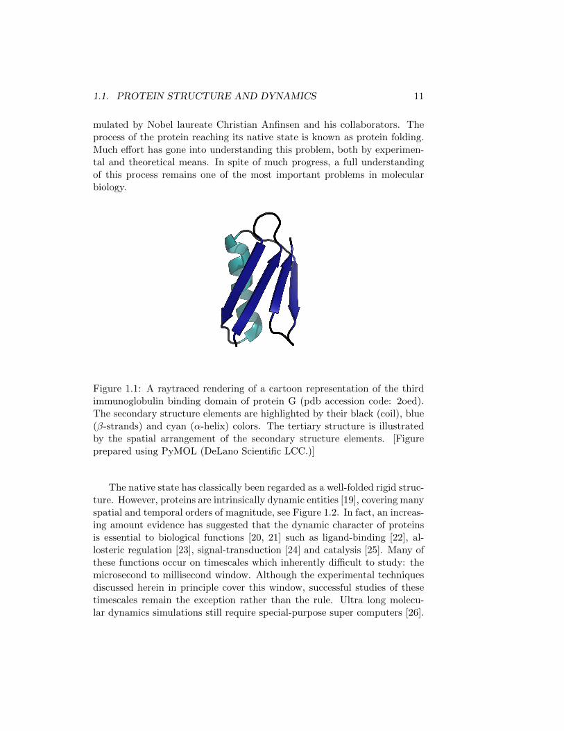
Amino acids are the basic constituents of proteins. There exist 20 com-mon ones, each of which are characterized by the physiochemical propertiesof their side-chains. A protein is formed by a sequence of these joiningto form a linear heteropolymer, through a condensation reaction. The se-quence of amino acids in a protein is commonly referred to as its primarystructure. When put in an aqueous environment many proteins will spon-taneously adapt local (secondary) and non-local (tertiary) structures (seefigure 1.1), while other require the presence of molecular chaperones or co-factors [17, 18]. This observation has lead to the hypothesis that the nativestate is encoded in the primary sequence of amino acids, as originally for-

1.1. PROTEIN STRUCTURE AND DYNAMICS 11

mulated by Nobel laureate Christian Anfinsen and his collaborators. Theprocess of the protein reaching its native state is known as protein folding.Much effort has gone into understanding this problem, both by experimen-tal and theoretical means. In spite of much progress, a full understandingof this process remains one of the most important problems in molecularbiology.

Figure 1.1: A raytraced rendering of a cartoon representation of the thirdimmunoglobulin binding domain of protein G (pdb accession code: 2oed).The secondary structure elements are highlighted by their black (coil), blue(β-strands) and cyan (α-helix) colors. The tertiary structure is illustratedby the spatial arrangement of the secondary structure elements. [Figureprepared using PyMOL (DeLano Scientific LCC.)]

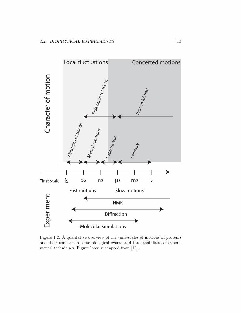
The native state has classically been regarded as a well-folded rigid struc-ture. However, proteins are intrinsically dynamic entities [19], covering manyspatial and temporal orders of magnitude, see Figure 1.2. In fact, an increas-ing amount evidence has suggested that the dynamic character of proteinsis essential to biological functions [20, 21] such as ligand-binding [22], al-losteric regulation [23], signal-transduction [24] and catalysis [25]. Many ofthese functions occur on timescales which inherently difficult to study: themicrosecond to millisecond window. Although the experimental techniquesdiscussed herein in principle cover this window, successful studies of thesetimescales remain the exception rather than the rule. Ultra long molecu-lar dynamics simulations still require special-purpose super computers [26].


In NMR, relaxation dispersion experiments depend on a considerable per-turbation of chemical environment between exchanging states [27] and mayrequire experimental equipment to be pushed to its limits [28]. Alterna-tively, enormous amounts complementary data be acquired and combinedwith simulations [29, 30]. Finally, diffraction experiments provide ratherlow-resolution information, limiting its application to study dynamic eventswhich have substantial spatial rearrangements. Consequently, any progresswhich will make the study of this time window on an atomic more accessiblewill be of great interest.

More recently, proteins apparently devoid of well-defined folds have emerged[31]. These are frequently referred to as intrinsically disordered proteins andtheir functional span in biology is broad [32, 33]. In particular, their flex-ibility has been suggested to be important to function [34]. Some studiessuggest that some of these proteins are well-folded in vivo and suggests thatthe observation of disorder is rather an artifact of in vitro experimentation[35]. While, this may indeed be valid for some particular examples, anypresence of endogenously disordered systems has a significant impact of ourunderstanding of how function arises in structural biology [34].

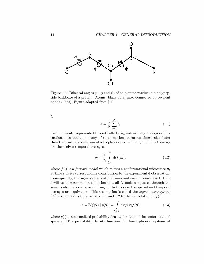
Representing protein structure There are a number of ways to param-eterize protein conformations. For instance may we explicitly represent allN atomic positions as degrees of freedom in the Euclidean space R3N , orthe conformational space. Alternatively, we may use coarse grained repre-sentations, where a reduced set of degrees of freedom aim at representingthe protein – there exists a wide variety of methods to accomplish this [36].One example is to represent the protein by its dihedral angles, φ, ψ and ωfor the backbone (see figure 1.3) and χ-angles for the side-chains [37]. Thisrepresentation allows us to fully reconstruct all atomic positions by assum-ing bond-angles and bond-lengths are constant at some idealized values, forinstance those specified by Engh and Huber [38]. This representation iswhat will be employed throughout this thesis.

1.2 Biophysical experiments

A broad range of biophysical techniques exist to study the structure inbiomolecules. However, due to intrinsic insensitivity of many of these, thesamples studied usually contain a large number N of identical molecules,typically concentrations above those typically expected in vivo. Our ob-served signal, d is thus a spatial average of all the microscopic contributions

1.2. BIOPHYSICAL EXPERIMENTS 13

fs ps ns µs ms s

Vib

rati

on

s o

f b

on

ds

Met

hyl

ro

tati

on

s

Loo

p m

oti

on

Allo

ster

y

Sid

e ch

ain

ro

tati

on

s

Pro

tein

fold

ing

Time scale

Ch

ara

cte

r o

f m

oti

on

Exp

eri

me

nt

Concerted motionsLocal !uctuations

NMR

Di"raction

Molecular simulations

Fast motions Slow motions

Figure 1.2: A qualitative overview of the time-scales of motions in proteinsand their connection some biological events and the capabilities of experi-mental techniques. Figure loosely adapted from [19].


Figure 1.3: Dihedral angles (ω, φ and ψ) of an alanine residue in a polypep-tide backbone of a protein. Atoms (black dots) inter connected by covalentbonds (lines). Figure adapted from [14].

δi.

d =1

N

N∑

i=1

δi (1.1)

Each molecule, represented theoretically by δi, individually undergoes fluc-tuations. In addition, many of these motions occur on time-scales fasterthan the time of acquisition of a biophysical experiment, τe. Thus these δisare themselves temporal averages,

δi =1

τe

τe∫

t=0

dtf(xt), (1.2)

where f(·) is a forward model which relates a conformational microstate xtat time t to its corresponding contribution to the experimental observation.Consequently, the signals observed are time- and ensemble-averaged. HereI will use the common assumption that all N molecule passes through thesame conformational space during τe. In this case the spatial and temporalaverages are equivalent. This assumption is called the ergodic assumption,[39] and allows us to recast eqs. 1.1 and 1.2 to the expectation of f(·),

d = E[f(x) | p(x)] =

∫

x∈χ

dx p(x)f(x) (1.3)

where p(·) is a normalized probability density function of the conformationalspace χ. The probability density function for closed physical systems at


constant temperature is the canonical ensemble [40]

p(x) =exp(−βE(x))

Z(1.4)

where E(·) is the Hamiltonian of the system and β = 1/(kT ) with k is Boltz-manns constant, T is the temperature and Z is the normalization constant,or the partition function. Consequently, biophysical measurements carriedout on bulk solutions are expectations of the forward model with respect tothe canonical ensemble (Boltzmann distribution). The implications of this inthe context of structure and structural ensemble inference will be discussedin section 1.5.

1.2.1 Nuclear magnetic resonance spectroscopy

NMR (Nuclear magnetic resonance spectroscopy) is a versatile biophysi-cal technique which can be used to study system both in, and away from,chemical equilibrium. Thus, the application of NMR may provide a range ofstructural as well as kinetic data. The resolution of the data spans a rangefrom atomic detail to overall shape. This thesis will be exclusively concernedwith data coming from experiments on samples in chemical equilibrium, andthus the discussion herein will be limited to such [41].

In NMR we measure magnetic resonance signals arising when a samplecontaining NMR active nuclei (where spin quantum number S ≥ 1

2) placedin a strong magnetic field, is irradiated by a sequence of radio-frequency(rf) pulses. The pulses perturb the magnetic equilibrium state of the spins.A suitable combination of rf-pulses can isolate a specific phenomenon, re-flecting a specific piece of information. These sequences of rf-pulses arecommonly referred to as pulse sequences or NMR experiments.

The signal acquired following a given pulse sequence is a linear mixtureof complex waveforms, each mixture component corresponds to a nuclei, ina specific physiochemical environment. The signal decays, or relaxes, with arate depending on a broad range of physical effects. This signal is referredto as the free-induction decay, or the FID. In order to distinguish resonancesmore easily, the FID is usually transformed from the time-domain into thefrequency-domain using the Fourier transform, or alternatively maximumentropy and Bayesian reconstruction techniques [42, 43]. This results in anNMR spectrum. In the spectrum, peaks appear at the resonance frequen-cies corresponding to specific nuclei. The resonance frequencies are usuallynormalized to the magnetic field strength and referenced yielding chemicalshifts. Like their corresponding decaying wave-forms, the chemical shifts


are affected by a broad range of physical effects both properties intrinsic tothe nuclear spin and its physical environment. The assignment of peaks toatomic spins typically follows a series of NMR experiments in a procedurewhich may in some cases be automated [44, 45, 46]. This assignment isimportant in most subsequent analyses of the data.

Nuclear Overhauser enhancements

Nuclear Overhauser enhancements (NOEs) are the most important (semi-)quantitative measurements in protein structure inference. Cross relaxationis the physical basis of the NOE. This results from the transfer of magne-tization through dipolar interactions in between excited nuclear spins. Theefficiency of magnetization transfer is inversely related to the inter-atomicdistance as the process is driven by dipolar interactions. Measuring thisprocess therefore yields direct structural information. However, the indirecttransfer of magnetization via other spins (spin diffusion) often hampers theinterpretation of the NOEs. Thus, to extract structural information approx-imations are often used. This effectively results in the semi-quantitativenature of the NOE where the power lies in obtaining a large amount ofimprecise pair-wise distance restraints [41, 47].

The isolated spin-pair approximation (ISPA) is the most widely usedapproach to extract information from NOEs. Here, a pair of spins, in a rigidbody, proximate in space are thought to be isolated and in this way solelyaffecting each others cross-relaxation. This yields a simple relationship (aforward-model) between the NOE, I, and the inter atomic distance, r as

I = γ[r−6] (1.5)

where γ is known as the equilibration parameter, which relates the arbitraryscale of the NOE intensity to a distance scale. The equilibration parametermay either be estimated using a reference experiment [8] or treated as anuisance parameter and subject to statistical inference [7]. A formal deriva-tion of the approximation, and a description of the experimental conditionswhere it is valid may be found elsewhere [8].

More recently some methods have been developed attempting to modelthe contribution of spin diffusion to the NOE using a simulated relaxationmatrix [48] or an auxiliary mean-field spin [49], yielding some more quantita-tive NOEs, facilitating the determination of ensembles of protein structures[50].

Ambiguously assigned NOEs, Ia, often constitute a considerable amountof the available data. Thus it is not exactly known which atomic spin pairs


are giving rise to an observed NOE. However, this information may oftenbe salvaged by considering all possible assignments, A , and simply using a’r−6 summed NOE ’ [51],

Ia = γ

(∑

i∈A

r−6i

). (1.6)

This relationship is of course only valid if the equilibration factor of thedifferent spin pairs is the same – this assumption include a range of physicaleffects, perhaps most significantly that the spin-spin correlation times andorder parameters are identical for all spin-pairs, A .

I stress that the ISPA forward-model is an approximation, and is highlydegenerate. That is, there will be many pairs of γ and r that will yield acorrect NOE – this degeneracy becomes even more pronounced when as-signment of the NOEs is ambiguous. Consequently, these short-comings areideally accounted for when used for structure calculation.

(Residual) dipolar couplings

The residual dipolar coupling (RDC) is another parameter which is measur-able by NMR. From a set of these, we may obtain information about relativeorientational geometry of inter-atomic vectors in the frame of the molecularsystem. In many cases, RDCs may be used for validation or refinement ofdetermined structures [52] or in some cases even structure determination[53].

The geometrical information of the RDCs is averaged on time-scalesup to 100ms. Consequently, any dynamic processes happening on time-scales shorter than this may be uncovered, provided sufficiently accuratemeasurements [54].

A dipolar coupling between spins i and j in a body undergoing rotationaldiffusion is commonly expressed in the laboratory frame, [41]

Dij = Dmax

⟨3 cos2 θij − 1

2

⟩(1.7)

with

Dmax = −µ0γiγjh

8π3r3ij

. (1.8)

θij is the angle between an external magnetic field and the vector betweenspins i and j, rij with length rij . µ0 is the magnetic permittivity of vacuum,γX is the gyromagnetic ratio of nuclei X and h is Plancks constant. This


corresponds to the time-independent form of the secular part of the dipolarinteraction Hamiltonian which approximates the full Hamiltonian well athigh magnetic fields [54]. We have assumed that the bond-length is time-independent.

The laboratory frame is, however, often of limited practical use, as itis difficult to deconvolute the angular average as it depends on a range ofeffects including the internal and overall motions of the molecule and themolecular structure. Consequently, it is often more convenient to expressthe dipolar coupling in the molecular frame of a rigid body,

Dij = DmaxrTijArij. (1.9)

The Saupe, or alignment, tensor, A, is a 3 × 3 traceless matrix with fiveindependent components. It represents the alignment (effective average ori-entation) of the molecule with respect to an external magnetic field [9, 5].

In an isotropic solution, where molecules are allowed to undergo freerotational diffusion, dipolar couplings average to zero. Consequently, themeasurement of RDCs crucially depends on partial alignment, that is, aneffective average orientation of the molecule with respect to the externalmagnetic field. Using a nematic solvent, such as liquid crystals, may yielda partial alignment [55]. Alternatively, systems that spontaneously align inan external magnetic field may be used [56]. I will here limit the discussionto alignment in nematic phase solvents.

The alignment, and therefore also A, is determined by the physiochem-ical properties (e.g. steric and electrostatic) of molecular system as well asinterplay with a nematic solvent. Additionally, the degree of alignment maybe dependent on the concentration of the alignment media. Typically, all ofthese effects are summarized in the alignment tensor. From equation (1.9)it follows that detailed structural characterization depends on an accuratedetermination of A.

Methods for the the determination of alignment tensors can be put into two general groups: data-based and data-free. The data-based methodsinclude the histogram method [57] and tensor fitting procedures (see below)[58]. Many of these procedures may be seen as special cases of a generalprobabilistic framework formulated by Habeck and co-workers [5]. The data-free, methods employ simple physical models of the alignment event andresult in de novo prediction of alignment tensors [60, 61, 62]. However, bothapproaches have their distinctive pros and cons. Data-based methods arephenomenologically motivated, and thus physical realism of the tensor isnot guaranteed – it may however be imposed post hoc. Conversely, data-free


methods are typically mechanistically motivated – however, their predictivepower is typically limited by the precision of the physical models used. Iwill give examples of each of such types of alignment tensor models below.

The Almond-Axelsen tensor The Almond-Axelsen alignment tensormodel is mechanically motivated: it assumes that the hydrodynamic shapeof a molecule is the main contributor to alignment. This assumption hasbeen supported by results in their paper presenting the method [61] and aseries of similar mechanistic tensor models [60, 62]. Unlike the more widelyused method PALES (prediction of alignment from structure) explicit simu-lation of the alignment event is avoided, greatly increasing the computationalefficiency of the method.

Almond and Axelsen exploit that the 3× 3 hydrodynamic (or gyration)tensor,

G =1

N

N∑

i=1

xTi xi (1.10)

of a protein structure, x, situated in its center of mass, shares its eigenbasiswith the alignment tensor, A. While, the eigenvectors of the two matricesare shared, the eigenvalues are not. However, the following relations for theeigenvalues, αi, of A to the eigenvalues, γi, of G were observed to providegood results:

(α1, α2, α3) ∝ (1− δ

2, δ − 1

2,−1

2− δ

2) (1.11)

with,

δ =

√γ2 −√γ3√γ1 −√γ3

(1.12)

where γ1 > γ2 > γ3 and α1 > α2 > α3. Thus, determination of the align-ment tensor reduces to the determination of a gyration tensor, an eigenvaluedecomposition (or similar) and a few matrix-matrix multiplications. Note,that the alignment tensor obtained is only known up to a scaling constant,as absolute degree of alignment is not known.

While the tensor model of Almond and Axelsen is very efficient it doescurrently not allow for modeling of non-steric alignment and is not triviallyextended to do so. One example is when alignment is due to electrostaticinteractions between the alignment-media and the aligning molecule. In thiscase simple steric obstruction does not accurately capture the molecularalignment [62, 63]. However, the lack of generally successful mechanisticmodels of electrostatic alignment, suggests that it is an intrinsically difficultproblem.


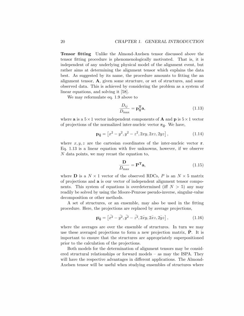
Tensor fitting Unlike the Almond-Axelsen tensor discussed above thetensor fitting procedure is phenomenologically motivated. That is, it isindependent of any underlying physical model of the alignment event, butrather aims at determining the alignment tensor which explains the databest. As suggested by its name, the procedure amounts to fitting the analignment tensor, A, given some structure, or set of structures, and someobserved data. This is achieved by considering the problem as a system oflinear equations, and solving it [58].

We may reformulate eq. 1.9 above to

Dij

Dmax= pT

ija, (1.13)

where a is a 5×1 vector independent components of A and p is 5×1 vectorof projections of the normalized inter-nucleic vector rij. We have,

pij =[x2 − y2, y2 − z2, 2xy, 2xz, 2yz

], (1.14)

where x, y, z are the cartesian coordinates of the inter-nucleic vector r.Eq. 1.13 is a linear equation with five unknowns, however, if we observeN data points, we may recast the equation to,

D

Dmax= PTa, (1.15)

where D is a N × 1 vector of the observed RDCs, P is an N × 5 matrixof projections and a is our vector of independent alignment tensor compo-nents. This system of equations is overdetermined (iff N > 5) any mayreadily be solved by using the Moore-Penrose pseudo-inverse, singular-valuedecomposition or other methods.

A set of structures, or an ensemble, may also be used in the fittingprocedure. Here, the projections are replaced by average projections,

pij =[x2 − y2, y2 − z2, ¯2xy, ¯2xz, ¯2yz

], (1.16)

where the averages are over the ensemble of structures. In turn we mayuse these averaged projections to form a new projection matrix, P. It isimportant to ensure that the structures are appropriately superpositionedprior to the calculation of the projections.

Both models for the determination of alignment tensors may be consid-ered structural relationships or forward models – as may the ISPA. Theywill have the respective advantages in different applications. The Almond-Axelsen tensor will be useful when studying ensembles of structures where

1.3. PROBABILITY THEORY 21

the structural heterogeneity is large where meaningful superpositioning isdifficult [64]. Examples of such may be unfolded protein states or intrinsi-cally disordered proteins – here we may assume that each of the membersof the ensemble align independently and does not change shape during thealignment event [65, 66]. When superpositioning is not needed or no prob-lem, the fitting of tensors may be desirable, in particular when alignment isnon-steric [30].

1.3 Probability theory

From experimental noise and data sparsity arises one of key concepts of theinference problems: uncertainty. The theory of probability provides a nat-ural framework for the quantification of uncertainties [67]. Consequently,the application of probability theory to the problems of inferring proteinstructures and protein structural ensembles from data allows for rigorousassessment of data and models [2]. This section will outline the basic con-cepts essential to probabilistic protein structure inference.

There are two fundamental rules that govern probabilistic models: thesum and product rules. For the variables X and Y , we have:

Sum rule: P (X) =∑Y

P (X,Y )

Product rule: P (X,Y ) = P (X | Y )P (Y ).The summation runs over all possible outcomes of the discrete variable,Y , in a process often referred to as marginalization. Marginalization, orintegrating out, can be generalized to continuous variables (x and y) byreplacing the sum by an integral:

p(x) =

∫

y

dy p(x, y).

The product rule reads: the joint probability of X and Y is equal to theprobability ofX given Y times the probability of Y . Please note, the productrule takes the same form for continuous variables.

Since the probability of X and Y is the same as the probability Y andX, we may use the product rule to obtain,

P (Y | X)P (X) = P (X | Y )P (Y )

which is equivalent to

P (Y | X) =P (X | Y )P (Y )

P (X). (1.17)


This relationship between the conditional probabilities of X and Y is themuch celebrated Bayes’ theorem. In a Bayesian view probabilities quantifyour degrees of belief, and Bayes theorem has a very particular interpretation[68, 67]. For example, let Y be a protein structure and X be some exper-imental data. The conditional probability P (Y | X) is called the posteriorwhich quantifies our belief of a certain protein structure Y having observedour data, X. P (X | Y ), is called the likelihood of the data, X, given a pro-tein structure, Y . Finally, P (Y ) is called the prior distribution of Y , andspecifies our belief, or knowledge, about protein structures (Y ) before hav-ing observed the data (X). The denominator, P (X) is the typically calledthe evidence. Using the sum and product rules, we note the evidence cantake the form

P (X) =∑

Y

P (X | Y )P (Y ),

which is exactly the sum of quantities in the nominator.

While this section has primarily been considering discrete variables, theprinciples discussed also apply to continuous variables.

1.3.1 Bayesian Networks

The process of constructing Bayesian models usually involves repeated ap-plication of the sum and product rules to joint probability functions. Thiscan occasionally lead to intricate expressions which in turn make it difficultto parse out statistical independencies amongst variables. However, it is pos-sible to establish diagrams, or graphs, of probabilistic models. These yield avisualization of the model and determine the independencies of the model.These two properties of graphs may be used to make visual adjustments andexpert assessments, while at the same time formulating the mathematicalmodel [69].

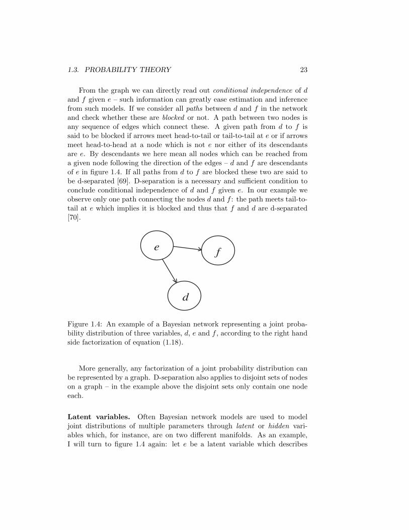
Graphs are composed of two basic components: nodes which representvariables or sets thereof. The nodes are interconnected by edges which repre-sent their statistical relationships. To illustrate Bayesian networks considerthe joint probability function p(d, e, f) of variables d, e and f in the factor-ization

p(d, e, f) = p(d | e)p(f | e)p(e). (1.18)

The corresponding Bayesian network of this factorization is shown in fig-ure 1.4. Each of the variables are represented by a node and for each foreach of the conditional distributions, we add directed edges (arrows) repre-senting the conditioning.


From the graph we can directly read out conditional independence of dand f given e – such information can greatly ease estimation and inferencefrom such models. If we consider all paths between d and f in the networkand check whether these are blocked or not. A path between two nodes isany sequence of edges which connect these. A given path from d to f issaid to be blocked if arrows meet head-to-tail or tail-to-tail at e or if arrowsmeet head-to-head at a node which is not e nor either of its descendantsare e. By descendants we here mean all nodes which can be reached froma given node following the direction of the edges – d and f are descendantsof e in figure 1.4. If all paths from d to f are blocked these two are said tobe d-separated [69]. D-separation is a necessary and sufficient condition toconclude conditional independence of d and f given e. In our example weobserve only one path connecting the nodes d and f : the path meets tail-to-tail at e which implies it is blocked and thus that f and d are d-separated[70].

e

d

f

Figure 1.4: An example of a Bayesian network representing a joint proba-bility distribution of three variables, d, e and f , according to the right handside factorization of equation (1.18).

More generally, any factorization of a joint probability distribution canbe represented by a graph. D-separation also applies to disjoint sets of nodeson a graph – in the example above the disjoint sets only contain one nodeeach.

Latent variables. Often Bayesian network models are used to modeljoint distributions of multiple parameters through latent or hidden vari-ables which, for instance, are on two different manifolds. As an example,I will turn to figure 1.4 again: let e be a latent variable which describes


the relationship between the number of amino-acid residues in a protein (f)and its iso-electric point (d). The parameter f would be modeled using adiscrete multinomial distribution, while the continuous Normal distributionappears appropriate to model d. In this example the latent variable, e,does not have any apparent physical interpretation, but serves to model anycorrelation structure between these two types of experimental data. Theanalysis of the latent variable states often reveal physically sensible features[14, 71]. As the latent variables are unobserved they are to be estimated es-timated from training data using the Expectation-Maximization algorithm(see section 1.3.3).

There are a range of examples of Bayesian network models of structurein biological macromolecules including RNA [72] and proteins [73, 14, 74].These latter models will be discussed below.

1.3.2 Prior distributions

The construction of the prior distribution is one of the key aspects of theBayesian view of probability theory. Ideally, a given prior distribution on aparticular variable should quantify our ignorance about that same variable.Such a prior typically referred to as being non-informative, or ’objective’.In the one-dimensional case there are a number of ways to construct suchpriors including, the principle of maximum entropy (and the related princi-ple of indifference) and Jeffreys principle of invariance. The former readilyapply to discrete variables, in finite intervals, whereas the latter apply tobounded or unbounded one-dimensional continuous variables [75]. This inthis thesis I exclusively work with continuous variables. Consequently, I willonly introduce the concept of the Jeffreys prior.

Jeffreys principle of invariance states that any prior density on a param-eter, θ, should yield an equivalent result if applied to a bijective transforma-tion of that parameter [76]. From this principle, we may get a prior of π(θ)of a one-dimensional parameter θ is given by,

π(θ) ∝√

J (θ) (1.19)

where J (θ) denotes the Fisher information of θ. The Fisher informationis given by,

J (θ) = −∫

x∈χ

dx

[d2

dθ2log p(x | θ)

]p(x | θ) (1.20)

which is exactly minus the expectation of second derivative of the log-likelihood of x given θ with respect to θ. Equation 1.19 may be extended


to construct multidimensional prior distributions – however, the results arethen more controversial [76].

Prior distributions for protein structure

In the opening of the chapter and in section 1.3 I introduced the priordistribution P (Y ) of protein structures, however, no details of its originwas given. I will make extensive use of such priors below, thus the finalpart of this section will introduce a few examples of such. Protein structureis ideally described using a continuous, multidimensional descriptors, forexample all atomic position of the given protein. Thus to conform to mystandard notation, π(x), will from now on refer to prior distribution ofprotein structure.

We may generally classify the existing prior distributions of protein struc-ture in two different classes: mechanically motivated and phenomenologi-cally motivated. The former typically refers to the Boltzmann distribution[π(x) ∝ exp(−βE(x))] of a physical forcefield (E(x) = Epf(x)) based upon,supposedly bona fide physical interactions within a protein [77]. The latter,commonly known as ’knowledge-based potentials’, is based upon learningstatistical models of protein structure using experimentally solved structuresdeposited in the Protein Databank (PDB) [14, 74]. However, the boundarybetween these two classes of model is soft as there exists many examples ofcombinations of these approaches.

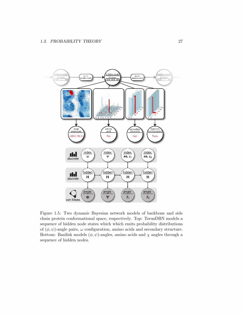
Bayesian network models for protein structure As a pair the knowledge-based probabilistic models, TorusDBN[14] and Basilisk [74], cover the entireprotein conformational space. Both are dynamic Bayesian networks whichessentially corresponds to generalized hidden Markov models. Such modelsare simply Bayesian network models used to model sequential data. Thestrategy in TorusDBN is to model the sequences of amino acids, (φ, ψ)-angle pairs, ω configuration and secondary structure, jointly. This is donealong the backbone yielding a model of local protein structure. Similarly,Basilisk models amino acids, (φ, ψ)-angles and side-chain χ-angles as dy-namic Bayesian network. Both models are summarized in Figure 1.5. Akey strength of these models is the continuous representation of the dihe-dral angles using uni- and bi-variate von Mises distributions: the Normaldistributions on the circle or the torus, respectively. This is is in contrast tothe widely used fragment libraries and rotamer libraries, which effectivelydiscretize the conformational space [78]. Additionally, these models allowfor sampling and conditioning on any of the variables. Thus, if we assume


idealized bond lengths and bond angles we may for example sample proteinstructures with realistic local structure (dihedral angles), given an aminoacid sequence.

Physical forcefields for protein structure As an example of an all-atom protein forcefield I will turn to Profasi, Eprofasi(x). This forcefield isparameterized in torsional space, similarly to TorusDBN and Basilisk – thatis, torsional angles within a protein, such as φ and ψ of the backbone andχ-angles of the sidechain. Thus, to be able to specify all the positions ofatoms geometrical parameters such as bond lengths and bond angles areassumed to be fixed [79]. The mathematical expression for the interactionpotential consists of four terms

Eprofasi(x) = Eloc(x) + Eev(x) + Ehb(x) + Esc(x)

where, Eloc(x), describes local interactions, that is, interactions betweenatoms separated through only a few covalent bonds. The remaining threeterms account for non-local interactions, such as excluded-volume effects(Eev(x)) and hydrogen-bonds (Ehb(x)). Finally, charge-charge and hy-drophobic interactions between sidechains is contained in the term Esc(x).The simplicity of Profasi makes its evaluation extremely fast, and thusamenable for use on non-supercomputers. In spite of the simplicity, theforcefield has been shown to exert physical realism on smaller protein sys-tems.

1.3.3 Expectation Maximization

The Expectation Maximization (EM) algorithm is a general technique toestimate latent variables in statistical models [80]. It can be shown that thealgorithm is guaranteed to yield a maximum likelihood estimate of the latentvariables conditioned on the observed data, even if some data is missing [70].This section will broadly outline the technique.

Let x be a set of experimental observations, h be a set of latent variablesand m represent the missing data. From a Bayesian standpoint there is noconceptual difference between missing data and the unobserved latent vari-ables. Here I will however make the distinction, as it makes the discussionof the EM algorithm more clear.

Now, the EM algorithm proceeds as follows. Firstly, the missing valuesm are filled in using the expected values from p(m | h,x) where h is initial-ized at random. Secondly, the latent variables h are estimating assuming


Figure 1.5: Two dynamic Bayesian network models of backbone and sidechain protein conformational space, respectively. Top: TorusDBN models asequence of hidden node states which which emits probability distributionsof (φ, ψ)-angle pairs, ω configuration, amino acids and secondary structure.Bottom: Basilisk models (φ, ψ)-angles, amino acids and χ angles through asequence of hidden nodes.


the missing data is equal to the expectation from the previous step andmaximizing p(h | x,m). Use the newly estimated h in step 1 and repeat thesequence until convergence [76]. In some cases evaluating the expectation isnot trivial – here a variation of the algorithm called Stochastic EM may beused [81].

Validity and convergence of an EM algorithm can be assess by consid-ering the change in the expected marginal log-likelihood p(x | l,m) as afunction of iteration. A valid algorithm will alway result in a change in thelog-likelihood which is either equal to or larger than zero [80].

1.3.4 Kullback-Leibler divergence

The Kullback-Liebler divergence KL(p | q) is a common measure used tocompare probability distribution functions p(·) and q(·). Although it isnot strictly a distance measure, it is often used as an intuitive analogue.The reason for this is that it does not fulfill the axiomatic requirementsfor a metric – for instance, KL(p | q) 6= KL(q | p) nor is KL(a | c) ≤KL(a | b) + KL(b | c). Rather the divergence more precisely measures theinformation lost when p(·) is approximated by q(·) [82].

For two continuous probability density functions p(·) and q(·) of x theKullback-Liebler divergence is given by,

KL(p | q) =

∞∫

−∞

dx ln

[p(x)

q(x)

]p(x). (1.21)

1.3.5 The reference ratio method

Below I will make use of the so-called reference ratio method (RRM). Thismethod allows for seamless combination of coarse grained information andfine grained information [83, 75]. That is, a probability distribution in a de-tailed representation of a system, for instance a full atomic model of proteinstructure, x, may be combined with a probability distribution of a reducedrepresentation of the same system. For instance, let f(·) be a function whichmaps the fine grained space χ into a reduced space in RN , f : χ→ RN . Thisfunction could for instance be the calculation of the radius of gyration of aprotein structure given its coordinates,

Rg = f(x) =1

M

M∑

i=1

(xi − x)T (xi − x) ∈ R (1.22)

1.4. STATISTICAL SAMPLING IN HIGH-DIMENSIONAL SPACES 29

where xi represent mass-weighed atomic coordinate of atom i and x rep-resents the mass-weighed average atomic position, of the M atoms in theprotein.

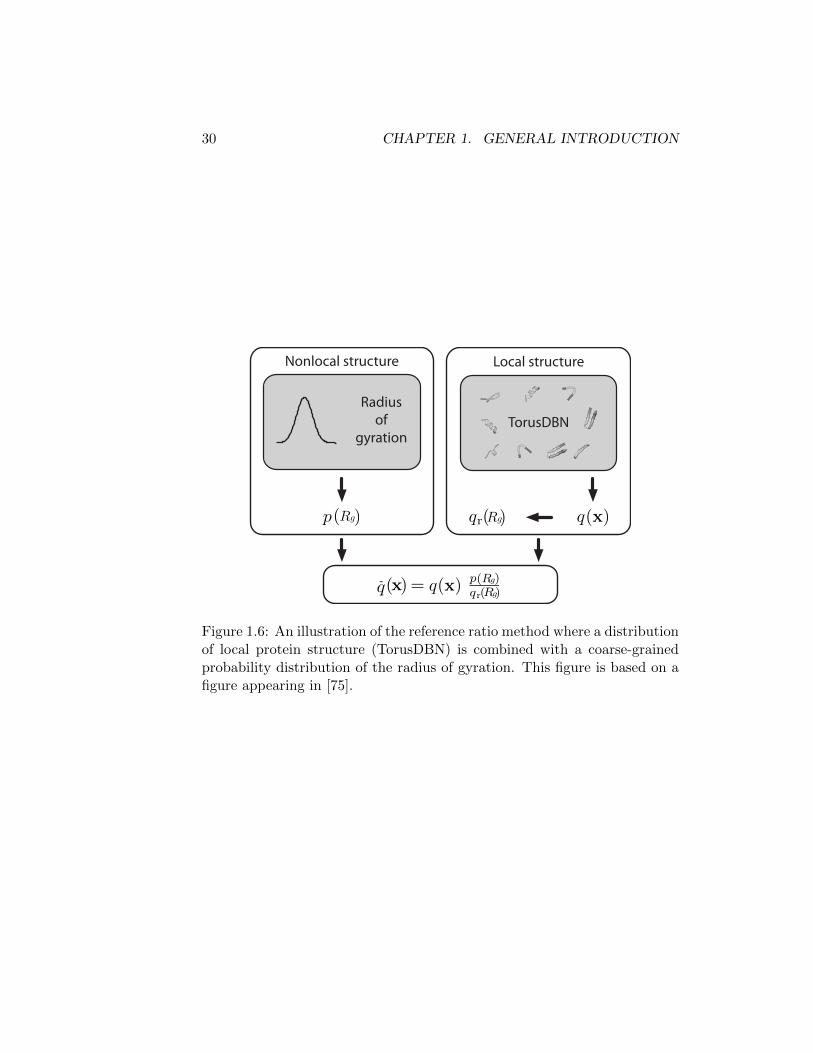
In the following we will assume that we have obtained a probabilitydistribution of the radius of gyration, p(Rg), for instance a knowledge-basedpotential as discussed above. We would like to combine this distribution withsome fine-grained distribution of the conformational space, q(x), to a newdistribution q(x), such that f(q(x)) = p(Rg). The fine-grained distributionsmay for instance be TorusDBN discussed above. The RRM provides theresult,

q(x) = q(x)p(Rg)

qr(Rg)(1.23)

where qr(Rg) is called the reference distribution and is the distribution of Rgaccording to the distribution q(x). Note, that the distribution qr(·) rarely isof a standard form, in particular when more complicated functions for f(·)are considered. Such cases may often be handled through approximationwhich provide sufficiently accurate results. In other cases is the distributionqr(·) is close to uniform ( p(·)qr(·) ≈ p(·)). Here we may safely ignore qr(·) togood approximation.

Although, I’ve here given a simple example from structural bioinformat-ics, the RRM is a general statistical result. Effectively, it yeilds a Kullback-Leibler optimal modification of a distribution, q(·), in the light of a distribu-tion in a transformed space, p(·) [75]. Kullback-Liebler optimality refers tomethods property of minimizing the divergence measure of the original prob-ability distribution q(·) with respect to the resulting one q(·). In informationtheory this corresponds to preserving as much as the original informationas possible and is closely linked to the principle of maximum entropy ofstatistical physics [82].

1.4 Statistical sampling in high-dimensional spaces

The determination of protein structure and protein structural ensembles fre-quently amounts to inference based upon a probability density defined forthe protein system of interest. For instance, a probability distribution of aphysical system may typically be the Boltzmann distribution. The Boltz-mann distribution is defined from mathematical expressions of the potentialenergy of the system – a force field – and specifies the probability of a givenmicro-state, or molecular configuration, x. In the context of inference ofprotein structure and protein structural ensembles, simplistic force fields are


Nonlocal structure Local structure

TorusDBN

Radius

of

gyration

p(R g) q(x )qr (R g)

-q(x) = q(x )p( R g)qr(R g)

Figure 1.6: An illustration of the reference ratio method where a distributionof local protein structure (TorusDBN) is combined with a coarse-grainedprobability distribution of the radius of gyration. This figure is based on afigure appearing in [75].


often combined with expression bringing in experimental observations, in ahybrid energy [1]. These probability distributions are of non-standard formand very high-dimensional: they typically are expressed using all atomicpositions in protein system of interest. Moreover are these distributions of-ten only known up to a normalization constant. For these reasons, directsampling is often infeasible and analytical treatment is generally intractable.

This section introduces a set of methods which allows us to draw sta-tistical samples from such high-dimensional distributions – Markov chainMonte Carlo (MCMC) methods. MCMC methods have a long history inmost branches of quantitative, computational sciences and engineering [84].Samples obtained using an MCMC method facilitate the estimation of nor-malization constants and evaluations of arbitrary expectations, such as ex-perimental observables [3]. In addition, they may be used to determineprotein structures and ensembles of such.

The goal of MCMC methods is to construct a Markov chain which hasthe desired probability distribution as its stationary distribution. A Markovchain is a stochastic process which undergoes transitions in between states.It is characterized by possessing the Markov property: the next state ofthe process depends only on the current state. The Markov property issometimes called ’memorylessness’. Here, I will not distinguish betweendiscrete and general-state space Markov chains, as the results used here areanalogous [84].

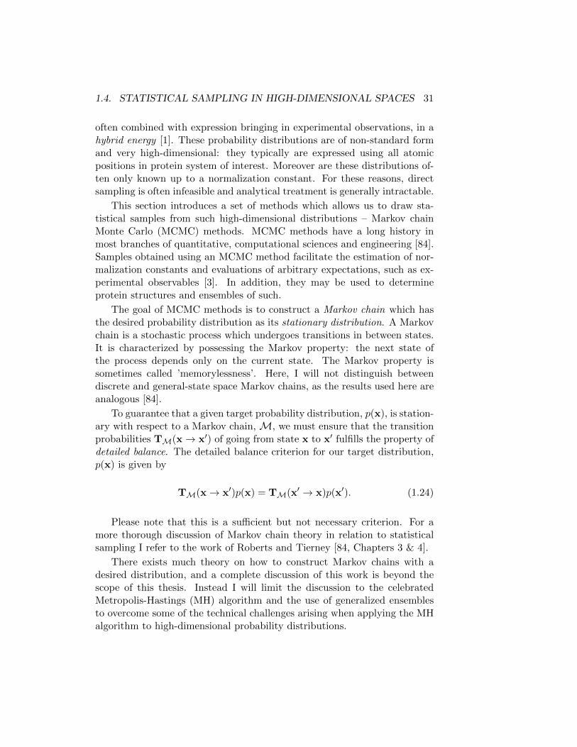
To guarantee that a given target probability distribution, p(x), is station-ary with respect to a Markov chain,M, we must ensure that the transitionprobabilities TM(x→ x′) of going from state x to x′ fulfills the property ofdetailed balance. The detailed balance criterion for our target distribution,p(x) is given by

TM(x→ x′)p(x) = TM(x′ → x)p(x′). (1.24)

Please note that this is a sufficient but not necessary criterion. For amore thorough discussion of Markov chain theory in relation to statisticalsampling I refer to the work of Roberts and Tierney [84, Chapters 3 & 4].

There exists much theory on how to construct Markov chains with adesired distribution, and a complete discussion of this work is beyond thescope of this thesis. Instead I will limit the discussion to the celebratedMetropolis-Hastings (MH) algorithm and the use of generalized ensemblesto overcome some of the technical challenges arising when applying the MHalgorithm to high-dimensional probability distributions.


1.4.1 The Metropolis-Hastings algorithm

While the discussion above may appear terse, it is fortunately simple toconstruct a Markov chain with the desired properties. One of the most well-known algorithms to do this is the Metropolis-Hastings (MH) algorithm.The MH algorithm was formulated by Hastings [85] as a generalization ofthe algorithm proposed by Metropolis and co-workers [86]. Before I proceedto the MH algorithm I will briefly describe the Metropolis algorithm.

The Metropolis algorithm proceeds as follows: given the current state,x, a new state, x′, is proposed from a symmetrical proposal distribution,q(x′ | x): that is, q(x′ | x) = q(x | x′). The new state x′, is acceptedaccording to the Metropolis criteria [86]

U (0, 1) < min

(1,p(x′)p(x)

), (1.25)

where U (0, 1) represents a uniformly distributed number on the unitinterval. If the criterion is not fulfilled the new state is rejected and currentstate is repeated. On the other hand, if the criterion is fulfilled the new statebecomes the current state. We note that the evaluation of the Metropoliscriterion will not require calculation of the normalization constant of thetarget distribution p(·), as it cancels out in the ratio. This may in manycases be convenient as computation of normalization constants is intractablein many complex systems.

The MH algorithm relaxes the requirement of having a symmetrical pro-posal distribution q(x′ | x). This may be done by simply accounting for thebias introduced by the proposal distribution in the Metropolis criterion,

U (0, 1) < min

(1,p(x′)q(x | x′)p(x)q(x′ | x)

). (1.26)

It has been shown that the Metropolis and Metropolis-Hastings algo-rithms indeed fulfill the criterion of detailed balance, and thus generatesamples from the desired target distribution, p(x) [70].

The choice of proposal distributions is application dependent and oftenof decides the efficiency of the algorithm. In particular, in complex problemssuch as protein structure prediction, the curvature of the target probabilitydensity changes drastically as a function of state, yielding general proposaldifficult. Consequently, such simulations often suffer from either low accep-tance or poor mixing. Poor mixing often constitutes to the Markov chain’getting stuck ’ in unrepresentative modes of the target distribution, or highcorrelation in between samples, leading the slow convergence.


1.4.2 Generalized ensembles

There has been a lot of work done to overcome the shortcomings of the MHalgorithm outlined in the section above. One approach is to replace the tar-get distribution, p(x), by a distribution which may be sampled with higherefficiency. The distributions usually chosen based upon their ability increaseconnectivity in between states, which otherwise are poorly connected. Col-lectively, these algorithms are referred to as extended ensembles, and includereplica-exchange Monte carlo or parallel-tempering and the generalized en-sembles. This section will only be concerned with the latter. A thoroughdiscussion of extended ensembles in general can be found elsewhere [87].

The extended ensembles have their origin in statistical physics, it willtherefore be useful to discuss these using the appropriate semantics. Let χbe the state-space of all configurations, x, and let E(·) be a function (anenergy function) which maps this state-space, χ, to a real number – that is,E(·) : χ → R. A probability density function over all states, x ∈ χ, maynow be defined as,

pw(x) =w(E(x))

Zw, Zw =

∫

x∈χ

dxw(E(x)) (1.27)

where w(·) is a weighing function, and Zw is its corresponding partitionfunction. From physics, a classical choice for the weighting function of someenergy, E0, could be w(E0) = exp(−βE0), with the inverse temperature,β = (kT )−1, where k is Boltzmanns constant and T is the temperature.This weighing function corresponds to the Boltzmann distribution, or thecanonical ensemble, introduced previously. We note that any (unnormal-ized) probability density function, p(x), may be expressed in this ensemblewith β = 1 and E0 = − log p(x).

Generalized ensembles rely on a reduced representation of the state-space. That is, instead of parameterizing the state-space as x ∈ χ, a trans-formation is used. One example could be to use an energy, E0, from anenergy function E(x), as introduced above. Using this example, we mayobtain the marginal distribution of the the energy E0 as,

p(E0) =

∫

x∈χ

dxw(E(x))δ(E(x)− E0)

Zw=w(E0)g(E0)

Zw(1.28)

where δ(·) denotes Diracs delta-function and g(E0) =∫

x∈χdx δ(E(x) − E0)

is called the density of states in physics. The density of states, g(E0), may


be interpreted as being a measure of degeneracy of a particular energy, E0.In the generalized ensembles we are still allowed to propose new states usingour proposal distribution from above, q(x′ | x).

The generalized ensembles distinguish themselves from other extendedensemble methods by changing the weighing function, w(E0), the distri-bution of ’energies’ (or − log p(x)) away from the Boltzmann distribution.Typically, the weighing function is chosen as to improve traversal of thestate-space, that is, to facilitate transitions between low- and high-probabilitystates. I will here outline two of the classical weighing functions: the multi-canonical [88] and 1/k ensembles [89].

In the multicanonical ensemble the weight function is chosen in such away as to have a uniform marginal distribution over the energies. This isachieved by using the weighing function,

wGE(E0) =1

g(E0). (1.29)

While this weighing function facilitate transitions in between high and lowprobability regions it may tend to spend much time in low-probability re-gions, of little interest in the context of structure inference. As an alterna-tive, the 1/k-ensemble assigns a smooth distribution over the energies withspecial emphasis on low-energy (high-probability) regions [89]. The weighingfunction is then given by,

w1/k(E0) =

E0∫

−∞

dE g(E)

−1

in this ensemble.

One of the key challenges in using extended ensembles in practice isthat g(E0) is rarely known a priori. This renders it difficult to evaluate theweight function. However, some algorithms have been proposed to overcomethis [90].

1.4.3 Proposal strategies for protein simulations

When simulating high-dimensional probability density functions an appro-priate proposal strategy is essential to sustain reasonable average acceptanceprobabilities. This section will introduce methods which allows us to do thisfor both updating protein conformations, as well as auxiliary parameters.


Gaussian kernel proposals The perhaps simplest strategy to proposenew states of a variable is to naively draw a new state from a uniform dis-tribution. This may in some cases allows for efficient sampling. However,typically it will not, particularly in dense system where even minute changesmay cause large changes in probability. The use of Gaussian kernel distri-butions is a simple, yet effective alternative to this naive strategy. A changeto the current state is proposed using a normal distribution, where the stan-dard deviation may be chosen to optimize the efficiency of the update. Thisapproach has been discussed in the context of updating protein conforma-tion [91] and we used this strategy to sample nuisance parameters in thescientific papers included in this thesis.

We devised a method to adaptively updating the standard deviation ofa given nuisance parameter during the simulation. We make use of thegradient of the ’energy’ of the current state with respect to the parameter,and use it as to optimize the proposal efficiency over the entire span ofthe simulation, while obeying the detailed balance criterion. I provide atechnical derivation of the procedure in section 4.1.

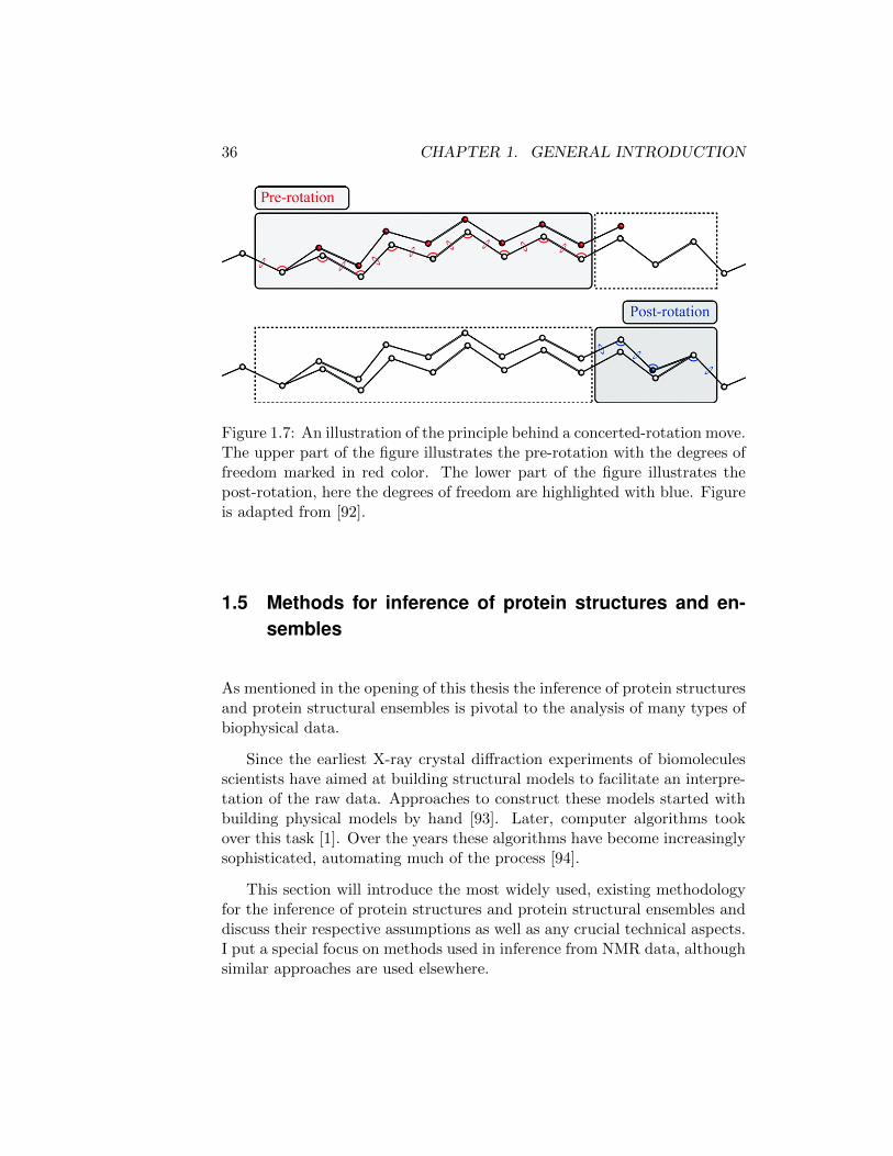
CRISP While the Gaussian kernel strategies generally perform well onthe auxiliary parameters, they still tend to introduce too radical changeswhen applied to protein structures. In particular, when updating dihedralangles, a minute angular change in one dihedral angle may result in dramaticconformational changes downstream. One approach to reduce the impactof an angular update is to split the conformational update into two stepconcerning pre-rotation and a post-rotation, respectively. In this manner aselected local segment of the chain may be selectively updated. The firststep involves a stochastic update of a few angles, while the second deter-ministically restores the local geometry. This is a strategy which has beenextensively employed in a local move type called concerted-rotation [92].

A recent development called CRISP joins the two rotational steps suchthat the pre-rotation explicitly takes into account the deterministic post-rotation. In other words, one constructs a probability distribution over bothpre- and post-rotational degrees of freedom at once, making it possible tosample closed structures while maintaining high quality local geometry. Thisyields more efficient moves which leads to improved sampling, in particularin dense states, such as near native protein conformations [92].


Figure 1.7: An illustration of the principle behind a concerted-rotation move.The upper part of the figure illustrates the pre-rotation with the degrees offreedom marked in red color. The lower part of the figure illustrates thepost-rotation, here the degrees of freedom are highlighted with blue. Figureis adapted from [92].

1.5 Methods for inference of protein structures and en-sembles

As mentioned in the opening of this thesis the inference of protein structuresand protein structural ensembles is pivotal to the analysis of many types ofbiophysical data.

Since the earliest X-ray crystal diffraction experiments of biomoleculesscientists have aimed at building structural models to facilitate an interpre-tation of the raw data. Approaches to construct these models started withbuilding physical models by hand [93]. Later, computer algorithms tookover this task [1]. Over the years these algorithms have become increasinglysophisticated, automating much of the process [94].

This section will introduce the most widely used, existing methodologyfor the inference of protein structures and protein structural ensembles anddiscuss their respective assumptions as well as any crucial technical aspects.I put a special focus on methods used in inference from NMR data, althoughsimilar approaches are used elsewhere.

1.5. INFERENCE OF PROTEIN STRUCTURES AND ENSEMBLES 37

1.5.1 General considerations.

Common to all the methods discussed below is the goal to reach a betterunderstanding of the underlying system that gives rise to our data. We sawin section 1.1 that the data are expectations of the corresponding forwardmodel with respect to the Boltzmann distribution of system. I will hereoutline a few common representations of the Boltzmann ensemble in struc-ture and ensemble inference contexts. I will use d to represent a set of Nexperimental observations {di}Ni=1 when necessary. Similarly, I will use r(x)to for the representations of the corresponding datapoints {f(xi}Ni=1

Representations. In the instantaneous representation, we assume thatthe conformational variation is modest and can be approximated by a singlestate, x′. In eq. 1.3 this corresponds to choosing the Boltzmann distributionequal to the Dirac delta function,

d ≈∫

x∈χ

dx f(x)δ(x− x′) = f(x′). (1.30)

Similarly we may extend this representation to a discrete set of conforma-tions with their respective weights, {xi, wi}Ni=1, that is, a discrete ensemblerepresentation. In this case eq. 1.3 becomes,

d ≈N∑

i=1

wi

∫

x∈χ

dx f(x)δ(x− xi) =

N∑

i=1

wif(xi), (1.31)

whereN∑i=1

wi = 1. These two representations are common in structure and

ensemble inference, respectively. However, these representations intrinsi-cally are approximations. In addition, the forward model may be subjectto approximations and the experimental data subject to uncertainty. Con-sequently, we will not expect a perfect correspondence between the exper-imental data and the back-calculated data. To overcome this error modelsare used.

Error models. Error models consider the discrepancy between experi-mental data and a back-calculated representation, such as those discussedabove. Auxiliary parameters of error models may for instance be an ex-perimental uncertainty or bounds specifying systematic errors. A thorough


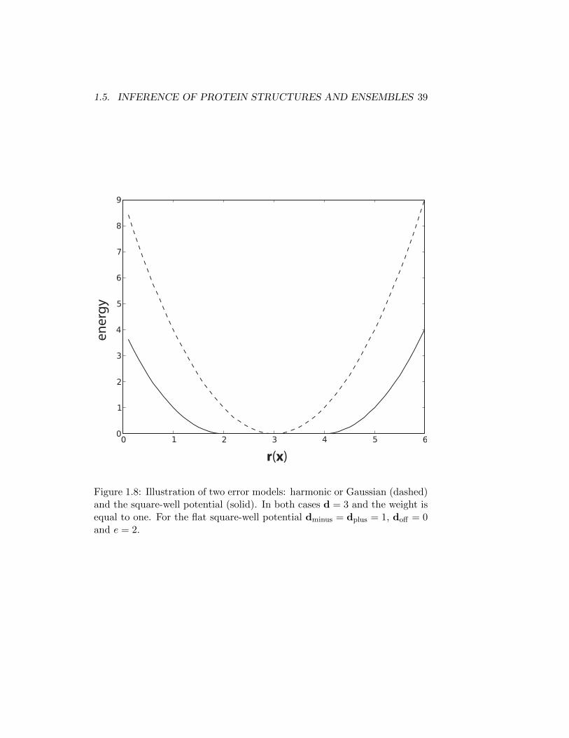
discussion of all error models is beyond the scope of this thesis. However, Iwill here introduce two commonly used ones, see Figure. 1.8.

The harmonic or Gaussian error model is widely used as it only uses asingle auxiliary parameter, the experimental uncertainty. The probabilityof a dataset, d, given a set of representations, r(x), and an experimentaluncertainty, σ may be expressed as

N (d | r(x), σI) =1

(2σπ)N/2exp

[−1

2(d− r(x))T (σ−2I)(d− r(x))

].

(1.32)I is the N ×N identity matrix where N is the number of data points in dand r(x). This error-model is, however, often used in a unnormalized formand expressed as its negated logarithm (corresponding to an ’energy ’),

Eharmonic(x) =

[(d− r(x))

σ

]2

. (1.33)

Thus, we see the energy is a scaled sum of squares.

Another commonly used error-model is called the square-well potential,which may be considered as a generalization of the harmonic potential. Here,bounds define a range of values with the highest probability, unlike themodel above where this value is unique. The error-model is referred to asa potential, as it is formulated as an ’energy’ (− log probability) primarily.The expression for the square-well potential is given by [13],

Esqwell = w∆e (1.34)

where ∆ is given by:

∆ =

r(x)− (d + dplus − doff) if d + dplus − doff < r(x)0 if d− dminus < r(x) < d + dplus − doff

d− dminus − r(x) if r(x) < d− dminus

(1.35)where dminus,dplus and doffset are parameters specifying the bounds of theflat bottom, and e is a parameter specifying the steepness of the potentialwhen outside these bounds. Finally, w is an overall scale of the potential,which is w = σ−2, above [95]. The square-well potential is typically usedwhen only bounds of values are obtained from experiments. For instance,NOEs data is often cast into a number of classes based upon the intensityof the signal. Subsequently these classes are associated with some distancebounds.


r(x)

energy

Figure 1.8: Illustration of two error models: harmonic or Gaussian (dashed)and the square-well potential (solid). In both cases d = 3 and the weight isequal to one. For the flat square-well potential dminus = dplus = 1, doff = 0and e = 2.


1.5.2 Hybrid energy minimization heuristics

Experimental evidence, as for instance the NOE and RDC restraints dis-cussed above, is always complemented by some prior, as even very densedata-sets have insufficient information to calculate the three-dimensionalstructures. Classically, this has been achieved by employing empirical forcefields Eemp(x) [96, 97], akin to Profasi presented above, to complement anenergy derived from the experimental data as introduced in the previoussection. We get a hybrid energy

Ehybrid(x) = wEdata(x) + Eemp(x) (1.36)

where w is the scale parameter which weighs the experimental evidencerelative to the empirical forcefield. This general form of the hybrid energy isubiquitous. However, many different flavors of both Edata(x) and Eemp(x)exists, as discussed previously. In a Bayesian view, this corresponds tohaving different models for the likelihood (Edata) and prior distributions(Eemp).

Similar to a likelihood, the data-energy measures the agreement betweena candidate representation of a system, and some observed experimentaldata. For example, in the case of structure determination from NOEs (seesection 1.2.1) an experimentally observed NOE is related to an instanta-neous pair-wise distance in x, through the forward model ISPA. The betterthe agreement, the lower the error-model energy (or, the higher the proba-bility). The weight, w, is typically adjusted such that the agreement of theexperimental data is within some expected experimental uncertainty. Nui-sance parameters, such as the equilibration constant γ in the ISPA forwardmodel of NOE intensities are often fixed to empirical point estimates [8].

Inference from such models is predominantly done through minimizationof eq. 1.36. In this context, the hybrid energy is seen as a representation ofthe free-energy of the protein. The minimization is then a straightforwardapplication of Anfinsens ’thermodynamic hypothesis’ where the native stateof a protein is thought to be the unique conformation that minimizes thefree energy of the system. Again, many methods exist to perform this min-imization including Monte Carlo and molecular dynamics method (in bothcartesian and angular coordinates) typically combined with a simulated an-nealing heuristic [98, 13, 99]. During the minimization, scheduling schemesallow for gradual adjustment of auxiliary parameters. Typically, the meth-ods are applied in an iterative manner; adjustments to other parameterssuch as peak-assignments are carried out in between trial minimizations.


It is common practice to repeat the minimization multiple times to en-sure consistent structures are obtained. A set of structures (a bundle) isselected for publication. However, a series of validation and refinement pro-tocols are typically employed before this happens [100, 101, 102, 103].

Ensemble minimization and refinement As mentioned at the start,experimental data obtained from biomolecules in solution is often subjectto temporal and spatial averaging. Thus the experimental data may bemore appropriately represented by a discrete ensemble. This correspondsto changing the representation of the Boltzmann ensemble from an in-stantaneous one to a weighed average of a set of N > 1 conformations.This approach emerged more than twenty years ago and remains popular[104, 105, 106, 107, 108, 109, 50]. The type of hybrid energies used in theseapproaches may be trivially derived from general considerations discussedabove. I will return to the subject of modeling ensembles in section 1.5.4below.

The energy minimization heuristics have a number of advantages, pri-marily of a technical or practical nature. The methods are by far the mostwidely used and consequently have been optimized and tested extensively –in particular single conformer techniques. Additionally, many benchmarksand tests have been carried out comparing the results of different imple-mentations and methods. However, these methods generally suffer from anumber of important shortcomings. Firstly, there is no systematic way todeal with the auxiliary parameters such as the weight and the NOE equilibra-tion constant. Consequently, these values are often fixed to empirical pointestimates which in addition to empirical bias does not allow for handling ofpotential uncertainties. In a rigorous application, experimental data shouldbe left out to cross-validate obtained structures and parameters. However,in cases where data is sparse, this may prohibit structure determination alltogether. Secondly, minimization typically underestimates the degeneracyof the hybrid energy as it inherently aims at finding a unique optimal solu-tion [110, 111, 112]. This in turn makes it difficult to assess the precisionand validity of the obtained bundles or ensembles in an objective way [2].

1.5.3 Inferential structure determination

Inferential structure determination aims at putting structure determinationinto a full Bayesian probabilistic framework [2]. That is, to formulate aposterior distribution of structures x and auxiliary parameters n, given the


observed data d and prior information I ,

p(x,n | d, I) ∝ p(d | x,n, I)π(x | I)π(n | I). (1.37)

If we take the negated logarithm of this posterior probability distribution weimmediately obtain an expression analogous to the hybrid energy shown ineq. 1.36 – however, an additional term emerges that accounts for the priorof the auxiliary parameters.

As an illustration I will here give a the posterior distribution for struc-ture inference from NOEs. The likelihood is a combination of a log-normaldistribution (the distribution of a variable whose log is Normal distributed)to model the error of distances, or intensities, and an instantaneous rep-resentation using the ISPA forward model. This introduces two auxiliary,or nuisance, parameters: the equilibration parameter γ and experimentaluncertainty σ. We have, p(d | x,n, I) = log N (d | f(x, γ), σ), where thefunction f(·) is ISPA and n = {γ, σ}. Now we only need to specify the priorsof the parameter-space of x, γ and σ. For x we may chose any structuralprior, for instance one of those discussed above. Similarly, for γ and σ wemay chose any suitable prior. In ISD the simple improper priors π(γ) ∝ γ−1

and π(σ) ∝ σ−1 were used. The priors on the nuisance parameters put spe-cial emphasis on small values and are defined on R+ only, which is compliantwith the domain of the parameters. Both of these priors are referred to asJeffreys priors in original manuscript.

Like hybrid energies, the negative log of the posterior may also be subjectto minimization. This was done on a large-scale recently [113]. However, car-rying out the minimization in this case will have similar drawbacks as thoseoutlined above. Instead, Nilges and co-workers carried out statistical infer-ence by sampling from the posterior distribution using extended ensembleMCMC techniques [114, 2]. In this manner, marginal posterior probabilitydistributions are obtained directly. These allows for direct objective assess-ment of validity, precision and quality of the obtained structures, throughwell-established statistical tests. Similarly, may statistical assessments re-garding the nuisance parameters σ and γ be made. Such properties havelong been lacking in the protein structure determination from NMR data.

1.5.4 Restrained molecular simulations

The methodology discussed above focuses on refining single structure mod-els to agree with experimental data while fulfilling basic prior knowledge ofbiomolecules. This may be a reasonable first approximation for some sys-tems, however, it will be too crude for other, perhaps even the majority


of cases. In fact, the motion in biomolecules has long been recognized tobe one of the key sources of systematic errors in models subject to suchassumptions, as touched upon above [4, 1, 115].

In other contexts, methods have been developed to directly infer theprobability densities of the geometrical properties represented in experi-mental observations [116, 117] – however, these require that complete in-formation of all degrees of freedom is represented in the data. This is veryrare when biological macromolecules are considered. I will here discuss analternative approach where the incomplete information from experimentalobservations is complemented by structural prior information as embodiedeither in forcefields or knowledge-based potentials. Similar to the structuredetermination and refinement techniques above hybrid energy potentials areconstructed as to ensure agreement with experimental data. However, in-stead of minimization the goal is to simulate samples from the underlyingdistribution and thus obtaining a representation of the accessible conforma-tional states [118, 119, 64, 63].

For completeness, I will give an example of a data energy where an N -conformer representation with uniform weights is combined with a reducedharmonic error-model,

Emc−data(x) =

[1N

N∑i=1

f(xi, θi)− d

]2

σ2(1.38)

with θ being the nuisance parameters associated with the forward modelf(·). Note, it is common to multiply this restraining term by N to keep themagnitude of the restraining force approximately independent of N [120].

Recently, Pitera and Chodera presented a different approach to restrain-ing molecular simulations through the principle of maximum entropy [120].In this manner, they obtained a potential which takes the ensemble natureof the data into account, without introducing the notion of multiple repli-cas. For a single experimental observation without experimental uncertainty,they arrived at the hybrid energy,

Ehybrid−pc(x) = αf(x) + Eemp(x) (1.39)

where α is a constant which may be estimated such that the expectation

of f(x) according toexp(−βEhybrid−pc(x))

Z is equal to the experimental data d.They describe a procedure to achieve this in their manuscript. They furtherdemonstrate that the method works well on a one dimensional example inabsence of experimental uncertainty. Finally, they show that their potential


is closely related to eq. 1.38 in the limit where N goes to infinity. A similarresult was recently reported by others [121].

Another approach represents the data by an average of structures alongthe simulation trajectory [122, 123]. However, this approach has a numberof intrinsic limitations and a thorough discussion is thus beyond the scopehere.

1.5.5 Post hoc ensemble selection

The final class of methods i will consider here are the post hoc ensembleselection techniques. The methods emerged less than ten years and ago andhas since then been used predominantly to refine ensembles obtained fromknowledge-based statistical coil libraries to agree with experimental dataof intrinsically disordered proteins [124, 65]. In these methods, a pool of Kstructures is sampled using either statistical coil models or high-temperaturemolecular dynamics simulations. Subsequently, either the pool is weighed[125], a subset of the pool is selected [126, 127] or a combination of these(Olsson, Unpublished work). This is done to optimize the agreement withexperimental data. Through an increasing number of auxiliary heuristicmodifications of forward models [128], these methods now provide excellentagreements to experimental data using a relatively small number of confor-mations [129, 130].

1.5.6 Analysis of methodology

In the previous section I’ve given a brief outline of common methods instructure and structural ensemble determination. This final part is devotedto comparing and analyzing the methods in more detail.

Reference ratio distribution In all of the methodologies introducedabove, the aim is to infer conformational models in atomic detail. However,the experimental data we observe only reflect some projection of the actualunderlying distribution of conformations. Consequently, when we use con-formational prior information to account for the incomplete information, wealso induce prior on the manifold of the data (section 1.3.5). This prior mayin some cases be both strong and inappropriate, and can have a strong neg-ative influence on the posterior distribution. This topic is discussed furtherin section 2.2.


Structure inference There are three key assumptions common to all themethods for protein structure determination presented here. Firstly, theforward-model accurately describes the relationship between a conforma-tional state and its contribution to the experimental data. Secondly, thesingle conformer representation of the Boltzmann distribution is a good ap-proximation. Finally, all experimental observations are uncorrelated andhave equal uncertainty. While the two first assumptions have been widelydiscussed in the literature and consequently also in this thesis, the final onehas not.

It is often convenient to assume that experimental data are uncorre-lated and have equal variance. We assume this about data used for proteinstructure inference. This assumption is most apparent if we consider theharmonic error-model eq. 1.32. Here, we chose a diagonal covariance ma-trix with one variance σ2 common to all diagonal elements. This in turnreduces to a single weighing factor of the sum of square distances betweenthe forward-model and the experimental data. This is completely analogousin the square-well and other closely related potentials. Following the Gauss-Markov theorem this will result in the best linear unbiased estimate if andonly if the data indeed fulfills these assumptions [131]. It is reasonable tosuggest that this is not the case: for instance, sets of NOEs observed betweenadjacent atomic pairs may be highly correlated. The potential consequenceof this includes over-confident wrong structural models.

It appears, however, that such problems have been overcome in practiceby using strong conformational priors in subsequent refinement procedures[100]. In spite of this, it might be an interesting future endeavor to investi-gate if proper handling of the correlation between observations improves thequality of structural models and perhaps alleviates the need for subsequentprocessing. This may be achieved by replacing the diagonal matrix, (σ−2I),from eq. 1.32 with a full covariance matrix.

Unlike the minimization heuristics, inference through sampling of theposterior distribution was reported to be very computationally intensive –it requires a computer clusters of 50 computers to run for a number ofdays. Since such computational demands are excessive for most experi-mental labs, the application of ISD has been limited. Consequently, a moreefficient implementation may stimulate more experimental labs to adapt thismore rigorous methodology. We have proposed a new implementation, seesection 2.1.


Restrained simulations In addition to the assumption made above con-cerning the accuracy of the forward-model similar assumptions regardingthe representation and lack of correlations between observations.

It has been suggested that the discrete representation of the conforma-tional distribution is sufficiently accurate to capture anisotropic motion, inparticular when only very fast motions are represented in the data [132].However, a recent paper demonstrated that measurable bias is introducedwhen discrete ensembles are employed [121]. This may to a large extend bealleviated by using a large number of conformations in the representation.However, it remains an inherent problem that the number of replicas needto be estimated – and most of all there is currently no systematic way tomake this decision or account for its uncertainty. While cross-validation mayprovide a sensible approach to make this assessment it is generally undesir-able for reasons mentioned above. This problem may become more apparentwith increasingly accurate and dense datasets of experimental data averagedover long time scales, as for instance residual dipolar couplings. Similarly,when intrinsically disordered proteins are studied, the anisotropic natureof the conformational ensemble may become quite significant which mayrequire the number of conformations necessary to become computationallyintractable. Consequently, the need for methods that allow restraining thesesimulations which are independent upon discretizations is desirable.

Cavalli and co-workers provided a nice proof of the validity of the usingexperimental uncertainties in the cases of multiple replica restraining poten-tial [121]. However, the replica independent maximum entropy formulationshown by Pitera and Codera as well as Cavalli and co-workers does notexplicitly handle experimental uncertainty. Consequently, any uncertaintyin the data will affect the estimated α or λ parameters. In section 2.2 wediscuss one possibility of how to overcome this shortcoming.

In multiple replica restrained simulation we assume, as in structure de-termination, the observations to be uncorrelated. This is not immediatelyobvious, however, it becomes evident if we consider the continuous case pre-sented by Pitera and Chodera for N datapoints. In that case, a parameterαi for each representation fi(x) of a datapoint i is introduced. We get,

Ehybrid−pc2(x) = Eemp(x) +

N∑

i=1

αifi(x) (1.40)

this is equivalent to

p(x) ∝ exp(−Eemp(x))

N∏

i=1

exp(−αifi(x)) (1.41)


which in statistics corresponds to a generalized linear model of exponen-tial response data also called a log-linear model [133]. The form of themodel given in eq. 1.41 assumes the variables fi(·) to be uncorrelated. As instructure determination, this assumptions will have an effect on the resultsobtained – it is, however, unclear how severe this will be. Still, the currentliterature does address such potential short comings.

Post hoc ensemble selection This class of methods has had much suc-cess, in particular for determining ensembles of intrinsically disordered pro-teins. However, in addition to the assumptions discussed above they havea number of undesirable properties. First, the resulting explicit ensemblesfrom these methods are not unique and easily complement each other. Sec-ondly, since the sampled pool is typically obtained from rather crude modelsit is not always clear whether selected conformations represent any physicalrealism or simply optimize the fit to the experimental data. These short-comings in general limit the practical use of explicit ensemble models.

These ensemble weighing or selection techniques may however be usefulfor averaged data from approximately discrete systems. For instance mix-tures of monomeric and oligomeric forms of proteins. The data available forsuch systems is often rather coarse-grained, eg. small angle X-ray scattering.Consequently, in such cases using atomic-detail molecular simulations maynot only be computationally expensive but also excessive.

Throughout this introduction I have mapped out different fields andtheir methodologies relevant to inference problems in structural biology fromNMR data. In this final section I have discussed out some of the currentproblems and shortcomings in existing methodology – the research paperspresented next addresses some of these.

Cited Literature

[1] Brunger, A. T. and Nilges, M. Quarterly Reviews of Biophysics 26,49–125 1 (1993).

[2] Rieping, W., Habeck, M., and Nilges, M. Science 309(5732), 303–306Jul (2005).

[3] Habeck, M. J. Struct. Biol. 173(3), 541 – 548 (2011). Combiningcomputational modeling with sparse and low-resolution data.

[4] Jardetzky, O. Biochim. Biophys. Acta 621(2), 227 – 232 (1980).

[5] Habeck, M., Nilges, M., and Rieping, W. J. Biomol. NMR 40(2),135–144 Feb (2008).

[6] Habeck, M., Rieping, W., and Nilges, M. J. Magn. Reson. 177(1),160–165 Nov (2005).

[7] Rieping, W., Habeck, M., and Nilges, M. J. Am. Chem. Soc. 127(46),16026–16027 Nov (2005).

[8] Gronenborn, A. M. and Clore, G. Prog. Nucl. Magn. Reson. Spectrosc.17(0), 1 – 32 (1985).

[9] Saupe, A. and Englert, G. Phys. Rev. Lett. 11, 462–464 Nov (1963).

[10] Karplus, M. The Journal of Chemical Physics 30(1), 11–15 (1959).

[11] Svergun, D., Barberato, C., and Koch, M. H. J. Journal of AppliedCrystallography 28(6), 768–773 Dec (1995).

[12] Debye, P. Annalen der Physik 351(6), 809–823 (1915).

[13] Schwieters, C., Kuszewski, J., Tjandra, N., and Clore, G. J. Magn.Reson. 160, 66–74 (2003).

49

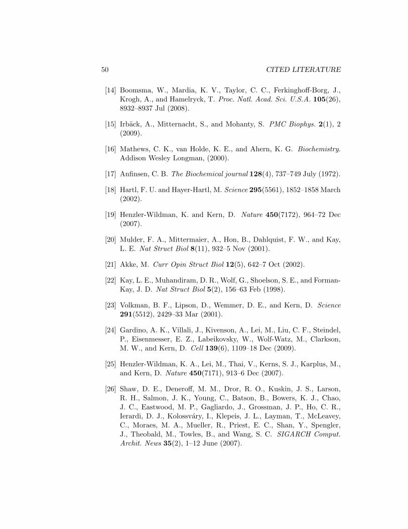
50 CITED LITERATURE

[14] Boomsma, W., Mardia, K. V., Taylor, C. C., Ferkinghoff-Borg, J.,Krogh, A., and Hamelryck, T. Proc. Natl. Acad. Sci. U.S.A. 105(26),8932–8937 Jul (2008).

[15] Irback, A., Mitternacht, S., and Mohanty, S. PMC Biophys. 2(1), 2(2009).

[16] Mathews, C. K., van Holde, K. E., and Ahern, K. G. Biochemistry.Addison Wesley Longman, (2000).

[17] Anfinsen, C. B. The Biochemical journal 128(4), 737–749 July (1972).

[18] Hartl, F. U. and Hayer-Hartl, M. Science 295(5561), 1852–1858 March(2002).

[19] Henzler-Wildman, K. and Kern, D. Nature 450(7172), 964–72 Dec(2007).

[20] Mulder, F. A., Mittermaier, A., Hon, B., Dahlquist, F. W., and Kay,L. E. Nat Struct Biol 8(11), 932–5 Nov (2001).

[21] Akke, M. Curr Opin Struct Biol 12(5), 642–7 Oct (2002).

[22] Kay, L. E., Muhandiram, D. R., Wolf, G., Shoelson, S. E., and Forman-Kay, J. D. Nat Struct Biol 5(2), 156–63 Feb (1998).

[23] Volkman, B. F., Lipson, D., Wemmer, D. E., and Kern, D. Science291(5512), 2429–33 Mar (2001).

[24] Gardino, A. K., Villali, J., Kivenson, A., Lei, M., Liu, C. F., Steindel,P., Eisenmesser, E. Z., Labeikovsky, W., Wolf-Watz, M., Clarkson,M. W., and Kern, D. Cell 139(6), 1109–18 Dec (2009).

[25] Henzler-Wildman, K. A., Lei, M., Thai, V., Kerns, S. J., Karplus, M.,and Kern, D. Nature 450(7171), 913–6 Dec (2007).

[26] Shaw, D. E., Deneroff, M. M., Dror, R. O., Kuskin, J. S., Larson,R. H., Salmon, J. K., Young, C., Batson, B., Bowers, K. J., Chao,J. C., Eastwood, M. P., Gagliardo, J., Grossman, J. P., Ho, C. R.,Ierardi, D. J., Kolossvary, I., Klepeis, J. L., Layman, T., McLeavey,C., Moraes, M. A., Mueller, R., Priest, E. C., Shan, Y., Spengler,J., Theobald, M., Towles, B., and Wang, S. C. SIGARCH Comput.Archit. News 35(2), 1–12 June (2007).

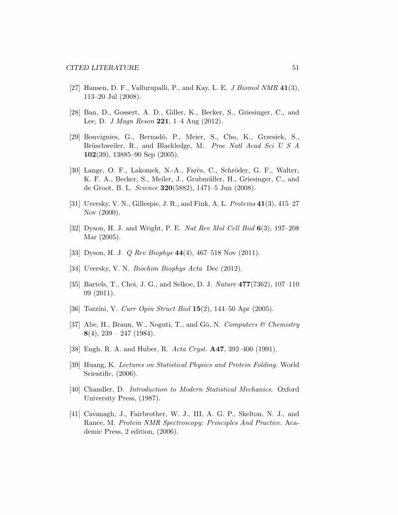
CITED LITERATURE 51

[27] Hansen, D. F., Vallurupalli, P., and Kay, L. E. J Biomol NMR 41(3),113–20 Jul (2008).

[28] Ban, D., Gossert, A. D., Giller, K., Becker, S., Griesinger, C., andLee, D. J Magn Reson 221, 1–4 Aug (2012).

[29] Bouvignies, G., Bernado, P., Meier, S., Cho, K., Grzesiek, S.,Bruschweiler, R., and Blackledge, M. Proc Natl Acad Sci U S A102(39), 13885–90 Sep (2005).

[30] Lange, O. F., Lakomek, N.-A., Fares, C., Schroder, G. F., Walter,K. F. A., Becker, S., Meiler, J., Grubmuller, H., Griesinger, C., andde Groot, B. L. Science 320(5882), 1471–5 Jun (2008).

[31] Uversky, V. N., Gillespie, J. R., and Fink, A. L. Proteins 41(3), 415–27Nov (2000).

[32] Dyson, H. J. and Wright, P. E. Nat Rev Mol Cell Biol 6(3), 197–208Mar (2005).

[33] Dyson, H. J. Q Rev Biophys 44(4), 467–518 Nov (2011).

[34] Uversky, V. N. Biochim Biophys Acta Dec (2012).

[35] Bartels, T., Choi, J. G., and Selkoe, D. J. Nature 477(7362), 107–11009 (2011).

[36] Tozzini, V. Curr Opin Struct Biol 15(2), 144–50 Apr (2005).

[37] Abe, H., Braun, W., Noguti, T., and Go, N. Computers & Chemistry8(4), 239 – 247 (1984).

[38] Engh, R. A. and Huber, R. Acta Cryst. A47, 392–400 (1991).

[39] Huang, K. Lectures on Statistical Physics and Protein Folding. WorldScientific, (2006).

[40] Chandler, D. Introduction to Modern Statistical Mechanics. OxfordUniversity Press, (1987).

[41] Cavanagh, J., Fairbrother, W. J., III, A. G. P., Skelton, N. J., andRance, M. Protein NMR Spectroscopy: Principles And Practice. Aca-demic Press, 2 edition, (2006).

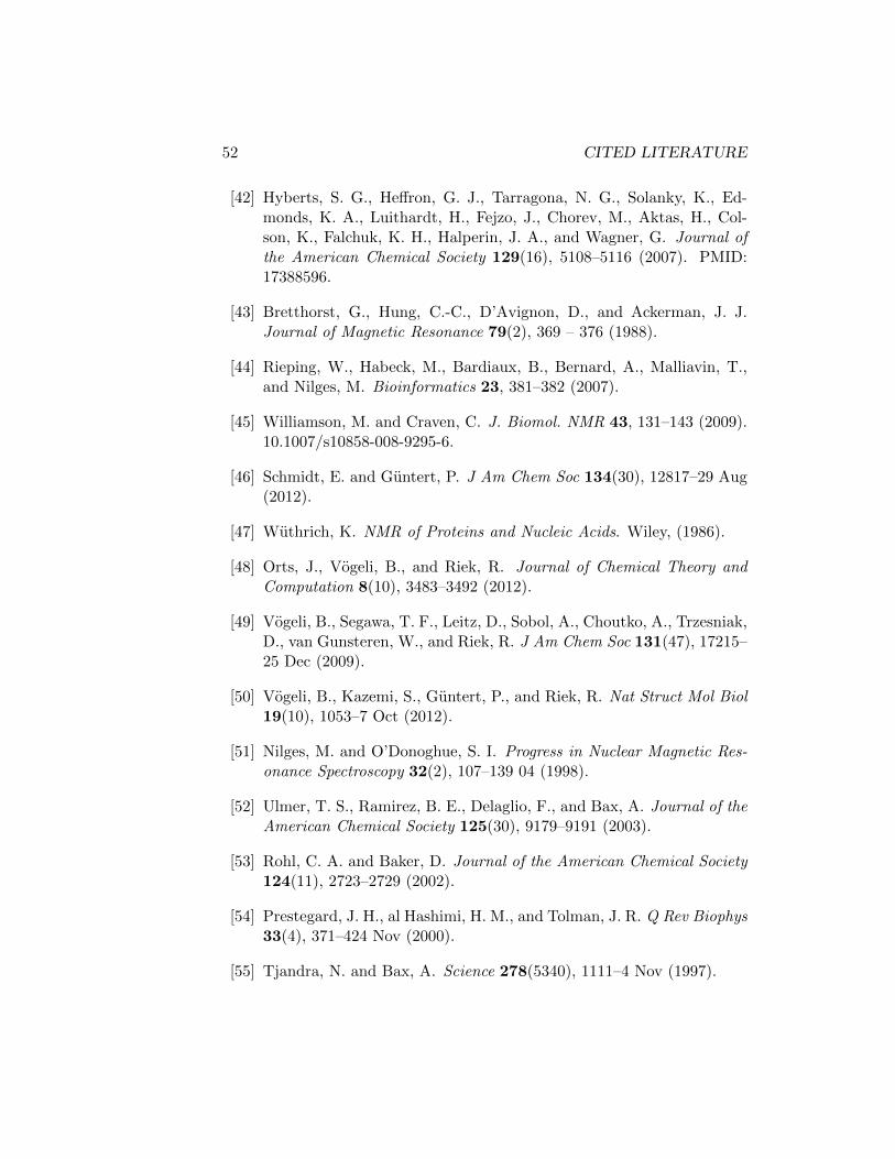
52 CITED LITERATURE

[42] Hyberts, S. G., Heffron, G. J., Tarragona, N. G., Solanky, K., Ed-monds, K. A., Luithardt, H., Fejzo, J., Chorev, M., Aktas, H., Col-son, K., Falchuk, K. H., Halperin, J. A., and Wagner, G. Journal ofthe American Chemical Society 129(16), 5108–5116 (2007). PMID:17388596.

[43] Bretthorst, G., Hung, C.-C., D’Avignon, D., and Ackerman, J. J.Journal of Magnetic Resonance 79(2), 369 – 376 (1988).

[44] Rieping, W., Habeck, M., Bardiaux, B., Bernard, A., Malliavin, T.,and Nilges, M. Bioinformatics 23, 381–382 (2007).

[45] Williamson, M. and Craven, C. J. Biomol. NMR 43, 131–143 (2009).10.1007/s10858-008-9295-6.

[46] Schmidt, E. and Guntert, P. J Am Chem Soc 134(30), 12817–29 Aug(2012).

[47] Wuthrich, K. NMR of Proteins and Nucleic Acids. Wiley, (1986).

[48] Orts, J., Vogeli, B., and Riek, R. Journal of Chemical Theory andComputation 8(10), 3483–3492 (2012).

[49] Vogeli, B., Segawa, T. F., Leitz, D., Sobol, A., Choutko, A., Trzesniak,D., van Gunsteren, W., and Riek, R. J Am Chem Soc 131(47), 17215–25 Dec (2009).

[50] Vogeli, B., Kazemi, S., Guntert, P., and Riek, R. Nat Struct Mol Biol19(10), 1053–7 Oct (2012).

[51] Nilges, M. and O’Donoghue, S. I. Progress in Nuclear Magnetic Res-onance Spectroscopy 32(2), 107–139 04 (1998).

[52] Ulmer, T. S., Ramirez, B. E., Delaglio, F., and Bax, A. Journal of theAmerican Chemical Society 125(30), 9179–9191 (2003).

[53] Rohl, C. A. and Baker, D. Journal of the American Chemical Society124(11), 2723–2729 (2002).

[54] Prestegard, J. H., al Hashimi, H. M., and Tolman, J. R. Q Rev Biophys33(4), 371–424 Nov (2000).

[55] Tjandra, N. and Bax, A. Science 278(5340), 1111–4 Nov (1997).

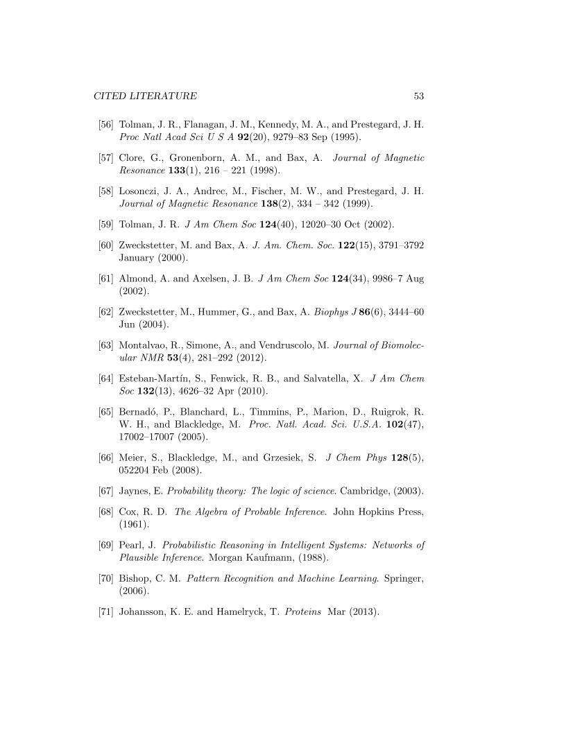
CITED LITERATURE 53

[56] Tolman, J. R., Flanagan, J. M., Kennedy, M. A., and Prestegard, J. H.Proc Natl Acad Sci U S A 92(20), 9279–83 Sep (1995).

[57] Clore, G., Gronenborn, A. M., and Bax, A. Journal of MagneticResonance 133(1), 216 – 221 (1998).

[58] Losonczi, J. A., Andrec, M., Fischer, M. W., and Prestegard, J. H.Journal of Magnetic Resonance 138(2), 334 – 342 (1999).

[59] Tolman, J. R. J Am Chem Soc 124(40), 12020–30 Oct (2002).

[60] Zweckstetter, M. and Bax, A. J. Am. Chem. Soc. 122(15), 3791–3792January (2000).

[61] Almond, A. and Axelsen, J. B. J Am Chem Soc 124(34), 9986–7 Aug(2002).

[62] Zweckstetter, M., Hummer, G., and Bax, A. Biophys J 86(6), 3444–60Jun (2004).

[63] Montalvao, R., Simone, A., and Vendruscolo, M. Journal of Biomolec-ular NMR 53(4), 281–292 (2012).

[64] Esteban-Martın, S., Fenwick, R. B., and Salvatella, X. J Am ChemSoc 132(13), 4626–32 Apr (2010).

[65] Bernado, P., Blanchard, L., Timmins, P., Marion, D., Ruigrok, R.W. H., and Blackledge, M. Proc. Natl. Acad. Sci. U.S.A. 102(47),17002–17007 (2005).

[66] Meier, S., Blackledge, M., and Grzesiek, S. J Chem Phys 128(5),052204 Feb (2008).

[67] Jaynes, E. Probability theory: The logic of science. Cambridge, (2003).

[68] Cox, R. D. The Algebra of Probable Inference. John Hopkins Press,(1961).

[69] Pearl, J. Probabilistic Reasoning in Intelligent Systems: Networks ofPlausible Inference. Morgan Kaufmann, (1988).

[70] Bishop, C. M. Pattern Recognition and Machine Learning. Springer,(2006).

[71] Johansson, K. E. and Hamelryck, T. Proteins Mar (2013).

54 CITED LITERATURE

[72] Frellsen, J., Moltke, I., Thiim, M., Mardia, K. V., Ferkinghoff-Borg,J., and Hamelryck, T. PLoS Comput Biol 5(6), e1000406 06 (2009).

[73] Hamelryck, T., Kent, J. T., and Krogh, A. PLoS Comput. Biol. 2(9),e131 Sep (2006).

[74] Harder, T., Boomsma, W., Paluszewski, M., Frellsen, J., Johansson,K. E., and Hamelryck, T. BMC Bioinformatics 11, 306 (2010).

[75] Hamelryck, T., Mardia, K., and Ferkinghoff-Borg, J., editors.Bayesian Methods in Structural Bioinformatics. Springer, (2012).

[76] Gelman, A., Carlin, J. B., Stern, H. S., and Rubin, D. B. BayesianData Analysis. Chapman & HallCRC, second edition edition, (2004).

[77] Dror, R. O., Dirks, R. M., Grossman, J. P., Xu, H., and Shaw, D. E.Annu Rev Biophys 41, 429–52 (2012).

[78] Simons, K. T., Kooperberg, C., Huang, E., and Baker, D. J. Mol.Biol. 268(1), 209–225 April (1997).

[79] Irback, A., Mitternacht, S., and Mohanty, S. PMC Biophys 2(1), 2(2009).

[80] Dempster, A. P., Laird, N. M., and Rubin, D. B. Journal of the RoyalStatistical Society. Series B (Methodological) 39(1), pp. 1–38 (1977).

[81] Paluszewski, M. and Hamelryck, T. BMC Bioinformatics 11, 126(2010).

[82] Kullback, S. Information Theory and Statistics. Dover, (1968).

[83] Hamelryck, T., Borg, M., Paluszewski, M., Paulsen, J., Frellsen, J.,Andreetta, C., Boomsma, W., Bottaro, S., and Ferkinghoff-Borg, J.PLoS One 5(11), e13714 (2010).

[84] Gilks, W., Richardson, S., and Spiegelhalter, D., editors. MarkovChain Monte Carlo in Practice. Chapman & Hall / CRC, (1998).

[85] Hastings, W. K. Biometrika 57(1), 97–109 (1970).

[86] Metropolis, N., Rosenbluth, A. W., Rosenbluth, M. N., Teller, A. H.,and Teller, E. The Journal of Chemical Physics 21(6), 1087–1092(1953).

CITED LITERATURE 55

[87] Iba, Y. International Journal of Modern Physics C12, 623–656 (2001).

[88] Berg and Neuhaus. Phys Rev Lett 68(1), 9–12 Jan (1992).

[89] Hesselbo, B. and Stinchcombe, R. B. Phys. Rev. Lett. 74(12), 2151–2155 Mar (1995).

[90] Ferkinghoff-Borg, J. Eur. Phys. J. B 29, 481–484 (2002).

[91] Favrin, G., Irback, A., and Sjunnesson, F. The Journal of ChemicalPhysics 114(18), 8154–8158 (2001).

[92] Bottaro, S., Boomsma, W., E. Johansson, K., Andreetta, C., Hamel-ryck, T., and Ferkinghoff-Borg, J. Journal of Chemical Theory andComputation 8(2), 695–702 (2012).

[93] Kendrew, J. C., Bodo, G., Dintzis, H. M., Parrish, R. G., Wyckoff,H., and Phillips, D. C. Nature 181(4610), 662–666 03 (1958).

[94] Rosato, A., Aramini, J. M., Arrowsmith, C., Bagaria, A., Baker, D.,Cavalli, A., Doreleijers, J. F., Eletsky, A., Giachetti, A., Guerry, P.,Gutmanas, A., Guntert, P., He, Y., Herrmann, T., Huang, Y. J., Jar-avine, V., Jonker, H. R. A., Kennedy, M. A., Lange, O. F., Liu, G.,Malliavin, T. E., Mani, R., Mao, B., Montelione, G. T., Nilges, M.,Rossi, P., van der Schot, G., Schwalbe, H., Szyperski, T. A., Vendr-uscolo, M., Vernon, R., Vranken, W. F., Vries, S. d., Vuister, G. W.,Wu, B., Yang, Y., and Bonvin, A. M. J. J. Structure 20(2), 227–36Feb (2012).

[95] Habeck, M., Rieping, W., and Nilges, M. Proc. Natl. Acad. Sci. U.S.A.103(6), 1756–1761 Feb (2006).

[96] Kuszewski, J., Gronenborn, A. M., and Clore, G. M. Protein Sci 5(6),1067–80 Jun (1996).

[97] Linge, J. P. and Nilges, M. J Biomol NMR 13(1), 51–9 Jan (1999).

[98] Kirkpatrick, S., Gelatt, Jr, C. D., and Vecchi, M. P. Science220(4598), 671–80 May (1983).

[99] Guntert, P. Methods Mol Biol 278, 353–78 (2004).

[100] Linge, J. P., Williams, M. A., Spronk, C. A. E. M., Bonvin, A. M.J. J., and Nilges, M. Proteins 50(3), 496–506 Feb (2003).

56 CITED LITERATURE

[101] Willard, L., Ranjan, A., Zhang, H., Monzavi, H., Boyko, R. F., Sykes,B. D., and Wishart, D. S. Nucleic Acids Res. 31(13), 3316–3319 Jul(2003).

[102] Laskowski, R. A., Rullmannn, J. A., MacArthur, M. W., Kaptein, R.,and Thornton, J. M. J Biomol NMR 8(4), 477–86 Dec (1996).

[103] Doreleijers, J. F., Sousa da Silva, A. W., Krieger, E., Nabuurs, S. B.,Spronk, C. A. E. M., Stevens, T. J., Vranken, W. F., Vriend, G., andVuister, G. W. J Biomol NMR 54(3), 267–83 Nov (2012).

[104] Kim, Y. and Prestegard, J. H. Biochemistry 28(22), 8792–7 Oct(1989).

[105] Bonvin, A. M. and Brunger, A. T. J Mol Biol 250(1), 80–93 Jun(1995).

[106] Kemmink, J., van Mierlo, C. P., Scheek, R. M., and Creighton, T. E.J. Mol. Biol. 230(1), 312 – 322 (1993).

[107] Bonvin, A. M. J. J., Boelens, R., and Kaptein, R. J. Biomol. NMR 4,143–149 (1994).

[108] Fennen, J., Torda, A. E., and van Gunsteren, W. F. J Biomol NMR6(2), 163–70 Sep (1995).

[109] Lindorff-Larsen, K., Best, R. B., DePristo, M. A., Dobson, C. M., andVendruscolo, M. Nature 433(7022), 128–132 (2005).

[110] Zhao, D. and Jardetzky, O. J. Mol. Biol. 239(5), 601 – 607 (1994).

[111] Spronk, C. A., Nabuurs, S. B., Bonvin, A. M., Krieger, E., Vuis-ter, G. W., and Vriend, G. J. Biomol. NMR 25, 225–234 (2003).10.1023/A:1022819716110.

[112] Olsson, S., Boomsma, W., Frellsen, J., Bottaro, S., Harder, T.,Ferkinghoff-Borg, J., and Hamelryck, T. J. Magn. Reson. 213(1),182–186 (2011).

[113] Bernard, A., Vranken, W. F., Bardiaux, B., Nilges, M., and Malliavin,T. E. Proteins: Structure, Function, and Bioinformatics 79(5), 1525–1537 (2011).

[114] Habeck, M., Nilges, M., and Rieping, W. Phys. Rev. Lett. 94(1),018105–018105 Jan (2005).

CITED LITERATURE 57

[115] Burgi, R., Pitera, J., and van Gunsteren, W. F. J Biomol NMR 19(4),305–20 Apr (2001).

[116] Ho, T. S. and Rabitz, H. The Journal of Physical Chemistry 97(51),13447–13456 (1993).

[117] Utz, M. The Journal of Chemical Physics 109(14), 6110–6124 (1998).

[118] Dedmon, M. M., Lindorff-Larsen, K., Christodoulou, J., Vendruscolo,M., and Dobson, C. M. J. Am. Chem. Soc. 127(2), 476–477 (2005).

[119] Lindorff-Larsen, K., Kristjansdottir, S., Teilum, K., Fieber, W., Dob-son, C. M., Poulsen, F. M., and Vendruscolo, M. J. Am. Chem. Soc.126(10), 3291–3299 (2004).

[120] Pitera, J. W. and Chodera, J. D. J. Chem. Theory Comput. 8(10),3445 (2012).

[121] Cavalli, A., Camilloni, C., and Vendruscolo, M. J Chem Phys 138(9),094112 Mar (2013).

[122] Torda, A. E., Scheek, R. M., and van Gunsteren, W. F. Chem. Phys.Lett. 157(4), 289 – 294 (1989).

[123] Torda, A. E., Scheek, R. M., and van Gunsteren, W. F. J. Mol. Biol.214(1), 223 – 235 (1990).

[124] Jha, A. K., Colubri, A., Freed, K. F., and Sosnick, T. R. Proc. Natl.Acad. Sci. U.S.A. 102(37), 13099–13104 (2005).

[125] Fisher, C. K., Huang, A., and Stultz, C. M. J. Am. Chem. Soc.132(42), 14919–14927 (2010).

[126] Chen, Y., Campbell, S. L., and Dokholyan, N. V. Biophys. J. 93(7),2300 – 2306 (2007).

[127] Nodet, G., Salmon, L., Ozenne, V., Meier, S., Jensen, M. R., andBlackledge, M. J. Am. Chem. Soc. 131(49), 17908–17918 (2009).

[128] Marsh, J. A., Baker, J. M. R., Tollinger, M., and Forman-Kay, J. D.J Am Chem Soc 130(25), 7804–5 Jun (2008).

[129] Guerry, P., Salmon, L., Mollica, L., Ortega Roldan, J.-L., Markwick,P., van Nuland, N. A. J., McCammon, J. A., and Blackledge, M.Angew Chem Int Ed Engl Feb (2013).

58 CITED LITERATURE

[130] Ozenne, V., Schneider, R., Yao, M., Huang, J.-r., Salmon, L., Zweck-stetter, M., Jensen, M. R., and Blackledge, M. J Am Chem Soc134(36), 15138–48 Sep (2012).

[131] Plackett, R. L. Biometrika 37(1-2), 149–157 (1950).

[132] Clore, G. M. and Schwieters, C. D. J Mol Biol 355(5), 879–86 Feb(2006).

[133] McCullagh, P. and Nelder, J. A. Generalized linear models. Chapman& Hall, London, 2 edition, (1989).

Chapter 2

Scientific Papers

2.1 Generative probabilistic models increase the scope ofinferential structural determination

The appearance of inferential structure determination (ISD) displayed asignificant step towards rigorous, automated biomolecular structure deter-mination. It improved the quality of NMR structures, and made structuredetermination possible in sparse data cases, where conventional methodsfailed. However, the prohibiting computational demands failed to make ISDthe method of choice amongst structural biologists.

This paper describes an improved implementation of ISD drawing on anew sampling scheme and generative probabilistic models of protein back-bone and side chain conformational space. The generative probabilistic mod-els provide additional information, which significantly reduces the searchspace. The sampling scheme allows for efficient traversal of the conforma-tional space.

We demonstrate that the extension provide improved convergence ratesalong with improved structural precision in very sparse data cases. Theimproved convergence rates in particular are of interest, as ISD becomespossible on singular desktop computers.This is a first author paper and I was involved in all aspects of the workcarried out. The paper was published in Journal of Magnetic Resonance in2011.

59

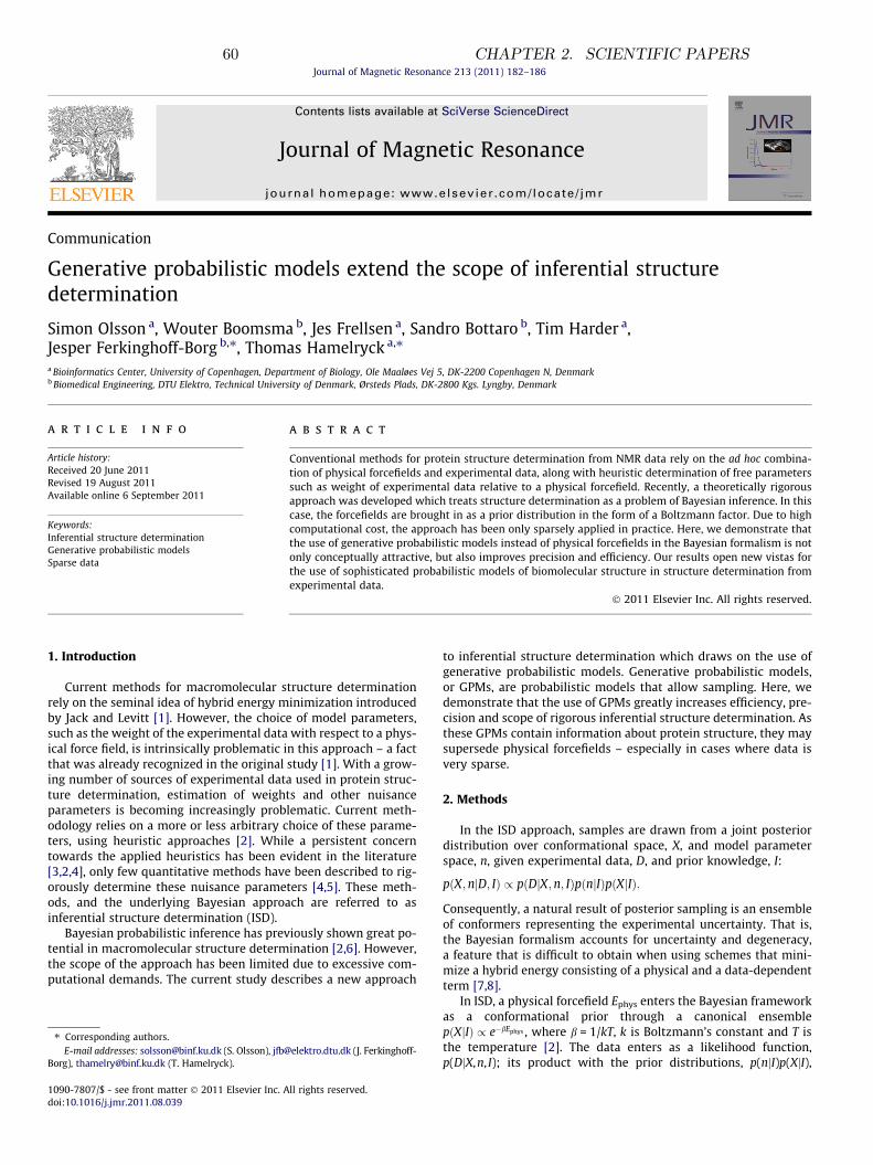
Communication

Generative probabilistic models extend the scope of inferential structuredetermination

Simon Olsson a, Wouter Boomsma b, Jes Frellsen a, Sandro Bottaro b, Tim Harder a,Jesper Ferkinghoff-Borg b,⇑, Thomas Hamelryck a,⇑a Bioinformatics Center, University of Copenhagen, Department of Biology, Ole Maaløes Vej 5, DK-2200 Copenhagen N, Denmarkb Biomedical Engineering, DTU Elektro, Technical University of Denmark, Ørsteds Plads, DK-2800 Kgs. Lyngby, Denmark

a r t i c l e i n f o

Article history:Received 20 June 2011Revised 19 August 2011Available online 6 September 2011

Keywords:Inferential structure determinationGenerative probabilistic modelsSparse data

a b s t r a c t

Conventional methods for protein structure determination from NMR data rely on the ad hoc combina-tion of physical forcefields and experimental data, along with heuristic determination of free parameterssuch as weight of experimental data relative to a physical forcefield. Recently, a theoretically rigorousapproach was developed which treats structure determination as a problem of Bayesian inference. In thiscase, the forcefields are brought in as a prior distribution in the form of a Boltzmann factor. Due to highcomputational cost, the approach has been only sparsely applied in practice. Here, we demonstrate thatthe use of generative probabilistic models instead of physical forcefields in the Bayesian formalism is notonly conceptually attractive, but also improves precision and efficiency. Our results open new vistas forthe use of sophisticated probabilistic models of biomolecular structure in structure determination fromexperimental data.

� 2011 Elsevier Inc. All rights reserved.

1. Introduction

Current methods for macromolecular structure determinationrely on the seminal idea of hybrid energy minimization introducedby Jack and Levitt [1]. However, the choice of model parameters,such as the weight of the experimental data with respect to a phys-ical force field, is intrinsically problematic in this approach – a factthat was already recognized in the original study [1]. With a grow-ing number of sources of experimental data used in protein struc-ture determination, estimation of weights and other nuisanceparameters is becoming increasingly problematic. Current meth-odology relies on a more or less arbitrary choice of these parame-ters, using heuristic approaches [2]. While a persistent concerntowards the applied heuristics has been evident in the literature[3,2,4], only few quantitative methods have been described to rig-orously determine these nuisance parameters [4,5]. These meth-ods, and the underlying Bayesian approach are referred to asinferential structure determination (ISD).

Bayesian probabilistic inference has previously shown great po-tential in macromolecular structure determination [2,6]. However,the scope of the approach has been limited due to excessive com-putational demands. The current study describes a new approach

to inferential structure determination which draws on the use ofgenerative probabilistic models. Generative probabilistic models,or GPMs, are probabilistic models that allow sampling. Here, wedemonstrate that the use of GPMs greatly increases efficiency, pre-cision and scope of rigorous inferential structure determination. Asthese GPMs contain information about protein structure, they maysupersede physical forcefields – especially in cases where data isvery sparse.

2. Methods

In the ISD approach, samples are drawn from a joint posteriordistribution over conformational space, X, and model parameterspace, n, given experimental data, D, and prior knowledge, I:

pðX;njD; IÞ / pðDjX;n; IÞpðnjIÞpðXjIÞ:

Consequently, a natural result of posterior sampling is an ensembleof conformers representing the experimental uncertainty. That is,the Bayesian formalism accounts for uncertainty and degeneracy,a feature that is difficult to obtain when using schemes that mini-mize a hybrid energy consisting of a physical and a data-dependentterm [7,8].

In ISD, a physical forcefield Ephys enters the Bayesian frameworkas a conformational prior through a canonical ensemblepðXjIÞ / e�bEphys , where b = 1/kT, k is Boltzmann’s constant and T isthe temperature [2]. The data enters as a likelihood function,p(DjX,n, I); its product with the prior distributions, p(njI)p(XjI),

1090-7807/$ - see front matter � 2011 Elsevier Inc. All rights reserved.doi:10.1016/j.jmr.2011.08.039

⇑ Corresponding authors.E-mail addresses: [email protected] (S. Olsson), [email protected] (J. Ferkinghoff-

Borg), [email protected] (T. Hamelryck).

Journal of Magnetic Resonance 213 (2011) 182–186

Contents lists available at SciVerse ScienceDirect

Journal of Magnetic Resonance

journal homepage: www.elsevier .com/locate / jmr

60 CHAPTER 2. SCIENTIFIC PAPERS

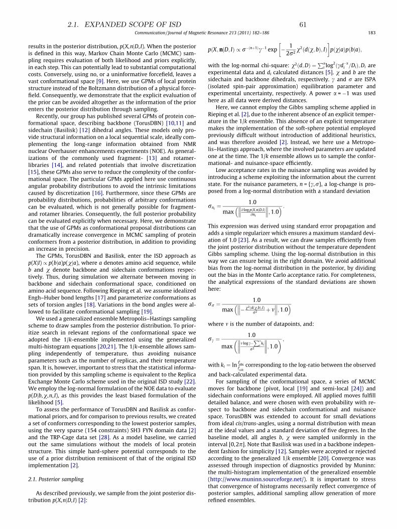
results in the posterior distribution, p(X,njD, I). When the posterioris defined in this way, Markov Chain Monte Carlo (MCMC) sam-pling requires evaluation of both likelihood and priors explicitly,in each step. This can potentially lead to substantial computationalcosts. Conversely, using no, or a uninformative forcefield, leaves avast conformational space [9]. Here, we use GPMs of local proteinstructure instead of the Boltzmann distribution of a physical force-field. Consequently, we demonstrate that the explicit evaluation ofthe prior can be avoided altogether as the information of the priorenters the posterior distribution through sampling.

Recently, our group has published several GPMs of protein con-formational space, describing backbone (TorusDBN) [10,11] andsidechain (Basilisk) [12] dihedral angles. These models only pro-vide structural information on a local sequential scale, ideally com-plementing the long-range information obtained from NMRnuclear Overhauser enhancements experiments (NOE). As general-izations of the commonly used fragment- [13] and rotamer-libraries [14], and related potentials that involve discretization[15], these GPMs also serve to reduce the complexity of the confor-mational space. The particular GPMs applied here use continuousangular probability distributions to avoid the intrinsic limitationscaused by discretization [16]. Furthermore, since these GPMs areprobability distributions, probabilities of arbitrary conformationscan be evaluated, which is not generally possible for fragment-and rotamer libraries. Consequently, the full posterior probabilitycan be evaluated explicitly when necessary. Here, we demonstratethat the use of GPMs as conformational proposal distributions candramatically increase convergence in MCMC sampling of proteinconformers from a posterior distribution, in addition to providingan increase in precision.

The GPMs, TorusDBN and Basilisk, enter the ISD approach asp(XjI) / p(bja)p(vja), where a denotes amino acid sequence, whileb and v denote backbone and sidechain conformations respec-tively. Thus, during simulation we alternate between moving inbackbone and sidechain conformational space, conditioned onamino acid sequence. Following Rieping et al. we assume idealizedEngh–Huber bond lengths [17] and parameterize conformations assets of torsion angles [18]. Variations in the bond angles were al-lowed to facilitate conformational sampling [19].

We used a generalized ensemble Metropolis–Hastings samplingscheme to draw samples from the posterior distribution. To prior-itize search in relevant regions of the conformational space weadopted the 1/k-ensemble implemented using the generalizedmulti-histogram equations [20,21]. The 1/k-ensemble allows sam-pling independently of temperature, thus avoiding nuisanceparameters such as the number of replicas, and their temperaturespan. It is, however, important to stress that the statistical informa-tion provided by this sampling scheme is equivalent to the ReplicaExchange Monte Carlo scheme used in the original ISD study [22].We employ the log-normal formulation of the NOE data to evaluatep(Djb,v,n, I), as this provides the least biased formulation of thelikelihood [5].

To assess the performance of TorusDBN and Basilisk as confor-mational priors, and for comparison to previous results, we createda set of conformers corresponding to the lowest posterior samples,using the very sparse (154 constraints) SH3 FYN domain data [2]and the TRP-Cage data set [28]. As a model baseline, we carriedout the same simulations without the models of local proteinstructure. This simple hard-sphere potential corresponds to theuse of a prior distribution reminiscent of that of the original ISDimplementation [2].

2.1. Posterior sampling

As described previously, we sample from the joint posterior dis-tribution p(X,njD, I) [2]:

pðX;njD; IÞ / r�ðnþ1Þc�1 exp � 12r2 v2ðdðv; bÞ; IÞ

� �pðvjaÞpðbjaÞ;

with the log-normal chi-square: v2ðd;DÞ ¼Pn

i log2ðcd�ai =DiÞ;Di are

experimental data and di calculated distances [5]. v and b are thesidechain and backbone dihedrals, respectively. c and r are ISPA(isolated spin-pair approximation) equilibration parameter andexperimental uncertainty, respectively. A power a = �1 was usedhere as all data were derived distances.

Here, we cannot employ the Gibbs sampling scheme applied inRieping et al. [2], due to the inherent absence of an explicit temper-ature in the 1/k ensemble. This absence of an explicit temperaturemakes the implementation of the soft-sphere potential employedpreviously difficult without introduction of additional heuristics,and was therefore avoided [2]. Instead, we here use a Metropo-lis–Hastings approach, where the involved parameters are updatedone at the time. The 1/k ensemble allows us to sample the confor-mational- and nuisance-space efficiently.

Low acceptance rates in the nuisance sampling was avoided byintroducing a scheme exploiting the information about the currentstate. For the nuisance parameters, n = {c,r}, a log-change is pro-posed from a log-normal distribution with a standard deviation

rni¼ 1:0

max @ log pðX;njD;IÞ@ni

�� ;1:0� � :

This expression was derived using standard error propagation andadds a simple regularizer which ensures a maximum standard devi-ation of 1.0 [23]. As a result, we can draw samples efficiently fromthe joint posterior distribution without the temperature dependentGibbs sampling scheme. Using the log-normal distribution in thisway we can ensure being in the right domain. We avoid additionalbias from the log-normal distribution in the posterior, by dividingout the bias in the Monte Carlo acceptance ratio. For completeness,the analytical expressions of the standard deviations are shownhere:

rr ¼1:0

max � v2ðdðv;bÞ;IÞr2 þ m

�� ;1:0� �

where m is the number of datapoints, and:

rc ¼1:0

maxm log c�

Pmi

ki

r2

��;1:0

� � ;

with ki ¼ ln Iiobs

Iicalc

corresponding to the log-ratio between the observed

and back-calculated experimental data.For sampling of the conformational space, a series of MCMC

moves for backbone (pivot, local [19] and semi-local [24]) andsidechain conformations were employed. All applied moves fulfilldetailed balance, and were chosen with even probability with re-spect to backbone and sidechain conformational and nuisancespace. TorusDBN was extended to account for small deviationsfrom ideal cis/trans-angles, using a normal distribution with meanat the ideal values and a standard deviation of five degrees. In thebaseline model, all angles b, v were sampled uniformly in theinterval [0,2p]. Note that Basilisk was used in a backbone indepen-dent fashion for simplicity [12]. Samples were accepted or rejectedaccording to the generalized 1/k ensemble [20]. Convergence wasassessed through inspection of diagnostics provided by Muninn:the multi-histogram implementation of the generalized ensemble(http://www.muninn.sourceforge.net/). It is important to stressthat convergence of histograms necessarily reflect convergence ofposterior samples, additional sampling allow generation of morerefined ensembles.

Communication / Journal of Magnetic Resonance 213 (2011) 182–186 183

2.1. EXPANDED SCOPE OF ISD 61

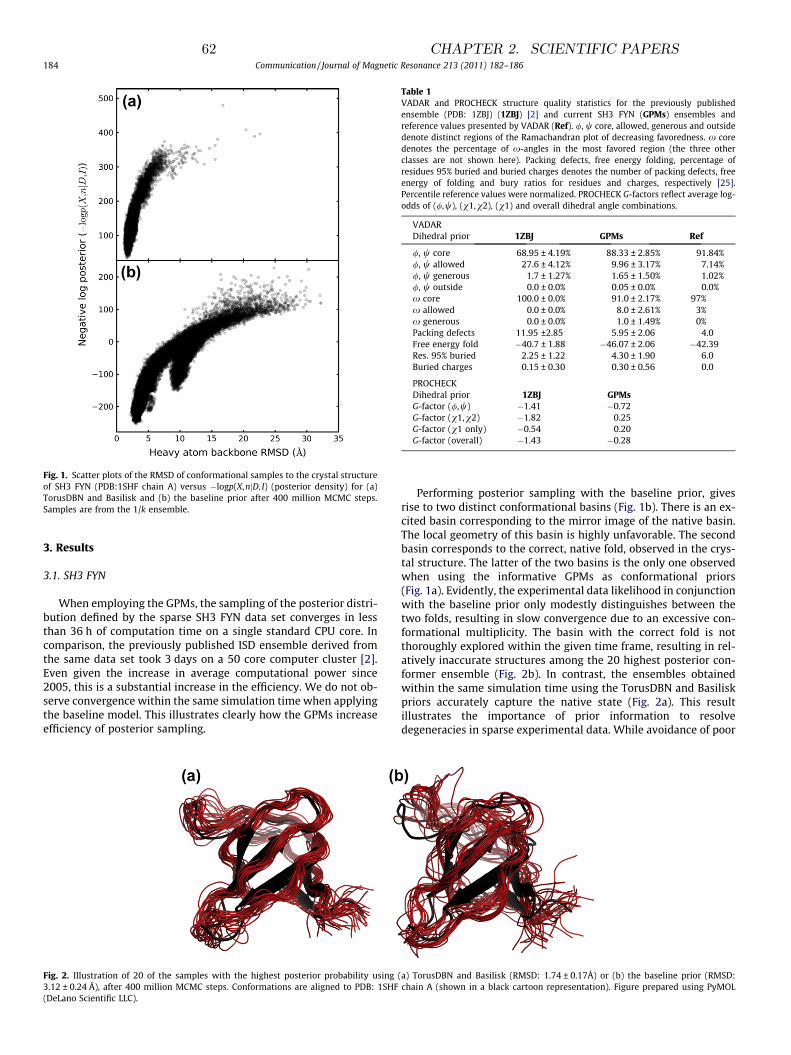
3. Results

3.1. SH3 FYN

When employing the GPMs, the sampling of the posterior distri-bution defined by the sparse SH3 FYN data set converges in lessthan 36 h of computation time on a single standard CPU core. Incomparison, the previously published ISD ensemble derived fromthe same data set took 3 days on a 50 core computer cluster [2].Even given the increase in average computational power since2005, this is a substantial increase in the efficiency. We do not ob-serve convergence within the same simulation time when applyingthe baseline model. This illustrates clearly how the GPMs increaseefficiency of posterior sampling.

Performing posterior sampling with the baseline prior, givesrise to two distinct conformational basins (Fig. 1b). There is an ex-cited basin corresponding to the mirror image of the native basin.The local geometry of this basin is highly unfavorable. The secondbasin corresponds to the correct, native fold, observed in the crys-tal structure. The latter of the two basins is the only one observedwhen using the informative GPMs as conformational priors(Fig. 1a). Evidently, the experimental data likelihood in conjunctionwith the baseline prior only modestly distinguishes between thetwo folds, resulting in slow convergence due to an excessive con-formational multiplicity. The basin with the correct fold is notthoroughly explored within the given time frame, resulting in rel-atively inaccurate structures among the 20 highest posterior con-former ensemble (Fig. 2b). In contrast, the ensembles obtainedwithin the same simulation time using the TorusDBN and Basiliskpriors accurately capture the native state (Fig. 2a). This resultillustrates the importance of prior information to resolvedegeneracies in sparse experimental data. While avoidance of poor

Fig. 1. Scatter plots of the RMSD of conformational samples to the crystal structureof SH3 FYN (PDB:1SHF chain A) versus �logp(X,njD, I) (posterior density) for (a)TorusDBN and Basilisk and (b) the baseline prior after 400 million MCMC steps.Samples are from the 1/k ensemble.

Fig. 2. Illustration of 20 of the samples with the highest posterior probability using (a) TorusDBN and Basilisk (RMSD: 1.74 ± 0.17Å) or (b) the baseline prior (RMSD:3.12 ± 0.24 Å), after 400 million MCMC steps. Conformations are aligned to PDB: 1SHF chain A (shown in a black cartoon representation). Figure prepared using PyMOL(DeLano Scientific LLC).

Table 1VADAR and PROCHECK structure quality statistics for the previously publishedensemble (PDB: 1ZBJ) (1ZBJ) [2] and current SH3 FYN (GPMs) ensembles andreference values presented by VADAR (Ref). /, w core, allowed, generous and outsidedenote distinct regions of the Ramachandran plot of decreasing favoredness. x coredenotes the percentage of x-angles in the most favored region (the three otherclasses are not shown here). Packing defects, free energy folding, percentage ofresidues 95% buried and buried charges denotes the number of packing defects, freeenergy of folding and bury ratios for residues and charges, respectively [25].Percentile reference values were normalized. PROCHECK G-factors reflect average log-odds of (/,w), (v1,v2), (v1) and overall dihedral angle combinations.

VADARDihedral prior 1ZBJ GPMs Ref

/, w core 68.95 ± 4.19% 88.33 ± 2.85% 91.84%/, w allowed 27.6 ± 4.12% 9.96 ± 3.17% 7.14%/, w generous 1.7 ± 1.27% 1.65 ± 1.50% 1.02%/, w outside 0.0 ± 0.0% 0.05 ± 0.0% 0.0%x core 100.0 ± 0.0% 91.0 ± 2.17% 97%x allowed 0.0 ± 0.0% 8.0 ± 2.61% 3%x generous 0.0 ± 0.0% 1.0 ± 1.49% 0%Packing defects 11.95 ±2.85 5.95 ± 2.06 4.0Free energy fold �40.7 ± 1.88 �46.07 ± 2.06 �42.39Res. 95% buried 2.25 ± 1.22 4.30 ± 1.90 6.0Buried charges 0.15 ± 0.30 0.30 ± 0.56 0.0

PROCHECKDihedral prior 1ZBJ GPMsG-factor (/,w) �1.41 �0.72G-factor (v1,v2) �1.82 0.25G-factor (v1 only) �0.54 0.20G-factor (overall) �1.43 �0.28

184 Communication / Journal of Magnetic Resonance 213 (2011) 182–186


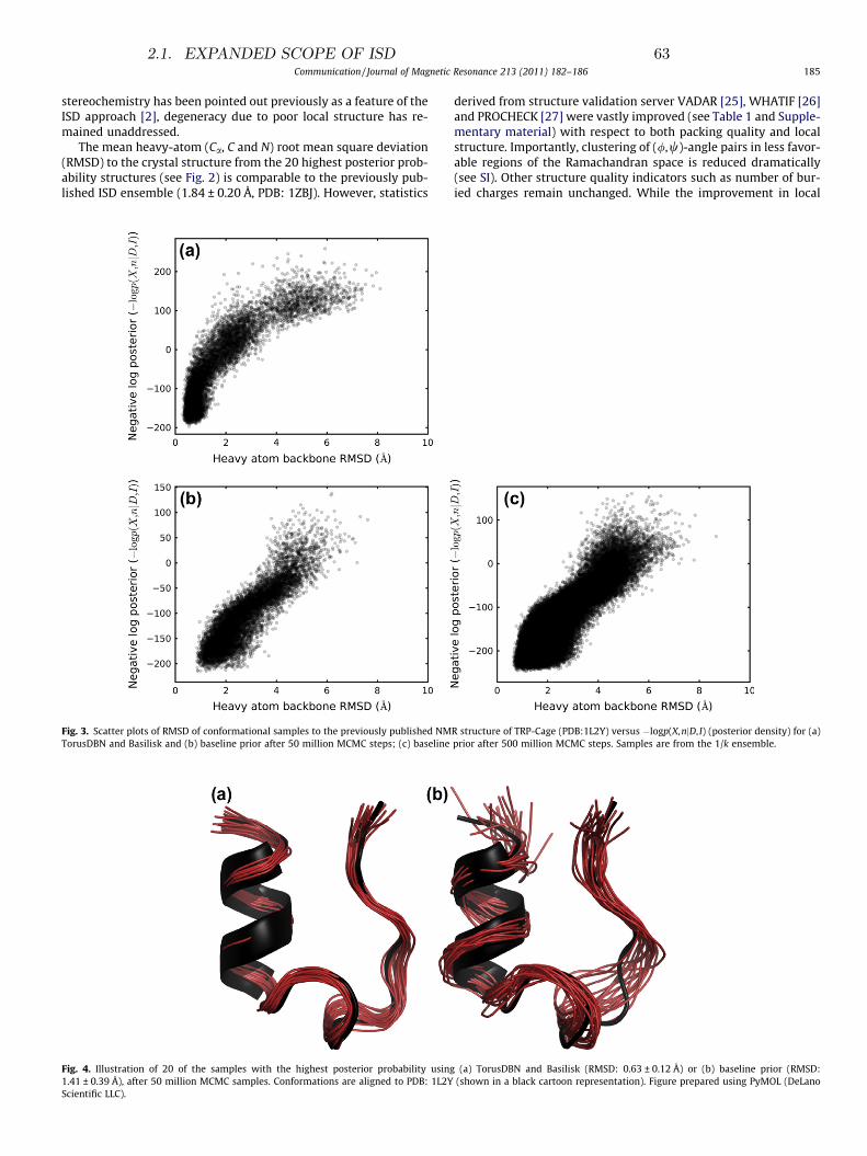
stereochemistry has been pointed out previously as a feature of theISD approach [2], degeneracy due to poor local structure has re-mained unaddressed.

The mean heavy-atom (Ca, C and N) root mean square deviation(RMSD) to the crystal structure from the 20 highest posterior prob-ability structures (see Fig. 2) is comparable to the previously pub-lished ISD ensemble (1.84 ± 0.20 Å, PDB: 1ZBJ). However, statistics

derived from structure validation server VADAR [25], WHATIF [26]and PROCHECK [27] were vastly improved (see Table 1 and Supple-mentary material) with respect to both packing quality and localstructure. Importantly, clustering of (/,w)-angle pairs in less favor-able regions of the Ramachandran space is reduced dramatically(see SI). Other structure quality indicators such as number of bur-ied charges remain unchanged. While the improvement in local

Fig. 3. Scatter plots of RMSD of conformational samples to the previously published NMR structure of TRP-Cage (PDB:1L2Y) versus �logp(X,njD, I) (posterior density) for (a)TorusDBN and Basilisk and (b) baseline prior after 50 million MCMC steps; (c) baseline prior after 500 million MCMC steps. Samples are from the 1/k ensemble.

Fig. 4. Illustration of 20 of the samples with the highest posterior probability using (a) TorusDBN and Basilisk (RMSD: 0.63 ± 0.12 Å) or (b) baseline prior (RMSD:1.41 ± 0.39 Å), after 50 million MCMC samples. Conformations are aligned to PDB: 1L2Y (shown in a black cartoon representation). Figure prepared using PyMOL (DeLanoScientific LLC).

Communication / Journal of Magnetic Resonance 213 (2011) 182–186 185


structure is an expected consequence of the information containedin TorusDBN and Basilisk, non-local structure quality parameterssuch as packing defects hint increase in accuracy. The nuisanceparameters r, c were estimated to be 0.11 ± 0.01 and 1.00 ± 0.01,respectively. These values deviate somewhat from the estimatesobtained previously. The discrepancy may be linked to a differentconformational prior distribution [2].

3.2. TRP-cage

In addition to increasing efficiency and precision, GPMs can ac-count for the information derived from ambiguous NOE con-straints. We demonstrate this point on the TRP-cage data set[28]. Of the reported 169 restraints, 37 involve pseudo atoms,which strictly speaking yields them ambiguous. In these particularcalculations, the restraints were therefore not included. The result-ing set of unambiguous NOE restraints are insufficiently informa-tive to distinguish native-like structures from conformers withan RMSD of up to 3 Å from the previously published NMR struc-ture. However, when we use the GPMs as structural priors, we ob-tain an ensemble of high resemblance with the previouslypublished structure.

The simulations of TRP-cage were performed identically tothose of SH3 FYN using 50 million MCMC steps. Both simulationscomplete within a few hours (see Fig. 3a and b). The pattern ob-served for SH3 FYN emerges again: when using GPMs convergencewas reached within the simulation time, whereas convergence wasnot reached using the baseline model. Extending the simulationtime with the baseline model to 500 million MCMC steps resultsin convergence (Fig. 3c). However, the resulting 20 highest poster-ior ensemble is of significantly lower quality (RMSD: 1.24 ± 0.39 Å)than the ensemble obtained using the GPMs running for 50 millionMCMC steps, Fig. 4a. With these results we again demonstrate howefficiency is gained when employing GPMs in the ISD approach. Inaddition the results illustrate, how the unambiguous constraints[28] can be complemented by the local information contained inthe GPMs.

4. Conclusions

In both examples presented here, the difference in accuracy ofthe selected ensembles is modest, with mean RMSD differencesof at most 1 Å. However, the highest probability (or lowest energy)criterion for selection of conformation for these ensembles maynot only underestimate the spread of the ensemble [29,30], butalso ignore severe degeneracies (see Figs. 1 and 3). This points tothe importance of using appropriate prior information when ana-lyzing sparse data and suggests extra caution be taken whenselecting these ensembles.

This communication describes how generative probabilisticmodels can be applied to significantly increase efficiency and pre-cision of inferential structure determination. As a natural exten-sion, we propose the development of more specialized GPMs,drawing on additional prior information such as protein familymembership or chemical shifts. Such models would presumablyresolve degeneracies to an even greater extent, further increasingthe scope, efficiency and precision of the inferential structuredetermination approach.

Acknowledgments

We thank F.M. Poulsen, K. Lindorff-Larsen and J.H. Jensen forcritically reading the manuscript. T. Harder is funded by the DanishCouncil for Strategic Research (NaBiIT, 2106-06-009). W. Boomsmais funded by the Danish Council for Independent Research (FNU,

272-08-0315). J. Frellsen and S. Olsson are funded by the DanishCouncil for Independent Research (FTP, 09-066546). S. Bottaroacknowledge funding from Radiometer, DTU.Elektro.

Appendix A. Supplementary material

Supplementary data associated with this article can be found, inthe online version, at doi:10.1016/j.jmr.2011.08.039.

References

[1] A. Jack, M. Levitt, Refinement of large structures by simultaneous minimizationof energy and R factor, Acta Crystallogr. A 34 (1978) 931–935.

[2] W. Rieping, M. Habeck, M. Nilges, Inferential structure determination, Science309 (2005) 303–306.

[3] M. Williamson, C. Craven, Automated protein structure calculation from NMRdata, J. Biomol. NMR 43 (2009) 131–143. doi:10.1007/s10858-008-9295-6.

[4] M. Habeck, W. Rieping, M. Nilges, Weighting of experimental evidence inmacromolecular structure determination, Proc. Natl. Acad. Sci. USA 103 (2006)1756–1761.

[5] W. Rieping, M. Habeck, M. Nilges, Modeling errors in NOE data with a log-normal distribution improves the quality of NMR structures, J. Am. Chem. Soc.127 (2005) 16026–16027.

[6] C.K. Fisher, A. Huang, C.M. Stultz, Modeling intrinsically disordered proteinswith bayesian statistics, J. Am. Chem. Soc. 132 (2010) 14919–14927.

[7] C. Schwieters, J. Kuszewski, N. Tjandra, G. Clore, The Xplor-NIH NMR molecularstructure determination package, J. Magn. Reson. 160 (2003) 66–74.

[8] W. Rieping, M. Habeck, B. Bardiaux, A. Bernard, T. Malliavin, M. Nilges, Aria2:automated NOE assignment and data integration in NMR structure calculation,Bioinformatics 23 (2007) 381–382.

[9] M. Habeck, Statistical mechanics analysis of sparse data, J. Struct. Biol. (2010).[10] T. Hamelryck, J.T. Kent, A. Krogh, Sampling realistic protein conformations

using local structural bias, PLoS Comput. Biol. 2 (2006) e131.[11] W. Boomsma, K.V. Mardia, C.C. Taylor, J. Ferkinghoff-Borg, A. Krogh, T.

Hamelryck, A generative, probabilistic model of local protein structure, Proc.Natl. Acad. Sci. USA 105 (2008) 8932–8937.

[12] T. Harder, W. Boomsma, M. Paluszewski, J. Frellsen, K.E. Johansson, T.Hamelryck, Beyond rotamers: a generative, probabilistic model of sidechains in proteins, BMC Bioinf. 11 (2010) 306.

[13] K.T. Simons, C. Kooperberg, E. Huang, D. Baker, Assembly of protein tertiarystructures from fragments with similar local sequences using simulatedannealing and Bayesian scoring functions, J. Mol. Biol. 268 (1997) 209–225.

[14] S.C. Lovell, J.M. Word, J.S. Richardson, D.C. Richardson, The penultimaterotamer library, Proteins 40 (2000) 389–408.

[15] J. Kuszewski, A.M. Gronenborn, G.M. Clore, Improving the quality of NMR andcrystallographic protein structures by means of a conformational databasepotential derived from structure databases, Prot. Sci. 5 (1996) 1067–1080.

[16] G.L. Butterfoss, B. Kuhlman, Computer-based design of novel proteinstructures, Annu. Rev. Biophys. Biomol. Struct. 35 (2006) 49–65.

[17] R.A. Engh, R. Huber, Accurate bond and angle parameters for X-ray proteinstructure refinement, Acta Cryst. A47 (1991) 392–400.

[18] L.M. Rice, A.T. Brünger, Torsion angle dynamics: reduced variableconformational sampling enhances crystallographic structure refinement,Proteins 19 (1994) 277–290.

[19] S. Bottaro, W. Boomsma, K.E. Johansson, C. Andreetta, T. Hamelryck, J.Ferkinghoff-Borg, Realizing the potential of Monte Carlo: subtle kinetics indense protein systems, unpublished results.

[20] B. Hesselbo, R.B. Stinchcombe, Monte Carlo simulation and global optimizationwithout parameters, Phys. Rev. Lett. 74 (1995) 2151–2155.

[21] J. Ferkinghoff-Borg, Optimized Monte Carlo analysis for generalizedensembles, Eur. Phys. J. B 29 (2002) 481–484.

[22] M. Habeck, M. Nilges, W. Rieping, Replica-exchange Monte Carlo scheme forBayesian data analysis, Phys. Rev. Lett. 94 (2005) 018105-1–018105-4.

[23] S. Meyer, Data Analysis for Scientists and Engineers, Wiley, 1975.[24] G. Favrin, A. Irbäck, F. Sjunnesson, Monte Carlo update for chain molecules:

biased Gaussian steps in torsional space, J. Chem. Phys. 114 (2001) 8154–8158.[25] L. Willard, A. Ranjan, H. Zhang, H. Monzavi, R.F. Boyko, B.D. Sykes, D.S. Wishart,

Vadar: a web server for quantitative evaluation of protein structure quality,Nucleic Acids Res. 31 (2003) 3316–3319.

[26] G. Vriend, WHAT IF: a molecular modeling and drug design program, J. Mol.Graph. 8 (1990). 52–56, 29.

[27] R.A. Laskowski, M.W. MacArthur, D.S. Moss, J.M. Thornton, Procheck: aprogram to check the stereochemical quality of protein structures, J. Appl.Crystallogr. 26 (1993) 283–291.

[28] J.W. Neidigh, R.M. Fesinmeyer, N.H. Andersen, Designing a 20-residue protein,Nat. Struct. Biol. 9 (2002) 425–430.

[29] D. Zhao, O. Jardetzky, An assessment of the precision and accuracy of proteinstructures determined by NMR: dependence on distance errors, J. Mol. Biol.239 (1994) 601–607.

[30] C.A. Spronk, S.B. Nabuurs, A.M. Bonvin, E. Krieger, G.W. Vuister, G. Vriend, Theprecision of NMR structure ensembles revisited, J. Biomol. NMR 25 (2003)225–234. 10.1023/A:1022819716110.

186 Communication / Journal of Magnetic Resonance 213 (2011) 182–186


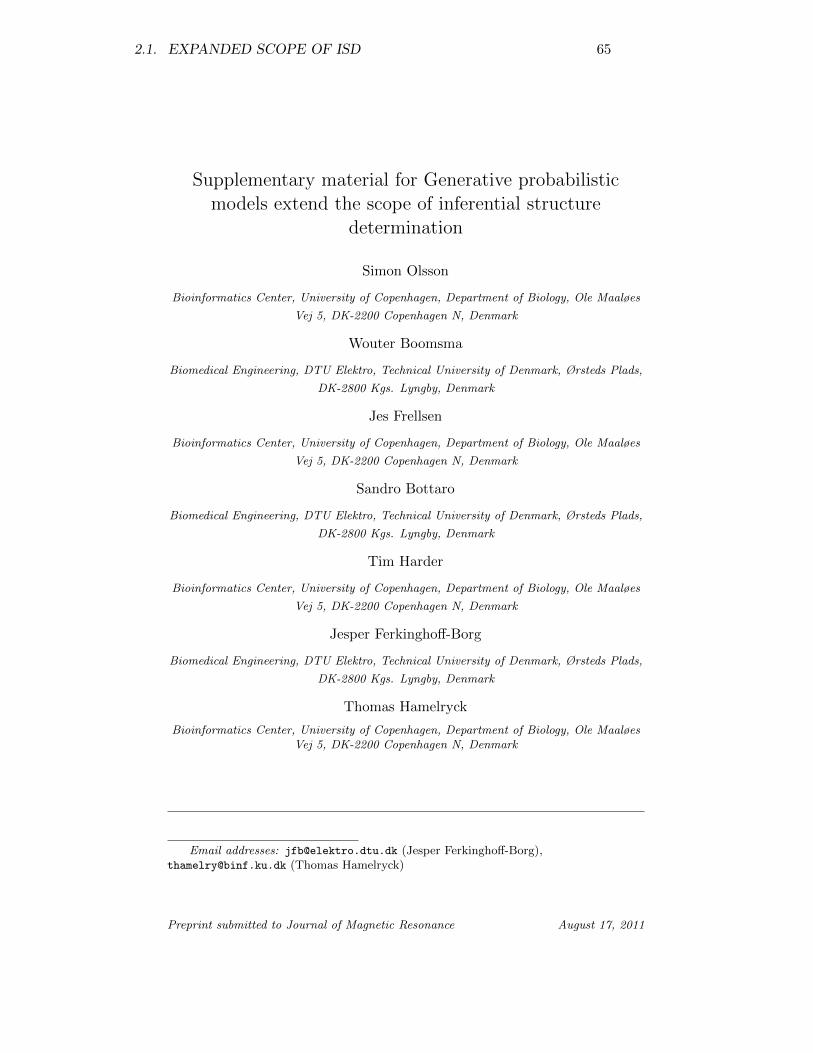
Supplementary material for Generative probabilisticmodels extend the scope of inferential structure

determination

Simon Olsson

Bioinformatics Center, University of Copenhagen, Department of Biology, Ole Maaløes

Vej 5, DK-2200 Copenhagen N, Denmark

Wouter Boomsma

Biomedical Engineering, DTU Elektro, Technical University of Denmark, Ørsteds Plads,

DK-2800 Kgs. Lyngby, Denmark

Jes Frellsen



Sandro Bottaro



Tim Harder



Jesper Ferkinghoff-Borg



Thomas Hamelryck

Bioinformatics Center, University of Copenhagen, Department of Biology, Ole MaaløesVej 5, DK-2200 Copenhagen N, Denmark

Email addresses: [email protected] (Jesper Ferkinghoff-Borg),[email protected] (Thomas Hamelryck)

Preprint submitted to Journal of Magnetic Resonance August 17, 2011


1. Posterior sampling details

In addition to bond lengths, ring planarities are kept fixed. These are

reasonable approximations at room temperature. Furthermore, to avoid

sterical overlap we impose a hard sphere volume exclusion potential with

conservative distance cutoffs at 1.3A for H − H pairs, 1.65A for N − O

pairs and 1.5A for any other pair of atoms. No clashing conformers were

considered. All calculations were carried out using the Phaistos framework

(http://www.phaistos.org) [1]. Support for NOE constraints will be added

to the Phaistos package in the near future. The conformers for the final

ensembles were selected by reweighing the samples from the 1/k ensem-

ble according to the posterior distribution and selecting the 20 most likely

conformers.

2. Quantitative Assessment of Structure Quality

During sampling the conformational priors, TorusDBN and Basilisk are

generally not evaluated explicitly, e.g. P (X|I) is only used as a proposal

distribution of the conformational space, without accounting for sampling

bias in the Monte-Carlo acceptance ratio. Thus, the likelihood function

p(D|X, I) is the only explicitly evaluated term in each evaluation step of

the simulation. Posterior probabilities are determined by multiplying prior

probabilities evaluated from TorusDBN and Basilisk with the likelihood of

samples obtained from the simulation. All results were based on samples

saved with a regular interval of 10000 MCMC steps during simulation, for

which the full posterior was used.

2


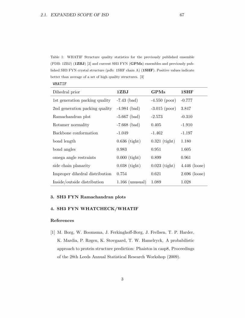
Table 1: WHATIF Structure quality statistics for the previously published ensemble

(PDB: 1ZBJ) (1ZBJ) [2] and current SH3 FYN (GPMs) ensembles and previously pub-

lished SH3 FYN crystal structure (pdb: 1SHF chain A) (1SHF). Positive values indicate

better than average of a set of high quality structures. [3]

WHATIF

Dihedral prior 1ZBJ GPMs 1SHF

1st generation packing quality -7.43 (bad) -4.550 (poor) -0.777

2nd generation packing quality -4.984 (bad) -3.015 (poor) 3.847

Ramachandran plot -5.667 (bad) -2.573 -0.310

Rotamer normality -7.668 (bad) 0.405 -1.910

Backbone conformation -1.049 -1.462 -1.197

bond length 0.636 (tight) 0.321 (tight) 1.180

bond angles 0.983 0.951 1.605

omega angle restraints 0.000 (tight) 0.899 0.961

side chain planarity 0.038 (tight) 0.023 (tight) 4.446 (loose)

Improper dihedral distribution 0.754 0.621 2.696 (loose)

Inside/outside distribution 1.166 (unusual) 1.089 1.028

3. SH3 FYN Ramachandran plots

4. SH3 FYN WHATCHECK/WHATIF

References

[1] M. Borg, W. Boomsma, J. Ferkinghoff-Borg, J. Frellsen, T. P. Harder,

K. Mardia, P. Røgen, K. Stovgaard, T. W. Hamelryck, A probabilistic

approach to protein structure prediction: Phaistos in casp8, Proceedings

of the 28th Leeds Annual Statistical Research Workshop (2009).

3


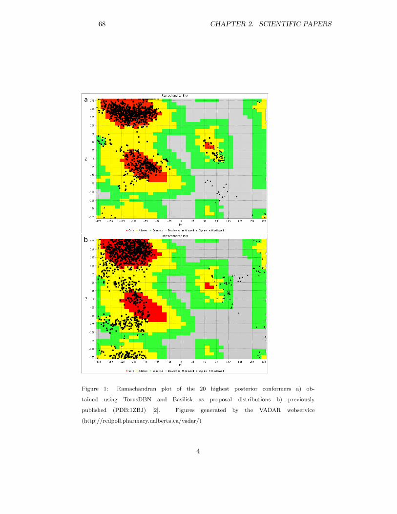
Figure 1: Ramachandran plot of the 20 highest posterior conformers a) ob-

tained using TorusDBN and Basilisk as proposal distributions b) previously

published (PDB:1ZBJ) [2]. Figures generated by the VADAR webservice

(http://redpoll.pharmacy.ualberta.ca/vadar/)

4


[2] W. Rieping, M. Habeck, M. Nilges, Inferential structure determination.,

Science 309 (2005) 303–306.

[3] G. Vriend, WHAT IF: a molecular modeling and drug design program.,

J. Mol. Graph. 8 (1990) 52–6, 29.

5



2.2 Inferential determination of protein structural ensem-bles from sparse, averaged data.

The determination of ensembles of structures which gives rise to a partic-ular spatially and temporally averaged experimental signal continues to bean important problem. We here approach the problem from a probabilis-tic perspective, and obtain a hierarchical model which contains previouslyproposed methods as intuitive limits.

To illustrate the model is tractable, we apply the model to two datasetof simulated nuclear Overhauser enhancements. We find that we are ableto accurately reconstruct the probability distributions of the geometricalfeatures reflected in the data.This is a first author paper and I was involved in all aspects of the workcarried out. Submitted for publication.

1

Inference of protein structure ensembles from sparse, averageddata.Simon Olsson1∗, Jes Frellsen1, Wouter Boomsma2, Kanti V. Mardia3 and Thomas Hamelryck1∗

1 Bioinformatics Centre, Department of Biology, Faculty of Science, University ofCopenhagen, Copenhagen, Denmark2 Structural Biology and NMR Laboratory, Department of Biology, Faculty ofScience, University of Copenhagen, Copenhagen, Denmark3 Department of Statistics, School of Mathematics, University of Leeds, Leeds,United Kingdom.∗ E-mail: Corresponding [email protected], [email protected]

Abstract

We present a general principle to infer protein structure ensembles from spatially and temporallyaveraged data obtained in biophysical experiments. The central idea is to compute the Kullback-Leibler optimal modification of a given prior distribution τ(x) with respect to the experimentaldata and its uncertainty. This principle generalizes the successful inferential structure determi-nation method and recently proposed maximum entropy methods. Tractability of the protocolis demonstrated through the analysis of simulated nuclear magnetic resonance spectroscopy dataof a small peptide.

Introduction

The rigorous analysis of experimental data probing the structure of biological macromoleculesforms the foundation of many biophysical studies [1]. The sources of experimental data includenuclear magnetic resonance spectroscopy spectroscopy (NMR) and small-angle X-ray- and neu-tron scattering. This article addresses several issues which often make inference of biomolecularstructure from such data particularly challenging. First, in these experiments, the time-scaleof acquisition typically exceeds that of molecular fluctuations. Second, the samples studied areoften near molar concentrations. Third, data is frequently incomplete, or even sparse, and sub-ject to experimental noise. Consequently, data obtained from such techniques yield incomplete,noisy, spatially and temporally averaged information on the Boltzmann ensemble of the ob-served system. Thus, such data are ideally analyzed through models that take these propertiesinto account. While this fact has long been recognized, the analysis of these types of data hasrevolved predominantly around structure determination – that is, fitting a single conformationto fulfill all derived geometrical restraints [2]. Such structure determination methods do notadequately handle sparse, noisy and averaged data. Here, we propose an alternative methodwhich addresses these shortcomings.

Typically, structure determination from experimental data proceeds through hybrid energyminimization [3]. In this method, an energy function Eexp that brings in the experimentaldata is combined with an approximative physical forcefield Ephys. The term Eexp is typicallya straight-forward combination of a forward- and an error-model. A forward-model relates

2.2. INFERENCE OF PROTEIN STRUCTURE ENSEMBLES 71

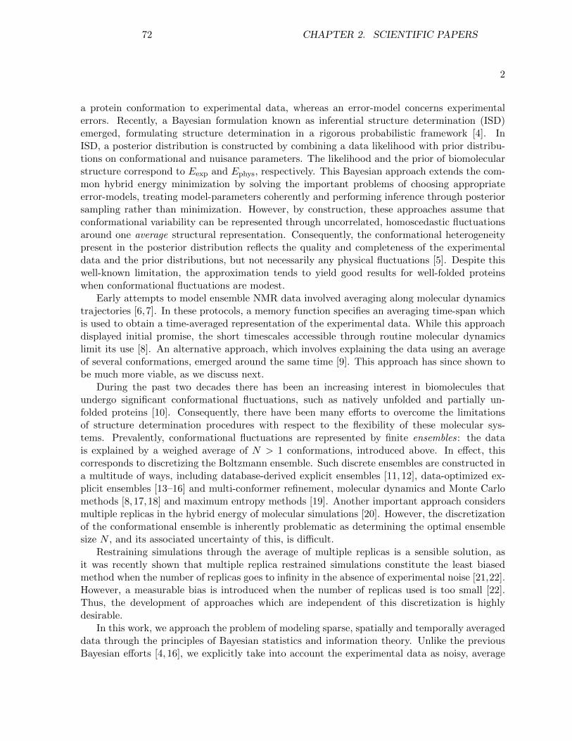
2

a protein conformation to experimental data, whereas an error-model concerns experimentalerrors. Recently, a Bayesian formulation known as inferential structure determination (ISD)emerged, formulating structure determination in a rigorous probabilistic framework [4]. InISD, a posterior distribution is constructed by combining a data likelihood with prior distribu-tions on conformational and nuisance parameters. The likelihood and the prior of biomolecularstructure correspond to Eexp and Ephys, respectively. This Bayesian approach extends the com-mon hybrid energy minimization by solving the important problems of choosing appropriateerror-models, treating model-parameters coherently and performing inference through posteriorsampling rather than minimization. However, by construction, these approaches assume thatconformational variability can be represented through uncorrelated, homoscedastic fluctuationsaround one average structural representation. Consequently, the conformational heterogeneitypresent in the posterior distribution reflects the quality and completeness of the experimentaldata and the prior distributions, but not necessarily any physical fluctuations [5]. Despite thiswell-known limitation, the approximation tends to yield good results for well-folded proteinswhen conformational fluctuations are modest.

Early attempts to model ensemble NMR data involved averaging along molecular dynamicstrajectories [6,7]. In these protocols, a memory function specifies an averaging time-span whichis used to obtain a time-averaged representation of the experimental data. While this approachdisplayed initial promise, the short timescales accessible through routine molecular dynamicslimit its use [8]. An alternative approach, which involves explaining the data using an averageof several conformations, emerged around the same time [9]. This approach has since shown tobe much more viable, as we discuss next.

During the past two decades there has been an increasing interest in biomolecules thatundergo significant conformational fluctuations, such as natively unfolded and partially un-folded proteins [10]. Consequently, there have been many efforts to overcome the limitationsof structure determination procedures with respect to the flexibility of these molecular sys-tems. Prevalently, conformational fluctuations are represented by finite ensembles: the datais explained by a weighed average of N > 1 conformations, introduced above. In effect, thiscorresponds to discretizing the Boltzmann ensemble. Such discrete ensembles are constructed ina multitude of ways, including database-derived explicit ensembles [11, 12], data-optimized ex-plicit ensembles [13–16] and multi-conformer refinement, molecular dynamics and Monte Carlomethods [8,17,18] and maximum entropy methods [19]. Another important approach considersmultiple replicas in the hybrid energy of molecular simulations [20]. However, the discretizationof the conformational ensemble is inherently problematic as determining the optimal ensemblesize N , and its associated uncertainty of this, is difficult.

Restraining simulations through the average of multiple replicas is a sensible solution, asit was recently shown that multiple replica restrained simulations constitute the least biasedmethod when the number of replicas goes to infinity in the absence of experimental noise [21,22].However, a measurable bias is introduced when the number of replicas used is too small [22].Thus, the development of approaches which are independent of this discretization is highlydesirable.

In this work, we approach the problem of modeling sparse, spatially and temporally averageddata through the principles of Bayesian statistics and information theory. Unlike the previousBayesian efforts [4, 16], we explicitly take into account the experimental data as noisy, average


3

quantities of an underlying heterogenous ensemble in continuous space. We derive a generalposterior distribution from first principles which imposes the least necessary bias on our priorknowledge to fulfill the experimental data. Furthermore we illustrate its tractability throughapplying the method to a sparse, synthetic dataset generated from the small peptide GB1 usingthe PROFASI forcefield at high temperature [23].

Results & Discussion

A hierarchical model of spatially and temporally averaged restraints

Ultimately, our aim is to sample from the conditional probability distribution p(x | d), where xdenotes a protein’s conformation and d denotes spatially and temporally averaged, experimentaldata. The variable x represents a positional microstate in atomic detail. Through a forwardmodel f(x) we can calculate a coarse-grained representation, f , of a protein conformation x.That is, our forward model is a mapping, f : R3N → RM , of the N atoms of x to an M <3N -dimensional coarse grained representation, f . Conceptually, f may be interpreted as theinstantaneous ’experimental data’ back-calculated from a positional micro-state, x. However, asd represents an averaged quantity we need to introduce a variable, e, to represent an ensembleaverage of the simulated experimental data f . Consequently, our full posterior distributionbecomes p(x, f , e | d).

We clarify the relation between f , e and d using the example we will present later on. In thecase of nuclear Overhauser enhancement (NOE) data obtained from an NMR experiment [24],the coarse-grained variable f is a vector related to pairwise distances between atoms in a proteinconformation x. In one case, this is simply a vector of these distances. The variable e is anaverage of f vectors from an ensemble of protein conformations. The experimental NOE datad can be interpreted as a noisy observation of the vector of averages, e. In general, there is nosimple relationship between the vector f and the averaged vector e, but a simple probabilisticmodel that relates them can be developed, as we discuss next.

We start by considering the coarse-grained representations of the distribution, f , e andd, without considering the fine-grained representation, x. Following the Bayesian probabilitycalculus, we formulate a posterior distribution:

p(f , e | d) ∝ p(d | f , e)π(f , e)

= p(d | e)π(f , e),(1)

where the first term is the likelihood and the second term is the prior distribution. The equalityis due to the redundancy of f in the evaluation of the likelihood function – d is a noisy observationof e, which does not involve f . The independence assumptions of the model are shown in thecorresponding graphical model in figure 1.

Applying the product rule of probability theory to equation (1), we obtain

p(f , e | d) ∝ p(d | e)πf (f | e)πe(e). (2)

πf (f | e) is the prior distribution of the simulated data f given their averaged value e, and πe(e)is the prior distribution over the simulated ensemble averaged data e.


4

Equation (2) is a probabilistic model of the relationship between noisy, ensemble averageddata, and conformational micro-states in a coarse-gained space. However, to obtain a probabilitydistribution p(x, f , e | d) which features atomic detail, we need to combine (2) with a fine-grainedphysical forcefield or a probability distribution, τ(x). This can be done by using the referenceratio method [25]:

p(x, f , e | d) ∝ p(d | e)πf (f | e)πe(e)

τf (f)τ(x). (3)

τf (f) is called the reference distribution, and is the distribution induced in the coarse-grainedspace by the fine-grained prior, τ(x). The reference distribution arises as a prior on x directlyimplies a prior on f , due to the deterministic relationship between the parameters through theforward model f(·). The reference ratio method yields the Kullback-Leibler optimal modificationof the fine-grained model τ(x) with respect to the coarse-grained information (for proof, seechapter 4 in [26]). Kullback-Leibler optimality is closely linked to the maximum entropy principleof Jaynes [27]. In essence, our approach can be seen as a maximum entropy solution given thenoisy observation of an ensemble average. It should be noted that even if the distribution givenby Equation (2) is unimodal, the posterior given by Equation (3) can still be multimodal dueto the nature of the conformational prior, τ(x).

The relationship to other methods

The model given by Equation (3) may be reduced to the ISD framework [4]

p(x, f | d) ∝ p(d | f)τ(x) (4)

if we choose the Dirac delta function δ(f − e) for πf (f | e)πe(e) and assume that τf (f) isuniform. Choosing the Dirac delta function corresponds to assuming the Boltzmann distributionis infinitely narrow. Hence, our model can be seen as a generalization of ISD. The choice of theuniform distribution for τf (f) corresponds to assuming that τ(x) implies a suitable prior for fas well. This may be inappropriate in some cases (see below).

We also observe that Equation (2) may be reduced to the previously proposed maximumentropy restraining methods [21,22]. This is evident if we consider the case where p(d | e) is thenormal distribution and πf (f | e)πe(e) is a log-linear model (G(·)) with a linear link-function,`(A,b) = Ab. The link function allows us to include the Lagrange multipliers used to relatethe coarse-grained variable f to the mean value f [28]. Thus, G(f | Λ, e) = exp [c+ f`(Λ, e)] ∝exp(fΛe). We have

p(f , e | d) ∝ p(d | e)πf (f | e)πe(e) = N (d | e, σ)G(f | Λ, e) (5)

where Λ is a diagonal matrix of Lagrange multipliers. If we now consider the limit where theexperimental noise vanishes we obtain,

limσ→0N (d | e, σ)G(f | Λ, e) = G(f | Λ,d). (6)

In minus log-space Equation 6 is proportional to minus fΛd. This corresponds to the empiricalterm of the previously reported maximum entropy method in absence of experimental uncer-tainty [21]. We note that this method does not explicitly account for the reference distribution


5

τf (f) when combining the empirical term in the coarse-grained space with a fine-grained priordistribution, τ(x). However, if the prior τf (f) is appropriate then the Lagrange multipliers Λmay provide the necessary means for minor adjustments.

Reconstructing a high temperature ensemble from sparse data and a proba-bilistic prior of local protein structure

To test our model, we use synthetic NOE data, obtained from an ensemble of the GB1 hair-pin simulated at 400K in the Profasi forcefield [23]. The restraints are visualized on a randomconformation of the GB1 hairpin in Figure 2. Historically, NOEs constitute one of the mostimportant sources of semi-quantitative information in NMR structure determination. Underthe isolated spin-pair approximation for rigid molecules, NOEs are related to an interatomicdistance r as NOE ∝ 〈r−6〉 [29]. As an example, we will apply equation (2) to two cases ofaveraged pairwise distance data – these two cases involve the arithmetic mean 〈r〉, and thepower-averaged mean 〈r−6〉, respectively. They represent two different averaging processes thatare common in biophysical data.

We use the log-normal distribution as an appropriate error-model for pairwise distancesderived from NOEs, which is the approach adopted by ISD [30]. The choice is less obvious forthe prior πf (f | e) and depends on the type of experimental data. Here, we use the exponential

distribution with mean β, E(x | β) = e− xβ β−1, since it constitutes the least biasing continuous

distribution on the positive real axis, when no higher order moments are observed [31]. Theprior on f thus becomes: πf (f | e) = πf (f | e,w) = ΠiE(fi | eiwi), where the product runs overall data-points and the scale vector w is a free parameter (discussed below). It follows that

p(x, f , e | d) ∝ N (ln d | ln e,σ)πf (f | e,w)πe(e)

τf (f)τ(x), (7)

where σ is the experimental error, which is fixed and given, and N (·) is the normal distribution.As prior on the ensemble average e we choose πe(e) ∝ e−1. This prior has previously beenshown to provide good results for variables confined to the positive real axis [32].

Equation (7) provides an exact solution to the problem of modeling averaged NOE datasubject to experimental uncertainty. The only parameter to be estimated is the scale vector w,which relates f to e in πf (f | e,w).

In the ideal case, an optimal choice for w results in the desired distribution for f as calculatedfrom the structures x. More precisely, it results in a marginal posterior distribution of Equation(7) for x, such that, when e is fixed, the expectation of f is equal to e. In practice, a satisfactorypoint estimate for w can be obtained in an iterative manner, using an empirical Bayes approach(see Materials and Methods). The parameter w compensates for the approximate nature thereference distribution τf (f), which is difficult to estimate accurately [25]. The introduction ofw provides a simple, yet effective measure to compensate for this.

We use equation (7) to model synthetic pairwise distance restraints in the GB1 hairpin. Forτ(x) we use probabilistic models of the conformational space of the main chain [33] and theside chains [34], as these models recently yielded excellent results when combined with the ISDmethod [35]. As the prior distribution and the likelihood concern local and nonlocal features ofprotein structure, respectively, their information content shows little overlap. More informative


6

priors, for example based on physical energy functions, can be envisaged, but this is beyond thescope of this article.

The prior distribution used in this study concerns protein structure on a local length scale,and thus does not model long range distances accurately. Consequently, as a reaction coordinate,we chose a representative distance f0 between atoms Cα41 and Cα51 – which are separatedfarthest in sequence – to illustrate the long-range properties of the eight different ensemblesconsidered here. Histograms of this pair-wise distance in the different ensembles are shown inFigures 3 and 4. This pair-wise distance is highlighted with yellow color in Figure 2.

The conformational prior and PROFASI, which was used to generate the averaged data,result in different distance distributions (Figure 3). However, if we modify the prior using thereference ratio method as described above, we obtain good fits with the PROFASI distributionfor both linearly and power-averaged data. The ISD ensemble, which does not take the ensemblenature of the data into account, is overly tightly peaked around the (correct) mean.

A similar pattern is observed for the distribution of the gyration radii Rg. The gyrationradii are not used in the estimation of the probability distributions, and can thus be used forcross-validation. The average and standard deviation of the gyration radii of the ensemble usedto generate the data is 9.71 ± 1.5A. The ensembles obtained with our method from the poweraveraged and linearly averaged data resulted in a slightly higher average (10.30 ± 1.8A and10.19 ± 1.6A, respectively), but essentially the correct standard deviation. This is an excellentresult, as a perfect fit is not expected due to the sparse and noisy nature of the data. Again,the ISD ensemble provides an overly narrow distribution (9.88± 0.6A). Finally, sampling fromthe prior distribution alone results in an average radius of gyration of 11.34 ± 1.8A, which isconsiderably too high.

In some cases, the bias introduced by the reference distribution is not critical for obtaininggood results. As it constitutes an additional obstacle in terms of estimation and simulation time,we evaluate its significance on the obtained results. In the power averaged case we achieved thisby chosing the reference distribution τf (f) and the scale vector, w, in equation (7) to be theuniform distribution and the unit vector, respectively. In the linearly averaged case, the scalevector was kept fixed equal to the 1-vector, as τf (f) was assumed to be uniform in the resultspresented above. The results are shown in figure 4. In the case of the power averaged data,with τf (f) uniform and w equal to the 1-vector, severely skews the distribution of the distances(green line in figure 4). When the scale vector w is estimated, while still assuming τf (f) uniform,the fit improves (blue line), but without resulting in a satisfactory distribution. In the linearlyaveraged case, we find that a 1-vector for w provides good fit (red line).

If we again consider the gyration radii as providing complementary views of the ensembles,we find that the power-averaged ensemble with uniform τf (f) and unit scale vector yields aoverly extended ensemble, 11.94± 1.63A. The results in the linearly averaged case compare tothose with an estimated scale-vector, 10.34± 1.69A, presented above.

To summarize, in the power averaged case, both τf (f) and w are required for a satisfactorydistribution. In the case of the linearly averaged data, our results suggest that w and τf (f) maybe approximated by the 1-vector and uniform distribution, respectively. This is particularlyinteresting as it may be a general feature of applying other kinds of linearly averaged data. Thiswill make the use of these types of data for restraining easier.


7

Conclusion

In conclusion, we present a Bayesian principle to infer ensembles of protein structures from noisyexperimental data subject to ensemble and time averaging. The principle is successfully appliedand constitutes a generalization of ISD and previously proposed maximum entropy restrainingapproaches. We successfully apply the method to analyze noisy linearly and power averageddata.

Our approach combines a coarse-grained Bayesian model of the data with a fine-grainedmodel of protein conformational space. The combination is accomplished using reference ratiomethod [25], which corresponds to a maximum entropy solution in the presence of experimentalnoise. The role of the reference distribution τf (f) is considerable. When we assumed τf (f) tobe uniform, we were unable to construct sufficiently accurate distribution of pair-wise distancegeometry, in the case of power-averaged data.

The Bayesian model can in principle be applied to denser datasets and to other data suchas small angle X-ray- or neutron scattering data, or other data derived from NMR experiments.Also, low-resolution data may be combined with more sophisticated physical prior distribu-tions such as those embodied in force fields. The presented method is thus a general andefficient method to obtain physically sound ensemble models of solution and endogenous statesof biomolecules, given appropriate experimental data. Similar models could in principle be usedfor other inference problems in physics, biology or medicine that involve spatially or temporallyaveraged data.

Materials and Methods

Synthetic datasets

A synthetic dataset was created for the GB1 hairpin (Protein data bank identifier: 1LE3; se-quence variant [Y45W, F52W, V54W]). The data were generated by simulating the proteinat 400K with the PROFASI forcefield [23], using Engh-Huber parameters for bond-angles andbond-lengths [36]. The high temperature was used to emulate the effect of a denatured, disor-dered state. A total of 3.5 · 108 steps were performed using the Metropolis-Hastings algorithmin the PHAISTOS Markov chain Monte Carlo framework (http://www.phaistos.org). We useda Monte Carlo move set previously described [35]. Samples were saved in intervals of 5000 steps.These samples were used to form five non-redundant, averaged Cα−Cα distance restraints (seeTabel 1).

To mimic the effect of distance averaging in a dipolar interaction undergoing fast motioncompared to the cross-relaxation but slow motion when compared to molecular tumbling, wecalculated a power averaged variant of the dataset as Ii = 〈r−6i 〉, where ri is an inter-atomicdistance and the angular-brackets denote ensemble averaging [37]. We used an experimentaluncertainty for the power averaged dataset σI of the same relative amplitude as for the average

restraint set σd, by enforcing the signal-to-noise ratio to be constant. Hence, dσd

= IσI⇒ σI = I

d,

as σd = 1, where I and d denote the datapoints corresponding to the largest average distancein the power and linearly averaged datasets, respectively. Noise with standard-deviation σI wasadded to the power-averaged data.


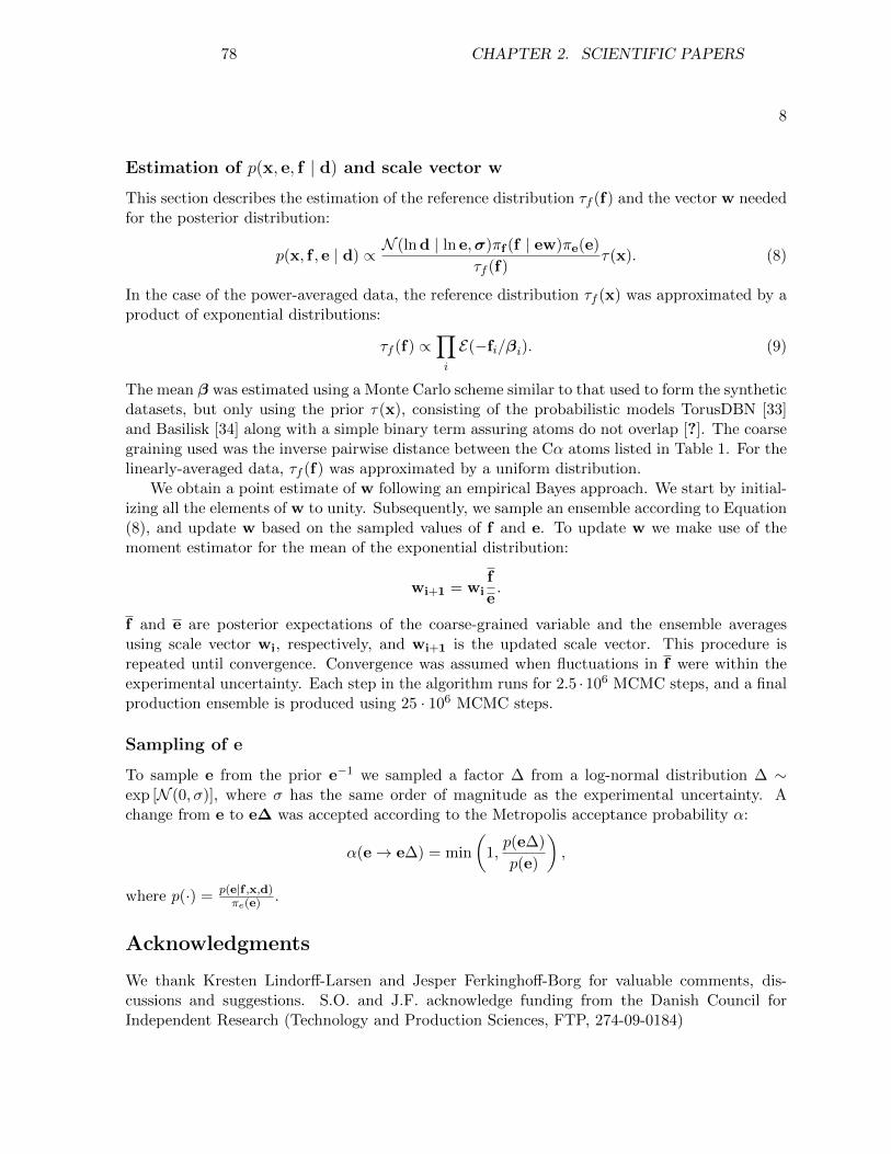
8

Estimation of p(x, e, f | d) and scale vector w

This section describes the estimation of the reference distribution τf (f) and the vector w neededfor the posterior distribution:

p(x, f , e | d) ∝ N (ln d | ln e,σ)πf (f | ew)πe(e)

τf (f)τ(x). (8)

In the case of the power-averaged data, the reference distribution τf (x) was approximated by aproduct of exponential distributions:

τf (f) ∝∏

i

E(−fi/βi). (9)

The mean β was estimated using a Monte Carlo scheme similar to that used to form the syntheticdatasets, but only using the prior τ(x), consisting of the probabilistic models TorusDBN [33]and Basilisk [34] along with a simple binary term assuring atoms do not overlap [?]. The coarsegraining used was the inverse pairwise distance between the Cα atoms listed in Table 1. For thelinearly-averaged data, τf (f) was approximated by a uniform distribution.

We obtain a point estimate of w following an empirical Bayes approach. We start by initial-izing all the elements of w to unity. Subsequently, we sample an ensemble according to Equation(8), and update w based on the sampled values of f and e. To update w we make use of themoment estimator for the mean of the exponential distribution:

wi+1 = wif

e.

f and e are posterior expectations of the coarse-grained variable and the ensemble averagesusing scale vector wi, respectively, and wi+1 is the updated scale vector. This procedure isrepeated until convergence. Convergence was assumed when fluctuations in f were within theexperimental uncertainty. Each step in the algorithm runs for 2.5 ·106 MCMC steps, and a finalproduction ensemble is produced using 25 · 106 MCMC steps.

Sampling of e

To sample e from the prior e−1 we sampled a factor ∆ from a log-normal distribution ∆ ∼exp [N (0, σ)], where σ has the same order of magnitude as the experimental uncertainty. Achange from e to e∆ was accepted according to the Metropolis acceptance probability α:

α(e→ e∆) = min

(1,p(e∆)

p(e)

),

where p(·) = p(e|f ,x,d)πe(e)

.

Acknowledgments

We thank Kresten Lindorff-Larsen and Jesper Ferkinghoff-Borg for valuable comments, dis-cussions and suggestions. S.O. and J.F. acknowledge funding from the Danish Council forIndependent Research (Technology and Production Sciences, FTP, 274-09-0184)


9

References

1. Brunger AT, Nilges M (1993) Computational challenges for macromolecular structuredetermination by X-ray crystallography and solution NMR spectroscopy. Q Rev Biophys26: 49–125.

2. Jardetzky O (1980) On the nature of molecular conformations inferred from high-resolution NMR. Biochim Biophys Acta 621: 227 - 232.

3. Jack A, Levitt M (1978) Refinement of large structures by simultaneous minimization ofenergy and R factor. Acta Crystallogr A 34: 931–935.

4. Rieping W, Habeck M, Nilges M (2005) Inferential structure determination. Science 309:303–306.

5. Habeck M (2011) Statistical mechanics analysis of sparse data. J Struct Biol 173: 541–548.

6. Torda AE, Scheek RM, van Gunsteren WF (1989) Time-dependent distance restraints inmolecular dynamics simulations. Chem Phys Lett 157: 289 - 294.

7. Torda AE, Scheek RM, van Gunsteren WF (1990) Time-averaged nuclear overhauser effectdistance restraints applied to tendamistat. J Mol Biol 214: 223 - 235.

8. Lindorff-Larsen K, Kristjansdottir S, Teilum K, Fieber W, Dobson CM, et al. (2004)Determination of an ensemble of structures representing the denatured state of the bovineacyl-coenzyme a binding protein. J Am Chem Soc 126: 3291-3299.

9. Kim Y, Prestegard JH (1989) A dynamic model for the structure of acyl carrier proteinin solution. Biochemistry 28: 8792-7.

10. Teilum K, Olsen JG, Kragelund BB (2011) Protein stability, flexibility and function.Biochim Biophys Acta 1814: 969-976.

11. Jha AK, Colubri A, Freed KF, Sosnick TR (2005) Statistical coil model of the unfoldedstate: Resolving the reconciliation problem. Proc Natl Acad Sci USA 102: 13099-13104.

12. Bernado P, Blanchard L, Timmins P, Marion D, Ruigrok RWH, et al. (2005) A struc-tural model for unfolded proteins from residual dipolar couplings and small-angle x-rayscattering. Proc Natl Acad Sci USA 102: 17002-17007.

13. Chen Y, Campbell SL, Dokholyan NV (2007) Deciphering protein dynamics from NMRdata using explicit structure sampling and selection. Biophys J 93: 2300 - 2306.

14. Nodet G, Salmon L, Ozenne V, Meier S, Jensen MR, et al. (2009) Quantitative descriptionof backbone conformational sampling of unfolded proteins at amino acid resolution fromNMR residual dipolar couplings. J Am Chem Soc 131: 17908-17918.


10

15. Bertini I, Giachetti A, Luchinat C, Parigi G, Petoukhov MV, et al. (2010) Conformationalspace of flexible biological macromolecules from average data. J Am Chem Soc 132: 13553-13558.

16. Fisher CK, Huang A, Stultz CM (2010) Modeling intrinsically disordered proteins withbayesian statistics. J Am Chem Soc 132: 14919-14927.

17. Kemmink J, van Mierlo CP, Scheek RM, Creighton TE (1993) Local structure due to anaromatic-amide interaction observed by 1H-nuclear magnetic resonance spectroscopy inpeptides related to the n terminus of bovine pancreatic trypsin inhibitor. J Mol Biol 230:312 - 322.

18. Lindorff-Larsen K, Best RB, DePristo MA, Dobson CM, Vendruscolo M (2005) Simulta-neous determination of protein structure and dynamics. Nature 433: 128-132.

19. Groth M, Malicka J, Czaplewski C, O ldziej S, Lankiewicz L, et al. (1999) Maximum en-tropy approach to the determination of solution conformation of flexible polypeptidesby global conformational analysis and NMR spectroscopy–application to DNS1-c-[D-A2,bu2,Trp4,Leu5]enkephalin and DNS1-c-[D-A2bu2,Trp4,D-Leu5]enkephalin. J BiomolNMR 15: 315-30.

20. Bonvin AMJJ, Boelens R, Kaptein R (1994) Time- and ensemble-averaged direct NOErestraints. J Biomol NMR 4: 143-149.

21. Pitera JW, Chodera JD (2012) On the use of experimental observations to bias simulatedensembles. J Chem Theory Comput 8: 3445.

22. Cavalli A, Camilloni C, Vendruscolo M (2013) Molecular dynamics simulations withreplica-averaged structural restraints generate structural ensembles according to the max-imum entropy principle. J Chem Phys 138: 094112.

23. Irback A, Mitternacht S, Mohanty S (2009) An effective all-atom potential for proteins.PMC Biophys 2: 2.

24. Cavanagh J, Fairbrother WJ, III AGP, Skelton NJ, Rance M (2006) Protein NMR Spec-troscopy: Principles And Practice. Academic Press, 2 edition.

25. Hamelryck T, Borg M, Paluszewski M, Paulsen J, Frellsen J, et al. (2010) Potentials ofmean force for protein structure prediction vindicated, formalized and generalized. PLoSOne 5: e13714.

26. Hamelryck T, Mardia K, Ferkinghoff-Borg J, editors (2012) Bayesian Methods in Struc-tural Bioinformatics. Springer.

27. Kullback S (1968) Information Theory and Statistics. Dover.

28. McCullagh P, Nelder JA (1989) Generalized linear models. Chapman & Hall, London, 2edition.


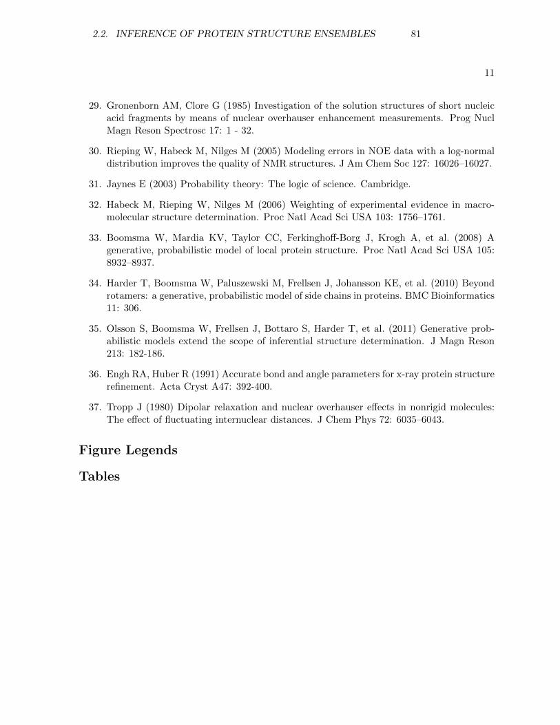
11

29. Gronenborn AM, Clore G (1985) Investigation of the solution structures of short nucleicacid fragments by means of nuclear overhauser enhancement measurements. Prog NuclMagn Reson Spectrosc 17: 1 - 32.

30. Rieping W, Habeck M, Nilges M (2005) Modeling errors in NOE data with a log-normaldistribution improves the quality of NMR structures. J Am Chem Soc 127: 16026–16027.

31. Jaynes E (2003) Probability theory: The logic of science. Cambridge.

32. Habeck M, Rieping W, Nilges M (2006) Weighting of experimental evidence in macro-molecular structure determination. Proc Natl Acad Sci USA 103: 1756–1761.

33. Boomsma W, Mardia KV, Taylor CC, Ferkinghoff-Borg J, Krogh A, et al. (2008) Agenerative, probabilistic model of local protein structure. Proc Natl Acad Sci USA 105:8932–8937.

34. Harder T, Boomsma W, Paluszewski M, Frellsen J, Johansson KE, et al. (2010) Beyondrotamers: a generative, probabilistic model of side chains in proteins. BMC Bioinformatics11: 306.

35. Olsson S, Boomsma W, Frellsen J, Bottaro S, Harder T, et al. (2011) Generative prob-abilistic models extend the scope of inferential structure determination. J Magn Reson213: 182-186.

36. Engh RA, Huber R (1991) Accurate bond and angle parameters for x-ray protein structurerefinement. Acta Cryst A47: 392-400.

37. Tropp J (1980) Dipolar relaxation and nuclear overhauser effects in nonrigid molecules:The effect of fluctuating internuclear distances. J Chem Phys 72: 6035–6043.

Figure Legends

Tables


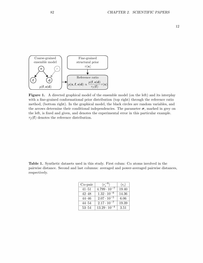
12

Reference ratio

Fine-grainedstructural prior

p(x, f , e|d) ∝ p(f , e|d)τf (f)

τ(x)

τ(x)

d

e

f

σ

Coarse-grainedensemble model

p(f , e|d)

Figure 1. A directed graphical model of the ensemble model (on the left) and its interplaywith a fine-grained conformational prior distribution (top right) through the reference ratiomethod, (bottom right). In the graphical model, the black circles are random variables, andthe arrows determine their conditional independencies. The parameter σ, marked in grey onthe left, is fixed and given, and denotes the experimental error in this particular example.τf (f) denotes the reference distribution.

Table 1. Synthetic datasets used in this study. First colum: Cα atoms involved in thepairwise distance. Second and last columns: averaged and power-averaged pairwise distances,respectively.

Cα-pair 〈r−6i 〉〈ri〉41–51 4.799 · 10−7 19.40

42–48 1.32 · 10−6 14.36

44–46 2.07 · 10−5 6.06

44–54 2.17 · 10−7 19.39

53–54 13.29 · 10−4 3.51


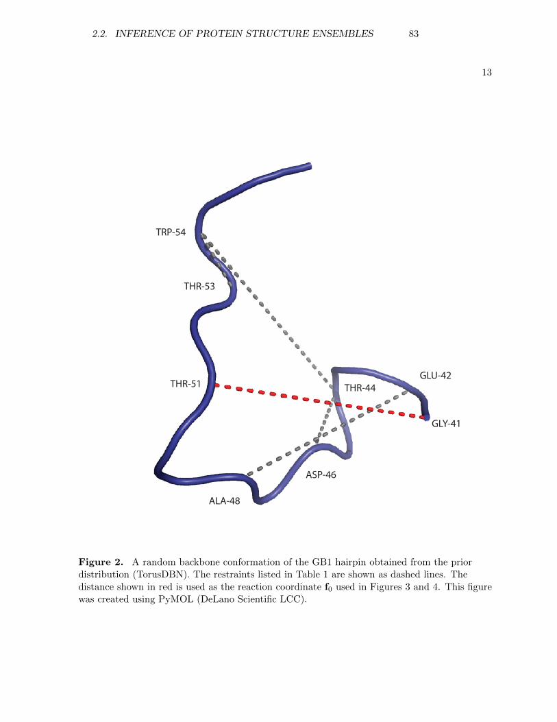
13

TRP-54

THR-53

THR-51

ALA-48

ASP-46

THR-44

GLU-42

GLY-41

Figure 2. A random backbone conformation of the GB1 hairpin obtained from the priordistribution (TorusDBN). The restraints listed in Table 1 are shown as dashed lines. Thedistance shown in red is used as the reaction coordinate f0 used in Figures 3 and 4. This figurewas created using PyMOL (DeLano Scientific LCC).


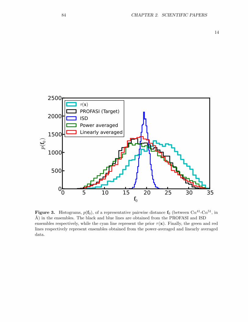
14

0 5 10 15 20 25 30 35f0

0

500

1000

1500

2000

2500

p(f

0)

τ(x)

PROFASI (Target)

ISD

Power averaged

Linearly averaged

Figure 3. Histograms, p(f0), of a representative pairwise distance f0 (between Cα41-Cα51, inA) in the ensembles. The black and blue lines are obtained from the PROFASI and ISDensembles respectively, while the cyan line represent the prior τ(x). Finally, the green and redlines respectively represent ensembles obtained from the power-averaged and linearly averageddata.


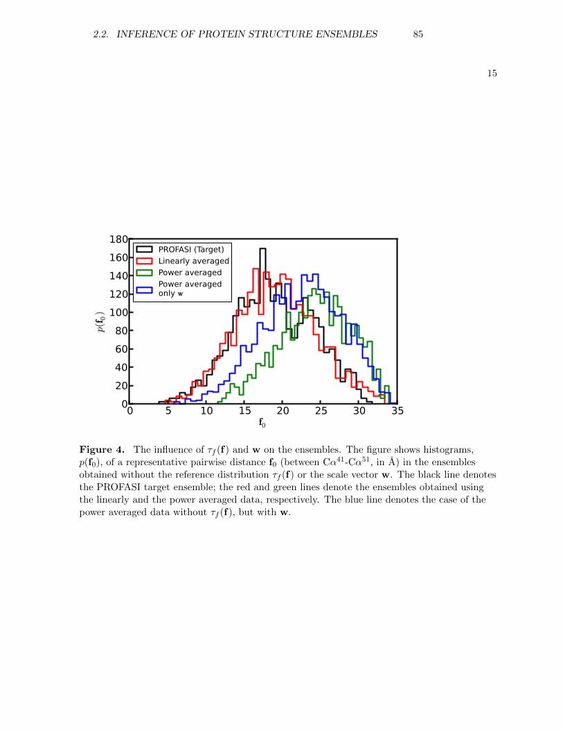
15

0 5 10 15 20 25 30 35f0

0

20

40

60

80

100

120

140

160

180

p(f

0)

PROFASI (Target)

Linearly averaged

Power averaged

Power averagedonly w

Figure 4. The influence of τf (f) and w on the ensembles. The figure shows histograms,p(f0), of a representative pairwise distance f0 (between Cα41-Cα51, in A) in the ensemblesobtained without the reference distribution τf (f) or the scale vector w. The black line denotesthe PROFASI target ensemble; the red and green lines denote the ensembles obtained usingthe linearly and the power averaged data, respectively. The blue line denotes the case of thepower averaged data without τf (f), but with w.



2.3 Construction of protein structure ensembles in con-tinuous space through minimal biasing of a simplephysical force field.

The study of concerted motions in proteins is an inherently difficult task.This type of motion occur on timescales which are difficult reach directly inexperiment and unrestrained simulations. In this paper we seek use a coarse,yet efficient, forcefield restrained by a modestly sized set of local geometricRDC restraints to study the native ensemble of the third immunoglobulinbinding domain of protein G (GB3). We achieve this by using our previouslyproposed hierarchical restraining strategy.

We find that the restrained ensembles obtained in this procedure agreewith complementary experimental data significantly better than the unre-strained ensemble. This cross-validation considers data reflecting both oflocal and non-local geometric features. In addition we find that previouslyreported dynamic properties are accurately reproduced. Finally, we find astrong anti-correlated motion which may be attributed to the binding GB3sendogenous partner, Fab.

Collectively, these results suggest that we are able to construct realisticdistributions of protein structure using comparably small datasets of localgeometric restraints by complementing by simplistic forcefields. This mayprove to be a powerful technique to allow for the study of concerted motionsusing accurate local restraints.This is a first-author paper and I was involved in all aspects of the work.Unsubmitted manuscript.

Construction of protein structure ensembles incontinuous space through minimal biasing of asimple physical force field.Simon Olsson, ∗ and Thomas Hamelryck ∗

∗Bioinformatics Centre, Department of Biology, Faculty of Science, University of Copenhagen, Denmark

draft manuscript

The structural motion of biological molecules is tightly coupled totheir endogenous functions. However, while the study of fast mo-tions has become increasingly feasible in recent years, the study ofslower, biologically important, motions remains confined to particu-larly tractable systems. Here we present a native ensemble of theextensively studied third immunoglobulin binding domain of proteinG (GB3). We use an efficient, yet coarse, force field restrained bya modestly sized data-set in a minimally biased fashion to accu-rately describe both local and non-local conformational dynamics.The resulting ensemble is in agreement with previous studies thatrely on much more elaborate datasets. In addition, we find a pre-viously unreported anti-correlated motion between the β-sheet andthe α-helix. GB3 appears to undergo a similar anti-correlated motionwhen it binds its endogenous partner, Fab. These results suggestthat we are able to construct realistic conformational ensembles ofbiomolecules in continuous space very efficiently. In a more gen-eral setting, this approach may allow for a dramatic reduction in thecomputational as well as experimental resources needed to obtainaccurate models of conformational dynamics in biomolecules.

probabilistic models | protein ensembles | restrained simulations | information

theory

Abbreviations: MMLP, Mean minus log posterior probability; GB3, third immunoglob-

ulin binding domain of protein G; RDCs, residual dipolar couplings; HBC, hydrogen

bond scalar couplings; EM, expectation maximization; eNOE, exact nuclear Over-

hauser enhancement; MCMC, Markov chain Monte Carlo

Under physiological conditions the motions of proteinsspan several spatial and temporal orders of magnitude.

Fast and, in particular, slow molecular motions are essentialto obtain, sustain and regulate biological functions which in-clude signal transduction [1] and catalysis [2]. The studyof fast molecular motions may be routinely performed us-ing experimental [3] or computational [4] means. Slowermotions are, however, notoriously difficult to investigate [5].Computationally, such studies require either special purposesuper-computers or extensive datasets for unrestrained andrestrained simulations respectively [6, 7]. Experimental tech-niques such as relaxation dispersion allow extraction of ther-modynamical, structural (chemical) and kinetic informationabout the exchange between states [8]. However, these exper-iments are only sensitive provided that the chemical environ-ment is modulated significantly by this motion [9].

Residual dipolar couplings (RDCs) provide geometric in-formation averaged over many time scales (up to ms) andmay be used to study the slow molecular motions of proteins[10]. Such an application of RDCs has already been subjectto extensive research [6, 11, 12]. Several reports describe fit-ting of discrete sets of conformations to large experimentaldatasets [12], performing restrained simulations and select-ing sets of protein conformations post hoc to describe struc-tural variability in folded and intrinsically disordered proteins[13, 14]. Common to these procedures is the assumption thatmotion reflected in the data is accurately represented by aweighted average of a discrete set of molecular conformations.

Potential problems in these methodologies have been pointedout previously [15, 16].

In this work, we studied the native ensemble of the thirdimmunoglobulin binding domain of protein G (GB3). Wecurated a modestly sized dataset of from RDCs obtainedthrough structurally conservative mutagenesis of charged sur-face residues that were reported previously [17]. Such mu-tations are common and thus this dataset represents a casewhich may be easily reproducible for other systems. The datafor the different mutants give complementary views of theN-HN and Cα-Hα bonds in the protein backbone of GB3 –something which may be difficult to achieve by solely chang-ing alignment media [18]. In principle, the method is appli-cable to data sets collected under less alignment conditions ifRDCs between other nuclei are included. We used these as re-straints in a native simulation using the Profasi forcefield [19].We utilized our previously described strategy to impose theminimal necessary bias on the forcefield to be in accord withnoisy experimental data [16]. We devised a robust algorithmto iteratively refine the bias with guaranteed convergence infinite time. We found that the restrained ensemble accuratelyreproduces complementary experimental data not used to re-strain the simulations. Furthermore, we found that the localcorrelated motions present in the unrestrained ensemble werenot significantly distorted by our restraining procedure andwere in agreement with what has been previously suggested[6, 20]. Finally, we found strong anti-correlated motion be-tween the α-helix and the β-sheet in our restrained ensemble.This motion is consistent with the conformational differencebetween GB3 in its free state and when it is bound to itsendogenous partner.

These results indicate that efficient, yet coarse, forcefields,when appropriately restrained by modestly sized datasets,may be used to obtain accurate native ensembles. These sim-ulations are computationally inexpensive, even on commod-ity hardware, dramatically reducing the computational andexperimental resources necessary to obtain accurate descrip-tions of the native fluctuations in biomolecular systems. Thismay in turn allow for rigorous large-scale studies of dynamicsin biomolecules.

Reserved for Publication Footnotes

PNAS Issue Date Volume Issue Number 1–6

2.3. CONTINUOUS ENSEMBLES OF PROTEINS 87

ResultsKullback-Leibler optimal restraining of force fields.Our aim is to use the computationally efficient forcefield Pro-fasi in a native ensemble simulation restrained by experimen-tal observations, which are subject to experimental noise, aswell as spatial and temporal averaging. The experimentaldataset we use here is relatively small compared to what hasbeen used previously [6, 20]. Consequently, it will not be suf-ficiently informative to provide an accurate description of thenative ensemble of structures devoid of any prior assumptions.Similarly, the forcefield Profasi only provides a simplified viewof the conformational distribution of the protein. Therefore,we seek to restrain Profasi using our data in a minimally bias-ing way. This may be achieved by considering the restrainingproblem as a problem of Kullback-Leibler optimization. Thiscorresponds imposing the minimal bias on our prior distribu-tion π(x) (the Boltzmann ensemble of the Profasi forcefield)

in order for the average f of the instantaneous representationf to match our data within the experimental uncertainty. Wehave previously described a general way of performing thisoptimization in our current context, temporally and spatiallyaverage data subject to experimental uncertainty [16].

We have the posterior distribution,

p(f , e,x | d) ∝ p(d | e, σ)πf (f | e)πx(x)πe(e) [1]

where f denotes an instantaneous coarse grained representa-tion (’back-calculated experimental data’) of a protein struc-ture x; e represents an ensemble average of this coarse grain-ing, and d represents an experimental observation consistentwith this particular coarse-graining. Here we use a normal dis-tribution, N (·), for the likelihood p(d | e, σ), and a log-linearmodel G(·) for the prior πf (f | e). The likelihood N (d | e, σ)models the probability of the experimental data given its un-certainty σ and some unknown ensemble average. The priorG(f | V, e) models the distribution of protein conformationsgiven the ensemble average and the scale matrix V. Finally,we chose an uniform prior for the ensemble average, π(e) ∝ 1.The hierarchical structure of this model was previously de-scribed [16]. However, the specific distributions have beenadjusted to be in accord with the current experimental data.Please find further details on the model in the Materials andMethods section below.

We wish to obtain a point estimate of the unknown (la-tent) scale matrix V such that a given e yields a posteriorexpectation of f according to eq. 1 which is exactly e. Thiscorresponds to imposing the least necessary bias to the priordistribution of protein conformations to fulfill the experimen-tal data. We here devise an EM algorithm to carry out this es-timation (see Materials and Methods). Additionally, we makeuse of a new method to model to account for the different ex-perimental alignment conditions of the datasets (see Materialsand Methods).

Expectation maximization algorithm yields minimallybiased native ensembles To investigate the native ensem-ble of GB3 we use eight sets of previously reported resid-ual dipolar couplings (RDCs) [17] to restrain the forcefieldProfasi [19]. The data was acquired in seven different align-ment conditions, by using structurally conserved mutantsK19AD47K, K19ED40N, K19AT11K, K19EK4A, and twowhich include a C- and N-terminal His-tag, K19EK4A-C-His6,and K19EK4A-N-His6 along with the wildtype of GB3. Sevenof the datasets reported on the N-HN bond whereas one re-ported on the Cα-Hα bond. These conditions have been shownto accurately map the five independent parameters associatedwith molecular alignment [21]. Consequently, using appro-

priate structural prior information these datasets should veryaccurately describe the fluctuations of the N-HN bond andthe Cα-Hα bond, albeit to a lesser extent.

We used an EM algorithm [22] to iteratively refine re-strained native ensembles of GB3 (EMi for i = 0 . . . 7). Wefind that agreement with the training data (declining Q-factor) correlates with the increase in expected posterior prob-ability (decline in MMLP) of the model (Fig. 1) and agree-ment with complementary data not used in the restraining(see Supplementary Material). The final restrained ensemble(EM7) is stable near the native state of GB3, with consider-able flexibility. In contrast, the unrestrained ensemble (EM0)partially unfolds during simulation, see Table 1.

Realistic local and non-local dynamics. While it ispromising that the restrained ensemble, EM7, displays consid-erable flexibility and is in good agreement with the trainingdata (Q = 15%), it does not assure physical realism. We areable to test the quality of EM7 by cross-validation with thewealth of experimental data available for GB3, providing lo-cal and non-local geometrical information. We compared thereproduction of the experimental data to two previously pub-lished models of GB3: 2LUM, an ensemble refined using exactnuclear Overhauser enhancements (eNOEs), scalar couplings,RDCs and chemical shifts [20] and 2OED a RDC refined x-raystructure [23].

As shown in Table 1, EM7 is in excellent agreement withpreviously reported scalar couplings [24] and previously un-published cross-correlated dipolar relaxation rates. The unre-strained EM0 ensemble, in general, is of considerably worsequality. Compared to the previously published models ofGB3, 2LUM and 2OED, agreement is comparable. In partic-ular, it is striking that EM7 shows slightly better quantitative3JHN−Cβ agreement when compared to the 2LUM ensemble,where these data were used in the refinement process. Thecross-correlated dipolar relaxation rates RHNi−HNi+1 are par-

ticularly sensitive to an accurate representation of the N-HN

bond [25, 26]. We see a dramatic improvement in the corre-lation with these data when comparing the restrained to theunrestrained ensemble. This suggests that the RDCs used torestrain the Profasi forcefields indeed accurately describe thefluctuations of the N-HN bonds.

The non-local dynamics were evaluated by cross valida-tion with stereospecifically assigned exact nuclear Overhauserenhancements (eNOEs) and hydrogen bond scalar couplings(HBCs). As with the scalar couplings above, the 2LUM en-semble was refined against the eNOE data. However, here thisensemble generally showed the correlation with these data.This is the case both when the conformational exchange isassumed to be much faster (eNOE−3) or slower (eNOE−6)than the molecular tumbling [27]. The RDC refined structure,2OED, shows slightly worse agreement while the restrained(EM7) and unrestrained (EM0) Profasi ensembles are approx-imately 10% and 20% worse when compared to 2LUM. Sur-prisingly, the agreement with the hydrogen bond scalar cou-plings is quantitatively best in the restrained Profasi ensembleEM7, closely followed by 2OED, 2LUM and the unrestrainedensemble. This result, in particular, is interesting because theHBCs report long-range correlated motions [28] averaged onthe same timescale as RDCs [29]. Collectively, these resultssuggest that the local and non-local dynamics in EM7 are ofgood quality.

DiscussionConcerted motions in the minimally biased ensemblemay suggest a conformational selection binding mech-

2 Footline Author


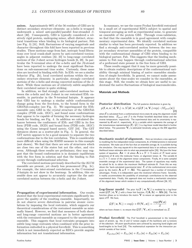
anism. Approximately 90% of the 56 residues of GB3 are indistinct secondary structure elements: an α-helix is wrappedunderneath a mixed anti-parallel/parallel four-stranded β-sheet [30]. Consequently, GB3 is typically considered a rel-atively rigid protein, undergoing minor, albeit distinct, struc-tural transitions when binding to its biological partner, Fab(see Fig. 3) [31]. Still, fluctuations of varying magnitude andcharacter throughout this fold have been reported in previousstudies. These motions range from fast, isotropic bond libera-tions over local crank-shaft moves by anti-correlated torsion-angles in adjacent residues [32, 33] to long-range correlatedmotions of the β-sheet across hydrogen bonds [6, 20]. In par-ticular the N-terminal sites of the α-helix and the β2-strandhave been reported to undergo the most significant fluctua-tions on sub-nanosecond time scales. Curiously, these samesites are involved in binding with Fab. In EM7 we see a similarbehavior (Fig. 2b), local correlated motions within the sec-ondary structure elements: in particular, strongly correlatedmotions of the α-helix and strong concerted motions of the β-sheet. While these motions are of relatively subtle amplitudetheir correlated nature is quite striking.

In addition, we find strongly anti-correlated motions be-tween the α-helix and the β-sheet in our restrained EM7 en-semble, in particular in the N-terminal hairpin. It appearsthat GB3 has to undergo a similar subtle conformationalchange going from the free-form, to the bound form in theGB3:Fab-complex (see Fig. 3). We superimposed the EM7

ensemble onto GB3 in the crystal structure of the GB3:Fabcomplex (PDB code, 1IGC), and found some conformationsthat appear to be capable of forming the necessary hydrogenbonds for binding, see Fig. 4. In addition we calculated dis-tances between the conformers of EM7 and GB3 in its freeform (PDB code, 1IGD) and bound form (PDB code, 1IGC)using the Gauss integral based metric, GIT [34]. The GITdistances shown as a scatter-plot in Fig. 5. In general, theGIT metric appears to be a good measure to separate the twoconformations due to the low correlation. This is considerablymore difficult when using the RMSD measure in this example(not shown). We find that there are sets of structures whichare close two one of the states but not the other, and viceversa. Although these results are preliminary, they may sug-gest that the bound conformation is in dynamic equilibriumwith the free form in solution and that the binding to Faboccurs through conformational selection.

The correlated motions previously described for the 2LUMensemble are present, yet clearly less pronounced (Fig. 2c).For example, the inter-strand correlations in the C-terminalβ-hairpin do not show in the heatmap. In addition, this en-semble does not appear to accurately capture the the anti-correlated motion between the α-helix and the β-sheet.

Propagation of experimental information. Our resultsshowed that the local experimental restraints significantly im-prove the quality of the resulting ensemble. Importantly, wedo not observe severe distortions in pairwise atomic corre-lations by imposing the local restraints, which supports ourtheoretical considerations of the restrained ensemble as mini-mally biased. However, we find that measures of both short-and long-range concerted motions are in better agreementwith the restrained ensemble as compared to the unrestrainedensemble. This suggests that local restraints propagate intosubtle long range restraints when combined with the prior in-formation embodied in a physical forcefield. This is somethingwhich is not immediately expected as RDCs provide angularinformation but not translational information.

In summary, we use the coarse Profasi forcefield restrainedby a small set of experimental RDCs subject to spatial andtemporal averaging as well as experimental noise, to generatean ensemble of the protein GB3. Through cross-validation,we find that the ensemble is in good agreement with comple-mentary experimental data. We identify correlated motionssimilar to what has been previously reported. In addition wefind a strongly anti-correlated motion between the two ma-jor secondary structure assemblies of the protein, compatiblewith the conformational change of GB3 when binding to itsbiological partner, Fab. This suggests that the binding mech-anism to Fab may happen through conformational selectionof a preformed state present in the free form of GB3.

These results suggest that it may be more generally possi-ble to obtain realistic descriptions of the conformational vari-ability through minimal biasing of native ensembles simula-tion of simple forcefields. In general, we cannot make assess-ments about the time-scales we consider in the ensembles, atthis stage. Still, the results we obtain here are useful to un-derstand the native fluctuations of biological macromolecules.

Materials and Methods

Posterior distribution The full posterior distribution is given by,

p(f , e,x | d,Vi) ∝ N (d | e, σ)G(f | e,Vi) exp(−βEprof(x))[ 2 ]

where f is calculated from a conformational micro-state x using the alignment model

described below. Eprof and β is the Profasi forcefield described below and the

inverse temperature, respectively. The experimental data and its uncertainty is rep-

resented by d and σ, respectively. e is a variable which represents the average of

the instantaneous representations (f ). G(·) is a log-linear model described in further

detail below. The parameter Vi is estimated iteratively using an the EM algorithm

described below.

Stochastic model of alignment. Here we introduce a new approach

to modeling the five independent tensor components, s, of folded proteins in restrained

simulations. We make use of the fact that an ensemble average, e, is available during

the simulation. One may equate e to the experimental data in an ordinary maximum

likelihood tensor estimator akin to what was presented earlier [35]. We have the linear

system of equations, As = e where A is a N × 5 matrix of N bond vector

projections of x onto the molecular frame, or alignment tensor, s. The variable sis a 5 × 1 vector of the alignment tensor components. Finally, e is some sampled

ensemble average of the experimental data. The system of equations may readily

be solved for s, to obtain the maximum likelihood estimate s. From this we may

obtain the ’back-calculated experimental data’, f , of the conformational micro-state

given by the matrix A as f = As. This approach has a number of immediate

advantages. Firstly, it is independent upon the rotational reference frame. Secondly,

it readily accommodates the possibility of anisotropic contributions to the observed

experimental data. Finally, this approach does not involve a mechanistic simulation

of the alignment tensor which renders it very computationally efficient [36, 37].

Log-linear model The prior πf (f | e,Vi) is modeled by a log-linear

model G(f | e,Vi) with a linear link function, `(A,b) = Ab [38]. The link

function allows us to introduce the matrix V to ensure an appropriate prior in the

space of f . We have,

G(f | e,Vi) = exp[c+ f`(Vi, e)] =exp(fVie)

Z [ 3 ]

where we have chosen c, to ensure that G(f | Vi, e) is normalized via Z .

Profasi forcefield The Prof forcefield is parameterized in the torsional

space of protein, eg. the φ and ψ torsion angles of the backbone and χ-torsions

of the sidechain. All-atom specifications were achieved by assuming bond-angles and

bond-lengths to be fixed [19]. The mathematical expression for the interaction po-

tential consists of four terms

Eprofasi(x) = Eloc(x) + Eev(x) + Ehb(x) + Esc(x)

Footline Author PNAS Issue Date Volume Issue Number 3


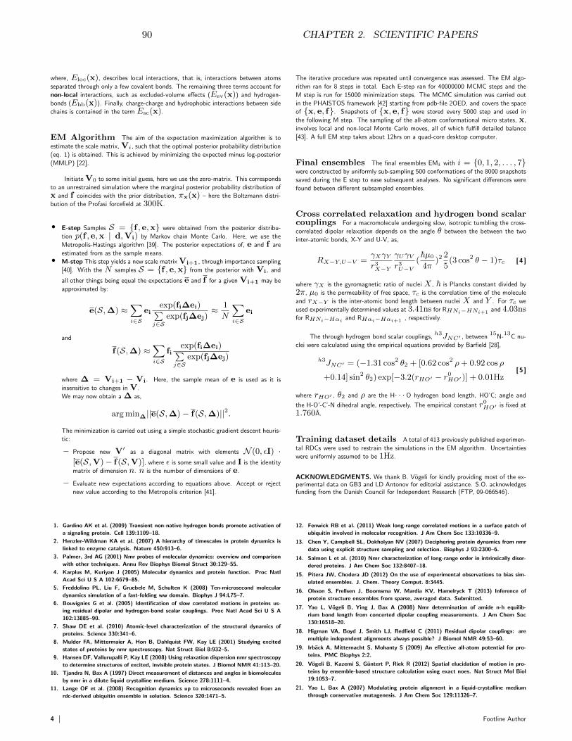
where, Eloc(x), describes local interactions, that is, interactions between atoms

separated through only a few covalent bonds. The remaining three terms account for

non-local interactions, such as excluded-volume effects (Eev(x)) and hydrogen-

bonds (Ehb(x)). Finally, charge-charge and hydrophobic interactions between side

chains is contained in the term Esc(x).

EM Algorithm The aim of the expectation maximization algorithm is to

estimate the scale matrix, Vi, such that the optimal posterior probability distribution

(eq. 1) is obtained. This is achieved by minimizing the expected minus log-posterior

(MMLP) [22].

Initiate V0 to some initial guess, here we use the zero-matrix. This corresponds

to an unrestrained simulation where the marginal posterior probability distribution of

x and f coincides with the prior distribution, πx(x) – here the Boltzmann distri-

bution of the Profasi forcefield at 300K.

• E-step Samples S = {f , e,x} were obtained from the posterior distribu-

tion p(f , e,x | d,Vi) by Markov chain Monte Carlo. Here, we use the

Metropolis-Hastings algorithm [39]. The posterior expectations of, e and f are

estimated from as the sample means.• M-step This step yields a new scale matrix Vi+1, through importance sampling

[40]. With the N samples S = {f , e,x} from the posterior with Vi, and

all other things being equal the expectations e and f for a given Vi+1 may be

approximated by:

e(S,∆) ≈∑

i∈Sei

exp(fi∆ei)∑j∈S

exp(fj∆ej)≈ 1

N

∑

i∈Sei

and

f(S,∆) ≈∑

i∈Sfi

exp(fi∆ei)∑j∈S

exp(fj∆ej)

where ∆ = Vi+1 − Vi. Here, the sample mean of e is used as it is

insensitive to changes in V.

We may now obtain a ∆ as,

arg min∆||e(S,∆)− f(S,∆)||2.

The minimization is carried out using a simple stochastic gradient descent heuris-

tic:

– Propose new V′ as a diagonal matrix with elements N (0, εI) ·[e(S,V)− f(S,V)], where ε is some small value and I is the identity

matrix of dimension n. n is the number of dimensions of e.

– Evaluate new expectations according to equations above. Accept or reject

new value according to the Metropolis criterion [41].

The iterative procedure was repeated until convergence was assessed. The EM algo-

rithm ran for 8 steps in total. Each E-step ran for 40000000 MCMC steps and the

M step is run for 15000 minimization steps. The MCMC simulation was carried out

in the PHAISTOS framework [42] starting from pdb-file 2OED, and covers the space

of {x, e, f}. Snapshots of {x, e, f} were stored every 5000 step and used in

the following M step. The sampling of the all-atom conformational micro states, x,

involves local and non-local Monte Carlo moves, all of which fulfill detailed balance

[43]. A full EM step takes about 12hrs on a quad-core desktop computer.

Final ensembles The final ensembles EMi with i = {0, 1, 2, . . . , 7}were constructed by uniformly sub-sampling 500 conformations of the 8000 snapshots

saved during the E step to ease subsequent analyses. No significant differences were

found between different subsampled ensembles.

Cross correlated relaxation and hydrogen bond scalarcouplings For a macromolecule undergoing slow, isotropic tumbling the cross-

correlated dipolar relaxation depends on the angle θ between the between the two

inter-atomic bonds, X-Y and U-V, as,

RX−Y,U−V =γXγYr3X−Y

γUγVr3U−V

(~µ0

4π)2

2

5(3 cos2 θ − 1)τc [ 4 ]

where γX is the gyromagnetic ratio of nuclei X , ~ is Plancks constant divided by

2π, µ0 is the permeability of free space, τc is the correlation time of the molecule

and rX−Y is the inter-atomic bond length between nuclei X and Y . For τc we

used experimentally determined values at 3.41ns for RHNi−HNi+1 and 4.03nsfor RHNi−Hαi and RHαi−Hαi+1 , respectively.

The through hydrogen bond scalar couplings,h3JNC′ , between

15N-

13C nu-

clei were calculated using the empirical equations provided by Barfield [28],

h3JNC′ = (−1.31 cos2 θ2 + [0.62 cos2 ρ+ 0.92 cos ρ

+0.14] sin2 θ2) exp[−3.2(rHO′ − r0HO′)] + 0.01Hz[ 5 ]

where rHO′ , θ2 and ρ are the H· · ·O hydrogen bond length, HO’C; angle and

the H-O’-C’-N dihedral angle, respectively. The empirical constant r0HO′ is fixed at

1.760A.

Training dataset details A total of 413 previously published experimen-

tal RDCs were used to restrain the simulations in the EM algorithm. Uncertainties

were uniformly assumed to be 1Hz.

ACKNOWLEDGMENTS. We thank B. Vogeli for kindly providing most of the ex-perimental data on GB3 and LD Antonov for editorial assistance. S.O. acknowledgesfunding from the Danish Council for Independent Research (FTP, 09-066546).

1. Gardino AK et al. (2009) Transient non-native hydrogen bonds promote activation of

a signaling protein. Cell 139:1109–18.

2. Henzler-Wildman KA et al. (2007) A hierarchy of timescales in protein dynamics is

linked to enzyme catalysis. Nature 450:913–6.

3. Palmer, 3rd AG (2001) Nmr probes of molecular dynamics: overview and comparison

with other techniques. Annu Rev Biophys Biomol Struct 30:129–55.

4. Karplus M, Kuriyan J (2005) Molecular dynamics and protein function. Proc Natl

Acad Sci U S A 102:6679–85.

5. Freddolino PL, Liu F, Gruebele M, Schulten K (2008) Ten-microsecond molecular

dynamics simulation of a fast-folding ww domain. Biophys J 94:L75–7.

6. Bouvignies G et al. (2005) Identification of slow correlated motions in proteins us-

ing residual dipolar and hydrogen-bond scalar couplings. Proc Natl Acad Sci U S A

102:13885–90.

7. Shaw DE et al. (2010) Atomic-level characterization of the structural dynamics of

proteins. Science 330:341–6.

8. Mulder FA, Mittermaier A, Hon B, Dahlquist FW, Kay LE (2001) Studying excited

states of proteins by nmr spectroscopy. Nat Struct Biol 8:932–5.

9. Hansen DF, Vallurupalli P, Kay LE (2008) Using relaxation dispersion nmr spectroscopy

to determine structures of excited, invisible protein states. J Biomol NMR 41:113–20.

10. Tjandra N, Bax A (1997) Direct measurement of distances and angles in biomolecules

by nmr in a dilute liquid crystalline medium. Science 278:1111–4.

11. Lange OF et al. (2008) Recognition dynamics up to microseconds revealed from an

rdc-derived ubiquitin ensemble in solution. Science 320:1471–5.

12. Fenwick RB et al. (2011) Weak long-range correlated motions in a surface patch of

ubiquitin involved in molecular recognition. J Am Chem Soc 133:10336–9.

13. Chen Y, Campbell SL, Dokholyan NV (2007) Deciphering protein dynamics from nmr

data using explicit structure sampling and selection. Biophys J 93:2300–6.

14. Salmon L et al. (2010) Nmr characterization of long-range order in intrinsically disor-

dered proteins. J Am Chem Soc 132:8407–18.

15. Pitera JW, Chodera JD (2012) On the use of experimental observations to bias sim-

ulated ensembles. J. Chem. Theory Comput. 8:3445.

16. Olsson S, Frellsen J, Boomsma W, Mardia KV, Hamelryck T (2013) Inference of

protein structure ensembles from sparse, averaged data. Submitted.

17. Yao L, Vogeli B, Ying J, Bax A (2008) Nmr determination of amide n-h equilib-

rium bond length from concerted dipolar coupling measurements. J Am Chem Soc

130:16518–20.

18. Higman VA, Boyd J, Smith LJ, Redfield C (2011) Residual dipolar couplings: are

multiple independent alignments always possible? J Biomol NMR 49:53–60.

19. Irback A, Mitternacht S, Mohanty S (2009) An effective all-atom potential for pro-

teins. PMC Biophys 2:2.

20. Vogeli B, Kazemi S, Guntert P, Riek R (2012) Spatial elucidation of motion in pro-

teins by ensemble-based structure calculation using exact noes. Nat Struct Mol Biol

19:1053–7.

21. Yao L, Bax A (2007) Modulating protein alignment in a liquid-crystalline medium

through conservative mutagenesis. J Am Chem Soc 129:11326–7.

4 Footline Author


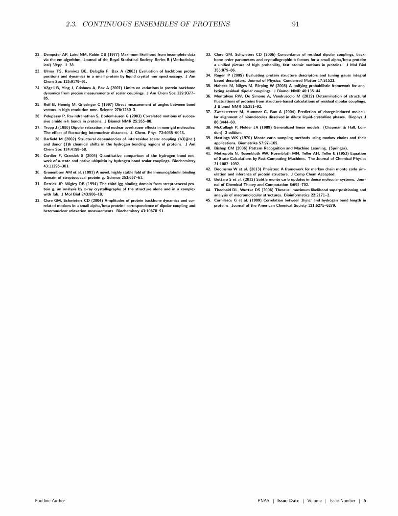
22. Dempster AP, Laird NM, Rubin DB (1977) Maximum likelihood from incomplete data

via the em algorithm. Journal of the Royal Statistical Society. Series B (Methodolog-

ical) 39:pp. 1–38.

23. Ulmer TS, Ramirez BE, Delaglio F, Bax A (2003) Evaluation of backbone proton

positions and dynamics in a small protein by liquid crystal nmr spectroscopy. J Am

Chem Soc 125:9179–91.

24. Vogeli B, Ying J, Grishaev A, Bax A (2007) Limits on variations in protein backbone

dynamics from precise measurements of scalar couplings. J Am Chem Soc 129:9377–

85.

25. Reif B, Hennig M, Griesinger C (1997) Direct measurement of angles between bond

vectors in high-resolution nmr. Science 276:1230–3.

26. Pelupessy P, Ravindranathan S, Bodenhausen G (2003) Correlated motions of succes-

sive amide n-h bonds in proteins. J Biomol NMR 25:265–80.

27. Tropp J (1980) Dipolar relaxation and nuclear overhauser effects in nonrigid molecules:

The effect of fluctuating internuclear distances. J. Chem. Phys. 72:6035–6043.

28. Barfield M (2002) Structural dependencies of interresidue scalar coupling (h3)j(nc’)

and donor (1)h chemical shifts in the hydrogen bonding regions of proteins. J Am

Chem Soc 124:4158–68.

29. Cordier F, Grzesiek S (2004) Quantitative comparison of the hydrogen bond net-

work of a-state and native ubiquitin by hydrogen bond scalar couplings. Biochemistry

43:11295–301.

30. Gronenborn AM et al. (1991) A novel, highly stable fold of the immunoglobulin binding

domain of streptococcal protein g. Science 253:657–61.

31. Derrick JP, Wigley DB (1994) The third igg-binding domain from streptococcal pro-

tein g. an analysis by x-ray crystallography of the structure alone and in a complex

with fab. J Mol Biol 243:906–18.

32. Clore GM, Schwieters CD (2004) Amplitudes of protein backbone dynamics and cor-

related motions in a small alpha/beta protein: correspondence of dipolar coupling and

heteronuclear relaxation measurements. Biochemistry 43:10678–91.

33. Clore GM, Schwieters CD (2006) Concordance of residual dipolar couplings, back-

bone order parameters and crystallographic b-factors for a small alpha/beta protein:

a unified picture of high probability, fast atomic motions in proteins. J Mol Biol

355:879–86.

34. Rogen P (2005) Evaluating protein structure descriptors and tuning gauss integral

based descriptors. Journal of Physics: Condensed Matter 17:S1523.

35. Habeck M, Nilges M, Rieping W (2008) A unifying probabilistic framework for ana-

lyzing residual dipolar couplings. J Biomol NMR 40:135–44.

36. Montalvao RW, De Simone A, Vendruscolo M (2012) Determination of structural

fluctuations of proteins from structure-based calculations of residual dipolar couplings.

J Biomol NMR 53:281–92.

37. Zweckstetter M, Hummer G, Bax A (2004) Prediction of charge-induced molecu-

lar alignment of biomolecules dissolved in dilute liquid-crystalline phases. Biophys J

86:3444–60.

38. McCullagh P, Nelder JA (1989) Generalized linear models. (Chapman & Hall, Lon-

don), 2 edition.

39. Hastings WK (1970) Monte carlo sampling methods using markov chains and their

applications. Biometrika 57:97–109.

40. Bishop CM (2006) Pattern Recognition and Machine Learning. (Springer).

41. Metropolis N, Rosenbluth AW, Rosenbluth MN, Teller AH, Teller E (1953) Equation

of State Calculations by Fast Computing Machines. The Journal of Chemical Physics

21:1087–1092.

42. Boomsma W et al. (2013) Phaistos: A framework for markov chain monte carlo sim-

ulation and inference of protein structure. J Comp Chem Accepted.

43. Bottaro S et al. (2012) Subtle monte carlo updates in dense molecular systems. Jour-

nal of Chemical Theory and Computation 8:695–702.

44. Theobald DL, Wuttke DS (2006) Theseus: maximum likelihood superpositioning and

analysis of macromolecular structures. Bioinformatics 22:2171–2.

45. Cornilescu G et al. (1999) Correlation between 3hjnc‘ and hydrogen bond length in

proteins. Journal of the American Chemical Society 121:6275–6279.



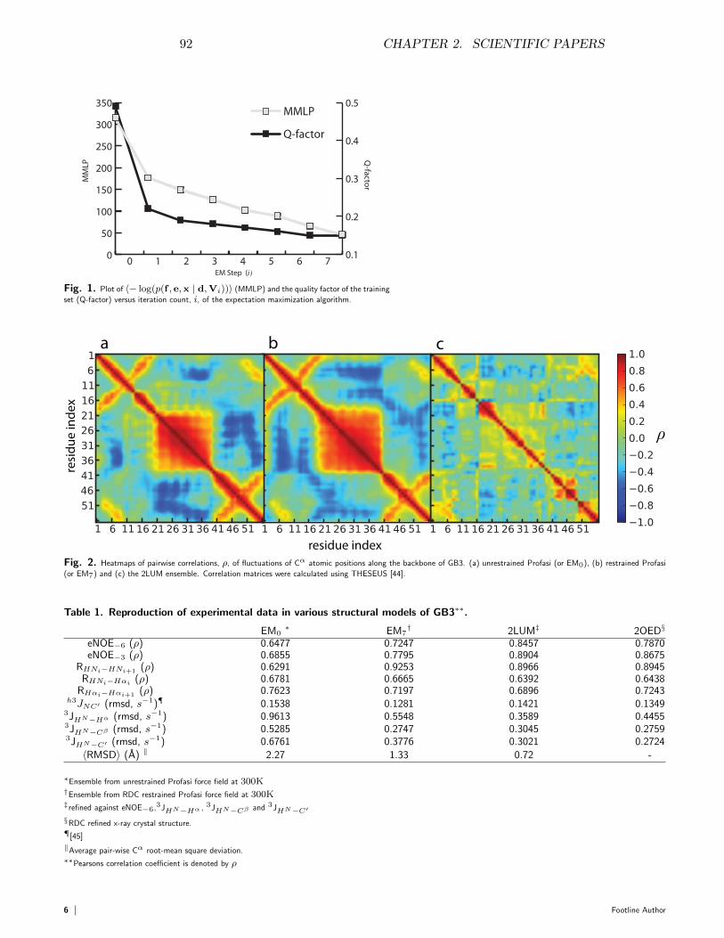
0

50

100

150

200

250

300

350

0.1

0.2

0.3

0.4

0.5MMLP

Q-factor

76543210

MM

LP Q

-facto

r

EM Step (i)

Fig. 1. Plot of 〈− log(p(f , e,x | d,Vi))〉 (MMLP) and the quality factor of the training

set (Q-factor) versus iteration count, i, of the expectation maximization algorithm.

a b c

residue index

resi

du

e in

de

x

ρ

Fig. 2. Heatmaps of pairwise correlations, ρ, of fluctuations of Cα atomic positions along the backbone of GB3. (a) unrestrained Profasi (or EM0), (b) restrained Profasi

(or EM7) and (c) the 2LUM ensemble. Correlation matrices were calculated using THESEUS [44].

Table 1. Reproduction of experimental data in various structural models of GB3∗∗.

EM0∗ EM7

† 2LUM‡ 2OED§

eNOE−6 (ρ) 0.6477 0.7247 0.8457 0.7870eNOE−3 (ρ) 0.6855 0.7795 0.8904 0.8675

RHNi−HNi+1 (ρ) 0.6291 0.9253 0.8966 0.8945RHNi−Hαi (ρ) 0.6781 0.6665 0.6392 0.6438

RHαi−Hαi+1 (ρ) 0.7623 0.7197 0.6896 0.7243h3JNC′ (rmsd, s−1)¶ 0.1538 0.1281 0.1421 0.13493JHN−Hα (rmsd, s−1) 0.9613 0.5548 0.3589 0.44553JHN−Cβ (rmsd, s−1) 0.5285 0.2747 0.3045 0.27593JHN−C′ (rmsd, s−1) 0.6761 0.3776 0.3021 0.2724〈RMSD〉 (A) ‖ 2.27 1.33 0.72 -

∗Ensemble from unrestrained Profasi force field at 300K†Ensemble from RDC restrained Profasi force field at 300K‡refined against eNOE−6,3JHN−Hα , 3JHN−Cβ and 3JHN−C′§RDC refined x-ray crystal structure.¶[45]

‖Average pair-wise Cα root-mean square deviation.∗∗Pearsons correlation coefficient is denoted by ρ

6 Footline Author


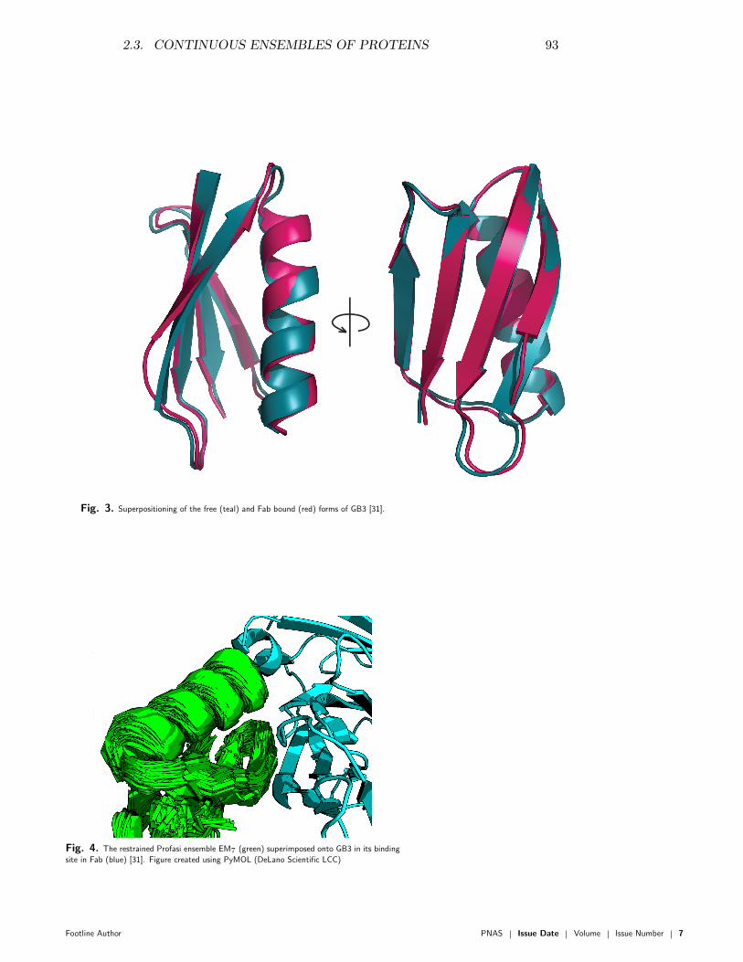
Fig. 3. Superpositioning of the free (teal) and Fab bound (red) forms of GB3 [31].

Fig. 4. The restrained Profasi ensemble EM7 (green) superimposed onto GB3 in its binding

site in Fab (blue) [31]. Figure created using PyMOL (DeLano Scientific LCC)



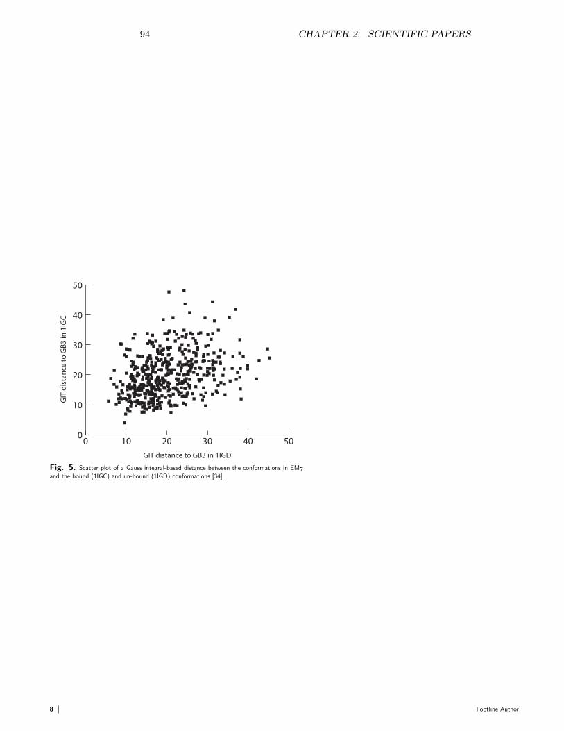
0 10 20 30 40 500

10

20

30

40

50

GIT distance to GB3 in 1IGD

GIT

dis

tan

ce

to

GB

3 i

n 1

IGC

Fig. 5. Scatter plot of a Gauss integral-based distance between the conformations in EM7

and the bound (1IGC) and un-bound (1IGD) conformations [34].

8 Footline Author


Supplementary material for: Construction ofprotein structure ensembles in continuous spacethrough minimal biasing of a simple physical forcefield.Simon Olsson, ∗ and Thomas Hamelryck ∗

∗Bioinformatics Centre, Department of Biology, Faculty of Science, University of Copenhagen, Denmark

draft manuscript

Supplement

Reserved for Publication Footnotes

PNAS Issue Date Volume Issue Number 1–2


Table 1. Cross validation as a function of Expectation Maximization step †.

EM1 EM2 EM3 EM4 EM5 EM6

eNOE−6 (ρ) 0.7093 0.7116 0.7079 0.7262 0.7232 0.7276eNOE−3 (ρ) 0.7527 0.7517 0.7607 0.7792 0.7779 0.7695

RHNi−HNi+1 (ρ) 0.8983 0.9086 0.9179 0.9051 0.9241 0.9263RHNi−Hαi (ρ) 0.6596 0.6677 0.6734 0.6684 0.6759 0.6653

RHαi−Hαi+1 (ρ) 0.7150 0.7212 0.7163 0.7283 0.7221 0.7169h3JNC′ (rmsd, s−1) 0.1393 0.1315 0.1329 0.1309 0.1290 0.1237

3JHN−Hα (rmsd, s−1) 0.6632 0.6242 0.6225 0.5854 0.5226 0.53093JHN−Cβ (rmsd, s−1) 0.3494 0.3275 0.3124 0.3103 0.3021 0.27583JHN−C′ (rmsd, s−1) 0.4652 0.4462 0.4247 0.4194 0.3655 0.3626

〈RMSD〉 (A) ∗ 1.39 1.50 1.46 1.31 1.30 1.42∗Average pair-wise Cα root-mean square deviation.†Pearsons correlation coefficient is denoted by ρ

2 Footline Author


Chapter 3

Closing

3.1 Conclusion and Outlook

The work I have presented in this thesis addresses a central problem instructural biology: How do we construct sensible biomolecular models fromincomplete, noisy and averaged data? – I have approached this questionwith a probabilistic mindset and have found some exciting new methods toachieve this. I will present a summary of the key findings below.

In the first paper, we presented a new implementation of a previouslyreported probabilistic method for protein structure determination, namelyinferential structure determination. We made two conceptual changes tothe original approach. Firstly, we employed more detailed structural priorknowledge embodied in the knowledge-based potentials TorusDBN and Basilisk.Secondly, we employed a different sampling scheme to efficiently traverse theconformational space. We found that the sampling from the posterior dis-tribution converged rapidly compared to what had been reported for theprevious approach. Also, the precision of the obtained structures improved.This was in particular the case for the local structure, due to the prior distri-butions employed. The key result of this study was that inferential structuredetermination had become viable on desktop computers, whereas computerclusters were needed before.

While the inferential structure determination (ISD) approach formallysolves the problem of protein structure determination in a rigorous proba-bilistic framework, it inherently assumes that only a single conformation isreflected in the experimental data. In the second paper, we aimed to general-ize the method to the inference of distributions of protein structures, ratherthan single structures. From first principles we found a hierarchical Bayesiannetwork to be an accurate representation of spatially and temporally aver-

97

98 CHAPTER 3. CLOSING

aged data subject to experimental noise. Importantly, we found ISD consti-tutes an intuitive limit of the model where the ensemble becomes infinitelynarrow. Similarly, we found a recently proposed Maximum Entropy methodfor restraining molecular simulation to also constitute a special case of ourmodel. We found that we were able to reconstruct a high-temperature en-semble of a small hairpin using simulated data subject to both linear andpower averaging. We found the reference distribution to introduce significantbias in the case of power averaged data – this could however be alleviated byusing the reference ratio method. While this study showed great promise onthe proof-of-concept level, it remained unclear whether this method wouldbe tractable in more complex cases.

In the third paper we applied the hierarchical Bayesian model presentedin the second paper in the context of restraining native ensemble simulationswith a physical forcefield. Here, the number of experimental restraints wasmore practically relevant, as was the size of the studied system. We foundthat the restrained ensemble reproduced complementary experimental ev-idence significantly better than the unrestrained simulation. In additionwe found that the fluctuations present in the distribution structures of therestrained ensemble was in agreement with what had previously been pro-posed. Finally, we found a strong concerted motion which had not previouslybeen reported for the free form of the system. These positive results suggeststhat the hierarchical model of averaged data is tractable to more realisticcases.

Discussions of conformational ensembles appear to take up an increasingamount of space on the pages of scientific journals, and rightfully so. How-ever, the inference of single structures from experimental data remains animportant tool, when conformational fluctuations are modest. Still, struc-ture determination from NMR data has been largely limited by the need forexpert assessments with regard to both assignment of resonances to atomsas well as adjustment of empirical parameters in the structure calculationitself. The ISD approach showed immediate promise to alleviate problemsin the latter. In principle it could automatically assess both the quality ofthe data and make a balanced weighing with respect to prior information– this, in a rigorous probabilistic framework. Unfortunately, excessive com-putational demands prohibited most experimental labs from adapting thismethod. Our new implementation will hopefully attract a broader audienceto apply this approach in a more routine fashion – In particular, in caseswhere the approach stands out compared to other methods, e.g. when theavailable experimental evidence is scarce. Future endeavors in this field couldinclude the usage of other more universally accessible data, such as chemical

3.1. CONCLUSION AND OUTLOOK 99

shifts. This has already been reported to be a fruitful direction, outside thecontext of ISD 1 2. We are currently working on a full reimplementationof the presented results into the PHAISTOS framework (see. section 4.3)to be made publicly available. In this connection we are already workingon including chemical shifts into the structure calculation. Furthermore itwould be interesting to experiment with different methods to account forpotential correlations in experimental observables. Both of these endeavorsmay improve the quality and scope of probabilistic structure determinationeven further.

Over the past decades there has been steady progress in structural biol-ogy from considering primarily the singular, rigid structures to understand-ing the structure and its motions – in particular, within the past decade orso, with the emergence of intrinsically disordered proteins as a major classof functional biological molecules. Consequently, the focus on better under-standing disorder, flexibility and dynamics in biological molecules and theirrelation to function has been invigorated 3. From my discussion of methodsto characterize the flexibility of proteins using averaged experimental data itappears that using restrained simulations will be the most sensible endeavor.These provide a framework to bias approximative simulations such that theyagree with experimental data, and may be iteratively refined as more ex-perimental evidence becomes available. More specifically, the restrainingprocedure I presented in the second paper, and other similar approaches 4 5,show great promise as to establish realistic descriptions of the distribution ofbiomolecular structure – see for example the preliminary results in my thirdpaper. Going forward it would be very interesting to apply these methodsto obtain distributions of describing the conformational variability in more

1Andrea Cavalli, Xavier Salvatella,Christopher M. Dobson, and Michele VendruscoloProtein structure determination from NMR chemical shifts (2007) PNAS 104(23)p.9615

2Oliver F. Lange, Paolo Rossi,Nikolaos G. Sgourakis, Yifan Song, Hsiau-Wei Lee, JamesM. Araminic, Asli Ertekin, Rong Xiao, Thomas B. Acton,Gaetano T. Montelione andDavid Baker Determination of solution structures of proteins up to 40 kDausing CS-Rosetta with sparse NMR data from deuterated samples (2012) PNAS109(27) p. 10873

3Kaare Teilum, Johan G. Olsen and Birthe B. Kragelund Protein stability, flexi-bility and function (2011) Biochimica et Biophysica Acta (BBA) - Proteins and Pro-teomics, 1814(8) p.969

4Jed W. Pitera and John D. Chodera On the Use of Experimental Observationsto Bias Simulated Ensembles (2012) JCTC 8(10), p. 3445

5Andrea Cavalli, Carlo Camilloni and Michele Vendruscolo Molecular dynamicssimulations with replica-averaged structural restraints generate structural en-sembles according to the maximum entropy principle (2013) JCP 138(9) p. 094112


dynamic systems such as molten globule or intrinsically disordered proteins.This is something I have already started working on.

3.2. ACKNOWLEDGMENTS 101

3.2 Acknowledgments

Firstly, I’d like to thank my friends and family for their continued supportand encouragements during the work carried out over the past three years.

Secondly, I’d like to thank my supervisor Thomas Hamelryck for invitingme to a PhD in his group and supporting me throughout the process. Third,the rest of the staff and alumni of the Bioinformatics center, in particularWouter Boomsma, Jes Frellsen, Jan Valentin, Lubomir Antonov, Kristof-fer Enøe, Mikael Borg, Christian Andreetta, Tim Harder, Kasper Stovgaardand Martin Paluszewski are thanked. Also to the former DTU group: JesperFerkinghoff-Borg, Sandro Bottaro and Pengfei Tian and SBiN-lab membersMagnus Kjærgaard, Robert Dagil, Kaare Teilum, Kresten Lindorff-Larsenand in particular the late Flemming M. Poulsen, are thanked for their timeand encouraging scientific discussions and great collaborations. Also BeatVogeli at the ETH in Zurich, Switzerland is thanked for interesting discus-sion about NMR and modeling of ensemble data.

Finally, I’d like to thank Douglas L. Theobald and his group a welcomingand stimulating stay at Brandies in july of 2012.

The work carried out in this thesis was funded by a grant from theDanish Council for Independent Research (FTP, 09-066546).

Chapter 4

Appendix

4.1 Appendix A: Technical note on adaptive kernel pro-posals

Given a non-linear function f(x) with x = {xi}Ni=1 the its expected change∂f under a given uncertainty σ(x) is given by the propagation of uncertainty,

∂f =

√√√√n∑

i=1

[∂f

∂xiσ(x)

]2

. (4.1)

When only one parameter, xi, is updated at the time we can without anyloss of generality simplify this to:

∂fi = ‖ ∂f∂xi‖σ(x), (4.2)

where ∂fi corresponds to the expected change in f under the variance σ2

in i. We can now chose a desired change in fi, as ∂fi = ε and isolate anexpression of the standard deviation σ. We obtain,

σ(x) =ε

‖ ∂f∂xi‖. (4.3)

Thus, equation 4.3 yields an optimal choice of standard deviation of ourproposal distribution of a variable xi given a desired change in fi, that is,energy, and the partial derivative of f with respect to that variable. Specialcare must be taken as to assure the change in the proposal distribution isaccounted for in the Metropolis-Hastings criterion.

103

104 CHAPTER 4. APPENDIX

4.2 Appendix B: TYPHON

This paper describes the combination of three advancements made in thegroups of Thomas Hamelryck and Jesper Ferkinghoff-Borg (TorusDBN, Basiliskand CRISP) with a network of Gaussian restraints, to yield a probabilisticequivalent of the popular flexibility predictor tConcoord. In spite of itssimplicity, the model exerts good agreement with experimental data whilekeeping the local structure realistic.This is a co-author article. It was published in Structure in 2012. I wasinvolved in analysis of the results and wrote large parts of the manuscript.

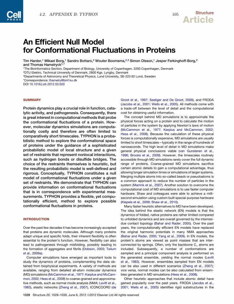
Structure

Article

An Efficient Null Modelfor Conformational Fluctuations in ProteinsTim Harder,1 Mikael Borg,1 Sandro Bottaro,2 Wouter Boomsma,2,3 Simon Olsson,1 Jesper Ferkinghoff-Borg,2

and Thomas Hamelryck1,*1The Bioinformatics Section, Department of Biology, University of Copenhagen, 2200 Copenhagen, Denmark2DTU Elektro, Technical University of Denmark, 2800 Kgs. Lyngby, Denmark3Departments of Astronomy and Theoretical Physics, Lund University, SE-223 62 Lund, Sweden

*Correspondence: [email protected]

DOI 10.1016/j.str.2012.03.020

SUMMARY

Protein dynamics play a crucial role in function, cata-lytic activity, and pathogenesis. Consequently, thereis great interest in computational methods that probethe conformational fluctuations of a protein. How-ever, molecular dynamics simulations are computa-tionally costly and therefore are often limited tocomparatively short timescales. TYPHON is a proba-bilistic method to explore the conformational spaceof proteins under the guidance of a sophisticatedprobabilistic model of local structure and a givenset of restraints that represent nonlocal interactions,such as hydrogen bonds or disulfide bridges. Thechoice of the restraints themselves is heuristic, butthe resulting probabilistic model is well-defined andrigorous. Conceptually, TYPHON constitutes a nullmodel of conformational fluctuations under a givenset of restraints. We demonstrate that TYPHON canprovide information on conformational fluctuationsthat is in correspondence with experimental mea-surements. TYPHON provides a flexible, yet compu-tationally efficient, method to explore possibleconformational fluctuations in proteins.

INTRODUCTION

Over the past few decades it has become increasingly accepted

that proteins are dynamic molecules. Although many proteins

adapt unique and specific folds, their inherent flexibility is often

essential to the protein’s function. However, flexibility can also

lead to pathogenesis through misfolding, possibly leading to

the formation of aggregates and fibrils (Dobson, 2003; Teilum

et al., 2009a).

Computer simulations have emerged as important tools to

study the dynamics of proteins, complementing the data ob-

tained from biophysical experiments. A variety of methods are

available, ranging from detailed all-atom molecular dynamics

(MD) simulations (McCammon et al., 1977; Karplus andMcCam-

mon, 2002; Hess et al., 2008) to coarse-grained and approxima-

tive methods, such as normal mode analysis (NMA; Levitt et al.,

1983), elastic networks (Zheng et al., 2007), tCONCOORD (de

Groot et al., 1997; Seeliger and De Groot, 2009), and FRODA

(Jacobs et al., 2001; Wells et al., 2005). All methods come with

a trade-off between the level of detail and the computational

cost for obtaining useful information.

The concept behind MD simulations is to approximate the

physical forces acting on a protein and to calculate the motion

of particles in the system by applying Newton’s laws of motion

(McCammon et al., 1977; Karplus and McCammon, 2002;

Hess et al., 2008). Because the calculation of these physical

forces is computationally expensive, MD simulations are usually

limited to short timescales—typically in the range of hundreds of

nanoseconds. The high level of detail in MD simulations make

general physical conclusions viable (van Gunsteren et al.,

1996; Brooks et al., 2009). However, the timescales routinely

accessible through MD simulations rarely cover the full dynamic

range of proteins. Coarse-grained MD simulations sacrifice

certain atomic details to gain a computational advantage, thus

allowing longer simulation times or simulations of larger systems.

Merging multiple atoms into so-called beads or pseudoatoms is

a common approach to reduce the number of particles in the

system (Marrink et al., 2007). Another solution to overcome the

computational cost of MD simulations is to use faster computer

hardware. Shaw and colleagues were able to achieve a milli-

second simulation using custom built special-purpose hardware

(Klepeis et al., 2009; Shaw et al., 2010).

Many faster heuristic alternatives toMD have been developed.

The idea behind the elastic network (EN) models is that the

dynamics of folded, native proteins are rather limited compared

to unfolded dynamics and are overall governed by the interresi-

due contact topology (Bahar and Rader, 2005). Over the past

years, the computationally efficient EN models have replaced

the original harmonic potentials in many NMA approaches

(Bahar and Rader, 2005; Yang et al., 2009). In EN models, the

protein’s atoms are viewed as point masses that are inter-

connected by springs. Often, only the backbone Ca atoms are

included. Subsequently, a number of conformations are

sampled and a principal component analysis is performed on

the generated ensemble, yielding the normal modes (Levitt

et al., 1983). However, ensembles sampled from EN models

can be also used in different scenarios (Zheng et al., 2007);

vice versa, normal modes can be also calculated from ensem-

bles generated in MD simulations (Hess et al., 2008).

Other heuristic approaches that include atomic detail have

gained popularity over the past years. FRODA (Jacobs et al.,

2001; Wells et al., 2005) identifies rigid substructures in the

1028 Structure 20, 1028–1039, June 6, 2012 ª2012 Elsevier Ltd All rights reserved

4.2. APPENDIX B: TYPHON 105

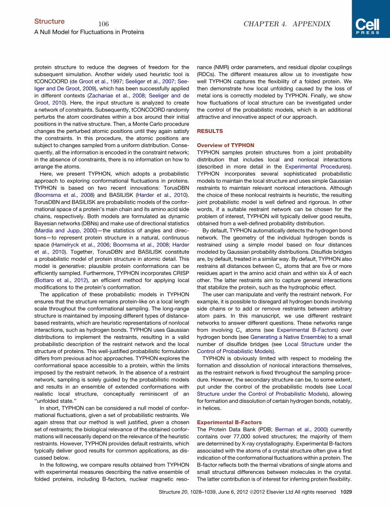
protein structure to reduce the degrees of freedom for the

subsequent simulation. Another widely used heuristic tool is

tCONCOORD (de Groot et al., 1997; Seeliger et al., 2007; See-

liger and De Groot, 2009), which has been successfully applied

in different contexts (Zachariae et al., 2008; Seeliger and de

Groot, 2010). Here, the input structure is analyzed to create

a network of constraints. Subsequently, tCONCOORD randomly

perturbs the atom coordinates within a box around their initial

positions in the native structure. Then, a Monte Carlo procedure

changes the perturbed atomic positions until they again satisfy

the constraints. In this procedure, the atomic positions are

subject to changes sampled from a uniform distribution. Conse-

quently, all the information is encoded in the constraint network;

in the absence of constraints, there is no information on how to

arrange the atoms.

Here, we present TYPHON, which adopts a probabilistic

approach to exploring conformational fluctuations in proteins.

TYPHON is based on two recent innovations: TorusDBN

(Boomsma et al., 2008) and BASILISK (Harder et al., 2010).

TorusDBN and BASILISK are probabilistic models of the confor-

mational space of a protein’s main chain and its amino acid side

chains, respectively. Both models are formulated as dynamic

Bayesian networks (DBNs) and make use of directional statistics

(Mardia and Jupp, 2000)—the statistics of angles and direc-

tions—to represent protein structure in a natural, continuous

space (Hamelryck et al., 2006; Boomsma et al., 2008; Harder

et al., 2010). Together, TorusDBN and BASILISK constitute

a probabilistic model of protein structure in atomic detail. This

model is generative; plausible protein conformations can be

efficiently sampled. Furthermore, TYPHON incorporates CRISP

(Bottaro et al., 2012), an efficient method for applying local

modifications to the protein’s conformation.

The application of these probabilistic models in TYPHON

ensures that the structure remains protein-like on a local length

scale throughout the conformational sampling. The long-range

structure is maintained by imposing different types of distance-

based restraints, which are heuristic representations of nonlocal

interactions, such as hydrogen bonds. TYPHON uses Gaussian

distributions to implement the restraints, resulting in a valid

probabilistic description of the restraint network and the local

structure of proteins. This well-justified probabilistic formulation

differs from previous ad hoc approaches. TYPHON explores the

conformational space accessible to a protein, within the limits

imposed by the restraint network. In the absence of a restraint

network, sampling is solely guided by the probabilistic models

and results in an ensemble of extended conformations with

realistic local structure, conceptually reminiscent of an

‘‘unfolded state.’’

In short, TYPHON can be considered a null model of confor-

mational fluctuations, given a set of probabilistic restraints. We

again stress that our method is well justified, given a chosen

set of restraints; the biological relevance of the obtained confor-

mations will necessarily depend on the relevance of the heuristic

restraints. However, TYPHON provides default restraints, which

typically deliver good results for common applications, as dis-

cussed below.

In the following, we compare results obtained from TYPHON

with experimental measures describing the native ensemble of

folded proteins, including B-factors, nuclear magnetic reso-

nance (NMR) order parameters, and residual dipolar couplings

(RDCs). The different measures allow us to investigate how

well TYPHON captures the flexibility of a folded protein. We

then demonstrate how local unfolding caused by the loss of

metal ions is correctly modeled by TYPHON. Finally, we show

how fluctuations of local structure can be investigated under

the control of the probabilistic models, which is an additional

attractive and innovative aspect of our approach.

RESULTS

Overview of TYPHONTYPHON samples protein structures from a joint probability

distribution that includes local and nonlocal interactions

(described in more detail in the Experimental Procedures).

TYPHON incorporates several sophisticated probabilistic

models to maintain the local structure and uses simple Gaussian

restraints to maintain relevant nonlocal interactions. Although

the choice of these nonlocal restraints is heuristic, the resulting

joint probabilistic model is well defined and rigorous. In other

words, if a suitable restraint network can be chosen for the

problem of interest, TYPHON will typically deliver good results,

obtained from a well-defined probability distribution.

By default, TYPHON automatically detects the hydrogen bond

network. The geometry of the individual hydrogen bonds is

restrained using a simple model based on four distances

modeled by Gaussian probability distributions. Disulfide bridges

are, by default, treated in a similar way. By default, TYPHON also

restrains all distances between Ca atoms that are five or more

residues apart in the amino acid chain and within six A of each

other. The latter restraints aim to capture general interactions

that stabilize the protein, such as the hydrophobic effect.

The user can manipulate and verify the restraint network. For

example, it is possible to disregard all hydrogen bonds involving

side chains or to add or remove restraints between arbitrary

atom pairs. In this manuscript, we use different restraint

networks to answer different questions. These networks range

from involving Ca atoms (see Experimental B-Factors) over

hydrogen bonds (see Generating a Native Ensemble) to a small

number of disulfide bridges (see Local Structure under the

Control of Probabilistic Models).

TYPHON is obviously limited with respect to modeling the

formation and dissolution of nonlocal interactions themselves,

as the restraint network is fixed throughout the sampling proce-

dure. However, the secondary structure can be, to some extent,

put under the control of the probabilistic models (see Local

Structure under the Control of Probabilistic Models), allowing

for formation and dissolution of certain hydrogen bonds, notably,

in helices.

Experimental B-FactorsThe Protein Data Bank (PDB; Berman et al., 2000) currently

contains over 77,000 solved structures; the majority of them

are determined by X-ray crystallography. Experimental B-factors

associated with the atoms of a crystal structure often give a first

indication of the conformational fluctuations within a protein. The

B-factor reflects both the thermal vibrations of single atoms and

small structural differences between molecules in the crystal.

The latter contribution is of interest for inferring protein flexibility.

Structure

A Null Model for Fluctuations in Proteins

Structure 20, 1028–1039, June 6, 2012 ª2012 Elsevier Ltd All rights reserved 1029


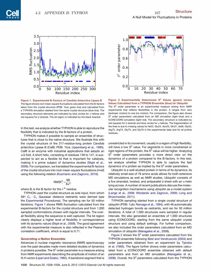
In this test, we analyzewhether TYPHON is able to reproduce the

flexibility that is indicated by the B-factors of a protein.

TYPHON makes it possible to sample an ensemble of struc-

tures that is close to the native structure. We illustrate this with

the crystal structure of the 317-residue-long protein Candida

antarctica Lipase B (CalB; PDB: 1tca; Uppenberg et al., 1995).

CalB is an enzyme with industrial applications that adopts an

a/b fold. A short helix, consisting of residues 139 to 147, is sus-

pected to act as a flexible lid that is important for catalysis,

making it a prime subject of dynamics studies (Skjøt et al.,

2009). For comparison, we translated the experimental B-factors

of the crystal structure into root-mean-square fluctuations (rmsf)

using the following relation (Kuzmanic and Zagrovic, 2010):

RMSF2i =

3Bi

8p2;

where Bi is the B-factor for the i-th residue.

TYPHON used the crystal structure as sole input, from which

581 Ca/Ca Gaussian distance restraints were derived (see

the Experimental Procedures). The sampling ran for 50 million

iterations. Figure 1 shows RMS fluctuation calculated from the

experimental B-factors for the crystal structure and from 1,000

sampled conformations chosen with regular intervals. The over-

all flexibility along the sequence is well captured. The lid region

clearly displays a higher level of flexibility in correspondence

with its dynamic nature (Skjøt et al., 2009). The good agreement

with the experimental measure is also reflected in the Pearson

correlation coefficient, which is equal to 0.71.

Generating a Native EnsembleAdvances in nuclear magnetic resonance (NMR) spectroscopy

over the past decades made more detailed studies of dynamics

in proteins possible. The S2 order parameter is a measure arising

from NMR experiments describing the amplitude of motion of an

N-H vector (Lipari and Szabo, 1982). A backbone segment that is

unrestricted in its movement, usually in a region of high flexibility,

will have a low S2 value. For segments in more constrained or

rigid regions of the protein, the S2 value will be higher. Analyzing

S2 order parameters provides a more direct view on the

dynamics of a protein compared to the B-factors. In this test,

we analyze whether TYPHON is able to capture the fast

dynamics of a protein as implied by the S2 order parameters.

Ubiquitin is a well-studied protein in terms of its dynamics; its

relatively small size of 76 amino acids allows for both extensive

MD simulations as well as NMR studies. Ubiquitin consists of

a five stranded, twisted, and antiparallel b sheet with an a-helix

lying across. A number of recent publications discuss themolec-

ular recognition mechanisms using ubiquitin as a model system

(Lange et al., 2008; Wlodarski and Zagrovic, 2009; Long and

Bruschweiler, 2011).

TYPHON sampling started from a single crystal structure of

ubiquitin (PDB: 1ubi; Ramage et al., 1994), with 46 automatically

detected hydrogen bonds as restraints, and ran for 50 million

iterations. A total of 1,000 structures were sampled in regular

intervals. We also generated an ensemble of 1,000 structures

using tCONCOORD, starting from the same ubiquitin crystal

structure and using default settings. For further comparison,

we also included the order parameters calculated from an MD

simulation of ubiquitin (Maragakis et al., 2008).

Figure 2 shows the S2 order parameters calculated from the

TYPHON ensemble following Best and Vendruscolo (2004) and

order parameters obtained from an experiment by Tjandra

et al. (1995). The figure further shows order parameters calcu-

lated from a tCONCOORD ensemble obtained with default

parameters and from an MD simulation (Maragakis et al.,

2008). Overall, the S2 parameters calculated from the TYPHON

Figure 1. Experimental B-Factors of Candida Antarctica Lipase B

The figure shows root-mean-square fluctuations calculated from the B-factors

taken from the crystal structure (PDB: 1tca; green line) and calculated from

a TYPHON simulation started from the same crystal structure (blue line). The

secondary structure elements are indicated by blue circles for a helices and

red squares for b strands. The lid region is indicated by the black bracket.

Figure 2. Experimentally Determined S2 Values (green) versus

Values Calculated from a TYPHON Ensemble (blue) for UbiquitinThe S2 order parameter is an experimental measure arising from NMR

experiments that reflects flexibilities in the protein. It ranges from zero

(isotropic motion) to one (no motion). For comparison, the figure also shows

S2 order parameters calculated from an MD simulation (light blue) and a

tCONCOORD simulation (light red). The secondary structure is indicated by

red squares for b strands and blue circles for a helices. The fragmentation of

the lines is due to missing values for Ile23, Glu24, Asn25, Gln31, Ile36, Gly53,

Arg72, Arg74, Gly75, and Gly76 in the experimental data and for all proline

residues.

Structure




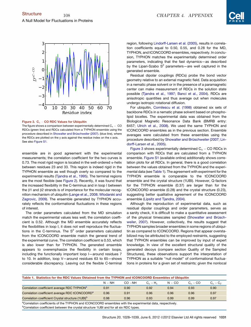
ensemble are in good agreement with the experimental

measurements; the correlation coefficient for the two curves is

0.73. The most rigid region is located in the well-ordered a-helix

between residues 23 and 33. This region is indeed rigid in the

TYPHON ensemble as well though overly so compared to the

experimental results (Tjandra et al., 1995). The terminal regions

are the most flexible (see Figure 2). Recently, it was found that

the increased flexibility in the C-terminus and in loop I between

the b1 and b2 strands is of importance for the molecular recog-

nition mechanism of ubiquitin (Lange et al., 2008; Wlodarski and

Zagrovic, 2009). The ensemble generated by TYPHON accu-

rately reflects the conformational fluctuations in these regions

of interest.

The order parameters calculated from the MD simulation

match the experimental values less well; the correlation coeffi-

cient is 0.52. Although the MD ensemble accurately reflects

the flexibilities in loop I, it does not well reproduce the fluctua-

tions in the C-terminus. The S2 order parameters calculated

from the tCONCOORD ensemble match the general trend of

the experimental curve. The correlation coefficient is 0.53, which

is also lower than for TYPHON. The generated ensemble

appears to overemphasize the flexibility in certain loops,

including the functionally important loop I—around residues 7

to 10. In addition, loop V—around residues 63 to 65—shows

considerable discrepancy. Leaving out the flexible C-terminal

region, following Lindorff-Larsen et al. (2005), results in correla-

tion coefficients equal to 0.50, 0.55, and 0.28 for the MD,

TYPHON, and tCONCOORD ensembles, respectively. In conclu-

sion, TYPHON matches the experimentally determined order

parameters, indicating that the fast dynamics—as described

by the Lipari-Szabo S2 parameters—are well captured in the

generated ensemble.

Residual dipolar couplings (RDCs) probe the bond vector

geometry relative to an external magnetic field. Data acquisition

in a nematic phase solvent or in the presence of a paramagnetic

center can make measurement of RDCs in the solution state

possible (Tjandra et al., 1997; Banci et al., 2004). RDCs are

anisotropic quantities and thus average out when molecules

undergo isotropic rotational diffusion.

For ubiquitin, Cornilescu et al. (1998) obtained six sets of

backbone RDCs in a nematic phase solvent based on phospho-

lipid bicelles. The experimental data was obtained from the

Biological Magnetic Resonance Data Bank (BMRB entry:

6457; Ulrich et al., 2008). We used the same TYPHON and

tCONCOORD ensembles as in the previous section. Ensemble

averages were calculated from these ensembles using the

procedure described by Showalter and Bruschweiler (2007; Lin-

dorff-Larsen et al., 2005).

Figure 3 shows experimentally determined Ca � CO RDCs in

comparison with RDCs that are calculated from a TYPHON

ensemble. Figure S1 (available online) additionally shows corre-

lation plots for all RDCs. In general, there is a good correlation

between the values obtained from the TYPHON and the experi-

mental data (see Table 1). The agreement with experiment for the

TYPHON ensemble is comparable to the tCONCOORD

ensemble and the crystal structure (1UBI). However, Q-factors

for the TYPHON ensemble (0.37) are larger than for the

tCONCOORD ensemble (0.28) and the crystal structure (0.23),

suggesting better qualitative agreement of the tCONCOORD

ensemble (Lipsitz and Tjandra, 2004).

Although the reproduction of experimental data, such as

residual dipolar couplings and order parameters, serves as

a sanity check, it is difficult to make a quantitative assessment

of the physical timescales sampled (Showalter and Brusch-

weiler, 2007). However, collectively, the results suggest that

TYPHON samples broader ensembles in some regions of ubiqui-

tin as compared to tCONCOORD. Regions that appear oversta-

bilized may be attributed to the employed restraints, suggesting

that TYPHON ensembles can be improved by input of expert

knowledge. In view of the excellent structural quality of the

generated decoys (compare section Quality of the Sampled

Structures), these observations support the interpretation of

TYPHON as a suitable ‘‘null model’’ of conformational fluctua-

tions in proteins for a given set of restraints; given the nonlocal

Figure 3. Ca � CO RDC Values for Ubiquitin

The figure shows a comparison between experimentally determined Ca � CO

RDCs (green line) and RDCs calculated from a TYPHON ensemble using the

procedure described in Showalter and Bruschweiler (2007). (blue line), where

the RDCs are plotted on the y axis against the residue index on the x axis.

See also Figure S1.

Table 1. Statistics for the RDC Values Obtained from the TYPHON and tCONCOORD Ensembles of Ubiquitin

N � NH CO �NH Ca � Ha N � CO Ca � CO Ca � Cb

Correlation coefficient average RDC TYPHONa 0.91 0.90 0.92 0.94 0.93 0.90

Correlation coefficient average RDC tCONCOORDa 0.96 0.91 0.96 0.96 0.96 0.97

Correlation coefficient Crystal structure (1UBI)b 0.98 0.96 0.93 0.99 0.99 0.97aCorrelation coefficients of the TYPHON and tCONCOORD ensembles with the experimental data, respectively.bCorrelation coefficient between the crystal structure 1UBI and for all six RDC types.

Structure




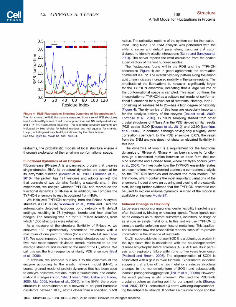
restraints, the probabilistic models of local structure ensure a

thorough exploration of the remaining conformational space.

Functional Dynamics of an EnzymeRibonuclease (RNase) A is a pancreatic protein that cleaves

single-stranded RNA; its structural dynamics are essential for

its enzymatic function (Doucet et al., 2009; Formoso et al.,

2010). The protein has 124 residues and adopts an a/b fold

that consists of two domains flanking a catalytic site. In this

experiment, we analyze whether TYPHON can reproduce the

functional dynamics of RNase A. In addition, we compare the

TYPHON ensemble to results obtained from NMA.

We initialized TYPHON sampling from the RNase A crystal

structure (PDB: 7RSA; Wlodawer et al., 1988) and used the

automatically detected hydrogen bond network with default

settings, resulting in 76 hydrogen bonds and four disulfide

bridges. The sampling was run for 100 million iterations, from

which 1,000 structures were retained.

As a measure of the structural flexibility of RNase A, we

analyzed 132 experimentally determined structures with a

maximum of one point mutation (for a complete list see Table

S1). We superimposed the experimental structures using itera-

tive root-mean-square deviation (rmsd) minimization to the

average structure and calculated the rmsf of the Ca atoms. We

call this set the high-sequence similarity PDB ensemble (Best

et al., 2006).

In addition, we compare our result to the dynamics of the

enzyme according to the elastic network model (ENM), a

coarse-grained model of protein dynamics that has been used

to analyze collective motions, residue fluctuations, and confor-

mational changes (Tirion, 1996; Hinsen, 1998; Bahar and Rader,

2005; Ma, 2005; Kimber et al., 2010). In the ENM, the protein

structure is approximated as a network of coupled harmonic

oscillators between all Ca atoms closer than a specified cutoff

radius. The collective motions of the system can be then calcu-

lated using NMA. The ENM analysis was performed with the

elNemo server and default parameters, using an 8 A cutoff

distance to identify elastic interactions (Suhre and Sanejouand,

2004). The server reports the rmsf calculated from the scaled

Eigen vectors of the first hundred modes.

The fluctuations found within the PDB and the TYPHON

ensembles (Figure 4) are in good agreement; the correlation

coefficient is 0.72. The overall flexibility pattern along the amino

acid chain indicates increased mobility in the same regions. The

amplitude of the fluctuations is, however, significantly larger

for the TYPHON ensemble, indicating that a large volume of

the conformational space is sampled. This again confirms the

interpretation of TYPHON as a suitable null model of conforma-

tional fluctuations for a given set of restraints. Notably, loop I—

consisting of residues 14 to 25—has a high degree of flexibility

(Figure 4). The dynamics of this loop are especially important

for the catalytic activity of the enzyme (Doucet et al., 2009;

Formoso et al., 2010). TYPHON sampling started from other

crystal structures of RNase A in the PDB yielded similar results

(PDB codes 3LXO [Doucet et al., 2010] and 2G8Q [Leonidas

et al., 2006]). In contrast, although having only a slightly lower

correlation coefficient to the PDB ensemble (0.67), the result

from the ENM analysis does not show an elevated flexibility in

this loop.

The dynamics of loop I is a requirement for the functional

dynamics of RNase A; RNase A has been shown to function

through a concerted motion between an open form that can

bind substrate and a closed form, where catalysis occurs (Watt

et al., 2007). To investigate how the TYPHON ensemble relates

to these motions, we performed a principle component analysis

on the TYPHON samples and isolated the main modes. The

first mode, which contains the most important variations of the

ensemble, indeed shows an opening and closing of the catalytic

cleft, lending further evidence that the TYPHON ensemble can

be used to explore enzyme dynamics. A video of the motion is

available online (see Movie S1).

Induced Change in FlexibilityLarge-scalemotions ormajor changes in flexibility in proteins are

often induced by binding or releasing ligands. These ligands can

be as complex as multiatom substrates, inhibitors, or drugs or

as simple as single metal ions. In this test we use TYPHON to

simulate partial unfolding upon loss of metal ions. This applica-

tion illustrates how the probabilistic models ‘‘step in’’ to provide

information in the absence of restraints.

Cu/Zn superoxide dismutase (SOD1) is a ubiquitous protein in

the cytoplasm that is associated with the neurodegenerative

disease amyotrophic lateral sclerosis (ALS). ALS results in paral-

ysis and respiratory failure within one to five years from onset

(Pasinelli and Brown, 2006). The oligomerization of SOD1 is

associated with a gain in toxic function. Experimental evidence

suggests that a loss of the two metal ions induces structural

changes to the monomeric form of SOD1 and subsequently

leads to pathogenic aggregation (Teilum et al., 2009b). However,

the exact pathway is still unknown. We used the PDB:2v0a

crystal structure as starting point for our experiments (Strange

et al., 2007). SOD1 consists of a b barrel with long loops connect-

ing the antiparallel strands. It contains a disulfide bridge and has

Figure 4. RMS Fluctuations Showing Dynamics of Ribonuclease AThe plot shows the RMS fluctuations measured from a set of PDB structures

(see Functional Dynamics of an Enzyme, green line), an ENManalysis (red line),

and a TYPHON simulation (blue line). The secondary structure elements are

indicated by blue circles for helical residues and red squares for strands.

Loop I, including residues 14–25, is indicated by the black bracket.

See also Figure S2, Movie S1, and Table S1.

Structure




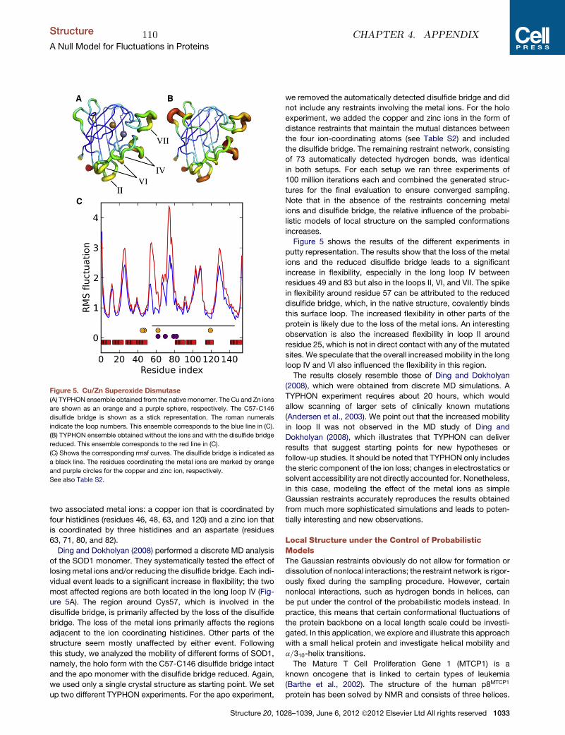
two associated metal ions: a copper ion that is coordinated by

four histidines (residues 46, 48, 63, and 120) and a zinc ion that

is coordinated by three histidines and an aspartate (residues

63, 71, 80, and 82).

Ding and Dokholyan (2008) performed a discrete MD analysis

of the SOD1 monomer. They systematically tested the effect of

losing metal ions and/or reducing the disulfide bridge. Each indi-

vidual event leads to a significant increase in flexibility; the two

most affected regions are both located in the long loop IV (Fig-

ure 5A). The region around Cys57, which is involved in the

disulfide bridge, is primarily affected by the loss of the disulfide

bridge. The loss of the metal ions primarily affects the regions

adjacent to the ion coordinating histidines. Other parts of the

structure seem mostly unaffected by either event. Following

this study, we analyzed the mobility of different forms of SOD1,

namely, the holo form with the C57-C146 disulfide bridge intact

and the apo monomer with the disulfide bridge reduced. Again,

we used only a single crystal structure as starting point. We set

up two different TYPHON experiments. For the apo experiment,

we removed the automatically detected disulfide bridge and did

not include any restraints involving the metal ions. For the holo

experiment, we added the copper and zinc ions in the form of

distance restraints that maintain the mutual distances between

the four ion-coordinating atoms (see Table S2) and included

the disulfide bridge. The remaining restraint network, consisting

of 73 automatically detected hydrogen bonds, was identical

in both setups. For each setup we ran three experiments of

100 million iterations each and combined the generated struc-

tures for the final evaluation to ensure converged sampling.

Note that in the absence of the restraints concerning metal

ions and disulfide bridge, the relative influence of the probabi-

listic models of local structure on the sampled conformations

increases.

Figure 5 shows the results of the different experiments in

putty representation. The results show that the loss of the metal

ions and the reduced disulfide bridge leads to a significant

increase in flexibility, especially in the long loop IV between

residues 49 and 83 but also in the loops II, VI, and VII. The spike

in flexibility around residue 57 can be attributed to the reduced

disulfide bridge, which, in the native structure, covalently binds

this surface loop. The increased flexibility in other parts of the

protein is likely due to the loss of the metal ions. An interesting

observation is also the increased flexibility in loop II around

residue 25, which is not in direct contact with any of the mutated

sites. We speculate that the overall increased mobility in the long

loop IV and VI also influenced the flexibility in this region.

The results closely resemble those of Ding and Dokholyan

(2008), which were obtained from discrete MD simulations. A

TYPHON experiment requires about 20 hours, which would

allow scanning of larger sets of clinically known mutations

(Andersen et al., 2003). We point out that the increased mobility

in loop II was not observed in the MD study of Ding and

Dokholyan (2008), which illustrates that TYPHON can deliver

results that suggest starting points for new hypotheses or

follow-up studies. It should be noted that TYPHON only includes

the steric component of the ion loss; changes in electrostatics or

solvent accessibility are not directly accounted for. Nonetheless,

in this case, modeling the effect of the metal ions as simple

Gaussian restraints accurately reproduces the results obtained

from much more sophisticated simulations and leads to poten-

tially interesting and new observations.

Local Structure under the Control of ProbabilisticModelsThe Gaussian restraints obviously do not allow for formation or

dissolution of nonlocal interactions; the restraint network is rigor-

ously fixed during the sampling procedure. However, certain

nonlocal interactions, such as hydrogen bonds in helices, can

be put under the control of the probabilistic models instead. In

practice, this means that certain conformational fluctuations of

the protein backbone on a local length scale could be investi-

gated. In this application, we explore and illustrate this approach

with a small helical protein and investigate helical mobility and

a=310-helix transitions.

The Mature T Cell Proliferation Gene 1 (MTCP1) is a

known oncogene that is linked to certain types of leukemia

(Barthe et al., 2002). The structure of the human p8MTCP1

protein has been solved by NMR and consists of three helices.

Figure 5. Cu/Zn Superoxide Dismutase

(A) TYPHON ensemble obtained from the native monomer. The Cu and Zn ions

are shown as an orange and a purple sphere, respectively. The C57-C146

disulfide bridge is shown as a stick representation. The roman numerals

indicate the loop numbers. This ensemble corresponds to the blue line in (C).

(B) TYPHON ensemble obtained without the ions and with the disulfide bridge

reduced. This ensemble corresponds to the red line in (C).

(C) Shows the corresponding rmsf curves. The disulfide bridge is indicated as

a black line. The residues coordinating the metal ions are marked by orange

and purple circles for the copper and zinc ion, respectively.

See also Table S2.

Structure




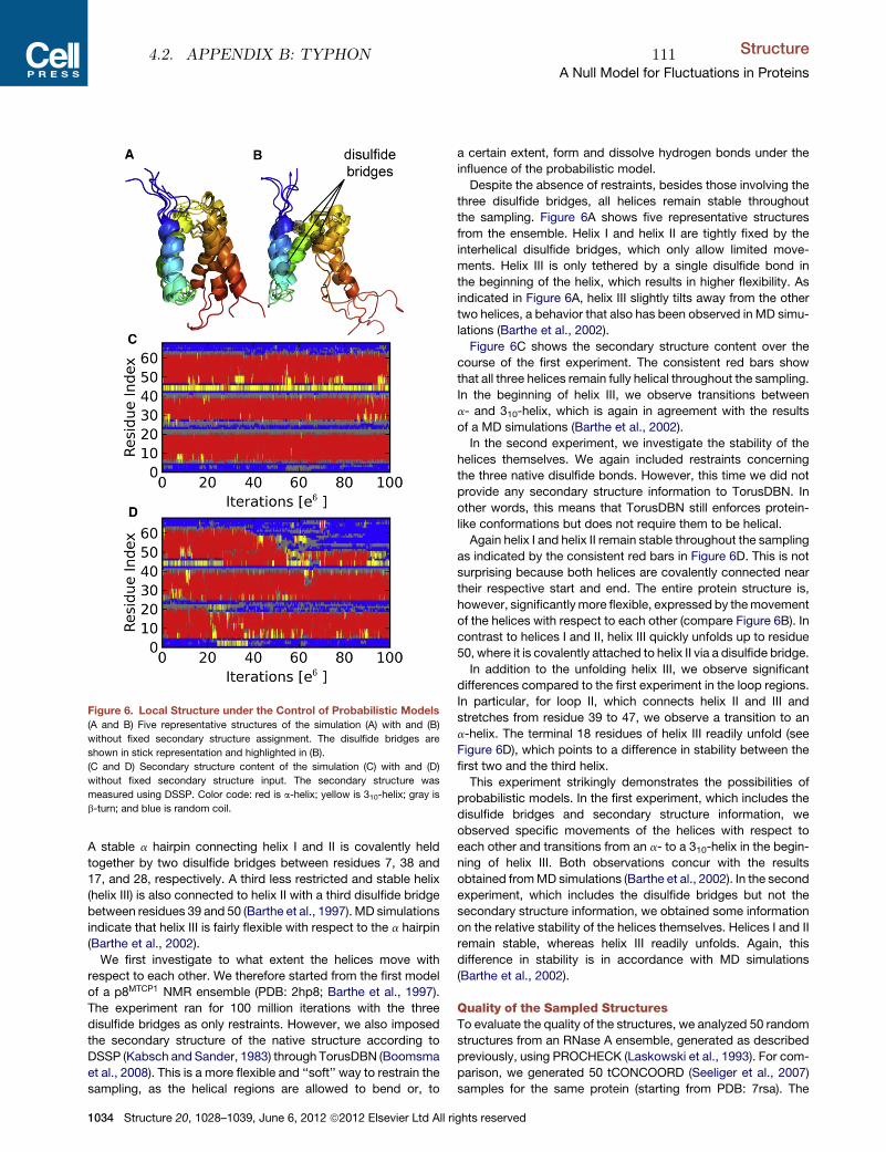
A stable a hairpin connecting helix I and II is covalently held

together by two disulfide bridges between residues 7, 38 and

17, and 28, respectively. A third less restricted and stable helix

(helix III) is also connected to helix II with a third disulfide bridge

between residues 39 and 50 (Barthe et al., 1997). MD simulations

indicate that helix III is fairly flexible with respect to the a hairpin

(Barthe et al., 2002).

We first investigate to what extent the helices move with

respect to each other. We therefore started from the first model

of a p8MTCP1 NMR ensemble (PDB: 2hp8; Barthe et al., 1997).

The experiment ran for 100 million iterations with the three

disulfide bridges as only restraints. However, we also imposed

the secondary structure of the native structure according to

DSSP (Kabsch and Sander, 1983) through TorusDBN (Boomsma

et al., 2008). This is a more flexible and ‘‘soft’’ way to restrain the

sampling, as the helical regions are allowed to bend or, to

a certain extent, form and dissolve hydrogen bonds under the

influence of the probabilistic model.

Despite the absence of restraints, besides those involving the

three disulfide bridges, all helices remain stable throughout

the sampling. Figure 6A shows five representative structures

from the ensemble. Helix I and helix II are tightly fixed by the

interhelical disulfide bridges, which only allow limited move-

ments. Helix III is only tethered by a single disulfide bond in

the beginning of the helix, which results in higher flexibility. As

indicated in Figure 6A, helix III slightly tilts away from the other

two helices, a behavior that also has been observed in MD simu-

lations (Barthe et al., 2002).

Figure 6C shows the secondary structure content over the

course of the first experiment. The consistent red bars show

that all three helices remain fully helical throughout the sampling.

In the beginning of helix III, we observe transitions between

a- and 310-helix, which is again in agreement with the results

of a MD simulations (Barthe et al., 2002).

In the second experiment, we investigate the stability of the

helices themselves. We again included restraints concerning

the three native disulfide bonds. However, this time we did not

provide any secondary structure information to TorusDBN. In

other words, this means that TorusDBN still enforces protein-

like conformations but does not require them to be helical.

Again helix I and helix II remain stable throughout the sampling

as indicated by the consistent red bars in Figure 6D. This is not

surprising because both helices are covalently connected near

their respective start and end. The entire protein structure is,

however, significantlymore flexible, expressed by themovement

of the helices with respect to each other (compare Figure 6B). In

contrast to helices I and II, helix III quickly unfolds up to residue

50, where it is covalently attached to helix II via a disulfide bridge.

In addition to the unfolding helix III, we observe significant

differences compared to the first experiment in the loop regions.

In particular, for loop II, which connects helix II and III and

stretches from residue 39 to 47, we observe a transition to an

a-helix. The terminal 18 residues of helix III readily unfold (see

Figure 6D), which points to a difference in stability between the

first two and the third helix.

This experiment strikingly demonstrates the possibilities of

probabilistic models. In the first experiment, which includes the

disulfide bridges and secondary structure information, we

observed specific movements of the helices with respect to

each other and transitions from an a- to a 310-helix in the begin-

ning of helix III. Both observations concur with the results

obtained fromMD simulations (Barthe et al., 2002). In the second

experiment, which includes the disulfide bridges but not the

secondary structure information, we obtained some information

on the relative stability of the helices themselves. Helices I and II

remain stable, whereas helix III readily unfolds. Again, this

difference in stability is in accordance with MD simulations

(Barthe et al., 2002).

Quality of the Sampled StructuresTo evaluate the quality of the structures, we analyzed 50 random

structures from an RNase A ensemble, generated as described

previously, using PROCHECK (Laskowski et al., 1993). For com-

parison, we generated 50 tCONCOORD (Seeliger et al., 2007)

samples for the same protein (starting from PDB: 7rsa). The

Figure 6. Local Structure under the Control of Probabilistic Models

(A and B) Five representative structures of the simulation (A) with and (B)

without fixed secondary structure assignment. The disulfide bridges are

shown in stick representation and highlighted in (B).

(C and D) Secondary structure content of the simulation (C) with and (D)

without fixed secondary structure input. The secondary structure was

measured using DSSP. Color code: red is a-helix; yellow is 310-helix; gray is

b-turn; and blue is random coil.

Structure




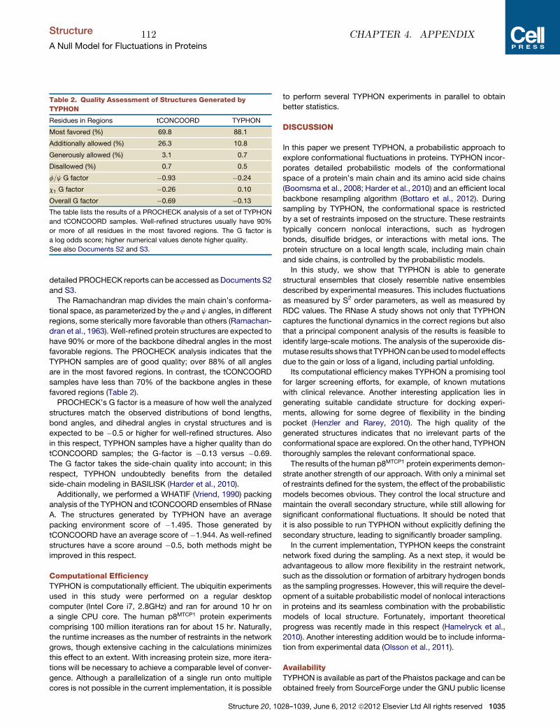
detailed PROCHECK reports can be accessed as Documents S2

and S3.

The Ramachandran map divides the main chain’s conforma-

tional space, as parameterized by the 4 and j angles, in different

regions, some sterically more favorable than others (Ramachan-

dran et al., 1963). Well-refined protein structures are expected to

have 90% or more of the backbone dihedral angles in the most

favorable regions. The PROCHECK analysis indicates that the

TYPHON samples are of good quality; over 88% of all angles

are in the most favored regions. In contrast, the tCONCOORD

samples have less than 70% of the backbone angles in these

favored regions (Table 2).

PROCHECK’s G factor is a measure of how well the analyzed

structures match the observed distributions of bond lengths,

bond angles, and dihedral angles in crystal structures and is

expected to be �0.5 or higher for well-refined structures. Also

in this respect, TYPHON samples have a higher quality than do

tCONCOORD samples; the G-factor is �0.13 versus �0.69.The G factor takes the side-chain quality into account; in this

respect, TYPHON undoubtedly benefits from the detailed

side-chain modeling in BASILISK (Harder et al., 2010).

Additionally, we performed a WHATIF (Vriend, 1990) packing

analysis of the TYPHON and tCONCOORD ensembles of RNase

A. The structures generated by TYPHON have an average

packing environment score of �1.495. Those generated by

tCONCOORD have an average score of �1.944. As well-refined

structures have a score around �0.5, both methods might be

improved in this respect.

Computational EfficiencyTYPHON is computationally efficient. The ubiquitin experiments

used in this study were performed on a regular desktop

computer (Intel Core i7, 2.8GHz) and ran for around 10 hr on

a single CPU core. The human p8MTCP1 protein experiments

comprising 100 million iterations ran for about 15 hr. Naturally,

the runtime increases as the number of restraints in the network

grows, though extensive caching in the calculations minimizes

this effect to an extent. With increasing protein size, more itera-

tions will be necessary to achieve a comparable level of conver-

gence. Although a parallelization of a single run onto multiple

cores is not possible in the current implementation, it is possible

to perform several TYPHON experiments in parallel to obtain

better statistics.

DISCUSSION

In this paper we present TYPHON, a probabilistic approach to

explore conformational fluctuations in proteins. TYPHON incor-

porates detailed probabilistic models of the conformational

space of a protein’s main chain and its amino acid side chains

(Boomsma et al., 2008; Harder et al., 2010) and an efficient local

backbone resampling algorithm (Bottaro et al., 2012). During

sampling by TYPHON, the conformational space is restricted

by a set of restraints imposed on the structure. These restraints

typically concern nonlocal interactions, such as hydrogen

bonds, disulfide bridges, or interactions with metal ions. The

protein structure on a local length scale, including main chain

and side chains, is controlled by the probabilistic models.

In this study, we show that TYPHON is able to generate

structural ensembles that closely resemble native ensembles

described by experimental measures. This includes fluctuations

as measured by S2 order parameters, as well as measured by

RDC values. The RNase A study shows not only that TYPHON

captures the functional dynamics in the correct regions but also

that a principal component analysis of the results is feasible to

identify large-scale motions. The analysis of the superoxide dis-

mutase results shows that TYPHONcanbeused tomodel effects

due to the gain or loss of a ligand, including partial unfolding.

Its computational efficiency makes TYPHON a promising tool

for larger screening efforts, for example, of known mutations

with clinical relevance. Another interesting application lies in

generating suitable candidate structure for docking experi-

ments, allowing for some degree of flexibility in the binding

pocket (Henzler and Rarey, 2010). The high quality of the

generated structures indicates that no irrelevant parts of the

conformational space are explored. On the other hand, TYPHON

thoroughly samples the relevant conformational space.

The results of the human p8MTCP1 protein experiments demon-

strate another strength of our approach. With only a minimal set

of restraints defined for the system, the effect of the probabilistic

models becomes obvious. They control the local structure and

maintain the overall secondary structure, while still allowing for

significant conformational fluctuations. It should be noted that

it is also possible to run TYPHON without explicitly defining the

secondary structure, leading to significantly broader sampling.

In the current implementation, TYPHON keeps the constraint

network fixed during the sampling. As a next step, it would be

advantageous to allow more flexibility in the restraint network,

such as the dissolution or formation of arbitrary hydrogen bonds

as the sampling progresses. However, this will require the devel-

opment of a suitable probabilistic model of nonlocal interactions

in proteins and its seamless combination with the probabilistic

models of local structure. Fortunately, important theoretical

progress was recently made in this respect (Hamelryck et al.,

2010). Another interesting addition would be to include informa-

tion from experimental data (Olsson et al., 2011).

AvailabilityTYPHON is available as part of the Phaistos package and can be

obtained freely from SourceForge under the GNU public license

Table 2. Quality Assessment of Structures Generated by

TYPHON

Residues in Regions tCONCOORD TYPHON

Most favored (%) 69.8 88.1

Additionally allowed (%) 26.3 10.8

Generously allowed (%) 3.1 0.7

Disallowed (%) 0.7 0.5

f=j G factor �0.93 �0.24c1 G factor �0.26 0.10

Overall G factor �0.69 �0.13The table lists the results of a PROCHECK analysis of a set of TYPHON

and tCONCOORD samples. Well-refined structures usually have 90%

or more of all residues in the most favored regions. The G factor is

a log odds score; higher numerical values denote higher quality.

See also Documents S2 and S3.

Structure




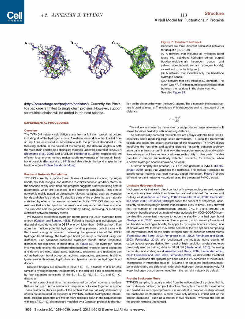
(http://sourceforge.net/projects/phaistos/). Currently the Phais-

tos package is limited to single chain proteins. However, support

for multiple chains will be added in the next release.

EXPERIMENTAL PROCEDURES

Overview

The TYPHON network calculation starts from a full atom protein structure,

including all of the hydrogen atoms. A restraint network is either loaded from

an input file or created in accordance with the protocol described in the

following section. In the course of the sampling, the dihedral angles in both

themain chain and the side chains aremodified under the control of TorusDBN

(Boomsma et al., 2008) and BASILISK (Harder et al., 2010), respectively. An

efficient local moves method makes subtle movements of the protein back-

bone possible (Bottaro et al., 2012) and also affects the bond angles in the

backbone (see Protein Backbone Move).

Restraint Network Calculation

TYPHON currently supports three classes of restraints involving hydrogen

bonds, disulfide bridges, and distance restraints between arbitrary atoms. In

the absence of any user input, the program suggests a network using default

parameters, which are described in the following paragraphs. This default

network is mainly based on biologically relevant restraints, such as hydrogen

bonds and disulfide bridges. To stabilize parts of the protein that are naturally

stabilized by effects that are not modeled explicitly, TYPHON also connects

residues that are far apart in the amino acid sequence but close in space.

The user can edit the generated network by adding, removing, or modifying

restraints between arbitrary atoms.

We evaluate all potential hydrogen bonds using the DSSP hydrogen bond

energy (Kabsch and Sander, 1983). Following Kabsch and colleagues, we

discard all candidates with a DSSP energy higher than �0:5ðkcal=molÞ. If anatom has multiple potential hydrogen bonding partners, only the one with

the lowest energy is retained. Following the general idea of the DSSP

hydrogen bond energy, the hydrogen bond geometry is modeled using four

distances. For backbone-backbone hydrogen bonds, these respective

distances are explained in more detail in Figure S3. For hydrogen bonds

involving side chains, the corresponding standard hydrogen bond acceptors

and donors are used; asparagine, aspartate, glutamine, and glutamate can

act as hydrogen bond acceptors; arginine, asparagine, glutamine, histidine,

lysine, serine, threonine, tryptophan, and tyrosine can act as hydrogen bond

donors.

Disulfide bridges are required to have a Sg/Sg distance of 3 A or less.

Similar to hydrogen bonds, the geometry of the disulfide bond is also modeled

by four distances consisting of the Sg/Sg, Cb/Sg, Sg/Cb, and Cb/Cb

distances.

The last class of restraints that are detected by default connects residues

that are far apart in the amino acid sequence but close together in space.

These restraints stabilize parts of the protein that are naturally stabilized by

effects not accounted for explicitly in TYPHON, such as hydrophobic interac-

tions. Residue pairs that are five or more residues apart in the sequence but

within six A (Ca/Ca distance) are modeled by a Gaussian probability distribu-

tion on the distance between the twoCa atoms. The distance in the input struc-

ture is used as mean m. The variance s2 is set proportional to the square of the

distance:

s2 =�m6

�2

:

This value was chosen by trial-and-error and produces reasonable results. It

allows for more flexibility with increasing distance.

The automatically detected restraints will not always yield the best results,

especially when modeling large-scale movements. To keep the framework

flexible and utilize the expert knowledge of the researcher, TYPHON allows

modifying the restraints and adding distance restraints between arbitrary

atom pairs in the structure. In that way, the researcher may additionally stabi-

lize certain parts of the structure or allowmore flexibility in other parts. It is also

possible to remove automatically detected restraints, for example, when

a certain hydrogen bond is known to be weak.

To further simplify this process, TYPHON can generate a PyMOL (Schro-

dinger, 2010) script that visualizes the restraints. This makes it possible to

quickly detect regions that need manual, expert interaction. Figure 7 shows

different restraint networks visualized using the generated PyMOL script.

Unstable Hydrogen Bonds

Hydrogen bonds that are in direct contact with solvent molecules are known to

be significantly less stable than those that are well shielded. Fernandez and

colleagues (Fernandez and Berry, 2002; Fernandez et al., 2002; Fernandez

and Scott, 2003; Fernandez, 2010) proposed the concept of dehydrons, insuf-

ficiently shielded hydrogen bonds that are more likely to break. They showed

that the number of the carbonaceous groups, CHn, in a shell around the

hydrogen bond is a good estimate of water accessibility. tCONCOORD incor-

porates this convenient measure to judge the stability of a hydrogen bond

(Seeliger et al., 2007). We extended their approach, which was only formulated

for backbone hydrogen bonds, to apply to hydrogen bonds involving side

chains as well. We therefore moved the centers of the two spheres composing

the dehydration shell to the donor nitrogen and the acceptor carbon atoms

(Fernandez and Berry, 2002; Fernandez et al., 2002; Fernandez and Scott,

2003; Fernandez, 2010). We recalibrated the measure using counts of

carbonaceous groups derived from a set of high-resolution crystal structures

previously used as training data for BASILISK (Harder et al., 2010). Following

Fernandez and colleagues (Fernandez and Berry, 2002; Fernandez et al.,

2002; Fernandez and Scott, 2003; Fernandez, 2010), we defined the threshold

between weak and strong hydrogen bonds as the 4% percentile of the counts.

This resulted in thresholds equal to 14, 9, and 7 for backbone-backbone, back-

bone-side-chain, and side-chain-side-chain hydrogen bonds, respectively. All

weak hydrogen bonds are removed from the restraint network by default.

Protein Backbone Move

TYPHON sampling is usually started from the native state of a protein, that is,

from a densely packed, compact structure. To capture the subtle movements

and flexibilities in compact proteins, it is important to propose local updates of

the backbone conformation. A local move only affects a limited part of the

protein backbone—such as a stretch of five residues—whereas the rest of

the protein remains unchanged.

Figure 7. Restraint Network

Depicted are three different calculated networks

for ubiquitin (PDB 1ubi).

(A) A network that includes all hydrogen bond

types (red: backbone hydrogen bonds; purple:

backbone-side-chain hydrogen bonds; and

yellow: side-chain-side-chain hydrogen bonds),

as well as Ca contacts (green).

(B) A network that includes only the backbone

hydrogen bonds.

(C) A network that only includes Ca contacts. The

cutoff was 7 A. Theminimum sequence separation

between the residues in the chain was two.

See also Figure S3.

Structure




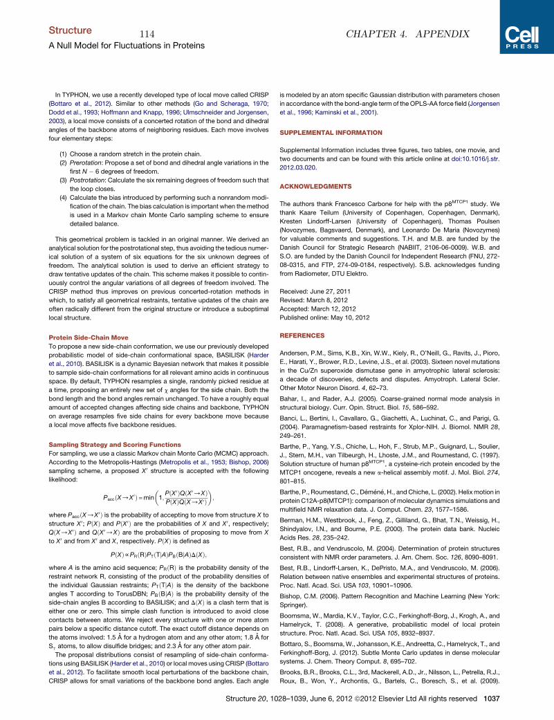
In TYPHON, we use a recently developed type of local move called CRISP

(Bottaro et al., 2012). Similar to other methods (Go and Scheraga, 1970;

Dodd et al., 1993; Hoffmann and Knapp, 1996; Ulmschneider and Jorgensen,

2003), a local move consists of a concerted rotation of the bond and dihedral

angles of the backbone atoms of neighboring residues. Each move involves

four elementary steps:

(1) Choose a random stretch in the protein chain.

(2) Prerotation: Propose a set of bond and dihedral angle variations in the

first N � 6 degrees of freedom.

(3) Postrotation: Calculate the six remaining degrees of freedom such that

the loop closes.

(4) Calculate the bias introduced by performing such a nonrandom modi-

fication of the chain. The bias calculation is important when themethod

is used in a Markov chain Monte Carlo sampling scheme to ensure

detailed balance.

This geometrical problem is tackled in an original manner. We derived an

analytical solution for the postrotational step, thus avoiding the tedious numer-

ical solution of a system of six equations for the six unknown degrees of

freedom. The analytical solution is used to derive an efficient strategy to

draw tentative updates of the chain. This scheme makes it possible to contin-

uously control the angular variations of all degrees of freedom involved. The

CRISP method thus improves on previous concerted-rotation methods in

which, to satisfy all geometrical restraints, tentative updates of the chain are

often radically different from the original structure or introduce a suboptimal

local structure.

Protein Side-Chain Move

To propose a new side-chain conformation, we use our previously developed

probabilistic model of side-chain conformational space, BASILISK (Harder

et al., 2010). BASILISK is a dynamic Bayesian network that makes it possible

to sample side-chain conformations for all relevant amino acids in continuous

space. By default, TYPHON resamples a single, randomly picked residue at

a time, proposing an entirely new set of c angles for the side chain. Both the

bond length and the bond angles remain unchanged. To have a roughly equal

amount of accepted changes affecting side chains and backbone, TYPHON

on average resamples five side chains for every backbone move because

a local move affects five backbone residues.

Sampling Strategy and Scoring Functions

For sampling, we use a classic Markov chain Monte Carlo (MCMC) approach.

According to the Metropolis-Hastings (Metropolis et al., 1953; Bishop, 2006)

sampling scheme, a proposed X0 structure is accepted with the following

likelihood:

PaccðX/X0Þ=min

�1;PðX 0ÞQðX0/XÞPðXÞQðX/X 0Þ

�;

where PaccðX/X0Þ is the probability of accepting to move from structure X to

structure X0; PðXÞ and PðX0Þ are the probabilities of X and X0, respectively;

QðX/X0Þ and QðX0/XÞ are the probabilities of proposing to move from X

to X0 and from X0 and X, respectively. PðXÞ is defined as

PðXÞfPRðRÞPTðTjAÞPBðBjAÞDðXÞ;

where A is the amino acid sequence; PRðRÞ is the probability density of the

restraint network R, consisting of the product of the probability densities of

the individual Gaussian restraints; PTðTjAÞ is the density of the backbone

angles T according to TorusDBN; PBðBjAÞ is the probability density of the

side-chain angles B according to BASILISK; and DðXÞ is a clash term that is

either one or zero. This simple clash function is introduced to avoid close

contacts between atoms. We reject every structure with one or more atom

pairs below a specific distance cutoff. The exact cutoff distance depends on

the atoms involved: 1.5 A for a hydrogen atom and any other atom; 1.8 A for

Sg atoms, to allow disulfide bridges; and 2.3 A for any other atom pair.

The proposal distributions consist of resampling of side-chain conforma-

tions using BASILISK (Harder et al., 2010) or local moves using CRISP (Bottaro

et al., 2012). To facilitate smooth local perturbations of the backbone chain,

CRISP allows for small variations of the backbone bond angles. Each angle

is modeled by an atom specific Gaussian distribution with parameters chosen

in accordance with the bond-angle term of theOPLS-AA force field (Jorgensen

et al., 1996; Kaminski et al., 2001).

SUPPLEMENTAL INFORMATION

Supplemental Information includes three figures, two tables, one movie, and

two documents and can be found with this article online at doi:10.1016/j.str.

2012.03.020.

ACKNOWLEDGMENTS

The authors thank Francesco Carbone for help with the p8MTCP1 study. We

thank Kaare Teilum (University of Copenhagen, Copenhagen, Denmark),

Kresten Lindorff-Larsen (University of Copenhagen), Thomas Poulsen

(Novozymes, Bagsvaerd, Denmark), and Leonardo De Maria (Novozymes)

for valuable comments and suggestions. T.H. and M.B. are funded by the

Danish Council for Strategic Research (NABIIT, 2106-06-0009). W.B. and

S.O. are funded by the Danish Council for Independent Research (FNU, 272-

08-0315, and FTP, 274-09-0184, respectively). S.B. acknowledges funding

from Radiometer, DTU Elektro.

Received: June 27, 2011

Revised: March 8, 2012

Accepted: March 12, 2012

Published online: May 10, 2012

REFERENCES

Andersen, P.M., Sims, K.B., Xin, W.W., Kiely, R., O’Neill, G., Ravits, J., Pioro,

E., Harati, Y., Brower, R.D., Levine, J.S., et al. (2003). Sixteen novel mutations

in the Cu/Zn superoxide dismutase gene in amyotrophic lateral sclerosis:

a decade of discoveries, defects and disputes. Amyotroph. Lateral Scler.

Other Motor Neuron Disord. 4, 62–73.

Bahar, I., and Rader, A.J. (2005). Coarse-grained normal mode analysis in

structural biology. Curr. Opin. Struct. Biol. 15, 586–592.

Banci, L., Bertini, I., Cavallaro, G., Giachetti, A., Luchinat, C., and Parigi, G.

(2004). Paramagnetism-based restraints for Xplor-NIH. J. Biomol. NMR 28,

249–261.

Barthe, P., Yang, Y.S., Chiche, L., Hoh, F., Strub, M.P., Guignard, L., Soulier,

J., Stern, M.H., van Tilbeurgh, H., Lhoste, J.M., and Roumestand, C. (1997).

Solution structure of human p8MTCP1, a cysteine-rich protein encoded by the

MTCP1 oncogene, reveals a new a-helical assembly motif. J. Mol. Biol. 274,

801–815.

Barthe, P., Roumestand, C., Demene, H., and Chiche, L. (2002). Helixmotion in

protein C12A-p8(MTCP1): comparison of molecular dynamics simulations and

multifield NMR relaxation data. J. Comput. Chem. 23, 1577–1586.

Berman, H.M., Westbrook, J., Feng, Z., Gilliland, G., Bhat, T.N., Weissig, H.,

Shindyalov, I.N., and Bourne, P.E. (2000). The protein data bank. Nucleic

Acids Res. 28, 235–242.

Best, R.B., and Vendruscolo, M. (2004). Determination of protein structures

consistent with NMR order parameters. J. Am. Chem. Soc. 126, 8090–8091.

Best, R.B., Lindorff-Larsen, K., DePristo, M.A., and Vendruscolo, M. (2006).

Relation between native ensembles and experimental structures of proteins.

Proc. Natl. Acad. Sci. USA 103, 10901–10906.

Bishop, C.M. (2006). Pattern Recognition and Machine Learning (New York:

Springer).

Boomsma, W., Mardia, K.V., Taylor, C.C., Ferkinghoff-Borg, J., Krogh, A., and

Hamelryck, T. (2008). A generative, probabilistic model of local protein

structure. Proc. Natl. Acad. Sci. USA 105, 8932–8937.

Bottaro, S., Boomsma,W., Johansson, K.E., Andreetta, C., Hamelryck, T., and

Ferkinghoff-Borg, J. (2012). Subtle Monte Carlo updates in dense molecular

systems. J. Chem. Theory Comput. 8, 695–702.

Brooks, B.R., Brooks, C.L., 3rd, Mackerell, A.D., Jr., Nilsson, L., Petrella, R.J.,

Roux, B., Won, Y., Archontis, G., Bartels, C., Boresch, S., et al. (2009).

Structure




CHARMM: the biomolecular simulation program. J. Comput. Chem. 30, 1545–

1614.

Cornilescu, G., Marquardt, J.L., Ottiger, M., and Bax, A. (1998). Validation of

protein structure from anisotropic carbonyl chemical shifts in a dilute liquid

crystalline phase. J. Am. Chem. Soc. 120, 6836–6837.

de Groot, B.L., van Aalten, D.M., Scheek, R.M., Amadei, A., Vriend, G., and

Berendsen, H.J. (1997). Prediction of protein conformational freedom from

distance constraints. Proteins 29, 240–251.

Ding, F., and Dokholyan, N.V. (2008). Dynamical roles of metal ions and the di-

sulfide bond in Cu, Zn superoxide dismutase folding and aggregation. Proc.

Natl. Acad. Sci. USA 105, 19696–19701.

Dobson, C.M. (2003). Protein folding and misfolding. Nature 426, 884–890.

Dodd, L., Boone, T., and Theodorou, D.N. (1993). A concerted rotation algo-

rithm for atomistic Monte Carlo simulation of polymer melts and glasses.

Mol. Phys. 78, 961–996.

Doucet, N., Watt, E.D., and Loria, J.P. (2009). The flexibility of a distant loop

modulates active site motion and product release in ribonuclease A.

Biochemistry 48, 7160–7168.

Doucet, N., Jayasundera, T.B., Simonovi�c, M., and Loria, J.P. (2010). The

crystal structure of ribonuclease A in complex with thymidine-30-monophos-

phate provides further insight into ligand binding. Proteins 78, 2459–2468.

Fernandez, A. (2010). Transformative Concepts for Drug Design: Target

Wrapping (Heidelberg: Springer).

Fernandez, A., and Berry, R.S. (2002). Extent of hydrogen-bond protection

in folded proteins: a constraint on packing architectures. Biophys. J. 83,

2475–2481.

Fernandez, A., and Scott, R. (2003). Dehydron: a structurally encoded signal

for protein interaction. Biophys. J. 85, 1914–1928.

Fernandez, A., Sosnick, T.R., and Colubri, A. (2002). Dynamics of hydrogen

bond desolvation in protein folding. J. Mol. Biol. 321, 659–675.

Formoso, E., Matxain, J.M., Lopez, X., and York, D.M. (2010). Molecular

dynamics simulation of bovine pancreatic ribonuclease A-CpA and transition

state-like complexes. J. Phys. Chem. B 114, 7371–7382.

Go, N., and Scheraga, H.A. (1970). Ring closure and local conformational

deformations of chain molecules. Macromolecules 3, 178–187.

Hamelryck, T., Kent, J.T., and Krogh, A. (2006). Sampling realistic protein

conformations using local structural bias. PLoS Comput. Biol. 2, e131.

Hamelryck, T., Borg, M., Paluszewski, M., Paulsen, J., Frellsen, J., Andreetta,

C., Boomsma, W., Bottaro, S., and Ferkinghoff-Borg, J. (2010). Potentials of

mean force for protein structure prediction vindicated, formalized and gener-

alized. PLoS ONE 5, e13714.

Harder, T., Boomsma, W., Paluszewski, M., Frellsen, J., Johansson, K.E., and

Hamelryck, T. (2010). Beyond rotamers: a generative, probabilistic model of

side chains in proteins. BMC Bioinformatics 11, 306.

Henzler, A.M., and Rarey, M. (2010). In pursuit of fully flexible protein-ligand

docking: modeling the bilateral mechanism of binding. Mol. Inform. 29,

164–173.

Hess, B., Kutzner, C., Van Der Spoel, D., and Lindahl, E. (2008). Gromacs 4:

algorithms for highly efficient, load-balanced, and scalable molecular simula-

tion. J. Chem. Theory Comput. 4, 435–447.

Hinsen, K. (1998). Analysis of domain motions by approximate normal mode

calculations. Proteins 33, 417–429.

Hoffmann, D., and Knapp, E.W. (1996). Protein dynamics with off-latticeMonte

Carlo moves. Phys. Rev. E Stat. Phys. Plasmas Fluids Relat. Interdiscip.

Topics 53, 4221–4224.

Jacobs, D.J., Rader, A.J., Kuhn, L.A., and Thorpe, M.F. (2001). Protein flexi-

bility predictions using graph theory. Proteins 44, 150–165.

Jorgensen,W.L., Maxwell, D.S., and Tirado-Rives, J. (1996). Development and

testing of the OPLS all-atom force field on conformational energetics and

properties of organic liquids. J. Am. Chem. Soc. 118, 11225–11236.

Kabsch, W., and Sander, C. (1983). Dictionary of protein secondary structure:

pattern recognition of hydrogen-bonded and geometrical features.

Biopolymers 22, 2577–2637.

Kaminski, G.A., Friesner, R.A., Tirado-Rives, J., and Jorgensen, W.L. (2001).

Evaluation and reparametrization of the OPLS-AA force field for proteins via

comparison with accurate quantum chemical calculations on peptides.

J. Phys. Chem. B 105, 6474–6487.

Karplus, M., and McCammon, J.A. (2002). Molecular dynamics simulations of

biomolecules. Nat. Struct. Biol. 9, 646–652.

Kimber, M.S., Yu, A.Y.H., Borg, M., Leung, E., Chan, H.S., and Houry, W.A.

(2010). Structural and theoretical studies indicate that the cylindrical protease

ClpP samples extended and compact conformations. Structure 18, 798–808.

Klepeis, J.L., Lindorff-Larsen, K., Dror, R.O., and Shaw, D.E. (2009). Long-

timescale molecular dynamics simulations of protein structure and function.

Curr. Opin. Struct. Biol. 19, 120–127.

Kuzmanic, A., and Zagrovic, B. (2010). Determination of ensemble-average

pairwise root mean-square deviation from experimental B-factors. Biophys.

J. 98, 861–871.

Lange, O.F., Lakomek, N.A., Fares, C., Schroder, G.F., Walter, K.F., Becker,

S., Meiler, J., Grubmuller, H., Griesinger, C., and de Groot, B.L. (2008).

Recognition dynamics up to microseconds revealed from an RDC-derived

ubiquitin ensemble in solution. Science 320, 1471–1475.

Laskowski, R.A., MacArthur, M.W., Moss, D.S., and Thorton, J.M. (1993).

PROCHECK: a program to check the stereochemical quality of protein

structures. J. Appl. Cryst. 26, 283–291.

Leonidas, D.D., Maiti, T.K., Samanta, A., Dasgupta, S., Pathak, T., Zographos,

S.E., and Oikonomakos, N.G. (2006). The binding of 30-N-piperidine-4-

carboxyl-30-deoxy-ara-uridine to ribonuclease A in the crystal. Bioorg. Med.

Chem. 14, 6055–6064.

Levitt, M., Sander, C., and Stern, P.S. (1983). The normal modes of a protein:

native bovine pancreatic trypsin inhibitor. Int. J. Quantum Chem. 24 (Suppl 10 ),

181–199.

Lindorff-Larsen, K., Best, R.B., Depristo, M.A., Dobson, C.M., and

Vendruscolo, M. (2005). Simultaneous determination of protein structure and

dynamics. Nature 433, 128–132.

Lipari, G., and Szabo, A. (1982). Model-free approach to the interpretation of

nuclear magnetic resonance relaxation in macromolecules. 2. Analysis of

experimental results. J. Am. Chem. Soc. 104, 4559–4570.

Lipsitz, R.S., and Tjandra, N. (2004). Residual dipolar couplings in NMR

structure analysis. Annu. Rev. Biophys. Biomol. Struct. 33, 387–413.

Long, D., and Bruschweiler, R. (2011). In silico elucidation of the recognition

dynamics of ubiquitin. PLoS Comput. Biol. 7, e1002035.

Ma, J. (2005). Usefulness and limitations of normal mode analysis in modeling

dynamics of biomolecular complexes. Structure 13, 373–380.

Maragakis, P., Lindorff-Larsen, K., Eastwood, M.P., Dror, R.O., Klepeis, J.L.,

Arkin, I.T., Jensen, M.Ø., Xu, H., Trbovic, N., Friesner, R.A., et al. (2008).

Microsecond molecular dynamics simulation shows effect of slow loop

dynamics on backbone amide order parameters of proteins. J. Phys. Chem.

B 112, 6155–6158.

Mardia, K.V., and Jupp, P.E. (2000). Directional Statistics (New York: John

Wiley and Sons).

Marrink, S.J., Risselada, H.J., Yefimov, S., Tieleman, D.P., and de Vries, A.H.

(2007). The MARTINI force field: coarse grained model for biomolecular

simulations. J. Phys. Chem. B 111, 7812–7824.

McCammon, J.A., Gelin, B.R., and Karplus, M. (1977). Dynamics of folded

proteins. Nature 267, 585–590.

Metropolis, N., Rosenbluth, A.W., et al. (1953). Equations of state calculations

by fast computing machines. J. Chem. Phys. 21, 1087–1092.

Olsson, S., Boomsma, W., Frellsen, J., Bottaro, S., Harder, T., Ferkinghoff-

Borg, J., and Hamelryck, T. (2011). Generative probabilistic models extend

the scope of inferential structure determination. J. Magn. Reson. 213,

182–186.

Pasinelli, P., and Brown, R.H. (2006). Molecular biology of amyotrophic lateral

sclerosis: insights from genetics. Nat. Rev. Neurosci. 7, 710–723.

Ramachandran, G.N., Ramakrishnan, C., and Sasisekharan, V. (1963).

Stereochemistry of polypeptide chain configurations. J. Mol. Biol. 7, 95–99.

Structure




Ramage, R., Green, J., Muir, T.W., Ogunjobi, O.M., Love, S., and Shaw, K.

(1994). Synthetic, structural and biological studies of the ubiquitin system:

the total chemical synthesis of ubiquitin. Biochem. J. 299, 151–158.

Schrodinger, L. (2010). The PyMOL molecular graphics system (version 1

1.3r1), Schrodinger, LLC.

Seeliger, D., and De Groot, B.L. (2009). tCONCOORD-GUI: visually supported

conformational sampling of bioactive molecules. J. Comput. Chem. 30, 1160–

1166.

Seeliger, D., and de Groot, B.L. (2010). Conformational transitions upon ligand

binding: holo-structure prediction from apo conformations. PLoS Comput.

Biol. 6, e1000634.

Seeliger, D., Haas, J., and de Groot, B.L. (2007). Geometry-based sampling of

conformational transitions in proteins. Structure 15, 1482–1492.

Shaw, D.E., Maragakis, P., Lindorff-Larsen, K., Piana, S., Dror, R.O.,

Eastwood, M.P., Bank, J.A., Jumper, J.M., Salmon, J.K., Shan, Y., and

Wriggers, W. (2010). Atomic-level characterization of the structural dynamics

of proteins. Science 330, 341–346.

Showalter, S.A., and Bruschweiler, R. (2007). Quantitative molecular ensemble

interpretation of NMR dipolar couplings without restraints. J. Am. Chem. Soc.

129, 4158–4159.

Skjøt, M., De Maria, L., Chatterjee, R., Svendsen, A., Patkar, S.A., Ostergaard,

P.R., and Brask, J. (2009). Understanding the plasticity of the a/b hydrolase

fold: Lid swapping on the Candida antartica Lipase B results in chimeras

with interesting biocatalytical properties. Chembiochem 10, 520–527.

Strange, R.W., Yong, C.W., Smith, W., and Hasnain, S.S. (2007). Molecular

dynamics using atomic-resolution structure reveal structural fluctuations that

may lead to polymerization of human Cu-Zn superoxide dismutase. Proc.

Natl. Acad. Sci. USA 104, 10040–10044.

Suhre, K., and Sanejouand, Y.H. (2004). ElNemo: a normal mode web server

for protein movement analysis and the generation of templates for molecular

replacement. Nucleic Acids Res. 32 (Suppl 2 ), W610–W614.

Teilum, K., Olsen, J.G., and Kragelund, B.B. (2009a). Functional aspects of

protein flexibility. Cell. Mol. Life Sci. 66, 2231–2247.

Teilum, K., Smith, M.H., Schulz, E., Christensen, L.C., Solomentsev, G.,

Oliveberg, M., and Akke, M. (2009b). Transient structural distortion of metal-

free Cu/Zn superoxide dismutase triggers aberrant oligomerization. Proc.

Natl. Acad. Sci. USA 106, 18273–18278.

Tirion, M.M. (1996). Large amplitude elastic motions in proteins from a single-

parameter, atomic analysis. Phys. Rev. Lett. 77, 1905–1908.

Tjandra, N., Feller, S.E., Pastor, R.W., and Bax, A. (1995). Rotational diffusion

anisotropy of human ubiquitin from 15N NMR relaxation. J. Am. Chem. Soc.

117, 12562–12566.

Tjandra, N., Omichinski, J.G., Gronenborn, A.M., Clore, G.M., and Bax, A.

(1997). Use of dipolar 1H-15N and 1H-13C couplings in the structure determi-

nation of magnetically oriented macromolecules in solution. Nat. Struct. Biol.

4, 732–738.

Ulmschneider, J., and Jorgensen, W. (2003). Monte Carlo backbone sampling

for polypeptides with variable bond angles and dihedral angles using

concerted rotations and a Gaussian bias. J. Chem. Phys. 118, 4261–4272.

Ulrich, E.L., Akutsu, H., Doreleijers, J.F., Harano, Y., Ioannidis, Y.E., Lin, J.,

Livny, M., Mading, S., Maziuk, D., Miller, Z., et al. (2008). BioMagResBank.

Nucleic Acids Res. 36 (Database issue), D402–D408.

Uppenberg, J., Ohrner, N., Norin, M., Hult, K., Kleywegt, G.J., Patkar, S.,

Waagen, V., Anthonsen, T., and Jones, T.A. (1995). Crystallographic and

molecular-modeling studies of lipase B from Candida antarctica reveal

a stereospecificity pocket for secondary alcohols. Biochemistry 34, 16838–

16851.

van Gunsteren,W.F., Billeter, S.R., Eising, A.A., Hunenberger, P.H., Kruger, P.,

Mark, A.E., Scott, W.R.P., and Tironi, I.G. (1996). Biomolecular Simulation:

The GROMOS96 Manual and User Guide (Zurich, Switzerland: Verlag der

Fachvereine Hochschulverlag AG an der ETH Zurich).

Vriend, G. (1990). WHAT IF: a molecular modeling and drug design program.

J. Mol. Graph. 8, 52–56, 29.

Watt, E.D., Shimada, H., Kovrigin, E.L., and Loria, J.P. (2007). The mechanism

of rate-limiting motions in enzyme function. Proc. Natl. Acad. Sci. USA 104,

11981–11986.

Wells, S., Menor, S., Hespenheide, B., and Thorpe, M.F. (2005). Constrained

geometric simulation of diffusive motion in proteins. Phys. Biol. 2, S127–S136.

Wlodarski, T., and Zagrovic, B. (2009). Conformational selection and induced

fit mechanism underlie specificity in noncovalent interactions with ubiquitin.

Proc. Natl. Acad. Sci. USA 106, 19346–19351.

Wlodawer, A., Svensson, L.A., Sjolin, L., and Gilliland, G.L. (1988). Structure of

phosphate-free ribonuclease A refined at 1.26 A. Biochemistry 27, 2705–2717.

Yang, L., Song, G., and Jernigan, R.L. (2009). Protein elastic network models

and the ranges of cooperativity. Proc. Natl. Acad. Sci. USA 106, 12347–12352.

Zachariae, U., Schneider, R., Velisetty, P., Lange, A., Seeliger, D., Wacker,

S.J., Karimi-Nejad, Y., Vriend, G., Becker, S., Pongs, O., et al. (2008). The

molecular mechanism of toxin-induced conformational changes in a potas-

sium channel: relation to C-type inactivation. Structure 16, 747–754.

Zheng, W., Brooks, B.R., and Hummer, G. (2007). Protein conformational

transitions explored by mixed elastic network models. Proteins 69, 43–57.

Structure




4.3. APPENDIX C: PHAISTOS 117

4.3 Appendix C: Phaistos

This paper presents the framework which has been in development in ThomasHamelrycks group to conduct Markov chain Monte Carlo simulations of pro-teins. The special features of PHAISTOS include the native incorporation ofthe probabilistic models of local protein structure TorusDBN and Basilisk,along with efficient sampling through generalized ensembles (Muninn).This is a co-author article. The paper is accepted for publication in Journalof Computational Chemistry. I was involved in extensive testing of theframework and have committed some core functionality.

PHAISTOS: A Framework for Markov Chain MonteCarlo Simulation and Inference of Protein Structure

Wouter Boomsma∗αβ, Jes Frellsenα, Tim Harderγα, Sandro Bottaroδε,Kristoffer E. Johanssonα, Pengfei Tianζ, Kasper Stovgaardα,

Christian Andreettaηα, Simon Olssonα, Jan Valentinα, Lubomir D. Antonovα,Anders S. Christensenθ, Mikael Borgια, Jan H. Jensenθ, Kresten Lindorff-Larsenα,

Jesper Ferkinghoff-Borgε, and Thomas Hamelryckα

March 26, 2013

Abstract

We present a new software framework for Markov chain Monte Carlo samplingfor simulation, prediction, and inference of protein structure. The software packagecontains implementations of recent advances in Monte Carlo methodology, such as ef-ficient local updates and sampling from probabilistic models of local protein structure.These models form a probabilistic alternative to the widely used fragment and rotamerlibraries. Combined with an easily-extendible software architecture, this makes PHAIS-TOS well-suited for Bayesian inference of protein structure from sequence and/or exper-imental data. Currently, two force-fields are available within the framework: PROFASIand the OPLS-AA/L force-field with the GB/SA solvent model. A flexible command-line and configuration-file interface allows users quickly to set up simulations with thedesired configuration.

PHAISTOS is released under the GNU General Public License v3.0. Source codeand documentation are freely available from http://phaistos.sourceforge.net. The soft-ware is implemented in C++, and has been tested on Linux and OSX platforms.

Keywords: Markov chain Monte Carlo simulation, protein structure, probabilisticmodels, local moves, conformational sampling

∗to whom correspondence should be addressedαDepartment of Biology, University of Copenhagen, 2200 Copenhagen, DenmarkβDepartment of Astronomy & Theoretical Physics, University of Lund, SE-223 62 Lund, SwedenγCenter for Bioinformatics, University of Hamburg, 20146 Hamburg, GermanyδScuola Internazionale Superiore di Studi Avanzati, 34136 Trieste, ItalyεDepartment of Biomedical Engineering, DTU Elektro, DTU, 2800 Kgs. Lyngby, DenmarkζNiels Bohr Institute, University of Copenhagen, 2100 Copenhagen, DenmarkηUni Computing, Uni Research AS, NorwayθDepartment of Chemistry, University of Copenhagen, 2100 Copenhagen, DenmarkιBILS, Science for Life Laboratory, Box 1031, 171 21 Solna, Sweden

1


We present a new software package for simulation and infer-ence of protein structure. The PHAISTOS framework con-tains a range of novel sampling techniques and probabilisticmodels, constituting a versatile toolkit for efficient simulationsof protein structure. The package provides tools for a varietyof tasks, including reversible folding simulations and proba-bilistic inference of protein structure from experimental data.The source code is released under an open source license andfull documentation is available online.

2


INTRODUCTION

Two methods dominate the field of molecular simulation: molecular dynamics (MD) andMarkov chain Monte Carlo (MCMC). The main difference between the methods lies in theway the system is updated in each iteration. MD involves iterating between calculatingthe forces exerted on each particle in the system, and using Newton’s equations of motionto update their positions. In contrast, MCMC is a statistical approach, where the goal isto generate samples from a probability distribution associated with the system, typically aBoltzmann distribution. MD has generally been regarded as best-suited for exploring densemolecular systems such as the native ensemble of proteins, while MCMC methods can bemore efficient for longer time scale simulations involving large structural rearrangements1.Using optimized move sets it has, however, been demonstrated that even in the denselypacked native state, MCMC can serve as an efficient alternative to MD2–4. In addition,the statistical nature of MCMC methods make them particularly well-suited for Bayesianinference of protein structure from experimental data5.

The freedom in the choice of moves in Monte Carlo simulations means that there is poten-tial progress to be made in designing new, improved move types, thereby further increasingthe time scales and molecular sizes amenable to simulation. In this paper, we present asoftware framework designed with this goal in mind. The PHAISTOS framework containsimplementations of recently developed tools that increase the efficiency and scope of MCMC-based simulations. Through a modular design, the software can easily be extended with newmove types and force-fields, making it possible to experiment with novel Monte Carlo strate-gies. Finally, using flexible configuration file and command line options, users can quickly setup simulations with any combination of moves, energy terms and other simulation settings.

By making our methods available in an easily extendible, open source framework, wehope to further encourage the use of MCMC for protein simulations, and promote the devel-opment of new MCMC methodologies for the simulation, prediction and inference of proteinstructure.

METHODOLOGY

The framework is split into four main types of components: moves, energy terms, observablesand Monte Carlo methods. For each of these types, a number of algorithms are available.Moves and energies are normally used in sets: a weighted set of moves is referred to as amove collection, while an energy function is composed of a weighted sum of energy terms.Observables are similar to energy terms, but are typically only evaluated at certain intervalsto extract statistics during a simulation. In the following description, each algorithm isannotated with its corresponding command line option name in a monospace font.

Moves

One of the main distinguishing features of the PHAISTOS package is efficient sampling,obtained through an elaborate set of both established and novel Monte Carlo moves. Eachmove stochastically modifies a protein chain in a specific way. Weighted sets of these moves

3


can be selected from the command line, allowing the user to easily experiment and fine-tune the set of moves for a given simulation scenario. All moves in PHAISTOS can beapplied such that detailed balance is obeyed, which ensures, if the sampling is ergodic,that simulations sample from a well-defined target distribution (e.g. the canonical or multi-canonical ensemble).

The framework contains many of the established moves from the literature, including var-ious pivot moves (move-pivot-uniform, move-pivot-local), the crankshaft/backrub localmove (move-crankshaft)6,7, the CRA local move (move-cra)8, and the semi-local biasedGaussian step (BGS) (move-semilocal)9. Side-chain conformational sampling can be doneeither from Gaussian distributions given by rotamer libraries (move-sidechain-rotamer)10

or through Gaussians centered around the current side-chain conformation (move-sidechain-local).

Moves using Probabilistic Models

PHAISTOS has broad support for sampling using biased proposals. Usually, if an MCMCsimulation were to be conducted without the presence of a force-field, a uniform distributionin configurational space would be obtained. In the case of biased sampling, moves are insteadallowed to follow a specific distribution during the simulation. This bias can then, optionally,be divided out so that it does not influence the final statistical ensemble, but only servesto increase sampling efficiency by focusing on the most important regions of conformationalspace. If the bias is left in, it corresponds to an implicit extra term in the energy function.

Typically, the bias is chosen to reflect prior knowledge about the local structure of themolecule. A good example is the common use of fragment and rotamer libraries for structureprediction11,12. These methods are used strictly for sampling, and the introduced bias is noteasily quantifiable, which also makes it difficult to ensure detailed balance for the Markovchain. In contrast, PHAISTOS includes a number of moves based on probabilistic models,which support both sampling of conformations and the evaluation of the bias introducedwith those moves. This makes them uniquely suited for use in MCMC simulations.

Four different structural, probabilistic models are available: FB5HMM models the Cαtrace of a protein13, COMPAS models a reduced single-particle representation of aminoacid side-chains, while TORUSDBN and BASILISK, respectively, model backbone and side-chain structure in atomic detail14,15. All models can be applied both as proposal distribu-tions in the form of Monte Carlo moves (move-backbone-dbn, move-sidechain-basilisk,move-sidechain-compas) and as probabilistic components of an energy function (energy-backbone-dbn, energy-basilisk, energy-compas). Figure 1 illustrates how dihedral anglesare sampled from a TORUSDBN-like model of the protein backbone. The practical detailson how probabilistic models can be incorporated in an energy function are discussed in theEnergy section below.

Efficient local updates

An important challenge in Monte Carlo simulations is to ensure efficient sampling in densestates where proposed conformational changes will have a high probability of containingself-collisions. In particular, pivot moves will typically have very poor acceptance rates inthis scenario. The solution is typically to expand the move set to include local moves, which

4


only change the atom positions within a small segment of the chain.In addition to various established local move methods from the literature, PHAISTOS

includes a novel method, called CRISP4 (move-crisp), which is particularly well-suited forthis problem. Unlike other local move approaches7,8, CRISP is able to generate updates toa segment of the chain without disrupting its local geometry. Often, local move algorithmsare designed as a two step process, where some angular degrees of freedom are modifiedstochastically (pre-rotation), while other are modified deterministically to bring the chainback to a closed state (post-rotation). From the work of Go and Scheraga16, it is known thatin general, six degrees of freedom are required for the post-rotation step. CRISP distinguishesitself from previous methods by merging these two steps, modifying the stochastic pre-rotation step so that it takes the resulting post-rotation step into account. More precisely, foreach application of the move, a random segment of the protein is selected, and a multivariateGaussian distribution is constructed over the angular change in the n−6 pre-rotation degreesof freedom δχpre

P (δχpre) ∝ exp

(−1

2δχTpreλ(Cn−6 + STC6S)δχpre

). (1)

Here, C is an inverse diagonal covariance matrix specifying the desired fluctuations forthe individual angular degrees of freedom, S is a linear transformation mapping the pre-rotational degrees of freedom to the corresponding post-rotational values, and λ is a scalingparameter determining the size of the move. In effect, to first order, the method samples froma distribution of closed chain structures, ensuring high quality local structure in all samples.We have recently shown that this has a dramatic impact on simulation performance, inparticular for dense molecular systems4.

Low acceptance rates are also sometimes observed in side-chain moves. When using a fine-grained force-field such as OPLS-AA/L, we have experienced that the standard resamplingof side-chains can be overly intrusive. Particularly in the case of side-chains involved inseveral simultaneous hydrogen bonds, traditional moves tend to break all hydrogen bonds atonce, typically leading to the rejection of such updates. To avoid this problem, PHAISTOSincludes a novel move (sidechain-local) that, for a given side-chain, randomly selects anatom that potentially participates in hydrogen bonds, and constrains its position using atechnique similar to that of the semi-local BGS backbone move4,9.

Energies

Two established force-fields are currently implemented within the framework: the PROFASIforce-field17, and the OPLS-AA/L18 force-field in combination with the GB/SA implicitsolvent model19. These represent two extremes in the range of force-fields available in theliterature: an ultrafast force-field modeling effective interactions in the presence of a solvent,and a classic fine-grained molecular mechanics force-field combined with a more accurateimplicit solvent model. The two forcefields were selected to provide support for a broad rangeof simulation tasks. The efficiency of the PROFASI forcefield makes it possible readily toconduct reversible folding simulations of peptides and small proteins17. The OPLS forcefieldin combination with the GB/SA solvent model is more accurate, but also significantly slower,and is typically used for exploring the details of native ensembles. It can also be used for

5


structure refinement, for instance of structures obtained in a reversible folding simulationusing PROFASI. For increased efficiency, all non-bonded force-field terms in both forcefieldshave been implemented using the chaintree data structure20, which avoids recalculation ofenergy contributions that are not modified in a given iteration of the simulation. Togetherwith effective local moves, this can result in a considerable computational speed-up.

PROFASI

The PROFASI force-field consists of four terms17

E = Eev + Ehb + Esc + Eloc (2)

where Eev captures excluded volume effects, Ehb is a hydrogen bond term, Esc is a side-chaininteraction term and Eloc concerns the local interactions along the chain. The excludedvolume potential is a simple r−12 interaction between all atom pairs, where r denotes thedistance between the atoms. The strength of a hydrogen bond in PROFASI depends onthe detailed geometry of the bond, parameterized through the N-H-O and H-O-C angles.The side-chain potential consists of a charge-charge and a hydrophobicity contribution. Foreach residue pair, these consist of a product between a conformation-dependent contactstrength and an energy that depends on the specific amino acid types involved in the bond.Finally, the local energy term captures interactions between partial charges in neighbouringpeptide units along the chain, with a correction term for improved consistency with theRamachandran plot, and a side-chain torsion potential. Since bond angles and bond lengthsare assumed fixed during PROFASI simulations, no further local interactions are included.

A distinguishing feature of the PROFASI force-field is the presence of a global interactioncutoff of 4.5A. While this necessarily excludes various long range interactions, it is also oneof the main reasons behind the efficiency of the force-field. Despite this restriction, the force-field has been demonstrated to successfully fold a range of peptides and small proteins17,while still being fast enough for many-body aggregation simulations21,22.

OPLS-AA/L

In contrast to PROFASI, the OPLS-AA/L force-field includes local terms for bond angles,bond lengths and torsions. The bond angle and bond length potentials are simple harmonicterms, while the torsion term has the form18

Etorsion =∑

i

3∑

j=1

wj(1 + (−1)j+1 cos(jθi)) (3)

where the outer sum iterates over all dihedrals θi. The non-bonded interactions includestandard Lennard-Jones and Coulomb potentials

Enb =∑

i>j

wij

(4εij

((σijrij

)12

−(σijrij

)6)

+1

4πε0

qiqjrij

)(4)

where rij is the distance between atoms i and j, qi and qj are the corresponding partialcharges, ε0 is the vacuum permittivity and σij and εij are calculated using the combination

6


rules σij =√σiσj and εij =

√εiεj. Finally, wij works to exclude interactions between atoms

that are separated by only a few covalent bonds. Thus, wij = 0.0 for direct neighbours (1,2)and pairs separated by a single other atom (1,3), wij = 0.5 for pairs separated by two atoms(1,4), and wij = 1.0 for all others.

Our implementation of OPLS-AA/L follows that of the TINKER simulation package23.We ensured that energies produced by our program match those obtained when runningTINKER.

GB/SA

The PROFASI force-field is parameterized to capture effective interactions in the presence ofa solvent. In contrast, OPLS should be combined with a suitable solvent model to reproducephysiological conditions. In order to model the effect of the solvent on hydrophobic inter-actions and electrostatics, we use the OPLS forcefield in combination with the GeneralizedBorn Surface Area (GB/SA) implicit solvent model19.

Many implicit solvent models express the solvation free energy Gsolv as a sum of non-polarand electrostatic contributions

Gsolv = Gnpol +Gpol (5)

Here, Gnpol is the free energy of solvating the molecule with all the partial charges set tozero, and Gpol is the reversible work required to increase the charges from zero to their fullvalues24. In GB/SA, the non-polar contribution Gnpol is assumed to be proportional to thesolvent accessible surface area, while the generalized Born approximation is used to calculatethe electrostatic solvation energy using the pairwise summation25

Gpol = − 1

8πε0

(1− 1

ε

) n∑

i,j

qiqjfGB

(6)

where ε is the dielectric constant of the solvent and qi is the partial charge of atom i.

fGB =√r2ij + αiαj exp (−r2

ij/4αiαj) is a function of the distance rij and of the so-called Born

radii α, which reflects the average distance of the charged atom to the dielectric medium. Forour implementation, the Born radii are calculated using an analytical expression proposedby Still and coworkers19.

Incorporating Probabilistic Models in the Energy Function

When using moves that are based on probabilistic models such as TORUSDBN or BASILISK,it gives rise to a bias in the simulation, which can be regarded as an implicit energy term.In PHAISTOS, the energy contributions of these probabilistic models can also be evaluatedexplicitly, by adding them as a term to the energy function. This makes it possible to use theprobabilistic models as energies in a simulation with a standard set of unbiased moves, or tocompensate for the bias of a move by adding the corresponding energy term with negativeweight. When used as energies, the values are reported in minus log-probabilities. In orderto facilitate the combination of classic energy terms with probabilistic terms, the energiesof physical force-fields such as PROFASI and OPLS-AA/L are likewise reported as minus

7


log-probabilities: they are multiplied by −1/kT , where T is the simulation temperature andk is the Boltzmann constant.

As an example, for the TORUSDBN-like model in Figure 1, the log-likelihood for a givenstate is

LL(X, A) = ln∑

H

P (X, A, H) (7)

= ln∑

H

P (X1|H1)P (A1|H1)P (H1)N∏

i=2

P (Xi|Hi)P (Ai|Hi)P (Hi|Hi−1)

where X, A and H are the sequences of angle pairs, amino acid labels, and hidden nodelabels, respectively, i is the residue index, and N is the sequence length. Each hidden nodelabel is the index of a component of the emission distributions of the model. For instance, theRamachandran distribution is modeled as a weighted sum of bivariate von Mises distributioncomponents14. The hidden nodes are “nuisance” parameters, and are therefore summed outin the evaluation of the likelihood. Note that the sum runs over all possible hidden nodesequences, a calculation which can be done efficiently using dynamic programming14.

Observables

Observables in PHAISTOS allow a user to extract information about the current state of asimulation. Examples of observables include root-mean-square-deviation (RMSD) (observable-rmsd) and radius of gyration (observable-rg). In addition, all energy terms are also avail-able as observables. A user can specify a selection of observables from the command line orsettings file, choosing how frequently they should be registered and in which format. Whilemost observables will return a single value, others have more elaborate outputs, such asdumping of complete structural states to PDB files (observable-pdb) or to a moleculartrajectory file in the Gromacs XTC format (observable-xtc-trajectory)26. Finally, ob-servables can be dumped to the header or as b-factors in outputted PDB-files. The lattermakes it possible to annotate structures with residue-specific information, such as the num-ber of contacts, degree of burial, or more sophisticated evaluations of the environment ofeach residue27.

Monte Carlo

Although PHAISTOS can be used for Monte Carlo minimization, the primary focus of theframework is Markov chain Monte Carlo simulation, where the goal is to produce samplesfrom the Boltzmann distribution corresponding to a given force-field at a specified temper-ature. All moves in PHAISTOS are therefore designed to be compatible with the propertyof detailed balance, in the sense that their proposal probabilities can be evaluated. That is,for a move from state x to state x′

π(x)P (x→ x′) = π(x′)P (x′ → x) (8)

8


where π(x) is the stationary distribution, and P (x → x′) is the probability of moving fromstate x to x′ using a given move. Factoring P (x→ x′) into a selection probability Ps and anacceptance probability Pα, we have

Pα(x→ x′)

Pα(x′ → x)=π(x′)Ps(x

′ → x)

π(x)Ps(x→ x′)(9)

Most of the moves are symmetric, in the sense that Ps(x′ → x)/Ps(x → x′) = 1. However,

for moves such as the local and semi-local moves, this is not the case, and it is important thatthis bias be correctly compensated for. Implementation-wise, each Move object is responsiblefor calculating the bias that it introduces, and the Monte Carlo class will then compensatefor it when necessary.

Metropolis-Hastings

The most common way to ensure that eq. (9) is fulfilled is to use the Metropolis-Hastings(MH) acceptance criterion

Pα(x→ x′) = min

(1,π(x′)Ps(x

′ → x)

π(x)Ps(x→ x′)

)(10)

This is the default simulation method used in PHAISTOS (monte-carlo-metropolis-hastings).It is useful for exploring near-native ensembles, and can be efficient when simulating at thecritical temperature of a system. However, for more complicated systems, MH simulationstend to spend excessive periods of time exploring local minima, leading to poor mixing andtherefore slow convergence.

Generalized Ensembles

To avoid the mixing problems associated with standard Metropolis-Hastings simulations,PHAISTOS includes support for conducting simulations in generalized ensembles28. Ratherthan sampling directly from the Boltzmann distribution, the central idea is to generatesamples from a modified distribution, and subsequently reweight the obtained statistics tothe Boltzmann distribution at a desired temperature. The acceptance criterion becomes

Pα(x→ x′) = min

(1,w(x′)Ps(x

′ → x)

w(x)Ps(x→ x′)

)(11)

for a given weight function w(x). The typical choice is the multi-canonical ensemble29,corresponding to a flat distribution over energies. That is, w(x) = 1/g(E(x)), where E(x) isthe energy associated with conformational state x, and g is the number of states associatedwith a given energy (density of states). Another example is the 1/k ensemble, which attemptsto provide ergodic sampling while maintaining primary focus on the low energy states30. In

this case, the weight function is w(x) = 1/k(E(x)), where k(E(x)) =∫ E(x)

−∞ g(E)dE. It can

be shown that this is approximately equivalent to a flat histogram over ln(E(x))30.We have recently developed an automated method, MUNINN, for estimating the weights

w in generalized ensemble simulations (http://muninn.sourceforge.net/). It employsthe generalized multi-histogram equations31, and uses a non-uniform adaptive binning of

9


the energy space, ensuring efficient scaling to large systems. In addition, MUNINN allowsweights to be restricted to cover a limited temperature range of interest. The MUNINNfunctionality is seamlessly integrated into PHAISTOS, and can be activated by selecting thecorresponding Monte Carlo engine (monte-carlo-muninn).

Monte Carlo Minimization

PHAISTOS contains a few simulation algorithms that are directed at optimization, ratherthan sampling. These include a simulated annealing class (monte-carlo-simulated-annealing)and a greedy Monte Carlo optimization class (monte-carlo-greedy-optimization), whichare useful in cases where the user is interested in a single low-energy structure, rather thana full structural ensemble.

Program Design

The framework is designed to be modular, both in software design and in the choices exposedto the user from the command line or settings file. As illustrated in the UML diagram inFigure 2, all energy terms are derived from the same base class, and implement the sameinterface. Energy functions can easily be constructed from the command line or settings fileby including the energy terms of interest. Moves and Monte Carlo simulation algorithms arestructured in a similar way. This design makes it straightforward to implement new energyterms, moves or simulation algorithms with little knowledge of the overall code. Iteratorsare provided for easy iteration over atoms or residues in a molecule. In addition, cachingand rapid determination of interacting atom pairs is made possible by an implementation ofthe chaintree algorithm20.

Finally, through a modular build-system, developers can readily write their own modulesutilizing the library. Modules are separate code entities that are auto-detected by the buildsystem when present, and can be enabled and disabled at compile time, making it easy toshare code among collaborators.

Example

We include a step-by-step walk-through of the PHAISTOS simulation process. The goal isto conduct a reversible folding simulation of the 20-residue beta3s peptide32, demonstratingseveral of the features described above.

The user interface of PHAISTOS is designed to make it as easy as possible to set upsimulations. Almost all options have default values, and it is therefore usually sufficient tosupply only a few input options to the program. The program behavior can then graduallybe fine-tuned using additional options in the configuration file later on. For this particularexample, we use the following command from the command line

$ ./phaistos --aa-file beta3s.aa \

--energy profasi-cached backbone-dbn[weight:-1] \

--move backbone-dbn sidechain-uniform semilocal-dbn-eh \

--threads 8 --temperature 283 \

10


--monte-carlo muninn[min-beta:0.6,max-beta:1.1] \

--observable backbone-dbn rmsd[reference-pdb-file:beta3s.pdb] \

--observable xtc-trajectory

The aa-file argument specifies that we are reading an amino acid sequence from a file. Theenergy and move options select the relevant energy terms and moves, respectively. In thiscase, we use a cached version of the PROFASI force-field, and sample using TORUSDBNmoves, uniformly distributed side-chain moves and BGS moves using the TORUSDBN asa prior. We specify that the simulation should be conducted in 8 parallel threads andset the temperature to 283K. MUNINN is chosen to be the Monte Carlo engine, using a β(inverse temperature) range of [0.6; 1.1]. These β factors are unit-less, specified relative to theinverse temperature, and thus correspond to a temperature range of [(1.1 · 1/283K)−1; (0.6 ·1/283K)−1] = [257K; 472K]. Finally, we specify that we wish to record observables aboutthe backbone-dbn energy, the RMSD to the native state, and dump structures to an XTCtrajectory file. Apart from the RMSD observable, we do not provide the program with anyinformation about the structure of the protein, and the simulation will therefore start in arandom extended state.

To illustrate the framework’s support for various types of biased sampling, this exampleuses a variant where the TORUSDBN bias is included in the sampling, and explicitly sub-tracted in the energy (i.e. the weight:-1 option of backbone-dbn). This means that the biascancels out when extracting statistics at β = 1, thus producing unbiased estimates at 283K.The simulation will produce a flat histogram over the expected energy range correspondingto the specified temperature range ([< E >257K ;< E >472K ]).

We ran PHAISTOS with the settings above on an eight-core 3.4GHz Intel Xeon pro-cessor for one week. Figure 3 gives an overview of the results. The free energy plot inFigure 3(a) shows the distribution of energy versus RMSD extracted directly from the sam-ples dumped during the simulation. Since the samples were generated using a generalizedensemble technique, they must be reweighted to retrieve the statistics according to the Boltz-mann distribution at the specified temperature. This is done using a script included in theMUNINN module, resulting in the plot in Figure 3(b).

To find representative structures in the ensemble, we use the PLEIADES clustering mod-ule33, included in the framework. Again, it is important to remember that the raw data areproduced in a generalize ensemble setting and must be reweighted. We ran the RMSD-basedweighted k-means method implemented in the PLEIADES module to select the highlightedstructures in Figure 3.

From the analysis above, we conclude that at 283K, the protein is marginally stable inthe PROFASI force-field, with native-like populations at 2A and 4A RMSD, but also a signif-icant population of unstructured or helical conformations. These results are in approximateagreement with experiments, which suggest a folded population of between 13% and 31%32.This result is compatible with a previously published simulation of the same protein usingan unbiased simulation technique17.

11


RESULTS

To illustrate the versatility of PHAISTOS, we highlight several recently published applica-tions of the framework.

Structure prediction and inference

An example of the applicability of PHAISTOS in the context of protein structure predictionis found in a recent study on potentials of mean force34. The study demonstrates howprobabilistic models of local protein structure such as TORUSDBN and BASILISK canbe combined with probabilistic models of nonlocal features, such as hydrogen bonding orcompactness, using a simple probabilistic technique.

The framework has also been applied for inference of protein structure from Small-angleX-ray scattering (SAXS) and Nuclear Magnetic Resonance (NMR) experimental data. SAXSdata contains low resolution information on the overall shape of a protein, which can be usefulfor determining the relative domain positions and orientations in multi-domain proteins orcomplexes. This can for instance be used to infer structural models of multi-domain proteinsconnected by flexible linkers, given the atomic structures of the individual domains. Suchcalculations require efficient back-calculation of SAXS curves, which is made possible througha coarse grained Debye method35,36.

NMR experimental data can provide high resolution structural information which canimprove the accuracy of a simulation. PHAISTOS contains preliminary support for sam-pling conditional on chemical shift data, which is known to contain substantial informationon the local structure of a protein37,38. Furthermore, the framework was recently used for in-ferential structure determination using pair-wise distances obtained from NOE experiments,with TORUSDBN and BASILISK as prior distribution for the protein’s backbone and sidechains39.

Efficient clustering

Efficiently clustering a large number of protein structures is an important task in proteinstructure prediction and analysis. Typically, clustering programs require costly RMSD cal-culations for many pairs in the set of structures. PHAISTOS contains a clustering modulecalled PLEIADES that uses a k-means clustering approach40 to reduce the number of pair-wise RMSD distance calculations. Furthermore, PLEIADES includes support for replacingthe RMSD distance computations with distances between vectors of Gauss integrals41, whichprovides dramatic computational speedups33.

Native ensembles

The energy landscape around the native state tends to be rugged, making it challenging tosample such states efficiently1. For these tasks, the CRISP backbone move is particularly wellsuited, given its ability to propose subtle, non-disruptive updates to the protein backbone.Monte Carlo simulations using this move were recently shown to explore conformational

12


space with an efficiency on par with molecular dynamics, outperforming the current state-of-the-art in local Monte Carlo move methods4.

The TYPHON module42 rapidly explores near-native ensembles by using the CRISPmove in combination with a user-defined set of non-local restraints. Local structure isunder the control of probabilistic models of the backbone (TORUSDBN) and side chains(BASILISK), while non-local interactions such as hydrogen bonds and disulfide bridges areheuristically imposed as Gaussian restraints. TYPHON can be seen as a “null model” of con-formational fluctuations in proteins: it rapidly explores the conformational space accessibleto a protein given a set of specified restraints.

DISCUSSION

The relevance of a new software package should be assessed relative to already existingpackages in the literature. We acknowledge that in our case, there are a number of suchalternatives already available. We describe the most important ones here, focusing on thedifferences to the framework presented in this paper.

Of the available Monte Carlo software packages, the ROSETTA package11 is perhapsthe most widely used, and has an impressive track record for protein structure predictionand design43. The package focuses primarily on structure/sequence prediction (optimiza-tion) rather than simulation, and consequently, many of the moves in ROSETTA are notcompatible with the property of detailed balance.

PHAISTOS also has some overlap with the PROFASI simulation package44, in the sensethat both implement the BGS move9 and the PROFASI energy function17. The PROFASIsimulation program was designed as a tool for studying protein aggregation, and is thushighly optimized for many-chain simulation using their lightweight forcefield and under theassumption of fixed bond angles. PHAISTOS aims to provide a greater flexibility in thechoice of energies and a wider selection of moves, and is not limited to a fixed bond-anglerepresentation.

The closest alternatives to PHAISTOS are perhaps the CAMPARI software package1 andthe Monte Carlo package in CHARMM2, which both provide functionality for conductingMarkov chain Monte Carlo simulations using various force-fields and moves. Compared withPHAISTOS, the selection of force-fields and moves differ, and the focus is different. Forinstance, PHAISTOS has a strong focus on sampling using probabilistic models of localstructure, which is not supported by either of the two alternatives.

The current version of the PHAISTOS framework has several limitations. To a userfamiliar with molecular dynamics software, the primary limitation will presumably be thelack of explicit solvent models in the framework. The large conformational moves that pro-vide the sampling advantage of Monte Carlo simulations are difficult to combine with anexplicit solvent representation. In line with other Monte Carlo simulation packages, PHAIS-TOS is therefore currently limited to implicit solvent simulations. Another limitation is thatPHAISTOS can currently only simulate a single polypeptide at a time. This restriction willbe removed in the next release of the software, which will also include implementations ofseveral new force-fields.

As the list of applications demonstrates, even in its current form, the framework provides

13


the necessary tools for conducting relevant MCMC simulations of protein systems. Theframework incorporates generalized ensembles and novel Monte Carlo moves, including movesthat incorporate structural priors as proposal distributions. These features are unique to thisframework, and have been shown to increase sampling efficiency considerably.

The software is freely available under the GNU General Public License v3.0. All sourcecode is fully documented using the Doxygen system (http://www.doxygen.org) and a usermanual is available for detailed descriptions on how to set up simulations. Both sources ofinformation are accessible via the PHAISTOS web site, http://phaistos.sourceforge.net.

ACKNOWLEDGMENTS

This work was supported by the Danish Council for Independent Research [FNU272-08-0315to W.B., FTP274-06-0380 to K.S, FTP09-066546 to S.O., J.V., FTP274-08-0124 to K.E.J.],the Danish Council for Strategic Research [NABIIT2106-06-0009 to J.F., Ti.H., C.A., M.B.],the Novo Nordisk STAR Program [A.S.C.], a Hallas-Møller stipend from the Novo NordiskFoundation [K.L.L.] and Radiometer (DTU) [S.B.].

14


References

1. A. Vitalis and R.V. Pappu, Annu. Rep. Comput. Chem. 2009, 5, 49–76.

2. J. Hu, A. Ma and A.R. Dinner, J. Comput. Chem. 2006, 27, 203–216.

3. J.P. Ulmschneider, M.B. Ulmschneider and A. Di Nola, J. Phys. Chem. B. 2006, 110,16733–16742.

4. S. Bottaro, W. Boomsma, K. E. Johansson, C. Andreetta, T. Hamelryck andJ. Ferkinghoff-Borg, J. Chem. Theory Comput. 2012, 8, 695–702.

5. M. Habeck, M. Nilges and W. Rieping, Phys. Rev. Lett. 2005, 94, 18105.

6. M. R. Betancourt, J. Chem. Phys. 2005, 123, 174905–174907.

7. C. Smith and T. Kortemme, J. Mol. Biol. 2008, 380, 742–756.

8. J. P. Ulmschneider and W. L. Jorgensen, J. Chem. Phys. 2003, 118, 4261–4271.

9. G. Favrin, A. Irback and F. Sjunnesson, J. Chem. Phys. 2001, 114, 8154–8158.

10. R. L. Dunbrack and F. E. Cohen, Protein Sci. 1997, 6, 1661–1681.

11. A. Leaver-Fay, M. Tyka, S.M. Lewis, O.F. Lange, J. Thompson, R. Jacak, K. Kaufman,P.D. Renfrew, C.A. Smith, W. Sheffler et al., Methods Enzymol. 2011, 487, 545–574.

12. T. Przytycka, Proteins. 2004, 57(2), 338–344.

13. T. Hamelryck, J.T. Kent and A. Krogh, Plos. Comput. Biol. 2006, 2, e131.

14. W. Boomsma, K.V. Mardia, C.C. Taylor, J. Ferkinghoff-Borg, A. Krogh and T. Hamel-ryck, Proc. Natl. Acad. Sci. U. S. A. 2008, 105, 8932.

15. T. Harder, W. Boomsma, M. Paluszewski, J. Frellsen, K.E. Johansson and T. Hamelryck,BMC Bioinformatics. 2010, 11, 306.

16. N. Go and H.A. Scheraga, Macromolecules. 1970, 3(2), 178–187.

17. A. Irback, S. Mitternacht and S. Mohanty, PMC Biophysics. 2009, 2, 2.

18. G.A. Kaminski, R.A. Friesner, J. Tirado-Rives and W.L. Jorgensen, J. Phys. Chem. B.2001, 105, 6474–6487.

19. D. Qiu, Shenkin P.S., F.P. Hollinger and W.C. Still, J. Phys. Chem. A. 1997, 101,3005–3014.

20. I. Lotan, F. Schwarzer, D. Halperin and J.C. Latombe, J. Comput. Biol. 2004, 11,902–932.

21. A. Irback and S. Mitternacht, Proteins. 2007, 71(1), 207–214.

15


22. D.W. Li, S. Mohanty, A. Irback and S. Huo, PLoS Comput. Biol. 2008, 4(12), e1000238.

23. J.W. Ponder and F.M. Richards, J. Am. Chem. Soc. 1987, 8(7), 1016–1024.

24. B. Roux and T. Simonson, Biophys. Chem. 1999, 78(1), 1–20.

25. W.C. Still, A. Tempczyk, R.C. Hawley and T. Hendrickson, J. Am. Chem. Soc. 1990,112(16), 6127–6129.

26. B. Hess, C. Kutzner, D. van der Spoel and E. Lindahl, J. Chem. Theory Comput. 2008,4(3), 435–447.

27. K.E. Johansson and T. Hamelryck, Proteins (In press). 2013.

28. U.H.E. Hansmann and Y. Okamoto, J Comput. Chem. 1997, 18, 920–933.

29. B.A. Berg and T. Neuhaus, Phys. Rev. Lett. 1992, 68(1), 9.

30. B. Hesselbo and RB Stinchcombe, Phys. Rev. lett. 1995, 74(12), 2151–2155.

31. J. Ferkinghoff-Borg, J. Eur. Phys. J. B. 2002, 29, 481–484.

32. E. De Alba, J. Santoro, M. Rico and M. Jimenez, Protein Sci. 1999, 8, 854–865.

33. T. Harder, M. Borg, W. Boomsma, P. Røgen and T. Hamelryck, Bioinformatics. 2012,28, 510–515.

34. T. Hamelryck, M. Borg, M. Paluszewski, J. Paulsen, J. Frellsen, C. Andreetta,W. Boomsma, S. Bottaro and J. Ferkinghoff-Borg, PLoS ONE. 2010, 5, e13714.

35. K. Stovgaard, C. Andreetta, J. Ferkinghoff-Borg and T. Hamelryck, BMC Bioinformat-ics. 2010, 11, 429.

36. N.G. Sgourakis, O.F. Lange, F. DiMaio, I. Andre, N.C. Fitzkee, P. Rossi, G.T. Monte-lione, A. Bax and D. Baker, J. Am. Chem. Soc. 2011, 133(16), 6288–6298.

37. A. Cavalli, X. Salvatella, C.M. Dobson and M. Vendruscolo, Proc. Natl. Acad. Sci. U.S. A. 2007, 104, 9615.

38. Y. Shen, O. Lange, F. Delaglio, P. Rossi, J.M. Aramini, G. Liu, A. Eletsky, Y. Wu, K.K.Singarapu, A. Lemak et al., Proc. Natl. Acad. Sci. U. S. A. 2008, 105, 4685.

39. S. Olsson, W. Boomsma, J. Frellsen, S. Bottaro, T. Harder, J. Ferkinghoff-Borg andT. Hamelryck, J. Magn. Reson. 2011, 213, 182–186.

40. S. Lloyd, IEEE Trans. Inf. Theory. 1982, 28, 129–137.

41. P. Røgen and B. Fain, Proc. Natl. Acad. Sci. U. S. A. 2003, 100, 119.

42. T. Harder, M. Borg, S. Bottaro, W. Boomsma, S. Olsson, J. Ferkinghoff-Borg andT. Hamelryck, Structure. 2012, 20, 1028 – 1039.

16


43. R. Das and D. Baker, Annu. Rev. Biochem. 2008, 77, 363–382.

44. A. Irback and S. Mohanty, J. Comput. Chem. 2006, 27(13), 1548–1555.

45. Schrodinger, LLC. The PyMOL Molecular Graphics System, Version 0.99rc6.

17


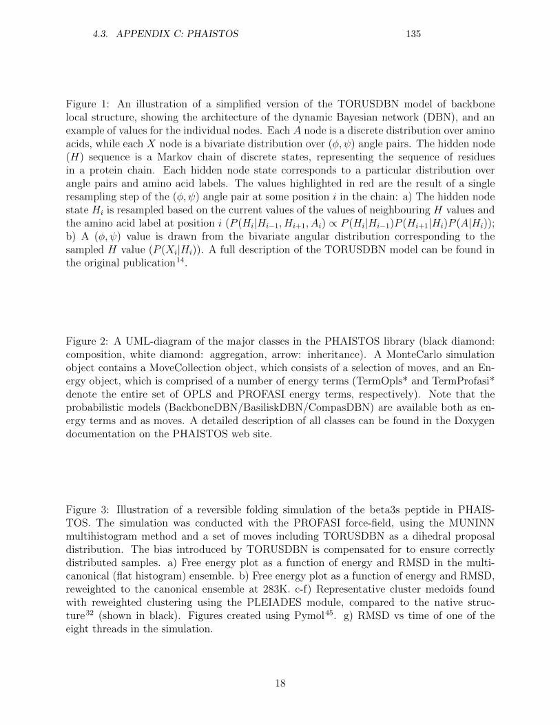
Figure 1: An illustration of a simplified version of the TORUSDBN model of backbonelocal structure, showing the architecture of the dynamic Bayesian network (DBN), and anexample of values for the individual nodes. Each A node is a discrete distribution over aminoacids, while each X node is a bivariate distribution over (φ, ψ) angle pairs. The hidden node(H) sequence is a Markov chain of discrete states, representing the sequence of residuesin a protein chain. Each hidden node state corresponds to a particular distribution overangle pairs and amino acid labels. The values highlighted in red are the result of a singleresampling step of the (φ, ψ) angle pair at some position i in the chain: a) The hidden nodestate Hi is resampled based on the current values of the values of neighbouring H values andthe amino acid label at position i (P (Hi|Hi−1, Hi+1, Ai) ∝ P (Hi|Hi−1)P (Hi+1|Hi)P (A|Hi));b) A (φ, ψ) value is drawn from the bivariate angular distribution corresponding to thesampled H value (P (Xi|Hi)). A full description of the TORUSDBN model can be found inthe original publication14.

Figure 2: A UML-diagram of the major classes in the PHAISTOS library (black diamond:composition, white diamond: aggregation, arrow: inheritance). A MonteCarlo simulationobject contains a MoveCollection object, which consists of a selection of moves, and an En-ergy object, which is comprised of a number of energy terms (TermOpls* and TermProfasi*denote the entire set of OPLS and PROFASI energy terms, respectively). Note that theprobabilistic models (BackboneDBN/BasiliskDBN/CompasDBN) are available both as en-ergy terms and as moves. A detailed description of all classes can be found in the Doxygendocumentation on the PHAISTOS web site.

Figure 3: Illustration of a reversible folding simulation of the beta3s peptide in PHAIS-TOS. The simulation was conducted with the PROFASI force-field, using the MUNINNmultihistogram method and a set of moves including TORUSDBN as a dihedral proposaldistribution. The bias introduced by TORUSDBN is compensated for to ensure correctlydistributed samples. a) Free energy plot as a function of energy and RMSD in the multi-canonical (flat histogram) ensemble. b) Free energy plot as a function of energy and RMSD,reweighted to the canonical ensemble at 283K. c-f) Representative cluster medoids foundwith reweighted clustering using the PLEIADES module, compared to the native struc-ture32 (shown in black). Figures created using Pymol45. g) RMSD vs time of one of theeight threads in the simulation.

18


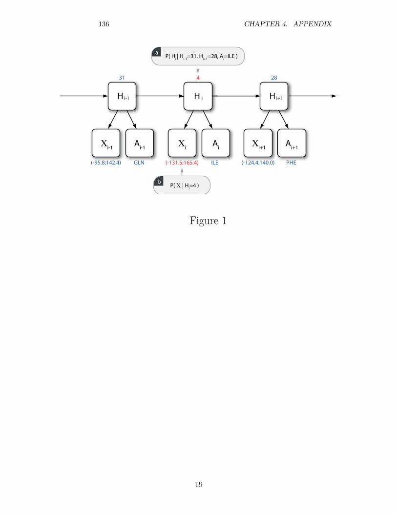
H i H i+1H i-1

Ai

Χi

Ai-1

Χi-1

Ai+1

Χi+1

GLN

31 4 28

(-95.8;142.4) (-131.5;165.4) (-124.4;140.0)ILE PHE

a

b

P( Hi | H

i-1=31, H

i+1=28, A

i=ILE )

P( Χi | H

i=4 )

Figure 1

19


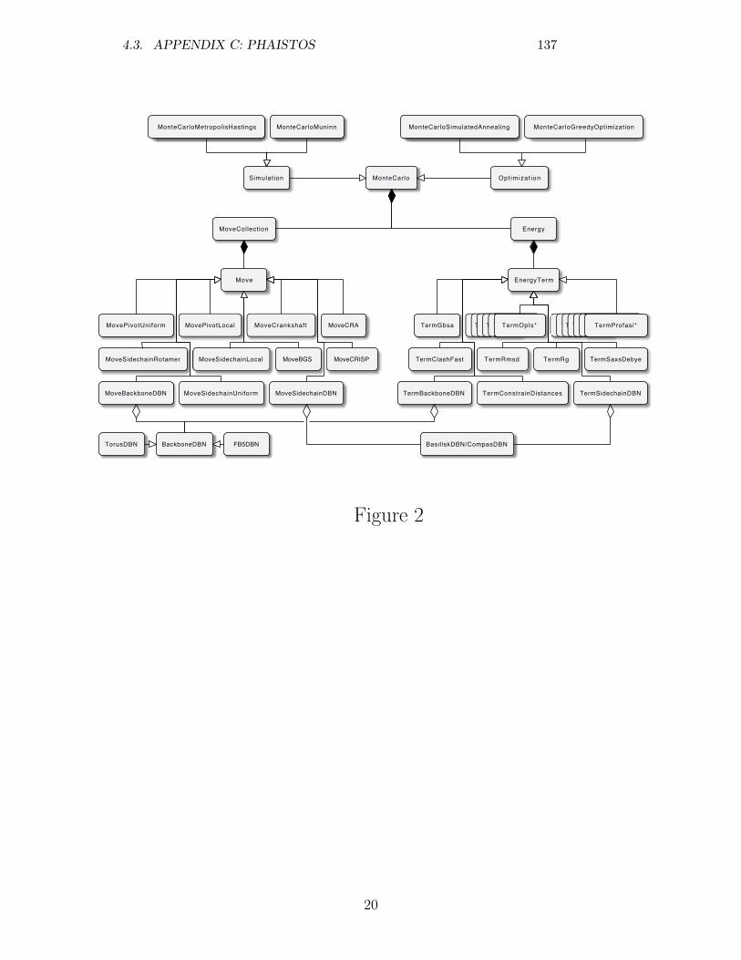
Energy

EnergyTerm

TermRmsd TermRg

TermBackboneDBN

TermClashFast

MonteCarlo

TermProfasiEV2TermProfasiHB2TermProfasiH2TermProfasiL2TermProfasiLS2TermProfasiSC2TTTTTTTTerermProfasiSC2TermProfasi*TermGbsa TermOplsAB2TermOplsBS2TermOplsC2TermOplsI2TermOplsT2TTTTTTTerermOplsT2TermOpls*

MoveCollection

MonteCarloMetropolisHastings MonteCarloSimulatedAnnealing

Simulation Opt imizat ion

Move

MoveCrankshaft

MoveBackboneDBN

MovePivotLocalMovePivotUniform

MoveSidechainLocal

MoveSidechainUniform

MoveCRA

MoveCRISPMoveBGS

MonteCarloMuninn

MoveSidechainRotamer TermSaxsDebye

TermConstrainDistancesMoveSidechainDBN

BackboneDBN FB5DBNTorusDBN BasiliskDBN/CompasDBN

TermSidechainDBN

MonteCarloGreedyOptimization

Figure 2

20


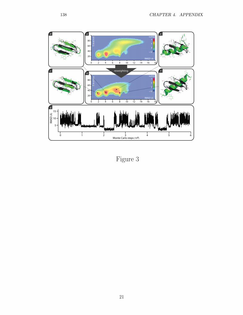
b

ad e

c

g

f

5

0 1 2 3 4 5 6

10

15

Monte Carlo steps (108)

RMSD

(Å)

●● ●

●

20

40

60

804

-ln(P(E))

6

8

>10

0 2 4 6 8 10 12 14 16 18

E (k

cal/

mo

l)

RMSD (Å)

20

40

60

80

0

4-ln(P(E))

6

8

>10

2 4 6 8 10 12 14 16 18

E (k

cal/

mo

l)

RMSD (Å)

reweighting

●●●

(kca

l/m

ol)

(kca

l/m

ol)

(kca

l/m

ol)

(kca

l/m

ol)

(kca

l/m

ol)

(kca

l/m

ol)

(kca

l/m

ol)

(kca

l/m

ol)

(kca

l/m

ol)

(kca

l/m

ol)

(kca

l/m

ol)

(kca

l/m

ol)

(kca

l/m

ol)

(kca

l/m

ol)

(kca

l/m

ol)

(kca

l/m

ol)

(kca

l/m

ol)

(kca

l/m

ol)

(kca

l/m

ol)

(kca

l/m

ol)

(kca

l/m

ol)

(kca

l/m

ol)

(kca

l/m

ol)

(kca

l/m

ol)

(kca

l/m

ol)

(kca

l/m

ol)

(kca

l/m

ol)

(kca

l/m

ol)

(kca

l/m

ol)

(kca

l/m

ol)

(kca

l/m

ol)

(kca

l/m

ol)

(kca

l/m

ol)

(kca

l/m

ol)

(kca

l/m

ol)

(kca

l/m

ol)

(kca

l/m

ol)

(kca

l/m

ol)

(kca

l/m

ol)

(kca

l/m

ol)

(kca

l/m

ol)

(kca

l/m

ol)

(kca

l/m

ol)

(kca

l/m

ol)

(kca

l/m

ol)

(kca

l/m

ol)

(kca

l/m

ol)

(kca

l/m

ol)

(kca

l/m

ol)

(kca

l/m

ol)

(kca

l/m

ol)

(kca

l/m

ol)

(kca

l/m

ol)

(kca

l/m

ol)

(kca

l/m

ol)

(kca

l/m

ol)

(kca

l/m

ol)

(kca

l/m

ol)

(kca

l/m

ol)

(kca

l/m

ol)

(kca

l/m

ol)

(kca

l/m

ol)

(kca

l/m

ol)

(kca

l/m

ol)

(kca

l/m

ol)

●●

888888888888888888888888●●●

Figure 3

21


Inference problems in structural biology: protein ... Olsson.pdf · Inference problems in...

Documents

Transcript of Inference problems in structural biology: protein ... Olsson.pdf · Inference problems in...