Inference on sets in finance

Victor Chernozhukov Emre Kocatulum Konrad Menzel

The Institute for Fiscal Studies Department of Economics, UCL

cemmap working paper CWP46/12

arX

iv:1

211.

4282

v1 [

stat

.AP]

19

Nov

201

2

INFERENCE ON SETS IN FINANCE

VICTOR CHERNOZHUKOV† EMRE KOCATULUM§ KONRAD MENZEL‡

Abstract. In this paper we consider the problem of inference on a class of sets de-

scribing a collection of admissible models as solutions to a single smooth inequality.

Classical and recent examples include, among others, the Hansen-Jagannathan (HJ)

sets of admissible stochastic discount factors, Markowitz-Fama (MF) sets of mean-

variances for asset portfolio returns, and the set of structural elasticities in Chetty

(2012)’s analysis of demand with optimization frictions. We show that the econometric

structure of the problem allows us to construct convenient and powerful confidence re-

gions based upon the weighted likelihood ratio and weighted Wald (directed weighted

Hausdorff) statistics. The statistics we formulate differ (in part) from existing statis-

tics in that they enforce either exact or first order equivariance to transformations of

parameters, making them especially appealing in the target applications. Moreover,

the resulting inference procedures are also more powerful than the structured projec-

tion methods, which rely upon building confidence sets for the frontier-determining

sufficient parameters (e.g. frontier-spanning portfolios), and then projecting them to

obtain confidence sets for HJ sets or MF sets. Lastly, the framework we put forward is

also useful for analyzing intersection bounds, namely sets defined as solutions to multi-

ple smooth inequalities, since multiple inequalities can be conservatively approximated

by a single smooth inequality. We present two empirical examples that show how the

new econometric methods are able to generate sharp economic conclusions.

Keywords: Hansen-Jagannathan bound, Markowitz-Fama bounds, Chetty bounds,

Mean-Variance sets, Optimization Frictions, Inference, Confidence Set

JEL classification: C10, C50

Date: March 2008 - this version: November 20, 2012. This paper was first presented at the March2008 CEMMAP conference on Inference in Partially Identified Models with Applications. We thankEnrique Sentana and Anna Mikusheva for pointing the relevance of structured projection approach asa benchmark for comparison, and Isaiah Andrews, Dan Greenwald, and Ye Luo for detailed commentson various drafts of the paper. We also thank Raj Chetty, Patrick Gagliardini, Raffaella Giacomini,Jerry Hausman, Olivier Scaillet, Nour Meddahi, Enno Mammen and participants of seminars at MIT,CEMMAP, 2009 Tolouse Conference on Financial Econometrics, and 2009 European Econometric So-ciety Meetings in Milan for useful discussion and comments.

1

2

1. Introduction

In this paper we consider the problem of inference on a class of sets describing a

collection of admissible models as solutions to a single smooth inequality:

Θ0 = θ ∈ Θ : m(θ) ≤ 0, (1.1)

where Θ ⊂ Rk is a compact parameter space, and m : Rk 7→ R is the inequality-

generating smooth function, which is estimable from the data. This structure arises in a

number of important examples in financial economics and public finance, as we explain

below via a sequence of examples. We show that this structure leads to highly-tractable

and powerful inference procedures, and demonstrate their usefulness in substantive em-

pirical examples. Furthermore, the structure could be used to conservatively approxi-

mate more complicated problems, where the sets of interest are given as intersections of

solutions to multiple smooth inequalities. (Indeed, in the latter case, we can conserva-

tively approximate the multiple inequalities by a single smooth inequality. The benefits

from doing so is the highly tractable, “regular” inference.)

Example 1: Mean-Variance Set for the Stochastic Discount Factor. In order to describe

the problem, we recall Cochrane (2005)’s assertion that the science of asset pricing could

be effectively summarized using the following two equations:

Pt = Et[Mt+1Xt+1],

Mt+1 = f(Zt+1, parameters),

where Pt is an asset price, Xt+1 is the asset payoff, Mt+1 is the stochastic discount

factor (SDF) or pricing kernel (PK), which is a function f of some data Zt+1 and pa-

rameters, and Et is the conditional expectation given information at time t. The set of

SDFs Mt that can price existing assets generally form a proper set, i.e. a set that is

not a singleton. SDFs are not unique as long as the existing payoffs to assets do not

span the entire universe of possible random payoffs. Dynamic asset pricing models pro-

vide families of potential SDFs, for example, the standard consumption model predicts

that an appropriate SDF can be stated in terms of the intertemporal marginal rate of

substitution:

Mt = βu′(Ct+1)

u′(Ct),

where u denotes a utility function parameterized by some parameters, Ct denotes con-

sumption at time t, and β denotes the subjective discount factor. Note that the investor’s

3

optimal consumption plan, and therefore the marginal rate of substitution, generally de-

pend on a set of additional state variables Zt, including lifetime wealth and non-capital

income. Hence, when markets are incomplete, asset prices alone do not in general pin

down a unique stochastic discount factor across different aggregate states of the economy

or across investors with different values of Zt.

An important empirical problem in the context of the CAPM is to check which fami-

lies of SDFs price the assets correctly and which do not. This reasoning forms the basis

for many approaches to estimation and tests for particular specifications of an asset

pricing model, most prominently Hansen and Singleton (1982)’s seminal analysis of the

consumption-based CAPM, see also Ludvigson (2012) for a survey of recent develop-

ments on the subject. One leading approach for performing the check is to see whether

the mean and standard deviation of SDFs (µ, σ) of the stochastic discount factor Mt are

admissible. Let K be a compact convex body in R2. The set of admissible means and

standard deviations in K

Θ0 := admissible pairs (µ, σ2) ∈ R2 ∩K,

is introduced by Hansen and Jagannathan (1991) and known as the Hansen-Jagannathan

(HJ) set. The boundary of that set ∂Θ0 is known as the HJ bound. In order to describe

the admissible pairs in a canonical setting, let v and Σ denote the vector of mean returns

and covariance matrix to assets 1, ..., N , which are assumed not to vary with information

sets at each period t. In the following, we consider the “minimal sufficient parameters”:

Svv = v′Σ−1v, Sv1 = v′Σ−11N , S11 = 1′NΣ−11N , (1.2)

where 1N is a column vector of ones. Then the minimum variance σ2HJ(µ) achievable by

a SDF given mean µ of the SDF is equal to

σ2HJ (µ) = (1− µv)′ Σ−1 (1− µv) = Svvµ

2 − 2Sv1µ+ S11.

Therefore, the HJ set is equal to

ΘHJ = (µ, σ)︸ ︷︷ ︸θ

∈ (R× R+) ∩K︸ ︷︷ ︸Θ

: σHJ (µ)− σ︸ ︷︷ ︸m(θ)

≤ 0.

That is,

Θ0 = θ ∈ Θ : mHJ (θ) ≤ 0.

4

Note that the inequality-generating function mHJ (θ) depends on the unknown means µ

and covariance of returns Σ via the minimal sufficient parameters, γ = (Svv, Sv1, S11)′,

so that we will write mHJ (θ) = mHJ(θ, γ).

Example 2: Mean-Variance Analysis of Asset Portfolios. Let us now describe the second

problem. The classical Markowitz (1952) problem is to minimize the variance of a

portfolio given some attainable level of return:

minw

Et[rp,t+1 − Et[rp,t+1]]2 such that Et[rp,t+1] = µ,

where rp,t+1 is the return of the portfolio, determined as rp,t+1 = w′rt+1, and w is a vector

of portfolio “weights” and rt+1 is a vector of returns on available assets. In a canonical

version of the problem, we have that the vector of mean returns v and covariance of

returns Σ do not vary with time period t, so that the problem becomes:

σM(µ) = minw

w′Σw such that w′v = µ.

An explicit solution for σM (µ) takes the form,

σ2M (µ) =

S11µ2 − 2Sv1µ+ Svv

SvvS11 − S2v1

,

where the minimal sufficient parameters γ = (Svv, Sv1, S11)′ are the same as in equation

(1.2).

Therefore given a compact convex body K ⊂ R2, the Markowitz (M) set of admissible

standard deviations and means in K is given by

ΘM = (µ, σ) ∈ (R× R+) ∩K : σM(µ)− σ ≤ 0 = θ ∈ Θ : mM (θ) ≤ 0,

where mM(θ) := σM (µ) − σ. The boundary of the set ΘM is known as the efficient

frontier. Note that as in HJ example, the inequality-generating function mM (θ) =

mM(θ, γ) depends on the unknown parameters, the means and covariance of returns, γ =

(Svv, Sv1, S11)′. We also note that in some applications, the complementary Markowitz

set is of interest:

ΘcM = θ ∈ Θ : −mM (θ) ≤ 0.

The inference on such sets thus also fall in our framework (1.1).

Mean-variance analysis for asset returns and the stochastic discount factor provides

powerful tools to summarize the opportunities for risk diversification in a given asset

market, and can serve as a basis for spanning and efficiency tests. The importance of

5

sampling error and the role of statistical inference in portfolio analysis has long been

recognized in the literature: Gibbons et al. (1989) develop regression-based efficiency

tests, and Britten-Jones (1999) considers inference on the tangency portfolio and tests for

portfolio efficiency; recent work by Penaranda and Sentana (2010) combines restrictions

derived from the two dual approaches to mean-variance analysis in order to derive more

powerful spanning tests for (sub-)markets; a summary of the recent literature on mean-

variance efficiency tests is provided by Sentana (2009). The econometric contribution of

this paper is quite distinct from and hence complementary to these previous efforts.

Example 3: Multi-Factor Efficient Frontiers. A third example due to Fama (1996)

extends the unconditional portfolio choice problem in Markowitz (1952) to multiple

sources of priced risk. More specifically, suppose that there exist k state variables

Zt = (z1t, . . . , zkt)′ (“factors”) such that (r′t, Z

′t)

′ are jointly normal (or, more gener-

ally, jointly spherical). We assume that Zt follows a K-variate standard normal (or

other spherical) distribution, and

Et[rt+1|Zt+1] = v +B′Zt+1

where v is an N -dimensional vector of average returns, and the k×N covariance matrix

B = [β1, . . . , βN ] = Covt(Zt+1, rt+1) gives the factor loadings for the vector of asset

returns. As in the previous examples, we denote the (unconditional) mean of asset

returns by v ∈ RN , and their covariance matrix with Σ. Note that for the purposes of

this example, we take rit to denote the excess return of asset i relative to a risk-free

asset with return rf .

This analysis is motivated by the investor’s lifetime consumption-investment problem,

where the state variables Zt denote other factors influencing prices for consumption

goods and the household’s income from wage labor or entrepreneurial activity in period

t. In particular the household not only faces a trade-off between mean and variance of

portfolio returns, but may also wish to use her portfolio to insure against price or income

shocks.

Specifically, we consider the problem constructing a minimum variance portfolio that

targets a mean return µ∗ and a vector β∗ of loadings respect to the factors Zt in the

absence of borrowing constraints. Denoting D := [v, B′] and δ∗ := (µ∗, β∗′)′, the efficient

portfolio weights w can be found by solving the program

minw

w′Σw s.t. D′w = δ∗. (1.3)

6

Note that since the investor has access to the risk-free asset and faces no short-sale

constraints, the portfolio weights w are not required to be nonnegative or sum up to

one. Solving this program yields efficient portfolio weights w∗ = Σ−1D(D′ΣD)−1δ∗ so

that the lower bound on the variance of a portfolio with beta equal to β and mean µ is

given by

σ2MF (µ, β) := (w∗)′Σw∗ = δ∗

′

(D′ΣD)−1δ∗.

The resulting multi-factor efficient frontier bounds the cone

ΘMF :=(µ∗, β∗′, σ)′ ∈ (Rk+1 × R+) ∩K : σMF (µ

∗, β∗)− σ ≤ 0

of feasible mean-variance-beta combinations, where K is some compact convex body

in Rk+2. Again, this cone can also be characterized by an inequality condition on the

moment function

mMF (θ, γ) :=√(µ∗, β∗′)(D′ΣD)−1(µ∗, β∗′)′ − σ

where θ = (µ∗, β∗′, σ)′ and γ = vec(D′ΣD).

Extending the two-fund theorem, Fama (1996) shows that we can always construct

k+2 different funds from the N assets that span the entire multi-factor efficient frontier.

In the presence of heterogeneity in preferences, wealth and consumption possibilities,

different investors will typically choose different points on the efficient cone, so that

only the entire set constitutes an adequate representation of the opportunities to insure

against different factor risks in the market.

Example 4: Bounds on Demand Elasticities. To illustrate the wider applicability of our

methods, we also consider inference on demand elasticities in the presence of an op-

timization friction. Chetty (2012) considers a household’s dynamic labor supply and

consumption problem and proposes bounds on price elasticities that allow for optimiza-

tion errors of unknown form but that are bounded in magnitude. His analysis assumes

that preferences can be represented by quasilinear flow utilities and lead to Marshallian

demand functions of the form

log x∗it(p) = α− ε log p + νit,

where p is the price of the good of interest, and νit a preference shock for household i in

period t. Here ε is the (constant) “structural” demand elasticity corresponding to the

first-best solution to the household’s planning problem.

7

Let U∗it be the discounted lifetime utility from following the optimal consumption

plan and let eit(x) denote the minimal expenditure needed to finance a utility level

U∗it under the constraint that xit is held fixed at x. The analysis then considers “small”

optimization errors in the households’ observed choice of xit such that for every period t,

the average utility loss measured in terms of the difference in expenditure as a percentage

of the optimal budget is bounded by some δ > 0, i.e.

1

N

∑Ni=1

eit(xit)− eit(x∗it(pt))

ptx∗it

≤ δ,

where the average is taken over a sample of households i = 1, . . . , N .

Chetty (2012) derives the lower and upper bounds εL and εU for the structural elas-

ticities that are compatible an observed elasticity εo given a price change ∆ log p, and

in the presence of an optimization error of δ > 0. This bound is given by the following

two inequalities

εo = εU − 2(2εUδ)

1/2

∆ log pand εo = εL + 2

(2εLδ)1/2

∆ log p

where δ is assumed to be small.1 With a few basic manipulations, we can obtain the

following equivalent characterization of the (δ, ε)-set as a lower bound for the distortion

needed to reconcile εo with a structural elasticity ε:

δ ≥ (ε− εo)2(∆ log p)2

8ε=: δOF (ε, ε

o,∆ log p) if and only if ε ∈ [εL, εU ]. (1.4)

Chetty (2012) gives several interpretations for this optimization friction, which could

result e.g. from adjustment costs or misperception of prices. In the context of the

consumption-CAPM model, Lettau and Ludvigson (2009) conducted a similar sensitiv-

ity analysis, allowing for optimization errors in terms of the Euler equations character-

izing the household’s optimal investment decision.

The resulting set of structural elasticity/optimization friction pairs (ε, δ) compatible

with the observed elasticity εo is given by

ΘOF :=(ε, δ) ∈ R

2+ : δOF (ε, ε

o,∆ log p)− δ ≤ 0.

1See equations (12) and (13) on pages 983-985 in Chetty (2012)

8

The bounds in equation (1.4) can therefore also be expressed as an inequality condition

on the moment function

mOF (θ, γ) :=(ε− εo)2(∆ log p)2

8ε− δ,

where θ = (ε, δ) and γ = εo, and ∆ log p will be regarded as a fixed design parameter.

In applications, one might be interested in intersections bounds from several studies in

order to obtain tighter bounds, as was done in Chetty (2012). As we discuss below and

illustrate in the empirical example, it is possible to perform this intersection in a smooth

fashion, retaining the general single-equation structure as given in (1.1).

1.1. Overview. The basic problem of this paper is to develop inference methods on

sets defined by nonlinear inequality restrictions, as the HJ and M sets, while accounting

for uncertainty in the estimation of parameters of the inequality-generating functions.

Specifically, the problem is to construct a confidence region R such that

limn→∞

PΘ0 ⊆ R = 1− α, dH(Θ0, R) = Op(1/√n),

where dH is the Hausdorff distance, defined below in (2.17). We will construct con-

fidence regions for the set Θ0 using LR and Wald-type Statistics, building on and si-

multaneously enriching the approaches suggested in Chernozhukov et al. (2007) and in

Beresteanu and Molinari (2008) and Molchanov (1998), respectively. We also would like

to ensure that confidence regions R are as small as possible and converge to Θ0 at the

fastest attainable speed.

Once R is constructed, we can test any composite hypotheses involving the parameter

θ without compromising the significance level. E.g. a typical application of the HJ

bounds determines which combinations of Θe the first two moments of the SDF generated

by a given family of economic models fall in the HJ set. Indeed, in that case Θe =

µ(), σ(), ∈ [0,∞), where is the elasticity of power utility function, and we can

check which values of γ give us overlap of Θe with the confidence set R for the HJ set.2

Similar comments about applicability of our approach go through for the M and MF sets

as well. We should also mention that our confidence regions R are also more powerful

than the structured projection methods, which rely upon building confidence sets for the

frontier-determining sufficient parameters (e.g. frontier-spanning portfolios), and then

projecting them to obtain confidence sets for HJ sets or MF sets. We demonstrate this

2In cases where curve 7→ µ(), 7→ σ() are estimated, we need to construct a confidence set Re forΘe and then look whether (and where) Re and R overlap to determine the plausible values of .

9

in the empirical section, where we compute the confidence sets for HJ sets based on our

approach and based on structured projection approach, and show that our confidence

interval is much smaller and lies strictly inside the confidence region based on structured

projections. We provide a theoretical explanation to this phenomenon in Section 2.5

Our procedure for inference using weighted Wald-type statistics complements other ap-

proaches based on the directed Hausdorff distance suggested in Beresteanu and Molinari

(2008) and Hausdorff distance in Molchanov (1998). By using weighting in the con-

struction of the Wald-type statistics, we make this approach asymptotically invariant

to parameter transformations, which results in noticeably sharper confidence sets, at

least in the canonical empirical example that we will show. These invariance properties

should be seen as complementary to questions of efficient estimation of the identified set

as studied by Kaido and Santos (2011); indeed, many types of confidence sets will all be

centered around the same efficient set estimate, and so we use invariance and precision

considerations to select amongst various potential constructions of sets.

Critchley et al. (1996) analyzed the geometric structure of Wald-type tests with non-

linear restrictions for point-identified problems and pointed out the beneficial role of

invariance of the distribution of the statistic with respect to reparameterizations. In

regular problems, the effect of nonlinearities on inference is typically asymptotically

negligible due to the delta method and its extensions. However, our results show that

for inference on sets with a nontrivial diameter, the effect of nonlinearities is of the

same order as that of sampling variation. In particular we propose inference procedures

that rely on quantities that are asymptotically pivotal and (asymptotically) invariant to

parameter transformation, and illustrate that procedures failing to meet these require-

ments lead to overly conservative inference. In particular, these conditions are not met

by the classical Hausdorff distance except in very special cases.

Thus, our construction is of independent interest for this type of inference and is

a useful complement to the work of Beresteanu and Molinari (2008) and Molchanov

(1998). Furthermore, our results on formal validity of the bootstrap for the weighed LR-

type andW-type statistics are also of independent interest (for the class of problems with

structures that are similar to those studied here; see Beresteanu and Molinari (2008) and

Kaido and Santos (2011) for related bootstrap results for Hausdorff statistics.)

The rest of the paper is organized as follows. In Section 2 we present our estimation

and inference results. In Section 3 we present an empirical example, illustrating the

constructions of confidence sets for HJ sets. In Section 4 we draw conclusions and

10

provide direction for further research. In the Appendix, we collect the proofs of the

main results.

2. Estimation and Inference Results

2.1. Basic Constructions. We first introduce our basic framework. We have a real-

valued inequality-generating function m(θ), and the set of interest is the solution of the

inequalities generated by the function m(θ) over a compact parameter space Θ ⊂ Rk:

Θ0 = θ ∈ Θ : m(θ) ≤ 0.

A natural estimator of Θ0 is its empirical analog

Θ0 = θ ∈ Θ : m(θ) ≤ 0,

where m(θ) is the estimate of the inequality-generating function. For example, in the

HJ and M examples, the estimate takes the form

m(θ) = m(θ, γ), γ = (Svv, Sv1, S11)′.

Remark 1 (Approximating Multiple Inequalities by A Single Smooth Inequality).

Throughout the paper, we will only consider the case of a single inequality restric-

tion, m : Θ → R satisfying certain smoothness conditions with respect to θ. However

this framework approximately encompasses the case of multiple inequalities, since it is

possible to conservatively approximate intersection bounds of the form g(θ) ≤ 0, where

g(θ) := (g1(θ), . . . , gJ(θ))′ represents a vector of constraints, by a single smooth bound

m(θ) ≤ 0. To be specific, we can form an inequality-generating function:

mλ(θ) := m(g1(θ), . . . , gJ(θ);λ) :=∑J

j=1

exp(λgj(θ))∑Jl=1 exp(λgl(θ))

gj(θ),

where λ ∈ R is a fixed, positive scalar. This function mλ is clearly smooth with respect

to the underlying function g, and is a conservative approximation to max1≤j≤J gj(θ) with

an explicit error bound, as shown by the following lemma.

Lemma 1 (Properties of Smooth Max). (i) We have that

m(g1, . . . , gJ , λ) ≤ 0 if max1≤j≤J

gj(θ) ≤ 0.

(ii) For any λ > 0, the approximation error obeys

sup(g1,...,gJ)′∈RJ

|max(g1, . . . , gJ)−m(g1, . . . , gJ , λ)| ≤ λ−1W

(J − 1

e

)

11

where e is Euler’s number, and the function W : R 7→ R is Lambert’s product logarithm

function, i.e. W (z) is defined as the solution w of the equation w expw = z. In

particular, W (z) ≥ 0 if z ≥ 0, and W (z) ≤ log(z) if z ≥ e.

This lemma implies that the approximation error relative to the max function (with

respect to the sup-norm) is inversely proportional to the smoothing parameter λ, where

the constant of proportionality grows only very slowly in J . In the paper we will state

our results and assumptions on estimation and inference directly in terms of the scalar

momentm(θ) = mλ(θ) and its empirical analog m(θ) := mλ(θ) := m(g1(θ), . . . , gJ(θ);λ).

We also consider the quantity 1/λ fixed at some small value.

Our proposals for confidence regions are based on (1) a LR-type statistic and (2) a

Wald-type statistic. The LR-based confidence region is

RLR :=θ ∈ Θ :

[√nm(θ)/s(θ)

]2+≤ k(1− α)

, (2.1)

where s(θ) is a weighting function; ideally, the standard error of m(θ); and k(1 − α) is

some suitable estimate of k(1− α), the (1− α)-quantile of the statistic

Ln = supθ∈Θ0

[√nm(θ)/s(θ)

]2+. (2.2)

Note that Ln is a LR-type statistic, as in Chernozhukov et al. (2007).

Next we shall consider confidence regions based on inverting a Wald-type statistic. In

order to eliminate boundary effects on the distribution of this statistic, we will need to

assume that the moment conditions, and therefore the set estimator, are well-defined in

a neighborhood of the parameter space. To this end, we define the distance of a point θ

to a set A ⊂ Rk as

d(θ, A) := infθ′∈A

‖θ − θ′‖.We let the set

Θδ := θ ∈ Rk : d(θ,Θ) ≤ δ

denote the δ-expansion of Θ in Rk for any δ > 0. We denote the natural set estimator

for Θ0 in the expansion of the parameter space by

Θ0,δ :=θ ∈ Θδ : m(θ) ≤ 0

.

We will see below that the behavior of the moment function near the boundary of the

parameter space is in general relevant for the statistical behavior of our procedure.

However, for the practical applications discussed in this paper, the restriction of the

12

parameter space Θ to a compact set is entirely for technical reasons, so that an extension

of the definitions to Θδ is unproblematic.

Given these definitions, our Wald-based confidence region is

RW := θ ∈ Θ : [√nd(θ, Θ0,δ)/w(θ)]

2 ≤ k(1− α), (2.3)

where w(θ) is a weighting function, particular forms of which we will suggest later; and

k(1− α) is a suitable estimate of k(1−α), the (1− α)-quantile of Wn, where Wn is the

weighted W-statistic

Wn := supθ∈Θ0

[√nd(θ, Θ0,δ)/w(θ)]

2. (2.4)

In the special case, where the weight function is flat, namely w(θ) = w for all θ, the W-

statistic Wn becomes the canonical directed Hausdorff distance (see Molchanov (1998),

and Beresteanu and Molinari (2008)):√

Wn ∝ d+(Θ0, Θ0,δ) = supθ∈Θ0

infθ′∈Θ0,δ

‖θ − θ′‖.

Remark 2 (Invariance Motivation for Weighed W-Statistics). The weighted W-statistic

(2.4) is generally not a distance, but we argue in Section 2.6 that it provides a very useful

extension/generalization of the canonical directed Hausdorff distance. Note that, like

any Euclidean norm, the Hausdorff distance is not invariant with respect to changes

in the scale of the different components of θ, which results in confidence regions that

are not equivariant to such transformations. Our empirical results below illustrate that

as a result, the shape of confidence sets alters dramatically as we change the weight

on different dimensions of the parameter space. In sharp contrast, the introduction of

certain types of weights makes the W-statistic (first-order) invariant to such transforma-

tions, as shown in Section 2.6, which makes the resulting confidence regions (first-order)

equivariant. As a result, in all of our empirical examples such weighting dramatically

improves the confidence regions (e.g. compare Figures 5 and 6 in the example concerning

inference on HJ sets.)

2.2. A Basic Limit Theorem for LR and W statistics. In this subsection, we de-

velop a basic result on the limit laws of the LR and W statistics. We will develop this

result under the following general regularity conditions:

Condition R. For some δ > 0, the inequality-generating functions m : Θδ → R and

its estimator m : Θδ → R are well-defined.

13

(R.1) The estimator m is n−1/2-consistent for m and asymptotically Gaussian, namely,

in the metric space of bounded functions ℓ∞(Θδ)

√n(m−m) G,

where G is a zero-mean Gaussian process with continuous paths a.s., and a non-

degenerate covariance function, i.e. infθ∈Θδ E[G2(θ)] > 0.

(R.2) Functions m and m admit continuous gradients ∇θm : Θδ 7→ Rk and ∇θm :

Θδ 7→ Rk with probability one, where

∇θm(θ) = ∇θm(θ) + op(1).

uniformly in θ ∈ Θδ. The gradient θ 7→ ∇θm is uniformly Lipschitz and

infθ∈Θδ ‖∇θm(θ)‖ > 0.

(R.3) Weighting functions s : Θδ 7→ R and s : Θδ 7→ R satisfy uniformly in θ ∈ Θδ

s(θ) = s(θ) + op(1), w(θ) = w(θ) + op(1),

where s : Θδ 7→ R+ and w : Θδ 7→ R+ are continuous functions with values

bounded away from zero.

In Condition R.1, we require the estimates of the inequality-generating functions to

satisfy a uniform central limit theorem. Many sufficient conditions for this are provided

by the theory of empirical processes, see e.g. van der Vaart and Wellner (1996). In our

finance examples, this condition will follow from asymptotic normality of the estimates of

the mean returns and covariance of returns. In Condition R.2, we require that gradient

of the estimate of the inequality-generating function be consistent for the gradient of

the inequality-generating function. Moreover, we require that the norm ‖∇θm(θ)‖ be

bounded away from zero, which is an identification condition and allows us to estimate,

at a parametric rate, the boundary of the set Θ0, which we define as

∂Θ0 := θ ∈ Θ : m(θ) = 0.

In Condition R.3, we require that the estimates of the weight functions be consistent,

and the weight functions be well-behaved.

Under these conditions we can state the following general result.

14

Theorem 1. (Limit Laws of LR and W Statistics). Under Condition R

Ln L, L = supθ∈∂Θ0

[G(θ)

s(θ)

]2

+

, (2.5)

Wn W, W = supθ∈∂Θ0

[G(θ)

‖∇θm(θ)‖ · w(θ)

]2

+

, (2.6)

where both W and L have distribution functions that are continuous at their (1 − α)-

quantiles for α < 1/2. Furthermore, if

w(θ) =s(θ)

‖∇θm(θ)‖ + op(1),

uniformly in θ ∈ Θδ, then the two statistics are asymptotically equivalent:

Wn = Ln + op(1).

In particular, this equivalence occurs if w(θ) = ‖∇θm(θ)‖/s(θ).

We see from this theorem that the LR and W statistics converge in law to well-behaved

random variables that are continuous transformations of the limit Gaussian process G.

Moreover, we see that under an appropriate choice of the weighting functions, the two

statistics are asymptotically equivalent.

For our application to HJ and MF sets, the following conditions will be sufficient.

Condition C.

(C.1) We have that m(θ) = m(θ, γ0), where γ0 ∈ Γ ⊂ Rd, for all θ ∈ Θδ and some

δ > 0. The value γ0 is in the interior of Γ, and there is an estimator γ of γ0 that

obeys √n(γ − γ0) Ω1/2Z, Z = N(0, Id).

for some positive-definite Hermitian matrix Ω. Moreover, there is Ω →p Ω.

(C.2) The gradient map (θ, γ) 7→ ∇θm(θ, γ), mapping Θδ × Γ 7→ Rk, exists and is

uniformly Lipschitz-continuous. Moreover, inf(θ,γ)∈Θδ×Γ ‖∇θm(θ, γ)‖ > 0.

(C.3) The gradient map (θ, γ) 7→ ∇γm(θ, γ), mapping Θδ × Γ 7→ Rk, exists and is

uniformly Lipschitz-continuous.

We show in Proposition 1 that these conditions hold for the canonical versions of the

HJ and MF problems. Under these conditions we immediately conclude that in the

15

metric space of bounded functions ℓ∞(Θδ):

√n(m(·)−m(·)) = ∇γm(·, γ)′

√n(γ − γ0) + op(1)

∇γm(·, γ0)′Ω1/2Z,

where ∇γm(θ, γ) denotes the gradient with each of its rows evaluated at a value γ on

the line connecting γ and γ0, where value γ may vary from row to row of the matrix.

Therefore, the limit process in HJ and M examples takes the form:

G(θ) = ∇γm(θ, γ0)′Ω1/2Z. (2.7)

This will lead us to conclude formally below that conclusions of Theorem 1 hold with

L = supθ∈∂Θ0

[∇γm(θ, γ0)′Ω1/2

s(θ)Z

]2

+

, (2.8)

W = supθ∈∂Θ0

[ ∇γm(θ, γ0)′Ω1/2

‖∇θm(θ, γ0)‖ · w(θ)Z

]2

+

. (2.9)

A good strategy for choosing the weighting function for LR and W is to choose the

studentizing Anderson-Darling weights

s(θ) = ‖∇γm(θ, γ0)′Ω1/2‖, (2.10)

w(θ) =‖∇γm(θ, γ0)

′Ω1/2‖‖∇θm(θ, γ0)‖

. (2.11)

The natural estimates of these weighting functions are given by the following plug-in

estimators:

s(θ) := ‖∇γm(θ, γ)′Ω1/2‖, (2.12)

w(θ) :=‖∇γm(θ, γ)′Ω1/2‖

‖∇θm(θ, γ)‖ . (2.13)

We formalize the preceding discussion as the following corollary.

Corollary 1. (Limit Laws of LR and W statistics under Condition C). Un-

der Condition C, Conditions R holds with the limit Gaussian process stated in equation

(2.7). The plug-in estimates of the weighting functions (2.12) and (2.13) are uniformly

consistent for the weighting functions (2.10) and (2.11). Therefore, conclusions of The-

orem 1 hold with the limit laws for our statistics given by the laws of random variables

stated in equations (2.8) and (2.9).

16

2.3. Basic Validity and Convergence Rates for the Confidence Regions. We

will first give a basic validity result for confidence regions assuming that we have suit-

able estimates of the quantiles of LR and W statistics and will verify basic validity of

our confidence regions. A basic procedure for constructing suitable estimates of these

quantiles via bootstrap or simulation will be given below.

Theorem 2. (Basic Inferential Validity of Confidence Regions). Suppose that

for α < 1/2 we have consistent estimates of quantiles of limit statistics W and L,namely,

k(1− α) = k(1− α) + op(1), (2.14)

where k(1 − α) is the (1 − α)-quantile of either W or L, respectively. Then as the

sample size n grows to infinity, confidence regions RLR and RW cover Θ0 with probability

approaching 1− α:

P[Θ0 ⊆ RLR] = P[Ln ≤ k(1− α)] → P[L ≤ k(1− α)] = (1− α), (2.15)

P[Θ0 ⊆ RW ] = P[Wn ≤ k(1− α)]→ P[W ≤ k(1− α)]=(1− α). (2.16)

We next recall that given a Euclidian metric d(·, ·) on RK , the (symmetric) Hausdorff

distance between two non-empty sets A,B ⊂ Rk is defined as

dH(A,B) := max

supa∈A

d(a, B), supb∈B

(b, A)

. (2.17)

Our next result shows that the confidence regions based on the LR and the Wald statistic

are also root-n consistent estimators for the set Θ0 with respect to the Hausdorff distance.

This result also establishes that the Pitman rates for RW and RLR is also root-n, namely

any alternative set ΘA such that√ndH(Θ0,ΘA) → ∞ will not be covered by RW and

RLR, and hence will be rejected with probability tending to 1.

Theorem 3. (Confidence Regions are√n-Consistent Estimator of Θ0). Under

Condition R, the confidence regions based on the LR and Wald statistics are consistent

with respect to the Hausdorff distance at a root-n rate, that is

dH(RLR,Θ0) = Op(n−1/2) and dH(RW ,Θ0) = Op(n

−1/2).

As a consequence, if√ndH(Θ0,ΘA) → ∞, then

P[ΘA ⊆ RLR] → 0 and P[ΘA ⊆ RW ] → 0.

17

While the results in Theorems 1-3 were stated in terms of the high-level Condition R,

the next corollary shows that these results can be applied to any problem where Condi-

tion C holds. These conditions hold in HJ, MF, and other problems listed in Section 1,

as we verify below.

Corollary 2. (Limit Laws of LR and W statistics under Condition C). Sup-

pose that Condition C holds and that consistent estimates of quantiles of statistics (2.8)

and (2.9) are available. Then the conclusions of Theorem 2 apply.

We now turn to estimation of quantiles for the LR and W statistics using bootstrap,

simulation, and other resampling schemes under general conditions. The basic idea is

as follows: First, let us take any procedure that consistently estimates the law of our

basic Gaussian process G or a weighted version of this process appearing in the limit

expressions. Next, we can use the estimated law to obtain consistent estimates of the

laws of the LR and W statistics, and thus also obtain consistent estimates of their

quantiles. It is well known that there are many procedures for accomplishing the first

step, including such common schemes as the bootstrap, simulation, and subsampling,

which can also be adapted to allow for various forms of cross-section and time series

dependence.

In what follows, we will simplify the notation by writing our limit statistics as a special

case of the following statistic:

S := supθ∈∂Θ0

[V (θ)]2+, V (θ) := τ(θ)G(θ). (2.18)

Thus, S = L for τ(θ) = 1/s(θ) and S = W for τ(θ) = 1/[‖∇θm(θ)‖ ·w(θ)]. We take τ to

be a continuous function bounded away from zero on the parameter space. We also need

to introduce the following notations and concepts. Our process V is a random element

that takes values in the metric space of continuous functions C(Θ) equipped with the

uniform metric. The underlying measure space is (Ω,F) and we denote the law of V

under the probability measure P by the symbol QV .

In the following we will assume that we have an estimate QV ∗ of the law QV of the

Gaussian process V . This estimate QV ∗ is a probability measure which can be generated

as follows: Let us fix another measure space (Ω′,F ′) and a probability measure P ∗ on

this space. Then given a random element V ∗ on this space taking values in C(Θ),

we denote its law under P ∗ by QV ∗ . We thus identify the probability measure P ∗

18

with a data-generating process by which we generate draws or realizations of V ∗. This

identification allows us to cover such methods of producing realizations of V ∗ as the

bootstrap, subsampling, or other simulation approaches.

We require that the estimate QV ∗ be consistent for QV in any metric ρK metrizing

weak convergence, where we can take the metric to be the Kantarovich-Rubinstein met-

ric. Note that there are many results that verify this basic consistency condition for

different processes V and various bootstrap, simulation, and subsampling schemes, as

we will discuss in more detail below.

To define the Kantarovich-Rubinstein metric, let θ 7→ v(θ) be an element of a metric

space (M, dM), and BL1(M) be a class of Lipschitz functions ϕ : M → R that satisfy:

|ϕ(v)− ϕ(v′)| ≤ dM(v, v′), supv∈M

|ϕ(v)| ≤ 1.

The Kantarovich-Rubinstein distance between probability laws QV and Q′V of random

elements V and V ′ taking values in M is defined as:

ρK(Q,Q′;M) := supϕ∈BL1(M)

|EQϕ(V )− EQ′ϕ(V )|.

As stated earlier, we require the estimate QV ∗ to be consistent for QV in the metric ρK ,

that is

ρK(QV ∗ ,QV ;C(Θ)) = op(1). (2.19)

Let QS denote the probability law of S = W or L, which is in turn induced by the law

QV of the Gaussian process V . We need to define the estimate QS∗ of this law. First,

we define the following plug-in estimate of the boundary set ∂Θ0,

∂Θ0 = θ ∈ Θ : m(θ) = 0. (2.20)

This estimate turns out to be consistent at the usual root-n rate, by an argument similar

to that given in Chernozhukov et al. (2007). Next, define QS∗ as the law of the random

variable

S∗ = supθ∈∂Θ0

[V ∗(θ)]2+. (2.21)

In this definition, we hold the hatted quantities fixed, and the only random element is

V ∗ that is drawn according to the law QV ∗ .

We will show that the estimated law QS∗ is consistent for QS in the sense that

ρK(QS∗ ,QS ;R) = op(1). (2.22)

19

Consistency in the Kantarovich-Rubinstein metric in turn implies consistency of the esti-

mates of the distribution function at continuity points, which in turn implies consistency

of the estimates of the quantile function.

Equipped with the notations introduced above we can now state our result.

Theorem 4. (Consistent Estimation of Critical Values k(1 − α)). Suppose

Conditions R.1-R.3 hold, and that we have a consistent estimate of the law of our limit

Gaussian processes V . Then the estimates of the laws of the limit statistics S = Wor L defined above are consistent. As a consequence, we have that the estimates of the

quantiles are consistent in the sense of equation (2.14).

It is useful to give a similar result under more primitive conditions C.1-C.2. Recall

that in this case our estimator satisfies

√n(γ − γ) Ω1/2Z,

so that our limit statistics take the form:

S = supθ∈∂Θ0

[V (θ)]2+, V (θ) = t(θ)′Z,

where t(θ) is a vector valued weight function, in particular, we have

t(θ) = (∇γm(θ, γ)′Ω1/2)/s(θ) for S = L,t(θ) = (∇γm(θ, γ)′Ω1/2)/(‖∇θm(θ, γ)‖ · w(θ)) for S = W.

Here we shall assume that we have a consistent estimate QZ∗ of the law QZ of Z, in the

sense that,

ρK(QZ∗ ,QZ) = op(1). (2.23)

For instance we can simulate the distribution using draws Z∗ ∼ N(0, I) or apply any

valid bootsrap method to Ω−1/2√n(γ−γ). Alternatively it is possible to use subsampling

(Politis and Romano (1994)). Then the estimate QV ∗ of the law QV ∗ is defined as:

V ∗(θ) = t(θ)′Z∗, (2.24)

where t(θ) is a vector valued weighting function that is uniformly consistent for the

weighting function t(θ). In particular, we can use

t(θ) = (∇γm(θ, γ)′Ω1/2)/s(θ) for S = L,t(θ) = (∇γm(θ, γ)′Ω1/2)/(‖∇θm(θ, γ)‖ · w(θ)) for S = W.

20

In this definition we hold the hatted quantity fixed, and the only random element

being resampled or simulated is Z∗, with the law denoted as QZ∗ . Then, we define the

random variable

S∗ = supθ∈∂Θ0

[V ∗(θ)]2+,

and use its law QS∗ to estimate the law QS . In the definition of the law QS∗ we fix, i.e.

condition on, the estimated quantities t(·) and ∂Θ0.

We can now state the following corollary, which is proven in the appendix:

Corollary 3. (Consistent Estimation of Critical Values under Condition C).

Suppose that conditions C holds, and that we have a consistent estimate of the law of Z,

so equation (2.23) holds. Then this provides us with a consistent estimate of the law of

our limit Gaussian process G, and hence all of the conclusions of Theorem 3 hold.

2.4. Verification of Condition C for MF- and HJ-Bounds. We can now apply

this result to the HJ and MF problems. As before, let v := E[rt+1] and Σ := E[(rt+1 −v)(rt+1 − v)′], and the parameters θ = (µ, σ)′, and γHJ = (Svv, Sv1, S11)

′ for the HJ

bounds, where

Svv = v′Σ−1v, Sv1 = 1′NΣ−1v, and S11 = 1′NΣ

−11N .

Also let γHJ denote the sample analog obtained by replacing v and Σ with the mean v

and variance Σ of the sample r1, . . . , rT . For the MF bounds, let γMF = vec(D′ΣD),

where

B := Covt(Zt+1, rt+1) and D := [v, B′]

and γMF be the sample analog, and let µ∗ and β∗ be the target mean portfolio return

and factor loadings.

Recall that the Hansen-Jagannathan mean-variance bound for the stochastic discount

factor is defined by the moment condition

mHJ (θ, γHJ) =√

Svvµ2 − 2Sv1µ+ S11 − σ.

whereas the multi-factor efficient (MF) mean-variance set for portfolio returns is char-

acterized by

mMF (θ, γMF ) :=√(µ∗, β∗′)(D′ΣD)−1(µ∗, β∗′)′ − σ

21

We now give regularity conditions for the validity of inference and confidence intervals

based on the LR and Wald statistics derived from the moment functions mHJ(θ) and

mMF (θ), respectively.

Proposition 1 (Verification of Condition C for HJ and MF problems). Suppose

that v, Σ, and B satisfy a CLT. Furthermore, let Θ be a rectangle in R × R+, that the

absolute values of the elements of v and eigenvalues of Σ are bounded between finite

strictly positive constants, and that N∑N

i=1v2i −

(∑Ni=1vi

)2

is bounded away from zero.

Then Condition C holds for the HJ and MF bounds.

For the last condition, note that for the purposes of this paper, we treat the number

of assets N as finite, and that the Cauchy-Schwarz inequality implies that the difference

N∑N

i=1v2i −

(∑Ni=1vi

)2

≥ 0. The difference will be strictly positive only if the mean

return vi is not constant across assets.

2.5. Structured Projection Approach. We also compare our procedure to alterna-

tive confidence regions from a structured projection approach that is based on a con-

fidence set for the point-identified parameter γ that characterizes the bound m(θ) =

m(θ, γ) under the condition C. This confidence region is then “projected” to obtain

a confidence region for Θ0. We call the projection approach “structured” when γ is

a minimal sufficient parameter for the bounds on θ, and γ is the minimal sufficient

statistics. For example the HJ bounds from Example 1 can be characterized by the

three-dimensional parameter

γ = (Svv, Sv1, S11)′,

whereas the Markowitz-Fama mean-variance frontiers are described in terms of the first

two moments of the spanning tangency portfolios. Note that the structured approach

avoids creating some confidence regions for high-dimensional mean and variance param-

eters v and Σ and then projecting them to obtain a confidence region for Θ0. Such an

approach would be extremely conservative, and working with the minimal parameter

γ instead reduces the conservativeness dramatically. Since inference for γ is standard,

the structured projection approach seems much more natural and “economically ap-

pealing”. However, despite its dimension-reducing and intuitive appeal, this approach

remains very conservative and is much less powerful than the approach based on the

optimally weighted LR-type and W-statistics. We illustrate the superior performance

of LR-based confidence sets compared to the structured projection approach empirically

for the Hansen-Jagannathan set (see Figure 7).

22

For the construction of projection confidence sets, we assume that we can construct a

(1− α) confidence set Rγ for γ0. This confidence region can then be projected onto the

parameter space Θ to form the confidence set for Θ0:

RProj :=⋃

γ∈Rγ

θ ∈ Θ : m(θ, γ) ≤ 0 . (2.25)

Under condition C,√n(γ − γ0) satisfies a CLT, so we can construct an elliptical joint

1− α confidence region for the quantity γ as follows:

Rγ = γ ∈ Γ : n(γ − γ)′Ω−1(γ − γ) ≤ c(1− α), (2.26)

where c(1 − α) is either 1 − α-quantile of χ2(k) variable, or any consistent estimate of

such a quantile. Under asymptotic normality of γ, this construction approximates an

upper contour set of the density of the estimator, and therefore gives an (approximate)

smallest-volume confidence set for the parameter γ.

Proposition 2. (Basic Validity of Structured Projection Approach). Let Rγ

be 1− α confidence set for the parameter γ. Then P[Θ0 ⊂ Rproj] ≥ P[γ0 ∈ Rγ ] = 1− α.

In particular, under Condition C, the region Rγ in (2.26) obeys

P[γ0 ∈ Γ] = 1− α + o(1),

so that the confidence region (2.25) based on structured projection obeys

P[Θ0 ⊂ Rproj] ≥ 1− α + o(1).

Projected confidence sets were first proposed by Scheffe (1953) for the problem of

joint confidence bounds for all linear combinations of the form c′γ, where γ ∈ Rd is a

parameter vector and c ∈ Sd−1, the d−1 dimensional unit sphere in Rd. For the problem

of confidence bands for the linear regression function, it has been shown that optimality

of Scheffe (1953)’s method depends crucially on equivariance with respect to translations

and orthogonal transformations of the original parameter, see sections 9.4 and 9.5 in

Lehmann and Romano (2005) for a discussion. Bohrer (1973) showed optimality of

projection bounds for a generalization of Scheffe (1953)’s original problem, but they were

shown to be suboptimal if coverage was only required for a restricted set of functionals

corresponding to vectors c for a proper subset of Sd−1, see Casella and Strawderman

(1980) and Naiman (1984).

In our case, there are at least three regards in which equivariance with respect to the

reduced-form parameters γ fails: in all our examples, (1) the dimension of θ is strictly

23

lower than that of γ, (2) we consider inference problems that are one-sided rather than

symmetric where the parameter space is only a compact subset ofRk, and (3) the inequal-

ity generating function m(θ, γ) is nonlinear in γ. Even after approximate linearization,

our inference problem reduces to inference on c′γ with c restricted to a small subset

of the sphere Sd−1, which is exactly the case where the structured projection approach

becomes suboptimal. As mentioned above, we illustrate the superior performance of

LR-based confidence set compared to the structured projection based set empirically for

the HJ problem (see Figure 7) – the LR-based set is much smaller and lies strictly inside

the projection-based set.

2.6. Invariance and Similarity Properties of Confidence Regions based on LR

and Wald Statistics. We next proceed to state the invariance properties of the pro-

posed inference procedures with respect to parameter transformations. We distinguish

between an exact invariance and an asymptotic invariance. A parameter transformation

is a one-to-one mapping η : Θ → Υ, where Υ = η(Θ), and we denote the population

and sample moment conditions for the transformed problem by mη(·) := m(η−1(·)), andmη(·) := m(η−1(·)), respectively, which are mappings from Υ → R. We define H∗ as the

set of parameter transformations η that are continuously differentiable in θ ∈ Θδ and

such that Conditions R.1-R.3 hold for the transformed moments mη(·).In this section we discuss invariance properties of inference based on the LR and W

statistics. Let

Ln(θ) :=[√

nmn(θ)/s(θ)]2+

and Wn(θ) :=(√

nd(θ, Θ0,δ)/w(θ))2

,

and let the critical values kL(1 − α) and kW (1 − α) be consistent estimators of the

asymptotic 1−α quantiles of Ln = supθ∈Θ0Ln(θ) andWn = supθ∈Θ0

Wn(θ), respectively.

Consider the decision functions for including a value of θ in the confidence regions based

on the LR and Wald-type statistics, respectively,

φLn(θ) := 1Ln(θ) ≤ kL(1− α) and φWn(θ) := 1Wn(θ) ≤ kW (1− α),

respectively. Similarly, given the parameter transformation η, we consider the statistics

Ln(θ; η) :=[√

nmη(η(θ))/s(θ)]2+

and Wn(θ; η) :=(√

nd(η(θ), η(Θ0,δ))/w(θ; η))2

24

with a weight function w(θ; η) possibly depending on η, and the resulting decision func-

tions

φLn(θ; η) := 1Ln(θ; η) ≤ kLη(1− α) and φWn(θ; η) := 1Wn(θ; η) ≤ kWη(1− α),

where the critical values kLη(1−α) and kWη(1−α) are estimates of the asymptotic 1−α

quantiles of Ln(η) = supθ∈∂Θ0Ln(θ; η) and Wn(η) = supθ∈∂Θ0

Wn(θ; η), respectively.

We say that the decision function φn(θ; η) is

• invariant if for any θ ∈ Θ, we have φn(θ) = φn(θ; η) for any parameter transfor-

mation η ∈ H∗,

• asymptotically invariant to first order if for any parameter transformation η ∈H∗, any θ0 ∈ Θ, and any sequence θn → θ, we have P (φn(θn) 6= φn(θn; η)) → 0

as n → ∞.

These invariance properties describe whether the parameter transformations affect the

inclusion of any sequence of points θn in the confidence sets. Note in particular that

(exact) invariance is a property of a given realization of φn(θ; η) and implies asymptotic

invariance. Furthermore, it is easy to verify that invariance of a decision function φn(θ; η)

implies analogous equivariance properties for the corresponding confidence sets

RLR ≡ θ ∈ Θ : φLn(θ; η) = 1 and RW ≡ θ ∈ Θ : φWn(θ; η) = 1.

We also would like to mention another property, which characterizes the precision of

the confidence sets. For a given value of η, we also say that a test based on φn(θ; η) is

asymptotically similar on the boundary of Θ0 if limn E[φn(θ; η)] = c for some constant

c ∈ (0, 1) and any θ ∈ ∂Θ0. Similarity here means that any point on the boundary of

the identified set can be expected to be included with asymptotic probability c, which

does not vary with the location of the point.

Given these definitions, we can now characterize the invariance and similarity prop-

erties of inference procedures based on the weighted LR and Wald statistics:

Proposition 3. (Invariance Properties of Decision Functions based on Ln(θ; η)

and Wn(θ; η)). Suppose Conditions R.1-R.3 hold. Then (i) the decision function

φLn(θ; η) based on Ln(θ; η) is invariant, and asymptotically similar on the boundary of

Θ0, whereas (ii) the decision function φWn(θ; η) based on Wn(θ; η) is asymptotically in-

variant to first order if the weighting function is of the form w(θ; η) = b(θ)‖∇ηmη(η(θ))‖+op(1)

for some function b(θ) > 0 that does not depend on η and all θ ∈ ∂Θ. Furthermore, (iii)

25

if w(θ; η) = b s(θ)‖∇ηmη(η(θ))‖ + op(1) for some constant b > 0, then φWn(θ) is asymptotically

similar on the boundary of Θ0.

Notice in particular the different roles the norm of the gradient of m(θ) and the stan-

dard deviation s(θ) play for the properties of the weighted Wald statistic: Choosing

weights that are inversely proportional to ‖∇θm(θ)‖ in the limit corrects for the depen-

dence of the Hausdorff distance on the parameterization of the problem, and accounting

for s(θ) also gives similarity on the boundary. In particular, only the weights in part

(iii) of Proposition 3 yield results for confidence sets based on the Wald statistic that

compare to the performance of LR-based inference. Our empirical results below illus-

trate that the difference is important, since the lack of invariance or precision can lead

to overturning the main economic conclusions in the empirical analysis.

3. Empirical Applications

3.1. Hansen-Jagannathan Mean-Variance Sets for the SDF. In order to illus-

trate the performance of our procedure, we estimate confidence sets for the Hansen-

Jagannathan sets of mean-variances of stochastic discount factors. In order to keep

results comparable with Hansen and Jagannathan (1991), we construct the sample for

the empirical exercise following the data description in Hansen and Jagannathan (1991).

The two asset series used are annual treasury bond returns and annual NYSE value-

weighted dividend included returns. These nominal returns are converted to real returns

by using the implicit price deflator based on personal consumption expenditures used by

Hansen and Jagannathan (1991). Asset returns are from CRSP, and the implicit price

deflator is available from St. Louis Fed and based on National Income and Product

Accounts of United States. We use data for the years 1959-2006.

Figure 1 reports the estimated bound consisting of the mean-standard deviation pairs

which satisfy

m (θ, γ) = 0,

where γ is estimated using sample moments.

We can compare the estimated HJ bounds with mean-variance combinations implied

by the consumption CAPM model. In the model the economy is equivalent to a repre-

sentative agent with constant elasticity of intertemporal substitution preferences

u(Ct) =C1−

t

1− ,

26

where Ct is the aggregate consumption. Then the stochastic discount factor implied by

consumption growth is given by Mt() = β(

Ct

Ct+1

)

, so that we can estimate the first two

moments of Mt(). Specifically, let µC() := E [Mt()] and σC() :=√

Var (Mt()) be

the mean and standard deviation, respectively, of the stochastic discount factor given an

iso-elastic utility function with an elasticity of intertemporal substitution equal to 1/.

We can characterize the feasible set Θe of mean-variance pairs by the moment restriction

0 = m((µ, σ)) := µC(σ−1C (σ))− µ.

where σ−1C (·) denotes the inverse function of σC().

3 Given an i.i.d. sample of observa-

tions for the growth rate of consumption Ct+1

Ct, we define the empirical analog m((µ, σ))

analogously, where the expectations in the definition of µC(·) and σC(·) are replace

with averages. The mean-variance pairs reported in Figure 1 were obtained using data

on per capita expenditures for non-durable consumption and services in the U.S. from

1959-2006, assuming a discount factor β = 0.95.

It is well known that it is difficult to reconcile asset prices and aggregate consumption

empirically in a representative framework. For our data, the values of corresponding to

mean-variance pairs for the SDF that fall inside the estimated HJ set range from about

170 to 192, suggesting a very low elasticity of intertemporal substitution and implying

a high variance for the SDF. These values for are unrealistically large, but are in line

with other findings in the empirical literature on the consumption based CAPM.4

In order to represent the sampling uncertainty in estimating γ, we plot 100 bootstrap

draws of the HJ frontier in Figure 2, where observations were drawn with replacement

from the bivariate time series of stock and bond returns. In order to represent the sam-

pling uncertainty in estimating the mean-standard deviation pairs (µC(), σC()) of the

consumption-based SDF, we also plot 100 bootstrap draws of 7→ (µC(), σC()). We

see that the sampling uncertainty is quite considerable for both HJ frontier and for mean-

standard deviation pairs implied by the consumption-based SDF. In fact, an intriguing

feature of this graph is that near the apex of the HJ frontier, the pair (µC(), σC())

and its bootsrap draws are close to the HJ frontier at low values of . The low values of

are considered to be ”reasonable,” since they correspond to a relatively high intertem-

poral elasticity of substitution and appear to be well micro-founded . The inability of

3It can be verified that σC() is strictly increasing in , so that this inverse is well-defined.4E.g. in Lettau and Ludvigson (2009), the values for the elasticity of intertemporal substitution mini-mizing the mean squared error in the Euler equations characterizing the household’s investment problemare comparable in magnitude.

27

“reasonable” values of to reconcile aggregate consumption data with asset prices has

been a major theme of the empirical literature on the consumption-based CAPM model

starting with Hansen and Singleton (1982). However from Figures 1 and 2 it is not

obvious that an empirical test will reject the canonical/baseline model underlying that

literature, and we report confidence sets based on the various approaches discussed in

earlier sections based on which we can make inferential statements about the benchmark

model.

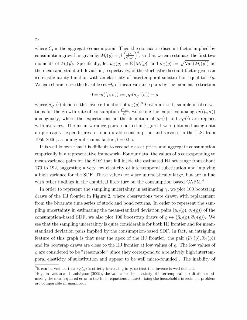
Figure 3 shows the 95% confidence region based on the LR statistic. By construction,

the LR confidence region covers most of the bootstrap draws below the HJ bounds.

However, it should also be noted that the confidence bound based on the LR statistic is

fairly tight relative to the boostrapped frontiers, and does not include any unnecessary

areas of the parameter space. Noting that the set Θe for the consumption-based SDF is

defined by a moment equality, we can also form a confidence band Re for Θe based on the

statistic Ln(θ) :=[mSDF (θ)

s(θ)

]2, noting that the asymptotic arguments in the derivations

for the (one-sided) LR statistic can be easily extended to the two-sided case if we replace

squared positive parts [·]2+ with the usual square, (·)2. The lower and upper bounds in

the following figures were constructed using separate estimates of the local standard de-

viation s((µ, σ)) based on the negative and positive deviations of m((µ, σ)), respectively

to improve the approximation. Critical values were obtained using the nonparametric

bootstrap.

Most importantly, the LR-based confidence region for the HJ set does not overlap

with the confidence set for the consumption-based SDF for “small” values of (in fact,

for any ∈ [0, 120]). The absence of overlap for the 95% regions implies the rejection of

any ∈ [0, 120] at 10% significance level. This is clear evidence against the benchmark

formulation of the consumption-based CAPM, and therefore an important empirical

conclusion. In what follows below we will show that the same empirical conclusion cannot

be reached for this example using less precise or non-invariant methods. Specifically, we

will show that if we use confidence regions based on either LR-statistic without precision

weighting, or Wald statistics without invariance/precision weighting, or regions based

on structural projection, we will not be able to reach the same empirical conclusion. So

invariance and precision considerations in construction of the confidence regions turn

out to be quite important for reaching sharp economic conclusions.

28

Figure 4 plots the 95% confidence region based on an unweighted LR statistic. Com-

paring Figure 3 and Figure 4 it can be seen that precision weighting plays a very impor-

tant role in delivering good confidence sets. Without precision weighting, the unweighted

LR statistic delivers a confidence region that includes implausible regions in the param-

eter space where the standard deviation of the discount factor is zero. Moreover, the

confidence region becomes too imprecise to reject the canonical model of the stochastic

discount factor.

Figure 6 plots the confidence region based on the Wald statistic with no invari-

ance/precision weighting, which is equivalent to a confidence region based on the di-

rected Hausdorff distance. Similar to Figure 4 the confidence set covers a large area of

the parameter space which is excluded from any bootstrap realization of the HJ set. The

shape of the confidence region based on the Wald statistic in Figure 6 seem counter-

intuitive because at first sight, as the confidence bounds do not appear to be a uniform

enlargement of the estimated frontier ∂Θ. However, this visual impression is only due

to the fact that the plot shows units of µ and σ at different scales. The observation

that the weighting and scaling of the different components of θ seem “unnatural” in this

particular graph emphasizes the potential problems associated with the non-invariance

of inference based on the unweighted Wald statistic.

Figure 5 plots the confidence region based on the weighted Wald statistic, where

weights induce first order invariance and similarity via precision weighting. This weight-

ing fixes the problem and generates a statistic that is (first-order) invariant to parameter

transformations. As a result, the confidence set looks very similar to weighted LR based

confidence set in Figure 3 in that it covers most of the bootstrap draws below the HJ

bounds and its shape reflects local sampling uncertainty in an adequate manner. This

practical evidence therefore emphasizes the importance of introducing invariance and

precision inducing weights in the Wald-based approach, which we had argued for theo-

retically in the previous sections.

Finally, in Figure 7 we compare our results to confidence regions from the structured

projection approach that is based on a confidence set for the point-identified parameters.

As described in section 2.5, we construct an elliptical joint 1 − α confidence region for

the quantity γ defined in equation (1.2) based on the quadratic form for the estimator

γ, T (γ) := (γ−γ)′var(γ)−1(γ−γ). For the diameter of this confidence ellipsoid we used

both a bootstrap and a chi-square approximation to the distribution of T (γ), which both

yield qualitatively similar results.

29

The 1−α confidence set for θ = (µ, σ) is obtained by projecting the 1−α confidence

region for γ onto Θ using the condition m(θ, γ) ≤ 0. We report the resulting confidence

set from the structured projection approach in Figure 7 together with the LR-based

confidence set proposed in this paper. The structured projection confidence set performs

quite poorly relative to the LR-based confidence set: in particular the latter is much

smaller and lies strictly inside the former. In fact, the precision of the confidence set

based on structured projection is poor enough to overturn the major empirical conclusion

that the consumption-based CAPM cannot be reconciled with small values of .

This should be expected since the projection confidence bounds are based on a confi-

dence set for the point-identified parameter that does not account for the specific shape

of the bounds as a function of γ. More specifically, the elliptical joint confidence set

for γ (which minimizes volume under joint normality of γ) guards us against deviations

from the true value in any direction in R3, but most of these deviations are irrelevant

for the bounds for θ, since these are only one-sided and the parameter space for θ is

only two-dimensional. The fact that the standard confidence set for γ treats all direc-

tions in the parameter space Γ symmetrically may be far from ideal for inference on the

(µ, σ)-frontier, since the bound on the standard deviation is a nonlinear function whose

derivative with respect to γ varies widely across different values of (µ, σ(µ)). Note that

for confidence sets for a point-identified parameter, by the delta method the effect of

nonlinearities is asymptotically negligible to first order. However when the object of

interest is a set with a nontrivial diameter, the resulting effect is of first order even for

large samples.

3.2. Bounds on the Elasticity of Labor Supply. In his meta-analysis, Chetty (2012)

reports point-wise confidence bounds for the structural Hicksian elasticity ε of labor

supply at the intensive margin for given values of the optimization friction δ. The

reported bounds result from the intersection of bounds of the form (1.4) from estimates

εj obtained from J empirical studies studies exploiting different natural experiments

varying the effective income tax ∆j log p, j = 1, . . . , J .

We apply the bootstrap procedure proposed in this paper to obtain joint confidence

sets for (δ, ε) based on the LR and Wald statistics. More specifically, we consider the

moments obtained from individual empirical elasticities εj

gOF,j((ε, δ)′) = gOF,j((ε, δ)

′, εj) :=(ε− εj)

2(∆j log p)2

8ε− δ.

30

These “raw” moments are then aggregated by a smooth function

m∗OF (ε, δ;λ) =

∑Jj=1

exp(λgOF,j(ε, δ))∑Jl=1 exp(λgOF,l(ε, δ))

gOF,j(ε, δ),

where λ ∈ R is a fixed, positive scalar. Note that as discussed in Section 2, this

transformation approximates the maximum of gOF,1(ε, δ), . . . , gOF,J(ε, δ) as λ → ∞,

but satisfies the smoothness conditions for our procedure for any finite value of λ > 0.

We use a parametric bootstrap to obtain the critical value k(1−α), where we approx-

imate the sampling distribution of the estimators for the respective elasticities by a joint

normal distribution centered around the estimates reported in Panel A of table 1 with

standard deviations equal to the respective standard errors and zero covariances. This

approach can be justified by an assumption that the studies were based on mutually

independent random samples from possibly different populations.

Figure 8 shows that the estimated bounds coincide with the set reported in Figure 8

of Chetty (2012) except for the use of the smoothed maximum function instead of the

intersection of (ε, δ)-sets which leads to a slightly wider set. The 95% confidence set

based on the LR statistic5 reported in Figure 9 is fairly narrow around the estimated

bound, and does not appear to differ very much from the the collections of confidence

intervals in Chetty (2012). Chetty presents confidence intervals that are pointwise with

respect to δ, that is for each fixed value of friction δ, the interval covers structural elas-

ticity ε with a prescribed probability. In contrast, our set estimator covers all plausible

values of (δ, ε) with a prescribed probability. Thus it simultaneously performs inference

on both structural elasticity ε and the friction amount δ. The LR confidence region is a

valid joint confidence set for (ε, δ) and not only point-wise in δ. Furthermore, it is not

conservative in that we assume a joint sampling distribution for the elasticity estimates

instead of constructing Frechet-Hoeffding bounds. The LR confidence region excludes

all points with δ ≤ 0.3%, so that an optimization friction of at least that size would

be needed to reconcile the different elasticities found in the studies considered in this

meta-analysis.

5 Note that for the LR statistic we used the standard error of the negative part of m∗(θ) as a weightingfunction which improves the local approximation due to the asymmetry of the distribution for smallvalues of . Note that for the N(0, s(θ)2) distribution, the standard deviation of the negative part isproportional to s(θ), so that this weighting scheme is asymptotically equivalent to weighting by the(inverse of the) local standard deviation of m∗(θ).

31

Finally, we also report a 95% confidence region based on the Wald statistic without

optimal re-weighting.6 As in the case of HJ bounds, the shape of the resulting confidence

set does not reflect the sampling variation in the estimated bounds, and the critical value

for the Wald statistic is determined by perturbations of the frontier at very low values

for ε. More importantly, in contrast to the LR-based region, the confidence set based

on the Wald statistic includes points with δ = 0, failing to reject that the empirical

elasticities can be reconciled in a model with no optimization frictions and changing one

of the main conclusions of the analysis. Using weighted W statistics instead fixes this

problem and gives a confidence set that is very similar to the LR-based confidence set;

we do not report this confidence set for brevity.

4. Conclusion

In this paper we provide new methods for inference on parameter sets and frontiers

that can be characterized by a smooth nonlinear inequality. The proposed procedures

are straightforward to implement computationally and have favorable statistical prop-

erties. By analyzing the geometric and statistical properties of different statistics, we

illustrate the importance of equivariance and similarity considerations for achieving tight

confidence regions. In particular, while local weighting is irrelevant for the statistical

properties of the estimated frontier, it matters greatly for the size and shape of confidence

sets. We also consider smoothed intersection bounds from multiple inequality restric-

tions, where we give an exact upper bound for the approximation error that depends

only on the smoothing parameter.

We illustrate the practical usefulness of these procedures in financial econometrics with

various classical examples from mean-variance analysis, including inference on Hansen-

Jagannathan mean-variance sets of admissible stochastic discount factors, Markowitz-

Fama mean-variance sets of admissible portfolios, and factor-based asset pricing. As a

second application, we consider Chetty (2012)’s joint bounds for the elasticity of labor

supply and an optimization friction. This example suggests a broader range of uses for

set inference in the context of possibly misspecified or incomplete economic models.

In both examples, using invariant or precision-weighted statistics is important for

maintaining major empirical conclusions that have been reached informally in prior

6In order to adjust for the differences in order of magnitude we constructed the Hausdorff-distancebased on the norm ‖(ε, δ)‖ =

√ε2 + 100 · δ2. Note that in the graph the confidence region looks poorly

centered around the estimated bound, but this optical impression is in fact due to the different scalingof the two axis and the difference in the slope of the frontier above and below its apex.

32

empirical work, e.g. the inability of large values of the elasticity of intertemporal substi-

tution to generate plausible distributions of stochastic discount factors, or the need for

nontrivial optimization frictions to reconcile estimated demand elasticities from different

settings. Therefore, the empirical examples illustrate our formal points about the ad-

vantages of inference based on a precision weighted metric that is invariant to parameter

transformations.

33

Appendix A. Proofs

Proof of Lemma 1. W.l.o.g., let maxj gj = g1 and rewrite

λ

(max

jgj −m(g1, . . . , gJ ;λ)

)=

∑Jj=1 expλ(gj − g1)λ(g1 − gj)∑J

j=1 expλ(gj − g1)

=

∑Jj=1 exp−hjhj∑Jj=1 exp−hj

,

where hj := λ(g1 − gj) ≥ 0. Clearly, this expression is nonnegative, and since h1 = 0,

the denominator is bounded from below by 1. Next note that the function

F (h2, . . . , hJ) :=

∑Jj=2 exp−hjhj

1 +∑J

j=2 exp−hj

is strictly quasi-concave on RJ−1+ , so that the usual first-order conditions for a local

extremum are sufficient for a global maximum. We can now verify that the first-order

conditions for maximization of F (h2, . . . , hJ) have the symmetric solution h2 = · · · =hJ = h∗ := 1 + W ∗ where W ∗ := W

(J−1e

). Note that by definition of the product

logarithm, W ∗ = J−1e

exp−W ∗ = (J − 1) exp−1−W ∗, so that

maxh2,...,hJ≥0

F (h1, . . . , hJ) ≡∑J

j=2 exp−h∗h∗

1 +∑J

j=2 exp−h∗=

(J − 1) exp−1−W ∗(1 +W ∗)

1 + (J − 1) exp−1−W ∗

=W ∗ + (J − 1) exp−1−W ∗W ∗

1 + (J − 1) exp−1 −W ∗ = W ∗ = W

(J − 1

e

)

Since λ (maxj gj −m(g1, . . . , gJ ;λ)) = F (λ(g1 − g2), . . . , λ(g1 − gJ)), we therefore have

that

supg1,...,gJ

λ

∣∣∣∣maxj

gj −m(g1, . . . , gJ ;λ)

∣∣∣∣ = suph2,...,hJ≥0

|F (h2, . . . , hJ)| = W

(J − 1

e

)

which establishes the conclusion.

Next, we will prove four lemmas which will be used to justify the local approximation

for the Wald statistic. We consider a (stochastic or deterministic) sequence of moment

functions mn(θ) := m(θ)− qn, where qn = op(1), and m(θ) satisfies Conditions R.1-R.2

from the main text, and the corresponding sequence of parameter sets Θn := θ ∈ Θ :

mn(θ) ≤ 0.

34

Lemma 2. Suppose the parameter space Θ is compact. Suppose that the gradient

∇θmn(θ) is bounded away from zero uniformly in θ and n = 1, 2, . . . , and Lipschitz-

continuous in θ with Lipschitz constant L < ∞. Also let θn be any sequence such that

θn approaches the boundary Θn, i.e. d(θn, ∂Θn) → 0. Then there exists δ > 0 such that

the projection of θn on Θn is unique for all such sequences whenever d(θn,Θn) < δ.

Proof: Suppose the statement wasn’t true. Then for some sequence θn, we could

construct a subsequence θk(n) such that there are (at least) two distinct projections of

θs(n) onto ∂Θn for each n. By compactness of Θ, θk(n) has a convergent sub-subsequence

θb(n) with limn θb(n) = θ0, say. Since by construction every member of θb(n) has two

distinct projections onto ∂Θn, we can inscribe a ball of radius rn := d(θb(n), ∂Θn) centered

at θb(n) into Θ/Θn such that this ball has at least two distinct points (θ∗1,b(n), θ∗2,b(n)) in

common with ∂Θn.

By properties of the projection, the radii of these balls corresponding to the projection

points, N(θ∗j,b(n)) := r−1n (θb(n)−θ∗j,b(n)) for j = 1, 2, are also normal vectors to the surface

∂Θn at θ∗1,b(n) and θ∗2,b(n), respectively. Note that, since the gradient ∇θmn(θ) is bounded

away from zero, we can w.l.o.g. normalize the length of the normal vectors of the surface

∂Θn to 1.

Note that the two points θ∗1,b(n), θ∗2,b(n) are equidistant to θb(n), and therefore lie on a

one dimensional sphere S1(rn, θb(n)) ⊂ Θ with center θb(n) and radius rn. The curve η(s)

corresponding to a sphere of radius r, where s is the arc length, has constant curvature

κ(s) ≡ 1rn, so that the normal vectors (with length normalized to one) N(θ∗j,b(n)) :=

r−1n (θb(n) − θ∗j,b(n)) for j = 1, 2 satisfy

‖N(θ∗2,b(n))−N(θ∗1,b(n))‖ & r−1n ‖θ∗2,b(n) − θ∗1,b(n)‖.

Since rn → 0, there is no upper bound on r−1n , so that N(θ) is not Lipschitz continuous.

However, the normal vector of ∂Θ0 at θ standardized to length 1 is given by

N(θ) := ‖∇θm(θ)‖−1∇θm(θ).

Condition R.2 implies that N(θ) is Lipschitz continuous in θ with a constant 1/δ < ∞,

which leads to a contradiction. Finally, note that since that Lipschitz constant L was

assumed to be uniform in γ, there exists δ := δ(L) > 0 such that projection is unique

whenever rn := d(θn,Θn) < δ along all sequences θn and mn(·)

35

Lemma 3. Suppose R.1 and R.2 hold, and let θn be a sequence such that d(θn,Θ0) →0. Define θn ≡ argminm(θ)≤0 ‖θn − θ‖2. Then θn is uniquely defined with probability

approaching 1, and satisfies d(θn,Θ0)p→ 0.

Proof of Lemma 3. For a given value of δ > 0, let η := minm(θ) : d(θ,Θ0) ≥ δ.By continuity of m(θ) and compactness of Θ, η > 0. By Condition R.1 supθ∈Θ0

m(θ) < η

w.p.a.1, and therefore d(θn,Θ0) < δ with probability approaching 1. Uniqueness follows

from Lemma 2, noting that the conclusion holds regardless of whether the sequence

mn(θ) is deterministic or stochastic

Lemma 4. Suppose Conditions R.1 and R.2 hold, and consider a sequence of parameter

values θn ∈ Θ such that θn → ∂Θ0. For a sequence qn = op(1) and Θn := θ ∈ Θ :

m(θ) ≤ qn, we have

√nd(θn, Θ0,δ) =

[‖∇θm(θn)‖−1(Gn(θn) +

√n(m(θn)− qn)) + op(1)

]+

In particular, for qn ≡ 0, we have

√nd(θn, Θ0,δ) =

[‖∇θm(θn)‖−1(Gn(θn) +

√nm(θn)) + op(1)

]+

Proof of Lemma 4. Without loss of generality, we only consider the case qn ≡ 0.

Note that for the general case, we can apply the same argument to the functions m(θ)−qn

and m(θ)− qn which inherit the properties R.1-R.2.

The projection of θn onto the set Θ0,δ := θ ∈ Θδ : m(θ) ≤ 0 is given by

θn := arg minθ′∈Θδ:m(θ′)≤0

‖θn − θ′‖2.

The Lagrangian for this constrained minimization problem is ‖θn − θ′‖2 + 2λm(θ′),

where the Kuhn-Tucker multiplier λ ≥ 0. Since δ > 0 is fixed and d(θn,Θ0) → 0 it follows

from Lemma 3 that θn is contained in the interior of Θδ with probability approaching

one. Hence for n large enough, the quantity θn can be taken to be an interior solution

of the saddle-point problem

(θn − θn) +∇θm(θn)λ = 0,

m(θn) = 0.

We can now use a mean-value expansion to obtain

(θn − θn) +∇θm(θn)λ = 0,

m(θn) +∇θm(θn)′(θn − θn) = 0,

36

for an intermediate value θn. By Lemma 3, ∇θm(θn) = ∇θm(θn)+op(1) and ∇θm(θn) =

∇θm(θn) + op(1). Hence, solving for (θn − θn) and applying the extended continuous

mapping theorem, we obtain

θn − θn = −[∇θm(θn)(∇θm(θn)′∇θm(θn))

−1 + op(1)]m(θn)

Now, since√n(m−m) = Gn = Op(1) in ℓ∞(Θδ), we obtain

√n(θn − θn) = −∇θm(θn)(∇θm(θn)

′∇θm(θn))−1(Gn(θn) +

√nm(θn)) + op(1)

Thus we have that

√nd(θn, Θ

δn) =

√n‖θn − θn‖1m(θn) > 0

=∣∣(∇θm(θn)

′∇θm(θn))−1/2(Gn(θn) +

√nm(θn)) + op(1)

∣∣ (A.1)

×1Gn(θn) +√nm(θn) > 0 + op(1) (A.2)

= [‖∇θm(θn)‖−1(Gn(θn) +√nm(θn)) + op(1)]+

(A.3)

which concludes the proof

A.1. Proof of Theorem 1. Part 1. (Limit law of Ln.) Let Gn =√n(m −m). We

first show that

Ln = supθ∈Θ0

[√nm(θ)/s(θ)

]2+

= supθ∈Θ0

[(Gn(θ) +

√nm(θ))/s(θ)

]2+

=(1) supθ∈∂Θ0

[(Gn(θ) +

√nm(θ))/s(θ) + op(1)

]2+

=(2) supθ∈∂Θ0

[(Gn(θ) +

√nm(θ))/s(θ) + op(1)

]2+

(3) supθ∈∂Θ0

[(G(θ) +

√nm(θ))/s(θ)

]2+,

where the steps follows from the following arguments.

To show step (1), note that

supθ∈Θ0

[(Gn(θ) +

√nm(θ))/s(θ)

]2+≥ sup

θ∈∂Θ0

[(Gn(θ) +

√nm(θ))/s(θ)

]2+.

So we need to show that with probability approaching 1,

supθ∈Θ0

[(Gn(θ) +

√nm(θ))/s(θ)

]2+≤ sup

θ∈∂Θ0

[(Gn(θ) +

√nm(θ))/s(θ) + op(1)

]2+.

37

To show this take a sequence θn ∈ Θ0 such that

supθ∈Θ0

[(Gn(θ) +

√nm(θ))/s(θ)

]2+=

[(Gn(θn) +

√nm(θn))/s(θn)

]2+,

where the supremum is attained by compactness of Θ0 and continuity hypotheses on

m,m, and s, and uniform positivity of s. Since supθ∈Θ |Gn| = Op(1), θn can be selected

to obey √nm(θn)/s(θn) = Op(1).

We now show that θn converges to ∂Θ0: fix κ > 0, and let

ζ(κ) := sup m(θ)/s(θ) : θ ∈ Θ0, d(θ, ∂Θ0) ≥ κ .

Next, note that Condition R.2 implies that m(θ) < 0 for each θ ∈ int Θ0: suppose this

wasn’t true, but that m(θ0) = 0 for some θ0 ∈ int Θ0. Then, since for θ ∈ Θ0 m(θ) ≤ 0,

θ0 represents a local maximum of m(·) in the interior of Θ0. Since m(θ) is differentiable,

this implies that ∇θm(θ0) = 0. However, Condition R.2 implies that ‖∇θm(θ)‖ > 0,

a contradiction. Therefore m(θ) < 0 for each θ ∈ int Θ0, so that by continuity and

compactness, ζ(κ) < 0.

By conditions R.1 and R.3, we have supθ∈Θ0|m(θ)/s(θ)−m(θ)/s(θ)| < −ζ with prob-

ability approaching one for any strictly negative value of ζ . Hence the supremum of√n [m(θ)/s(θ)]2+ for values θ ∈ Θ0 such that d(θ, ∂Θ0) ≥ κ is equal to zero with proba-

bility approaching one, so that the supremum over all of Θ0 is attained at a value of θ

such that d(θ, ∂Θ0) < κ. Since κ can be chosen arbitrarily close to zero, we can construct

a sequence of positive random variables κn = op(1) such that

d(θn, ∂Θ0) ≤ κn,

with probability approaching 1. We conclude that

supθ∈Θ0

[(Gn(θ) +

√nm(θ))/s(θ)

]2+

≤ supθ∈∂Θ0,θ+η∈Θ0,‖η‖≤κn

[(Gn(θ + η) +

√nm(θ + η))/s(θ + η)

]2+.

Using stochastic equicontinuity of Gn implied by R.1, the last quantity is equal to

supθ∈∂Θ0,θ+η∈Θ0,‖η‖≤κn

[(Gn(θ) +

√nm(θ + η))/s(θ + η) + op(1)

]2+,

38

for some op(1) term. Because√nm(θ+ η) ≤ 0 for θ+ η ∈ Θ0 and m(θ) = 0 for θ ∈ ∂Θ0,

we conclude that the last quantity is equal to

supθ∈∂Θ0

[(Gn(θ)/s(θ + η) + op(1)]2+ ,

for the same op(1) term. This verifies equality (1).

Equality (2) follows from using R.3 and that the fact that supθ∈Θ |Gn(θ)| = Op(1)

implied by R.1. Equality (3) follows from the application of R.1 and the Continuous

Mapping Theorem.

Part 2. (Limit Law of Wn). Recall that we define the set estimator Θ0,δ as

Θ0,δ :=θ ∈ Θδ : m(θ) ≤ 0

.

In analogy to part 1, we establish the conclusion by the following steps:√

Wn = supθ∈Θ0

√nd(θ, Θ0,δ)/w(θ) =(1) sup

θ∈∂Θ0

[(Gn(θ) +

√nm(θ))/w(θ) + op(1)

]+

=(2) supθ∈∂Θ0

[(Gn(θ) +

√nm(θ))/w(θ) + op(1)

]+

(3) supθ∈∂Θ0

[(G(θ) +

√nm(θ))/w(θ)

]+,

where steps (1)-(3) are proven as follows:

To establish step (1), we first show that

supθ∈Θ0

√nd(θ, Θ0,δ)/w(θ) = sup

Θn

√nd(θ, Θ0,δ)/w(θ) (A.4)

holds with probability approaching 1, where

Θn = θ ∈ Θ0 : d(θ, ∂Θ0)/w(θ) ≤ κn,

and κn is some sequence of positive random variables converging to zero in probability,

κn = op(1). Note that right hand side of (A.4) is less than or equal to the left hand side

of (A.4) by construction, so we only need to show that w.p.a.1, the right hand side can

not be less. To this end, fix some κ > 0 and note that using the same line of reasoning

as for part 1, we have

ζ(κ) := supm(θ) : θ ∈ Θ0, d(θ, ∂Θ0) ≥ κ < 0.

39

Furthermore, for every ζ < 0 we have that with probability approaching 1, supθ∈Θ |m(θ)−m(θ)| < −ζ , and therefore each θ ∈ Θ0 with d(θ, ∂Θ0) ≥ κ is included in Θ0,δ. In that

event, we can only have d(θ, Θ0,δ) > 0 for values of θ within a distance κ of the boundary

∂Θ0. Since κ can be chosen arbitrarily small, we can choose a sequence κn = o(1) such

that the right-hand side in (A.4) holds with probability converging to one.

Next, let θn be a sequence such that

supθ∈Θ0

√nd(θ, Θ0,δ)/w(θ) =

√nd(θn, Θ0,δ)/w(θn).

Note that since d(θ, Θ0,δ) and w(θ) are continuous functions of θ, w(θ) is bounded away

from zero with probability approaching 1, so that since Θ0 is compact, the supremum

is attained with probability approaching 1. Since δ > 0 is fixed and by Lemma 3 with

probability approaching 1, we have d(θn, θn)/w(θ) < δ, so that θn is contained in the

interior of Θδ w.p.a.1.

It follows from Lemma 4 that

√nd(θn, Θ0,δ) =

[‖∇θm(θn)‖−1(Gn(θn) +

√nm(θn)) + op(1)

]+

Hence, dividing by w(θ) and using stochastic equicontinuity of Gn(θ), we can follow the

same line of reasoning as in part 1 to obtain that with probability approaching 1,

supθ∈Θ0

√nd(θ, Θ0,δ)/w(θ) ≤ sup

θ∈∂Θ0,θ+η∈Θ0,‖η‖≤κn

[Gn(θ) +

√nm(θ + η)

‖∇θm(θ)‖w(θ + η)+ op(1)

]

+

Noting again that√nm(θ + η) ≤ 0 for θ + η ∈ Θ0, we can bound the expression by

supθ∈Θ0

√nd(θ, Θ0,δ)/w(θ) ≤ sup

θ∈∂Θ0,θ+η∈Θ0,‖η‖≤κn

[Gn(θ)

‖∇θm(θ)‖w(θ + η)+ op(1)

]

+

where again the op(1) term is the same as in the first inequality.

Therefore, we can use uniform convergence of the weighting function w to w from

Condition R.3 and the continuous mapping theorem to obtain

Wn supθ∈∂Θ0

[(‖∇θm(θ)‖w(θ))−1

G(θ)]2+

(A.5)

where the intermediate steps are analogous to equalities (2) and (3) in the proof for Ln.

Part 3. (Continuity of the Limit Distributions). The continuity of the distribution

function L on (0,∞) follows from Davydov et al. (1998) and from the assumption that

40

the covariance function of G is non-degenerate, i.e. infθ∈ΘVar(G(θ)) > 0. The proba-

bility that L is greater than zero is equal to the probability that maxj supθ∈Θ Gj(θ) > 0,

which is greater than the probability that Gj′(θ′) > 0 for some fixed j′ and θ′, but

the latter is equal to 1/2. Therefore the claim follows. The claim of continuity of the

distribution function of W on (0,∞) follows similarly.

A.2. Proof of Corollary 1. This corollary immediately follows from the assumed con-

ditions and from the comments given in the main text preceding the statement of Corol-

lary 1.

A.3. Proof of Theorem 2. We have that P[Θ0 ⊆ RLR] = P[Ln ≤ k(1 − α)] by the

construction of the confidence region. We then have that for any α < 1/2 that k(1−α)

is a continuity point of the distribution function of L, so that for any sufficiently small ǫ

P[Ln ≤ k(1− α)] ≤ P[Ln ≤ k(1− α) + ǫ] + o(1) → P[L ≤ k(1− α) + ǫ],

P[Ln ≤ k(1− α)] ≥ P[Ln ≤ k(1− α)− ǫ]− o(1) → P[L ≤ k(1− α)− ǫ].

Since we can set ǫ as small as we like and k(1−α) is a continuity point of the distribution

function of L, we have that

P[Ln ≤ k(1− α)] → P[L ≤ k(1− α)] = (1− α).

We can conclude similarly for the W-statistic Wn. .

A.4. Proof of Theorem 3. We will give the proof only for confidence regions based

on the LR statistic. The arguments for the Wald-type confidence sets are completely

analogous. Let δn be a null sequence where δn > 0 for all n and√nδn → ∞. In order to

show convergence with respect to Hausdorff distance, we establish that with probability

approaching 1, (a) RLR ⊂ Θδn0 , and (b) Θ0 ⊂ Rδn

LR, where for δ > 0, Aδ := x ∈ Rk :

d(x,A) < δ denotes the δ-expansion of a set A in Rk.

To prove statement (a), consider a sequence θn ∈ Θ\Θδn0 . We have to show that

θn /∈ RLR w.p.a.1 as n increases: For any fixed δ > 0, let η := infθ:d(θ,Θ0)≥δ m(θ).

Since Θ is compact and m(θ) is continuous by R.2, it follows from the definition of Θ0

that η > 0. Hence, along any sequence θn such that d(θn,Θ0) ≥ δ for all n, we have√nm(θn) → ∞. Since θ ∈ RLR if and only if for the critical value k LRn ≤ k, where k

is tight for any n large enough, it follows that θn /∈ RLR w.p.a.1. Hence we can restrict

our attention to (sub-) sequences for which d(θn,Θ0) → 0.

41

Now suppose that d(θn,Θ0) → 0, and√nd(θn,Θ0) → ∞. Let θ∗n be the projection of

θn onto ∂Θ0, where θ∗n need not converge to a particular point. Then using the same

steps as in the proof of Lemma 4 it follows from a mean-value expansion of m(θ) around

θn and continuity of the gradient ∇θm(θ) that√nm(θn) → ∞. Hence the LR-statistic

diverges to infinity, and θn /∈ RLR w.p.a.1.

It remains to check claim (b), namely that Θ0 ⊂ RδnLR. To this end, consider a sequence

θn ∈ Θ0, and let qn = s(θ)

√k(1− α)/n. Also define θn ≡ argminm(θ)≤qn ‖θn − θ‖2, so

that d(θn, Θ0,δ) = ‖θn − θn‖. Now note that Lemma 3 implies that d(θn,Θ0)p→ 0, so

that we can apply Lemma 4 to obtain

√nd(θn, θn) = [‖∇θm(θn)‖−1(Gn(θn) +

√n(m(θn)− qn)) + op(1)]+

By assumption R.2, the norm of ∇θm(θn) is bounded away from zero, and Gn(θn) is

stochastically bounded by Condition R.1. Since s(θ) and k are stochastically bounded

by R.3,√nqn is also stochastically bounded.

Noting that m(θn) ≤ 0, it follows that√n(θn − θn) = Op(1). Therefore

supθ∈Θ0

√nd(θ, RLR) = Op(1)

so that for any sequence δn such that√nδn → ∞, we have d(θ, RLR)/δn → 0. Hence

Θ0 ⊂ RδnLR w.p.a.1, which concludes the proof

A.5. Proof of Corollary 2. This corollary immediately follows from the assumed con-

ditions and Corollary 1.

A.6. Proof of Theorem 4. In what follows let A denote an absolute positive constant.

We have by definition of the Kantarovich-Rubenstein metric that

EQV ∗ [ϕ(V∗)]− EQV

[ϕ(V )] = op(1) uniformly in ϕ ∈ BL1(C(Θ)).

This implies that

EQV ∗ [ϕ([V∗]2+)]− EQV

[ϕ([V ]2+)] = op(1) uniformly in ϕ ∈ BL1(C(Θ)),

since the composition ϕ [·]2+ ∈ A ·BL1(C(Θ)) for ϕ ∈ BL1(C(Θ)). This further implies

that

EQV ∗ [ϕ′(sup

Rn

[V ∗]2+)]− EQV[ϕ′(sup

Rn

[V ]2+)] = op(1) uniformly in ϕ′ ∈ BL1(R),

42

since the composition ϕ′(supRn[·]2+) ∈ A · BL1(C(Θ)) for ϕ′ ∈ BL1(R) and Rn denoting

any sequence of closed non-empty subsets in Θ. Therefore, by the Extended Continuous

Mapping Theorem,

EQV ∗ [ϕ′(sup

∂Θ0

[V ∗]2+)]− EQV[ϕ′(sup

∂Θ0

[V ]2+)] = op(1) uniformly in ϕ′ ∈ BL1(R).

(Note that here we compute expectations over V ∗ and V taking ∂Θ0 as given; note that

our bootstrap method treats ∂Θ0 as fixed.) Also note that any sequence of sets Rn

converging to a set R, we have that

|EQV[ϕ′(sup

Rn

[V ]2+)− ϕ′(supR

[V ]2+)]|

≤ EQV[| sup

Rn

[V ]2+ − supR

[V ]2+| ∧ 1] = op(1) uniformly in ϕ′ ∈ BL1(R),

since

supRn

[V ]2+ − supR

[V ]2+ = op(1)

by stochastic equicontinuity of the process V . Since by Condition R.1-R.3 and Theorem

3, ∂Θ0 converges to ∂Θ0 in the Hausdorff distance, we have by the Extended Continuous

Mapping Theorem:

|EQV[ϕ′(sup

∂Θ0

[V ]2+)− ϕ′(sup∂Θ0

[V ]2+)]| = op(1) uniformly in ϕ′ ∈ BL1(R),

where QV computes the expectation over V , treating ∂Θ0 as fixed.

Combining the steps above, we conclude by the triangle inequality that:

|EQV ∗[ϕ′(sup

∂Θ0

[V ∗]2+)− ϕ′(sup∂Θ0

[V ]2+)]| = op(1) uniformly in ϕ′ ∈ BL1(R),

which is the same as

ρK(QS∗ ,QS) = op(1).

(Note that the bootstrap random variable S∗ is computed having fixed ∂Θ0.)

It is known that the convergence ρK(QSn ,QS) = o(1), for any sequence of laws QSn

of a sequence of random variables Sn defined on probability space (Ω′,F ′, Pn) implies

the convergence of the distribution function

PrQSn[Sn ≤ s] = PrQS

[S ≤ s] + o(1),

43

at each continuity point (0,∞) of the mapping s 7→ Pr[S ≤ s] and also convergence of

quantile functions

infs : PrQSn[Sn ≤ s] ≥ p = infs : PrQS

[S ≤ s] ≥ p+ o(1)

at each continuity point p of the mapping s 7→ infs : PrQS[S ≤ s] ≥ p. Recall from

Theorem 1 that the set of continuity points necessarily includes the region (0, 1/2).

By the Extended Continuous Mapping Theorem (see e.g. Theorem 18.11 in van der Vaart

(1998)) we conclude that since ρK(QS∗ ,QS) = op(1), we obtain the convergence in prob-

ability of the distribution function

PrQS∗ [S∗ ≤ s] = PrQS[S ≤ s] + op(1),

at each continuity point (0,∞) of the mapping s 7→ Pr[S ≤ s] and also convergence in

probability of the quantile functions

infs : PrQS∗ [S∗ ≤ s] ≥ p = infs : PrQS[S ≤ s] ≥ p+ op(1),

at each continuity point p of the mapping s 7→ infs : PrQS[S ≤ s] ≥ p.

A.7. Proof of Proposition 1. First note that γHJ and γMF are continuous, differ-

entiable functions of the elements in v,Σ, and B, so that C.1 follows from a CLT for

v, vec(Σ), vec(B) and the delta-rule.

Next, we check Condition C.2 for the HJ bounds. Recall that the moment function

defining the HJ bound was given by

mHJ((µ, σ)′, γHJ) =

√Svvµ2 − 2Sv1µ+ S11 − σ

with Svv, Sv1, S11 as defined in section 1.

Since the derivative of mHJ ((µ, σ)′, γHJ) with respect to σ is equal to minus one, the

lower bound on the norm of the gradient holds for all θ ∈ Θ. Also, since the eigenvalues

of Σ are bounded away from zero, and the elements of |v| are bounded, |Svv| and |Sv1|are also bounded. Furthermore, we can easily verify that

Svvµ2 − 2Sv1µ+ S11 ≥

SvvS11 − S2v1

Svv.

for all values of µ. Now, since the eigenvalues of Σ−1 are bounded away from zero, and

v′v1′N1N − (1′Nv)2 is bounded from below by a positive constant by assumption, we can

also bound Svvµ2 − 2Sv1µ+ S11 away from zero.

44

Noting that the parameter space Θδ ×Γ is compact, it follows that the second deriva-

tives ofm(HJ)(θ, γHJ) with respect to γHJ and θ, respectively, are bounded. In particular,

this implies Lipschitz continuity of the gradients ∇γm(HJ)(θ, γHJ) and ∇θm

(HJ)(θ, γHJ).

The arguments for the moment function mMF (θ, γMF ) for the MF mean-variance set

for asset portfolios are completely analogous.

A.8. Proof of Corollary 3. First note that by Proposition 1, Conditions C.1 and C.2

hold. Hence, in order to prove this corollary it suffices to show that

ρK(Qt′Z∗ ,Qt′Z ;C(Θ)) = op(1).

Without loss of generality we can take supθ ‖t(θ)‖ ≤ 1 and supθ ‖t(θ)‖ ≤ 1. The claim

will follow from

ρK(Qt′Z∗ ,Qt′Z ;C(Θ)) ≤ ρK(Qt′Z∗ ,Qt′Z ;C(Θ)) + ρK(Qt′Z ,Qt′Z ;C(Θ)) = op(1).

That ρK(Qt′Z∗,Qt′Z ;C(Θ)) = op(1) follows immediately from ρK(QZ∗ ,QZ) = op(1) and

ϕ(t′·) ∈ BL1(Rk). Indeed,

|ϕ(t(θ)′z(θ))− ϕ(t(θ)′z(θ))| ≤ supθ

|t(θ)′(z(θ)− z(θ))| ∧ 2

≤ [(supθ

‖t(θ)‖ supθ

‖z(θ)− z(θ)‖) ∧ 2]

≤ [supθ

‖z(θ)− z(θ)‖ ∧ 2].

That ρK(Qt′Z ,Qt′Z ;C(Θ)) = op(1) follows because uniformly in ϕ ∈ BL1(C(Θ))

|EQZ[ϕ(t′Z)]− ϕ(t′Z)| ≤ EQZ

[supθ

|(t(θ)− t(θ))′Z(θ)| ∧ 2]

≤ EQZ[sup

θ‖t(θ)− t(θ)‖ sup

θ‖Z(θ)‖ ∧ 2] = op(1),

where EQZcomputes the expectation over Z, treating t as fixed.

A.9. Proof of Proposition 3. For the LR-type statistic, it is sufficient to notice that

Ln(θ; η) = Ln(η−1(η(θ))) =

√nmn(θ)s(θ)

, and therefore only depends only on quantities

evaluated at θ. Hence,

Ln = supθ∈Θ0

Ln(θ) = supη∈η(Θ0)

Ln(η−1(η)),

and φLn(θ; η) is invariant with respect to parameter transformations. Asymptotic simi-

larity follows from Condition R.1 and the continuous mapping theorem.

45

Next, define H0,δ = η ∈ η(Θδ) : m(η) ≤ 0, noting that H0,δ = η(Θ0,δ). We now

distinguish three cases regarding the limit point of the sequence θn: (1) θ0 ∈ int Θ0,

the interior of Θ0, (2) θ ∈ Θ/Θ0, and (3) θ ∈ ∂Θ0.

Since the weighting functions w(θ; η) were assumed to satisfy Condition R.3, Theorem

3 implies that in case (1), φWn(θ; η) → 0 for all values of η, including the identity

transformation, so that by continuity of Wn(θ; η) in θ, we have

limn→∞

P(φWn(θn; η) 6= φWn(θn; η))

≤ max limn→∞

P (φWn(θ0; η) = 1), limn→∞

P (φWn(θ0) = 1) = 0.

Similarly, in case (2), we have

limn→∞

P(φWn(θn; η) 6= φWn(θn; η))

≤ max limn→∞

P (φWn(θ0; η) = 0), limn→∞

P (φWn(θ0) = 0) = 0.

Finally, consider the third case in which θ0 ∈ ∂Θ0: Using the expansion in Lemma 4, we

obtain that

Wn(θn; η) =

[d(η(θn), H0,δ)

w(θn; η)

]2

=

[d(η(θn), η(Θ0,δ))

w(θn; η)

]2

=

[Gn(θn) +

√nm(θn)

‖∇ηmη(θn; η)‖w(θn; η)+ oP(1)

]2

+

. (A.6)

Now suppose we split the sequence θn into three (possibly trivial) subsequences θqn, θrn ,

and θsn , respectively, such that√nm(θqn) = O(1),

√nm(θrn) → ∞, and

√nm(θsn) →

−∞. We can now analyze the behavior of φWn(·) separately along each of these subse-

quences. By Theorem 3,

limn→∞

P(φWrn(θrn ; η) = 0) = limn→∞

P(φWsn(θsn ; η) = 1) = 0

for all η, so that by the same arguments as before, the test is asymptotically invariant

along these subsequences.

Finally, consider the sequence θqn : if w(θ; η) = b(θ)‖∇ηm(η(θ))‖ + op(1), the expansion in

(A.6) together with the continuous mapping theorem implies that along the subsequence

46

θqn ,

Wqn(θqn; η) =

[Gn(θqn) +

√qnm(θqn)

b(θqn)+ op(1 +

√qnm(θqn))

]2

+

=

[Gn(θqn) +

√qnm(θqn)

b(θqn)+ op(1)

]2

+

.

so that the leading term of this expression is a function of θ which does not depend on

η.

Now note that for θ ∈ ∂Θ0 we have m(θ) = 0, so that by this expansion and stochastic

equicontinuity of G(θ) we have

Wn(η) := supθ∈∂Θ0

Wn(θ; η) W := supθ∈∂Θ0

[G(θ)

b(θ)

]2

+

where the limit does not depend on η. It follows that kWη(1− α) = kW (1−α) for all η,

so that φWn(θ; η) is asymptotically invariant along θqn with respect to transformations

η ∈ H∗, which establishes the second conclusion.

To establish the last claim, consider the Wald statistic in (2.4) with weighting function

w(θ) = s(θ)‖∇θm(θ)‖ + op(1). By Condition R.1 and the approximation in (A.5), Wn(θ)

converges in distribution to max0, Z2, where Z ∼ N(0, 1), for all values of θ ∈ ∂Θ0

and is therefore asymptotically pivotal on the boundary of Θ0. Hence for any fixed

critical level k, the limit limn→∞ P (Wn(θ) > k) is constant across all values of θ ∈ ∂Θ0

for any value k.

References

Beresteanu, A. and Molinari, F. (2008). Asymptotic properties for a class of partially

identified models. Econometrica.

Bohrer, R. (1973). An optimality property of Scheffe bounds. Annals of Statistics.

Britten-Jones, M. (1999). The sampling error in estimates of mean-variance efficient

portfolio weights. Journal of Finance.

Casella, G. and Strawderman, W. (1980). Confidence bands for linear regression with

restricted predictor variables. JASA.

Chernozhukov, V., Hong, H., and Tamer, E. (2007). Estimation and confidence regions

for parameter sets in econometric models. Econometrica.

Chetty, R. (2012). Bounds on elasticities with optimization frictions: A synthesis of

micro and macro evidence on labor supply. Econometrica.

47

Cochrane, J. H. (2005). Asset Pricing. Princeton University Press.

Critchley, F., Marriott, P., and Salmon, M. (1996). On the differential geometry of the

wald test with nonlinear restrictions. Econometrica.

Davydov, Y., Lifshits, M., and Smorodina, N. (1998). Local Properties of Distributions

of Stochastic Functionals. American Mathematical Society, Providence, RI.

Fama, E. (1996). Multifactor portfolio efficiency and multifactor asset pricing. The

Journal of Financial and Quantitative Analysis.

Gibbons, M., Ross, S., and Shanken, J. (1989). A test on the efficiency of a given

portfolio. Econometrica.

Hansen, L. P. and Jagannathan, R. (1991). Implications of security market data for

models of dynamic economies. The Journal of Political Economy.

Hansen, L. P. and Singleton, K. (1982). Generalized instrumental variables estimation

of nonlinear rational expectations models. Econometrica.

Kaido, H. and Santos, A. (2011). Asymptotically efficient estimation of models defined

by convex moment inequalities. working paper, BU and UCSD.

Lehmann, E. and Romano, J. (2005). Testing Statistical Hypotheses. Springer.

Lettau, M. and Ludvigson, S. (2009). Euler equation errors. Review of Economic Dy-

namics.

Ludvigson, S. (2012). Advances in consumption-based asset pricing: Empirical tests. in:

George M. Constantinides and Milton Harris and Rene M. Stulz (eds.), Handbook of

the Economics of Finance, vol. 2.

Markowitz, H. (1952). Portfolio selection. The Journal of Finance.

Molchanov, I. S. (1998). A limit theorem for solutions of inequalities. Scandinavian

Journal of Statistics.

Naiman, D. (1984). Optimal simultaneous confidence bounds. Annals of Statistics.

Penaranda, F. and Sentana, E. (2010). Spanning tests in return and stochastic dis-

count factor mean-variance frontiers: A unifying approach. working paper, UPF and

CEMFI.

Politis, D. N. and Romano, J. P. (1994). Large sample confidence regions based on

subsamples under minimal assumptions. The Annals of Statistics.

Scheffe, H. (1953). A method for judging all contrasts in the analysis of variance.

Biometrika.

Sentana, E. (2009). The econometrics of mean-variance efficiency tests: a survey. Econo-

metrics Journal.

48

van der Vaart, A. W. (1998). Asymptotic Statistics. Cambridge University Press.

van der Vaart, A. W. and Wellner, J. A. (1996). Weak Convergence and Empirical

Processes. Springer-Verlag New York.

49

0.4 0.5 0.6 0.7 0.8 0.9 1 1.1 1.20

1

2

3

4

5

6

mean

sta

nd

ard

de

via

tio

n

0 10 20

40 60

100

120

140

160

180

190

HJ FrontierSDF implied by Aggregate Consumption

Figure 1. Estimated HJ Bounds with Stochastic Discount Factors im-plied by CRRA preferences, data labels represent values for the IES

0.4 0.5 0.6 0.7 0.8 0.9 1 1.1 1.20

1

2

3

4

5

6

mean

sta

nd

ard

de

via

tio

n

0 10 20

40 60

100

120

140

160

180

190

Original FrontierSDF implied by Aggregate Consumption

Figure 2. Estimated HJ Bounds, Mean-Standard deviation pairs basedon Consumption SDF, and Bootstrap Draws

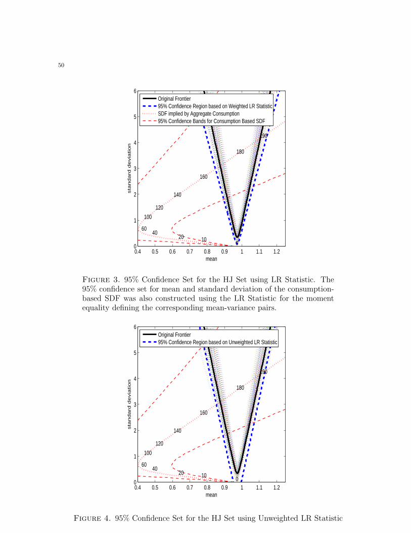
50

0.4 0.5 0.6 0.7 0.8 0.9 1 1.1 1.20

1

2

3

4

5

6

mean

sta

nd

ard

de

via

tio

n

0 10 20

40 60

100

120

140

160

180

190

Original Frontier95% Confidence Region based on Weighted LR StatisticSDF implied by Aggregate Consumption95% Confidence Bands for Consumption Based SDF

Figure 3. 95% Confidence Set for the HJ Set using LR Statistic. The95% confidence set for mean and standard deviation of the consumption-based SDF was also constructed using the LR Statistic for the momentequality defining the corresponding mean-variance pairs.

0.4 0.5 0.6 0.7 0.8 0.9 1 1.1 1.20

1

2

3

4

5

6

mean

sta

nd

ard

de

via

tio

n

0 10 20

40 60

100

120

140

160

180

190

Original Frontier95% Confidence Region based on Unweighted LR Statistic

Figure 4. 95% Confidence Set for the HJ Set using Unweighted LR Statistic

51

0.4 0.5 0.6 0.7 0.8 0.9 1 1.1 1.20

1

2

3

4

5

6

sta

nd

ard

de

via

tio

n

0 10 20

40 60

100

120

140

160

180

190

Original Frontier95% Confidence Region using Weighted W−Statistic

Figure 5. 95% Confidence Set for the HJ Set using Weighted W Statistic

0.4 0.5 0.6 0.7 0.8 0.9 1 1.1 1.20

1

2

3

4

5

6

mean

sta

nd

ard

de

via

tio

n

0 10 20

40 60

100

120

140

160

180

190

Original Frontier95% Confidence Set using Unweighted W−Statistic

Figure 6. 95% Confidence Set for the HJ Set using Unweighted W Statis-tic (directed Hausdorff Distance)

52

0.4 0.5 0.6 0.7 0.8 0.9 1 1.1 1.20

1

2

3

4

5

6

mean

sta

nd

ard

de

via

tio

n

0 10 20

40 60

100

120

140

160

180

190

Original Frontier95% Confidence Set based on Weighted LR Statistic95% Confidence Set based on Projection

Figure 7. 95% Confidence Sets for the HJ Set using Weighted LR Statis-tic and Projection Approach

0 0.01 0.02 0.03 0.04 0.050

0.5

1

1.5

ela

sticity

delta

Smoothed Intersection BoundOriginal Bounds

Figure 8. Bounds on Structural Labor Supply Elasticity based on Esti-mates from Different Studies, and their Smoothed Intersection Bound

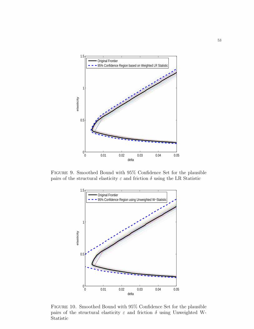
53

0 0.01 0.02 0.03 0.04 0.050

0.5

1

1.5

ela

sticity

delta

Original Frontier95% Confidence Region based on Weighted LR Statistic

Figure 9. Smoothed Bound with 95% Confidence Set for the plausiblepairs of the structural elasticity ε and friction δ using the LR Statistic

0 0.01 0.02 0.03 0.04 0.050

0.5

1

1.5

delta

ela

sticity

Original Frontier95% Confidence Region using Unweighted W−Statistic

Figure 10. Smoothed Bound with 95% Confidence Set for the plausiblepairs of the structural elasticity ε and friction δ using Unweighted W-Statistic