INFERENCE AND PARAMETER ESTIMATION IN bycagatayyildiz.github.io/pdf/msc_thesis.pdf · INFERENCE AND...

INFERENCE AND PARAMETER ESTIMATION IN

BAYESIAN CHANGE POINT MODELS

by

Cagatay Yıldız

B.S., Computer Engineering, Bogazici University, 2014

Submitted to the Institute for Graduate Studies in

Science and Engineering in partial fulfillment of

the requirements for the degree of

Master of Science

Graduate Program in Computer Engineering

Bogazici University

2017

ii



APPROVED BY:

Assoc. Prof. Ali Taylan Cemgil . . . . . . . . . . . . . . . . . . .

(Thesis Supervisor)

Assoc. Prof. Burak Acar . . . . . . . . . . . . . . . . . . .

Assist. Prof. Umut Simsekli . . . . . . . . . . . . . . . . . . .

DATE OF APPROVAL: 28.07.2017

iii

ACKNOWLEDGEMENTS

First and foremost, I would like to thank my advisor, Dr. Ali Taylan Cemgil, for

his assistance and patience. I feel truly privileged to study under his supervision. Also,

I thank Prof. Bulent Sankur for his guidance through the years. He has been, and will

be, a source of inspiration for me. Prof. Haluk Bingol was also very helpful towards

the end of my thesis, for which I am very grateful.

I have spent amazing years in my graduate study. Sharing the same office with

Taha Yusuf Ceritli and Barıs Kurt has always been fantastic, and will definitely be

missed! Hazal Koptagel, Beyza Ermis, Barıs Evrim Demiroz, Orhan ‘Abi’ Sonmez and

all other members of PILAB, many thanks for your support, academic discussions and

nice coffee breaks. Our lovely Department Chair Prof. Cem Ersoy, those cookies will

always be remembered.

I have been fortunate enough to meet wonderful people at Bogazici. It is not

possible to mention everyone here, but I would like to thank Betul Uysal, Seray Yuksel,

Berkant Kepez and Emre Erdogan for letting me share all the happiness and stress of

my graduate years, motivating nerdy talks and NBA chit-chats.

I would like to express my deepest gratitude to my beloved family, to whom this

thesis is dedicated. I have felt their endless love and wholehearted support throughout

my life. They made me -and everything I achieved- possible.

Finally, I would like thank the Scientific and Technological Research Council of

Turkey (TUBITAK). This thesis has been supported by the M.Sc. scholarship (2211)

from TUBITAK.

iv

ABSTRACT



In this work, we present a Bayesian change point model that identifies the time

points at which a time series undergoes abrupt changes. Our model is a hierarchical

hidden Markov model that treats the change points and the dynamics of the data

stream as latent variables. We describe a generic generative model, forward-backward

recursions for exact inference and an expectation-maximization algorithm for hyper-

parameter learning. The model specifications discussed here can sense the changes in

the state of the observed system as well as in the intensity and/or the ratio of the

features. In addition to investigating the change point algorithm in generic notation,

we also give an in-depth analysis and appropriate implementation of a particular model

specification, namely, Dirichlet-Multinomial model.

We present a novel application of the model: Distributed Denial of Service (DDoS)

attack detection in Session Initiation Protocol (SIP) networks. In order to generate

DDoS attack data, we build a network monitoring unit and a probabilistic SIP network

simulation tool that initiates real-time SIP calls between a number of agents. Using

a set of features extracted from target computer’s network connection and resource

usage statistics, we show that our model is able to detect a variety of DDoS attacks in

real time with high accuracy and low false-positive rates.

v

OZET

BAYESCI DEGISIM NOKTASI MODELLERINDE

CIKARIM VE PARAMETRE KESTIRIMI

Bu calısmada, zaman serilerindeki ani degisimlerin tespiti icin kullanılabilecek

bir Bayesci degisim noktası modelini sunuyoruz. Bu model, degisim noktalarını ve veri

dinamigini saklı degiskenler olarak temsil eden bir cok katmanlı saklı Markov modelidir.

Calısmamızda genel bir uretec modeli, cıkarım yapmak icin kullanılan ileri-geri yonlu

algoritmayı ve parametre kestirimi icin beklenti enyukseltme algoritmasını anlatıyoruz.

Modelin inceledigimiz dort ozel hali, gozlemlenen sistemin durumunda ve ozniteliklerin

yogunluk ve/veya oranında meydana gelen degisiklikleri tespit edebilmektedir. Modelin

genel halinin incelemesinin yanı sıra, ozel hallerinden birinin -Dirichlet-Multinomial

modeli- cozumlemesini yapıp nasıl gerceklestirilmesi gerektigini acıklıyoruz.

Modelin ozgun bir uygulaması olarak Oturum Baslatma Protokolu (SIP) aglarında

Dagıtık Hizmet Engelleme (DDoS) saldırısı tespiti problemini inceledik. DDoS saldırı

verisi uretmek icin bir ag izleme unitesi ve belirli sayıda kullanıcı arasında gercek za-

manlı SIP aramaları ureten bir olasılıksal SIP agı benzetim sistemi gelistirdik. Saldırılan

bilgisayarın ag baglantısından ve kaynak kullanım istatistiklerinden cıkardıgımız bir

veri kumesi uzerinde yaptıgımız deneylerde farklı niteliklere sahip bircok DDoS saldısını

gercek zamanlı olarak, yuksek dogruluk ve dusuk yanlıs kabul hatası oranlarıyla tespit

edebildigimizi gozlemledik.

vi

TABLE OF CONTENTS

ACKNOWLEDGEMENTS . . . . . . . . . . . . . . . . . . . . . . . . . . . . . iii

ABSTRACT . . . . . . . . . . . . . . . . . . . . . . . . . . . . . . . . . . . . . iv

OZET . . . . . . . . . . . . . . . . . . . . . . . . . . . . . . . . . . . . . . . . . v

LIST OF FIGURES . . . . . . . . . . . . . . . . . . . . . . . . . . . . . . . . . viii

LIST OF TABLES . . . . . . . . . . . . . . . . . . . . . . . . . . . . . . . . . . x

LIST OF SYMBOLS . . . . . . . . . . . . . . . . . . . . . . . . . . . . . . . . . xi

LIST OF ACRONYMS/ABBREVIATIONS . . . . . . . . . . . . . . . . . . . . xiii

1. INTRODUCTION . . . . . . . . . . . . . . . . . . . . . . . . . . . . . . . . 1

1.1. Related Work . . . . . . . . . . . . . . . . . . . . . . . . . . . . . . . . 2

1.2. Scope of the Thesis . . . . . . . . . . . . . . . . . . . . . . . . . . . . . 3

1.3. Organization of the Thesis . . . . . . . . . . . . . . . . . . . . . . . . . 4

2. THEORETICAL BACKGROUND . . . . . . . . . . . . . . . . . . . . . . . 5

2.1. Time Series Models . . . . . . . . . . . . . . . . . . . . . . . . . . . . . 5

2.1.1. Markov Model . . . . . . . . . . . . . . . . . . . . . . . . . . . . 5

2.1.2. Hidden Markov Model . . . . . . . . . . . . . . . . . . . . . . . 6

2.2. Parameter Estimation in Latent Variable Models . . . . . . . . . . . . 8

2.3. Nonnegative Matrix Factorization . . . . . . . . . . . . . . . . . . . . . 11

3. Bayesian Change Point Models . . . . . . . . . . . . . . . . . . . . . . . . . 14

3.1. Inference, Parameter Estimation and Model Specifications . . . . . . . 15

3.1.1. Forward Recursion . . . . . . . . . . . . . . . . . . . . . . . . . 15

3.1.2. Backward Recursion . . . . . . . . . . . . . . . . . . . . . . . . 16

3.1.3. Smoothing . . . . . . . . . . . . . . . . . . . . . . . . . . . . . . 17

3.1.4. Parameter Estimation . . . . . . . . . . . . . . . . . . . . . . . 18

3.1.4.1. E-Step . . . . . . . . . . . . . . . . . . . . . . . . . . . 18

3.1.4.2. M-Step . . . . . . . . . . . . . . . . . . . . . . . . . . 19

3.1.5. Model Specifications . . . . . . . . . . . . . . . . . . . . . . . . 20

3.1.5.1. Gamma-Poisson (GP) Model . . . . . . . . . . . . . . 20

3.1.5.2. Dirichlet-Multinomial (DM) Model . . . . . . . . . . . 21

3.1.5.3. Compound Model . . . . . . . . . . . . . . . . . . . . 21

vii

3.1.5.4. Discrete Model . . . . . . . . . . . . . . . . . . . . . . 22

3.1.6. Complexity Analysis of Forward-Backward . . . . . . . . . . . . 22

3.2. Detailed Analysis of Dirichlet-Multinomial Model . . . . . . . . . . . . 24

3.2.1. Preliminaries . . . . . . . . . . . . . . . . . . . . . . . . . . . . 26

3.2.1.1. Dirichlet Potential . . . . . . . . . . . . . . . . . . . . 26

3.2.1.2. Multiplication of Two Dirichlet Potentials . . . . . . . 26

3.2.1.3. Multinomial Distribution as a Dirichlet Potential . . . 27

3.2.2. Implementation of the Inference . . . . . . . . . . . . . . . . . . 28

3.2.2.1. Computing Posteriors of Latent Variables . . . . . . . 28

3.2.2.2. Implementation of Forward Recursion . . . . . . . . . 29

3.2.2.3. Implementation of Backward Recursion . . . . . . . . 31

3.2.2.4. Implementation of Expectation-Maximization Algorithm 32

4. DDoS ATTACK DETECTION in SIP NETWORKS . . . . . . . . . . . . . 36

4.1. SIP Networks . . . . . . . . . . . . . . . . . . . . . . . . . . . . . . . . 36

4.2. DDoS Attacks . . . . . . . . . . . . . . . . . . . . . . . . . . . . . . . . 37

4.3. Data Set Generation . . . . . . . . . . . . . . . . . . . . . . . . . . . . 39

4.4. Evaluation Criteria . . . . . . . . . . . . . . . . . . . . . . . . . . . . . 41

4.5. Model and Parameter Settings . . . . . . . . . . . . . . . . . . . . . . . 44

4.6. Results . . . . . . . . . . . . . . . . . . . . . . . . . . . . . . . . . . . . 46

5. CONCLUSION . . . . . . . . . . . . . . . . . . . . . . . . . . . . . . . . . . 51

REFERENCES . . . . . . . . . . . . . . . . . . . . . . . . . . . . . . . . . . . . 53

APPENDIX A: SIP Network Traffic Generation . . . . . . . . . . . . . . . . . 58

A.1. The Social Network . . . . . . . . . . . . . . . . . . . . . . . . . . . . . 58

A.2. Phone Books . . . . . . . . . . . . . . . . . . . . . . . . . . . . . . . . 59

A.3. Registration . . . . . . . . . . . . . . . . . . . . . . . . . . . . . . . . . 59

A.4. Call Rates . . . . . . . . . . . . . . . . . . . . . . . . . . . . . . . . . . 60

A.5. Call Durations . . . . . . . . . . . . . . . . . . . . . . . . . . . . . . . 60

A.6. Call Responses . . . . . . . . . . . . . . . . . . . . . . . . . . . . . . . 61

viii

LIST OF FIGURES

Figure 2.1. Graphical models of first-order and second-order Markov models . 7

Figure 2.2. Graphical model of hidden Markov model . . . . . . . . . . . . . . 7

Figure 3.1. Graphical model of Bayesian change point model . . . . . . . . . . 15

Figure 3.2. Gamma mixture components of forward messages . . . . . . . . . 25

Figure 3.3. Mean intensities with different upper limits on component counts . 26

Figure 3.4. Randomly generated data from the generative model using Dirichlet-

Multinomial reset-observation models . . . . . . . . . . . . . . . . 33

Figure 3.5. Forward filtered change point probabilities on forward-filtered mean

densities . . . . . . . . . . . . . . . . . . . . . . . . . . . . . . . . 33

Figure 3.6. Backward-filtered change point probabilities on backward-filtered

mean densities . . . . . . . . . . . . . . . . . . . . . . . . . . . . . 33

Figure 3.7. Smoothed change point probabilities on smoothed mean densities . 33

Figure 4.1. A call scenario in SIP network. . . . . . . . . . . . . . . . . . . . . 38

Figure 4.2. SIP simulation environment . . . . . . . . . . . . . . . . . . . . . 40

Figure 4.3. Data, template and excitation matrices extracted by NMF . . . . 45

Figure 4.4. Normalized basis vectors extracted by NMF from whole data set. . 46

ix

Figure A.1. Algorithm to generate responses to calls . . . . . . . . . . . . . . . 62

x

LIST OF TABLES

Table 4.1. Five categories of the features collected from network and OS sides

of the SIP server . . . . . . . . . . . . . . . . . . . . . . . . . . . . 42

Table 4.2. Five categories of the features collected from network and OS sides

of the SIP server, cont. . . . . . . . . . . . . . . . . . . . . . . . . 43

Table 4.3. Grid search parameters . . . . . . . . . . . . . . . . . . . . . . . . 45

Table 4.4. Highest F-scores attained after grid search with filtered change point

probabilities . . . . . . . . . . . . . . . . . . . . . . . . . . . . . . 48

Table 4.5. Highest F-scores attained after grid search with online smoothed

change point probabilities . . . . . . . . . . . . . . . . . . . . . . . 49

xi

LIST OF SYMBOLS

E [·] Expectation

Eq(·)[·] Expectation with respect to q(·) function

[·] Indicator function, returning 1/0 if the argument is true/false

Aij Transition probability of hidden Markov model

A Transition matrix of hidden Markov model

BE(·) Bernoulli distribution

C Observation matrix of a hidden Markov model

Cij Observation probability of a hidden Markov model

Cat(·) Categorical distribution

Dir(·) Dirichlet distribution

Exp(·) Exponential distribution

ht Hidden variable at time t

G(·, ·) Gamma distribution

L Lag in online smoothing

M Maximum number of mixture components retained in

forward-bacward algorithm

M(·, ·) Multinomial distribution

P(·) Poisson distribution

st Switch variable of a change point model at time t

t Time index

T Number of time slices

U(·, ·) Uniform distribution

vt Visible variable at time t

w Reset parameter in Bayesian change point model

αt|t Forward variable

αt+1|t Forward predict variable

βt|t Backward variable

βt|t+1 Backward postdict variable

xii

δ(·) Dirac delta function

Γ(·) Gamma function

Ω(·) Reset distribution in Bayesian change point model

ν Tolerated latency in matching change points and ground truth

π Change point prior in Bayesian change point model

ψ(·) Digamma function

θ Parameter set

Θ(·) Observation distribution in Bayesian change point model

xiii

LIST OF ACRONYMS/ABBREVIATIONS

AS Asterisk Stats

AL Asterisk Logs

DDoS Distributed Denial of Service

DM Dirichlet-Multinomial

EM Expectation-Maximization

GP Gamma-Poisson

HMM Hidden Markov Model

iid Independent and Identically Distributed

KL Kullback-Leibler

MCMC Markov Chain Monte Carlo

NMF Nonnegative Matrix Factorization

PSTN Public Switched Telephone Network

RTP Real-time Transport Protocol

RU Resource Usage

SIP Session Initiation Protocol

SReq SIP Requests

SRes SIP Responses

TCP Transmission Control Protocol

UA User Agent

UDP User Datagram Protocol

VoIP Voice Over the Internet Protocol

1

1. INTRODUCTION

Many machine learning problems start with the assumption that the data instan-

ces are independently and identically distributed (iid). The order of samples in such

problems is not important. However, in cases where consecutive data instances are

dependent, iid assumption would not be valid. Exploiting such dependencies typically

results in better performance; hence, a substantial literature is devoted to building

models for problems involving sequential data.

The particular problem we address in this thesis is change point detection in

time series. Without loss of generality, we use the terms “sequential data” and “time

series” interchangeably - the word “time” should connote some natural ordering. The

fundamental assumption regarding the data streams of our interest is that they undergo

abrupt changes at random points in time, which are referred as change points. We

furthermore assume that change points divide the time series into non-overlapping and

statistically independent subsequences, i.e., segments. Data points are modeled to be

homogeneous within segments and heterogeneous across segments [1, 2].

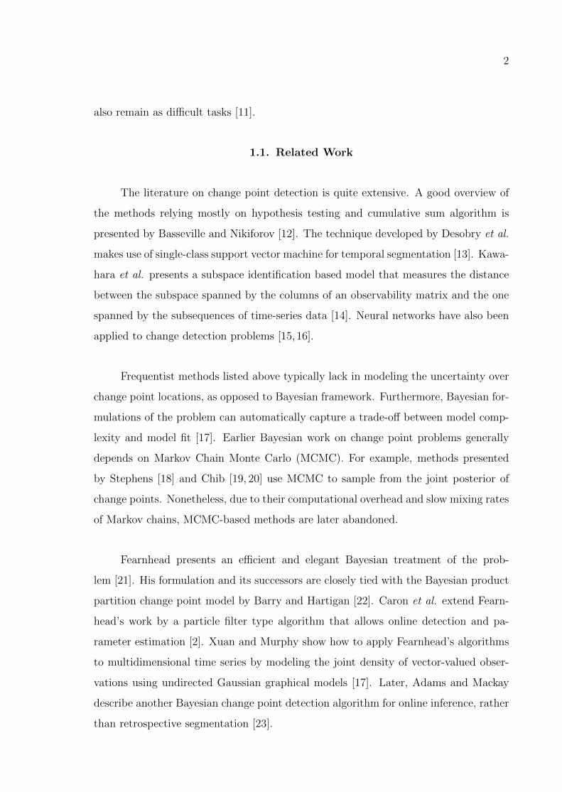
Change point detection techniques have proven useful in a diverse array of ap-

plications. In industrial contexts, such models have been used for quality control [3]

and measuring and controlling market risk [4]. Biology related applications include

but are not limited to the segmentation of electroencephalogram (EEG) signals [5, 6],

microarray data [7] and deoxyribonucleic acid (DNA) sequences [8]. Network intrusion

detection can also be noted as another application domain [9, 10].

Above-mentioned applications do not come as a free lunch. The problem inher-

ently incorporates certain issues that ought to be taken into consideration. First and

foremost, determining the number of change points as well as their locations simultane-

ously is a remarkable challenge. In case of multiple time series, one would presumably

like to take advantage of possibly correlated time series. Online detection of change

point locations and algorithms that are designed particularly for lengthy time series

2

also remain as difficult tasks [11].

1.1. Related Work

The literature on change point detection is quite extensive. A good overview of

the methods relying mostly on hypothesis testing and cumulative sum algorithm is

presented by Basseville and Nikiforov [12]. The technique developed by Desobry et al.

makes use of single-class support vector machine for temporal segmentation [13]. Kawa-

hara et al. presents a subspace identification based model that measures the distance

between the subspace spanned by the columns of an observability matrix and the one

spanned by the subsequences of time-series data [14]. Neural networks have also been

applied to change detection problems [15,16].

Frequentist methods listed above typically lack in modeling the uncertainty over

change point locations, as opposed to Bayesian framework. Furthermore, Bayesian for-

mulations of the problem can automatically capture a trade-off between model comp-

lexity and model fit [17]. Earlier Bayesian work on change point problems generally

depends on Markov Chain Monte Carlo (MCMC). For example, methods presented

by Stephens [18] and Chib [19, 20] use MCMC to sample from the joint posterior of

change points. Nonetheless, due to their computational overhead and slow mixing rates

of Markov chains, MCMC-based methods are later abandoned.

Fearnhead presents an efficient and elegant Bayesian treatment of the prob-

lem [21]. His formulation and its successors are closely tied with the Bayesian product

partition change point model by Barry and Hartigan [22]. Caron et al. extend Fearn-

head’s work by a particle filter type algorithm that allows online detection and pa-

rameter estimation [2]. Xuan and Murphy show how to apply Fearnhead’s algorithms

to multidimensional time series by modeling the joint density of vector-valued obser-

vations using undirected Gaussian graphical models [17]. Later, Adams and Mackay

describe another Bayesian change point detection algorithm for online inference, rather

than retrospective segmentation [23].

3

1.2. Scope of the Thesis

We approach the change point detection problem from a Bayesian standpoint.

More specifically, we describe a probabilistic graphical model and forward-backward

type recursion for exact inference on multivariate data. Inferred variables denote our

belief over change point locations as well as the latent dynamics within each segment.

The recursions are designed both for online and offline scenarios; thus, the model can

be applied to a large number of real-world problems.

In this thesis, we are concerned with the detection of Distributed Denial of Ser-

vice (DDoS) attacks in Session Initiation Protocol (SIP) networks. A DDoS attack

is defined as an explicit effort to overwhelm the processing power of a computer in

order to prevent the legitimate use of a service. The problem is ever-growing since

the attackers invent more sophisticated strategies as the Internet becomes more and

more complex. The classical way of performing a DDoS attack is flooding the target

computer by massive amounts of network packets [24]. Thus one would expect bursts

in the counts of packets arriving and leaving the network of the target computer under

a DDoS attack, which shows that our model is indeed plausible.

The main contributions of this thesis are the libraries that generate and collect

SIP network traffic data, the change point model, a generic implementation of the

model and a novel application. Details are as follows:

• Simulator: The module used for generating SIP traffic. It initiates real-time

SIP calls between a number of users, whose characteristics are governed by a

probabilistic generative model.

• Monitor: Feature collecting unit. Deployed on a SIP server, it extracts features

from the network and operating system of the server, delivers collected data to a

client computer in real time, and saves them in order to reproduce experiments.

• Bayesian Change Point Model (BCPM): We describe a generic generative mo-

del as well as exact and efficient inference and parameter learning algorithms.

In addition, we present four specific instances of this generic formulation and

4

implement the model as an open source C++ library [25].

• DDoS Attack Detection: We conduct extensive experiments on the synthetic data

generated by Simulator and a DDoS attack generating tool, and report the feature

sets and model parameters that yield the best performance.

1.3. Organization of the Thesis

The rest of the thesis is organized as follows: We first provide the necessary back-

ground information to remind the main concepts this thesis is built upon. The first

part of Chapter 3 explains our Bayesian change point model formulation, describes the

inference and parameter learning algorithms, and specifies the generative model. The

rest of this chapter is devoted to a detailed analysis of a particular model specifica-

tion: Dirichlet-Multinomial model. Chapter 4 covers our SIP network data generation

mechanism, experiment setup and the results. Finally, Chapter 5 concludes this thesis.

5

2. THEORETICAL BACKGROUND

This chapter is devoted to provide the theoretical background needed to under-

stand subsequent parts of the thesis. We first examine different time series models

in general terms and introduce our notation. Following section covers Expectation-

Maximization (EM) algorithm for parameter estimation in latent state models. We

finally give a brief overview of Nonnegative Matrix Factorization (NMF).

2.1. Time Series Models

The simplest way to model a data set is to assume that the instances are in-

dependent and identically distributed (iid) random variables. In applications such as

speech recognition, stock market prediction, DNA sequence analysis, etc, however,

this assumption would not properly model sequential dependencies. Therefore, iid as-

sumption must be relaxed in problems that involve temporal relations. Probabilistic

graphical models are powerful tools to model such dependencies as well as the uncer-

tainty in the data. For time series data v1, v2, . . . , vt, a graphical model specifies the

joint distribution p(v1, v2, . . . , vt). Our standard notation for such sequential data is

given below:

v1:T ≡ v1, v2, . . . , vt (2.1)

2.1.1. Markov Model

When we assume that the observation at time t depends only on the most re-

cent observation, we obtain a first-order Markov chain. Mathematically, underlying

modeling assumption is the following:

p(vt|v1, v2, . . . , vt−1) = p(vt|vt−1) (2.2)

6

The joint distribution over all variables can then be factorized as follows:

p(v1:T ) = p(v1)T∏t=2

p(vt|vt−1) (2.3)

Although a first-order Markov chain is conceptually sound and easy to implement,

it lacks in anticipating patterns involving several consecutive data instances. One way

to extend the model is to consider Markov chains of higher orders. More concretely,

we may form an L’th order Markov chain if we allow the variable at time t to depend

on previous L observations:

p(vt|v1, v2, . . . , vt−1) = p(vt|vt−L, . . . , vt−1) (2.4)

Graphical models associated with the first-order and second-order Markov models are

depicted in Figure 2.1.

When the observations are discrete and can take at most N values, a first-order

Markov model can be parameterized by an N ×N transition matrix. Similarly, transi-

tion probabilities of an L’th order Markov chain are specified by a K + 1 dimensional

array, which implies that the number of parameters required grows exponentially with

the order of the chain.

2.1.2. Hidden Markov Model

In hidden Markov models (HMMs), we assume that each observation is a prob-

abilistic function of a latent (hidden) state. Furthermore, in contrast to observable

Markov model, a Markov chain is formed on latent states, not the observations. Con-

sequently, this setup provides a more general framework for time series analysis and

does not require exponentially many parameters - as long as the chain is of order one.

Graphical model of a hidden Markov model is given in Figure 2.2. Note that shaded

nodes in all graphical models in this thesis represent observations whereas the remain-

7

v1 v2 v3 v4 ... vt ...

v1 v2 v3 v4 ... vt ...

Figure 2.1. Graphical models of first-order and second-order Markov models

ing nodes are hidden variables.

Joint distribution corresponding to the model in Figure 2.2 is given by

p(h1:T , v1:T ) = p(h1)

[T∏t=2

p(ht|ht−1)

][T∏t=1

p(vt|ht)

](2.5)

The hidden variable ht in an HMM is always discrete whereas the observation

model can either be discrete or continuous. When ht can take N different values, we

use an N × N matrix A to denote the state transition probabilities. More explicitly,

Aij = p(ht = i|ht−1 = j) denotes the probability of going from state j to state i at any

time t. In this notation, A is a column stochastic matrix,∑

iAij = 1, and made up

of nonnegative entries, Aij ≥ 0. In case of discrete observations, vt ∈ 1, 2, . . . ,M,

another column stochastic matrix C represents observation (emission) probabilities:

Cij = p(vt = i|ht = j) is the probability of observing i, being in state j. We again have∑iCij = 1 and Cij ≥ 0.

h1 h2 h3... ht

...

v1 v2 v3 ... vt ...

Figure 2.2. Graphical model of hidden Markov model

8

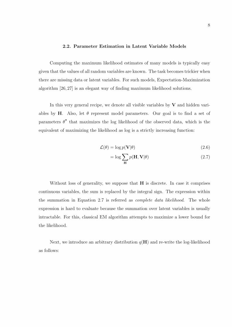
2.2. Parameter Estimation in Latent Variable Models

Computing the maximum likelihood estimates of many models is typically easy

given that the values of all random variables are known. The task becomes trickier when

there are missing data or latent variables. For such models, Expectation-Maximization

algorithm [26,27] is an elegant way of finding maximum likelihood solutions.

In this very general recipe, we denote all visible variables by V and hidden vari-

ables by H. Also, let θ represent model parameters. Our goal is to find a set of

parameters θ* that maximizes the log likelihood of the observed data, which is the

equivalent of maximizing the likelihood as log is a strictly increasing function:

L(θ) = log p(V|θ) (2.6)

= log∑H

p(H,V|θ) (2.7)

Without loss of generality, we suppose that H is discrete. In case it comprises

continuous variables, the sum is replaced by the integral sign. The expression within

the summation in Equation 2.7 is referred as complete data likelihood. The whole

expression is hard to evaluate because the summation over latent variables is usually

intractable. For this, classical EM algorithm attempts to maximize a lower bound for

the likelihood.

Next, we introduce an arbitrary distribution q(H) and re-write the log-likelihood

as follows:

9

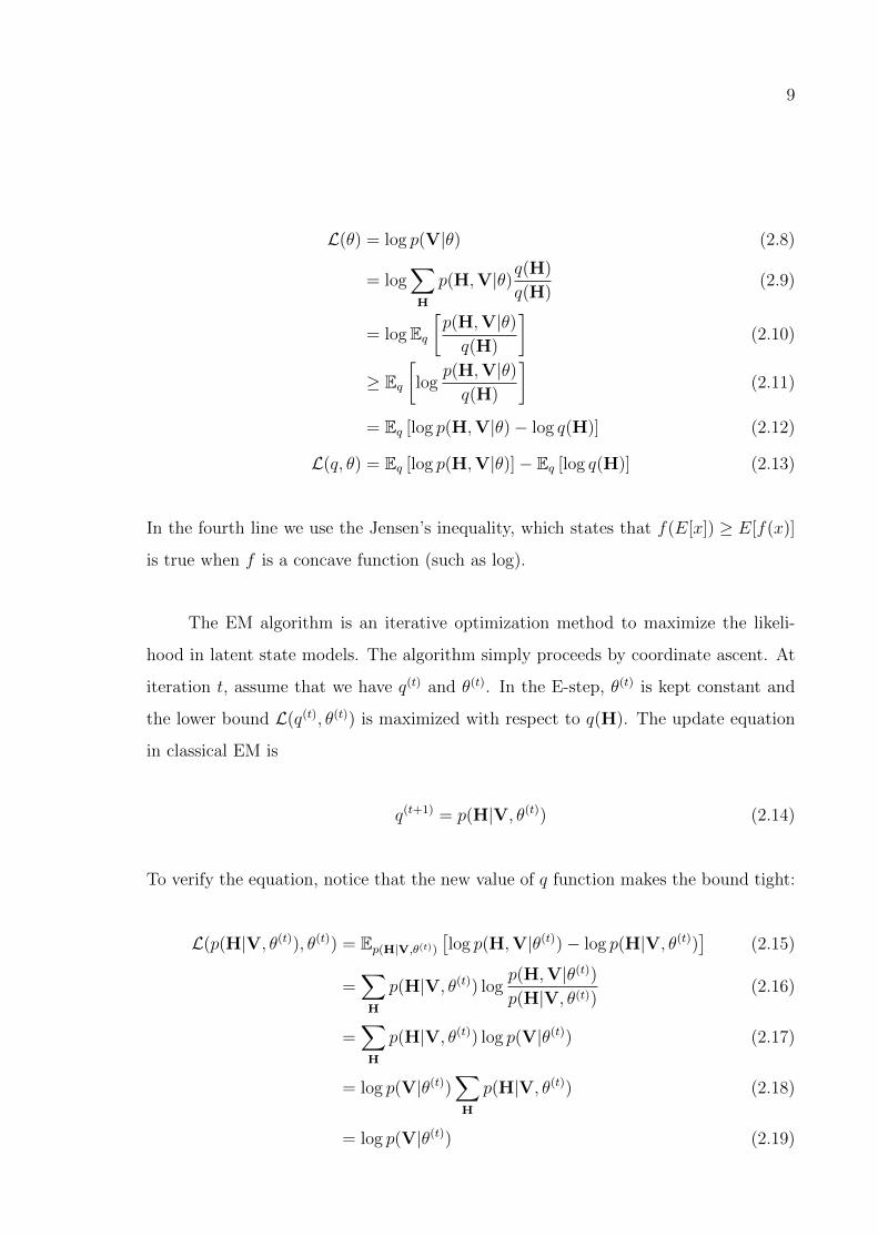
L(θ) = log p(V|θ) (2.8)

= log∑H

p(H,V|θ)q(H)

q(H)(2.9)

= logEq[p(H,V|θ)q(H)

](2.10)

≥ Eq[log

p(H,V|θ)q(H)

](2.11)

= Eq [log p(H,V|θ)− log q(H)] (2.12)

L(q, θ) = Eq [log p(H,V|θ)]− Eq [log q(H)] (2.13)

In the fourth line we use the Jensen’s inequality, which states that f(E[x]) ≥ E[f(x)]

is true when f is a concave function (such as log).

The EM algorithm is an iterative optimization method to maximize the likeli-

hood in latent state models. The algorithm simply proceeds by coordinate ascent. At

iteration t, assume that we have q(t) and θ(t). In the E-step, θ(t) is kept constant and

the lower bound L(q(t), θ(t)) is maximized with respect to q(H). The update equation

in classical EM is

q(t+1) = p(H|V, θ(t)) (2.14)

To verify the equation, notice that the new value of q function makes the bound tight:

L(p(H|V, θ(t)), θ(t)) = Ep(H|V,θ(t))[log p(H,V|θ(t))− log p(H|V, θ(t))

](2.15)

=∑H

p(H|V, θ(t)) logp(H,V|θ(t))p(H|V, θ(t))

(2.16)

=∑H

p(H|V, θ(t)) log p(V|θ(t)) (2.17)

= log p(V|θ(t))∑H

p(H|V, θ(t)) (2.18)

= log p(V|θ(t)) (2.19)

10

The M-Step updates the model parameter θ(t) to maximize L(q, θ) while holding

the distribution q(t+1) unchanged. Observe that the second term on the right hand

side of the equality in Equation 2.13 is constant with respect to θ. Thus, this step

only maximizes Eq[log p(H,V|θ(t))

], which is referred as expected complete data log

likelihood. The update equation is the following:

θ(t+1) = argmaxθ(t)

L(q(t+1), θ(t)) (2.20)

A nice property of the algorithm is that neither step causes a decrease in the log

likelihood. In order to show that, we first need to define the Kullback-Leibler (KL)

divergence [28]. KL divergence is a distance measure between two distributions p(x)

and q(x), and is defined as follows:

KL(p||q) = −∫p(x) log

q(x)

p(x)dx (2.21)

KL divergence is always non-negative, KL(p||q) ≥ 0, and equality holds if and only if

p(x) = q(x). Also, it is not symmetrical quantity: KL(p||q) 6= KL(q||p).

Now, let us re-write the log likelihood:

L(θ) = log p(V|θ) (2.22)

=∑H

log p(H,V|θ)− log p(H|V, θ) (2.23)

=∑H

q(H) (log p(H,V|θ)− log p(H|V, θ) + log q(H)− log q(H)) (2.24)

=∑H

q(H)

(log

p(H,V|θ)q(H)

− logp(H|V, θ)q(H)

)(2.25)

=∑H

q(H)

(log

p(H,V|θ)q(H)

)−∑H

q(H)

(log

p(H|V, θ)q(H)

)(2.26)

= L(q, θ) + KL(q||p) (2.27)

11

In E-step, q distribution is set to the posterior distribution p(H|V, θ(t)). There-

fore, KL-divergence in Equation 2.27 vanishes, and the lower bound is equal to the

log likelihood. Because E-step maximizes the lower bound, L(θ) increases or stays the

same if the maximum is already attained. In M-step, the model parameters are set to

maximize the lower bound L(q, θ). Furthermore, q distribution, which is held constant

in this step, was computed conditioned on the old parameters. Hence, it must be dif-

ferent than the new posterior distribution p(H|V, θ(t+1)): KL(q||p) > 0. Overall, log

likelihood, L(θ) increases. The algorithm terminates when it converges to some value.

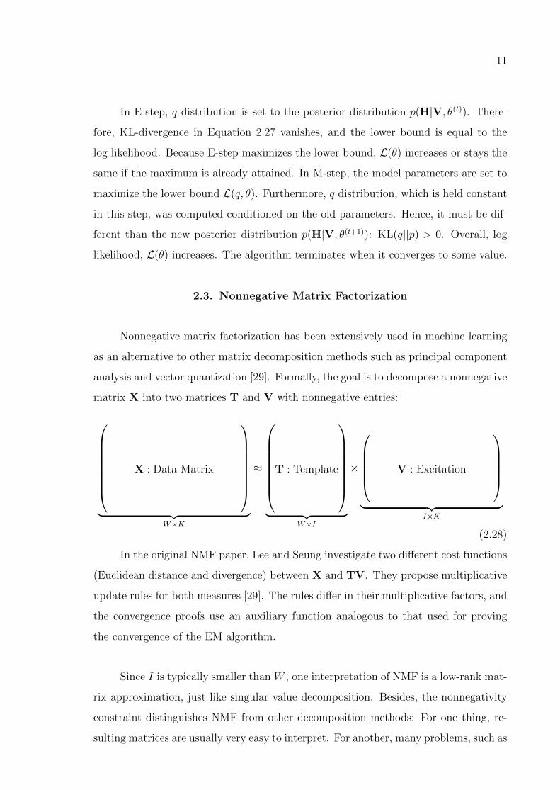
2.3. Nonnegative Matrix Factorization

Nonnegative matrix factorization has been extensively used in machine learning

as an alternative to other matrix decomposition methods such as principal component

analysis and vector quantization [29]. Formally, the goal is to decompose a nonnegative

matrix X into two matrices T and V with nonnegative entries:

X : Data Matrix

︸︷︷︸

W×K

≈

T : Template

︸︷︷︸

W×I

×

V : Excitation

︸︷︷︸

I×K

(2.28)

In the original NMF paper, Lee and Seung investigate two different cost functions

(Euclidean distance and divergence) between X and TV. They propose multiplicative

update rules for both measures [29]. The rules differ in their multiplicative factors, and

the convergence proofs use an auxiliary function analogous to that used for proving

the convergence of the EM algorithm.

Since I is typically smaller than W , one interpretation of NMF is a low-rank mat-

rix approximation, just like singular value decomposition. Besides, the nonnegativity

constraint distinguishes NMF from other decomposition methods: For one thing, re-

sulting matrices are usually very easy to interpret. For another, many problems, such as

12

source separation and image processing, by nature require T and V to be nonnegative.

Therefore, NMF has received a lot of attention in recent years.

The update equations presented in [29] provide point estimates for the template

and excitation matrices. Consequently, the matrices may easily overfit the data and

certainly lack in modeling uncertainty. Cemgil approaches NMF from a Bayesian stand-

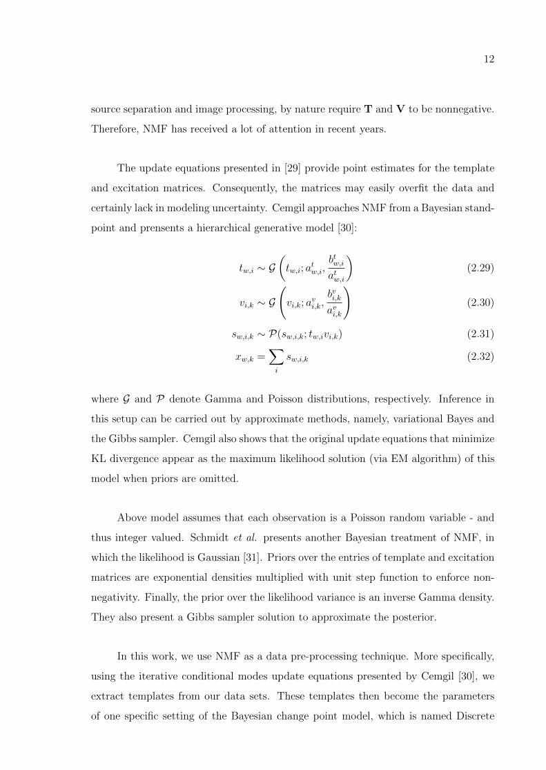
point and prensents a hierarchical generative model [30]:

tw,i ∼ G(tw,i; a

tw,i,

btw,iatw,i

)(2.29)

vi,k ∼ G

(vi,k; a

vi,k,

bvi,kavi,k

)(2.30)

sw,i,k ∼ P(sw,i,k; tw,ivi,k) (2.31)

xw,k =∑i

sw,i,k (2.32)

where G and P denote Gamma and Poisson distributions, respectively. Inference in

this setup can be carried out by approximate methods, namely, variational Bayes and

the Gibbs sampler. Cemgil also shows that the original update equations that minimize

KL divergence appear as the maximum likelihood solution (via EM algorithm) of this

model when priors are omitted.

Above model assumes that each observation is a Poisson random variable - and

thus integer valued. Schmidt et al. presents another Bayesian treatment of NMF, in

which the likelihood is Gaussian [31]. Priors over the entries of template and excitation

matrices are exponential densities multiplied with unit step function to enforce non-

negativity. Finally, the prior over the likelihood variance is an inverse Gamma density.

They also present a Gibbs sampler solution to approximate the posterior.

In this work, we use NMF as a data pre-processing technique. More specifically,

using the iterative conditional modes update equations presented by Cemgil [30], we

extract templates from our data sets. These templates then become the parameters

of one specific setting of the Bayesian change point model, which is named Discrete

13

model and detailed in Subsection 3.1.5.4. Also, Figures 4.3 and 4.4 depict the template

and excitation matrices inferred by the algorithm when executed on the network traffic

data.

14

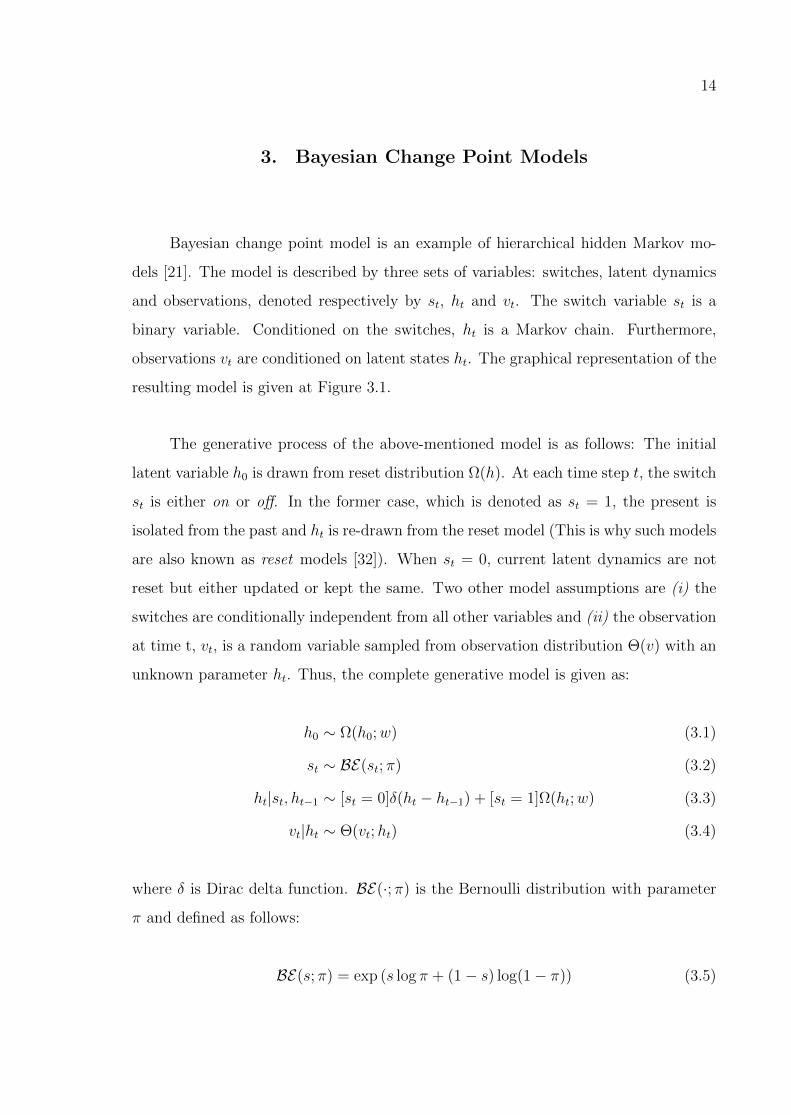
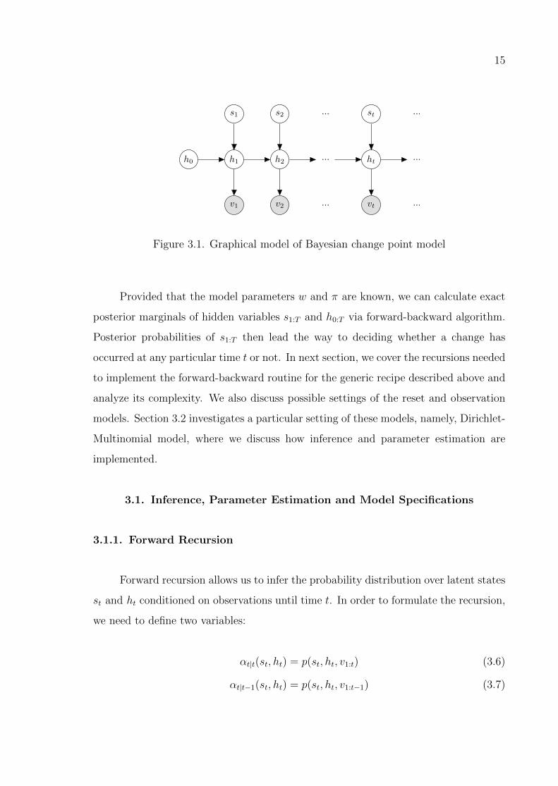
3. Bayesian Change Point Models

Bayesian change point model is an example of hierarchical hidden Markov mo-

dels [21]. The model is described by three sets of variables: switches, latent dynamics

and observations, denoted respectively by st, ht and vt. The switch variable st is a

binary variable. Conditioned on the switches, ht is a Markov chain. Furthermore,

observations vt are conditioned on latent states ht. The graphical representation of the

resulting model is given at Figure 3.1.

The generative process of the above-mentioned model is as follows: The initial

latent variable h0 is drawn from reset distribution Ω(h). At each time step t, the switch

st is either on or off. In the former case, which is denoted as st = 1, the present is

isolated from the past and ht is re-drawn from the reset model (This is why such models

are also known as reset models [32]). When st = 0, current latent dynamics are not

reset but either updated or kept the same. Two other model assumptions are (i) the

switches are conditionally independent from all other variables and (ii) the observation

at time t, vt, is a random variable sampled from observation distribution Θ(v) with an

unknown parameter ht. Thus, the complete generative model is given as:

h0 ∼ Ω(h0;w) (3.1)

st ∼ BE(st; π) (3.2)

ht|st, ht−1 ∼ [st = 0]δ(ht − ht−1) + [st = 1]Ω(ht;w) (3.3)

vt|ht ∼ Θ(vt;ht) (3.4)

where δ is Dirac delta function. BE(·; π) is the Bernoulli distribution with parameter

π and defined as follows:

BE(s; π) = exp (s log π + (1− s) log(1− π)) (3.5)

15

h0 h1 h2... ht

...

s1 s2 ... st ...

v1 v2 ... vt ...

Figure 3.1. Graphical model of Bayesian change point model

Provided that the model parameters w and π are known, we can calculate exact

posterior marginals of hidden variables s1:T and h0:T via forward-backward algorithm.

Posterior probabilities of s1:T then lead the way to deciding whether a change has

occurred at any particular time t or not. In next section, we cover the recursions needed

to implement the forward-backward routine for the generic recipe described above and

analyze its complexity. We also discuss possible settings of the reset and observation

models. Section 3.2 investigates a particular setting of these models, namely, Dirichlet-

Multinomial model, where we discuss how inference and parameter estimation are

implemented.

3.1. Inference, Parameter Estimation and Model Specifications

3.1.1. Forward Recursion

Forward recursion allows us to infer the probability distribution over latent states

st and ht conditioned on observations until time t. In order to formulate the recursion,

we need to define two variables:

αt|t(st, ht) = p(st, ht, v1:t) (3.6)

αt|t−1(st, ht) = p(st, ht, v1:t−1) (3.7)

16

These are refered as forward and forward-predict variables, respectively. What is

called filtered change point probability p(st|v1:t) can then be expressed as a function of

the forward message:

p(st|v1:t) =

∫p(st, ht|v1:t)dht (3.8)

∝∫αt|t(st, ht)dht (3.9)

As new observations arrive, forward-predict and forward messages are alternatively

calculated and the posterior probabilities of latent states are propagated as follows:

αt|t(st, ht) = p(st, ht, v1:t) (3.10)

= p(vt|st, ht) p(st, ht, v1:t−1)︸︷︷︸αt|t−1(st−1,ht−1)

(3.11)

= p(vt|ht)∑st−1

∫p(st−1, ht−1, st, ht, v1:t−1)dht−1 (3.12)

= p(vt|ht)∑st−1

∫p(st−1, ht−1, v1:t−1)p(st, ht|st−1, ht−1)dht−1 (3.13)

= p(vt|ht)∑st−1

∫αt−1|t−1(st−1, ht−1)p(ht|st, ht−1)p(st)dht−1 (3.14)

= p(vt|ht)∑st−1

∫αt−1|t−1(st−1, ht−1)

(δ(ht − ht−1)p(st = 0)+

p(ht)p(st = 1))dht−1 (3.15)

3.1.2. Backward Recursion

Similar to forward messages, backward messages (beta-postdict and beta, respec-

tively) are defined as follows:

βt−1|t(st−1, ht−1) = p(vt:T |st−1, ht−1) (3.16)

βt|t(st, ht) = p(vt:T |st, ht) (3.17)

17

Product of beta-postdict message and the observation model gives the beta message

as shown below:

βt|t(st, ht) = βt|t+1(st, ht)p(vt|ht) (3.18)

We now examine the backward propagation step:

βt−1|t(st−1, ht−1) = p(vt:T |st−1, ht−1) (3.19)

=∑st

∫p(vt:T , st, ht|st−1, ht−1)dht (3.20)

=∑st

∫p(vt:T |st, ht)p(st, ht|st−1, ht−1)dht (3.21)

=∑st

∫βt|t(st, ht)p(ht|st, ht−1)p(st)dht (3.22)

=

∫βt|t(st, ht)

(δ(ht − ht−1)p(st = 0) + p(ht)p(st = 1)

)dht (3.23)

3.1.3. Smoothing

Posterior probabilities conditioned on full history can be obtained by multiplying

forward and backward messages:

p(st, ht|v1:T ) ∝ p(st, ht, v1:T ) (3.24)

= p(st, ht, v1:t)p(vt+1:T |st, ht, v1:t) (3.25)

= p(st, ht, v1:t)p(vt+1:T |st, ht) (3.26)

= αt|t(st, ht)βt|t+1(st, ht) (3.27)

When the inference task is online, using forward filtered change point probabilities

is appropriate. In cases where a small amount of delay in change point decision at time

t is allowed, one may use evidence from future in addition to the observations up to

time t. For such cases, we use online (fixed lag) smoothers, in which a fixed number of

18

backward recursions are performed after each new observation. This fixed number is

known as lag. If the lag is L, posterior probabilities at time t are calculated conditioned

on the observations up to time t+ L, as formulated below:

p(st, ht, v1:t+L) = p(st, ht, v1:t)p(vt+1:t+L|st, ht) (3.28)

The second expression on the right hand side of the equality is computed by executing

backward recursions for L steps, starting from the observation at time t+ L.

3.1.4. Parameter Estimation

At the beginning of the inference, we assumed that model parameters are known

beforehand. Simple search techniques for setting parameters to appropriate values,

like grid search, may work in practice but are not typically scalable to large problems.

The EM algorithm is a well-known tool in statistical estimation problems involving

incomplete data. In this subsection, we derive an EM algorithm to estimate model pa-

rameters that maximize the (log)likelihood. Formally, our goal is to estimate θ = (w, π)

that maximize

L(θ) = log p(s1:T , h0:T , v1:T , |θ) (3.29)

= log Ω(h0;w) +T∑t=1

[[st = 0]

(log(1− π) + log δ(ht − ht−1)

)+ [st = 1]

(log π + log Ω(ht;w)

)+ log Θ(vt;ht)

](3.30)

3.1.4.1. E-Step. The EM recipe presented in Section 2.2 requires us to take the ex-

pectation of Equation 3.30 with respect to the posterior distribution. If we denote the

posterior at τ ’th step of the algorithm as p(s1:T , h0:T |v1:T , θ(τ)), the expectation of L(θ)

19

with respect to the posterior is given by the following:

Ep(s1:T ,h0:T |v1:T ,θ(τ))[L(θ)] =T∑t=1

Ep(s1:T ,h0:T |v1:T ,θ(τ))[[st = 0]

(log(1− π)

)]+

T∑t=1

Ep(s1:T ,h0:T |v1:T ,θ(τ))[[st = 1]

(log π + log Ω(ht;w)

)]+ Ep(s1:T ,h0:T |v1:T ,θ(τ))[log Ω(h0;w)]

+T∑t=1

Ep(s1:T ,h0:T |v1:T ,θ(τ))[

log Θ(vt;ht)]

(3.31)

= log(1− π)T∑t=1

p(st = 0|v1:T , θ(τ))

+ log πT∑t=1

p(st = 1|v1:T , θ(τ))

+T∑t=0

p(st = 1|v1:T , θ(τ))Ep(ht|v1:T ,θ(τ))[

log Ω(ht;w)]

+T∑t=1

Ep(ht|v1:T ,θ(τ))[

log Θ(vt;ht)]

(3.32)

where we introduce an auxillary variable s0 and set p(s0 = 1|v1:T , θ(τ)) = 1 for com-

pactness in the notation.

3.1.4.2. M-Step. In this step, we maximize Equation 3.32 with respect to w and π

by taking partial derivatives. Observe that the last summation in Equation 3.32 is

independent of the parameters and thus can be omitted. Partial derivative with respect

to π yields:

0 =∂Ep(s1:T ,h0:T |v1:T ,θ(τ))[L(θ)]

∂π(3.33)

=1

π

T∑t=1

p(st = 1|v1:T , θ(τ))−1

1− π

T∑t=1

p(st = 0|v1:T , θ(τ)) (3.34)

π(τ+1) =1

T

T∑t=1

p(st = 1|v1:T , θ(τ)) (3.35)

20

Above equation tells us to set the new value of the prior to the average of posterior

change point probabilities, which we find very intiutive. Maximization with respect to

w involves a single term:

0 =∂Ep(s1:T ,h0:T |v1:T ,θ(τ))[L(θ)]

∂w(3.36)

=T∑t=0

p(st = 1|v1:T , θ(τ))∂

∂wEp(ht|v1:T ,θ(τ))

[log Ω(ht;w)

](3.37)

The term in Equation 3.37 depends directly on the Ω distribution. Once the derivative

is computed for different reset models, a general framework incorparating the algorithm

is straightforward to implement.

3.1.5. Model Specifications

Inference and parameter learning methods presented so far are independent of

the observation model Θ and reset model Ω. Depending on the application and data

set characteristics, these models can be set appropriately. A significant point is that

the computations are much easier if the models are discrete or Θ is the conjugate prior

of Ω since the inference requires their product. Below are four reset/observation model

pairs we investigate in this thesis:

3.1.5.1. Gamma-Poisson (GP) Model. Given a data set consisting of nonnegative in-

tegers, this model assumes that the observation vt is a Poisson random variable with

intensity parameter ht [21,33]. Gamma distribution is an appropriate choice to model

the uncertainty over unknown Poisson intensity since both its support and intensity

parameters are positive real numbers. Consequently, reset hyperparameter is a couple

of real numbers, w = (a, b), which denote the shape and scale parameters of Gamma

distribution. As a consequence, forward and backward messages in this setup store

a mixture of Gamma potentials over ht. Below are the probability distribution/mass

21

functions of Gamma and Poisson distributions:

Ω(h;w) = G(h; a, b) =ba

Γ(a)ha−1e−bh (3.38)

Θ(v;h) = P(v;h) =hve−h

Γ(v + 1)(3.39)

When the problem is multidimensional, one may treat each feature as an independent

Poisson random variable. In this case, the intensity parameters are either reset alto-

gether or stay the same. Obviously, the model defined by Equations 3.38 and 3.39 is

one-dimensional instance of this more general formulation.

3.1.5.2. Dirichlet-Multinomial (DM) Model. If the observations are K ≥ 2 dimen-

sional vectors of nonnegative integers, they could be treated as Multinomial random

variables. This assumption enforces the latent variable ht to be a K ≥ 2 dimensional

vector whose elements are nonnegative and sum up to 1. Dirichlet distribution fits this

setup very well since it is a distribution over K−simplex, which includes any possible

value of ht:

Ω(h; w) = Dir(h; w) =Γ(∑K

k=1wk

)∏K

k=1 Γ(wk)

K∏k=1

hwk−1k (3.40)

Θ(v; h) =M(v; h) =Γ(∑

k vk + 1)∏k Γ(vk + 1)

∏k

hvkk (3.41)

where Dir andM stand for Dirichlet and Multinomial distributions, respectively. One

may similarly build a Dirichlet-Categorical model if the observations are vectors with

one element being 1 and other elements being 0.

3.1.5.3. Compound Model. It is also possible to consider a compound model, in which

a pre-determined subset of features is modeled with DM model and GP model is used

for the rest. Without loss of generality, we may assume that the features can be

arranged in such a way that the first M entries of an N dimensional observation vector

v form the first subset and the last N −M entries form the second one. We denote the

22

resulting hyperparameter as w = α1:M , a1:N−M , b1:N−M and the Compound model is

defined as follows:

Ω(h; w) = Dir(h1:M ;α1:M)×N−M∏i=1

G(hi+M ; ai, bi) (3.42)

Θ(v; h) =M(v1:M ;h1:M)×N−M∏i=1

P(vi+M ;hi+M) (3.43)

One may notice that even if we omit the DM part, i.e., M = 0, Equations 3.42 and 3.43

still define a compound (GP) model, provided N > 1. Also, the generative model of

our BCPM enforces a binary change decision, that is to say, the latent parameters are

reset altogether in case of a change.

3.1.5.4. Discrete Model. A discrete BCPM assumes that the system being examined

can be at 1 of K possible states. As opposed to DM/GP models, a latent state ht in this

setup does not track the parameter of the observation model but the probability mass

over all states. Hence, ht is modeled as a categorical random variable. We furthermore

assume that the observations are Multinomial and that each state k is associated with

its own emission probability vector tk. The overall model is expressed below:

Ω(h; w) = Cat(h,w) =K∏k=1

w[h=k]k (3.44)

Θ(v;h, t1:K) =K∏k=1

M(v; tk)[h=k] (3.45)

where Cat denotes Categorical distribution.

3.1.6. Complexity Analysis of Forward-Backward

When the state space of ht is discrete as in Subsection 3.1.5.4, the model reduces

to classical HMMs, where the latent state space is simply the Cartesian product of that

of st and ht. In this case, forward variables are 2 × |ht| dimensional matrices, where

|ht| denotes the length of the hidden variable. Nonetheless, other model specifications

23

are in continuous domain and require more detailed analysis.

As we try to sum over exponentially many possible switch settings to calculate the

posterior, the inference might seem intractable at first glance. However, thanks to the

forgetting (reset) property of the model, it is possible to implement forward-backward

routine efficiently, i.e., quadratic with the number of observations T . We first define

the two components of the forward message given in Equation 3.15 as follows:

p(st = 0, ht, v1:t) = p(vt|ht)∑st−1

∫p(st−1, ht−1, v1:t−1)δ(ht − ht−1)p(st = 0)dht−1

= p(vt|ht)p(ht, v1:t−1)p(st = 0) (3.46)

p(st = 1, ht, v1:t) = p(vt|ht)∑st−1

∫p(st−1, ht−1, v1:t−1)p(ht)p(st = 1)dht−1

= p(vt|ht)p(v1:t−1)p(ht)p(st = 1) (3.47)

In our terminology, components in Equations 3.46 and 3.47 denote no-change

and change cases. In a no-change case, the forward message at time t− 1 is multiplied

by observation probability and change point prior. Informally speaking, probability

distribution over ht−1 is updated and transferred to ht, due to the integral and Dirac

delta function. In a change case however, p(ht) is reset to Ω(ht;w), meaning it becomes

a single component whose parameter is independent of previous message.

Overall, the forward message αt|t(st, ht) is computed by updating the previous

message (formulated in no-change case) and adding one more component (change case).

Therefore, in general, if αt−1|t−1(st−1, ht−1) is a mixture with K components, the next

forward message would have K + 1 components. In other words, the number of com-

ponents grows only linearly with time, and filtering consequently scales with O(T 2).

For smoothing, we multiply forward and backward messages; hence, the complexity

becomes O(T 4). Similarly, executing fixed lag smoothing, with lag being L, requires

O(T 2L) computational load.

24

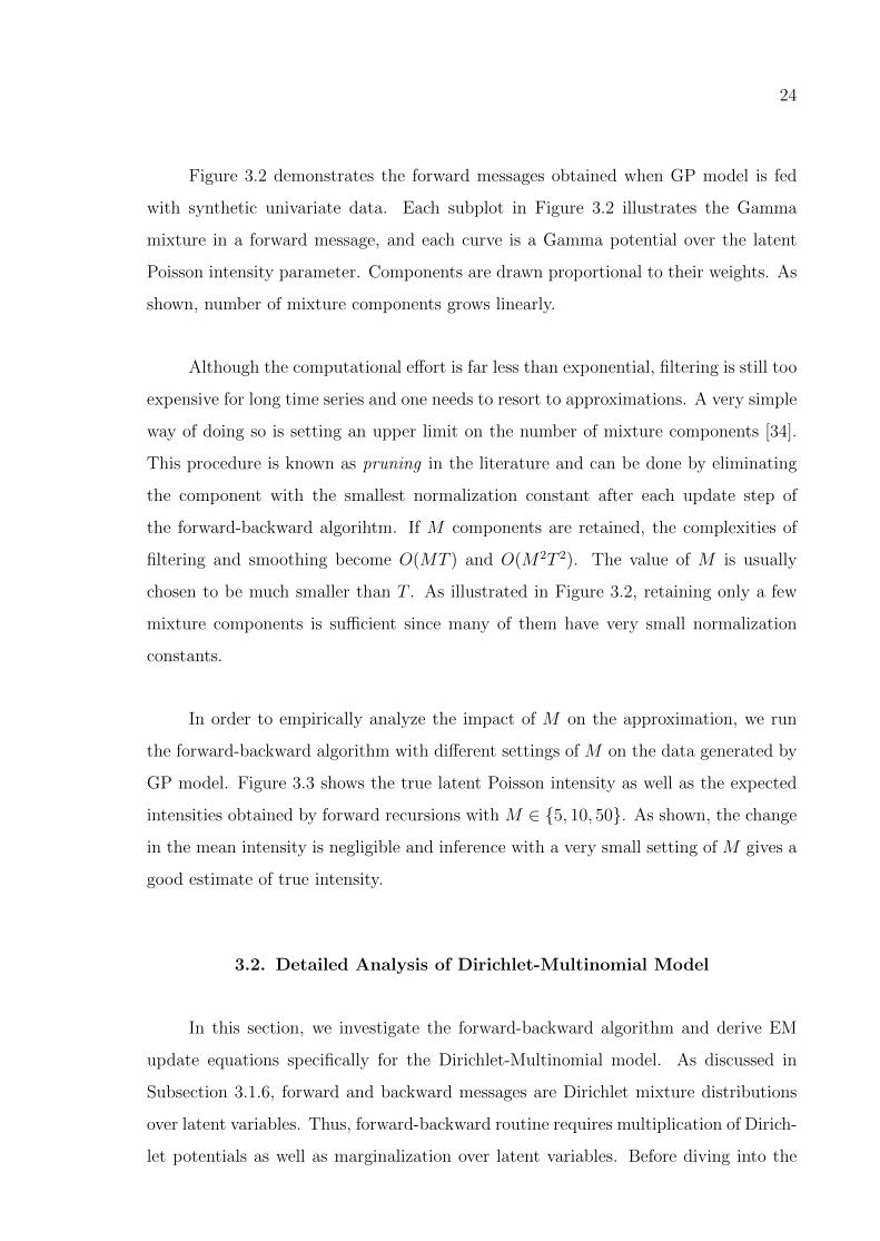
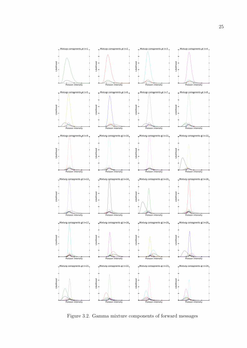
Figure 3.2 demonstrates the forward messages obtained when GP model is fed

with synthetic univariate data. Each subplot in Figure 3.2 illustrates the Gamma

mixture in a forward message, and each curve is a Gamma potential over the latent

Poisson intensity parameter. Components are drawn proportional to their weights. As

shown, number of mixture components grows linearly.

Although the computational effort is far less than exponential, filtering is still too

expensive for long time series and one needs to resort to approximations. A very simple

way of doing so is setting an upper limit on the number of mixture components [34].

This procedure is known as pruning in the literature and can be done by eliminating

the component with the smallest normalization constant after each update step of

the forward-backward algorihtm. If M components are retained, the complexities of

filtering and smoothing become O(MT ) and O(M2T 2). The value of M is usually

chosen to be much smaller than T . As illustrated in Figure 3.2, retaining only a few

mixture components is sufficient since many of them have very small normalization

constants.

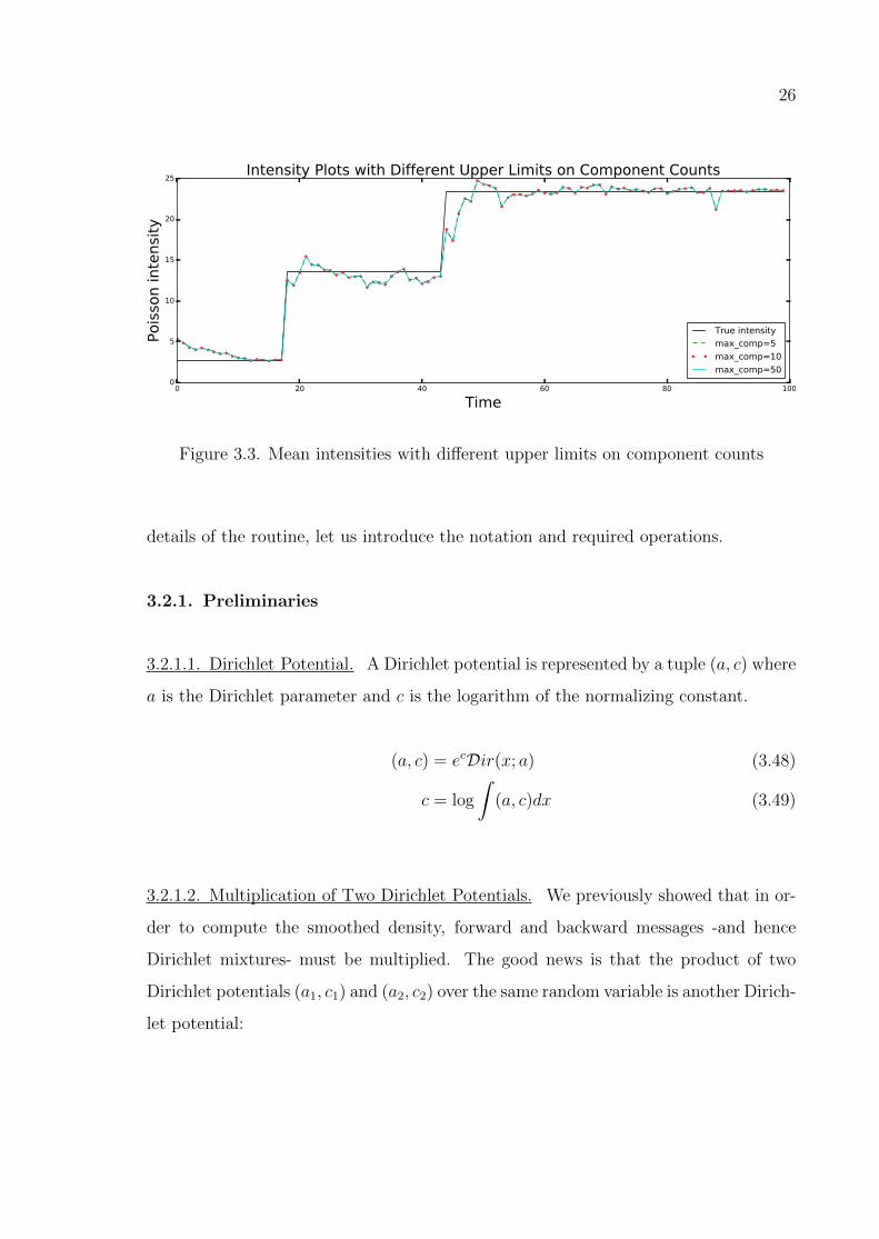
In order to empirically analyze the impact of M on the approximation, we run

the forward-backward algorithm with different settings of M on the data generated by

GP model. Figure 3.3 shows the true latent Poisson intensity as well as the expected

intensities obtained by forward recursions with M ∈ 5, 10, 50. As shown, the change

in the mean intensity is negligible and inference with a very small setting of M gives a

good estimate of true intensity.

3.2. Detailed Analysis of Dirichlet-Multinomial Model

In this section, we investigate the forward-backward algorithm and derive EM

update equations specifically for the Dirichlet-Multinomial model. As discussed in

Subsection 3.1.6, forward and backward messages are Dirichlet mixture distributions

over latent variables. Thus, forward-backward routine requires multiplication of Dirich-

let potentials as well as marginalization over latent variables. Before diving into the

25

0 5 10 15 20

Poisson intensity0.00

0.05

0.10

0.15

0.20

0.25

Like

lihood

Mixture components at t=1

0 5 10 15 20


0.05

0.10

0.15

0.20

0.25

Like

lihood


0 5 10 15 20


0.05

0.10

0.15

0.20

0.25

Like

lihood


0 5 10 15 20


0.05

0.10

0.15

0.20

0.25

Like

lihood


0 5 10 15 20


0.05

0.10

0.15

0.20

0.25

Like

lihood


0 5 10 15 20


0.05

0.10

0.15

0.20

0.25

Like

lihood


0 5 10 15 20


0.05

0.10

0.15

0.20

0.25

Like

lihood


0 5 10 15 20


0.05

0.10

0.15

0.20

0.25

Like

lihood


0 5 10 15 20


0.05

0.10

0.15

0.20

0.25

Like

lihood


0 5 10 15 20


0.05

0.10

0.15

0.20

0.25

Like

lihood


0 5 10 15 20


0.05

0.10

0.15

0.20

0.25Like

lihood


0 5 10 15 20


0.05

0.10

0.15

0.20

0.25

Like

lihood


0 5 10 15 20


0.05

0.10

0.15

0.20

0.25

Like

lihood


0 5 10 15 20


0.05

0.10

0.15

0.20

0.25

Like

lihood


0 5 10 15 20


0.05

0.10

0.15

0.20

0.25

Like

lihood


0 5 10 15 20


0.05

0.10

0.15

0.20

0.25

Like

lihood


0 5 10 15 20


0.05

0.10

0.15

0.20

0.25

Like

lihood


0 5 10 15 20


0.05

0.10

0.15

0.20

0.25

Like

lihood


0 5 10 15 20


0.05

0.10

0.15

0.20

0.25

Like

lihood


0 5 10 15 20


0.05

0.10

0.15

0.20

0.25

Like

lihood


0 5 10 15 20


0.05

0.10

0.15

0.20

0.25

Like

lihood


0 5 10 15 20


0.05

0.10

0.15

0.20

0.25

Like

lihood


0 5 10 15 20


0.05

0.10

0.15

0.20

0.25

Like

lihood


0 5 10 15 20


0.05

0.10

0.15

0.20

0.25

Like

lihood


Figure 3.2. Gamma mixture components of forward messages

26

0 20 40 60 80 100

Time

0

5

10

15

20

25

Poisson intensity

Intensity Plots with Different Upper Limits on Component Counts

True intensity

max_comp=5

max_comp=10

max_comp=50

Figure 3.3. Mean intensities with different upper limits on component counts

details of the routine, let us introduce the notation and required operations.

3.2.1. Preliminaries

3.2.1.1. Dirichlet Potential. A Dirichlet potential is represented by a tuple (a, c) where

a is the Dirichlet parameter and c is the logarithm of the normalizing constant.

(a, c) = ecDir(x; a) (3.48)

c = log

∫(a, c)dx (3.49)

3.2.1.2. Multiplication of Two Dirichlet Potentials. We previously showed that in or-

der to compute the smoothed density, forward and backward messages -and hence

Dirichlet mixtures- must be multiplied. The good news is that the product of two

Dirichlet potentials (a1, c1) and (a2, c2) over the same random variable is another Dirich-

let potential:

27

(a1, c1)(a2, c2) = ec1Dir(x; a1)ec2Dir(x; a2) (3.50)

= exp

(c1 + c2 + log Γ

(K∑k=1

a1,k

)−

K∑k=1

log Γ(a1,k) +K∑k=1

(a1,k − 1) log xk

+ log Γ

(K∑k=1

a2,k

)−

K∑k=1


(a2,k − 1) log xk

)(3.51)

= exp

(c1 + c2 + log Γ

(K∑k=1

a1,k

)−

K∑k=1

log Γ(a1,k) + log Γ

(K∑k=1

a2,k

)

−K∑k=1


(a1,k + a2,k − 2) log xk

)(3.52)

= (a1 + a2 − 1, g(a1, c1, a2, c2)) (3.53)

where the new normalizing constant is

g(a1, c1, a2, c2) = c1 + c2 + log Γ

(K∑k=1

a1,k

)−

K∑k=1

log Γ(a1,k)

+ log Γ

(K∑k=1

a2,k

)−

K∑k=1

log Γ(a2,k)

− log Γ

(K∑k=1

(a1,k + a2,k − 1)

)+

K∑k=1

log Γ(a1,k + α2,k − 1)

(3.54)

3.2.1.3. Multinomial Distribution as a Dirichlet Potential. As mentioned before, up-

date step corresponds to multiplication of a message with the observation model

p(vt|ht) = M(vt;ht). We know that Dirichlet distribution is the conjugate prior of

Multinomial; therefore, the multiplication is easy. Below, we express Multinomial dis-

28

tribution in terms of a Dirichlet potential:

M(x; π) = exp

(log Γ

(1 +

K∑k=1

xk

)−

K∑k=1

log Γ(xk + 1) +K∑k=1

xk log πk

)(3.55)

= exp

(log Γ

(1 +

K∑k=1

xk

)−

K∑k=1

log Γ(xk + 1) +K∑k=1

xk log πk

+ log Γ

(K∑k=1

(xk + 1)

)− log Γ

(K∑k=1

(xk + 1)

))(3.56)

= Dir(π;x+ 1) exp

(log Γ

(1 +

K∑k=1

xk

)− log Γ

(K∑k=1

(xk + 1)

))(3.57)

= (x+ 1, c) (3.58)

where c = log Γ(

1 +∑K

k=1 xk

)− log Γ

(∑Kk=1(xk + 1)

). The update step can then be

easily implemented using Equations 3.52 and 3.57.

3.2.2. Implementation of the Inference

3.2.2.1. Computing Posteriors of Latent Variables. To track the density of ht and the

posterior probability of change, we need the marginals over latent variables. First, let

us express a forward message explicitly:

αt|t(st, ht) =∑m

αmt|t(st, ht) (3.59)

=∑m

(amt|t, cmt|t) (3.60)

Here, superscript m goes over mixture components. In other words, amt|t and cmt|t cor-

respond to Dirichlet parameter and the log normalizing constant of m’th component.

In order to compute both filtered and smoothed change point probabilities, we need to

29

calculate the marginal of a mixture of Dirichlet potentials over ht:

p(st|v1:t) ∝∫p(st, ht, v1:t)dht (3.61)

=

∫ ∑m

(amt|t, cmt|t)dht (3.62)

=∑m

∫(amt|t, c

mt|t)dht (3.63)

=∑m

exp(cmt|t) (3.64)

As already shown, EM algorithm requires computing the expected value of the filte-

ring/smoothing distribution over ht:

E [p(ht|v1:t)] ∝ E

[∑st

p(ht, st, v1:t)

](3.65)

=∑m

E[(amt|t, c

mt|t)]

(3.66)

=∑m

exp(cmt|t)amt|t|amt|t|

(3.67)

since the expected value of a Dirichlet random variable with parameter a is the unit

vector pointing the same direction as a.

3.2.2.2. Implementation of Forward Recursion. In order to start forward recursion,

we first need to define the first forward message, which is readily available given the

generative model:

α0|0(h0) = (w, 0) (3.68)

Let us further introduce the shorthand for logarithms of change point priors as

l0 = log p(st = 0) = log (1− π) (3.69)

l1 = log p(st = 1) = log π (3.70)

30

As shown in Equations 3.46 and 3.47, one step prediction gives two sets of components,

representing no-change and change cases. The potential in no-change case becomes

(w, l0) because the parameter of the Dirichlet potential stays the same and the prior

probability of no-change is l0. In change case, the parameter is reset (to the same value)

and the potential is equal to (w, l1). Since the parameters of both Dirichlet potentials

are the same, we can merge them into a single component (which we have not done

while plotting Figure 3.2):

α1|0(h1, s1) = (w, 0) (3.71)

What is next is the update step. Representing Multinomial distribution as a Dirichlet

potential, we have the following:

α1|1(h1, s1) = p(v1|h1)× α1|0(h1, s1) (3.72)

= (vt + 1, κ1)× (w, 0) (3.73)

= (w + vt, ζ1) (3.74)

How to calculate exact values of κ1 and ζ1 is given in Subsections 3.2.1.2 and 3.2.1.3.

Next predict step yields a mixture of two Dirichlet potentials whose parameters are

w+vt (no change) and w (change). Following this pattern, we deduce that the forward

message at time t is made up of t mixture components.

We now consider the prediction and update steps in general. The formulas for predic-

tion step at time t were given in Equations 3.46 and 3.47:

αt|t−1(ht, st) = p(st = 1, ht, v1:t−1) ∪ p(st = 0, ht, v1:t−1) (3.75)

Here, ∪ means αt|t−1(ht, st) is composed of the components in p(st = 1, ht, v1:t−1)

plus p(st = 0, ht, v1:t−1). Let us express each term explicitly in terms of our Dirichlet

31

potential representation:

p(st = 1, ht, v1:t−1) = p(st = 1)× p(ht)×∑st−1

∫αt−1|t−1(ht−1, st−1)dht−1 (3.76)

= exp(l1)× (w, 0)×∑m

exp(cmt−1|t−1) (3.77)

=

(w, l1 + log

∑m

exp(cmt−1|t−1)

)(3.78)

Concentrating on no-change case:

p(st = 0, ht, v1:t−1) = p(st = 0)×∑st−1

∫αt−1|t−1(ht−1, st−1)δ(ht − ht−1)dht−1 (3.79)

= p(st = 0)∑m

(amt−1|t−1, cmt−1|t−1) (3.80)

=∑m

(amt−1|t−1, l0 + cmt−1|t−1) (3.81)

The update operation in general is simply tantamount to computing t Dirichlet poten-

tial products:

αt|t(ht, st) = p(vt|ht)× αt|t−1(ht, st) (3.82)

= (vt + 1, κt)×∑m

(amt|t, cmt|t) (3.83)

=∑m

(vt + amt|t, ρmt ) (3.84)

3.2.2.3. Implementation of Backward Recursion. Implementation of backward recur-

sion is a little bit trickier than the forward recursion. We first note that the update

step is exactly the same as described in Subsection 3.2.2.2 and turn our attention to

backward propogation. To start the recursion, we need to define the last beta-postdict

message βT |T+1(sT , hT ) = p(vT+1:T |sT , hT ). Because vT+1:T has no practical equivalent,

what we define is a placeholder message, i.e., an identity element with respect to Dirich-

let potential multiplication. If K, 1, and gammaln(x) denote the input dimensionality,

a K dimensional vector of ones, and logarithm of the absolute value of the Gamma

32

function on a real input x, respectively, our placeholder is (1, gammaln(K)). Then the

first update step becomes the following:

βT |T (sT , hT ) = p(vT |st, ht)βT |T+1(sT , hT ) (3.85)

= (vT + 1, κT )× (1, gammaln(K)) (3.86)

= (vT + 1, κT ) (3.87)

Equation 3.23 formulates the postdict step. In no-change case,

p(st = 0, vt:T |st−1, ht−1) =

∫p(vt:T |st, ht)δ(ht − ht−1)p(st = 0)dht (3.88)

=∑m

(amt|t, l0 + cmt|t) (3.89)

Respectively, in change case,

p(st = 1, vt:T |st−1, ht−1) =

∫ht

p(vt:T |st, ht)p(ht)p(st = 1)dht (3.90)

=∑m

∫(amt|t, c

mt|t)× (w, l1)dht (3.91)

Because we marginalize over ht, we end up with a normalization constant and again use

1 as the Dirichlet parameter of the placeholder message. Let us introduce the function

const[·], which takes a Dirichlet potential as parameter and returns the log normalizing

constant. Taking all into consideration, the change component is equal to

p(st = 1, vt:T |st−1, ht−1) =

(1, l1 + log

∑m

exp(const[(w, 0)× (amt|t, cmt|t)])

)(3.92)

3.2.2.4. Implementation of Expectation-Maximization Algorithm. An EM algorithm

for BCPM was previously derived in Subsection 3.1.4. In order to optimize with respect

to π, we simply compute the average of smoothed change point probabilities, which

are readily available once the forward-backward procedure is implemented. In this

subsection, we analyze how to optimize with respect to w. For this, we need to take

33

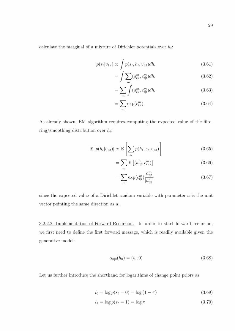
Figure 3.4. Randomly generated data from the generative model using

Dirichlet-Multinomial reset-observation models

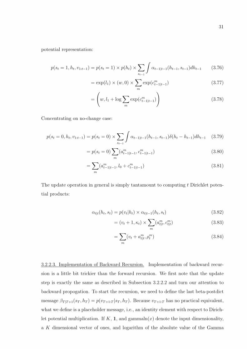
Figure 3.5. Forward filtered change point probabilities on forward-filtered mean

densities

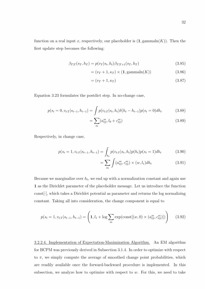
Figure 3.6. Backward-filtered change point probabilities on backward-filtered mean

densities

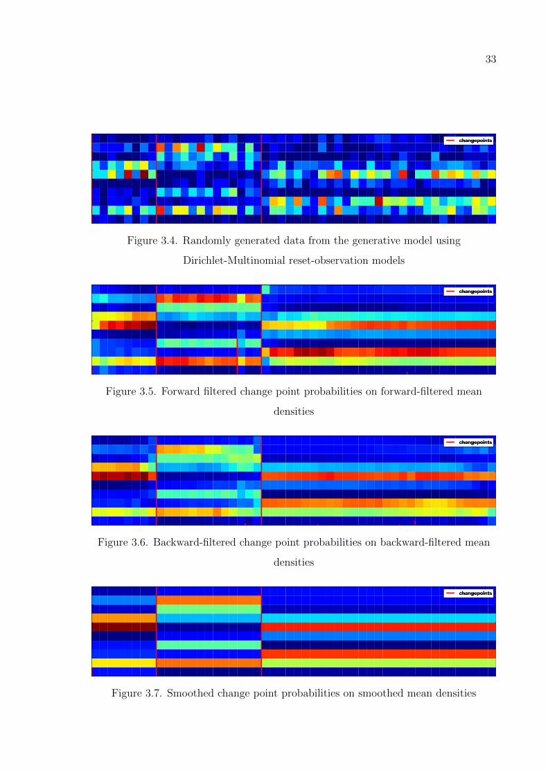
Figure 3.7. Smoothed change point probabilities on smoothed mean densities

34

the derivative of expected complete data log likelihood, given in Equation 3.36, with

respect to wk, k’th component of w, and set it equal to zero:

0 =T∑t=0

p(st = 1|v1:T , θ(τ))∂

∂wkEp(ht|v1:T ,θ(τ))

[logDir(ht;w)

](3.93)

=T∑t=0

p(st = 1|v1:T , θ(τ))Ep(ht|v1:T ,θ(τ))

[∂

∂wk

∑k

(wk − 1) log ht,k +∂

∂wklog Γ

(∑k

wk

)

− ∂

∂wk

∑k

log Γ(wk)

](3.94)

=T∑t=0

p(st = 1|v1:T , θ(τ))Ep(ht|v1:T ,θ(τ))

[log ht,k + ψ

(∑k

wk

)− ψ(wk)

](3.95)

=T∑t=0

p(st = 1|v1:T , θ(τ))

ψ

(∑k

wk

)− ψ(wk) + Ep(ht|v1:T ,θ(τ)) [log ht,k]

(3.96)

Here, ψ is known as the digamma function. If we set C =∑

t p(st = 1|v1:T , θ(τ)), above

expression becomes

1

C

T∑t=0

p(st = 1|v1:T , θ(τ))Ep(ht|v1:T ,θ(τ)) [log ht,k] = ψ(wk)− ψ

(∑k

wk

)(3.97)

Next, we need to compute the expectation, and hence need the posterior. If smoothed

posterior is expressed as below

p(ht|v1:T , θ(τ)) =1

Z

∑m

exp(cm)Dir(ht|am) (3.98)

where Z =∑

m exp(cm) is the normalization constant, then the expectation in Equa-

tion 3.97 can be explicitly written:

35

Ep(ht|v1:T ,θ(τ)) [log ht,k] =

∫p(ht|v1:T , θ(τ)) log ht,kdht (3.99)

=

∫1

Z

∑m

exp(cm)Dir(ht|am) log ht,kdht (3.100)

=1

Z

∑m

exp(cm)

∫Dir(ht|am) log ht,kdht (3.101)

=1

Z

∑m

exp(cm)E[log ht,k]p(ht|am) (3.102)

=1

Z

∑m

exp(cm) (ψ(amk )− ψ(am0 )) (3.103)

where we define am0 ≡∑

k amk and Minka shows how to compute the expectation in the

last step [35]. Plugging Equation 3.103 in Equation 3.97, we finally have the following:

1

C

T∑t=0

p(st = 1|v1:T , θ(τ))

(1

Z

∑m

exp(cm) (ψ(amk )− ψ(am0 ))

)= ψ(wk)− ψ

(∑k

wk

)(3.104)

Minka also shows that the following fixed-point iteration gives us the new estimate of

wk [35]:

ψ (wnewk )=

1

C

T∑t=0

p(st = 1|v1:T , θ(τ))

(1

Z

∑m

exp(cm) (ψ(amk )− ψ(am0 ))

)+ψ

(∑k

woldk

)(3.105)

Finally, ψ function must be inverted. Here, we do not give the details but a quickly

converging Newton iteration to perform the inversion is given in [35].

36

4. DDoS ATTACK DETECTION in SIP NETWORKS

In this chapter, we present an application of the Bayesian change point model

described in Chapter 3: DDoS attack detection in SIP networks. BCPM is a good

choice to tackle this problem because of two fundamental reasons. First, DDoS attacks

cause instantaneous changes in the quantities being observed, particularly in the net-

work traffic data. Furthermore, the problem naturally requires online data processing

rather than retrospective segmentation. It is worth pointing out that the model allows

us to formulate the inference problem in a batch settings as well, which typically results

in better performance.

Volumes of research that discuss a wide range of techniques for detecting (D)DoS

attacks have been produced. Some of the methods are problem-specific and hence

require incorporating the knowledge of the problem domain. On the other hand, sta-

tistical methods, relying heavily on learning the normal state of the observed system,

identify anomalies in general (rather than particular instances of DDoS attacks). Al-

though BCPM belongs to the second category, our application deals exclusively with

one type of DDoS attacks, namely flooding attacks, that target a particular network

protocol. Following subsections cover the details of flooding attacks and SIP networks.

We then describe our data generation mechanism and the data sets. The section is

concluded by the experiments conducted and the results.

4.1. SIP Networks

Voice Over the Internet Protocol (VoIP) technology has emerged as a strong al-

ternative to public switched telephone networks (PSTN) mainly because VoIP services

allow text and video communication in addition to the voice, and provide means for the

migration from PSTN. The transition from PSTN to VoIP leads to an increase in the

popularity of SIP [36]. Nowadays, SIP is considered to be one of the standard protocols

to setup, modify and end VoIP sessions. Two general types of SIP entities are (i)user

agents (UAs) and (ii)servers. A user agent is an endpoint entity that generates and

37

receives SIP messages. In a typical SIP session, UAs communicate with each other by

sending request and response messages. Servers are responsible for registering users,

storing their locations, delivering messages when needed and so forth.

SIP messages are divided into two basic categories: SIP requests and SIP re-

sponses. Each SIP request sent by a UA is supposed to be answered by one of the

corresponding SIP response messages. For example, a UA can make a REGISTER

request to the server in order to change its status to online, make an INVITE re-

quest to another UA to start a call, or make a BYE request to terminate an ongoing

conversation. A SIP response message generated for a request can be of one of the 6

SIP response categories: 1xx-provisional, 2xx-success, 3xx-redirection, 4xx-client error,

5xx-server error or 6xx-global failure.

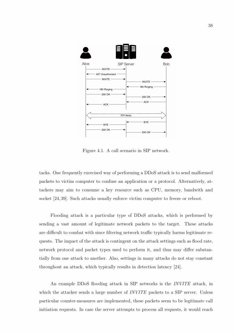
An illustrative example of SIP communication is given in Figure 4.1. It shows the

flow of exchanged messages between a server and two users during a normal call. In this

scenario, Alice initiates a call to Bob by sending an INVITE packet to the SIP server.

After authentication, the SIP server forwards this request to Bob. Similarly, Bob’s

response, in this case ACK packet showing that the call is accepted, is transmitted to

Alice through the SIP server. At the end, BYE messages terminate the conversation.

Once a SIP session is established, two endpoints start exchanging multimedia

data such as audio conversations, video streams, etc. Recall that SIP, being a signaling

protocol, is not involved in the multimedia data exchange between agents. Handshake

on the type of conversation, encoding, addresses and ports to be used for transfer and

other details regarding the data exchange are usually achieved using Session Description

Protocol [37]. Additionally, real-time media delivery relies on Real-time Transport

Protocol (RTP) [38].

4.2. DDoS Attacks

Denial of Service attacks intend to prevent legitimate use of a service. When

performed by multiple hosts, such attacks are called Distributed Denial of Service at-

38

Alice SIP Server Bob

RTP Media

INVITE

407 Unauthorized

INVITEINVITE

180 Ringing180 Ringing

200 OK200 OK

ACKACK

BYEBYE

200 OK200 OK

Figure 4.1. A call scenario in SIP network.

tacks. One frequently exercised way of performing a DDoS attack is to send malformed

packets to victim computer to confuse an application or a protocol. Alternatively, at-

tackers may aim to consume a key resource such as CPU, memory, bandwith and

socket [24,39]. Such attacks usually enforce victim computer to freeze or reboot.

Flooding attack is a particular type of DDoS attacks, which is performed by

sending a vast amount of legitimate network packets to the target. These attacks

are difficult to combat with since filtering network traffic typically harms legitimate re-

quests. The impact of the attack is contingent on the attack settings such as flood rate,

network protocol and packet types used to perform it, and thus may differ substan-

tially from one attack to another. Also, settings in many attacks do not stay constant

throughout an attack, which typically results in detection latency [24].

An example DDoS flooding attack in SIP networks is the INVITE attack, in

which the attacker sends a large number of INVITE packets to a SIP server. Unless

particular counter-measures are implemented, these packets seem to be legitimate call

initiation requests. In case the server attempts to process all requests, it would reach

39

its memory capacity and eventually stop responding to normal users.

4.3. Data Set Generation

Many machine learning algorithms proposed to sense DDoS attacks lack in pri-

vacy guarantees and may be exploited to uncover personal information, even from

anonymized data sets with the help of extra information [40]. Thus, in order to train

a machine learning solution, real world SIP traffic must be collected with uttermost

care in order not to reveal sensitive information. As expected, not many SIP data

sets are publicly available. To combat with the absence of real-world data, we build a

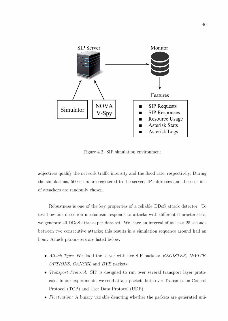
simulation setup that consists of following components:

• Simulator: To mimic the traffic on a SIP server, we build a probabilistic SIP

network simulation system that initiates calls between a number of users in real-

time [41]. The details of the underlying probabilistic model are presented in

Appendix A.

• Monitor: This module is responsible for collecting a set of features from a SIP

server. Collected data are delivered to a client computer in real time and DDoS

detection algorithm runs on streaming data.

• Trixbox: The simulation setup naturally requires a SIP server to operate. We

use Asterisk-based private branch exchange software named Trixbox as a SIP

server [42].

• NOVA V-Spy: To generate a rich variety of DDoS attacks concurrently with

normal traffic simulation, we make use of a commercial vulnerability scanning

tool, called NOVA V-Spy [43].

We control the simulation environment with two variables: network traffic in-

tensity and DDoS attack intensity. The former is a parameter of the Simulator and

controls the frequency of the calls whereas the latter is the rate of flooded packets,

governed by NOVA V-Spy. Both variables are binary, that is, they are set to be either

low or high, which makes up a total of four data sets. In the rest of this work, we refer

to the data sets as LOW-LOW, LOW-HIGH, HIGH-LOW and HIGH-HIGH, where the

40

Figure 4.2. SIP simulation environment

adjectives qualify the network traffic intensity and the flood rate, respectively. During

the simulations, 500 users are registered to the server. IP addresses and the user id’s

of attackers are randomly chosen.

Robustness is one of the key properties of a reliable DDoS attack detector. To

test how our detection mechanism responds to attacks with different characteristics,

we generate 40 DDoS attacks per data set. We leave an interval of at least 25 seconds

between two consecutive attacks; this results in a simulation sequence around half an

hour. Attack parameters are listed below:

• Attack Type: We flood the server with five SIP packets: REGISTER, INVITE,

OPTIONS, CANCEL and BYE packets.

• Transport Protocol: SIP is designed to run over several transport layer proto-

cols. In our experiments, we send attack packets both over Transmission Control

Protocol (TCP) and User Data Protocol (UDP).

• Fluctuation: A binary variable denoting whether the packets are generated uni-

41

formly with time or fluctuates over time.

• Content Size: NOVA V-Spy can optionally insert dummy strings to the end of

SIP messages. Because such strings affect the bandwidth consumption and thus

are relevant to attack detection task, we generate two sorts of DDoS attacks in

that manner: with or without dummy strings.

Even though there is no consensus on how to classify network traffic as abnormal,

the traffic caused by DDoS attacks is said to exhibit unique properties [44]. The main

source of information to establish whether the system is under attack or not is the

network load, which implies that significant changes in the pattern of SIP message

histograms possibly indicate a DDoS attack. Therefore, our first two feature categories

consist of 14 SIP Request (SReq) and 14 SIP Response (SRes) packets (the incoming

and outgoing packets) counted for fixed observation intervals (e.g., 1 sec).

We monitor three additional modules of the victim: Resource Usage (RU), Aste-

risk Stats (AS) and Asterisk Logs (AL). The first category is the pair of total CPU and

memory usage of the server. The second group consists of operating system statistics,

such as the number of open file handlers, connections, running threads, etc. The last

category counts the keywords in the log files generated by Asterisk. The listed features

are all expected to diverge from their settled values in case of an attack and hence

potentially signal it.

4.4. Evaluation Criteria

We measure the performances of different model specifications using precision (P)

and recall (R) measures. Both P and R are desired to be close to 1. As the rates of

false alarm and/or missed change points increase, P and R, respectively, diverge more

from 1. We also calculate the F-score (F), or the harmonic mean of precision and recall

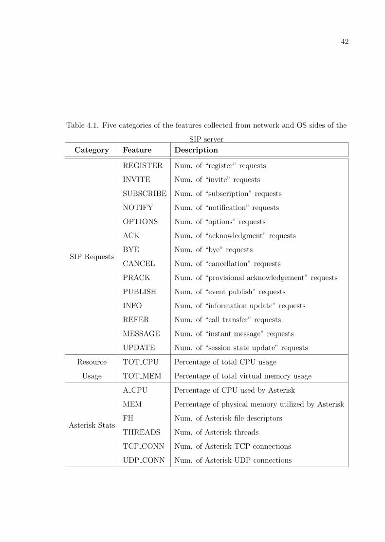
42

Table 4.1. Five categories of the features collected from network and OS sides of the

SIP server

Category Feature Description

SIP Requests

REGISTER Num. of “register” requests

INVITE Num. of “invite” requests

SUBSCRIBE Num. of “subscription” requests

NOTIFY Num. of “notification” requests

OPTIONS Num. of “options” requests

ACK Num. of “acknowledgment” requests

BYE Num. of “bye” requests

CANCEL Num. of “cancellation” requests

PRACK Num. of “provisional acknowledgement” requests

PUBLISH Num. of “event publish” requests

INFO Num. of “information update” requests

REFER Num. of “call transfer” requests

MESSAGE Num. of “instant message” requests

UPDATE Num. of “session state update” requests

Resource TOT CPU Percentage of total CPU usage

Usage TOT MEM Percentage of total virtual memory usage

Asterisk Stats

A CPU Percentage of CPU used by Asterisk

MEM Percentage of physical memory utilized by Asterisk

FH Num. of Asterisk file descriptors

THREADS Num. of Asterisk threads

TCP CONN Num. of Asterisk TCP connections

UDP CONN Num. of Asterisk UDP connections

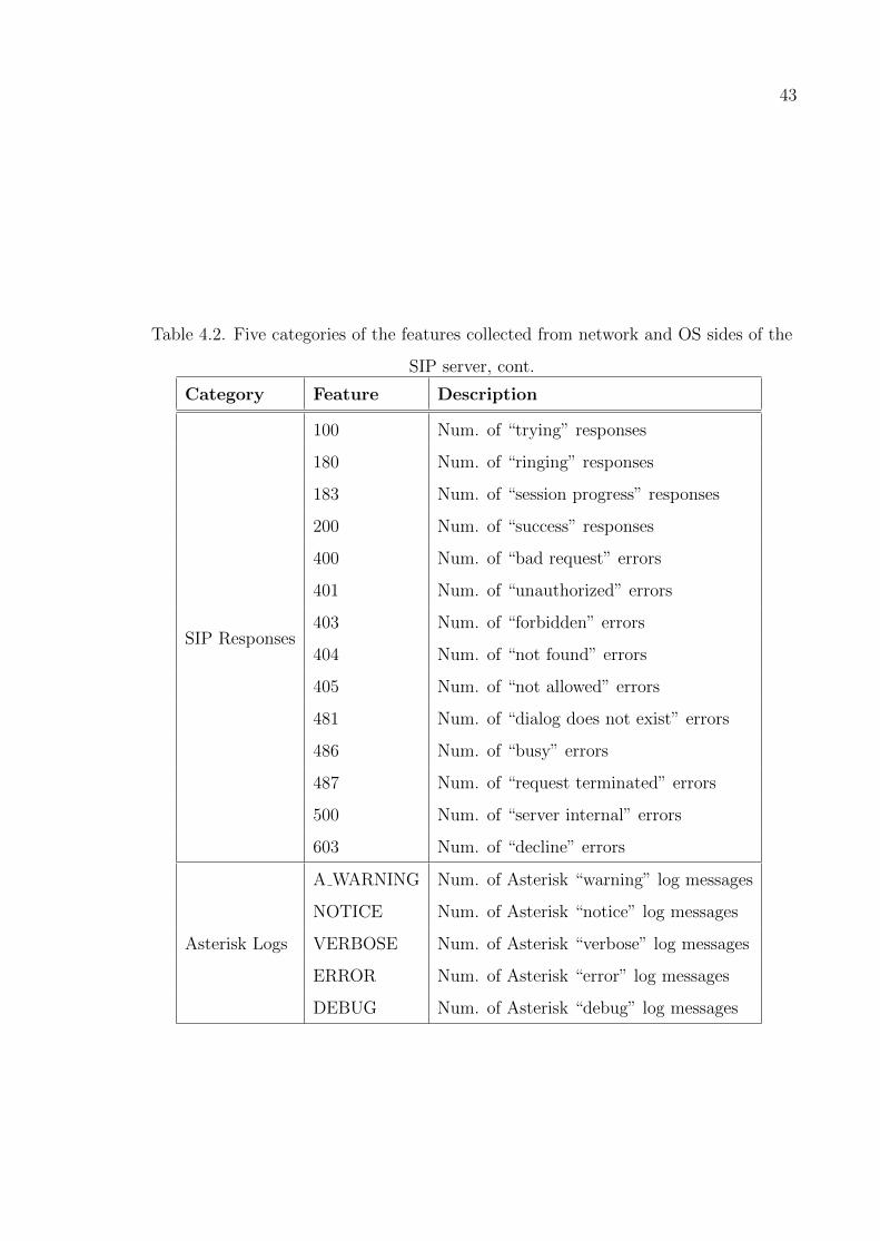
43

Table 4.2. Five categories of the features collected from network and OS sides of the

SIP server, cont.

Category Feature Description

SIP Responses

100 Num. of “trying” responses

180 Num. of “ringing” responses

183 Num. of “session progress” responses

200 Num. of “success” responses

400 Num. of “bad request” errors

401 Num. of “unauthorized” errors

403 Num. of “forbidden” errors

404 Num. of “not found” errors

405 Num. of “not allowed” errors

481 Num. of “dialog does not exist” errors

486 Num. of “busy” errors

487 Num. of “request terminated” errors

500 Num. of “server internal” errors

603 Num. of “decline” errors

Asterisk Logs

A WARNING Num. of Asterisk “warning” log messages

NOTICE Num. of Asterisk “notice” log messages

VERBOSE Num. of Asterisk “verbose” log messages

ERROR Num. of Asterisk “error” log messages

DEBUG Num. of Asterisk “debug” log messages

44

F -score = 2× P ×RP +R

(4.1)

Precision (P) =# true alarms

# alarms=

TaTa + Fa

(4.2)

Recall (R) =# true alarms

# ground truth=TaGa

(4.3)

where Ta and Fa are the true and false alarm counts respectively, and Ga is the true

number of change points. An alarm gt means signaling of a change event at time t,

which is triggered whenever the change point probability exceeds a certain threshold

λa. An alarm gt is said to be “correct” if it is signalled within ν seconds following

an attack onset at time t. In other words, we increment the number of true alarms

if 0 ≤ t − t < ν. Alarms not matched with any ground truth are regarded as false

positives.

4.5. Model and Parameter Settings

We conduct experiments with all models specificed in Subsection 3.1.5. For each

model, we either include or exclude a feature category, which makes a total of 25−1 = 31

sets of experiments per each model specification.

For a given feature setting and model, we perform a grid search in order to find the

hyperparameters yielding the best performance. Because the data sets are considerably

long and high-dimensional, each experiment is very time-consuming; therefore, we keep

the search space small. More concretely, we assign a single parameter φ for the Dirichlet

priors by setting wDM = [φ, φ, . . . , φ]. Similarly, we fix the shape parameter of all

Gamma priors in GP and Compound model to a single value ψ = wGP = wC and scale

parameter to 1. We also set π to three different values.

Parameter setting in Discrete model is slightly different. The first parameter to

be set is the number of states K. Regardless of this value, we assume that the prior

distribution over hidden states to be flat: wD = 1/K[1, 1, . . . , 1]. In order to determine

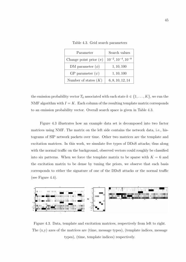
45

Table 4.3. Grid search parameters

Parameter Search values

Change point prior (π) 10−2, 10−4, 10−8

DM parameter (φ) 1, 10, 100

GP parameter (ψ) 1, 10, 100

Number of states (K) 6, 8, 10, 12, 14

the emission probability vector Tk associated with each state k ∈ 1, . . . , K, we run the

NMF algorithm with I = K. Each column of the resulting template matrix corresponds

to an emission probability vector. Overall search space is given in Table 4.3.

Figure 4.3 illustrates how an example data set is decomposed into two factor

matrices using NMF. The matrix on the left side contains the network data, i.e., his-

tograms of SIP network packets over time. Other two matrices are the template and

excitation matrices. In this work, we simulate five types of DDoS attacks; thus along

with the normal traffic on the background, observed vectors could roughly be classified

into six patterns. When we force the template matrix to be sparse with K = 6 and

the excitation matrix to be dense by tuning the priors, we observe that each basis

corresponds to either the signature of one of the DDoS attacks or the normal traffic

(see Figure 4.4).

!

Figure 4.3. Data, template and excitation matrices, respectively from left to right.

The (x,y) axes of the matrices are (time, message types), (template indices, message

types), (time, template indices) respectively.

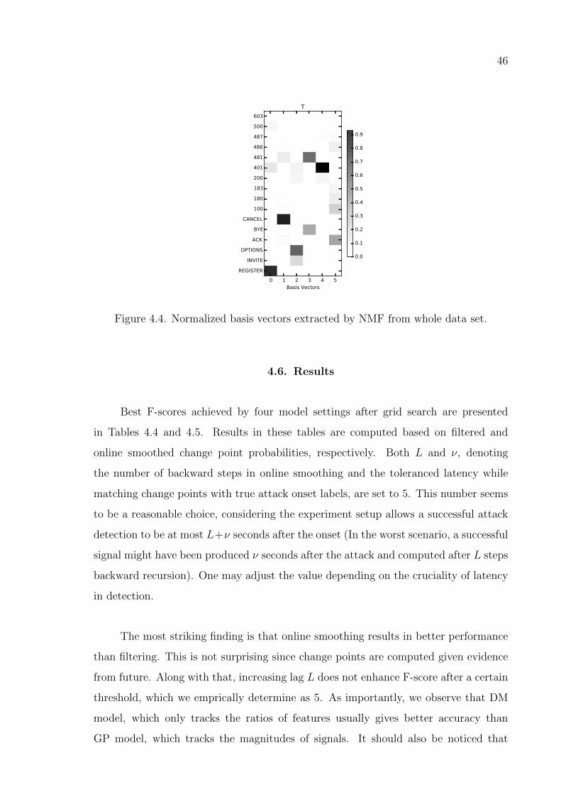
46

0 1 2 3 4 5

Basis Vectors

603

500

487

486

481

401

200

183

180

100

CANCEL

BYE

ACK

OPTIONS

INVITE

REGISTER

T

0.0

0.1

0.2

0.3

0.4

0.5

0.6

0.7

0.8

0.9

Figure 4.4. Normalized basis vectors extracted by NMF from whole data set.

4.6. Results

Best F-scores achieved by four model settings after grid search are presented

in Tables 4.4 and 4.5. Results in these tables are computed based on filtered and

online smoothed change point probabilities, respectively. Both L and ν, denoting

the number of backward steps in online smoothing and the toleranced latency while

matching change points with true attack onset labels, are set to 5. This number seems

to be a reasonable choice, considering the experiment setup allows a successful attack

detection to be at most L+ν seconds after the onset (In the worst scenario, a successful

signal might have been produced ν seconds after the attack and computed after L steps

backward recursion). One may adjust the value depending on the cruciality of latency

in detection.

The most striking finding is that online smoothing results in better performance

than filtering. This is not surprising since change points are computed given evidence

from future. Along with that, increasing lag L does not enhance F-score after a certain

threshold, which we emprically determine as 5. As importantly, we observe that DM

model, which only tracks the ratios of features usually gives better accuracy than

GP model, which tracks the magnitudes of signals. It should also be noticed that

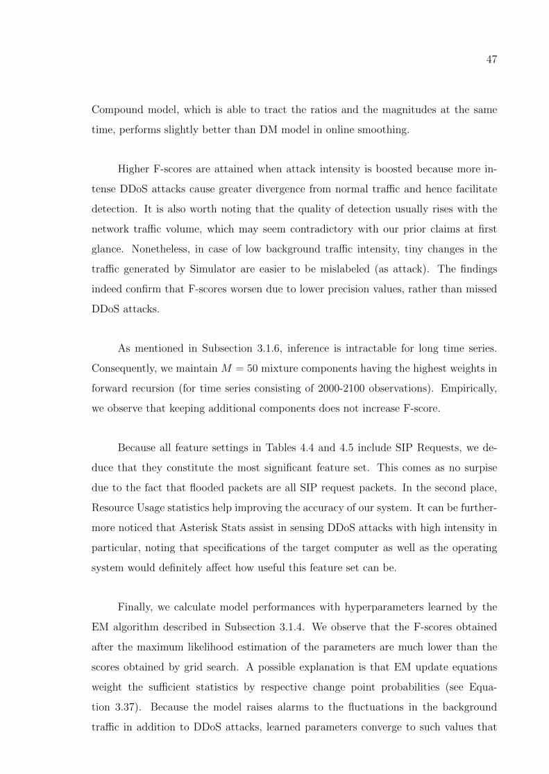
47

Compound model, which is able to tract the ratios and the magnitudes at the same

time, performs slightly better than DM model in online smoothing.

Higher F-scores are attained when attack intensity is boosted because more in-

tense DDoS attacks cause greater divergence from normal traffic and hence facilitate

detection. It is also worth noting that the quality of detection usually rises with the

network traffic volume, which may seem contradictory with our prior claims at first

glance. Nonetheless, in case of low background traffic intensity, tiny changes in the

traffic generated by Simulator are easier to be mislabeled (as attack). The findings

indeed confirm that F-scores worsen due to lower precision values, rather than missed

DDoS attacks.

As mentioned in Subsection 3.1.6, inference is intractable for long time series.

Consequently, we maintain M = 50 mixture components having the highest weights in

forward recursion (for time series consisting of 2000-2100 observations). Empirically,

we observe that keeping additional components does not increase F-score.

Because all feature settings in Tables 4.4 and 4.5 include SIP Requests, we de-

duce that they constitute the most significant feature set. This comes as no surpise

due to the fact that flooded packets are all SIP request packets. In the second place,

Resource Usage statistics help improving the accuracy of our system. It can be further-

more noticed that Asterisk Stats assist in sensing DDoS attacks with high intensity in

particular, noting that specifications of the target computer as well as the operating

system would definitely affect how useful this feature set can be.

Finally, we calculate model performances with hyperparameters learned by the

EM algorithm described in Subsection 3.1.4. We observe that the F-scores obtained

after the maximum likelihood estimation of the parameters are much lower than the

scores obtained by grid search. A possible explanation is that EM update equations

weight the sufficient statistics by respective change point probabilities (see Equa-

tion 3.37). Because the model raises alarms to the fluctuations in the background

traffic in addition to DDoS attacks, learned parameters converge to such values that

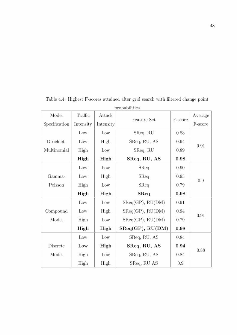
48

Table 4.4. Highest F-scores attained after grid search with filtered change point

probabilities

Model Traffic AttackFeature Set F-score

Average

Specification Intensity Intensity F-score

Low Low SReq, RU 0.83

0.91Dirichlet- Low High SReq, RU, AS 0.94

Multinomial High Low SReq, RU 0.89

High High SReq, RU, AS 0.98

Low Low SReq 0.90

0.9Gamma- Low High SReq 0.93

Poisson High Low SReq 0.79

High High SReq 0.98

Low Low SReq(GP), RU(DM) 0.91

0.91Compound Low High SReq(GP), RU(DM) 0.94

Model High Low SReq(GP), RU(DM) 0.79

High High SReq(GP), RU(DM) 0.98

Low Low SReq, RU, AS 0.84

0.88Discrete Low High SReq, RU, AS 0.94

Model High Low SReq, RU, AS 0.84

High High SReq, RU AS 0.9

49

Table 4.5. Highest F-scores attained after grid search with online smoothed change

point probabilities

Model Traffic AttackFeature Set F-score

Average

Specification Intensity Intensity F-score

Low Low SReq 0.92

0.95Dirichlet- Low High SReq, RU, AS 0.96

Multinomial High Low SReq, RU 0.92

High High SReq, RU, AS 0.98


0.93Gamma- Low High SReq, RU 0.95

Poisson High Low SReq, RU 0.89

High High SReq, RU 0.94

Low Low SReq(GP), AS(DM) 0.95

0.96Compound Low High SReq(GP), AS(DM) 0.96

Model High Low SReq(DM), RU(GP) 0.94

High High SReq(GP), AS(DM) 0.99


0.9Discrete Low High SReq, AS 0.94

Model High Low SReq, RU 0.84

High High SReq, AS 0.92

50

eventually make the model more sensitive to the fluctuations, whereas we would like

to detect DDoS attack onsets only.

51

5. CONCLUSION

In this work, we approached the change point detection problem from a Bayesian

standpoint. Our model is a hierarchical hidden Markov model that comprises three sets

of variables: switches, latent dynamics and observations. Our formulation reduces the

task of deciding whether a change occurs or not at a given time to computing the pos-

terior probability of the switch variable at that time. We provided a forward-backward

type algorithm for inference, which allows both real-time and batch processing. We

also derived update equations for learning two model parameters, namely, the prior

probability of a change and reset parameter, through the Expectation-Maximization

algorithm.

We described our change point detection framework independent of particular

distributions modeling observations and latent dynamics. To specify the model, we

explained four different observation and reset distribution pairs: Gamma-Poisson,

Dirichlet-Multinomial, Compound and Discrete models, which track the magnitude,

ratio, a mixture of magnitude and ratio of the input signal, and the discrete states

of the observed system. Section 3.2 presented an exhaustive analysis of the Dirichlet-

Multinomial model, in which forward-backward messages and the predict and update

equations were explicitly derived. We also discussed the complexity analysis and a

simple trick that allows real-time approximate inference.

The novel application of the model is DDoS attack detection in SIP networks.

Since we were not able to find any publicly available data set collected from a SIP server

under a DDoS attack, we first built a simulation environment consisting of a SIP traffic

generator, SIP server and DDoS attack generator. We conducted several experiments

with different model specifications and feature combinations, and showed that the

Compound model outperforms the others. Moreover, we identified SIP Request and

Resource Usage feature categories as the most informative ones as they very frequently

appear in the settings yielding the highest F-scores.

52

As we demonstrated in our experiments, the proposed method is powerful and

flexible, and yields good results in an arguably challenging problem. Nonetheless, both

the model and the applications can be further improved in many respects. A list of

future research directions are as follows:

• Despite pruning is shown to work very well in practice, other approximation

techniques such as particle filters or collapsing multiple components into a single

one may be investigated for problems involving highly heterogeneous time series

data.

• Currently, the switch variables are assumed to be independent of all other vari-

ables in the model. A Markov chain on the switches may be considered.

• The latent dynamics when there is no change do not necessarily stay the same.

New transition dynamics could be explored.

• We can build a more generic framework if multiple reset templates are allowed

to exist. Such a setup would better represent the uncertainty over the latent

dynamics.

• New observation-reset distribution pairs may be worked out. As long as the reset

distribution is the conjugate prior for the observation distribution, the generic

inference and parameter learning recipes stay valid.

53

REFERENCES

1. Carlin, B. P., A. E. Gelfand and A. F. M. Smith, “Hierarchical Bayesian

Analysis of Changepoint Problems”, Journal of the Royal Statistical So-

ciety. Series C (Applied Statistics), Vol. 41, No. 2, pp. 389–405, 1992,

http://www.jstor.org/stable/2347570.

2. Caron, F., A. Doucet and R. Gottardo, “On-line changepoint detection and pa-

rameter estimation with application to genomic data”, Statistics and Computing ,

Vol. 22, No. 2, pp. 579–595, 2012.

3. Aroian, L. A. and H. Levene, “The effectiveness of quality control charts”, Journal

of the American Statistical Association, Vol. 45, No. 252, pp. 520–529, 1950.

4. Bormetti, G., M. E. De Giuli, D. Delpini and C. Tarantola, “Bayesian value-at-risk

with product partition models”, Quantitative Finance, Vol. 12, No. 5, pp. 769–780,

2012.

5. Barlow, J., O. Creutzfeldt, D. Michael, J. Houchin and H. Epelbaum, “Automatic

adaptive segmentation of clinical EEGs”, Electroencephalography and Clinical Neu-

rophysiology , Vol. 51, No. 5, pp. 512–525, 1981.

6. Bodenstein, G. and H. M. Praetorius, “Feature extraction from the electroen-

cephalogram by adaptive segmentation”, Proceedings of the IEEE , Vol. 65, No. 5,

pp. 642–652, 1977.

7. Erdman, C. and J. W. Emerson, “A fast Bayesian change point analysis for the

segmentation of microarray data”, Bioinformatics , Vol. 24, No. 19, pp. 2143–2148,

2008.

8. Braun, J. V., R. Braun and H.-G. Muller, “Multiple changepoint fitting via quasi-

likelihood, with application to DNA sequence segmentation”, Biometrika, pp. 301–

54

314, 2000.

9. Zhang, H., Z. Gu, C. Liu and T. Jie, “Detecting VoIP-specific Denial-of-service

Using Change-point Method”, Proceedings of the 11th International Conference

on Advanced Communication Technology - Volume 2 , pp. 1059–1064, IEEE Press,

2009.

10. Rebahi, Y. and D. Sisalem, “Change-point detection for voice over IP denial of

service attacks”, KiVS 2007 , 2007.

11. Nyamundanda, G., A. Hegarty and K. Hayes, “Product partition latent variable

model for multiple change-point detection in multivariate data”, Journal of Applied

Statistics , Vol. 42, No. 11, pp. 2321–2334, 2015.

12. Basseville, M., I. V. Nikiforov et al., Detection of abrupt changes: theory and

application, Vol. 104, Prentice Hall Englewood Cliffs, 1993.

13. Desobry, F., M. Davy and C. Doncarli, “An online kernel change detection algo-

rithm”, IEEE Transactions on Signal Processing , Vol. 53, No. 8, pp. 2961–2974,

2005.

14. Kawahara, Y., T. Yairi and K. Machida, “Change-point detection in time-series

data based on subspace identification”, Data Mining, 2007. ICDM 2007. Seventh

IEEE International Conference on, pp. 559–564, IEEE, 2007.

15. Gupta, V., “Speaker change point detection using deep neural nets”, Acoustics,

Speech and Signal Processing (ICASSP), 2015 IEEE International Conference on,

pp. 4420–4424, IEEE, 2015.

16. Bulunga, M. L., “Change-point detection in dynamical systems using auto-

associative neural networks”, , 2012.

17. Xuan, X. and K. Murphy, “Modeling changing dependency structure in multi-

55

variate time series”, Proceedings of the 24th international conference on Machine

learning , pp. 1055–1062, ACM, 2007.

18. Stephens, D., “Bayesian retrospective multiple-changepoint identification”, Applied

Statistics , pp. 159–178, 1994.

19. Chib, S., “Calculating posterior distributions and modal estimates in Markov mix-

ture models”, Journal of Econometrics , Vol. 75, No. 1, pp. 79–97, 1996.

20. Chib, S., “Estimation and comparison of multiple change-point models”, Journal

of econometrics , Vol. 86, No. 2, pp. 221–241, 1998.

21. Fearnhead, P., “Exact and efficient Bayesian inference for multiple changepoint

problems”, Statistics and computing , Vol. 16, No. 2, pp. 203–213, 2006.

22. Barry, D. and J. A. Hartigan, “Product partition models for change point prob-

lems”, The Annals of Statistics , pp. 260–279, 1992.

23. Adams, R. P. and D. J. MacKay, “Bayesian online changepoint detection”, arXiv

preprint arXiv:0710.3742 , 2007.

24. Mirkovic, J. and P. Reiher, “A taxonomy of DDoS attack and DDoS defense mech-

anisms”, ACM SIGCOMM Computer Communications Review , Vol. 34, No. 2, pp.

39–53, 2004.

25. Yıldız, C., B. Kurt and T. Y. Ceritli, “Bayesian Change Point Model”,

github.com/pilab-sigma/bcpm, 2013, [Online; accessed 4-July-2017].

26. Dempster, A. P., N. M. Laird and D. B. Rubin, “Maximum likelihood from incom-

plete data via the EM algorithm”, Journal of the royal statistical society. Series B

(methodological), pp. 1–38, 1977.

27. McLachlan, G. and T. Krishnan, The EM algorithm and extensions , Vol. 382, John

Wiley & Sons, 2007.

56

28. Kullback, S. and R. A. Leibler, “On information and sufficiency”, The annals of

mathematical statistics , Vol. 22, No. 1, pp. 79–86, 1951.

29. Lee, D. D. and H. S. Seung, “Learning the parts of objects by non-negative matrix

factorization.”, Nature, Vol. 401, pp. 788–91, 1999.

30. Cemgil, A. T., “Bayesian inference for nonnegative matrix factorisation models”,

Computational Intelligence and Neuroscience, Vol. 2009, 2009.

31. Schmidt, M. N., O. Winther and L. K. Hansen, “Bayesian non-negative matrix

factorization”, International Conference on Independent Component Analysis and

Signal Separation, pp. 540–547, Springer, 2009.

32. Barber, D., Bayesian Reasoning and Machine Learning , Cambridge University

Press, New York, NY, USA, 2012.

33. Barber, D. and A. T. Cemgil, “Graphical models for time-series”, Signal Processing

Magazine, IEEE , Vol. 27, No. 6, pp. 18–28, 2010.

34. Bracegirdle, C. and D. Barber, “Switch-Reset Models : Exact and Ap-

proximate Inference”, G. J. Gordon and D. B. Dunson (Editors), Pro-

ceedings of the Fourteenth International Conference on Artificial Intelli-

gence and Statistics (AISTATS-11), Vol. 15, pp. 190–198, Journal of Ma-

chine Learning Research - Workshop and Conference Proceedings, 2011,

http://proceedings.mlr.press/v15/bracegirdle11a.html.

35. Minka, T., Estimating a Dirichlet distribution, Tech. rep., 2000,

https://tminka.github.io/papers/dirichlet/minka-dirichlet.pdf.

36. Rosenberg, J., H. Schulzrinne, G. Camarillo, A. Johnston, J. Peterson, R. Sparks,

M. Handley and S. E, RFC 3261: SIP: Session Initiation Protocol , Tech. rep.,

IETF, 2002, www.ietf.org/rfc/rfc3261.txt.

57

37. Handley, M. and V. Jacobson, “SDP: Session Description Protocol”, , 1998.

38. Schulzrinne, H., S. Casner, R. Frederick and V. Jacobson, “RTP: A Transport

Protocol for Real-Time Applications”, , 2003.

39. Zargar, S. T., J. Joshi and D. Tipper, “A survey of defense mechanisms against dis-

tributed denial of service (DDoS) flooding attacks”, IEEE communications surveys

& tutorials , Vol. 15, No. 4, pp. 2046–2069, 2013.

40. Narayanan, A. and V. Shmatikov, “Robust de-anonymization of large sparse

datasets”, 2008 IEEE Symposium on Security and Privacy (sp 2008), pp. 111–

125, IEEE, 2008.

41. Kurt, B., C. Yıldız, Y. T. Ceritli, M. Yamac, M. Semerci, B. Sankur and A. T.

Cemgil, “A Probabilistic SIP Network Simulation System”, 24th IEEE Conference

on Signal Processing and Communications Applications (Accepted, in Turkish),

2016.

42. “Trixbox”, http://www.fonality.com/trixbox, 2016, [Online; accessed 29-April-

2016].

43. “Nova V-SPY”, http://www.netas.com.tr/en/, 2016, [Online; accessed 29-April-

2016].

44. Xu, Y. and R. Guerin, “On the robustness of router-based denial-of-service (DoS)

defense systems”, ACM SIGCOMM Computer Communication Review , Vol. 35,

No. 3, pp. 47–60, 2005.

45. Goldenberg, A., A. X. Zheng, S. E. Fienberg and E. M. Airoldi, “A Survey of

Statistical Network Models”, Foundations and Trends in Machine Learning , Vol. 2,

No. 2, pp. 129–233, 2010.

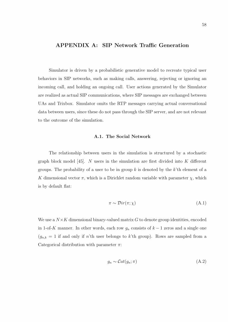
58

APPENDIX A: SIP Network Traffic Generation

Simulator is driven by a probabilistic generative model to recreate typical user

behaviors in SIP networks, such as making calls, answering, rejecting or ignoring an

incoming call, and holding an ongoing call. User actions generated by the Simulator

are realized as actual SIP communications, where SIP messages are exchanged between

UAs and Trixbox. Simulator omits the RTP messages carrying actual conversational

data between users, since these do not pass through the SIP server, and are not relevant

to the outcome of the simulation.

A.1. The Social Network

The relationship between users in the simulation is structured by a stochastic

graph block model [45]. N users in the simulation are first divided into K different

groups. The probability of a user to be in group k is denoted by the k’th element of a

K dimensional vector π, which is a Dirichlet random variable with parameter χ, which

is by default flat:

π ∼ Dir(π;χ) (A.1)

We use aN×K dimensional binary-valued matrixG to denote group identities, encoded

in 1-of-K manner. In other words, each row gn consists of k− 1 zeros and a single one

(gn,k = 1 if and only if n’th user belongs to k’th group). Rows are sampled from a

Categorical distribution with parameter π:

gn ∼ Cat(gn; π) (A.2)

59

A.2. Phone Books

First, a phone book bn is generated for each user n to determine persons that the

user is most likely to call. bn is a vector of length N such that bn,m is the probability

of user n calling user m whenever it decides to make a call. This vector is drawn from

a Dirichlet distribution with a parameter αn that is specific to each user.

bn ∼ Dir(bn;αn) (A.3)

All entries except for n’th one of αn ∈ RN are 1, and αn,n = 0. This means the phone

book bn is drawn from an (almost) flat Dirichlet distribution, but bn itself is not flat.

Each user n has different probabilities of calling other users.

Whenever user n decides to make a call, it selects a user c from its phone book to call

from a Categorical distribution

c ∼ Cat(c; bn) (A.4)

A.3. Registration

When the simulation starts, all users are offline. The amount of time user n

spends before registration is denoted by rn and generated as follows:

rn ∼ G(rn; 2, 10) (A.5)

Furthermore, each user n sends a re-register packet with a fixed period tn that is again

sampled from Gamma distribution:

tn ∼ G(tn; 30, 10) (A.6)

60

A.4. Call Rates

The rate of phone calls for each user n is determined by βn, which is generated

from Gamma distribution:

βn ∼ G(βn;µ, 10) (A.7)

During the simulation, whenever user n becomes idle, it waits for a random in seconds,

which is drawn from Exponential distribution with rate βn.

in ∼ Exp(in; βn) (A.8)

Exp(in|βn) = 1/βn exp(−in/βn) (A.9)

To generate low traffic, we set µ to 20 and µ = 5 in case of high traffic.

A.5. Call Durations

Each user n has its own average call duration δn, drawn from Uniform distribution:

δn ∼ U(δn; 20, 200) (A.10)

Some users tend to make short calls, while others prefer to talk longer. Whenever

a call is set up between users n and m, they both sample the duration of the call

independently and the one who wants to talk shorter hangs up. Therefore, we generate

a call duration dn,m as follows

dn|δn ∼ Exp(dn; δn) (A.11)

dm|δm ∼ Exp(dm; δm) (A.12)

dn,m = min(dn, dm) (A.13)

61

A.6. Call Responses

Every user n is associated with a call answering probability an and call holding

probability hn. We draw them from following uniform priors:

an ∼ U(an; 0.8, 1) (A.14)

hn ∼ U(hn; 0, 0.1) (A.15)

Whenever a user in available state receives a call, we draw a Bernoulli variable xn

with parameter an for the decision. The call is accepted if xn = 1. If the user is

already talking when she receives the call, we draw another binary random variable zn

with parameter hn. If zn turns out to be 1, she holds the other party and accepts the

incoming call. Otherwise, incoming call is rejected.

xn ∼ BE(xn; an) (A.16)

zn ∼ BE(zn;hn) (A.17)

The actions that users take for incoming calls is given in Figure A.1.

62

User A calls user B

if B.status == “Available” then

generate x ∈ U [0, 1)

if x ≤ B.answering probability then

return “ACCEPT”

else

return “REJECT”

end if

else

generate z ∈ U [0, 1)

if z ≤ B.holding probability then

return “HOLD OTHER PARTY”

else

return “BUSY”

end if

end if

Figure A.1. Algorithm to generate responses to calls

INFERENCE AND PARAMETER ESTIMATION IN bycagatayyildiz.github.io/pdf/msc_thesis.pdf · INFERENCE AND...

Documents

Transcript of INFERENCE AND PARAMETER ESTIMATION IN bycagatayyildiz.github.io/pdf/msc_thesis.pdf · INFERENCE AND...