Inequality and Democratization: Individual-Level Evidence ...
34
Inequality and Democratization: Individual-Level Evidence of Preferences for Redistribution under Autocracy Ben Ansell and David Samuels University of Minnesota While some research has explored the relationship between individual income and demand for redistribution under democracy--finding little support for median-voter theories of redistribution- -no research has explored this relationship under autocracy, even though this connection is a crucial assumption of redistributivist theories of democratization (Boix 2003; Acemoglu and Robinson 2006). We explore the relationship between individual income and support for redistributive government policies in autocratic societies using micro-level data from the World Values Surveys, finding no empirical support for the core assumption of median-voter models that regime change is a function of elites’ fear of the redistributive demands of the poor. We thank Kevin Lucas for research assistance. This paper is part of a larger book-length project, please do not cite without permission. 1. Introduction
Transcript of Inequality and Democratization: Individual-Level Evidence ...

Inequality and Democratization: Individual-Level Evidence of Preferences for Redistribution under Autocracy
Ben Ansell and David Samuels
University of Minnesota
While some research has explored the relationship between individual income and demand for redistribution under democracy--finding little support for median-voter theories of redistribution--no research has explored this relationship under autocracy, even though this connection is a crucial assumption of redistributivist theories of democratization (Boix 2003; Acemoglu and Robinson 2006). We explore the relationship between individual income and support for redistributive government policies in autocratic societies using micro-level data from the World Values Surveys, finding no empirical support for the core assumption of median-voter models that regime change is a function of elites’ fear of the redistributive demands of the poor.
We thank Kevin Lucas for research assistance. This paper is part of a larger book-length project, please do not cite without permission. 1. Introduction

2
The gospel of political economy preaches that extending the franchise leads to greater
government redistribution. Faith in this tenet is rooted in the intuitive contrast between
autocracies, which restrict effective participation to the wealthy few, and democracies, which
allow the poor greater voice. Because there are always more poor people than rich people
franchise expansion should lower the income of the average voter. And if we assume that voters
support policies that maximize their welfare, then universal suffrage should raise demand for
redistribution of wealth. Moreover, such demand should increase with the level of societal
inequality—as the rich grow richer and the poor grow poorer, pressures for redistributive policies
should grow more intense.
The syllogism between political and economic equality has dominated the fears and the
hopes attached to democracy ever since in the inception of representative government. Those on
the right have long worried that political equality would threaten property—and likewise, those
on the left remained skeptical that acquisition of political rights alone would satisfy those on the
bottom of the economic ladder--by Marx’s time, the idea had spread that “democracy in the
political realm must naturally lead to social and economic equality” (Przeworski 2010, 303).
Vast socioeconomic inequalities persist in democracies around the world. Indeed, in
developed democracies the gap between rich and poor has grown wider in recent decades. Still,
the belief that democracy and property are in tension remains rock-solid, and the seductiveness
of the median-voter model of political economy has helped cement this faith. Meltzer and
Richard’s (1981) formalization of the redistributive model of electoral politics sparked an
avalanche of research seeking to explain cross-national variation in patterns of social-welfare
spending. Surprisingly, given the intuitive nature of the model, results have consistently called
into question the gospel truth that pressures for redistribution increase with inequality (see e.g.
3
Bartels 2008; Roemer 2001: Moene and Wallerstein 2003; Iversen and Soskice 2006; Kenworthy
and McCall 2007). Scholars have repeatedly found that democracies redistribute far less than
they “should”--yet have proven unwilling to abandon the Meltzer-Richard (MR) model, leading
Adam Przeworski (2010, 85) to sardonically call it “political economists’ favorite toy.”
The shaky empirical results in support of the median-voter model call into question its
theoretical utility. Yet despite weak results, faith in the syllogism equating democracy and
redistribution remains so strong that even though MR did not devise their model to apply in non-
democratic contexts, Acemoglu and Robinson (2000, 2006) and Boix (2003) have developed
“redistributivist” models of regime change, applying the MR rational expectations logic to
explain transitions to democracy. Simplifying greatly, the logic of these models is as follows:
“Everyone—from the incumbent dictator down to the lowliest of peasants--knows that under
democracy the poor will soak the rich. So, incumbent elites will be reluctant to democratize to
begin with, but their reluctance depends fundamentally on what kind of assets there are (fixed or
mobile) and how those assets are distributed within society. All else equal, the distribution of
wealth impacts the likelihood of regime change.”
The utility of redistributivist models of regime change depends crucially on the
descriptive and predictive accuracy of this underlying theoretical assumption about actors’
preferences—that the median voter prefers a political arrangement that will maximize
redistribution, and that such preferences intensify as societal inequality increases. To the extent
that the MR model holds up to empirical scrutiny, we gain confidence that the underlying
assumption is useful for thinking about actors’ preferences in cases of regime transition. To the
extent that it does not, then we have good reason to question the assumption that fear of the poor

4
drives elites’ strategies in cases of regime change—and better reason to accept an alternative
understanding of regime change.
Elsewhere, we test the implication of redistributivist models of regime change that
transitions to democracy are at least partly a function of economic inequality, advancing a
“contractarian” theoretical model (Ansell and Samuels 2010a) and showing that neither Boix’s
(2003) nor Acemoglu and Robinson’s (2006) “redistributivist” arguments accurately predict
regime transitions. In a separate paper (Ansell and Samuels 2010b) we show, using data from
1880 to 1930 that in the late nineteenth and early twentieth centuries there is little evidence that
democracies did indeed redistribute more than did autocracies.
In this paper we add another layer to our theoretical and empirical critique of
redistributivist models of regime change, by assessing the predictions of the MR median-voter
hypothesis that demand for redistribution should decline with individual income but rise with
societal inequality. A few papers have explored this question using micro-level data: Finseraas
(2008) claims to find evidence supporting the MR conjecture, but others find no relationship
between inequality, income, and the median voter’s preferences over redistribution (Kenworthy
and McCall 2007; Lübker 2007; Huber and Stanig 2009).
What is novel about this paper is that we consider the impact of income and inequality on
demand for redistributive spending in autocracies. Although the rational-expectations logic of
the MR model was designed to apply under universal suffrage, Boix and Acemoglu and
Robinson assume that the mechanisms of the model do not differ where elections do not exist, or
are non-competitive. Given this, using data from autocratic societies is the appropriate way to
test the strength of redistributivist models of regime change.

5
Our results offer further reason for skepticism about the theoretical and empirical utility
the Meltzer-Richard model and its extensions as applied to the study of democratization. Were
the MR model correct--and were Boix’s and Acemoglu and Robinson’s extensions of that model
correct--we would expect to see a positive relationship between inequality and demand for
redistribution under autocracy. However, our findings completely confound the MR model: we
find a significant negative relationship between inequality and demand for redistribution in
cross-national perspective. This result helps solve the puzzle of why empirical support for the
MR model is so weak: quite simply, the median voter does not demand greater redistribution as
inequality increases. The next section discusses competing hypotheses; empirics follow.
2. Theoretical Discussion
The starting point for many explorations of the relationship between politics and
economics is the assumption that voters’ preferences depend heavily on their income. Do
citizens’ attitudes fit with this simple assumption? Relatively little research explores the median-
voter model at the individual level. Instead, most research uses aggregate-level data—for
example, societal-level inequality and aggregate government spending levels—taking as given
the underlying micro-level hypothesis that voters’ preferences about redistribution are a function
of their income and of overall societal inequality.
More pertinently, the central assumption of the MR model--that elites’ and masses’
preferences over redistribution shape their political behavior --has never been tested in non-
democratic regimes. In their adaptations of the MR model, both Boix (2003) and Acemoglu and
Robinson (2006) assume that (a) the poor prefer more income redistribution than prevails under
autocracy and that the rich prefer the distribution of income under autocracy to that under

6
democracy (all else equal); and (b) that the difference in preferences between rich and poor over
redistribution widens with societal inequality.
The distinction between Boix’s linear model of democratization and Acemoglu and
Robinson’s ‘inverse-U’ hypothesis depends on political mechanisms--such as the possibility of
revolution by the poor or repression by the rich--that are causally exogenous to individual-level
preferences. Such mechanisms are irrelevant when we examine only individual-level preferences
over the distribution of income. Accordingly, if the MR hypotheses as applied in autocracies
were true, we should expect poorer people to be more desirous of income redistribution and less
tolerant of income inequalities than rich citizens. We should also expect the intensity of such
preferences to increase where inequality is higher. Let us elaborate the redistributivist hypotheses
more specifically:
• H1: Holding societal inequality constant, as an individual’s income goes up, his or her
demand for redistribution should go down.
• H2: Holding individual income constant, the ‘democratic median voter’ (i.e. the person
with median income among all those who would be eligible to vote in democracy) will
desire higher redistribution as societal inequality goes up.
• H3: H1 and H2 are interactive: The negative relationship between individual income and
demand for redistribution should intensify as societal inequality increases – that is, the
poor’s preference for redistribution will intensify, as will opposition by the rich.
The first hypothesis is an essential underlying assumption of the Meltzer-Richard model
– that demand for redistribution is decreasing in income. A basic test of this hypothesis can be
done on individual-level data without reference to any national context. The second hypothesis is
a core implication of the Meltzer-Richard model – that as the gap between mean and median

7
income rises, the person with median income will desire higher levels of redistribution. In the
model, this could occur either through a mean-preserving spread of income – in which case, the
median citizen would become poorer – or through a median-preserving spread of income – in
which case the rich become richer and/or the poor become poorer but the middle stays the same.
To test this hypothesis we would need to examine the preferences over redistribution of citizens
with median income at different levels of societal inequality.
H3 is an extension of the Meltzer-Richard model and the redistributive models in Boix
(2003) and Acemoglu and Robinson (2006). These models all presume there is a continuous and
monotonic relationship between personal income and the preferred rate of taxation/redistribution.
That is, moving from the 10th down to the 5th percentile of income produces an incrementally
higher preferred rate of redistribution, and moving form the 90th to 95th percentile of income
produces an incrementally lower preferred rate of redistribution.1
However, H3 supposes that H1 and H2 are interactive. Suppose there are two people at the
95th percentile of income, one in an equal society and one in an unequal society. Both oppose
redistribution, but the latter should oppose redistribution more, because she loses more in
absolute terms from a fixed proportional tax rate. Cross-nationally, H3 produces the expectation
that individual income should have a stronger effect on redistributive preferences as societal
income inequality rises: higher income inequality should intensify the anti-redistributive
preferences of the rich, and the pro-redistributive preferences of the poor. H3 assesses the extent
1 This contrasts with versions of the Meltzer-Richard model where ‘corner solutions’ exist for some members of the income distribution who would prefer a tax rate of zero or one. The corner solution problem exists if, for example, everyone with income below the 30th percentile prefers a tax rate of one (complete redistribution). In this case it is meaningless to talk about the different preferences of people at the 5th percentile of income across different levels of societal inequality since under almost all levels of inequality they will have an unchanged preference for a tax rate of one – hence their preferences cannot become more intense.

8
to which national-level inequality affects how individual-level income matters for preference
formation.
It is also possible that no relationship between income, economic inequality and demand
for redistribution exists. Were statistical results to generate no pattern, the primary culprit would
likely be individuals’ poor information about existing levels of inequality. The MR model
implies one necessary condition: people must be aware of the true level of (pre-existing) market
inequality. Yet individuals may lack such information, because they may only perceive post-
transfer levels of inequality. Such perceptions are likely shaped by the amount of redistribution
taking place.
• H0: We should observe neither opposition nor support for redistribution as a function of
individual income, regardless of the cross-national level of societal inequality.
This paper represents a preliminary empirical analysis. At this stage, as will become
evident below, our empirical findings cast considerable doubt on the core assumption of Boix’s
and Acemoglu and Robinson’s extensions of the MR model. However, we have not yet
developed the theoretical extension of our own model to account for the results we generate.
Accordingly, we leave our discussion of potential explanations for our results to the final section.
3.1 Data and Variables
In this section we put the redistributivist account of preference-formation under autocracy
to the test. To our knowledge, there is only one source of cross-national public opinion data in
autocracies that asks respondents about their preferences over redistribution: the World Values
Surveys (WVS). Our core dependent variable is an eleven-point scale where citizens are asked to
choose a position between one - “We need larger income differences as incentives” and ten -

9
“Incomes should be made more equal”. We use this question (variable E035 on the WVS) since
unlike most other WVS questions pertaining to redistribution or inequality it is available across a
wide range of autocracies.2
The question has a number of other strengths. First, it suggests a trade-off – that is, that
equalizing incomes means potentially reducing effort incentives. Second, it connects inequality
directly to redistribution in that the prompt ‘incomes should be made more equal’ implies an
actor – presumably the state – that will redistribute incomes.
There are of course disadvantages to this question. For one, people might not believe that
a relationship exists between income differentials and incentives to work hard, but they still
might oppose redistributive taxation. Moreover, though the prompt suggests that incomes should
be made more equal, it does not specify that this be done through the tax and transfer system as
the MR model requires. Respondents might, for example, suppose that organized labor or
enlightened employers, rather than the government, should be responsible for equalizing
incomes. Third, even if a person agrees that incomes should be made more equal as a matter of
principle, the question wording cannot tell us whether that person also believes that the
government should spend more to accomplish that goal. Finally, responses might vary depending
on the wording of the question. For example, responses might differ if the question had asked
whether the respondent agreed that, “Incomes should be made more equal through a tax
increase.” Despite potential problems with the question, these data are the best available for
examining this key element of the MR hypothesis.
We gathered data for the autocracies where the World Values Survey has been
implemented—those that failed to score a “6” or higher on the POLITY IV scale (Marshall and
2 Question E133 (Do you think that what the government is doing for people in poverty in this country is about the right amount, too much, or too little? 1 = "Too much," 2 = "About the Right Amount," 3 = "Too little") might be useful as well, but it is not asked in sufficient number of autocracies to pursue analysis.

10
Jaggers 2010), a standard cutoff point distinguishing democracies from non-democracies on the
21-point POLITY scale (Epstein et al 2006). This generates an initial sample of 29 countries and
43 surveys, as in the first column of Table One. Unfortunately, the WVS did not ask question
E035 in all of these countries, and other data necessary to test our argument also proved missing
from some surveys—particularly contemporaneous gini coefficients of income inequality. This
left us with a maximum N of 46,339 from 23 countries and 31 surveys implemented between
1990 and 2007, as indicated in the last two columns of Table One.
Because we are analyzing individuals in several countries, multi-level modeling
techniques are necessary. We employ the ‘two-step’ approach as our estimation technique,
whereby we conduct a series of analyses on individuals within countries – the first stage, where
individual-level preferences about redistribution are the dependent variable – and use the
estimated coefficients from these regressions as dependent variables in a cross-sectional
regression between countries – the second stage. This technique has an array of statistical
advantages including consistency and efficiency of estimates (Leoni, 2008) but has a second
advantage in that it allows easy substantive interpretation and graphical presentation (what
Gelman and Hill (2005) refer to as ‘the secret weapon’). Since the technique has two ‘stages’,
each at a different level of analysis, we require control variables at both the individual level (first
stage) and at the national level (second stage).
As independent variables at the first stage (the individual level), our chief independent
variables are individual income and education; we shall explore the impact of each separately.
The former is self-reported on a ten-point scale in that country’s currency, then normalized
across countries to create a ten ‘step’ scale that is cross-nationally comparable. We employ
education as a proxy for income. Individuals’ current annual income might not reflect their

11
lifetime expectation of earnings and therefore might only weakly reflect their preferences over
redistribution. However, education is correlated with lifelong earnings potential, and is largely
fixed for adult citizens. This makes it a useful proxy for income, which also avoids some of the
measurement issues related to self-reported income data in surveys, such as non-reporting and
under/over-estimation. It is worth noting that Boix (2003) uses education as a proxy for income
inequality in his statistical work. Education is measured as a six-point index from incomplete
elementary education through to university graduates.
We also use several individual-level control variables considered important predictors of
preferences for redistribution. We control for employment status using a series of dummy
variables (employed, unemployed, non-employed, retired, student); age; age squared; gender;
number of children; and, following Scheve and Stasavage (2006), religiosity.3
At the macro level, for the second-stage regressions, recall that the dependent variable is
the coefficient for each country (on income or education) derived from the first-stage
regressions. We use four national-level variables to pick up contextual effects: GDP per capita,
from the 2010 World Development Indicators; the Polity score from Marshall and Jaggers
(2010), and a measure of Ethno-Linguistic Fractionalization, which comes from Alesina et al.
(2003). Our key independent variable for the second-stage analysis is income inequality; our
measure comes from the 2010 World Bank World Development Indicators. Because this
measure does not distinguish between pre- and post-tax transfers, we acknowledge that—like
nearly every other study--our analysis only imperfectly tests the MR conjecture.
3 Ideally we would also code for ethnic minority status to pick up group-related preferences (as in Shayo, 2009) but the World Values Survey does not provide a consistent framework for doing this nor does it provide the kind of occupational data one would need to construct measures for another factor often cited in the literature – skill specificity (as in Iversen and Soskice, 2001).

12
However, our approach has a distinct advantage. As noted, the MR model requires that
individuals know the true level of market inequality. The absence of information about pre-fisc
inequality is particularly problematic for studies that tested the median-voter model in wealthy
democracies where welfare-state spending is comparatively high, such as Finseraas (2008) and
Kenworthy and McCall (2008). The higher the level of redistributive spending, the less likely
will individuals possess accurate information about pre-fisc inequality. Moreover, average age in
wealthy democracies is higher than average, and an aging population (rather than the median
voter’s income) tends to drive spending on pensions and healthcare (Lindert 2004). Finally and
most importantly, studies of the sources of redistribution in wealthy democracies cannot
eliminate the possibility that preferences today (i.e., those that scholars analyze from public-
opinion surveys) have been shaped by the fact that welfare-state spending has been relatively
high for decades. Individuals’ preferences under democracy today are a function in part of
electoral battles fought long ago, also under democracy.
The theoretical advantages of our test of the MR conjecture are many: our sample of
cases exhibits considerable variation in country-wealth; the average age is younger than in
wealthier societies;4 social-welfare spending levels tend to be lower;5 and, most importantly for
our theoretical purposes, preferences today about inequality and spending cannot be a function of
the policy consequences of repeated democratic elections. These facts make our sample
especially useful for testing the MR conjecture, because they reduce--even if they cannot fully
4 According to the World Development Indicators, 18.8% of the population in OECD economies is 14 years old or younger; the proportion in our sample of autocracies is 33.5%. (South Korea was included in our sample of autocracies, although it is now an OECD member.) (Source: Quality of Government database, http://www.qog.pol.gu.se, accessed August 19, 2011.) 5 Outside of OECD economies, data on welfare-state spending levels is scant. The World Development Indicators does provide information on government spending on health for nearly every country in the world; for 2002, OECD economies spent 6.45% of GDP, while the countries in our sample spent 2.82% (Source: Quality of Government database, http://www.qog.pol.gu.se, accessed August 19, 2011). This indicator is a decent proxy for overall levels of social-welfare spending.

13
eliminate--the potential problem of “endogeneity” that necessarily bedevils research on the
question that has explored wealthy democracies.
3.2 Estimation Technique
As the three hypotheses laid out in Section 2 suggest, our interest is not solely in how
individual-level variables such as income or education impact preferences for redistribution, but
rather in how the national-level variables condition the way individual-level attributes determine
redistributive preferences. Put differently, we wish to explain cross-country variation in the
effects of individual-level variables on redistributive preferences. To test Hypothesis 2, we seek
to answer the question of whether the median voter’s preference for redistribution increases—as
all redistributivist models suggest it should—as one moves from a relatively equal society to a
relatively unequal society. To test Hypothesis 3, we wish to discover whether the individual
effects of income and education on redistributive preferences are accentuated in high inequality
countries.
Accordingly, we need to employ statistical techniques that take into account how
variation at the individual level is shaped by variation at the national level. In the following
analyses we use the “two-step” framework developed by Huber, Kernell, and Leoni (2005) and
Jusko and Shively (2005). In the first stage we generate estimates of individual-level preferences
(in this case, for “making incomes more equal”) for each country-year survey in the WVS, and
then save the coefficients for relevant individual-level variables (for example, individual income)
and the constant term for each country-year. In the second stage, we use these country-level
estimates as dependent variables in a regression analysis with between 26 and 31 cases, with
national-level variables such as the Gini coefficient as independent variables.

14
The two-step process produces more consistent and precise estimates of conditional
effects than simple pooled models; it is also relatively efficient as compared to MLE and
Bayesian random effects models--but considerably less computationally intensive, particularly
when using large clusters and ordered probit models (as we are here) (Leoni 2008). A further
advantage comes from the ability to graphically represent first-stage estimations and their
confidence intervals against second-stage variables like inequality. We will employ this method
on multiple occasions in the coming pages.
We implement the two-step regression by firstly generating survey-by-survey estimates
of the effects of individual-level variables: these are the first-stage regressions. Since some
countries have multiple surveys we should clarify that the second level of our analysis is
‘country-year’. For each country-year, indexed j, we estimate the following model:
!
Yij* =" j + #1 j X1ij + #2 j X2ij +…#NijXNj +$ ij , where
!
Yij* is the unobserved (latent) support for
redistribution for individual i,
!
" j is a country-year specific effect,
!
X1ij through
!
XNij are N
individual level observations on the N independent variables for person i in country-year j,
!
"1 j
through
!
"Nj are the N coefficient estimates for country-year j, and
!
" ij is an independently drawn
error term. We then estimate these parameters predicting unobserved
!
Yij* using our observed ten-
point ordered scale
!
Yij and an ordered logit estimation procedure that produces estimates of nine
country-year cut-points
!
"1 j through
!
"9 j but drops the country-year constant
!
" j . Since these cut-
points are difficult to interpret in the cross-national context, we also run a linear model directly

15
on the WVS scale (i.e. we assume
!
Yij* =Yij ) and directly extract the country-year constant terms
!
" j .6
In the second stage of the analysis we regress these estimated quantities from the first
stage on national level variables. As an example, assume that
!
X1ij is individual i’s income in
country-year j. Accordingly,
!
"1 j is the coefficient estimate for the impact of individual income
on preferences over redistribution in country-year j. The second stage regression can then be
written out as
!
"1 j = #0 + $1z1 j + $ 2z2 j +…$M zMj + u j , where the coefficients from the first-stage
for each country-year survey j are regressed on M country-level independent variables
!
z1 j
through
!
zMj , with a single intercept
!
"0 and error term
!
u j . The coefficients
!
"1 through
!
"M
demonstrate the effects of national variables, such as inequality or democracy, in the second
stage on the estimated coefficient for individual income
!
"1 j , from the first stage.
As our second-stage estimation procedure we use both an OLS, with country-clustered
standard errors, and the sampled dependent variable (SDV) technique developed in Lewis and
Linzer (2005), and adapted by Leoni (2008), which adjusts standard errors to reflect the fact that
the dependent variables are themselves produced by an estimation procedure. We cluster the
standard errors of this regression by country (since six countries have multiple samples) and use
the weighting scheme developed by Borjas and Sueyoshi (1994) to adjust for the precision of our
estimates by country-year.
6 To be precise, we use the coefficients from ordered logit analysis for the estimates pertaining to the effects of education and income. For the constant term analysis, discussed below, we use a linear regression since the ordered logit estimation technique does not produce a conventional constant term but nine cut-points that are less interpretable in the cross-country context (since the position of all nine cutpoints changes across countries). Since the dependent variable has eleven points, the move to a linear model does not produce dramatically different estimates of coefficients’ statistical significance.

16
To recap, for each country-year survey our two-step procedure first conducts an ordered
logit (or linear) regression of individual preferences over redistribution on individual-level
characteristics such as income and education, and then uses the coefficient estimates from the
first stage as dependent variables in a second-stage linear regression
3.3 Income, Education, and Redistributive Preferences Across Countries
We begin by examining variation in the relationship between income and redistributive
preferences across autocracies. Hypothesis 1, an underlying assumption of the Meltzer-Richard
model, asserted that individual income should be a strong negative predictor of individual
favorability towards redistribution. Hypothesis 3 further suggested that income should have a
more strongly negative impact on views about redistribution as national-level income inequality
increased, since in such situations the rich have more to lose and the poor have more to gain.
Hypothesis 1 receives strong support in our first-stage analyses, since in the majority of
surveys analyzed, individual income is negatively related to preferences over redistribution, and
statistically significant at the five percent level. However, once we examine the second stage
results, Hypothesis 3 finds no support. Indeed, instead of inequality working as the MR model
expects and intensifying the distaste of the rich for redistribution, the second-stage coefficient on
the Gini index is positive and statistically significant at between the four and ten percent level,
depending on the estimation model used. That is, the results suggest that as inequality increases
the rich tend to favor redistribution; a counterintuitive finding that confounds the MR logic.
To explore these findings we use both tabular and graphical presentation. The second-
stage regression results are displayed in Table Two. Models 1 and 2 use a basic first-stage
specification predicting individual redistribution preferences solely from individual income. We

17
do not report the thirty-one separate first-stage regressions.7 Rather, we display the second-stage
regressions where the survey estimates for the coefficient on individual income are used as the
dependent variable and regressed on country-level independent variables. Here we see that the
income coefficients across countries are positively related to income inequality at just over the
ten percent statistical significance level and positively related to GDP per capita at around the
five percent level. Models 3 and 4 add the remaining individual control variables in the first
stage regression, which reduces the number of country-years under analysis from thirty-one to
twenty-seven (and from twenty-three to twenty-one countries). Models 5 and 6 further apply
sample population weights taken from the WVS to the first stage regression. In these second-
stage models we see that we see that income inequality is positively related to the first-stage
coefficient on income at around the five percent level, whereas GDP per capita is no longer a
significant predictor. Regime type and ethno-linguistic variation do not appear to have any
relationship to the size of the income coefficient.
How should we interpret the positive effect of national-level income inequality on the
estimated individual effect of income on preferences over redistribution? Figures One (a) and
One (b) ease interpretation by displaying, against national income inequality, the point estimates
for the coefficient on income for each country and the ninety-five percent confidence interval for
those estimates.8
Figure One (a) shows a clear upward slope--the estimated effect of income moves from
negative to positive (in at least a few cases) as income inequality rises. Pakistan and Morocco are
strong outliers but even with these cases removed there is an upward trend overall, albeit weaker.
7 However, the first-stage coefficient estimates and their ninety-five percent confidence intervals are displayed graphically in Figures One (a) and One (b). 8 Note, since Models 3 through 6 are multivariate regressions, Figure One (b) does not fit onto a regression line and does not demonstrate the effect of inequality on the coefficient for income once controlling for confounds. Figure One (a), however, corresponds cleanly to Models 1 and 2 in Table Two since they are simple bivariate regressions.

18
Substantively, the most striking pattern is that countries with below median levels of inequality
all have negative effects of income on support for redistribution whereas countries with above-
median inequality, on average, have zero effects for income on support for redistribution.
For example, when it is placed in a pooled regression with other countries, the impact of
individual-level income on preferences for redistribution in Croatia—where income inequality is
comparatively very low—is negative. As income rises, support for redistribution falls. This
finding by itself is unexpected given the MR logic and is supportive of Hypothesis 1. However,
when we place Croatia in perspective with the other countries, the counterintuitive result
emerges. Were Hypothesis 3 correct, the trend line should slope downward – that is, the negative
relationship between income and preferences for redistribution should intensify as inequality
increases. Yet at the other end of the spectrum, in Zimbabwe for example, the opposite is true:
preferences for redistribution even increase slightly with income. This finding is sharply at odds
with the redistributivist prediction.
Figure 1b shows the estimated effects of income on redistribution preferences and
confidence intervals for the fully specified model used in Models 5 and 6 in Table Two. Again
we see a similar pattern, where only below median income countries consistently have the
“expected” negative relationship between individual income and support for redistribution, as per
the MR model. Yet again, as inequality increases, individuals with relatively higher incomes tend
to oppose redistribution less and less.
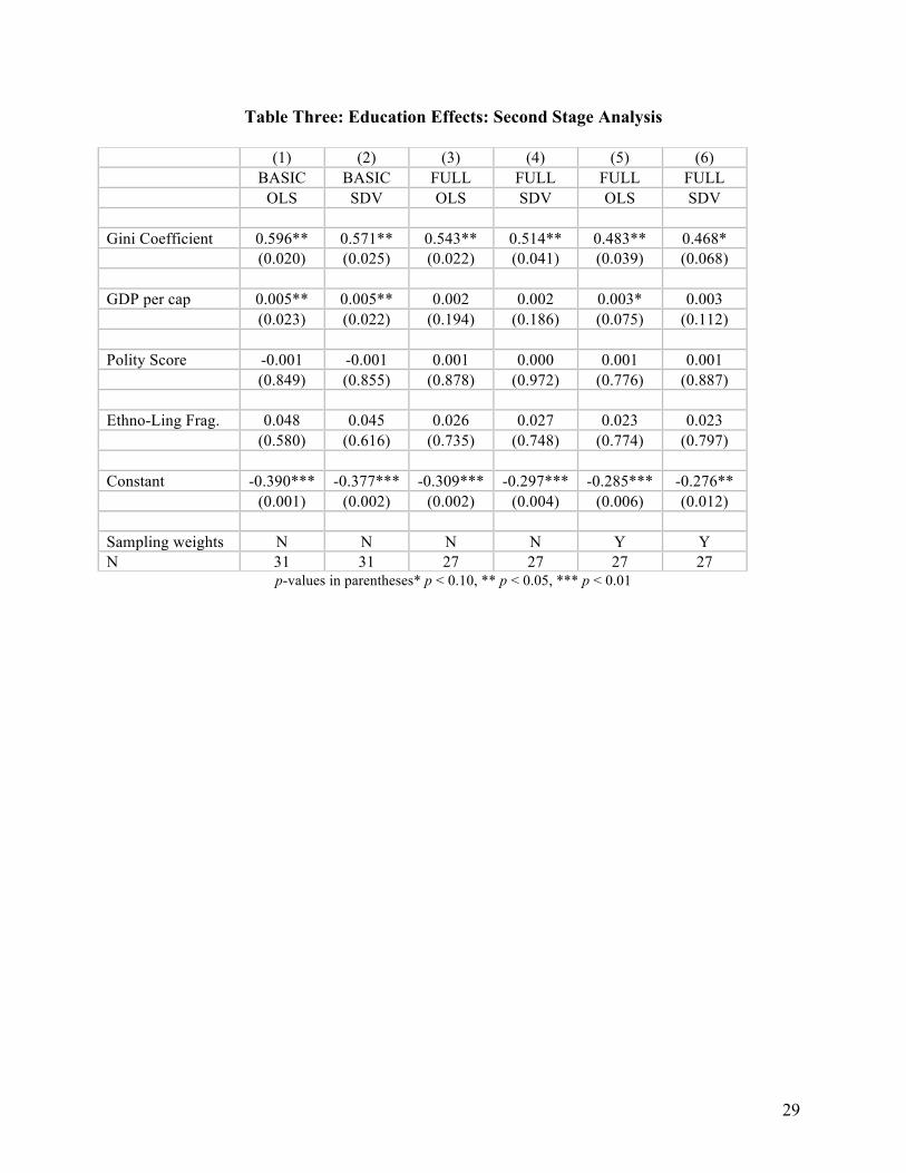
We now replace individual income in the 1st-stage regression with education, to see if the
results change any when we use this proxy variable. Table Three performs the same analysis as
in Table Two. Models 1 and 2 are basic specifications with just education included as an
independent variable in the 1st stage. Here we see strong effects at the national level of both

19
income inequality and income per capita on the relationship between education and redistribution
preferences. These results mimic those shown in Table Two, in that the positive effect means
that the estimated effect of education on preferences for redistribution moves from negative to
positive as cross-national inequality increases. This effect persists when we move to the full
specifications in Models 3 through 6, although the estimated effect for GDP per capita declines.
Figures Two (a) and Two (b) demonstrate the relationship between national income
inequality and the estimated effects of education on redistributive preferences. Again we see that
for below median inequality countries the estimated effects are negative (albeit less so in Figure
Two (b)), whereas they are spread around zero for higher levels of income inequality.
Accordingly, even if one thinks that educational status is a better proxy for long-run income than
transitory reported income in a sample, there remains no supportive evidence for Hypothesis 3;
indeed, the converse appears to be true.
3.4 ‘Typical’ Redistributive Preferences and the National Level of Inequality
We now examine the effect of inequality on average preferences for redistribution across
countries. This directly tests Hypothesis 2 – that the median voter is more support of
redistribution in high-inequality countries. The extension of the Meltzer-Richard framework to
democratization focuses on the preferences of the would-be median voter under autocracy–
typically operationalized as the person with median income. By comparing that person’s
preferences over redistribution in countries with different levels of inequality (and controlling for
national income) we gain insight on median “voter” preferences at different ratios of median to
mean income. Since redistributivist models use this ratio as their core exogenous variable, we
can directly examine their underlying mechanism. For purposes of comparison, we examine the

20
preferences of the median-income individual as well as the preferences of individuals at the 5th,
25th, 75th, and 95th percentiles of income, in order to see whether the redistributive preferences of
the poor and of the rich vary across different contexts of inequality.
How can we estimate the median voter’s preferences? To do so we estimate the constant
term for the first-stage regressions, re-specifying independent variables such that zero is a
meaningful quantity.9 We then regress these first-stage estimates on country-level characteristics
in a second stage regression. We do so five times, creating different estimates of the constant
term, by centering the individual income variable at the 5th, 25th, 50th, 75th, and 95th percentiles
respectively. We also mean-center all continuous independent variables in the first stage
regression, leaving dummy variables as they are.
Putting this together, this means that the constant term in each first-stage regression
reflects the expected support for redistribution for a citizen with mean religiosity, education,
number of children, and age, who is male and employed, and who has an income at either the 5th,
25th, 50th, 75th, or 95th percentile, depending on the model. The second stage regressions then
examine the effects of macro-level variables such as inequality on the preferences for
redistribution of this “typical” person at each of those percentiles. Hypothesis 2 asserts that the
median voter’s demand for redistribution should intensify as country-level inequality increases.
Furthermore, Hypothesis 3 implies that poorer citizens should also be even more pro-
redistribution in high inequality countries, and richer citizens should be even less pro-
redistribution in high inequality countries.
9 As noted above, to obtain estimates of the constant term for each country-year we must replace the ordered logit specification with a linear one – thus what we gain in insight here may be compromised somewhat by a potentially inappropriate specification. For the most part first-stage country-year linear regressions produce coefficients with similar substantive magnitude and statistical significance to the first-stage ordered logit specification, so in practice this does not appear to be a crucial distinction.

21
Tables Four (a) and (b) show OLS and SDV 2nd-stage regressions on the constant term at
different levels of respondent income. The core patterns are similar across both: Income
inequality is not related positively to the constant term in any of the models, contrary to the
expectations of both Hypotheses 2 and 3. Moreover, in the models for the 5th, 25th, and median
income citizen there is a negative relationship between income inequality and preferences for
redistribution. The Meltzer-Richard model expects a positive coefficient—as inequality
increases, demand for redistribution by the poor should also increase. Our results thus
completely reverse the redistributivist expectation—what we see is that poorer citizens in
relatively equal countries demand redistribution, but this preference weakens as national-level
inequality increases.
Hypothesis 3 also implies that opposition to redistribution among wealthy citizens will
intensify as country-level inequality increases. However, what we find is that as individual-level
incomes rise the coefficient on national income inequality becomes ever smaller in magnitude,
eventually becoming statistically insignificant. This means that among richer citizens, there is no
connection between national-level inequality and their “typical” redistribution preferences,
whereas among poorer citizens--including the median “voter,” rising inequality reduces support
for redistribution. Figure 3 shows estimates for all five of the income levels and makes clear the
gradual weakening of any relationship between inequality and redistributive preferences as
income rises. From both the perspective of the Meltzer-Richard model and the redistributivist
approach to democratization, all of these results are puzzling--to say the least.
4. In Conclusion: Interpreting our Results

22
So what does explain our results? When examining a set of autocratic countries, why, in
cross-national perspective, do preferences against redistribution increase with income only in
fairly equal countries? Our results provide no support for the Meltzer-Richard model or
redistributivist models of democratization. They are less troubling for own model of
democratization (Ansell and Samuels, 2010a), which presumes that different sets of economic
elites might hold substantially different preferences over taxation and redistribution. But, our
results do not directly corroborate our approach. In this concluding section, we explore some
possible explanations.
Our findings raise the question of why low-inequality countries appear to have more
strongly pro-redistributive poor citizens. A quick scan of Figures One through Three shows that
many, though far from all, of these states had Communist governments through much of the
postwar era. Conversely, many of the high-inequality states fit into the classic model of a
‘predatory state’. We argued that testing theories of individual redistributive preference
formation in autocracies avoids some of the endogeneity problems associated with doing so in
democracies where potential feedback effects from existing redistribution muddy the connection
between pre-fisc inequality and views about redistribution. While redistributive public spending
is generally lower in autocracies (at least cross-sectionally) much redistribution certainly took
place in Communist countries. Accordingly, such countries may produce feedback effects
whereby preexisting redistributive policies generates support among the poor for further
redistribution.
Tables Five (a) and Five (b) examine this contention by (a) controlling for past
Communist status or (b) excluding former Communist countries, and running 2nd-stage
regressions for the coefficients on income and education and for the constant term, centering

23
income at the 5th, 50th, and 95th percentiles.10 Doing so has a strong impact on the estimated
effects of inequality on these quantities of interest. In only Model 1 of Table Five (b) is the
coefficient significant at the ten percent level. However, there is no evidence in either of these
tables that Hypotheses 2 or 3 find any more support--even “controlling for communism,” we find
no support for the Meltzer-Richard model. We suggest that communist states acted rationally to
deliberately endogenize equality, in order to consolidate their political authority by quelling the
demands of rising economic groups that might challenge the political elite’s control of the
regime (as in Ansell and Samuels, 2010a). Creating support from the poor for the existence of
high levels of public spending might be a key tactic of autocratic regime consolidation.
A different explanation derives from Moene and Wallerstein (2001, 2003): individuals
may think of public pensions, unemployment compensation and health care as insurance
programs rather than redistributive policies. To the extent that citizens see government programs
as “risk-pooling” and believe that they are likely to benefit from those programs, rather than as
“downward” redistribution to people very much unlike them, a different relationship between
inequality and demand for government intervention in the market may arise More specifically,
since economists commonly assume that demand for insurance rises with income, the higher the
inequality, the less the median voter will favor these sorts of programs, and the more the wealthy
will favor them. The tricky thing here is to ascertain whether insurance programs are likely to
emerge in the kinds of countries under our analysis. While many social welfare programs in
developing post-authoritarian countries do bias towards wealthier citizens (Haggard and
Kaufman, 2008) it is not obvious that this effect is powerful enough to actually flip the poor’s
preferences to being anti-redistribution. Still, if public spending is targeted towards wealthier
10 We code Bosnia-Herzegovina, Croatia, Russia, China, Kyrgystan, and Vietnam as having Communist legacies.

24
citizens this provides further intuition as to why the rich are more ambivalent in high inequality
countries, where insurance style programs are more favorable toward them.
The empirical results presented in this paper cast considerable doubt on the value of the
median-voter assumption that underlies redistributivist models of democratization. Quite simply,
there is no micro-level evidence that as cross-national inequality increases in autocratic societies,
relatively poor voters will increasingly demand redistribution. Our next step is to detail how the
results here support our contractarian alternative approach.
References
Acemoglu, Daron and James Robinson. 2006. Economic Origins of Dictatorship and
Democracy. New York: Cambridge University Press.
Alesina, Alberto et al. 2003. “Fractionalization.” NBER Working Paper No. 9411. Available at
http://www.nber.org/papers/w9411, August 18, 2011.
Ansell, Ben and David Samuels. 2010a. “Inequality and Democratization: A Contractarian
Approach.” Comparative Political Studies.
Ansell, Ben and David Samuels. 2010b. “Democracy and Redistribution, 1880-1930:
Reassessing the Evidence.” Prepared for the 2010 Meeting of the American Political
Science Association, Washington DC.
Bartels, Larry. 2008. Unequal Democracy: The Political Economy of the New Gilded Age. New
York: Russell Sage Foundation.
Boix, Carles. 2003. Democracy and Redistribution. New York: Cambridge University Press.
Borjas, G.J., Sueyoshi, G.T., 1994. A two-stage estimator for probit models with structural group
effects. Journal of Econometrics 64, 165-182.

25
Epstein, David et al 2006. “Democratic Transitions.” American Journal of Political Science
50(3): 551-569.
Finseraas, Henning. 2009. “Income Inequality and Demand for Redistribution: A Multilevel
Analysis of European Public Opinion.” Scandinavian Political Studies 32(1): 94-119.
Haggard, Stefan and Robert Kaufman, 2008, Development, Democracy, and Welfare, Princeton
University Press, Princeton, NJ.
Huber, John and Piero Stanig. 2009. “Individual income and voting for redistribution across
democracies.” Unpublished. Columbia University.
Huber, John et al. 2005. “Institutional Context, Cognitive Resources and Party Attachments
Across Democracies.” Political Analysis 13 (4): 365-386.
Iversen, Torben and David Soskice, 2006. “Electoral Institutions and the Politics of Coalitions:
Why Some Democracies Redistribute More than Others.” American Political Science
Review 100(2): 165-181.
Jusko, Karen L. and W. Phillips Shively. 2005. “Applying a Two-Step Strategy to the Analysis
of Cross-National Public Opinion Data.” Political Analysis 13 (4): 327-344.
Kenworthy, Lane and Leslie McCall. 2007. “Inequality, Public Opinion and Redistribution.”
Socio-Economic Review 6:35-68.
Leoni, Eduardo. 2008. “Analyzing Multiple Surveys: Results from Monte Carlo Experiments.”
Unpublished manuscript, Columbia University.
Lewis, Jeffrey B. and Drew A. Linzer. 2005. “Estimating Regression Models in Which the
Dependent Variable Is Based on Estimates.” Political Analysis 13 (4): 345-364.
Lindert, Peter. 2004. Growing Public: Social Spending and Economic Growth Since the 18th
Century. New York: Cambridge University Press.

26
Lübker, Malte. 2007. “Inequality and the demand for redistribution: are the assumptions of the
new growth theory valid?” Socio-Economic Review 5(1): 117-148.
Marshall and Jaggers 2010. “Polity IV Project: Political Regime Characteristics and Transitions,
1800-2010. Dataset downloaded from http://www.systemicpeace.org/polity/polity4.htm,
August 20, 2011.
Meltzer, Alan and Scott Richard. 1981. “A Rational Theory of the Size of Government.” Journal
of Political Economy 89(5): 914-27.
Moene, Karl and Michael Wallerstein. 2001. “Inequality, Social Insurance and Redistribution.”
American Political Science Review 95: 859-874.
Moene, Karl. and Michael Wallerstein. 2003. “Earnings inequality and welfare spending: a
Disaggregated Analysis.” World Politics 55(4): 485-516.
Przeworski, Adam. 2010. Democracy and the Limits of Self-Government. New York: Cambridge
University Press.
Roemer, John. 2001. Political Competition. Cambridge: Harvard University Press.
Scheve, Kenneth and David Stasavage. 2006. “Religion and Preferences for Social Insurance.”
Quarterly Journal of Political Science 1(3): 255-286.
Shayo, Moses. 2009. “A Model of Social Identity with an Application to Political Economy:
Nation, Class, and Redistribution.” American Political Science Review 103(2): 147-174.

27
Table One: World Values Surveys - Autocracies Eligible for Inclusion in Analysis
Qualifying Countries Polity Score
Survey Year
Used in Table 2, Models 1 and 2
Used in Table 2, Models 3-6
Bosnia and Herzegovina -10 1998 Yes Yes Bosnia and Herzegovina -10 2001 Yes Yes
Burkina Faso 0 2007 Yes Yes China -7 1990 China -7 1995 China -7 2001 China -7 2007 Yes Yes
Croatia -5 1996 Yes Egypt -6 2000 Yes Yes Egypt -3 2008 Yes Yes
Ethiopia 1 2007 Yes Yes Hungary -7 1982
Iran 3 2000 Yes Yes Iran -6 2007 Yes Yes Iraq -10 2004 Iraq -10 2006
Jordan -2 2001 Yes Yes Jordan -3 2007
Kyrgyzstan -3 2003 Yes Yes Malaysia 3 2006 Yes Morocco -6 2001 Yes Yes Morocco -6 2007 Yes Nigeria -5 1990 Yes Yes Nigeria -6 1995 Yes Yes Nigeria 4 2000 Yes Yes Pakistan -6 2001 Yes Yes
Peru 1 1996 Yes Yes Russian Federation 0 1990 Yes Yes Russian Federation 3 1995 Yes
Rwanda -3 2007 Yes Yes Saudi Arabia -10 2003
Serbia and Montenegro -7 1996 Singapore -2 2002 Yes Yes
South Africa 4 1982 South Africa 5 1990 South Korea -5 1982
Tanzania -1 2001 Yes Yes Thailand -1 2007 Yes Yes Uganda -4 2001 Yes Yes Vietnam -7 2001 Yes Yes Vietnam -7 2006 Yes Yes Zambia 5 2007 Yes Yes
Zimbabwe -4 2001 Yes Yes

28
Table Two: Income Effects - Second Stage Analysis
(1) (2) (3) (4) (5) (6) BASIC BASIC FULL FULL FULL FULL OLS SDV OLS SDV OLS SDV Gini Coefficient 0.484 0.475 0.417* 0.408** 0.461** 0.442** (0.100) (0.103) (0.056) (0.048) (0.042) (0.038) GDP per cap 0.003* 0.003* 0.002 0.002 0.001 0.001 (0.057) (0.050) (0.150) (0.133) (0.301) (0.285) Polity Score 0.001 0.001 0.001 0.001 0.001 0.001 (0.855) (0.863) (0.724) (0.765) (0.853) (0.871) Ethno-Ling Frag. 0.054 0.051 0.037 0.028 0.048 0.035 (0.408) (0.431) (0.504) (0.603) (0.398) (0.513) Constant -0.312** -0.307** -0.244** -0.234** -0.265*** -0.250*** (0.014) (0.014) (0.014) (0.013) (0.010) (0.009) Sampling weights N N N N Y Y Observations 31 31 27 27 27 27
p-values in parentheses * p < 0.10, ** p < 0.05, *** p < 0.01
29
Table Three: Education Effects: Second Stage Analysis
(1) (2) (3) (4) (5) (6) BASIC BASIC FULL FULL FULL FULL OLS SDV OLS SDV OLS SDV Gini Coefficient 0.596** 0.571** 0.543** 0.514** 0.483** 0.468* (0.020) (0.025) (0.022) (0.041) (0.039) (0.068) GDP per cap 0.005** 0.005** 0.002 0.002 0.003* 0.003 (0.023) (0.022) (0.194) (0.186) (0.075) (0.112) Polity Score -0.001 -0.001 0.001 0.000 0.001 0.001 (0.849) (0.855) (0.878) (0.972) (0.776) (0.887) Ethno-Ling Frag. 0.048 0.045 0.026 0.027 0.023 0.023 (0.580) (0.616) (0.735) (0.748) (0.774) (0.797) Constant -0.390*** -0.377*** -0.309*** -0.297*** -0.285*** -0.276** (0.001) (0.002) (0.002) (0.004) (0.006) (0.012) Sampling weights N N N N Y Y N 31 31 27 27 27 27
p-values in parentheses* p < 0.10, ** p < 0.05, *** p < 0.01

30
Table Four (a): Constant Term Analysis: OLS Second Stage Regression
(1) (2) (3) (4) (5)
5th percentile 25th percentile Median 75th percentile 95th
percentile Gini Coefficient -7.053* -6.516* -5.999* -5.075 -3.920 (0.087) (0.087) (0.089) (0.105) (0.126) GDP per cap -0.006 -0.003 -0.001 -0.000 -0.004 (0.749) (0.865) (0.922) (0.986) (0.747) Polity Score -0.023 -0.020 -0.029 -0.032 -0.030 (0.687) (0.690) (0.544) (0.471) (0.460) Ethno-Ling Frag. 1.017 1.115 1.262 1.333 1.434* (0.364) (0.271) (0.191) (0.132) (0.067) Constant 6.912*** 6.513*** 6.117*** 5.586*** 4.920*** (0.002) (0.002) (0.002) (0.001) (0.001) Observations 26 26 26 26 26
p-values in parentheses * p < 0.10, ** p < 0.05, *** p < 0.01
Table Four (b): Constant Term Analysis: SDV Second Stage Regression
(1) (2) (3) (4) (5) 5th 25th Median 75th 95th Gini Coefficient -6.972* -6.450* -5.960* -5.016 -3.808 (0.092) (0.092) (0.094) (0.112) (0.149) GDP per cap -0.005 -0.003 -0.001 0.000 -0.003 (0.758) (0.876) (0.941) (0.992) (0.787) Polity Score -0.025 -0.021 -0.030 -0.033 -0.031 (0.657) (0.669) (0.531) (0.460) (0.450) Ethno-Ling Frag. 1.095 1.166 1.310 1.385 1.498* (0.328) (0.252) (0.177) (0.119) (0.059) Constant 6.828*** 6.454*** 6.070*** 5.529*** 4.834*** (0.003) (0.002) (0.002) (0.002) (0.001) Observations 26 26 26 26 26
p-values in parentheses * p < 0.10, ** p < 0.05, *** p < 0.01

31
Table Five (a) – Communism as a Control
(1) (2) (3) (4) (5) Income Education Constant 5th Constant 50th Constant 95th Gini Coefficient 0.499 0.291 -6.316 -5.328 -3.144 (0.129) (0.241) (0.187) (0.188) (0.248) GDP per cap 0.001 0.002* -0.002 0.002 0.000 (0.346) (0.053) (0.932) (0.904) (0.994) Polity Score 0.001 -0.002 -0.003 -0.011 -0.010 (0.744) (0.654) (0.970) (0.840) (0.823) Ethno-Ling Frag. 0.038 0.010 1.132 1.370 1.536** (0.550) (0.859) (0.271) (0.128) (0.035) Communism 0.024 -0.085* 0.467 0.401 0.448 (0.688) (0.088) (0.583) (0.570) (0.365) Constant -0.278* -0.189* 6.510*** 5.750*** 4.515*** (0.078) (0.060) (0.008) (0.006) (0.001) Observations 27 27 26 26 26
Table Five (b) – Non-Communist Countries Only
(1) (2) (3) (4) (5) Income Education Constant 5th Constant 50th Constant 95th Gini Coefficient 0.672* 0.298 -9.217 -7.885 -5.192 (0.092) (0.385) (0.119) (0.128) (0.165) GDP per cap 0.001 0.003* 0.008 0.012 0.010 (0.512) (0.064) (0.736) (0.559) (0.533) Polity Score 0.002 -0.005 -0.016 -0.023 -0.023 (0.783) (0.393) (0.850) (0.738) (0.662) Ethno-Ling Frag. 0.009 0.018 1.910 2.041* 2.111** (0.913) (0.802) (0.156) (0.089) (0.032) Constant -0.330* -0.201 7.188*** 6.351*** 4.960*** (0.058) (0.114) (0.006) (0.005) (0.003) Observations 20 20 20 20 20
p-values in parentheses * p < 0.10, ** p < 0.05, *** p < 0.01

32
Figure One (a): Basic Income Effect
Figure One (b): Full Specification Income Effect

33
Figure Two (a): Basic Effect of Education
Figure Two (b): Full Specification Effect of Education

34
Figure Three: Estimates of Support for Redistribution for ‘Typical’ Citizens at
Varying Levels of Income, against Income Inequality
Note: All figures show estimate of constant term from linear regressions of preferences over redistribution at the country-year level for male, employed citizens with mean education, religiosity, children, and age. The dashed line represents a constant term of five, to help compare scatterplots.