SOEPpaperson Multidisciplinary Panel Data Research

Inequality-adjusted gender wage differentials in Germany

Ekaterina Selezneva and Philippe Van Kerm

579 201

3SOEP — The German Socio-Economic Panel Study at DIW Berlin 579-2013

SOEPpapers on Multidisciplinary Panel Data Research at DIW Berlin This series presents research findings based either directly on data from the German Socio-Economic Panel Study (SOEP) or using SOEP data as part of an internationally comparable data set (e.g. CNEF, ECHP, LIS, LWS, CHER/PACO). SOEP is a truly multidisciplinary household panel study covering a wide range of social and behavioral sciences: economics, sociology, psychology, survey methodology, econometrics and applied statistics, educational science, political science, public health, behavioral genetics, demography, geography, and sport science. The decision to publish a submission in SOEPpapers is made by a board of editors chosen by the DIW Berlin to represent the wide range of disciplines covered by SOEP. There is no external referee process and papers are either accepted or rejected without revision. Papers appear in this series as works in progress and may also appear elsewhere. They often represent preliminary studies and are circulated to encourage discussion. Citation of such a paper should account for its provisional character. A revised version may be requested from the author directly. Any opinions expressed in this series are those of the author(s) and not those of DIW Berlin. Research disseminated by DIW Berlin may include views on public policy issues, but the institute itself takes no institutional policy positions. The SOEPpapers are available at http://www.diw.de/soeppapers Editors: Jürgen Schupp (Sociology) Gert G. Wagner (Social Sciences, Vice Dean DIW Graduate Center) Conchita D’Ambrosio (Public Economics) Denis Gerstorf (Psychology, DIW Research Director) Elke Holst (Gender Studies, DIW Research Director) Frauke Kreuter (Survey Methodology, DIW Research Professor) Martin Kroh (Political Science and Survey Methodology) Frieder R. Lang (Psychology, DIW Research Professor) Henning Lohmann (Sociology, DIW Research Professor) Jörg-Peter Schräpler (Survey Methodology, DIW Research Professor) Thomas Siedler (Empirical Economics) C. Katharina Spieß (Empirical Economics and Educational Science)

ISSN: 1864-6689 (online)

German Socio-Economic Panel Study (SOEP) DIW Berlin Mohrenstrasse 58 10117 Berlin, Germany Contact: Uta Rahmann | soeppapers@diw.de

Inequality-adjusted gender wage differentialsin Germany∗

Ekaterina SeleznevaInstitut for East and Southeast European Studies, Regensburg, Germany

Philippe Van KermCEPS/INSTEAD, Luxembourg

August 2013

Abstract

This paper exploits data from the German Socio-Economic Panel (SOEP)to re-examine the gender wage gap in Germany on the basis of inequality-adjusted measures of wage differentials which fully account for gender differ-ences in pay distributions. The inequality-adjusted gender pay gap measuresare significantly larger than suggested by standard indicators, especially inEast Germany. Women appear penalized twice, with both lower mean wagesand greater wage inequality. A hypothetical risky investment question col-lected in 2004 in the SOEP is used to estimate individual risk aversion pa-rameters and benchmark the ranges of inequality-adjusted wage differentialsmeasures.

Keywords: gender gap; wage differentials; wage inequality; expected utility;risk aversion; East and West Germany; SOEP ; Singh-Maddala distribution ;copula-based selection model

JEL classification codes: D63 ; J31 ; J70

∗This paper was prepared when Van Kerm visited the Institute for East and Southeast European Studies (IOSRegensburg) whose support and hospitality are gratefully acknowledged. The project was also supported by corefunding for CEPS/INSTEAD from the Ministry of Higher Education and Research of Luxembourg. The dataused in this publication were made available to us by the German Socio-Economic Panel Study (SOEP) at theGerman Institute for Economic Research (DIW Berlin). We thank Richard Frensch, Jürgen Jerger and DonaldWilliams for stimulating comments and discussion. Comments from participants to the 2011 New Directionsin Welfare congress (OECD Paris), the 2012 biennial EACES conference (Perth) and the 5th ECINEQ meeting(Bari) are gratefully acknowledged.

1 Introduction

The gender gap in pay in Germany is often considered as one of the largest in Europe. Ac-

cording to recent IAB InfoPlattform briefing, the average gross hourly earnings of women is

22 percent lower than men, for an EU average of 16 percent.1 Eurostat’s 2011 estimate of Ger-

many’s (unadjusted) gender pay gap is third only to Estonia and Austria among 26 european

countries.2

Factors contributing to the gap are generally sought in career breaks, part-time employment

and relative concentration of women in low skill and low pay occupations (Al-Farhan, 2010a,

Antonczyk et al., 2010, Heinze, 2010). The size of the gender gap is known to differ markedly

in Western and Eastern Germany: while mean wages are generally lower in Easter Germany,

women face a much smaller penalty relative to men than in Western Germany (see, e.g., Hunt,

2002, Smolny and Kirbach, 2011, Kohn and Antonczyk, 2013). Smolny and Kirbach (2011)

observe that the gender wage gap is one of the few statistics for which there is no convergence

to Western levels in the period 1990–2008.

At the same time, Germany recently experienced an increase in overall wage inequality;

see, e.g., Dustmann et al. (2009), Fuchs-Schündeln et al. (2010), Card et al. (2013). Accord-

ing to Al-Farhan’s (2010b) analysis of the German Socio-Economic Panel (SOEP) data, the

wage distribution in Germany appeared to stabilize at historically high levels of inequality in

the recent ten years, while Antonczyk et al. (2010, 2011) still find increasing wage inequality

between 2001 and 2006 using Structure of Earnings data. Observing high levels of wage in-

equality with a large gender gap in pay is consistent with the demonstration by Blau and Kahn

(1992, 1996, 1997) that wage inequality is positively associated to the gender pay gap. Al-

Farhan (2010a) shows indeed that recent trends in the gender pay gap and in wage inequality

in Germany are driven by common underlying factors such as changes in potential experience,

in workers occupational positions and in firm sizes.

In this context of a high gender pay gap and historically high levels of wage inequality,

1See http://infosys.iab.de/infoplattform/dokSelect.asp?pkyDokSelect=71 (ac-cessed August 6, 2013).

2See http://epp.eurostat.ec.europa.eu/statistics_explained/index.php/Gender_pay_gap_statistics (accessed August 6, 2013).

1

we undertake a re-examination of the German gender gap using inequality-adjusted measures

of wage differentials. A standard measure of the gender gap gives (one minus) “the cents a

woman makes on average for every dollar an observationally equivalent man makes on av-

erage.” Unlike the raw figures mentioned in the opening sentences of this paper, such an

indicator controls for gender differences in human capital (and possibly job characteristics)

and compares observationally equivalent men and women. However it remains somewhat lim-

ited in that it focuses on comparisons of mean wages of men and women. It has long been

recognised that a comprehensive assessement of wage differentials should consider the whole

wage distributions of men and women –not just the mean– and comparisons be made on the

basis of utility functionals defined over such distributions (see,e.g., Dolton and Makepeace,

1985). This is particularly relevant in a context of rising wage inequality if trends in wage

dispersion vary by gender.

Using SOEP data on a subsample of individuals aged 25–55 over the period 1999–2008,

we estimate upper and lower bounds for indices of wage differentials that incorporate a dis-

tributional dimension as proposed in Van Kerm (2013). The range includes a standard wage

differential index focused on mean wages as special case. We find that this special case is

(close to) the lower bound and that ignoring distributional concerns potentially underestimates

the magnitude of the wage gap by up to three-fold in Eastern Germany and up to fifty percent

in Western Germany. The much larger impact of accounting for inequality in Eastern Germany

challenges current evidence that the gender gap is smaller in the East: taking male-female in-

equality differences into account very much reduces the contrast between Eastern and Western

Germany.

We estimate the measures with and without correction for endogenous labour market par-

ticipation using a copula-based selection model (Smith, 2003) and provide lower and upper

bounds for the inequality-adjusted gender wage gap over a broad range of inequality aversion

parameters. Additionally, we take advantage of a special module on risk attitudes collected

in the 2004 wave of the survey (Dohmen et al., 2005, 2011) to estimate individual-level co-

efficients of relative risk aversion which, when plugged in the inequality-adjusted wage gap

measure provide benchmark indicators relying on individual-specific risk aversion parameters.

These benchmarks turn out to be close to the upper bounds in our range of inequality-adjusted

indicators.

2

The paper proceeds as follows. Section 2 describes the inequality-adjusted measure of

wage differentials and estimation methods. Section 3 provides information on the sample and

variables of interest and describes construction of the individual measures of risk aversion

from answers to the SOEP hypothetical risky investment question. Results are presented in

Section 4. Section 5 concludes.

2 Inequality-adjusted measures of wage differentials

As mentioned in the Introduction, a standard indicator of the wage gap gives the “cents a

woman makes on average for every dollar an observationally equivalent man makes on aver-

age” (see, e.g., Jenkins, 1994):

∆1 = exp

[∫Ξ

[log(µwx)− log

(µmx) ]

hw(x)dx

](1)

where (i) µwx is the average wage of a woman with characteristics x (e.g., education, experi-

ence, etc.) and µmx is the average wage of a man with the same characteristics x and (ii) hw(x)

is the (multivariate) probability density function of characteristics x among women. ∆1 is

usually estimated from wage regressions of the form

log(wi) = xiβs + ui, i = 1, . . . , N s (2)

for s ∈ {m,w}, and then pluging regression coefficients to obtain

∆OB1 = exp

[∫Ξ

x (βw − βm)hw(x)dx

]θ (3)

= exp

[xw (βw − βm)

]θ (4)

where xw is the vector of average women characteristics.3 ∆OB1 is the ubiquitous Oaxaca-

Blinder measure of ‘unexplained’ wage differences (see, e.g., Fortin et al., 2011).4

The anatomy of (1) reveals a double averaging: first by considering the differences in av-

erage wage of men and women (conditionally on characteristics x) and, second, by averaging

3θ reflects differences in residual variance in the wage regressions for men and women (see Blackburn, 2007,Van Kerm, 2013).

4Women are taken as group of interest and men as reference group. The measure captures the disadvantage ofwomen relative to men, what Jenkins (1994) calls ‘discrimination against women’. Other choices are obviouslyavailable: as Fortin et al. (2011) argue, this question does not have any unambiguous econometric solution.

3

these differences over the characteristics of women. This approach, albeit empirically conve-

nient, has been criticized for putting narrow focus on mean differences and discarding norma-

tively relevant and empirically important distributional differences (Dolton and Makepeace,

1985, Jenkins, 1994, del Río et al., 2011). To address this concern, Van Kerm (2013) proposes

an inequality-adjusted measure of wage differentials that is a straightforward extension of (1):

∆2(ε) = exp

[∫Ξ

[log(C(Fw

x ; ε))− log

(C(Fm

x ; ε))]hw(x)dx

](5)

where C(F sx ; ε) denotes a (conditional) power mean of order (1 − ε). The normative sig-

nificance of ∆2(ε) stems from the fact that C(F sx ; ε) is also the certainty-equivalent for the

uncertain outcome described by the distribution F sx and constant relative risk aversion von

Neumann-Morgenstern expected utility over the wage distribution:

C(F ; ε) =

(∫ ∞0

y1−εdF (y)

) 11−ε

for ε 6= 1 and C(F ; 1) = exp[∫∞

0ln(y)dF (y)

].

∆2(ε) is a simple extension of ∆1. Both measures are equal for ε = 0. Adopting ε > 0

leads to C(F ; ε) ≤ C(F ; 0): dispersion in the wage distribution is penalized. Adopting ε < 0

leads to C(F ; ε) ≥ C(F ; 0): dispersion in the wage distribution is rewarded. This simple

framework makes it straightforward to incorporate inequality adjustments in the gender wage

gap assessment. When women with characteristics x face wage distributions with greater in-

equality than observationally equivalent men, this will inflate the wage gap index for any index

with positive ε. On the contrary, lower inequality among women distributions may compen-

sate for lower wages and thereby mitigate standard estimates of the wage gap. By similar ar-

guments, assuming that greater inequality should be positively rewarded and computing wage

gap measures with negative ε (that is, assuming preference for risk or inequality) higher in-

equality may mitigate (or worsen) the gender wage gap if there is more (or less) inequality in

the wage distributions of women than of observationally equivalent men.

Note that inequality comparisons between men and women are made on conditional wage

distributions Fwx and Fm

x . A related branch of the literature focuses on comparisons of quan-

tiles of the unconditional wage distributions of men and women; see, among others, Juhn et al.

(1993), Machado and Mata (2005), Melly (2005), Firpo et al. (2009) on methods and Anton-

czyk et al. (2010), Heinze (2010) or Al-Farhan (2010a) for recent applications to the gender

wage gap in Germany. This approach also departs from a narrow focus on mean wages and, by

4

comparing quantiles of the wage distributions, flexibly identifies differences in pay at, say, the

bottom or the top of the wage distributions (e.g., to identify ‘glass ceiling’ effects). The focus

is however on understanding and decomposing differences in the unconditional wage distribu-

tion of men and women (disentangling composition effects from wage structure effects).5 Our

aim instead is to assess the impact and relevance of introducing normative considerations of

inequality in aggregate assessments of the gender wage gap and we base this on comparisons

of conditional wage distributions.

Equation (5) defines a class of wage gap measures indexed by the parameter of inequal-

ity aversion. We will report estimates for ε in the range [−4, 10] covering a broad range of

positions over inequality aversion (ε > 0) or preference (ε < 0). Variations in the statistic

for different ε will inform us of the degree to which overall (conditional) wage distributions

differ between women and observationally equivalent men in our sample. We will interpret

the maximum and minimum values for ∆2(ε) in this range as upper and lower bounds for the

inequality-adjusted gender wage gap.

In principle, a distinct ε could also be specified for each women in the sample, or for each

configuration of characteristics to reflect heterogeneity in individual-level attitudes towards

inequality or risk. The SOEP dataset contains individual-level measures of risk attitudes in

a special module in the 2004 wave of the survey. Responses to the small set of questions

asked were validated in an incentive compatible field experiment with representative subjects

(Dohmen et al., 2011). To benchmark our estimation results with constant ε for all women, we

will exploit individual-level parameter estimates of risk aversion that can be derived from this

module under the assumption of constant relative risk aversion utilities. Under the assumption

that risk aversion parameters so derived can also reflect individual positions regarding wage

inequality, we will estimate ∆2(εi) with heterogenous, individual-level εi parameters. This

index will benchmark the estimated bounds for the wage gap. The degree to which the gap

estimate will differ from indices with constant parameters will depend both on the size of

the estimated risk-aversion parameters and on the association between individual-level risk

aversion parameters and differences in wage inequality across gender.

5The unconditional wage distribution for women is Fw(y) =∫Fw

x (y)hw(x)dx and counterfactual uncon-ditional distribution that would be observed if women were paid as men is F ∗(y) =

∫Fm

x (y)hw(x)dx whichcan be inverted to consider unconditional quantiles; see, e.g., Albrecht et al. (2003), Millimet and Wang (2006),Arulampalam et al. (2007), Christofides et al. (2013) for applications to the gender wage gap.

5

Calculation of ∆2(ε) requires estimates of conditional wage distributions Fmx and Fw

x for

all x observed in the sample. Several alternative estimators can be chosen from, such as quan-

tile regression, non-parametric kernel estimation, ‘distribution regression’; see, e.g., Hall et al.

(1999) for non-parametric approaches or Rothe (2010) and Chernozhukov et al. (2012) for

recent general discussions. We follow Biewen and Jenkins (2005) and Van Kerm (2013) and

adopt a fully parametric approach. Wages are specified as Singh-Maddala distributed condi-

tionally on covariates, with the three parameters of the distribution allowed to vary log-linearly

with covariates:

F sx(y) = 1−

[1 +

(y

bs(x)

)as(x)]−qs(x)

(6)

where bs(x) = exp(xθsb) is a scale parameter, as(x) = exp(xθsa) is a shape parameter modify-

ing both tails and qs(x) = exp(xθsq) is a shape parameter modifying the upper tail (Singh and

Maddala, 1976). Power means for the Singh-Maddala distribution have convenient closed-

form expressions. This makes estimation of ∆2(ε) easy from coefficient estimates of model

(6):

C(F sx ; ε) = bs(x)

(Γ (1 + (1− ε)/as(x)) Γ (qs(x)− (1− ε)/as(x))

Γ (qs(x))

) 11−ε

(7)

where Γ(·) is the Gamma function and (θsa, θsb , θ

sq) are (say, maximum likelihood) estimates of

the Singh-Maddala parameters (Kleiber and Kotz, 2003). Such a specification, albeit paramet-

ric, is flexible and allows for broad variations in degrees of skewness and kurtosis of the wage

distributions. It can also deal with the heavy tail typical of earnings data.

A key advantage of the parametric approach over quantile regression or non-parametric

procedures is that it can be adapted to handle endogenous labour market participation.6 As is

well-known, endogenous selection may lead to an over-estimation of the wage distributions

when estimated only from observed wages. A differential effect of sample selection between

women and men might appear, as the former group is more likely to include workers with

lower earnings potential and/or higher reservation wages. See Hunt (2002) for a discussion of

this in the context of East Germany.

Van Kerm (2013) shows that a Singh-Maddala distribution for wages can be combined with

the standard Heckman-selection-type normality assumption (Heckman, 1979) to correct for

6See Huber and Melly (2011) on issues with quantile regression with sample selection.

6

endogenous participation using a copula-based selection model (Smith, 2003). Say z denotes

participation for a given agent with wage y observed if z = 1. Let z∗ be a latent propensity

to participate in the labour market with z = 1 if z∗ > 0 and z = 0 otherwise. Assuming

the pair (y, z∗) is jointly distributed with cumulative distribution Hx and expressing Hx using

its copula, the marginal Singh-Maddala distribution for y and an assumed distribution for the

latent z∗ (denoted Gx) leads to

Hs(y, z∗) = Ψsx(F sx(y), Gs

x(z∗)) (8)

As in standard selectivity-corrected regression models, Gsx can be assumed normal with mean

xδs and unit variance. Following Van Kerm (2013), we take Ψs to be a Clayton copula:

Ψ(u, v; θsC) =(u−θ

sC + v−θ

sC − 1

)−1/θsC (9)

where θsC is an association parameter to be estimated. Joint estimation of θsa, θsb , θ

sq , δ

s and

θsC , for example via maximum likelihood, leads to estimates of the Singh-Maddala distribution

appropriately corrected for endogenous labour market participation. See Christofides et al.

(2013) for a recent application of this model.

For inference on estimates of ∆2(ε), we assess sampling variability on the basis of boot-

strap resampling. We implement the repeated half-sample bootstrap algorithm of Saigo et al.

(2001) with a resampling that takes into account the repetition of individuals in the pooled

longitudinal dataset as well as the sampling dependence between observations implied by the

survey design (stratification and clustering).

3 Data

3.1 Sample definition and labour market variables

The German Socio-Economic Panel (SOEP) is a nationally representative longitudinal survey

on living conditions in Germany collected annually by the Deutsches Institut fur Wirtschafts-

forschung (DIW, Berlin). Multiple topics are covered and include, e.g., income and employ-

ment, housing, health, educational achievements (see Wagner et al., 1993, 2007). SOEP data

are available yearly since 1984 (since 1990 for East Germany). For our analysis we pool ten

waves of data covering the period 1999–2008.

7

To limit the influence on wages of transitions into and out of the labour market, we restrict

our analysis to respondents aged between 25 and 55. We consider the wages of individuals

working in the private or public sector at least 15 hours per week in a regular (full-time or part-

time) job. This excludes workers on vocational training, in sheltered workshops, or reporting

marginal or irregular part-time employment. Self-employed workers are excluded as their

wage rate is ill-defined. We exclude workers in the agricultural sector. Individuals with hourly

wage below e4 are considered as out of regular employment. Cross-section sample weights

are used throughout the analysis to correct for unequal sampling probabilities in the SOEP

sampling design.

Gross hourly wage in the main job is calculated as gross earnings received in the month

preceding interview divided by 4.32 and then by average weekly hours worked. Gross monthly

earnings exclude additional payments such as holiday money or back-pay, while include money

earned for overtime. Hours of work include information on average hours worked normally

during a week, including overtime. We inflate all wages to 2008 prices using the national

consumer price index.7 To prevent outlying data from driving our estimates, abnormally large

wages are excluded: observations with hourly wages above e70 are discarded. We also recode

as missing any hourly wage from a person reported as normally working more than 65 hours

per week.

Our final samples consist of 24,036 male observations and 17,371 female observations for

Western Germany (with mean real hourly wages of e17.01 and e13.35, respectively), and

of 7,060 male observations and 6,852 female observations for Eastern Germany (with mean

wages of e11.69 and e10.81 euros, respectively). Descriptive statistics on wages percentiles

and means by gender and region along with sample sizes are presented in Table 1. Note the

regional contrast in differences between men and women in both wages and labour market

participation.

The vector of individual characteristics we condition upon when computing our gender

gap index contains age (in quadratic form), educational attainment (recorded as five cate-

gories from general elementary (or less) to higher, post-secondary education), years of po-

tential labour market experience (computed as age minus years normally required to complete

7Data on CPI are taken from the website of the Germany Federal Statistical Office,http://www.destatis.de.

8

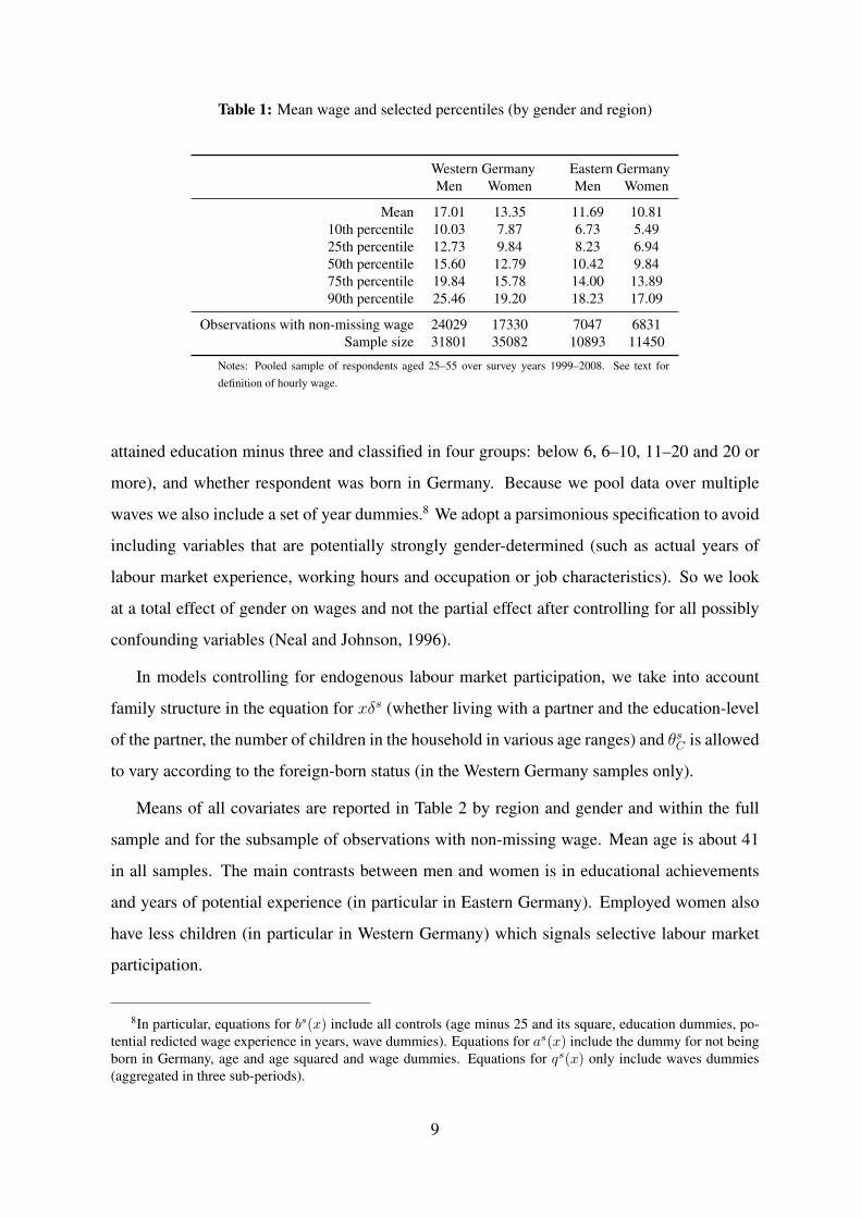
Table 1: Mean wage and selected percentiles (by gender and region)

Western Germany Eastern GermanyMen Women Men Women

Mean 17.01 13.35 11.69 10.8110th percentile 10.03 7.87 6.73 5.4925th percentile 12.73 9.84 8.23 6.9450th percentile 15.60 12.79 10.42 9.8475th percentile 19.84 15.78 14.00 13.8990th percentile 25.46 19.20 18.23 17.09

Observations with non-missing wage 24029 17330 7047 6831Sample size 31801 35082 10893 11450

Notes: Pooled sample of respondents aged 25–55 over survey years 1999–2008. See text fordefinition of hourly wage.

attained education minus three and classified in four groups: below 6, 6–10, 11–20 and 20 or

more), and whether respondent was born in Germany. Because we pool data over multiple

waves we also include a set of year dummies.8 We adopt a parsimonious specification to avoid

including variables that are potentially strongly gender-determined (such as actual years of

labour market experience, working hours and occupation or job characteristics). So we look

at a total effect of gender on wages and not the partial effect after controlling for all possibly

confounding variables (Neal and Johnson, 1996).

In models controlling for endogenous labour market participation, we take into account

family structure in the equation for xδs (whether living with a partner and the education-level

of the partner, the number of children in the household in various age ranges) and θsC is allowed

to vary according to the foreign-born status (in the Western Germany samples only).

Means of all covariates are reported in Table 2 by region and gender and within the full

sample and for the subsample of observations with non-missing wage. Mean age is about 41

in all samples. The main contrasts between men and women is in educational achievements

and years of potential experience (in particular in Eastern Germany). Employed women also

have less children (in particular in Western Germany) which signals selective labour market

participation.

8In particular, equations for bs(x) include all controls (age minus 25 and its square, education dummies, po-tential redicted wage experience in years, wave dummies). Equations for as(x) include the dummy for not beingborn in Germany, age and age squared and wage dummies. Equations for qs(x) only include waves dummies(aggregated in three sub-periods).

9

Table 2: Covariate means for observations with non-missing wage (1) and in the full sample (2) (bygender and region)

Western Germany Eastern GermanyMen Women Men Women

(1) (2) (1) (2) (1) (2) (1) (2)

Age 41.59 40.63 41.03 40.24 41.01 41.00 41.71 40.59Foreign born 0.17 0.18 0.16 0.19 0.01 0.01 0.00 0.02

Education:General Elementary 0.10 0.11 0.10 0.16 0.04 0.06 0.03 0.06

Middle Vocational 0.51 0.51 0.51 0.53 0.62 0.62 0.53 0.56Vocational Plus Abitur 0.07 0.08 0.13 0.09 0.06 0.04 0.05 0.04

Higher Vocational 0.10 0.10 0.06 0.08 0.10 0.11 0.11 0.07Higher Education 0.22 0.20 0.19 0.15 0.19 0.18 0.28 0.27

Potential experience:0–10 years 0.03 0.04 0.04 0.04 0.06 0.03 0.03 0.06

11–20 years 0.22 0.27 0.28 0.27 0.26 0.24 0.20 0.2621–30 years 0.36 0.35 0.32 0.34 0.31 0.36 0.36 0.33

31 years or more 0.34 0.31 0.33 0.31 0.32 0.31 0.36 0.31Education of partner:

No partner 0.30 0.31 0.41 0.29 0.37 0.35 0.28 0.28General Elementary 0.10 0.12 0.05 0.09 0.03 0.03 0.02 0.03

Middle Vocational 0.35 0.36 0.30 0.35 0.38 0.38 0.43 0.42Vocational Plus Abitur 0.08 0.06 0.05 0.04 0.03 0.02 0.03 0.02

Higher Vocational 0.05 0.06 0.07 0.08 0.05 0.04 0.10 0.09Higher Education 0.11 0.09 0.12 0.14 0.15 0.18 0.14 0.16

Number of children in age range:0–1 0.03 0.05 0.01 0.05 0.04 0.04 0.01 0.042–4 0.12 0.13 0.06 0.14 0.07 0.09 0.08 0.115–7 0.13 0.14 0.09 0.16 0.10 0.08 0.13 0.11

8–10 0.13 0.14 0.12 0.16 0.07 0.08 0.10 0.1011–12 0.10 0.10 0.08 0.10 0.05 0.07 0.04 0.0813–15 0.12 0.14 0.10 0.16 0.05 0.13 0.07 0.1616–18 0.09 0.10 0.09 0.12 0.08 0.13 0.09 0.16

Notes: Pooled sample of respondents aged 25–55 over survey years 1999–2008. See text fordefinition of variables.

10

3.2 Individual measures of risk aversion

The SOEP dataset contains individual-level measures of risk attitudes in a special module col-

lected in the 2004 wave of the survey. One particular question allows us to approximate an

individual-level risk aversion parameter εi under the assumption of CRRA utilities. Individual-

level parameters can then be used in (5) to compute a measure of wage differentials that incor-

porates heterogeneous individual-level attitudes towards risk, instead of a constant parameter.

After a range of questions on their personal willingness to take risks (in general and in a

number of specific contexts), survey respondents were presented an hypothetical investment

opportunity. They were asked to report how much of a windfall gain of e100,000 they would

be willing to invest in a risky asset. With equal probability, they would lose half of the value

of their investment or they would double their investment. Respondents were asked to select

a value for the amount invested k ∈ {e0,e20000,e40000,e60000,e80000,e100000}. The

expected gain after investment of an amount k in the lottery is G(k) = (100000− k) + 12(k

2+

2k) = 100000 + k4. We follow Dohmen et al. (2005, 2011) and combine each respondent’s

investment choice with measures of initial endowments taken from the data to infer values for

individual CRRA coefficients.

Under the assumed CRRA utility function, expected utility of respondent i with initial

wealth endowments w0i investing an amount k of the windfall e100000 gain (denoted W ) is

u(w0i , k; εi) =

1

2(1− εi)

((w0i +W − k

2

)1−εi+ (w0

i +W + 2k)1−εi

)(10)

where εi is the respondent’s CRRA. εi is unknown but we assume that the investment level ki

selected by the respondent leads to a higher expected utility than any other possible investment

k−i:

u(w0i , ki; εi) ≥ u(w0

i , k−i; εi). (11)

Plausible estimates of risk aversion coefficients for respondent i are given by the range of

values of εi for which inequality (11) is satisfied.9 Note that the ordinal nature of the set of

possible investment choices implies that we are only able to estimate ranges of coefficients of

risk aversion. We will therefore construct different values for (5) based on lower bounds and

9In our application, we solve this problem numerically on a grid of 21 potential values for εi ∈{0, 0.5, 1, . . . , 10}.

11

upper bounds for individual risk aversion coefficients. Note also that the range of investment

options does not allow us to capture any negative risk aversion: the lower bound for risk

aversion is set to 0. For plausibility, we also impose a maximum value for εi of 10.

Table 3 shows estimates of the individual measures of risk aversion obtained in our sample

with three alternative measures of initial endowments w0i : the net worth of household wealth

(total household assets minus debts), annual household disposable income, and neglect of

initial endowments altogether (w0i = 0).10 Using annual disposable income as a level of

initial endowments seems to lead to a more credible distribution of CRRA coefficients (which

mostly range within the limits of zero and 10) than using net worth. Using data on wealth as

endowment leads to more extreme estimates of risk aversion. Like us, Dohmen et al. (2005)

find estimated parameters of risk aversion up to 20 and suggest such extreme values to be

potentially explained by measurement error in wealth. Disposable household income has the

double advantage in this respect of being generally more precisely measured than wealth and

of being available in SOEP in 2004 when the investment question was asked (wealth data are

recorded in 2002 and 2007). It also has the advantage of being a strictly financial measure

which can be compared to a windfall gain of e 100,000, whereas net worth data combine

non-financial assets and debts that may not be relevant amounts for initial endowments in the

present context.

As suggested in Section 2, individual-level CRRA measures can be directly plugged into

(5) to benchmark the range of gender gap indices with constant ε ∈ [−4, 10] against a measure

of wage differentials based on expressed risk aversion among women.

The question that may follow is whether the estimated differential would be different if

women had expressed different risk preferences, and in particular if they expressed similar

preferences to those of men. As Dohmen et al. (2011), we find that women tend to invest less

in the risky asset than men in the hypothetical investment question. This is consistent with

their responses to a self-assessment of their general ‘willingness to take risks’ (also available

in the SOEP data in 2004), and this leads to higher average individual-level CRRA indices

10Estimates in Table 3 differ from those of Dohmen et al. (2005) because of our sample restrictions (e.g., toworking-age individuals). When computed on the whole set of respondents estimates are similar. Estimates ofhousehold net worth are taken from the 2002 and 2007 SOEP wealth modules (averaged over the two years forrespondents with both values available).

12

Table 3: Means of estimated individual-level risk aversion parameters for observations with non-missing wage (1) and in the full sample (2) (by gender and region)

Western Germany Eastern GermanyMen Women Men Women

(1) (2) (1) (2) (1) (2) (1) (2)

Initial endowment at net worth:Lower bound 5.86 5.90 5.92 6.30 5.55 5.59 6.12 6.02Upper bound 7.96 7.92 8.18 8.41 7.69 7.87 8.59 8.44

Average 6.91 6.91 7.05 7.36 6.62 6.73 7.35 7.23

Initial endowment at annual household income:Lower bound 4.53 4.56 4.85 5.00 4.54 4.63 5.19 5.01Upper bound 7.27 7.23 7.64 7.82 7.44 7.52 8.14 8.03

Average 5.90 5.90 6.25 6.41 5.99 6.07 6.66 6.52

No initial endowment:Lower bound 3.37 3.36 3.57 3.66 3.47 3.58 3.88 3.81Upper bound 6.71 6.67 7.14 7.31 6.94 7.14 7.76 7.62

Average 5.04 5.01 5.36 5.49 5.20 5.36 5.82 5.71

Notes: Individual-level coefficients of risk aversion calculated from an hypothetical investmentquestion (see text for details). Pooled sample of respondents aged 25–55 over survey years 1999–2008 which responded to 2004 module on willingness to take risks and for which initial endow-ments can be estimated. Net worth is estimated from SOEP wealth modules of 2002 and 2007.

among women than among men.

To address this question, we estimate counterfactual individual-level CRRA coefficients in

our sample of women as if they had responded to the hypotethcial investment question in the

same way as men (as a function of observed characteristics). We conduct this simulation as fol-

lows. We first fit standard ordered probit models for the responses to the investment question

on its original six-points scale. The model is fitted separately among men and among women

with the following independent variables: all human capital covariates from the wage distribu-

tion model, the two variables exploited as exclusion restriction in the model with endogenous

participation, as well as the variable on annual household income which is used in the con-

struction of the CRRA indices. Using estimated coefficients from the ordered probit model,

we can compute predicted probabilities of each lottery choice conditionally on covariates Xi

and gender s:

Pr[ki = k|Xi, s] = Φ(Xiβs + κsz)− Φ(Xiβ

s + κsz−1) (12)

where βs and κ2s, . . . , κ6

s are estimated coefficients and κ0s and κs1 are set to −∞ and 0

respectively. From predictions according to the male sample coefficients in the probit model,

we simulate counterfactual values for the lottery choice k∗i of our female sample, that is how

13

a woman would respond if she had men’s preferences (as picked up by the coefficients on

the ordered probit model). We use these counterfactual lottery responses to compute a set

of counterfactual risk aversion coefficients for women.11 These counterfactual individual risk

aversion parameters then can be adopted for estimation of ∆2(εi) on our sample of women to

assess how the index would vary if women had the risk aversion of men (see Figure 1).

4 Results

Our key estimation results are compactly reported in Figure 1. The left part of each of the

four panels shows estimates of ∆2(ε) for inequality aversion parameters ε ranging from –

4 to 10 (point estimates are bracketed by 90 percent percentile bootstrap variability bands).

Since ∆2(ε) represents the ‘(inequality-adjusted) cents a women makes for every (inequality-

adjusted) euros a man makes’, the relevant reference is the horizontal line at 1. The larger

the distance of the estimated indices to 1, the greater the disadvantage of women. The grayed

areas show the range of variation of ∆2(ε): they give upper and lower bounds in the gender

gap index once gender differences in inequality are taken into account. Realize that the bounds

need not be attained for identical ε in all cases: the upper bound in the gap is attained at the

corner ε = 10 in the four cases, but the lower bound is attained at ε = −4 in Eastern Germany

and at ε = −2 or ε = 1 in Western Germany if selection corrections are made or not. Note

also that ∆2(ε) needs not be monotonically related to ε.

The classic gender gap index with ε = 0 (identified in Figure 1 by an horizontal dotted line)

turns out to be close to the lower bound of the inequality-adjusted index, in particular in West-

ern Germany. ∆2(0) evaluates to 0.82 and 0.91 for Western and Eastern Germany respectively

if endogenous selection is ignored and to 0.78 and 0.89 respectively if self-selection is taken

into account. The upper bound for the inequality-adjusted index evaluates to 0.74 and 0.78 for

Western and Eastern Germany without selection correction and 0.75 and 0.77 after selection

correction. The difference from the upper bound to the classic index is therefore 8, 13, 3 and

12 cents per euro respectively for Western and Eastern Germany and with and without selec-

11The counterfactual lottery response is obtained as follows. We estimate for each women a relative ‘rank’in the underlying latent variable that is consistent with her observed choice (women with identical answer ki

are randomly ranked) and take as counterfactual value the outcome k∗i which corresponds to this rank frompredictions of the model for men.

14

tion correction. Women tend to face wage distributions which are unfavourable compared to

the distribution of men, with a disadvantage going beyond facing lower means. Although there

is no one-to-one connection between our inequality-adjusted indices (which focus on gender

differences in conditional distributions) and estimates of gender gaps at different quantiles of

the unconditional wage distribution, our findings are coherent with evidence on the latter. For

example, Arulampalam et al. (2007), Heinze (2010), Christofides et al. (2013) generally find

larger gender differences at low wages in Germany –with more women being low paid.

In all cases, the gender gap turns out to be smaller in Eastern Germany than in Western

Germany. This is consistent with earlier research (see Maier, 2007). But the impact of adjust-

ing the estimates for inequality differences between men and women is much larger in Eastern

Germany. East-West differences in the upper bounds of inequality-adjusted gender gap es-

timates are much smaller than appears when looking at the classic, ‘inequality-neutral’ gap

estimate. This result is fully consistent with recent findings by Kohn and Antonczyk (2013)

showing that wage inequality had been rising in East Germany in the aftermath of the German

reunification and that this particularly affected women in the lower part of the wage distri-

bution (primarily through changes in industry-specific remuneration patterns). Our results

confirm that this resulted in markedly increased wage inequality in the female pay distribution

as compared to the male distribution.

Unsurprizingly, accounting for endogenous selection generally leads to larger gender gap

estimates. This is true in both regions, but the impact is stronger in Western Germany. Note

that the effect of accounting for selection in Western Germany not only appears to affect the

male-female difference in the levels of wage (which would translate in a general shift in all

estimates of ∆2(ε)). It also affects the estimates of the overall shape of the conditional wage

distributions, and in fact appears to reduce gender differences in wage distributions: the bounds

of ∆2(ε) are much tightened, although at levels much higher than what would be indicated by

∆2(0) with no selection correction.

The second set of measures presented in the right part of Figure 1 contains the inequality-

adjusted index ∆2(εi) based on estimated individual-level CRRA coefficients estimates as ex-

plained in sub-section 3.2.

Each plot contains four such estimates: εLf and εHf are estimates based on the lower and

upper bound estimates of individual risk aversion parameters among women, εLm and εHm are

15

estimates based on the lower and upper bound estimates based on counterfactual individual

risk aversion parameters among women as if they had revealed risk aversion similar to men’s

in lottery question answers.

Our risk aversion parameter estimates tend to be relatively large and the gender pay gap is

indeed substantially larger when individual risk aversion is taken into account, compared to the

benchmark of ε = 0. ∆2(εi) estimates tend to be relatively close to the upper bounds of ∆2(ε)

and, compared ∆2(εi), the gap increases by approximately 20 percent in Western Germany

while it more than doubles in Eastern Germany. Gender gap indices for Eastern Germany are

now much closer to the levels observed in Western Germany.

Note that estimates based CRRA parameters constructed on actual responses by women to

the lottery question are close to estimates based on counterfactual responses as of men. Gender

differences in risk aversion do not influence the assessment of the wage gap.

Finally, Table 4 presents some gender gap estimates for a set of specific subgroups of

women and for three values of the ε parameter. The estimates presented in the table are simple

averages among women of each of the subgroups of their ‘individual inequality-adjusted gap’

relative to a man of identical characteristics. In other words, it is the average over the i ∈

{1.., N s} women in each subgroup s of[log(C(Fw

xi; ε))− log

(C(Fm

xi; ε))]

.12

Partitioning by education level leads to contrasted results between Western and Eastern

Germany. In Western Germany, the gender gap is larger for more highly educated women,

while the opposite is observed in Eastern Germany. For ε = 4, the gap is not even statistically

significant for highly educated women in Eastern Germany. The partition into age groups

reveals an inverted-U shape with a lower gaps observed among middle-aged women. Finally,

comparing estimates from the sample observations observed in 2000 and in 2008 show an

interesting contrast for different ε: the gap has narrowed over time according to ε = −4

(especially in Eastern Germany), has remained stable (in the West) or increased moderately

(in the East) for ε = 0, but it has increased for ε = 4 (especially so in the East). This pattern

signals an increase in the difference in (conditional) wage inequality between men and women

over time, with inequality becoming higher among women.

12Note that, for each partition into subgroups, ∆2(ε) can be expressed as the average of the subgroup indicesweighted by the subgroup shares.

16

Figure 1: Inequality-adjusted gender wage gaps, ∆2(ε), (i) for ε ∈ [−4, 10] and (ii) for individual-specific risk aversion parameters (actual and counterfactual).

(a) Western Germany

0.1

.2.3

.4.5

.6.7

.8.9

1

-4 -2 0 2 4 6 8 10 ewLew

H emLem

H -4 -2 0 2 4 6 8 10 ewLew

H emLem

H

No selection correction With selection correctionW

age

diffe

rent

ial i

ndex

, D2(

e)

Inequality aversion parameter (e)

(b) Eastern Germany

0.1

.2.3

.4.5

.6.7

.8.9

1

-4 -2 0 2 4 6 8 10 ewLew

H emLem

H-4 -2 0 2 4 6 8 10 ewLew

H emLem

H

No selection correction With selection correction

Wag

e di

ffere

ntia

l ind

ex, D

2(e )

Inequality aversion parameter (e)

Note: Vertical bars show 90 percent percentile-based bootstrap variability bands (based on 500 repeated half-sample bootstrap replications). The grayed areas show the range of variation of ∆2(ε) ε ∈ [−4, 10]. The dottedline identifies ∆2(0).

17

Table 4: Inequality-adjusted gender wage gaps for selected population subgroups

No selection correction With selection correctionε = −4 ε = 0 ε = 4 ε = −4 ε = 0 ε = 4

Western Germany

All 0.82 0.82 0.79 0.75 0.78 0.78[0.80,0.84] [0.81,0.83] [0.77,0.81] [0.70,0.81] [0.75,0.83] [0.74,0.81]

General elementary ed. 0.86 0.88 0.86 0.78 0.82 0.84[0.83,0.89] [0.86,0.90] [0.83,0.89] [0.72,0.84] [0.79,0.87] [0.80,0.88]

Middle vocational ed. 0.82 0.81 0.76 0.77 0.78 0.75[0.80,0.85] [0.79,0.83] [0.73,0.78] [0.72,0.83] [0.75,0.82] [0.72,0.79]

Higher education 0.78 0.79 0.76 0.71 0.75 0.75[0.75,0.81] [0.78,0.81] [0.74,0.79] [0.65,0.78] [0.71,0.80] [0.72,0.79]

Aged 25–34 0.75 0.75 0.72 0.70 0.73 0.73[0.72,0.78] [0.73,0.78] [0.69,0.75] [0.63,0.76] [0.68,0.78] [0.68,0.77]

Aged 35–44 0.86 0.86 0.83 0.77 0.80 0.80[0.82,0.90] [0.82,0.90] [0.79,0.87] [0.71,0.84] [0.75,0.86] [0.75,0.85]

Aged 45–55 0.81 0.81 0.78 0.74 0.77 0.77[0.78,0.84] [0.79,0.84] [0.75,0.81] [0.69,0.80] [0.73,0.81] [0.73,0.80]

Year 2000 0.79 0.81 0.78 0.72 0.78 0.77[0.76,0.83] [0.79,0.83] [0.75,0.81] [0.65,0.79] [0.74,0.81] [0.74,0.81]

Year 2008 0.82 0.81 0.77 0.76 0.78 0.76[0.78,0.85] [0.79,0.83] [0.74,0.80] [0.71,0.82] [0.74,0.82] [0.72,0.80]

Eastern Germany

All 0.92 0.91 0.84 0.90 0.89 0.82[0.85,1.00] [0.88,0.94] [0.80,0.88] [0.81,0.98] [0.83,0.94] [0.78,0.87]

General elementary ed. 0.86 0.87 0.84 0.84 0.85 0.82[0.78,0.94] [0.83,0.91] [0.78,0.91] [0.74,0.92] [0.78,0.90] [0.76,0.89]

Middle vocational ed. 0.89 0.88 0.83 0.87 0.86 0.81[0.81,0.97] [0.85,0.92] [0.78,0.88] [0.77,0.95] [0.80,0.92] [0.76,0.87]

Higher education 1.00 0.96 0.85 0.98 0.93 0.83[0.91,1.10] [0.91,1.00] [0.79,0.91] [0.86,1.08] [0.86,1.00] [0.77,0.90]

Aged 25–34 0.88 0.87 0.81 0.86 0.85 0.79[0.75,1.06] [0.76,1.01] [0.69,0.95] [0.71,1.03] [0.73,1.00] [0.68,0.94]

Aged 35–44 0.91 0.91 0.86 0.89 0.89 0.84[0.80,1.06] [0.81,1.02] [0.75,0.98] [0.76,1.02] [0.78,0.99] [0.74,0.96]

Aged 45–55 0.91 0.89 0.82 0.89 0.87 0.81[0.83,1.02] [0.84,0.95] [0.76,0.89] [0.79,0.99] [0.81,0.94] [0.75,0.88]

Year 2000 0.90 0.93 0.88 0.88 0.91 0.87[0.82,0.99] [0.89,0.96] [0.84,0.93] [0.76,0.97] [0.84,0.95] [0.82,0.92]

Year 2008 0.96 0.90 0.78 0.95 0.88 0.77[0.87,1.08] [0.86,0.94] [0.72,0.85] [0.84,1.06] [0.81,0.94] [0.70,0.84]

Notes: Figures in brackets are 90% percentile boostrap confidence intervals based on 500 repeatedhalf-sample bootstrap replications.

18

5 Summary and conclusion

Our analysis re-examines the gender wage gap in Germany by providing lower and upper

bounds for gender gap indicators that fully incorporate conditional wage distribution differ-

ences between men and women. We find that the situation of women generally appears worse

than suggested by classic indicators focused on mean wage differences: they tend to be penal-

ized twice with lower mean wages and mostly unfavourable configurations of higher moments

too. An argument that women’s lower average wages could be compensated by favourable

differences in higher moments is not supported by our results, even under extreme preferences

with regard to inequality. The impact of accounting for inequality is particularly striking in

Eastern Germany. The gender pay gap is larger in Western Germany than in Eastern Germany.

However, the inequality-related penalty is much larger in Eastern Germany than in Western

Germany. Ignoring full male-female differences in conditional wage distributions potentially

strongly under-estimates the gender gap in Eastern Germany.

The analysis incorporates adjustments for endogenous labour market participation. Reas-

suringly, the overall picture remains unaffected once selectivity is taken into account, albeit

–unsurprizingly– with generally larger gender gap estimates.

The sources of wage distribution differences and of the higher wage inequality among

women conditional on human capital characteristics are likely to be sought in the greater

prevalence of low paid part-time employment, strong variations in years of actual experience

(conditional on age), and possibly greater dispersion of occupational choices (especially to-

wards low-paid jobs). Our findings suggest that policies that attempt to reduce female wage

inequality –in particular by ‘raising the floor’ for low paid women– would also be beneficial

towards reducing the overall gender gap in pay according to generalized, inequality-adjusted

indicators.

19

References

Al-Farhan, U. F. (2010a), Changes in the gender wage gap in Germany during a period of

rising wage inequality 1999-2006: Was it discrimination in the returns to human capital?,

SOEPpapers 293, DIW Berlin, The German Socio-Economic Panel (SOEP).

Al-Farhan, U. F. (2010b), A detailed decomposition of changes in wage inequality in reunified

post-transition Germany 1999-2006, SOEPpapers 269, DIW Berlin, The German Socio-

Economic Panel (SOEP).

Albrecht, J., Björklund, A. and Vroman, S. (2003), ‘Is there a glass ceiling in Sweden?’,

Journal of Labor Economics 21(1), 145–177.

Antonczyk, D., Fitzenberger, B. and Sommerfeld, K. (2010), ‘Rising wage inequality, the

decline of collective bargaining, and the gender wage gap’, Labour Economics 17(5), 835 –

847.

Antonczyk, D., Fitzenberger, B. and Sommerfeld, K. (2011), ‘Anstieg der lohnungleichheit,

rückgang der tarifbindung und polarisierung’, Zeitschrift für Arbeitsmarktforschung 44(1-

2), 15–27.

Arulampalam, W., Booth, A. L. and Bryan, M. L. (2007), ‘Is there a glass ceiling over Europe?

Exploring the gender pay gap across the wage distribution’, Industrial and Labor Relations

Review 60(2), 163–186.

Biewen, M. and Jenkins, S. P. (2005), ‘Accounting for differences in poverty between the USA,

Britain and Germany’, Empirical Economics 30(2), 331–358.

Blackburn, M. L. (2007), ‘Estimating wage differentials without logarithms’, Labour Eco-

nomics 14(1), 73–98.

Blau, F. D. and Kahn, L. M. (1992), ‘The gender earnings gap: Learning from international

comparisons’, American Economic Review 82(2), 533–38.

Blau, F. D. and Kahn, L. M. (1996), ‘Wage structure and gender earnings differentials: an

international comparison’, Economica 63, S29–S62.

20

Blau, F. D. and Kahn, L. M. (1997), ‘Swimming upstream: Trends in the gender wage differ-

ential in 1980s’, Journal of Labor Economics 15(1), 1–42.

Card, D., Heining, J. and Kline, P. (2013), ‘Workplace heterogeneity and the rise of West

German wage inequality’, The Quarterly Journal of Economics 128(3), 967–1015.

Chernozhukov, V., Fernández-Val, I. and Melly, B. (2012), Inference on counterfactual distri-

butions, CeMMAP working papers CWP05/12, Centre for Microdata Methods and Practice,

Institute for Fiscal Studies.

Christofides, L. N., Polycarpou, A. and Vrachimis, K. (2013), ‘Gender wage gaps, ‘sticky

floors’ and ‘glass ceilings’ in Europe’, Labour Economics 21, 86–102.

del Río, C., Gradín, C. and Cantó, O. (2011), ‘The measurement of gender wage discrimina-

tion: The distributional approach revisited’, Journal of Economic Inequality 9(1), 57–86.

Dohmen, T., Falk, A., Huffman, D., Sunde, U., Schupp, J. and Wagner, G. G. (2005), Indi-

vidual risk attitudes: New evidence from a large, representative, experimentally-validated

survey, Discussion Papers of DIW Berlin 511, DIW Berlin, German Institute for Economic

Research.

Dohmen, T., Falk, A., Huffman, D., Sunde, U., Schupp, J. and Wagner, G. G. (2011), ‘Indi-

vidual risk attitudes: measurement, determinants and behavioural consequences’, Journal

of the European Economic Association 9(3), 522–550.

Dolton, P. J. and Makepeace, G. (1985), ‘The statistical measurement of discrimination’, Eco-

nomics Letters 18, 391–5.

Dustmann, C., Ludsteck, J. and Schönberg, U. (2009), ‘Revisiting the German wage structure’,

Quarterly Journal of Economics 124(2), 843–881.

Firpo, S., Fortin, N. M. and Lemieux, T. (2009), ‘Unconditional quantile regressions’, Econo-

metrica 77(3), 953–973.

Fortin, N., Lemieux, T. and Firpo, S. (2011), Decomposition methods, in O. Ashenfelter and

D. Card, eds, ‘Handbook of Labor Economics’, Vol. 4A, North-Holland, Amsterdam, pp. 1–

102.

21

Fuchs-Schündeln, N., Krueger, D. and Sommer, M. (2010), ‘Inequality trends for Germany in

the last two decades: A tale of two countries’, Review of Economic Dynamics 13(1), 103–

132.

Hall, P., Wolff, R. C. L. and Yao, Q. (1999), ‘Methods for estimating a conditional distribution

function’, Journal of the American Statistical Association 94(445), 154–63.

Heckman, J. J. (1979), ‘Sample selection bias as a specification error’, Econometrica

47(1), 153–161.

Heinze, A. (2010), Beyond the mean gender wage gap: Decomposition of differences in wage

distributions using quantile regression, ZEW Discussion Papers 10-043, Center for Euro-

pean Economic Research, Mannheim.

Huber, M. and Melly, B. (2011), Quantile regression in the presence of sample selection,

Economics Working Paper 1109, School of Economics and Political Science, Department

of Economics, University of St. Gallen.

Hunt, J. (2002), ‘The transition in East Germany: When is a ten-point fall in the gender wage

gap bad news?’, Journal of Labor Economics 20, 148–169.

Jenkins, S. P. (1994), ‘Earnings discrimination measurement: A distributional approach’, Jour-

nal of Econometrics 61, 81–102.

Juhn, C., Murphy, K. M. and Pierce, B. (1993), ‘Wage inequality and the rise in returns to

skill’, Journal of Political Economy 101(3), 410–42.

Kleiber, C. and Kotz, S. (2003), Statistical size distributions in Economics and Actuarial Sci-

ences, Wiley series in probability and statistics, John Wiley and Sons, Inc.

Kohn, K. and Antonczyk, D. (2013), ‘The aftermath of reunification’, Economics of Transition

21(1), 73–110.

Machado, J. A. F. and Mata, J. (2005), ‘Counterfactual decomposition of changes in wage

distributions using quantile regression’, Journal of Applied Econometrics 20, 445–465.

Maier, F. (2007), The persistence of the gender wage gap in Germany, Discussion Paper

01/2007, Harriet Taylor Mill-Institut für Ökonomie und Geschlechterforschung, Berlin

School of Economics.

22

Melly, B. (2005), ‘Decomposition of differences in distribution using quantile regression’,

Labour Economics 12, 577–90.

Millimet, D. L. and Wang, L. (2006), ‘A distributional analysis of the gender earnings gap in

urban China’, Contributions to Economic Analysis and Policy 5(1), 1–48.

Neal, D. A. and Johnson, W. R. (1996), ‘The role of premarket factors in black-white wage

differences’, The Journal of Political Economy 104(5), 869–895.

Rothe, C. (2010), ‘Nonparametric estimation of distributional policy effects’, Journal of

Econometrics 155(1), 56 – 70.

Saigo, H., Shao, J. and Sitter, R. R. (2001), ‘A repeated half-sample bootstrap and balanced

repeated replications for randomly imputed data’, Survey Methodology 27(2), 189–196.

Singh, S. K. and Maddala, G. S. (1976), ‘A function for size distribution of incomes’, Econo-

metrica 44(5), 963–970.

Smith, M. D. (2003), ‘Modelling sample selection using Archimedean copulas’, Econometrics

Journal 6(1), 99–123.

Smolny, W. and Kirbach, M. (2011), ‘Wage differentials between East and West Germany: Are

they related to the location or to the people?’, Applied Economics Letters 18(9), 873–879.

Van Kerm, P. (2013), ‘Generalized measures of wage differentials’, Empirical Economics

45(1), 465–482.

Wagner, G. G., Burkhauser, R. V. and Behringer, F. (1993), ‘The English language public use

file of the German Socio-Economic Panel Study’, Journal of Human Resources 28(2), 429–

433.

Wagner, G. G., Frick, J. R. and Schupp, J. (2007), ‘The German Socio-Economic Panel Study

(SOEP) - scope, evolution and enhancements’, Schmollers Jahrbuch (Journal of Applied

Social Science Studies) 127(1), 139–169.

23