Industrial Statistics

Ronald Christensen and Aparna V. HuzurbazarDepartment of Mathematics and Statistics

University of New MexicoCopyright c© 2002, 2021

v

To Walt and Ed

Contents

Preface xiii0.1 Standards xiii0.2 Six-Sigma xiii0.3 Lean xiv0.4 This Book xiv

0.4.1 Computing xv

1 Introduction 11.1 Four Principles for Quality 1

1.1.1 Institute and Maintain Leadership for Quality Improvement 21.1.2 Create Cooperation 31.1.3 Train, Retrain, and Educate 51.1.4 Insist on Action 5

1.2 Some Technical Matters 51.3 The Shewhart Cycle: PDSA 61.4 Benchmarking 71.5 Exercises 7

2 Basic Tools 92.1 Data Collection 92.2 Pareto and Other Charts 112.3 Histograms 13

2.3.1 Stem and Leaf Displays 162.3.2 Dot Plots 18

2.4 Box Plots 192.5 Cause and Effect Diagrams 192.6 Flow Charts 20

3 Probability 233.1 Introduction 233.2 Something about counting 253.3 Working with Random Variables 26

3.3.1 Probability Distributions, Expected Values 273.3.2 Independence, Covariance, Correlation 283.3.3 Expected values and variances for sample means 30

3.4 Binomial Distribution 323.5 Poisson distribution 343.6 Normal Distribution 34

vii

viii CONTENTS

4 Control Charts 374.1 Individuals Chart 384.2 Means Charts and Dispersion Charts 40

4.2.1 Process Capability 464.2.1.1 Six-Sigma 47

4.3 Attribute Charts 484.4 Control Chart Summary 534.5 Average Run Lengths 544.6 Discussion 554.7 Testing Mean Shifts from a Target 56

4.7.1 Exponentially Weighted Moving Average Charts 564.7.1.1 Derivations of results 58

4.7.2 CUSUM charts 604.8 Computing 61

4.8.1 Minitab 614.8.2 R Commands 63

4.9 Exercises 64

5 Prediction from Other Variables 715.1 Scatter Plots and Correlation 725.2 Simple Linear Regression 74

5.2.1 Basic Analysis 755.2.2 Residual Analysis 765.2.3 Prediction 77

5.3 Statistical Tests and Confidence Intervals 795.4 Scatterplot Matrix 805.5 Multiple Regression 825.6 Polynomial Regression 845.7 Matrices 845.8 Logistic Regression 905.9 Missing Data 905.10 Exercises 90

6 Time Series 936.1 Autocorrelation and Autoregression 946.2 Autoregression and Partial Autocorrelation 976.3 Fitting Autoregression Models 986.4 ARMA and ARIMA Models 1006.5 Computing 1026.6 Exercises 103

7 Reliability 1077.1 Introduction 1077.2 Reliability/Survival, Hazards and Censoring 107

7.2.1 Reliability and Hazards 1077.2.2 Censoring 109

7.3 Some Common Distributions 1107.3.1 Exponential Distributions 1107.3.2 Weibull Distributions 1107.3.3 Gamma Distributions 1117.3.4 Lognormal Distributions 1117.3.5 Pareto 111

CONTENTS ix

7.4 An Example 112

8 Random Sampling 1158.1 Acceptance Sampling 1158.2 Simple Random Sampling 1168.3 Stratified Random Sampling 117

8.3.1 Allocation 1198.4 Cluster Sampling 1198.5 Final Comment. 123

9 Experimental Design 1259.1 One-way Anova 127

9.1.1 ANOVA and Means Charts 1309.1.2 Advanced Topic: ANOVA, Means Charts, and Independence 135

9.2 Two-Way ANOVA 1379.3 Basic Designs 139

9.3.1 Completely randomized designs 1399.3.2 Randomized complete block designs 1409.3.3 Latin Squares and Greco-Latin Squares 140

9.3.3.1 Additional Example of a Graeco-Latin Square 1439.4 Factorial treatment structures 1439.5 Exercises 150

10 2n factorials 15110.1 Introduction 15110.2 Fractional replication 15310.3 Aliasing 15510.4 Analysis Methods 15810.5 Alternative forms of identifying treatments 16310.6 Placket-Burman Designs 16310.7 Exercises 164

11 Taguchi Methods 16911.1 Experiment on Variability 17011.2 Signal-to-Noise Ratios 17111.3 Taguchi Analysis 17211.4 Outer Arrays 17511.5 Discussion 17711.6 Exercises 17711.7 Ideas on Analysis 179

11.7.1 A modeling approach 179

Appendix A: Multivariate Control Charts 181A.1 Statistical Testing Background 182A.2 Multivariate Individuals Charts 183A.3 Multivariate Means

(T 2)

Charts 185A.4 Multivariate Dispersion Charts 186

References 187

Index 191

Preface

Industrial Statistics is largely devoted to achieving, maintaining, and improving quality. IndustrialStatistics provides tools to help in this activity. But management is in charge of the means of pro-duction, so only management can achieve, maintain, or improve quality.

In the early 20th century Japan was renown for producing low quality products. After World WarII, with influence from people like W. Edwards Deming and Joseph M. Juran, the Japanese beganan emphasis on producing high quality goods and by the 1970s began out-competing Americanautomobile and electronics manufacturers. Deming had had previous unsuccessful experiences inAmerica with implementing (statistical) quality programs and had decided that the key was gettingtop management to buy into an overall program for quality.

While the basic ideas of quality management are quite stable, actual implementations of thoseideas seem subject to fads. When I first become interested in Industrial Statistics, Total QualityManagement (TQM) was all the rage. That was followed by Six-Sigma which seems to have run itscourse. Lean seems to have been next up and even that seems to be passing. Lean Six-Sigma is whatI see being pushed most in 2021. I expect a new fad to arise soon.

Wikipedia has separate entries for Quality Management, Quality Management Systems (QMS),and TQM. I cannot tell that there is much difference between them other than what terminology isin vogue. The American Society for Quality (ASQ) has four major topics on their list for learning• Quality Management• Standards• Six-Sigma• Lean

0.1 Standards

Standards refers to standards for quality management. The International Organization for Standard-ization (ISO - not an acronym in any of English, French or Russian) produces the 9000 seriesstandards for Quality Management. The key document seems to be ISO 9001:2015 which specifiesrequirements for quality management. This was reviewed and confirmed in 2021. Other key stan-dards are ISO 9000:2015 on fundamentals and vocabulary and ISO 9004:2018 for continuous im-provement of quality. See https://www.iso.org/iso-9001-quality-management.html andhttps://www.iso.org/standard/62085.html.

0.2 Six-Sigma

Six-Sigma is an entire management system that began at Motorola and was famously exploited byGeneral Electric (GE). It is named after a very good idea related to control charts but has beenextrapolated far beyond that.

The basic idea of control charting is that with a process that is under control, virtually all ofthe output should fall within three standard deviations of the mean. (For technical reasons whendetermining control status this idea is best applied to the average of small groups of observationsthat are combined for some rational reason [rational subgroups].) Indeed, this idea is the basisfor an operational definition of what it means to have a process under control. (For those with

xiii

xiv PREFACE

some probability background you can think of it as an operational definition of what it means tobe independent and identically distributed (iid).) The interval from the mean minus three standarddeviations up to the mean plus three standard deviations is known as the process capability interval.Typically a product has some specification interval within which the product is required to fall. Ifthe process capability interval is contained within the specification interval we are good to go. Thestandard deviation is typically denoted by the Greek letter sigma (σ ).

The fundament idea behind Six-Sigma is striving to get the much larger interval from the meanminus six standard deviations (six-sigma) up to the mean plus six standard deviations within thespecification interval. To do this may require cutting product variability in half. In such a case, ifyour process is on target (the middle of the specification interval) you will have very little variabilityand even if your process strays off of the target a bit, you can remain within the specification limits.But the overall Six-Sigma program is vastly more complicated.

David Wayne (http://q-skills.com/Deming6sigma.htm) says “Six Sigma, while purport-ing to be a management philosophy, really seems more closely related to Dr. Joseph Juran’s moreproject-oriented approach, with a deliberate, rigorous technique for reaching a problem resolutionor an improvement. Dr. Deming’s approach is more strategic, theoretical and philosophical in na-ture, and does not carry the detailed explicitness of the Six Sigma approach.” My memory (I am stilllooking for an exact reference) is that Deming was critical of Six-Sigma for being overly focused onfinancial issues. (Not surprisingly, this emphasis on financial issues seems to have made Six-Sigmamore popular with top management.)

Hahn, Hill, Hoerl, and Zinkgraf (1999) and Montgomery and Woodall (2008) present overviewsof Six-Sigma from a statistical viewpoint. The panel discussion Stenberg et. al. (2008) also discussesSix-Sigma quite a bit.

0.3 Lean

Lean is a program for eliminating waste based on Toyota’s program for doing so. It is often pre-sented as a cycle similar to the Shewhart Cycle: Plan, Do, Study, Act that is discussed in Section 1.3.The lean version is: Identify Value, Map the Value Stream, Create Flow, Establish Pull, Seek Per-fection. The key ideas are to minimize steps in your process that do not add value and to imple-ment steps that increase value. For more information see https://www.lean.org/WhatsLean/

Principles.cfm or cips-lean

0.4 This Book

Industrial Statistics obviously can involve any and all standard statistical methods but it places spe-cial emphasis on two things, control charts and experimental design. Here we review a wide rangeof statistical methods, discuss basic control charts, and introduce industrial experimental design.The seminal work in modern Industrial Statistics is undoubtedly Walter Shewhart’s 1931 book Eco-nomic Control of Quality of Manufactured Product. In my decidedly unhumble opinion, the twobest Statistics books that I have read both relate to industrial statistics. They are Shewhart’s (1939)Statistical Method from the Viewpoint of Quality Control (heavily edited by W. Edwards Deming)and D. R. Cox’s (1958) Planning of Experiments. Within experimental design Industrial Statisticsplaces special emphasis on screening designs and on response surface methodologies. My Topics inExperimental Design (TiD) (https://www.stat.unm.edu/~fletcher/TopicsInDesign) dis-cusses these subfields but is written at a higher mathematical level.

When I joined ASQ it seemed to be a professional organization similar to the American Sta-tistical Association. Now it seems to me that they are primarily in the business of certifying qual-ity professionals and selling materials to facilitate certification. Relative to their test for Managerof Quality/Organizational Excellence Certification CMQ/OE, this book covers much of SectionIV (Quality Management Tools) and a bit of Section IIIe (Quality Models and Theories). OtherASQ certifications whose bodies of knowledge have some crossover are Certified Quality Engi-

0.4 THIS BOOK xv

neer (CQE), Certified Six Sigma Black Belt (CSSBB), Certified Six Sigma Green Belt (CSSGB),Certified Reliability Engineer (CRE), and Certified Quality Inspector (CQI).

0.4.1 Computing

The computing is done in Minitab because it is the simplest package I know. Minitab began asa general statistical package but long ago oriented itself towards industrial applications. My in-troduction to Minitab is available at www.stat.unm.edu/~fletcher/MinitabCode.pdf. It waswritten as a companion to Christensen (2015). Chapters 1 and 3 are the most important. (It alsocontains an intro to SAS.) Last I looked, you could get a six month Minitab academic license for$33 at estore.onthehub.com. They also had a one-year $55 license. (This book does not use theMinitab Workspace package!) I have no personal experience with it but JMP (a SAS product) seemscomparable to Minitab in ease of use and industrial orientation.

You can do pretty much anything in statistics using the free programming language R. Thereare a number of R packages that address control charts among these are qcc, qcr (which usesqcc), qicharts, qicharts2 , ggQC (quality control charts for ggplot). My introduction to R isavailable at www.stat.unm.edu/~fletcher/Rcode.pdf. It has the same structure as my Minitabintroduction. I will discuss R only a little.

The data used here can be accessed from www.stat.unm.edu/~fletcher/industrial-data.

zip. The data in Table x.y is in file tabx-y.dat. FYI: references to qexx-yyy that occasionally oc-cur are to data found in Quality Engineering, 19xx, page yyy.

Ronald ChristensenAlbuquerque, New Mexico

July, 2021

MINITAB is a registered trademark of Minitab, Inc., 3081 Enterprise Drive, State College, PA16801, telephone: (814) 238-3280, telex: 881612.

Chapter 1

Introduction

Most of this book deals with statistical tools used to establish and improve the quality of industrial(and service sector) processes. These are good and useful tools, but they are only tools. Statisticalprocedures are helpful and, when considered in the broadest sense, perhaps even indispensable toachieving, maintaining, and improving quality. Without an appreciation for data and the variabil-ity inherent in data, only the simplest of quality problems can be solved. Nonetheless, statisticalmethods are only tools, they are not panaceas. Ultimately, management is responsible for quality.Management owns the industrial processes and only management can improve them. Only a man-agement that is committed to creating high quality products will achieve this goal. And even then, itwill only be the management teams that also have the knowledge base to execute their goals that willbe successful. In this chapter we briefly present some ideas on the kind of management necessary toachieve high quality on a continuing basis. The remainder of the book focuses on statistical tools.

EXERCISE 1.0.1 Read the article https://williamghunter.net/george-box-articles/

the-scientific-context-of-quality-improvement to get the viewpoint of two famousstatisticians on quality improvement. It briefly surveys many of the topics we will discuss. (There isa video presentation of this material that is linked to a video in a (much) later assignment.)

1.1 Four Principles for Quality

Around the middle of the twentieth century, W. Edwards Deming played an instrumental role inconvincing Japanese businesses to emphasize quality in production. In the last half of the twentiethcentury, Japan became an industrial giant. Statistics plays a vital role in the production of highquality goods and services. In discussing quality in the production of goods and services, one mustalways remember that quality does not exist without consideration of price. Before getting an AppleWatch and smart phone, for many years I was very content with my Pulsar wristwatch. It kepttime better than I needed and the cost was very reasonable. On the other hand, a Rolex looks morespectacular and may have kept better time. Unfortunately, with my salary, the improved quality ofa Rolex was not sufficient to offset the increased cost. Similarly, I doubt that I will ever be in themarket for one of those wonderful cars made by Rolls-Royce. Nonetheless, consumers care deeplyabout the quality of the goods and services that they are able to purchase. Ishikawa (1985, p. 44)defines the goal of quality production, “To practice quality control is to develop, design, produceand service a quality product which is most economical, most useful, and always satisfactory to theconsumer.” Goods and services must be produced with appropriate quality at appropriate prices andin appropriate quantities.

This chapter examines some of Deming’s ideas about business management and the productionof high quality goods and services. Deming (1986) indicates that the proper goal of managementis to stay in business. Doing so provides jobs, including management’s own. He argues that, to alarge extent, profits take care of themselves in well run businesses. Well run businesses are thosethat produce high quality goods and services and that constantly improve the quality of their goodsand services.

1

2 1. INTRODUCTION

Deming’s (1986) quality management program involves 14 Points (P1 – P14), Seven DeadlyDiseases (DD1 – DD7), plus obstacles to quality improvement. We cannot remember that much sowe have reduced his ideas to four primary principles:

1. Institute and Maintain Leadership for Quality Improvement,2. Create Cooperation,3. Train, Retrain, and Educate,4. Insist on Action.

In the next subsections, these are each discussed in turn. Deming (1993) is an easy to read introduc-tion to Deming’s ideas. Deming (1986) is more expansive and detailed. Walton (1986) provides anice introduction to Deming’s ideas. (I’ve been trying unsuccessfully to get my wife to read Waltonfor over a decade.)

1.1.1 Institute and Maintain Leadership for Quality Improvement

There is a process, instituted and maintained by management, for creating and improving new andexisting products and services. It is this process that determines quality and ultimately businesssuccess. Developing a high quality product and service is not enough. The Process of Productionand Service Must be Continually Improved to keep ahead of the competition (Deming’s P5). Noteour use of the pair “product and service.” Service is the obvious product in many companies butserving the needs of the customer is really the product in all companies. Everybody has a customer.The first job in quality improvement is to identify yours. (Are students customers or products? Priorto the internet, college textbooks were clearly written for instructors and not the more obvious target,students.)

Quality improvement is not easy; you have to persist in your efforts. There are no quick fixes.(Deming says there is no “instant pudding.”) Deming’s P2 is to Adopt the New Philosophy. Patchingup old methods is not sufficient to the task. Maintaining Constancy of Purpose is Deming’s P1. Lackof constancy of purpose is also his DD1. Constancy of purpose is impossible with Mobility of TopManagement, Deming’s DD4. Managers who are not there for the long haul cannot focus on longterm objectives, like quality. Mobile managers need to look good in the short term so they can moveon to wrecking the next business. The lack of constancy of purpose leads to a debilitating Emphasison Short Term Profits, Deming’s DD2.

For a birthday present we bought a gift certificate at an Albuquerque T-shirt shop. Twenty dollarsto buy a twenty dollar certificate. When the recipient went to the store, he brought a coupon for25% off the price of a shirt. The coupon, as is often the case, was not good with other specialoffers. The manager of the store chose to view the use of a gift certificate as a special offer. Themanager received full price on the T-shirt bought that day; they maximized their short term profit.But we never bought anything else from them and we discouraged our friends from patronizingthem. Apparently other people had similar experiences; the company is now out of business.

It is not enough to satisfy the customers current needs. It is not enough to produce current goodsand services of high quality. Management must lead the customer. Management must think aboutwhat the company should be doing five years from now. They must anticipate what their customerswill need five years from now. Producers should have a better idea of where their industry is goingthan their customers. If a competitor provides the next improvement, your customer will have toswitch to maintain her competitive position. This doesn’t mean rushing into the market with a lowquality product. That is not the way to long term success. It means entering the market in a timelyfashion with a high quality product. Improvement requires innovation. Innovation requires research.Research requires education. Often, innovation comes from small focused groups rather than largeamorphous research institutions.

Improved quality does not just happen. It requires a program to succeed and a program requiresleadership. If your quality could improve without a program, why hasn’t it improved already? Dem-

1.1 FOUR PRINCIPLES FOR QUALITY 3

ing’s P7 is to Institute Leadership. Leadership requires a wide view of the business environment.Just because you cannot measure something does not mean it is unimportant. It is easy to measurethe increased costs of a quality program but it is impossible to measure the increased revenue de-rived therefrom. In general, many financial features are easy to measure. They are not all important.Financial measures lead to shipping product regardless of quality. Quality, on the other hand, is hardto measure. Running a company on visible figures alone is Deming’s DD5.

High quality means dependability; quality improvement means reducing variability in the pro-cess of producing goods and services. First you need to establish that there is a market for yourproduct and service. Then you need to focus on doing well what you have chosen to do.

Until the mid 1970s Arby’s made a great roast beef sandwich, some of the time. Unfortunately,getting an almost unchewable sandwich was not a rare event. It is common knowledge that thekey to success in the fast food business is uniformity of product. You serve the same basic foodevery time to every customer from Fairbanks to Key West. Arby’s had a problem. They solved theirvariability problem by switching to roasts made of pressed beef. Note that they did not find a betterway to serve the same product; they switched to a new product that had less variability. The chancesof getting a sandwich with tough meat are now very small but reducing the variability would haveserved no purpose if nobody wanted to eat pressed beef roasts. As Arby’s is still in business, theymust have a market. It is not the same market they had before because it is not the same productthey had before. (I, for one, used to be a regular customer but have hardly set foot in an Arby’s for45 years.) But Arby’s is undoubtedly serving their new market better than they served their old one.Their customers know what they are going to get and go away contented with it.

Before one can improve the production of goods and services, the current process of productionmust reach a stable point. If you perform the job one way this month and a different way next month,then you don’t have any process of production. You must have a standard way of doing things beforeyou can begin to improve the way you do things. Statistical control charts are used 1) to establishwhether a system of production exists, 2) to display the variability built into the process, and 3) toidentify special causes that have disrupted the system.

Quality needs to be designed into the product and the process of making the product. A rule ofthumb (see Deming, 1986, p. 315) is that 94% of all problems are due to the system of production,something only management can alter. Only 6% of problems are due to special causes that workersmay be able to control. It is obvious that if you have trouble with everybody’s work, i.e., if nobodycan accomplish the job the way you want it done, the problem must be in what you are asking peopleto do. Management needs to find processes that allow everybody to accomplish the job successfully.If you are unhappy with your workers and think you can solve your problem by getting new ones,you are just kidding yourself. The pool of workers is stable; you need to improve your systems.Leadership is taking the initiative to help people do their jobs better. Workers believe in quality.Managers are the ones who sacrifice quality for short term profits.

1.1.2 Create Cooperation

Nearly everyone agrees that people are an organization’s greatest asset but few use that asset reallyeffectively. To use people effectively, management must Drive Out Fear (P8) and in other waysRemove Barriers to Pride of Workmanship (P12). Innovation and improvement require communi-cation; communication must be actively encouraged. Management must Break Down Barriers toCommunication (essentially P9).

Human life is a paradox of cooperation and competition. In questions of survival, people do both.They are forced to compete with those that threaten them. They cooperate with other people whoare threatened by a common danger. Responses to competition frequently become dysfunctionalif the competition is too desperate. The trick is to foster cooperation within the organization andto focus competition externally. If you are competing with another employee to survive within theorganization, you cannot cooperate with that employee for the good of the organization. Your ownneeds will come first.

4 1. INTRODUCTION

When their survival is not threatened, people still compete with each other but on a tamer leveland not to the exclusion of productive, cooperative achievement. We need people competing to bethe most valuable player on a team rather than a hot-shot self-centered superstar. We need LarryBirds and Magic Johnsons: people who’s greatness stemmed from making their teammates better.(Maybe LeBron Jameses?)

Driving Out Fear (P8) starts with providing job security. If a person cannot perform adequatelyin one job, find them another. The fear of failure is a huge barrier. Failure and mistakes are necessaryfor innovation. If you can get an unpleasant job assignment or lose your raise, promotion, or job fortrying something new or making “annoying” suggestions, you won’t do it. In a climate of fear, youcannot even find out what is going on in the organization because people fudge the figures out offear. If top management threatens to fire everyone in a shop if the shop ever exceeds 10% defectives,you can be sure that nobody in the shop will ever tell management that defectives have exceeded10% and management will never know the true percentage of defectives. You can buy a person’stime but you have to earn their loyalty and confidence. After years of managing by fear, driving fearout can be a long process.

Management must Remove Barriers to Pride of Workmanship (P12). This begins with simplemeasures such as ensuring that tools and machines work properly. It begins by allowing people todo their jobs correctly. But management must also remove the barriers that they have intentionallyset up. Setting goals without a program to meet them does not help anyone. To Eliminate NumericalQuotas is Deming’s P11. If all your effort is devoted to producing 100 units per day, you have noeffort left for ensuring quality. Raising an already high quota is a guarantee of low quality. The leastdamaging quotas are those that everyone can meet. Quotas also stifle effort and encourage standingaround because “I met my quota for the day.”

Deming’s P10 is Eliminate slogans, exhortations, and targets. No slogan or exhortation everhelped a person to do a better job. High quality organizations frequently have slogans or commonlyused exhortations but these come after the fact. Once the quality is there, slogans arise naturally.Until quality is visibly improving under a sincere improvement program, slogans have a negativeeffect. They are viewed as blaming the worker for low quality.

Eliminate Performance, “Merit”, and Annual Reviews (DD3). They encourage short term think-ing and discourage long term efforts and teamwork. People end up working for themselves ratherthan the organization. Performance reviews are discouraging – people lose time recovering fromthem. Typically, reviews are based on easily measured random numbers and they do not measurepeople’s real value.

Rewarding merit is fine, if that is what you are really doing. True merit involves working abovethe capabilities of the system. It is a very rare event. The typical merit program rewards people on arandom basis; this is counter productive. Within any system, performance varies. Purely by chance,some people perform better than others within the capabilities of the system. Randomly picking atenth, or a quarter, or a half of your people to reward as meritorious can do nothing but discouragethe other, equally hard working, people.

To find out if someone is truly working above the capabilities of the system, you need to knowthe capabilities of the system. This requires data and statistical analysis of the data to identify thesystem’s capability. You should seek to find out what a person who works above the system’s ca-pability does differently. Perhaps the person seeks out better raw materials to work with. If yourandomly identify people as meritorious, learning what they do differently is a waste of time andeffort and discourages the search for quality. Similarly, seeking out the particular causes of defectsthat are built into the process is a waste of time.

Break Down Barriers to Communication (Essentially P9). Get people talking. In manufacturingconcerns, purchasers, design, engineering, production, and sales people all need to communicate.All are part of the process, so all need to work together to improve the process. Moreover, suppliersand customers need to be involved in process improvement. Suppliers who do not know your needscannot fill them. Similarly, you are the supplier to your customers.

1.2 SOME TECHNICAL MATTERS 5

1.1.3 Train, Retrain, and Educate

The key to higher quality, higher productivity, and lower costs is to work smarter not harder. Man-agement’s primary job is to provide workers the tools (intellectual and physical) to do this. Giventhe chance, innovative workers will actually invent most of the tools. Management’s role is to iden-tify good tools and put them to use. Working smarter requires training and education. These pointsare essentially Deming’s P6 and P13.

Train people to perform their job. Teach them what their job is and how to do it. Teach themwhen the job is finished and whether it was done correctly. The best efforts of workers are futileif they do not know what to do. Deming (1986) gives example after example of people who werenever taught what their job was or how to do it. They learned their jobs from other workers whohad never been taught their jobs either. Motivating workers requires showing them how their job fitsinto the larger scheme of things. Money is a poor long term motivator.

When the process changes, the job changes. Retraining for the new job is required. Occasionally,people are found to be unsuited for a job, perhaps because of poor initial training. It is almostimpossible to undo bad training. These people must be retrained for a new job. Retraining is part ofdriving out fear. Retraining allows workers to believe in the security of their jobs.

In addition to job training, management should assist in the general education of its employees.Education gives workers perspective on their jobs and their industry. A narrow view loses the oppor-tunity of taking useful and creative contributions from other, not obviously related, fields. Workingsmarter rather than harder requires education. People’s best efforts are not good enough. They mustlearn how to work smarter.

1.1.4 Insist on Action

Talk is cheap. Only action will improve quality. Start with little steps. Don’t jump in with both feet.Keep it simple; keep it small. Begin by finding a process that is ripe for improvement, somethingwhere the results will be immediate and obvious. Juran and Gryna (1993) suggest that initial projectsshould last no longer than six months. Immediate and obvious results help convince workers, lower,and middle management that top management is serious about quality improvement. Stick with it!Build on a first success towards many others. There are many highly useful tools in developinga program for quality, e.g., Quality Control Circles, Statistical Charts, and Statistical Design ofExperiments. However, without constancy of purpose and continued action, these tools are nothingmore than management fads. Insistence on Action is essentially Deming’s P14.

Improving the process of production and service can never stop. Always base actions on gooddata and sound statistical analysis.

1.2 Some Technical Matters

In addition to the general principles discussed in the previous section, there are some specific busi-ness practices on which Deming had strong opinions.

Stop Awarding Business on Price Tag Alone (P4). Every product and service requires raw mate-rials to work with. If you have poor quality raw materials, the quality you produce suffers. Awardingcontracts to the lowest bidder is a guarantee of getting low quality materials. Typically, you needto work with one supplier for a given input to ensure that the input is of appropriately high qual-ity. Work with your suppliers to get what you need. It is hard to obtain quality materials from onesupplier; it is virtually impossible with several suppliers.

Maintain your infrastructure. It is difficult to achieve quality in the face of frequent and randombreakdowns of vital equipment. It is much better to maintain equipment on a regular schedule sothat down time is planned and accounted for and so the equipment works when it is needed. Demingtells a story of a worker who told his supervisor about a bearing going out on a vital machine. Thebearing could be replaced easily in a few hours. The supervisor, under pressure to meet his quota,

6 1. INTRODUCTION

$'

& %

Plan

DoStudy

Act

Figure 1.1: Shewhart Cycle

insisted that the worker continue using the machine. Inevitably, the bearing went out, causing majordamage to the machine and much more extensive delays. As the old saw goes, “There is never timeto do the job right but there is always time to do the job over.” Fear is counter-productive.

Maintenance also applies to the most important part of the infrastructure: people. Obviouslypeople are subject to “breakdowns” that impede their performance. Try to minimize these.

Cease Mass Inspection of Products and Services (P3). Quality is built into products and services.Once a product is made or a service performed, it is too late. Quality products and services do notrequire inspection. If the built-in quality is insufficient, inspect every unit to check whether it meetsstandards. Even this will not find all defective items. Note that producing defective products andservices costs more than producing quality products and services because you pay once to producethem and again to repair them. When you buy poor quality, even if the producer makes good ondefectives, the costs of producing and repairing defectives are built into the price you pay.

Deming mentions two other deadly diseases that apply in America: (DD6) Excessive MedicalCosts and (DD7) Excessive Costs Due to Litigation.

1.3 The Shewhart Cycle: PDSA

A useful tool in improving quality is the Shewhart Cycle. It is a simple algorithm for improvingquality. It can be applied almost anywhere.

1. Examine the process. Examine how can it be improved. What data are needed? Do they alreadyexist? To study the effect of a change in the process, you generally need to change it.

2. Find existing data or conduct a (small scale) experiment to collect data.3. Analyze the data. Plotting data or looking at tables may be sufficient.4. Act on the results.5. Repeat the cycle.

To put it briefly, Plan the investigation, Do the investigation, Study (or Check) the results, Act: Plan,Do, Study, Act: PDSA. The virtue of the Shewhart cycle is simply that it focuses attention on thekey issues: using prior knowledge to evaluate the situation, collecting hard data and analyzing thatdata to evaluate the exact situation, and then acting on the analysis. Action is crucial, everything isa waste of time and resources if it does not result in appropriate action.

The US Air Force uses a similar Observe, Orient, Decide, Act loop.

1.4 BENCHMARKING 7

1.4 Benchmarking

Another commonly used method of improving processes is benchmarking. Benchmarking consistsof identifying the best processes and comparing yourself to the best.

EXAMPLE 1.4.1. Holmes and Ballance (1994) discuss the benchmarking efforts of a supplier.The supplier selected a world class partner and studied the processes of the partner. Some of theresults they found are given below:

System Supplier PartnerLeadtime 150 days 8 daysOrder input times 6 minutes 0 minutesLate deliveries 33% 2%Shortages per year 400 4.

This chart clearly shows how far short the supplier’s performance fell relative to the partner. Thesupplier looks pretty awful, at least in these measures, when the partner’s performance is used asa benchmark. But the chart misses the real point. Identifying how badly you are doing is only ofvalue if it spurs improvement. The more valuable part of benchmarking involves examining, in thiscase, the partner’s leadtime, order input, delivery, and inventory systems in an effort to improve thesupplier’s processes. Remember that fixing blame does not fix problems.

1.5 Exercises

EXERCISE 1.5.1. Watch the historically important NBC White Paper documentary on qual-ity If Japan Can, Why Can’t We? https://www.youtube.com/watch?v=vcG_Pmt_Ny4 Whenit comes to quality management everyone has a dog in the fight. I personally really like Dem-ing’s ideas. Banks (1993) takes a very different view. You should not accept anyone’s pontificationsblindly.

EXERCISE 1.5.2. Watch Deming’s famous red beads experiment https://www.youtube.com/watch?v=ckBfbvOXDvU

EXERCISE 1.5.3. Watch the famous “funnel experiment” on why you should not tamper with aprocess that is under control. https://www.youtube.com/watch?v=cgGC-FPgPlA

EXERCISE 1.5.4. Watch Steve Jobs on Joseph Juran. https://www.youtube.com/watch?v=XbkMcvnNq3g Jobs was a cofounder of Apple, founder of Next, and CEO of both. I include thisbecause I am a much bigger fan of Deming than of Juran so I thought Juran should get some timefrom someone who is a fan.

EXERCISE 1.5.5. Watch ASA’s 2019 JSM Deming Lecture by Nick Fisher, “Walkingwith Giants.” https://ww2.amstat.org/meetings/jsm/2019/webcasts/index.cfm?utm_

source=informz&utm_medium=email&utm_campaign=asa&_zs=HpXOe1&_zl=HDD56#deming.There are other lectures on the link that you are not required to watch. (American Statistical Asso-ciation) (Joint Statistical Meetings)

EXERCISE 1.5.6. Watch Scott Berry, “The Billion Dollar Statistical Concept” https://www.

youtube.com/watch?v=XzenJPwZE_I. Valuable video but not of particular relevance to this class.

EXERCISE 1.5.7. Watch my dissertation advisor Donald A. Berry, “Multiplicities: Big Data =Big Problems” https://www.youtube.com/watch?v=ICOiKThwjoc. Valuable video but not ofparticular relevance to this class.

8 1. INTRODUCTION

EXERCISE 1.5.8. Watch PBS’s Command and Control http://www.pbs.org/wgbh/

americanexperience/films/command-and-control/player/. This is a interesting docu-mentary about a serious accident in a missile silo. The exercise is to write a summary of whatis being done poorly and what is being done well in these systems. There may be issues with seeingthe program.

EXERCISE 1.5.9. Watch NOVA’s Why Trains Crash http://www.pbs.org/wgbh/nova/tech/why-trains-crash.html The exercise is to write a summary of what is being done poorly andwhat is being done well in the systems discussed. There may be issues with seeing the program.

Chapter 2

Basic Tools

Statistics is data analysis — in any form. Statistics is the science and art of making sense out ofcollections of numbers. Statistics can be as simple as graphing data or computing a few numeri-cal summaries. It can be as complicated as developing complex statistical models and validatingthe assumptions underlying those models. Conclusions from statistical analysis can be as simple asstating the obvious (or rather what has become obvious after graphing and summarizing), or con-clusions can be formal results of statistical tests, confidence intervals, and prediction intervals. Inthe Bayesian approach, conclusions take the form of probability statements about the true conditionof the process under consideration.

Underlying all modern statistical procedures is an appreciation for the variability inherent indata. Often, appreciating that data involve variability is referred to as “statistical thinking.” Thetemptation is to over interpret data. To think that what occurred today is a meaningful pattern, ratherthan the randomness that is built into the system. As the variability in the data increases, there ismore need to use formal statistical analysis to determine appropriate conclusions.

At the other end of the spectrum, statistics are needed to summarize large amounts of data intoforms that can be assimilated. Statistics must study both how to appropriately summarize data andhow to present data so that it can be properly assimilated.

An important aspect of data analysis is making comparisons: either to long time standards(known populations) or to other collected data. As with other statistical procedures, these com-parisons can be made either informally or formally.

To know the current state of a process or to evaluate possible improvements, data must be col-lected and analyzed. At its most sophisticated, data collection involves sample surveys and designedexperiments. The only way to be really sure of what happens when a process is changed is to de-sign an experiment in which the process is actually changed. Sometimes it is more cost effective touse data that are already available. In any case, sophisticated data typically require a sophisticatedanalysis.

Often, great progress can be made collecting simple data and using simple statistical techniques.Simple charts can often show at a glance the important features of the data. Histograms are a goodway of showing the main features of a single large set of data. Three other charts that are useful,if not particularly statistical, are Cause and Effect diagrams, Flow charts, and Pareto charts. Allof these charts are discussed in this chapter. Control charts are used to evaluate whether processesare under statistical control, cf. Chapter 4. Scatter plots show the relationship between pairs ofvariables, cf. Chapter 5. Run charts are simply scatter plots in which one of the two variables is atime measurement, cf. Chapters 4 and 6. The points in a run plot are often connected with a solidline; the temporal ordering of the points makes this reasonable.

2.1 Data Collection

On one hand, data are worthless without a proper analysis. It is amazing how often people whospend large amounts of time and money on collecting data think that they need to put almost noresources into properly analyzing the data they have so painstakingly collected. On the other hand,

9

10 2. BASIC TOOLS

no amount of data analysis can give meaning to poorly collected data. A crucial aspect of statisticaldata analysis is proper data collection.

Data need to be germane to the issue being studied. Plans must be made on how the data col-lected can and will be used. Collecting data that cannot be used is a waste of time and money. Datashould not be collected just because they are easy to collect. Collecting data on the number of timesa person hits the “k” key on their computer keyboard is probably worthless. We suspect that collect-ing data on the number of keys hit during the day is also probably worthless. Numbers such as theseare typically used to make sure that workers are working. Obviously, smart workers can find ways tobeat the system. But more importantly, if management has no better idea of what is going on in theoffice than the number of keystrokes workers hit in a day, they have much more profound problemsthan workers loafing. Data should be collected because they give information on the issues at hand.It is a sad state of affairs when the best data that management can come up with on the condition oftheir workplace is how often employees hit their keyboard.

At the beginning of the third millennium AD (or CE), one of the greatest changes in society isthe ease with which some types of data can be collected. Traditionally, data collection has been verydifficult. Along with the new found ability to collect masses of cheap data have come techniques thattry to separate the data wheat from the data chaff. What constitutes wheat changes from problem toproblem and there is no guarantee that an easily collected set of data will contain any wheat. This isan apt time to recall that Deming’s fifth deadly disease (DD5) is essentially running a company oneasily collected data alone.

It is a capital mistake to act on data that give an incomplete picture of the situation. Transferringthe computer salesperson who has the lowest monthly sales (easily collected data) will be a disasterif that person has informally become the technical resource person that all the other sales peopleneed in order to make their sales.

As discussed in Chapter 1, a key part of the Shewhart cycle for quality control and improve-ment is the collection of appropriate data. There are many types of data that appear in businessapplications. Some common types of data are

Process control data: data that are used to establish that an industrial (or service) process is undercontrol and thus that reliable predictions can be made on the future of this process.On-line control data: data used to fine tune industrial processes. A key feature in on-line controlis the need to not overcontrol a process. A process that is under control should not be tamperedwith. “Fine tuning” a process that is undercontrol actually decreases quality because it adds tothe variability in the process, cf. Deming (1986, p. 327).Inspection data: data that are used to decide whether a batch of goods are of sufficiently highquality to be used in production or to be shipped as products to customers. As alluded to inChapter 1 and as will also be discussed in Chapter 8, a major goal is to put an end to inspection.Observational data: data that are collected on the current state of affairs. Control data are ob-servational, but more generally, observational data can be taken on several variables and used tosuggest relationships and give ideas for solutions and/or experiments. (Easily collected electronicdata tend to fall in this category.)Experimental data: data that are obtained from a formal experiment. These are the only data thatcan be reliably used to determine cause and effect. This is discussed in Chapter 9. Experimentsare generally used for product improvement and for isolating the causes of major problems, i.e.,problems that are not getting solved by other means.

Data collection should lead to action. Good data on specific issues are typically expensive tocollect and they should be collected for a reason. The reason for collecting data is that the data canlead to useful action. In this day and age, collecting observational data is often very easy. Electronicdevices can collect huge masses of data: data that may never get examined and data that may containvery little useful information. If such data are inexpensive to collect and store, then it might be ofsome marginal value to do so, on the off chance that at some point in the future they might have

2.2 PARETO AND OTHER CHARTS 11

Table 2.1: Causes of unplanned reactor shutdowns.

Cause Frequency PercentageHot melt system 65 38Initiator system 25 15Cylinder changes 21 12Interlock malfunction 19 11Human error 16 9Other 23 14Total 169 100

some value. But such data should not be collected and stored with the expectation that they areuseful merely because they are readily available. (This is quite distinct from the issue of trying tofind uses for the data that are available!)

In fact, while the Shewhart cycle illustrates the need to collect data, it can also be used as analgorithm for proper data collection.

Plan the process of data collection. How to collect the data. What to collect. How to record it.How to analyze it. Often the analysis is hampered by recording the data inappropriately!Collect the data. Do it!Analyze the data. Study it and learn from it. Good data are often expensive to collect; resourceshave to be put into learning as much as possible from the data. Unanalyzed data, improperlyanalyzed data, and poorly analyzed data are all a waste of time, effort, and money.Take action based on the results of the data analysis. The data should have been collected fora reason. Address that reason. Often, back at the planning stage, one can set up contingenciesindicating that if the data come out like this, our actions will be these. (But it is unwise tocompletely tie oneself to such plans, because the analysis of the data may indicate new optionsthat did not appear at the planning stage.)

2.2 Pareto and Other Charts

In this section we illustrate Pareto charts and other charts including bar charts and pie charts. Paretocharts are simply bar charts that are arranged to emphasize the Pareto principle which is that in anyproblem, a few factors are responsible for the bulk of the problem. The importance of Pareto chartsand other charts is simply that they convey information very rapidly and make a visual impact. Ofcourse, it is important that the visual impact made be an accurate representation of the data beingportrayed.

EXAMPLE 2.2.1. Juran and Gryna (1993) present historical data on the causes of unplannedreactor shutdowns. These are given in Table 2.1. Note that the table has been arranged in a particularorder. The largest cause of shutdowns is listed first, the second largest cause is listed second, etc.The only exception is that the catch-all category “other” is always listed last. A Pareto chart issimply a bar chart that adheres to this convention of the most important cause going first. A Paretochart is given in Figure 2.1. The vertical scale on the left of the diagram gives the raw frequencieswhile the vertical scale on the right gives percentages. The line printed along the top of the diagramgives cumulative percentages, thus the first two categories together account for 53% of unplannedshutdowns and the first three categories together account for 65% of shutdowns.

Compare your immediate reactions to Table 2.1 and Figure 2.1. Don’t you find that the informa-tion is presented much more effectively in Figure 2.1?

The point of Figure 2.1 is to illustrate that the main cause of shutdowns is the hot melt system.In order to reduce the number of shutdowns, the first order of business is to improve the perfor-mance of the hot melt system. It is interesting to note that prior to collecting this historical data, the

12 2. BASIC TOOLS

Figure 2.1: Pareto chart: causes of unplanned reactor shutdowns.

Table 2.2: Costs of unplanned reactor shutdowns by cause.

Cost per Total PercentageCause Frequency Shutdown Cost of CostHot melt system 65 1 65 26Initiator system 25 3 75 30Cylinder changes 21 1 21 8Interlock malfunction 19 2 38 15Human error 16 2 32 13Other 23 1 23 9Total 169 254 100

reactor personnel thought that cylinder changes would be the primary cause of unplanned reactorshutdowns.

Any cause in the Pareto chart can be further broken down into its constituent parts and a newPareto chart formed for that cause. Typically, one would do this for the most import cause, but thatwould get us into the details of the hot melt system. However, we can illustrate the same idea moreaccessibly by breaking down the least important category. (Since it is the least important, it willmatter least if our speculations are jeered at by the nuclear engineering community.) Perhaps the16 shutdowns due to human error could be broken down as: inadequate training, 11; asleep at theswitch (otherwise known as the Homer Simpson cause), 3; other, 2. Clearly a Pareto chart can beformed from these.

An alternative to a Pareto chart based on frequencies of shutdowns is a Pareto chart based oncosts of shutdowns. Often when a problem occurs, say a manufacturing process shuts down, the costof fixing the problem depends on the cause of the problem. It may be more important to decrease thecost of shutdowns rather than the number of shutdowns. Table 2.2 incorporates costs into the causesof reactor shutdowns. Note that this is no longer a Pareto table because the most important cause (asmeasured by cost now) is no longer listed first. Figure 2.2 gives a Pareto chart for shutdown causesas ranked by cost.

Figure 2.3 gives a pie chart of the frequencies of unplanned reactor shutdowns. Figure 2.4 givesa pie chart of the costs of unplanned reator shutdowns

2.3 HISTOGRAMS 13

Figure 2.2: Pareto chart: causes of unplanned reactor shutdowns ranked by cost.

Figure 2.3: Pie chart: causes of unplanned reactor shutdowns ranked by frequency.

2.3 Histograms

Data have variability. An easy way to display variability is through a histogram. A histogram is justa bar chart that displays either the frequencies or relative frequencies of different data outcomes.

EXAMPLE 2.3.1. Figure 2.5 gives a histogram for the heights, as measured in inches, of 781people who rode a roller coaster one day. The most frequently observed height is 66 inches. This isreferred to as the mode. Most of the observations fall between 63 and 71 inches (85%).

Note the sharp drop off at 62 inches. This histogram is skewed, rather than symmetric, becauseof the sharp drop off. This suggests that people under 62 inches are probably not allowed to ride this

14 2. BASIC TOOLS

Figure 2.4: Pie chart: causes of unplanned reactor shutdowns ranked by cost.

Figure 2.5: Histogram of 870 rollercoaster riders.

particular roller coaster. In industrial applications, a histogram that looks like this would suggestjust about the same thing, i.e., that someone has inspected all of the material to make sure that itsatisfies a given specification. A sharp drop off at the top end would suggest that items have alsobeen inspected to see if they are too large.

There are a couple of problems with such inspection schemes. Probably the less significantproblem is that some “defective” items will pass the inspection. Some people under 62 inches willactually be allowed to ride the roller coaster. A more serious problem occurs when we buy itemsthat are required to meet specifications. (Dare we think of wanting to buy human beings that aresupposed to be at least 62 inches tall?) When we buy items from a manufacturer who is producing

2.3 HISTOGRAMS 15

Figure 2.6: Histogram of 492 males.

defective items along with the good items, even if we never explicitly buy a defective item, the costof the good items we buy have the overhead cost of producing the defective items built into them. Ifthe manufacturer improves the process so that it produces only acceptable items, the cost of thoseitems should go down!

For the height data, it is obvious that Figure 2.5 is displaying data that are really a combination oftwo subgroups having different characteristics: males and females. Figure 2.6 gives the histogramof roller coaster rider heights for males. Note that the histogram for males has a nice symmetricshape with a mode of 67 inches. There is no sharp cutoff at 62 inches, because the heights naturallydecrease near 62 inches. Most heights are between 66 and 71 inches and almost all heights arebetween 63 inches and 75 inches.

If we think of Figure 2.6 as showing results from an industrial process that is designed to makeproducts that are at least 62 units long, this process is not doing too badly. Almost all of the itemsproduced are greater than 62 and not many are produced that are even close to 62.

Figure 2.7 gives the histogram for females. This histogram again shows a sharp cutoff at 62inches, causing it to appear skewed rather than symmetric. Even though there is not overt discrimi-nation here against women, the cutoff value is set at a height that clearly causes implicit discrimina-tion against females. One must weigh the safety concerns that motivated the creation of this cutoffvalue against this implicit discrimination.

If we think of Figure 2.7 as showing results from an industrial process that is designed to makeproducts that are at least 62 units long, this process is not doing very well. The sharp drop off at 62suggests that we are not seeing all of the production; that we are seeing only those units that exceedthe specification. The sharp drop off at 62 suggests that even though we will not get defective itemssold to us, we will be paying for producing defective items as part of the overhead involved inbuying good units.

Finally, Figure 2.8 gives a histogram with an interesting shape. The histogram has more thanone peak, which is referred to as being multimodal. The histogram was arrived at by combiningdata from 100 female softball players, most of whom have heights around 65 to 69 inches, and malebasketball players, whose heights tend to center around 78 inches. The moral is that multimodalhistograms are often caused by combining groups that perhaps should not be combined. Note how-

16 2. BASIC TOOLS

Figure 2.7: Histogram of 378 females.

Figure 2.8: Histogram of heights.

ever that combining groups does not always create a multimodal histogram as we saw in Figures 2.5through 2.7.

2.3.1 Stem and Leaf Displays

Stem and leaf displays provide informal histograms yet give most of the original data. They are veryeasy to construct and they lose almost no information in the data.

EXAMPLE 2.3.2 Vinyl Floor Covering Data.

2.3 HISTOGRAMS 17

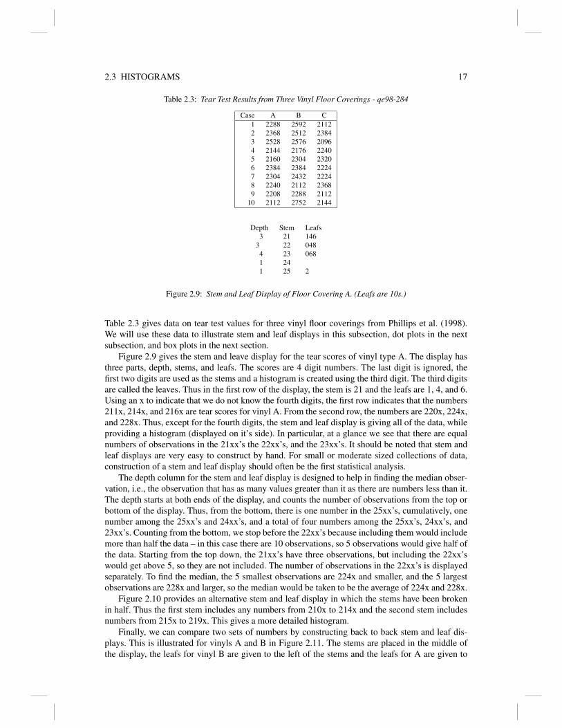
Table 2.3: Tear Test Results from Three Vinyl Floor Coverings - qe98-284

Case A B C1 2288 2592 21122 2368 2512 23843 2528 2576 20964 2144 2176 22405 2160 2304 23206 2384 2384 22247 2304 2432 22248 2240 2112 23689 2208 2288 2112

10 2112 2752 2144

Depth Stem Leafs3 21 146

3 22 0484 23 0681 241 25 2

Figure 2.9: Stem and Leaf Display of Floor Covering A. (Leafs are 10s.)

Table 2.3 gives data on tear test values for three vinyl floor coverings from Phillips et al. (1998).We will use these data to illustrate stem and leaf displays in this subsection, dot plots in the nextsubsection, and box plots in the next section.

Figure 2.9 gives the stem and leave display for the tear scores of vinyl type A. The display hasthree parts, depth, stems, and leafs. The scores are 4 digit numbers. The last digit is ignored, thefirst two digits are used as the stems and a histogram is created using the third digit. The third digitsare called the leaves. Thus in the first row of the display, the stem is 21 and the leafs are 1, 4, and 6.Using an x to indicate that we do not know the fourth digits, the first row indicates that the numbers211x, 214x, and 216x are tear scores for vinyl A. From the second row, the numbers are 220x, 224x,and 228x. Thus, except for the fourth digits, the stem and leaf display is giving all of the data, whileproviding a histogram (displayed on it’s side). In particular, at a glance we see that there are equalnumbers of observations in the 21xx’s the 22xx’s, and the 23xx’s. It should be noted that stem andleaf displays are very easy to construct by hand. For small or moderate sized collections of data,construction of a stem and leaf display should often be the first statistical analysis.

The depth column for the stem and leaf display is designed to help in finding the median obser-vation, i.e., the observation that has as many values greater than it as there are numbers less than it.The depth starts at both ends of the display, and counts the number of observations from the top orbottom of the display. Thus, from the bottom, there is one number in the 25xx’s, cumulatively, onenumber among the 25xx’s and 24xx’s, and a total of four numbers among the 25xx’s, 24xx’s, and23xx’s. Counting from the bottom, we stop before the 22xx’s because including them would includemore than half the data – in this case there are 10 observations, so 5 observations would give half ofthe data. Starting from the top down, the 21xx’s have three observations, but including the 22xx’swould get above 5, so they are not included. The number of observations in the 22xx’s is displayedseparately. To find the median, the 5 smallest observations are 224x and smaller, and the 5 largestobservations are 228x and larger, so the median would be taken to be the average of 224x and 228x.

Figure 2.10 provides an alternative stem and leaf display in which the stems have been brokenin half. Thus the first stem includes any numbers from 210x to 214x and the second stem includesnumbers from 215x to 219x. This gives a more detailed histogram.

Finally, we can compare two sets of numbers by constructing back to back stem and leaf dis-plays. This is illustrated for vinyls A and B in Figure 2.11. The stems are placed in the middle ofthe display, the leafs for vinyl B are given to the left of the stems and the leafs for A are given to

18 2. BASIC TOOLSDepth Stem Leafs

2 21 143 21 65 22 045 22 84 23 03 23 681 241 241 25 2

Figure 2.10: Alternative Stem and Leaf Display of Floor Covering A. (Leafs are 10s.)

B Stem A71 21 1468 22 048

80 23 0683 24

971 25 226

5 27

Figure 2.11: Back to Back Stem and Leaf Displays for Vinyls B and A of Floor Covering A. (Leafs are 10s.)

the right of the stems. It is clear that vinyl B tends to have larger tear results than vinyl A. However,the minimum tear results are nearly the same for both vinyls. Note that back to back stem and leafdisplays only allow comparison of two vinyls, and we have three vinyls in the data.

2.3.2 Dot Plots

Dot plots provide yet another form of histogram. They consist of a plot of an axis (scaled to beappropriate for the data) along with dots above the line to indicate each data point. Figure 2.12gives the dot plot for the tear test results for vinyl A.

Dot plots can be used to give a visual comparison of several groups of observations. Figure 2.12gives dot plots on a common scale for all three vinyls in Table 2.3. We can see that the observationsfor vinyl B tend to be a bit larger and perhaps more spread out than those for vinyls A and C. VinylsA and C look quite comparable except for one observation just over 2520 in vinyl A.

. . . . . . . . . .

-------+---------+---------+---------+---------+---------

2160 2240 2320 2400 2480 2560

Figure 2.12: Dot Plot of Floor Covering A.

A . .. . . .. . . .

-----+---------+---------+---------+---------+---------+-

B . . .. . . . .. .

-----+---------+---------+---------+---------+---------+-

C

.: . : . . . .

-----+---------+---------+---------+---------+---------+-

2160 2280 2400 2520 2640 2760

Figure 2.13: Dot Plots for Three Floor Coverings.

2.4 BOX PLOTS 19---------------------------

------I + I--------------------

---------------------------

--------+---------+---------+---------+---------+--------

2160 2240 2320 2400 2480

Figure 2.14: Box Plot of Floor Covering A.

Table 2.4: Summary Statistics

VinylCover MIN Q1 MEDIAN Q3 MAX

A 2112 2156 2264 2372 2528B 2112 2260 2408 2580 2752C 2096 2112 2224 2332 2384

2.4 Box Plots

Box plots give an alternative visual display of the data based on a five number summary of the data.

EXAMPLE 2.4.1 Vinyl Floor Covering Data.Figure 2.13 gives the box plot for the vinyl A data of Table 2.3. Note that the overall impression ofthe plot is one of symmetry. The mark in the middle of the box is near the center of the box, and thelines on the edges are not too dissimilar in length.

The five numbers on which box plots are based are the maximum observation, the minimumobservation, the median (the point that has half the data smaller than it and half the data larger), thefirst quartile Q1 (the point that has 1/4 of the data smaller than it and 3/4 of the data larger), andthe third quartile Q3 (the point that has 3/4 of the data smaller than it and 1/4 of the data larger).The plot makes a box using Q1 and Q3 as ends of the box, marks the median inside the the box, andcreates “whiskers” from the ends of the box out to the maximum and minimum. Many programs forcomputing box plots define inner and outer fences and identify two classes of outliers as points thatfall outside the inner and outer fences.

EXAMPLE 2.4.1 Vinyl Floor Covering Data continued.Table 2.4 gives the five summary statistics on which the box plots for the vinyls are created. Themedian for cover A is actually any number between 2240 and 2288 but it is reported as the mean ofthese two numbers.

To compare the vinyls visually, we can plot box plots for all three on a common scale. Fig-ure 2.14 reconfirms the impression that vinyls A and C are roughly similar, with vinyl C looking alittle smaller and more compact. Vinyl B tends to be larger and more spread out but having the samelowest observations.

While the length of the box plot is Q3−Q1, when plotting multiple box plots with very differentsample sizes it can be useful to use the square root of the sample size as the width of the box plot.McGill, Tukey, and Larsen, (1978) discuss this and other variations on box plots.

2.5 Cause and Effect Diagrams

Cause and Effect diagrams, also known as Fishbone and Ishikawa diagrams, are a useful qualityimprovment tool but are not really a statistical tool in that they do not involve analyzing numericaldata. Cause and Effect diagrams are just that, they diagram the potential causes of an effect. Thesepotential causes can then be explored to see what is the real cause of an effect. Usually, the effects

20 2. BASIC TOOLS------------------

A ----I + I--------------

------------------

-------------------------

B ---------------I + I--------------

-------------------------

------------------

C -I + I------

------------------

------+---------+---------+---------+---------+---------+

2160 2280 2400 2520 2640 2760

Figure 2.15: Box Plots for Three Floor Coverings.

Effect

Teacher

Exams

Students

Texts

Measurements

Environment

Cause and Effect (Fishbone) Diagram

Figure 2.16: Cause and Effect diagram with only primary causes.

of interest are somehow undesirable, the purpose of the cause and effect diagram is to brainstormpossibilities for fixing problems.

EXAMPLE 2.5.1 Figures 2 .15 and 2.16 illustrate cause and effect diagrams for a statistics class.At the end of the spine, is the effect of interest, the statistics class. On the primary ribs coming offof the spine are the Primary causes. In Figure 2.15 these are listed as the Students, the Teacher,The Text books, and the Exams. If Figure 2.16 additional detail is given to each primary cause,identifying secondary causes. For Students these are the course prerequisites, their home life, andtheir study habits. For the Teacher, these are the teacher’s knowledge, interest and communicationskills. Figure 2.17 presents the general idea.

2.6 Flow Charts

Flow charts (also known as process maps) are used to graphically display the steps in a process.Minitab has support for constructing flow charts, see

support.minitab.com/en-us/workspace/get-started/map-your-process/

2.6 FLOW CHARTS 21

Effect

comm. skills

level

study habits

home life

prereqs

grading

level

comm. skills

interest

knowledge

Teacher

Exams

Students

Texts

Measurements

Environment

Cause and Effect (Fishbone) Diagram

Figure 2.17: Fishbone diagram with both primary and secondary causes.

Flow charts can be made in R.A sophisticated package that allows easy construction is DiagrammeR. After loading the package

the following simple code illustrates three simple flow charts.library(DiagrammeR)

DiagrammeR("graph LR;

A-->B;

B-->C;

B->>D")

DiagrammeR("graph TB;

A(Rounded)-->B[Squared];

B---C{Rhombus!};

C-->D>flag shape];

C-->E((Circle));")

DiagrammeR("graph TB;

A(Both Working)-->B[One Working];

A-->C{Both \n Failed};

B-->A;")

Basic programing information is given athttps://cran.r-project.org/web/packages/DiagrammeR/DiagrammeR.pdf and the au-thor provides a video at http://rich-iannone.github.io/DiagrammeR/. I found out aboutthis fromhttps://sites.temple.edu/psmgis/2017/07/30/flow-charts-in-r-using-diagrammer/

An alternative is the R package diagram.

EXAMPLE 2.6.1 Figure 2.18

Chapter 3

Probability

3.1 Introduction

In this chapter we review the basic notions of probability. Simply put, probability models are usedto explain random phenomena. Before we define a probability, let us try to understand how proba-bilities are used and how probabilities are calculated.

Imagine that you are driving to work and you are interested in how many people are drivingthe same model car as you. Your experiment consists of counting cars of the same model that youencounter on your drive to work. The actual outcome of this experiment cannot be predicted withcertainty. The set of all possible outcomes is called the sample space and it is denoted by S. Forthis experiment, the sample space is S = {0,1,2, ...,500} where we assume that you encounter atmost 500 cars on your drive to work. Within the sample space, we can define events of interest. Forexample, you may want to make sure that your’s is a relatively exclusive model and you will believethis if you see only 0, 1, or 2 others like it. We would express this event as A = {0,1,2}. You maydecide that the masses are driving this car if you see 3 or more cars of the same model on the road.This event is expressed as B = {3,4,5,6,7...,500}.

Events are subsets of the sample space. Generally, we use capital letters from the beginning ofthe alphabet to denote events. In examples like this in which we can list the possible outcomes,probabilities are typically assigned to outcomes and are computed for events. Probabilities are al-ways between 0 and 1 and can posibly be either 0 or 1. Something that happens with probability 1is a sure thing and something that has no chance of happening has probability 0. Something mustalways occur, i.e. some outcome in the sample space must always occur because the sample spaceis a listing of everything that can occur. Therefore the probability of the sample space is 1. If someevent occurs with a certain probability, say 0.3, then the probability that it will not occur is 1−0.3.If two events are mutually exclusive, they cannot both happen at the same time. For example, onyour drive to work, if you count a total of 3 or more cars, then the event A = {0,1,2} cannot happen,because the event B has occurred.

The easiest way to compute probabilities are in situations where outcomes are equally likely. Weare all familiar with probability models such as tossing coins and rolling dice. In situations whereevery outcome in the sample space is equally likely, we compute the probability of an event E as

Pr(E) =number of outcomes in E

total number of outcomes in the sample space

This formula is a way of computing probabilities and is not a definition of probability. A rigorousdefinition of probability is quite difficult, as difficult as defining concepts such as force and velocityin physics.

We now examine an example in which the outcomes do not have equal probabilities.

EXAMPLE 3.1.1. Consider six outcomes having to do with your driving habits and the posibilityof you getting a speeding ticket. The outcomes are all combinations of two factors, first whether youget a speeding ticket (Y ) or do not get a speeding ticket (N) and second, whether you never driveover the speed limit (NDO), you sometimes drive over the speed limit (SDO), or you always drive

23

24 3. PROBABILITY

Table 3.1: Speeding–Getting a Ticket probabilities

SpeedingNDO SDO ADO

Speeding Y 0.0 0.18 0.30Ticket N 0.12 0.30 0.10

over the speed limit (ADO). The combinations of these factors define six possible outcomes. Theprobabilities are listed in Table 3.1.

Note that each of the probabilities is between 0 and 1 (inclusive) and that each outcome has adifferent probability. The probability of an event such as the event that you sometimes drive over(SDO) the speed limit is computed as

Pr(SDO) = Pr[(SDO,Y ) or (SDO,N)]

= Pr(SDO,Y )+Pr(SDO,N)

= 0.30+0.18= 0.48 .

Similarly, Pr(NDO) = 0.12 and Pr(ADO) = 0.40. These are called marginal probabilities (becausetypically they would be written in the margin of the table). The marginal probabilities for whetheror not you get a ticket are

Pr(Y ) = 0.48, Pr(N) = 0.52.

These computations are illustrations of the addition rule for probabilities. If A and B are eventsthat cannot happen simultaneously, e.g., you cannot simultaneously get a tecket and not get a ticketwhile sometimes driving over the speed limit, then Pr(A or B) = Pr(A)+Pr(B).

We can also compute conditional probabilities. These are probabilities of events that are condi-tional on the knowledge of some other event. In our example, suppose your beloved knows that yougot a ticket on your way to work and he/she claims that you always drive over the speed limit. Now,to defend yourself, you want to compute the probability that you always drive over (ADO) the speedlimit given that you received a ticket (Y). This is written Pr(ADO|Y ) and read as “the probabilityof ADO given that the event Y has occurred”. It is computed as the joint probability of the eventsADO and Y divided by the marginal probability of the event Y ,

Pr(ADO|Y ) = Pr(ADO,Y )Pr(Y )

=0.30.48

= 0.625.

Notice that the probability that you always drive over is Pr(ADO) = 0.4 but given that youreceived a speeding ticket, the conditional probability has jumped to 0.625. This says that the oc-currence of the event Y which tells your beloved (and anyone else) that you received a speedingticket, has provided them with additional information about your driving habits.

We say two events, A and B are independent if knowledge of one event provides no informationabout the other. In this case, the probability that both events occur is the product of their marginalprobabilities

Pr(A and B) = Pr(A)Pr(B).

In our example, we see that the event that you always drive over the speed limit is not independentof the event that you get a speeding ticket

Pr(ADO and Y ) = 0.3 6= (0.4 ×0.48) = Pr(ADO)Pr(Y ).

Another, more intuitive, way to check for independence is to see whether the conditional probability

3.2 SOMETHING ABOUT COUNTING 25

of an event is altered from its unconditional probability, e.g., is Pr(ADO|Y ) = Pr(ADO)? If theseprobabilities are the same, we say the events are independent. In our example Pr(ADO|Y ) = 0.625and Pr(ADO) = 0.4, so kowing the event Y occurs provides additional information about ADO, inthis case making ADO more probable. Generally, independence is a property that is assumed, notproven.

3.2 Something about counting

In order to define our sample space, we are interested in the number of ways in which somethingcan happen. Combinatorics is the field that is concerned with counting. For example, suppose youare interested in the number of ways that you can get dressed in the morning. Suppose you’re apoor college student and you own exactly 2 shirts that you plucked out of a dumpster, one is purpleand the other is orange. You also own 3 pairs of pants that were given to you by various lovingfamily members: their colors are fuschia, emerald, and poinsettia. Now, without regard to fashionor style, the number of ways that you can get dressed on this particular day is 6. For each shirtyou choose, there are 3 possible pairs of pants to choose and so you have 2 shirts × 3 pants = 6possible outcomes. Notice that if you were limited by concern about untoward fashion statements,your number of ways to get dressed would be different.

Our shirts and pants example is an illustration of the Multiplication Principle of Counting:Suppose we can select an object X in m ways and an object Y in n way. Then the pair of objects(X ,Y ) can be selected in mn ways.

EXAMPLE 3.2.1. New Mexico car license plates used to have 3 digits followed by 3 letters. Thetotal number of possible license plates without restriction is:

(10×10×10)× (26×26×26).

There are 10 choices for each number and 26 choices for each letter. Of course, New Mexico carlicence plates are limed by concern about untoward three letter verbal statements.

Suppose now that we are not allowed to repeat any number or letter. There are still 10 ways topick the first number but once that is picked, there are only 9 ways to pick the second number. Thenumber of possible license plates without repetition of a number or letter is:

(10×9×8)× (26×25×24).

Here, the order in which the items are selected is important. The licence plate 123 ABC is differentfrom the plate 213 CBA. An ordered arrangement of 3 similar items is called a permutation. Wewould not talk about a permutation in regard to a licence plate because it involves dissimilar items,both numbers and letters. We would talk about a permutation of the numbers (or the letters). Count-ing the number of licence plates without replications involves the 10×9×8 different permutationsof the ten numbers taken three at a time as well as the permutations of the 26× 25× 24 differentpermutations of the twenty six letters taken three at a time.

Permutation: The number of permutations of n objects taken k at a time is

Pnk = n(n−1)(n−2) · · ·(n− k+1).

A succinct way to write the right hand side of the above equation is

Pnk =

n!(n− k)!

where n!≡ n(n−1)(n−2) · · ·(2)(1) and 0!≡ 1. Our answer for the number of possible New Mexicolicense plates without repeating a number or letter can be re-expressed in this notation as

P103 × P26

3 = 11,232,000.

26 3. PROBABILITY

In New Mexico, there are plenty of licence plates for the number of cars, but one can see that in,say, California, problems might develop.

Often, we are interested in arrangements where order is not important. For example, supposeyour nutritious lunch box contains an apple, a tangerine, and a pear. If you cared about what orderyou ate them in, you would eat lunch in P3

3 = 3! ways. From the point of view of your taste buds,it matters which fruit you eat first, second and third. However, from the point of view of yourstomach, it merely gets a lump of all 3 fruit and therefore only one end result. This way of selecting3 fruit from 3 fruit without regard to order is called a combination. If you had 3 fruits available, butpromised a colleague first choice, so you only eat 2, there are three different lumps that could existin your stomach: [apple, tangerine], [apple, pear], and [tangerine, pear]. Recall that to your stomach[tangerine, pear] is the same combination as [pear, tangerine].

Combination: An unordered arrangement of k objects selected from n objects is called a combi-nation and is expressed as (

nk

)=

n!k!(n− k)!

.

In our two fruit example, (32

)=

3!2!(3−2)!

= 3.

A combination is a permutation with the number of ways to order the selected objects divided out.In our fruit example, there are P3

2 permutations but 2! ways to arrange the chosen fruit, therefore thecombination is P3

2 /(2!) = 3.

3.3 Working with Random Variables

A random variable links the outcomes of an experiment with numbers. When you roll a die, youlook at it and read off a number. The random experiment is rolling a cube that has dots marked onits various faces. The outcome is actually the face that ends up on top. Without even thinking aboutit, we look at the face and read off a number. The number is the random variable. Random variablesrepresent outcomes as numbers. The probabilities associated with outcomes are now transformed toprobabilities associated with the corresponding random number. When rolling a die, we discuss theprobability of getting a number from 1 to 6 rather than discussing the otherwise hard to describeoutcomes. Similarly, if we select a card from a deck of cards, say the one with seven hearts on it, werecognize that as a 7 and the suit as hearts. Numbers that are determined by random mechanismsare called random variables.

In this chapter we use capital letters from the end of the alphabet to denote random variablesand the corresponding lower case letters to denote their observed values. For example, the outcomesresulting from rolling a die can be represented by random variable X . X takes on any value from1,2,3,4,5,6. Once the die is rolled, we observe the outcome X = x, a specific value of X . If weobserve a 4, we write X = 4. We say the random variable X takes on the value x with probability1/6 since all of the outcomes are equally likely. This is written Pr(X = x) = 1/6 for x = 1, ...,6. Insubsequent chapters we will be more flexible in notation.

A random variable that has a finite or countable number of outcomes is called a discrete randomvariable. Since the outcomes can be listed, we can assign probabilities to each outcome. Randomvariables that yield random measurements typically do not have a countable number of outcomes.We can imagine the height of a person being 56.6πcm but we cannot count all such numbers.Random variables that can take on any value in some contiguous part of the real line are calledcontinuous random variables. For continuous random variables, we cannot list all the outcomesso we must assign probabilities in some other way. In fact, we assign probabilities to intervals ofnumbers. Of course, it is fairly obvious that all random variables we can measure must be discreterandom variables, because we are not capable of measuring heights like 56.6πcm. Nonetheless,

3.3 WORKING WITH RANDOM VARIABLES 27

Table 3.2: Probability mass function for X

x −2 0 3 4Pr(X = x) 0.25 0.1 .4 .25

when dealing with measurements, continuous random variables provide a valuable approximationto the extremely complicated discrete random variables that actually apply to measurements.

3.3.1 Probability Distributions, Expected Values

A probability distribution is a list of (numerical) outcomes and a means of specifying probabilitiesfor the events containing the outcomes. It assigns probabilities to the outcomes of random variableX . may need to explain this, not everyone may know. From elementary physics, we can think ofprobability as a mass spread over the possible outcomes of a random variable X . X has associatedwith it a center of gravity. This is called the expected value of the random variable. For a randomvariable X with a discrete number of outcomes x this is

E(X) = ∑all x

xPr(X = x).

E(X) is a weighted average of all possible values of X . The weights (masses) are the probabilities.

EXAMPLE 3.3.1. A computer program is used by the Psycho Fiends Brigade to bill people whocall their 1-900 number. The PFB’s software is a complicated Bayesian belief network, but it hasbugs in it. It charges 2 minutes less than a person called, the correct time, or either 3 or 4 minutesmore than was called. The incorrect billings caused by the Psyco Fiends network has the probabilitydistribution given in Table 3.2.

The expected value of X , written E(X), is a measure of the center of the random distribution. Itis computed as the weighted average of the outcomes x where the weights are given by the corre-sponding probabilities.

E(X) = ∑all x

xPr(X = x) = (−2)(0.25)+(0)(0.1)+(3)(0.4)+(4)(0.25) = 1.7.

On average, people are getting billed for 1.7 minutes more than they use. Thus, if the Psycho Fiendscharged everyone 1.7 minutes less, they might make the District Attorney’s office happy, although65% of their clients would still be upset over being billed too much.

On occasion, we need to compute the expected value of a function of X . For example E(X2) iscomputed as

E(X2) = ∑all x

x2Pr(X = x)

= (−2)2(0.25)+(0)2(0.1)+(3)2(0.4)+(4)2(0.25)= 8.6

In general,E[g(X)] = ∑

all x

g(x)Pr(X = x).

Note that on the left hand side of the equation, we take the expected value of a function of therandom variable X , say, g(X). On the right hand side, for each specific outcome x of X , we use g(x).

With regard to the Psycho Fiends call charges, the DA may care only about average charges, but

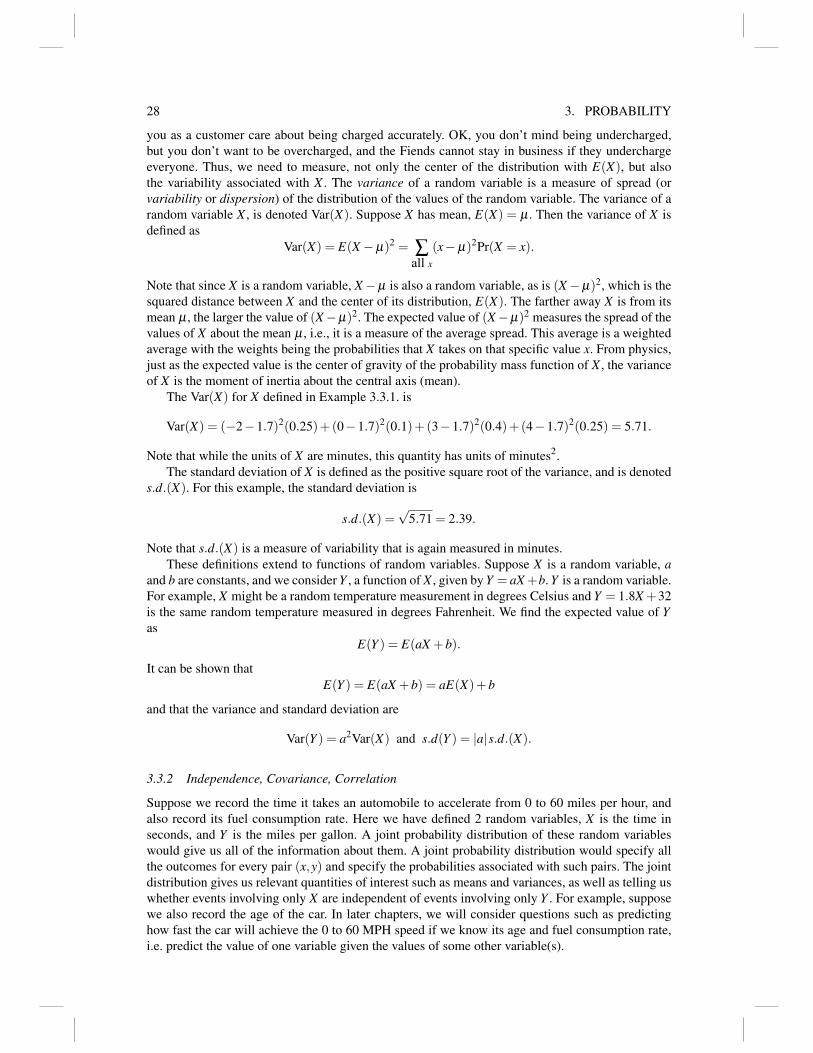
28 3. PROBABILITY

you as a customer care about being charged accurately. OK, you don’t mind being undercharged,but you don’t want to be overcharged, and the Fiends cannot stay in business if they underchargeeveryone. Thus, we need to measure, not only the center of the distribution with E(X), but alsothe variability associated with X . The variance of a random variable is a measure of spread (orvariability or dispersion) of the distribution of the values of the random variable. The variance of arandom variable X , is denoted Var(X). Suppose X has mean, E(X) = µ . Then the variance of X isdefined as

Var(X) = E(X−µ)2 = ∑all x

(x−µ)2Pr(X = x).

Note that since X is a random variable, X−µ is also a random variable, as is (X−µ)2, which is thesquared distance between X and the center of its distribution, E(X). The farther away X is from itsmean µ , the larger the value of (X−µ)2. The expected value of (X−µ)2 measures the spread of thevalues of X about the mean µ , i.e., it is a measure of the average spread. This average is a weightedaverage with the weights being the probabilities that X takes on that specific value x. From physics,just as the expected value is the center of gravity of the probability mass function of X , the varianceof X is the moment of inertia about the central axis (mean).

The Var(X) for X defined in Example 3.3.1. is

Var(X) = (−2−1.7)2(0.25)+(0−1.7)2(0.1)+(3−1.7)2(0.4)+(4−1.7)2(0.25) = 5.71.

Note that while the units of X are minutes, this quantity has units of minutes2.The standard deviation of X is defined as the positive square root of the variance, and is denoted

s.d.(X). For this example, the standard deviation is

s.d.(X) =√

5.71 = 2.39.

Note that s.d.(X) is a measure of variability that is again measured in minutes.These definitions extend to functions of random variables. Suppose X is a random variable, a

and b are constants, and we consider Y , a function of X , given by Y = aX +b. Y is a random variable.For example, X might be a random temperature measurement in degrees Celsius and Y = 1.8X +32is the same random temperature measured in degrees Fahrenheit. We find the expected value of Yas

E(Y ) = E(aX +b).

It can be shown thatE(Y ) = E(aX +b) = aE(X)+b

and that the variance and standard deviation are

Var(Y ) = a2Var(X) and s.d(Y ) = |a|s.d.(X).

3.3.2 Independence, Covariance, Correlation

Suppose we record the time it takes an automobile to accelerate from 0 to 60 miles per hour, andalso record its fuel consumption rate. Here we have defined 2 random variables, X is the time inseconds, and Y is the miles per gallon. A joint probability distribution of these random variableswould give us all of the information about them. A joint probability distribution would specify allthe outcomes for every pair (x,y) and specify the probabilities associated with such pairs. The jointdistribution gives us relevant quantities of interest such as means and variances, as well as telling uswhether events involving only X are independent of events involving only Y . For example, supposewe also record the age of the car. In later chapters, we will consider questions such as predictinghow fast the car will achieve the 0 to 60 MPH speed if we know its age and fuel consumption rate,i.e. predict the value of one variable given the values of some other variable(s).

3.3 WORKING WITH RANDOM VARIABLES 29

Table 3.3: Joint probability mass function

X−1 0 2

1 0.1 0 0.3Y 2 0 0.2 0

3 0.2 0 0.2

EXAMPLE 3.3.2. we need a story for this, why not the miles per gallon story. Suppose X andY have joint probability mass function given by Table 3.3. Here X is a measure of the number ofseconds it takes a car to go from 0 to 60mph where 0 indicates 30 seconds, -1 is 20 seconds, and 2is 50 seconds. Y is miles per gallon with 1 = 10mpg, 2 = 20mpg, etc.

We denote joint probabilities as Pr(X = x,Y = y) = p(x,y). So, p(−1,2) = 0, tells us that theprobability X = −1 and Y = 2 is 0. If we wanted only information about X from this joint massfunction, we would compute the marginal probability mass function (pmf) of X by summing out Y

Pr(X = x) = ∑all y

p(x,y).

For example, Pr(X =−1) = 0.1+0.2 = 0.3.We can extend the definition of independence of events to include independence of random

variables since random variables are based on events. Two random variables X and Y are indepen-dent if any events based on only X are independent of any events based on only Y . In other words,knowing anything about X does not change the probability for any event involving Y . In terms ofprobabilities, it is sufficient to have

Pr(X = x,Y = y) = Pr(X = x)Pr(Y = y).

In Example 3.3.2. , for X =−1 and Y = 1, we check independence

Pr(X =−1,Y = 1) = .1Pr(X =−1) = .3 and Pr(Y = 1) = 0.4

soPr(X =−1)Pr(Y = 1) = 1.2 6= 0.1 = Pr(X =−1,Y = 1).

Here are two events (X = 1) and (Y = 1) that are not independent, therefore X and Y are notindependent.

We can also see whether X and Y have any sort of linear relationship. The covariance is ameasure of linear relationship. Suppose X and Y are random variables with means µX and µY re-spectively, the covariance between X and Y is given by

Cov(X ,Y )≡ E[(X−µX )(Y −µY )] = ∑(x,y)

(x−µX )(y−µY )Pr(X = x,Y = y).

Note that a special case of this isCov(X ,X) = Var(X).

Another special case occurs when we have independence. If the random variables X and Y are inde-pendent, their covariance is 0. In general, the covariance can be positive or negative and its relativevalue depends on the units of X and Y . Positive covariances occur when large values of X occurwith large values of Y and small values of X occur with small values of Y . Negative covariancesoccur when small values of X occur with large values of Y and large values of X occur with smallvalues of Y . If X is the time in seconds to accelerate from 0 to 60 in our car example and Y is the

30 3. PROBABILITY

Table 3.4: Joint probability mass function

X−1 0 2 Pr(Y = y)

1 0.1 0 0.3 0.4Y 2 0 0.2 0 0.2

3 0.2 0 0.2 0.4Pr(X = x) 0.3 0.2 0.5 1

fuel consumption rate in MPG, and we compute the covariance between X and Y , the value shouldbe negative. Note that this covariance would change if we were to record Y in kilometers per litre.

To standardize the covariance measure, a unitless quantity called the correlation is defined,

Corr(X ,Y )≡Cov(X ,Y )/√

Var(X)Var(Y ).

The correlation is always a number between −1 and 1. The meaning of a correlation is the same asthat of a covariance but in addition, if the correlation between X and Y is 1, we say there is a perfectlinearly increasing relationship between X and Y . will probably cause confusion with earlier use ofX and Y If the correlation is −1, this is a perfect linearly decreasing relationship. A perfect linearrelationship between two random variables means that an increase of 1 unit in one random variableis associated with an exactly proportional change in the other. In our car example, this means that ifwe make a series of time observations on the car accelerating from 0 to 60 m.p.h and we record thefuel consumption rate in miles per gallon and kilometers per litre, the pairs of numbers should havea perfect linear relationship. We emphasize that the relationship is linear because the correlationdoes not identify perfect nonlinear relationships.

EXAMPLE 3.3.3. Let X and Y be random variables with joint probability mass function as definedin example 3.3.2, cf. Table 3.?. Then

E(X) = (−1)(0.3)+(0)(0.2)+(2)(0.5) = 0.7,E(Y ) = (1)(0.4)+(2)(0.2)+(3)(0.4) = 2,

Var(X) = (−1−0.7)2(0.3)+(0−0.7)2(0.2)+(2−0.7)2(0.5) = 0.81,Var(Y ) = (1−2)2(0.4)+(2−2)2(0.2)+(3−2)2(0.4) = 0.8,

Cov(X ,Y )

= (−1−0.7)(1−2)(0.1)+(0−0.7)(1−2)(0)+(2−0.7)(1−2)(0.3)= (−1−0.7)(2−2)(0)+(0−0.7)(2−2)(0.2)+(2−0.7)(2−2)(0)= (−1−0.7)(2−2)(0.2)+(0−0.7)(3−2)(0)+(2−0.7)(3−2)(0.2)= −0.3,

Corr(X ,Y ) =−0.3√

(0.81)(0.8)= −0.37.

This correlation is quite a bit larger that −1, but indicates that small values of X tend to occurwith large values of Y , as we can see from the probability distribution.

3.3.3 Expected values and variances for sample means

We now present some useful results for working with expected values, variances, and covariances oflinear combinations of random variables. All of the results presented here generalize to more than 2

3.3 WORKING WITH RANDOM VARIABLES 31

random variables. Suppose X1, X2, X3, and X4 be random variables and let a1, a2, a3, and a4 be realconstants.1. E(a1) = a1 and E(a1X1) = a1E(X1).2. E(a1X1 +a2X2) = a1E(X1)+a2E(X2).

3. Var(a1) = 0 and Var(a1X1) = a21Var(X1).

4. Var(a1X1 +a2X2) = a21Var(X1)+a2

2Var(X2)+2a1a2Cov(X1,X2).5. If X1 and X2 are independent, then Cov(X ,Y ) = 0. in which case 4 reduces to Var(a1X1+a2X2) =

a21Var(X1)+a2

2Var(X2)0.6. Cov(a1X1 +a2X2,a3X3 +a4X4) = a1a3Cov(X1,X3)

+a1a4Cov(X1,X4)+a2a3Cov(X2,X3)+a2a4Cov(X2,X4).

The most basic data we collect is a random sample from a population. These are just independentrandom observations on the same population. Since the populations are the same, these observationswill have the same distribution, which means that each of them would have the same mean (expectedvalue) and variance.

We now concentrate on a function of random variables that is very important is statistical infer-ence the sample mean. Let X1,X2, ...,Xn be random variables each with the same population meanE(Xi) = µ for i = 1, ...,n. The average of these random variables is also a random variable. Definethe sample mean as

X =X1 +X2 + · · ·+Xn

n.

We can find the expected value of this average of the random variables by finding the expected valueof the linear combination

E(X) = E(1n

X1 +1n

X1 + · · ·+1n

Xn)

=1n

E(X1)+1n

E(X2)+ · · ·+1n

E(Xn)

=1n

µ +1n

µ + · · ·+ 1n

µ (n terms)

=1n

nµ

= µ

When we have a random sample, we use X to estimate the population mean µ . The fact that E(X) =µ indicates that X is a reasonable estimate of µ .

If we assume further that X1,X2, ...,Xn are independent and have the same variance, say,Var(Xi) = σ2 for i = 1, ...,n, we can compute the variance of X

Var(X) = Var(1n

X1 +1n

X2 + · · ·+1n

Xn)

=(1

n

)2Var(X1)+

(1n

)2Var(X2)+ · · ·+

(1n

)2Var(Xn)

=1n2 σ

2 +1n2 σ

2 + · · ·+ 1n2 σ

2 (n terms)

=1n2 nσ

2

=σ2

n

The variance of X is the variance of an individual observation, Var(Xi) divided by n. When we

32 3. PROBABILITY

have a random sample, σ2/n gives a measure of the variability of X as our estimate of µ . Morecommonly, we use the standard deviation s.d.(X) = σ/

√n. Regardless of the measure, X has much

less variability than an individual observation Xi (depending on the size of n). Ultimately, aftercollecting data we compute X which means we we get to look at one observation on X . Because Xhas less variability, that one observation on X is likely to be closer to µ than if we were to look at asingle observation, say X1.

Define the sample variance as

S2 =(X1− X)2 +(X2 +−X)2 · · ·+(Xn− X)2

n−1.

The rules for expected values can be used to establish that

E(S2) = σ2,

although doing so is more laborious than our results for the sample mean. The degrees of freedom(df) for a variance estimate is an index of how much information is in the estimate. For the samplevariance the degrees of freedom are n−1 because there are n observations but we lose one degreeof freedom for not knowing E(Xi) = µ and replacing it with its estimate X . In Chapters 4 and 9 wewill average several independent variance estimates so their degrees of freedom will be the sum ofthe df for the individual estimates.

3.4 Binomial Distribution

Certain distributions arise repeatedly in statistical applications. These distributions are given names.The binomial distribution is one that arises when we have a fixed number of independent and identi-cal random trials that result in one of two types of outcomes. (Binomial comes from roots meaningtwo names.) We are interested in the random numbers of each type of outcome. Note that with afixed number of trials, if we know the number of times one outcome occurs, we can immediatelyfigure out the number of the other outcome. Examples are

testing a batch of identical components and counting the number of components that pass (orfail) the test,checking airline scheduling accuracy and counting the number of flights that left on time.checking whether a community meets the standards for group immunity against measles, andcounting the number of people who have been vaccinated against measles

Each of these situations has only two possible outcomes. Generally, these are termed successes orfailures. To understand the distribution of the number of successes in these situations, consider thefirst example. Suppose we have a batch of 4 resistors and we are going to test each one to see whetheror not it works. Each resistor is a trial. The probability that a resistor is good is p and the probabilitythat a resistor is bad is 1− p. We usually call the outcome we are interested in a “success”. In thiscase, Pr(success) = p and the probability of the complementary event, Pr( f ailure) = 1− p. LetX count the number of good resistors, so X can take on the values 0,1,2,3,4. Define events G =resistor is good and D = resistor is defective. The event {X = 0} means that none of the resistorsare good. Using the independence of the resistors, we find the probability X = 0 as

Pr(X = 0) = Pr(DDDD)

= Pr(D)Pr(D)Pr(D)Pr(D)

= (1− p)(1− p)(1− p)(1− p) = (1− p)4.

The event {X = 1} means that one of the resistors is good and the other 3 are defective. Thiscan happen in many ways. We can think of this as the number of ways to select one good resistor

3.4 BINOMIAL DISTRIBUTION 33

Table 3.5: Probability mass function for the number of good resistors

X Pr(X = x)0

(40

)p0(1− p)4

1(4

1

)p1(1− p)3

2(4

2

)p2(1− p)2

3(4

3

)p3(1− p)1

4(4

4

)p4(1− p)0

from the resistors. Using the addition rule and independence, Pr(X = 1) is

Pr(X = 1)= P{ GDDD or DGDD or DDGD or DDDG }= Pr(GDDD)+Pr(DGDD)+Pr(DDGD)+Pr(DDDG)

= p(1− p)3 +(1− p)p(1− p)2 +(1− p)2 p(1− p)+(1− p)3 p

= 4p(1− p)3

=

(41

)p(1− p)3.

The Pr(X = 2) is the probability of having 2 good resistors.

Pr(X = 2)= P{GGDD or GDGD or DGGD or DGDG or DGGD or DDGG}= Pr(GGDD)+Pr(GDGD)+Pr(DGGD)

+Pr(DGDG)+Pr(DGGD)+Pr(DDGG)

= 6p2(1− p)2

=

(42

)p2(1− p)2,

where the last line is given as an alternative to get the probability. Rather than listing each outcome,we can think of the number of ways of having 2 defective resistors in 4 resistors,

(42

)= 6. The

probability of any one of these outcomes with 2 good and 2 bad resistors is p2(1− p)2 and there are6 ways that this can happen. We compute the remaining probabilities in the same manner and theyare listed in Table 3.5.

In general, we do not want to list every single outcome every single time we have a situationlike this, and especially not if the number of trials n is large! The general functional form for thistype of probability distribution, called the binomial distribution is

Pr(X = x) =(

nx

)px(1− p)n−x, for x = 0,1, ...,n, 0≤ p≤ 1.

We use the notation X ∼ Bin(n, p) to mean that random variable X is binomially distributed withparameters n and p.

EXAMPLE 3.4.4. When one of us was a student, she owned a car that was designed such thatevery time it rained, water leaked through and took out a fuse or 2 or 3. Fortunately, she lived inthe desert, but in any case, she was forced to buy fuses in boxes of 10. On any given box, therewas a warranty that stated that she could get her money back if 2 or more fuses were defective. Theprobability that a fuse is defective is .01. What is the probability that she would get my money back?

First check to see whether this fits a binomial situation. There are n = 10 fuses. Each fuse is a

34 3. PROBABILITY

trial. We can reasonably assume for the moment that the fuses are defective independently of oneanother. Each fuse is defective with probability p = 0.01. Let X count the number of defective fusesin a box, then X ∼ Bin(10, .01). The event {X ≥ 2} is the event that the money-back warranty wouldhave to be honored. So we find Pr(X ≥ 2)

Pr(X ≥ 2) = Pr(X = 2)+Pr(X = 3)+Pr(X = 4)+ · · ·+Pr(X = 10).

It is easier to look at the complementary event

Pr(X ≥ 2) = 1−Pr(X ≤ 1)= 1− [Pr(X = 0)+Pr(X = 1)]

= 1−[(

100

)(0.01)0(1−0.01)10+

(101

)(0.01)1(1−0.01)9

]= 0.004

The mean and variance of X ∼ Bin(n, p) are difficult to compute from the definitions in Subsec-tion 3.3.1, but are quite simple to compute using results from Subsection 3.3.3. We merely state theresults:

E(X) = np Var(X) = np(1− p).

Note also from the definition of a binomial, that if X1 ∼ Bin(n1, p) and independently X2 ∼Bin(n2, p) then X1 +X2 ∼ Bin(n1 +n2, p).

mean and variance of a binomial. sums of binomials.

3.5 Poisson distribution

A probability distribution that is closely related to the Binomial is called the Poisson distribution.The Poisson distribution is used to model the occurrence of very rare events, e.g., rare diseases andthe number of defects in high quality products. While the proportion of defects may be very small,when there are a very large number of trials the number of defects that occur can be substantial. Anadvantage of the Poisson distribution is that it can be used to model product defects when we haveno clear idea of the number of units that have been produced that could be defective. For example,one might consider the number of painting defects on a piece of sheet metal. How many locationsare there for the painting to be defective? Innumerable. The probability of having a painting defectat any one point is very small but the number of defects can still be substantial.

Suppose we have a binomial with a very large number of trials n and a very small probabilityof occurrence p. Since n is large and p is small, their product, which is the expected number ofdefectives, can be of moderate size, say µ = np. The binomial variance is np(1− p) = µ(1− p) butsince p is very small, 1− p is essentially 1 and the variance is essentially µ . In other words, if Yhas a Poisson distribution with parameter µ , write Y ∼ P(µ). The expected value is E(Y ) = µ andVar(X) = µ .

3.6 Normal Distribution

Often, our random variables of interest are continuous. Ideally, a continuous random variable cantake on any value in an interval. The actual value of such a variable is limited by the precision ofthe measuring instrument. Examples are time, temperature, weight, and strength. All are measuredto the nearest unit. When we say that the temperature is 70◦F , we mean that it is somewhere in aninterval about 70◦F , say between 69.5◦ and 70.5◦. There are many continuous distributions that areuseful for modeling continuous data. The most common of these is the normal distribution.

The normal distribution arises naturally in many physical experiments. In particular, the normaldistribution can provide a close approximation to both the Binomial and Poisonn distributions whentheir expected values are reasonably large.

3.6 NORMAL DISTRIBUTION 35

Discuss standard normal and need for more generality. Examples and pictures, Maybe use theroller coaster riders.

Chapter 4

Control Charts

In this chapter, we examine control charts. Control charts are used to establish whether a process isin statistical control. Theoretically, a process is in statistical control when it generates a sequenceof random observations that are independent with the same statistical distribution for each obser-vation (iid). Unfortunately, it is impossible to tell whether a process is iid by observing it. Controlcharts provide an operational definition (one that can be checked against observations) for whetherobservations are close enough to iid for us to treat them as such. Since we are not proving thatthe observations are iid, we define the process to be under control when the operational definitionis satisfied. Here we discuss components for a definition of “under control” that have been founduseful historically, along with their statistical motivations. Essentially, we use observable propertiesof iid sequences to define what it means to be under control.

Control charts are merely plots of the data or data summaries with control limits superimposedon the plots. The control limits are used to identify processes that are out of statistical control. Con-trol charts were developed by the founder of statistical quality control, Walter A. Shewhart.His ideas were systematically introduced in Shewhart (1931). The ultimate goal of establishing thata process is under statistical control is that it provides a basis for making accurate predictions aboutthe future product from the process.

EXAMPLE 4.0.1 Table 4.1 contains 50 observations on a person’s diastolic blood pressure. Thisis actually a subset of a collection of 460 blood pressures taken on this individual twice each dayas reported by Shumway (1988). The individual in question determines a process for producingdiastolic blood pressures. We will investigate these 50 observations to examine whether the processis in statistical control. We will also consider control charts for blood pressures that were measuredfour times on a regular basis but were not measured every day. Diastolic blood pressures of 94 orgreater are considered high; we will also consider control charts that examine the frequency of highblood pressure values. 2

Control limits are based on a simple idea. Let y be a random data point, let the population meanof such observations be E(y) = µ , and let the population variance be Var(y) = σ2 so that the pop-ulation standard deviation is σ . Control limits are based on the fact that y will very probably fallbetween µ − 3σ and µ + 3σ . If y happens to follow a normal distribution, the probability of be-ing in this interval is 99.7%. Chebeshev’s inequality ensures that the probability is always at least

Table 4.1: Diastolic Blood Pressures

0 1 2 3 4 5 6 7 8 900 105 92 98 98 98 95 92 94 92 9210 95 92 94 93 98 96 92 94 98 9120 92 90 88 97 93 95 96 84 93 9230 94 90 90 85 94 90 95 94 95 8540 94 92 94 92 92 90 94 90 85 90

Read across and then down.

37

38 4. CONTROL CHARTS

1−(1/32).= 88.9% and, under weak conditions discussed in Pukelsheim (1994) or briefly in Chris-

tensen (1996, Section 1.3), this can be raised to 1− [(2.25)32]−1 .= 95.1%. When an observation

does not fall within the interval, something unusual, i.e., a special cause has occurred. (Commoncauses are those that determine the inherent variability of the process and can only be controlled bymanagement.) Control charts differ depending on the exact nature of the datum y. Often, the datumis actually the average of several observations. Sometimes the datum is the number of defectivesamong a fixed number of items. Sometimes the datum is the number of defectives in a large butunspecified number of items. Moreover, µ and σ are, in practice, unknown and must be estimated.Various control charts use different estimates of µ and σ .

It is not our goal to give an exhaustive discussion of control charts but rather to present examplesthat introduce some of the main ideas and types of control charts in a simple manner. To this end,we use notation that is consistent with the rest of the book but therefore is less consistent withtraditional discussions. We also present charts that are simple but less commonly used. Rather thanillustrating all of the more commonly used charts, we often merely discuss their differences fromthose presented here. For a detailed discussion of control charts see, for example, Ryan (1989).

Control charts and the corresponding control limits have clear connections to statistical predic-tion intervals and statistical tests. The charts are computed using assumptions that, ideally, should besubjected to verification. We could clearly do more sophisticated analyses than control charting butat the danger of intimidating and even driving away users of statistics. Control charts should perhapsbe viewed as simply a plot of the data along with an estimate of the average level of the process anda rough measure of how much variability one reasonably expects to see. In practice, control chartsare often used by people with a minimum of statistical training. They are rough and ready (quickand dirty?) procedures. In practice, the choice is often between a simple data analysis and no dataanalysis. Moreover, one can, and probably should, take a different philosophical approach to controlcharts that calls in question the association with statistical tests and prediction intervals. We returnto the philosophical issue later.

Basically the operational definition of whether a processes is under control is that it stays withinthe control limits of• a means chart and a dispersion (s, R, or S2) chart for rational subgroup data or• an individual chart and moving range chart for individual observations or• a p, Np, c or u chart for attribute data.To that operational definition one can add extra conditions like those described in Nelson (1984) orpossibly versions of EWMA charts or CUSUM charts. All of these procedures are discussed in thischapter.

Perhaps more important than the details of constructing control charts is getting people to graphtheir data and look at it.

4.1 Individuals Chart

EXAMPLE 4.1.1 An I (individuals) chart. Consider the single sample of data presented in Ta-ble 4.1. From these data compute n = 50, y· = 92.880, and s = 3.799. We want control limits ofµ±3σ . These are estimated with y·±3s so the estimated upper control limit is

UCL = 92.880+3(3.799) = 104.277

and the estimated lower control limit is

LCL = 92.880−3(3.799) = 81.483.

The control chart is displayed in Figure 4.1. The plot displays all of the observations, the upperand lower control limits are given as horizontal lines, and a horizontal line is used to indicate theestimated mean value of 92.88.

4.1 INDIVIDUALS CHART 39

Figure 4.1: I (Individuals) Chart for Table 4.1.

We will defer a detailed discussion of interpreting control charts until the next example but notethat the very first observation is beyond (apparently on) the upper control limit and that four of thefirst five observations are at a substantial distance above the mean line. Both of these facts indicatethat the process is not in control. To get the process under control, some action is needed. Perhapsthe initial high readings are due to the patient going on a beer, licorice, and salted peanut binge justbefore the study started. This is one possible explanation for the process being out of control. Otherpossible explanations must be sought out.

Traditionally, the sample standard deviation s is not used for estimating σ in this control chart.The traditional method involves going through the data and averaging the distances between adja-cent data points (moving ranges). (Recall that distances are always positive.) This average distanceis then divided by a tabled adjustment factor to give an estimate of σ . Alternatively, the sample stan-dard deviation s is sometimes divided by a different tabled adjustment factor to give an unbiasedestimate of σ . In deriving all of the estimates of σ , the observations are assumed to be independent.In addition, the tabled adjustment factors both depend on the data being normally distributed. Theassumption of independence is frequently a bad one for data used in control charts and we will seelater that it is a particularly bad assumption for the diastolic blood pressure data.

Figure 4.2 gives a control chart based on the moving ranges. It is a plot of the distances betweenconsecutive observations and is designed to evaluate whether the variability of the process remainsconstant. The average of the moving ranges can be used to develop an alternative estimate of thestandard deviation that is not as liable to bias due to a shift in the process mean but it requiresan assumption of normal data. The center line is the mean of the moving ranges and the standarddeviation of a moving range is a multiple of σ and so is estimated using a tabled multiplier of themean moving range. (This can all be related to the theory behind Tukey’s HSD multiple comparisonmethod.) Minitab commands for control charts are given in Section 4.8. 2

Alternatively, the variance can be estimated by the squared distance between consecutive points(squared moving ranges),

σ2 ≡ 1

2(n−1)

n−1

∑i=1

(yi+1− yi)2.

40 4. CONTROL CHARTS

Figure 4.2: Moving Range Chart for Table 4.1.

This can be shown to haveE(σ

2)= σ2.

If the process is subject to a mean shift at some time, as a function of the moving ranges, σ2 issubject to far less bias due to the mean change than is s2.

The key point from Example 4.1.1 is that when the process is out of control, action must be takento bring the process under control before attempting to improve the process by reducing variability.As with any control chart, once the process is brought under control, the control chart needs to berecomputed.

4.2 Means Charts and Dispersion Charts

Perhaps the most commonly used control charts are based on data collected in rational subgroups.An example of such data is given in Table 4.2. This contains 19 groups of four blood pressurereadings. The four readings were taken under essentially identical conditions. Two charts are tradi-tionally constructed: one that plots the means for the various samples and one that plots the rangesof the various samples. Recall that the range of a sample is simply the largest observation in thesample minus the smallest observation in the sample. The means chart is a tool to identify changesin the process mean but it can also show changes in process variability. In Subsection 9.1.2 we willdiscuss the ability of the means chart to detect lack of independence. The range chart is designedto examine the process variability. Alternatives to the range chart are the sample standard deviationchart and the sample variance chart. In the next example, we examine the means chart, the samplestandard deviation chart, and the range chart. The last two of these are typically referred to as s andR charts, respectively. The means chart is traditionally called an X (X-bar) chart but we always usey for the variable being analyzed, so we would refer to this as a y chart. (Software may label themas X or X-bar.)

The standard advice is that one should never interpret a means chart unless a correspondingdispersion chart (range, standard deviation, or variance) has already established that the variabilityis under control. While means charts are sensitive to a lack of control in the variability of the process,

4.2 MEANS CHARTS AND DISPERSION CHARTS 41

Table 4.2: Nineteen Samples of Diastolic Blood Pressures

Group Data Mean Std. Dev. Rangei yi1 yi2 yi3 yi4 N yi· si Ri1 105 92 98 98 4 98.25 5.32 132 95 96 84 93 4 92.00 5.48 123 90 97 97 90 4 93.50 4.04 74 90 88 86 90 4 88.50 1.915 45 100 92 92 90 4 93.50 4.43 106 78 82 82 84 4 81.50 2.52 67 90 83 83 87 4 85.75 3.40 78 95 85 88 90 4 89.50 4.20 109 92 90 87 85 4 88.50 3.11 7

10 84 85 83 92 4 86.00 4.08 911 90 87 84 90 4 87.75 2.87 612 93 88 90 88 4 89.75 2.36 513 92 94 87 88 4 90.25 3.30 714 86 87 91 88 4 88.00 2.16 515 90 94 94 82 4 90.00 5.66 1216 95 95 87 90 4 91.75 3.95 817 96 88 90 84 4 89.50 5.00 1218 91 90 90 88 4 89.75 1.258 319 84 82 90 86 4 85.50 3.42 8

Total 76 89.434 4.848 7.947

to know whether a problem identified in a means chart is a problem with the level of the process ora problem with variability, one needs to examine both charts.

EXAMPLE 4.2.1 The data in Example 4.1.1 are actually a subset of 460 blood pressure mea-surements. The complete data were sampled to obtain the data given in Table 4.2. Frequently it isimpractical or wasteful to take measurements on every item produced. Going to a doctor’s officetwice every day to have your blood pressure measured is certainly very inconvenient and is likelyto be quite expensive. (Much nicer to buy your own wrist cuff.) To simulate realistic sampling froma process, the 460 observations were divided into 18 consecutive groups of 25 with a final group of10. The first four observations from each group were taken as the sample from the group. The dataare given in Table 4.2 along with the group mean, standard deviation, and range.

This method of obtaining data is similar in spirit to evaluating an industrial process in which aworker produces 25 units per day and measuring the first four units produced each day. Alternativesampling schemes might be to sample units produced at four specified times during the day or totake a random sample of four units from the 25 produced in a day. If one samples at specified timesof day, the times may need to be worked into the analysis, in which case the data structure woulddiffer from Table 4.2. In any case, the groups must be formed in some rational manner. Shewhartemphasized that they should be taken under essentially identical conditions. This leaves room fordetecting effects that appear when conditions are not identical. (Sampling at specified times of day toform a group is a bad idea if the process can change in the course of a day.) Shewhart also suggestedthat one should probably have 25 or more groups (more than our 19 groups) before declaring aprocess to be under control, i.e, we can potentially find our process to be out of control but nomatter what the data tell us we should be hesitant to say that it is under control.

The last row of Table 4.2 includes the sample standard deviation of the 76 observations com-puted by ignoring the group structure, 4.848, and the grand mean of all observations, y·· = 89.434,which is used to estimate µ . It also contains the mean of the sample ranges, R = 7.947. The pooledestimate of the variance σ2 is just the average of the s2

i s. This is often called the mean squared error(MSE). The value is 14.48 and the pooled estimate of σ is

√MSE = 3.81.

42 4. CONTROL CHARTS

Figure 4.3 Means Chart for the (i, yi·) data of Table 4.2 using√

MSE. (The label at the top of the chart iscreated by Minitab and refers to the four columns of numbers in the table that are yi1 through yi4.)

Note that for an iid process, if we select groups of observations from the process using any selec-tion criteria that does not depend on the actual values of the observations, then each datum is anindependent observation from the process (population).

The control chart for the sample means is given in Figure 4.3. For a process under control, atypical observation yi j is assumed to have mean E(yi j) = µ and Var(yi j) = σ2. The observationsplotted in the control chart are the group mean values yi·. The mean values have E(yi·) = µ butVar(yi·) = σ2/4 because there are 4 observations in each mean. The upper and lower control limitsare determined by the standard deviation of yi· which is σ/2. The control limits are µ ± 3(σ/2).Using the estimated parameters from the previous paragraph, the estimated control limits become

UCL = y··+3

√MSE

4= 89.434+3

3.812

= 95.15

and

LCL = y··−3

√MSE

4= 89.434−3

3.812

= 83.72.

In general, if each sample has size N, the estimated control limits are

y··±3

√MSE

N.

Using the MSE as an estimate of σ2 assumes that the observations within each group are uncor-related (or independent). This is often a poor assumption; we will return to it later. (Independencebetween groups of observations is not crucial but, oddly, because groups tend to be more widelyseparated in time or other factors, the assumption of independence between groups is frequentlyreasonable.)

The control chart in Figure 4.3 is nonstandard. More commonly, estimates of σ other than√MSE are used. The alternative estimates involve using tabled adjustments. The tabled adjustments

assume that the observations within each group are both independent and have normal distributions.Often, σ is estimated by the average of the sample ranges, R = 7.947, divided by a tabled constant.

4.2 MEANS CHARTS AND DISPERSION CHARTS 43

This estimate is unbiased because, for independent normal observations, the expected value of therange of a sample is σ times this constant that depends only on the sample size. Alternatively, σ issometimes estimated by

√MSE divided by a tabled constant. Although MSE is an unbiased estimate

of σ2,√

MSE is not an unbiased estimate of σ . The tabled constant corrects for the bias that occurswhen the observations are independent and normal. (Even though a little statistical bias is not reallysuch a bad thing in an estimate.) The means chart using the bias corrected estimate of σ based on√

MSE is very similar to Figure 4.3 because, with a large number of degrees of freedom for error,the bias correction factor is very close to one. (The degrees of freedom for MSE is the sum of the dffor each s2

i , hence is n(N−1).)Traditionally, means charts use R in estimating σ and R charts are used to evaluate dispersion.

Interestingly, Shewhart (1931) never uses such charts. I presume their use was popularized becauseranges are easier to calculate by hand than standard deviations but also because, for small groupsizes like N = 4, the inefficiency introduced by using the range is small. (Although Mahmoud etal., 2010, take strong exception to this statement.) Ranges should not be used unless group sizes arevery small and, with the accessibility of electronic calculation, there seems to be little point in everusing ranges. (Moving ranges for individuals are another story.)

As discussed earlier, we have to know the distribution of the yis to know the probability that anindividual observation, one that is under control, will appear to be under control. If we are plottingobservations with normal distributions, the probability is 99.77%. Chebeshev’s inequality assures usthat the probability is at least 88.9% and, with additional assumptions, at least 95%. One advantageof means charts is that means tend to have distributions more like the normal than do individual(unaveraged) observations. Thus we can be more confident of having a relatively large probabilityof identifying means as being under control when they truly are under control.

Return now to interpreting Figure 4.3. Two of the observations, the first and the sixth, are beyondthe control limits. The first three points and cases 3, 4, and 5 both have the property that two of thethree consecutive points are more than two standard deviations above the center line of 89.43. (Twostandard deviations above the center line is 89.43+(2/3)(95.15− 89.43) = 93.24). Each of theseevents is highly unlikely when the group means are independent and normally distributed. Moreover,four of the first five points are more than one standard deviation above the center line. Again, thisevent is highly unlikely if the group means are independent and normally distributed.

As mentioned earlier, we should not interpret the means chart unless a corresponding dispersionchart establishes that the variability is under control. We now examine dispersion charts for thesedata. We will see that the dispersion seems to be controlled.

Figure 4.4 is a control chart of the sample standard deviations. It is used to detect changes in thevariation of the process. The points plotted are just the sis from Table 4.2. The center line at 3.521is just

√MSE times the ratio of two bias adjustment factors.

√MSE is divided by one adjustment

factor to get an unbiased estimate of σ and then multiplied by another adjustment factor so thatthe center line has the same bias as the sis that are being plotted. In this way, the center line isan estimate of the expected value of the sis. The control limits are the expected value of si plusand minus three times the standard deviation of si. For independent and normally distributed data,the standard deviation of si is a tabled multiple of σ that depends on the group sample size. Theestimated control limits are 3.521 plus and minus three times the tabled value times the estimateof σ . Sometimes, as in this chart, the computed lower control limit is a negative number. Standarddeviations cannot be negative so in such cases the lower control limit is taken to be zero. The s chartshows no lack of control.

The R chart in Figure 4.5 is an alternative control chart for detecting changes in the variationof the process. In this chart the ranges of the samples, as reported in Table 4.2, are used to indicatevariability. The center line of the chart is the average of the sample ranges from Table 4.2, R =7.947. The control limits are the expected value of a range plus and minus three times the standarddeviation of a range. For independent and normally distributed data, the standard deviation of arange is a tabled multiple of σ that depends on the group sample size. The estimated control limitsin Figure 4.5 are 7.947 plus and minus three times the tabled value times the estimate of σ . In

44 4. CONTROL CHARTS

Figure 4.4: s Chart for the (i,si) data of Table 4.2.

Figure 4.5: R Chart for the (i,Ri) data of Table 4.2.

this chart, the estimate of σ was taken as the appropriate multiple of R. As with the s chart, if thelower control limit is negative, it is adjusted to zero because a range cannot be negative. The R chartdisplays no lack of control. 2

Although they do not seem to be as popular as s and R charts, mathematically it is easy to createa variance (s2) chart. If the variance in each group is the same,

σ2 = E(MSE) = E(s2

i ),

so the chart plots the pairs (i,s2i ) with center line MSE. With independent normal observations,

4.2 MEANS CHARTS AND DISPERSION CHARTS 45

(N− 1)s2i /σ2 has something known as a chi-squared distribution with N− 1 degrees of freedom,

written(N−1)s2

i /σ2 ∼ χ

2(N−1).

From properties of the χ2(N−1) distribution we get

(N−1)E[s2i ]/σ

2 = N−1 and (N−1)2Var[s2i ]/σ

4 = 2(N−1).

From this it follows that

E[s2i ] = σ

2 and Var[s2i ] = 2σ

4/(N−1).

(The first of these holds without the normality assumption that leads to the chi-squared distribution.)Estimating σ2 with MSE we get control limits of MSE±3MSE

√2/(N−1) and no need for finding

correction factors.

There are several criteria (tests) commonly used with control charts to evaluate (determine)whether a process is under control.

1. The first test is obviously whether any points fall beyond the control limits. (Shewhart refers tothis as Condition I.)

2. A second indication is the existence of 9 or more consecutive points on the same side of thecenter line.

3. A third indication is a trend of 6 or more points that are all increasing or decreasing. (Someauthors require 7 points for a trend.)

4. A periodic, up and down cycling in the plot indicates nonrandomness and lack of control. Having14 consecutive points that alternate up and down, i.e., no three points are increasing or decreas-ing, indicates a problem.

5. Too many, say 15, consecutive points within one standard deviation of the center line is a prob-lem.

6. Having 8 consecutive points beyond one standard deviation of the center line is another problem.7. Having two of three consecutive points beyond two standard deviations is a problem.8. Having four of five consecutive points on the same side of the center line and beyond one standard

deviation is a problem.

For more details, see Nelson (1984).1

In constructing means charts, Shewhart (1931) emphasizes that the observations must be dividedinto rational subgroups that have data generated under essentially identical conditions. Rationalsubgroups must be determined by the subject matter. If the observations are taken in time sequence,it is rational to group observations made at similar times. If 100 observations are the result ofhaving four observations on each of 25 workers, it is rational to group the observations by worker.Shewhart (1931) also emphasizes the use of small subgroups because they are sensitive to fleetingchanges in the process. N = 4 observations per group is very commonly used. Shewhart (1939, p.37) recommends that one have at least 25 groups of 4 observations that appear to be in controlbefore drawing the conclusion that a process is under control.

Control charts are used for two purposes: process analysis and process control. In our exampleswe discuss process analysis. We have past data on a process and seek to determine whether theprocess was in control when the data were obtained. Process control also uses past data to form acontrol chart but the center line and control limits are extended into the future so that new data canbe plotted as they arrive. As long as the new data are consistent with a process in control, the process

1Stationary processes as discussed in Chapter 6 are “under control” but could easily violate these conditions.

46 4. CONTROL CHARTS

is allowed to continue. When the new data indicate that the process is out of control, the process isadjusted to put it back in control. When the process is adjusted, control charts must be recomputed.

Once the process is under control, the goal should be to reduce variability while keeping theprocess on target, i.e., focused on the ideal specification. Staying on target is usually easier toachieve than reducing variability.

The data used for constructing a means chart has the same structure as data used in one-wayanalysis of variance, cf. Section 9.1. Also, Ott’s Analysis of Means procedure, cf. Christensen (1996,Subsection 6.5.1), provides a test for equality of means that is directly related to means charts.

4.2.1 Process Capability

In many applications, notably industrial production, a process is required to produce items thatmeet certain specifications. Typically, these specifications come in the form of specification limitsthat items must fall between. It becomes of considerable importance to recognize whether a processis capable of meeting such specifications. Processes that are not under control have no capability tomeet any specifications.2 The capability of a process that is under control is defined to be µ ± 3σ .The process can be expected to produce items within these limits. If the observations are indepen-dent and normally distributed, 99.7% of the items produced will fall within the µ ± 3σ interval. Ifthe interval defined by the specification limits contains the process capability interval, the processis capable of meeting specifications. In other words, if the upper specification limit is above µ +3σ

and the lower specification limit is below µ−3σ , the existing process will meet the specifications(at least 99.7% of the time for normal, independent data). If the specification interval partially over-laps or misses the process capability interval, the process needs to be changed before it can meetspecifications. Until the process is brought under control with the capability of meeting specifica-tions, all items produced must be inspected individually to see whether they meet specifications.When the process is controlled and capable, none of the items need to be inspected.

The process capability is estimated to have limits.

y·±3s or y··±3√

MSE,

or the same formula incorporating bias adjustments for s or√

MSE. For individuals, these are justthe estimated control limits. An estimated process capability is also easily obtained from a meanschart. The control limits in a means chart are µ ± 3σ/

√N where N is the group sample size. The

process capability limits are µ ± 3σ . The difference between the two control limits is 6σ/√

N.Multiplying this difference of 6σ/

√N by

√N/2 gives 3σ from which it is easy to obtained the

process capability. To illustrate the computations, reconsider the means chart in Figure 4.3. Recallthat the blood pressure process is not under control, so the process has no capability. We are merelyillustrating the computations for process capability. The difference between the control limits inFigure 4.3 is 95.15−83.72 = 11.43. In Figure 4.3, N = 4, so the estimate of 3σ is 11.43(

√4/2) =

11.43. The estimated process capability would be the value of the center line, 89.43, plus and minusthe estimate of 3σ . From Figure 4.3, the process capability would be estimated as 89.43± 11.43,i.e, the interval from 78.00 to 100.86 (if this process were under control and had a capability).

Figure 4.6 contains Minitab’s process capability chart. As far as I can tell, this figure does notactually compare the capability limits to the specification limits. In the left box LSL and USL arethe lower and upper specification limits, respectively, set here as blood pressures of 55 and 94. Atarget blood pressure was not specified. Below these in the left box are numbers related to the sum-maries from Table 4.2: the grand mean y··, the total sample size 19×4 = 76, a bias adjusted

√MSE

[StdDev(Within)], and the bias adjusted overall sample standard deviation computed from all 76observations. (The bias adjustments converge to 1 when the sample sizes – technically the degrees

2To be predictable, a process need only be stationary, not iid. Positively correlated stationary processes would haveartificially narrower control limits, hence a greater probability of getting outside the limits. BUT the justification for thesecontrol limits is not a probability statement but the experience that they work!

4.2 MEANS CHARTS AND DISPERSION CHARTS 47

Figure 4.6: Process Capability Chart for the Data of Table 4.2

of freedom – get large and in this example the “overall” adjustment is negligible.) In the boxesbelow the graph, PPMs are parts per million (rather than percentages or estimated probabilities).The observed performance is just that. The expected within and overall performances are based onapproximating normal distributions using the grand mean and an estimated standard deviation (ei-ther within or overall). The stuff in the right box are commonly used measures that I have not yetdecided are worth caring about. For example, this Cp statistic is the length of the specification inter-val divided by the length of the process capability interval, so a value greater than 1 tells you thatyou could potentially meet specifications if you were exactly on target. The other “C” measures arerefinements on Cp. (This Cp is not the commonly used Mallows’ Cp created for variable selectionin regression.)

4.2.1.1 Six-Sigma

There has been much discussion of achieving 6σ process control. There is a narrow focus of 6σ

which is merely an aspect of process capability. There is also a general focus with Six-Sigma beingthe name of a quality management program, see Hahn et al. (1999) and the January 2002 issue ofQuality Progress.

As an aspect of process capability, the 6σ concept has sometimes been misunderstood. Whenmisunderstood, 6σ can easily lead to lowering the quality of products. For a process under control,the capability remains the µ±3σ limits. Properly understood, 6σ limits have been achieved whenthe specification interval contains the limits µ ± 6σ . This can only happen when σ is very smallrelative to the variability allowed with the specification limits.

If the specification limits happen to be 3σ from the mean µ , so they happen to agree with thecontrol limits, with normal data about 0.3% (3 out of 1000) units will be outside of specifications.If the variance has been reduced so that now the specification limits agree with µ± 6σ , almost nounits will be outside specifications. Anytime the µ ± 6σ limits are within the specification limitsyour “process capability” is fantastic. (But you could potentially do even better in overall quality bymoving µ closer to the specified target, say µ0.)

The point is that 6σ is something to be achieved by reducing variability – which is very difficult.If 6σ is somehow imposed rather than being achieved, it has almost certainly been misunderstood

48 4. CONTROL CHARTS

Table 4.3: High Blood Pressure Readings

# of HighGroup (i) N Pressures (yi) pi

1 25 13 0.522 25 10 0.403 25 9 0.364 25 3 0.125 25 2 0.086 25 2 0.087 25 2 0.088 25 2 0.089 25 1 0.04

10 25 0 0.0011 25 1 0.0412 25 1 0.0413 25 3 0.1214 25 2 0.0815 25 11 0.4416 25 4 0.1617 25 1 0.0418 25 1 0.04

Total 450 68 0.151

and the misunderstanding is ruining quality. For example, making the incorrect claim that a processis under control whenever observations are within µ±6σ will have disastrous results.

As a method of quality management, Six-Sigma focuses on using quality methods to improvefinancial measures – something that is probably inevitable for a successful program given the natureof American business management.

4.3 Attribute Charts

Frequently, control charts are used to evaluate whether certain attributes of a process are undercontrol. We now consider such charts.

EXAMPLE 4.3.1 Np chartDiastolic blood pressures are considered to be high if they are 94 or larger. To illustrate what areknown as Np charts, we dichotomized the 460 blood pressure observations into pressures that werehigh and those that were not. Further we divided the 460 observations into 18 consecutive groups of25 while ignoring the last 10 observations. The data are given in Table 4.4. The values for pi in thetable are simply the observed proportions of high blood pressures, i.e., the number of high pressuresdivided by 25. An Np control chart is a plot of the number of high blood pressures versus the group.The chart is given in Figure 4.7.

If the 460 observations have the same distribution, there is some fixed probability p that anobservation will be 94 or greater. If the observations are all independent, then the number of highpressures out of each group of 25 has a binomial distribution, i.e., the number of high counts yihas yi ∼ Bin(N, p) where N = 25 is the number of trials in each group. As seen in Section 3.4,E(yi) = Np, Var(yi) = Np(1− p), and the standard deviation of yi is

√Np(1− p). It follows that the

center line for the Np chart is at Np and the control limits are at Np±3√

Np(1− p). As mentioned,N = 25, but we do not know p and must estimate it. We combine information across groups. FromTable 4.4 there are a total of 68 high blood pressure readings out of 450 total readings, so the totalestimate of p is 68/450 = 0.151. The center line is estimated as 25(0.151) = 3.778. (Note that thecenter line value can also be computed as the number of high blood pressures averaged over the 18groups, i.e., 68/18.) The control limits are 3.778± 3

√25(0.151)(1−0.151). The number of high

4.3 ATTRIBUTE CHARTS 49

Figure 4.7: Np Chart for High Diastolic Blood Pressures

Figure 4.8: p Chart for High Diastolic Blood Pressures

blood pressures is nonnegative so if the computed lower control limit is negative, the limit is takenas 0. Similarly, the number of high blood pressures cannot be larger than N = 25.

From the Np chart, the process is obviously out of control. Three points are above the controllimits while there is a string of 11 consecutive points that are below the center line. It should alsobe noted that, as with other charts, the attribute data for this chart was obtained by forming rationalsubgroups. We looked at the numbers of high readings in groups of 25 consecutive observations.And again, we have only 18 groups rather than Shewhart’s suggested 25 so even if the process werenot out of control, we would be hesitant to claim that it was in control. 2

50 4. CONTROL CHARTS

It is not always the case that one has the same number of trials in each group. The yis couldbe yi ∼ Bin(Ni, p) where the Nis change from group to group. In such cases the Np chart can bemodified but the modified chart will not have a horizontal center line. In these cases it is convenientto form a p chart. In a p chart, the proportions (the pis) are plotted against the group identifier.The center line of the plot is the pooled estimate of p, i.e., the total number of events divided bythe total number of trials. For the high blood pressures, the pis from Table 4.4 would be plottedagainst group number with a center line at 68/450 = 0.151. In this plot, the upper and lower controllimits may vary from group to group. For group i, pi has E(pi) = p and Var(pi) = p(1− p)/Ni.Thus the estimated control limits for the number of high blood pressures in a group of, say, Ni =10 measurements are 0.151± 3

√0.151(1−0.151)/10. Different groups with different numbers

of trials Ni will have different control limits. For Ni = 10, the estimated upper limit is 0.49. Theestimated lower limit is −0.19 which is adjusted to 0. If the proportion of high readings among10 measurements is greater than 0.49, in other words if 5 or more of the 10 readings are high, theprocess is out of control.

EXAMPLE 4.3.2 p chartFigure 4.8 gives the p chart for the data of Table 4.3. Because the Nis all equal 25, it looks just likethe Np chart except all the entries are divided by 25. The following exercise adds more data andchanges the results. 2

EXERCISE 4.1 Shumway gave 460 BP readings. The first 450 are summarized in Table 4.3. Thefinal 10 readings contain 0 high blood pressures. Reconstruct the p chart incorporating this extragroup of data.

Example 4.3.4 also contains a p chart with substantial variation in the Nis.The final types of control charts that we will discuss in any detail are c and u charts. These

charts are based on count data having a Poisson distribution. Poisson data are similar to Binomialdata with small probabilities of detecting an attribute but many trials in which to detect them. Forexample, the number of defects on the surface of a table might have a Poisson distribution where theprobability of a defect at any location is small but there is no obvious limit to the number of locationson the table surface. If yi is Poisson, and E(yi) = µ , then µ determines the entire distribution and inparticular Var(yi) = µ .

The c chart involves plotting the number of occurrences versus the “group.” (A group may bea single object like a table.) The center line is µ , which is identical to that in the Np chart. µ isestimated as the average number of defects per group. The control limits are µ ± 3

õ and are

estimated by replacing µ with its estimate.

EXAMPLE 4.3.3 c chart.We illustrate the c chart by once again using the data of Table 4.3. These data are more properlyanalyzed with an Np or p chart but the sample sizes are not small and the probability of gettinga high blood pressure reading is not large, so the application is not too inappropriate. As in theNp chart, numbers of high readings are plotted against groups. As in the Np chart, the center line is3.778. It is the average number of high readings per group, 68/18 = 3.778. In the c chart, the controllimits are 3.778±3

√3.778 as opposed to the Np chart values of 3.778±3

√3.778(1−0.151). Even

though the sample sizes of N = 25 are not terribly large and the estimated probability 0.151 is notterribly small, the c chart given in Figure 4.9 is very similar to the Np chart in Figure 4.7. The uppercontrol limit is noticeably higher in Figure 4.9 but we still see three points above the UCL and 11consecutive points below the center line. 2

Variations on the c chart are also necessary. For example, when looking at the number of paintingdefects on a piece of sheet metal, if we have different sized pieces of sheet metal we need to adjustfor that fact. These adjustments are made in what are known as u charts. Suppose the observations yi

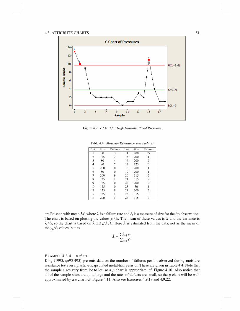
4.3 ATTRIBUTE CHARTS 51

Figure 4.9: c Chart for High Diastolic Blood Pressures

Table 4.4: Moisture Resistance Test Failures

Lot Size Failures Lot Size Failures1 80 3 14 200 272 125 7 15 200 13 80 4 16 200 94 80 7 17 125 05 200 0 18 200 16 80 0 19 200 17 200 9 20 315 58 125 1 21 315 29 125 0 22 200 0

10 125 0 23 50 111 125 8 24 200 212 125 1 25 315 313 200 1 26 315 3

are Poisson with mean λ`i where λ is a failure rate and `i is a measure of size for the ith observation.The chart is based on plotting the values yi/`i. The mean of these values is λ and the variance isλ/`i, so the chart is based on λ ± 3

√λ/`i. Here λ is estimated from the data, not as the mean of

the yi/`i values, but as

λ ≡ ∑ni=1 yi

∑ni=1 `i

.

EXAMPLE 4.3.4 u chart.King (1995, qe95-495) presents data on the number of failures per lot observed during moistureresistance tests on a plastic-encapsulated metal-film resistor. These are given in Table 4.4. Note thatthe sample sizes vary from lot to lot, so a p chart is appropriate, cf. Figure 4.10. Also notice thatall of the sample sizes are quite large and the rates of defects are small, so the p chart will be wellapproximated by a u chart, cf. Figure 4.11. Also see Exercises 4.9.18 and 4.9.22.

52 4. CONTROL CHARTS

Figure 4.10: p Chart for moisture resistance failures.

Figure 4.11: u Chart for moisture resistance failures.

4.4 CONTROL CHART SUMMARY 53

4.4 Control Chart Summary

Suppose we have data on a process yh, h = 1, . . . ,n. If the process is under control, any manner ofselecting the data, as long as the selection does not depend on the yh values, should provide a randomsample from the process. In other words, the yhs should be independent and identically distributed(iid). Unfortunately, we cannot look at a group of numbers and tell whether they are observationsfrom an iid process. The point of control charts is to create an operational definition of what it meansto be iid. If the control chart is satisfied, then the data are close enough to iid for us to use them forreliable prediction.

Control charts constitute an operational definition, not a statistical test, but like a statisticaltest, they are set up assuming things about the data, in this case that the data are iid. The idea is thatif the data are not iid, the control charts have a good chance of spotting the problem. We assumethat for h = 1, . . . ,n,

E(yh) = µ, Var(yh) = σ2.

Most often µ and σ2 are two unrelated, unknown parameters but in some problems (for attributedata) σ2 is actually a function of µ .

If the process is under control (i.e., if the observations are iid) then it should remain (largely)within the interval having the (control) limits

µ±3σ .

These limits also define the process capability. If the process capability interval is contained withinthe specification limits associated with the product, we are good to go. A process that is out of controlhas no capability!! The “Six-Sigma” program is named for the requirement that µ ± 6σ be withinthe specification limits. Such a requirement necessitates both reduced variability and (usually) thatthe target µ be near the center of the specification limits.

A key idea, perhaps the key idea, behind control charts is dividing the data into rational sub-groups having essentially identical conditions. When that is done, it becomes convenient to replacethe subscript h with a pair of subscripts i j wherein i identifies the rational subgroup and j identifiesobservations with the group. Rewrite the data as yi j, i = 1, . . . ,n, j = 1, . . . ,Ni. Here we must have atotal sample size of N1 + · · ·+Nn. As before,

E(yi j) = µ, Var(yi j) = σ2.

As discussed earlier, Shewhart recommends n≥ 25.From within each subgroup, we define a statistic of interest, say θi ≡ θi(yi1, . . . ,yiNi). These are

typically the sample mean, sample standard deviation, or perhaps the sample range. The statistic ofinterest is chosen so that the expected value is the same for every group, say,

E(θi) = θ

but the variance may depend on the group size, so write

Var(θi) =Vi.

A theoretical control chart would plot the pairs (i, θi), with a central horizontal line at θ and controllimits

θ ±3√

Vi.

In many charts, Vi is the same for all i, which makes for a more attractive chart. In practice, we needto estimate both θ and the Vis.

As discussed in Section 2, in addition to requiring that the plotted points remain within thecontrol limits, there are a number of other criteria that one may incorporate into the operationaldefinition of a process being under control.

54 4. CONTROL CHARTS

Table 4.5: Control Chart Summary. σ estimated by√

MSE, i.e., not bias corrected.

Chart θi θ θ√

Vi√

Vi NotesMeans yi· µ y··

√σ2/Ni

√MSE/Ni

Variance s2i σ2 MSE 2σ

2

Ni−12MSENi−1

S si cN−1σ cN−1√

MSE√

CN−1σ2√

CN−1MSE N ≡ N1 = · · · = Nn

R Ri dNσ R√

DNσ2√

DNMSE N ≡ N1 = · · · = Nn

NP yi ≡ Nyi· Np≡ nµ N p = Ny··√

N p(1− p)√

N p(1− p) N ≡ N1 = · · · = Nn

P pi ≡ yi· p≡ µ p = y··√

p(1−p)Ni

√p(1− p)

Ni

C yi µ µ ≡ ∑yi/n≡ y· ]sqrtµ√

µ yi ∼ Pois(µ)

U yi/`i λ λ ≡ ∑yi/∑`i√

λ/`i

√λ/`i yi ∼ Pois(λ`i)

Table 4.5 summarizes the standard control charts within this context. In the Np and p attributecharts we assume that the yi js only take on the values 0 and 1. The U and C charts essentially haveNi =∞ but that causes no problem. The dispersion/variability charts all incorporate values that areonly valid for data with normal distributions. In particular, the use of the χ2 distribution and comput-ing the bias constants cNi−1, CNi−1, dNi , and DNi all involve assuming the yi j have normal distribu-tions. With (Ni−1)s2

i /σ2 ∼ χ2(Ni−1), write cNi−1 as the constant for which E(si) = cNi−1σ . WriteCNi−1 for the value with Var(si) =CNi−1σ2. Write dNi for the value such that E(Ri) = dNiσ and DNi

for the value with Var(Ri) = DNiσ2. I am happy to estimate σ with

√MSE and have done so in the

table. Some people, including the makers of Minitab, prefer to estimate σ with√

MSE/c∑Ni−n, soone could change the table accordingly. Also, when N ≡ N1 = · · ·= Nn one could alternatively useR/dN as the estimate of σ .

As discussed in Chapter 6, a process that generates iid data is not the only process for whichreliable predictions can be made. If the process is stationary, the associated data will also be pre-dictable. Informally, a stationary processes is one in which, no matter when you choose to startlooking at the process, future and past observations always show the same patterns. For this to betrue, the mean and variance cannot change with time, but the observations do not have to be inde-pendent. In practice we can only evaluate past data, but we can look at “future” data relative to somepoint in the past. An iid process is always stationary, but stationary processes need not be iid. It ismuch more difficult to give an operational definition for a general stationary process than for an iidprocess. One needs to be very careful if trying to claim that a process that fails control charts is stillpredictable because the control chart failure is due to the process being stationary but not iid.

4.5 Average Run Lengths

When testing statistical hypotheses, tests are often evaluated by their size and power. The size is theprobability of rejecting an hypothesis when it is true and the power is the probability of rejectingan hypothesis when it is false. The average run length is a related concept for control charts. Therun length is the (random) number of points you plot until you see a point that is out of control. Theaverage run length is the expected value of the random run length. We want the average run lengthto be large for processes that are under control and short for processes that are out of control. TheEWMA and CUSUM charts in Section 7 were developed to have shorter average run lengths for outof control processes.

4.6 DISCUSSION 55

4.6 Discussion

Control charts are really designed as an operational definition of what it means for a process to beunder control. Not infrequently, statisticians want to interpret them as statistical tests for whetherthe mean of the process has jumped from its historical/previous value or for whether the data displaytrends, i.e., whether the mean of the process is gradually increasing or decreasing. Two useful pro-cedures for conducting such tests are CUSUM (cumulative sum) charts and EWMA (exponentiallyweighted moving average) charts and are discussed in the next section.

In a statistical test one makes a series of assumptions and checks to see whether the data areconsistent with those assumptions. Most often, a particular assumption is isolated as the null hy-pothesis and if the data are inconsistent with the assumptions we conclude that the null hypothesisis false. Logically, concluding that the null hypothesis is false requires us to believe that the otherassumptions are valid.

The whole point of control charting is to decide whether the data are independent observationsfrom a fixed process (population). It is not difficult to jump to the conclusion that this is an assump-tion we wish to test. However, one can take a very different philosophical view. One can take theview that the problem is not one of testing the assumptions but rather one of defining the terms usedin the assumptions. What does it actually mean for, say, 50 observations to be independent from thesame population. If we have an operational definition of what these terms mean, we will be able tolook at 50 numbers and decide whether they are independent observations from the same populationor not. The philosophy behind control charts is not to test ill defined assumptions but rather to givean operational definition of statistical control, see Shewhart (1939, p. 40). A person looks at variouscharacteristics of a control chart and if they are appropriate one concludes that the process satisfiesthe operational definition of being in statistical control. This is not too different from the philosophyfrequently adopted in Statistics. Typically, we do an informal check of mathematical assumptionsand, if the assumptions are not too bad, we proceed with formal statistical inferences, i.e, tests,confidence intervals, and prediction intervals. The only real difference is that in control charting,the checks on mathematical assumptions are formalized into an operational definition while the in-ferences are informal prediction intervals. It is of interest to note that typically informal checks onassumptions do not include methods for checking independence, whereas we will see in Subsec-tion 9.1.1 that means charts (and, it turns out, Np, p, c, and u charts) are effective at detecting lackof independence when rational subgroups have been chosen.

As pointed out above, many of the characteristics of traditional control charts (bias adjustments,variances of dispersion measures) are calculated by using results that relate to independent normallydistributed data. It follows that normal distributions are being built into the operational definitions ofstatistical control whereas normality is not part of the mathematical definition of statistical control.In our earlier discussion we were somewhat critical of this feature. From the philosophical point ofview presented here, our earlier discussions about the validity of assumptions need to be recast asdiscussions on the nature of an appropriate operational definition for statistical control.

Deming (1986, Chapter 11) alludes to these issues. On pages 334 and 335 he seems to suggestthat one should just use control charts without worrying about whether the data satisfy the assump-tions underlying the calculations. But earlier, on page 319, he indicates that usable decision rulesmust be made in advance and that the 3σ control limits work well “under a wide range of unknow-able circumstances”. In fact, I believe he is saying that one needs operational definitions and thatthe 3σ control limits have been found to provide a useful definition. More generally, Deming arguesthat a major problem in economic activities is that management fails to provide workers with opera-tional definitions and consequently, workers never know whether they have done a task successfully.Shewhart (1939) discusses these issues in more detail.

56 4. CONTROL CHARTS

4.7 Testing Mean Shifts from a Target

Control charts (with or without the additional criteria discussed by Nelson, 1984) are used to createan operational definition for what it means to have a process under control. We now present twosequential statistical tests for whether a process is on target at a specified value µ0. Only if you letthe data empirically determine the value µ0 can these be considered as potential additional criteriafor whether a process is under control, because being under control has nothing to do with being ontarget.

Exponentially weighted moving average (EWMA) charts and Cumulative Sum (CUSUM) chartsprovide sequential tests for whether a process experiences a mean shift away from a target. We willdiscuss the tests in terms of a sequence of observations y1,y2,y3, . . . ,yn that are independent andhave the same variance σ2. Let E(yi) = µi. The tests assume a null hypothesis that the means remainstable throughout the process at a fixed target value E(yi)= µ0. These procedures are good at pickingup the alternative that, up to some time T , the mean remains on target E(yi) = µ0, i = 1, . . . ,T butthen the entire process shifts slightly off target so that now E(yi) = µ0+δ , i = T +1, . . . ,n for somesmall δ 6= 0. They work best when T is small. The process control versions of these tests are moresensitive than individuals (or means) charts when δ is relatively small.

Both procedures can be used for process control using the empirical choice µ0 = y·, similarin spirit to the eight tests discussed by Nelson (1984). In fact, except at the beginning of the datasequence, EWMA charts do not depend heavily on the value µ0, so if you get past the first fewobservations an EWMA chart can be used as a criterion for process control even without empiricallychoosing µ0.

When applied to individual observations yi, the variance σ2 is estimated as it would be inan individuals chart. However both procedures can also be applied to a sequence of mean valuesy1·, y2·, y3·, . . . obtained from rational subgroups of size N. In this case the variance of an “obser-vation” σ2 is replaced by Var(yi·) = σ2/N and σ2 is well estimated by pooling the within groupsample variances.

4.7.1 Exponentially Weighted Moving Average Charts

Exponentially weighted moving average (EWMA) charts are a tool often used alongside controlcharts but they are really tests for whether the data display a mean shift away from a target µ0. Thechart uses the specified center line µ0 and plots the EWMA over time while checking whether theEWMA remains within 3 standard deviations of the center line.

For the purpose of constructing an EWMA chart, an EWMA is commonly defined via the recur-sive relationship

µt ≡ (1−α)yt +αµt−1,

where 0 < α < 1 and µ0 ≡ µ0. It is by no means clear what this has to do with an exponentiallyweighted moving average.

The obvious way to define an EWMA is to apply exponentially decreasing weights to eachobservation, i.e., for 0 < α < 1,

µt ≡ (αyt +α2yt−1 +α

3yt−2 + · · ·+αty1)/ t

∑i=1

αi =

∑ti=1 α iyt−i+1

∑ti=1 α i .

The point of this is that older observations get multiplied by much smaller numbers. We will latershow that when t is large, µt very nearly satisfies the recursive definition for µt and we will giveexplicit formulae for µt that display exponential downweighting of older observations.

As will be shown later, the standard deviation for µt with a fixed starting point µ0 is

σ

√(1−α

1+α

)(1−α2t).

4.7 TESTING MEAN SHIFTS FROM A TARGET 57

Figure 4.12: Exponentially weighted moving average chart for grouped diastolic blood pressures.

Typically, one just rejects the constant mean hypothesis whenever a plotted value gets outside of3 estimated standard deviations from the target µ0. The plot displays all of these results for t =1,2,3, . . . ,n. Note that as t gets large, the standard deviation rapidly approaches the limit

σ

√(1−α

1+α

).

The variance σ2 is estimated as in the individual charts of Section 4.1 or, when appropriate, themeans charts of Section 4.2. Lucas and Saccucci (1990) facilitate the construction of more formaltests.

Of course one needs to specify the value of α . A common default choice is α = 0.8. Manydiscussions of EWMA charts are presented in terms of

λ ≡ 1−α,

in which case the common default choice is λ = 0.2.To turn the “on target” test of H0 : µi = µ0, i = 1, . . . ,n into an under control test of H0 : µi = µ ,

i = 1, . . . ,n for come unspecified µ , we use µ0 = y·, the empirical choice. When doing so, peopletypically use the same variance formula ignoring the fact that y· is now random. One obvious alter-native choice is to start the recursion with µ1 ≡ y1, for which the variance will be given in the nextsubsection.

To a great extent, the niceties of turning the “on target” EWMA test into an under control cri-terion can be ignored because the exponential weighting soon discounts the target value µ0 out ofthe picture. For the first few steps t, the procedure is sensitive to whether E(yt) = µ0, but beforelong the chart essentially reduces to a test of whether there is a constant mean for all observationsor whether at some point in time the mean shifts.

Figure 4.12 gives the empirically centered EWMA chart with α = 0.8 for the grouped bloodpressure data of Table 4.2. Because it is grouped data the value of σ in the formulae should bereplaced with

√MSE/N or possibly a bias corrected version of that.

58 4. CONTROL CHARTS

4.7.1.1 Derivations of results

Three fundamental equalities about power series are needed. The first is obtained by looking at eachterm in the product (1−α)∑

∞i=0 α i,

11−α

=∞

∑i=0

αi,

α

1−α=∞

∑i=1

αi,

and finally,

t

∑i=1

αi =

∞

∑i=1

αi−

∞

∑i=t+1

αi

=∞

∑i=1

αi−α

t+1∞

∑i=0

αi

=α

1−α−α

t+1 11−α

=α−α t+1

1−α

.=

α

1−α,

when t is large.We can now see that µt approximately satisfies the recursive relationship that defines µt when t

is large.

µt ≡ ∑ti=1 α iyt−i+1

∑ti=1 α i

=αyt +∑

ti=2 α iyt−i+1

(α−α t+1)/(1−α)

.=

αyt +∑ti=2 α iyt−i+1

α/(1−α)

= (1−α)yt +∑

ti=2 α iyt−i+1

α/(1−α)

= (1−α)yt +α∑

ti=1 α iyt−1−i+1

α/(1−α)

.= (1−α)yt +α

∑t−1i=1 α iy(t−1)−i+1

α−α t/(1−α)

= (1−α)yt +αµt−1.

Assuming the data are uncorrelated (or independent) with E(yt) = µ and Var(yt) = σ2,

Var(µt) = Var(

∑ti=1 α iyt−i+1

(α−α t+1)/(1−α)

)=

∑ti=1 α2iVar(yt−i+1)

[(α−α t+1)/(1−α)]2

= σ2 ∑

ti=1 α2i

[(α−α t+1)/(1−α)]2

= σ2 (α

2−α2t+2)/(1−α2)

[(α−α t+1)/(1−α)]2

4.7 TESTING MEAN SHIFTS FROM A TARGET 59

= σ2(

α2−α2t+2

(α−α t+1)2

)((1−α)2

1−α2

)= σ

2 α2−α2t+2

(α−α t+1)2

(1−α

1+α

)= σ

2(

1−α2t

(1−α t)2

)(1−α

1+α

)= σ

2(

1+α t

1−α t

)(1−α

1+α

).= σ

2(1−α)/(1+α).

When t is small it pays to use the exact formula.From the recursive definition of µt that starts with µ1 = y1,

µt = (1−α)yt +αµt−1

= (1−α)yt +α [(1−α)yt−1 +αµt−2]

= (1−α)yt +α(1−α)yt−1 +α2µt−2

= (1−α)yt +α(1−α)yt−1 +α2 [(1−α)yt−2 +αµt−3]

= (1−α)yt +α(1−α)yt−1 +α2(1−α)yt−2 +α

3µt−3

= (1−α)yt +α(1−α)yt−1 +α2(1−α)yt−2 +α

3 [(1−α)yt−3 +αµt−4]

= (1−α)t−2

∑i=0

αiyt−i +α

t−1µ1

= (1−α)t−2

∑i=0

αiyt−i +α

t−1y1.

This involves exponential weighting but not as clearly as µ . Again assuming the data are uncorre-lated with E(yt) = µ and Var(yt) = σ2,

Var(µt) = Var

((1−α)

t−2

∑i=0

αiyt−i +α

t−1y1

)

= (1−α)2t−2

∑i=0

α2iVar(yt−i)+α

2(t−1)Var(y1)

= σ2

[(1−α)2

t−2

∑i=0

α2i +α

2(t−1)

]

= σ2

[(1−α)2

α2

t−1

∑i=1

α2i +α

2(t−1)

]

= σ2[(1−α)2

α2α2−α2t

1−α2 +α2(t−1)

]= σ

2[(

(1−α)2

1−α2

)(α2−α2t

α2

)+α

2(t−1)]

= σ2[(

1−α

1+α

)(1−α

2(t−1))+α2(t−1)

].

For the more common choice of a nonrandom starting point for the recursive definition of µt ,say µ0 = µ0, we get

µt = (1−α)t−1

∑i=0

αiyt−i +α

tµ0.

60 4. CONTROL CHARTS

and

Var(µt) = Var

((1−α)

t−1

∑i=0

αiyt−i +α

tµ0

)

= (1−α)2t−1

∑i=0

α2iVar(yt−i)

= σ2(

1−α

1+α

)(1−α

2t).

4.7.2 CUSUM charts

CUSUM charts again involve a specified target µ0 that is being tested. The basic CUSUM statisticis

Ct =t

∑i=1

(yi−µ0).

The standard deviation of Ct is√

tσ so if the process is on target it should remain within ±3√

tσ .A plot would display the three numbers Ct , ±3

√tσ for t = 1,2,3, . . . ,n. But why make life that

simple? The additional complications of standard procedures are related to their theory as sequentialstatistical tests. (For just about any conceivable sample size the ±3

√tσ limits are wider than the

Law of the Iterated Logarithm limits±σ√

2t log(log(t)) that for arbitrarily large t contain all of theobservations with probability one, so clearly there is room for improvement.)

Standard CUSUM procedures have upper and lower control limits of ±hσ and require anotherslack parameter k such that mean shifts up to ±kσ are not considered worth bothering about. Thus,a standard CUSUM will be good for detecting small shifts off of µ0 but only small shifts that areat least ±kσ . Quite a bit of work can go into selecting the values h and k, cf. Woodall and Adams(1993). Minitab uses the defaults h = 4 and k = 0.5. The qcc R package uses the defaults h = 5 andk = 1.

We now define upper and lower (high and low) cumulative sums that respectively look for a driftof the process above the target and a drift of the process below the target. A process is identified asoff target if either of the following numbers gets outside the control limits,

Cht = max{0,Ch

t−1 +(yt −µ0)− kσ}

andCl

t = min{0,Clt−1 +(yt −µ0)+ kσ}.

Here Ch0 =Cl

0 = 0. (Starting at points other than 0 is sometimes used to give a “fast initial response.”)As long as the cumulative sum Ct remains larger than ktσ , Ch

t is positive, but, once the uppercumulative sum goes negative, Ch

t zeros out and starts again looking for a positive drift. As longas Ci ≥ kiσ , i = 1, . . . , t− 1, the process is declared off target when Ct > (h+ kt)σ . This initiallyseems unreasonably stringent (typical default values for (h+ tk)σ are much larger than 3

√tσ ) but

the high and low CUSUMs are quite easy to zero out which restarts the the process of checkingfor a mean shift and restarting seems like a good thing. (It is similar to the downweighting ofearlier observations used in the EWMA.) This procedure is sometimes called the tabular procedureas opposed to George Barnard’s more old-fashioned V-mask procedure. [The use of the High andLow cumulative sums was well illustrated in the quality training film of the same name by AkiraKurasawa.]

Replacing µ0 with y· provides a method for identifying an out of control process. The varianceis estimated as in an individuals chart when plotting individual observations yi or as in a meanschart when plotting rational subgroup means yi·. Figure 4.13 applies the default Minitab CUSUMprocedure to the grouped blood pressure data.

4.8 COMPUTING 61

Figure 4.13 Cusum chart for diastolic blood pressures. The default is µ0 = 0 which, given the vertical scale,is why ±hσ/

√N and Cl

t are indistinguishable on this plot.

4.8 Computing

4.8.1 Minitab

The whole point of using Minitab is that it is really easy to use. It is menu driven, the menus areeasy to use, the menus construct the underlying code, and even the underlying code is very easy touse. Minitab went through 19 versions before they decided to run it off the web so that they cancontinually improve it. For academic access, see estore.onthehub.com.

The Minitab menus are along the top. The current version displays five windows. On the left isa Navigator window for selecting the output to look at in the the Session window at the center top.The center bottom displays the Worksheet containing the data. The worksheet operates rather like aspreadsheet. On the top right is a Command Line window for entering and running commands. Thebottom right is a History window of the commands run. If you use the menu structure, the Historywindow shows you the commands that the menus generated.

Minitab is not good at reading my data files. Before reading any file you should look at it andcompare it to the corresponding table in the book. (Notepad and Wordpad are good Windows editorsfor doing this.) To read my data files, count the number of columns of data and remove any variablenames. The file for Table 4.2 is tab4-2.dat and it contains variable names, so I removed them andsaved the data as tab4-2a.dat. The file has 9 columns so use the commands

read c1-c9;

file "c:\e-drive\books\quality\bookdata\tab4-2a.dat".

My “path” is

e-drive\books\quality\bookdata

Yours will be different. If you are copying commands from a .pdf file, some characters do notalways copy appropriately, like ˜ and -. You may need to delete and retype them.

Small data files can also be copied and pasted directly into the worksheet. After copying thedata, put your cursor in the worksheet at the top left of where you want to paste the the data. Themenu that appears when you try to Paste is pretty self explanatory.

Generally when reading files one would go to the File menu on the top left and choose Open. In

62 4. CONTROL CHARTS

the new window find the appropriate folder and file and open it. Check the preview and, for my datafiles, change the Field delimiter option to Space. Typically, uncheck the Data has column

names box but you can see whether to do that from the preview. If the preview looks ok, hit OK. Onmy data files this rarely works because I included extra spaces to make them look good in an editor.

The following Minitab commands were used to obtain Figure 4.1 from data file tab4-1.dat.The data file looks a little funky but it is just one column of numbers and it can be read usingthe standard Minitab menus. For the current version of Minitab, copy the following text into theCommand Line window on the top right, highlight it, and hit the “Run” button at the bottom of thatwindow.

describe c1

ichart c1;

mu 92.880;

sigma 3.799.

Minitab will show you the ichart output. To see the describe output go to the “navigator” win-dow on the left and click on “descriptive statistics.” Semicolons are used to let Minitab know youare specifying a subcommand. The final period indicates that you are done with a command thatinvolves subcommands. In fact, I had to run the describe command prior to the ichart commandbecause I used the describe output to get the values I put into the mu and sigma subcommands ofichart.

Older versions of Minitab provided prompts of MTB > or SUBC> prior to commands

MTB > describe c1

MTB > ichart c1;

SUBC> mu 92.880;

SUBC> sigma 3.799.

To reproduce the Individuals chart Figure 4.1 using the menus, after reading the data of Ta-ble 4.1, go to the Stat menu and then the Describe option to compute the mean and standarddeviation. Then, again within the stat menu, choose the Control Charts option and chooseVariables Charts for Individuals, choose Individuals and enter the mean and standarddeviation using the I Chart Options button. Of course you could just run the individuals chartwithout entering the mean and standard deviation but it will look a bit different.

The following Minitab commands were used to generate the control charts for Example 4.2.1from file tab4-2.dat. The xbar command allows subcommands for specifying µ and σ and forspecifying various control chart tests. This application uses the subcommand RSub to specify thatthe rational subgroup data are in columns c2 through c5, each row of these columns being a differentgroup. The commands for performing s and R charts work similarly and the menus do a good job ofexplaining the options.

xbar;

RSub c2-c5;

mu 89.434;

sigma 3.81;

tests 1:8.

schart;

RSub c2-c5.

rchart;

RSub c2-c5;

rbar.

An alternative data structure would be to have a single column of numbers, say c15, with therational subgroups being each, say, 4 consecutive numbers in c15.

4.8 COMPUTING 63

xbar c15 4;

mu 89.434;

sigma 3.81;

tests 1:8.

4.8.2 R Commands

R has lots of relevant capabilities including the package/library qcc for basic charts. Start bylooking at https://cran.r-project.org/web/packages/qcc/vignettes/qcc_a_quick_

tour.html. If you want to use R you might want to look at http://www.stat.unm.edu/

~fletcher/Rcode.pdf which gives a short introduction to R and covers most, but not all, ofthe regression, analysis of variance, and experimental design topics considered here. Also, http://www.stat.unm.edu/~fletcher/R-TD.pdf gives some, and over time should give more, codefor topics covered in TiD. At the moment it mostly directs you to relevant R packages for experi-mental design.

I have not actually run any of this code yet. The code reads in nine columns (vectors) includingy1,y2,y3,y4 for which row i gives the four observations on group i. The object s.data (denotingShumway data), as used below, requires y1,y2,y3,y4 to be rearranged into one vector of numbersy with a corresponding index vector i to identify its groups. There may be more efficient ways todefine s.data from y1,y2,y3,y4.

rm(list = ls())

bp <- read.table("C:\\E-drive\\Books\\quality\\BookData\\tab4-2a.dat",sep="",

col.names=c("Group","y1","y2","y3","y4","N","ybar-i","s-i","Range"))

attach(bp)

bp

# Rearrange y1,y2,y3,y4 into y as indicated

# HAVEN’T DONE IT YET

#install.packages("qcc")

library(qcc)

sdata=qcc.groups(y,i)

qcc(sdata,type="xbar")

qcc(sdata,type="S")

qcc(sdata,type="R")

# If the group structure in y is every 4 rows

sdata=y

qcc(sdata,type="xbar",size=4)

qcc(sdata,type="S",size=4)

qcc(sdata,type="R",size=4)

The package qcc also has capabilities for process capability, the various attribute charts, EWMAand CUSUM charts, as well as the multivariate charts of Appendix A and the Pareto charts andcause-and-effect diagrams of Chapter 2.

mycc=qcc(sdata,type="xbar")

process.capability(mycc,c(spec1,spect2))

qcc(y,sizes=N,type="Np")

qcc(y,sizes=N,type="p")

qcc(y,type="c")

64 4. CONTROL CHARTS

Table 4.6: Ball Bearing Weights

16.5 10.9 10.6 11.2 11.4 10.2 13.410.2 12.7 12.6 12.8 12.0 16.5 9.710.1 11.3 12.5 13.9 9.7 8.9 9.910.1 8.8 12.0 8.7 14.2 12.3 10.710.4 13.2 9.7 12.2 11.0 10.6 10.312.3 11.4 10.7 13.4 10.3 10.5 11.810.2 15.4 8.7 10.6 12.6 10.0 10.815.4 13.1 11.4 7.6 12.5 13.0 13.013.5 13.1 7.5 11.1

Read across and then down.

qcc(y,sizes=N,type="u")

ewma()

cusum()

mqcc

pareto.chart()

cause.and.effect()

4.9 Exercises

EXERCISE 4.9.1 Construct an individuals chart from the data on ball bearing weights in Ta-ble 4.6. Which, if any, bearings are out of control?

EXERCISE 4.9.2 Using consecutive groups of size four, construct s and R charts from the ballbearing data of Table 4.6. Which, if any, points are out of control on the s chart? Which, if any,points are out of control on the R chart? Do you detect any difference in the sensitivity of the twocharts?

EXERCISE 4.9.3 Construct a means chart from the ball bearing data of Table 4.6 using groups offour. Which, if any, points are out of control?

EXERCISE 4.9.4 What is the capability of the process explored in Table 4.6. The target value forthe ball bearings is 12.5. How well is the manufacturer doing?

EXERCISE 4.9.5 Construct an individuals chart from the data of Table 4.7 on diameters of acoupling made for a refrigerator. Which, if any, couplings are out of control?

EXERCISE 4.9.6 Using consecutive groups of size four, construct s and R charts from the dataof Table 4.7. Which, if any, points are out of control on the s chart? Which, if any, points are out ofcontrol on the R chart? Do you detect any difference in the sensitivity of the two charts?

EXERCISE 4.9.7 Construct a means chart from the data of Table 4.7 using groups of four. Which,if any, points are out of control?

EXERCISE 4.9.8 What is the capability of the process explored in Table 4.7. The target value forthe coupling diameters is 22. How well is the manufacturer doing?

4.9 EXERCISES 65

Table 4.7: Coupling Diameters

21.8 23.5 21.9 22.2 21.8 22.9 21.7 21.724.7 21.1 21.7 22.6 20.7 22.6 23.4 22.620.8 22.1 22.5 21.8 22.5 21.3 22.1 21.122.6 21.8 21.6 21.6 21.1 19.4 27.3 20.422.6 22.0 22.3 21.1 22.3 21.9 21.9 18.222.9 21.3 22.6 20.7 22.6 20.4 22.7 22.222.8 21.5 22.6 20.6 22.6 21.9 22.4 22.719.1 23.2 22.8 23.3

Read across and then down.

Table 4.8: Side Board Lengths

Group Mean Variance Group Mean Variance Group Mean Variance1 19.7 0.97 10 16.6 2.83 19 16.5 9.412 18.5 4.77 11 15.8 6.71 20 16.1 1.253 14.7 0.32 12 14.3 7.59 21 19.7 2.854 13.3 5.56 13 15.2 4.64 22 20.7 3.515 15.0 5.84 14 18.7 2.49 23 16.6 0.916 16.4 1.71 15 15.8 4.92 24 17.2 9.937 18.1 0.28 16 14.4 6.04 25 20.3 3.258 13.9 2.43 17 17.4 0.549 17.8 0.37 18 17.2 13.09

EXERCISE 4.9.9 Table 4.8 contains sample means and variances for rational subgroups of fourunits observing the lengths of a side board used in the construction of a television stand. Constructa means chart and an s chart and evaluate whether the process is under control.

EXERCISE 4.9.10 Table 4.9 contains sample means and standard deviations (S. D.) for rationalsubgroups of four units. The measurements pertain to the length of the top of a television stand.Construct a means chart and an s chart and evaluate whether the process is under control.

EXERCISE 4.9.11 Table 4.10 contains the number of defectives in groups of 40 ball bearings.Construct an Np chart from the data and evaluate the state of control of the process.

EXERCISE 4.9.12 Table 4.11 contains the number of defectives in groups of 30 refrigeratorcouplings. Construct an Np chart from the data and evaluate the state of control of the process.

EXERCISE 4.9.13 Table 4.12 contains the number of defectives in groups of various sizes of ballbearings. Construct a p chart from the data and evaluate the state of control of the process.

Table 4.9: TV Stand Top Lengths

Group Mean S. D. Group Mean S. D. Group Mean S. D.1 33.9 2.77 10 37.1 1.37 19 33.9 2.522 39.8 0.66 11 30.8 3.24 20 36.7 2.663 37.5 1.23 12 35.8 3.76 21 32.0 6.044 32.4 0.67 13 35.5 1.63 22 35.7 5.315 38.6 2.07 14 34.6 1.82 23 29.8 7.296 35.8 5.21 15 31.1 1.53 24 33.2 5.197 39.5 2.20 16 41.3 3.18 25 33.3 9.548 35.5 2.05 17 30.8 2.599 33.1 1.38 18 33.3 1.65

66 4. CONTROL CHARTS

Table 4.10: Defective Ball Bearings

2 3 3 4 2 1 2 3 5 22 0 2 5 3 5 2 1 3 42 2 5 3 4 2 6 3 5 2

Read across and then down.

Table 4.11: Defective Refrigerator Couplings

2 5 4 2 2 3 4 3 7 44 4 4 3 5 3 1 5 4 3

10 4 8 3 3 9 5 3 7 131 2 4 4 5 6 7 5 6 8

Read across and then down.

EXERCISE 4.9.14 Construct a c chart for the data of Table 4.10 and compare the results to theNp chart computed in Exercise 4.9.11.

EXERCISE 4.9.15 Data on the purity of a product were provided by van Nuland (1994) and arereproduced in Table 4.13. Construct a means chart and a dispersion chart to evaluate whether theprocess is under control.

EXERCISE 4.9.16 Hopper Data.The data in Table 4.14 were provided by Schneider and Pruett (1994). They were interested inwhether the measurement system for the weight of railroad hopper cars was under control. A stan-dard hopper car weighing about 266,000 pounds was used to obtain the first 3 weighings of the dayon 20 days. The process was to move car onto the scales, weigh the car, move car off, move car on,weigh the care, move it off, move it on, and weigh it a third time. The tabled values are the weightof the car minus 260,000. Summary statistics are given in Table 4.15.

EXERCISE 4.9.17 Injection Molding Data.Schneider and Pruett (1994) present data on the outside diameters of bottles made by an injectionmolding machine. The machine has four heads, so four bottles can be made at once. We treat theseas rational subgroups. The data are given in Table 4.16 with summary statistics in Table 4.17. Createa means chart and a dispersion chart and draw conclusions from these charts. There is a problemwith these data that the means and dispersion charts do not pick up. We will explore the problemfurther in Chapter 9. Check to see if there are too many observations too close to the center line ofthe control chart.

Table 4.12: Defective Ball Bearings

Group Size Defectives Group Size Defectives Group Size Defectives1 40 3 11 40 2 21 20 42 40 1 12 40 3 22 20 23 40 2 13 40 1 23 20 34 40 3 14 40 7 24 20 25 40 2 15 40 3 25 20 36 40 5 16 40 3 26 20 17 40 2 17 40 3 27 20 28 40 3 18 40 5 28 20 39 40 4 19 40 6 29 20 3

10 40 3 20 40 4 30 20 5

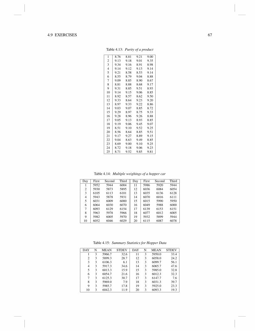
4.9 EXERCISES 67

Table 4.13: Purity of a product

1 8.76 8.81 9.21 9.002 9.13 9.18 9.01 9.353 9.34 9.16 8.91 8.984 9.14 9.12 9.13 9.145 9.21 8.58 8.53 9.146 8.55 8.79 9.04 8.887 9.09 8.85 8.90 8.678 8.81 8.88 8.68 9.179 9.31 8.85 9.51 8.9310 9.14 9.15 9.06 8.8511 8.92 8.57 8.62 9.5012 9.33 8.64 9.23 9.2013 8.97 9.33 9.22 8.8614 9.03 9.07 8.85 8.7215 9.29 8.97 8.75 9.3316 9.28 8.96 9.26 8.8817 9.05 9.13 8.93 8.8518 9.19 9.06 9.45 9.0719 8.51 9.10 9.52 9.2520 8.56 8.64 8.85 9.5121 9.17 9.27 8.89 9.1522 9.04 8.63 9.49 8.8523 8.69 9.00 9.10 9.2524 8.72 9.18 9.06 9.2325 8.71 9.52 9.85 9.81

Table 4.14: Multiple weighings of a hopper car

Day First Second Third Day First Second Third1 5952 5944 6004 11 5986 5920 59442 5930 5873 5895 12 6036 6084 60543 6105 6113 6101 13 6035 6136 61284 5943 5878 5931 14 6070 6016 61115 6031 6009 6000 15 6015 5990 59506 6064 6030 6070 16 6049 5988 60007 6093 6129 6154 17 6139 6153 61518 5963 5978 5966 18 6077 6012 60059 5982 6005 5970 19 5932 5899 5944

10 6052 6046 6029 20 6115 6087 6078

Table 4.15: Summary Statistics for Hopper Data

DAY N MEAN STDEV DAY N MEAN STDEV1 3 5966.7 32.6 11 3 5950.0 33.42 3 5899.3 28.7 12 3 6058.0 24.23 3 6106.3 6.1 13 3 6099.7 56.14 3 5917.3 34.6 14 3 6065.7 47.65 3 6013.3 15.9 15 3 5985.0 32.86 3 6054.7 21.6 16 3 6012.3 32.37 3 6125.3 30.7 17 3 6147.7 7.68 3 5969.0 7.9 18 3 6031.3 39.79 3 5985.7 17.8 19 3 5925.0 23.3

10 3 6042.3 11.9 20 3 6093.3 19.3

68 4. CONTROL CHARTS

Table 4.16: Outside diameter of injection molded bottles

Head HeadSample 1 2 3 4 Sample 1 2 3 4

1 2.01 2.08 2.08 2.04 11 1.99 1.99 2.09 2.112 1.97 2.03 2.09 2.10 12 1.98 2.02 2.03 2.083 2.03 2.09 2.08 2.07 13 1.99 1.98 2.05 2.044 1.96 2.06 2.07 2.11 14 2.01 2.05 2.07 2.085 1.94 2.02 2.06 2.11 15 2.00 2.05 2.06 2.066 2.01 2.03 2.07 2.11 16 2.00 2.00 2.08 2.147 2.00 2.04 2.09 2.06 17 2.01 2.00 2.05 2.158 2.01 2.08 2.09 2.09 18 2.03 2.09 2.11 2.129 2.01 2.00 2.02 2.07 19 1.99 2.10 2.09 2.09

10 2.01 1.96 2.08 2.11 20 2.01 2.01 2.01 2.11

Table 4.17: Summary Statistics for Injection Data

Sample N MEAN STDEV Sample N MEAN STDEV1 4 2.0525 0.0340 11 4 2.0450 0.06402 4 2.0475 0.0602 12 4 2.0275 0.04113 4 2.0675 0.0263 13 4 2.0150 0.03514 4 2.0500 0.0638 14 4 2.0525 0.03105 4 2.0325 0.0718 15 4 2.0425 0.02876 4 2.0550 0.0443 16 4 2.0550 0.06817 4 2.0475 0.0377 17 4 2.0525 0.06858 4 2.0675 0.0386 18 4 2.0875 0.04039 4 2.0250 0.0311 19 4 2.0675 0.0519

10 4 2.0400 0.0678 20 4 2.0350 0.0500

EXERCISE 4.9.18 p and u charts.Construct the p and u charts for Example 4.3.4.

EXERCISE 4.9.19 Clark and Milligan (1994, qe94-389) report the data in Table 4.18 on fillingbarrels of honey that were provided by Dutch Gold Honey for use in making Haagen-Daz specialblend. The goal was to fill the barrels with at least 660 units, but as little more than that as possible.The values reported are the decimal values x for readings that are 660.x units. Construct a meanschart and a dispersion chart and evaluate the results.

EXERCISE 4.9.20 Table 4.19 gives data from van Nuland (1992, qe96-444) and Chao and Cheng(1996) on a DSC apparatus. Construct a means chart and a dispersion chart for these data andevaluate the results.

Table 4.18: Haagen-Daz special blend

Time TimeSample 1 2 3 Sample 1 2 3

1 0 4 2 11 1 2 22 2 4 1 12 2 2 13 2 4 1 13 1 3 24 0 2 2 14 4 2 25 3 0 1 15 4 0 26 4 4 0 16 0 2 17 2 2 3 17 2 2 48 1 4 2 18 0 4 29 0 0 4 19 4 3 1

10 0 0 2

4.9 EXERCISES 69

Table 4.19: Data on a DSC apparatus

Group Observations1 2.2 2.3 2.0 2.12 1.9 2.1 1.8 1.63 1.7 1.8 1.8 1.94 1.5 2.0 1.7 2.05 1.7 2.2 2.2 1.56 2.2 1.5 2.1 1.87 1.8 2.1 1.8 1.98 2.4 1.8 1.9 2.19 2.2 1.9 2.5 2.8

10 1.8 2.6 1.4 2.311 2.4 2.0 1.8 2.112 1.0 1.1 1.4 1.513 2.0 1.4 0.7 0.414 0.9 1.1 1.3 0.715 1.1 0.9 1.0 1.316 1.0 1.6 1.3 0.917 1.7 1.7 1.0 1.018 1.3 1.0 0.9 1.719 1.4 1.0 0.9 1.610 0.9 0.5 0.7 1.521 0.9 1.5 1.8 1.722 1.8 0.9 1.5 0.623 1.2 1.9 2.1 1.724 1.5 1.7 1.5 1.025 1.5 1.0 1.4 1.2

Table 4.20: Automobile Assembly Data

−0.2302 0.9196 1.2809 0.9288 0.0430 0.4074 1.9086 0.10091.1807 −0.1985 0.2714 −0.1458 −0.1269 0.0350 1.5164 1.1236−0.0814 −0.3408 2.1323 0.3683 0.1120 0.3759 −0.2727 0.2610

1.2097 0.3638 1.3688 2.0566 0.5649 0.7998 0.9407 0.34470.8107 0.1849 0.4069 0.2707 0.0701 −0.0498 −0.6768 0.59090.3270 0.3255 0.7791 1.5059 0.4731 1.1318 0.5256 0.8239−0.1833 1.3530 −0.2356 −0.9623 0.8188 −0.0955 −0.3808 0.3889

0.7145 0.2056Read across and then down.

EXERCISE 4.9.21 Table 4.20 gives Radson and Alwan (1996, qe96-171) data from a car assem-bly plant. Laser sensors are used to measure auto dimensions, and these data are a key dimensionfor attaching front wheel components. Proper placement of these components is related to vehiclestability when driving the car. The measurements are deviations relative to the standard given inmillimeters. Give an individuals chart for these data and evaluate the results.

EXERCISE 4.9.21 When constructing a u chart we use the estimatate

λ ≡ ∑ni=1 yi

∑ni=1 `i

rather than more obvious estimate

λ ≡ ∑ni=1 yi/`i

n.

Show thatVar(

λ

)≤ Var

(λ

).

Chapter 5

Prediction from Other Variables

The primary purpose of Statistics is to allow us to make predictions. Indeed, prediction is a primaryaspect of all science and technology. If we turn on a light switch, we do so in anticipation that ourlittle corner of the world will become brighter. When a school looks at the results of a student’scollege preparatory exam, they do so because they believe the results help predict the performanceof the student in college. Turning on a light switch actually causes the world to get brighter, buta college preparatory exam does not cause a student to do well or poorly in school. The collegepreparatory exam is merely correlated with student performance. High exam scores tend to go withgood performance and low exam scores with poor performance — but the relationship is far fromperfect.

The point of control charts is that if a process is under control, we can expect the future behaviorof the process to be like the past behavior that we observed. In this chapter we examine the use of onevariable, such as preparatory exam score, to predict another variable, such as grade point average(gpa) after two semesters. To make such predictions, we will need training data on the exam scoresand 2nd semester gpas for a collection of students. From these data we can develop a predictionmodel and when a new student is presented to us with their exam score, we can predict their 2ndsemester gpa. An important aspect of data based prediction is that the data for the prediction must becollected in a similar fashion to the training data. For example, a predictive model based entirely ondata from suburban high school students will probably not work well for predicting the performanceof inner city high school students.

Not all prediction models are created equally. Although ACT and SAT scores unquestionablyhave some ability to predict 2nd semester gpa, there is a lot of error in such predictions. On the otherhand, if you are rolling a smooth round steel ball over a given smooth surface for exactly 2 seconds,the initial velocity of the ball will be very good at predicting how far the ball will roll. But again,the quality of the predictions depend on having the future observations being taken similarly to thepast observations. If we change the steel ball or the surface on which it is rolling, using the past datato predict these new events is highly questionable.

Statistical analysis cannot properly be used as the basis for inferring causation. Statistical anal-ysis is only concerned with correlation, i.e., the tendency of two events to occur together. We havealready discussed the fact that college preparatory exam scores do not in any reasonable way cause2nd semester gpas. We said that turning on a light switch causes more light, but the causation thatwe infer is not based on statistics. It is based on the idea that turning the switch will complete anelectrical circuit that will cause the light bulb to work. The statistics involved are simply the datathat the switch is turned and the light comes on. It could be that turning on the switch gives anelectrical jolt to a rat who then often decides to eat something and the rat’s food tray is set up so thatthe light goes on when the rat eats something. In this case the rat eating can be considered a cause,but the electrical jolt given the rat is merely correlated with the light coming on — no matter howreliable is the event of the light coming on when the switch is thrown.

71

72 5. PREDICTION FROM OTHER VARIABLES

Table 5.1: Prater’s gasoline–crude oil data

y x y x y x y x6.9 235 10.0 267 24.8 360 32.1 444

14.4 307 15.2 300 26.0 365 34.7 3457.4 212 26.8 367 34.9 395 31.7 4028.5 365 14.0 351 18.2 272 33.6 4108.0 218 14.7 379 23.2 424 30.4 3402.8 235 6.4 275 18.0 428 26.6 3475.0 285 17.6 365 13.1 273 27.8 416

12.2 205 22.3 275 16.1 358 45.7 407

Figure 5.1: Gasoline percentage versus temperature.

5.1 Scatter Plots and Correlation

A scatter plot is a simple tool for seeing whether a relationship exists between two variables and itis even a simple tool for making predictions.

EXAMPLE 5.1.1. Table 5.1 gives data from Hader and Grandage (1958), Atkinson (1985), andChristensen (1996, Exercise 13.8.3.) on y, the percent of gasoline obtained from crude oil,and x, thetemperature in ◦F at which all the crude oil is vaporized. Figure 5.1 is a scatter plot showing therelationship between x and y. From the plot, if the temperature were 325◦F, we would predict about15% gasoline. More realistically, we might predict somewhere between 9% and 24%. Notice thatthe data seem to be more variable as the temperature increases, e.g., the data are more spread outaround 425◦F than they are around 225◦F.

In the next section we will introduce a mathematical model for prediction. The model is going toassume that the variability in the data does not depend on the temperature. Since that is not the casefor these data, we need to do something. A standard method of dealing with this problem is to trytransforming the data. In Figures 5.2, 5.3, and 5.4, we have plotted three standard transformations ofthe data:

√y, log(y), and 1/y versus temperature. In Figure 5.2 the data seem to maintain the same

variability throughout. In Figures 5.3 and 5.4, the data get less variable as temperature increases.From Figure 5.2 we might predict the square root of the gasoline percentage for 325◦F to be

about 4 with an interval of about 2.5 to 5. This corresponds to predictions of 16% with an interval

5.1 SCATTER PLOTS AND CORRELATION 73

Figure 5.2: Square root of gasoline percentage versus temperature.

Figure 5.3: Natural logarithm of gasoline percentage versus temperature.

74 5. PREDICTION FROM OTHER VARIABLES

Figure 5.4: Reciprocal of gasoline percentage versus temperature.

of 9% to 25%. Admittedly, these are very crude and come from simply looking at the picture. Theyare also about what we got from Figure 5.1. For some purposes, these predictions may be entirelyadequate. In the next section, we develop more sophisticated prediction methods.

The correlation coefficient is a unitless number between −1 and 1 that measures the linear rela-tionship between two variables. A value of 0 indicates no linear relationship and values of −1 and1 indicate perfect linear relationships. A value of 1 indicates a perfect positive linear relationship.For example if the correlation between temperature and square root of gasoline percentage was 1,then the plot of the two variables would be a perfect line with a positive slope. The positive slopeindicates that as one variable increases, the other also increases. In Figure 5.2, the data form a linebut it is far from perfect. In particular, the sample correlation is the sample covariance divided bythe product of the sample standard deviations:

r ≡sxy

sxsy= 0.729.

Similarly, a value of −1 indicates a perfect negative linear relationship. If the correlation betweentwo variables is −1, then the plot of the two variables would be a perfect line with a negative slope,so that as one variable gets larger, the other variable gets smaller.

5.2 Simple Linear Regression

What we are seeing in both Figures 5.1 and 5.2 is something that looks basically like a line. However,it is not a perfect linear relationship, so the line must incorporate some error. For n data points, weuse the statistical model

yi = β0 +β1xi + εi (5.2.1)

i = 1, . . . ,n where the line is y = β0 + β1x and the errors εi are assumed to be independent andidentically distributed as N(0,σ2). In this model, yi is an observable random variable and xi istreated as a fixed known number. There are three unknown parameters, β0 and β1 from the line andσ2, the variance of the errors. We estimate β0 and β1 by taking them to minimize

n

∑i=1

(yi−β0−β1xi)2.

5.2 SIMPLE LINEAR REGRESSION 75

Notice that the yis and xis are observed, so only β0 and β1 are unknown. The minimizing values, sayβ0 and β1 are called least squares estimates. It turns out that

β0 = y·− β1 x·; β1 =sxy

s2x.

The variance σ2 is estimated by something call the mean squared error (MSE). The estimated errors(residuals) are

εi ≡ yi−(

β0 + β1xi

)and we average their squared values to get the MSE,

MSE =1

n−2

n

∑i=1

(yi− β0− β1xi)2.

Note that in averaging the squared errors, we divide by n−2 rather than n, that is because to obtainthe estimated errors we had to estimate two parameters β0 and β1. MSE is an unbiased estimate ofσ2, i.e.,

E(MSE) = σ2.

Similarly, it turns out thatE(β0) = β0; E(β1) = β1.

The least squares estimates have

Var(β0) = σ2[

1n+

x2·

(n−1)s2x

]; Var(β1) =

σ2

(n−1)s2x.

Therefore,

SE(β0) =

√MSE

[1n+

x2·

(n−1)s2x

]; SE(β1) =

√MSE

(n−1)s2x.

5.2.1 Basic Analysis

For the gasoline data of Table 5.1, the estimated regression equation is√y =−0.137+0.0132x.

Typically, information about the regression is given by computer programs in two tables:

Table of CoefficientsPredictor βk SE(βk) t PConstant −0.1366 0.7676 −0.18 0.860x 0.013226 0.002263 5.84 0.000

Analysis of VarianceSource df SS MS F pRegression 1 26.386 26.386 34.14 0.000Error 30 23.184 0.773Total 31 49.570

Historically, the place for the Mean Squared Total is left blank but its value would be the samplevariance of all n (here 32) observations in the data, ignoring any and all structure in the data.

The first table gives the estimated regression coefficients β0 = −0.1366 and β1 = 0.013226 inthe second column. The first column simply identifies the terms. The third column gives a measureof variability in the estimate called the standard error. Roughly, we will be 95% confident that the

76 5. PREDICTION FROM OTHER VARIABLES

true value of the parameters is within two standard errors of the estimate. In other words, we areroughly 95% confident that β1 will be somewhere between of−0.1366−2(0.7676) and−0.1366+2(0.7676). The multiplier 2 is what is “rough” about this interval. The multiplier should depend onthe sample size, getting larger for small samples (giving bigger intervals and less precise knowledge)and smaller for large samples. The column t provides tests of whether the regression coefficients β0and β1 are different from 0. The values are computed as t = βk/SE(βk). Roughly, if the value oft corresponding to β1 is larger than 2, there is statistical evidence that β1 6= 0. In simple linearregression, a value of β1 = 0, indicates that there is no relationship between x and y, i.e., the modelbecomes

yi = β0 + εi

which does not involve x. Again, the comparison value of 2 is only rough. It should change with thesamples size. The final column is labeled P and gives information about the t tests. If the parameterbeing tested really does equal 0, P gives the probability of seeing a value of t that is as weird orweirder than what we actually saw. In this context, weird values are those that are far from 0. Afterall, βk is an estimate of βk, so if βk = 0, then βk should be close to 0, relative to its intrinsic variabilitywhich is measured by SE(β1). For testing β1 = 0, having P = 0.000 means that if β1 really is 0, weare seeing something extremely rare. There is almost no chance (P = 0.000) of getting a value oft as large as 5.84 when β1 is 0. If there is a very small chance of seeing a t value this large whenβ1 = 0, it follows logically that β1 is probably not 0. Confidence intervals and tests are discussed inmore detail in the next section.

The second table is called the Analysis of Variance (ANOVA) table. The entry in row “Error”and column “MS” is the mean squared error. The columns are Sources, degrees of freedom (df),sums of squares (SS), mean squares (MS), F , and P. Notice that if we add the degrees of freedomfor Regression and Error we get the degrees of freedom for Total. The same thing works for thesums of squares but not the mean squares. The mean squares are just the sums of squares divided bythe degrees of freedom. The F statistic provides at test of whether β1 = 0 with values much largerthan 1 indicating that β1 6= 0. Roughly, in this context, by much larger than 1 we mean larger than4. Note that

F = 34.14 = (5.84)2

where 5.84 is the t value corresponding to β1. The P value is the same as for the t test of β1 = 0. Inthis context, it is the probability of getting a value of F as large or larger than 34.14 when β1 = 0.

An internal measure of predictive ability of a model is the coefficient of determination

R2 = 53.2% = 0.532.

From the SS column of the Analysis of Variance Table, R2 = 26.386/49.570. It is the percentage ofthe total variability that is being explained by the simple linear regression model. This is an internalmeasure of the predictive ability in that it is based entirely on how the model fits this one set ofdata. An external measure of predictive ability would examine how well this model predicts for adifferent set of data that were collected similarly. R2 values close to 1 indicate very strong predictiveabilities and R2 values close to 0 indicate weak predictive abilities. Note that R2 is not a measureof whether this model is correct or incorrect, it is a measure of how useful the model is for makingpredictions. Note also that if β1 6= 0, the model has some usefulness for making predictions. R2 is ameasure of how much usefulness it has.

It should be noted that in cases like this with only one predictor variable, R2 is the same as thesquare of the correlation coefficient, i.e., R2 = r2.

5.2.2 Residual Analysis

Finally, the model involves assumptions that the εis are independent distributed N(0,σ2). It is im-portant to check these assumptions and we do so by using the residuals

εi = yi−(

β0 + β1xi

).

5.2 SIMPLE LINEAR REGRESSION 77

Figure 5.5: Residuals versus predicted values, data: root y

Actually, we most often use standardized residuals

ri =εi√

MSE(1−hi)

where the term in the denominator is an estimate of the standard deviation of the residual, so isdesigned to make the standardized residual have a variance of about 1. The leverage hi measureshow strange a particular value of xi is relative to the other xis.

The residuals are often plotted against the predicted values (fitted values)

yi = β0 + β1xi.

In this plot we are looking to see an amorphous blob of points. Any systematic structure such asa curve or a horn shape indicates problems with the model. Figure 5.5 gives this plot and it seemsalright.

The residuals are also often plotted against normal scores (rankits). In this plot we are lookingfor something that is roughly a straight line. Strong deviations from a straight line indicate problemswith the normality assumption. The value of R2 between the residuals and the normal scores is calledW , to distinguish it from the R2 between for x and y. Small values of W indicate problems withnormality. W = 0.988 for these data, which is good. The normal scores plot is given as Figure 5.6.A little of the theory behind normal plots is presented in Section 11.4 (in order to motivate methodsfor analyzing data that do not provide a MSE).

5.2.3 Prediction

The prediction of√

y at 325 degrees is

4.162 =−0.137+0.0132(325).

Transforming back to the original scale gives a prediction of 4.1622 = 17.322%. A 95% predic-tion interval is (2.338, 5.985) which transforms back to (5.47, 35.82). In other words, we are 95%

78 5. PREDICTION FROM OTHER VARIABLES

Figure 5.6: Normal Plot for root y; W = 0.988

confident that a new observation at 325 degrees would give a gasoline yield of between 5.47% and35.82%. In an effort to get something in line with the crude intervals of section 1, an 80% predictioninterval is (2.99225,5.33175) which transforms back to (8.95, 28.42), not too far from the values ofSection 1.

Again, the 95% prediction intervals are roughly the prediction plus and minus 2 times an appro-priate standard error. The prediction is an estimate of the point on the line β0 +β1(325). There areactually two different issues of interest relative to this value. One is just to estimate the value and tomeasure how much variability there is in the estimate. The other is to use the estimate as a predictionfor a new observation at 325 degrees and to measure how much variability there is for predictinga new observation. Note that when used for prediction, the variability will be greater because thereis variability associated with using the estimate of the value of the line at 325 degrees plus there isvariability that is intrinsic to taking a new observation.

For these data the standard error for the value of the line at 325 is SE(line) = 0.156. A 95% con-fidence interval for β0 +β1(325) is (3.843,4.481). Note that this is roughly 4.162±2(0.156). Actu-ally, it is roughly 4.162±2.04(0.156). On the original scale this transforms back to (3.8432,4.4812)or (14.77, 20.08).

To get a prediction interval we need

SE(pred.) =√

MSE +SE(line)2 =√

0.773+(0.156)2 = 0.8929.

so the 95% prediction interval is roughly 4.162± 2(0.8929), or is precisely 4.162± 2.04(0.8929),which is (2.338, 5.985). The 80% prediction interval involves changing the multiplier from around2 to 1.31. In particular, the interval is 4.162±1.31(0.8929).

It turns out that for predicting at a point x,

SE(line)2 = MSE[

1n+

(x− x·)2

(n−1)sx2

].

5.3 STATISTICAL TESTS AND CONFIDENCE INTERVALS 79

5.3 Statistical Tests and Confidence Intervals

In statistics, we frequently establish models to help explain the behavior of data. Often we want tocheck whether those models seem reasonable. The purpose of a statistical test is to check whether thedata are consistent with a specified model. The model establishes certain predictions about how datashould behave. We then collect data and check whether the data are consistent with the predictions.In particular, many statistical tests are based on identifying a parameter of interest (Par), an estimate(Est) of that parameter, a measure of the variability of the estimate [SE(Est)], and a distributionfor (Est −Par)/SE(Est). For example, with the data of Example 5.2.1, suppose we hypothesizea simple linear regression model in which the slope parameter β1 equals 0.02. We want to checkwhether the data are consistent with this hypothesized model, or whether the data (tend to) contradictit. If our interest focuses on β1, we have a parameter of interest (Par ≡ β1). We already have anestimate of β1, β1 = 0.013226. If our model with β1 = 0.02 is correct, the estimate β1 should be closeto 0.02. We evaluate this by checking whether 0.013226−0.02 is close to zero. Is 0.013226−0.02is close to zero? That actually depends on the variability associated with the estimate of β1. Ifour model is correct, in repeated sampling (β1− 0.02)/SE(β1) should have a t(dfE) distribution,where dfE = 30 in Example 5.2.1. This is the behavior predicted by the model. We check thisagainst the data actually collected. We actually have collected data that give us β1 = 0.013226 andSE(β1) = 0.002263, so if our model is correct (0.013226−0.02)/0.002263 =−2.99 should be oneobservation from a t(30) distribution. In sampling from a t(30), 99.44% of the time we would getan observation closer to zero than −2.99. Only 0.56% of the time would we get something fartherfrom zero than −2.99. The value −2.99 does not seem like it could reasonably come from a t(30)distribution, as it was supposed to if our model were correct. The data seem to contradict the model.The number 0.56% = 0.0056 given above is called the P value, and is used as a measure of howstrange these data are relative to the behavior predicted by the model.

Sometimes tests are presented as formal decision rules as to whether the model should be re-jected or not. In such cases, an α level is chosen (usually 0.05 or 0.01), and the model is rejectedif P < α . Another way to write this procedure is to find t(1−α/2,dfE), the number that cuts offthe top α/2 of a t(dfE) distribution. For α = 0.05 and dfE = 30, this is t(0.975,30) = 2.0423. Theformal decision rule is to reject the model if

Est−0.02SE(Est)

=β1− .02

SE(β1)> 2.0423

of ifEst−0.02SE(Est)

=β1− .02

SE(β1)<−2.0423.

Note that the decision rule can be established without knowing the data — but using the rule requiresknowing actual values for β1 and SE(β1).

This test has been focused on a particular parameter of the model, β1. While the test is reallya test of whether the entire model fits, it is particularly good at detecting differences β1 6= 0.02. Infact, the test is often presented as a test of a null hypothesis H0 : β1 = 0.02 versus an alternativehypothesis HA : β1 6= 0.02. But this formulation ignores the sensitivity of the test to all of the aspectsof the model other than β1 = 0.02.

A 95% confidence interval for β1 contains all of the parameter values β1 that are consistent withthe data (and the model) as evaluated by an α = 0.05 test. Here, 95% = 0.95 = 1− .05 = 1−α . The95% confidence interval is every parameter value β1 that cannot be rejected in an α = 0.05 test. Aparticular value β1 will not be rejected if

−t(1−α/2,dfE)<β1−β1

SE(β1)< t(1−α/2,dfE) .

80 5. PREDICTION FROM OTHER VARIABLES

Table 5.2: Prater’s gasoline–crude oil data

y x1 x2 x3 x4 y x1 x2 x3 x46.9 38.4 6.1 220 235 24.8 32.2 5.2 236 360

14.4 40.3 4.8 231 307 26.0 38.4 6.1 220 3657.4 40.0 6.1 217 212 34.9 40.3 4.8 231 3958.5 31.8 0.2 316 365 18.2 40.0 6.1 217 2728.0 40.8 3.5 210 218 23.2 32.2 2.4 284 4242.8 41.3 1.8 267 235 18.0 31.8 0.2 316 4285.0 38.1 1.2 274 285 13.1 40.8 3.5 210 273

12.2 50.8 8.6 190 205 16.1 41.3 1.8 267 35810.0 32.2 5.2 236 267 32.1 38.1 1.2 274 44415.2 38.4 6.1 220 300 34.7 50.8 8.6 190 34526.8 40.3 4.8 231 367 31.7 32.2 5.2 236 40214.0 32.2 2.4 284 351 33.6 38.4 6.1 220 41014.7 31.8 0.2 316 379 30.4 40.0 6.1 217 3406.4 41.3 1.8 267 275 26.6 40.8 3.5 210 347

17.6 38.1 1.2 274 365 27.8 41.3 1.8 267 41622.3 50.8 8.6 190 275 45.7 50.8 8.6 190 407

Some algebra establishes that β1 will satisfy these conditions if and only if

β1− t(1−α/2,dfE)SE(β1)< β1 < β1 + t(1−α/2,dfE)SE(β1).

The endpoints of the interval are

β1± t(1−α/2,dfE)SE(β1).

For our data with dfE = 30 and α = 0.05, this is 0.013266± 2.0423(0.002263) for an interval(0.00864, 0.01789).

In more generality, if you have a Par of interest, with Est and SE(Est), and the distribution(Est−Par)/SE(Est)∼ t(dfE), then a, say, 99% confidence interval will have limits

Est± t(1−α/2,dfE)SE(Est),

where α = 1−0.99.

5.4 Scatterplot Matrix

It is relatively easy to see the relationship between two variables simply by plotting them. Witha sophisticated plotting device, one can even examine the relationships between three variables,however with more than three variables, simultaneous plotting becomes impossible. One commonlyused method to overcome this is the scatterplot matrix. It is simply a matrix of all of the pairwiseplots that can be constructed from a collection of variables,

EXAMPLE 5.4.1. Hader and Grandage (1958), Atkinson (1985), and Christensen (1996) havepresented Prater’s data on gasoline. The variables are y, the percentage of gasoline obtained fromcrude oil; x1, the crude oil specific gravity oAPI; x2, crude oil vapor pressure measured in lbs/in2;x3, the temperature in oF at which 10% of the crude oil is vaporized; and x4, the temperature in oFat which all of the crude oil is vaporized. The data are given in Table 5.2. Ideally, a scatterplot matrixwould be a 5× 5 array of plots but that it too big to fit well on a page. A scatterplot matrix of thepredictor variables x j is given in Figure 5.7 and Figure 5.8 contains plots of y versus the predictorvariables.

In Section 1 we examined the simple linear regression between√

y and what we are now callingx4.√

y was used in that example because if you look at a plot of y on x4, (or a plot of the residuals

5.4 SCATTERPLOT MATRIX 81

Figure 5.7: Scatterplot Matrix for Gasoline Data: Predictor variables.

Figure 5.8: Scatterplot Matrix for Gasoline Data: Predictor variables with y.

82 5. PREDICTION FROM OTHER VARIABLES

versus x4), the variability of y seems to increase with the value of x4. Note that this plot also occurson the right side of Figure 5.8. A log transformation did not seem to eliminate the problem, but thesquare root seemed to work fine. Alas, the situation is somewhat more complex. If you look at theplot of x3 versus x4, you see a rough linear trend in which the x3 values show increased variability asx4 increases. However, x3 is also an important predictor of y that we were ignoring in Section 1. Inthe simple linear regression of y on x4, the increasing variability is really a lack of fit. By ignoringthe important variable x3, we expect to see more variability. If the x3 values are more spread out forlarge x4 values than for small x4 values, we should fit the line worse at large x4 values than at smallones. That is exactly what we saw. It turns out that if you do a regression of y on both x3 and x4, youdo not see the same serious problem with residual variability.

5.5 Multiple Regression

We now want to extend the ideas of simple linear regression to include all 4 of the predictor variablesincluded in the Prater data. A multiple regression model is

yi = β0 +β1xi1 +β2xi2 +β3xi3 +β4xi4 + εi, i = 1, . . . ,32 .

In general, with n observations and p predictor variables the model is

yi = β0 +β1xi1 +β2xi2 + · · ·+βpxi,p + εi, i = 1, . . . ,n , (5.5.1)

where εis are assumed to be independent N(0,σ2).

EXAMPLE 5.5.1. For the Prater data we examine a regression of y on x1, x2, x3, and x4:

yi = β0 +β1xi1 +β2xi2 +β3xi3 +β4xi4 + εi . (5.5.2)

The estimated regression equation is

y =−6.8+0.227x1 +0.554x2−0.150x3 +0.155x4

with tables of statisticsTable of Coefficients

Predictor Est SE t PConstant −6.82 10.12 −0.67 0.506x1 0.22725 0.09994 2.27 0.031x2 0.5537 0.3698 1.50 0.146x3 −0.14954 0.02923 −5.12 0.000x4 0.154650 0.006446 23.99 0.000

Analysis of VarianceSource df SS MS F PRegression 4 3429.27 857.32 171.71 0.000Error 27 134.80 4.99Total 31 3564.08

In the coefficients table, we have the least squares (maxium likelihood) estimates of each param-eter, the standard error of each parameter, the t statistic for testing whether the coefficient is equalto 0, and the P value for the test. Note that for x3 the t statistic is−5.12 which is far from 0 and veryinconsistent with β3 being equal to 0, as measured by the very small P value. Thus it is clear thatx3 is needed to help explain the data. On the other hand, there is no strong evidence that β2 6= 0 andthe evidence that β1 6= 0 is much weaker than for β3 and β4. So there is no strong evidence that x2is needed in the model and relatively weak evidence that x1 is needed. A key fact about this table is

5.5 MULTIPLE REGRESSION 83

that everything depends on everything else. For example, if we decided that a variable should onlybe in the model if the corresponding P value is less than 0.01, we could conclude that either x1 orx2 can be dropped from the model. But we cannot conclude that both should be dropped from themodel. The test for whether β2 = 0 is based on having x1 in the model and similarly the test forwhether β1 = 0 is based on having x2 in the model. If you want to find out whether you can dropboth x1 and x2 you have to fit a model that drops both variables and compare it to a model that hasall 4 variables. A method for making such comparisons will be discussed later.

In the ANOVA table, the regression has 4 degrees of freedom because there are 4 predictorvariables. The degrees of freedom for error is 27 = 32− 5 where the n = 32 is the number ofobservations in the data and p+1 = 5 is the number of βk coefficients being fitted in the model. Thedegrees of freedom total is n−1 = 32−1 = 31 and the sum of squares total is 31 times the samplevariance of the 32 y values. The sum of squares error is the sum of squared residuals. The residualsare

εi = yi− β0− β1xi1− β2xi2− β3xi3− β4xi4

and

SSE =n

∑i=1

ε2i =

n

∑i=1

(yi− β0− β1xi1− β2xi2− β3xi3− β4xi4)2.

The mean squared error is

MSE = SSE/dfE = 134.80/27 = 4.99.

The sum of squares regression is the sum of squares total minus the sum of squares error,

SSReg = 3564.08−134.80 = 3429.27

The F statistic provides a test of whether any of the predictor variables is useful in explaining thedata, i.e., it tests whether we could drop all of x1, x2, x3, and x4 and still do an adequate job ofexplaining the data, i.e., it tests whether β1 = β2 = β3 = β4 = 0. The test is rejected if the F valueis much larger than 1. In particular, the test is rejected if, assuming the variables are not needed, theprobability of seeing an F value as large or larger than the one we actually saw is too small, i.e., ifthe P value is too close to 0.

The R2 for these data is

R2 =SSRegSSTot

=3429.273564.08

= 96.2%.

Consider a prediction for the values x1 = 44, x2 = 6, x3 = 230, x4 = 230. Using the estimatedregression equation, the point prediction is

7.677 =−6.8+0.227(44)+0.554(6)−0.150(230)+0.155(230) .

Typical computer output provides a standard error for the fitted surface, in this example it isSE(sur f ) = 0.953. As discussed in Section 2, this standard error must be modified to give a standarderror appropriate for a prediction interval,

SE(pred) =√

MSE +[SE(sur f )]2 =√

4.99+[0.953]2) = 2.429

The 95% prediction interval is approximately 7.677 plus or minus 2 times this standard error. Herethe exact interval involves a multiplier slightly larger than 2, so the exact interval is (2.692,12.662),cf. Christensen (1996, Secs. 13.2 and 15.4).

The sequential sums of squares areSource df Seq SS

x1 1 216.26x2 1 309.85x3 1 29.21x4 1 2873.95

84 5. PREDICTION FROM OTHER VARIABLES

5.6 Polynomial Regression

We can fit more general models than those used in the previous section. In particular we can use thesame methods for fitting quadratic models. For simplicity, we focus on only two variables. For thePrater data we focus on x3 and x4. We now consider a quadratic model

yi = β00 +β10xi3 +β01xi4 +β20x2i3 +β02x2

i4 +β11xi3xi4 + εi .

The fitted regression equation is

y = 40.6−0.371x3 +0.133x4 +0.000687x23 +0.000222x2

4−0.000519x3x4.

The tables of statistics are similar to those used earlier.

Table of CoefficientsPredictor Est SE t PConstant 40.59 19.78 2.05 0.050x3 −0.3712 0.1462 −2.54 0.017x4 0.13330 0.06214 2.15 0.041x2

3 0.0006872 0.0003288 2.09 0.047x2

4 0.0002224 0.0001114 2.00 0.056x3x4 −0.0005187 0.0002380 −2.18 0.039

Analysis of VarianceSource df SS MS F PRegression 5 3431.38 686.28 134.46 0.000Error 26 132.70 5.10Total 31 3564.08

R2 = 96.3%

In addition, one should examine residual plots and one can examine predictions.Figures 5.9 and 5.10 plot the regression surface. In experimental design such polynomial sur-

faces are referred to as response surfaces and are the subject of considerable theory, cf TiD.

5.7 Matrices

Computations and theory for regression are greatly simplified by using matrices. Virtually all com-puter programs for doing regression are matrix oriented. We briefly introduce matrix notation forregression problems. This section presumes that the reader knows how to add and multiply matrices.Near the end we also use the concepts of the transpose of a matrix and of the inverse of a squarematrix. A vector is a matrix with just one column.

EXAMPLE 5.7.2. Simple Linear Regression.Consider the relationship between y, the percent of gasoline obtained from crude oil, and x, thetemperature in ◦F at which all the crude oil is vaporized. Five observations are given below.

xi yi307 14.4365 26.0235 2.8428 18.0345 34.7

We can fit the modelyi = β0 +β1xi + εi, i = 1, . . . ,5,

5.7 MATRICES 85

Figure 5.9: Surface plot of y.

Figure 5.10: Contour plot of y.

86 5. PREDICTION FROM OTHER VARIABLES

where the εi’s are assumed to be independent N(0,σ2). In matrix notation we can write the modelas

y1y2y3y4y5

=

β0 +β1(307)+ ε1β0 +β1(365)+ ε2β0 +β1(236)+ ε3β0 +β1(428)+ ε4β0 +β1(345)+ ε5

. (5.7.1)

These two matrices are equal if and only if the corresponding elements are equal, which occursif and only if the simple linear regression model holds. The xi’s are assumed to be fixed knownnumbers, so we have incorporated them into the statement of the model. The yi’s are assumed to berandom variables, the values given earlier for the yi’s are realizations of the random variables. Weuse them to fit the model (estimate parameters), but they are not part of the model itself.

We can also write the simple linear regression model asy1y2y3y4y5

=

1 3071 3651 2351 4281 345

[

β0β1

]+

ε1ε2ε3ε4ε5

Y = X β + e

Multiplying and adding the matrices on the right-hand side establishes that this is equivalent toequation (5.7.1). Note that we observe the Y vector to be

Y = (14.4,26.0,2.8,18.0,34.7)′.

In general, the model yi = β0 +β1xi + εi, i = 1, . . . ,n, can be written asy1y2...

yn

=

β0 +β1x1 + ε1β0 +β1x2 + ε2

...β0 +β1xn + εn

or, equivalently,

y1y2...

yn

=

1 x11 x2...

...1 xn

[β0β1

]+

ε1ε2...

εn

Yn×1 = Xn×2 β2×1 + en×1

The usual conditions are that the εi’s are independent N(0,σ2). We can restate this as that (a) allεis are independent, (b) E(εi) = 0 for all i, (c) Var(εi) = σ2 for all i, (d) all are normally distributed.Condition (b) translates into matrix terms as

E(e)≡

E(ε1)E(ε2)

...E(εn)

=

00...0

= 0n×1,

where 0 is the n×1 matrix containing all zeros. Conditions (a) and (c) imply that

Cov(e) = σ2I,

5.7 MATRICES 87

where I is the n× n identity matrix. Here Cov(e) is defined as the n× n matrix with i j elementCov(εi,ε j). By definition, the covariance matrix Cov(e) has the variances of the εi’s down the di-agonal. The variance of each individual εi is σ2, so all the diagonal elements of Cov(e) are σ2, justas in σ2I. Also by definition, the covariance matrix Cov(e) has the covariances of distinct εi’s as itsoff-diagonal elements. The covariances of distinct εi’s are all 0 because they are independent, so allthe off-diagonal elements of Cov(e) are zero, just as in σ2I.

In general linear model is any model

Y = Xβ + e,

where Y is an observable random vector, X is fixed and known, β is fixed but unknown, so e is theonly thing random on the right of the equation and E(e) = 0. It follows that

E(Y ) = E(Xβ + e) = Xβ +E(e) = Xβ

and, with our usual assumptions about the εis,

Cov(Y ) = Cov(Xβ + e) = Cov(e) = σ2I.

These results follow directly from properties enumerated in Subsection 3.3.3 but, more to the point,they are intuitive since the vector Xβ is fixed and has no variability. Cov(e) = σ2I is a common butnot necessary assumption for having a linear model.

EXAMPLE 5.7.3. Polynomial Regression.Rather than fitting a line to the (x,y) data of Example 5.7.2, we can fit, say, a quadratic model,

yi = β0 +β1xi +β2x2i + εi, i = 1, . . . ,5,

where the εi’s are assumed to be independent N(0,σ2). In matrix notation we can write the modelas

y1y2y3y4y5

=

β0 +β1(307)+β2(3072)+ ε1β0 +β1(365)+β2(3652)+ ε2β0 +β1(236)+β2(2362)+ ε3β0 +β1(428)+β2(4282)+ ε4β0 +β1(345)+β2(3452)+ ε5

.or

y1y2y3y4y5

=

1 307 3072

1 365 3652

1 235 2362

1 428 4282

1 345 3452

β0

β1β2

+

ε1ε2ε3ε4ε5

Y = X β + e.

In general, the model yi = β0 +β1xi +β2x2i + εi, i = 1, . . . ,n can be written as

y1y2...

yn

=

β0 +β1x1 +β2x2

1 + ε1β0 +β1x2 +β2x2

2 + ε2...

β0 +β1xn +β2x2n + εn

or, equivalently, as

y1y2...

yn

=

1 x1 x2

11 x2 x2

2...

......

1 xn x2n

β0

β1β2

+

ε1ε2...

εn

88 5. PREDICTION FROM OTHER VARIABLES

Similarly, the cubic model yi = β0 +β1xi +β2x2i +β3x3

i + εi, i = 1, . . . ,n, can be written as

y1y2...

yn

=

β0 +β1x1 +β2x2

1 +β3x31 + ε1

β0 +β1x2 +β2x22 +β3x3

2 + ε2...

β0 +β1xn +β2x2n +β3x3

n + εn

or, equivalently, as

y1y2...

yn

=

1 x1 x2

1 x31

1 x2 x22 x3

2...

......

...1 xn x2

n x3n

β0β1β2β3

+

ε1ε2...

εn

Yn×1 = Xn×4 β4×1 + en×1

Other polynomials follow the same pattern.

EXAMPLE 5.7.5. Multiple Regression.Consider the relationship between y, the percent of gasoline obtained from crude oil, x1, the tem-perature in ◦F at which 10% of the crude oil is vaporized, and x2, the temperature at which all thecrude oil is vaporized. Five observations are given below.

xi1 xi2 yi231 307 14.4220 365 26.0267 235 2.8316 428 18.0190 345 34.7

The multiple regression model can be written as

yi = β0 +β1xi1 +β2xi2 + εi, i = 1,2,3,4,5.

In matrix terms the model can be rewritten as the equality of two 5×1 matrices,y1y2y3y4y5

=

β0 +β1(231)+β2(307)+ ε1β0 +β1(220)+β2(365)+ ε2β0 +β1(267)+β2(235)+ ε3β0 +β1(316)+β2(428)+ ε4β0 +β1(190)+β2(345)+ ε5

.Breaking up the right-hand-side gives

y1y2y3y4y5

=

1 231 3071 220 3651 267 2351 316 4281 190 345

β0

β1β2

+

ε1ε2ε3ε4ε5

Yn×1 = Xn×p βp×1 + en×1.

We could also fit a polynomial in these two variables, say,

yi = β0 +β1xi1 +β2xi2 +β11x2i1 +β22x2

i2 +β12xi1xi2 + εi .

5.7 MATRICES 89

In matrix form this isy1y2y3y4y5

=

1 231 307 2312 3072 231(307)1 220 365 2202 3652 220(365)1 267 235 2672 2352 267(235)1 316 428 3162 4282 316(428)1 190 345 1902 3452 190(345)

β0β1β2β11β22β12

+

ε1ε2ε3ε4ε5

.

The general multiple regression model can be written as

yi = β0 +β1xi1 +β2xi2 + · · ·+βp−1xi,p−1 + εi, i = 1, . . . ,n.

In matrix terms the model involves equality of two n×1 matrices,y1y2...

yn

=

β0 +β1x11 +β2x12 + · · ·+βp−1x1,p−1 + ε1β0 +β1x21 +β2x22 + · · ·+βp−1x2,p−1 + ε2

...β0 +β1xn1 +β2xn2 + · · ·+βp−1xn,p−1 + εn

.Breaking up the right-hand-side gives

y1y2...

yn

=

1 x11 x12 · · · x1,p−11 x21 x22 · · · x2,p−1...

......

. . ....

1 xn1 xn2 · · · xn,p−1

β0β1β2...

βp−1

+

ε1ε2...

εn

Yn×1 = Xn×p βp×1 + en×1

Multiplying and adding the right-hand side gives the equivalence.Once again, the usual conditions on the εi’s translate into

E(e) = 0,

where 0 is the n×1 matrix consisting of all zeros, and

Cov(e) = σ2I,

where I is the n×n identity matrix.For a general linear model

Y = Xβ + e, E(e) = 0, Cov(e) = σ2I,

it is not too difficult to show that the least squares estimates satisfy

β = (X ′X)−1X ′Y,

where X ′ denotes the transpose of the matrix X and, when such a matrix exists, (X ′X)−1 is theunique matrix that satisfies (X ′X)−1(X ′X) = I. The sum of squares for error is

SSE ≡ (Y −X β )′(Y −X β ).

The variances of the β js are the diagonal elements of the matrix

Cov(β ) = σ2(X ′X)−1.

The last three displayed matrix equations are enough to determine both the Table of Coefficientsand the ANOVA table.

90 5. PREDICTION FROM OTHER VARIABLES

Table 5.3: Regression

Output Rate Align B gap Proll Air Temp. Calrd1.83 68 2 1 0.95 2 2 2−3.17 76 1 1 1.05 2 2 1−3.92 68 1 2 0.95 2 1 1

0.83 76 2 1 0.95 1 2 2−3.92 76 1 2 0.95 1 1 1−2.08 85 1 2 1.05 1 2 2−3.08 85 2 2 1.05 2 1 1−4.17 68 2 2 1.05 1 2 1

1.50 76 2 2 1.05 2 1 2−1.58 85 1 1 0.95 2 2 2−3.83 85 2 1 0.95 1 1 1

1.50 68 1 1 1.05 1 1 2

5.8 Logistic Regression

Test for lack of fit of intercept only in any binomial problem from Chapter 4. Test for linear timetrend.

Table 4.18: Haagen-Daz special blend. One-way and Two way. Poisson model?

5.9 Missing Data

Hand, David J. Dark DataMissing at random. Remaining data are still a random sample.Missing because of data you have. (x,y) plot, not allowed to collect y if x is too low. Don’t

complete items that are unlikely to meet specs.Missing because of the data you would have got. (x,y) plot, items with low y not measured. Toss

out items that look like they will not meet specs.

5.10 Exercises

Carter qe96-502Rate: 68 or 76Alignment: right 1 inch (2) or left 1 inch (1)B gap: loose (2) or tight (1)Proll: 0.95 or 1.05Air: closed (2) or open (1)Room Temp.: hot (2) or cold (1)Calrd: on (2) or off (1)

5.10 EXERCISES 91

Table 5.4: DBP Measurements of Carbon Black

Time At Smoke End(Hour) Header Product

7 94.8 90.59 94.8 91.111 94.2 89.113 94.4 89.215 93.4 89.317 94.2 89.219 94.6 87.321 96.6 88.223 96.3 89.71 96.6 91.13 96.7 90.6

Schneider and Pruett (1994). qe94-345predict end product dbp from earlier smoke header dbp.Plot versus lags 0, 1, 2, 3. (lag 1 means 2 hours) get decent correlation at lag 3 but looks weird

in plot. relationship is all from last 3 points with much larger smoke headers.

92 5. PREDICTION FROM OTHER VARIABLES

Table 5.5: Relation between two variables

Bending BendingCase Strength Sturdiness Case Strength Sturdiness

1 170 111 11 171 1132 168 106 12 160 1053 154 108 13 161 1154 170 115 14 160 1075 161 114 15 166 1176 173 113 16 166 1117 172 112 17 171 1088 175 114 18 162 1039 164 109 19 157 106

10 160 106 20 159 107

Shi and Lu(1994). qe94-526 SLR

Chapter 6

Time Series

In an industrial or service process, as discussed in Chapter 4, our ideal is that data generated by theprocess be independent and identically distributed. In particular, the data would all have the samemean value and variance. Processes that display these characteristics are under control. The object ofthis desire for having processes under control is that, when the data are independent and identicallydistributed, we can make predictions about the future of the process. If the process displays changesin the mean value, or the variance, or even in the distribution, often the causes of such changescan be identified and eliminated and the process put back under control. Alas, sometimes (perhapsoften) the problem with a process is that the observations are not independent. Means charts aresensitive to this problem, i.e., they will tend to go out of control more often if the observations havepositive correlation. But lack of independence is typically more difficult to rectify than are problemswith changing means or variances. Fortunately, lack of independence is often a problem that onecan simply live with. Rather than requiring that observations be independent, we can require thatthe observations be stationary.

A sequence of observations is called stationary if the statistical properties of the observationsremain the same regardless of what time you choose to look at them. The word “stationary” isa reference to the fact that these properties do not change. If you have a stationary process, themean values remain the same over time and the variances remain the same over time, just like theywould if the observations were independent and identically distributied. Really, the only assumptionthat is being weakened with stationary observations is the assumption of independence. The beautyof having a stationary process is that one can still make predictions about the future, because theconditions in the future should be the same as those in the past when we collected our data. As amatter of fact, a formal definition of a stationary process includes observations that are independentand identically distributed as a special case of a stationary process. So the methods of Chapter 4 aremethods for a special case of stationary processes.

We need two things to work with stationary processes. First, we need to be able to identify sit-uations in which observations are stationary but not independent. Second, we need to have controlcharts for stationary processes. The next section deals with methods for detecting lack of indepen-dence.

EXERCISE 6.0.1. Watch the video of George Box rethinking quality control and be prepared toanswer very simple questions about it. (You can skip the 15 minutes of Q&A.) He discusses sta-tionary processes, EWMAs, and suggests control charting the estimated errors (residuals) of modelslike those discussed below. He has some attitudes that are very different from Shewhart/Deming inthat at one points he essentially advocates plotting against limits that the process owner would finddisturbingly off target rather than worrying about whether the process is under control. Recall thatEWMA charts are really tests for being on target. Along these lines, the posted comments surround-ing the video provide some perspective. Insightful people tend to do better statistics than dogmaticpeople, no matter how good the dogma is. (And there are some very good statistical dogmas.)

Box quite famously believes that all models are wrong but that some are useful. Not surprisingly,he believes that no real processes are stationary. That brings us back to the issue of finding an

93

94 6. TIME SERIES

Table 6.1: Temperature Data

0.64 0.94 0.91 0.92 0.89 1.04 1.07 0.99 0.95 1.051.14 1.36 1.15 1.25 1.33 1.39 1.35 1.41 1.04 0.931.05 1.53 1.88 1.80 1.65 2.05 2.33 1.72 1.48 1.661.28 0.93 0.87 1.05 1.18 0.86 1.16 1.21 1.22 1.691.59 1.69 0.93 0.57 1.03 1.54 0.98 0.84 0.78 1.031.05 1.31 1.46 1.56 0.91 1.16 1.02 0.80 1.38 1.701.88 2.24 2.03 2.00 2.32 1.59 1.03 1.46 1.93 1.571.20 0.82 1.39 1.32 1.52 1.08 1.16 1.41 1.09 0.89

Read across then down.

Figure 6.1: Plot of temperature data versus time

operational definition of when a process is close enough to being stationary that we can make usefulpredictions.

6.1 Autocorrelation and Autoregression

The next example illustrates a technique from time series analysis for detecting lack of independencein a series of observations.

EXAMPLE 6.1.1 The data in Table 6.1 are from Box and Lucero (1997). They consist of 80temperatures taken “from the output of an industrial process.” Figure 6.1 presents the standardtime series plot of the data versus the time at which the observations were obtained. Since we areinterested in industrial statistics, Figure 6.2 presents the corresponding individuals control chart.The process is wildly out of control. Not only do observations get outside the control limits butMinitab’s supplemental tests 2 and 6 are violated many times and test 8 is also violated. Despite thisfact, one can make a decent case for these data being the result of a stationary process and thereforepredictable and capable of yielding temperatures that could be within some specifications.

Figure 6.3 plots each value against the previous measurement, i.e., it plots the pairs (yt ,yt−1).There is an obvious linear relationship, leading us to expect that the current temperature should giveus some ability to predict the next temperature.

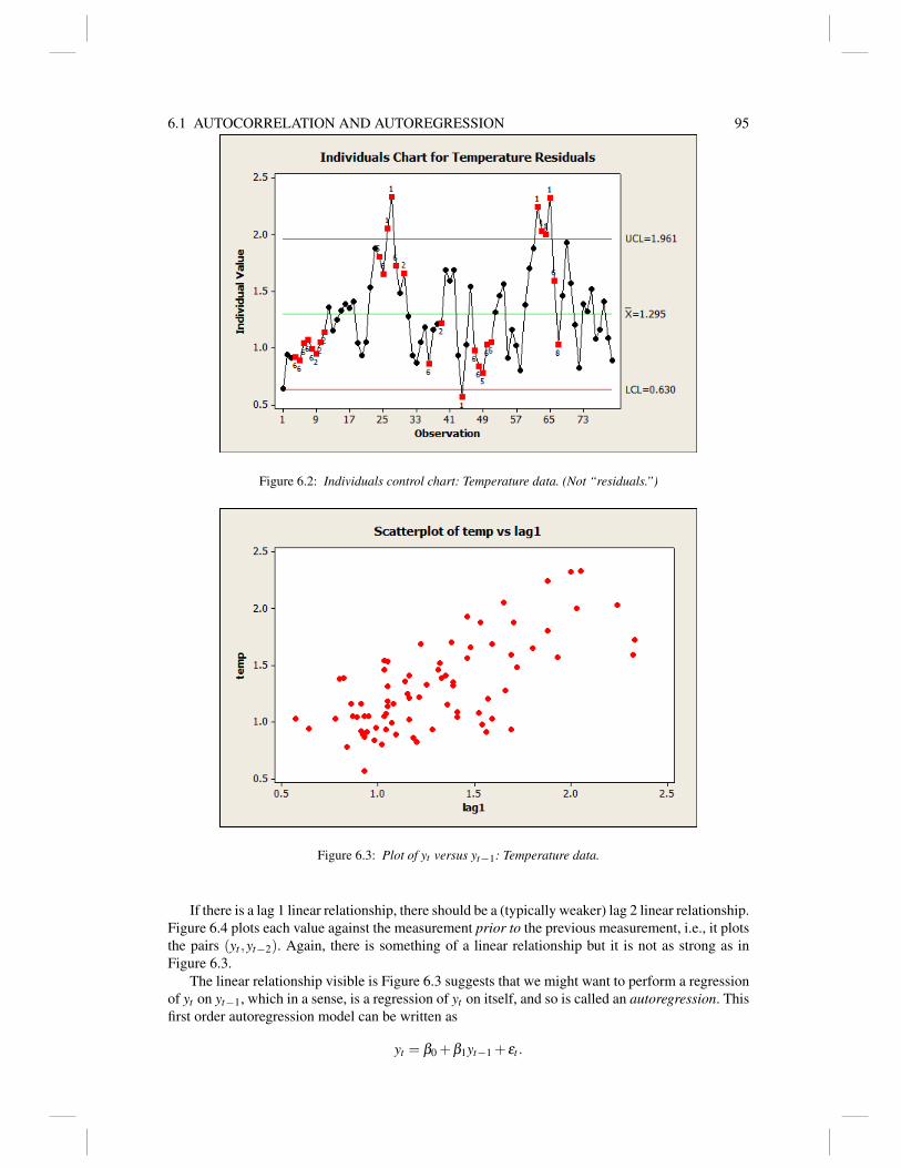
6.1 AUTOCORRELATION AND AUTOREGRESSION 95

Figure 6.2: Individuals control chart: Temperature data. (Not “residuals.”)

Figure 6.3: Plot of yt versus yt−1: Temperature data.

If there is a lag 1 linear relationship, there should be a (typically weaker) lag 2 linear relationship.Figure 6.4 plots each value against the measurement prior to the previous measurement, i.e., it plotsthe pairs (yt ,yt−2). Again, there is something of a linear relationship but it is not as strong as inFigure 6.3.

The linear relationship visible is Figure 6.3 suggests that we might want to perform a regressionof yt on yt−1, which in a sense, is a regression of yt on itself, and so is called an autoregression. Thisfirst order autoregression model can be written as

yt = β0 +β1yt−1 + εt .

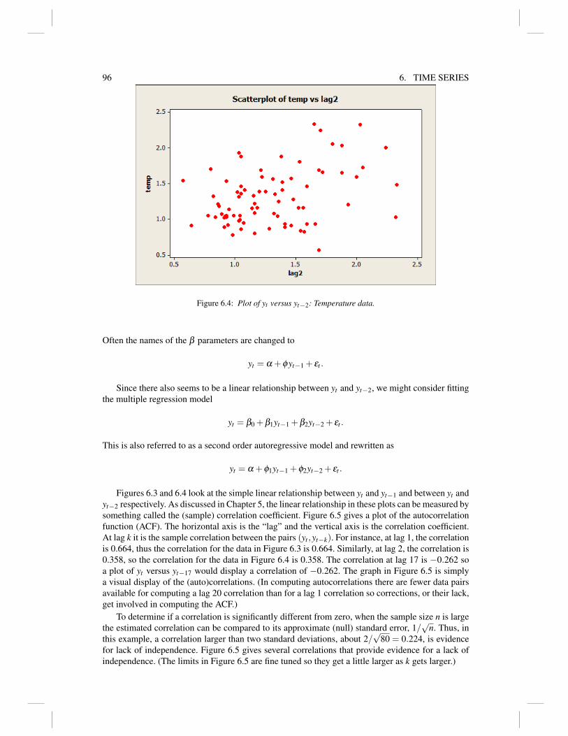
96 6. TIME SERIES

Figure 6.4: Plot of yt versus yt−2: Temperature data.

Often the names of the β parameters are changed to

yt = α +φyt−1 + εt .

Since there also seems to be a linear relationship between yt and yt−2, we might consider fittingthe multiple regression model

yt = β0 +β1yt−1 +β2yt−2 + εt .

This is also referred to as a second order autoregressive model and rewritten as

yt = α +φ1yt−1 +φ2yt−2 + εt .

Figures 6.3 and 6.4 look at the simple linear relationship between yt and yt−1 and between yt andyt−2 respectively. As discussed in Chapter 5, the linear relationship in these plots can be measured bysomething called the (sample) correlation coefficient. Figure 6.5 gives a plot of the autocorrelationfunction (ACF). The horizontal axis is the “lag” and the vertical axis is the correlation coefficient.At lag k it is the sample correlation between the pairs (yt ,yt−k). For instance, at lag 1, the correlationis 0.664, thus the correlation for the data in Figure 6.3 is 0.664. Similarly, at lag 2, the correlation is0.358, so the correlation for the data in Figure 6.4 is 0.358. The correlation at lag 17 is −0.262 soa plot of yt versus yt−17 would display a correlation of −0.262. The graph in Figure 6.5 is simplya visual display of the (auto)correlations. (In computing autocorrelations there are fewer data pairsavailable for computing a lag 20 correlation than for a lag 1 correlation so corrections, or their lack,get involved in computing the ACF.)

To determine if a correlation is significantly different from zero, when the sample size n is largethe estimated correlation can be compared to its approximate (null) standard error, 1/

√n. Thus, in

this example, a correlation larger than two standard deviations, about 2/√

80 = 0.224, is evidencefor lack of independence. Figure 6.5 gives several correlations that provide evidence for a lack ofindependence. (The limits in Figure 6.5 are fine tuned so they get a little larger as k gets larger.)

6.2 AUTOREGRESSION AND PARTIAL AUTOCORRELATION 97

Figure 6.5: Autocorrelation Function for Temperature Data

6.2 Autoregression and Partial Autocorrelation

Earlier we discussed that based on Figures 6.3 and 6.4 we might consider fitting either of the regres-sion models

yt = β0 +β1yt−1 + εt

oryt = β0 +β1yt−1 +β2yt−2 + εt .

The partial autocorrelation function (PACF) displayed in Figure 6.5 can help us decide betweenthe two models. At lag 1, the value in the PACF is identical to the value in the ACF, it is just thecorrelation between yt and yt−1. However, the value of the PACF at lag 2 is very different from thevalue of the ACF at lag 2. At lag 2 the ACF is just the correlation between yt and yt−2. At lag 2 thePACF is the correlation between the residuals from fitting yt on yt−1 and the residuals from fittingyt−2 on yt−1. The idea is that if yt−2 really is needed in the regression model, then there should bea substantial correlation between these two sets of residuals. If there is no such correlation betweenthe residuals, it suggests that the linear relationship we are seeing in Figure 6.4 is merely an artifact.From Figure 6.3, we know that yt and yt−1 are linearly related, which immediately implies that yt−1and yt−2 are linearly related, it follows that there must be some linear relationship between yt andyt−2. The PACF at lag 2 is looking to see if there is any direct relationship between yt and yt−2 overand above the artifactual one induced by them both being related to yt−1. In fact, the correlation of−0.150 is quite small, so there is no evidence that we need to include yt−2 as a predictor variable inour regression.

In general, the lag k partial autocorrelation is the the sample correlation between the residualsfrom regressing yt on yt−1, . . . ,yt−k+1 and the residuals from regressing yt−k on yt−1, . . . ,yt−k+1.

A curious behavior in the PACF for these data is the relatively large value at lag 20 of −0.325.This is indicting that if we regressed yt on all of yt−1, . . . ,yt−19 and regressed yt−20 on all ofyt−1, . . . ,yt−19, the residuals have a correlation of −0.325. This could either be caused by a realphenomenon or could be a mere artifact of the data. If, for example, there were 20 temperaturemeasurements made each day, large PACF values at only lags 1 and 20 indicate that the current tem-perature depends directly on two things, the previous temperature and the temperature at the same

98 6. TIME SERIES

Figure 6.6: Partial Autocorrelation Function for Temperature Data

time the previous day. Such effects on a time series that stem from periods that are far removedare called seasonal effects. The terminology comes from the fact that many business and economictime series display regular changes associated with the seasons of the year. (Retail sales go up everyChristmas, fuel oil sales for heating go down in the summer and up in the winter, etc.) We will notdiscuss seasonal effects further.

As indicated earlier, if you use standard regression programs to reproduce the correlations dis-cussed here, you will probably get slightly different numbers, because the way in which correlationsare computed for time series data are slightly different than the way they are computed in regression.

6.3 Fitting Autoregression Models

The simplest way to analyze the first order autoregressive model is to simply fit it using a standardprogram for regressing yt on yt−1. Note that although there are 80 observations in the series, thereare only 79 pairs of (yt ,yt−1) observations. The estimated regression equation is

yt = 0.428+0.673yt−1.

The usual tables of information are

Table of CoefficientsPredictor βk SE(βk) t PConstant 0.4283 0.1121 3.82 0.000yt−1 0.67306 0.08256 8.15 0.000

Analysis of VarianceSOURCE DF SS MS F pRegression 1 5.5050 5.5050 66.45 0.000Error 77 6.3786 0.0828Total 78 11.8836

The coefficient of determination is R2 = 46.3%.

6.3 FITTING AUTOREGRESSION MODELS 99

The predicted value for the next observation is obtained by plugging the last observation, y80 =0.89, into the regression function:

y81 = 0.428+0.673(0.89) = 1.0273.

The standard error for fitting the line is SE(line) = 0.0469, so the standard error of prediction isSE(pred) =

√0.0828+[0.0469]2 and the 95% prediction interval is (0.4466,1.6080).

To obtain a prediction for the subsequent day, plug the prediction y81 into the regression equa-tion.

y82 = 0.428+0.673(1.0273) = 1.119.

To get a prediction interval, one would have to rerun the regression program asking for a predictionat 1.0273.

Note that if necessary, we could also have used both yt−1 and yt−2 as predictors of yt . This wouldhave given a multiple regression model,

yt = β0 +β1yt−1 +β2yt−2 + εt

with a similar analysis.While standard regression fitting procedures work reasonably well for these autoregressive mod-

els, they are slightly inefficient and do not generalize to other useful time series models. We nowgive the results of an alternative model fitting algorithm that is more efficient and does generalize.This method is also based on finding parameters by using least squares, but does so in a slightlydifferent way. This method is an iterative procedure that starts with crude estimates of the parame-ters and successively modifies them until the values converge to appropriate estimates, whereas theregression estimates are found in just one step. In this example, it took 8 modifications of the crudeestimates before they converged. The final estimates are given in a standard table

Table of CoefficientsType Estimate SE t PAR 1 0.6986 0.0821 8.51 0.000Constant 0.38165 0.03237 11.79 0.000Mean 1.2661 0.1074

The row for “AR 1” is for the slope estimate, and the “Constant” row is as in the regression table.Note the rough similarity of these estimates to those obtained by simply doing linear regression.The third row in this table is for the mean. It is the value that will be approached by predictions forthe distant future. It is the estimate of the mean of the stationary process.

Rather than giving an Analysis of Variance table, this procedure simply reports DFE = 78,SSE = 6.50357, and MSE = 0.08338.

The predicted value for the next observation is obtained by plugging the last observation, y80 =0.89, into the estimated autoregression function:

y81 = 0.38165+0.6986(0.89) = 1.00337.

and the 95% prediction interval is given by the program as (0.43730,1.56945). Note the similarityof this point prediction and prediction interval to those obtained by doing simple linear regression.

To obtain a prediction for the subsequent day, plug the prediction y81 into the regression equa-tion.

y82 = 0.38165+0.6986(1.00337) = 1.08257

with 95% prediction interval (0.39206,1.77309).As with any regression we examine the residuals to check if the model assumptions seem rea-

sonable. Figures 6.7 through 6.10 are various residual plots. Figure 6.7 looks at the standard residualplots associated with regression yt on yt−1. It looks ok. The errors εt are assumed to be iid, so we

100 6. TIME SERIES

Figure 6.7: Residual plots for Temperature Data

can use our time series and control plots to check whether the residuals seem consistent with theerrors being iid. Figures 6.8 through 6.10 give the ACF, PACF, and individuals chart applied to theresiduals. They all look consistent with the errors being iid.

Finally, the program gives diagnostic tests as to how well the model fits the data. The chi-squarestatistics are based on a weighted sum of the squared residual autocorrelations back to, respectively,lags 12, 24, 36, and 48.

Modified Box-Pierce (Ljung-Box) χ2 statisticsLag 12 24 36 48Chi-Square 13.0 40.7 52.5 69.1DF 10 22 34 46P-Value 0.222 0.009 0.022 0.015

Unfortunately, these are not tremendously good for the temperature data, especially for longer lags.This probably relates to the odd behavior observed in the large partial autocorrelation at lag 20 andmakes me wonder if there might be some unexpected seasonal component.

6.4 ARMA and ARIMA Models

The time series program used is designed for fitting integrated autoregressive moving average(ARIMA) models. We have only discussed autoregressive models such as the second order au-toregressive model [AR(2) model]

yt = β0 +β1yt−1 +β2yt−2 + εt .

Typically, different parameter letters are used for fitting time series. This model is identical to

yt = α +φ1yt−1 +φ2yt−2 + εt ,

only the names of the parameters have been changed to confuse the reader. Moving average modelsare similar but involve relating current observations to the errors involved with earlier observations.A second order moving average model [MA(2) model] is

yt = µ + εt −ψ1εt−1−ψ2εt−2.

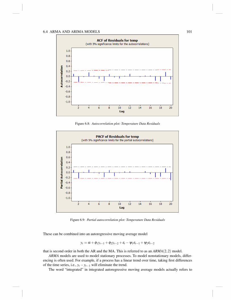
6.4 ARMA AND ARIMA MODELS 101

Figure 6.8: Autocorrelation plot: Temperature Data Residuals

Figure 6.9: Partial autocorrelation plot: Temperature Data Residuals

These can be combined into an autoregressive moving average model

yt = α +φ1yt−1 +φ2yt−2 + εt −ψ1εt−1 +ψ2εt−2

that is second order in both the AR and the MA. This is referred to as an ARMA(2,2) model.ARMA models are used to model stationary processes. To model nonstationary models, differ-

encing is often used. For example, if a process has a linear trend over time, taking first differencesof the time series, i.e., yt − yt−1 will eliminate the trend.

The word “integrated” in integrated autoregressive moving average models actually refers to

102 6. TIME SERIES

Figure 6.10: Individuals Control Chart: Temperature Data Residuals

differencing. An ARIMA(2,1,2) model is actually an ARMA(2,2) model for the series differencedseries yt − yt−1. In general, one can fit ARIMA(p,d,q) models which take d differences (a sec-ond order difference is analyzing wt −wt−1 where wt ≡ yt − yt−1) and fit p autoregressive terms(yt−1, . . . ,yt−p) and q moving average terms (εt−1, . . . ,εt−q).

It turns out that an ARIMA(0,0,1) leads to predictions that are essentially EWMAs. In the videocited earlier, Box mentions that he has found IMA(1,1) (ARIMA(0,1,1)) models to be very usefulin industrial applications.

6.5 Computing

Minitab is easy.

R code from my book ALM-III

rm(list = ls())

coal.production <- read.table(

"C:\\E-drive\\Books\\LINMOD23\\DATA\\ALM6-1.dat",

sep="",col.names=c("Year","Wt"))

attach(coal.production)

coal.production

#install.packages("forecast")

library(forecast)

MO=c(2,1,1)

fit = Arima(Wt,order=MO,include.constant=TRUE,method = "ML")

fit

Est=coef(fit)

SE=sqrt(diag(fit$var.coef))

6.6 EXERCISES 103

Tratio=Est/SE

Tabcd = c(Est,SE,Tratio)

TabCoef=matrix(Tabcd,I(MO[1]+MO[3]+1),3,dimnames = list(NULL,c("Est", "SE", "t")))

TabCoef

# Variance estimate

SSE = t(fit$residuals)%*%fit$residuals

# SSE/(length(Wt)-I(MO[1]+MO[2]+MO[3]+1))

# Eliminate "+1" if "constant=FALSE"

# Correlation Matrix

diag(1/SE,nrow=I(MO[1]+MO[3]+1))%*%fit$var.coef%*%diag(1/SE,nrow=I(MO[1]+MO[3]+1))

# Figs 7-5

par(mfrow=c(2,1))

Acf(residuals(fit),ylim=c(-1,1))

Pacf(residuals(fit),ylim=c(-1,1))

par(mfrow=c(1,1))

# Results not shown

# normal plot, periodogram

# fhat_5 spectral density

qqnorm(residuals(fit),ylab="Wt residuals")

spec.pgram(residuals(fit),taper=0,detrend=FALSE,fast=FALSE)

spec.pgram(residuals(fit),taper=0,detrend=FALSE,fast=FALSE,

kernel("daniell", 2))

# Fig 7-6

plot(Year,residuals(fit),type="b")

# Fig 7-7

fitpred=forecast(fit,7)

fitpred

Yearfuture=c(81,82,83,84,85,86,87)

Wtfuture=c(818.4,833.5,777.9,891.8,879.0,886.1,912.7)

plot(Year,Wt,type="l",xlim=c(20,87),ylim=c(300,925))

lines(Yearfuture,Wtfuture,type="l")

lines(Yearfuture,fitpred$mean,type="l",lty=5)

lines(Year,fit$fit,type="l",lty=5)

legend("topleft",c("Actual","ARIMA"),lty=c(1,5))

6.6 Exercises

EXERCISE 6.6.1 Dodson (1995) looks at “daily viscosity readings from an oil house that supportsa sheet metal rolling mill.” The data are in Table 6.2.

regress on time and look at residuals for time series effect.

104 6. TIME SERIES

Table 6.2: Oil house viscosity readings

304 314 307 315 297 304 314 321 307 321288 302 308 341 300 287 280 281 285 281283 287 281 285 291 281 283 284 291 278280 263 254 261 270 254 260 259 260 263268 270 253 253 247 247 256 256 260 237

Read across then down

Table 6.3: Finished product carbon black DBP values

pm am pm am3 7 11 3 7 11 3 7 11 3 7 1195 100 104 105 111 99 100 108 101 105 113 114

109 110 100 104 97 127 112 106 103 100 98 102103 103 98 103 102 106 93 98 108 111 107 10478 102 112 95 96 90 91 97 90 90 90 10097 97 93 98 101 98 94 98 100 94 97 10397 98 99 101 99 102 105 106 107 105 103 116

autoregress using least squares and look at resids for white noiseautoregress using ts procedure and look at residstime series plot shows downward trend. compute first differences and replot. fit a model.

EXERCISE 6.6.2. Schneider and Pruett (1994, qe94-348.dat) look at carbon black DBP valuesover 12 days with 6 readings per day at 3, 7, and 11, both AM and PM (days start at 3PM). The dataare in Table 6.3. Do a time series analysis. Look for day effects and for time within day effects.

EXERCISE 6.6.3. Consider again the data of Exercise 4.9.17 and Table 4.16.The data are repeated in Table 6.4. Look for autocorrelations within Heads.

Table 6.4: Outside diameter of injection molded bottles. (qe94-347.dat)

HeadSample 1 2 3 4

1 2.01 2.08 2.08 2.042 1.97 2.03 2.09 2.103 2.03 2.09 2.08 2.074 1.96 2.06 2.07 2.115 1.94 2.02 2.06 2.116 2.01 2.03 2.07 2.117 2.00 2.04 2.09 2.068 2.01 2.08 2.09 2.099 2.01 2.00 2.02 2.07

10 2.01 1.96 2.08 2.1111 1.99 1.99 2.09 2.1112 1.98 2.02 2.03 2.0813 1.99 1.98 2.05 2.0414 2.01 2.05 2.07 2.0815 2.00 2.05 2.06 2.0616 2.00 2.00 2.08 2.1417 2.01 2.00 2.05 2.1518 2.03 2.09 2.11 2.1219 1.99 2.10 2.09 2.0920 2.01 2.01 2.01 2.11

6.6 EXERCISES 105

EXERCISE 6.6.4. Reanalyze all of the individuals chart data from the Chapter 4 exercises as timeseries.

Chapter 7

Reliability

7.1 Introduction

The topic of reliability covers a wide spectrum of material. Here we introduce the analysis of time-to-event data. Time-to-event data involves measuring how long it takes for something to happen: aball bearing failure, an automobile crash, death due to cancer, etc. Analysis includes modeling andestimation of lifetime distributions and probabilistic methods for predicting and estimating meanlifetimes, survival probabilities, and survival times for both individual components and systems. Inparticular, we introduce some peculiarities that arise with time-to-event data

The first peculiarity of time to event data is some some new notation and concepts. Typically,we are concerned with the cumulative distribution function F and the probability density function fof random variables. With time to event data one is often interested in corresponding concepts, thereliability function R (known in biological applications as the survival function S) and the hazardfunction h. If you are testing how long a refrigerator lasts under stress, you may have to quit thestudy before all the refrigerators die. This creates censored data. Censored data seems much moreprevalent when dealing with biological applications than industrial, but it raises its ugly head inboth. These new ideas are introduced in Section 2.

The second peculiarity is that time to event data are often skewed rather than symmetric. Asa result, statistical analysis is often based on distributions other than the normal. Several of thesedistributions are introduced in Section 3.

In general, reliability deals with the study of the proper functioning of equipment and systems.Our main area of focus is component and system reliability, i.e., in finding the reliability of a com-plex system from the knowledge of the reliabilities of its components. For a more extensive intro-duction to the subject, see Hoyland and Rausand (1994) or Crowder et al. (1991). For an alternativeapproach based on Bayesian statistics see Hamada et al. (2008).

In addition to the study of lifetime or failure-free operating time for a system or piece of equip-ment, reliability can include broader aspects of a systems performance over time. This allows vary-ing levels of performance, possibility of repeated failures/repairs etc. It uses stochastic processes.e.g. Markov processes, to model system performance, cf. Huzurbazar (2004).

7.2 Reliability/Survival, Hazards and Censoring

7.2.1 Reliability and Hazards

Failure models are probability distributions used for modeling the time to failure of a component (orsystem) in reliability. Let T be the random time to failure of a unit, that is, the time from when theunit is put into operation until it first fails. For example, suppose T represents the time to breakageof a timing belt on a car. We could measure time here as calendar time but in this case a morerelevant measure of “time” is the miles driven by the car. Here T represents the number of milesdriven by car before the belt breaks and t = 0 is the mileage on the car when the belt was put intooperation. For the remainder of this chapter, we assume that T is continuously distributed on [0,∞)

107

108 7. RELIABILITY

with probability density function f (t) and cumulative distribution function (cdf)

F(t) = Pr(T ≤ t) =∫ t

0f (x)dx for t > 0. (7.2.1)

F(t) denotes the probability that the unit fails in the time interval (0, t]. By the Fundamental Theo-rem of Calculus, the probability density function is

f (t) =ddt

F(t). (7.2.2)

The reliability function of a unit is defined as

R(t)≡ 1−F(t) = P(T > t). (7.2.3)

This is the probability that the unit does not fail in the time interval (0, t] or, equivalently, theprobability that the unit is still functioning (survives) beyond the time t. In biological applicationsR(t) is often called the survival function and denoted S(t).

The probability that a unit fails in a short time, say, (t, t +δ t] is

Pr(t < T ≤ t +δ t) .= f (t)δ t (7.2.4)

Often, we are interested in the hazard function or failure rate function, denoted h(t), which is definedfrom the probability that the unit fails in a short time interval (t, t + δ t] given that it has not failedby time t, i.e.,

Pr(t < T ≤ t +δ t|T > t) =F(t +δ t)−F(t)

1−F(t).=

f (t)δ t[R(t)]

. (7.2.5)

Mathematically, the hazard is the rate at which this probability changes at time t, that is, the limit asδ t gets small of the conditional probability of the interval, divided by the length δ t of the interval,

h(t)≡ limδ t→0

Pr(t < T ≤ t +δ t|T > t)δ t

= limδ t→0

F(t +δ t)−F(t)[1−F(t)]δ t

=f (t)R(t)

.

The density function f (t) and the hazard function h(t) are mathematically interchangeable inthat knowing one determines the other but they answer different questions. Suppose at time t = 0we have a new unit and want the probability that this unit will fail in the interval (t, t +δ t]. This isapproximately equal to the probability density f (t) times the length of the interval δ t as given by(7.2.4). Now suppose that the unit has survived up to time t and we want to know the probability thatthis unit will fail in the next interval (t, t + δ t]. This probability is now the conditional probabilityin (7.2.5) and is approximately equal to the hazard function h(t) times the length of the interval δ t.

If the hazard h(t) is an increasing function of t, the chance of a failure becomes greater astime goes on. Such hazards are useful when the unit suffers from fatigue or cumulative damage. Ifthe hazard function is a decreasing function of t, the chance of a failure decreases with time. Thiscorresponds to the “burn-in” period for some electronic components where substandard units burnout early. If one restricts attention to an item’s mature period, the chance of failure is often constantover time, i.e., the hazard is flat. Household appliances often display this when they are neither veryyoung or old.

A bathtub shaped hazard function is often appropriate for the entire life of an item. Newlymanufactured items (refrigerators, automobiles, even infants) are subject to high initial hazards thatdecrease as they mature. (If something is fundamentally wrong, it tends to show up early.) Theitems then settle into a long period of maturity where the hazard is essentially constant. Finally, asthe items age or wear out, their hazards tend to increase again.

Figure 7.1 gives a bathtub hazard function showing the “burn-in”, useful life, and wear-outperiod of a component. This hazard is a combination of the three shapes discussed previously. The

7.2 RELIABILITY/SURVIVAL, HAZARDS AND CENSORING 109

0 1 2 3 4 5

1.01.2

1.41.6

1.82.0

Bathtub Hazard Function

x

y

Figure 7.1: Bathtub shaped hazard function.

“burn-in” or “infant mortality” period shows a high hazard initially which represents undiscovereddefects in substandard units. The “useful life” period is also called the “chance failure” period. Thisis the stable part of the unit’s life. As the unit ages, it enters it’s wear-out period. In practice, thishazard shape is difficult to use. Many units are tested via a quality control process before beingreleased to users so that the “infant mortality” period is removed. For mechanical units, the usefullife period often shows a slightly increasing tendency.

Often when analyzing failures we are restricted to limited age ranges of an item where the hazardshapes are constant, increasing, or decreasing. The Exponential distribution of the next section isoften useful because it has a flat hazard. Many of the models in the next section display either flat orincreasing hazards. Many include the Exponential as a special case. To have a flat hazard you musthave an Exponential distribution.

The mean time to failure (MTTF) of a unit is defined as

MT T F = E(T ) =∫ ∞

0t f (t)dt

where E(T ) is the expected value of the random variable T . The MTTF can also be expressed as

MT T F =∫ ∞

0R(t)dt.

In more complicated systems we might incorporate the time to repair an item, say, U . The meantime between failures (MTBF) is the MTTF plus the mean time to repair (MTTR), i.e..

MT BF = MT BF +MT T R = E(T )+E(U).

7.2.2 Censoring

Consider the joint distribution of T , the time to event, and a random variable C the determines thetime after which you will no long be able to observe T . If you started an experiment in the morningand have to quit and go home at 5PM, that determines C. In studies on people, C is when a person

110 7. RELIABILITY

becomes no longer available to the study. Perhaps they died. Perhaps they moved to another town.Perhaps they tired of the hassle of being studied. Censoring is particularly convenient when it occursindependently of the time T being studied. But if you think about the event being death, the closerdeath, gets the more likely one is to quit a study. When subject to censoring, the actual data observedare

(X ,δ )≡{(T,1) if T ≤C(C,0) if C > T .

δ is a random indicator for not being censored. (That does not keep people from sometimes callingit the censoring indicator.) Let fT be the density for T and fC the density for C. The likelihood forobserving X = u and δ is defined as

fT (u)δ ST (u)1−δ .

7.3 Some Common Distributions

Commonly used distributions for modeling the skewed data associated with time to event data arethe Exponential, Lognormal, and Weibull. Another useful distribution is the Gamma.We now intro-duce these.

7.3.1 Exponential Distributions

The exponential distribution is the most widely used in reliability mainly because of its tractabilityand nice properties. We have already mentioned that it has a flat hazard function. It also has amemoryless property that

Pr(T > t +u|T > t) = Pr(T > u)

and the minimum of several iid Exponentials is again an Exponential (but with a different parame-ter).

The are two different parameterizations for the Exponential distribution that are in common use.The density, cdf, reliability, and hazard functions are given by

f (t) = θ exp(−θ t) for θ > 0, t > 0,F(t) = 1− exp(−θ t),

R(t) = exp(−θ t),

h(t) =θ exp(−θ t)exp(−θ t)

= θ , (7.3.1)

or by

f (t) = (1/λ )exp(−t/λ ) for λ > 0, t > 0,F(t) = 1− exp(−t/λ ),

R(t) = exp(−t/λ ),

h(t) =(1/λ )exp(−t/λ )

exp(−t/λ )= 1/λ . (7.3.2)

We will use the first parameterization and indicate T having an exponential distribution by T ∼Exp(θ). Note that if X ∼ Exp(1) then T ≡ X/θ ∼ Exp(θ).

7.3.2 Weibull Distributions

Weibull distributions are a straightforward generalization of the exponential. If X ∼ Exp(θ) thenT = X1/α has a Weibull(α,θ) distribution when the Weibull is parameterized as

f (t) = αθ tα−1 exp(−θ tα) for θ > 0, α > 0, t > 0

7.3 SOME COMMON DISTRIBUTIONS 111

F(t) = 1− exp(−θ tα)

R(t) = exp(−θ tα)

h(t) = αθ tα−1.

An alternate parameterization is

f (t) =α

λ

( tλ

)α−1exp[(−t/λ )α ] for λ > 0, α > 0, t > 0

F(t) = 1− exp[(−t/λ )α ]

R(t) = exp[(−t/λ )α ]

h(t) =(

α

λ α

)tα−1.

For α = 1 this is the exponential. For α > 1 the hazard function is increasing as a power of t. Forα < 1 the hazard is decreasing.

7.3.3 Gamma Distributions

Gamma distributions are a less straightforward generalization of the exponential.The are two different parameterizations for the Gamma distribution that are in common use.

f (t) =β α

Γ(α)tα−1e−β t for α > 0, β > 0, t > 0

or

f (t) =1

Γ(α)λ αtα−1e−t/λ for α > 0, λ > 0, t > 0.

There are no particularly nice functional forms for the cdf, reliability function, or hazard. α is knownas the shape parameter, β is a scale parameter.

Using the Gamma(α,β ) parameterization, a Gamma(1,θ) is an Exp(θ).

7.3.4 Lognormal Distributions

If X ∼ N(µ,σ2) then Y = log(X) has a lognormal distribution with median eµ and scale parameterσ . Turns out the the mean is exp[µ +(σ2/2)].

7.3.5 Pareto

This is primarily of interest because it has a decreasing hazard function. It can be constructed asa mixture of exponential distributions using gamma distribution weights. (To a Bayesian, it is themarginal distribution of the data for a conditional distribution that is exponential and a prior that isgamma.)

f (t) =βαβ

(t +α)β+1 for α > 0, λ > 0, t > 0,

F(t) = 1−(

α

t +α

)β

,

R(t) =

(α

t +α

)β

,

h(t) = β/(t +α).

112 7. RELIABILITY

Table 7.1: Plackett-Burman L12 Screening design for thermostats

Trial A B C D E F G H I J K1 0 0 0 0 0 0 0 0 0 0 02 0 0 0 0 0 1 1 1 1 1 13 0 0 1 1 1 0 0 0 1 1 14 0 1 0 1 1 0 1 1 0 0 15 0 1 1 0 1 1 0 1 0 1 06 0 1 1 1 0 1 1 0 1 0 07 1 0 1 1 0 0 1 1 0 1 08 1 0 1 0 1 1 1 0 0 0 19 1 0 0 1 1 1 0 1 1 0 010 1 1 1 0 0 0 0 1 1 0 111 1 1 0 1 0 1 0 0 0 1 112 1 1 0 0 1 0 1 0 1 1 0

Table 7.2: Number of temp cycle changes before thermostat failure.

Trial Data1, , 957, 2846, 7342, 7342, 7342, 7342, 7342, 7342, 7342, 7342,2, , 206, 294, 296, 305, 313, 343, 364, 420, 422, 543,3, , 63, 113, 129, 138, 149, 153, 217, 272, 311, 402,4, , 76, 104, 113, 234, 270, 364, 398, 481, 517, 611,5, , 92, 126, 245, 250, 390, 390, 479, 487, 533, 573,6, , 490, 971, 1615, 6768, 7342, 7342, 7342, 7342, 7342, 7342,7, , 232, 326, 326, 351, 372, 446, 459, 590, 597, 732,8, , 56, 71, 92, 104, 126, 156, 161, 167, 216, 263,9, , 142, 142, 238, 247, 310, 318, 420, 482, 663, 672,

10, , 259, 266, 306, 337, 347, 368, 372, 426, 451, 510,11, , 381, 420, 7342, 7342, 7342, 7342, 7342, 7342, 7342, 7342,12, , 56, 62, 92, 104, 113, 121, 164, 232, 258, 731

7.4 An Example

Bullington, Lovin, Miller, and Woodall (1993) examine the number of temperature cycle changes athermostat endures before failure. They examined 11 factors each at 2 levels that were thought topossibly affect the performance.A: Diaphram Plating Rinse (clean primary – pure secondary, contaminated primary – no secondary)B: Current Density (5 min at 60 amps, 10 min at 15 amps)C: Sulfuric Acid Cleaning (3 sec, 30 sec)D: Diaphragm Electroclean (2 min, 12 min)E: Beryllium Copper Grain Size (0.008in, 0.018in)F: Stress Orientation (perpendicular, in line – relative to seam weld)G: Humidity (wet, dry)H: Heat Treatment (45 min, 4hrs – at 600◦ F)I: Brazing Machine (no cooling water or flux – excess water, 3 times normal flux)J: Power Element Electroclean (like D)K: Power Element Plating Rinse (like A)

This determines 211 treatment combinations of which only 12 were observed as indicated in Ta-ble 7.1 wherein 0s indicate the first factor level as given above.

Table 7.1 is a Placket-Burman design as discussed in TiD and a Taguchi L12 design as discussedin Chapter 11 and TiD. Table 7.2 contains the 10 observations on each observed treatment combi-nations.

Rather than doing a full analysis of this complicated design, use one treatment to illustrate a one

7.4 AN EXAMPLE 113

sample problem and two treatments to illustrate two sample problems. Introduce censoring fromsome trials.

Some Random Thoughts

give an example early on to motivate these things. why does anyone really care about R(t) or h(t)?The first couple of things are bullets to be worked into an example

• Nuclear reactor safety study. Need to look up.• Germany WWII; V1 missile. First 10 were fiascos. Careful attention was paid to details but first

10 exploded on the launch pad or landed “too soon” in the English channel. Later, people thoughtabout probability for series components.P(system works)= ∏ P(individual components work)¡¡ P(any one component works)

Imagine we have 10 components in series. Each has prob 0.90 of working. Prob the system worksis .910 = .3486 which is far less than the prob of any individual component working.• Point out that this will only get worse when we have components in series and parallel as is the

case with a full-fledged missile or even your washing machine...start with what is reliability in general

Things to add possibly• repairable systems. k out of p systems, system functions when ≥ k components work properly.

Chapter 8

Random Sampling

Random sampling is the tool used to ensure that samples are collected without bias. It is all too easyfor people to choose samples that will bias the results of the study. If one is studying how much milkschool children drink in a school district, a sample chosen by the whim of teachers would probablybe biased. The students chosen would probably not be representative of the students as a whole. Infact, they may well be chosen (perhaps subconsciously) to reinforce the attitudes of the teacher.

If a shipment of automobile components were being evaluated to check the rate of defectives,the containers at the front of the shipment may not be representative of the entire shipment. Thiscould happen if the supplier is disreputable and suspects that you will only sample those crates thatare easy to sample. More realistically (we hope) the state of the production process can change overtime and so when crates are placed for shipment, they are placed in time order, so where you sampleis related to the time of production. Random sampling is a device for selecting a sample that has nosystematic bias.

8.1 Acceptance Sampling

Suppose you manufacture audio equipment and you have just received a shipment of electricalcomponents. How do you decide whether these components are of sufficiently high quality for yourmanufacturing process?

By far the best way to do this is to have a history with the supplier which tells you that they are areputable firm. Then, have the supplier show you the control charts they used in production. Basedon the control charts, if the manufacturing process was under control and meeting specifications,you can purchase the item without reservations.

What if you don’t trust the supplier to show you accurate control charts? Why are you dealingwith a supplier like that? What if this is a new supplier that does not have control charts? Why areyou dealing with a supplier like that? We could go on and on like this, but the fact is that sometimespeople end up making purchases under less than optimal conditions. In such situations, how canyou decide whether to accept a shipment of components or not. A reasonable method is to take arandom sample of the shipment and inspect the sample to learn about the shipment as a whole.

Deming would probably argue that while sampling may be reasonable to determine what todo with the entire shipment, once the decision is made to use the components, sampling shouldeither cease or every single component should be inspected to determine if it meets specifications.Juran and Gryna (1993) give reasons for performing acceptance sampling but they suggest thatacceptance sampling should be used in an overall quality control process designed to eliminate theneed for acceptance sampling. Some situations where sampling is important are destructive testing(in which to test a product you have to destroy it), expensive testing (in which the cost of examiningevery unit is excessive), situations where production is continuous, so that no natural definitionof a manufacturing unit exits (examples of this are textiles, thread, paper, photographic film, etc.)and where production runs are too large and too fast, so that there are too many units to inspect(examples include the production of nuts, bolts, screws, etc.).

115

116 8. RANDOM SAMPLING

8.2 Simple Random Sampling

Suppose a shipment of automobile components contains N = 300 units. Suppose we want to takea sample of n = 50 of these units to inspect for defectives. To take a simple random sample, wehave to make a list of all 300 units, assigning each a number between 1 and 300. It doesn’t matterhow we make the list as long as each unit appears once and only once on the list. It could be a listof serial numbers or, if the components were delivered on a palate in crates, one to a crate, we canjust imagine assigning a number to each crate on the palate. Using a method for generating randomnumbers, you randomly select 50 numbers between 1 and 300 without replacement. Having obtainedthe 50 numbers, go back to the list and identify the automobile components that correspond to thenumbers on the list. These are the automobile components that need to be inspected for defects.

The Minitab commands below will make such a selection and list the 50 numbers in column C2.

set c1

1:300

end.

sample 50 c1 c2

Or you can enter the same information by navigating the menus:Calc > Make Patterned Data > Simple Set of Numbers

Calc > Random Data > Sample from Columns

To fix ideas we present an artificially small example.

EXAMPLE 8.2.1 A collection of N = 40 video tapes, I mean DVDs, I mean downloads, no I reallydo mean DVDs, of the popular English costume comedy Blue Asp were obtained. The running timesof these DVDs are designed to be exactly 34 minutes. Each DVD is clearly identified and assigneda number from 1 to 40. A simple random sample of size n = 5 from the numbers between 1 and 40gave 9, 23, 13, 38, 6. The 5 DVDs corresponding to these numbers were pulled out of the collectionand the running times of the DVDs were measured. The run times were 34.610, 34.743, 34.480,34.239, 33.939. The estimate of the population mean running time is the sample mean running time

µ ≡ x =x1 + x2 + · · ·+ xn

n=

34.610+34.743+34.480+34.239+33.9395

= 34.4022

The estimate of the population variance is the sample variance

s2 =1

n−1

n

∑i=1

(xi− x)2

=1

5−1[(34.610−34.4022)2 + · · ·+(33.939−34.402)2]

= 0.1016417

The usual standard error of x from an introductory statistics course is

SE(x) =

√s2

n

with a 95% confidence interval for the population mean running time of

x±2SE(x).

Alas, a slight modification of the standard error is necessary in our current situation. The usualresults given above assume that either the population being sampled is infinitely large or that thesampling occurs with replacement. Sampling with replacement means that after an object has beensampled from the population, it is placed back into the population so that it has the possibility of

8.3 STRATIFIED RANDOM SAMPLING 117

being sampled again. That is not how simple random sampling is conducted in practice. In practice,sampling is without replacement. Once an object has appeared in a sample, it cannot appear again.This actually causes the sampling to be more accurate. If you take a simple random sample withreplacement of size 5 from a population of size 5, you may or may not see every element in thepopulation. If you take a simple random sample without replacement of size 5 from a populationof size 5, you are guaranteed to have seen every element in the population and the sample mean isguaranteed to equal the population mean. Similarly, there will be less variability in x for a sampleof size 5 from a population of size 40 when sampled without replacement, than there will be if thepopulation is sampled with replacement. The difference can be accounted for by a finite populationadjustment,

1− nN

where n is the sample size and N is the population size. The sample mean and variance withoutreplacement remain

µ ≡ x =x1 + x2 + · · ·+ xn

n= 34.4022

and

s2 =1

n−1

n

∑i=1

(xi− x)2

= 0.1016417

but now, using the finite population adjustment,

SE(x) =

√(1− n

N

) s2

n=

√(1− 5

40

)0.1016417

5= 0.13337.

With this new standard error, the 95% confidence interval is

x±2SE(x)

or34.4022±2(0.13337)

for in interval of (34.135,34.669). The interval does not contain the target value 34, so the DVDsseem to be running longer than they are supposed to run.

It turns out that for sampling without replacement

E(x) = µ, Var(x) =σ2

n

(1− n−1

N−1

), E(s2) = σ

2 NN−1

.

From these it is not difficult to show that

E[(

1− nN

) s2

n

]= Var(x).

Note that, whenever n approaches N, Var(x) approaches 0 and that, as N gets large, these approachthe usual sampling with replacement results.

8.3 Stratified Random Sampling

Suppose you have bought automobile components from a company, but the parts delivered comefrom three different manufacturing plants. For production purposes, it is probably best to just treat

118 8. RANDOM SAMPLING

these as three different shipments and evaluate the quality of the three shipments separately. How-ever for some purposes, perhaps cost accounting, it may be necessary to get an estimate of theoverall total number of defectives coming from this company. The appropriate technique is to takea simple random sample of components from each of the plants and to combine the results appro-priately. In this context, each of the plants is referred to as a strata and taking random samples fromeach strata is referred to as stratified random sampling.

EXAMPLE 8.3.1 In addition to the Blue Asp DVDs obtained in Example 8.2.1, two other ship-ments of DVDs were obtained at a later time, each of which included 30 DVDs. We want to estimatethe population mean of all 100 DVDs. We begin by taking simple random samples without replace-ment from each of the three shipments (strata). For illustrative purposes, the sample from the firstshipment is as in Example 8.3.1 and the samples from the other two shipments are of sizes 4 and 6,respectively. The samples are

Stratum Ni Sample1 40 34.610, 34.743, 34.480, 34.239, 33.9392 30 34.506, 34.734, 34.350, 34.5093 30 34.016, 34.347, 34.084, 34.932, 34.605, 34.437

Summary statistics are given below. Subscripts are used to indicate the stratum associated witha stratum size, a sample size, a sample mean, or a sample variance. For example, N1 = 40, n1 = 5,x1 = 34.4022, and s2

1 = .1016417 are all from stratum 1.

Stratum Ni ni xi s2i

1 40 5 34.4022 0.10164172 30 4 34.52475 0.024974253 30 6 34.4035 0.1152931

The estimate of the mean of the entire population is a weighted average of the stratum samplemeans. The weights are relative to the size of the strata Ni. Let

N = N1 +N2 +N3 = 40+30+30 = 100

µ =3

∑i=1

Ni

Nxi

=40

10034.4022+

30100

34.52475+30100

34.4035

= 34.439355

The variance of the estimate is

Var(µ) =3

∑i=1

(Ni

N

)2

Var(xi)

so, using the results on simple random sampling for each strata (which includes incorporating thefinite population corrections for sampling within each strata), the standard error is,

SE(µ)

=

√√√√ 3

∑i=1

(Ni

N

)2(1− ni

Ni

)s2

ini

=

[(40

100

)2(1− 5

40

)0.1016417

5+

(30

100

)2(1− 4

30

)0.02497425

4

+

(30

100

)2(1− 6

30

)0.1152931

6

]1/2

= 0.068676653

8.4 CLUSTER SAMPLING 119

A 95% confidence interval for the mean has endpoints µ±2SE(µ), which is

34.439355±2(0.068676653)

giving the interval (34.302, 34.577).

8.3.1 Allocation

One question about stratified samples is how do you decide how many samples to take in eachstratum. One relative safe way, is to use proportional allocation of the samples. In proportionalallocation, for an over all sample size of n, you choose ni observations from stratum i where ni ischosen to satisfy

ni

n=

Ni

NNote that the total number of units in the ith stratum, Ni, and the total number of units in thepopulation, N, are both assumed to be known.

If you have some idea about how much it costs to collect an observation in each stratum andif you also have some idea of the variance in each stratum, one can find an optimal allocation. Inoptimal allocation, you will want to take more observations in strata with more variability and fewerobservations in strata for which the cost per observation is more. These issues are discussed in moredetail in any good book on sampling, e.g., Lohr (1999).

8.4 Cluster Sampling

Suppose again that the automobile components have been crated and put on a palette, but that nowthese are small components and that there are 20 components in each crate. To simplify life, letsassume that they all come from the same plant. The obvious way to sample is to make a list of cratesand take a simple random sample of crates. Once the crates have been selected, either we can inspectall 20 of the components in each crate, or for each crate we can take a further random sample of the20 components and inspect only those components chosen in the second stage of sampling. The firstof these procedures is referred to as one-stage cluster sampling, the second procedure is referred toas two-stage cluster sampling.

EXAMPLE 8.4.1 One-stage cluster sampling.Suppose Blue Asp DVDs are boxed in cartons of 20 to 25 and a wholesaler gets a shipment of 100cartons. Suppose the wholesaler wants to estimate the population mean running length of a DVDbased on taking a sample of 3 cartons. This is a very small sample but it will illustrate the ideas. Thisinvolves sampling 3 cartons and measuring the running time for each DVD in the carton. Implicitlywe are assuming that DVDs in a carton are probably more alike that DVDs in different cartons.

Carton Ni xi1 20 34.4132 23 34.5353 25 34.414

Note that both the carton sizes and the carton means are random variables but only because we havea random selection of cartons. 2

In general let c denote the number of clusters (cartons) in the population. Let the pair (Nk,Tk)denote the number of items in the kth cluster and the total of all the measurements made on theitems in the kth cluster. (The total might be the total number of defectives in the cluster.) NoteTk = Nkxk where xk is computed from the xk js involving the jth observation from the kth cluster.

120 8. RANDOM SAMPLING

The population mean of the xk j population is the sum of all the cluster totals Tk divided by the sumof all the cluster sizes Nk, i.e.,

µ =∑

ck=1 Tk

∑ck=1 Nk

=∑

ck=1 Nkxk

∑ck=1 Nk

=∑

ck=1 ∑

Nkj=1 xk j

∑ck=1 Nk

. (8.4.1)

The odd thing about cluster sampling is that we are not directly sampling from our populationof interest, the xk js. And, unlike our previous problems, we do not even know the size of the xk jpopulation. We know the number of clusters c but we do not know the size of every cluster. Thismeans that, unlike our previous scenarios, we need to estimate both the numerator and denominatorof equation (8.4.1).

Take a random sample of n clusters giving us random pairs (Ni,Ti), i= 1, . . . ,n. The mean clustersize is

N =∑

ni=1 Ni

n,

so the estimated xk j population size is cN. The estimated mean cluster total is T so the estimated xk jtotal is cT . The estimated xk j population mean is

µ =cTcN

=TN

=∑

ni=1 Ti/n

∑ni=1 Ni/n

=∑

ni=1 Ti

∑ni=1 Ni

=∑

ni=1 Nixi

∑ni=1 Ni

. (8.4.2)

The usual standard error is approximated by treating the Nis as fixed so that all the randomnessis associated with T ,

SE(µ) = SE(

TN

).=

1N

SE(T ) =1N

√(1− n

c

) s2Tn

where, again treating Ni as fixed so that E(Ti) = Niµ ,

s2T =

1n−1

n

∑i=1

(Ti−Niµ)2 =

1n−1

n

∑i=1

(Nixi−Niµ)2 =

1n−1

n

∑i=1

N2i (xi− µ)2.

EXAMPLE 8.4.1 CONTINUED. One-stage cluster sampling.Applying the formulae to our DVD example gives.

µ =20(34.413)+23(34.535)+25(34.414)

20+23+25= 34.45463.

s2T =

[202(34.413− µ)2]+ [232(34.535− µ)2]+ [252(34.414− µ)2)]

2= 2.570979,

SE(µ) =1

22.6666666

√(1− 3

100

)s2

T3

= 0.04022415.

A 95% confidence interval is34.45463±2(0.04022415).

or (34.37418, 34.53508).The variance and standard error are ugly arithmetic so I wrote R code:

muhat=((20 *34.413) + (23 * 34.535) + (25 *34.414))/68

muhat

sT2=( (20^2 * (34.413-muhat)^2) + (23^2 * (34.535-muhat)^2) +

(25^2 *(34.414-muhat)^2))/2

8.4 CLUSTER SAMPLING 121

sT2

se=sqrt( (1-(3/100))*sT2/3 )/22.6666666

se

muhat+(2*se)

muhat-(2*se)

2

EXAMPLE 8.4.2 Two-stage cluster sampling.Measuring the running length of each DVD in a carton of 20 seems excessive. It might be morereasonable to randomly select a smaller number of DVDs out of each carton and measure the runninglength on just those DVDs.

In our example we have c = 100 clusters from which a sample of n = 3 is taken. The size of eachcluster in the sample is Ni and the size of the sample within each cluster is ni. Summary statisticsfor our example of DVD lengths are:

Carton Ni ni xi s2i

1 40 5 34.4022 0.10164172 30 4 34.52475 0.024974253 30 6 34.4035 0.1152931

In one-stage cluster sampling we looked at every DVD in the carton, so we did not need to considers2

i , the variance associated with sampling from (within) the carton 2

In a technical sense, two-stage cluster sampling is very similar to stratified sampling in whicheach cluster is thought of as a stratum. The key difference is that in stratified sampling, we collecta sample from every stratum (cluster) and in two stage cluster sampling we only take a sample ofthe clusters (strata). As a result, the formulae for two-stage cluster sampling include both stratifiedsampling and one-stage cluster sampling as special cases. Stratified sampling is where we take acomplete sample of all the clusters (strata) and one-stage cluster sampling is where the samplewithin the clusters contains all of the units within the cluster. Ideally, we would perform stratifiedsampling when there is a lot of variability between clusters and not much variability within them,and we would perform one-stage cluster sampling when there is little variability between clustersand a lot of variability within them, but, in practice, what we perform is usually determined byphysical characteristics of the population.

Our population of interest is the xkhs, k = 1, . . . ,c, h = 1, . . . ,Nk. Again, Tk = ∑Nkh=1 xkh is the total

from the kth cluster and just as in equation (8.4.1),

µ =∑

ck=1 Tk

∑ck=1 Nk

.

Again, we need to estimate both the numerator and the denominator.In two-stage cluster sampling we take a first-stage sample of n clusters from the population of

c clusters The second-stage sample from the ith cluster involves determining Ni as well as taking asample of size ni, say xi j, j = 1, , . . . ,ni. To estimate the total in the ith cluster, we use Ti = Nixi. Theestimated xk j population mean is a minor modification of (8.4.2),

µ =∑

ni=1 Ti

∑ni=1 Ni

=∑

ni=1 Nixi

∑ni=1 Ni

.

The estimated population mean can also be written as,

µ =1N

∑ni=1 Nixi

n. (8.4.3)

The standard error now has to incorporate not only the variability due to looking at only n of

122 8. RANDOM SAMPLING

c clusters but also the variability of estimating the total Ti from the sampled clusters. The formerinvolves a version of s2

T and the latter involves the within cluster sample variances s2i .

SE(µ) =1N

√(1− n

c

) s2Tn+

1nc

n

∑i=1

(1− ni

Ni

)N2

is2

ini. (8.4.4)

The formula

s2T =

1n−1

n

∑i=1

(Nixi−Niµ)2

looks the same as for one-stage cluster sampling but the components xi and µ are computed differ-ently in two-stage cluster sampling.

Sometimes the size is known for every cluster in the population. In that case, N should bereplaced in (8.4.3) and (8.4.4) by N ≡ (N1 + · · ·+Nc)/c, the population mean of the cluster sizes.

Note that if n = c, we get the formulae for stratified sampling and, if ni = Ni for all i, we get theformulae for one-stage cluster sampling. So these two-stage formula are really the only ones youneed to know from this chapter!

EXAMPLE 8.4.2 CONTINUED. Two-stage cluster sampling.Applying the formulae to the two-stage DVD data,

µ =40(34.4022)+30(34.52475)+30(34.4035)

40+30+30= 34.43935,

s2T =

[402(34.4022− µ)2]+ [302(34.52475− µ)2]+ [302(34.4035− µ)2]

2= 5.414398,

n

∑i=1

(1− ni

Ni

)N2

is2

ini

=

(1− 5

40

)402 0.1016417

5+

(1− 4

30

)302 0.02497425

4+

(1− 6

30

)302 0.1152931

6= 47.16483.

SE(µ) =(

133.3333333

)√(1− 3

100

)s2

T3+

13(100)

[47.16483] = 0.04143772.

The 95% confidence interval is

34.43935±2(0.04143772)

or (34.35648, 34.52223). The estimate of the population size N is cN = 100(33.3333333) = 3333.Again I wrote R code:

muhat=((40 *34.4022) + (30 * 34.52475) + (30 *34.4035))/100

muhat

sT2=( (40^2 * (34.4022-muhat)^2) + (30^2 * (34.52475-muhat)^2) +

(40^2 *(34.4035-muhat)^2))/2

sT2

sisum=( 1 - (5/40) )*40^2 *(0.1016417/5) +

( 1 - (4/30) )*30^2 *(0.02497425/4) + ( 1 - (6/30) )*30^2 *(0.1152931/6)

sisum

se=(1/33.3333333) * sqrt( (1-(3/100))*sT2/3 + (1/(3*100)) * sisum)

se

muhat+(2*se)

muhat-(2*se) 2

8.5 FINAL COMMENT. 123

8.5 Final Comment.

There are many reasons for collecting accurate information about a body of material (population).The methods presented here are useful for these purposes. However, the worst reason for conductinga sample survey of a population is to determine the percentage of defective units in that population.The only acceptable proportion of defective units should be 0. Attention should be focused on prod-uct improvement, not the bean counting of how often things have gone wrong. Fixing the blame fordefects does not fix the problem that created the defects. The blame properly belongs to a manage-ment system that allows things to go wrong. Quantifying the extent of the problem can only helpwhen determining which problems are most important to fix first. Quantifying the problem alsogives no help in identifying how to fix the problem. Other statistical procedures can help with that.

Chapter 9

Experimental Design

To find out the effect of changing a process, it is generally necessary to change the process. Tofind out if a chemical reaction works better at 200 degrees than it does at 190 degrees, you needto set the process up to work at 200 degrees and see what happens. Seeing what happens when theprocess strays up to 200 degrees may be a good reason to investigate behavior at 200 degrees, butthere is no assurance that the process will work the same when set to 200 degrees as it did whenit strayed to 200 degrees. There was some reason for the process straying to 200 degrees, and anynumber of factors other than the temperature could be responsible for the observed improvement.To be sure that the cause of the improvement is the change in temperature, an experiment mustbe run. In an experiment, material is usually selected with as little variability as possible (whilestill characteristic of typical operating conditions) and the treatments (temperatures) are randomlyassigned to the material.

The quality of fiberglass shingles is tested using an Elmendorf tear test. TAMKO Roofing Prod-ucts of Joplin, MO was interested in evaluating the testing procedure. For their purposes, theyneeded a material to test with very little intrinsic variability so that the observed variability wouldbe due to the variability of the measurements rather than the variability of the material. It was even-tually decided to test the tear strength of vinyl floor covering under specified conditions. Two 1 footby 6 foot pieces were purchased and cut into five 1 foot squares. The squares were cut into 3-inby 2.5-in specimens. Four trained Elmendorf operators were each given a stack of 10 randomizedspecimens and instructed to test them in order. The experiment is well suited for identifying anydifferences in performance due to the four operators and estimating the variability associated withthe measurements. In reality, this is a brief synopsis of a data collection regime presented in Phillipset al. (1998) for evaluating the variability of the tear testers.

Experimental data are the only data that can be reliably used to determine cause and effect.Observational data can be used to establish that groups are different but observational data cannot beused to establish why groups are different. For example, if one has data on the ages at which nativeamericans, hispanics, and non-hispanic caucasians commit suicide, one may be able to establishthat these groups differ in the average ages at which they commit suicide, cf. Koopmans (1987)and Christensen (1996, Chapter 5). However, knowing that there are differences in the groups doesnothing to explain why there are differences in the groups. It does nothing to establish cause andeffect. Statistical data analysis is incapable of establishing cause and effect. Other ideas beyond dataanalysis are necessary for establishing this.

Statistical experiments are characterized by using random numbers to assign experimental treat-ments to experimental material. It is this use of random numbers that logically allows one to infercause and effect from statistical experiments. Using random numbers to assign treatments to ma-terial eliminates any systematic biases among the groups of material associated with a treatment.Since there can be no systematic differences between the groups of material to which the treatmentswere applied, any differences observed between the treatment groups must be caused by the treat-ments. Note that the data analysis only establishes that the groups are different, it is the experimentalprocedure that allows one to infer that the differences are caused by the treatments.

For example, suppose one were to study the effect of giving young school children a cup of

125

126 9. EXPERIMENTAL DESIGN

milk each day. In each of several classrooms, half the children are given a cup of milk and half thechildren are not. At the end of the school year, measures of student performance are taken. Leftto their own devices, the classroom teachers may well give the milk to the half of their class thatseem to “need” the milk most. In other words, they may give the milk to those students with thelowest socio-economic status. Most measures of student performance are highly correlated withsocio-economic status, and a cup of milk each day is unlikely to overcome those differences. Thus,by giving the milk to the most needy students, the teachers are assuring that, as a group, studentswho are given a cup of milk each day will perform worse than students who do not receive milk. Toaccurately measure the effect of giving out a cup of milk each day, those receiving the milk must bechosen randomly, so that there are no systematic differences between the experimental groups otherthan the experimental treatments. Similar phenomena can easily occur in industrial experiments. Inthe tear testing example, the experimental material (pieces of vinyl floor covering) were preparedfirst and then randomly assigned to the operators. When assigning treatments in an experiment,most definitely, the squeaky wheel does not necessarily get the grease. A true experiment requiresrandomly assigning treatments to experimental units. Anything else is an observational study.

Great care must be used in setting up an experiment so that the treatments are actually whatthey were designed to be. Once the experimental material has been randomly assigned to treatmentgroups, a treatment becomes everything that systematically happens to that experimental group.Suppose you randomly assign rats to two groups and give one a drug and the other a placebo. Ifthe rats in the “drug” group develop cancer at a much higher rate than the placebo group, does thatimply that the drug caused the additional cancers? Not if you were storing the drug rats in an areacontaminated by asbestos (and the placebo rats someplace else)! The “treatments” can logically besaid to be causing the extra cancer, but the “drug” treatment is actually the combination of the drugand the asbestos and anything else that was systematically different for the “drug” group than forthe “placebo” group. It is important not to confuse the treatment with the label for the treatment.Even more importantly, one needs to set up experiments so that the treatment is as close as possibleto being what was originally meant by the treatment label.

Some conditions that one would like to study cannot be random assigned to experimental ma-terial, e.g., sex cannot be randomly assigned to people. So it is impossible to conduct a statisticalexperiment with sex as a treatment. Moreover, sexes are labels for such broad collections of traitsthat differ between two populations that it would be difficult to ever think of describing sex as theimmediate cause of anything that would require an experiment to establish. Sex groups may be dif-ferent, but what is it about being female that makes them behave or respond differently than males?

One final word needs to be said about randomization as the basis for concluding that treatmentscause observed effects. Randomization really only applies over the long run. It is possible, thoughunlikely, that systematic differences will occur in the treatment groups as the result of randomiza-tion. It is possible, unlikely but possible, that all of the “good” experimental material will randomlyget assigned to one treatment group. If you see that that has happened, then you should do some-thing about it. Unfortunately, if you don’t know what constitutes “good” material, you cannot becognizant of this happening. In the long run, over many replications of the experiment, such thingscan only occur with a very low frequency. So in the long run, randomization gives a firm basis forcause and effect conclusions. But one still needs to be careful in each particular case.

In medicine, specifically in epidemiology, people take another approach to establishing causeand effect. In statistical experiments, the idea is to create a pool of experimental material and thenrandomly assign treatments to the experimental material. The only systematic differences in theexperimental material are the treatment differences, hence treatments cause observed effects. Theepidemiologic approach is to try to adjust for every systematic difference in the treatment groups.If one properly adjusts for every systematic difference in the treatment groups, and differencesbetween the treatment groups remain after all of this adjustment, the differences must be due to thetreatments. This is a reasonable idea. The difficulty is in the execution. How does one appropriatelyadjust for every (important?) systematic difference in the treatment groups? In a medical examplea variety of factors immediately present themselves as candidates for adjustment: height, weight,

9.1 ONE-WAY ANOVA 127

Table 9.1: Summary Statistics, Vinyl Covers

VinylCover N yi· s2

iA 10 2273.6 16466.5B 10 2412.8 39867.7C 10 2222.4 11517.2

blood pressure, cholesterol, etc. But how does one ever know that all the important factors havebeen taken into account? That presumes one knows all of the important factors. Moreover, howdoes one ever know whether the form of these adjustments has been appropriate?

When studying ages of suicides for three racial groups, one might decide to adjust for varioussocio-economic factors. Were there differences in the three racial groups? Yes. Were there differ-ences in the three racial groups after adjusting for socio-economic factors? Whether “yes” or “no”,it is merely the answer to a slightly different question. And in this case, if differences exist, thatwill still never tell us what it is about the lives (social or genetic) of these groups that cause suchdifferences.

Two primary goals of experimental design are to reduce the variability that treatment com-parisons are subject to and to provide for a valid estimate of the variability of observations andestimates. There are several standard experimental design techniques for providing valid varianceestimates and reducing variability. The completely randomized design gives a valid variance esti-mate. Variance reduction is generally attained by comparing treatments within blocks of relativelyhomogeneous experimental material. Randomized complete block designs, Latin Square designs,and incomplete block designs all use forms of blocking to reduce variability and all provide forvalid estimates of variances.

Two additional features of experimental design will be discussed. In Section 4 we discuss a veryefficient way of defining treatments for an experiment. This is called creating a factorial treatmentstructure. In Chapter 10 we discuss fractional replications, which provide methods for obtaininginformation on the main effects of many factors using relatively few observations.

9.1 One-way Anova

One-Way ANOVA is a method for evaluating whether different groups have the same mean value.It may seem curious that a method for evaluating means would be called “analysis of variance” butwe will show why that is.

EXAMPLE 9.1.1 Vinyl Floor Covering Data.Table 2.3 gives data on tear test values for three vinyl floor coverings. In Section 2.4 we usedbox plots to compare the three coverings. Here we present a more formal approach to evaluatingwhether the groups have different population mean tear levels. Table 9.1 gives summary statisticsfor the three covers. The two numbers computed from each group are the sample mean, yi·, and thesample variance, s2

i . Due to random variation in the three samples, the sample means for the threecovers are all different. Our quest is to find out whether the sample means are so different as tosuggest that the groups actually have different population means.

One-way ANOVA is a comparison of two variance estimates. One estimate is valid all of thetime, and one estimate is only valid if the groups have the same population mean value. Our under-lying assumptions are that all the observations are independent, all the observations have the samevariance, say σ2, and the observations within each group all have the same mean value µi. We aretesting whether the µis are all equal.

From each group we get an estimate of the variance s2i . Since the variance is supposed to be the

same in each group, averaging the s2i s should give a better estimate of σ2 than any particular s2

i .

128 9. EXPERIMENTAL DESIGN

Thus our estimate of σ2 that is valid all of the time is the average of the s2i s. This is called the mean

squared error and written MSE. For the vinyl cover data, this pooled estimate of the variance is

MSE =16466.5+39867.7+11517.2

3= 22617.

The other estimate of the variance σ2 is a bit more complicated. Recall from Chapter 3 that ify1, . . . ,yN are a random sample with E(yi) = µ and variance Var(yi) = σ2, the mean y· has expectedvalue E(y·) = µ and variance Var(y·) = σ2/N. The trick is to apply these results to each of thegroup sample means. If the µis are all the same, the yi·s all have the same expected value and theyall have the same variance, σ2/N. (In the floor covering example N = 10.). Moreover, since all theobservations are independent, the observations within each group are independent of observationsin different groups, so the yi·s are all independent. That means we can treat the yi·s as a randomsample. If the yi·s are a random sample, we can compute their sample variance and it will providean estimate of the variance of an individual yi·, i.e., σ2/N. To get an estimate of σ2, just multiplythe sample variance of the yi·s by N, the number of observations in each group. This is called themean squared groups and written MSGrps. For the vinyl cover data, if you plug the yi· numbers,2273.6, 2412.8, and 2222.4, into a hand calculator or computer to get the sample variance, the valueis 9708.4 and

MSGrps = 10(9708.4) = 97084.

This variance estimate has built into it the assumption that the different vinyl covers have no meandifferences between them. If that is not the case, MSGrps will involve both the variability of anobservation, σ2, and the variability between the groups means, the µis. Thus, if the µis are not allequal, MSGrps tends to be larger than σ2.

Finally, to evaluate whether the µis are different, we compare our two variance estimates. If thereare no differences, MSGrps and MSE should be about the same, i.e., their ratio F ≡MSGrps/MSEshould be close to 1. If the µis are different, MSGrps tends to be larger than MSE, so the ratioF ≡MSGrps/MSE tends to be larger than 1. If MSGrps/MSE is much larger than 1, we concludethat there must be differences between the µis. For the vinyl data, F = 97084/22617 = 4.29.

Question: “Is 4.29 much larger than 1?” In order to answer that question, we quantify the randomvariability of such F values when there really are no differences among the µis. If our observed Fvalue is so much larger than 1 that it would rarely be observed when the µis are all equal, thatsuggests that the µis are probably not all equal. When the µis are all equal (and the data all havenormal distributions), the F value is an observation from a distribution called an F distributionwith, for the vinyl data, 2 degrees of freedom in the numerator and 27 degrees of freedom in thedenominator. One can look up, say, the 95th percentile of an F(2,27) distribution, it is about 3.35. Ifthe µis are all equal, 95% of the time we would get an observed F value of 3.35 or less. We actuallysaw F = 4.29, which is a strange thing to happen when the µis are all equal, but not necessarilystrange when they are different, so we conclude that the µis are not all equal.

The degrees of freedom for the F test were computed as follows. The estimate of the variancein the numerator was based on computing the sample variance of the group means. This is just asample variance, based on 3 observations because there are three groups, so the sample variance has3−1= 2 degrees of freedom. MSGrps also has 2 df . The estimate of the variance in the denominatorwas based on averaging the sample variances from each group. Each group has N = 10 observations,so each group sample variance has N−1 = 9 df . By averaging, we are pooling information from allof the groups, so the mean squared error has degrees of freedom equal to the sum of the df for eachgroup variance, i.e., the degrees of freedom for error are dfE = 3(9) = 27, where 9 is the degrees offreedom from each group and 3 is the number of groups.

The ANOVA calculations for the vinyl floor covers are summarized in the ANOVA table, Ta-ble 9.2. The sources are Covers (groups), Error, and Total. The entries in the row for Total, wherethey exist, are just the sum of the entries for Covers and Error. The computations in the df , MS, andF columns have already been explained. The SS column contains sums of squares for Covers, Error,

9.1 ONE-WAY ANOVA 129

Table 9.2: Analysis of Variance for Vinyl Floor Coverings

Analysis of VarianceSource df SS MS F PCovers 2 194167 97084 4.29 0.024Error 27 610662 22617Total 29 804830

Resid

-

- *

-

250+ *

- *

- 2 *

- * 2 *

- *

0+ 3 * *

- 2 *

- 3 * 2

- * 2

-

-250+ *

- *

-

-

------+---------+---------+---------+---------+---------+FITS1

2240 2275 2310 2345 2380 2415

Figure 9.1: Vinyl Floor Covering: Residuals versus predicted values

and Total. The first two of these are just the product of the corresponding MS and the df . Finally, thecolumn labeled P is the probability of getting a value larger than the computed F value when the µisare all equal. The row for Total can also be computed directly. Take all of the observations from theexperiment, regardless of group, and compute the sample variance. The degrees of freedom Totalare the degrees of freedom for this estimate, i.e., the total number of observations minus 1. The sumof squares total is just this sample variance of all the observations times the degrees of freedomtotal.

The ANOVA calculations are based on the assumption that the observations have equal variancesand normal distributions. To evaluate these assumptions we compute residuals as the difference be-tween an observation and the sample mean for observations in its group. Thus from Table 9.1, ob-servations from Cover A have 2273.6 subtracted to give the residual and observations from Cover Bhave 2412.8 subtracted. We can plot the residuals against the group means to get an idea of whetherthe variabilities change from group to group. Such a plot is given in Figure 9.1. An alternativemethod for evaluating whether the variabilities are constant over the groups is too compare the s2

i s.But remember, there is natural variability among the s2

i s, even when the variances of all observationsare the same. There is some hint that the group variance tends to increase as the group means getlarger. This is not an uncommon phenomenon. We might reanalyze the data by replacing each ob-servation with its square root or, alternatively, replacing each observation with its logarithm. Thesemight eliminate the problem. However, in the current case, the evidence for increasing variances isnot so strong that a corrective measure really seems necessary.

130 9. EXPERIMENTAL DESIGNResid

-

- *

-

250+ *

- *

- * * *

- *** *

- *

0+ 2 ***

- ***

- ** 2 **

- * * *

-

-250+ *

- *

-

-

--------+---------+---------+---------+---------+--------

-1.60 -0.80 0.00 0.80 1.60 Rankits

Figure 9.2: Vinyl Floor Covering: Residuals versus normal scores, W ′ = 0.992

We can also perform a residual plot to evaluate the normality of the data. Figure 9.2 is a normalplot of the residuals. If the data are normal, the normal plot should be approximately straight. Thisplot looks quite good. 2

9.1.1 ANOVA and Means Charts

The data required for a one-way ANOVA and the data required for a means chart have identicalstructures. In both cases we have various groups and a collection of observations from each group.In typical one-way ANOVA problems the number of groups tends to be rather small and the numberof observations in each group somewhat larger. In a typical means chart the number of groups islarge and the number of observations in each group is relatively small. But one-way ANOVA canbe applied any time there are groups and observations within groups. In this subsection we reviewthe one-way ANOVA procedures while introducing more terminology, mathematical notation, andgeneralizations. We also relate ANOVA to means charts.

The basic idea of a means chart in statistical process control is to evaluate whether the dataappear to be a random sample from some population. If data form a random sample, we can usethem to predict future behavior of the process. In one-way ANOVA we exploit a formal statisticaltest of this idea.

The blood pressure data given in Table 4.2 are repeated in Table 9.3. We have 19 groups of 4observations. More generally, we will think about having a groups, each with N observations, sayyi j, i= 1, . . . ,a, j = 1, . . . ,N. (In means charts we called the number of groups n because that was thenumber of points we were plotting. Now we use a.) We want to test the model that the observationsare iid which typically includes that they are (a) all independent, (b) all have the same mean value,say, µ , (c) all have the same variance, say, σ2. Frequently we also assume that (d) they all havenormal distributions. Our test focuses on the possibility that observations in different groups havedifferent mean values, say, µi for group i. In the context of control charts, the groups are formedfrom rational subgroups, i.e., observations that are taken under essentially identical conditions, soobservations should have the same mean within each group.

9.1 ONE-WAY ANOVA 131

Table 9.3: Nineteen Samples of Systolic Blood Pressures

Group Data N yi· si Range1 105 92 98 98 4 98.25 5.32 132 95 96 84 93 4 92.00 5.48 123 90 97 97 90 4 93.50 4.04 74 90 88 86 90 4 88.50 1.915 45 100 92 92 90 4 93.50 4.43 106 78 82 82 84 4 81.50 2.52 67 90 83 83 87 4 85.75 3.40 78 95 85 88 90 4 89.50 4.20 109 92 90 87 85 4 88.50 3.11 7

10 84 85 83 92 4 86.00 4.08 911 90 87 84 90 4 87.75 2.87 612 93 88 90 88 4 89.75 2.36 513 92 94 87 88 4 90.25 3.30 714 86 87 91 88 4 88.00 2.16 515 90 94 94 82 4 90.00 5.66 1216 95 95 87 90 4 91.75 3.95 817 96 88 90 84 4 89.50 5.00 1218 91 90 90 88 4 89.75 1.258 319 84 82 90 86 4 85.50 3.42 8

Total 76 89.434 4.848 7.947

More mathematically, we assume (a) that the yi js are all independent, (b) that E(yi j) = µ , versusthe possibility that E(yi j) = µi, (c) that Var(yi j) = σ2, and the least important of the assumptions is(d) yi j ∼N(µi,σ

2). Dropping only the normality assumption gives us a model with weaker assump-tions that leads us to everything except the exact distribution of the F statistic. The weaker one-wayANOVA model is

yi j = µi + εi j; εi js iid, E(εi j) = 0, Var(εi j) = σ2,

with the F test focusing on the additional assumption [null hypothesis] µi = µ for all i.As illustrated in Table 9.3, from each group of observations we compute two summary statistics,

the sample mean

yi· ≡yi1 + yi2 + · · ·+ yiN

Nand the sample variance

s2i ≡

(yi1− yi·)2 +(yi2− yi·)

2 + · · ·+(yiN− yi·)2

N−1.

The yi·s estimate the mean value µi from each group. In particular, E(yi·) = µi, Var(yi·) = σ2/N,and, if the data are normally distributed,

yi· ∼ N(µi,σ2/N).

The s2i s estimate the variance of the observations in the ith group which by assumption is σ2, i.e.,

E(s2i ) =σ2. We are also assuming that all of the observations are independent, from which it follows

that each group of observations is independent of every other group of observations, which in turnimplies that the pairs (y1·,s2

1),(y2·,s22), . . . ,(ya·,s2

a) are all independent. In particular the yi·’s areindependent, with the same variance σ2/N, but possibly different mean values µi. These are almosta random sample. In fact, the yi·s would be a random sample of size a if they had the same meanvalue and that is exactly what we want to test. Similarly, the s2

i s are a random sample, so taking theirsample mean is appropriate.

We will combine the s2i s into a relatively obvious estimate of σ2 and then we will use the yi·’s,

along with the assumption that µi = µ for all i, to get a less obvious estimate of σ2.

132 9. EXPERIMENTAL DESIGN

Getting right to the chase, compute the mean squared error

MSE ≡ s2p ≡

s21 + s2

2 + ·+ s2a

a. (9.1.1)

Alternatively, s2p is sometimes used to indicate that the variance estimates have been “pooled” into

one estimate, the subscript “p” indicating that it is a pooled estimate of the variance. For the bloodpressure data,

MSE ≡ s2p =

275.119

= 14.48.

Combining the degrees of freedom for each estimate gives dfE = a(N − 1) which for the bloodpressure data is 19(4−1) = 57.

Also computeMSGrps≡ Ns2

y , (9.1.2)

where s2y is the sample variance computed from the yi·s, i.e.,

s2y ≡

(y1·− y··)2 +(y2·− y··)2 + · · ·+(ya·− y··)2

a−1=

∑ai=1(yi·− y··)2

a−1. (9.1.3)

Here y·· is the sample mean of the yi·s. For the blood pressure data it is

y·· = 89.434

and we gets2

y ≡ 13.025,

soMSGrps = 4(13.025) = 52.1.

MSGrps has the same degrees of freedom as s2y , i.e., df Grps ≡ a− 1. For the blood pressure data

that is 19−1 = 18 degrees of freedom for the groups.When the µis all equal µ , the yi·s are independent observations with E(yi·) = µ and Var(yi·) =

σ2/N, so s2y estimates σ2/N, i.e.,

E(s2y) = σ

2/N

and MSGrps estimates σ2, i.e.,

E(MSGrps) = N(σ2/N) = σ2.

For the blood pressure data, the 19 values of yi· are each one observation from a population withvariance σ2/4.

The model is that all observations are independent, that the variances of all observations are thesame, and that the observations all have the same mean value. If this model is correct, MSGrps andMSE should be estimating the same number, σ2. Their ratio, F ≡MSGrps/MSE, should be about1. Of course there will be variability associated with the F statistic. In particular, when the datahave normal distributions, the F statistic will have an F distribution. Formally, the α = .05 level testwould be to reject the model if

MSGrpsMSE

> F(1−α,a−1,a(N−1)).

For the blood pressure data F = 3.60 and F(1−α,a−1,a(N−1)) = F(.95,18,19(4−1)) = 1.788,so the model is rejected. The idea is that if MSGrps/MSE is too big to reasonably come from the Fdistribution determined by the model, then something must be wrong with the model. The data arenot iid.

9.1 ONE-WAY ANOVA 133

One thing that could be wrong with the model is that µi 6= µ for all i. We now examine the Fstatistic when this is true. In particular, this violation of the model assumptions tends to make the Fstatistic larger than it would be if the assumptions were true. It turns out that in general,

E(MSGrps) = σ2 +Ns2

µ

where s2µ is the “sample variance” of the unobservable µis,

s2µ ≡

(µ1− µ·)2 + · · ·+(µa− µ·)

2

a−1.

Of course s2µ = 0 if the means are all equal and s2

µ > 0 if they are not. Having different µi’s does notaffect MSE, it still estimates σ2, i.e.,

E(MSE) = σ2.

It follows that the F statistic is an estimate of

E(MSGrps)E(MSE)

=σ2 +Ns2

µ

σ2 = 1+Ns2

µ

σ2 .

Thus if the means are not equal, F tends to be larger than 1. What makes F much larger than 1,so that it is easy to tell that the data are not iid, involves some combination of having large groupsample sizes N, a small variance σ2 (which results from having homogeneous material), and largedifferences (variability) among the µis. In process control we do not want to reject the iid assumptionunless we need to, so we have N fairly small, we are on a never ending quest to make σ2 smaller,and we do not want to adjust the process until the changes in the µis are so substantial that we must.(The smaller the variability σ2, the easier it will be to tell when the process goes off target.) In thenext subsection we discuss how lack of independence can also cause large F statistics.

In our model, we assume that the variances are all the same. (Of course, the sample variancechart can be used to validate that assumption. The s and R charts are also germane.) Because thevariances are all the same, we can average them to get one overall estimate of the variance. Insituations like the blood pressure data in which every group has the same number of observations,the simple average gives a good estimate of the variance. If we had 4 observations on one group and40 observations on another group, the second group would give us a much better estimate of thecommon variance σ2 than the first, so a simple average is no longer appropriate. We now generalizethe one-way ANOVA F test to handle unequal sample sizes.

If the different groups have different numbers of observations, say, Ni observations in group i, weneed to weight the estimates based on how much information they contain about σ2. For technicalreasons, each sample variance s2

i is essentially based on the equivalent of Ni−1 observations, so theweighted average variance estimate becomes

MSE ≡ s2p ≡

(N1−1)s21 +(N2−1)s2

2 + ·+(Na−1)s2a

(N1−1)+(N2−1)+ ·+(Na−1).

Note that when the Nis are all the same, i.e., Ni = N for all i, this weighted average is just the sameas the simple average (9.1.1).

The ith group has Ni observations, so s2i has Ni − 1 degrees of freedom. When pooling the

variance estimates, we get to add the degrees of freedom, so MSE has Error degrees of freedom,

dfE ≡ (N1−1)+ · · ·+(Na−1) = (N1 + · · ·+Na)−a.

Alas, the MSGrps is not nearly as intuitive when the sample sizes are different,

MSGrps≡ ∑ai=1 Ni(yi·− y··)2

a−1

134 9. EXPERIMENTAL DESIGN

Table 9.4: Analysis of Variance for the Blood Pressure Data of Table 9.3

Analysis of VarianceSource df SS MS F PGroups 18 937.4 52.1 3.60 0.000

Error 57 825.3 14.5Total 75 1762.7

where, if we now define n≡ N1 + · · ·+Na,

y·· ≡∑

ai=1 Niyi·

n=

∑ai=1 ∑

Nij=1 yi j

n.

Again, MSGrps reduces to the formulae (9.1.2) and (9.1.3) when the group sizes are equal. Inparticular, the grand mean for equal Nis simplifies to

y·· =y1·+ y2· · · ·+ ya·

a.

Again, if the model with equal means and normal distributions is correct, the F =MSGrps/MSEstatistic is one observation from an F distribution, i.e.,

MSGrpsMSE

∼ F(a−1,dfE).

A formal α level test is to reject the model if the observed F statistic is larger than (1−α)100% ofall observations from the F(a−1,dfE) distribution, i.e., if

MSGrpsMSE

> F(1−α,a−1,dfE).

Even without normal distributions the rationale that F should be about 1 for iid data remains valid.

EXAMPLE 9.1.2 Blood Pressure DataFrom the summary statistics given in Tables 4.2 and 9.3, the ANOVA computations are made. Theanalysis of variance table is given in Table 9.4. Although the F statistics of 3.60 is smaller thanthe vinyl covers F of 4.29, this test more clearly shows differences between the groups because ithas a P value of 0.000. This test has 18 and 57 degrees of freedom, so the F distribution is moreconcentrated near 1 than is the F(2,27) distribution appropriate for the vinyl covers. 2

We conclude this subsection with two additional examples of data for means charts that will berevisited in Section 2.

EXAMPLE 9.1.3 Hopper DataThe data were presented in Table 4.13 and discussed in Exercise 4.8.16. Summary statistics weregiven in Table 4.14. The ANOVA table is given in Table 9.1.5. A plot of residuals versus groupmeans is given in Figure 9.1.3. The control charts from Exercise 4.8.15 as well as the F test showclearly that the process is out of control. Something is wrong. Perhaps a fishbone diagram couldhelp sort out possible causes. 2

EXAMPLE 9.1.4 Injection DataExercise 4.8.16 examined the outside diameters of injection molded bottles in which each sampleconsisted of the bottles made from the four heads of the injection molding machine. The data are inTable 4.15 with summary statistics in Table 4.16 and are plotted in Figure 9.4. The ANOVA tableis given in Table 9.6. A residual plot is given in Figure 9.5. Neither the charts from Exercise 4.8.16nor the F test given here show a problem, unless you quite properly worry about the P value forthe F test being too big. P values near 0 indicate strong effects, but P values near 1 also indicatesomething strange is going on, as we will see in Section 2. 2

9.1 ONE-WAY ANOVA 135

Table 9.5: Analysis of Variance for Hopper Data

Analysis of VarianceSource df SS MS F PDays 19 296380 15599 18.25 0.000Error 40 34196 855Total 59 330576

ehat

- * *

40+ * * * *

- * * * *

- * * *

- * * * * *

- * * * * * * * *

0+ * * * * * * *

- * * * * * * *

- * * ** * * *

- * * * * * **

- * * *

-40+ *

- *

-

- *

-

-80+

----+---------+---------+---------+---------+---------+--yhat

5900 5950 6000 6050 6100 6150

Figure 9.3: Residual Plot, Hopper data, one factor

9.1.2 Advanced Topic: ANOVA, Means Charts, and Independence

The most commonly used charts are probably the means charts. They are used to detect changes inthe mean of the process. Means charts are constructed based on the assumption that the variance ineach group is the same and then use some measure of average variance to determine the width ofthe control limits. It is not hard to see that if a group has much greater variability than average, ithas an increased chance that the group sample mean will exceed the control limits, even if the grouppopulation mean is the same as all the other means.

More subtly, means charts are also sensitive to a lack of independence, or at least they are sen-sitive to positive correlations among the observations within the groups. Center lines and controllimits are based on estimates of µ and σ . Without independence, the estimates of µ are still reason-able but lack of independence can cause major problems in the estimate of σ . For example, in the

Table 9.6: Analysis of Variance: Injection Data

Analysis of VarianceSource DF SS MS F PSamples 19 0.021655 0.001140 0.45 0.970Error 60 0.150300 0.002505Total 79 0.171955

136 9. EXPERIMENTAL DESIGN- *

- *

-

- * * * * * 2 *

2.10+ * *

- 2 * 2 * 3 * * * * * * 2

- * * * * *

- * * * 2

- * * 2 * * *

2.03+ * * * * *

- * * * * 2 * * * * 3

- * * * 2 *

- 2 * *

- * * *

1.96+ * *

- *

-

--------+---------+---------+---------+---------+--------

3.5 7.0 10.5 14.0 17.5 Sample

Figure 9.4: Plot of Injection data

ehat

-

- *

- * *

.07+ * * *

- * * * *

- * * * * 2

- * * 3 * 6 2

- 3 * 2* * 2

.00+ * * 2 * *

- * * * 2 *

- 2 * 3 * *

- * * * 3 * *

- 2 * 2 * *

-.07+

- * * * *

- *

-

--+---------+---------+---------+---------+---------+----

2.010 2.025 2.040 2.055 2.070 2.085 yhat

Figure 9.5: Residual Plot, Injection Data

means chart, if groups of observations are independent but observations within groups have a con-stant correlation ρ , then MSE is an unbiased estimate of σ2(1−ρ) rather than of σ2, see Christensen(1996, p. 240). A similar computation for groups of size N gives Var(yi·) = (σ2/N)[1+(N−1)ρ]rather than σ2/N. If the correlation is substantially greater than zero, the estimate of σ is much toosmall while the true variance of the yi·s is much larger than the nominal value under independence.Both of these features tend to show that the process is out of control. First, the estimated control

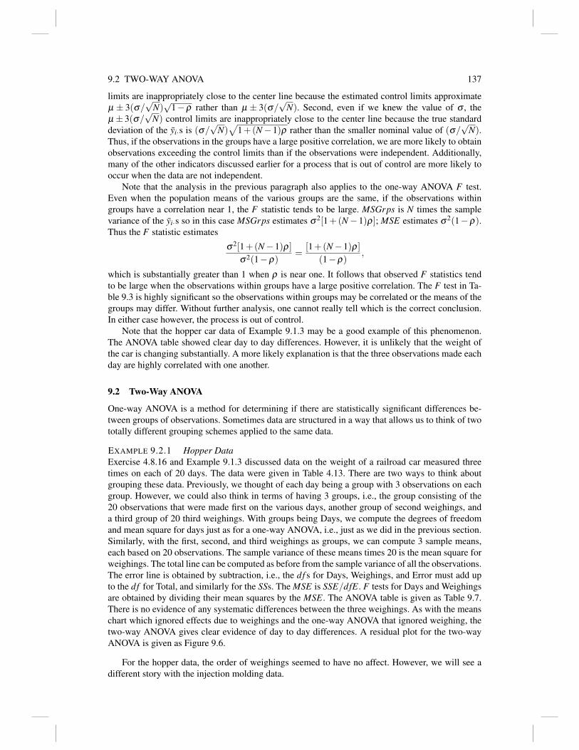
9.2 TWO-WAY ANOVA 137

limits are inappropriately close to the center line because the estimated control limits approximateµ ± 3(σ/

√N)√

1−ρ rather than µ ± 3(σ/√

N). Second, even if we knew the value of σ , theµ ± 3(σ/

√N) control limits are inappropriately close to the center line because the true standard

deviation of the yi·s is (σ/√

N)√

1+(N−1)ρ rather than the smaller nominal value of (σ/√

N).Thus, if the observations in the groups have a large positive correlation, we are more likely to obtainobservations exceeding the control limits than if the observations were independent. Additionally,many of the other indicators discussed earlier for a process that is out of control are more likely tooccur when the data are not independent.

Note that the analysis in the previous paragraph also applies to the one-way ANOVA F test.Even when the population means of the various groups are the same, if the observations withingroups have a correlation near 1, the F statistic tends to be large. MSGrps is N times the samplevariance of the yi·s so in this case MSGrps estimates σ2[1+(N−1)ρ]; MSE estimates σ2(1−ρ).Thus the F statistic estimates

σ2[1+(N−1)ρ]σ2(1−ρ)

=[1+(N−1)ρ]

(1−ρ),

which is substantially greater than 1 when ρ is near one. It follows that observed F statistics tendto be large when the observations within groups have a large positive correlation. The F test in Ta-ble 9.3 is highly significant so the observations within groups may be correlated or the means of thegroups may differ. Without further analysis, one cannot really tell which is the correct conclusion.In either case however, the process is out of control.

Note that the hopper car data of Example 9.1.3 may be a good example of this phenomenon.The ANOVA table showed clear day to day differences. However, it is unlikely that the weight ofthe car is changing substantially. A more likely explanation is that the three observations made eachday are highly correlated with one another.

9.2 Two-Way ANOVA

One-way ANOVA is a method for determining if there are statistically significant differences be-tween groups of observations. Sometimes data are structured in a way that allows us to think of twototally different grouping schemes applied to the same data.

EXAMPLE 9.2.1 Hopper DataExercise 4.8.16 and Example 9.1.3 discussed data on the weight of a railroad car measured threetimes on each of 20 days. The data were given in Table 4.13. There are two ways to think aboutgrouping these data. Previously, we thought of each day being a group with 3 observations on eachgroup. However, we could also think in terms of having 3 groups, i.e., the group consisting of the20 observations that were made first on the various days, another group of second weighings, anda third group of 20 third weighings. With groups being Days, we compute the degrees of freedomand mean square for days just as for a one-way ANOVA, i.e., just as we did in the previous section.Similarly, with the first, second, and third weighings as groups, we can compute 3 sample means,each based on 20 observations. The sample variance of these means times 20 is the mean square forweighings. The total line can be computed as before from the sample variance of all the observations.The error line is obtained by subtraction, i.e., the df s for Days, Weighings, and Error must add upto the df for Total, and similarly for the SSs. The MSE is SSE/dfE. F tests for Days and Weighingsare obtained by dividing their mean squares by the MSE. The ANOVA table is given as Table 9.7.There is no evidence of any systematic differences between the three weighings. As with the meanschart which ignored effects due to weighings and the one-way ANOVA that ignored weighing, thetwo-way ANOVA gives clear evidence of day to day differences. A residual plot for the two-wayANOVA is given as Figure 9.6.

For the hopper data, the order of weighings seemed to have no affect. However, we will see adifferent story with the injection molding data.

138 9. EXPERIMENTAL DESIGN

Table 9.7: Two-Way Analysis of Variance for Hopper Data

Analysis of VarianceSource DF SS MS F PDays 19 296380 15599 18.44 0.000Weighings 2 2049 1024 1.21 0.309Error 38 32147 846Total 59 330576

ehat

- *

40+ * *

- * * * *

- * * * * *

- 2 * * * 2 *

- * * * *

0+ * * * * * * *

- * * * * * * 2

- * * * * * * 2 2 * *

- * *

- * * *

-40+ * * *

-

-

-

- *

-80+

----+---------+---------+---------+---------+---------+--yhat

5900 5950 6000 6050 6100 6150

Figure 9.6: Residual Plot, Hopper data, two factors

EXAMPLE 9.2.2 Injection DataExercise 4.8.16 and Example 9.1.4 examined the outside diameters of injection molded bottles inwhich each sample consisted of the bottles made from the four heads of the injection moldingmachine. The data are in Table 4.15. As in our previous example, there are two ways to group thedata. There are 20 samples each with four observations; the analysis we have used in the past. Butwe can also think of each head providing a group of 20 observations. The 20 samples provide 19degrees of freedom for samples and a mean square based on multiplying the variance of the 20group means by 4. Similarly, the 4 heads provide 3 degrees of freedom for heads and a mean squarebased on multiplying the sample variance of the 4 head means by the number of observations ineach group, 20. The Total line is obtained from the sample variance of all 80 observations. TheError line is obtained by substraction as in the previous example. The ANOVA table is given inTable 9.8. A residual plot is given as Figure 9.7. In Exercise 4.8.16 and Example 9.1.4 in which theheads were ignored, there was no reason to suspect that the process was out of control. However, thisanalysis gives clear evidence that the four heads are giving bottles with different outside diameters(P value of 0.000). In this case, we originally thought that the four heads were providing rationalsubgroups — observations that were being taken under essentially identical conditions. However,the two-way ANOVA shows that the heads are making different kinds of bottles, so they do notprovide essentially identical conditions.

The P value due to Samples in Table 9.6 was a suspiciously high 0.970. The large P value was

9.3 BASIC DESIGNS 139

Table 9.8: Two-Way Analysis of Variance: Injection Data

Analysis of VarianceSource DF SS MS F PSamples 19 0.0216550 0.0011397 1.34 0.194Heads 3 0.1019248 0.0339749 40.03 0.000Error 57 0.0483750 0.0008487Total 79 0.1719548

ehat

- *

- *

.040+ * * *

- * **

- * ** * * * *2 * *

- * * * * *

- * 3* * ** * 2* * *

.000+ * * * * * 2* 2 *

- * ** ** ** * * *

- * * *

- ** * * * * 2

- *

-.040+ * * * ** *

- *

- *

- *

-

----+---------+---------+---------+---------+---------+--yhat

1.960 1.995 2.030 2.065 2.100 2.135

Figure 9.7: Residual Plot, Injection Data, two factors

caused by a problem with the iid model. The heads give different results and those differences wereincorporated into the Error of Table 9.6. In Table 9.7 we separated the previous Error into two parts,one for Heads and a new Error. The new Error is substantially smaller than the old Error becauseit no longer incorporates the Head differences. Missing an important factor like that caused the Fstatistic in Table 9.6 to get unusually small (with an unusually large P value). 2

9.3 Basic Designs

9.3.1 Completely randomized designs

The basic idea of a completely randomized design is that a collection of experimental material isprepared and then experimental treatments are randomly assigned to the material. (Equivalently, thematerial can be randomly assigned to the treatments.) At the beginning of the chapter we discussedan experiment reported by Phillips et al. (1998) that involved tearing pieces of vinyl floor covering.The material to be tested was thoughtfully chosen, carefully prepared, and randomly assigned todifferent machine operators.

The standard analysis for a completely randomized design is a one-way ANOVA with the treat-ments defining the groups. In addition to the experiment discussed above that allows evaluationof the four operators, Phillips et al. (1998) also reported the data of Example 9.1.1 on tear mea-surements for three different types of vinyl floor covering. The background for these data was not

140 9. EXPERIMENTAL DESIGN

reported as carefully as it was for the other data they report. (The data were not as important tothe goal of their article.) But we can presume that it was collected using a completely randomizeddesign, so Example 9.1.1 illustrates the beginning of an analysis for these data. A complete analysisinvolves carefully evaluating the assumptions made in analyzing the data and adjusting the analysisif any of the assumptions seem invalid. A complete analysis would also not end with establishingthat there are differences among the groups. A complete analysis should characterize the differencesamong the groups. In this case, from looking at the group means it is pretty clear that the primarysource of differences between the floor coverings is that Cover B has larger tear values than theother covers. However, statistical methods are often needed to distinguish between patterns in thegroup means that are real and those that are spurious.

9.3.2 Randomized complete block designs

As discussed in the introduction to this chapter, a key method for reducing the variability associatedwith comparing experimental treatments is by creating blocks of homogeneous experimental mate-rial and assigning the treatments to these blocks. A complete block design involves having blocksthat have exactly as many experimental units as there are treatments in the experiment. A random-ized complete block design randomly assigns the treatments to the units within each complete block.(Any time the blocks are not large enough to accommodate all of the treatments, an incomplete blockdesign must be used.)

In the injection molding of Example 9.2.2, if each sample consists of a block of experimentalmaterial and the material were randomly assigned to the four heads, the design would be a random-ized complete block design.

The analysis for a randomized complete block design uses a two-way ANOVA. The treatmentsform one set of groups and the blocks form the other set of groups. For the injection data, the treat-ments are the four heads and blocks are the 20 samples. We saw in the previous section that thereare clear differences between heads but no significant differences between the samples. As in theprevious subsection, a complete analysis of these data involves carefully evaluating the assumptionsmade in analyzing the data and adjusting the analysis if any of the assumptions seem invalid. A com-plete analysis also involves characterizing any differences among the treatment groups. (Differencesamong the blocks are usually of little interest.)

The fundamental idea of blocking is that experimental material within a block should be ho-mogeneous, i.e., the differences in experimental material should be smaller within blocks than theyare between blocks. That is what reduces the error for treatment comparisons. With a random-ized complete block design, the differences between blocks are isolated in the analysis, leaving (ifblocks were created well) a smaller means squared error than would otherwise be obtained. In Ex-ample 9.2.2 we have done a poor job of blocking. The F test for Samples shows that the variabilitybetween blocks is not substantially greater than the variability within blocks. So we have not con-structed blocks that are going to substantially reduce the variability of our treatment comparisons.In fairness to the original authors, we should point out that while the injection data may form areasonable approximation to a randomized complete block design, the data collection was not orig-inally set up as a randomized complete block design, so the fact that samples make poor blocks isnot surprising.

9.3.3 Latin Squares and Greco-Latin Squares

Latin Squares take the idea of randomized complete blocks a step further. In a randomized completeblock, you assign each treatment to some experimental unit in each block. Thus if you pick anyblock, you observe every treatment within it, but also if you pick any treatment, you have an ob-servation with that treatment from every block. There are two ways of grouping the data: by blocksand by treatments.

In a Latin Square design, there are three ways of grouping the data. These are generally referred

9.3 BASIC DESIGNS 141

Table 9.9: 3×3 Latin Square

Columns1 2 3

Rows 1 A B C2 B C A3 C A B

Table 9.10: 3×3 Graeco-Latin Square

Columns1 2 3

Rows 1 Aα Bβ Cγ

2 Bγ Cα Aβ

3 Cβ Aγ Bα

to as rows, columns, and treatments. In a Latin Square, the numbers of rows, columns and treatmentsmust be the same. The key aspect to a Latin Square is that for every row, you observe both everytreatment and every column. For every column, you observe both every treatment and every row.For every treatment, you also observe both every row and every column.

Table 9.9 shows a Latin Square design with three rows and three columns. The treatments aredenoted by Latin letters. Note that each letter appears in each row and in each column.

A Greco-Latin Square involves four ways of grouping the data. These are denoted rows,columns, Latin letters, and Greek letters. Table 9.10 gives a Greco-Latin Square with three rowsand three columns. Note that by ignoring the Greek letters you get a Latin Square in the Latin let-ters. Also by ignoring the Latin letters, you get a Latin Square in the Greek letters. Finally, everyGreek letter appears exactly once with each Latin letter, and vice versa.

EXAMPLE 9.3.1 Byrne and Taguchi (1989) and Lucas (1994) give data on a Greco-Latin Squaredesign. The data are values y which measure the force in pounds needed to pull a plastic tube froma connector. Large values are good. While the information is not of immediate relevance for ourpurposes, the data were collected with a condition time of 24 hours, a condition temperature of72◦F and a condition relative humidity of 25%. There are four grouping factors involved in thedesign: rows (A), columns (B), Latin letters (C), and Greek Letters (D). The actual grouping factorswith their group identifications (levels) are listed below.

A : Interference (a0 =Low, a1 =Medium, a2 =High)B : Wall Thickness (b0 =Thin, b1 =Medium, b2 =Thick)C : Ins. Depth (c0 =Shallow, c1 =Medium, c2 =Deep)D : Percent Adhesive (d0 =Low, d1 =Medium, d2 =High)The actual data are given in Table 9.11.

A partial analysis of variance table is given in Table 9.12. The ANOVA table includes no F testsbecause no MSE can be computed from this design. The sums of squares for factors A, B, C, andD use up all of the Total degrees of freedom and sums of squares. This is a problem that we will

Table 9.11: 3×3 Graeco-Latin Square: Pipe Force Data

b0 b1 b2a0 c0d0 (15.6) c1d1 (18.3) c2d2 (16.4)a1 c1d2 (15.0) c2d0 (19.7) c0d1 (14.2)a2 c2d1 (16.3) c0d2 (16.2) c1d0 (16.1)

142 9. EXPERIMENTAL DESIGN

Table 9.12: Analysis of Variance for Pipe Force Data

Analysis of VarianceSource df SS MSA 2 12.1756 6.0878B 2 0.5489 0.2744C 2 6.8356 3.4178D 2 2.5156 1.2578Error 0 0.0000 —Total 8 22.0756

Table 9.13: L9 Orthogonal Array

AverageRun a b c d Thickness

1 0 0 0 0 15.64 0 1 1 2 18.37 0 2 2 1 16.43 1 0 1 1 15.02 1 1 2 0 19.75 1 2 0 2 14.28 2 0 2 2 16.36 2 1 0 1 16.29 2 2 1 0 16.1

encounter frequently in subsequent chapters. Despite the lack of an Error term and the consequentinability to perform statistical tests, the 4 factors seem to display some substantial differences intheir sums of squares.

Again examining the ANOVA table, note that if there were no factor D, so that this was a 3×3Latin Square with only factors A, B, and C, the ANOVA table line for factor D would actually bean error term. So in a 3× 3 Latin Square we get 2 degrees of freedom for error. Two degrees offreedom for error makes for a very bad estimate of variability, but it is better than nothing. Moreimportantly, two degrees of freedom for error suggest that we could run several similar 3×3 LatinSquares and in the analysis pool the estimates of error, and thus obtain a good estimate of variability,cf. Christensen (1996, Secs. 9.3 and 11.4).

In later chapters Greco-Latin Squares will rear their ugly heads in another guise. Table 9.11 canbe rewritten as Table 9.13. Note that the treatments and data are exactly the same in the two tables.The method of writing a 3×3 Greco-Latin Square used in Table 9.13 is also referred to as a TaguchiL9 orthogonal array.

Below is a further breakdown of the ANOVA table. The left side fits a regression model

yhi jk = β0 +βAh+βBi+βC j+βDk++βA2h2 +βB2i2 +βC2 j2 +βD2k2 + εhi jk.

Notice that adding the two sums of squares for each letter gives the sum of squares presented inTable 9.12. The large sums of squares in Table 9.12 are largely due to one of the two pieces in thistable. If anything is going on in C, it is is pretty much a linear trend over the three levels. If anythingis going on in A it is largely because the middle level is not behaving like the average of the highand low levels.

9.4 FACTORIAL TREATMENT STRUCTURES 143

Table 9.14: Aceves-Mijares et al. 3×3: Graeco-Latin Square.

Columns1 2 3

Rows 1 Aα (0) Bβ (97.9) Cγ (112.8)2 Bγ (3) Cα (208.6) Aβ (104.3)3 Cβ (47.9) Aγ (55.6) Bα (438.7)

b0 b1 b2a0 c0d0 (0) c1d1 (97.9) c2d2 (112.8)a1 c1d2 (3) c2d0 (208.6) c0d1 (104.3)a2 c2d1 (47.9) c0d2 (55.6) c1d0 (438.7)

Table 9.15: Aceves-Mijares et al. (1996): L9 Orthogonal Array.

AverageRun A B C D Thickness

1 0 0 0 0 04 1 0 1 2 37 2 0 2 1 47.93 0 2 2 2 112.82 0 1 1 1 97.95 1 1 2 0 208.68 2 1 0 2 55.66 1 2 0 1 104.39 2 2 1 0 438.7

Regression on yPredictor Coef SEQ SS Predictor SEQ SSβA 4.90000 0.00667 βA 0.007βB −0.649999 0.48167 βB 0.482βC 1.20000 6.82666 βC 6.827βD −1.10000 2.40667 βD 2.407βA2 −2.46667 12.16889 βAB 0.090βB2 0.183333 0.06722 βBC 8.670βC2 −0.0666664 0.00889 βCD 1.562βD2 0.233334 0.10889 βDA 2.032Constant (β0) 15.6000

The right side of the tabulation fits a model

yhi jk = β0 +βAh+βBi+βC j+βDk++βABhi+βBCi j+βCD jk+βDAki+ εhi jk.

For these data, it does not tell as clear a story but note that the sums of squares for A2, B2, C2, andD2 sum to the same total as the sum of squares for AB, BC, CD, and DA and that the results for theconstant, A, B, C, andD are identical (up to roundoff).

9.3.3.1 Additional Example of a Graeco-Latin Square

Aceves-Mijares et al. (1996) give the data in Tables 9.14 and 9.15. The tables provides three alterna-tive methods of denoting the treatments. Aceves-Mijares et al. make no distinction between α andγ , or if you prefer, between d0 and d2.

9.4 Factorial treatment structures

Often, more than one factor is of interest in an experiment. For example, when making a fabric,the wear can be effected by both the surface treatment of the fabric and the type of fill used. When

144 9. EXPERIMENTAL DESIGN

Table 9.16: Surface finish from a lathe.

Speed Feed Finish Speed Feed Finish−1 −1 7 −1 −1 9−1 0 77 −1 0 77−1 1 193 −1 1 190

0 −1 7 0 −1 90 0 75 0 0 800 1 191 0 1 1911 −1 9 1 −1 181 0 79 1 0 801 1 192 1 1 190

Table 9.17: One-Way Analysis of Variance for Surface Finish Data.

Analysis of VarianceSource df SS MS FTreatments 8 100718 1799 223Error 9 64 7Total 17 100782

evaluating waterproofing of a fabric, both the laundry washing the fabric and the laboratory test-ing the fabric may effect results. In evaluating the results of a spectrometer, both the status of thewindow and the status of the boron tip may be important. When more than one factor is of interestin an experiment, there is an effective method for defining treatments, i.e., make the treatments allcombinations of the factors involved. For example, for a spectrometer, the boron tip may be new orused and the window may be clean or soiled. The factorial treatment structure involves 4 treatmentsobtained by crossing the two levels of the tip with the two levels of the window. Thus, the treat-ments are: New-clean, New-soiled, Used-clean, Used-soiled. This is referred to as a 2×2 factorialtreatment structure, where 2×2 = 4 is the number of treatments.

There are two advantages to factorial treatment structures as opposed to running experimentsfor each factor individually. First, running individual experiments may be misleading. If the effectof the boron tip changes depending on whether the window is clean or soiled, you cannot find thatout by running an experiment only on the boron tip. Second, if the effect of the tip does not dependon the window status (and conversely, the effect of the window status does not depend on the borontip), then one experiment using a factorial treatment structure gives as much information on both thetip and the window as does an experiment on the windows and a separate experiment on the borontips.

EXAMPLE 9.4.1 3×3 Factorial.Collins and Collins (1994) report data on the surface finish of a bar that has been lathed. The surfacefinish is measured as the distance a probe moved vertically as it was drawn across the bar horizon-tally. Higher readings indicate rougher surfaces. We can think of this as a completely randomizeddesign with 9 treatments, however the 9 treatments are defined as all combinations of two factorseach having three levels. The first factor is the speed of the lathe with three levels: 2500, 3500, or4500 rpm. The second factor is the rate of feed for the tool with the three levels 0.001, 0.005, and0.009 inches per revolution of the lathe. The data are given in Table 9.16. The one-way ANOVAtable is given as Table 9.17. The F statistic is huge, so there are some differences among the 9treatments.

As discussed earlier in this chapter, examining the ANOVA table is really only the beginning ofa data analysis. A complete analysis involves evaluating assumptions and comparing the treatments.While a detailed examination of such issues is beyond the scope of this book, we now take anintermediate step – we break the line in the ANOVA table for treatments up into components for

9.4 FACTORIAL TREATMENT STRUCTURES 145

Table 9.18: Factorial Analysis of Variance for Surface Finish Data.

Analysis of VarianceSource DF SS MS F Pspeed 2 25 13 1.76 0.227feed 2 100670 50335 7078.38 0.000speed*feed 4 23 6 0.80 0.556Error 9 64 7Total 17 100782

the different factors in the treatment structure. In this case, we have lines for speeds, the feeds,and interactions between the speeds and feeds. Interaction, evaluates whether the effects of speedschanges depending on what feed is being used, or equivalently, it evaluates whether the effects offeeds changes depending on what speed is being used. Table 9.18 gives the expanded ANOVA table.

To compute the expanded ANOVA table, first ignore the feeds altogether. Pretend that this isan experiment with only three treatments: the three speeds. Compute group means for the threespeeds, and perform the usual one-way ANOVA computation, i.e., find the sample variance of thethree speed means and multiply by the number of observations that went into each speed mean. Thisprocess gives the mean square for speeds with 3− 1 = 2 degrees of freedom and a sum of squaresobtained by multiplying the the degrees of freedom and the mean square. A similar computationgives the df , MS, and SS for feeds. Finally, the interaction is that part of the Treatments fromTable 9.17 that is left over after isolating the speed and feed effects. In other words, the interactionsum of squares is obtained by subtracting the speed sum of squares and the feed sum of squaresfrom the sum of squares for treatments. The interaction degrees of freedom are found by a similarsubtraction. F tests in Table 9.18 are computed as the ratio of the means squares for speed, feed, andinteraction divided by the MSE. In evaluating Table 9.18, the first order of business is to examinethe interaction. A significant interaction means that the effects of speeds change depending on whatfeed is used (and that the effect of feeds depend on what speed is used). If there is interaction, theremust be effects for both speeds and feeds. If the effects of speeds change depending on what feedis used then there must be some effect for speeds and if they can change with feeds, the feeds areobviously affecting the results also.

The line in the ANOVA table for speeds examines whether there are speed effects when averag-ing over the feeds used in the experiment. If there is no interaction, the speed effects do not dependon feeds, so this just measures the speed effects. If there is interaction, there really is nothing we cancall speed effects. When there is interaction, speed effects change depending on feeds. Therefore,when there is interaction, looking at speed affects by averaging over the feeds is typically not a veryuseful thing to do. For these data, there is no evidence of interaction so looking as speed effects isreasonable. Similarly, looking at feed effects is only reasonable when there is no interaction. FromTable 9.18, we see no effect for speeds but a substantial effect for feeds. It would be appropriatenow to examine specific comparisons between the results of using the different feeds.

Finally, we should evaluate the assumptions. Figures 9.8 and 9.9 give residual plots for theanalysis. The normal plot looks fine, but the residual plot versus predicted values suggests that thevariances are decreasing with the size of the predicted values. Table 9.19 contains the data, residuals,and fitted values. 2

To conclude we examine a much more challenging experimental design that involves 4 factorseach at 2 levels.

EXAMPLE 9.4.2 24 Factorial.Collins and Collins (1994, qe94-559) also looked at surface finish in another experiment with fourfactors each at two levels. This involved a computer controlled lathe that is fed a bar of stock acertain number of inches per revolution while a tool cuts it. A collet holds the stock in place. The

146 9. EXPERIMENTAL DESIGNehat

- *

-

-

3.0+

- *

-

- 3 *

- *

0.0+ 4

- *

- 3

- *

- *

-3.0+

-

-

- *

+---------+---------+---------+---------+---------+------

-2.10 -1.40 -0.70 0.00 0.70 1.40 rankits

Figure 9.8: Normal Plot of Surface Finish Data

ehat

- *

-

-

3.0+

- *

-

- 2 2

- *

0.0+ 2 2

- *

- 2 *

- *

- *

-3.0+

-

-

- *

+---------+---------+---------+---------+---------+------yhat

0 35 70 105 140 175

Figure 9.9: Residual Plot of Surface Finish Data

four factors and their levels are given in Table 9.20. The data involve two replications of the 16treatments and are given in Table 9.21. Examining the data, there is little need for a formal analysis.y measures roughness and all of the smallest measures are associated with having Feed at 0.003 anda tight Collet. Nonetheless we will use this example to illustrate some tools for analysis.

An ANOVA conducted on the raw data resulted in the residuals versus predicted values plot of

9.4 FACTORIAL TREATMENT STRUCTURES 147

Table 9.19: Residuals and Fitted Values: Surface Finish Data

Case Speed Feed y e y1 −1 −1 7 −1.0 8.02 −1 0 77 0.0 77.03 −1 1 193 1.5 191.54 0 −1 7 −1.0 8.05 0 0 75 −2.5 77.56 0 1 191 0.0 191.07 1 −1 9 −4.5 13.58 1 0 79 −0.5 79.59 1 1 192 1.0 191.0

10 −1 −1 9 1.0 8.011 −1 0 77 0.0 77.012 −1 1 190 −1.5 191.513 0 −1 9 1.0 8.014 0 0 80 2.5 77.515 0 1 191 0.0 191.016 1 −1 18 4.5 13.517 1 0 80 0.5 79.518 1 1 190 −1.0 191.0

Table 9.20: Surface Finish Factors

LevelsFactor −1 1 UnitsSpeed 2500 4500 rpmFeed 0.003 0.009 in./rev.

Collet Loose TightTool Wear New After 250 parts

Figure 9.10. The plot looks like evidence that the variability increases with the mean values, al-though the impression is almost entirely due to the large discrepancy between the two observations273 and 691 corresponding to high speed, low feed, loose collet, and a new tool. As a correctivemeasure we analyzed the reciprocals of the square roots of the data, i.e., 1/

√y. Since y is a mea-

sure of roughness, 1/√

y is a measure of smoothness. A one-way ANOVA for 24 = 16 treatmentson the transformed data results in the much more attractive residual – predicted value plot given

Table 9.21: Surface Finish

Speed Feed Collet Wear Finish Speed Feed Collet Wear Finish1 1 1 1 216 1 1 1 1 217−1 1 1 1 212 −1 1 1 1 221

1 −1 1 1 48 1 −1 1 1 39−1 −1 1 1 40 −1 −1 1 1 31

1 1 −1 1 232 1 1 −1 1 235−1 1 −1 1 248 −1 1 −1 1 238

1 −1 −1 1 514 1 −1 −1 1 437−1 −1 −1 1 298 −1 −1 −1 1 87

1 1 1 −1 238 1 1 1 −1 245−1 1 1 −1 219 −1 1 1 −1 226

1 −1 1 −1 40 1 −1 1 −1 51−1 −1 1 −1 33 −1 −1 1 −1 33

1 1 −1 −1 230 1 1 −1 −1 226−1 1 −1 −1 253 −1 1 −1 −1 214

1 −1 −1 −1 273 1 −1 −1 −1 691−1 −1 −1 −1 101 −1 −1 −1 −1 130

148 9. EXPERIMENTAL DESIGN

Figure 9.10: Residual Plot for ANOVA on y.

Figure 9.11: Residual Plot for ANOVA on 1/sqrt(y).

in Figure 9.11. (We tried several transformations and 1/√

y had the nicest residual plot.) The cor-responding normal plot in Figure 9.12 looks tolerable. It includes too many residuals too close to0.

In the ANOVA of Table 9.22, the 15 degrees of freedom for the 16 treatments have been dividedinto 15 terms. Four are for the average effects of Speed, Feed, Collet, and (Tool) Wear. Six are fortwo factor interactions. For example the Speed*Feed interaction looks at whether the average effectof Speed changed depending on what Feed we are looking at. Another four terms are three fac-tor interactions. For example the Speed*Feed*Collet interaction looks at whether the Speed*Feed

9.4 FACTORIAL TREATMENT STRUCTURES 149

Figure 9.12: Normal Plot for ANOVA on 1/sqrt(y).

Table 9.22: Analysis of Variance for 1/√

y.

Source DF SS MS F PSpeed 1 .0019022 .0019022 14.63 .001Feed 1 .0187102 .0187102 143.86 .000Collet 1 .0179270 .0179270 137.83 .000Wear 1 .0000249 .0000249 0.19 .668Speed*Feed 1 .0018528 .0018528 14.25 .002Speed*Collet 1 .0001504 .0001504 1.16 .298Speed*Wear 1 .0000473 .0000473 0.36 .555Feed*Collet 1 .0168288 .0168288 129.39 .000Feed*Wear 1 .0000437 .0000437 0.34 .570Collet*Wear 1 .0000454 .0000454 0.35 .563Speed*Feed*Collet 1 .0002408 .0002408 1.85 .193Speed*Feed*Wear 1 .0000203 .0000203 0.16 .698Speed*Collet*Wear 1 .0000009 .0000009 0.01 .935Feed*Collet*Wear 1 .0000038 .0000038 0.03 .866Speed*Feed*Collet*Wear 1 .0000002 .0000002 0.00 .967Error 16 .0020810 .0001301Total 31 .0598798

interaction changes between a loose and a tight Collet. Finally, the Speed*Feed*Collet*Wear inter-action looks at whether the Speed*Feed*Collet changes between having a new tool and having aused tool. All of these interaction descriptions remain valid when changing the factors. For example,Speed*Feed is also how the Feed effect changes with Speed, the Speed*Feed*Collet interaction isalso how the Speed*Collet interaction changes depending on the Feed rate, etc. If the four-factorinteraction is important, it means that the three factor interactions must exist and be changing, sothere is no point in looking at average three-factor interaction. If the Speed*Feed*Collet interactionis important then all of the Speed*Feed, Speed*Collet, and Feed*Collet interactions must exist andbe changing. We always investigate the largest interactions first and work our way down. (Down tolower order interactions but physically up the table.)

In these data the primary interaction that looks important is the Feed*Collet interaction but the

150 9. EXPERIMENTAL DESIGN

Speed*Feed interaction also looks significant. With the important interactions being exactly 2 two-factor interactions that share one common term, the simplest method for interpreting the results is tofix the level of the common factor Feed and look at the separate effects of Speed and Collet for eachlevel of Feed. With no missing data we need only look at the Feed-Collet means and the Feed-Speedmeans.

Collet SpeedFeed Loose Tight Feed 2500 45000.003 0.06786 0.16106 0.003 0.12978 0.099140.009 0.06536 0.06683 0.009 0.06620 0.06600

Looking at the Feed-Collet means, it jumps out that the smoothness scores are highest for Feed0.003 and a tight Collet. The other three scores are all comparable so this is the source of the hugeFeed*Collet interaction. Somewhat less obvious is that we can do better at low Speed. From theFeed-Speed means there is little Speed effect at the high Feed rate, but for low Feed, smoothness ishigher at Speed 2500 than at Speed 4500. So our formal analysis found us a worthwhile conclusionabout Speed that was not obvious from the raw data. Although if you go back to the raw data youcan see that among the 8 roughness scores with low Feed and tight Collet, the low Speed scores arealways a little lower than the high Speed scores.

The only effect not involved in the important interactions is Wear and Wear has no obviouseffect. 2

9.5 Exercises

Reanalyze all of the rational subgroup data from the Chapter 4 exercises using one-way ANOVA.

EXERCISE 9.5.1. Reanalyze the hopper car data of Table 4.14 as a two-way ANOVA.

EXERCISE 9.5.2. Reanalyze the injection molding data of Table 4.16 as a two-way ANOVA.

EXERCISE 9.5.3. Schneider and Pruett (1994, qe94-348.dat) look at carbon black DBP valuesover 12 days with 6 readings per day at 3, 7, and 11, both AM and PM (days start at 3PM). The dataare in Table 6.3. Do a time series analysis. Look for day effects and for time within day effects.

EXERCISE 9.5.4. Watch Stuart Hunter’s introduction to Experimental Design: Part 1 and Part 2.

Chapter 10

2n factorials

10.1 Introduction

Often in industrial experimentation there are many factors that need to be explored, accompaniedby high costs for obtaining data and limited budgets. When many factors are involved, the numberof treatments becomes large, so it may be impractical to obtain data on all combinations of thefactors. Even worse, with many treatments it will be impractical to obtain appropriate replicationson the treatments so that a truly valid estimate of the error can be obtained. In such cases, we needmethods for defining appropriate subsets of the treatments so that observations on these treatmentsubsets will provide the information necessary to proceed.

We begin with a number of examples of such problems.

EXAMPLE 10.1.1. Taguchi (1987, qe94-319) and Box and Bisgaard (1994) discuss a study tofind factors that increase the viscosity of sodium silicate. Nine factors were considered.

LevelLabel Factor 0 1A Silica sand type #5 #6B Reaction time 4 hr 5 hrC Agitation 100 150D Reaction temperature 190±3◦C 180±3◦CE Rate of temperature increase 30−35◦C/min 15−20◦C/minF Relative excess of silica sand 20% 10%G Active carbon type T3 3AH Quantity of active carbon 0.13% 0.06%J Evacuated water temperature 80±5◦C 40±5◦C

A factorial experiment would involve 29 = 512 treatments. This is a completely unwieldy number.Instead, it was decided to examine only 16 treatments. With 16 observations, and thus 16 degreesof freedom, 1 df is associated with the grand mean (intercept) and 9 are associated with the maineffects. That leaves 6 degrees of freedom for doing other things. If there is no interaction, the 6degrees of freedom would constitute error. 2

EXAMPLE 10.1.2. Shina (1991) and Lawson and Helps (1996) [q96-467.dat] consider a studyon eight factors that affect a wave-soldering process for printed circuit boards. The factors are A:Preheat Temperature; B: Wave Height; C: Wave Temperature; D: Conv. Angle; E: Flux; F: Direction;G: Wave width. Each factor had two levels being considered so a full factorial involves 28 = 256treatments. Instead, only 32 treatments were examined. 2

EXAMPLE 10.1.3. Sarkar (1997) [qe97-529.dat] examined cleaning efficiencies. The experimentinvolved five factors: feed rate, setting angle, setting distance, feed setting, and opener setting. Afull factorial would involve 25 = 32 treatments. Only 16 treatments were actually run. 2

EXAMPLE 10.1.4. Ferrer and Romero (1995) [qe95-750.dat] examined an experiment designed

151

152 10. 2N FACTORIALS

Table 10.1: Hare’s 1/2 rep. from a 25

Batch Treatment Batch Treatment1 a0b0c0d1e1 9 a0b1c1d1e12 a1b0c1d1e1 10 a1b1c0d1e13 a1b1c0d0e0 11 a0b0c1d1e04 a1b0c1d0e0 12 a0b0c0d0e05 a0b1c0d0e1 13 a1b0c0d0e16 a0b0c1d0e1 14 a1b1c1d0e17 a0b1c0d1e0 15 a1b0c0d1e08 a1b1c1d1e0 16 a0b1c1d0e0

to improve the adhesive force between polyurethane sheets used in inner linings of various equip-ment. The factors involved are A: amount of glue; B: predrying temperature; C: tunnel temperature;D: pressure. Reducing the amount of glue or tunnel temperature can save the manufacturer bigbucks. In this case the full factorial of 24 = 16 treatments were run, but no replication was per-formed. 2

Our primary example follows.

EXAMPLE 10.1.5. Hare (1988) examined data on excessive variability in the taste of a dry soupmix. The source of variability was identified as the ‘intermix’, a component of the overall mixturethat contained flavorful ingredients such as vegetable oil and salt. Five factors were thought to be ofpotential importance. Factor A was the number of ports for adding vegetable oil to the large mixer inwhich intermix is made. This could be either 1 (a0) or 3 (a1). Factor B was the temperature at whichthe mixture was produced. The mixer could be cooled by circulating water through the mixer jacket(b0) or the mixer could be used at room temperature (b1). Factor C was the mixing time: either 60seconds (c0) or 80 seconds (c1). Factor D was the size of the intermix batch: 1500 pounds (d0) or2000 pounds (d1). Factor E was the delay between making the intermix and using it in the final soupmix. The delay could be either 1 day (e0) or 7 days (e1). With 5 factors each at two levels, there are25 = 32 different treatments. For example, one of the treatments is the combination of factor levelsa0b1c0d1e0, i.e., one port, mixing at room temperature, 60 seconds of mixing, 2000 pounds of mix,and using the intermix immediately. In fact, these happen to be the standard operating conditions formaking intermix. Because the experiment is concerned with variability, several observations wereneeded for each treatment so that the variance could be estimated reasonably. As a result, it wasdecided that only 16 of the possible 32 treatments could be considered. Table 10.1 contains a listof the treatments that were actually run. (Standard operating conditions were run in batch 7. Thetreatments were randomly assigned to the batches.) 2

When only 16 of 32 possible treatments are examined, it is referred to as a 1/2 replicate of a 25

design. (25× (1/2) = 16 treatments.) If only 8 of the 32 treatments are examined, the design wouldbe a 1/4 replicate. (25× (1/4) = 8 treatments.) Sometimes these are referred to as 25−1 and 25−2

designs, respectively.In this chapter we present a brief introduction to methods for defining and analyzing appropriate

fractional replications of experiments in which there are f factors each at 2 levels, i.e., 2 f experi-ments. Most of our efforts will be devoted to examining fractional replications that involve n = 2 f−r

observations for some r. Frequently in a 2 f experiment, we will be interested only in estimating thef main effects. To do this one could get by with as little as f + 1 observations. The number ofobservations is the number of degrees of freedom available. One degree of freedom is always asso-ciated with the grand mean (intercept), and there is one degree of freedom necessary for estimatingeach of the main effects. Plackett and Burman (1946) presented designs based on Hadamard matri-ces that allow efficient estimation of main effects. For a Placett-Burman/Hadamard design to exist,

10.2 FRACTIONAL REPLICATION 153

Table 10.2: Two groups obtained from a 25 based on ABCDE

Even Odda0b0c0d0e0 a0b0c0d0e1a0b0c0d1e1 a0b0c0d1e0a0b0c1d0e1 a0b0c1d0e0a0b0c1d1e0 a0b0c1d1e1a0b1c0d0e1 a0b1c0d0e0a0b1c0d1e0 a0b1c0d1e1a0b1c1d0e0 a0b1c1d0e1a0b1c1d1e1 a0b1c1d1e0a1b0c0d0e1 a1b0c0d0e0a1b0c0d1e0 a1b0c0d1e1a1b0c1d0e0 a1b0c1d0e1a1b0c1d1e1 a1b0c1d1e0a1b1c0d0e0 a1b1c0d0e1a1b1c0d1e1 a1b1c0d1e0a1b1c1d0e1 a1b1c1d0e0a1b1c1d1e0 a1b1c1d1e1

the number of observations must be a multiple of 4 but does not need to be a power of 2. MostPlackett-Burman designs are not very good for exploring interactions whereas 2 f−r designs makeit relatively easy to determine what interaction information is available. We will spend consider-able time exploring interactions. A more detailed discussion of these topics is given in Christensen(2017) which includes a modified version of material available in Christensen (1996, Chapter 17).

10.2 Fractional replication

The essence of fractional replication is dividing the 2 f different treatments into equal sized sub-groups (whose sizes are also powers of 2). For a 1/2 replication, we need two groups. The 1/2replication involves obtaining data on only one of the two groups. For a 1/4 replication, we needfour groups. The 1/4 replication involves obtaining data on only one of the four groups. For a 1/8replication, we need eight groups and obtain data on only one of the eight groups. After dividingthe treatments into groups, it does not matter at all which of the groups you actually use, althoughsome authors like Taguchi, for simplicity, have publicized designs based on one particular group.

Of course if we are only looking at half the treatments, we cannot expect to get as much infor-mation as we would if we looked at all of the treatments. Some of the information is going to be lostby using fractional replication. We need to keep track of what things we can and cannot learn froma particular fractional replication. It turns out that many of the effects that we would normally lookat in an analysis of variance are “aliased” with each other. When effects are aliased, you cannot tellthem apart. They are two names for the same thing. So, for example, we might estimate the maineffect for some factor but in a fractional replication it may be impossible to distinguish between thatmain effect and some three factor interaction effect. If we determine that this effect is important,we have no statistical way of determining if it is the main effect that is important or the three factorinteraction that is important. In such a case, the fractional replication will only be useful if we areprepared to assume that the three factor effect cannot be important.

EXAMPLE 10.2.1. Hare (1988) used the standard method for breaking a 25 into two groups. Thetwo groups are given in Table 10.2. Hare used the group on the left. The treatments are listed in adifferent order than in Table 10.1 because in Table 10.1 the treatments are listed in the random orderin which they were actually run.

At this point the simplest way to tell the two groups in Table 10.2 apart is simply by adding allthe subscripts for the treatments. In other words, for the treatment a0b1c0d1e0 we add the numbers

154 10. 2N FACTORIALS

0+ 1+ 0+ 1+ 0 = 2. For all the treatments on the left hand side, the sum is even. For all thetreatments on the right hand side the sum is odd. 2

Different ways of breaking treatments into groups correspond to different patterns of summingsubscripts. The different patterns of summing the subscripts in turn determine different patterns oflost information.

In the Hare example, we created the groups using the sum of all of the subscripts for the treat-ments. By doing so, we lose information on the five factor interaction effect ABCDE. We are usingall of the subscripts so this effect involves all of the factors. The effect ABCDE also determineswhat other information we lose, i.e., it determines the pattern of aliasing. That will be discussedlater in the section on aliasing.

EXAMPLE 10.2.2. Groups for in a 24 experimentConsider now a 24 experiment with factors A, B, C, D each at two levels. We can use the ABCDeffect to break the treatments into two groups.

ABCD FractionsABCD even ABCD odda0b0c0d0 a0b0c0d1a0b0c1d1 a0b0c1d0a0b1c0d1 a0b1c0d0a0b1c1d0 a0b1c1d1a1b0c0d1 a1b0c0d0a1b0c1d0 a1b0c1d1a1b1c0d0 a1b1c0d1a1b1c1d1 a1b1c1d0

On the left the sum of the subscripts for all of the treatments are even, e.g., the sum for treatmenta0b1c1d0 is 0+1+1+0 = 2 which is even. On the right, the sum of the subscripts is always odd.

We can use effects other than ABCD to break the treatments into two groups. If we only wantedtwo groups, it is unlikely that we would use any other effect, but to break things down into morethan two groups it is important to understand this concept. For example, we can use the ABC effectto break the treatments into two groups. In this case, the groups will be determined by the sum ofthe subscripts on only the A, B, and C factors. The groups are

ABC FractionsABC even ABC odda0b0c0d0 a0b0c1d1a0b1c1d0 a0b1c0d1a1b0c1d1 a1b0c0d0a1b1c0d1 a1b1c1d0a0b0c0d1 a0b0c1d0a0b1c1d1 a0b1c0d0a1b0c1d0 a1b0c0d1a1b1c0d0 a1b1c1d1

On the left we have treatments like a0b1c1d0 with 0+1+1 = 2 and on the right we have a0b1c0d1with 0+1+0 = 1. In both cases we have ignored the subscript on d when calculating the sum. Notethat since we are ignoring the d subscript, if we have a0b1c1d0 on the left hand side, we also betterhave a0b1c1d1 on the left.

A final example uses BCD to break up the treatments. The groups are

10.3 ALIASING 155

BCD FractionsBCD even BCD odda0b0c0d0 a0b0c0d1a0b1c1d0 a0b1c1d1a1b0c1d1 a1b0c1d0a1b1c0d1 a1b1c0d0a0b0c1d1 a0b0c1d0a0b1c0d1 a0b1c0d0a1b0c0d0 a1b0c0d1a1b1c1d0 a1b1c1d1

If we want to break the treatments up into four groups, we need to use two defining effects. Forexample, we can cross the groupings for ABC and the groupings for BCD. The table below givesfour groups. Any one of the groups can be used as a 1/4 replicate of a 24 experiment.

ABC, BCD FractionsABC even ABC odd

BCD even BCD odd BCD even BCD odda0b0c0d0 a0b0c0d1 a0b0c1d1 a0b0c1d0a0b1c1d0 a0b1c1d1 a0b1c0d1 a0b1c0d0a1b0c1d1 a1b0c1d0 a1b0c0d0 a1b0c0d1a1b1c0d1 a1b1c0d0 a1b1c1d0 a1b1c1d1

In the first column, the a, b, c subscripts add to an even number and the b, c, d subscripts alsoadd to an even number. In the second column, the a, b, c subscripts add to an even number but theb, c, d subscripts add to an odd number. In the third column, the a, b, c subscripts sum to an odd,and the b, c, d subscripts sum to an even. In the last column, the a, b, c subscripts sum to odd andthe b, c, d subscripts also sum to odd. 2

10.3 Aliasing

As mentioned in the previous section, when we only look at some of the treatment combinations,we loose the ability to tell various treatment effects apart. We can tell which treatments are aliasedwith each other by performing a type of multiplication.

Consider a 1/2 replicate of a 24 in which the groups are determined by the ABCD effect. Tofind aliases for an effect, we multiply the effect by ABCD and drop out any factors that get raisedto an even power. Any factors that get raised to an odd power are just left in the product. Forexample, the effect A is aliased with A×ABCD = A2BCD = BCD. The effect BC is aliased withBC× ABCD = AB2C2D = AD. The effect BCD is aliased with BCD× ABCD = AB2C2D2 = A.Oops, we already knew that!

The entire aliasing structure is given below.Effect ×ABCD AliasA = BCDB = ACDC = ABDD = ABCAB = CDAC = BDBC = ADAD = BCBD = ACCD = ABABC = DABD = CACD = BBCD = AABCD —

156 10. 2N FACTORIALS

Table 10.3: Aliases for a 1/2 rep. from a 25 based on ABCDE

Effect ×ABCDE AliasA = BCDEB = ACDEC = ABDED = ABCEE = ABCD

AB = CDEAC = BDEAD = BCEAE = BCDBC = ADEBD = ACEBE = ACDCD = ABECE = ABDDE = ABC

If we consider the 1/2 replicate of a 24 with groups determined by BCD, the aliasing structureis given below.

Effect ×BCD AliasA = ABCDB = CDC = BDD = BCAB = ACDAC = ABDBC = ADAD = ABCBD = CCD = BABC = ADABD = ACACD = ABBCD —ABCD = A

For example ABC×BCD = AB2C2D = AD.Table 10.3 gives the aliases that apply to Hare’s experiment.When we create more than two groups in order to get something smaller than a 1/2 replicate,

the aliasing structure becomes more involved. Consider again the groups formed by ABC and BCDin a 24. The aliases involve both of these defining effects as well as another effect. For a 1/4threplicate, we need 4 groups so there is going to be 4− 1 = 3 effects involved in aliasing. If we doa 1/8 replication, this involves creating 8 groups, so there would be 8− 1 = 7 effects involved inaliasing. We need to be able to identify these other effects. With ABC and BCD defining groups, theother effect is ABC×BCD = AB2C2D = AD. To see that this makes some sense, observe that wewould get the same four groups if we used, say, ABC and AD to define the groups rather than ABCand BCD. As illustrated earlier, with ABC and BCD defining groups, the groups of treatments areas given below.

ABC even ABC oddBCD even BCD odd BCD even BCD odda0b0c0d0 a0b0c0d1 a0b0c1d1 a0b0c1d0a0b1c1d0 a0b1c1d1 a0b1c0d1 a0b1c0d0a1b0c1d1 a1b0c1d0 a1b0c0d0 a1b0c0d1a1b1c0d1 a1b1c0d0 a1b1c1d0 a1b1c1d1

10.3 ALIASING 157

With ABC and AD defining the groups we get the same four groups.

ABC even ABC oddAD even AD odd AD odd AD evena0b0c0d0 a0b0c0d1 a0b0c1d1 a0b0c1d0a0b1c1d0 a0b1c1d1 a0b1c0d1 a0b1c0d0a1b0c1d1 a1b0c1d0 a1b0c0d0 a1b0c0d1a1b1c0d1 a1b1c0d0 a1b1c1d0 a1b1c1d1

We would also get the same four groups if we used AD and BCD to define the groups.In terms of finding the aliases, the 1/4 replication of a 24 involves collecting data on only four

treatments, so there are only 4− 1 = 3 effects that can really be estimated. To find these, multiplyeach effect by all three of the defining effects, ABC, BCD, and AD.

A × ABC = A2BC = BC,

A × BCD = ABCD,

A × AD = A2D = D,

soA = BC = ABCD = D.

Similarly,B = AC =CD = ABD

andC = AB = BD = ACD.

EXAMPLE 10.3.3. 1/8 replication of a 28 experimentThe 28 experiment involves eight factors, call them A through H. A 1/8th replication of the 28 = 256treatments involves only 32 treatments. The 1/8 = 2−3 replication involves specifying 3 definingeffects, say ABCD, EFGH, and CDEF but with 8 groups there are really 8−1 = 7 effects involvedin aliasing. Multiplying pairs of these defining effects and also multiplying all three of the effectstogether give the 4 other effects that implicitly define the 1/8 replication. These other implicitdefining effects are ABEF , CDGH, ABCDEFGH, and ABGH. For example,

ABCD×EFGH = ABCDEFGH.

To find the alias of an effect, multiply the effect by all 7 of these aliasing effects. For A thealiases are

A = A(ABCD) = A(EFGH) = A(CDEF) = A(ABED)

= A(CDGH) = A(ABCDEFGH) = A(ABGH).

Simplifying gives

A = BCD = AEFGH = ACDEF = BED = ACDGH = BCDEFGH = BGH.

The two-factor effect AB has aliases

AB = AB(ABCD) = AB(EFGH) = AB(CDEF) = AB(ABED)

= AB(CDGH) = AB(ABCDEFGH) = AB(ABGH)

which upon simplification become

AB =CD = ABEFGH = ABCDEF = ED = ABCDGH =CDEFGH = GH.

158 10. 2N FACTORIALS

Table 10.4: Hare’s 1/2 rep. from a 25 based on ABCDE

Batch Treatment sc sp1 a0b0c0d1e1 0.43 0.782 a1b0c1d1e1 0.52 1.103 a1b1c0d0e0 0.58 1.704 a1b0c1d0e0 0.55 1.285 a0b1c0d0e1 0.58 0.976 a0b0c1d0e1 0.60 1.477 a0b1c0d1e0 1.04 1.858 a1b1c1d1e0 0.53 2.109 a0b1c1d1e1 0.38 0.76

10 a1b1c0d1e1 0.41 0.6211 a0b0c1d1e0 0.66 1.0912 a0b0c0d0e0 0.55 1.1313 a1b0c0d0e1 0.65 1.2514 a1b1c1d0e1 0.72 0.9815 a1b0c0d1e0 0.48 1.3616 a0b1c1d0e0 0.68 1.18

10.4 Analysis Methods

One new problem we have when fitting ANOVA or other models to fractional replications is thatthere is no natural estimate of error because there is no replication. We don’t even have observationson every factor combination, much less multiple observations on treatments. We present two waysto proceed. One is to assume that higher-order interactions do not exist and use them to estimate theerror. The other is based on a graphical display of the effects that is similar in spirit to a normal plot.

EXAMPLE 10.4.1. Consider again the 1/2 rep. of a 25 from Hare (1988). The experimentalbackground was discussed in Example 10.1.5. The two 1/2 rep. treatment groups were given inTable 10.2 and the aliasing structure was given in Table 10.3. The issue is excessive variability inthe taste of a dry soup mix due to the ‘intermix’ containing flavorful ingredients such as salt andvegetable oil. For each intermix batch (treatment combination), the original data are groups of 5samples taken every 15 minutes throughout a day of processing. Thus each batch yields data fora balanced one-way analysis of variance with N = 5. The data actually analyzed are derived fromthe ANOVAs on different batches. There are two sources of variability in the original observations,the variability within a group of 5 samples and variability that occurs between 15 minute intervals.From the analysis of variance data, the within group variability is estimated with the MSE andsummarized as the estimated ‘capability’ standard deviation

sc =√

MSE.

The ‘process’ standard deviation was defined as the standard deviation of an individual observation.The standard deviation of an observation incorporates both the between group and the within groupsources of variability. Based on a one-way ANOVA model in which the group means are consideredrandom, the estimated process standard deviation is taken as

sp =

√MSE +

MSGrps−MSE5

,

where the 5 is the number of samples taken at each time. These two statistics, sc and sp, are availablefrom every batch of soup mix prepared and provide the data for analyzing batches. The 1/2 rep. ofa 25 specifies different ways of making batches of soup mix. The design and the standard deviationsare given in Table 10.4. For now, we analyze only the data on sp.

This is a “resolution V” (V is a Roman numeral) design because the only defining effect for

10.4 ANALYSIS METHODS 159

Table 10.5: ANOVA for Hare’s sp

Source Source df SS RankA A 1 0.0841 10B B 1 0.0306 7C C 1 0.0056 4D D 1 0.0056 3AB AB 1 0.0009 1AC AC 1 0.0361 8AD AD 1 0.0036 2BC BC 1 0.0182 5BD BD 1 0.1056 12CD CD 1 0.0210 6ABC DE 1 0.3969 13ABD CE 1 0.0729 9ACD BE 1 0.6561 14BCD AE 1 0.0930 11ABCD E 1 0.8836 15Total Total 15 2.4140

the fractional replication is a 5-factor interaction. Given our methods for finding aliases, all maineffects are confounded with four-factor interactions and all two-factor interactions are confoundedwith three-factor interactions. If we are prepared to assume that there are no three- or four-factor in-teractions, we have available estimates of all the main effects and two-factor interactions. Table 10.5contains an ANOVA table with two columns labeled ‘Source.’ The first does not involve factor E andthe second replaces high-order interactions not involving E with their lower order aliases. Table 10.5also contains a ranking of the sizes of the sums of squares from smallest to largest.

The reason for having two Source columns in Table 10.5 is that many ANOVA computer pro-grams will not fit fractional factorials. If you are stuck with such a program, the simplest way toobtain an analysis is to trick it into doing most of the work. If we could drop one of our factors,our 1/2 rep. would become a full factorial (without replication) on the remaining factors. For exam-ple, if we dropped factor E, and thus dropped the e terms from all the treatment combinations inTable 10.4, we would have observations on all 16 of the treatment combinations in the 24 definedby A, B, C, and D. It is easy to find computer programs that will analyze a full factorial. Table 10.5gives the results of an analysis in which we ignored the presence of factor E. The first column ofTable 10.5 contains the sources from the full factorial on A, B, C, and D; the second column replacesthe higher order interactions from the full factorial with their lower order aliases. In computing thefull factorial one might also have to drop the four-factor interaction from the model so that theprogram can relabel it as a one degree of freedom Error term.

The simpler, but more dangerous, method of analysis is to assume that no higher order inter-actions exist and form an error term by pooling the estimable terms that involve only higher orderinteractions. A particular term involves only higher order interactions if the term and all of its aliasesare high order interactions. What we mean by high order interactions is intentionally left ill definedto maintain flexibility. In this design, unless you consider second-order interactions as higher order,there are no terms involving only higher order interactions. Most often, higher order interactions aretaken to be interactions that only involve three or more factors, but in designs like this, one mightbe willing to consider two-factor interactions as higher order to obtain an error term for testingmain effects. (I personally would not be willing to do it with these data.) Often terms that involveonly three and higher order interactions are pooled into an error, but in designs with more factorsand many high order interactions, one might wish to estimate three-factor interactions and use onlyterms involving four or more factors in a pooled error.

If we assume away all two-factor and higher order interactions for the present data, the ANOVAtable becomes that displayed in Table 10.6. With this error term, only factor E appears to be impor-tant. As we will see later, most of the important effects in these data seem to be interactions, so the

160 10. 2N FACTORIALS

Table 10.6: Analysis of variance on sp for Hare’s data

Source d f SS MS FA 1 0.0841 0.0841 0.60B 1 0.0306 0.0306 0.22C 1 0.0056 0.0056 0.04D 1 0.0056 0.0056 0.04E 1 0.8836 0.8836 6.29Error 10 1.4044 0.1404Total 15 2.4140

error term based on no interactions is probably inappropriate. That is why we referred to this as thesimpler but more dangerous method. 2

Graphical methods of analysis are similar to normal plots and are based on plotting ordered(ranked) sums of squares. In a normal plot, the data from a single sample are ordered from smallestto largest and plotted against the expected order statistics from a standard normal distribution. Inother words, the smallest observation in a sample of size, say, 13 is plotted against the expectedvalue for the smallest observation in a sample of size 13 from a N(0,1) distribution. The secondsmallest observation is plotted against the expected value for the second smallest observation in asample of size 13 from a N(0,1) distribution, and so on. This plot should approximate a straight lineif the data are truly normal, the slope of the plot estimates the standard deviation of the population,and the intercept estimates the population mean.

The graphical display presented here is a χ2(1) plot. In general, find the sums of squares forthe various factors in the 2 f−r experiment and denote them SS j. If there are no effects in the exper-iment, every SS j should have a χ2(1) distribution multiplied by σ2. Any term that corresponds toa substantial effect should be larger than a σ2 χ2(1) distribution. Order the sums of squares fromsmallest to largest denoted SS( j). We are going to plot these order statistics against the expectedvalues of the order statistics from a χ2(1) distribution. If there are no effects in the experiment, thisshould give a rough straight line (with slope σ2). Large effects should be visible in that they shouldcorrespond to the largest order statistics and should jump up from the straight line created by theplot of the smaller expected order statistics against the smaller observed order statistics. It is difficultto find the expected order statistics but they are easy to approximate. If F is the the cdf for the χ2(1)distribution, the expected value of the jth order statistic is approximately F−1[ j/(n+1)]. Thus weplot the pairs

(F−1[ j/(n+1)],SS( j)

), looking for a linear relationship for the smaller values and

with upward jumps from the linear relationship identifying important effects.A more common method than to use χ2(1) plots is to use half-normal plots of the positive

square roots of the sums of squares. To construct half-normal plots requires the cdf for the half-normal distribution which is p = 2Φ(x)− 1 for x > 0. Here Φ is the cdf of a standard normaldistribution. The inverse of the half-normal cdf is x = Φ−1

(p+1

2

). The half normal plot is of the

pairs(

Φ−1[

p j+12

],√

SS( j)

)where, by analogy with the χ2(1) plot, we would use p j = j/(n+1),

but more commonly one takes p j = ( j− 0.5)/n. Again, this should be a rough straight line withimportant effects jumping up from the line on the right side.

EXAMPLE 10.4.1 CONTINUED. From the ranked sums of squares in Table 10.5 and the formulafor computing approximate χ2(1) scores, we construct Table 10.7 containing the scores and theordered sums of squares necessary for the χ2(1) plot of the 15 effects from Hare’s data. Figure 10.1contains the plot. Again, the χ2(1) scores in Table 10.13 are approximate expected order statistics.They are computed by applying the inverse of the χ2(1) cumulative distribution function to thevalues j/(n+1), where j goes from 1 to 15 and n = 15.

The key to the graphical analysis is that nonnegligible treatment effects cause the sums of

10.4 ANALYSIS METHODS 161

Table 10.7: χ2(1) scores and ordered sums of squares for Hare’s (1988) data.

χ2(1) Orderedscores SS

0.00615 0.00090.02475 0.00360.07711 0.00560.07711 0.00560.16181 0.01820.23890 0.02100.33539 0.03060.45494 0.03610.60283 0.07290.78703 0.08411.02008 0.09301.32330 0.10561.73715 0.39692.35353 0.65613.46977 0.8836

SS

0.90+ *

-

-

-

- *

0.60+

-

-

- *

-

0.30+

-

-

- * *

- ** * *

0.00+ 22**

-

--+---------+---------+---------+---------+---------+----

0.00 0.70 1.40 2.10 2.80 3.50

Scores

Figure 10.1: χ2(1) plot of sums of squares.

squares to estimate something larger than σ2. The sums of squares for nonnegligible effects shouldshow up in the plot as inappropriately large values. The lower 12 observations in Figure 10.1 seemto fit roughly on a line, but the three largest observations seem to be inconsistent with the others.These three observations correspond to the most important effects in the data. From the rankings inTable 10.5, we see that the important effects are E, BE, and DE.

We need to evaluate the meaning of the important effects. The largest effect is due to E, thedelay in using the intermix. However, this effect is complicated by interactions involving the delay.To evaluate the BE interaction we need the means for the four combinations of B and E.

162 10. 2N FACTORIALS

BE b0 b1e0 1.215 1.7075e1 1.150 0.8325

The BE interaction is due to the fact that running the mixer at room temperature, b1, increasesvariability if the intermix is used after one day, e0, but decreases variability if the intermix is used aweek later, e1. However, the variability under delay is smaller for both B levels than the variabilityfor immediate use with either B level. This suggests delaying use of the intermix.

To evaluate the DE interaction we need the means for the four combinations of D and E.

DE d0 d1e0 1.3225 1.6000e1 1.1675 0.8150

A large batch weight, d1, causes increased variability when the intermix is used immediately butdecreased variability when use is delayed to 7 days. Again, it is uniformly better to delay.

Overall, the best combination of treatments involve e1, b1 and d1. Recalling that the currentprocess is batch 7 with one vegetable oil port, room temperature mixing, 60 seconds mixing time,2000 pound batches, and a 1 day delay, we would recommend changing to a 7 day delay becausethat minimizes process variability. As alluded to in the next chapter, if this change for the purposeof reducing process variability puts the process off target, it might be possible to use factors A andC to put it back on target, since A and C do not seem to affect process variability. 2

Christensen (1996, Sections 17.3 and 17.4) expands on this graphical analysis.

Minitab commands

Below are given Minitab commands for obtaining the analysis given. The data file had eightcolumns, the first six were indicators for batch and factors A, B, C, D and E, respectively. Columns7 and 8 contained the data on sc and sp.

names c8 ’y’ c2 ’a’ c3 ’b’ c4 ’c’ c5 ’d’ c6 ’e’

anova c8=c2|c3|c4|c5 - c2*c3*c4*c5

note AFTER SEEING THE ANOVA, ENTER THE SUMS

note OF SQUARES INTO c10.

set c10

841 306 56 56 9 361 36 182

1056 210 3969 729 6561 930 8836

end

let c10=c10/10000

note CONSTRUCT CHI-SQUARED SCORES AND PLOT.

rank c10 c11

let c11=c11/16

invcdf c11 c12;

chisquare 1.

plot c10 c12

Note that c6 was not used in the anova command. Factor E was dropped to deal with the fractionalnature of the factorial. Minitab’s ANOVA command requires an error term to exist in the model.The command given above specifies a full factorial model (c2|c3|c4|c5) but subtracts out the ABCD

10.5 ALTERNATIVE FORMS OF IDENTIFYING TREATMENTS 163

Table 10.8: Alternative forms of identifying treatments: subscripts only and only letters with subscript 1.

Treatment NotationTreatment Subscripts only Letters with 1. Yield

a0b0c0d0e0 f0g0h0 j0 000000000 −−− 17a1b0c0d0e0 f1g1h1 j1 100001111 a f gh j 21a0b1c0d0e1 f0g1h1 j1 010010111 begh j 41a1b1c0d0e1 f1g0h0 j0 110011000 abe f 20a0b0c1d0e1 f1g0h0 j1 001011001 ce f j 10a1b0c1d0e1 f0g1h1 j0 101010110 acegh 42a0b1c1d0e0 f1g1h1 j0 011001110 bc f gh 14a1b1c1d0e0 f0g0h0 j1 111000001 abc j 58a0b0c0d1e1 f1g0h1 j0 000111010 de f h 8a1b0c0d1e1 f0g1h0 j1 100110101 adeg j 18a0b1c0d1e0 f1g1h0 j1 010101101 bd f g j 7a1b1c0d1e0 f0g0h1 j0 110100010 abdh 15a0b0c1d1e0 f0g0h1 j1 001100011 cdh j 8a1b0c1d1e0 f1g1h0 j0 101101100 acd f g 10a0b1c1d1e1 f0g1h0 j0 011110100 bcdeg 12a1b1c1d1e1 f1g0h1 j1 111111011 abcde f gh j 10

interaction (c2 ∗ c3 ∗ c4 ∗ c5) and sets it equal to the error. Thus, Minitab’s error term is actuallythe ABCD interaction. The command ‘set c10’ is used to create a data column that contains thesums of squares for the various effects. The commands involving c11 and c12 are used to get theapproximate expected order statistics from a χ2(1) and to plot the ordered sums of squares againstthe expected order statistics. After identifying the important effects, the ANOVA command can berepeated with various factors deleted to obtain the necessary means tables.

10.5 Alternative forms of identifying treatments

In this chapter we have used the subscripts 0 and 1 to indicate the levels of treatments. Alterna-tive notations are extremely common and must be recognized. Tables 10.4 through 10.6 providesome alternative notations for the 16 treatments actually used in the viscosity experiment of Exam-ple 10.1.1. Table 10.4 provides two alternatives and the actual data. The first alternative relies onthe fact that if you know the order of the factors, all you really need are the subscript values. Thesecond alternative only reports the letters with the subscript 1. Table 10.5 replaces the subscript 0with −1 and reports only the subscripts. Here we have explicitly written 1 as +1, but the + sign isirrelevant! The notation using −1 and 1 is quite common, is particularly useful for response surfacedesigns, and is employed in Table 11.4. Table 9.21 also used the −1 and 1 notation and Tables 9.16and 9.19 used −1, 0, 1 to denote three levels of a factor. Table 10.6 replaces −1 and +1 with − and+.

10.6 Placket-Burman Designs

When looking at 2 f designs, a generalization of looking at 2 f−r fractional factorials is the use ofPlacket-Burman designs. They are based on Hadamard matrices and exist for some run sizes that aremultiples of n = 4. These include n = 4,8,12,16,20. Designs with n = 12,20 are not powers of 2,so they add flexibility to the choice of designs beyond the 2 f−r fractional designs. For example youcan estimate main effects for 9, 10, or 11 factors in 12 runs with a Placket-Burman design whereasthe smallest 2 f−r design involves 16 = 29−5 = 210−6 = 211−7 different runs. TiD contains moreinformation on Placket-Burman designs.

164 10. 2N FACTORIALS

Table 10.9: Alternative forms of identifying treatments: subscripts only, 1,0 replaced with ±1.

Treatment A B C D E F G H Ja0b0c0d0e0 f0g0h0 j0 −1 −1 −1 −1 −1 −1 −1 −1 −1a1b0c0d0e0 f1g1h1 j1 +1 −1 −1 −1 −1 +1 +1 +1 +1a0b1c0d0e1 f0g1h1 j1 −1 +1 −1 −1 +1 −1 +1 +1 +1a1b1c0d0e1 f1g0h0 j0 +1 +1 −1 −1 +1 +1 −1 −1 −1a0b0c1d0e1 f1g0h0 j1 −1 −1 +1 −1 +1 +1 −1 −1 +1a1b0c1d0e1 f0g1h1 j0 +1 −1 +1 −1 +1 −1 +1 +1 −1a0b1c1d0e0 f1g1h1 j0 −1 +1 +1 −1 −1 +1 +1 +1 −1a1b1c1d0e0 f0g0h0 j1 +1 +1 +1 −1 −1 −1 −1 −1 +1a0b0c0d1e1 f1g0h1 j0 −1 −1 −1 +1 +1 +1 −1 +1 −1a1b0c0d1e1 f0g1h0 j1 +1 −1 −1 +1 +1 −1 +1 −1 +1a0b1c0d1e0 f1g1h0 j1 −1 +1 −1 +1 −1 +1 +1 −1 +1a1b1c0d1e0 f0g0h1 j0 +1 +1 −1 +1 −1 −1 −1 +1 −1a0b0c1d1e0 f0g0h1 j1 −1 −1 +1 +1 −1 −1 −1 +1 +1a1b0c1d1e0 f1g1h0 j0 +1 −1 +1 +1 −1 +1 +1 −1 −1a0b1c1d1e1 f0g1h0 j0 −1 +1 +1 +1 +1 −1 +1 −1 −1a1b1c1d1e1 f1g0h1 j1 +1 +1 +1 +1 +1 +1 −1 +1 +1

Table 10.10: Alternative forms of identifying treatments: subscripts only, 0,1 replaced with −, +.

Treatment A B C D E F G H Ja0b0c0d0e0 f0g0h0 j0 − − − − − − − − −a1b0c0d0e0 f1g1h1 j1 + − − − − + + + +a0b1c0d0e1 f0g1h1 j1 − + − − + − + + +a1b1c0d0e1 f1g0h0 j0 + + − − + + − − −a0b0c1d0e1 f1g0h0 j1 − − + − + + − − +a1b0c1d0e1 f0g1h1 j0 + − + − + − + + −a0b1c1d0e0 f1g1h1 j0 − + + − − + + + −a1b1c1d0e0 f0g0h0 j1 + + + − − − − − +a0b0c0d1e1 f1g0h1 j0 − − − + + + − + −a1b0c0d1e1 f0g1h0 j1 + − − + + − + − +a0b1c0d1e0 f1g1h0 j1 − + − + − + + − +a1b1c0d1e0 f0g0h1 j0 + + − + − − − + −a0b0c1d1e0 f0g0h1 j1 − − + + − − − + +a1b0c1d1e0 f1g1h0 j0 + − + + − + + − −a0b1c1d1e1 f0g1h0 j0 − + + + + − + − −a1b1c1d1e1 f1g0h1 j1 + + + + + + − + +

10.7 Exercises

EXERCISE 10.7.1. In Example 10.1.1. we introduced the viscosity example of Taguchi (1987)and Box and Bisgaard (1994). The 16 treatments were obtained by using the defining effects

BCDE, ABG, ABCJ, ABDH, ABEF.

(These are hard to guess but easy to check.) Note that with 9 factors and 5 defining effects, thenumber of treatments being examined is 16 = 24 = 29/25 = 29−5. The aliasing structure here isvery complicated because in addition to the 5 defining effects, there are 26 other effects involved inthe aliasing. There are 5 =

(51

)original defining effects, 10 =

(52

)effects obtained by multiplying

pairs of the defining effects, 10 =(5

3

)obtained by multiplying triples of the defining effects, 5 =

(54

)obtained by multiplying groups of 4 defining effects, and 1 =

(55

)effect obtained by multiplying

together all five defining effects. The actual treatments and data are given in Table 10.4. Afterevaluating a residual analysis on a reduced model for the untransformed data, Box and Bisgaard(1994) suggest taking logs of the data.

10.7 EXERCISES 165

Table 10.11: Wave soldering.

treatment subscriptsCase a b c d e f g h Yellow

1 0 0 0 0 0 0 0 0 6.002 1 0 0 0 0 0 1 1 10.003 0 1 0 0 0 0 0 1 10.004 1 1 0 0 0 0 1 0 8.505 0 0 1 0 0 1 0 1 1.506 1 0 1 0 0 1 1 0 0.257 0 1 1 0 0 1 0 0 1.758 1 1 1 0 0 1 1 1 4.259 0 0 0 1 0 1 1 1 6.50

10 1 0 0 1 0 1 0 0 0.7511 0 1 0 1 0 1 1 0 3.5012 1 1 0 1 0 1 0 1 3.2513 0 0 1 1 0 0 1 0 6.0014 1 0 1 1 0 0 0 1 9.5015 0 1 1 1 0 0 1 1 6.2516 1 1 1 1 0 0 0 0 6.7517 0 0 0 0 1 0 0 0 20.0018 1 0 0 0 1 0 1 1 16.5019 0 1 0 0 1 0 0 1 17.2520 1 1 0 0 1 0 1 0 19.5021 0 0 1 0 1 1 0 1 9.6722 1 0 1 0 1 1 1 0 2.0023 0 1 1 0 1 1 0 0 5.6724 1 1 1 0 1 1 1 1 3.7525 0 0 0 1 1 1 1 1 6.0026 1 0 0 1 1 1 0 0 7.3027 0 1 0 1 1 1 1 0 8.7028 1 1 0 1 1 1 0 1 9.0029 0 0 1 1 1 0 1 0 19.3030 1 0 1 1 1 0 0 1 26.7031 0 1 1 1 1 0 1 1 17.7032 1 1 1 1 1 0 0 0 10.30

EXERCISE 10.7.2. In Example 10.1.2. we introduced the Shina (1991) and Lawson and Helps(1996) [q96-467.dat] experiment on wave-soldering with 8 factors but only 32 = 28−3 observations.The effects involved in aliasing are

ABFH, ACFG, ADG, BCGH, BDFGH, CDF, ABCDH.

The first three are defining effects. The actual design and data are given in Table 10.7. Yellow is thedependent variable.

EXERCISE 10.7.3. In Example 10.1.3. we introduced Sarkar’s (1997) [qe97-529.dat] 25−1 ex-periment on cleaning efficiencies with five factors but only 16 observations. Tables 10.8 and 10.9give the design and the data, respectively.

Do you find the number of identical data values disturbing? Are there two dependent variables?Why are there 4 replications? Are they studying variability?

EXERCISE 10.7.4. In Example 10.1.4 we considered an unreplicated 24 design given in Ferrerand Romero (1995) [qe95-750.dat] for the improvement of adhesive force between polyurethanesheets. The design and data are given in Table 10.10. Use these data to illustrate the method ofanalysis for experiments that do not involve replications.

EXERCISE 10.7.5. Chapman (1996) data from qe96-35.dat in Table 10.11. Photographic color

166 10. 2N FACTORIALS

Table 10.12: Sarkar’s design.

ERM MCO MCO ERM ERMFeed Setting Setting Feed OpenerRate Angle Distance Setting Setting

Trial a b c d e1 40 6 5 4.5 42 40 6 5 3 33 40 6 4 4.5 34 40 6 4 3 45 40 10 5 4.5 36 40 10 5 3 47 40 10 4 4.5 48 40 10 4 3 39 72 6 5 4.5 3

10 72 6 5 3 411 72 6 4 4.5 412 72 6 4 3 313 72 10 5 4.5 414 72 10 5 3 315 72 10 4 4.5 316 72 10 4 3 4

Table 10.13: Sarkar’s data.

Cleaning EfficiencyAfter ERM Opener Overall

Trial 1 2 3 4 1 2 3 41 35.99 38.33 38.72 39.89 51.20 51.20 52.38 51.992 38.33 39.11 39.89 38.72 50.81 50.42 51.20 50.813 39.89 39.42 39.11 38.72 51.20 50.81 50.81 50.424 38.72 38.72 39.11 39.42 51.20 50.81 50.81 50.425 39.89 39.89 39.11 39.42 51.20 50.81 50.81 50.426 39.42 39.42 39.11 38.72 51.20 50.20 50.81 50.427 40.28 39.11 39.11 38.72 51.20 50.81 50.81 50.428 39.11 39.11 39.42 39.21 51.20 51.20 50.81 50.819 55.06 55.06 50.30 52.30 56.35 58.08 57.64 56.78

10 55.06 54.19 53.76 52.46 57.22 57.22 56.78 56.7811 55.92 55.49 55.49 53.76 57.64 57.64 57.22 56.7812 54.19 53.76 53.76 53.33 57.22 56.35 56.68 55.9213 55.92 55.06 54.62 54.19 58.08 57.64 57.22 56.3514 55.06 54.62 54.62 54.19 57.64 57.64 57.22 57.7815 54.62 54.62 54.19 54.19 57.22 57.78 57.78 55.9216 54.62 54.19 54.19 53.76 56.78 56.35 56.35 55.92

slide development. Responses refer to levels of Red, Green, and Blue. Design variables are 6 devel-oper constituents.

EXERCISE 10.7.7. Anand (1994) data from qe94-39.dat in Table 10.12.

10.7 EXERCISES 167

Table 10.14: Ferrer and Romero’s adhesive force data.

treatment subscripts AdhesiveCase a b c d Force

1 0 0 0 0 3.802 1 0 0 0 4.343 0 1 0 0 3.544 1 1 0 0 4.595 0 0 1 0 3.956 1 0 1 0 4.837 0 1 1 0 4.868 1 1 1 0 5.289 0 0 0 1 3.29

10 1 0 0 1 2.8211 0 1 0 1 4.5912 1 1 0 1 4.6813 0 0 1 1 2.7314 1 0 1 1 4.3115 0 1 1 1 5.1616 1 1 1 1 6.06

Table 10.15: Chapman’s screening experiment for 12 variables

D1 D2 D3 D4 D5 D6 Rmx Gmx Bmx Rhd Ghd Bhd1.5 2.1 7 .2 6.8 9.75 4 −8 −5 −1 0 −37.0 2.1 7 .1 3.5 9.75 −4 −17 −21 −6 −10 −131.5 3.6 7 .1 6.8 9.55 11 2 7 11 11 87.0 3.6 7 .2 3.5 9.55 2 −9 −2 7 3 11.5 2.1 18 .2 3.5 9.55 3 −5 −1 7 7 37.0 2.1 18 .1 6.8 9.55 0 −12 −4 4 4 41.5 3.6 18 .1 3.5 9.75 −2 −13 −3 −3 −4 −47.0 3.6 18 .2 6.8 9.75 −5 −22 −12 −4 −8 −8D1 D2 D3 D4 D5 D6 Rld Gld Bld Rmn Gmn Bmn1.5 2.1 7 .2 6.8 9.75 5 7 5 5 4 77.0 2.1 7 .1 3.5 9.75 3 3 3 7 6 91.5 3.6 7 .1 6.8 9.55 13 16 14 7 6 97.0 3.6 7 .2 3.5 9.55 10 12 9 6 5 71.5 2.1 18 .2 3.5 9.55 11 16 13 7 6 87.0 2.1 18 .1 6.8 9.55 8 12 11 6 6 91.5 3.6 18 .1 3.5 9.75 3 5 4 6 4 77.0 3.6 18 .2 6.8 9.75 5 5 5 5 5 7

168 10. 2N FACTORIALS

Table 10.16: Anand’s design and yields of deoiled wax

Temp Slack DeoiledCase A B C D E Wax Wax Yield 1 2

1 65 20 10 6 0 6.5 60.8 63.00 2.80 3.052 65 20 7 6 1 6.0 62.2 64.79 2.85 3.193 65 28 7 3 0 6.0 59.3 61.77 2.70 3.104 65 28 10 3 1 6.0 58.5 60.93 2.70 2.905 65 28 10 6 2 5.0 57.0 60.00 2.55 2.806 65 28 7 6 1 6.5 59.5 61.65 2.90 3.107 65 20 7 3 2 8.0 62.0 63.27 2.95 3.198 65 20 10 3 1 5.5 60.0 62.82 2.76 3.159 55 20 10 6 0 5.0 64.5 67.89 3.53 3.73

10 55 20 7 6 1 6.5 69.5 72.02 3.28 3.4511 55 28 7 3 0 6.5 72.5 75.13 3.45 3.2012 55 28 10 3 1 7.0 68.0 70.10 3.28 3.0613 55 28 10 6 2 10.5 68.0 67.67 3.12 2.9514 55 28 7 6 1 6.0 69.5 72.40 3.12 3.2515 55 20 7 3 2 6.5 68.0 70.47 3.19 3.3216 55 20 10 3 1 6.0 64.0 66.67 3.40 3.25

Chapter 11

Taguchi Methods

This chapter is still incomplete. Substantial parts are just copied from Christensen (2017,Section 3.4) and substantial parts of Christensen (2017, Section 3.4) were copied from here.Christensen (2017, Section 3.4) is far more complete, but at least some of the material thererequires more technical background than is provided here.

As discussed in Chapter 1, high quality is less about achieving high performance than it is aboutmaintaining consistency. One can usually improve performance with greater cost and associateddiminishing returns for that cost. Quality improvement is more concerned with achieving the same(or better) performance with greater consistency and less cost. If someone doesn’t like a product(the performance), they probably won’t buy it in the first place. High quality is more about customersatisfaction, e.g., eliminating lemons.

For example, if you buy a car, you probably evaluate its rate of acceleration. When you pull outto pass another vehicle, with a semi coming the other way, you want that known rate of acceleration.You want it regardless of whether it is hot outside or cold; regardless of whether it is wet or dry. Atthe other end of the acceleration spectrum, if you are driving near a police officer, once again youprobably don’t want any surprises about the rate at which your vehicle accelerates.

Another example is the warm idle speed of an automobile. If it is too fast, the engine races, pos-sibly damaging the engine, and making it more difficult to stop a car with an automatic transmission.On the other hand, if it idles too slowly, the engine dies. Again, you want an idle speed within certaintolerances regardless of the weather and regardless of the altitude at which you are driving. Uncon-trollable factors that can affect performance are called noise factors. We are interested in reducingthe ability of noise factors to affect performance.

How well a complicated machine performs will depend on how well individual parts conformto specifications. We want products that both hit the target specification on average and do so withas little variability as possible. This chapter is about methods of achieving that goal. In a famousexample, Taguchi and Wu (1980) illustrated that increasing from 1% to 5% the lime content of clayused to make ceramic tiles, reduced the variability of tile sizes by a factor of 10.

Genichi Taguchi’s major contribution to quality improvement was his emphasis on the impor-tance of producing products that have small variability. His efforts in this regard would not havebeen successful without also providing usable methods for reducing variability. He placed empha-sis on minimizing squared error losses from the target. He provided a very specific list of usefulexperimental designs labeled Lq where q is the number of treatments that you want to use. And headvocated the use of various signal to noise ratios in analyzing data. Christensen (2017), hereafterreferred to as TiD, in Section 3.4 discusses his list of designs and relates them to more traditional de-velopments in statistical experimental design. It also defines his signal to noise ratios and discussestheir use, see Sections 2 and 3 below.

Taguchi’s methods have been subjected to criticism. Myers, Khuri, and Vining (1992) sum-marize these criticisms as (a) inefficiency of the response measures used, (b) lack of flexibility inmodeling, (c) lack of economy in experimental design, (d) overemphasis on optimization relative tounderstanding, and (e) overlooking the sequential nature of experimentation. Stephens (1995, 1996)

169

170 11. TAGUCHI METHODS

Table 11.1: Taguchi L9 (3×3×3×3 Fractional Design). (qe94-X.dat)

Run a b c d Observations1 0 0 0 0 15.6 9.5 16.9 19.9 19.6 19.6 20.0 19.14 0 1 1 1 15.0 16.2 19.4 19.6 19.7 19.8 24.2 21.97 0 2 2 2 16.3 16.7 19.1 15.6 22.6 18.2 23.3 20.43 1 0 1 2 18.3 17.4 18.9 18.6 21.0 18.9 23.2 24.72 1 1 2 0 19.7 18.6 19.4 25.1 25.6 21.4 27.5 25.35 1 2 0 1 16.2 16.3 20.0 19.8 14.7 19.6 22.5 24.78 2 0 2 1 16.4 19.1 18.4 23.6 16.8 18.6 24.3 21.66 2 1 0 2 14.2 15.6 15.1 16.8 17.8 19.6 23.2 24.49 2 2 1 0 16.1 19.9 19.3 17.3 23.1 22.7 22.6 28.6

and others have argued that the use of signal to noise ratios, as advocated by Taguchi, is an inferiorform of analysis than provided by classical analysis of variance. These criticisms seem to be wellfounded, but it should not be forgotten that they are matters of secondary importance. Taguchi gotpeople to look at an important problem that had long been overlooked, variability. Improving on thedetails of analysis is the easy part. And even this easy part is far from being completed.

One thing Taguchi emphasized was the idea that in producing items designed to meet some targetlevel, quality falls off as a function of the distance from the target. Thus, the goal of the process is,not only to have a process that is on target on average, but to have a process that in addition hasas little variability as possible. The basic idea is that products should be designed so that they arerobust to the conditions under which they have to operate. The procedure is called robust parameterdesign.

In Section 1 we will examine an experiment that focuses on variability. Note that the Hare dataof Section 10.1 was also focused on reducing variability. In Section 2 we present Taguchi’s signalto noise ratios and in Section 3 we present his form of analysis. Section 4 examines the role of noisefactors, i.e., factors that contribute to the variability of the product but that can only be brought undercontrol in exceptional circumstances. For example, how well a printer feeds paper may depend onthe atmospheric humidity. With great effort, one can control the humidity in a room in order toexamine the effect of humidity in an experiment. However, in practice, the printer will be used inrooms that do not have controlled humidity. The idea is to develop a printer that will be as insensitiveas possible to humidity. In order to do that, one sets the printer up using variables that can be easilycontrolled, so as to make the printer robust to changes in humidity.

11.1 Experiment on Variability

Byrne and Taguchi (1989) and Lucas (1994) considered an experiment on the force y, measured inpounds, needed to pull tubing from a connector. Large values of y are good. The controllable factorsin the experiment are as follows:

A: Interference (Low, Medium, High),B: Wall Thickness (Thin, Medium, Thick),C: Insertion Depth (Shallow, Medium, Deep),D: Percent Adhesive (Low, Medium, High).

The treatment with, let’s say, low interference, medium wall thickness, shallow insertion depth,and high percent adhesive will be denoted a0b1c0d2 where the letters identify the factors and thesubscripts identify the factor levels. (The theory of such designs makes it convenient to start thesubscripts at 0 but other authors use other methods for denoting treatments.) The data are givenin Table 11.1 with the treatment subscripts in columns 2 through 5. Because we are interested invariability, similar to the Hare data, there are 8 observations on each of the observed treatments.

The choice of treatments is Taguchi’s L9 design. (The L9 is equivalent to a Greco-Latin square.)

11.2 SIGNAL-TO-NOISE RATIOS 171

Taguchi refers to the observed treatment combinations as the inner array. Taguchi refers to the 8observations on each treatment as observations on the outer array. Details of the outer array arediscussed in Section 4.

The L9 design is a fractional factorial involving four factors each at three levels. The experimentinvolves 3× 3× 3× 3 = 34 = 81 factor combinations of which only 9 are observed. With 34 = 81factor combinations and only 9 observed treatments, we have an 81/9 = 1/9th replication. Briefly,it is a 1/9th rep of a 34 design, sometimes written as a 34−2 design. (Recall 1/9 = 3−2.) To de-fine groups of treatments in the previous chapter for 2 f designs, we looked at adding some of thesubscripts that define treatments and evaluating whether those sums were even or odd. Similarly, todefine groups in this 34 design, we again add various subscripts to define treatment groups but nowthings get more complicated, cf. TiD, Chapter 3. Nonetheless, looking at the treatment subscriptsgiven in the second through fifth columns of Table 11.1, we see that adding the b, c, and d subscriptsalways gives a multiple of 3. Similarly, the sum of the a and b subscripts plus twice the c subscriptalso is always a multiple of 3.

Fractional replications for 3 f factorials are discussed in TiD. For now it suffices to note that thisL9 design allows one to estimate all of the main effects. In fact, it only allows estimation of themain effects and it assumes the absence of any interactions. This is characteristic of the Lq designssuggested by Taguchi. He was only interested in main effects involving the control(able) factors.

11.2 Signal-to-Noise Ratios

Taguchi proposed the analysis of signal-to-noise ratios computed for each inner array treatmentcombination from its outer array data.

There are eight observations for each inner array factor combination in Table 11.1. These ob-servations constitute the outer array data and will be discussed in Section 4. In the Taguchi analysisthe outer array observations are treated as a random sample, even though, it turns out that they wereobtained in a systematic fashion. In his analysis, the multiple observations in the outer array aresummarized prior to analysis. The obvious summarization is the sample mean but additional com-mon summary measures include the sample variance, sample standard deviation, or the logarithmsof those values.

One of Taguchi’s most controversial ideas was to summarize the outer array data using “signal-to-noise ratios.” The idea is to maximize the appropriate signal-to-noise ratio. Let the observationsbe yio with i — inner array and o — outer array, o = 1, . . . ,N. For minimizing a response y hissignal-to-noise ratio is defined as

SNmin,i ≡− log

(N

∑o=1

y2io/N

)=− log

(y2

i·+N−1

Ns2

i

).

Because of the minus sign, to make this large you need both y2i· and s2

i to be small but of coursethere are many other functions of yi· and s2

i that could accomplish the same thing. For maximizinga response his signal-to-noise ratio is

SNmax,i ≡− log

(N

∑o=1

1/y2ioN

),

apparently because maximizing y is the same as minimizing 1/y (for positive y). For minimizingvariability around a target his signal-to-noise ratio is

SNtar,i ≡ log(

y2i·

s2i

)= log(y2

i·)− log(s2i ).

The apparent rationale is that if yi· always remains close to the target, you just want to minimize s2i .

172 11. TAGUCHI METHODS

Table 11.2: Bryne-Taguchi 34−2 Design

Run Outer Array Summariesi a b c d yi· s2

i SNmax,i1 0 0 0 0 17.5250 13.050714 5.5320404 0 1 1 1 19.4750 8.447857 5.8765757 0 2 2 2 19.0250 8.313571 5.8335443 1 0 1 2 20.1250 6.747857 5.9646752 1 1 2 0 22.8250 11.747857 6.1956885 1 2 0 1 19.2250 11.422143 5.8314688 2 0 2 1 19.8500 8.908571 5.9201326 2 1 0 2 18.3375 14.248393 5.7178519 2 2 1 0 21.2000 15.585714 6.021715

0.0 1.0 2.0 3.0

23

45

67

8

Chi−squared(2) plots

Scores

SS

B

D

A

C

0.0 1.0 2.0

01

23

45

67

Chi−squared(1) plots

Scores

SS

dd

b

bbcc

a

d

aa

c

Figure 11.1: χ2 plots for main effects: Means of outer array.

An apparently common approach is to divide the control factors into two groups. First identifycontrol factors that affect the signal-to-noise ratio and use them to maximize it. Then use the controlfactors that do not have much affect on the SN ratio to try to put the process on target.

11.3 Taguchi Analysis

This section is just copied from TiD with corrections to table and figure numbers.

Table 11.2 contains three summary statistics to be used in a Taguchi analysis of the Byrne-Taguchi data. We fit a main-effects model to each of yi·, log(si), and SNmax,i. For each dependentvariable we constructed two χ2 plots. The first is a χ2(2) plot for the main-effect sums of squares.The second plot is a χ2(1) plot based on treating the factor subscripts (associated with orderedlevels) as regression variables and fitting quadratic polynomials in the main effects. (The quadraticeffects really just measure nonlinearity.) This gives sums of squares for a linear (e.g. a) and quadratic(e.g. aa) contrast in each main effect. Figures 11.1, 11.2, and 11.3 contain the χ2 plots for thedifferent dependent variables.

I don’t see any clear evidence for the existence of main effects in either the mean or the log-standard-deviation plot. But I can imagine someone else arguing that all or nearly all of the effects

11.3 TAGUCHI ANALYSIS 173

0.0 1.0 2.0 3.0

0.02

0.03

0.04

0.05

0.06

Chi−squared(2) plots

Scores

SS

B

A

C

D

0.0 1.0 2.0

0.01

0.02

0.03

0.04

0.05

Chi−squared(1) plots

Scores

SS

bb

aacc

dd

b

a

c

d

Figure 11.2: χ2 plots for main effects: Log standard deviations of outer array.

0.0 1.0 2.0 3.0

0.02

0.04

0.06

0.08

0.10

0.12

0.14

Chi−squared(2) plots

Scores

SS

D

B

A

C

0.0 1.0 2.0

0.00

0.02

0.04

0.06

0.08

0.10

0.12

Chi−squared(1) plots

Scores

SS

dd

dbbb

cca

aa

c

Figure 11.3: χ2 plots for main effects: SNmax of outer array.

are important. For the signal-to-noise ratio I again see no clear evidence of effects but some evidencefor one or possibly two contrasts having effects. The two largest sums of squares are for the lineareffect in C and the quadratic effect in A.

To make sense of any important effects we would look at means plots. These are given in Fig-ures 11.4, 11.5, and 11.6. We will not discuss the means plots for the means or log standard devia-tions of the outer array data because they displayed no obvious main effects. For the signal-to-noiseratio the two largest χ2(1) values were for the curvature in A and the linear effect in C. Since interestis in maximizing the signal-to-noise ratio, the recommendation would be to pick the middle levelof A and, despite the importance of the linear effect in C (which really only looks at the difference

174 11. TAGUCHI METHODS

0.0 0.5 1.0 1.5 2.0

18.0

19.0

20.0

21.0

A means

level

Mean

0.0 0.5 1.0 1.5 2.0

18.0

19.0

20.0

21.0

B means

level

Mean

0.0 0.5 1.0 1.5 2.0

18.0

19.0

20.0

21.0

C means

level

Mean

0.0 0.5 1.0 1.5 2.0

18.0

19.0

20.0

21.0

D means

level

Mean

Figure 11.4: Means plots for main effects: Means of Taguchi outer array.

0.0 0.5 1.0 1.5 2.0

5.70

5.80

5.90

6.00

A means

level

Mean

0.0 0.5 1.0 1.5 2.0

5.70

5.80

5.90

6.00

B means

level

Mean

0.0 0.5 1.0 1.5 2.0

5.70

5.80

5.90

6.00

C means

level

Mean

0.0 0.5 1.0 1.5 2.0

5.70

5.80

5.90

6.00

D means

level

Mean

Figure 11.5: Means plots for main effects: Log standard deviations of Taguchi outer array.

between the low and high levels), it looks like either the high or middle level of C should workreasonably well.

In practice you have to play off the experimental results against the production costs of varioustechniques. For example, if two levels have roughly the same effects, obviously you would choosethe more inexpensive level. If two levels have radically different costs, it is harder to decide whetherimproved performance is worth the cost.

11.4 OUTER ARRAYS 175

0.0 0.5 1.0 1.5 2.0

5.70

5.80

5.90

6.00

A means

level

Mean

0.0 0.5 1.0 1.5 2.0

5.70

5.80

5.90

6.00

B means

level

Mean

0.0 0.5 1.0 1.5 2.0

5.70

5.80

5.90

6.00

C means

level

Mean

0.0 0.5 1.0 1.5 2.0

5.70

5.80

5.90

6.00

D means

level

Mean

Figure 11.6: Means plots for main effects: SNmax of Taguchi outer array.

11.4 Outer Arrays

In Section 1 we examined a fractional replication on which several observations were taken for eachtreatment combination that appeared in the experimental design. The several observations wereused to estimate variability as though they were from a random sample. Taguchi actually suggestedanother approach rather than random sampling. In the tubing experiment, it was thought that mostof the variability would be due to three noise factors: the condition time, the condition temperature,and the condition relative humidity. In the field or in a manufacturing plant, these are not conditionsthat can readily be controlled. However, for the purposes of designing the product, we could go tothe trouble of controlling them. Rather than allowing these noise factors to vary randomly, the levelsof these noise factors were actually set by design. The idea is that there is some mean and standarddeviation for these noise factors and that the selected values are one standard deviation from themean.

The complete set of factors and levels are given below.

A: Interference (Low, Medium, High),B: Wall Thickness (Thin, Medium, Thick),C: Insertion Depth (Shallow, Medium, Deep),D: Percent Adhesive (Low, Medium, High).E: Condition Time (24hr, 120hr)F: Condition Temperature (72◦F, 150◦F)G: Condition Relative Humidity (25%, 75%)

The data with all of the factors identified are presented in Table 11.2. One approach to analyz-ing this data is to ignore the information about the noise factors and just perform the analysis ofSection 3. While it would be interesting to see, the 7 factor ANOVA for these data is beyond theintroduction/survey ambitions of this book. Such an analysis would probably focus on low-order in-teractions between the control factor main effects and outer array effects looking for control factorlevels for which the response changes little as the noise factors change.

In general, Taguchi divides the factors of interest into control factors, those that can be readily

176 11. TAGUCHI METHODS

Table 11.3: Taguchi 3×3×3×3×2×2×2 design.

Run a b c d e0 f0g0 e0 f0g1 e0 f1g0 e0 f1g1 e1 f0g0 e1 f0g1 e1 f1g0 e1 f1g11 0 0 0 0 15.6 9.5 16.9 19.9 19.6 19.6 20.0 19.14 0 1 1 1 15.0 16.2 19.4 19.6 19.7 19.8 24.2 21.97 0 2 2 2 16.3 16.7 19.1 15.6 22.6 18.2 23.3 20.43 1 0 1 2 18.3 17.4 18.9 18.6 21.0 18.9 23.2 24.72 1 1 2 0 19.7 18.6 19.4 25.1 25.6 21.4 27.5 25.35 1 2 0 1 16.2 16.3 20.0 19.8 14.7 19.6 22.5 24.78 2 0 2 1 16.4 19.1 18.4 23.6 16.8 18.6 24.3 21.66 2 1 0 2 14.2 15.6 15.1 16.8 17.8 19.6 23.2 24.49 2 2 1 0 16.1 19.9 19.3 17.3 23.1 22.7 22.6 28.6

controled, and noise factors, those that cannot readily be controlled (but can be controlled for thepurposes of the experiment). Taguchi assumes, or perhaps more properly defines, control factorsto have no interactions with each other. This has been a major source of criticism for Taguchi’smethods. The overall idea is to use interactions between the control factors and the noise factors toreduce variability in the end product.

The basic experimental designs suggested by Taguchi involve a highly fractionated design onthe control factors, one that allows estimation of all main effects (and usually only main effects),a separate design on the noise factors, and then to observe every treatment from the control factordesign with every treatment from the noise factor design. In our example, we have a 1/9th rep ofa 34 design for the control factors and a full replication of a 23 for the noise factors. This processof crossing individual designs is often wasteful of experimental material. Setting up an appropriatefractional replication for the entire collection of factors is more economic, cf Shoemaker et al.(1991). It is also often suggested that there is little need to look at three levels of the control factors,two levels will usually be enough. (Taguchi used both 2 and 3 level designs.)

A correct analysis of the data depends crucially on how the outer array data are physicallycollected. If you really wanted to get a random sample for the outer array you should list each of the9 treatments 8 times to create a list of 72 treatments and run them in random order without tryingto control the noise factors. That would justify the analysis conducted in Section 3. With the controlfactor – noise factor paradigm, there will be a real temptation to run the experiment as a split plotexperiment, cf. Christensen (1996, 2015). When the 8 observations on each inner array treatmentcorrespond to a different outer array treatment, to avoid a split plot experiment you would againcreate a list of 72 total treatments and run them in random order. This seems like it might frequentlybe inconvenient.

There are two other ways you could run the experiment that both result in a split plot experiment.You could fix the outer array conditions (which are harder to fix) and then run each of the 9 innerarray treatments. (Relative to a split plot the outer array becomes the whole plot treatments andthe inner array becomes subplot treatments.) This is good for looking at inner array main effectsand their interactions with the outer array. The appropriate error is some work to find. The Taguchianalysis of Section 3 that just ignores the outer array treatments is more consistent with a differentsplit plot design in which you fix an inner array treatment and then take 8 observations, one for eachouter array condition. If the outer array conditions are harder to fix, this seems much less attractive.Of course the outer array conditions may be impossible to fix in manufacturing but may be easy tofix in a pilot plant. It depends on individual circumstances. The proper analysis of split plot designsis discussed in Christensen (1996, 2015).

The reader should be aware that seriously misleading results can be obtained when a split plotdesign is not analyzed properly. However, that is largely due to the creation of inappropriate esti-mates of error. In the Taguchi set-up, there typically are no estimates of error and χ2 plots look forodd behavior among main effect terms that should behave similarly if there are no effects.

Taguchi seems to treat the outer array as a random sample of the noise conditions that one would

11.5 DISCUSSION 177

encounter. In fact it is a systematic sample of noise conditions. Although it seems mathematicallyunjustified, as a practical matter, it seems to me eminently reasonable to treat the outer array asrandom (because it is designed to be representative of the noise conditions).

11.5 Discussion

It has been suggested that with a good design, the form a analysis may be of little importance.Perhaps just pick the design point that has the best characteristics and use that. Our examination ofHare’s experiment suggests that is not a good strategy. In Hare’s experiment, our suggested actionwas to change to a 7 day delay. However, the current operating setup but with a change to a 7day delay was NOT one of the design points in the 1/2 rep., so picking the best of the observedtreatments would lead to a different result.

Ultimately the goal of experiments is to better understand (model in the least technical sense)the process. With better understanding may come leaps of improvement rather than evolutionaryimprovements. The Shewhart cycle should be used in experimentation. Evolutionary Operation(EVOP) is a formal version of such a process, cf. Box and Draper (1969).

11.6 Exercises

EXERCISE 11.6.1. Investigate the data in Table 11.4 from Luner (1994, qe94-698). With 3 ob-servations the outer array can hardly be anything but either a random sample of observations orthree levels of one noise factor. The inner array is a nonstandard central composite design withreplications at the center point. The first 8 observations are are 23 full factorial without replica-tions. With f = 3, the first 8 observations under this ±1 notation have (A,B,C) scores satisfyingf = 3 = (±1)2 + (±1)2 + (±1)2 which is their squared length from the origin (0,0,0) of three-dimensional space. The next 6 observations are a star design that looks to be incorrectly constructed.Normally, star points would be (±

√f ,0,0), (0,±

√f ,0), (0,0,±

√f ) so that they have squared

length f = (±√

f )2 +(0)2 +(0)2 etc., but here√

3 6= 1.682. The last 6 design observations are truereplications at the center (origin) and provide an estimate of pure error. Central composite designsare classically used for fitting quadratic response surfaces.

Does the pairing of the replications seem suspicious? Runs 14 and 15 occur as consecutivedesign points as do 19 and 18, 6 and 5, and 3 and 2.

EXERCISE 11.6.2. Examine the data of Moen et al. (1991) and Bisgaard and Fuller (1996, qe96-373) given in Table 11.5 on a Solenoid experiment. The factors and levels are:A: length of armature (.595in or .605in),S: spring load (70g or 100g),B: bobbin depth (1.095in or 1.105in),T: length of tube (.50in or .51in).The existence of an “outer array” is implicit from the dependent variable.

178 11. TAGUCHI METHODS

Table 11.4: Taguchi: qe94-698

Inner Array Outer ArrayRun A B C 1 2 3

20 −1 −1 −1 39 34 429 −1 −1 1 80 71 91

11 −1 1 −1 52 44 4514 −1 1 1 97 68 6015 1 −1 −1 60 53 6810 1 −1 1 113 104 12713 1 1 −1 78 64 651 1 1 1 130 79 757 −1.682 0 0 59 51 604 1.682 0 0 115 102 117

19 0 −1.682 0 50 43 5718 0 1.682 0 88 49 4312 0 0 −1.682 54 50 608 0 0 1.682 122 109 1196 0 0 0 87 78 895 0 0 0 86 79 85

17 0 0 0 88 81 873 0 0 0 89 82 872 0 0 0 86 79 88

16 0 0 0 88 79 90

Table 11.5: Solenoid Experiment: qe96-373

A S B T − log(s2)0 0 0 0 6.441 0 0 0 3.670 1 0 0 7.821 1 0 0 4.610 0 1 0 7.821 0 1 0 9.210 1 1 0 5.991 1 1 0 9.210 0 0 1 6.441 0 0 1 3.790 1 0 1 5.321 1 0 1 5.630 0 1 1 7.821 0 1 1 7.820 1 1 1 7.821 1 1 1 9.21

11.7 IDEAS ON ANALYSIS 179

11.7 Ideas on Analysis

This section is obviously far from complete and may get eliminated.plot si versus yiif equal variances, analyze yis if unequal variances, analyze log(si) as well as transform data

before doing analysis of yis . Use Box-Cox.x = (x1,x2)

yi = µ(xi)+ εi

σ2h(y)

.= [h′(µ(x))]2σ2

y (x)

minimize E(y−T )2 = σ2y (x)+ [µ(x)−T ]2.

by choosing x1 appropriately, change to minimize

E(y−T )2 = σ2y (x1)+ [µ(x)−T ]2 .

= σ2h(y)/[h

′(µ(x))]2 +[µ(x)−T ]2

Pick x1 to minimize σ2y (x1)

.= σ2

h(y)/[h′(µ(x))]2.

Pick x2 to achieve the target, i.e., minimize σ2y (x1)

.= σ2

h(y)/[h′(µ(x))]2. The min occurs at µ

satisfying

µ =

{T +

32[h′(T )]−3h′′(T )σ2

h(y)

}If h(y) = log(y), µ

.= log(T )− 3

2 σ2h(y).

If h(y) is a variance stabilizing transformation, σ2h(y) does not depend on x, so all of x (not just

x2) can be used to minimize the function.

11.7.1 A modeling approach

Modely = f (x)+g1(x)z1 +g2(x)z2

To set target, useE(y) = f (x)

To minimize variance useσ

2y = MSPE +[g1(x)]2 +[g2(x)]2

Suppose we can choose x1 so that

σ2y = MSPE +[g1(x1)]

2 +[g2(x1)]2

Once again, pick x1 to minimize variance and then pick x2 to get on target (or to make responselarge or small).

Assuming that noise factors are uncorrelated and variance 1 on scale used. (i.e., chosen at ±1std dev from mean).

Appendix A: Multivariate Control Charts

Multivariate data involves taking several measurements y1, . . . ,yq on each item. With multivariatedata we can and should control chart the data on each variable but we can also combine all thevariables for each item into multivariate control charts. Sometimes these will catch things that arenot apparent in the univariate charts. Multivariate charts are based on squared Mahalanobis distancesfor looking at means and generalized variances for looking at dispersions. Discussion of generalizedvariances is deferred to Section 4.

EXAMPLE A.0.1. Table A.1 contains the Coleman Report data (Christensen, 2015, Chapter6 or Christensen, 1996, Chapter 7) on some Northeastern US schools. The variables are x—socioeconomic status, y—reading ability. Case 17 has been modified to be an outlier (special cause).Despite the fact that the new values for case 17 are not unusual in either the x or y coordinates, thescatter plot in Figure A.1 shows how weird the new case 17 looks relative to the other data. Withmore that q = 2 variables there is no assurance that such points would be apparent from doingtwo-dimensional scatterplots. 2

Using the matrix tools of Section 5.7 denote an arbitrary collection (vector) of measurements y=(y1, . . . ,yq)

′, with the measurements on an ith individual denoted yi =(yi1, . . . ,yiq)′. When collecting

data in rational subgroups, the jth individual in the ith group has measurements yi j =(yi j1, . . . ,yi jq)′.

For q-dimensional vectors of multivariate observations y with E(y) = µ and Cov(y) = Σ, thetheoretical squared Mahalanobis distance from y to the center of the distribution is

D2 ≡ (y−µ)′Σ−1(y−µ).

Using Christensen (2020, Theorem 1.6.1) it is easy to see that

E(D2) = E[(y−µ)′Σ−1(y−µ)] = q,

so q could be the center of a D2 control chart. Computing the control limits requires computingthe variance and the variance computation assumes that the observations are (multivariate) normal.Using a well-known variance formula, e.g. Christensen (2019, Theorem 4.6.1), it is also easy to seethat

Var(D2) = Var[(y−µ)′Σ−1(y−µ)] = 2q,

Table A.1: Modified Coleman Report data. Case 17 modified: New(True).

School y x School y x1 37.01 7.20 11 23.30 −12.862 26.51 −11.71 12 35.20 0.923 36.51 12.32 13 34.90 4.774 40.70 14.28 14 33.10 −0.965 37.10 6.31 15 22.70 −16.046 33.90 6.16 16 39.70 10.627 41.80 12.70 17 25 (31.80) 11 (2.66)8 33.40 −0.17 18 31.70 −10.999 41.01 9.85 19 43.10 15.03

10 37.20 −0.05 20 41.01 12.77

181

182 APPENDIX A: MULTIVARIATE CONTROL CHARTS

−15 −10 −5 0 5 10 15

2530

3540

x

y

Figure A.1: Scatter plot of Coleman report school data:. New case 17 in bottom right.

so the control limits on a D2 chart could be set at q±3√

2q. The lower control limit can be ignored(is not positive) unless q > 18. Of course this all requires us to know µ and Σ, assumptions we willsoon relax, and typically more sophisticated procedures are used.

A.1 Statistical Testing Background

Standard univariate charts for individuals or means are not directly based on corresponding statis-tical tests. Standard multivariate charts for individuals and means, however, correspond closely tomultivariate statistical tests. Before discussing how multivariate charts are defined from multivari-ate statistical tests, we illustrate the correspondence between univariate charts and statistical tests.Multivariate tests are discussed generally in Christensen (1996, 2015, 2019 – from easiest to hardestdiscussions).

For univariate grouped data yi j, i = 1, . . . ,n, j = 1, . . . ,N, a means chart is out of control ifyi· is outside the control limits y··± 3

√MSE/N. Equivalently, it is out of control if |yi·− y··| >

3√

MSE/N or if|yi·− y··|√

MSE/N> 3. (A.1.1)

From the statistical theory of testing contrasts in a one-way analysis of variance with normaldistributions, one can show (see Christensen, 1996, particularly the discussions of contrasts andOtt’s Analysis of Means) that an α level statistical test of whether the group i population mean isdifferent from the average of the other group means is rejected if

|yi·− y··|√MSE (n−1)/n

N

> t(1−α,n(N−1)) =√

F(1−α,1,n(N−1)). (A.1.2)

Relative to inequality (A.1.1), the multiplier 3 from the control chart has been replaced by a per-centile of a t distribution and there is an additional multiplier of

√(n−1)/n in the denominator.

Evaluating inequality (A.1.2) is equivalent to rejecting when yi· is outside the test limits

y··±√

F(1−α,1,n(N−1))√

MSE(n−1)/nN.

A.2 MULTIVARIATE INDIVIDUALS CHARTS 183

Rather than using inequality (A.1.2) directly, multivariate means charts square both sides of theinequality, so they evaluate whether

(yi·− y··)2

MSE (n−1)/nN

=

|yi·− y··|√MSE (n−1)/n

N

2

> [t(1−α,n(N−1))]2 = F(1−α,1,n(N−1))

or whetherN(yi·− y··)2

MSE>

n−1n

F(1−α,1,n(N−1)). (A.1.3)

In fact, when q = 1, the multivariate means chart, as typically used, reduces exactly to determiningwhether inequality (A.1.3) is satisfied.

We discussed earlier why viewing control charts as statistical tests was inappropriate becausecontrol charts are designed not as tests but as operational definitions.

A.2 Multivariate Individuals Charts

From a sample of n multivariate observations yi we can compute the sample mean vector y· and thesample covariance matrix

S≡ 1n−1

n

∑i=1

(yi− y·)(yi− y·)′.

Alternatively, one could (and perhaps should) use the covariance matrix estimate based on runningdifferences (moving ranges)

S≡ 12(n−1)

n−1

∑i=1

(yi+1− yi)(yi+1− yi)′

which, like S, can be shown to haveE(S)= Σ.

As with its univariate version discussed in Section 4.1, S is subject to far less bias than is S whenthe yi process is subjected to a mean shift at some time (or times).

Compute the estimated squared Mahalanobis distances for each observation as, say,

D2i ≡ (yi− y·)′S−1(yi− y·).

Again an individuals chart can be constructed with control limits q± 3√

2q. To test whether theprocess is on target, i.e. H0 : µ = µ0, plot

D2i0 ≡ (yi−µ0)

′S−1(yi−µ0)

with the same control limits.The more commonly used multivariate individuals chart is based on statistical testing. Sullivan

and Woodhall (1996) review the relevant literature and suggest an upper control limit that usespercentiles of an approximate Beta distribution.

UCL =(n−1)2

nBeta(1−α,q/2,( f −q−1)/2) where f =

12

(2(n−1)2

3n−4

).

The distribution theory is somewhat more complex than it is for means charts. Minitab uses α =0.00134989803156746. A center line can be defined using α = 0.5 and the lower control limit is 0.When using the sample covariance S instead of S, an exact Beta distribution applies,

UCL =(n−1)2

nBeta(1−α,q/2,(n−q−1)/2).

184 APPENDIX A: MULTIVARIATE CONTROL CHARTS

Group

Grou

p sum

mary

statis

tics

1 2 3 4 5 6 7 8 9 10 12 14 16 18 20

02

46

810

12

T2.single Chartfor cole

LCL

UCL

Number of groups = 20Sample size = 1|S| = 1398.916

LCL = 0UCL = 8.285928Num. beyond limits = 1

Figure A.2: Individuals “T 2” chart of school scores.

As a statistical testing procedure (as opposed to an operation definition) the issues are further com-plicated by the fact that (nonindependent) tests are being executed for each 1 from 1 to n so theoverall error rate for finding a special cause when none exists is complicated.

EXAMPLE A.2.1. Figure A.2 shows an individuals chart for the Coleman Report data with thenew case 17 having by far the largest Di value. The index for School is used in place of time. Thisis an mqcc plot using R and I think it uses S. I believe the Minitab default is to use S. 2

R code for Figures A.1 and A.2 follows. The code also produces an ellipse chart that puts anellipse around most of the data in Figure A.1 but excludes point 17.# Read the data

coleman.slr <- read.table("C:\\E-drive\\Books\\ANREG2\\NewData\\tab6-1.dat",

sep="",col.names=c("School","x","y"))

attach(coleman.slr)

coleman.slr

#summary(coleman.slr)

x[17]=11

y[17]=25

plot(x,y)

cole=data.frame(x,y)

cole

#install.packages("qcc")

library(qcc)

clr=mqcc(cole, type ="T2.single")

ellipseChart(clr)

# The following code is for the generalized variance chart but also shows

# alternatives to qcc’s mqcc program.

#install.packages("MSQC")

A.3 MULTIVARIATE MEANS(T 2)

CHARTS 185

library(MSQC)

gen.var(cole)

clr1=mult.chart(type = c("chi", "t2", "mewma", "mcusum", "mcusum2"))

A.3 Multivariate Means(T 2)

Charts

Prior to the introduction of Mahalanobis distance, Hotelling had introduced an overall test forwhether a random sample of size n was on target at µ0. His test statistic was

T 2 = n(y·−µ0)′S−1(y·−µ0),

which is the squared Mahalanobis distance from y· to the hypothesized center of its distribution.(Recall that [Cov(y·)]−1 = nΣ−1.) Hotelling also related the distribution of T 2 to an F distributionwhen the data yi are multivariate normal. Hotelling’s testing idea has been enlarged to find the usualupper control limit for a multivariate means chart. Despite such charts being motivated by estimatedMahalanobis distances rather than Hotelling’s T 2, the charts are often referred to as T 2 charts asthey are closely, but not immediately, related to Hotelling’s statistic.

When using n rational subgroups of size N to obtain control data yi j, i = 1, . . . ,n, j = 1, . . . ,N,for each subgroup i we compute the subgroup mean vector yi· and the subgroup covariance matrixSi. Compute the grand mean

y·· = (y1·+ · · ·+ yn·)/n,

the pooled covariance matrixSp = (S1 + · · ·+Sn)/n,

and the group-wise estimated squared Mahalanobis distances

D2i = N(yi·− y··)′S−1

p (yi·− y··).

Again this could be related to the control limits q±3√

2q but we can do something more statisticallyprecise because D2

i is closely related to the Lawley-Hotelling trace statistic T 2i for testing whether

group i has the same mean as the (average of the) other groups. Similar to the computation inSection 1, the test statistic reduces to

T 2i =

nn−1

D2i .

When testing a single (rank 1, estimable, multivariate) linear hypothesis (like we are doing) it isquite well known that

dfE−q+1dfE q

T 2 ∼ F(q,dfE−q+1).

For our rational subgroup data structure dfE = n(N−1). Some simple algebra shows that

nN−n−q+1n(N−1) q

nn−1

D2i ∼ F(q,nN−n−q+1)

or

D2i ∼

(N−1)(n−1)qnN−n−q+1

F(q,nN−n−q+1).

The upper contral limit on a D2i chart can be, and typically is, taken as a multiple of a percentile of

an F distribution, namely,

UCL≡ (N−1)(n−1)qnN−n−q+1

F(1−α,q,nN−n−q+1)

for a small α . Again, for q = 1 this reduces exactly to the procedure embodied in (A.1.3). Minitab

186 APPENDIX A: MULTIVARIATE CONTROL CHARTS

uses α = 0.00134989803156746. The lower control limit is 0. A center line is often given at(N−1)(n−1)qnN−n−q+1 F(0.5,q,nN−n−q+1).

These procedures are for process analysis. Multivariate one-way ANOVA theory can provide apredictive test for process control. One can also perform multivariate EWMA and CUSUM chartsby applying the procedures to the D2

i s.

A.4 Multivariate Dispersion Charts

One can chart each of the q individual variances (and the q(q−1)/2 covariances) but for multivariatecharting purposes, covariance matrices are typically summarized by the generalized variance of arandom vector. The generalized variance is just the determinant of the covariance matrix, say |Σ|.In q = 1 dimension, the generalized variance becomes just the variance. We primarily concernourselves with data from rational subgroups. While constructing a generalized variance chart isanalogous to constructing an s2 chart, the actual construction is more in the spirit of constructings charts due to the numerous bias corrections that are involved. For individual data vectors yi, themultivariate moving range chart is an individuals chart on the values (yi+1− yi)

′(yi+1− yi).For multivariate normal rational subgroup data, it is known that for some constants b j,df (given

later),E(|Si|) = b1,N−1|Σ|, E(|Sp|) = b1,n(N−1)|Σ|

andVar(|Si|) = b2,N−1|Σ|2, Var(|Sp|) = b2,n(N−1)|Σ|2.

With no statistical testing involved, the theoretical control limits when plotting |Si| are

b1,N−1|Σ|±3√

b2,N−1|Σ|2

or|Σ|[b1,n(N−1)±3

√b2,n(N−1)

].

If we estimate |Σ| using |Sp|/b2,n(N−1) we get estimated control limits of

|Sp|b2,n(N−1)

[b1,n(N−1)±3

√b2,n(N−1)

].

Not that they are very interesting but

b1,df ≡1

df q

q−1

∏k=0

(df − k)

and

b2,df ≡1

df 2q

q−1

∏k=0

(df − k)

[q−1

∏k=0

(df − k+2)−q−1

∏k=0

(df − k)

].

When q = 1, the generalized variance chart reduces to the s2 chart presented in Section 4.2. Inparticular, |Si|= s2

i , |Σ|= σ2, and b1,N−1 = 1, so

E(s2i ) = E(|Si|) = b1,N−1|Σ|= σ

2.

Also, b2,N−1 = 2/(N−1), so

Var(s2i ) = Var(|Si|) = b2,N−1|Σ|2 = 2σ

4/(N−1).

References

Aceves-Mijares, Mariano, Murphy-Arteaga, Roberto, Torres-Jacome, Alfonso, and Calleja-Arriaga, Wilfrido(1996). Quality assurance in polysilicon deposition using statistics. Quality Engineering, 8, 255-262.

Anand, K. N. (1994). Improving paraffin wax yield through process optimization using Taguchi’s method ofexperimentation. Quality Engineering, 6, 39-56.

Aravamuthan, Raja and Yayin, Irmak (1994). Application of response surface methodology for the maximiza-tion of concora crush resistance of paperboard. Quality Engineering, 6, 1-20.

Banks, David (1993). Is Industrial Statistics Out of Control? Statistical Science, Vol. 8, 356-377.

Bisgaard, Soren and Fuller, Howard T. (1996). Reducing variation with two-level factorial experiments. QualityEngineering, 8, 373- 377.

Box, George (1988). Signal-to-Noise Ratios, Performance Criteria, and Transformations. Technometrics, 30,1-17.

Box, George and Bisgaard, Soren (1994). Iterative analysis of data from two-level factorials. Quality Engineer-ing, 6, 319-330.

Box, G. E. P. and Draper, N. R. (1987). Empirical Model-Building and Response Surfaces. John Wiley andSons, New York.

Box, G. E. P. and Draper, N. R. (1969). Evolutionary Operation: A Statistical Method for Process Improvement.John Wiley and Sons, New York.

Box, G. E. P., Hunter, W. G., and Hunter, J. S. (1978). Statistics for Experimenters, John Wiley and Sons, NewYork.

Box, George and Luceno, Alberto (1997). Statistical Control by Monitoring and Feedback Adjustment. JohnWiley and Sons, New York.

Bullington, Robert G., Lovin, Scott, Miller, David M., and Woodall, William H. (1993). Improvement of anindustrial thermodstat using designed experiments. Journal of Quality Technology, 25, 262-270.

Byrne, D. M. and Taguchi, S. (1989). The Taguchi approach to parameter design. Quality Progress, December,19-26.

Carter, Charles, W. (1996). Sequence-leveled experimental designs. Part III. Measurement and methodology.Quality Engineering, 8, 499- 503.

Chao, M. T. and Cheng, Smiley W. (1996). Semicircle control chart for variables data. Quality Engineering, 8,441-446

Chapman, Robert E. (1996). Photochemistry multiple response co- optimization. Quality Engineering, 8, 31-45.

Christensen, Ronald (1996). Analysis of Variance, Design, and Regression: Applied Statistical Methods. Chap-man and Hall, London. www.stat.unm.edu/~fletcher/anreg.pdf

Christensen, Ronald (2015). Analysis of Variance, Design, and Regression: Linear Modeling of UnbalancedData, Second Edition. Chapman and Hall, London.

Christensen, Ronald (2020). Plane Answers to Complex Questions: The Theory of Linear Models, Fifth Edition.Springer-Verlag, New York.

Christensen, Ronald (2019). Advanced linear Modeling: Statistical Learning and Dependent Data, Third Edi-tion. Springer-Verlag, New York.

Christensen, Ronald (2017). Topics in Experimental Design. www.stat.unm.edu/~fletcher/TopicsInDesign.

187

188 References

Christensen, R., and Huzurbazar, A. V. (1996). A note on augmenting resolution III designs. The AmericanStatistician, 50, 175-177.

Clark, Jill M. and Milligan, Glenn (1994). How sweet it is — quality management in a “Honey House”: Thesticky quality of problems of honey. Quality Engineering, 6, 379-399.

Collins, William H. and Collins, Carol B. (1994). Including residual analysis in designed experiments: casestudies. Quality Engineering, 6, 547-565

Cox, D. R. (1958). Planning of Experiments. John Wiley and Sons, New York. (One of my favorite books.)

Deming, W. E. (1986). Out of the Crisis. MIT Center for Advanced Engineering Study, Cambridge, MA. (Hisclassic work.)

Deming, W. E. (1993). The New Economics for Industry, Government, and Education. MIT Center for Ad-vanced Engineering Study, Cambridge, MA.

Dodson, Bryan (1995). Control charting dependent data: A case study. Quality Engineering, 7, 757-768.

Fisher, R. A. (1925). Statistical Methods for Research Workers, 14th Edition, 1970. Hafner Press, New York.

Ferrer, Alberto J. and Romero, Rafael (1995). A simple method to study dispersion effects from nonnecessarilyreplicated data in industrial contexts. Quality Engineering, 7, 747-755.

Hahn, G. J., Hill, W. J., Hoerl, R. W., and Zinkgraf, S. A. (1999). The impact of six sigma improvement—aglimpse into the future of statistics, The American Statistician, 53, 208-215.

Hamada, Michael S., Wilson, Alyson, Reese, C. Shane, and Martz, Harry (2008). Bayesian Reliability.Springer, New York.

Holmes, Susan and Ballance, Judy (1994). Process Improvement Guide, Second Edition. Air University,Maxwell Air Force Base, AL.

Huzurbazar, Aparna V. (2004). Flowgraph Models for Multistate Time-to-Event Data. Wiley, New York.

Ishikawa, Kaoru (1976). Guide to Quality Control. Asian Productivity Organization, Tokyo. (Wonderful intro-duction. Feels like it was written for factory workers.)

Ishikawa, Kaoru (1985). What is Total Quality Control? The Japanese Way. Prentice-Hall, Englewood Cliffs,NJ.

Juran, J.M. and Gryna, Frank M. (1993). Quality Planning and Analysis, Third Edition. McGraw-Hill, NewYork.

Kempthorne, O. (1952). Design and Analysis of Experiments. Krieger, Huntington, NY.

King, James R. (1995). Binomial statistics and binomial plotting paper: The ugly ducklings of statistics. QualityEngineering, 7, 493-521.

Koopmans, L. H. (1987). Introduction to Contemporary Statistical Methods, Second Edition. Duxbury Press,Boston.

Lawson, John S. and Helps, Richard (1996). Detecting undesirable interactions in robust design experiments.Quality Engineering, 8, 465-473.

Lopez-Alvarez, Teresa and Aguirre-Torres, Victor (1997). Improving field performance by sequential experi-mentation: A successful case study in the chemical industry. Quality Engineering, 9, 391-403.

Lucas, James M. (1994). How to achieve a robust process using response surface methodology. Journal ofQuality Technology, 26, 248-260.

Lucas, J. M. and Saccucci, M. S. (1990). Exponentially weighted moving average control schemes: Propertiesand enhancements. Technometrics, 32, 1-29.

Luner, Jeffery J. (1994). Achieving continuous improvement with the dual response approach: A demonstrationof the Roman catapult. Quality Engineering, 6, 691-705.

McGill, Robert, Tukey, John W., and Larsen, Wayne A. (1978). Variations of Box Plots. The American Statis-tician, 32, 12-16.

Mahmoud, M.A., Henderson, G.R., Epprecht, E.K., and Woodall, W.H. (2010). Estimating the Standard Devi-ation in Quality-Control Applications Journal of Quality Technology, 42, 348-357.

Moen, R. D., Nolan, T. W., and Provost, L. P. (1991). Improving Quality Through Planned Experimentation.McGraw-Hill, New York.

References 189

Montgomery, D.C. and Woodall, W.H. (2008). ”An overview of Six Sigma”, International Statistical Revue,76, 329-346.

Myers, Raymond H., Khuri, Andre I., and Carter, Walter H., Jr., (1989). Response Surface Methodology: 1966-1988. Technometrics, 31, 137-157.

Myers, Raymond H., Khuri, Andre I., and Vining, Geoffry (1992). Response Surface Alternatives to theTaguchi Robust Parameter Design Approach. The American Statistician, 46, 131-139.

Nair, Vijayan N. (1992). Taguchi’s Parameter Design: A Panel Discussion. Technometrics, 34, 127-161.

Nelson, Lloyd S. (1984). The Shewhart control chart – Tests for special causes. Journal of Qquality Technology,16, 237-239.

Phillips, Aaron R., Jeffries, Rella, Schneider, Jan, and Frankoski, Stanley P. (1998). Using repeatability andreproducibility studies to evaluate a destructive test method. Quality Engineering, 10, 283-290.

Plackett, R. L. and Burman, J. P. (1946). The design of optimum multifactorial experiments. Biometrika, 33,305-325.

Pukelsheim, Friedrich (1994). The three sigma rule. The American Statistician, 48, 88-91.

Radson, Darrell and Alwan, Layth C. (1996). Detecting variance reductions using the moving range. QualityEngineering, 8, 165-178.

Ryan, T. P. (1989). Statistical Methods for Quality Improvement. John Wiley and Sons, New York.

Sarkar, Ashok (1997). Study on improvement of blow-room performance. Quality Engineering, 9, 529-536.

Schneider, Helmut, Kasperski, William, J., Ledford, Thomas, and Kraushaar, Walter (1996). Control charts forskewed and censored data. Quality Engineering, 8, 263-274.

Schneider, Helmut and Pruett, James M. (1994). Contol charting issues in the process industries. Quality En-gineering, 6, 345-373.

Shewhart, W. A. (1931). Economic Control of Quality of Manufactured Product. Van Nostrand, New York.

Shewhart, W. A. (1939). Statistical Method from the Viewpoint of Quality Control. Graduate School of theDepartment of Agriculture, Washington. Reprint (1986), Dover, New York. (One of my favorite books.)

Shi, Xiquan and Lu, Wei (1994). Bivariate quality control problem under restricted conditions. Quality Engi-neering, 6, 517-531.

Shina, S. G. (1991). The successful use of the Taguchi method to increase manufacturing process capability.Quality Engineering, 3, 333-349.

Shoemaker, Anne C., Tsui, Kwok-Leung, Wu, C.F. Jeff (1991). Economical Experimentation Methods forRobust Design. Technometrics, 33, 415-427.

Shumway, R. H. (1988). Applied Statistical Time Series Analysis. Prentice Hall, Englewood Cliffs, NJ.

Shumway and Stoffer (2011). Time Series Analysis and Its Applications: With R Examples, Third Edition.Springer, New York.

Steinberg, D.M., Bisgaard, S., Fisher, N., Hahn, G., Kettering, J., Montgomery, D.C., Doganksoy, N., Gunter,B., Keller-McNulty, S., Meeker, W.Q., Wu, C.F.J. (2008). The Future of Industrial Statistics: A PanelDiscussion; Technometrics, 50, 103-127.

Stephens, Matthew P. (1995). Comparison of Robustness of Taguchi’s methods with classical ANOVA underconditions of homogeneous variances. Quality Engineering, 7, 147-167.

Stephens, Matthew P. (1996). Effects of heterogeneity of variance on analysis of designed experiments: Acomparison of robustness of classical ANOVA with the use of S/N ratios. Quality Engineering, 8, 411-417.

Sullivan, J. H. and Woodall, W. H. (1996). A Comparison of Multivariate Control Charts for Individual Obser-vations. Journal of Quality Technology, 28 (4), 398-408.

Taguchi, G. (1987). Systems of Experimental Design, Vol. 1. Unipub, Kraus International Publications, NewYork.

Taguchi, Genichi (1987). Systems of Experimental Design, Vol. 1 & 2. UNIPUB, White Plains, NY.

Taguchi, Genichi and Wu, Y. (1985). Introduction to Off-Line Quality Control. Central Jampan Quality ControlAssociation, Nagaya, Japan.

190 References

van Nuland, Y. (1992). ISO 9002 and the circle technique. Quality Engineering, 5, 269-291.

van Nuland, Yves (1994). Do you have doubts about the measurement results, too? Quality Engineering, 699-113.

Walton, Mary (1986) The Deming Management Method. Perigee, New York. (Delightful introduction to Dem-ing’s ideas.)

Woodall, W. H., and Adams, B. M. (1993). The Statistical Design of CUSUM Charts. Quality Engineering,5(4), 559-570.

Index

MSE, 41N p chart, 48R chart, 40, 44X chart, 40c chart, 50p chart, 50s chart, 40, 43s2 chart, 40, 44u chart, 5014 points, 27 deadly diseases, 2

Pareto principle, 11

Analysis of Means, 46ASQ, xiii

benchmarking, 7blocking, 127box plot, 19

c chart, 50cause and effect diagram, 20central composite design, 177Chebeshev’s inequality, 37, 43common causes, 38control charts, 37control factor, 170cumulative sum chart, 56CUSUM, 56

degrees of freedom, 32Demin, xiiiDeming, 1Deming cycle, 6df, 32, 76dispersion, 28dot plot, 18

essentially identical conditions, 40EWMA, 56exponentially weighted moving average, 56

factorial treatment structure, 127fast initial response, 60

fishbone diagram, 20fitted values, 77flowchart, 20fourteen points, 2fractional replications, 127

generalized variance, 186

histogram, 13

I chart, 38incomplete block design, 140individuals chart, 38inner array, 171Ishikawa, 1Ishikawa diagram, 20ISO, xiii

Japan, xiiiJuran, xiii

Law of the Iterated Logarithm, 60lean, xiii

Mahalanobis distance, 181mean squared error, 41, 128mean squared groups, 128mean time to failure, 109Minitab

read data, 62Minitab prompts, 62moving range chart

multivariate , 186moving ranges, 39MR chart, 39MS, 76MTTF, 109multivariate moving range chart, 186

normal plot, 77normal scores plot, 77Np chart, 48

operational definition, 37, 53outer array, 171

191

192 INDEX

p chart, 50PDCA, 6PDSA, 6plan, do, check, act, 6plan, do, study, act, 6pooled estimate of the variance, 41predicted values, 77process analysis vs process control, 45process capability, 53process map, 20

qe xx-yyy, xvQMS, xiiiQuality Management Systems, xiii

randomized complete block design, 140range chart, 40, 44rankit plot, 77rational subgroups, 40read data

Minitab, 62reliability function, 108resolution V design, 159response surface, xiv, 84, 177

sample mean, 31sample standard deviation chart, 40sample variance, 32sample variance chart, 40screening design, xivseven deadly diseases, 2Shewhart, 37Shewhart cycle, 6, 10signal-to-noise ratios, 171Six-Sigma, 47six-sigma, xiiislack band, 60slack parameter, 60special cause, 38split plot designs, 176SS, 76standard deviation chart, 43stationary process, 54statistical thinking, 9stem and leaf display, 16survival function, 108

TiD, xiv, 169Total Quality Management, xiiiTQM, xiii

u chart, 50under control, 37

variability, 28variance, 28variance chart, 44