Inducing Tree-Substitution Grammars - Journal of Machine Learning
44
Journal of Machine Learning Research 11 (2010) 3053-3096 Submitted 5/10; Revised 9/10; Published 11/10 Inducing Tree-Substitution Grammars Trevor Cohn TCOHN@DCS. SHEF. AC. UK Department of Computer Science University of Sheffield Sheffield S1 4DP, UK Phil Blunsom PBLUNSOM@COMLAB. OX. AC. UK Computing Laboratory University of Oxford Oxford OX1 3QD, UK Sharon Goldwater SGWATER@INF. ED. AC. UK School of Informatics University of Edinburgh Edinburgh EH8 9AB, UK Editor: Dorota Glowacka Abstract Inducing a grammar from text has proven to be a notoriously challenging learning task despite decades of research. The primary reason for its difficulty is that in order to induce plausible gram- mars, the underlying model must be capable of representing the intricacies of language while also ensuring that it can be readily learned from data. The majority of existing work on grammar induc- tion has favoured model simplicity (and thus learnability) over representational capacity by using context free grammars and first order dependency grammars, which are not sufficiently expressive to model many common linguistic constructions. We propose a novel compromise by inferring a probabilistic tree substitution grammar, a formalism which allows for arbitrarily large tree frag- ments and thereby better represent complex linguistic structures. To limit the model’s complexity we employ a Bayesian non-parametric prior which biases the model towards a sparse grammar with shallow productions. We demonstrate the model’s efficacy on supervised phrase-structure parsing, where we induce a latent segmentation of the training treebank, and on unsupervised dependency grammar induction. In both cases the model uncovers interesting latent linguistic structures while producing competitive results. Keywords: grammar induction, tree substitution grammar, Bayesian non-parametrics, Pitman-Yor process, Chinese restaurant process 1. Introduction Inducing a grammar from a corpus of strings is one of the central challenges of computational linguistics, as well as one of its most difficult. Statistical approaches circumvent the theoretical problems with learnability that arise with non-statistical grammar learning (Gold, 1967), and per- formance has improved considerably since the early statistical work of Merialdo (1994) and Carroll and Charniak (1992), but the problem remains largely unsolved. Perhaps due to the difficulty of this unsupervised grammar induction problem, a more recent line of work has focused on a somewhat easier problem, where the input consists of a treebank corpus, usually in phrase-structure format, c 2010 Trevor Cohn, Phil Blunsom and Sharon Goldwater.
Transcript of Inducing Tree-Substitution Grammars - Journal of Machine Learning

Journal of Machine Learning Research 11 (2010) 3053-3096 Submitted 5/10; Revised 9/10; Published 11/10
Inducing Tree-Substitution Grammars
Trevor Cohn [email protected]
Department of Computer ScienceUniversity of SheffieldSheffield S1 4DP, UK
Phil Blunsom PBLUNSOM@COMLAB .OX.AC.UK
Computing LaboratoryUniversity of OxfordOxford OX1 3QD, UK
Sharon Goldwater [email protected]
School of InformaticsUniversity of EdinburghEdinburgh EH8 9AB, UK
Editor: Dorota Glowacka
Abstract
Inducing a grammar from text has proven to be a notoriously challenging learning task despitedecades of research. The primary reason for its difficulty isthat in order to induce plausible gram-mars, the underlying model must be capable of representing the intricacies of language while alsoensuring that it can be readily learned from data. The majority of existing work on grammar induc-tion has favoured model simplicity (and thus learnability)over representational capacity by usingcontext free grammars and first order dependency grammars, which are not sufficiently expressiveto model many common linguistic constructions. We propose anovel compromise by inferring aprobabilistictree substitution grammar, a formalism which allows for arbitrarily large tree frag-ments and thereby better represent complex linguistic structures. To limit the model’s complexitywe employ a Bayesian non-parametric prior which biases the model towards a sparse grammar withshallow productions. We demonstrate the model’s efficacy onsupervised phrase-structure parsing,where we induce a latent segmentation of the training treebank, and on unsupervised dependencygrammar induction. In both cases the model uncovers interesting latent linguistic structures whileproducing competitive results.
Keywords: grammar induction, tree substitution grammar, Bayesian non-parametrics, Pitman-Yorprocess, Chinese restaurant process
1. Introduction
Inducing a grammar from a corpus of strings is one of the central challenges of computationallinguistics, as well as one of its most difficult. Statistical approaches circumvent the theoreticalproblems with learnability that arise with non-statistical grammar learning (Gold, 1967), and per-formance has improved considerably since the early statistical work of Merialdo (1994) and Carrolland Charniak (1992), but the problem remains largely unsolved. Perhaps due to the difficulty of thisunsupervised grammar induction problem, a more recent line of work has focused on a somewhateasier problem, where the input consists of a treebank corpus, usually inphrase-structure format,
c©2010 Trevor Cohn, Phil Blunsom and Sharon Goldwater.
COHN, BLUNSOM AND GOLDWATER
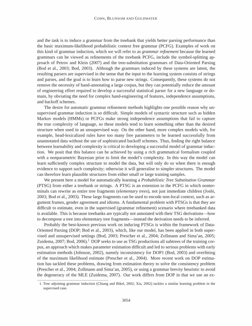
and the task is to induce a grammar from the treebank that yields better parsingperformance thanthe basic maximum-likelihood probabilistic context free grammar (PCFG). Examples of work onthis kind of grammar induction, which we will refer to asgrammar refinementbecause the learnedgrammars can be viewed as refinements of the treebank PCFG, include the symbol-splitting ap-proach of Petrov and Klein (2007) and the tree-substitution grammars of Data-Oriented Parsing(Bod et al., 2003; Bod, 2003). Although the grammars induced by these systems are latent, theresulting parsers are supervised in the sense that the input to the learningsystem consists of stringsand parses, and the goal is to learn how to parse new strings. Consequently, these systems do notremove the necessity of hand-annotating a large corpus, but they can potentially reduce the amountof engineering effort required to develop a successful statistical parser for a new language or do-main, by obviating the need for complex hand-engineering of features, independence assumptions,and backoff schemes.
The desire for automatic grammar refinement methods highlights one possible reason why un-supervised grammar induction is so difficult. Simple models of syntactic structuresuch as hiddenMarkov models (HMMs) or PCFGs make strong independence assumptions that fail to capturethe true complexity of language, so these models tend to learn something other than the desiredstructure when used in an unsupervised way. On the other hand, more complex models with, forexample, head-lexicalized rules have too many free parameters to be learned successfully fromunannotated data without the use of sophisticated backoff schemes. Thus, finding the right balancebetween learnability and complexity is critical to developing a successful model of grammar induc-tion. We posit that this balance can be achieved by using a rich grammatical formalism coupledwith a nonparametric Bayesian prior to limit the model’s complexity. In this way the model canlearn sufficiently complex structure to model the data, but will only do so whenthere is enoughevidence to support such complexity; otherwise it will generalise to simpler structures. The modelcan therefore learn plausible structures from either small or large trainingsamples.
We present here a model for automatically learning aProbabilistic Tree Substitution Grammar(PTSG) from either a treebank or strings. A PTSG is an extension to the PCFG in which nonter-minals can rewrite as entire tree fragments (elementary trees), not just immediate children (Joshi,2003; Bod et al., 2003). These large fragments can be used to encode non-local context, such as ar-gument frames, gender agreement and idioms. A fundamental problem with PTSGs is that they aredifficult to estimate, even in the supervised (grammar refinement) scenario where treebanked datais available. This is because treebanks are typically not annotated with their TSG derivations—howto decompose a tree into elementary tree fragments—instead the derivation needs to be inferred.
Probably the best-known previous work on inducing PTSGs is within the framework of Data-Oriented Parsing (DOP; Bod et al., 2003), which, like our model, has beenapplied in both super-vised and unsupervised settings (Bod, 2003; Prescher et al., 2004; Zollmann and Sima’an, 2005;Zuidema, 2007; Bod, 2006).1 DOP seeks to use as TSG productions all subtrees of the training cor-pus, an approach which makes parameter estimation difficult and led to serious problems with earlyestimation methods (Johnson, 2002), namely inconsistency for DOP1 (Bod,2003) and overfittingof the maximum likelihood estimate (Prescher et al., 2004). More recent workon DOP estima-tion has tackled these problems, drawing from estimation theory to solve the consistency problem(Prescher et al., 2004; Zollmann and Sima’an, 2005), or using a grammar brevity heuristic to avoidthe degeneracy of the MLE (Zuidema, 2007). Our work differs from DOP in that we use an ex-
1. Tree adjoining grammar induction (Chiang and Bikel, 2002; Xia, 2002)tackles a similar learning problem in thesupervised case.
3054

INDUCING TREE SUBSTITUTION GRAMMARS
plicit generative model of TSG and a Bayesian prior for regularisation. The prior is nonparametric,which allows the model to learn a grammar of the appropriate complexity for the size of the train-ing data. A further difference is that instead of seeking to use all subtrees from the training datain the induced TSG, our prior explicitly biases against such behaviour, such that the model learnsa relatively compact grammar.2 A final minor difference is that, because our model is generative,it assigns non-zero probability to all possible subtrees, even those that were not observed in thetraining data. In practice, unobserved subtrees will have very small probabilities.
We apply our model to the two grammar induction problems discussed above:
• Inducing a TSG from a treebank. This regime is analogous to the case of supervised DOP,where we induce a PTSG from a corpus of parsed sentences, and usethis PTSG to parsenew sentences. We present results using two different inference methods, training on eithera subset of WSJ or on the full treebank. We report performance of 84.7% when training onthe full treebank, far better than the 64.2% for a PCFG parser. These gains in accuracy areobtained with a grammar that is somewhat larger than the PCFG grammar, but still muchsmaller than the DOP all-subtrees grammar.
• Inducing a TSG from strings. As in other recent unsupervised parsing work, we adopta dependency grammar (Mel′cuk, 1988) framework for the unsupervised regime. We usethe split-head construction (Eisner, 2000; Johnson, 2007) to map between dependency andphrase-structure grammars, and apply our model to strings of POS tags. We report perfor-mance of 65.9% on the standard WSJ≤10 data set, which is statistically tied with the best re-ported result on the task and considerably better than the EM baseline whichobtains 46.1%.When evaluated on test data with no restriction on sentence length—a more realistic setting—our approach significantly improves the state-of-the-art.
Our work displays some similarities to previous work on both the grammar refinement andunsupervised grammar induction problems, but also differs in a number of ways. Aside from DOP,which we have already discussed, most approaches to grammar refinement can be viewed as symbol-splitting. That is, they allow each nonterminal to be split into a number of subcategories. Themost notable examples of the symbol-splitting approach include Petrov et al. (2006), who use alikelihood-based splitting and merging algorithm, and Liang et al. (2007) and Finkel et al. (2007),who develop nonparametric Bayesian models. In theory, any PTSG can berecast as a PCFG with asufficiently large number of subcategories (one for each unique subtree), so the grammar space ofour model is a subspace of the symbol-splitting grammars. However, the number of nonterminalsrequired to recreate our PTSG grammars in a PCFG would be exorbitant. Consequently, our modelshould be better able to learn specific lexical patterns, such as full noun phrases and verbs withtheir subcategorisation frames, while theirs are better suited to learning subcategories with largermembership, such as the days of the week or count versus mass nouns. The approaches are largelyorthogonal, and therefore we expect that a PTSG with nonterminal refinement could capture bothtypes of concept in a single model, thereby improving performance over either approach alone.
For the unsupervised grammar induction problem we adopt the Dependency Model with Va-lency (DMV; Klein and Manning, 2004) framework that is currently dominant for grammar induc-tion (Cohen et al., 2009; Cohen and Smith, 2009; Headden III et al., 2009; Cohen et al., 2010;
2. The prior favours compact grammars by assigning the majority of probability mass to few productions, and very little(but non-zero) mass to other productions. In practice we use MarkovChain Monte Carlo sampling for inferencewhich results in sparse counts with structural zeros, thus permitting efficient representation.
3055

COHN, BLUNSOM AND GOLDWATER
Spitkovsky et al., 2010). The first grammar induction models to surpass a trivial baseline concen-trated on the task of inducing unlabelled bracketings for strings and were evaluated against tree-bank bracketing gold standard (Clark, 2001; Klein and Manning, 2002). Subsequently the DMVmodel has proved more attractive to researchers, partly because it defined a well founded generativestochastic grammar, and partly due to the popularity of dependency trees in many natural languageprocessing (NLP) tasks. Recent work on improving the original DMV model has focused on threeavenues: smoothing the head-child distributions (Cohen et al., 2009; Cohen and Smith, 2009; Head-den III et al., 2009), initialisation (Headden III et al., 2009; Spitkovsky et al., 2010), and extendingthe conditioning distributions (Headden III et al., 2009). Our work falls intothe final category: byextending the DMV CFG model to a TSG we increase the conditioning context ofhead-child deci-sions within the model, allowing the grammar to directly represent groups of linked dependencies.
Adaptor Grammars (Johnson et al., 2007b) are another recent nonparametric Bayesian modelfor learning hierarchical structure from strings. They instantiate a more restricted class of tree-substitution grammar in which each subtree expands completely, with only terminalsymbols asleaves. Since our model permits nonterminals as subtree leaves, it is more general than AdaptorGrammars. Adaptor Grammars have been applied successfully to induce labeled bracketings fromstrings in the domains of morphology and word segmentation (Johnson, 2008a,b; Johnson and Gold-water, 2009) and very recently for dependency grammar induction (Cohen et al., 2010). The latterwork also introduced a variational inference algorithm for Adaptor Grammar inference; we use asampling method here.
The most similar work to that presented here is our own previous work (Cohn et al., 2009; Cohnand Blunsom, 2010), in which we introduced a version of the model described here, along with twoother papers that independently introduced similar models (Post and Gildea,2009; O’Donnell et al.,2009). Cohn et al. (2009) and Post and Gildea (2009) both present models based on a Dirichletprocess prior and provide results only for the problem of grammar refinement, whereas in thisarticle we develop a newer version of our model using a Pitman-Yor process prior, and also showhow it can be used for unsupervised learning. These extensions are also reported in our recentwork on dependency grammar induction (Blunsom and Cohn, 2010), although in this paper wepresent a more thorough exposition of the model and experimental evaluation. O’Donnell et al.(2009) also use a Pitman-Yor process prior (although their model is slightly different from ours) andpresent unsupervised results, but their focus is on cognitive modeling rather than natural languageprocessing, so their results are mostly qualitative and include no evaluation ofparsing performanceon standard corpora.
To sum up, although previous work has included some aspects of what wepresent here, thisarticle contains several novel contributions. Firstly we present a single generative model capableof both supervised and unsupervised learning, to induce tree substitutiongrammars from eithertrees or strings. We demonstrate that in both settings the model outperforms maximum likelihoodbaselines while also achieving results competitive with the best current systems. The second maincontribution is to provide a thorough empirical evaluation in both settings, examining the effect ofvarious conditions including data size, sampling method and parsing algorithm, and providing ananalysis of the structures that were induced.
In the remainder of this article, we briefly review PTSGs in Section 2 before presenting ourmodel, including versions for both constituency and dependency parsing, in Section 3. In Section 4we introduce two different Markov Chain Monte Carlo (MCMC) methods for inference: a localGibbs sampler and a blocked Metropolis-Hastings sampler. The local sampleris much simpler but
3056

INDUCING TREE SUBSTITUTION GRAMMARS
is only applicable in the supervised setting, where the trees are observed,whereas the Metropolis-Hastings sampler can be used in both supervised and unsupervised settings and for parsing. Wediscuss how to use the trained model for parsing in Section 5, presenting three different parsing al-gorithms. Experimental results for supervised parsing are provided in Section 6, where we comparethe different training and parsing methods. Unsupervised dependencygrammar induction experi-ments are described in Section 7, and we conclude in Section 8.
2. Tree-substitution grammars
A Tree Substitution Grammar3 (TSG) is a 4-tuple,G = (T,N,S,R), whereT is a set ofterminalsymbols, N is a set ofnonterminal symbols, S∈ N is the distinguishedroot nonterminalandR is aset of productions (rules). The productions take the form ofelementary trees—tree fragments4 ofheight≥ 1—where each internal node is labelled with a nonterminal and each leaf is labelled witheither a terminal or a nonterminal. Nonterminal leaves are calledfrontier nonterminalsand formthe substitution (recursion) sites in the generative process of creating trees with the grammar. Forexample, in Figure 1b the S→ NP (VP (V hates) NP) production rewrites the S nonterminal as thefragment (S NP (VP (V hates) NP)).5 This production has the two NPs as its frontier nonterminals.
A derivationcreates a tree by starting with the root symbol and rewriting (substituting) it withan elementary tree, then continuing to rewrite frontier nonterminals with elementary trees until thereare no remaining frontier nonterminals. We can represent derivations assequences of elementarytreese, where each elementary tree is substituted for the left-most frontier nonterminal of the treebeing generated. Unlike Context Free Grammars (CFGs) a syntax tree may not uniquely specify thederivation, as illustrated in Figure 1 which shows two derivations using different elementary treesto produce the same tree.
A Probabilistic Tree Substitution Grammar(PTSG), like a PCFG, assigns a probability to eachrule in the grammar, denotedP(e|c) where the elementary treee rewrites nonterminalc. The proba-bility of a derivatione is the product of the probabilities of its component rules. Thus if we assumethat each rewrite is conditionally independent of all others given its root nonterminalc (as in stan-dard TSG models),6 then we have
P(e) = ∏c→e∈e
P(e|c) . (1)
The probability of a tree,t, and string of words,w, are given by
P(t) = ∑e:tree(e)=t
P(e) and
P(w) = ∑t:yield(t)=w
P(t) ,
3. A TSG is aTree Adjoining Grammar(TAG; Joshi, 2003) without the adjunction operator, which allows insertions atinternal nodes in the tree. This operation allows TAGs to describe the set ofmildly context sensitive languages. ATSG in contrast can only describe the set of context free languages.
4. Elementary trees of height 1 correspond to productions in a context free grammar.5. We use bracketed notation to represent tree structures as linear strings. The parenthesis indicate the hierarchical
structure, with the first argument denoting the node label and the followingarguments denoting child trees. Thenonterminals used in our examples denote nouns, verbs, etc., and theirrespective phrasal types, using a simplifiedversion of the Penn treebank tag set (Marcus et al., 1993).
6. Note that this conditional independence does not hold for our model because (as we will see in Section 3) we integrateout the model parameters.
3057

COHN, BLUNSOM AND GOLDWATER
(a)
S
NP
NP
George
VP
V
hates
NP
NP
broccoli
(b)
S
NP VP
V
hates
NP
NP
George
NP
broccoli
(c)
S
NP
George
VP
V
V
hates
NP
broccoli
(d)
S
NP
George
VP
V NP
broccoli
V
hates
Figure 1: Example derivations for the same tree, where arrows indicate substitution sites. Theleft figures (a) and (c) show two different derivations and the right figures (b) and (d) show theelementary trees used in the respective derivation.
respectively, where tree(e) returns the tree for the derivatione and yield(t) returns the string ofterminal symbols at the leaves oft.
Estimating a PTSG requires learning the sufficient statistics forP(e|c) in (1) based on a trainingsample. Estimation has been done in previous work in a variety of ways, for example using heuristicfrequency counts (Bod, 1993), a maximum likelihood estimate (Bod, 2000) and heldout estimation(Prescher et al., 2004). Parsing involves finding the most probable treefor a given string, that is,argmaxt P(t|w). This is typically simplified to finding the most probable derivation, which can bedone efficiently using the CYK algorithm. A number of improved algorithms for parsing have beenreported, most notably a Monte-Carlo approach for finding the maximum probability tree (Bod,1995) and a technique for maximising labelled recall using inside-outside inference in a PCFGreduction grammar (Goodman, 1998).
2.1 Dependency Grammars
Due to the wide availability of annotated treebanks, phrase structure grammars have become a pop-ular formalism for building supervised parsers, and we will follow this tradition by using phrasestructure trees from the Wall Street Journal corpus (Marcus et al., 1993) as the basis for our su-pervised grammar induction experiments (grammar refinement). However, thechoice of formalismfor unsupervised induction is a more nuanced one. The induction of phrase-structure grammars isnotoriously difficult, since these grammars contain two kinds of ambiguity: the constituent structureand the constituent labels. In particular, constituent labels are highly ambiguous: firstly we don’tknowa priori how many there are, and secondly labels that appear high in a tree (e.g., anScategory
3058

INDUCING TREE SUBSTITUTION GRAMMARS
George hates broccoli ROOT
Figure 2: An unlabelled dependency analysis for the example sentenceGeorge hates broccoli. Theartificial ROOT node denotes the head of the sentence.
for a clause) rely on the correct inference of all the latent labels aboveand below them. Much ofthe recent work on unsupervised grammar induction has therefore takena different approach, fo-cusing on inducing dependency grammars (Mel′cuk, 1988). In applying our model to unsupervisedgrammar induction we follow this trend by inducing a dependency grammar. Dependency gram-mars represent the structure of language through directed links betweenwords, which relate words(heads) with their syntactic dependents (arguments). An example dependency tree is shown in Fig-ure 2, where directed arcs denote each word’s arguments (e.g., hates has two arguments, ‘George’and ‘broccoli’). Dependency grammars are less ambiguous than phrase-structure grammars sincethe set of possible constituent labels (heads) is directly observed from the words in the sentence,leaving only the induction challenge of determining the tree structure. Most dependency grammarformalisms also include labels on the links between words, denoting, for example, subject, object,adjunct etc. In this work we focus on inducing unlabelled directed dependency links and assume thatthese links form a projective tree (there are no crossing links, which correspond to discontinuousconstituents). We leave the problem of inducing labeled dependency grammars to further work.
Although we will be inducing dependency parses in our unsupervised experiments, we defineour model in the following section using the formalism of a phrase-structure grammar. As detailedin Section 7, the model can be used for dependency grammar induction by using a specially designedphrase-structure grammar to represent dependency links.
3. Model
In defining our model, we focus on the unsupervised case, where we are given a corpus of text stringsw and wish to learn a tree-substitution grammarG that we can use to infer the parses for our stringsand to parse new data. (We will handle the supervised scenario, where we are given observed treest, in Section 4; we treat it as a special case of the unsupervised model using additional constraintsduring inference.) Rather than inferring a grammar directly, we go throughan intermediate step ofinferring a distribution over the derivations used to producew, that is, a distribution over sequencesof elementary treese that compose to formw as their yield. We will then essentially read thegrammar off the elementary trees, as described in Section 5. Our problem therefore becomes one ofidentifying the posterior distribution ofe givenw, which we can do using Bayes’ Rule,
P(e|w) ∝ P(w|e)P(e) .
Note that any sequence of elementary trees uniquely specifies a corresponding sequence of words:those words that can be read off the leaves of the elementary trees in sequence. Therefore, given asequence of elementary treese, P(w|e) either equals 1 (ifw is consistent withe) or 0 (otherwise).Thus, in our model, all the work is done by the prior distribution over elementary trees,
P(e|w) ∝ P(e)δ(w(e),w) ,
3059

COHN, BLUNSOM AND GOLDWATER
5
5−a9+b
1−a9+b
2−a9+b
1−a9+b
4a9+b
. . .1 2 3 4
Figure 3: An example of the Pitman-Yor Chinese restaurant process withz−10 =(1,2,1,1,3,1,1,4,3). Black dots indicate the number of customers sitting at each table, and thevalue listed below tablek is P(z10 = k|z−10).
whereδ is the Kronecker delta andw(e) = yield(tree(e)) returns the string yield of the tree definedby the derivatione.
Because we have no way to know ahead of time how many elementary trees mightbe neededto account for the data, we use a nonparametric Bayesian prior, specifically the Pitman-Yor process(PYP) (Pitman, 1995; Pitman and Yor, 1997; Ishwaran and James, 2003), which is a generalizationof the more widely known Dirichlet process (Ferguson, 1973). Drawinga sample from a PYP(or DP) yields a probability distributionG with countably infinite support. The PYP has threeparameters: adiscount parameter a, astrength parameter b, and abase distribution PE. Informally,the base distribution determines which items will be in the support ofG (here, we will definePE
as a distribution over elementary trees, so thatG is also a distribution over elementary trees), andthe discount and strength parametersa andb determine the shape ofG. The discount parameteraranges from 0 to 1; whena= 0, the PYP reduces to a Dirichlet process, in which case the strengthparameterb is known as theconcentration parameterand is usually denoted withα. We discuss theroles ofa andb further below.
Assuming an appropriate definition forPE (we give a formal definition below), we can use thePYP to define a distribution over sequences of elementary treese = e1 . . .en as follows:
G|a,b,PE ∼ PYP(a,b,PE)
ei |G ∼ G. (2)
In this formulation,G is an infinite distribution over elementary trees drawn from the PYPprior, and theei are drawniid from G. However, since it is impossible to explicitly represent aninfinite distribution, we integrate over possible values ofG, which induces dependencies betweentheei . Perhaps the easiest way to understand the resulting distribution overe is through a variantof the Chinese restaurant process (CRP; Aldous, 1985; Pitman, 1995)that is often used to explainthe Dirichlet process. Imagine a restaurant with an infinite number of tables,each with an infinitenumber of seats. Customers enter the restaurant one at a time and seat themselves at a table. Ifzi isthe index of the table chosen by theith customer, then the Pitman-Yor Chinese Restaurant Process(PYCRP) defines the distribution
P(zi = k|z−i) =
n−k −ai−1+b 1≤ k≤ K−
K−a+bi−1+b k= K−+1
,
3060
INDUCING TREE SUBSTITUTION GRAMMARS
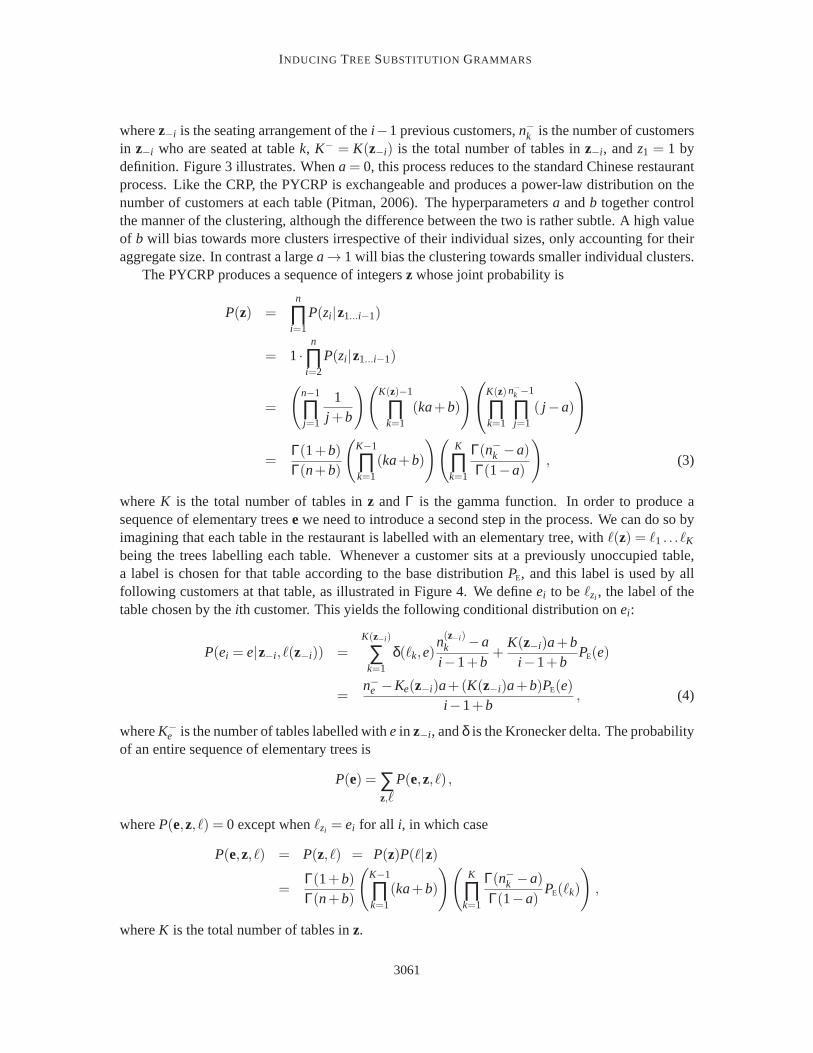
wherez−i is the seating arrangement of thei−1 previous customers,n−k is the number of customersin z−i who are seated at tablek, K− = K(z−i) is the total number of tables inz−i , andz1 = 1 bydefinition. Figure 3 illustrates. Whena= 0, this process reduces to the standard Chinese restaurantprocess. Like the CRP, the PYCRP is exchangeable and produces a power-law distribution on thenumber of customers at each table (Pitman, 2006). The hyperparametersa andb together controlthe manner of the clustering, although the difference between the two is rather subtle. A high valueof b will bias towards more clusters irrespective of their individual sizes, onlyaccounting for theiraggregate size. In contrast a largea→ 1 will bias the clustering towards smaller individual clusters.
The PYCRP produces a sequence of integersz whose joint probability is
P(z) =n
∏i=1
P(zi |z1...i−1)
= 1·n
∏i=2
P(zi |z1...i−1)
=
(n−1
∏j=1
1j +b
)(K(z)−1
∏k=1
(ka+b)
)
K(z)
∏k=1
n−k −1
∏j=1
( j −a)
=Γ(1+b)Γ(n+b)
(K−1
∏k=1
(ka+b)
)(K
∏k=1
Γ(n−k −a)
Γ(1−a)
)
, (3)
whereK is the total number of tables inz and Γ is the gamma function. In order to produce asequence of elementary treese we need to introduce a second step in the process. We can do so byimagining that each table in the restaurant is labelled with an elementary tree, withℓ(z) = ℓ1 . . . ℓK
being the trees labelling each table. Whenever a customer sits at a previouslyunoccupied table,a label is chosen for that table according to the base distributionPE, and this label is used by allfollowing customers at that table, as illustrated in Figure 4. We defineei to beℓzi , the label of thetable chosen by theith customer. This yields the following conditional distribution onei :
P(ei = e|z−i , ℓ(z−i)) =K(z−i)
∑k=1
δ(ℓk,e)n(z−i)
k −a
i−1+b+
K(z−i)a+bi−1+b
PE(e)
=n−e −Ke(z−i)a+(K(z−i)a+b)PE(e)
i−1+b, (4)
whereK−e is the number of tables labelled withe in z−i , andδ is the Kronecker delta. The probability
of an entire sequence of elementary trees is
P(e) = ∑z,ℓ
P(e,z, ℓ) ,
whereP(e,z, ℓ) = 0 except whenℓzi = ei for all i, in which case
P(e,z, ℓ) = P(z, ℓ) = P(z)P(ℓ|z)
=Γ(1+b)Γ(n+b)
(K−1
∏k=1
(ka+b)
)(K
∏k=1
Γ(n−k −a)
Γ(1−a)PE(ℓk)
)
,
whereK is the total number of tables inz.
3061
COHN, BLUNSOM AND GOLDWATER
S
NP VP . . .S
NP VP
VP
V NP
broccoli
PP
IN
in
NP
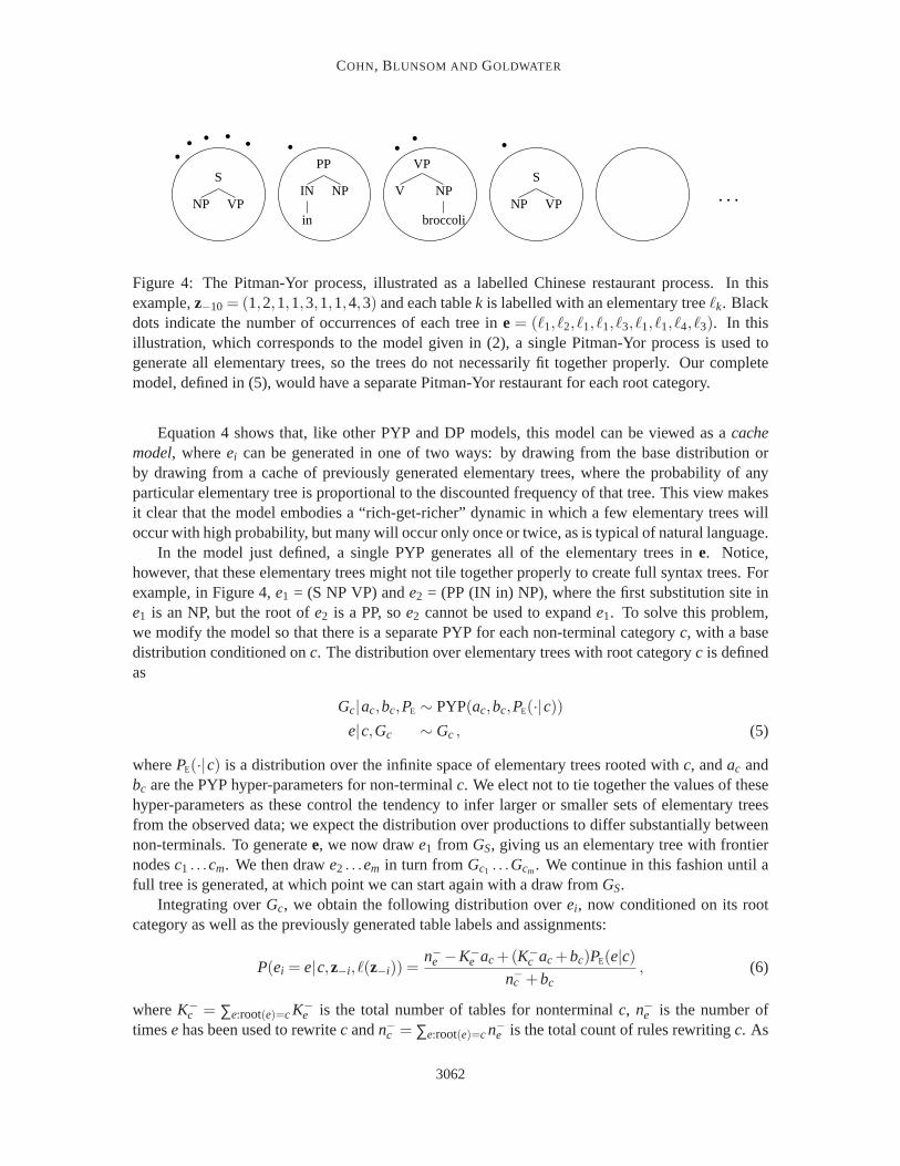
Figure 4: The Pitman-Yor process, illustrated as a labelled Chinese restaurant process. In thisexample,z−10= (1,2,1,1,3,1,1,4,3) and each tablek is labelled with an elementary treeℓk. Blackdots indicate the number of occurrences of each tree ine = (ℓ1, ℓ2, ℓ1, ℓ1, ℓ3, ℓ1, ℓ1, ℓ4, ℓ3). In thisillustration, which corresponds to the model given in (2), a single Pitman-Yorprocess is used togenerate all elementary trees, so the trees do not necessarily fit togetherproperly. Our completemodel, defined in (5), would have a separate Pitman-Yor restaurant for each root category.
Equation 4 shows that, like other PYP and DP models, this model can be viewed as acachemodel, whereei can be generated in one of two ways: by drawing from the base distributionorby drawing from a cache of previously generated elementary trees, where the probability of anyparticular elementary tree is proportional to the discounted frequency of that tree. This view makesit clear that the model embodies a “rich-get-richer” dynamic in which a few elementary trees willoccur with high probability, but many will occur only once or twice, as is typical of natural language.
In the model just defined, a single PYP generates all of the elementary treesin e. Notice,however, that these elementary trees might not tile together properly to create full syntax trees. Forexample, in Figure 4,e1 = (S NP VP) ande2 = (PP (IN in) NP), where the first substitution site ine1 is an NP, but the root ofe2 is a PP, soe2 cannot be used to expande1. To solve this problem,we modify the model so that there is a separate PYP for each non-terminal categoryc, with a basedistribution conditioned onc. The distribution over elementary trees with root categoryc is definedas
Gc|ac,bc,PE ∼ PYP(ac,bc,PE(·|c))
e|c,Gc ∼ Gc , (5)
wherePE(·|c) is a distribution over the infinite space of elementary trees rooted withc, andac andbc are the PYP hyper-parameters for non-terminalc. We elect not to tie together the values of thesehyper-parameters as these control the tendency to infer larger or smallersets of elementary treesfrom the observed data; we expect the distribution over productions to differ substantially betweennon-terminals. To generatee, we now drawe1 from GS, giving us an elementary tree with frontiernodesc1 . . .cm. We then drawe2 . . .em in turn fromGc1 . . .Gcm. We continue in this fashion until afull tree is generated, at which point we can start again with a draw fromGS.
Integrating overGc, we obtain the following distribution overei , now conditioned on its rootcategory as well as the previously generated table labels and assignments:
P(ei = e|c,z−i , ℓ(z−i)) =n−e −K−
e ac+(K−c ac+bc)PE(e|c)
n−c +bc, (6)
whereK−c = ∑e:root(e)=cK−
e is the total number of tables for nonterminalc, n−e is the number oftimesehas been used to rewritec andn−c = ∑e:root(e)=cn−e is the total count of rules rewritingc. As
3062
INDUCING TREE SUBSTITUTION GRAMMARS
before, the− superscript denotes that the counts are calculated over the previous elementary trees,e−i , and their seating arrangements,z−i .
Finally, we turn to the definition of the base distribution over elementary trees,PE. Recall thatin an elementary tree, each internal node is labelled with a non-terminal category symbol and eachfrontier (leaf) node is labelled with either a non-terminal or a terminal symbol. Given a probabilisticcontext-free grammarR, we assume that elementary trees are generated (conditioned on the rootnon-terminalc) using the following generative process. First, choose a PCFG production c → αfor expandingc according to the distribution given byR. Next, for each non-terminal inα decidewhether to stop expanding (creating a non-terminal frontier node, also known as a substitution site)or to continue expanding. If the choice is to continue expanding, a new PCFG production is chosento expand the child, and the process continues recursively. The generative process completes whenthe frontier is composed entirely of substitution sites and terminal symbols.
Assuming a fixed distributionPC over the rules inR, this generative process leads to the follow-ing distribution over elementary trees:
PE(e|c) = ∏i∈I(e)
(1−sci ) ∏f∈F(e)
scf ∏c′→α∈e
PC(α|c′) , (7)
whereI(e) are the set of internal nodes ine excluding the root,F(e) are the set of frontier non-terminal nodes,ci is the non-terminal symbol for nodei andsc is the probability of stopping ex-panding a node labelledc. We treatsc as a parameter which is estimated during training, as de-scribed in Section 4.3. In the supervised case it is reasonable to assume that PC is fixed; we simplyuse the maximum-likelihood PCFG distribution estimated from the training corpus (i.e.,PC(α|c′) issimply the relative frequency of the rulec′ → α). In the unsupervised case, we will inferPC; thisrequires extending the model to assume thatPC is itself drawn from a PYP prior with a uniform basedistribution. We describe this extension below, along with its associated changes to equation 14.
The net effect of our base distribution is to bias the model towards simple rules with a smallnumber of internal nodes. The geometric increase in cost associated with the stopping decisionsdiscourages the model from using larger rules; for these rules to be included they must occur veryfrequently in the corpus. Similarly, rules which use high-probability (frequent) CFG productionsare favoured. It is unclear if these biases are ideal: we anticipate that other, more sophisticateddistributions would improve the model’s performance.
In the unsupervised setting we no longer have a training set of annotated trees and therefore donot have a PCFG readily available to use as the base distribution in Equation 7.For this reason weextend the previous model to a two level hierarchy of PYPs. As before, the topmost level is definedover the elementary tree fragments (Gc) with the base distribution (PE) assigning probability to theinfinite space of possible fragments. The model differs from the supervised one by definingPC
in (7) using a PYP prior over CFG rules. Accordingly the model can now infer a two level hierarchyconsisting of a PCFG embedded within a TSG, compared to the supervised parsing model whichonly learnt the TSG level with a fixed PCFG. Formally, each CFG production isdrawn from7
Hc|a′c,b
′c ∼ PYP(a′c,b
′c,Uniform(·|c))
α|c,Hc ∼ Hc , (8)
7. As we are using a finite base distribution over CFG productions, we coulduse a Dirichlet instead of the PYP presentedin (8). However we elect to use a PYP because it is more general, havingadditional expressive power from itsdiscounting behaviour.
3063

COHN, BLUNSOM AND GOLDWATER
wherea′c and b′c are the PYP hyper-parameters and Uniform(·|c) is a uniform distribution overthe space of rewrites for non-terminalc.8 As before, we integrate out the model parameters,Hc.Consequently draws fromPC are no longeriid but instead are tied in the prior, and the probabilityof the sequence of component CFG productions{c′ → α ∈ e} now follows a Pitman-Yor ChineseRestaurant Process.
The CFG level and TSG level PYCRPs are connected as follows: every timean elementary treeis assigned to a new table in the TSG level, each of its component CFG rules aredrawn from theCFG level prior. Note that, just as elementary trees are divided into separate restaurants at the TSGlevel based on their root categories, CFG rules are divided into separate restaurants at the CFG levelbased on their left-hand sides. Formally, the probability ofr j , the j th CFG rule in the sequence, isgiven by
PC(r j = r|c j = c,z′− j , ℓ′− j) =
n′−r −K′−r a′c+(K′−
c a′c+b′c)1
|Rc|
K′−c +b′c
, (9)
wherec j is the left-hand side ofr j ; z′− j andℓ′− j are the table assignments and table labels in theCFG-level restaurants (we use prime symbols to indicate variables pertainingto the CFG level);n′−r is the number of times ruler is used in any table label in a TSG restaurant (equivalently, thenumber of customers at tables labelledr in the CFG restaurants);K′−
r andK′−c = ∑r:root(r)=cK′−
rare the CFG-level table counts forr and all rules rewritingc, respectively; andRc is the set ofCFG productions which can rewritec. This formulation reflects that we now have multiple tiedrestaurants, and each time an elementary tree opens a new table in a top-levelrestaurant all itsrules are considered to have entered their own respectivePC restaurants (according to their rootc).Accordingly the CFG-level customer count,n′−r , is the number of occurrences ofr in the elementarytrees that label the tables in the TSG restaurants (excludingr j ). Thus, in the unsupervised case, theproduct of rule probabilities (the final factor) in Equation (7) is computed by multiplying togetherthe conditional probability of each rule (9) given the previous ones.
4. Training
We present two alternative algorithms for training our model, both based on Markov chain MonteCarlo techniques, which produce samples from the posterior distribution ofthe model by iterativelyresampling the values of the hidden variables (tree nodes). The first algorithm is a local sampler,which operates by making a local update to a single tree node in each sampling step. The secondalgorithm is ablockedsampler, which makes much larger moves by sampling analyses for full sen-tences, which should improve the mixing over the local sampler. Importantly the blocked sampler ismore general, being directly applicable to both supervised and unsupervised settings (and for pars-ing test sentences, which is equivalent to an unsupervised setting) while the local sampler is onlyapplicable for supervised learning, where the trees are observed. Wenow present the two samplingmethods in further detail.
8. In our experiments on unsupervised dependency parsing the space of rewrites varied depending onc, and can be aslarge as the set of part-of-speech tags. See Section 7 for details.
3064

INDUCING TREE SUBSTITUTION GRAMMARS
(a)
S
NP
NP
George
VP
V
hates
NP
NP
broccoli
(b)
S
NP,1
George
VP,0
V,0
hates
NP,1
broccoli
Figure 5: Gibbs sampler state (b) corresponding to the example derivation (a) (reproduced fromFigure 1a). Each node is labelled with its substitution variable.
4.1 Local Sampler
Thelocal sampler is designed specifically for the supervised scenario, and samplesa TSG derivationfor each tree by sampling local updates at each tree node. It uses Gibbs sampling (Geman andGeman, 1984), where random variables are repeatedly sampled conditioned on the current values ofall other random variables in the model. The actual algorithm is analogous to the Gibbs sampler usedfor inference in the Bayesian model of word segmentation presented by Goldwater et al. (2006);indeed, the problem of inferring the derivationse from t can be viewed as a segmentation problem,where each full tree must be segmented into one or more elementary trees. Toformulate the localsampler, we associate a binary variablexd ∈ {0,1} with each non-root internal node,d, of eachtree in the training set, indicating whether that node is a substitution point (xd = 1) or not (xd = 0).Each substitution point forms the root of some elementary tree, as well as a frontier nonterminalof an ancestor node’s elementary tree. Conversely, each non-substitution point forms an internalnode inside an elementary tree. Collectively the training trees and substitution variables specify thesequence of elementary treese that is the current state of the sampler. Figure 5 shows an exampletree with its substitution variables and its corresponding TSG derivation.
Our Gibbs sampler works by sampling the value of thexd variables, one at a time, in randomorder. If d is the node associated withxd, the substitution variable under consideration, then thetwo possible values ofxd define two options fore: one in whichd is internal to some elementarytreeeM, and one in whichd is the substitution site connecting two smaller trees,eA andeB. In theexample in Figure 5, when sampling the VP node,eM = (S NP (VP (V hates) NP)),eA = (S NP VP),andeB = (VP (V hates) NP). To sample a value forxd, we compute the probabilities ofeM and(eA,eB), conditioned one−: all other elementary trees in the training set that share at most a root orfrontier nonterminal witheM,eA, or eB. These probabilities are easy to compute because the PYP isexchangeable, meaning that the probability of a set of outcomes does not depend on their ordering.Therefore we can treat the elementary trees under consideration as the last ones to be sampled, andapply Equation (6). We then sample one of the two outcomes (merging or splitting)according to therelative probabilities of these two events. More specifically, the probabilitiesof the two outcomes,
3065

COHN, BLUNSOM AND GOLDWATER
conditioned on the current analyses of the remainder of the corpus, are
P(eM|cM) =n−eM
−K−eM
acM +(K−cM
acM +bcM)PE(eM|cM)
n−cM +bcM
and
P(eA,eB|cA,cB) = ∑zeA
P(eA,zeA|cA)P(eB|eA,zeA,cA,cB)
=n−eA
−K−eA
acA
n−cA +bcA
×n−eB
+δe−K−eB
acB +(K−cB
acB +bcB)PE(eB|cB)
n−cB +δc+bcB
+(K−
cAacA +bcA)PE(eA|cA)
n−cA +bcA
×n−eB
+δe− (K−eB+δe)acB +
((K−
cB+δc)acB +bcB
)PE(eB|cB)
n−cB +δc+bcB
, (10)
wherecy is the root label ofey, the countsn− and K− are derived fromz−M and ℓ(z−M) (thisdependency is omitted from the conditioning context for brevity),δe = δ(eA,eB) is the Kroneckerdelta function which has value one wheneA andeB are identical and zero otherwise, and similarly forδc = δ(cA,cB) which compares their root nonterminalscA andcB. Theδ terms reflect the changesto n− that would occur after observingeA, which forms part of the conditioning context foreB.The two additive terms in (10) correspond to different values ofzeA, the seating assignment foreA.Specifically, the first term accounts for the case whereeA is assigned to an existing table,zeA < K−
eA,
and the second term accounts for the case whereeA is seated at a new table,zeA = K−eA
. The seatingaffects the conditional probability ofeB by potentially increasing the number of tablesK−
eAor K−
cA
(relevant only wheneA = eB or cA = cB).
4.2 Blocked Sampler
The local sampler has the benefit of being extremely simple, however it may suffer from slowconvergence (poor mixing) due to its very local updates. That is, it can get stuck because manylocally improbable decisions are required to escape from a locally optimal solution. Moreover it isonly applicable to the supervised setting: it cannot be used for unsupervised grammar induction orfor parsing test strings. For these reasons we develop theblockedsampler, which updates blocks ofvariables at once, where each block consists of all the the nodes associated with a single sentence.This sampler can make larger moves than the local sampler and is more flexible, in that it canperform inference with both string (unsupervised) or tree (supervised) input.9
The blocked sampler updates the analysis for each sentence given the analyses for all othersentences in the training set. We base our approach on the algorithm developed by Johnson et al.(2007a) for sampling parse trees using a finite Bayesian PCFG model with Dirichlet priors over themultinomial rule probabilities. As in our model, they integrate out the parameters (intheir case,the PCFG rule probabilities), leading to a similar caching effect due to interdependences betweenthe latent variables (PCFG rules in the parse). Thus, standard dynamic programming algorithmscannot be used to sample directly from the desired posterior,p(t|w, t−), that is, the distributionof parse trees for the current sentence given the words in the corpusand the trees for all othersentences. To solve this problem, Johnson et al. (2007a) developed a Metropolis-Hastings (MH)
9. A recently-proposed alternative approach is to performtype-levelupdates, which samples updates to many similartree fragments at once (Liang et al., 2010). This was shown to converge faster than the local Gibbs sampler.
3066

INDUCING TREE SUBSTITUTION GRAMMARS
sampler. The MH algorithm is an MCMC technique which allows for samples to be drawn froma probability distribution,π(s), by first drawing samples from aproposal distribution, Q(s′|s), andthen correcting these to the true distribution using an acceptance/rejection step. Given a states,we sample a next states′ ∼ Q(·|s) from the proposal distribution; this new state is accepted withprobability
A(s,s′) = min
{π(s′)Q(s|s′)π(s)Q(s′|s)
,1
}
and is rejected otherwise, in which cases is retained as the current state. The Markov chain definedby this process is guaranteed to converge on the desired distribution,π(s). Critically, the MHalgorithm enables sampling from distributions from which we cannot sample directly, and moreover,we need not know the normalisation constant forπ(·), since it cancels inA(s,s′).
In Johnson et al.’s (2007a) algorithm for sampling from a Bayesian PCFG, the proposal distri-bution is simplyQ(t ′|t) = P(t ′|θMAP), the posterior distribution over trees given fixed parametersθMAP, whereθMAP is the MAP estimate based on the conditioning data,t−. Note that the proposaldistribution is a close fit to the true posterior, differing only in that under the MAP the productionprobabilities in a derivation areiid, while for the true model the probabilities are tied by the prior(giving rise to the caching effect). The benefit of using the MAP is that its independences mean thatinference can be solved using dynamic programming, namely the inside algorithm (Lari and Young,1990). Given the inside chart, which stores the aggregate probability of all subtrees for each wordspan and rooted with a given nonterminal label, samples can be drawn usinga simple top-downrecursion (Johnson et al., 2007a).
Our model is similar to Johnson et al.’s, as we also use a Bayesian prior in a model of grammarinduction and consequently face similar problems with directly sampling due to the caching effectsof the prior. For this reason, we use the MH algorithm in a similar manner, except in our case wedraw samples of derivations of elementary trees and their seating assignments, p(zi , ℓi |w,z−i , ℓ−i),and use a MAP estimate over(z−i , ℓi−) as our proposal distribution.10 However, we have an addedcomplication: the MAP cannot be estimated directly. This is a consequence of the base distributionhaving infinite support, which means the MAP has an infinite rule set. For finite TSG models, suchas those used in DOP, constructing a CFG equivalent grammar is straightforward (if unwieldy).This can be done by creating a rule for each elementary tree which rewritesits root nontermi-nal as its frontier. For example under this techniqueS→ NP (VP (V hates) NPwould be mappedto S→ NP hates NP.11 However, since our model has infinite support over productions, it cannotbe mapped in the same way. For example, if our base distribution licences the CFG productionNP→ NP PPthen our TSG grammar will contain the infinite set of elementary treesNP→ NP PP,NP→ (NP NP PP) PP, NP→ (NP (NP NP PP) PP) PP, . . . , each with decreasing but non-zero proba-bility. These would all need to be mapped to CFG rules in order to perform inference under thegrammar, which is clearly impossible.
Thankfully it is possible to transform the infinite MAP-TSG into a finite CFG, usinga methodinspired by Goodman (2003), who developed a grammar transform for efficient parsing with an
10. Calculating the proposal and acceptance probabilities requires sampling not just the elementary trees, but also theirtable assignments (for both levels in the hierarchical model). We elected to simplify the implementation by separatelysampling the elementary trees and their table assignments.
11. Alternatively, interspersing a special nonterminal, for example, S→ {S-NP-{VP-{V-hates}-NP} → NP hates NP,encodes the full structure of the elementary tree, thereby allowing the mapping to be reversed. We use a similartechnique to encode non-zero count rules in our grammar transformation, described below.
3067

COHN, BLUNSOM AND GOLDWATER
all-subtrees DOP grammar. In the transformed grammar inside inference is tractable, allowing us todraw proposal samples efficiently and thus construct a Metropolis-Hastings sampler. The resultantgrammar allows for efficient inference, both in unsupervised and supervised training and in parsing(see Section 5).
We represent the MAP using the grammar transformation in Table 1, which separates the countand base distribution terms in Equation 6 into two separate CFGs, denoted A andB. We reproduceEquation 6 below along with its decomposition:
P(ei = e|c,z−i , ℓ(z−i)) =n−e −K−
e ac+(K−c ac+bc)PE(e|c)
n−c +bc
=n−e −K−
e ac
n−c +bc︸ ︷︷ ︸
count
+K−
c ac+bc
n−c +bcPE(e|c)
︸ ︷︷ ︸
base
. (11)
Grammar A has productions for every elementary treee with n−e ≥ 1, which are assigned as theirprobability the count term in Equation 11.12 The function sig(e) returns a string signature for el-ementary trees, for which we use a form of bracketed notation. To signifythe difference betweenthese nonterminal symbols and trees, we use curly braces and hyphens inplace of round parenthesesand spaces, respectively, for example, the elementary tree (S NP (VP (Vhates) NP)) is denoted bythe nonterminal symbol{S-NP-{VP-{V-hates}-NP}}. Grammar B has productions for every CFGproduction licensed underPE; its productions are denoted using primed (’) nonterminals. The rulec→ c′ bridges from A to B, weighted by the base term in Equation 11 excluding thePE(e|c) factor.The contribution of the base distribution is computed recursively via child productions. The remain-ing rules in grammar B correspond to every CFG production in the underlyingPCFG base distribu-tion, coupled with the binary decision of whether or not nonterminal children should be substitutionsites (frontier nonterminals). This choice affects the rule probability by including ans or 1−s fac-tor, and child substitution sites also function as a bridge back from grammar B toA. There are oftentwo equivalent paths to reach the same chart cell using the same elementary tree—via grammar Ausing observed TSG productions and via grammar B usingPE backoff—which are summed to yieldthe desired net probability. The transform is illustrated in the example in Figures 6 and 7.
Using the transformed grammar we can represent the MAP grammar efficientlyand draw sam-ples of TSG derivations using the inside algorithm. In an unsupervised setting, that is, given ayield string as input, the grammar transform above can be used directly with theinside algorithmfor PCFGs (followed by the reverse transform to map the sampled derivation into TSG elementarytrees). This has an asymptotic time complexity cubic in the length of the input.
For supervised training the trees are observed and thus we must ensurethat the TSG analysismatches the given tree structure. This necessitates constraining the inside algorithm to only considerspans that are present in the given tree and with the given nonterminal. Nonterminals are said tomatch their primed and signed counterparts, for example, VP′ and{VP-{V-hates}-NP} both matchVP. A sample from the constrained inside chart will specify the substitution variables for each nodein the tree: For each noded if it has a non-primed category in the sample then it is a substitution
12. The transform assumes inside inference, where alternate analyses for the same span of words with the same non-terminal are summed together. In Viterbi inference the summation is replaced by maximisation, and therefore weneed different expansion probabilities. This requires changing the weight for c→ sig(e) to P(ei = e|c,z−i , ℓ(z−i)) inTable 1.
3068

INDUCING TREE SUBSTITUTION GRAMMARS
Gra
mm
arA For every ET,e, rewritingc with non-zero count:
c→ sig(e) n−e −K−e ac
n−c +bc
For every internal nodeei in ewith childrenei,1, . . . ,ei,n
sig(ei)→ sig(ei,1) . . .sig(ei,n) 1A→
B For every nonterminal,c:
c→ c′ K−c ac+bc
n−c +bc
Gra
mm
arB
For every pre-terminal CFG production,c→ t:c′ → t PC(c→ t)
For every unary CFG production,c→ a:c′ → a PC(c→ a)sa
c′ → a′ PC(c→ a)(1−sa)
For every binary CFG production,c→ ab:c′ → ab PC(c→ ab)sasb
c′ → ab′ PC(c→ ab)sa(1−sb)
c′ → a′b PC(c→ ab)(1−sa)sb
c′ → a′b′ PC(c→ ab)(1−sa)(1−sb)
Table 1: Grammar transformation rules to map an infinite MAP TSG into an equivalent CFG,separated into three groups for grammar A (top), the bridge between A→ B (middle) and grammarB (bottom). Production probabilities are shown to the right of each rule. Thesig(e) function createsa unique string signature for an ETe (where the signature of a frontier node is itself) andsc is theprobability ofc being a substitution variable, thus stopping thePE recursion.
S→ {NP-{VP-{V-hates}-NP}} n−e −K−e aS
n−S+bS
{NP-{VP-{V-hates}-NP}} → NP{VP-{V-hates}-NP} 1{VP-{V-hates}-NP} → {V-hates} NP 1{V-hates} → hates 1
S→ S’K−
S aS+bS
n−S+bS
S’ → NP VP’ PC(S→ NP VP)sNP(1−sVP)VP’ → V’ NP PC(VP→ V NP)(1−sV)sNP
V’ → hates PC(V → hates)
Figure 6: Example showing the transformed grammar rules for the single elementary treee =(S NP (VP (V hates) NP)) and the scores for each rule. Only the rules which correspond toeand itssubstitution sites are displayed. Taking the product of the rule scores above the dashed line yieldsthecountterm in (11), and the product of the scores below the line yields thebaseterm. When thetwo analyses are combined and their probabilities summed together, we getP(ei = e|c,z−i , ℓ(z−i)).
3069

COHN, BLUNSOM AND GOLDWATER
S
{S-NP-{VP-{V-hates}-NP}}
NP
George
{VP-{V-hates}-NP}
{V-hates}
hates
NP
broccoli
S
S’
NP
George
VP’
V’
hates
NP
broccoli
Figure 7: Example trees under the grammar transform, which both encode thesame TSG deriva-tion from Figure 1a. The left tree encodes that theS→ NP (VP (V hates) NPelementary tree wasdrawn from the cache, while for the right tree this same elementary tree was drawn from the basedistribution (the count and base terms in (11), respectively).
site,xd = 1, otherwise it is an internal node,xd = 0. For example, both trees in Figure 7 encode thatboth NP nodes are substitution sites and that the VP and V nodes are not substitution sites (the sameconfiguration as Figure 5).
The time complexity of the constrained inside algorithm is linear in the size of the treeand thelength of the sentence. The local sampler also has the same time complexity, however it is not im-mediately clear which technique will be faster in practise. It is likely that the blocked sampler willhave a slower runtime due to its more complicated implementation, particularly in transformingthe grammar and inside inference. Although the two samplers have equivalent asymptotic com-plexity, the constant factors may differ greatly. In Section 6 we compare thetwo training methodsempirically to determine which converges more quickly.
4.3 Sampling Hyperparameters
In the previous discussion we assumed that we are given the model hyperparameters,(a,b,s). Whileit might be possible to specify their values manually or fit them using a development set, bothapproaches are made difficult by the high dimensional parameter space. Instead we treat the hyper-parameters as random variables in our model, by placing vague priors over them and infer theirvalues during training. This is an elegant way to specify their values, although it does limit ourability to tune the model to optimise a performance metric on held-out data.
For the PYP discount parametersa, we employ independent Beta priors,ac ∼ Beta(1,1). Theprior is uniform, encoding that we have no strong prior knowledge of what the value of eachac
should be. The conditional probability ofac given the current derivationsz, ℓ is
P(ac|z, ℓ) ∝P(z, ℓ|ac)×Beta(ac|1,1) .
We cannot calculate the normaliser for this probability, howeverP(z, ℓ|ac) can be calculated usingEquation 3 and thusP(ac|z, ℓ) can be calculated up to a constant. We use the range doubling slicesampling technique of Neal (2003) to draw a new sample ofa′c from its conditional distribution.13
We treat the concentration parameters,b, as being generated by independent gamma priors,bc ∼ Gamma(1,1). We use the same slice-sampling method forac to sample from the conditional
13. We used the slice sampler included in Mark Johnson’s Adaptor Grammar implementation, available athttp://web.science.mq.edu.au/ ˜ mjohnson/Software.htm .
3070

INDUCING TREE SUBSTITUTION GRAMMARS
overbc,
P(bc|z, ℓ) ∝P(z, ℓ|bc)×Gamma(bc|1,1) .
This prior is not vague, that is, the probability density function decays exponentially for highervalues ofbc, which serves to limits the influence of thePC prior. In our experimentation we foundthat this bias had little effect on the generalisation accuracy of the supervised and unsupervisedmodels, compared to a much vaguer Gamma prior with the same mean.
We use a vague Beta prior for the stopping probabilities inPE, sc ∼ Beta(1,1). The Beta dis-tribution is conjugate to the binomial, and therefore the posterior is also a Beta distribution fromwhich we can sample directly,
sc ∼ Beta
(
1+∑e
Ke(z) ∑n∈F(e)
δ(n,c), 1+∑e
Ke(z) ∑n∈I(e)
δ(n,c)
)
,
wheree ranges over all non-zero count elementary trees,F(e) are the nonterminal frontier nodesin e, I(e) are the non-root internal nodes and theδ terms count the number of nodes ine withnonterminalc. In other words, the first Beta argument is the number of tables in which a node withnonterminalc is a stopping node in thePE expansion and the second argument is the number oftables in whichc has been expanded (a non-stopping node).
All the hyper-parameters are resampled after every full sampling iteration over the training trees,except in the experiments in Section 7 where they are sampled every 10th iteration.
5. Parsing
We now turn to the problem of using the model to parse novel sentences. This requires finding themaximiser of
p(t|ω,w) =∫ ∫ ∫ ∫
p(t|ω,z, ℓ,a,b,s) p(z, ℓ,a,b,s|w) dz dℓ da db ds , (12)
whereω is the sequence of words being parsed,t is the resulting tree,w are the training sentences,z andℓ represent their parses, elementary tree representation and table assignments and(a,b,s) arethe model’s hyper-parameters. For the supervised case we use the training trees,t, in place ofw inEquation 12.
Unfortunately solving for the maximising parse tree in Equation 12 is intractable.However, itcan be approximated using Monte Carlo techniques. Given a sample of(z, ℓ,a,b,s) we can reasonover the space of possible TSG derivations,e, for sentencew using the same Metropolis-Hastingssampler presented in Section 4.2 for blocked inference in the unsupervised setting.14 This gives usa set of samples from the posteriorp(e|w,z, ℓ,a,b,s). We then use a Monte Carlo integral to obtaina marginal distribution over trees (Bod, 2003),
pMPT(t) =M
∑m=1
δ(t, tree(em)) , (13)
14. Using many samples in a Monte Carlo integral is a straight-forward extension to our parsing algorithm. We did notobserve a significant improvement in parsing accuracy when using a multiple samples compared to a single sample,and therefore just present results for a single sample. However, using multiple models has been shown to improvethe performance of other parsing models (Petrov, 2010).
3071

COHN, BLUNSOM AND GOLDWATER
where{em}Mm=1 are our sample of derivations forw. It is then straightforward to find the best parse,
t∗ = argmax ˆp(t), which is simply the most frequent tree in the sample.In addition to solving from the maximum probability tree (MPT) using Equation 13,we also
present results for a number of alternative objectives. To test whetherthe derivational ambiguity isimportant, we also compute the maximum probability derivation (MPD),
pMPD(e) =M
∑m=1
δ(e,em) ,
using a Monte-Carlo integral, from which we recover the tree,t∗ = tree(argmaxe pMPD(e)). We alsocompare using the Viterbi algorithm directly with the MAP grammar,t∗ = tree(argmaxe PMAP(e|w)),which constitutes an approximation to the true model in which we can search exactly. This contrastswith the MPD which performs approximate search under the true model. We compare the differentmethods empirically in Section 6.
The MPD and MPT parsing algorithms require the computation of Monte-Carlo integrals overthe large space of possible derivations or trees. Consequently, unlessthe distribution is extremelypeaked the chance of sampling many identical structures is small, vanishingly sofor long sentences(the space of trees grows exponentially with the sentence length). In otherwords, the samplingvariance can be high which could negatively affect parsing performance. For this reason we presentan alternative parsing method which compiles more local statistics for which we can obtain reliableestimates. The technique is based on Goodman’s (2003) algorithm for maximising labelled recall inDOP parsing and subsequent work on parsing in state-splitting CFGs (Petrov and Klein, 2007). Thefirst step is to acquire marginal distributions over the CFG productions within each sampled tree.Specifically, we collect counts for events of the form(c→ α, i, j,k), wherec→ α is a CFG produc-tion spanning words[i, j) andk is the split point between child constituents for binary productions,i < k< j (k= 0 for unary productions). These counts are then marginalised by the number of treessampled. Finally the Viterbi algorithm is used to find the tree with the maximum cumulative proba-bility under these marginals, which we call the maximum expected rule (MER) parse. Note that thisis a type of minimum Bayes risk decoding and was first presented in Petrov and Klein (2007) as theMAX-RULE-SUM method (using exact marginals, not Monte-Carlo estimates as is done here).
6. Supervised Parsing Experiments
In this section we present an empirical evaluation of the model on the task of supervised parsing.In this setting the model learns a segmentation of a training treebank, which defines a TSG. Wepresent parsing results using the learned grammar, comparing the effectsof the sampling strategy,initialisation conditions, parsing algorithm and the size of the training set. The unsupervised modelis described in the following section, Section 7.
We trained the model on the WSJ part of Penn. treebank (Marcus et al., 1993) using the standarddata splits, as shown in Table 2. As our model is parameter free (thea,b,s parameters are learntin training), we do not use the development set for parameter tuning. We expect that fitting thehyperparameters to maximise performance on the development set would leadto a small increasein generalisation performance, but at a significant cost in runtime. We adopt Petrov et al.’s (2006)method for data preprocessing: right-binarizing the trees to limit the branching factor and replacingtokens with count≤ 1 in the training sample with one of roughly 50 generic unknown word markerswhich convey the token’s lexical features and position. The predicted trees are evaluated using
3072

INDUCING TREE SUBSTITUTION GRAMMARS
Partition sections sentences tokens types types (unk)training 2–21 33180 790237 40174 21387
development 22 1700 40117 6840 5473testing 23 2416 56684 8421 6659
small training 2 1989 48134 8503 3728
Table 2: Corpus statistics for supervised parsing experiments using the Penn treebank, reporting foreach partition its WSJ section/s, the number of sentences, word tokens and unique word types. Thefinal column shows the number of word types after unknown word processing using the full trainingset, which replaces rare words with placeholder tokens. The number of types after preprocessing inthe development and testing sets is roughly halved when using the the small training set.
EVALB15 and we report the F1 score over labelled constituents and exact match accuracy over allsentences in the testing sets.
In our experiments, we initialised the sampler by setting all substitution variables to0, thustreating every full tree in the training set as an elementary tree. Unless otherwise specified, theblocked sampler was used for training. We later evaluated the effect of different starting conditionson the quality of the configurations found by the sampler and on parsing accuracy. The sampler wastrained for 5000 iterations and we use the final sample ofz, ℓ,a,b,s for parsing. We ran all fourdifferent parsing algorithms and compare their results on the testing sets. For the parsing methodsthat require a Monte Carlo integral (MPD, MPT and MER), we sampled 1000derivations from theMAP approximation grammar which were then input to the Metropolis-Hastings acceptance stepbefore compiling the relevant statistics. The Metropolis-Hastings acceptance rate was around 99%for both training and parsing. Each experiment was replicated five times andthe results averaged.
6.1 Small Data Sample
For our first treebank experiments we train on a small data sample by using only section 2 of thetreebank (see Table 2 for corpus statistics.) Bayesian methods tend to do well with small datasamples, while for larger samples the benefits diminish relative to point estimates.For this reasonwe present a series of exploratory experiments on the small data set before moving to the fulltreebank.
In our experiments we aim to answer the following questions: Firstly, in terms ofparsing ac-curacy, does the Bayesian TSG model outperform a PCFG baseline, andhow does it compare toexisting high-quality parsers? We will also measure the effect of the parsing algorithm: Viterbi,MPD, MPT and MER. Secondly, which of the local and blocked sampling techniques is more effi-cient at mixing, and which is faster per iteration? Finally, what kind of structures does the modellearn and do they match our expectations? The hyper-parameter values are also of interest, partic-ularly to evaluate whether the increased generality of the PYP is justified overthe DP. Our initialexperiments aim to answer these questions on the small data set, after which wetake the best modeland apply it to the full set.
Table 3 presents the prediction results on the development set. The baselineis a maximum like-lihood PCFG. The TSG models significantly outperform the baseline. This confirms our hypothesisthat CFGs are not sufficiently powerful to model syntax, and that the increased context afforded to
15. Seehttp://nlp.cs.nyu.edu/evalb/ .
3073

COHN, BLUNSOM AND GOLDWATER
Model Viterbi MPD MPP MER # rules
PCFG 60.20 60.20 60.20 - 3500TSG PYP 74.90 76.68 77.17 78.59 25746TSG DP 74.70 75.86 76.24 77.91 25339Berkeley parser (τ = 2) 71.93 71.93 - 74.32 16168Berkeley parser (τ = 5) 75.33 75.33 - 77.93 39758
Table 3: Development results for models trained on section 2 of the Penn treebank, showing labelledconstituent F1 and the grammar size. For the TSG models the grammar size reported is the numberof CFG productions in the transformed MAP PCFG approximation. Unknown word models areapplied to words occurring less than two times (TSG models and Berkeleyτ = 2) or less than fivetimes (Berkeleyτ = 5).
the TSG can make a large difference. Surprisingly, the MPP technique is only slightly better thanthe MPD approach, suggesting that derivational ambiguity is not as much ofa problem as previouslythought (Bod, 2003). Also surprising is the fact that exact Viterbi parsing under the MAP approx-imation is much worse than the MPD method which uses an approximate search technique underthe true model. The MER technique is a clear winner, however, with considerably better F1 scoresthan either MPD or MPP, with a margin of 1–2 points. This method is less affectedby samplingvariance than the other MC algorithms due to its use of smaller tree fragments (CFG productions ateach span).
We also consider the difference between using a Dirichlet process prior(DP) and a Pitman-Yorprocess prior (PYP). This amounts to whether thea hyper-parameters are set to 0 (DP) or are allowedto take on non-zero values (PYP), in which case we sample their values as described in Section 4.3.There is a small but consistent gain of around 0.5 F1 points across the different parsing methodsfrom using the PYP, confirming our expectation that the increased flexibility of the PYP is usefulfor modelling linguistic data. Figure 8a shows the learned values of the PYP hyperparameters aftertraining for each nonterminal category. It is interesting to see that the hyper-parameter values mostlyseparate the open-class categories, which denote constituents carryingsemantic content, from theclosed-class categories, which are largely structural. The open classes (noun-, verb-, adjective- andadverb-phrases: NP, VP, ADJP and ADVP, respectively) tend to have highera andb values (towardsthe top right corner of the graph) and therefore can describe highly diverse sets of productions. Incontrast, most of the closed classes (the root category, quantity phrases, wh-question noun phrasesand sentential phrases: TOP, QP, WHNP and S, respectively) have lowa andb (towards the bottomleft corner of the graph), reflecting that encoding their largely formulaicrewrites does not necessitatediverse distributions.
The s hyper-parameter values are shown in Figure 8b, and are mostly in the mid-range (0.3–0.7). Prepositions (IN), adverbs (RB), determiners (DT) and some tenses of verbs (VBD and VBP)have very lows values, and therefore tend to be lexicalized into elementary trees. This is expectedbehaviour, as these categories select strongly for the words they modifyand some (DT, verbs) mustagree with their arguments in number and tense. Conversely particles (RP),modal verbs (MD) andpossessive particles (PRP$) have highs values, and are therefore rarely lexicalized. This is rea-sonable for MD and PRP$, which tend to be exchangeable for one another without rendering thesentence ungrammatical (e.g., ‘his’ can be substituted for ‘their’ and ‘should’ for ‘can’). However,
3074

INDUCING TREE SUBSTITUTION GRAMMARS
(a) PYP hyper-parameters,a,b
0.2 0.3 0.4 0.5 0.6 0.7 0.8
25
1020
50
a
b
ADJPADVPNPPPQPSSBARSINVTOPVPWHNP
(b) Substitution hyper-parameters,s
s
0.0
0.2
0.4
0.6
0.8
1.0
$ ’’ , .
CC
CD
DT IN JJ MD
NN
NN
PN
NP
SN
NS
PO
SP
RP
PR
P$
RB
RP
TO VB
VB
DV
BG
VB
NV
BP
VB
Z ‘‘A
DJP
AD
VP
NP
PP
QP S
SB
AR
SIN
VV
PW
HN
PN
P−
BA
RS
−B
AR
SIN
V−
BA
RV
P−
BA
R
Figure 8: Inferred hyper-parameter values. Points (left) or bars (right) show the mean value witherror bars indicating one standard deviation, computed over the final samples of five sampling runs.For legibility, a) has been limited to common phrasal nonterminals, while b) also shows preterminalsand binarized nonterminals (those with the -BAR suffix). Note that in a)b is plotted on a log-scale.
particles are highly selective for the verbs they modify, and therefore should be lexicalized by themodel (e.g., for ‘tied in’, we cannot substitute ‘out’ for ‘in’). We postulatethat the model does notlearn to lexicalise verb-particle constructions because they are relativelyuncommon, they often oc-cur with different tenses of verb and often the particle is not adjacent to the verb, therefore requiringlarge elementary trees to cover both words. The phrasal types all have similar s values except forVP, which is much more likely to be lexicalized. This allows for elementary trees combining a verbwith its subject noun-phrase, which is typically not part of the VP, but instead a descendent of itsparent S node. Finally, thes values for the binarized nodes (denoted with the -BAR suffix) on thefar right of Figure 8b are all quite low, encoding a preference for the model to reconstitute binarizedproductions into their original form. Some of the values have very high variance, for example, $,which is due to their rewriting as a single string with probability 1 underPC (or a small set of stringsand a low entropy distribution), thus making the hyper-parameter value immaterial.
For comparison, we trained the Berkeley split-merge parser (Petrov et al.,2006) on the samedata and decoded using the Viterbi algorithm (MPD) and expected rule count (MER, also known asMAX-RULE-SUM). We ran two iterations of split-merge training, after which the development F1dropped substantially (in contrast, our model is not fit to the development data). The result (denotedτ = 2) is an accuracy slightly below that of our model. To be fairer to their model, we adjustedthe unknown word threshold to their default setting, that is, to apply to word types occurring fewerthan five times (denotedτ = 5).16 Note that our model’s performance degraded using the higher
16. The Berkeley parser has a number of further enhancements thatwe elected not to use, most notably, a more sophisti-cated means of handling unknown words. These enhancements produce further improvements in parse accuracy, butcould also be implemented in our model to similar effect.
3075

COHN, BLUNSOM AND GOLDWATER
≤ 40 all
Parser F1 EX F1 EX
MLE PCFG 64.2 7.2 63.1 6.7
TSG PYP Viterbi 83.6 24.6 82.7 22.9TSG PYP MPD 84.2 27.2 83.3 25.4TSG PYP MPT 84.7 28.0 83.8 26.2TSG PYP MER 85.4 27.2 84.7 25.8
DOP (Zuidema, 2007) 83.8 26.9Berkeley parser (Petrov and Klein, 2007) 90.6 90.0Berkeley parser (restricted) 87.3 31.0 86.6 29.0Reranking parser (Charniak and Johnson, 2005) 92.0 91.4
Table 4: Full treebank testing results showing labelled F1 and exact match accuracy for sentencesof up to 40 words, and for all sentences. The results of several treebank parsers are also shown (asreported in the literature, hence the missing values), representing a baseline (PCFG), systems similarto our own (DOP, Berkeley) and state-of-the-art (Berkeley, Reranking parser). Berkeley (restricted)uses simplified data preprocessing as compared to Berkeley; the simplified preprocessing is thesame as used in our system, so provides a more fair comparison.
threshold, which impedes the model’s ability to learn highly lexicalized fragments.The grammarsizes are not strictly comparable, because we are comparing different types of grammar. For ourTSG models we report the number of CFG productions in the transformed MAPPCFG, in whichnon-zero count TSG rules typically rewrite as many CFG rules17 and CFG rules from the basedistribution are replicated up to four times. Nevertheless the trend is clear: our model producessimilar results to a state-of-the-art parser, and does so using a similar sizedgrammar. With additionalrounds of split-merge training the Berkeley grammar grows exponentially larger (200K rules aftersix iterations). Our TSG grammar is also far smaller than the full DOP grammar induced from thisdata set, which extracts every possible TSG rule from the training set with nosize limit, and hasapproximately 700K rules.
6.2 Full Treebank
We now train the model on the full training partition of the Penn treebank, usingsections 2–21 (seeTable 2 for corpus statistics). We initialise the sampler using a converged model from the end ofa sampling run on the small data set and run the blocked Metropolis Hastings sampler for 20,000iterations. The MAP PCFG approximation had 156k productions and training took 1.2 millionseconds in total or 61 seconds per iteration.18 We repeated this three times and present the averagedresults in Table 4.
17. The encoding of TSG rules could be made more compact by skippingthe internal rewrite steps, instead directlyrewriting the transformed root node as the rule’s frontier. This would mean that each input TSG rule would produceonly two rules in the transformed CFG. It would also affect the choice of parsing algorithm because the transformedgrammar would no longer be binary.
18. Measured using a single core of an AMD Opteron 2.6GHz machine.
3076

INDUCING TREE SUBSTITUTION GRAMMARS
The TSG models far surpass the MAP PCFG baseline, while the relative orderings of the dif-ferent parsing algorithms corroborate our earlier evaluation on the small training set. The modeloutperforms the most comparable DOP result, although the numbers are not strictly comparable asZuidema (2007) used an enriched nonterminal set for testing. However,our results are still wellbelow state-of-the art parsers, and even underperform the Berkeley parser when it is restricted tothe same preprocessing steps for rare tokens and binarization as we used (results labelledrestrictedin Table 4). But we must bear in mind that these parsers have benefited from years of tuning tothe Penn-treebank, where our model is much simpler and is largely untuned.We anticipate thatcareful data preparation, model tuning and improved inference algorithmswould greatly improveour model’s performance, bringing it closer to the state-of-the-art.
6.3 Sampling Strategy
Next we investigate which of the two sampling methods is more effective for training the model.Recall that in Section 4 we described a blocked sampler and a local sampler;these samplers differin the number of variables that they update in every sampling step. We return tothe small trainingsample for these experiments. Figure 9 shows how the log posterior over thetraining set varies withthe sampling iteration and with time for the two different sampling algorithms. It is clear that theblocked MH sampler exhibits faster convergence in general than the localGibbs sampler, despitebeing somewhat slower per iteration. The speed difference is fairly minor,amounting to roughlya 50% increase in time over the local sampler,19 although on the full data set the time differentialreduces to 19%. This difference is largely due to the cost of performing the grammar transformation,which could potentially be further optimised to reduce the gap.
Figure 9 shows the results for a number of different initialisations, usingminimal elementarytrees where every node is a substitution point (the CFG analysis), initialising the substitution vari-ables uniformly at random (even), and usingmaximalelementary trees where no nodes are sub-stitution points. The blocked sampler is more robust to starting point than the local sampler andconverges faster in terms of iterations and total time in general. Interestingly,the blocked samplerconverges faster with the maximal initialisation, which is due to the initialisation condition resultingin much smaller initial table counts, and therefore it is quite easy for the model to move away fromthat solution. However, with the minimal initialisation the counts begin with very high values, andtherefore deviating from the initial solution will be much less likely. In contrast,the local samplerbehaves in the opposite way with respect to initialisation, such that with the minimal initialisation itperforms at or above the level of the blocked sampler. This is a surprisingfinding which contradictsour intuition about the mixing properties of the sampler and warrants further research.
In the above we have been comparing the log training posterior as a measureof the quality ofthe sampler, however it is not a given that a probable model is one with goodparsing accuracy.Figure 10 shows that the posterior is highly correlated with generalisation F1, with a Pearson’scorrelation efficient of 0.95 on this data, and therefore improving the sampler convergence will haveimmediate positive effects on performance. This is corroborated in Table 5,which shows the F1scores using the final sample for each initialisation condition. The blocked sampler out-performs thelocal sampler for all initialisation conditions and has lower lower variance. Moreover, the blockedsampler is less dependent on its initialisation, performing well independent ofinitialisation. In
19. To account for the speed differential, the local samplers were runfor 15k iterations and the blocked samplers for 10kiterations to produce Figure 9 and Table 5.
3077

COHN, BLUNSOM AND GOLDWATER
0 5000 10000 15000
−31
0000
−30
8000
−30
6000
−30
4000
−30
2000
iteration
trai
ning
log
post
erio
r
blocked sampler (minimal)blocked sampler (even)blocked sampler (maximal)local sampler (minimal)local sampler (even)local sampler (maximal)
0 10000 20000 30000 40000
−31
0000
−30
8000
−30
6000
−30
4000
−30
2000
time (secs)tr
aini
ng lo
g po
ster
ior
blocked sampler (minimal)blocked sampler (even)blocked sampler (maximal)local sampler (minimal)local sampler (even)local sampler (maximal)
Figure 9: Training likelihood vs. iteration (left) or elapsed time (right). Both sampling methods were ini-tialised in three different ways,minimal(all substitution variables set to 1,x = 1), even(xd ∼ Uniform(0,1))andmaximal(x = 0).
Sampling method Initialisation F1 σF1 Training time (s)
Local minimal 78.2 0.50 44674Local even 78.3 0.31 43543Local maximal 78.5 0.51 44453
Block minimal 78.5 0.18 46483Block even 78.6 0.35 46535Block maximal 78.6 0.38 39789
Table 5: Parsing performance and training time for the local versus blocked samplers with differentinitialisations. Results are shown on the development set using the MER parsing, reporting themean F1 and standard deviation (σF1) from five independent runs. The blocked samplers were runfor 10k iterations and the local sampler for 15k iterations iterations in order toallow all methodsapproximately the same running time.
contrast, the local sampler performs well only with the maximal initialisation, with which it roughlyequals the blocked sampler in terms of F1 and log posterior (see Figure 9).
6.4 Discussion
The previous sections show that our model performs far better than a standard PCFG trained onthe same corpus; it is natural to ask what kinds of rules it is learning that allow it to do so well.Figure 11 shows the grammar statistics for a TSG model trained on the full treebank training set.This model has a total of 72955 rules with an aggregate count of 733755.Of these, only 46% are
3078

INDUCING TREE SUBSTITUTION GRAMMARS
iteration
F1
scor
e
6466
6870
7274
trai
ning
log
post
erio
r
−36
0000
−34
0000
−32
0000
−30
0000
1 10 100 1000 10000
Figure 10: Likelihood and generalisation F1 are highly correlated. The black circles show thedevelopment F1 score (left axis) and the red line shows the training log-likelihood (right axis) dur-ing a Gibbs sampling run. The parsing results were obtained using Viterbi parsing with the MAPapproximation grammar.
0 1 2 3 4 5 6 7 8 9 10
value
tota
l cou
nt o
f rul
es
0e+
001e
+05
2e+
053e
+05
4e+
05
heightnodeslexemesvars
Figure 11: Grammar statistics for a TSG model trained on the full Penn treebank training set, show-ing the aggregate count for elementary trees of given height, number of nodes, terminals (lexemes)and frontier nonterminals (vars). An insignificant fraction of the rules had a height or number ofnodes> 10; these have been truncated for display purposes.
3079

COHN, BLUNSOM AND GOLDWATER
TOP
S
NP
DT
The
NN
NN
dividend
S
VP
VP
VBD
had
VP
VBN
VBN
been
NP
NP
NP
NP
CD
CD
five
NNS
cents
NP
DT
a
NN
share
.
.
Figure 12: Inferred TSG structure for one of the training trees. Nonterminals shown with an over-bar (e.g.,S) denote a binarized sub-span of the given phrase type.
CFG rules. The TSG rules vary in height from one to nineteen with the majority between one andfour. Most rules combine a small amount of lexicalisation and a variable or two. This confirms thatthe model is learning local structures to encode, for example, multi-word units, subcategorisationframes and lexical agreement. The few very large rules specify full parses for sentences which wererepeated in the training corpus. These complete trees are also evident in thelong tail of node counts(up to 30; not shown in the figure) and counts for highly lexicalized rules (up to 11).
It is also instructive to inspect the inferred segmentations for individual trees in the training set.Figure 12 shows an example taken from the training set showing the learnedderivation. Notice thatthe model has learned to use a large rule from the TOP node to capture the typical NP VP . sen-tence structure while lexicalizing the initial determiner, which is necessary to properly describe itscapitalisation. It has also learnt a subcategorisation frame forhad which specifies a VBN argumentand an NP, and learnt the<num> cents andNP a share fragments, which are both common in thetraining corpus (Wall Street Journal articles).
3080

INDUCING TREE SUBSTITUTION GRAMMARS
To provide a better picture of the types of rules being learnt, Table 6 showsthe top fifteen rulesfor three phrasal categories for the model trained on the full Penn treebank. We can see that many ofthese rules are larger than CFG rules, confirming that the CFG rules alone are inadequate to modelthe treebank. Two of the NP rules encode the prevalence of prepositional phrases headed by ‘of’within a noun phrase, as opposed to other prepositions. Highly specific tokens are also incorporatedinto lexicalized rules.
The model also learns to use large rules to describe the majority of root nodeexpansions (we adda distinguished TOP node to all trees). These rules mostly describe cases when the S category is usedfor a full sentence and includes punctuation such as the full stop and quotation marks. In contrast,the majority of expansions for the S category do not include any punctuation. The model has learntto distinguish between the two different classes of S—full sentence versus internal clause—due totheir different expansions.
Many of the verb phrase expansions have been lexicalized, encoding verb subcategorisation, asshown in Table 7. Notice that each verb here accepts only one or a small set of argument frames,indicating that by lexicalizing the verb in the VP expansion the model can find a less ambiguous andmore parsimonious grammar. The lexicalized noun phrase expansions in Table 7 also show some in-teresting patterns, such as reconstituting binarized productions and lexicalizing prepositional phrasearguments. Of particular interest are the rulesNP→ CD (NN %)andNP→ (NNP Mr.) NNP, in whichthe lexicalized item has a common tag but a very specific function. These rulesare considerablymore expressive than their CFG counterparts. Overall these results demonstrate that the modeluses deep elementary trees to describe regular patterns in the data, thereby out-performing a simplePCFG. Despite having an infinite space of grammar productions, the inducedgrammars are com-pact, with the majority of probability mass on a small number of individually small productions.
7. Unsupervised Dependency Induction Experiments
Having considered the application of our non-parametric TSG model to supervised parsing, in thissection we present an empirical evaluation for our model on the task of unsupervised parsing. Ourapproach to the unsupervised task differs from the supervised one in several ways. Two differencesresult from the fact that parse trees are not observed during training: first, we cannot use the localGibbs sampler presented above, leaving the blocked sampler as our only option. Second, we cannotdirectly estimatePC from the training data, so we must extend the model with an extra level ofhierarchy (as described in Section 3) in order to inducePC. A final difference in our unsupervisedexperiments is that we now focus on dependency grammar induction rather than phrase-structureinduction; as outlined in Section 2.1, dependency grammars are a more feasible formalism forunsupervised grammar learning. Before presenting our experimental results, we first describe howto represent dependency grammars using our Bayesian TSG model.
To date, the most successful framework for unsupervised dependency induction is the Depen-dency Model with Valence (DMV, Klein and Manning, 2004). This approach induces a dependencygrammar using a simple generative model in which the strings are said to be generated by a top-downprocess which recursively generates child dependents from each parent head word. This model hasbeen adapted and extended by a number of authors (e.g., Cohen and Smith,2009; Headden IIIet al., 2009); these approaches currently represent the state-of-the-art for dependency induction. Inthis section, we present a method for dependency grammar induction that incorporates the basicintuitions of the DMV, but is also capable of modelling larger units than just singleparent-child
3081

COHN, BLUNSOM AND GOLDWATER
NP→
(DT the)NPNNSNP (NP (CC and) NP)JJ NNSNP (PP (IN of) NP)NP PP(DT the) NNDT (NP JJ NN)NN NNS(DT the) NNSJJNP(NP DT NN) (PP (IN of) NP)
VP→
VBD VPVBZ NPVBD NPVBZ VPVBP NPVBP VPMD (VP VB NP)(VBD said) (SBAR (S NP VP))MD (VP VB VP)VP (VP (CC and) VP)(VBZ is) ADJP(VBD said) (SBAR (S (NP (PRP it)) VP))
PP→(IN in) NP(IN for) NP(IN on) NP(IN with) NPTO NP(IN at) NP(IN from) NP(IN by) NP(TO to) NP(IN of) NPIN (S (VP VBG NP))IN NP
ADJP→JJ(JJ able) SRB JJRB ADJP(RB very) JJJJ (ADJP CC JJ)ADJP (ADJP CC ADJP)(RBR more) JJJJ PP(NP CD (NNS years)) (JJ old)(JJ UNK-LC)(RB too) JJ
ADVP →(RB also)(RB now)RB(RB still)(NP (DT a) (NN year)) (RBR earlier)(RB already)(RB UNK-LC-ly)(RB again)(RB just)(RB then)(RB never)(RB currently)
TOP→
(S NP (S VP (. .)))SINV(S (NP (DT The)NP) (S VP (. .)))(S S (S ,S))(S (CC But)S)(S (PP (IN In) NP) (S (, ,)S))(S (NP (DT The) NN) (S VP (. .)))(S (“ “) (S S (S (, ,)S)))(S (NP NP (NP , (NP NP ,))) (S VP (. .)))(S PP (S (, ,) (S NP (S VP (. .)))))(S (NP (PRP He)) (S VP .))(S (CC And)S)
S→NP VP(VP TO (VP VB NP))(NP PRP) VP(VP TO (VP VBVP))(VP TO (VP VB (VP NP PP)))(VP TO (VP VB))(VP TO (VP VB PP))(VP VBG NP)(VP VBG VP)(NP (PRP We)) VP(NP (PRP it)) VP(NP (PRP I)) VP
Table 6: Most frequent expansions for a selection of nonterminals. Counts were taken from the finalsample of a model trained on the full Penn treebank.
3082
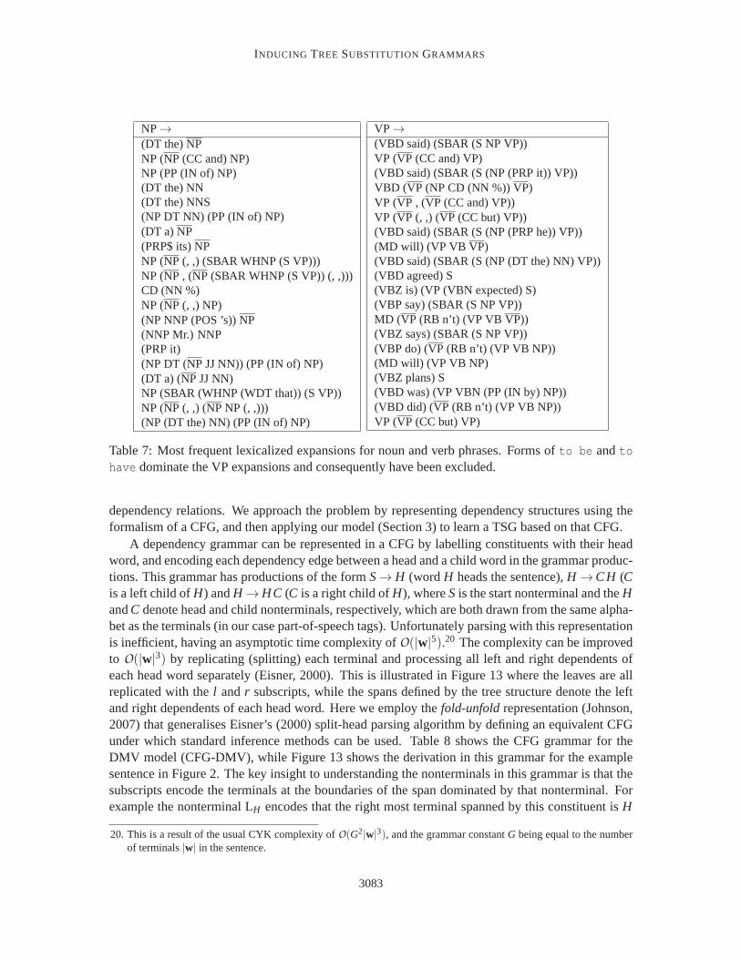
INDUCING TREE SUBSTITUTION GRAMMARS
NP→
(DT the)NPNP (NP (CC and) NP)NP (PP (IN of) NP)(DT the) NN(DT the) NNS(NP DT NN) (PP (IN of) NP)(DT a)NP(PRP$ its)NPNP (NP (, ,) (SBAR WHNP (S VP)))NP (NP , (NP (SBAR WHNP (S VP)) (, ,)))CD (NN %)NP (NP (, ,) NP)(NP NNP (POS ’s))NP(NNP Mr.) NNP(PRP it)(NP DT (NP JJ NN)) (PP (IN of) NP)(DT a) (NP JJ NN)NP (SBAR (WHNP (WDT that)) (S VP))NP (NP (, ,) (NP NP (, ,)))(NP (DT the) NN) (PP (IN of) NP)
VP →(VBD said) (SBAR (S NP VP))VP (VP (CC and) VP)(VBD said) (SBAR (S (NP (PRP it)) VP))VBD (VP (NP CD (NN %))VP)VP (VP , (VP (CC and) VP))VP (VP (, ,) (VP (CC but) VP))(VBD said) (SBAR (S (NP (PRP he)) VP))(MD will) (VP VB VP)(VBD said) (SBAR (S (NP (DT the) NN) VP))(VBD agreed) S(VBZ is) (VP (VBN expected) S)(VBP say) (SBAR (S NP VP))MD (VP (RB n’t) (VP VB VP))(VBZ says) (SBAR (S NP VP))(VBP do) (VP (RB n’t) (VP VB NP))(MD will) (VP VB NP)(VBZ plans) S(VBD was) (VP VBN (PP (IN by) NP))(VBD did) (VP (RB n’t) (VP VB NP))VP (VP (CC but) VP)
Table 7: Most frequent lexicalized expansions for noun and verb phrases. Forms ofto be andtohave dominate the VP expansions and consequently have been excluded.
dependency relations. We approach the problem by representing dependency structures using theformalism of a CFG, and then applying our model (Section 3) to learn a TSG based on that CFG.
A dependency grammar can be represented in a CFG by labelling constituentswith their headword, and encoding each dependency edge between a head and a childword in the grammar produc-tions. This grammar has productions of the formS→ H (wordH heads the sentence),H →CH (Cis a left child ofH) andH →HC (C is a right child ofH), whereSis the start nonterminal and theHandC denote head and child nonterminals, respectively, which are both drawn from the same alpha-bet as the terminals (in our case part-of-speech tags). Unfortunately parsing with this representationis inefficient, having an asymptotic time complexity ofO(|w|5).20 The complexity can be improvedto O(|w|3) by replicating (splitting) each terminal and processing all left and right dependents ofeach head word separately (Eisner, 2000). This is illustrated in Figure 13where the leaves are allreplicated with thel andr subscripts, while the spans defined by the tree structure denote the leftand right dependents of each head word. Here we employ thefold-unfoldrepresentation (Johnson,2007) that generalises Eisner’s (2000) split-head parsing algorithm bydefining an equivalent CFGunder which standard inference methods can be used. Table 8 shows theCFG grammar for theDMV model (CFG-DMV), while Figure 13 shows the derivation in this grammar for the examplesentence in Figure 2. The key insight to understanding the nonterminals in thisgrammar is that thesubscripts encode the terminals at the boundaries of the span dominated by that nonterminal. Forexample the nonterminal LH encodes that the right most terminal spanned by this constituent isH
20. This is a result of the usual CYK complexity ofO(G2|w|3), and the grammar constantG being equal to the numberof terminals|w| in the sentence.
3083
COHN, BLUNSOM AND GOLDWATER
(and the reverse forHR), whileAMB encodes thatA andB are the left and right terminals of the span.The superscripts∗ and1 denote the valency of the head: both indicate that the head has at least oneattached dependent in the specified direction, with1 indicating that the head will continue to attachmore children. The time complexity of inference in this grammar is onlyO(|w|3) because each spanin the parse chart bounded by terminals A and B can only contain nonterminallabels from the set{LB, L∗
B, L1B, AR, AR∗, AR1, AMB∗ , A∗MB, S}. Consequently the grammar constant is fixed rather
than quadratic in the sentence length.We apply our TSG model to unsupervised dependency grammar induction using the CFG-DMV
as the underlying grammar representation. Our model is capable of learningtree fragments whichcombine multiple adjacent CFG productions, affording considerable additional modelling powerabove that of a PCFG. Thereby the model can learn to condition dependency links on the valence.For example by combining LNN → L1
NN and L1NN → LDT DTMNN∗ rules into an elementary tree the
model can describe that the leftmost child of a noun (NN) is a determiner (DT). Moreover, themodel can learn groups of dependencies that occur together by conjoining multiple L1
H or HR1
nonterminals. This can represent, for example, the complete preferred argument frame of a verb.
7.1 Experiments
We perform inference for the TSG-DMV model by drawing 1000 samples using the blockedMetropolis-Hastings sampler described in Section 4.2 and evaluate the model using the final sam-ple. Given that we do not observe parse trees in training, we cannot use the local Gibbs sampler asit only allows the sampling of the segmentation of a fixed tree, not the tree itself. In order to parsesentences in the test set we use the Viterbi algorithm to find the maximum probability parse underthe MAP grammar (see Section 5). All hyperparameters,a,b ands, are sampled after every ten fullsamples over the training set.
A final and important consideration is the initialisation of the sampler. Klein and Manning(2004) emphasised the importance of the initialiser for achieving good performance with theirmodel. We employ Klein and Manning’sharmonic initialiser which defines a PCFG in whichall words have the same valency distribution and probability of being the sentence head, while theprobability of a head word attaching to a child word is inversely proportionalto the average distancebetween these words in the training corpus. To obtain the initial derivations for the sampler we takethe Viterbi derivations under this PCFG.
We follow the standard evaluation regime for DMV style models by performing experimentson the text of the WSJ section of the Penn. Treebank (Marcus et al., 1993). The corpus statisticsare reported in Table 9. Like previous work we pre-process the trainingand test data to remove thewords and punctuation, training our models on the gold-standard part-of-speech tags.
It is difficult for an unsupervised model to learn from long training sentences as their structureis highly ambiguous, and therefore the majority of DMV based approaches have been trained onsentences restricted in length to≤ 10 tokens. This has the added benefit of decreasing the runtimefor experiments. We present experiments with this training scenario, plus anadditional experimentwhere we increase the length cutoff to≤ 15. For the≤ 15 experiment we start by sampling onlysentences up to length 10, then gradually relax this length cutoff until we aresampling all sentencesup to length 15 after 900 samples.21 The training data is taken from sections 2-21, while section 23 isused for evaluation (see Table 9). An advantage of our sampling based approach over previous work
21. This training method is similar in spirit to the Baby Steps algorithm (Spitkovsky et al., 2010).
3084

INDUCING TREE SUBSTITUTION GRAMMARS
CFG Rule DMV Distribution Description
S→ LH HR p(root = H) The head of the sentence isH.
LH → Hl p(STOP|dir = L,head= H,val = 0) H has no left children.LH → L1
H p(CONT|dir = L,head= H,val = 0) H has at least one left child.
L∗H → Hl p(STOP|dir = L,head= H,val = 1) H has no more left children.
L∗H → L1
H p(CONT|dir = L,head= H,val = 1) H has another left child.
HR → Hr p(STOP|dir = R,head= H,val = 0) H has no right children.HR → HR1 p(CONT|dir = R,head= H,val = 0) H has at least one right child.
HR∗ → Hr p(STOP|dir = R,head= H,val = 1) H has no more right children.HR∗ → HR1 p(CONT|dir = R,head= H,val = 1) H has another right child.
L1H → LC CMH∗ p(C|dir = L,head= H) C is a left child ofH.
HR1 → H∗MC CR p(C|dir = R,head= H) C is a right child ofH.
CMH∗ → CR L∗H p= 1 Structural rule.
H∗MC → HR∗ LC p= 1 Structural rule.
Table 8: The CFG-DMV grammar schema. Note that the actual CFG is created by instantiatingthese templates with part-of-speech tags observed in the data for the variables H and C. Valency(val) can take the value 0 (no attachment in directiondir) and 1 (one or more attachment). L and Rindicates child dependents left or right of the parent; superscripts encode the stopping and valencydistributions, X1 indicates that the head will continue to attach more children and X∗ that it hasalready attached a child.
S
Lhates
L1hates
LGeorge
Georgel
GeorgeMhates∗
GeorgeR
Georger
L∗hates
hatesl
hatesR
hatesR1
hates∗Mbroccoli
hatesR∗
hatesr
Lbroccoli
broccolil
broccoliR
broccolir
Figure 13: The CFG-DMV derivation for the example sentenceGeorge hates broccoli. The depen-dency parse for this sentence is given in Figure 2.
3085

COHN, BLUNSOM AND GOLDWATER
Partition Sections Words Sentences
training≤10 2–21 42505 6007training≤15 2–21 132599 12880development≤10 22 1805 258test≤10 23 2649 398test≤15 23 16591 1286test≤∞ 23 49368 2416
Table 9: Corpus statistics for the training and testing data for the TSG-DMV model. All models aretrained on the gold standard part-of-speech tags after removing punctuation.
is that we infer all the hyperparameters; consequently there is no need to tune on the developmentset (section 22).
The models are evaluated in terms of head attachment accuracy (the percentage of correctlypredicted head dependency links for each token in the test data), on three subsets of the testing data.Although unsupervised models are better learnt from a corpus of shortrather than long sentences,they must still be able to parse long sentences. The most commonly employed testset mirrors thetraining data by only including sentences≤ 10, however we also include results for sentences≤ 20and the whole test set with no length restriction. As we are using MCMC samplingthe result of anysingle run is non-deterministic and will exhibit a degree of variance. Our reported results are themean and standard deviation (σ) from 40 sampling runs.
7.2 Discussion
Table 10 shows the head attachment accuracy results for our TSG-DMV,along with those of severalother competitive models. Our model performs very well in comparison to the others; in particular itachieves the highest reported accuracy on the full test set by a considerable margin. On the|w| ≤ 10test set the TSG-DMV is second only to the L-EVG model of Headden III etal. (2009). The L-EVG model extends DMV by adding additional lexicalisation, valency conditioning, interpolatedback-off smoothing and a random initialiser. In particular Headden III etal. show that the randominitialiser is crucial for good performance, but their approach requirestraining 1000 models toselect a single best model for evaluation and leads to considerable variance in test set performance.Our model exhibits considerably less variance than those induced using thisrandom initialiser,suggesting that the combination of the harmonic initialiser and blocked MH samplingmay be amore practical training regime. The recently-proposed Adaptor Grammar DMV model of Cohenet al. (2010) is similar in many ways to our TSG model, incorporating a Pitman Yor prior overunits larger than CFG rules. As such it is surprising that our model performs significantly betterthan this model. We can identify a number of possible explanations for these results: the AdaptorGrammar model is trained using variational inference with the space of tree fragments truncated,while we employ a sampler which can nominally explore the full space of tree fragments; and thetree fragments in the Adaptor Grammar model must be complete subtrees (i.e., theydon’t containvariables), whereas our model can make use of arbitrary tree fragments. An interesting avenue forfurther research would be to extend the variational algorithm of Cohen etal. (2010) to our TSG
3086

INDUCING TREE SUBSTITUTION GRAMMARS
Directed Attachment Accuracy% on Section 23
Model Initialiser |w| ≤ 10 |w| ≤ 20 |w| ≤ ∞
Attach-Right - 38.4 33.4 31.7
EM (Klein and Manning, 2004) Harmonic 46.1 39.9 35.9Dirichlet (Cohen et al., 2009) Harmonic 46.1 40.6 36.9
LN (Cohen et al., 2009) Harmonic 59.4 45.9 40.5SLN, TIE V&N (Cohen and Smith, 2009) Harmonic 61.3 47.4 41.4
DMV (Headden III et al., 2009) Random 55.7σ=8.0 - -DMV smoothed(Headden III et al., 2009) Random 61.2σ=1.2 - -EVG smoothed(Headden III et al., 2009) Random 65.0σ=5.7 - -L-EVG smoothed(Headden III et al., 2009) Random 68.8σ=4.5 - -
Less is More WSJ15(Spitkovsky et al., 2010) Harmonic 56.2 48.2 44.1Leap Frog WSJ45(Spitkovsky et al., 2010) Harmonic 57.1 48.7 45.0
Adaptor Grammar(Cohen et al., 2010) Harmonic 50.2 - -
TSG-DMV Harmonic 65.9σ=2.4 58.3σ=2.3 53.1σ=2.4
TSG-DMV WSJ15 Harmonic 66.4σ=1.7 58.5σ=1.7 53.4σ=1.8
Supervised MLE(Cohen and Smith, 2009) - 84.5 74.9 68.8
Table 10: Head attachment accuracy for our two TSG-DMV models (highlighted), and many otherhigh performing models.
3087

COHN, BLUNSOM AND GOLDWATER
Tag Frequency Accuracy Tag Frequency Accuracy
NN 564 0.70 CC 62 0.77NNP 366 0.67 VBG 48 0.71NNS 302 0.74 POS 26 0.92DT 292 0.81 MD 22 0.82IN 292 0.59 JJR 20 0.60JJ 266 0.67 PRP$ 18 1.00VBD 266 0.79 EX 12 1.00CD 224 0.21 WP 12 0.17RB 212 0.40 JJS 10 0.40PRP 132 0.94 WDT 6 1.00VBZ 118 0.88 RP 6 0.33VBN 84 0.71 RBS 4 1.00VBP 78 0.67 UH 4 0.50TO 70 0.43
Table 11: Head attachment accuracy stratified by child tag, as measured onthe held-out developmentset (WSJ 22,|w| ≤ 10). The tags are sorted by frequency.
model, possibly improving inference time while also allowing for the implementation to bemoreeasily parallelised.
To illustrate the kinds of structures the model induces and the types of errors it makes, Figure14 presents a representative example tree for a sentence from Section 22 of the WSJ. Though manyof the elementary trees in this example resist an obvious linguistic explanation, on the right sideof the derivation (highlighted in green) we see that the model has learnt to encode that the verbtakes a single noun phrase as its object, while on the left (highlighted in blue) isa rule specifyingthe DT JJ subject dependent of the VBZ. This derivation is typical of the analyses produced bythe model as it contains a number of dependency links which are inconsistent with the treebank.However we can see that the model has learnt to analyse the noun, verb and preposition phrases in amanner which is quite plausible, despite not matching the reference tree. In particular there wouldseem to be little obvious reason to prefer the treebank’s analysis of the conjunction phrase (‘eitherapathy or civility’) over that produced by the unsupervised model. This highlights the difficulty inevaluating the output of unsupervised grammar induction algorithms against atreebank reference;in this instance it is clear that the analysis found by the model, despite its low accuracy, could bevery useful for a downstream NLP application reliant on a dependencyanalysis.
For further analysis Tables 11 and 12 show the accuracy of the model at predicting the headfor each tag type and the accuracy for dependencies spanning a given number of tokens. Clearlythe model is far more accurate when predicting short dependencies, a result that is also reflectedin the per-tag results. We also note that the model accurately predicts the head of the sentence84% of the time, indicating an ability to capture the high level sentence structure.As mentionedabove, conjunctions pose a particular difficulty with unsupervised models as the correct modellingof these remains a contentious linguistic issue. Nevertheless on conjunctionsthe model does achievea reasonable level of agreement with the treebank.
3088

INDUCING TREE SUBSTITUTION GRAMMARS
(a) TSG-DMV representation. Large bold nodes indicate substitution points.
S
LV BZ
L1
V BZ
LDT
DTl
DT MV BZ∗
DT R
DT R1
DT∗MJJ
DT R∗
DTr
LJJ
JJl
JJR
JJr
L∗
V BZ
VBZl
V BZR
V BZR1
V BZ∗MNN
V BZR∗
VBZr
LNN
L1
NN
LDT
DTl
DT MNN∗
DT R
DTr
L∗
NN
NNl
NNR
NN R1
NN∗MIN
NNR∗
NNr
LIN
INl
IN R
INR1
IN∗MNN
IN R∗
INr
LNN
L1
NN
LNN
L1
NN
LDT
DTl
DT MNN∗
DT R
DTr
L∗
NN
NNl
NN MNN∗
NNR
NNR1
NN∗MCC
NNR∗
NNr
LCC
CCl
CCR
CCr
L∗
NN
NNl
NN R
NNr
(b) Dependency tree representation. The red links below the sentence show where the treebank reference analysis differsfrom the predicted tree.
The above represents a triumph of either apathy or civility
ROOT
Figure 14: An example induced tree, shown as an elementary tree (a) and as a dependency tree (b).The sentence was taken from the development set:"The DT above JJ represents VBZ aDT triumph NN
of IN either DT apathy NN or CC civility NN" .
3089

COHN, BLUNSOM AND GOLDWATER
Link Distance Precision Recall F1-Score
ROOT 0.84 0.84 0.841 0.68 0.72 0.702 0.61 0.53 0.573 0.56 0.46 0.514 0.47 0.52 0.495 0.27 0.35 0.306 0.44 0.57 0.507 0.33 0.38 0.358 0.25 0.12 0.17
Table 12: Performance on dependency links of varying distance. Precision, recall and f-score on theWSJ Section 22 (|w| ≤ 10) held-out set.
TSG-DMV Rules Frequency
LNN → (LNN (L1NN LDT (DTMNN∗ DTR L∗
NN))) 906INR → (INR (INR1
IN∗MNN NNR)) 839S → (S (LVBD L1
VBD) VBDR) 707
JJMNN∗ → (JJMNN∗ JJR (L∗NN NNl )) 600
NN∗MNN → (NN∗MNN NNR∗ (LNN NNl )) 589L1
NN → (L1NN LDT (DTMNN∗ DTR L∗
NN)) 587LNNP → (LNNP (L1
NNP (LNNP NNPl ) NNPMNNP∗)) 540L∗
NN → (L∗NN (L1
NN LJJ JJMNN∗)) 500TO∗MVB → (TO∗MVB (TOR∗ TOr ) LVB) 437
NNR → (NNR (NNR1NN∗MNN (NNR NNr ))) 412
DTMNNS∗ → (DTMNNS∗ (DTR DTr ) L∗NNS) 397
INR → (INR (INR1IN∗MNNS(NNSR NNSr ))) 328
LNNS → (LNNS(L1NNSLDT DTMNNS∗)) 326
INMCD∗ → (INMCD∗ (INR INr ) (L∗CD CDl )) 302
NNSMVBD∗ → (NNSMVBD∗ (NNSR NNSr ) L∗VBD) 296
Table 13: The fifteen most frequent TSG-DMV rules in the training data.
3090

INDUCING TREE SUBSTITUTION GRAMMARS
Table 13 lists the most frequent TSG rules learnt by the model. The most frequent rule at the topof the table models noun phrases, encoding the fact that determiners haveno children and attach asa left child to a phrase headed by a noun. It is interesting to see that our model has used a TSG ruleto analyse noun phrases in a way consistent with the treebank, whereas the original DMV modelpreferred the opposite analysis of having DTs as the heads of noun phrases (Klein and Manning,2004). Both results could be supported from a linguistic standpoint (Abney, 1987), but neverthelessit is a notable outcome that our more powerful model prefers to head noun phrases with nouns.Further down the table we see another interesting rule:TO∗MVB → (TO∗MVB (TOR∗ TOr ) LVB). Thisrule specifies that a verb phrase headed by an infinitive attaches as the first child of the particletoon its left. Here the model has used the tree fragment to encode that the verbmust be the first rightchild of the particle, an analysis both consistent with the treebank and expressing a bias against anyform of split infinitive construction.
8. Conclusion
In this work we have presented a non-parametric Bayesian model for inducing tree substitutiongrammars in both supervised and unsupervised settings. By incorporatinga structured prior overelementary rules our model is able to reason over the infinite space of all such rules, producingcompact and simple grammars. In doing so, our model learns local structures for latent linguisticphenomena, such as verb subcategorisation and lexical agreement.
Our experimental results indicate that our model holds significant potential for a range of gram-mar induction tasks. In experiments using a treebank for training, we showed that the induced TSGgrammars strongly out-perform standard PCFGs, and are comparable to astate-of-the-art parser onsmall data samples. While our results when training on the full treebank are well shy of the bestavailable parsers, we have proposed a number of improvements to the model and the parsing algo-rithm that could lead to state-of-the-art performance in the future. Our second set of experimentsremoved the reliance on a treebank and showed that our TSG model achieves performance similarto the best recent models on sentences up to length 10, and outperforms allother models on longersentences. This result is particularly promising, since it demonstrates the possibility of successfullylearning complex hierarchical models, beyond just CFGs, without supervision. We hope that ourwork will open the door to further research into inducing linguistically rich grammars, such as treeadjoining and categorial grammars, that have so far been considered toodifficult to learn from rawstrings.
References
Steven Paul Abney.The English Noun Phrase in its Sentential Aspect. PhD thesis, MassachusettsInstitute of Technology, Cambridge, Massachusetts, 1987.
David Aldous. Exchangeability and related topics. InEcole d’ete de probabilites de Saint-Flour,XIII—1983, pages 1–198. Springer, Berlin, 1985.
Phil Blunsom and Trevor Cohn. Unsupervised induction of tree substitution grammars for de-pendency parsing. InProceedings of the 2010 Conference on Empirical Methods in NaturalLanguage Processing, pages 1204–1213, Boston, Massachusetts, October 2010.
3091

COHN, BLUNSOM AND GOLDWATER
Rens Bod. Using an annotated language corpus as a virtual stochastic grammar. In11th NationalConference on Artificial Intelligence, pages 778–783, Washington D.C., USA, July 1993.
Rens Bod. The problem of computing the most probable tree in data-orientedparsing and stochastictree grammars. InProceedings of the 7th conference on European chapter of the Association forComputational Linguistics, pages 104–111, Dublin, Ireland, 1995.
Rens Bod. Combining semantic and syntactic structure for language modeling.In Proceedingsof the 6th International Conference on Spoken Language Processing, pages 106–109, Beijing,China, 2000.
Rens Bod. An efficient implementation of a new DOP model. InProceedings of the 10th Conferenceof the European Chapter of the Association for Computational Linguistics, Budapest, Hungary,April 2003.
Rens Bod. An all-subtrees approach to unsupervised parsing. InProceedings of the 21st Interna-tional Conference on Computational Linguistics and 44th Annual Meeting ofthe Association forComputational Linguistics, pages 865–872, Sydney, Australia, July 2006.
Rens Bod, Remko Scha, and Khalil Sima’an, editors.Data-oriented parsing. Center for the Studyof Language and Information — Studies in Computational Linguistics. University of ChicagoPress, 2003.
Glenn Carroll and Eugene Charniak. Two experiments on learning probabilistic dependency gram-mars from corpora. InProceedings of the AAAI Workshop on Statistically-Based Natural Lan-guage Processing Techniques, San Jose, California, 1992.
Eugene Charniak and Mark Johnson. Coarse-to-fine n-best parsing and maxent discriminativereranking. InProceedings of the 43rd Annual Meeting of the Association for ComputationalLinguistics, pages 173–180, Ann Arbor, Michigan, June 2005.
David Chiang and Daniel M. Bikel. Recovering latent information in treebanks. InProceedings ofthe 19th International Conference on Computational Linguistics, pages 183–189, Taipei, Taiwan,2002.
Alexander Clark. Unsupervised induction of stochastic context-free grammars using distributionalclustering. InProceedings of the 2001 workshop on Computational Natural Language Learning,pages 1–8, Toulouse, France, 2001.
Shay B. Cohen and Noah A. Smith. Shared logistic normal distributions for soft parameter tyingin unsupervised grammar induction. InProceedings of Human Language Technologies: The2009 Annual Conference of the North American Chapter of the Association for ComputationalLinguistics, pages 74–82, 2009.
Shay B. Cohen, Kevin Gimpel, and Noah A. Smith. Logistic normal priors for unsupervised prob-abilistic grammar induction. In Daphne Koller, Dale Schuurmans, Yoshua Bengio, and LonBottou, editors,Advances in Neural Information Processing Systems 21, pages 321–328. 2009.
3092

INDUCING TREE SUBSTITUTION GRAMMARS
Shay B. Cohen, David M. Blei, and Noah A. Smith. Variational inference for adaptor grammars. InHuman Language Technologies: The 11th Annual Conference of the North American Chapter ofthe Association for Computational Linguistics, pages 564–572, 2010.
Trevor Cohn and Phil Blunsom. Blocked inference in Bayesian tree substitution grammars. InProceedings of the ACL 2010 Conference Short Papers, pages 225–230, Uppsala, Sweden, July2010.
Trevor Cohn, Sharon Goldwater, and Phil Blunsom. Inducing compact but accurate tree-substitutiongrammars. InProceedings of Human Language Technologies: The 2009 Annual Conference ofthe North American Chapter of the Association for Computational Linguistics, pages 548–556,Boulder, Colorado, June 2009.
Jason Eisner. Bilexical grammars and their cubic-time parsing algorithms. In Harry Bunt and AntonNijholt, editors,Advances in Probabilistic and Other Parsing Technologies, pages 29–62. KluwerAcademic Publishers, October 2000.
Thomas S. Ferguson. A bayesian analysis of some nonparametric problems. Annals of Statistics,1(2):209–230, 1973.
Jenny Rose Finkel, Trond Grenager, and Christopher D. Manning. The infinite tree. InProceedingsof the 45th Annual Meeting of the Association of Computational Linguistics, pages 272–279,Prague, Czech Republic, June 2007.
Stuart Geman and Donald Geman. Stochastic relaxation, Gibbs distributions and the Bayesianrestoration of images.IEEE Transactions on Pattern Analysis and Machine Intelligence, 6:721–741, 1984.
E. Mark Gold. Language identification in the limit.Information and Control, 10(5):447–474, 1967.
Sharon Goldwater, Thomas L. Griffiths, and Mark Johnson. Contextualdependencies in unsuper-vised word segmentation. InProceedings of the 21st International Conference on ComputationalLinguistics and 44th Annual Meeting of the Association for Computational Linguistics, pages673–680, Sydney, Australia, July 2006.
Joshua Goodman.Parsing Inside-Out. PhD thesis, Harvard University, 1998.
Joshua Goodman. Efficient parsing of DOP with PCFG-reductions. In Bod et al. (2003), chapter 8.
William P. Headden III, Mark Johnson, and David McClosky. Improving unsupervised dependencyparsing with richer contexts and smoothing. InProceedings of Human Language Technologies:The 2009 Annual Conference of the North American Chapter of the Association for Computa-tional Linguistics, pages 101–109, Boulder, Colorado, June 2009.
Hemant Ishwaran and Lancelot F. James. Generalized weighted Chineserestaurant processes forspecies sampling mixture models.Statistica Sinica, 13:1211–1235, 2003.
Mark Johnson. The DOP estimation method is biased and inconsistent.Computational Lingusitics,28(1):71–76, March 2002.
3093

COHN, BLUNSOM AND GOLDWATER
Mark Johnson. Transforming projective bilexical dependency grammars into efficiently-parsablecfgs with unfold-fold. InProceedings of the 45th Annual Meeting of the Association of Compu-tational Linguistics, pages 168–175, Prague, Czech Republic, June 2007.
Mark Johnson. Using adaptor grammars to identify synergies in the unsupervised acquisition oflinguistic structure. InProceedings of ACL-08: HLT, pages 398–406, Columbus, Ohio, June2008a.
Mark Johnson. Unsupervised word segmentation for Sesotho using adaptor grammars. InPro-ceedings of the Tenth Meeting of ACL Special Interest Group on Computational Morphology andPhonology, pages 20–27, Columbus, Ohio, June 2008b.
Mark Johnson and Sharon Goldwater. Improving nonparameteric bayesian inference: experimentson unsupervised word segmentation with adaptor grammars. InProceedings of Human LanguageTechnologies: The 2009 Annual Conference of the North American Chapter of the Associationfor Computational Linguistics, pages 317–325, Boulder, Colorado, June 2009.
Mark Johnson, Thomas Griffiths, and Sharon Goldwater. Bayesian inference for PCFGs via Markovchain Monte Carlo. InProceedings of Human Language Technologies 2007: The Conference ofthe North American Chapter of the Association for Computational Linguistics, pages 139–146,Rochester, NY, April 2007a.
Mark Johnson, Thomas L. Griffiths, and Sharon Goldwater. Adaptor grammars: A frameworkfor specifying compositional nonparametric Bayesian models. In B. Scholkopf, J. Platt, andT. Hoffman, editors,Advances in Neural Information Processing Systems 19, pages 641–648.2007b.
Aravind Joshi. Tree adjoining grammars. In Ruslan Mikkov, editor,The Oxford Handbook ofComputational Linguistics, pages 483–501. Oxford University Press, Oxford, England, 2003.
Dan Klein and Christopher D. Manning. A generative constituent-context model for improvedgrammar induction. InProceedings of 40th Annual Meeting of the Association for ComputationalLinguistics, pages 128–135, Philadelphia, Pennsylvania, USA, July 2002.
Dan Klein and Christopher D. Manning. Corpus-based induction of syntactic structure: models ofdependency and constituency. InProceedings of the 42nd Annual Meeting on Association forComputational Linguistics, pages 478–485, 2004.
Karim Lari and Steve J. Young. The estimation of stochastic context-free grammars using theinside-outside algorithm.Computer Speech and Language, 4:35–56, 1990.
Percy Liang, Slav Petrov, Michael Jordan, and Dan Klein. The infinite PCFG using hierarchi-cal Dirichlet processes. InProceedings of the 2007 Joint Conference on Empirical Methods inNatural Language Processing and Computational Natural Language Learning, pages 688–697,Prague, Czech Republic, June 2007.
Percy Liang, Michael I. Jordan, and Dan Klein. Type-based mcmc. InHuman Language Tech-nologies: The 2010 Annual Conference of the North American Chapter of the Association forComputational Linguistics, pages 573–581, Los Angeles, California, June 2010.
3094

INDUCING TREE SUBSTITUTION GRAMMARS
Mitchell P. Marcus, Mary Ann Marcinkiewicz, and Beatrice Santorini. Building a large annotatedcorpus of English: the Penn treebank.Computational Linguistics, 19(2):313–330, 1993.
Igor′ A. Mel′cuk. Dependency Syntax: Theory and Practice. State University of New York Press,Albany, 1988.
Bernard Merialdo. Tagging English text with a probabilistic model.Computational Linguistics, 20(2):155–172, 1994.
Radford Neal. Slice sampling.Annals of Statistics, 31:705–767, 2003.
Timothy J. O’Donnell, Noah D. Goodman, and Joshua B. Tenenbaum. Fragment grammar: Ex-ploring reuse in hierarchical generative processes. Technical Report MIT-CSAIL-TR-2009-013,MIT, 2009.
Slav Petrov. Products of random latent variable grammars. InHuman Language Technologies: The2010 Annual Conference of the North American Chapter of the Association for ComputationalLinguistics, pages 19–27, Los Angeles, California, June 2010.
Slav Petrov and Dan Klein. Improved inference for unlexicalized parsing. In Proceedings of HumanLanguage Technologies 2007: The Conference of the North American Chapter of the Associationfor Computational Linguistics, pages 404–411, Rochester, NY, April 2007.
Slav Petrov, Leon Barrett, Romain Thibaux, and Dan Klein. Learning accurate, compact, and inter-pretable tree annotation. InProceedings of the 21st International Conference on ComputationalLinguistics and 44th Annual Meeting of the Association for Computational Linguistics, pages433–440, Sydney, Australia, July 2006.
Jim Pitman. Exchangeable and partially exchangeable random partitions.Probability Theory andRelated Fields, 102:145–158, 1995.
Jim Pitman.Combinatorial Stochastic Processes. Springer-Verlag, New York, 2006.
Jim Pitman and Marc Yor. The two-parameter Poisson-Dirichlet distribution derived from a stablesubordinator.Annals of Probability, 25:855–900, 1997.
Matt Post and Daniel Gildea. Bayesian learning of a tree substitution grammar. In Proceedings ofthe ACL-IJCNLP 2009 Conference Short Papers, pages 45–48, Suntec, Singapore, August 2009.
Detlef Prescher, Remko Scha, Khalil Sima’an, and Andreas Zollmann. On the statistical consistencyof DOP estimators. InProceedings of the 14th Meeting of Computational Linguistics in theNetherlands, Antwerp, Belgium, 2004.
Valentin I. Spitkovsky, Hiyan Alshawi, and Daniel Jurafsky. From BabySteps to Leapfrog: How“Less is More” in unsupervised dependency parsing. InHuman Language Technologies: The11th Annual Conference of the North American Chapter of the Associationfor ComputationalLinguistics, pages 751–759, 2010.
Fei Xia. Automatic grammar generation from two different perspectives. PhD thesis, University ofPennsylvania, 2002.
3095

COHN, BLUNSOM AND GOLDWATER
Andreas Zollmann and Khalil Sima’an. A consistent and efficient estimator for data-oriented pars-ing. Journal of Automata, Languages and Combinatorics, 10(2):367–388, 2005.
Willem Zuidema. Parsimonious data-oriented parsing. InProceedings of the 2007 Joint Conferenceon Empirical Methods in Natural Language Processing and Computational Natural LanguageLearning, pages 551–560, Prague, Czech Republic, June 2007.
3096