
Inducing Clean Technology in the Electricity Sector: Tradable Permits or...
26
149 The Energy Journal, Vol. 32, No. 3. Copyright 2011 by the IAEE. All rights reserved. * Corresponding author. School of Social Sciences, Humanities and Arts, and School of Engi- neering, University of California, Merced, 5200 N. Lake Rd., Merced, CA 95348, USA. E-mail: [email protected] ** University of New South Wales, Australian School of Business, Sydney NSW 2052, Australia. E-mail: [email protected] Inducing Clean Technology in the Electricity Sector: Tradable Permits or Carbon Tax Policies? Yihsu Chen* and Chung-Li Tseng** Tradable permits and carbon taxes are two market-based instruments commonly considered by policymakers to regulate pollutions. While a tax is fixed, predetermined by authorities, the uncertain permits price is driven by market dynamics, fluctuating with the prices of natural gas and electricity. Both instru- ments offer firms different incentives for adopting clean technologies. This paper explores the optimal investment timing when a coal-fired plant owner considers introducing clean technologies in face of these two policies using a real options approach. We find that tradable permits could effectively trigger adopting clean technologies at a considerably lower level of carbon price relative to a tax policy. Higher levels of volatility in permit prices are likely to induce suppliers to take early actions to hedge against carbon risks. Thus, offset and other price control mechanisms, which are designed to reduce permit prices or to suppress prices volatility, are likely to delay clean technology investments. 1. INTRODUCTION Climate Change is an unprecedented challenge faced by our society to- day. The Fourth Assessment Report (AR4), released by the IPCC (Intergovern- mental Panel on Climate Change) in 2007, indicates that the link between the increase of greenhouse gases (GHG) in the atmosphere and global warming is evident by the trend of warming of the oceans, rising sea levels, widespread ice melting in the Arctic, etc (Intergovernmental Panel on Climate Change 2007). As the power sector constitutes one of the main sources of GHG, numerous resources and policies are expected to be devoted to controlling GHG emissions from the power and other energy-intensive sectors.
Transcript of Inducing Clean Technology in the Electricity Sector: Tradable Permits or...
149
The Energy Journal, Vol. 32, No. 3. Copyright �2011 by the IAEE. All rights reserved.
* Corresponding author. School of Social Sciences, Humanities and Arts, and School of Engi-neering, University of California, Merced, 5200 N. Lake Rd., Merced, CA 95348, USA. E-mail:[email protected]
** University of New South Wales, Australian School of Business, Sydney NSW 2052, Australia.E-mail: [email protected]
Inducing Clean Technology in the Electricity Sector: TradablePermits or Carbon Tax Policies?
Yihsu Chen* and Chung-Li Tseng**
Tradable permits and carbon taxes are two market-based instrumentscommonly considered by policymakers to regulate pollutions. While a tax is fixed,predetermined by authorities, the uncertain permits price is driven by marketdynamics, fluctuating with the prices of natural gas and electricity. Both instru-ments offer firms different incentives for adopting clean technologies. This paperexplores the optimal investment timing when a coal-fired plant owner considersintroducing clean technologies in face of these two policies using a real optionsapproach. We find that tradable permits could effectively trigger adopting cleantechnologies at a considerably lower level of carbon price relative to a tax policy.Higher levels of volatility in permit prices are likely to induce suppliers to takeearly actions to hedge against carbon risks. Thus, offset and other price controlmechanisms, which are designed to reduce permit prices or to suppress pricesvolatility, are likely to delay clean technology investments.
1. INTRODUCTION
Climate Change is an unprecedented challenge faced by our society to-day. The Fourth Assessment Report (AR4), released by the IPCC (Intergovern-mental Panel on Climate Change) in 2007, indicates that the link between theincrease of greenhouse gases (GHG) in the atmosphere and global warming isevident by the trend of warming of the oceans, rising sea levels, widespread icemelting in the Arctic, etc (Intergovernmental Panel on Climate Change 2007). Asthe power sector constitutes one of the main sources of GHG, numerous resourcesand policies are expected to be devoted to controlling GHG emissions from thepower and other energy-intensive sectors.
150 / The Energy Journal
1. Examples of technology standard include scrubbers and SNCRs (selective non-catalytic reduc-tion systems) for SO2 and NOx emissions from power plants.
Policy choice in combating climate change, like climate change itself,has been a longstanding debate. Two types of policies are generally implementedto control for pollution emissions: command-and-control and market-based in-struments. Command-and-control policies consist of technology and performancestandards, which mandate specific control technology to be installed and to stip-ulate emissions limits on emissions sources.1 Within the command-and-controlmechanism, performance standard grants owners the flexibility to decide theirpreferred technologies and tailor them to the design of their facilities. Industrywould favor the performance over the technology standard because of the flexi-bility, whereas government might incline to set the technology standard if thetransaction cost is substantially higher under performance standard.
While the market-based instrument is a generic label for various typesof environmental standards that take advantage of competition in the pollutingindustries, it generally refers to price and quantity instruments. The price instru-ment, commonly known as “tax,” acts as a cost adder internalizing pollutiondamage (i.e., “externality”) created by the polluting industries that is not fullyreflected in product prices. The second type regulates pollution quantity, or knownas “cap-and-trade” (C&T), which first allocates a fixed amount of emissions quan-tity (i.e., permits/allowances) to affected facilities. These facilities need to dem-onstrate their compliance by “surrendering” sufficient allowances to cover theiremissions at the end of each compliance cycle (e.g., the annual cap for SO2 andsummer months for NOx). The allowances can be traded freely in the secondarymarket. Under this approach, the aggregate cost for pollution control of a regu-lated sector (e.g., electricity) for a given reduction target is expected to be theleast if the market is competitive among other conditions (Stavins 1995). Theeconomic efficiency gains of the programs are due to heterogeneity in abatementcosts: companies with low control costs would control more, while their coun-terparts would purchase surplus allowances from them.
There is a rich body of literature comparing command-and-control andmarket-based instruments. Economists have long advocated for market-based ap-proaches on the grounds of economic efficiencies. A number of frequently citedadvantages of market-based instruments over command-and-control policies aresummarized as follows. First, a market based instrument results in an equalizationof marginal abatement costs across all polluters. This is a basic condition for aleast-cost outcome (i.e., static efficiency). Moreover, regulators do not need toknow the marginal abatement costs of the polluting industries, which normally isprivate information. Second, both C&T and tax instruments offer polluters incen-tives to undertake R&D (research and development) activities for exploring cost-saving abatement options (i.e., dynamic efficiency). Third, revenues raised by taxor permits auctions can be recycled, for instance by lowering other taxes and,hence, reducing distortions induced by pre-existing taxes (i.e.,double dividend)(Parry et al. 1997).
Inducing Clean Technology in the Electricity Sector / 151
2. For instance, it is estimated that 40–80% of the permits price of the European Union EmissionsTrading Scheme was passed on to electricity prices in 2005 (Sijm et al. 2006). Theoretically, the levelof CO2 pass-through costs depends on demand, supply elasticities, market competition, etc. If nochanges in the merit order for determining the marginal unit is assumed, the pass-through cost ispositively associated with supply elasticity, but is negatively associated with both demand elasticityand the number of firms in the market (Chen et al. 2008).
Although in theory these two market-based approaches, tax and permits,can result in the same outcomes if the tax is set to equal the marginal control/damage cost defined by the emission cap, fundamentally they offer firms distincteconomic incentives for investing in emission reductions. More specifically, thelevel of an emissions tax is pre-set by an authority and exogenous to the productmarket. As for emissions permits, producers might realize that permit prices fluc-tuate constantly, reflecting market participants’ expectations concerning demandand supply conditions. The permit prices could therefore be affected by changesof pivotal producers’ net positions in permits markets. For example, retrofittingpollution control devices or fuel-switch could lower the demand for permits,effectively suppressing permit prices.
Following the seminal work by Weitzman (1974), there is a rich bodyof literature comparing the performance of these two market-based instruments.For example, work by Mansur (2007) examines strategic behavior in an oligopolyelectricity market when producers are subject to either a tax or tradable permitsregulation. The results show that, unlike a tax, the polluters’ decisions under atradable permits system would affect the permit price, which might actually in-crease a strategic firm’s output, thereby leading to a lower deadweight loss relativeto a tax system. A more recent paper by Green (2008) examines market risksfaced by generators under the tax and permits systems. This paper concludes that,relative to a permits program, a carbon tax would reduce risk faced by nucleargenerators, but it would raise the risk associated with fossil-fired units. This canbe attributed to the fact that the permits price is closely correlated with fuel costs,and such a correlation further amplifies profit volatility faced by the fossil units.
However, to our knowledge, there is no formal treatment based on realoptions in the existing literature that compares the investment timing betweenthese two instruments. As in most competitive markets, the electricity price is setby the generating cost of the marginal unit, ignoring network congestion andother complications. The extent to which carbon costs (in the form of permitsand tax) would be passed on to the electricity price depends on the marginaltechnology, which differs by markets.2 Although both the carbon tax and permitcost will be passed onto the electricity price, their underlying economic force isdifferent, and their relation with respect to fuel costs, such as natural gas (NG),is distinct. In particular, the permit’s price, the electricity price, and the NG priceare idiosyncratic and are likely to be positively correlated. This is because anelevation of NG prices (e.g., due to shortage or other reasons) would increasecoal consumption because coal and NG are substitutable goods. This in turn would
152 / The Energy Journal
3. Economic theories define technological change by three consecutive stages: invention, inno-vation, and diffusion (Jaffe et al. 2002). Invention constitutes the initial conversion of scientific ortechnical knowledge into new products or processes. Innovation defines as the commercialization ofnew products or processes based on the invention and make them available to the public. Finally,diffusion refers to the adoption of products by firms or individuals. In this paper, the term “investment”refers to diffusion of a low-CO2 generating technology.
4. In fact, the correlation among these three prices depends on the generating mix in a market.When a market is competitive, a diversified generating portfolio that allows for a greater fuel substi-tution when facing permit prices would result in a strong correlation between fuel costs and electricityprices.
increase the demand of the permits and would induce a positive pressure on thepermit price, as well as the electricity price. On the contrary, the tax is determineda priori (or fixed) by the government and is insensitive to any market dynamics.
This paper studies the timing that a firm invests in a less CO2-intensivetechnology under some emission control policy. This is especially critical for afirm to mitigate the financial impacts resulting from climate policy. Because theimpact of climate change is irreversible, firms that take precautionary actions toreduce GHG emissions could have profound effects, but they may need to bearsubstantial investment costs. From the perspective of technology diffusion3, adesirable climate change policy should provide polluting industries with strongincentives to take early preventive actions. Several studies examined technologydiffusion under tax and C&T based on game-theoretical framework, e.g., seeMilliman and Price (1989), Kennedy and Lapiante (1999), Requate and Unold(2003), Coria (2009), Montero (2002a), and Montero (2002b). Their focus wason the comparison of incentives provided by different policy instruments. Ourpaper explores the timing of investment as a function of data-generating processesunderlying various prices using a real options approach.
We assume that a price-taking firm (who is small relative to the entiremarket) owns a coal plant (i.e., polluting energy resource) subject to load obli-gation and faces three exogenous price shocks: electricity, NG, and permits. Con-sidering two different policies, tax and C&T, we examine the timing under eachpolicy such that the firm adds an NG power plant (i.e., clean technology) in orderto meet the load obligation while maximizing its expected long-run profit withemission-related costs considered. Whereas the prices for electricity, permits, andNG are closely correlated in the emission trading system4, the level of tax man-dated by authorities is assumed completely independent from electricity and NGprices. We explore the relation of investment timing under each policy in termsof the price parameters. Although we focus on the choices of a new NG plant,the implication could be generalized to other decision contexts, such as retrofittingpollution control devices, carbon capture and storage (CCS), or other alternativesmitigating CO2 emissions.
In order to evaluate the profitability of capacity expansion, our modelfocuses on “operational” perspective of the policies in terms of the investmenttiming for inducing new technologies. First, the decision leadtime (e.g., the re-
Inducing Clean Technology in the Electricity Sector / 153
5. The unit is $/ton, since CO2 emission of a typical coal plant is roughly a ton per MWh gen-eration, however, it can also be approximated as $/MWh.
quired time for applying for permits and/or constructing the power plant) will bemodeled, and its impact on profitability and investment timing will be studied.In particular, we explore the effect of correlations among electricity, permits, andNG prices on the firm’s investment decisions. Second, we deploy a more realisticmodel that includes the firm’s ability to produce the power flexibly (by dispatch-ing both coal and NG units) based on price spreads.
The rest of this paper is organized as follows: In Section 2, an economicmodel is presented. A case analysis based on real price data used to illustrate ourresults is presented in Section 3. We conclude the paper in Section 4.
2. MODEL SETUPS
This section provides detailed model setups, including the uncertaintymodel, the problem formulation, the model interpretation, and the solution pro-cedure.
2.1 Uncertainty Model and Emission Policies
Three uncertainties are considered in this paper at day in the planningthorizon for : prices for electricity ($/MWh), natural gas ($/MMBtu),t�0 X Gt t
and emission permits ($/MWh)5. As already mentioned, we will consider twoYt
emission control policies in this paper: tradable permit and tax. The price foremission permits will be used in evaluating the policy of tradable permits.Yt
These three uncertainties are assumed to evolve following the geometric Brown-ian motions, for any time :s� t
xdX �l (X , s)ds�r dB (1a)s x s x s
ydY �l (Y , s)ds�r dB (1b)s y s y s
gdG �l (G , s)ds�r dB , (1c)s g s g s
where , , and are correlated Wiener processes such thatx y gB B Bs s s
x ydB dB �q ds (2a)s s xy
y gdB dB �q ds (2b)s s yg
g xdB dB �q ds (2c)s s gx
In equations (1a)–(1c), the price evolutions are assumed to follow some stochasticprocesses, where , , and are the drift functions for the processes, respec-l l lx y g
154 / The Energy Journal
6. Of course, one could add a stochastic coal price in the model. However, the curse of dimensionmight make computation much difficult. We believe our assumption is reasonable since the historicaldata also suggest that the costs of coal are considerably stable compared to NG prices (Sijm et al.2006).
tively, and , , are constant (but may be time dependent) volatilities. Assumer r rx y g
at time 0, the prices of , , and are , , and , respectively. That is,X Y G x y g0 0 0
(X , Y , G )�(x, y, g). (3)0 0 0
When the taxation policy is considered, is reduced to a constant by settingY Yt
. In this case, represents the tax payment and is time-invariant. Thel �r �0 Yy y
correlation terms and in equations (2a)–(2c) are also set to zero. Since theq qxy yg
constant may be viewed as a special (degenerate) case of , in the remainderY Yt
of the paper, our analysis will focus on valuation under these three uncertainties.
2.2 Problem Formulation: A Per MW Analysis
This section considers a decision problem concerning the capacity in-vestment faced by a risk-neutral price-taking producer who owns an existing coalplant. As the pressure for employing cleaner power-generating technologies ismounting, the producer considers to add a NG plant in the future. Of course,capacity additions could be driven by factors other than CO2 policy, such as easyaccess to capital, friendly regulatory environment, etc. However, we limit ouranalysis to situations exclusively related to CO2 policy. Currently with the existingcoal plant, the costs for generating one MWh electricity at include the cost oftcoal, assumed to be a constant ($/MWh)6, and the emission cost ($/MWh),C Yt
determined by the emission market. Therefore, for the existing coal plant the perMWh profit at time is denoted by as follows.0t ft
0f (X , Y )�X –C–Y , (4)t t t t t
where the superscript 0 implies no expansion yet.If an NG plant is built, using the NG plant to generate one MWh results
in a profit of at time , where is the NG price and (MMBtu/X –G H–0.5Y t G Ht t t t
MWh) is the heat rate of the plant. Since in general, an NG plant emits about halfof the CO2 emitted by a coal plant on a per MWh basis, the emission cost for theNG plant is set to be . We ignore the possibility of further reduction of CO20.5Yt
emissions from the NG plant by means of other advanced technology when theybecome available. With the new NG plant, the decision maker can generate powerby the portfolio of these two power plants. The dispatch of both power plantswill be conducted in a cost-minimizing manner. Therefore, the per MWh profitof the portfolio at takes the following form:t
Portfolio’s per MWh profit� (5)
max [(1–� )(X –C–Y )�� (X –G H–0.5Y )],t t t t t t t0� � � �t
Inducing Clean Technology in the Electricity Sector / 155
where is a dispatch factor at time and is between 0 and , which is a constant� t �t
representing the ratio of the capacity of the NG plant to that of the coal plant.Since in general the capacity of a coal plant is greater than that of an NG plant,
is assumed to be less than 1.�Recognizing that the portfolio profit in (5) is a linear function of the
prices, , , and , an optimal dispatch will only occur on the boundary points,X Y Gt t t
or . Therefore, the two possible dispatches correspond to either (i)� �0 � ��t t
the coal plant is fully on with the NG plant off ( ); or (ii) the NG plant is� �0t
fully on with the coal plant picking up the residue ( ) at time . Therefore,� �� tt
the (portfolio) profit function (5) at time can be summarized by the followingtfunction:
1f (X , Y , G )� max [(1–� )(X –C–Y )�� (X –G H–0.5Y )], (6)t t t t t t t t t t t� �{0, �}t
where the superscript 1 implies that expansion has occurred.Assume that the decision maker would build an NG plant at a future
time , which requires a capital investment of ($/MW), deposited at . Thes K sconstruction will need months to complete. The optimization involved in thismdecision making includes the optimal timing ( ) for building the NG plant, andsif so, the optimal dispatch ( ) between the existing coal plant and the new NG�t
plant.To focus on how emission policies induce the expansion decision for
building the NG plant, we assume the existing coal plant to be perpetual (but notthe NG plant). In reality, the coal plant’s life may be prolonged by regular, con-tinuous maintenance and upgrade. The reason for this assumption is more aca-demic than practical. We basically assume that the NG plant may come and go(built, operated, and retired); but the coal plant remains there. Since we are in-terested in finding the optimal timing to build the NG plant under different emis-sion policies, this assumption enables us to focus solely on the NG plant withoutworrying about possible retirement of the coal plant during the life cycle of theNG plant. This assumption also helps to reduce the complexity of the problem,which will become clear in Section 2.3.
Consider a decision period , within which a new NG plant ist� [0, T]expected to be added. The profit maximization for the decision maker of thisinvestment problem can be formulated as follows:
s�m0 – rs – rsJ(x, y, g)� max E [ f (X , Y )e ds–Ke0 s s s�
0s� [0, T]
�ls�m�1 – rs 0 – rs� f (X , Y , G )e ds� f (X , Y )e ds]. (7)s s s s s s s� �
s�m s�m�l
The optimization in (7) is subject to an additional constraint that the real optionof expansion expires after . In equation (7), it is clear that the NG plant is builtT
156 / The Energy Journal
at with a construction leadtime . After the completion of the construction, thes mNG plant has a life of time periods and after that will be disposed without anylsalvage value. Note that the optimization problem depends on the prices
at . The optimal (stopping) time to build is a random variable,(x, y, g) t�0 swhich is uncommitted at . Since we consider expansion as a real option, itt�0is possible that the expansion is never exercised during . Since the purpose[0, T]of this paper is to see how quickly an emission policy induces adoption of cleantechnology, for the instance where the expansion option expires without beingexercised, we will manually register its adoption time as , which is a largeTnumber ( months in our case study in Section 3). This enables us toT�120provide an expected waiting time for each scenario investigated. Therefore,E[s]when is large in our case study, it should just be interpreted as that expansionE[s]is highly unlikely within the finite horizon of .[0, T]
2.3 Real Options Perspectives
In our problem setup, the decision to build an NG power plant is clearlya real option of the decision maker. There are other less obvious real options tobe interpreted next.
First, equation (6) reveals a dispatch (or switching) real option for thedecision maker after the new NG plant has been built. The decision maker canobserve the prices and decide whether it is more profitable to generate the one-MW power using only the coal plant or both. To justify whether the NG plantshould be built, the overall value resulted from exercising the dispatch optionover the life time of the NG plant must be compared with the construction costof the plant, which may be viewed as the premium of having the dispatch realoptions.
To see the next real options interpretation, we rewrite the formulation inequation (7). With some algebra, equation (7) is equivalent to the following:
�– rs – rsJ(x, y, g)�E [ (X –C–Y )e ds]� max E [–Ke0 s s 0�
0 s� [0, T]
ls�m�– rs�� max(0.5Y �C–G H, 0)e ds]. (8)s s�
s�m
In equation (8), we separate the role that each plant plays. The firstintegral refers to the operation of the perpetual coal plant. The second integralreveals a spread option (e.g., see Carmona and Durrleman 2003) between andYt
with the payoff function . Interestingly, the electricityG max(0.5Y �C–G H, 0)t s s
price drops out of the payoff function. This is because the power output fromXt
either plant is indistinguishable and must add up to one MW. What matters is thedifference between the saving of the emission costs, , and the additional�(0.5Y )tcost for having the NG plant, .�(G H–C)t
Inducing Clean Technology in the Electricity Sector / 157
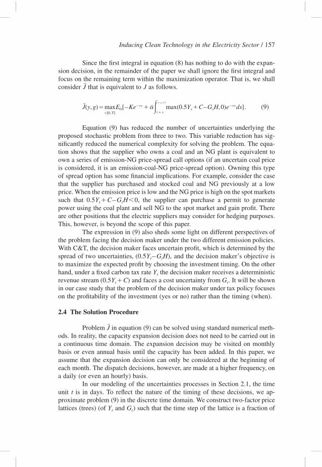
Since the first integral in equation (8) has nothing to do with the expan-sion decision, in the remainder of the paper we shall ignore the first integral andfocus on the remaining term within the maximization operator. That is, we shallconsider that is equivalent to as follows.J J
ls�m�– r – rssJ(y, g)�maxE [–Ke �� max(0.5Y �C–G H, 0)e ds]. (9)0 s s�
s�ms [0, T]
Equation (9) has reduced the number of uncertainties underlying theproposed stochastic problem from three to two. This variable reduction has sig-nificantly reduced the numerical complexity for solving the problem. The equa-tion shows that the supplier who owns a coal and an NG plant is equivalent toown a series of emission-NG price-spread call options (if an uncertain coal priceis considered, it is an emission-coal-NG price-spread option). Owning this typeof spread option has some financial implications. For example, consider the casethat the supplier has purchased and stocked coal and NG previously at a lowprice. When the emission price is low and the NG price is high on the spot marketssuch that , the supplier can purchase a permit to generate0.5Y �C–G H�0t t
power using the coal plant and sell NG to the spot market and gain profit. Thereare other positions that the electric suppliers may consider for hedging purposes.This, however, is beyond the scope of this paper.
The expression in (9) also sheds some light on different perspectives ofthe problem facing the decision maker under the two different emission policies.With C&T, the decision maker faces uncertain profit, which is determined by thespread of two uncertainties, and the decision maker’s objective is(0.5Y –G H),t t
to maximize the expected profit by choosing the investment timing. On the otherhand, under a fixed carbon tax rate the decision maker receives a deterministicYt
revenue stream and faces a cost uncertainty from . It will be shown(0.5Y �C) Gt t
in our case study that the problem of the decision maker under tax policy focuseson the profitability of the investment (yes or no) rather than the timing (when).
2.4 The Solution Procedure
Problem in equation (9) can be solved using standard numerical meth-Jods. In reality, the capacity expansion decision does not need to be carried out ina continuous time domain. The expansion decision may be visited on monthlybasis or even annual basis until the capacity has been added. In this paper, weassume that the expansion decision can only be considered at the beginning ofeach month. The dispatch decisions, however, are made at a higher frequency, ona daily (or even an hourly) basis.
In our modeling of the uncertainties processes in Section 2.1, the timeunit is in days. To reflect the nature of the timing of these decisions, we ap-tproximate problem (9) in the discrete time domain. We construct two-factor pricelattices (trees) (of and ) such that the time step of the lattice is a fraction ofY Gt t
158 / The Energy Journal
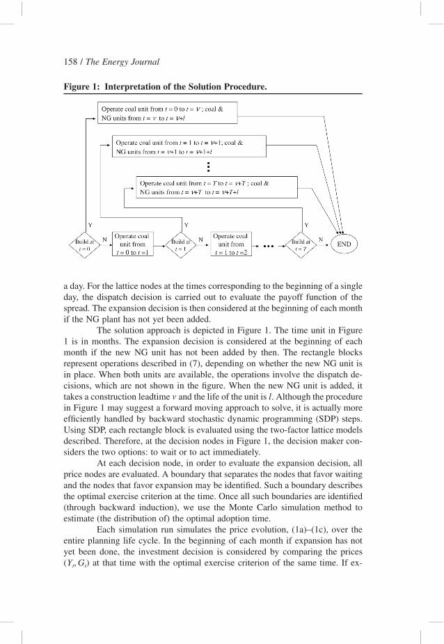
Figure 1: Interpretation of the Solution Procedure.
a day. For the lattice nodes at the times corresponding to the beginning of a singleday, the dispatch decision is carried out to evaluate the payoff function of thespread. The expansion decision is then considered at the beginning of each monthif the NG plant has not yet been added.
The solution approach is depicted in Figure 1. The time unit in Figure1 is in months. The expansion decision is considered at the beginning of eachmonth if the new NG unit has not been added by then. The rectangle blocksrepresent operations described in (7), depending on whether the new NG unit isin place. When both units are available, the operations involve the dispatch de-cisions, which are not shown in the figure. When the new NG unit is added, ittakes a construction leadtime and the life of the unit is . Although the procedurem lin Figure 1 may suggest a forward moving approach to solve, it is actually moreefficiently handled by backward stochastic dynamic programming (SDP) steps.Using SDP, each rectangle block is evaluated using the two-factor lattice modelsdescribed. Therefore, at the decision nodes in Figure 1, the decision maker con-siders the two options: to wait or to act immediately.
At each decision node, in order to evaluate the expansion decision, allprice nodes are evaluated. A boundary that separates the nodes that favor waitingand the nodes that favor expansion may be identified. Such a boundary describesthe optimal exercise criterion at the time. Once all such boundaries are identified(through backward induction), we use the Monte Carlo simulation method toestimate (the distribution of) the optimal adoption time.
Each simulation run simulates the price evolution, (1a)–(1c), over theentire planning life cycle. In the beginning of each month if expansion has notyet been done, the investment decision is considered by comparing the prices
at that time with the optimal exercise criterion of the same time. If ex-(Y , G )t t
Inducing Clean Technology in the Electricity Sector / 159
pansion is more profitable than waiting, the NG plant would be built and thisadoption time is recorded. The same simulation run then continues to simulatethe construction period , followed by the operational period of the new NGm lplant, and finally stops at the end of the life of the new NG plant. The profitassociated with this investment over its life cycle can be evaluated. Such a processis repeated for runs, with adoption times recorded, along with investmentN N Nprofits. The expected values of the optimal adoption time and the correspondinginvestment profit can be determined.
3. CASE STUDY
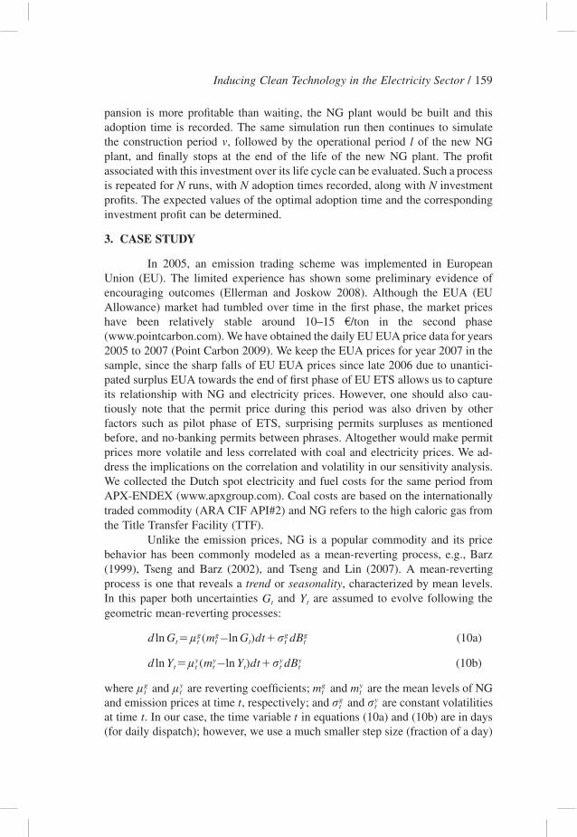
In 2005, an emission trading scheme was implemented in EuropeanUnion (EU). The limited experience has shown some preliminary evidence ofencouraging outcomes (Ellerman and Joskow 2008). Although the EUA (EUAllowance) market had tumbled over time in the first phase, the market priceshave been relatively stable around 10–15 €/ton in the second phase(www.pointcarbon.com). We have obtained the daily EU EUA price data for years2005 to 2007 (Point Carbon 2009). We keep the EUA prices for year 2007 in thesample, since the sharp falls of EU EUA prices since late 2006 due to unantici-pated surplus EUA towards the end of first phase of EU ETS allows us to captureits relationship with NG and electricity prices. However, one should also cau-tiously note that the permit price during this period was also driven by otherfactors such as pilot phase of ETS, surprising permits surpluses as mentionedbefore, and no-banking permits between phrases. Altogether would make permitprices more volatile and less correlated with coal and electricity prices. We ad-dress the implications on the correlation and volatility in our sensitivity analysis.We collected the Dutch spot electricity and fuel costs for the same period fromAPX-ENDEX (www.apxgroup.com). Coal costs are based on the internationallytraded commodity (ARA CIF API#2) and NG refers to the high caloric gas fromthe Title Transfer Facility (TTF).
Unlike the emission prices, NG is a popular commodity and its pricebehavior has been commonly modeled as a mean-reverting process, e.g., Barz(1999), Tseng and Barz (2002), and Tseng and Lin (2007). A mean-revertingprocess is one that reveals a trend or seasonality, characterized by mean levels.In this paper both uncertainties and are assumed to evolve following theG Yt t
geometric mean-reverting processes:
g g g gd ln G �l (m –ln G )dt�r dB (10a)t t t t t t
y y y yd ln Y �l (m –ln Y )dt�r dB (10b)t t t t t t
where and are reverting coefficients; and are the mean levels of NGg y g yl l m mt t t t
and emission prices at time , respectively; and and are constant volatilitiesg yt r rt t
at time . In our case, the time variable in equations (10a) and (10b) are in dayst t(for daily dispatch); however, we use a much smaller step size (fraction of a day)
160 / The Energy Journal
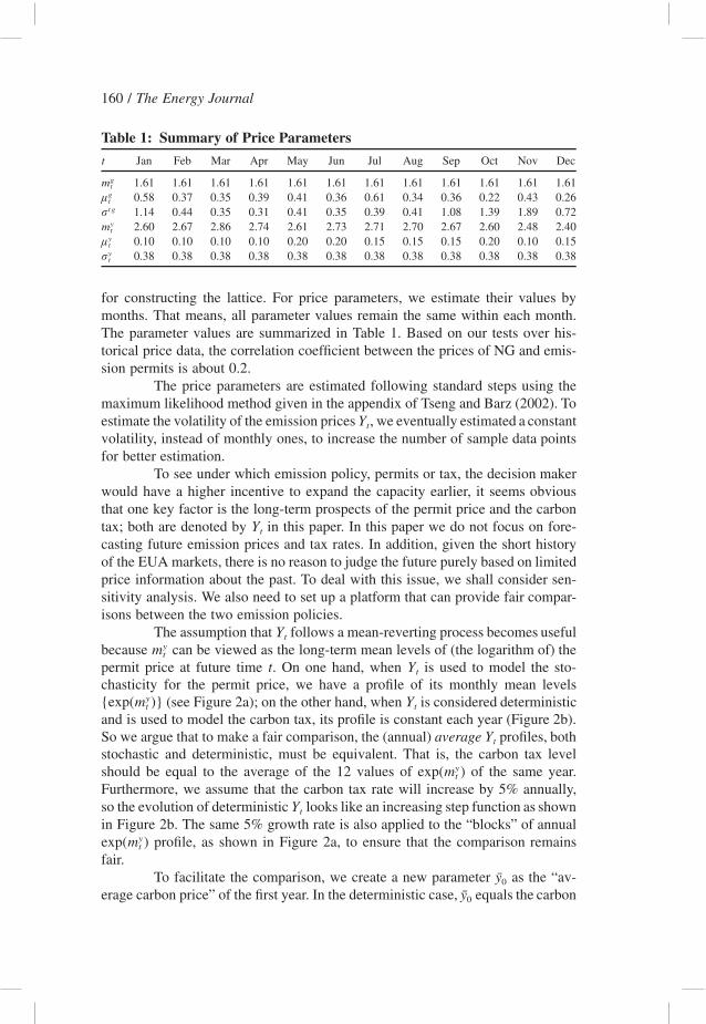
Table 1: Summary of Price Parameters
t Jan Feb Mar Apr May Jun Jul Aug Sep Oct Nov Dec
gmt 1.61 1.61 1.61 1.61 1.61 1.61 1.61 1.61 1.61 1.61 1.61 1.61glt 0.58 0.37 0.35 0.39 0.41 0.36 0.61 0.34 0.36 0.22 0.43 0.26t gr 1.14 0.44 0.35 0.31 0.41 0.35 0.39 0.41 1.08 1.39 1.89 0.72ymt 2.60 2.67 2.86 2.74 2.61 2.73 2.71 2.70 2.67 2.60 2.48 2.40
ylt 0.10 0.10 0.10 0.10 0.20 0.20 0.15 0.15 0.15 0.20 0.10 0.15yrt 0.38 0.38 0.38 0.38 0.38 0.38 0.38 0.38 0.38 0.38 0.38 0.38
for constructing the lattice. For price parameters, we estimate their values bymonths. That means, all parameter values remain the same within each month.The parameter values are summarized in Table 1. Based on our tests over his-torical price data, the correlation coefficient between the prices of NG and emis-sion permits is about 0.2.
The price parameters are estimated following standard steps using themaximum likelihood method given in the appendix of Tseng and Barz (2002). Toestimate the volatility of the emission prices , we eventually estimated a constantYt
volatility, instead of monthly ones, to increase the number of sample data pointsfor better estimation.
To see under which emission policy, permits or tax, the decision makerwould have a higher incentive to expand the capacity earlier, it seems obviousthat one key factor is the long-term prospects of the permit price and the carbontax; both are denoted by in this paper. In this paper we do not focus on fore-Yt
casting future emission prices and tax rates. In addition, given the short historyof the EUA markets, there is no reason to judge the future purely based on limitedprice information about the past. To deal with this issue, we shall consider sen-sitivity analysis. We also need to set up a platform that can provide fair compar-isons between the two emission policies.
The assumption that follows a mean-reverting process becomes usefulYt
because can be viewed as the long-term mean levels of (the logarithm of) theymt
permit price at future time . On one hand, when is used to model the sto-t Yt
chasticity for the permit price, we have a profile of its monthly mean levels(see Figure 2a); on the other hand, when is considered deterministicy{exp(m )} Yt t
and is used to model the carbon tax, its profile is constant each year (Figure 2b).So we argue that to make a fair comparison, the (annual) average profiles, bothYt
stochastic and deterministic, must be equivalent. That is, the carbon tax levelshould be equal to the average of the 12 values of of the same year.yexp(m )t
Furthermore, we assume that the carbon tax rate will increase by 5% annually,so the evolution of deterministic looks like an increasing step function as shownYt
in Figure 2b. The same 5% growth rate is also applied to the “blocks” of annualprofile, as shown in Figure 2a, to ensure that the comparison remainsyexp(m )t
fair.To facilitate the comparison, we create a new parameter as the “av-y0
erage carbon price” of the first year. In the deterministic case, equals the carbony0
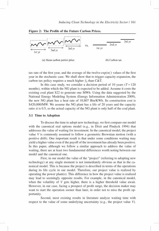
Inducing Clean Technology in the Electricity Sector / 161
Figure 2: The Profile of the Future Carbon Prices.
tax rate of the first year, and the average of the twelve values of the firstyexp(m )t
year in the stochastic case. We shall show that to trigger capacity expansion, thecarbon tax policy requires a much higher than C&T.y0
In this case study, we consider a decision period of 10 years (T�120months), within which the NG plant is expected to be added. Assume it costs theexisting coal plant $22 to generate one MWh. Using the data suggested by theNational Energy Modeling System (Energy Information Administration 2009),the new NG plant has a heat rate of 10,807 Btu/KWh. Its construction cost is$420,000/MW. We assume the NG plant has a life of 20 years and the capacityratio is 0.5, so the actual capacity of the NG plant is only half of the coal plant.�
3.1 Time to Adoption
To discuss the time to adopt new technology, we first compare our modelwith the canonical real options model (e.g., in Dixit and Pindyck 1994) thataddresses the value of waiting for investment. In the canonical model, the projectvalue is commonly assumed to follow a geometric Brownian motion (with aVpositive drift). One important result is that under some conditions waiting mayyield a higher value even if the payoff of the investment has already been positive.In this paper, although we follow a similar approach to address the value ofwaiting, there are at least two fundamental differences worth noting between ourmodel and the canonical one.
First, in our model the value of the “project” (referring to adopting newtechnology) at any single moment is not immediately obvious as that in the ca-nonical model. This is because the project is described in terms of the operationsduring its life cycle in our model. Therefore, our project value is realized byoperating the power plant(s). This difference in how the project value is realizedmay lead to seemingly opposite results. For example, in the canonical model,when the volatility of gets higher, there is a higher threshold value await.VHowever, in our case, facing a prospect of profit surge, the decision maker maywant to start the operation sooner than later, in order not to miss the profit op-portunity.
Second, most existing results in literature analyze waiting time withrespect to the value of some underlying uncertainty (e.g., the project value ).V
162 / The Energy Journal
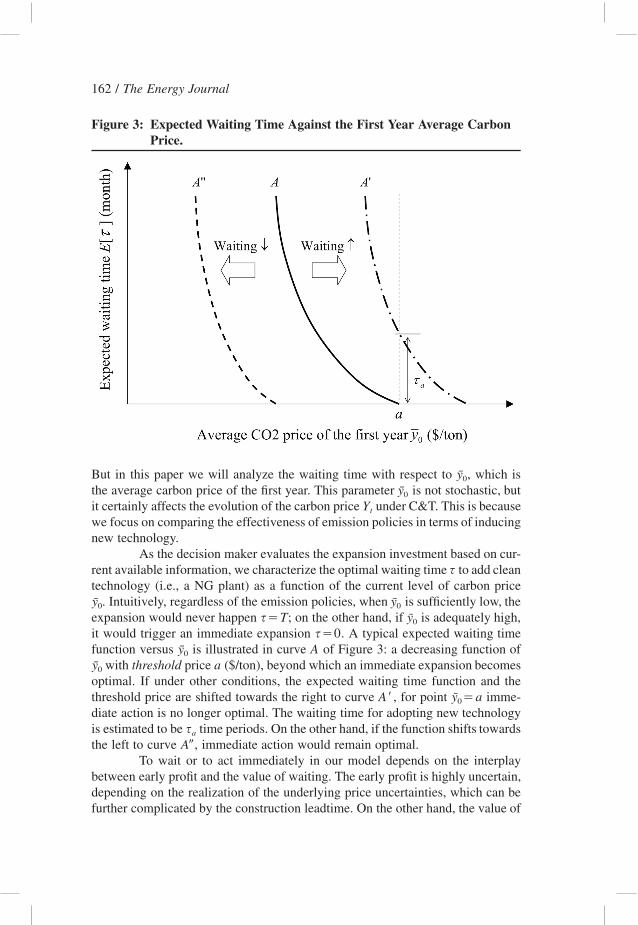
Figure 3: Expected Waiting Time Against the First Year Average CarbonPrice.
But in this paper we will analyze the waiting time with respect to , which isy0
the average carbon price of the first year. This parameter is not stochastic, buty0
it certainly affects the evolution of the carbon price under C&T. This is becauseYt
we focus on comparing the effectiveness of emission policies in terms of inducingnew technology.
As the decision maker evaluates the expansion investment based on cur-rent available information, we characterize the optimal waiting time to add cleanstechnology (i.e., a NG plant) as a function of the current level of carbon price
. Intuitively, regardless of the emission policies, when is sufficiently low, they y0 0
expansion would never happen ; on the other hand, if is adequately high,s�T y0
it would trigger an immediate expansion . A typical expected waiting times�0function versus is illustrated in curve of Figure 3: a decreasing function ofy A0
with threshold price ($/ton), beyond which an immediate expansion becomesy a0
optimal. If under other conditions, the expected waiting time function and thethreshold price are shifted towards the right to curve , for point imme-A� y �a0
diate action is no longer optimal. The waiting time for adopting new technologyis estimated to be time periods. On the other hand, if the function shifts towardssa
the left to curve , immediate action would remain optimal.A�To wait or to act immediately in our model depends on the interplay
between early profit and the value of waiting. The early profit is highly uncertain,depending on the realization of the underlying price uncertainties, which can befurther complicated by the construction leadtime. On the other hand, the value of
Inducing Clean Technology in the Electricity Sector / 163
Table 2: Comparison of Threshold Prices of Both Emission Policies
C&T Tax
($/ton)y0 (m)E[s] Profit ($)J ($/ton)y0 (m)E[s] Profit ($)J
30.3 120.0 0.0 79.3 120.0 0.030.4 112.2 17.6 79.4 120.0 0.030.5 99.7 49.1 79.5† 0.0 0.030.6 71.1 107.9 79.6 0.0 947.530.7 9.5 641.930.8† 0.0 1636.0
†: threshold price
waiting includes interest saving from deferring the payment and the typical optionvalue of waiting. Both are uncertain. To simplify the matter, we first assume thatthe construction of the new NG plant can be done instantaneously (i.e., ).m�0(The impact of a non-zero construction time will be analyzed later.) We thenfocus on analyzing the threshold prices under both emission policies. The resultsconcerning the threshold prices are summarized in Table 2. The threshold pricesfor the C&T permit and tax are $30.8 and $79.5, respectively. This suggests thatit requires a much higher level of tax ( $80) than permit prices ( $31) toy � y �0 0
induce capacity expansion.Table 2 implies that for C&T when the first year carbon price is abovey0
$30.3 but less than $30.8, the investment yields a positive but non-optimal ex-pected profit. The average waiting times are estimated using the Monte Carlosimulation. When is very close to $30.8, almost all simulation instances rec-y0
ommend immediate action; on the other hand, when is close to $30.3, mosty0
simulation instances recommend doing nothing, i.e., setting months.s�T�120For tax policy, it turns out that the threshold price is the same as the break-evenprice, where zero net profit is achieved. This issue will be discussed in greaterdetail later.
Table 2 also indicates that when increases, the expected waiting timey0
decreases very quickly to 0 (from 120 months down to 0 within 50 cents)E[s]for the permit case. When the tax policy is considered, the behavior of versusE[s]
is similar to that of the permit case except that the curve decreases abruptly,y0
resembling a step function. To explain the steepness of the function under C&T,note the definition of , which is the mean carbon price of the first year. They0
mean carbon prices in subsequent years are compounded annually with a fixedrate. So a 50-cent difference in has a significant profit impact in this operationy0
that only generates 1MW of power.To explain the sudden drop of the expected waiting time function under
tax policy, we need to revisit the payoff function in equation (9). As mentionedpreviously in Section 2.3, under tax policy the decision maker faces a fixed rev-enue stream and a cost uncertainty , with the growth rate of the(0.5Y �C) Gt t
revenue less than the discount rate. Without considering the cost uncertainty ,Gt
164 / The Energy Journal
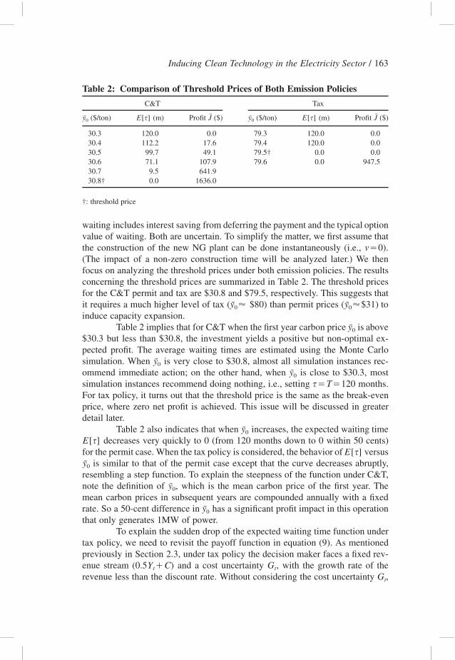
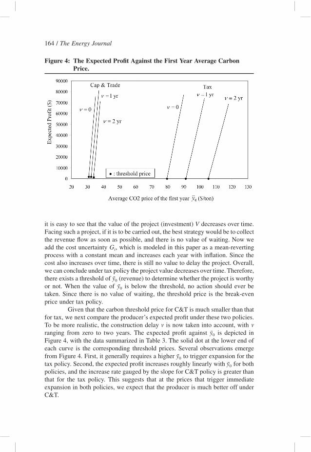
Figure 4: The Expected Profit Against the First Year Average CarbonPrice.
it is easy to see that the value of the project (investment) decreases over time.VFacing such a project, if it is to be carried out, the best strategy would be to collectthe revenue flow as soon as possible, and there is no value of waiting. Now weadd the cost uncertainty , which is modeled in this paper as a mean-revertingGt
process with a constant mean and increases each year with inflation. Since thecost also increases over time, there is still no value to delay the project. Overall,we can conclude under tax policy the project value decreases over time. Therefore,there exists a threshold of (revenue) to determine whether the project is worthyy0
or not. When the value of is below the threshold, no action should ever bey0
taken. Since there is no value of waiting, the threshold price is the break-evenprice under tax policy.
Given that the carbon threshold price for C&T is much smaller than thatfor tax, we next compare the producer’s expected profit under these two policies.To be more realistic, the construction delay is now taken into account, withm mranging from zero to two years. The expected profit against is depicted iny0
Figure 4, with the data summarized in Table 3. The solid dot at the lower end ofeach curve is the corresponding threshold prices. Several observations emergefrom Figure 4. First, it generally requires a higher to trigger expansion for they0
tax policy. Second, the expected profit increases roughly linearly with for bothy0
policies, and the increase rate gauged by the slope for C&T policy is greater thanthat for the tax policy. This suggests that at the prices that trigger immediateexpansion in both policies, we expect that the producer is much better off underC&T.
Inducing Clean Technology in the Electricity Sector / 165
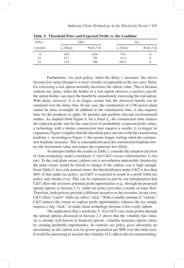
Table 3: Threshold Price and Expected Profit vs. the Leadtime
Policy C&T Tax
(month)m ($/ton)y0 Profit ($)J ($/ton)y0 Profit ($)J
0 30.8 1636 79.5 012 32.3 793 91.4 024 33.8 468 105.4 0
Furthermore, for each policy, when the delay increases, the curvesmbecome less steep (though it is more visually recognizable in the tax case). Delayfor exercising a real option normally decreases the option value. This is becausewithout any delay, when the holder of a real option observes a positive payoff,the option holder can enjoy the benefit by immediately exercising the real option.With delay, however, it is no longer certain that the observed benefit can besustained over the delay time. In our case, the construction of a NG power plantcannot be done overnight. In addition to the construction time, it also requirestime for the producer to apply for permits and perform relevant environmentalstudies. As implied from Figure 4, for a fixed , the construction time reducesy0
the expected profit; and for the same level of profitability (expected profit value),a technology with a shorter construction time requires a smaller to trigger itsy0
expansion. Figure 4 implies that the threshold price elevates with the constructionleadtime . According to Figure 3, this means longer waiting when the construc-mtion leadtime increases. This is reasonable because the construction leadtime low-ers the investment value and makes the expansion less likely.
To interpret further the results in Table 2, consider the adoption decisionof clean technology under a stochastic (for C&T) versus a deterministic (forY Yt t
tax). To the coal plant owner, carbon cost is nevertheless undesirable. Intuitively,the plant owner would be forced to change if the carbon cost is high enough.From Table 2, for a risk neutral owner, the threshold price under C&T is less than40% of that under tax policy, yet C&T is expected to result in a profit while taxpolicy only breaks even. This can be explained in part by our interpretation thatC&T offers the investors potential profit opportunities (e.g., through the proposedspread options in Section 2.3), while tax policy provides a steady revenue flow.Therefore, both policies provide a different incentive to the investors. In our view,C&T offers “carrot” while tax offers “stick.” With a smaller amount of “carrots,”C&T induces the owner to explore profit opportunities; whereas the tax simplyimposes a big “stick,” to make clean technology become a less costly option.
The implication that a stochastic (for C&T) can create profits throughYt
the spread options discussed in Section 2.3 shows that the volatility has value.As is already well known in financial options, volatility increases option valuesby creating profitable opportunities. In contrast, tax policy gives absolutely nouncertainty on the carbon cost for power generation per MW over the entire year.It would be interesting to see how the volatility of affects the investment timing.Yt
166 / The Energy Journal
In the next section we shall show that higher volatility makes C&T more attractiveand reduces the waiting time.
While tax could be preferred by risk-averse producers or plant owners,who generally dislike market uncertainties created by C&T, our study shows thatfor the tax policy to be as effective as C&T (in terms of inducing clean technol-ogy), the tax level must be very high, and as a result, producers and plant ownersare actually better off under C&T (see Figure 4). Thus far we have consideredthe decision maker to be risk neutral. What if the decision maker is risk-averse?Would risk aversion make the tax policy more appealing? It turns out that withrisk aversion the plant owners are even much better off under C&T. This will bedemonstrated in a later section.
3.2 Sensitivity Analysis
With the limited experience we have so far about the Regional Green-house Gas Initiative in the US, the future permit price and relationship withelectricity prices remains unknown even if the offset provision is in place tocontain permit prices. In this paper, we have estimated the parameters based onthe historical data of the Dutch electricity, fuel, and EU permits markets. It maybe more insightful to interpret our result from the comparative perspective byperforming sensitivity analyses on key parameters. The two parameters for whichwe will change values are the volatility of permit price ( ) and the correlationyrt
between the prices of NG and the permit.
Changing volatility yrt
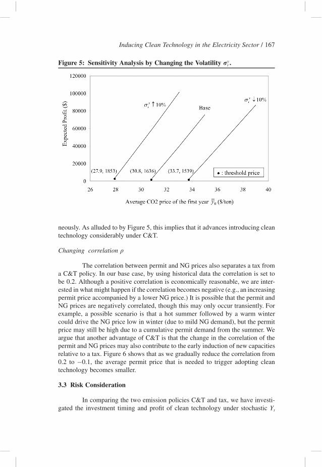
As we have argued, the volatility is the main factor that C&T yieldsmore expected profit than tax to the plant owner. In Figure 5, we show the extentthat the expected profit would change if the value of the volatility for the permitprice given in Table 1 is increased (or decreased) by 10%. Figure 5 suggests thatwhen the volatility increases (decreases), the relationship of the expected profitshifts almost parallel to the left (right) from original curves, indicating a smallerpermit price is required to trigger a capacity expansion under a greater volatility.As seen, roughly a 10% increase in volatility lowers the trigger price by threedollars. The result also shows that even if the volatility that we use in this casestudy is underestimated, the C&T policy is still likely to be more effective thanthe tax policy in terms of inducing capacity expansion.
This result has another implication. As a large fraction of coal producersfacing the carbon regulation would adopt clean technologies simultaneously (e.g.,NG plant), it would effectively increase the demand of NG and suppress thedemand for coal and CO2 permits. In the extreme, if NG plants always stay atmarginal, and CO2 costs are fully passed through, the electricity prices will beclosely related to NG and permit prices. The volatilities would likely escalate asthe demand of NG from these producers move in the same direction simulta-
Inducing Clean Technology in the Electricity Sector / 167
Figure 5: Sensitivity Analysis by Changing the Volatility .yrt
neously. As alluded to by Figure 5, this implies that it advances introducing cleantechnology considerably under C&T.
Changing correlation q
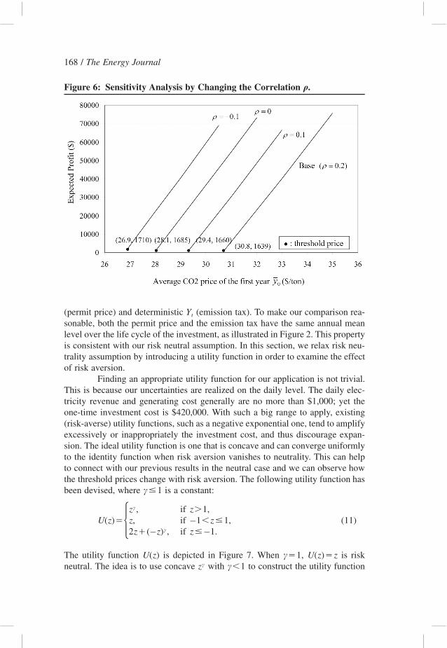
The correlation between permit and NG prices also separates a tax froma C&T policy. In our base case, by using historical data the correlation is set tobe 0.2. Although a positive correlation is economically reasonable, we are inter-ested in what might happen if the correlation becomes negative (e.g., an increasingpermit price accompanied by a lower NG price.) It is possible that the permit andNG prices are negatively correlated, though this may only occur transiently. Forexample, a possible scenario is that a hot summer followed by a warm wintercould drive the NG price low in winter (due to mild NG demand), but the permitprice may still be high due to a cumulative permit demand from the summer. Weargue that another advantage of C&T is that the change in the correlation of thepermit and NG prices may also contribute to the early induction of new capacitiesrelative to a tax. Figure 6 shows that as we gradually reduce the correlation from0.2 to –0.1, the average permit price that is needed to trigger adopting cleantechnology becomes smaller.
3.3 Risk Consideration
In comparing the two emission policies C&T and tax, we have investi-gated the investment timing and profit of clean technology under stochastic Yt
168 / The Energy Journal
Figure 6: Sensitivity Analysis by Changing the Correlation .q
(permit price) and deterministic (emission tax). To make our comparison rea-Yt
sonable, both the permit price and the emission tax have the same annual meanlevel over the life cycle of the investment, as illustrated in Figure 2. This propertyis consistent with our risk neutral assumption. In this section, we relax risk neu-trality assumption by introducing a utility function in order to examine the effectof risk aversion.
Finding an appropriate utility function for our application is not trivial.This is because our uncertainties are realized on the daily level. The daily elec-tricity revenue and generating cost generally are no more than $1,000; yet theone-time investment cost is $420,000. With such a big range to apply, existing(risk-averse) utility functions, such as a negative exponential one, tend to amplifyexcessively or inappropriately the investment cost, and thus discourage expan-sion. The ideal utility function is one that is concave and can converge uniformlyto the identity function when risk aversion vanishes to neutrality. This can helpto connect with our previous results in the neutral case and we can observe howthe threshold prices change with risk aversion. The following utility function hasbeen devised, where is a constant:c�1
cz , if z�1,U(z)� z, if –1�z�1, (11)� c2z�(–z) , if z� –1.
The utility function is depicted in Figure 7. When , is riskU(z) c�1 U(z)�zneutral. The idea is to use concave with to construct the utility functioncz c�1
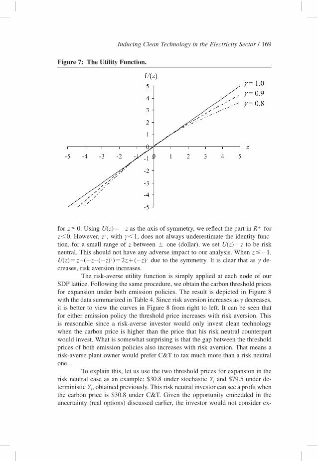
Inducing Clean Technology in the Electricity Sector / 169
Figure 7: The Utility Function.
for . Using as the axis of symmetry, we reflect the part in for�z�0 U(z)�–z R. However, , with , does not always underestimate the identity func-cz�0 z c�1
tion, for a small range of between one (dollar), we set to be riskz � U(z)�zneutral. This should not have any adverse impact to our analysis. When ,z� –1
due to the symmetry. It is clear that as de-c cU(z)�z–(–z–(–z) )�2z�(–z) ccreases, risk aversion increases.
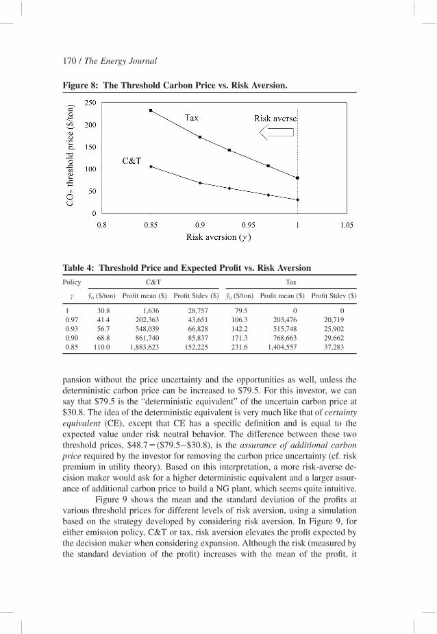
The risk-averse utility function is simply applied at each node of ourSDP lattice. Following the same procedure, we obtain the carbon threshold pricesfor expansion under both emission policies. The result is depicted in Figure 8with the data summarized in Table 4. Since risk aversion increases as decreases,cit is better to view the curves in Figure 8 from right to left. It can be seen thatfor either emission policy the threshold price increases with risk aversion. Thisis reasonable since a risk-averse investor would only invest clean technologywhen the carbon price is higher than the price that his risk neutral counterpartwould invest. What is somewhat surprising is that the gap between the thresholdprices of both emission policies also increases with risk aversion. That means arisk-averse plant owner would prefer C&T to tax much more than a risk neutralone.
To explain this, let us use the two threshold prices for expansion in therisk neutral case as an example: $30.8 under stochastic and $79.5 under de-Yt
terministic , obtained previously. This risk neutral investor can see a profit whenYt
the carbon price is $30.8 under C&T. Given the opportunity embedded in theuncertainty (real options) discussed earlier, the investor would not consider ex-
170 / The Energy Journal
Figure 8: The Threshold Carbon Price vs. Risk Aversion.
Table 4: Threshold Price and Expected Profit vs. Risk Aversion
Policy C&T Tax
c ($/ton)y0 Profit mean ($) Profit Stdev ($) ($/ton)y0 Profit mean ($) Profit Stdev ($)
1 30.8 1,636 28,757 79.5 0 00.97 41.4 202,363 43,651 106.3 203,476 20,7190.93 56.7 548,039 66,828 142.2 515,748 25,9020.90 68.8 861,740 85,837 171.3 768,663 29,6620.85 110.0 1,883,623 152,225 231.6 1,404,557 37,283
pansion without the price uncertainty and the opportunities as well, unless thedeterministic carbon price can be increased to $79.5. For this investor, we cansay that $79.5 is the “deterministic equivalent” of the uncertain carbon price at$30.8. The idea of the deterministic equivalent is very much like that of certaintyequivalent (CE), except that CE has a specific definition and is equal to theexpected value under risk neutral behavior. The difference between these twothreshold prices, $48.7�($79.5–$30.8), is the assurance of additional carbonprice required by the investor for removing the carbon price uncertainty (cf. riskpremium in utility theory). Based on this interpretation, a more risk-averse de-cision maker would ask for a higher deterministic equivalent and a larger assur-ance of additional carbon price to build a NG plant, which seems quite intuitive.
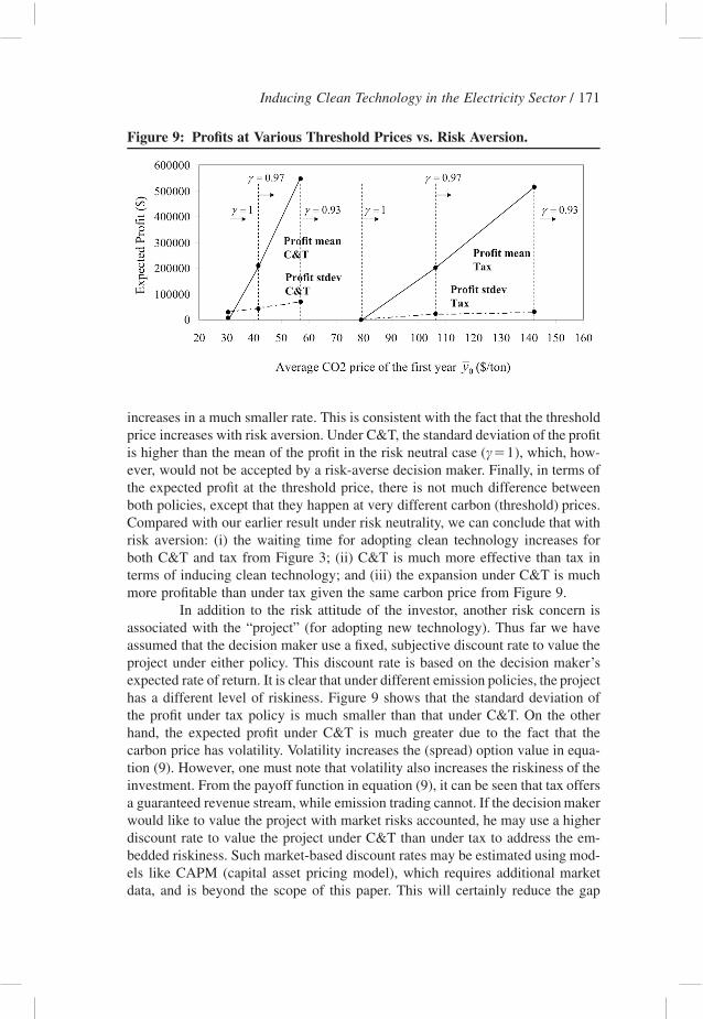
Figure 9 shows the mean and the standard deviation of the profits atvarious threshold prices for different levels of risk aversion, using a simulationbased on the strategy developed by considering risk aversion. In Figure 9, foreither emission policy, C&T or tax, risk aversion elevates the profit expected bythe decision maker when considering expansion. Although the risk (measured bythe standard deviation of the profit) increases with the mean of the profit, it
Inducing Clean Technology in the Electricity Sector / 171
Figure 9: Profits at Various Threshold Prices vs. Risk Aversion.
increases in a much smaller rate. This is consistent with the fact that the thresholdprice increases with risk aversion. Under C&T, the standard deviation of the profitis higher than the mean of the profit in the risk neutral case ( ), which, how-c�1ever, would not be accepted by a risk-averse decision maker. Finally, in terms ofthe expected profit at the threshold price, there is not much difference betweenboth policies, except that they happen at very different carbon (threshold) prices.Compared with our earlier result under risk neutrality, we can conclude that withrisk aversion: (i) the waiting time for adopting clean technology increases forboth C&T and tax from Figure 3; (ii) C&T is much more effective than tax interms of inducing clean technology; and (iii) the expansion under C&T is muchmore profitable than under tax given the same carbon price from Figure 9.
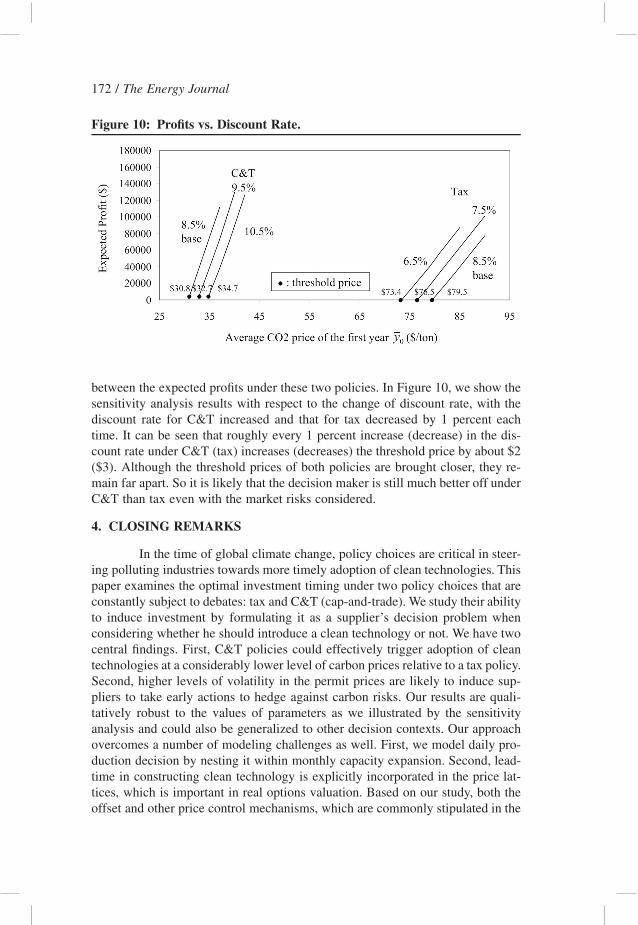
In addition to the risk attitude of the investor, another risk concern isassociated with the “project” (for adopting new technology). Thus far we haveassumed that the decision maker use a fixed, subjective discount rate to value theproject under either policy. This discount rate is based on the decision maker’sexpected rate of return. It is clear that under different emission policies, the projecthas a different level of riskiness. Figure 9 shows that the standard deviation ofthe profit under tax policy is much smaller than that under C&T. On the otherhand, the expected profit under C&T is much greater due to the fact that thecarbon price has volatility. Volatility increases the (spread) option value in equa-tion (9). However, one must note that volatility also increases the riskiness of theinvestment. From the payoff function in equation (9), it can be seen that tax offersa guaranteed revenue stream, while emission trading cannot. If the decision makerwould like to value the project with market risks accounted, he may use a higherdiscount rate to value the project under C&T than under tax to address the em-bedded riskiness. Such market-based discount rates may be estimated using mod-els like CAPM (capital asset pricing model), which requires additional marketdata, and is beyond the scope of this paper. This will certainly reduce the gap
172 / The Energy Journal
Figure 10: Profits vs. Discount Rate.
between the expected profits under these two policies. In Figure 10, we show thesensitivity analysis results with respect to the change of discount rate, with thediscount rate for C&T increased and that for tax decreased by 1 percent eachtime. It can be seen that roughly every 1 percent increase (decrease) in the dis-count rate under C&T (tax) increases (decreases) the threshold price by about $2($3). Although the threshold prices of both policies are brought closer, they re-main far apart. So it is likely that the decision maker is still much better off underC&T than tax even with the market risks considered.
4. CLOSING REMARKS
In the time of global climate change, policy choices are critical in steer-ing polluting industries towards more timely adoption of clean technologies. Thispaper examines the optimal investment timing under two policy choices that areconstantly subject to debates: tax and C&T (cap-and-trade). We study their abilityto induce investment by formulating it as a supplier’s decision problem whenconsidering whether he should introduce a clean technology or not. We have twocentral findings. First, C&T policies could effectively trigger adoption of cleantechnologies at a considerably lower level of carbon prices relative to a tax policy.Second, higher levels of volatility in the permit prices are likely to induce sup-pliers to take early actions to hedge against carbon risks. Our results are quali-tatively robust to the values of parameters as we illustrated by the sensitivityanalysis and could also be generalized to other decision contexts. Our approachovercomes a number of modeling challenges as well. First, we model daily pro-duction decision by nesting it within monthly capacity expansion. Second, lead-time in constructing clean technology is explicitly incorporated in the price lat-tices, which is important in real options valuation. Based on our study, both theoffset and other price control mechanisms, which are commonly stipulated in the
Inducing Clean Technology in the Electricity Sector / 173
proposed and the existing climate policies with an attempt to reduce permit pricesor suppress price volatility, may delay clean technology investments. This sug-gests that if leveling the playground of these highly affected industries is the mainpurpose, a lump-sum rebate from permits auctions’ revenues might be a betterchoice without postponing clean technology adoptions.
ACKNOWLEDGMENT
The authors would like to thank Afzal Siddiqui, three anonymous ref-erees and the editor for many helpful comments. The first author is partiallysupported by a grant from the Graduate Research Council (GRC) of Universityof California, Merced.
REFERENCES
Barz, G. (1999). “Stochastic Financial Models for Electricity Derivatives.” Ph.D. Dissertation, Stan-ford University.
Carmona, R. and V. Durrleman (2003). “Pricing and Hedging Spread Options.” SIAM Review 45(4):627–685.
Chen, Y., J. Sijm, B. F. Hobbs and W. Lise (2008). “Implications of CO2 Emissions Trading for Short-run Electricity Market Outcomes in Northwest Europe.” Journal of Regulatory Economics 34: 251–281.
Coria, J. (2009). “Taxes, Permits, and the Diffusion of a New Technology.” Resources and EnergyEconomics 31: 249–271.
Dixit, A. K. and R. S. Pindyck (1994). Investment under Uncertainty. Princeton.Ellerman, D. and P. Joskow (2008). “The European Union’s Emissions Trading System in Perspec-
tive.” Report prepared for the Pew Center on Global Climate Change, http://www.pewclimate.org/docUploads/EU-ETS-In-Perspective-Report.pdf.
Energy Information Administration (2009). “Assumptions to National Energy Modeling System2009.”http://www.eia.doe.gov/oiaf/aeo/assumption/pdf/0554(2009).pdf
Green, R. (2008). “Carbon Tax and Carbon Permits: The Impact on Generators’ Risks.” The EnergyJournal 29(3): 67–90.
Intergovernmental Panel on Climate Change (2007). “Climate Change 2007: Synthesis Report.”Jaffe, A. B., R. G. Newell and R. N. Stavins (2002). “Environmental Policy and Technology Change.”
Environmental and Resource Economics 22: 41–69.Kennedy, P. W. and B. Lapiante (1999). “Environmental Policy and Time Consistency: Emission
Taxes and Emission Trading.” In: Petrakis, E., Sartzetakis, E.S., Xepapadeas, A. eds., Environ-mental Regulation and Market Power: Competition, Time Consistency, and International Trade:Edward Elgar, Cheltenham Glos, UK, pp. 116–144.
Mansur, E. (2007). “Prices vs. Quantities: Environmental Regulation and Imperfect Competition.”NBER Working Paper No. 13510.
Milliman, S. R. and R. Price (1989). “Firms’ Incentives to Promote Technological Change in PollutionControl.” Journal of Environmental Economics and Management 17: 247–265.
Montero, J. P. (2002a). “Market Structure and Environmental Innovation.” Journal of Applied Eco-nomics 5(2): 293–325.
Montero, J. P. (2002b). “Permits Standards, and Technology Innovation.” Journal of EnvironmentalEconomics and Management 44: 23–44.
Parry, I. W. H., L. H. Goulder and D. Burtraw (1997). “Revenue-Raising vs. Other Approaches toEnvironmental Protection: The Critical Significance of Existing Tax Distortion.” Rand Journal ofEconomics 28(4): 708–731.
174 / The Energy Journal
Point Carbon (2009). “PointCarbon: Provide Critical Insights into Energy and Environmental Mar-kets.” http://www.pointcarbon.com.
Requate, T. and W. Unold (2003). “Environmental Policy Incentives to Adopt Advanced AbatementTechnology: Will the True Ranking Please Stand Up?” European Economic Review 47(1): 125–146.
Stavins, R. N. (1995). “Transaction Costs and Tradable Permits.” Journal of Environmental Economicsand Management 29: 133–147.
Sijm, J, K. Neuhoff and Y. Chen (2006). “CO2 Cost Pass-through and Windfall Profits in the PowerSector.” Climate Policy 6: 49–72.
Tseng, C. L. and G. Barz (2002). “Short-term Generation Asset Valuation: a Real Options Approach.”Operations Research 50(2):297–310.
Tseng, C. L. and K. Y. Lin (2007). “A Framework using Two-factor Price Lattices for GenerationAsset Valuation.” Operations Research 55(2):127–153.
Weitzman, M. (1974). “Prices vs. Quantities.” The Review of Economics Studies 41(4): 477–491.