Wireless NetworksDOI 10.1007/s11276-006-5064-1

Indoor location tracking using RSSI readings from a single Wi-Fiaccess pointG. V. Zaruba · M. Huber · F. A. Kamangar ·I. Chlamtac

Published online: 8 June 2006C© Springer Science + Business Media, LLC 2006

Abstract This paper describes research towards a systemfor locating wireless nodes in a home environment requiringmerely a single access point. The only sensor reading used forthe location estimation is the received signal strength indica-tion (RSSI) as given by an RF interface, e.g., Wi-Fi. Wirelesssignal strength maps for the positioning filter are obtained bya two-step parametric and measurement driven ray-tracingapproach to account for absorption and reflection charac-teristics of various obstacles. Location estimates are thencomputed using Bayesian filtering on sample sets derivedby Monte Carlo sampling. We outline the research leadingto the system and provide location performance metrics us-ing trace-driven simulations and real-life experiments. Ourresults and real-life walk-troughs indicate that RSSI read-ings from a single access point in an indoor environmentare sufficient to derive good location estimates of users withsub-room precision.

Keywords Location estimation . System design . Wirelessexperiments . Simulation . Monte Carlo sampling

G. V. Zaruba (�) · M. Huber · F. A. KamangarDepartment of Computer Science and Engineering,The University of Texas at Arlingtone-mail: zaruba@cse.uta.edu

M. Hubere-mail: huber@cse.uta.edu

F. A. Kamangare-mail: kamangar@cse.uta.edu

I. ChlamtacCreate-Net and University of Trento,email: chlamtac@create-net.it

1. Introduction and motivation

The globally pervasive computing environments [29] of thefuture with their large number of heterogeneous, mobilecomputing nodes pose many challenges but also offer un-precedented opportunities. In such environments, sensorsand other computational nodes are omnipresent while peo-ple may carry a large numbers of small, connected devicesthat permit communication and computation at any pointin time. However, to harvest the power of such comput-ing environments it is necessary that computing nodes arecontext-aware, i.e., that they are able to adjust their operationto the particular context in which they currently operate. Animportant part of context-awareness is location-awareness[3,13], where nodes are enabled to obtain estimates of theirphysical location, thus tailoring the physical environmentand its software representation to the user. Overall, in perva-sive computing the more information is available about thelocal environment of users and computing entities the betterthe applications can adapt to the user. Thus, we argue that es-timating location via various sensor readings is an importantenabler of pervasive computing.

Location aware computing has a bright future in the fieldsof personal navigation, personal security, prompt healthcareand entertainment. Furthermore, information on the physi-cal location of mobile nodes can greatly help in urban searchand rescue missions, as well as enable geographical routingin ad hoc multi-hop networks. The determination of physi-cal location is sometimes referred to as location estimation,location identification, localization, positioning or geoloca-tion identification. Recent projects and interest in intelligenthome environments such as [5] require the environment toknow the whereabouts of the inhabitants in order to adapt theenvironment to them. In this paper we restrict ourselves toindoor localization, more precisely to in-home localization

Springer

Wireless Networks

(without loosing the generality to apply our results to anyindoor environment).

Due to the fact that networked mobile users are enabledwith wireless radio communication network interfaces (suchas Wi-Fi), protocols that provide location estimation basedon the received signal strength indication (RSSI) of wirelessaccess points are becoming more-and-more popular, precise,and sophisticated. The main benefit of RSSI measurementbased systems is that they do not require any additionalsensor/actuator infrastructure but use already available com-munication parameters and downloadable wireless maps forthe position determination.

The work we are presenting relies only on received signalstrength measurements from wireless radio access pointsto determine the location of users. The major contributionof our paper is to show that good results can be achievedwith readings from a single access point. This is in contrastto previous works where at least three access points wererequired to localize users inside office buildings restricted tothe corridors of these buildings.

1.1. Localization techniques

The best-known location determination system is the GlobalPositioning System (GPS) [8]. A GPS receiver can estimateits location by measuring the propagation time of GHz rangeradio signals from several satellites to the receiver. Although,after the recent liberalization of GPS the precision of the ob-tained GPS position is quite accurate (down to a meter), GPSreceivers need to have line-of-sight to at least three or foursatellites in the sky. This restriction of GPS prohibits/restrictsits use in dense urban environments, indoors, and in areaswith tall and dense vegetation where line of sight to the re-quired number of satellites is not available. Moreover GPSlocalization is not reliable in a pervasive computing context,where small wearable and implanted terminals might be car-ried in a way that restricts line-of-sight to the GPS satellites.

Although GPS is the widest spread (and global) position-ing system, there are several other approaches available forlocation estimation and even more have been proposed inthe literature. The types of sensors used to obtain the lo-cation information vary from ultrasonic through photonicto radio signal strength measurement sensors. Most of theavailable and proposed location identification systems relyon proprietary and deployment-expensive infrastructure andprotocols. Wide area cellular systems use either mobile ter-minal integrated GPS receivers, or triangulate their posi-tion based on received signal strengths from several known-location base stations [18,25]. Since our work is focusedtowards the indoor environment we will not revisit outdoorpositioning systems. In the indoor environment, infraredand laser transmitter/receiver systems [1,28], ultrasonic sen-sor/actuator systems [21], computer vision systems [7,16],

physical contact [20] and close proximity radio identification(RFID) sensor [27] based localization systems have beenproposed and built to track mobile users. RSSI based loca-tion systems [4,17,22,24,31] are becoming more-and-moreprecise and sophisticated. Their main benefit is that they donot require any additional sensor/actuator infrastructure. Yet,most of the RSSI approaches need readings from at least 3access points at each location to provide sufficiently accurateestimates.

In general, RSSI based positioning includes two phases:(i) the training phase where the wireless map of the envi-ronment is determined using field measurements and (ii) thepositioning phase where position estimation is performedbased on the wireless map. Note that the training phase isan offline process and as such only needs to be redone ifthere have been major changes to the wireless propagationenvironment (e.g., relocation of access points). Let us nowrevisit some of the relevant previous approaches to RSSIbased location estimation.

In [18] the authors apply an extended Kalman filter [8] toRSSI measurements of cellular base-stations. Filtering outthe noise (assumed to be Gaussian noise) they calculate intra-cell position, movement pattern, and velocity vectors in orderto determine the most probable next cell crossing. Although[18] considers relatively macro-term outdoor movements, itwas the first major work (to our best knowledge) to applystatistical methods to RSSI measurements to obtain positioninformation.

RSSI based measurement techniques can be broadly di-vided into deterministic and probabilistic techniques. Bothdeterministic and probabilistic techniques require a long andhuman labor-intensive training phase and provide less preci-sion than probabilistic techniques.

Deterministic techniques include [2] and [24] where thelocation area is subdivided into smaller cells and readings aretaken in these cells from several known access points (thetraining phase). In the positioning phase the most likely cellis selected, i.e., the cell that best fits the current measurement.

Probabilistic positioning techniques include[4,17,22,24,31] where a probability distribution of theuser’s location is defined over the area of the movement.The goal of the positioning is to reach a single mode for thisdistribution, which is the most likely location of the trackeduser. In [22] the authors establish and train a Bayesianbelief network with a preset number of discretized locationpossibilities (cells). The Bayesian network is establishedwith the a-priori probability distribution of a user beingat a given location and by the conditional probabilitieswith which a given RSSI is measured at the location. Byinverting the Bayesian network, they derive the conditionalprobabilities (and thus the a-posteriori distribution overlocations) of a user being at the different cells given thecurrent RSSI reading. The results of this approach show

Springer

Wireless Networks

a very coarse location determination with a large compu-tational and memory overhead. In [31], the authors use asimilar Bayesian model except that inversion calculationsare not made for all base-stations, but for only the strongestsubset of them, thus reducing the computational burden.Both [22] and [31] apply their systems to hallways of officeenvironments and show relatively reliable positioning withcoarse and predefined resolutions. The model in [24] is ageneralized version of [4] that applies machine learningtechniques to the Bayesian network to increase precision(which in turn increases the computational burden). In [17]the authors take the Bayesian approach a step further byincluding directions of users in their model, hence samplingthe RSSI measurements not only for different locations butalso for different orientation of the receiving antennas (anduser “obstacles”).

Our work can be categorized as a probabilistic approach.The main tool and theme throughout this paper will beBayesian filtering using Monte Carlo sampling (introducedin [7]), where the probability distribution of the location ofusers is captured, followed, and calculated by sampling. Thismethod can use an arbitrary a-priori distribution converging(or “collapsing”) to a single mode of the sampled distribu-tion. Furthermore, Monte Carlo sampling is not only lesscomputationally expensive than evaluating Bayesian net-works but we believe that it can also be easily deployedin the case where the reference points (the access points) aremobile themselves. Our approach can be seen as a wirelesscounter-part to the sonar and computer vision location sys-tems introduced in [7]. Furthermore, we establish a frame-work to enable users to change their orientation, and thus facean arbitrary direction, similarly to [17]. Section 4.2 showssimulation results that demonstrate the applicability of suchapproach.

1.2. Wireless maps—the training phase

To estimate location from received signal strength readings itis necessary to have a spatial statistical representation of thereceived signal strengths from the surrounding access points.All the above mentioned RSSI based indoor localizationapproaches rely on a long “training” phase where the entiretarget area is measured with some spatial precision. Thisprecision will in turn have a great impact on the precision ofthe location estimate.

However, such data collection/measurement requires sig-nificant human labor (and the target area needs to be re-measured every time a new access point is introduced or ingeneral whenever the wireless propagation properties maychange). Often, it would be preferable to be able to use asimple model of the environment to determine a model forthe signal strength’s distribution. A number of such mod-eling techniques have been devised for managed wireless

networks in office environments. In [11] the authors evaluateray-tracing techniques that are used to derive indoor propaga-tion models while in [12] a statistical approach is introducedthat builds a wireless map based on statistical properties ofrooms and the area. The authors in [12] claim that the sta-tistical approach has an error of less than 3 dB comparedto measured values. The ray-tracing approaches provide aneven better model but come with a larger computational com-plexity. 1 In this paper we are devising a framework basedon RSSI measurement samples infused into ray-tracing todetermine wireless signal strength maps.

1.3. Sequential Monte Carlo sampling

Probabilistic approaches to mobile node localization fromRSSI measurements rely on the precise estimation of a pos-terior probability distribution, p(st | d1, . . . , dt ), of the like-lihood of the node’s state (location), st, given a history ofthe received measurements, d1, . . . , dt . The goal here is toderive a representation that explicitly deals with missinginformation about the motion of the mobile node and the un-certainty present in the measurement data. The main prob-lem when using such probabilistic representations and thecorresponding estimation algorithms is that they can be pro-hibitively complex if no simple, parametric representationof the uncertainty is available. As a result, most existingapproaches to localization using RSSI measurements relyeither on the discretization of space into a small number ofregions of interest [2 ,12,24,31] or an unrealistic model ofthe uncertainty of the measurements [18,24]. An exampleof the latter can be seen in Kalman filter-based approacheswhere an assumption has to be made that the probabilitydistribution for the locations as well as for the measurementerror model are Gaussian. However, in the presence of highlyambiguous measurements such as RSSI readings in indoorenvironments, these distributions are generally multi-modal,indicating the existence of multiple possible positions for thenode and for multiple locations that match a particular setof RSSI readings. Since Kalman filters can estimate only themean of the posterior distribution, in a situation where a usercould with high probability be at one of two locations thatare distant from each other, the Kalman filter’s estimate maybe the Euclidian mean of those two location, thus absolutelywrong.

In recent years, Monte Carlo sampling-based techniquesfor the estimation of probability distributions have been de-veloped [6,7,10] and applied to different problems includ-ing visual target tracking [14] and mobile robot localiza-tion using laser range finder or sonar data [7,26]. In these

1 If access points are static, the radio-wave ray-tracing is an offlineprocess, i.e., it can be run prior to the localization, thus its computationalcomplexity is not a major issue.

Springer

Wireless Networks

simulation-based techniques, empirical probability distri-butions, pN(s), are represented by a set of N weighted,random samples, {(s(i), w(i)) | i ∈ [1, N]} as pN (s) =∑N

i=1 w(i)δs(i) (s), where w(i) is the weight of sample s(i) andδs(i) (s) = δs(i) (s − s(i)) denotes the Dirac delta function. Thisdistribution approximates the actual probability distribution,p(s), as

∫ s2s1 p(s)ds ≈ ∫ s2

s1 pN (s)ds = ∑

s(i)∈[s1,s2]w(i).

As a result, Monte Carlo sampling-based techniques canbe used to represent arbitrary probability distributions as longas the number of samples is sufficiently high. Calculationsof posterior distributions p(s | d) in these techniques (alsoreferred to as bootstrap or particle filters) are performed byre-sampling operations on the samples representing the priordistribution p(s). The computational complexity of theseMonte Carlo techniques is therefore determined directly bythe number of samples used to represent the distribution andcomputation time can be traded off against precision in astraightforward manner by modifying the number of sam-ples used. As a result, even nodes with minimum computa-tion power should be able to successfully run the resultingalgorithms, albeit with reduced precision.

The rest of the paper is organized as follows:Section 2 presents our approach to wireless map calculation.Section 3 describes our approach to filtering RSSI readingsto obtain location estimates. Section 4 presents simulationresults on our system and provides real-life measurementsand comparisons. Finally, we conclude and introduce futureresearch directions.

2. Wireless map calculation

This section outlines a five-step approach (including two-steps of ray-tracing) to calculate wireless signal strengthmaps. In the first step a scaled floor-plan with all the walls,doors, and windows (and other major obstacles) of the en-

vironment is entered. In the second step, a small numberof measurement points are defined and entered in the floor-plan, and signal-strength measurements are taken at the samephysical locations. Step three witnesses the execution of thefirst ray-tracing step to provide a parametric description ofsignal strengths at the measurement points (e.g., how manydifferent obstacles do radio wave rays pass through and/orreflect off until they reach the measurement points). In stepfour the parametric representation of the signal at the mea-surement points is approximated using the real measurementvalues. Step five serves to calculate the wireless map usingray-tracing again, but this time with the inserted transmis-sion and reflection properties of the obstacles obtained in theprevious step. In the next subsections all these five steps aredescribed in more detail.

2.1. Step one: Floor-plan

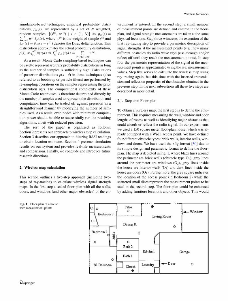
To obtain a wireless map, the first step is to define the envi-ronment. This requires measuring the wall, window and doorlengths of rooms as well as identifying major obstacles thatcould absorb or reflect the radio signal. In our experimentswe used a 150 square meter floor-plan house, which was al-ready equipped with a Wi-Fi access point. We have definedfour different obstacle types: brick walls, interior walls, win-dows and doors. We have used the xfig format [30] due toits simple design and parametric format to define the floor-plan. The map is depicted in Fig. 1, where black lines aroundthe perimeter are brick walls (obstacle type O1), grey linesaround the perimeter are windows (O2), grey lines insidethe house are interior walls (O3) and dark lines inside thehouse are doors (O4). Furthermore, the grey square indicatesthe location of the access point (in Bedroom 2) while thescattered small discs represent the measurement points to beused in the second step. The floor-plan could be enhancedby adding furniture locations and other objects. This would

Fig. 1 Floor-plan of a housewith measurement points

Springer

Wireless Networks

increase the complexity of the fourth step because the trans-mission and reflection parameters for these objects must alsobe calculated.

2.2. Step two: Measurement and measurement points

In the second step the user is required to define measurementpoints well-spread across the floor-plan (as represented bythe scattered discs in Fig. 1). The number of measurementpoints to be defined depends on the number of obstacles inthe floor-plan. To obtain good results, at least twice as manymeasurement points are needed as there are obstacle types(as explained in the next subsection). In our example wehave defined 10 measurement points (8 due to the 4 differentobstacle types and an additional 2 for increased precision).Note that the more measurement points we define the betterthe precision of the final map will be. An average signalstrength reading for each of the measurement points needs tobe taken and recorded. Let us denote the measurement pointsby M1. . .Mm, where m is the total number of measurementpoints. Furthermore, let us denote the power readings takenat these measurement points by WM1 . . . WMm .

In our example, several signal strength measurements ateach of the measurement points were taken using an OrinocoWi-Fi interface equipped, Linux managed laptop. Thesemeasurements were averaged for each measurement pointand stored for later use. Additionally, we have performedmeasurements to obtain no-obstacle one-meter distance sig-nal strength measurements for the access-point—wirelessnetwork adapter pair to be used as the calibration for stepfour; we will denote this measurement by P0.

2.3. Step three: Parametric ray-tracing

In this step we are running a “parametric” ray-tracing algo-rithm to find the signal strength of the access point at allthe measurement points as a function of the transmissionand reflection parameters of the obstacles. Wi-Fi works atthe 2.4 GHz frequency range, where the radio signal com-ing off the access point can be approximated with the sumof single straight-line propagation rays emanating in all di-rections around the omni-directional antenna of the accesspoint [11]. If a radio energy beam hits an obstacle, someportion of the energy of the beam is assumed to be reflected(bounce) and some portion of the energy is assumed to betransmitted (let through) by the obstacle. We denote the re-flection and transmission coefficients of the ith obstacle typeby ROi andTOi respectively, where

(ROi + TOi

)< 1. (Thus,

the obstacle is assumed to absorb 1 − (ROi + TOi

)portion of

the energy beam going through it). For example, if obstacle-1 is in the way of a traced radio ray, then it is assumedto reflect RO1 portion of the energy of the ray, while let-

ting TO1 portion of the same incoming energy propagatethrough.

Rays are generated starting from the access point in alldirections but to keep the process computationally feasi-ble, the direction of the rays has to be discretized between(0, 2 π ) with a �α precision. Thus, the resulting 2π /�α raysneed to be traced one-by-one sequentially. A ray crossing anobstacle will cease to exist but will spawn two other rays,one going on in the same direction (if the perimeter of thetarget area is not reached) and the other bouncing back fromthe obstacle. Each of these newly spawned rays will inheritproperties from its parent, such as the distance traveled, thenumber and type of obstacles it has already been reflectedand transmitted by. Each ray remains in the system until thetotal distance traveled by it reaches a pre-defined threshold.If a ray crosses the area of a measurement point, then itscurrent parameters (distance traveled, number and type ofdifferent transmissions and reflections) are stored for thatmeasurement point. Let us denote (i) the different types ofobstacles by O1. . .Ob; (ii) the number of reflections fromthese obstacles by r1. . .rb (e.g., ri corresponds to the numberof reflections from obstacle-type i, i.e., Oi); (iii) the numberof transmissions going through obstacles by t1. . .tb (e.g., ticorresponds to the number of transmissions by obstacle-typei, i.e., Oi); (iv) and the distance of travel by d. The power-footprint of a crossing ray at the measurement point is:

P0

d2

b∏

i=1

RriOi

∗b∏

i=1

T tiOi

.

Furthermore, let us denote the number of rays goingthrough the measurement points by NM1 . . . NMm respec-tively. Thus, for each of these points we have a polynomialdefining the received signal strength:

PM j =NM j∑

k=1

(P0

kd2

b∏

i=1

RkriOi

∗b∏

i=1

Tk tiOi

)

(1)

In Eq. (1), RO1 . . . ROb and TO1 . . . TOb are unknowns tobe determined, and upper-left indices represent ray indexesfor the kth ray (i.e.,kri is the number of reflections the kth rayhad encountered on obstacle-type (i). Thus by the end of thethird step for each measurement point we have a polynomialrepresentation of the total signal strength.

2.4. Step four: Obstacle parameter determination

The signal strength measurements obtained in the sec-ond step

(WM1 . . . WMm

)can now be used as estimates for

PM1 . . . PMm (i.e.,PM1 − WM1 , . . . , PMm − WMm should all beclose to zero). By looking at Eq. (1) we note that we have

Springer

Wireless Networks

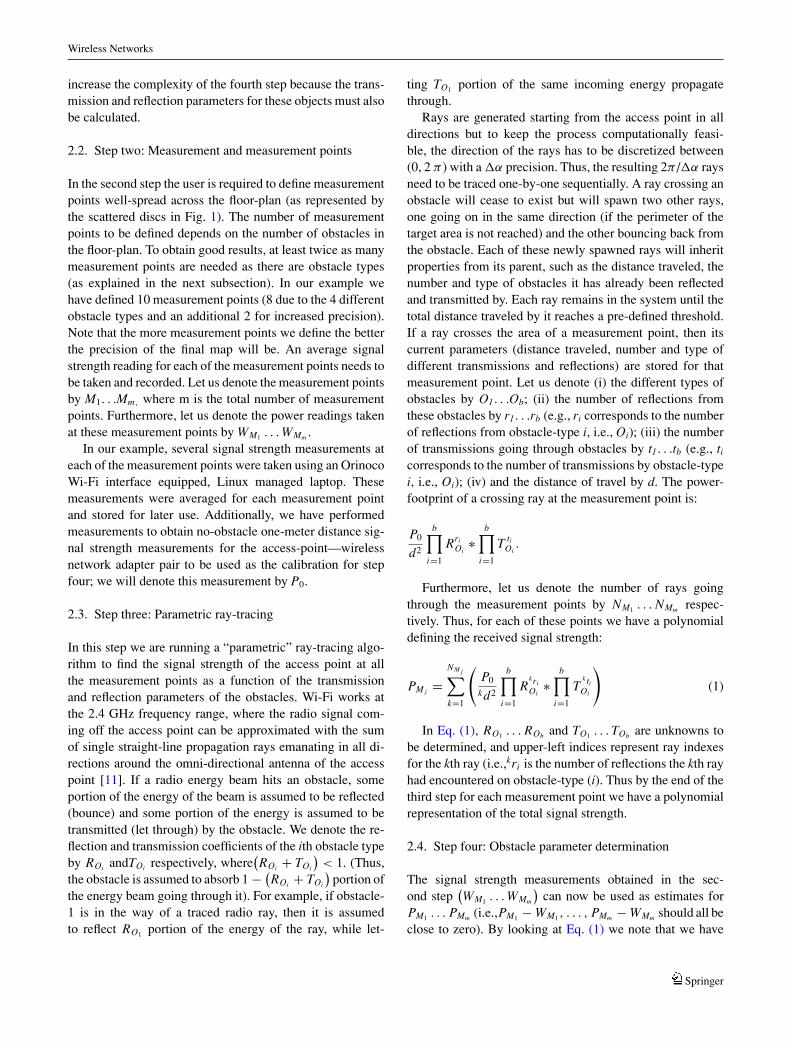
Fig. 2 Calculated wireless map

2b unknowns. In step-four we will estimate the values ofthese unknowns thus finding values for the reflection andtransmission parameters of all obstacle types. In order to beable to solve the above polynomials for the 2b unknowns,we need at least m ≥ 2b equations, i.e., m ≥ 2b measurementpoints. Due to the coarse modeling of the environment, wehave to also include an error term ei into the measurement.Then, for all i, where m ≥ i ≥ 1;WMi = PMi + ei . We cannow calculate a least square error estimate for all unknownsby minimizing the following function F:

F(RO1 . . . ROb , TO1 . . . TOb

) =m∑

j=1

e2j =

m∑

j=1

(WM j − PM j

)2

Minimization of function F is a complex problem dueto the number of variables and the order of the individualpolynomials. Thus, to minimize F we employ a heuristicoptimization technique, namely simulated annealing (SA)[15,19]. With simulated annealing, sub-optimal values forRO1 . . . ROb , and TO1 . . . TOb can be obtained (thus findingestimates on how what proportion of the energy reachingthe different obstacle types is reflected or transmitted). OurSA algorithm takes the polynomial description file generatedin the third step, the measured values for the measurementpoints, and P0 (obtained in the second step) as the input andprovides the estimated values for the reflection and transmis-sion parameters for all defined obstacles.

2.5. Step five: Ray-tracing for wireless power maps

In step five, the actual wireless power map is obtained usingthe previously calculated power reflection and transmissioncoefficients for the defined obstacles. The first task is to de-fine the angular precision of the ray-tracing by selecting anappropriate �α as well as defining the resolution of the wire-less power map by discretizing the target area into consecu-tive �s side-sized square cells. The selection of �s has littleimpact on the complexity of computation of the ray-tracingor the localization algorithms. However, �s has an impact

on the precision of the location estimate. The ray-tracingprocess is similar to that of the third step with the exceptionthat radio rays now leave a scalar power level footprint in allcells they travel through. Figure 2 shows a visualization ofthe wireless power map for our sample floor-plan, with �s= 0.3 m, where a darker cell indicates higher signal strength(the darkness of cells changes logarithmically in the powerlevel, since a dB scale is used to represent the values). Acomparison and discussion on the simulated and measuredpower levels can be found in Section 4.1.

3. Monte Carlo sampling-based bayesian-filtering

This section describes the basic approach to mobile nodelocalization from RSSI measurements and introduces fourestimation models that have been implemented and tested.Our goal is to obtain an estimate of the posterior probabilitydistribution, p(st | d1, . . . , dt ), of potential states (locations),st, using the RSSI measurements, d1, . . . , dt, and the wirelesspower map introduced in Section 2.

The calculation of the distribution of the user, given thesequence of RSSI readings is performed recursively using aBayes filter:

p(st | d1, . . . , dt )

= p(dt | st , d1, . . . , dt−1) · p(st | d1, . . . , dt−1)

p(dt | d1, . . . , dt−1)

Assuming that the Markov assumption holds, i.e., p(st |st−1, . . . , s0, dt−1, . . . , d1) = p(st | st−1), the filtering equa-tion can be transformed into the recursive form:

p(st | d1, . . . , dt )

= p(dt |st ) · ∫p(st |st−1) · p(st−1|d1, . . . , dt−1)dst−1

p(dt |d1, . . . , dt−1),

where p(dt | d1, . . . , dt−1) is a normalization constant. Inthe case of the localization of a mobile node from RSSImeasurements, the Markov assumption requires that the statecontains all available information that could assist in pre-dicting the next state and thus an estimate of the non-randommotion parameters of the node is required as part of thestate description. Starting with an initial, prior probabilitydistribution, p(s0),2 a system model, p(st | st−1), represent-ing the motion of the mobile node, and the measurementmodel, p(d | s), it is then possible to derive new estimatesof the probability distribution over time, integrating one new

2 A usual initial distribution is a uniform distribution, which means thatthe user is equally likely to be located at any part of the house in ourapplication.

Springer

Wireless Networks

measurement at a time. Each recursive update of the filtercan be broken into two stages:

Prediction: Use the system model to predict the state dis-tribution based on previous readings:

p(st |d1, . . . , dt−1)

=∫

p(st |st−1) · p(st−1|d1, . . . , dt−1)dst−1

Update: Use the measurement model to update the esti-mate:

p(st |d1, . . . , dt ) = p(dt |st )

p(dt |d1, . . . , dt−1)p(st |d1, . . . , dt−1)

To address the complexity of the integration step andthe problem of representing and updating a probabilityfunction defined on a continuous state space (which there-fore has an infinite number of states), the approach pre-sented here uses a sequential Monte Carlo filter to per-form Bayesian filtering on a sample representation. As in-troduced in Section 1.3, a distribution is represented by aset of weighted random samples and all filtering steps areperformed using Monte Carlo sampling operations. In par-ticular, the initial sample distribution, pN(s0), is representedby a set of uniformly distributed samples with equal weights,{(s(i)

0 , w(i)0 ) | i ∈ [1, N ], w(i)

0 = 1/N }, and the filtering stepsare performed as follows:

Prediction: For each sample, (s(i)t−1, w

(i)t−1), in the sample

set, randomly generate a replacement sample according tothe system model, p(st | st−1). This result in a new set ofsamples corresponding top(st |d1, . . . , dt−1):

{(s(i)

t , w(i)t

) ∣∣ i ∈ [1, N ], w(i)

t = 1/N}

Update: For each sample, (s(i)t , w

(i)t ), set the impor-

tance weight to the measurement probability of the ac-tual measurement, w(i)

t = p(dt | s(i)t ). Normalize the weights

such that∑

i∈[1,N ] η · w(i)t = 1.0 and draw N random sam-

ples for the sample set {(s(i)t , η · w(i)

t )|i ∈ [1, N ]} accord-ing to the normalized weight distribution. Set the weightsof the new samples to 1/N, resulting in a new set of sam-ples {(s(i)

t , w(i)t ) | i ∈ [1, N ], w(i)

t = 1/N } corresponding tothe posterior distributionp(st | d1, . . . , dt ).

To apply the filter to the problem of mobile node lo-calization from RSSI measurements, a system model and ameasurement model have to be provided. The latter is heregiven by the wireless power map introduced in Section 2 andthe assumption that actual RSSI readings will diverge fromthe map according to a Gaussian probability distributionwith a standard deviation of 3 dB. For the system model,

four different motion models have been implemented andtested in an example environment with a single wireless ac-cess point and no additional location information. The firstthree models assume that the receiving antenna of the en-tity to be located is always facing the access point (so thesimilarly calculated wireless map can be used without mod-ification), while the fourth model extends the framework todeal with users that may change their rotational directionrelative to the access point. The following sections intro-duce the individual movement models and their implica-tions for the Monte Carlo filter before they are evaluated inSection 4.

3.1. Simple sequential Monte Carlo filter

The simplest localization algorithm tested here uses a sys-tem model that assumes that at every point in time, the nodemoves with a random velocity drawn from a normal distri-bution with a mean of 0 m/s and a standard deviation of1 m/s, vt ∼ N(0, 1). This model corresponds to a randomdisplacement of the mobile node at every point in time. Noinformation about the environment is included in this model,and as a consequence, the filter permits the estimates to movealong arbitrary paths (including ones that move through thewalls). Since this motion model also does not consider anypast motions (i.e., it does not estimate the speed and/or ac-celeration of the user), the state of the localization filter canbe represented as a vector of the x and y location, s = (xy)T ,while the measurements d correspond to RSSI measurementsin dB.

3.2. Simple sequential Monte Carlo filter withboundary information

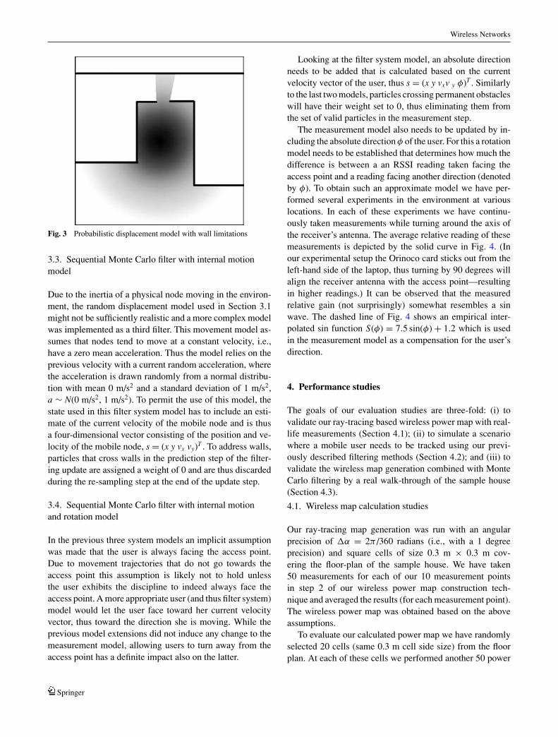
To model the effects of boundaries and limit the simulatedsample trajectories to physically possible ones, the secondfilter uses information about the location of the walls tomodify the Gaussian velocity model by limiting availablechoices to velocities that do not lead to collisions with per-manent obstacles (such as windows or walls). Figure 3 showsan example for this motion model, which corresponds to arandom displacement limited by the walls. The figure showsthe probability density of moving to a new location withinone time step assuming that the mobile node is located at thecenter of the distribution. Dark regions correspond to highprobabilities while light colors represent low displacementprobabilities (dark lines indicate walls).

Similarly to the simplest system model of Section 3.1,this filter system model uses a two-dimensional state vector,s = (xy)T , and measurements, d, corresponding to the RSSIreadings.

Springer

Wireless Networks

Fig. 3 Probabilistic displacement model with wall limitations

3.3. Sequential Monte Carlo filter with internal motionmodel

Due to the inertia of a physical node moving in the environ-ment, the random displacement model used in Section 3.1might not be sufficiently realistic and a more complex modelwas implemented as a third filter. This movement model as-sumes that nodes tend to move at a constant velocity, i.e.,have a zero mean acceleration. Thus the model relies on theprevious velocity with a current random acceleration, wherethe acceleration is drawn randomly from a normal distribu-tion with mean 0 m/s2 and a standard deviation of 1 m/s2,a ∼ N(0 m/s2, 1 m/s2). To permit the use of this model, thestate used in this filter system model has to include an esti-mate of the current velocity of the mobile node and is thusa four-dimensional vector consisting of the position and ve-locity of the mobile node, s = (x y vx vy)T . To address walls,particles that cross walls in the prediction step of the filter-ing update are assigned a weight of 0 and are thus discardedduring the re-sampling step at the end of the update step.

3.4. Sequential Monte Carlo filter with internal motionand rotation model

In the previous three system models an implicit assumptionwas made that the user is always facing the access point.Due to movement trajectories that do not go towards theaccess point this assumption is likely not to hold unlessthe user exhibits the discipline to indeed always face theaccess point. A more appropriate user (and thus filter system)model would let the user face toward her current velocityvector, thus toward the direction she is moving. While theprevious model extensions did not induce any change to themeasurement model, allowing users to turn away from theaccess point has a definite impact also on the latter.

Looking at the filter system model, an absolute directionneeds to be added that is calculated based on the currentvelocity vector of the user, thus s = (x y vxv y φ)T . Similarlyto the last two models, particles crossing permanent obstacleswill have their weight set to 0, thus eliminating them fromthe set of valid particles in the measurement step.

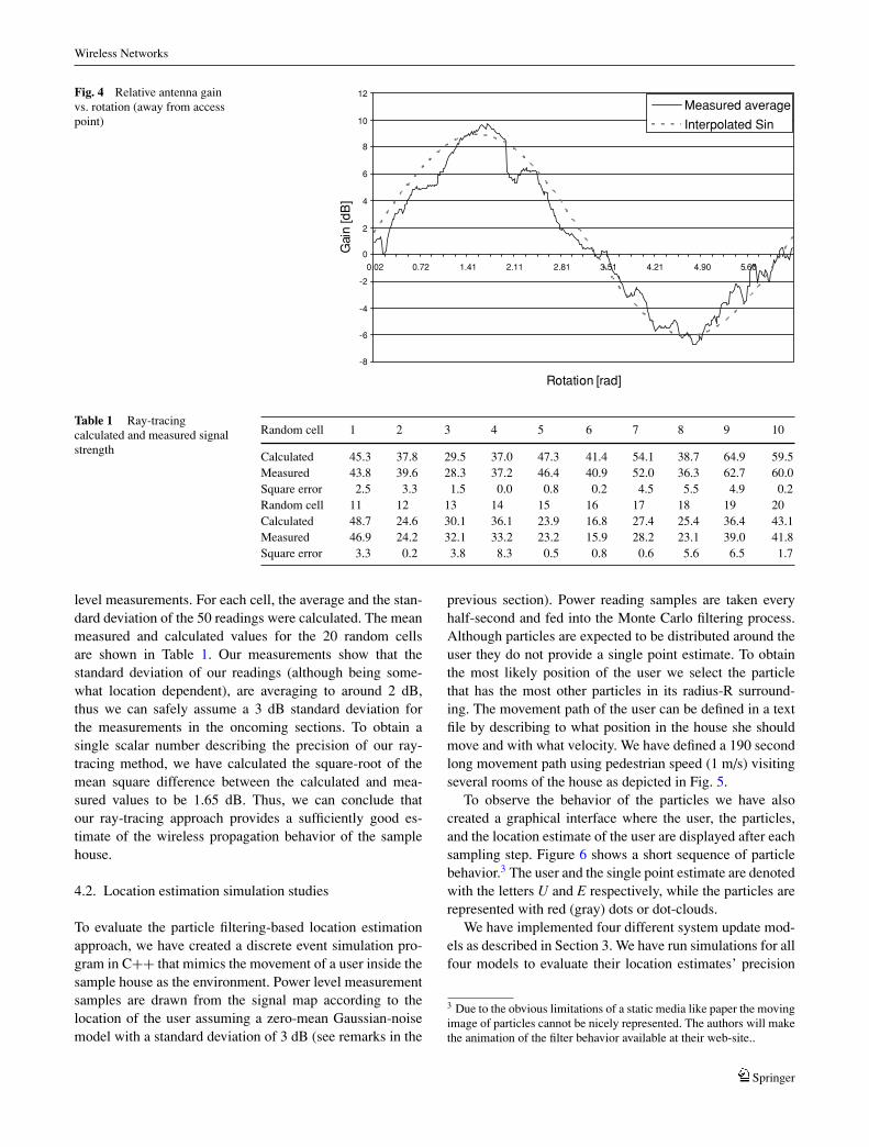
The measurement model also needs to be updated by in-cluding the absolute direction φ of the user. For this a rotationmodel needs to be established that determines how much thedifference is between a an RSSI reading taken facing theaccess point and a reading facing another direction (denotedby φ). To obtain such an approximate model we have per-formed several experiments in the environment at variouslocations. In each of these experiments we have continu-ously taken measurements while turning around the axis ofthe receiver’s antenna. The average relative reading of thesemeasurements is depicted by the solid curve in Fig. 4. (Inour experimental setup the Orinoco card sticks out from theleft-hand side of the laptop, thus turning by 90 degrees willalign the receiver antenna with the access point—resultingin higher readings.) It can be observed that the measuredrelative gain (not surprisingly) somewhat resembles a sinwave. The dashed line of Fig. 4 shows an empirical inter-polated sin function S(φ) = 7.5 sin(φ) + 1.2 which is usedin the measurement model as a compensation for the user’sdirection.

4. Performance studies

The goals of our evaluation studies are three-fold: (i) tovalidate our ray-tracing based wireless power map with real-life measurements (Section 4.1); (ii) to simulate a scenariowhere a mobile user needs to be tracked using our previ-ously described filtering methods (Section 4.2); and (iii) tovalidate the wireless map generation combined with MonteCarlo filtering by a real walk-through of the sample house(Section 4.3).

4.1. Wireless map calculation studies

Our ray-tracing map generation was run with an angularprecision of �α = 2π /360 radians (i.e., with a 1 degreeprecision) and square cells of size 0.3 m × 0.3 m cov-ering the floor-plan of the sample house. We have taken50 measurements for each of our 10 measurement pointsin step 2 of our wireless power map construction tech-nique and averaged the results (for each measurement point).The wireless power map was obtained based on the aboveassumptions.

To evaluate our calculated power map we have randomlyselected 20 cells (same 0.3 m cell side size) from the floorplan. At each of these cells we performed another 50 power

Springer

Wireless Networks

-8

-6

-4

-2

0

2

4

6

8

10

12

0.02 0.72 1.41 2.11 2.81 3.51 4.21 4.90 5.60

Rotation [rad]

Gai

n [d

B]

Measured average

Interpolated Sin

Fig. 4 Relative antenna gainvs. rotation (away from accesspoint)

Table 1 Ray-tracingcalculated and measured signalstrength

Random cell 1 2 3 4 5 6 7 8 9 10

Calculated 45.3 37.8 29.5 37.0 47.3 41.4 54.1 38.7 64.9 59.5Measured 43.8 39.6 28.3 37.2 46.4 40.9 52.0 36.3 62.7 60.0Square error 2.5 3.3 1.5 0.0 0.8 0.2 4.5 5.5 4.9 0.2Random cell 11 12 13 14 15 16 17 18 19 20Calculated 48.7 24.6 30.1 36.1 23.9 16.8 27.4 25.4 36.4 43.1Measured 46.9 24.2 32.1 33.2 23.2 15.9 28.2 23.1 39.0 41.8Square error 3.3 0.2 3.8 8.3 0.5 0.8 0.6 5.6 6.5 1.7

level measurements. For each cell, the average and the stan-dard deviation of the 50 readings were calculated. The meanmeasured and calculated values for the 20 random cellsare shown in Table 1. Our measurements show that thestandard deviation of our readings (although being some-what location dependent), are averaging to around 2 dB,thus we can safely assume a 3 dB standard deviation forthe measurements in the oncoming sections. To obtain asingle scalar number describing the precision of our ray-tracing method, we have calculated the square-root of themean square difference between the calculated and mea-sured values to be 1.65 dB. Thus, we can conclude thatour ray-tracing approach provides a sufficiently good es-timate of the wireless propagation behavior of the samplehouse.

4.2. Location estimation simulation studies

To evaluate the particle filtering-based location estimationapproach, we have created a discrete event simulation pro-gram in C++ that mimics the movement of a user inside thesample house as the environment. Power level measurementsamples are drawn from the signal map according to thelocation of the user assuming a zero-mean Gaussian-noisemodel with a standard deviation of 3 dB (see remarks in the

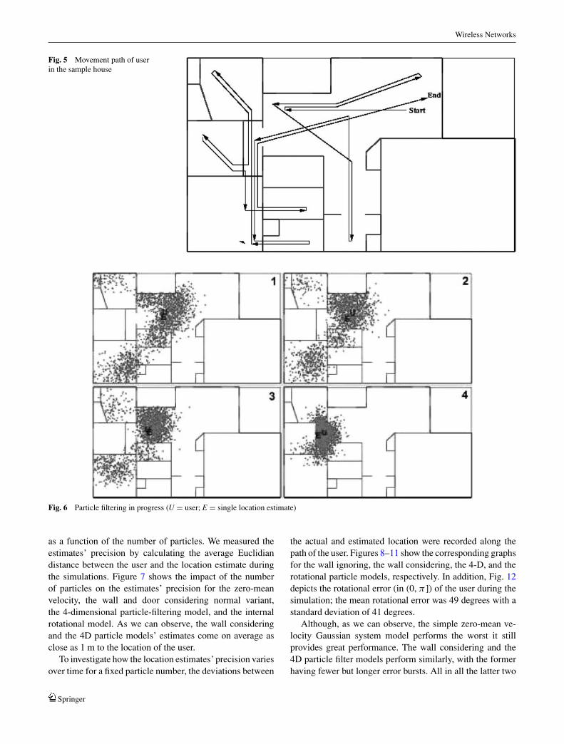
previous section). Power reading samples are taken everyhalf-second and fed into the Monte Carlo filtering process.Although particles are expected to be distributed around theuser they do not provide a single point estimate. To obtainthe most likely position of the user we select the particlethat has the most other particles in its radius-R surround-ing. The movement path of the user can be defined in a textfile by describing to what position in the house she shouldmove and with what velocity. We have defined a 190 secondlong movement path using pedestrian speed (1 m/s) visitingseveral rooms of the house as depicted in Fig. 5.

To observe the behavior of the particles we have alsocreated a graphical interface where the user, the particles,and the location estimate of the user are displayed after eachsampling step. Figure 6 shows a short sequence of particlebehavior.3 The user and the single point estimate are denotedwith the letters U and E respectively, while the particles arerepresented with red (gray) dots or dot-clouds.

We have implemented four different system update mod-els as described in Section 3. We have run simulations for allfour models to evaluate their location estimates’ precision

3 Due to the obvious limitations of a static media like paper the movingimage of particles cannot be nicely represented. The authors will makethe animation of the filter behavior available at their web-site..

Springer

Wireless Networks

Fig. 5 Movement path of userin the sample house

Fig. 6 Particle filtering in progress (U = user; E = single location estimate)

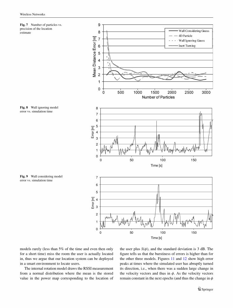
as a function of the number of particles. We measured theestimates’ precision by calculating the average Euclidiandistance between the user and the location estimate duringthe simulations. Figure 7 shows the impact of the numberof particles on the estimates’ precision for the zero-meanvelocity, the wall and door considering normal variant,the 4-dimensional particle-filtering model, and the internalrotational model. As we can observe, the wall consideringand the 4D particle models’ estimates come on average asclose as 1 m to the location of the user.

To investigate how the location estimates’ precision variesover time for a fixed particle number, the deviations between

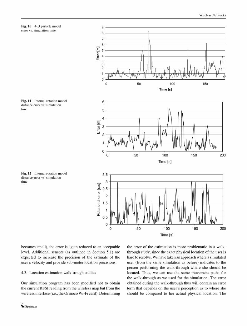
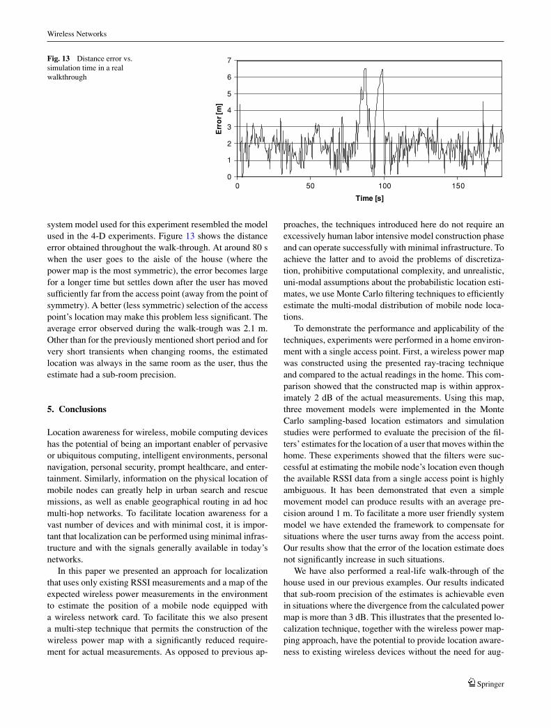
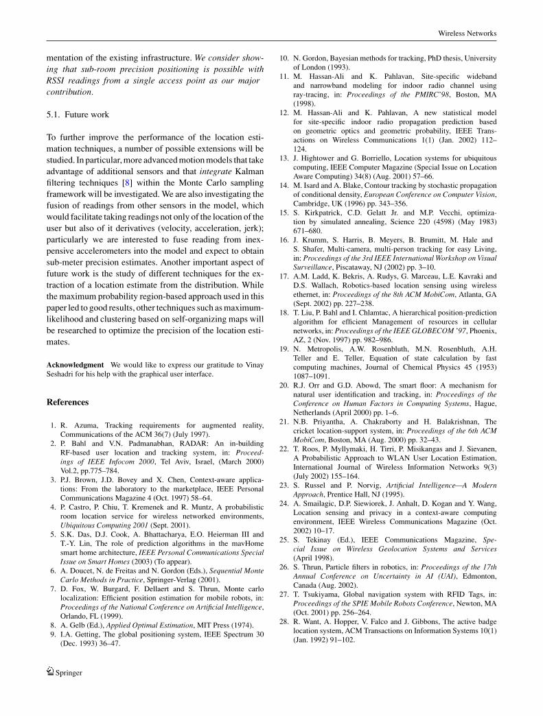
the actual and estimated location were recorded along thepath of the user. Figures 8–11 show the corresponding graphsfor the wall ignoring, the wall considering, the 4-D, and therotational particle models, respectively. In addition, Fig. 12depicts the rotational error (in (0, π ]) of the user during thesimulation; the mean rotational error was 49 degrees with astandard deviation of 41 degrees.

Although, as we can observe, the simple zero-mean ve-locity Gaussian system model performs the worst it stillprovides great performance. The wall considering and the4D particle filter models perform similarly, with the formerhaving fewer but longer error bursts. All in all the latter two

Springer

Wireless Networks

Fig. 7 Number of particles vs.precision of the locationestimate

0

1

2

3

4

5

6

7

8

0 50 100 150

Time [s]

Err

or [m

]

Fig. 8 Wall ignoring modelerror vs. simulation time

0

1

2

3

4

5

6

7

0 50 100 150

Time [s]

Err

or [m

]

Fig. 9 Wall considering modelerror vs. simulation time

models rarely (less than 5% of the time and even then onlyfor a short time) miss the room the user is actually locatedin, thus we argue that our location system can be deployedin a smart environment to locate users.

The internal rotation model draws the RSSI measurementfrom a normal distribution where the mean is the storedvalue in the power map corresponding to the location of

the user plus S(φ), and the standard deviation is 3 dB. Thefigure tells us that the burstiness of errors is higher than forthe other three models. Figures 11 and 12 show high errorpeaks at times where the simulated user has abruptly turnedits direction, i.e., when there was a sudden large change inthe velocity vectors and thus in φ. As the velocity vectorsremain constant in the next epochs (and thus the change in φ

Springer

Wireless Networks

0

1

2

3

4

5

6

7

8

9

0 50 100 150

Time [s]

Err

or [

m]

Fig. 10 4-D particle modelerror vs. simulation time

0

1

2

3

4

5

6

0 50 100 150 200

Time [s]

Err

or [

m]

Fig. 11 Internal rotation modeldistance error vs. simulationtime

0

0.5

1

1.5

2

2.5

3

3.5

0 50 100 150 200

Time [s]

Rot

atio

nal e

rror

[ra

d]

Fig. 12 Internal rotation modeldistance error vs. simulationtime

becomes small), the error is again reduced to an acceptablelevel. Additional sensors (as outlined in Section 5.1) areexpected to increase the precision of the estimate of theuser’s velocity and provide sub-meter location precisions.

4.3. Location estimation walk-trough studies

Our simulation program has been modified not to obtainthe current RSSI reading from the wireless map but from thewireless interface (i.e., the Orinoco Wi-Fi card). Determining

the error of the estimation is more problematic in a walk-through study, since the exact physical location of the user ishard to resolve. We have taken an approach where a simulateduser (from the same simulation as before) indicates to theperson performing the walk-through where she should belocated. Thus, we can use the same movement paths forthe walk-through as we used for the simulation. The errorobtained during the walk-through thus will contain an errorterm that depends on the user’s perception as to where sheshould be compared to her actual physical location. The

Springer

Wireless Networks

0

1

2

3

4

5

6

7

0 50 100 150

Time [s]

Err

or [

m]

Fig. 13 Distance error vs.simulation time in a realwalkthrough

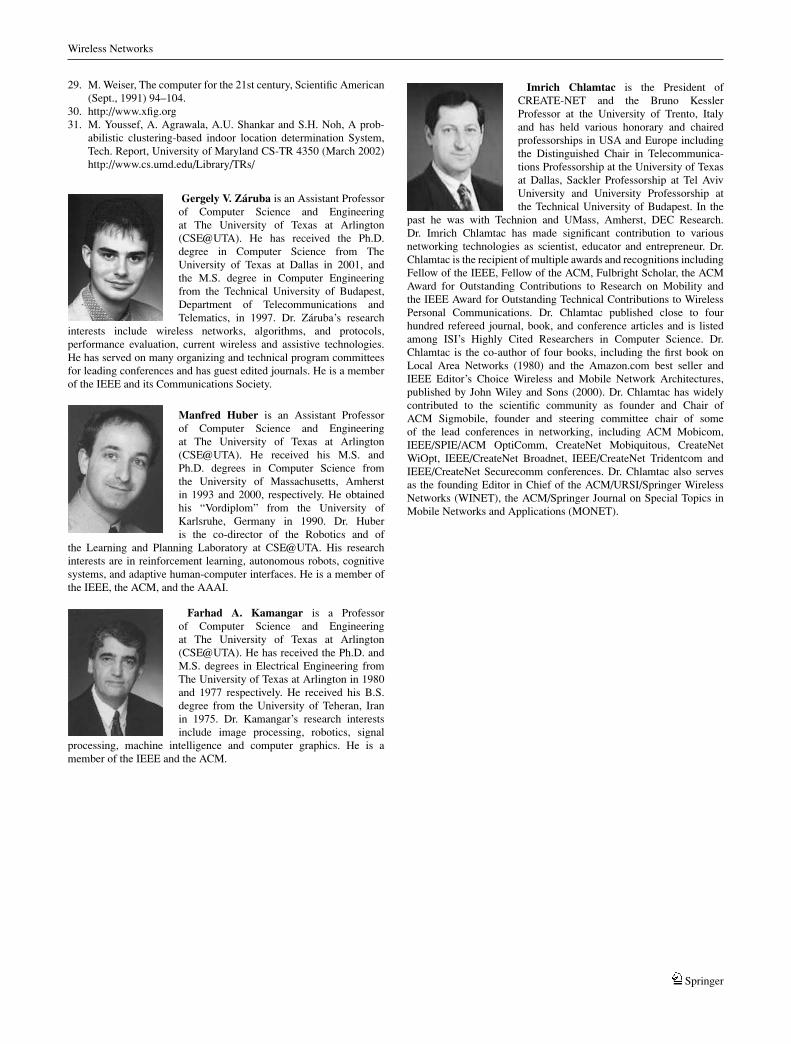
system model used for this experiment resembled the modelused in the 4-D experiments. Figure 13 shows the distanceerror obtained throughout the walk-through. At around 80 swhen the user goes to the aisle of the house (where thepower map is the most symmetric), the error becomes largefor a longer time but settles down after the user has movedsufficiently far from the access point (away from the point ofsymmetry). A better (less symmetric) selection of the accesspoint’s location may make this problem less significant. Theaverage error observed during the walk-trough was 2.1 m.Other than for the previously mentioned short period and forvery short transients when changing rooms, the estimatedlocation was always in the same room as the user, thus theestimate had a sub-room precision.

5. Conclusions

Location awareness for wireless, mobile computing deviceshas the potential of being an important enabler of pervasiveor ubiquitous computing, intelligent environments, personalnavigation, personal security, prompt healthcare, and enter-tainment. Similarly, information on the physical location ofmobile nodes can greatly help in urban search and rescuemissions, as well as enable geographical routing in ad hocmulti-hop networks. To facilitate location awareness for avast number of devices and with minimal cost, it is impor-tant that localization can be performed using minimal infras-tructure and with the signals generally available in today’snetworks.

In this paper we presented an approach for localizationthat uses only existing RSSI measurements and a map of theexpected wireless power measurements in the environmentto estimate the position of a mobile node equipped witha wireless network card. To facilitate this we also presenta multi-step technique that permits the construction of thewireless power map with a significantly reduced require-ment for actual measurements. As opposed to previous ap-

proaches, the techniques introduced here do not require anexcessively human labor intensive model construction phaseand can operate successfully with minimal infrastructure. Toachieve the latter and to avoid the problems of discretiza-tion, prohibitive computational complexity, and unrealistic,uni-modal assumptions about the probabilistic location esti-mates, we use Monte Carlo filtering techniques to efficientlyestimate the multi-modal distribution of mobile node loca-tions.

To demonstrate the performance and applicability of thetechniques, experiments were performed in a home environ-ment with a single access point. First, a wireless power mapwas constructed using the presented ray-tracing techniqueand compared to the actual readings in the home. This com-parison showed that the constructed map is within approx-imately 2 dB of the actual measurements. Using this map,three movement models were implemented in the MonteCarlo sampling-based location estimators and simulationstudies were performed to evaluate the precision of the fil-ters’ estimates for the location of a user that moves within thehome. These experiments showed that the filters were suc-cessful at estimating the mobile node’s location even thoughthe available RSSI data from a single access point is highlyambiguous. It has been demonstrated that even a simplemovement model can produce results with an average pre-cision around 1 m. To facilitate a more user friendly systemmodel we have extended the framework to compensate forsituations where the user turns away from the access point.Our results show that the error of the location estimate doesnot significantly increase in such situations.

We have also performed a real-life walk-through of thehouse used in our previous examples. Our results indicatedthat sub-room precision of the estimates is achievable evenin situations where the divergence from the calculated powermap is more than 3 dB. This illustrates that the presented lo-calization technique, together with the wireless power map-ping approach, have the potential to provide location aware-ness to existing wireless devices without the need for aug-

Springer

Wireless Networks

mentation of the existing infrastructure. We consider show-ing that sub-room precision positioning is possible withRSSI readings from a single access point as our majorcontribution.

5.1. Future work

To further improve the performance of the location esti-mation techniques, a number of possible extensions will bestudied. In particular, more advanced motion models that takeadvantage of additional sensors and that integrate Kalmanfiltering techniques [8] within the Monte Carlo samplingframework will be investigated. We are also investigating thefusion of readings from other sensors in the model, whichwould facilitate taking readings not only of the location of theuser but also of it derivatives (velocity, acceleration, jerk);particularly we are interested to fuse reading from inex-pensive accelerometers into the model and expect to obtainsub-meter precision estimates. Another important aspect offuture work is the study of different techniques for the ex-traction of a location estimate from the distribution. Whilethe maximum probability region-based approach used in thispaper led to good results, other techniques such as maximum-likelihood and clustering based on self-organizing maps willbe researched to optimize the precision of the location esti-mates.

Acknowledgment We would like to express our gratitude to VinaySeshadri for his help with the graphical user interface.

References

1. R. Azuma, Tracking requirements for augmented reality,Communications of the ACM 36(7) (July 1997).

2. P. Bahl and V.N. Padmanabhan, RADAR: An in-buildingRF-based user location and tracking system, in: Proceed-ings of IEEE Infocom 2000, Tel Aviv, Israel, (March 2000)Vol.2, pp.775–784.

3. P.J. Brown, J.D. Bovey and X. Chen, Context-aware applica-tions: From the laboratory to the marketplace, IEEE PersonalCommunications Magazine 4 (Oct. 1997) 58–64.

4. P. Castro, P. Chiu, T. Kremenek and R. Muntz, A probabilisticroom location service for wireless networked environments,Ubiquitous Computing 2001 (Sept. 2001).

5. S.K. Das, D.J. Cook, A. Bhattacharya, E.O. Heierman III andT.-Y. Lin, The role of prediction algorithms in the mavHomesmart home architecture, IEEE Personal Communications SpecialIssue on Smart Homes (2003) (To appear).

6. A. Doucet, N. de Freitas and N. Gordon (Eds.), Sequential MonteCarlo Methods in Practice, Springer-Verlag (2001).

7. D. Fox, W. Burgard, F. Dellaert and S. Thrun, Monte carlolocalization: Efficient position estimation for mobile robots, in:Proceedings of the National Conference on Artificial Intelligence,Orlando, FL (1999).

8. A. Gelb (Ed.), Applied Optimal Estimation, MIT Press (1974).9. I.A. Getting, The global positioning system, IEEE Spectrum 30

(Dec. 1993) 36–47.

10. N. Gordon, Bayesian methods for tracking, PhD thesis, Universityof London (1993).

11. M. Hassan-Ali and K. Pahlavan, Site-specific widebandand narrowband modeling for indoor radio channel usingray-tracing, in: Proceedings of the PMIRC’98, Boston, MA(1998).

12. M. Hassan-Ali and K. Pahlavan, A new statistical modelfor site-specific indoor radio propagation prediction basedon geometric optics and geometric probability, IEEE Trans-actions on Wireless Communications 1(1) (Jan. 2002) 112–124.

13. J. Hightower and G. Borriello, Location systems for ubiquitouscomputing, IEEE Computer Magazine (Special Issue on LocationAware Computing) 34(8) (Aug. 2001) 57–66.

14. M. Isard and A. Blake, Contour tracking by stochastic propagationof conditional density, European Conference on Computer Vision,Cambridge, UK (1996) pp. 343–356.

15. S. Kirkpatrick, C.D. Gelatt Jr. and M.P. Vecchi, optimiza-tion by simulated annealing, Science 220 (4598) (May 1983)671–680.

16. J. Krumm, S. Harris, B. Meyers, B. Brumitt, M. Hale andS. Shafer, Multi-camera, multi-person tracking for easy Living,in: Proceedings of the 3rd IEEE International Workshop on VisualSurveillance, Piscataway, NJ (2002) pp. 3–10.

17. A.M. Ladd, K. Bekris, A. Rudys, G. Marceau, L.E. Kavraki andD.S. Wallach, Robotics-based location sensing using wirelessethernet, in: Proceedings of the 8th ACM MobiCom, Atlanta, GA(Sept. 2002) pp. 227–238.

18. T. Liu, P. Bahl and I. Chlamtac, A hierarchical position-predictionalgorithm for efficient Management of resources in cellularnetworks, in: Proceedings of the IEEE GLOBECOM ’97, Phoenix,AZ, 2 (Nov. 1997) pp. 982–986.

19. N. Metropolis, A.W. Rosenbluth, M.N. Rosenbluth, A.H.Teller and E. Teller, Equation of state calculation by fastcomputing machines, Journal of Chemical Physics 45 (1953)1087–1091.

20. R.J. Orr and G.D. Abowd, The smart floor: A mechanism fornatural user identification and tracking, in: Proceedings of theConference on Human Factors in Computing Systems, Hague,Netherlands (April 2000) pp. 1–6.

21. N.B. Priyantha, A. Chakraborty and H. Balakrishnan, Thecricket location-support system, in: Proceedings of the 6th ACMMobiCom, Boston, MA (Aug. 2000) pp. 32–43.

22. T. Roos, P. Myllymaki, H. Tirri, P. Misikangas and J. Sievanen,A Probabilistic Approach to WLAN User Location Estimation,International Journal of Wireless Information Networks 9(3)(July 2002) 155–164.

23. S. Russel and P. Norvig, Artificial Intelligence—A ModernApproach, Prentice Hall, NJ (1995).

24. A. Smailagic, D.P. Siewiorek, J. Anhalt, D. Kogan and Y. Wang,Location sensing and privacy in a context-aware computingenvironment, IEEE Wireless Communications Magazine (Oct.2002) 10–17.

25. S. Tekinay (Ed.), IEEE Communications Magazine, Spe-cial Issue on Wireless Geolocation Systems and Services(April 1998).

26. S. Thrun, Particle filters in robotics, in: Proceedings of the 17thAnnual Conference on Uncertainty in AI (UAI), Edmonton,Canada (Aug. 2002).

27. T. Tsukiyama, Global navigation system with RFID Tags, in:Proceedings of the SPIE Mobile Robots Conference, Newton, MA(Oct. 2001) pp. 256–264.

28. R. Want, A. Hopper, V. Falco and J. Gibbons, The active badgelocation system, ACM Transactions on Information Systems 10(1)(Jan. 1992) 91–102.

Springer

Wireless Networks

29. M. Weiser, The computer for the 21st century, Scientific American(Sept., 1991) 94–104.

30. http://www.xfig.org31. M. Youssef, A. Agrawala, A.U. Shankar and S.H. Noh, A prob-

abilistic clustering-based indoor location determination System,Tech. Report, University of Maryland CS-TR 4350 (March 2002)http://www.cs.umd.edu/Library/TRs/

Gergely V. Zaruba is an Assistant Professorof Computer Science and Engineeringat The University of Texas at Arlington(CSE@UTA). He has received the Ph.D.degree in Computer Science from TheUniversity of Texas at Dallas in 2001, andthe M.S. degree in Computer Engineeringfrom the Technical University of Budapest,Department of Telecommunications andTelematics, in 1997. Dr. Zaruba’s research

interests include wireless networks, algorithms, and protocols,performance evaluation, current wireless and assistive technologies.He has served on many organizing and technical program committeesfor leading conferences and has guest edited journals. He is a memberof the IEEE and its Communications Society.

Manfred Huber is an Assistant Professorof Computer Science and Engineeringat The University of Texas at Arlington(CSE@UTA). He received his M.S. andPh.D. degrees in Computer Science fromthe University of Massachusetts, Amherstin 1993 and 2000, respectively. He obtainedhis “Vordiplom” from the University ofKarlsruhe, Germany in 1990. Dr. Huberis the co-director of the Robotics and of

the Learning and Planning Laboratory at CSE@UTA. His researchinterests are in reinforcement learning, autonomous robots, cognitivesystems, and adaptive human-computer interfaces. He is a member ofthe IEEE, the ACM, and the AAAI.

Farhad A. Kamangar is a Professorof Computer Science and Engineeringat The University of Texas at Arlington(CSE@UTA). He has received the Ph.D. andM.S. degrees in Electrical Engineering fromThe University of Texas at Arlington in 1980and 1977 respectively. He received his B.S.degree from the University of Teheran, Iranin 1975. Dr. Kamangar’s research interestsinclude image processing, robotics, signal

processing, machine intelligence and computer graphics. He is amember of the IEEE and the ACM.

Imrich Chlamtac is the President ofCREATE-NET and the Bruno KesslerProfessor at the University of Trento, Italyand has held various honorary and chairedprofessorships in USA and Europe includingthe Distinguished Chair in Telecommunica-tions Professorship at the University of Texasat Dallas, Sackler Professorship at Tel AvivUniversity and University Professorship atthe Technical University of Budapest. In the

past he was with Technion and UMass, Amherst, DEC Research.Dr. Imrich Chlamtac has made significant contribution to variousnetworking technologies as scientist, educator and entrepreneur. Dr.Chlamtac is the recipient of multiple awards and recognitions includingFellow of the IEEE, Fellow of the ACM, Fulbright Scholar, the ACMAward for Outstanding Contributions to Research on Mobility andthe IEEE Award for Outstanding Technical Contributions to WirelessPersonal Communications. Dr. Chlamtac published close to fourhundred refereed journal, book, and conference articles and is listedamong ISI’s Highly Cited Researchers in Computer Science. Dr.Chlamtac is the co-author of four books, including the first book onLocal Area Networks (1980) and the Amazon.com best seller andIEEE Editor’s Choice Wireless and Mobile Network Architectures,published by John Wiley and Sons (2000). Dr. Chlamtac has widelycontributed to the scientific community as founder and Chair ofACM Sigmobile, founder and steering committee chair of someof the lead conferences in networking, including ACM Mobicom,IEEE/SPIE/ACM OptiComm, CreateNet Mobiquitous, CreateNetWiOpt, IEEE/CreateNet Broadnet, IEEE/CreateNet Tridentcom andIEEE/CreateNet Securecomm conferences. Dr. Chlamtac also servesas the founding Editor in Chief of the ACM/URSI/Springer WirelessNetworks (WINET), the ACM/Springer Journal on Special Topics inMobile Networks and Applications (MONET).

Springer