Indoor Localization Based on RadioChannel Parameters in Wireless Sensor

Networks

JOSE ANTONIO GUTIERREZ GARCIA

Master’s Degree ProjectStockholm, Sweden

XR-EE-RT 2012:033

Indoor Localization Based on Radio Channel

Parameters in Wireless Sensor Networks

Jose Antonio Gutierrez Garcıa<jagg@kth.se>

December 16, 2012

Abstract

Wireless Sensor Networks are nowadays becoming increasingly popular. Dueto their low cost, ease of deployment and application, they offer robust so-lutions in a variety of fields. In this context, localization is one of the mostimportant functionalities that can be implemented. The analysis of exist-ing antennas that could suit a light, small, and energy-efficient sensor andthe analysis and design of localization algorithms have been studied in thiswork. Indoor localization in a smart home poses certain challenges in com-parison with the existing and successfully implemented large scale outdoorlocalization systems, due to the shadow fading effects and the notable differ-ences among the indoor environments. This work has focused on localizationbased on channel parameters estimation and received signal strength. Thisoffers versatility, since no previous knowledge of the indoor environment isrequired, and cheap deployment. A review of existing methods in this areais offered and two classical and robust approaches, least squares estimationand log-likelihood maximization are combined to obtain new algorithms thatcan statistically improve the performance in terms of bias and variance ofthe error. The results of this work can be applied to the development ofcheap and robustly optimized algorithms. Furthermore, the analysis of theantennas for this context sets the needs that new lines of future investigationand development of sensor devices can address.

Sammanfattning

Nufortiden blir Tradlosa Sensornatverk popularare. Pa grund av sin lagakostnad, enkel installation och tillampning, erbjuder de robusta losningarinom olika omraden. I detta sammanhang, ar lokalisering en av de viktigas-te funktionerna som kan genomforas. Analysen av befintliga antenner somkan passa en latt, liten och energisnal sensor och analysen och utformningenav lokalisering algoritmer har studerats i detta arbete. Inomhus lokalise-ring i ett smart hem innebar vissa utmaningar i jamforelse med befintligaoch framgangsrikt genomforta storskaliga utomhus system for lokalisering,pa grund av blekning effekter och de anmarkningsvarda skillnaderna mellaninomhusmiljoer. I denna mening har detta arbete fokuserat pa lokaliseringbaserad pa kanal parametrar uppskattning och mottagen signalstyrka. Dettager mangsidighet, eftersom inte nagon tidigare kunskap om inomhusmiljonkravs, och billig distribution. En oversyn av befintliga metoder inom dettaomrade erbjuds och tva klassiska och robusta metoder, minsta kvadratme-tod uppskattning och log-sannolikhet maximering kombineras for att fa nyaalgoritmer som statistiskt kan forbattra prestanda i fraga om partiskhet ochvarians av felet. Resultaten av detta arbete kan tillampas pa utveckling-en av billiga och robust optimerade algoritmer. Vidare faststaller analysenav antennerna for detta sammanhang de behov som nya linjer for framtidaundersokningar och utveckling av sensoranordningar kan hantera.

Contents

1 Introduction 11.1 Problem Definition . . . . . . . . . . . . . . . . . . . . . . . . 11.2 Goals . . . . . . . . . . . . . . . . . . . . . . . . . . . . . . . 21.3 Background . . . . . . . . . . . . . . . . . . . . . . . . . . . . 3

1.3.1 Present Situation of Localization in Wireless SensorNetworks (WSNs) . . . . . . . . . . . . . . . . . . . . 3

1.3.2 Present Situation of Energy Requirements in WSNs . 51.3.3 Main Standards and Specifications . . . . . . . . . . . 6

2 Overview on Suitable Antennas 82.1 Antenna Requirements . . . . . . . . . . . . . . . . . . . . . . 82.2 Comparative Study . . . . . . . . . . . . . . . . . . . . . . . . 10

2.2.1 2.4 GHz Antennas . . . . . . . . . . . . . . . . . . . . 102.2.2 UHF Radio-frequency identification (RFID) Antennas 112.2.3 Antennas Comparison . . . . . . . . . . . . . . . . . . 112.2.4 Harvesters . . . . . . . . . . . . . . . . . . . . . . . . . 12

3 Modelling of the Indoor Wireless Radio Channels 143.1 General Indoor Path Loss Propagation Models . . . . . . . . 14

3.1.1 The ITU Indoor Path Loss Model . . . . . . . . . . . 153.1.2 The Log-Distance Path Loss Model . . . . . . . . . . . 153.1.3 Indoor Attenuation Factors . . . . . . . . . . . . . . . 153.1.4 Simplified Path Loss Model . . . . . . . . . . . . . . . 163.1.5 Motley-Keenan Model . . . . . . . . . . . . . . . . . . 163.1.6 Multi-Wall-and-Floor . . . . . . . . . . . . . . . . . . 173.1.7 Shadow Fading . . . . . . . . . . . . . . . . . . . . . . 173.1.8 Other Indoor Path Loss Models . . . . . . . . . . . . . 17

3.2 General Indoor Fading Models . . . . . . . . . . . . . . . . . 173.2.1 Various Characteristics . . . . . . . . . . . . . . . . . 183.2.2 Saleh and Valenzuela Indoor Statistical Model . . . . 193.2.3 ∆-K . . . . . . . . . . . . . . . . . . . . . . . . . . . . 193.2.4 Wide-Sense Stationary and Uncorrelated Scatterers . . 20

3.3 The 2.4 GHz Band . . . . . . . . . . . . . . . . . . . . . . . . 20

i

3.3.1 Path Loss Models’ Results in the 2.4 GHz Band . . . 203.3.2 Fading Models’ Results in the 2.4 GHz Band . . . . . 22

3.4 The UHF Band . . . . . . . . . . . . . . . . . . . . . . . . . . 223.4.1 Path Loss Models’ Results in the UHF Band . . . . . 233.4.2 Fading Models’ Results in the UHF Band . . . . . . . 23

3.5 Comparison between the Bands . . . . . . . . . . . . . . . . . 23

4 Overview on Estimation and Localization Techniques 254.1 Classical Estimation . . . . . . . . . . . . . . . . . . . . . . . 25

4.1.1 Best Linear Unbiased Estimator . . . . . . . . . . . . 254.1.2 Least Squares Estimator . . . . . . . . . . . . . . . . . 264.1.3 Other Classical Estimators . . . . . . . . . . . . . . . 26

4.2 Bayesian Estimation . . . . . . . . . . . . . . . . . . . . . . . 264.2.1 Minimum Mean Square Error . . . . . . . . . . . . . . 264.2.2 Kalman Filter . . . . . . . . . . . . . . . . . . . . . . . 26

4.3 Cramer-Rao bound . . . . . . . . . . . . . . . . . . . . . . . . 274.4 Channel Model Parameters Estimation and Localization . . . 27

4.4.1 Channel Parameters Estimation . . . . . . . . . . . . 284.4.2 Joint Channel Parameters and Distance Estimation . 32

5 Localization Algorithm 365.1 Analyzing the Path Losses separately . . . . . . . . . . . . . . 36

5.1.1 Minimum Variance Unbiased Estimator . . . . . . . . 365.1.2 Minimum Mean Square Estimator . . . . . . . . . . . 395.1.3 Bayesian Estimator . . . . . . . . . . . . . . . . . . . . 415.1.4 Extension of Methods 2.1 and 2.2 . . . . . . . . . . . . 42

5.2 Merging the Path Loss Effects . . . . . . . . . . . . . . . . . . 42

6 Performance Evaluation 456.1 Measurements in Real Indoor Scenarios . . . . . . . . . . . . 456.2 Simulations . . . . . . . . . . . . . . . . . . . . . . . . . . . . 51

6.2.1 Relative Qualification . . . . . . . . . . . . . . . . . . 526.2.2 Analysis of the Bias and Variance . . . . . . . . . . . 53

7 Conclusions 587.1 Conclusions of the Work . . . . . . . . . . . . . . . . . . . . . 587.2 Future Work . . . . . . . . . . . . . . . . . . . . . . . . . . . 59

ii

List of Figures

5.1 Relative bias in % of the path loss with the sixth anchor node B6 in

the minimum variance estimator depending on the coordinates of the

unknown node, measured in decimeters. The peak corresponds to the

coordinates of the anchor node 6. Similar figures can be obtained for each

anchor node. A clear dependence with the coordinates can be observed. 39

6.1 Linear regression of the mode values in an room of dimensions 3.50 ×3.50×2.50 meters in LOS conditions. Equipped with two wooden tables

with metal frames, wooden chairs with metal frames, a bed, a sofa, a

television, and two laptops. . . . . . . . . . . . . . . . . . . . . . . 466.2 Relative error of the coordinates (x, y, z) of the target node for different

target node locations in the kitchenette. Each row shows the error for

x, y, and z for a given target node location. The errors are expressed

in absolute value, but in the process of calculation of the error both

negative and positive biases have been considered. . . . . . . . . . . . 496.3 Relative error of the coordinates (x, y, z) of the target node for different

target node locations in the room. Each row shows the error for x, y, and

z for a given target node location. The errors are expressed in absolute

value, but in the process of calculation of the error both negative and

positive biases have been considered. . . . . . . . . . . . . . . . . . 506.4 Relative error and variance of the coordinates (x, y, z) of the target node

averaged for all the node locations considered in the simulation in a

5× 4× 2.5 m3 room at 6 dB of shadow fading standard deviation. The

errors are expressed in absolute value, but in the process of calculation

of the error both negative and positive biases have been considered. . . 576.5 Three dimensional virtual map of a 3.5 × 2.5 × 2.5 m3 room at 6 dB

of shadow fading standard deviation showing the best method for each

subspace of the indoor environment concerning the bias of x. The thicker

points represent the anchor nodes whereas the best method is written

next to each indoor position. . . . . . . . . . . . . . . . . . . . . . 57

iii

List of Tables

2.1 Comparison of suitable antennas for a smart home environment . . . . 122.2 Comparison of antenna size in mm for a smart home environment . . . 12

6.1 Description of the scenarios used in the measurement campaign. . . . . 466.2 Empirically obtained values of the path loss intercept and exponents B

and A. . . . . . . . . . . . . . . . . . . . . . . . . . . . . . . . 476.3 Coordinates of the anchor nodes in the real environments. . . . . . . . 486.4 Description of the scenarios used in the simulations. . . . . . . . . . . 526.5 Different coordinates that the unknown node can take during the simu-

lations . . . . . . . . . . . . . . . . . . . . . . . . . . . . . . . 526.6 Penalties given to each method depending on its ranking in comparison

with the other methods. The first position receives the smallest penalty

whereas the last position receives the highest penalty. . . . . . . . . . 536.7 Coordinates of the anchor nodes in the simulation environment. . . . . 536.8 Ranking of the different methods based on the bias and variance (Var.)

according to their stability as defined in subsection 6.2.1. The meth-

ods are ranked Mi,Mj ,Mk,Ml,Mm where i, j, k, l,m are the method

numbers. Mi is the method with the best performance and Mm is the

method with the worst performance according to this criterion. . . . . . 546.9 Values of the bias and the variance measured in the simulation environ-

ment of the different methods under study expressed in relative form (%)

with reference to the maximum dimension (length, width, height) of the

indoor space. The values v1, v2, v3, v4, v5 correspond, respectively to

methods 1 to 5. . . . . . . . . . . . . . . . . . . . . . . . . . . . 56

iv

List of Acronyms

AOA Angle of Arrival.

BLUE Best Linear Unbiased Estimator.

EPC Electronic Product Code.ETS European Telecommunications Standard.ETSI European Telecommunications Standards In-

stitute.

FAF Floor Attenuation Factor.

IEC International Electrotechnical Comission.IEEE Institute of Electrical and Electronics Engi-

neers.ISM Industrial, Scientific, and Medical.ISO International Organization for Standardiza-

tion.

LOS Line of Sight.LSE Least Squares Estimator.

MAC Media Access Control.MLE Maximum Likelihood Estimator.MMSE Minimum Mean Square Error.MSE Mean Square Error.

NLOS Non Line of Sight.

PDF Probability Density Function.PLE Path Loss Exponent.

RF Radio Frequency.RFID Radio-frequency identification.

v

RSS Received Signal Strength.

SINR Signal to Interference plus Noise Ratio.SQP Sequential Quadratic Programming.

TDOA Time Difference of Arrival.TOA Time of Arrival.

UHF Ultra High Frequency.

VSWR Voltage Standing Wave Ratio.

WSNs Wireless Sensor Networks.

vi

Chapter 1

Introduction

This chapter aims to describe the problem definition and goals of this MasterThesis. It also describes the structure that the work will follow. Finally, ageneral background on the area under study is provided.

1.1 Problem Definition

This Master Thesis work will investigate localization techniques for smarthomes based on the channel parameters estimation. Smart homes are thosethat gather all kinds of information and communication technologies, es-pecially wireless, in order to simplify the common house tasks by applyingthese new technologies as well as offering new services. The Master Thesisaims to perform a theoretical characterization of the phenomena involvedin the WSNs functioning in a smart home environment, and to describe anaccurate localization algorithm. An overview on previously conducted re-search will be provided so as to study the performance and limitations ofexisting algorithms and modelings. Localization techniques are accurate andrefined as long as the systems have access to enough power and technology.However, research has not been comprehensively conducted on localizationtechniques for low power and low rate sensors in indoor environments. Smarthomes and the Internet of things are concepts that will certainly become in-creasingly popular. The expected deployment of multiple tiny sensors withlow energy requirements will pose new challenges that are addressed in thiswork. The great advantage of techniques based on channel parameter esti-mation is that no calibration is needed, which enables high versatility andsimplicity of installation. Received Signal Strength (RSS) techniques arealso more cost efficient in comparison with other techniques such as Angleof Arrival (AOA) or Time of Arrival (TOA) techniques, which use measure-ments of the angle or times of arrival of the various signals, enhancing therobustness against fading and which require more complex calibration andequipment.

1

Firstly, a literature review and an overview on antennas that suit a smarthome WSNs will be conducted. The antennas should comply with certainrequirements concerning size, weight, and shape. They should also complywith certain requirements as for range, rate, power supply, and radiation dia-gram. Then, the wireless channel will be studied in order to mathematicallymodel the behavior of WSNs in indoor environments. Existing literatureon this field will be reviewed in order to apply the most suitable simulationmethods. Furthermore, an overview on localization methods applicable tobuildings will be conducted by studying existing literature and finding waysto adapt it to a smart home. A subsequent overview on estimation theorywill enable us to start the analysis of localization algorithms by means ofdigital signal processing techniques. Finally, the experimental simulationswill provide an environment comparable to those of real operation in orderto verify the algorithm and the behavior of the whole WSNs in a smarthome.

As for the limitations of this work, it will deal with the radio channeland the signal processing involved in WSNs for smart homes and thus itsoutcomes do not apply to other environments than buildings (e.g. openair). Moreover, the software and protocols involved are not addressed bythis Master Thesis. Finally, it is important to remark that the algorithmspresented in this Master Thesis are aimed at antennas that comply with thementioned requirements.

1.2 Goals

In order to provide an answer to the problem stated in this work, an ini-tial overview on the antennas that are suitable for a smart home WSNsenvironment based on low power and low rate nodes will be conducted. Asubsequent study of the wireless channel in order to mathematically modelthe behavior of indoor wireless channels will be carried out. Thereafter, anoverview of localization methods for buildings is to be conducted focusingon smart homes. A further review of estimation theory that can be appliedto this environment will be studied in order to study the localization algo-rithms that fit this environment. Finally, experimental simulations will beperformed in order to verify the validity of the mathematical modeling.

More specifically, the questions that this Master Thesis seeks to addressare:

• What is the most suitable antenna for a smart home environmentbased on WSNs?

• How can the behavior of the wireless channel of WSNs in smart homesbe modelled?

2

• How can we design localization algorithms for smart homes based onchannel parameters estimation considering the existing localizationmethods and their limitations, and the estimation theory?

• What is the behavior of such algorithms and the characterization inpractice using the mentioned antenna?

1.3 Background

WSNs are becoming increasingly important. Equipped with a set of sen-sors of low power and reduced computational capabilities, these networksshow promise in a variety of fields, such as health assistance and care, sport,or automation of industrial processes. These sensors can measure variousproperties, such as temperature, pressure, or presence. WSNs have a veryimportant role in supporting the ‘Internet of things’, which is expected tohave a dramatic impact on the information technology in the near future.Furthermore, WSNs contain actuators able to carry out actions, and sensornodes that comprise various sensors and actuators with processing and net-working capabilities [1]. The estimation of the position of the various nodesthat comprise the network is of particular importance in several fields, suchas geographic routing, vehicular networks, and localization.

Despite their easy implementation, the existing ranging localization tech-niques, based on radio propagation through the wireless channel, pose lim-itations regarding their application to WSNs. The selection of small, light,and affordable antennas together with the mathematical characterization oftheir propagation mechanism become a useful tool to improve the accuracyof the localization process.The exploring of antennas that comply with the mentioned requirementsand that are suitable for transmission and reception concerning localiza-tion purposes is conducted in this Master Thesis. Moreover, an analysis oftheir propagation mechanisms and wireless attenuations when the transmit-ter emits short signal bursts is performed. Furthermore, this work aims tostudy and develop the mathematical algorithms for localization that suitthese conditions.

The novelty offered by this work has an impact on the localization tech-niques, due to both the relevance of applying it to WSNs in the near devel-opment of this information technology field and the cost-efficiency offered bythe described antennas in comparison with traditional wireless components.Smart homes can significantly benefit from this.

1.3.1 Present Situation of Localization in WSNs

This section aims at showing the current trends in localization within WSNs.The current localization techniques show good performance as long as long

3

distances are involved and the systems are provided with enough power. Thisis the case of most outdoor localization techniques. However, the accuracyof these techniques decreases when low power and low rate antennas areemployed in small indoor spaces. There are various techniques that can beimplemented in order to localize the nodes in a WSNs and there are problemsarising when implementing these techniques. The most general methods areproximity, positioning, and fingerprinting [1–3]. While proximity is basedon comparing with the closest references, position aims to locate the nodethrough measurements of angles and distances; for its part, fingerprintingis based on the patterns associated to the signal, being these signals radio,infrared, or ultrasound [1].

A common approach when implementing localization techniques is theuse of the RSS, which has proven to be useful for outdoor localization [4].Despite its inaccuracy due to the high variability that the signal poses,solutions are available in order to smooth its effects by using, for example,the Kalman Filter [5]. The time difference of arrival can be a factor to beconsidered for localization when using ultrasound and radio signals, thoughits real implementation can pose issues [5–7]. An additional option is toconsider the angle of arrival of the signal in order to improve the accuracy[5, 8].

It is also important to distinguish between dynamic and static envi-ronments concerning the nodes, as well as considering the possibility thata node may fail; solutions based on the entropy function have addressedthis issue [9]. Alternative proposals related to the Tikhonov regulariza-tion method are also available in order to reduce the localization error dueto the spurious effects that arise when applying the theoretical models toreal localization environments [10]. It is precisely on error detection andcorrection where comprehensive research has taken place. In this context,localization algorithms based on collaborative scenarios to improve the per-formance have been proposed and tested [11]. Further research on erroranalysis has been conducted in order to achieve methods that are capable ofsubstantially removing the gross error by introducing the Dixon test [12,13]in a cost-efficient and effective manner [14].

The already conducted research has not comprehensively focused on lo-calization on an indoor environment with low power and low data rate nodes.Indoor scenarios pose various differences and challenges. The antenna rangeis significantly reduced due to the presence of walls and various objects andthere are also more reflections and multi-path effects. This involves that thealready developed and tested outdoor algorithms are not necessarily validwhen applied to indoor environments. In this sense, frequency diversity andapplying averaging to data that has been measured in different ways haveproven to be a successful mechanism without modification of the alreadyexisting hardware [15]. Additional approaches focused on fingerprinting tolocalize the nodes have been developed as well, with applications oriented

4

to the training algorithms within a neural network [16]. The importance ofenergetic considerations, treated in the next subsection, leads to the lack offunctionality regarding indicators of signal strength, as this would signifi-cantly affect the energy life of the nodes. It is thus of particular importancein indoor WSNs to focus on algorithms that do not necessarily need signalstrength parameters to work, such as range-free algorithms [17], as opposedto the outdoor localization, where energy is not such an important require-ment in many cases.

1.3.2 Present Situation of Energy Requirements in WSNs

In the working environment of WSNs, size is a very important factor, sincethe nodes should not disturb the activity for which the room is intended.Moreover, it is of vital importance to obtain nodes that are able to work withlow energy demand, owing to the fact that the users should not be requiredto change the battery or pay attention to the node energy requirements toooften for the network to be successful and viable. Hence, it is essential tofocus on low power nodes. The data rates will be consequently low and thequality of the signals worse.

Thus, the efforts to achieve a better operation of the system are to beconducted in the improvement of the propagation mechanisms and models,and in the development of more refined algorithms that are able to workin adverse and hostile conditions. The lifetime of the sensors and their en-ergy demands can thereby be optimized not only by using and developingnew energy efficiency techniques, but also by optimizing the already avail-able resources to take full advantage of the received information. Modelsof energy efficiency have been proposed covering all layers, by optimizingthe time slots devoted the the communication [18]. An important conceptconcerning energy efficiency is to minimize the time that those componentsof the node that require energy are on so that they can be switched off to asleep mode when possible.

Of particular interest are the mechanisms of energy harvesting from theexisting environmental conditions. Such mechanisms aim to obtain a sus-tainable communication network that does not require external energy to beactive. Examples of sources for harvesting are the light, the movement andvibrations, the temperature, the wind, and electromagnetic radiations [1].Despite the fact that many of these harvesting mechanisms need optimiza-tion, research has shown that harvesting techniques are viable nowadays insome real environments [19]. The requirements of a node whose source poweris based on harvesting are necessarily low power consumption and thus lowdata rates, highlighting the importance of localization algorithms aimed atlow power nodes.On the other hand, ultracapacitors have also emerged asan alternative to conventional batteries in order to obtain energy in a moresustainable way [1, 20].

5

Notwithstanding, the development of these techniques still needs muchrefinement. Hence, in spite of some working models available in the market,the conventional batteries are preferred when manufacturers and companiesare looking for reliability and trustworthiness for solid projects where se-curity is pursued. In a smart home environment, the potential of energyharvesting is immense, as the nodes are generally low power and low rateoriented. Energy solutions based on a variety of techniques, such as tem-perature changes, can lead to a revolution in the WSNs for smart homes.

1.3.3 Main Standards and Specifications

One of the common reasons underlying the success of technologies in theelectronic and wireless market is the standardization. Owing to the existingstandards, the market can significantly benefit from real competition thatenhances the development of new techniques and the reduction of costs.Furthermore, efforts are being made in order to achieve an agreement onthe used frequencies that involves the whole world.

The Institute of Electrical and Electronics Engineers (IEEE) [21] is aprofessional association that has significantly contributed to the standard-ization of previous fields, being a top reference on this matter. The TaskGroup 4 of the IEEE 802.15 [22] has developed a family of standards thatconstitutes the IEEE 802.15.4. Interesting research about the family canbe found in [23]. The Task Group 4 was assigned the investigation of astandard based on low data rates and low power in order to achieve variousyears of life for the elements involved that has become the de facto radiointerface for WSNs [1, 22].

On the other hand, it is important to highlight the work conducted bythe Zigbee Alliance [24] that has expanded the physical and Media AccessControl (MAC) layers specified by the IEEE to all the upper levels in orderto create a standard that has become notably successful [1]. A wide rangeof devices of all kinds from refrigerators to thermometers follow the ZigBeespecifications allowing easy integration in WSNs, which has led to rapidgrow and innovation within the networks. As for the range of frequenciesused by the present WSNs, this technology has pursued the implementationon unlicensed bands. These bands are typically 433 MHz, 868 MHz, 915MHz, and 2.4 GHz [1].

The main reason for which these frequency ranges have been chosen arethe fact that that they are unlicensed, this is, the International Telecommu-nication Union [25] has not assigned a public and reserved use for them. Dueto local restrictions applied on different frequency ranges by some countries,the 2.4 GHz band is preferred in some cases where more interoperability isrequired. Finally, RFID can be regarded as an alternative to complementWSNs. RFID is developed in accordance with a variety of standards by theInternational Organization for Standardization (ISO) [26]. The advantage

6

of RFID for WSNs is that it offers cheap low power passive antennas thatcould be considered for operation in smart home environments.

7

Chapter 2

Overview on SuitableAntennas

This chapter aims to elaborate a comparative analysis of the various com-mercially available antenna models. The antennas should comply with cer-tain requirements in order to be suitable for a smart home localization en-vironment. Firstly, the requirements are listed, and then the possibilitiesfor the various available frequencies are described. Finally, a comparison isconducted.

2.1 Antenna Requirements

The purpose of this chapter is to find a suitable antenna for the smart homeenvironment that we are pursuing. This antenna should have low powerconsumption, since it would be a nuisance for the user to change batteriesregularly. In the future, a model of energy harvesting is desired, where theantenna is fed by a battery that would be in a sleep mode until an event trig-gers the localization node, which would start transmitting temporarily. Thisbattery would be in turn fed by a harvester ideally, though this technologyis not readily available at cheap prices. It is therefore of vital importancethat the energy is neither wasted on the antenna, which should be adaptedto very low power and data rates, nor on the everyday operation of thelocalization node, but on the transmission when this events occurs.

Moreover, they should not affect the home environment. This involvesthat they should be aesthetically discrete and pleasant. They should adapteasily to walls, which implies that they should have a rather flat shape. Fur-thermore, they should be small. There are some parameters of importancethat have been considered:

Voltage Standing Wave Ratio (VSWR). This ratio is defined as

VSWR =Vmax

Vmin, (2.1)

8

where Vmax and Vmin are, respectively, the maximum and minimumvoltage amplitudes of the wave. It shows the efficiency to which thepower is transferred to the antenna, and ideally it should be VSWR =1 for maximum efficiency [27]. Although the VSWR is very importantin microwave engineering, for our purpose, since this parameter isoptimized for the working frequencies and it is similar on the differentantennas, it is not determining.

Frequency. The frequency of operation of the antenna is on of the mostimportant parameters. The antenna should work in the Industrial,Scientific, and Medical (ISM) bands, which are unlicensed, in order toallow flexibility and reduce costs.

Radiation Pattern. The radiation pattern shows how the electromagneticradiation is spread throughout the space from the antenna concerningpower. It is an important factor that has been considered when choos-ing the antenna. For WSNs application, the antenna should be fullyomnidirectional or 180 omnidirectional to be placed on a wall.

Polarization. Polarization is defined as “the figure that the instantaneouselectric field vector traces observed along the direction of propaga-tion” [28]. If the vector’s trace follows a vertical or horizontal line, thepolarization is linear, whereas if the vector’s trace follows a circle, thepolarization is circular [28]; mixtures of both lead to elliptical polar-ization. While circular localization is often used for the access pointsdue to its higher versatility [29], linear polarization has traditionallybeen preferred for the nodes. Vertical polarization has shown betterresults than horizontal in various scenarios and frequencies [30,31].

Impedance and Gain. These two parameters are often of high impor-tance in the design of antennas. For our WSNs purpose, the commonimpedance is 50 Ω. As for the gain of the antennas, all the antennasthat are suitable for a smart home WSNs have a gain around 1.5 dBiand 2 dBi.

Type of antenna. The antennas can be implemented in different technolo-gies, like ceramic or chip, dipole or baluns [1]. Ceramic antennas needvery small space, and are hence commonly used for WSNs. For theirpart, the dipole antennas can also use little space if designed properly.

Size, weight and shape. Finally, these characteristics are taken into ac-count. Due to the high similarities among the studied antennas con-cerning the electric parameters, these features have been determiningin the election of the antenna.

Range. The range is important for smart home localization. The distancethat the antennas are able to reach depends on the transceiver used

9

with them and is therefore not a parameter that belongs to the an-tenna. However, all the antennas presented are able to reach the dis-tances required in a smart home.

2.2 Comparative Study

This section aims to offer a comparative perspective of the various antennasconsidered for the work. The study focuses on the 2.4 GHz antennas and theUltra High Frequency (UHF) antennas operating in the 860 MHz and 960MHz bands. The antennas operating on lower frequency intervals belongingto the ISM band were discarded owing to the fact that their range was notlong enough for the purpose of this work. The technical parameters of theantennas are compared and described in Table 2.1 [32–38].

2.2.1 2.4 GHz Antennas

The antennas that operate on the 2.4 GHz band can be used for a varietyof purposes. One of them is WSNs. It is possible to find antennas in themarket which are optimized for this frequency and which support the typicaltraffic patterns of a WSNs. This subsection presents the most highlightedmodels that could best suit the requirements of a smart home localizationenvironment.

Siretta Echo 1 [33]. It is an antenna designed for various 2.4 GHz ap-plications where space is important including WSNs by the Britishmanufacturer Siretta [39]. It is based on a tuned element in order tocover other frequency bands and aimed at small space requirementsand is ground plane independent [33].

Siretta Echo 11 [32]. It is an antenna specifically designed for WSNs bythe British manufacturer Siretta [39]. The features are thought forWSNs and all the common related standards and is ground planeindependent. Unlike the Siretta Echo 2, this antenna is specificallyfocused on the 2.4 GHz band. Space is also a design criterium for theantenna.

Antenova Rufa [34]. Designed by the British manufacturer Antenova [40],it is a ground plane dependent small antenna intended for integrationin electronic circuits. The manufacturer offers various similar antennasfor integration of low power and low size.

Fractus Micro [35]. It is designed by the Spanish manufacturer Fractus[41]. Similarly to the Antenova Rufa, the Fractus Micro offers anextremely small size and low power antenna to be integrated into anelectronic circuit. The manufacturer also has similar antennas for thispurpose.

10

Embedded printed antennas. Finally, the use of embedded antennas canbe considered. These antennas offer extremely small spaces and lowpowers. An example of low power embedded printed antenna is thatof the Memsic TelosB mote [36].

2.2.2 UHF RFID Antennas

The UHF antennas operate in the 860 MHz and 960 MHz bands. Al-though there are existing designs for these antennas complying with theIEEE 802.15.4 and ZigBee standards, the focus in this section is set onRFID tags and labels, as they use low power and low rates, which makesthem attractive for a smart home environment.

The RFID tags can be classified into active and passive. Whereas activetags need a battery, passive tags use the Radio Frequency (RF) energy thatcomes from a reader in order to work. The interest of these antennas liesin the possibility of using low power batteries that would wake up when anevent occurs, feeding these tags. Passive tags can reach shorter distancesthan 2.4 GHz antennas, but if the reader is powerful enough they can coverfrom 5 to 12 meters. These readers are however very expensive, which makesthem unsuitable for WSNs application.

The offer of UHF passive tags and labels is very broad. There are dif-ferent standards, but two of the most common standardized labels used inUHF RFID are:

Electronic Product Code (EPC) C1G2 standard. An example of a la-bel that follows this ISO/International Electrotechnical Comission (IEC)18000-6C standard [42] is the Alien ALN-9640 “Squiggle” [38]. Thislabel is apt for various sources and can be used in many applications.

Philips UCODE EPC 1.19 standard. A standard [43] that is alterna-tive to the EPC C1G2, offering similar read ranges and characteristics.

2.2.3 Antennas Comparison

This subsection shows a comparison of all the antennas that have beencovered throughout this chapter. The main features are described in Ta-ble 2.1 [32–38]. It is important to highlight that the range of the 2.4 GHzantennas depends on the transceiver and therefore can be variable. Therange of the RFID tags has on the other hand and upper limit of 12 m withthe powerful and expensive readers. The ranges provided are for indoor.As for the VSWR and the impedance for both an embedded antenna suchas the TelosB ’s and the antenna of a UHF tag, this parameter depends onthe exact design, but it should not diverge considerably from the rest of thevalues on the table. Concerning the sizes, the smallest antennas are the 2.4GHz chip antennas, aimed at being integrated. The power depends on the

11

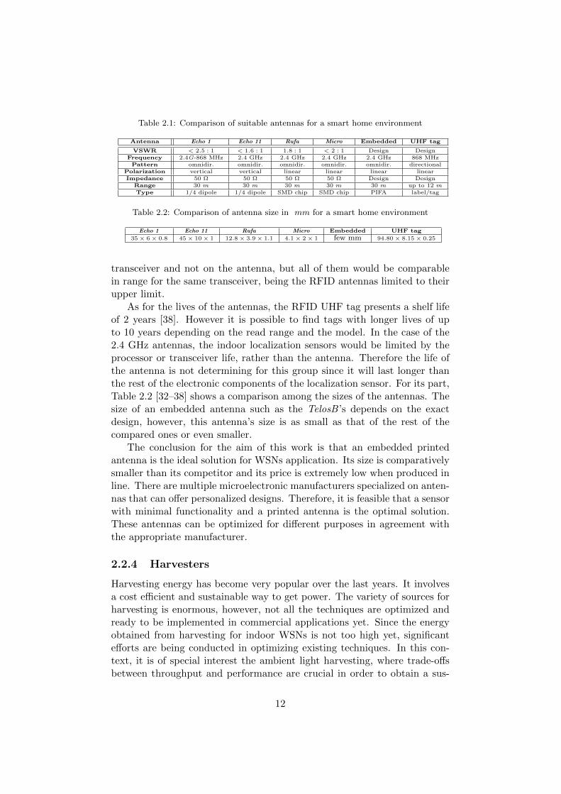
Table 2.1: Comparison of suitable antennas for a smart home environment

Antenna Echo 1 Echo 11 Rufa Micro Embedded UHF tag

VSWR < 2.5 : 1 < 1.6 : 1 1.8 : 1 < 2 : 1 Design DesignFrequency 2.4G-868 MHz 2.4 GHz 2.4 GHz 2.4 GHz 2.4 GHz 868 MHzPattern omnidir. omnidir. omnidir. omnidir. omnidir. directional

Polarization vertical vertical linear linear linear linearImpedance 50 Ω 50 Ω 50 Ω 50 Ω Design Design

Range 30 m 30 m 30 m 30 m 30 m up to 12 mType 1/4 dipole 1/4 dipole SMD chip SMD chip PIFA label/tag

Table 2.2: Comparison of antenna size in mm for a smart home environment

Echo 1 Echo 11 Rufa Micro Embedded UHF tag

35× 6× 0.8 45× 10× 1 12.8× 3.9× 1.1 4.1× 2× 1 few mm 94.80× 8.15× 0.25

transceiver and not on the antenna, but all of them would be comparablein range for the same transceiver, being the RFID antennas limited to theirupper limit.

As for the lives of the antennas, the RFID UHF tag presents a shelf lifeof 2 years [38]. However it is possible to find tags with longer lives of upto 10 years depending on the read range and the model. In the case of the2.4 GHz antennas, the indoor localization sensors would be limited by theprocessor or transceiver life, rather than the antenna. Therefore the life ofthe antenna is not determining for this group since it will last longer thanthe rest of the electronic components of the localization sensor. For its part,Table 2.2 [32–38] shows a comparison among the sizes of the antennas. Thesize of an embedded antenna such as the TelosB ’s depends on the exactdesign, however, this antenna’s size is as small as that of the rest of thecompared ones or even smaller.

The conclusion for the aim of this work is that an embedded printedantenna is the ideal solution for WSNs application. Its size is comparativelysmaller than its competitor and its price is extremely low when produced inline. There are multiple microelectronic manufacturers specialized on anten-nas that can offer personalized designs. Therefore, it is feasible that a sensorwith minimal functionality and a printed antenna is the optimal solution.These antennas can be optimized for different purposes in agreement withthe appropriate manufacturer.

2.2.4 Harvesters

Harvesting energy has become very popular over the last years. It involvesa cost efficient and sustainable way to get power. The variety of sources forharvesting is enormous, however, not all the techniques are optimized andready to be implemented in commercial applications yet. Since the energyobtained from harvesting for indoor WSNs is not too high yet, significantefforts are being conducted in optimizing existing techniques. In this con-text, it is of special interest the ambient light harvesting, where trade-offsbetween throughput and performance are crucial in order to obtain a sus-

12

tainable network [44].Notwithstanding, the most common sources of harvested energy that

could be applied in a smart home localization environment are the RF har-vesting and the solar harvesting. Whereas the RF harvesting is speciallyindicated for indoor, the solar harvesting could be used in the outer part ofa home, such as external walls, balconies or gardens. The size of the RFharvesters is still far from being optimal, whereas the solar harvesters offerbetter integration and space consumption. While the energy obtention andstorage efficiency techniques develops, it is interesting to consider these twocommercially available sources in order to foresee future trends.

RF harvesters. RF Harvesters use the electromagnetic energy available inthe ambience in order to feed a battery or capacitor where they storethe harvested energy. There is also a possibility of using no energystorage device and directly transmitting the collected energy to thetransceiver of the localization sensor. In the last case, the energyrequirements of the localiztion sensor should be minimum and theservice would not be guaranteed in all situations.

In order to feed a RF harvester, there are two techniques. The first oneconsists of using a powerful RF reader that sends an electromagneticsignal that is scattered throughout the indoor environment. This sig-nal feeds the harvesters that would provide the localization node withenergy or store for future use if they are provided with the appropri-ate device. An energy efficient approach could involve only activatingthe RF reader when an event occurs. The reader must however beconnected to the electric grid. On the other hand, if the existing elec-tromagnetic energy available in the ambience is enough in order tofeed the localization sensors, this energy can be used. This is not acommon situation in a smart home localization environment, since theavailable RF power in the air is not too high.

A representative commercial model of an RF harvester is the PowercastP2110 [45], which receives the RF power in the 850 MHz - 950 MHzband and is able to feed 2.4 GHz transceivers. The harvester can beused to feed a battery or, if the collected power is strong enough, todirectly provide a transceiver with power.

Solar harvesters. These devices use the power obtained from solar radia-tion in order to generate the power. There are several manufacturersof solar panels of various kinds. The panels should be adapted to theneeds of the specific sensor. Depending on the location of the har-vester, it can provide enough power for a localization sensor to work.Nevertheless, the availability of the power is a problem, since it de-pends on external factors. Storage devices are needed when the sunpower is not available.

13

Chapter 3

Modelling of the IndoorWireless Radio Channels

The interest in the ISM bands has progressively grown. These bands offerunlicensed operation meaning that no authorization needs to be issued, butit does not involve lack of regulation, since certain technical requirementsmust be followed. This section aims to study the propagation models for the865 MHz and 2.4 GHz bands, which are the most suitable for the design ofa localization network for smart homes. In order to characterize a channel,a first approach can be measuring its impulse response. A channel soundercan be used for this purpose [46].

Since the existing indoor propagation models are applicable to differentfrequencies, most of them can provide an estimation for both band ranges.That is the reason for why this chapter begins with an introduction toindoor propagation models that are analytically developed together with asemi-empirical approach and then proceeds to review the statistic analysisavailable for the more specific band ranges.

3.1 General Indoor Path Loss Propagation Models

Indoor environments differ significantly from outdoor environments in thatmultipath has a stronger influence and objects and movement have strongerconsequences on the propagation. This section presents the general ana-lytical semi-empirical methods for indoor. The models work for variousfrequencies and are therefore suitable for both of the frequency ranges thatwe are considering for the smart home environment.

14

3.1.1 The ITU Indoor Path Loss Model

The ITU model describes the loss [47–49] that a signal experiences in theradio link as

L = 20 log (f) +N log (d) + Lf (n)− 28 dB, (3.1)

whereN is the distance power loss coefficientf is the frequency in MHzd is the distance in meters (> 1)Lf (n) is the floor penetration loss factorn represents the number of floors between transmitter and receiver

ITU provides values for the factors in different environments and fre-quencies. This model takes into account the presence of objects and theeffects of the walls.

3.1.2 The Log-Distance Path Loss Model

This model describes the loss [47,49] as

L = B + 10A log (d/d0) dB (3.2)

B = PL(d0) +XσB (3.3)

Xσ ∼ N (0, σB) (3.4)

wherePL(d0) is the path loss at the reference distance d0 (normally 1 m)A is the Path Loss Exponent (PLE) which depends on the environment andtype of building that we are consideringXσB is a Gaussian random variable of mean 0 and standard deviation ofσB dB which models the shadow fading effects

The values for these parameters are also available in tables in order toadapt it to every environment and different frequencies. This model includesthe effects of shadow fading in its random variable.

3.1.3 Indoor Attenuation Factors

The various partitions that we can find in an indoor environment and theireffects on the attenuation can be merged in the following model: [50]

Pr dBm = Pt dBm− PL(d)−Nf∑i=1

FAFi −Np∑i=1

PAFi, (3.5)

15

wherePr and Pt are respectively the received and transmitted powersPL(d) is the path loss obtained analytically or experimentallyFAFi is the Floor Attenuation Factor for each floorPAFi is the Partition Attenuation Factor for each partition

The measurements for the partition and floor losses are available in var-ious sources.

3.1.4 Simplified Path Loss Model

This model aims to provide a more general view rather than focusing onprecise experimental studies for each case expressing the attenuation as [50]

Pr dBm = Pt dBm +K dB− 10A log (d/d0), (3.6)

wherePr and Pt are respectively the received and transmitted powersK depends on the antenna characteristics and channel attenuationA is the power decay index or PLEd0 is the reference distance

As noted by Goldsmith [50], K, A, and d0 can be obtained throughapproximations of existing models. Equivalently, the one-slope model canbe described as [51]

L = PL(d0) + 10A log (d) dB, (3.7)

wherePL(d0) is the path loss at d0 = 1 meterA is the PLEd is the distance

3.1.5 Motley-Keenan Model

According to this model, the loss can be described as [46,52]

L = PL(d0) + 10A log (d/d0) + Fwall + Ffloor dB, (3.8)

where, as noted by Molisch [46], Fwall and Ffloor are the attenuations ofrespectively the walls and floors encountered and depend on the material.

16

3.1.6 Multi-Wall-and-Floor

The multi-wall-and-floor model [53], takes into account penetration factorsmore accurately

L = PL(d0) + 10A log (d) +

I∑i=1

Kwi∑k=1

Lwik +

J∑j=1

Kfj∑k=1

Lfjk dB, (3.9)

whereLwik is the attenuation due to the kth wall type iLfjk is the attenuation due to the kth floor type jI and J are respectively the number of walls and floorsKwi and Kfj are respectively the number of traversed walls and floors of acertain category

3.1.7 Shadow Fading

In order to model the fading cause by shadowing, the log-normal shadowingmodel can be used, being the log-normal distribution that models ratiobetween the transmit and receive power [50,54,55]

p(ψ) =ξ√

2πσψdBψe−

(10 logψ−µψ dB)2

2σ2ψdB , ψ > 0, (3.10)

whereξ = 10/ ln 10µψdB

is the mean of ψdB = 10 logψ and σψdNits standard deviation

3.1.8 Other Indoor Path Loss Models

The Ericsson Multiple Breakpoint Model [47, 49, 56] can be used for esti-mation of the worst case attenuation in an indoor environment. For theirpart, the partition losses models [49] for one floor or between floors offer acompilation of data collected by different researchers about the attenuationcaused by the different partitions and obstacles found in buildings.

Additionally, the attenuation factor model [49, 57] describes the loss inan indoor environment for 915 MHz. The model was improved by the mea-surements of Devasirvatham [58].

3.2 General Indoor Fading Models

Fading occurs when various signals are being transmitted simultaneouslyinterfering and can be caused by shadowing, blockage and multipath [47].

17

Whereas the path loss models the effects of the channel on a high scale,the fading models the small scale effects [49]. There are various fadingmodels both for outdoor and indoor. This section focuses on the indoorfading models that could be applied to a smart home environment. Unlikethe previous case, fading models follow statistic patterns, since their exactcharacterization is inviable due to the high number of reflections involved.

The signal envelope of a multipath component is commonly modelledwith a Rayleigh distribution of variance σ2 [49, 50]

pZ(z) =2z

Pre(−z2/Pr) =

z

σ2e−z

2/(2σ2), z ≥ 0. (3.11)

However, if the line-of-sight component is fixed, the quadrature and in-phase components do not have a null mean and the signal envelope followsa Ricean distribution [49,50,59]

pZ(z) =z

σ2e−(z2+s2)

2σ2 I0

( zsσ2

), z ≥ 0, (3.12)

Finally a more complete distribution that adapts better to the real en-vironments is the Nakagami distribution [50, 60]. It is often more practicalto use alternative models that offer better performance for simulation andwill be described throughout this section. Goldsmith [50] also describes thefinite state Markov channel as an alternative for the modelling that offers asimpler outline. The approximation of such a model has been performed fora variety of environments, including indoor [61].

A further alternative is to use a channel sounder [46] in order to obtaininformation about the indoor environment that is going to be modelled. Thesounder emits radiofrequency radiation and analyzes the reflected signals inorder to model the impulse response of the indoor space. The disadvantageis that, despite their accuracy, the results cannot be generalized to the restof the environments.

3.2.1 Various Characteristics

Another option in order to characterize the channel in a small scale is toseparately measure the important factors that define the channel. This canbe done for every new indoor environment or use approximations based onthe results previously obtained.

An important factor is the power delay profile Ac(τ), which is the au-tocorrelation of the channel impulse response c(τ, t), when ∆t = 0 and rep-resents “the average power associated with a given multipath delay” [50].The average delay spread and the root mean square delay spread can bedefined [50]

µTm =

∫∞0 τAc(τ)dτ∫∞0 Ac(τ)dτ

, (3.13)

18

σTm =

√∫∞0 (τ − µTm)2Ac(τ)dτ∫∞

0 Ac(τ)dτ. (3.14)

Moreover, the mean excess delay can alternatively be used to describethe root mean square (rms) delay spread [49]

τ =

∑k

P (τk)τk∑k

P (τk). (3.15)

στ =

√τ2 − (τ)2 (3.16)

Finally, a last important parameter to characterize the channel is thecoherence bandwidth Bc, which is the “frequency where AC(∆f) ≈ 0 forall ∆f > Bc” [50], being AC(∆f) the Fourier transform of the power delayprofile

AC(∆f) =

∫ ∞−∞

Ac(τ)e−j2π∆fτdτ. (3.17)

3.2.2 Saleh and Valenzuela Indoor Statistical Model

The Saleh and Valenzuela model is specifically designed for indoor environ-ments and is based on clusters with multipath components that follow aPoisson distribution for their arrival [46,62], being the impulse response

h(τ) =L∑l=0

K∑k=0

ckl(τ)δ(τ − Tl − τkl), (3.18)

and the distribution of arrival of clusters and rays

p(Tl|Tl−1) = Λe−Λ(Tl−Tl−1), l > 0, (3.19)

p(τkl|τ(k−1),l) = λe−λ(τkl−τ(k−1),l), k > 0, (3.20)

where Tl is the arrival time of the first path of of the cluster l and τkl is thedelay of the kth path in the cluster l [46, 62]. Λ and λ are respectively thecluster and ray arrival rates.

3.2.3 ∆-K

Like the Saleh and Valenzuela model, the ∆-K model [63, 64] supposes thearrival or multipath components in clusters. There are two states whoserespective arrival rates are λ0(t) and Kλ0(t); the process is normally in thefirst state and switches for ∆ units of time to the second state, switchingback to the first if no new multipath components arrive [65]. With differentcombinations of ∆ and K, the model can be adjusted to different environ-ments.

19

3.2.4 Wide-Sense Stationary and Uncorrelated Scatterers

In order to simplify the correlation function, the wide-sense stationary as-sumption and the uncorrelated scatterers assumpation can be used [46] inorder to obtain the conditions that are easier to be fulfilled. If we representthe Wide-Sense Stationary and Uncorrelated Scatterers as a tapped delayline, the impulse response is [46]

h(t, τ) =N∑i=1

ci(t)δ(τ − τi), (3.21)

whereN is the number of tapsci(t) are the coefficients for the tapsτi is the delay for each tap

Molisch [46] describes further adaptations to the model supposing thatcertain conditions are fulfilled.

3.3 The 2.4 GHz Band

One of the most commonly used bands is the one that spans the range 2.4GHz - 2.4835 GHz, hereafter referred to as the 2.4 GHz band. The modelsthat have already been described are generally applicable to this range,however, this section presents specific results for it.

The 2.4 GHz band offers a broad spectrum range with relative unifica-tion concerning the standardization performed by the different bodies in thevarious countries and continents. This fact has implied that many manufac-turers and enterprises have chosen this band for the operation of a varietyof devices that do not need to operate in a licensed band. Microwave ovensand standards such as WiFi or Bluetooth are examples of operation in thisband, where the WSNs have also been developed. The agency in charge ofthe standardization of the WSNs in Europe is the European Telecommu-nications Standards Institute (ETSI) in its European TelecommunicationsStandard (ETS) 300 328 [66], where the equipment and transmission systemsare harmonized. For its part, it is the Federal Communications Commis-sion [67] that rules the ISM bands including the 2.4 GHz band in the UnitedStates.

3.3.1 Path Loss Models’ Results in the 2.4 GHz Band

All the proposed path loss models include verification stages where theiraccuracy has been tested prior to their validation. However, this sectionpresents additional external results on path loss focusing on the 2.4 GHzband.

20

Souza et al. proposed a new model for 2.4 GHz and performed a com-parative analysis of various models, including the ITU model and the log-distance model in [68], finding root mean square deviation errors between 3and 8 dB for these models and confirming their validity for this frequencyband. An additional comparative analysis between the ITU, the one-slope,and the multi wall models in a smart home environment can be found in [69],showing that the multi wall model is the most accurate, and that the ITUmodel can be adjusted with the information gathered by the one-slope modelin order to increase its accuracy.

For its part, a comprehensive analysis of the multipath parameters forvarious frequencies has been conducted in [70], which studies the path lossfor 2.4 GHz. Writing the loss as

L = PL(d0) + 10A log (d) + b, (3.22)

the values found for A and b in [70] at 2.4 GHz were respectively between1.86 and 3.33, and −1.6 and −5.4 dB, being the rms error σL = 1.6-3.6 dB.Moreover, with people inside the room, the attenuation variation was foundto be between −0.33 and 4.84 dB depending on the antenna height and theline of sight [70].

Alternatively, the linear attenuation expressed following the model [58]

L = PL(d0) + 10A log (d) + ad dB, (3.23)

was analyzed in [71], finding for a smart home environment, values of A = 1.8and a = 2.25-6.11 dB/m depending on whether it is a same floor or amultifloor scheme. Further experimental results from the 2.4 GHz bandare shown in [72], where the log-distance path loss model, the log-normalshadowing, and fading effects are characterized and presented for an indoorenvironment.

In [73], the one-slope, and multi wall models are evaluated for 2.4 GHz;after simulations in software and subsequent testing of their accuracy in thereal environment, the multi-wall models were found to offer better accuracy,being the mean error around 5.5 dB for the linear and one-slope models and4 dB for multi wall, whereas the standard deviation was around 4 dB forthe linear and one-slope models and 2.8 dB for the multi wall ones.

Finally, the research conducted in [74] found that the texture of thesurfaces and the presence of small objects influences significantly the es-timations. These are, however, not possible to predict unless the indoorenvironment is known beforehand. A new propagation model based on em-pirical measurements is proposed in [75] and tested with the IEEE 802.15.4standard for localization, showing better performance than other existingmodels. Finally, the Matrix Pencil algorithm has provided a successful su-perresolution approach [76].

21

3.3.2 Fading Models’ Results in the 2.4 GHz Band

The basic parameters for the small scale modelling of the channel, the meandelay spreads τrms has been found to range between 5.4 and 23.1 ns at 2.4GHz depending on the presence of people, the line of sight and the antennaheights [70]. Regarding the rms delay spread στrms standard deviation, ithas been found to range between 0.5-17.0 ns at 2.4 GHz [70]. For its part,the coherence bandwidth has been found to range around 250 MHz in lineof sight and much less in obstructed direct path [70]. Finally, the powerdelay profile has been found to range between −90 and −65 dB, with peaksof −105 dB between 0-250 MHz at 2.4 GHz [70].

Complementary results concerning these parameters can be found in[77], where several measurements in different indoor environments (gym,office, etc.) were performed, obtaining mean delay spreads τrms between12 and 43ns and rms delay spreads στrms between 45 and 420ns dependingon the location; the coherence bandwidth was for its part between 3-55MHz. Further research conducted in [78] has provided values of the meandelay spread τrms between 43 and 57ns, rms delay spread στrms between22 and 30ns, and coherence bandwidths between 654-901 kHz (with olderequipment).

For its part, a comprehensive research is conducted on shadowing in [79]validating again the accuracy of the multi wall model with errors between0% and 5%. The shadowing deviation calculated and applicable to the log-distance path loss model was found to be between σ = 0-21.97 dB dependingon no floor to two floors differences [79]. Further research on fading hasdetermined the Ricean k = z2

max/(2σ2) factor between 1.3 and 8.7, and

the rate of crossings of envelope levels from 6 to 12 dB between 3.183 and0.051 s−1 [80].

As for the Saleh-Valenzuela and ∆-K models, their performance wasanalyzed (in ultra wideband) in [81], resulting in Λ = 0.0223 ns−1, λ =2.5 ns−1. Substantial differences were found between two models, beingthe Saleh-Valenzuela more accurate and the clustered arrival of multipathcomponents was confirmed for most cases [81].

3.4 The UHF Band

The UHF range also belongs to the ISM bands, inheriting all the benefitsof being unlicensed. This band, however, presents more problems as far asagreement on the unlicensed ranges among the various agencies throughoutthe world. Whereas in Europe the 865-868 MHz band is unlicensed andcommonly used for WSNs and RFID, in America it is the 902-928 MHzband that is not subject to licensing [1]. This can create multiple problemswith standards when commercial products are launched. Comparatively, theUHF band presents a narrower bandwidth than the previously described 2.4

22

GHz band, but has been on the other hand less intensively used so far.However, RFID has found in this band a useful range of frequencies todevelop passive tags, described in Chapter 2. This section analyzes thefindings on both the European and American ranges for the UHF band.

3.4.1 Path Loss Models’ Results in the UHF Band

Analogously, the general path loss models that have been published includetesting batteries to certify their validity. This section aims however to pro-vide data on research that has been particularly conducted on the UHFband.

It has been shown [82] that for a linear model expressing the loss as

Pr = P − 10A log (d), (3.24)

the value of A ranges between 2 and 3. Complementary studies on path losshave shown n ranging from 2 to 5 in various indoor locations [57], confirmingthe validity of the results. As for the Floor Attenuation Factor (FAF), ithas been found to range between 12 and 30 dB. Furthermore, Cheung et al.present a new model for indoor propagation prediction in [83], where theconventional path loss models errors are also analyzed at UHF, resulting ina mean error of 14.8 dB, and a deviation error σ of 20.8 dB.

3.4.2 Fading Models’ Results in the UHF Band

The mean delay spread τrms has been found to be between 24 and 28 ns, rmsdelay spread στrms between 4.5 and 6 ns, and coherence bandwidths between5.35-8 MHz [82]. Further research on rms delay spread at UHF can be foundin [84], where this parameter is analyzed in a variety of indoor environmentswith multiple walls and floors, resulting in values between 20 and 250 nsdepending on the exact environment.

As for the Nakagami and Ricean k factor, it has been found to rangebetween −5.2 and 36.7 dB depending on the line of sight and the particularindoor distribution [85]. For its part, the log-normal distribution has beenfound the best candidate to model RFID tags for multiple indoor environ-ments at UHF bands [86].

3.5 Comparison between the Bands

The empirical results obtained in the various measurements described alongthis chapter show that both the 2.4 GHz band and the UHF band presentsimilar features and characteristics. The 2.4 GHz band presents broaderbandwidth to deploy systems and applications, but offers a more intensively

23

used environment where more devices are normally operating. Notwith-standing, the techniques against interference are more refined in the 2.4GHz band.

The comparison between both bands performed in this chapter is sup-ported by the data collected in [87], where large and small-effects’ parame-ters prove to be comparable in both ranges. Finally, a detailed comparison isconducted in [88], stating the lower noise in the UHF band due to the smalleramount of applications and the smaller bandwidth as well as the problemswith the variations in performance that the UHF on the other hand poses.For the scope of this work, both bands are suitable and it should be otherfactors, such as the best available hardware, that will affect the election.

24

Chapter 4

Overview on Estimation andLocalization Techniques

This chapter aims to provide an overview on the estimation theory thatcan be applied in order to make a decision on the characteristics of thereceived signal. Interesting research in this area can be found in [89–91]. Thealternative models that can be considered in order to estimate an unknownreceived parameter are presented here. The idea is to estimate an unknownparameter that can be corrupted by noise by measuring a received signal thatmay also be noisy. All the models described throughout this chapter havealternative representation under the assumption of a linear model, which isdeveloped in [92].

4.1 Classical Estimation

The classical estimators are based on the idea that the unknown parametersto be observed and estimated are deterministic [92]. This section providesan insight into the most common classical estimators.

4.1.1 Best Linear Unbiased Estimator

One of the most commonly used classical estimator is the Best Linear Un-biased Estimator (BLUE), based on the Gauss-Markov theorem, which cal-culates the estimation θ of the p× 1 vector θ from the received data x withcovariance matrix C as [92]

θ = (HTC−1H)−1HTC−1x, (4.1)

where x = Hθ+w, where is H an n×n known matrix, and w a noise vectorof zero mean and covariance matrix Cw = C, under the assumption that theexpected value E[x] = Hθ.

25

4.1.2 Least Squares Estimator

Another useful estimator is the Least Squares Estimator (LSE), which esti-mates θ as the value of θ that minimizes the function [92]

J(θ) = (x− (s(θ))T (x− s(θ)) =N−1∑n=0

(x[n]− s[n; θ])2, (4.2)

where x[n] = s(n; θ) + w[n], n = 0, 1, . . . N − 1, where s is a known signal.

4.1.3 Other Classical Estimators

A third classical estimator is the Maximum Likelihood Estimator (MLE),which assumes that the estimated value θ is obtained as the value θ that min-imizes the Probability Density Function (PDF) f(x; θ), which is supposedto be known [92]. Additional classical estimators are the Rao-Blackwell-Lehmann-Scheffe, and the method of moment estimator, whose descriptioncan be found in [92].

4.2 Bayesian Estimation

The Bayesian estimation differs from the classical approach in that the pa-rameter θ to be estimated is not deterministic, but a random variable ofwhich a realization will be estimated [92]. This section provides an overviewon the most common Bayesian estimators.

4.2.1 Minimum Mean Square Error

One of the most popular estimators of this kind is the Minimum MeanSquare Error (MMSE) Estimator, where the estimation θ = E[θ|x], wherethe expectation with respect to the PDF is [92]

f(θ|x) =f(x|θ)f(θ)∫f(x|θ)f(θ)dθ

. (4.3)

A particular case is x and θ being jointly Gaussian, then θ = E[θ] +CθxC

−1xx (x − E[x]) [92]. Finally, the Bayesian Mean Square Error (MSE)

is defined as [92]

Bmse(θi) = E[(θi − θi)2

](4.4)

4.2.2 Kalman Filter

The Kalman filter is a particular case of linear MMSE. However, due toits importance, it is described separately in this subsection. In its scalardefinition, for n ≥ 0, the prediction is described [92,93]

s[n|n− 1] = as[n− 1|n− 1], (4.5)

26

where s[n|n − 1] denotes the prediction of s in time n based on all theprevious measurements. For its part, the minimum prediction MSE [92,93]

M [n|n− 1] = a2M [n− 1|n− 1] + σ2u, (4.6)

where σ2u the variance of the driving noise, and a the filter parameter. The

Kalman Gain is [92,93]

K[n] =M [n|n− 1]

σ2n +M [n|n− 1]

, (4.7)

where σ2n is the variance of the noise w[n] from the observation ecuation

x[n] = s[n] + w[n]. Finally, the minimum MSE is calculated [92,93]

M [n|n] = (1−K[n])M [n|n− 1]. (4.8)

The results are easily translated to a vector definition and there areextensions of the filter described in [92]. The Kalman filter has been exten-sively used in estimation for WSNs.

4.3 Cramer-Rao bound

The Cramer-Rao bound defines the lower bound of the goodness of theestimation of an unknown parameter given a number of observations andnoise and it is given, in its form for a deterministic parameter, by [94]

Var[θ(x)− θ] ≥−E

[∂2

∂θ2ln f(x|θ)

]−1

. (4.9)

In its form for a random parameter, the lower bound is [94]

E[(θ(x)− θ)2

]≥

E[∂∂θ ln f(x|θ)2

]−1

=−E

[∂2

∂θ2 ln f(x|θ)]−1 (4.10)

4.4 Channel Model Parameters Estimation and Lo-calization

The environments where WSNs will work are normally not known before-hand. It is important to be able to estimate the parameters of the wirelesschannel where the WSNs is going to operate. A possible approach is toperform an initial stage with various measurements knowing the nodes lo-cation in order to calibrate the channel propagation parameters and adaptthem to the working environment. Alternative approaches are estimatingthe channel model parameters and the unknown location of target nodes

27

by analyzing the received power, knowing only the location of some anchornodes. This section describes both the approach of only estimating thechannel parameters, which could allow to estimate the distance in a furtherstep, once they are known, and the approach of estimating the location andchannel parameters together.

4.4.1 Channel Parameters Estimation

This section presents the existing methods for the estimation of the pa-rameters of the wireless channel. The distance is not estimated throughthis methodologies, though it can certainly be estimated subsequently byapplying the known propagation models.

Method 1.1

This method, proposed in [95], enables us to estimate the path loss parame-ters in any point of an indoor environment by using the measurements froma node that knows its distance and path loss to three anchor nodes. It pro-vides two approaches, a non-parametric and a optimum linear estimationalgorithm (provided that the path loss parameters are known). The methoduses the path loss model [54,96]:

L(dB) = B + 10A log(d/d0) d ≥ d0, (4.11)

B = PL(d0) +XσB , (4.12)

XσB ∼ N (0, σB) (4.13)

where B and A are respectively the path loss intercept and path loss ex-ponent, d0 is assumed to be 1 meter as it is common [49], and XσB is azero mean Gaussian random variable of standard deviation σB (dB) and itsspatial variability is characterized in [95].

The non-parametric approach is described here [95]; 1)the node thatwants to localize a point in the room measures the path losses to the threeanchor nodes L1, L2, L3; 2)let the functional approximations be L′i = B′ +10A′ log (di) for i = 1, 2, 3 and using LSE find B′ and A′ that minimizethe mean square difference between Li and L′i; 3)calculate ∆i = Li − B′ −10A′ log (di); 4)calculate for the unknown point to be localized ∆0 = k1∆1 +k2∆2 + k3∆3, where

ki =d−ν0i

d−ν01 + d−ν02 + d−ν03

,

where di are the distances from the node that wants to localize a point inthe room to the anchor nodes, and ν is taken 1 in [95] after measurementsthat show the differences in error to be small; finally, 5)estimate the pathloss to the unknown point L0e = B′ + 10A′ log (d0) + ∆0.

28

The optimum linear estimation approach [95] assumes that A and α areknown and calculates the shadow fadings si = Li−PL(d0)−10A log (di/d0);then s0 can be estimated s0e = a1s1 + a2s2 + a3s3. The expressions for aican be found in [95].

Method 1.2

This method is proposed in [97] and uses linear-square-fitting. It consistsof 1)various anchor nodes whose position is known that receive packets ina scheduled way, 2)estimation of the RSS indicator between anchor nodes,3)computation of the distance between anchor nodes, 4)local computationof the 2 channel parameters via linear square fitting, 5)sending of the pa-rameters to the nodes whose position is unknown [97].

Method 1.3

This method, described in [98, 99], enables us to estimate the PLE by onlyusing measurements of the received power and the planarity geometric con-straints, without needing to rely on distance measurements. It offers threescenarios: estimation based on the probability distribution of distancesamong sensors being known, more general estimation using only the re-ceived power and the geometric constraints based on the Cayley-Mengerdeterminant, and a last one based on pattern matching. This method usesthe commonly employed log-normal model of the form [49,98]

Pij [dBm] ∼ N (Pij [dBm], σ2dB), (4.14)

Pij [dBm] = P0(d0)[dBm]− 10A log(dij), (4.15)

where the reference power at distance d0 (commonly taken as 1 meter forindoor [49]), P0(d0), is assumed to be known from a priori calibration.Moreover, the power is supposed to be symmetrically distributed betweenboth nodes Pij = Pji, noting that the average value could be taken if it wereasymmetric. For its part, α is the PLE. The variance of the shadowing σ2

dB

does not need to be known either for the application of this model.The first approach, supposing a known node-distance probability distri-

bution, enables us to obtain α by solving the equation [98]

E(Pij [dBm]) =

∫ b

aP0[dBm]− 10A log (x)dx = E(Pr), (4.16)

where E(Pr) is the sample mean of the received power. Alternatively, ifthe transmitter power is known, a more general estimate of A comes fromminimizing the function f(A), based on a set of quantile points uniformly

29

distributed whose distances di are known, since this is a hypothesis in thisfirst approach [98]

f(A) =

N∑i=1

(Pi[dBm]− P0[dBm]), (4.17)

A =

−N∑i=1

(Pi[dBm]− P0[dBm]) log di

N∑i=1

10(log di)2

(4.18)

A second approach does not require knowledge of the distance probabilitydistribution, only the received power and geometrical constraints; it uses theMLE to obtain the likelihood function of a quadrilateral of sensors that willconstitute the four anchor nodes [98]:

L(d12, d13, d14, d23, d24, d34, A) =

=1

(√

2πσdB)6

∏1≤i<j≤4

exp

(−(Pij − P0 + 10A log(dij))

2

σ2dB

)(4.19)

After mathematical development of this equation and using the Cayley-Menger determinant [100,101], A can be obtained by numerically solving [98]

h(A) =

∣∣∣∣∣∣∣∣∣∣∣

0 C−2/A12 C

−2/A13 C

−2/A14 1

C−2/A12 0 C

−2/A23 C

−2/A24 1

C−2/A13 C

−2/A23 0 C

−2/A34 1

C−2/A14 C

−2/A24 C

−2/A34 0 1

1 1 1 1 0

∣∣∣∣∣∣∣∣∣∣∣= 0, (4.20)

where Cij = Pij/P0, 1 ≤ i < j ≤ 4 are known. It is important to remarkthat this method presents a high bias [98].

Finally, a third approach is proposed in [98] in order to correct the bias ofthe second one, based on pattern matching for various quadrilaterals withinthe WSNs; σ2

dB,j+1 − σ2dB,j = ∆σ2

dB, and Ai+1 − Ai = ∆A. The algorithmthat must be followed involves [98]: 1) identify a set of quadrilaterals in thenetwork, 2) add Gaussian noise with variance ∆σ2

dB into the measurement, 3)

for each quadrilateral solve A with the second approach used above and aver-age E(A)1, repeat 2) and 3) using M∆σ2

dB,M = 0, 1, . . . ,m where M = 0 is

the original data set, obtaining (0,E(A0)), (∆σ2dB,E(A1)), . . . , (m∆σ2

dB,E(Am)),find values of i and j in a database such that

i, j = arg mini,j

m∑N=0

(E(A)N − E(A)Ai,σ2dB,j+N

)2, (4.21)

30

(m ≥ 500), and 6)once obtained i and j, improved estimates are A = Aiand σdB = σdB,j .

This last technique can be improved using data fusion, denoting theestimate from σA (instead of E(A)), σdB, and A by σs and the estimate

from E(A), σdB, and A by σb, ~A = [AsAb]T , the new estimation using fusion

techniques is A = W T ~A [98], where W = C−1DT (DC−1DT )−1 [102], where

C = E

[As −AAb −A

] [As −AAb −A

]T, D =

[1 1

].

Method 1.4

This method is proposed in [103] and aimed at homogeneous planar Poissonpoint distributed nodes, considering Nakagami-m fading and interference.The method also describes three different algorithms. It does not require toknow the location of the nodes.

The first technique assumes a known distribution density of the nodesand uses the mean value of the interference [103]. The mean received poweris µR = µI +N0 [103], where N0 is the Additive White Gaussian noise meanpower and

µI = 2πλpR2−A

0

A− 2,

is the mean theoretical interference [104], where R0 the near-field radius ofthe antenna, p is the ALOHA contention probability, λ is the node distribu-tion density, and A is the PLE. The algorithm then saves the received powersR1, . . . , RN , whose mean converges, during an N interval, and equates µRto the observed mean value in order to obtain A through a look-up tableand the rest known parameters.

The second technique does not require knowledge of the Nakagami pa-rameter or the node distribution density. The Signal to Interference plusNoise Ratio (SINR) is required, but the nodes can virtually compute itas if the received powers were realizations of an exponential random vari-able [103]. Therefore, the nodes should record the powers R1, . . . , RN andtake the signal powers Si as realizations and obtain the corresponding SINR,then evaluate the success probability in the Poisson network ps at two SINRthresholds Θj [103]

ps,j =1

N

N∑i=1

1Si/Ri>Θj , j = 1, 2,

where 1 is added when the condition Si/Ri > Θj is met. The estimate canbe proved to be [103]

A =2 ln(Θ1/Θ2)

ln((ln ps,1 +N0Θ2)/(ln ps,2 +N0Θ2)), (4.22)

31

independently from λ and m.Finally, the third algorithm is based on the proposition that the trans-

mitting set of a node (“group of transmitting nodes whom it receives apacket from”), namely NT , is proportional to Θ−2/A if m ∈ N and N0 I[103]. The the algorithm is as it follows [103]: 1)for a known Θ1 ≥ 1, setNT,1(i) = 1, at time slot 1 ≤ i ≤ N if the node can decode a packet or 0otherwise, the mean NT,1 will converge, 2)proceed analogously with NT,2,3)the estimation can be proved to be

A =2 ln(Θ2/Θ1)

ln(NT,1/NT,2). (4.23)

As noted by the authors of the method [103], this algorithm is also biased,though measures are proposed to address it.

4.4.2 Joint Channel Parameters and Distance Estimation

This subsection reviews the existing methods that allow an estimation ofthe parameters and the distance. The results are presented below.

Method 2.1

This method offers a non linear least square estimation. Described in [105],it notes the equation

PLi = gi(θ) +B, 1 ≤ i ≤ n, (4.24)

where PLi = P0 − Pri is the path loss observation, being P0 known; gi(θ) =10A log (di); θ = [θ1, θ2, θ3]T = [x, y,A]T ; and B ∼ N (0, σ2

B) due to shadowfading. This leads to the vector form P = g(θ) +B, where the componentsare P = [PL1 , . . . 0, PLn ]T ; g(θ) = [g1(θ), . . . 0, gn(θ)]T ; B = [B1, . . . , Bn]T

[105]. Thus, the function ξ(θ) = (p−g(θ))T (p−g(θ)) needs to be minimized,and by applying a Taylor expansion to g(θ) and using the Jacobian matrix,the solution is [92,105]

θ = θ(0) + ((J (0))TJ (0))−1(J (0))T (p− g(θ(0))), (4.25)

where

[J (0)]ij =∂gi(θ)

∂θj

∣∣∣∣θ=θ(0)

.

As noted by the authors of the algorithm [105], a further improvement canbe done to reduce the error by using the Gauss-Newton algorithm.

32

Method 2.2

This method, proposed in [106], uses a propagation model such as

P (d) = bd−a (mw), (4.26)

where in this occasion b is the channel constant attenuation and a is the PLEin linear format. The PDF p(P |d, b, a) is defined, where P = [P 1

11, . . . , PNOM ],

being P kij the kth received power at the jth anchor node from the ith targetnode; for their part O is the number of target nodes and d = [d11, . . . , dOM ]are the distances dij between the ith target node and the jth anchor node[106]

dij =√

(Xi − xj)2 + (Yi − yj)2 + (Zi − zj)2, (4.27)

where Zi is assumed to be known for simplicity, though it is easily transpos-able to three dimensions. If P kij are independent, then [106]

p(P |d, b, a) =

O∏i=1

M∏j=1

N∏k=1

p(P kij |dij , b, a), (4.28)

p(P kij |dij , b, a) =1

bd−aijexp

(−P kij

bd−aij

), (4.29)

and the log-likelihood function is L(d, b, a) = ln p(P |d, b, a) [106]. Then,the algorithm proceeds with two stages. In the first one, the locationsXn = [X1, . . . , XO] and Yn = [Y1, . . . , YO], where n is the iteration cy-cle, are estimated to then obtain the estimates Xn, Yn by maximizing thelog-likelihood function of the first stage L1(dn, bn−1, an−1) [106]:[

∂L1(dn, bn−1, an−1)

∂Xi

]Xi=Xi

=

=

O∑i

∂

∂Xi

M∑j

N

ln

(1

bn−1d−an−1

ijn

)−∑N

k Pkij/N

bn−1d−an−1

ijn

Xi=Xi

= 0, (4.30)

and analogously for Yi = Yi.Once obtained the target node locations Xn, Yn and the distance dn, in

the second stage, the ML estimates bn, an are obtained by maximizing thelog-likelihood function L2(dn, bn, an) with respect to bn and an [106]:[

∂L2(dn, bn, an)

∂bn

]bn=bn

=

=

∂

∂bn

O∑i

M∑j

N

ln

(1

bnd−anijn

)−∑N

k Pkij/N

bnd−anijn

bn=bn

= 0, (4.31)

33

and analogously for an = an. Then further iterations take place until |bn −bn−1| <tolerance b and |an − an−1| <tolerance a [106].

Method 2.3

This method, described in [107], is based on a particle filter [108] and it aimsto recursively obtain the PDF p(si(t)|z(t), where si(t) = xi, yi, Ai1, . . . , AiKis the state of the ith particle being xi, yi the coordinates, Aij the estimatedpath loss exponents of the log-normal model, and z(t) the observation. Fur-thermore, a weight wi(t) is associated to the samples in t− 1 [107,109].

The algorithm begins with a prediction where the parameters can onlyvary between ALOS = 1.8 and ANLOS = 0 [107]:

xi(t) = xi(t− 1) + nx∆t

yi(t) = yi(t− 1) + ny∆t

Aij(t) =

ALOS if (nn ≤ pchange&&nij(t− 1) == ANLOS)

ANLOS if (nn ≤ pchange&&nij(t− 1) == ALOS) ,

where nx ∼ N (0, σposition), ny ∼ N (0, σposition), nn ∼ U(0, 1), ∆t is theinterval between iterations. Then, in a second stage, the update is [107]

wi(t) = wi(t− 1)p(z(t)|xi(t))

wi(t) =wi(t)∑Npj=1wj(t)

,

where Np is the number of particles of the filter. The expression for the jth

node is [107]

p(zj(t)|si(t)) =1

σL√

(2π)exp

(−

(zj(t)− PL,ij(d))2

2σ2L

), (4.32)

and

PL,ij(d)[dB] = PL(d0) + 10Aij log

(d

d0

),

which for the K anchor nodes results

p(z(t)|si(t)) =K∏j=1

p(zj(t)|si(t)). (4.33)

If an effective number of samples Neff = 1/(∑Np

i=1(wi(t))2) < Nthreshold,

resampling is performed [107]. Finally, the estimations can be computedas [107]

x(t) =

Np∑i=1

wi(t)xi(t)

34

y(t) =

Np∑i=1

wi(t)yi(t)

Aj(t) =

Np∑i=1

wi(t)Aij(t), j = 1, . . . ,K.

Method 2.4

This method, described in [110], describes the received power as P = CA+N , where C = diag([−10 log (d1), . . . ,−10 log (dn)]T );A = [A1, . . . , AN ]T isthe path loss exponent and N = [N1, . . . , NN ]T is the vector of uncertainties,being N the number of beacons. The distances d = [d1, . . . , dN ]T and pN ∝exp−(p−CA)TQ−1(p−CA)/2, being Q the diagonal covariance matrix,and (p− CA)T the estimation error vector, being C and A unknown [110].Using the Newton-Raphson method [110,111]

Ak = Ak−1 −∇Af(A)H(A)−1, (4.34)

where H(A) = 2CTQ−1C and ∇Af(A) = −2(p − CA)TCTQ−1 are theHessian and the gradient of f . The algorithm makes 1)initialization of α0,2)update C; for k ≥ 1 uses the estimates Ak−1 to compute C, 3)update Awith C, 4)alternate steps 2) and 3) [110]. The path loss estimation error atthe sensor i is ∆A

i = Aei −Ai, being Aei the estimated path loss factor [110].

35

Chapter 5

Localization Algorithm

This chapter describes the various approaches to improve the existing solu-tions. There are two main approaches: considering different path losses dueto shadow fading or considering a common path loss general to all pathsacting as a ‘balancing parameter.’

5.1 Analyzing the Path Losses separately

There are various approaches that can be followed if the localization is basedon considering different path losses. The problem that arises is that we findmore unknowns than equations, which leads to the problem behaving as anidentity in many cases or losing accuracy. However, these methods providea good mechanism of discovering Non Line of Sight (NLOS) paths that canbe discarded when using alternative methods, such as Time Difference ofArrival (TDOA), which are not considered as an option in this work due totheir high synchronization requirements.

The problem that we want to address considers this equation:

PLi = Bi +A10 log(di) + vi, (5.1)

where the path loss at distance d0, namely PL0, is included in Bi. Theshadow fading and noise vi are modelled as

Bi ∼ N (µB, σB); vi ∼ N (0, σn). (5.2)

The following subsections present different alternatives to approach thisproblem. The challenging part of this modelling is that both Bi and dineed to be estimated simultaneously.

5.1.1 Minimum Variance Unbiased Estimator

The minimum variance estimator can often not be obtained, due to its prac-tical difficulty when dealing with non linear systems [92]. A common ap-proach is to work with a linear version of the system, for which a standard

36

minimum variance estimator can be found. In order to obtain the minimumvariance estimator, the problem is expressed linearly in the form

P = Hθ + V, (5.3)

where P is the vector of measured losses, θ = [B1, . . . , BN , A] is the vectorof unknowns, V is the vector of shadow fading, and H is a known matrixthat defines the channel.

The minimum variance estimator θ = [B1, . . . , BN , A] of this problemis [92]

θ = (HTH)−1HTP. (5.4)

In order to solve this equation, the distances di need to be either anunknown in the vector θ or known and then be included in the matrix H.Both cases are disclosed below supposing 4 anchor nodes for simplicity:

• di known: If we suppose the distances di to the target node can beknown by other methods, then the matrix H is

H =

1 0 0 0 10 log(d1)0 1 0 0 10 log(d2)0 0 1 0 10 log(d3)0 0 0 1 10 log(d4)

,

which implies that

det (HTH) = 0 ⇒ @(HTH)−1 ⇒ @θ,

• di unknown: In this case, the distances are included in the θ =[B1, . . . , B4, A10 log(d1), . . . , A10 log(d4)] vector and the matrix H is

H =

1 0 0 0 1 0 0 00 1 0 0 0 1 0 00 0 1 0 0 0 1 00 0 0 1 0 0 0 1

,

once again

det (HTH) = 0 ⇒ @(HTH)−1 ⇒ @θ,

It can be observed that in both cases the minimum variance unbiased estima-tor does not exist. A final approach is to consider A and di known by othermethods. A can be known via one of the methods described in section 4.4whereas di could be known via an alternative method that provides a roughestimation. The idea here is to find an iterative method that progressivelyimproves the accuracy. In this case, the term A log(di) is moved to the Pvector, which includes now certain error that depends on the goodness of

37

the rough estimate of A and di. The equations that describe the systemresult now

P = Hθ + V, (5.5)

where P includes A log(di) and the possible error derived from it plus thepath loss measurements and H is

H =

1 0 0 00 1 0 00 0 1 00 0 0 1

. (5.6)

The system behaves now as an identity, which completely depends on theinitial guess of di. As an identity, the system will estimate Bi such thatthe equations are satisfied to fit the initially provided rough di. It will notimprove the performance and it will not be possible to use it in an iterativemethod, since in the best case it will maintain the error, but never decreaseit.

Finally, we can consider that:

• di are known by using another method and that

• Bi = B ∀i.

In this case

H =

1 10 log(d1)1 10 log(d2)1 10 log(d3)1 10 log(d4)

,

and a solution θ exists. However, the solution θ does not really improve thevariance of the existing methods described in section 4.4. An improvement tothe minimum variance estimator is proposed in [112], where a correction tothe minimum variance estimation θ is proposed provided that the covariancematrix C = σ(HTH)−1 is known and that θ : ||θ||2 ≤ θ2

0, where θ0 is known.Noting θb as the new biased estimator and θu the former unbiased estimator,the new estimator would be [112]

θb =θ2

0

θ20 + Tr((HTC−1H)−1)

θu. (5.7)

However, the problems previously described in this section are inherited andit is thus not possible to apply this improvement.

It can be observed that the bias bBi in this kind of approaches mainlydepends on the relative position of the anchor and unknown nodes

bBi = f(x, y, xi, yi). (5.8)

38

0

20

40

60

80

100

120

0

20

40

60

80

100

120−20

−10

0

10

20

30

40

50

60

xy

biasB

6

Figure 5.1: Relative bias in % of the path loss with the sixth anchor node B6 in theminimum variance estimator depending on the coordinates of the unknown node, measuredin decimeters. The peak corresponds to the coordinates of the anchor node 6. Similarfigures can be obtained for each anchor node. A clear dependence with the coordinatescan be observed.

An example of this can be observed in Figure 5.1, which is taken from aMatlab simulation with eight anchor nodes.

The alternative approaches that will be described in section 5.2 assume acommon Bi = B balancing the errors of the different paths and offer betterresults.

5.1.2 Minimum Mean Square Estimator

In the case of a MMSE estimator, it is possible to find a non linear esti-mator that adapts to our purpose, enabling us to estimate Bi, A, and thecoordinates (x, y). In order to adapt the MMSE estimator to our problem,a Kalman filter needs to be implemented; the model as presented in [92]consists of:

39

Prediction:

s[n|n− 1] = a(s[n− 1|n− 1]) (5.9)

Minimum Prediction Matrix:

M [n|n− 1] = A[n− 1]M [n− 1|n− 1]AT [n− 1] +BQBT (5.10)

Kalman gain Matrix:

K[n] = M [n|n− 1]HT [n](C[n] +H[n]M [n|n− 1]HT [n])−1 (5.11)

Correction:

s[n|n] = s[n|n− 1] +K[n](x[n]− h(s[n|n− 1])) (5.12)

Minimum MSE Matrix:

M [n|n] = (I −K[n]H[n])M [n|n− 1], (5.13)

where:s = [B1, . . . , BN , A, x, y], and s is the estimation of sa(·) and h(·) are functions that need to be adjusted to the problems[n] = a(s[n− 1]) +Bu[n]x[n] = h(s[n]) + w[n],where w[n] is the noise ni

A[n− 1] = ∂a∂s[n−1]

∣∣∣∣s[n−1]=s[n−1|n−1]

H[n] = ∂h∂s[n]

∣∣∣∣s[n]=s[n|n−1]

C and Q are the covariance matrices of the shadow fading and the noise.

Adapting the theory to our problem, we must consider that our un-knowns are not evolving with time. Therefore, even though the extendedKalman Filter allows time evolving systems, we will define the functions insuch a way that the system is static. Supposing for simplicity an unknownnode of coordinates (x, y) in the plane (although it can easily be extended tothree dimensions) and 8 anchor nodes whose known coordinates are (xi, yi),the algorithm for our problem is

a(s[n]) = s[n] (5.14)

h(s[n]) =

B1 +A10 log(√

(x− x1)2 + (y − y1)2)...

B8 +A10 log(√

(x− x8)2 + (y − y8)2)

(5.15)

A = B = 1, (identity matrix) (5.16)

40

C =

σB 0 . . . 0 00 σB . . . 0 0

. . .

0 0 . . . σB 00 0 . . . 0 σB

(5.17)

Q =

σn 0 . . . 0 00 σn . . . 0 0

. . .

0 0 . . . σn 00 0 . . . 0 σn

, (5.18)

where σB and σn are the standard deviations of the shadow fading and thenoise respectively. This estimator is useful in detecting NLOS paths that cansubsequently be discarded in a localization algorithm of any kind, improvingits performance.

5.1.3 Bayesian Estimator

A further estimator used for localization can be implemented. This model isbased on the theorem of the posterior PDF of the Bayesian General LinearModel [92], which states that if the received signal is modelled as

P = Hθ + V, (5.19)

θ = [B1, . . . , BN , A] ∼ N (µθ, Cθ)

V ∼ N (0, CV )

where P is the observation vector, H models the channel, θ is the vector ofunknowns with mean and covariance matrices respectively µθ and Cθ, and Vis the noise, with mean and covariance matrices respectively 0 and CV then,the posterior PDF p(θ|P ) is Gaussian with mean and covariance matricesrespectively [92]

E(θ|P ) = µθ + CθHT (HCθH

T + CV )−1(P −Hµθ) (5.20)

Cθ|P = Cθ − CθHT (HCθHT + CV )−1HCθ. (5.21)

In order to model our problem, we take:

Cθ =

σB 0 . . . 0 00 σB . . . 0 0

. . .

0 0 . . . σB 00 0 . . . 0 σB

,

41

µθ = [Bini1 , . . . , Bini

N , Aini],

where σB can be taken as 1 if the standard deviation of the shadow fadingis unknown without affecting significantly the performance and Bini

i and Acan be taken as their typical values, for example 50 dB and 3. Analogouslyto the extended Kalman filter, this method allows estimation of the differentpath loss intercepts based on an initial rough estimation of the distances di.

5.1.4 Extension of Methods 2.1 and 2.2

Finally, the methods 2.1 and 2.2 described in section 4.4 can be adapted tothe multiple path loss intercept situation. The least squares problem pre-sented in Method 2.1 can be adapted by extending the system of equationsto multiple Bi and solving them in a least-squares sense. For its part, theequations of Method 2.2 described in section 4.4 can now be rewritten as[

∂L1(dn, b1n−1, . . . , b

Nn−1, an−1)

∂Xi

]Xi=Xi

=

=

O∑i

∂

∂Xi

M∑j

N

ln

(1

bin−1d−an−1

ijn

)−∑N

k Pkij/N

bin−1d−an−1

ijn

Xi=Xi

= 0, (5.22)

and analogously for Yi = Yi, and:[∂L2(dn, b

1n, . . . , b

Nn , an)

∂bin

]bin=bin

=

=

∂

∂bin

O∑i

M∑j

N

ln

(1

bind−anijn

)−∑N

k Pkij/N

bind−anijn

bin=bin

= 0, (5.23)

and analogously for an = an.This is, the log-likelihood function is now maximized for the different

path loss intercepts, which complicates the algorithm and leads to moreinstability. This technique has the advantage that we obtain informationabout the different path losses. However, for strict localization purposes,working with a single Bi = B ∀i as a balancing parameter improves theperformance as shown in section 5.2.

5.2 Merging the Path Loss Effects

Due to that the final aim of this work is the localization of a target node inan environment of unknown channel parameters at a low cost, the methodsthat use only one shadow fading path loss intercept instead of different show

42

better performance in this respect. This can be due to the non linearitiesinvolved in the problem that is being addressed. This parameter could act asa balancing parameter, adding simplicity and robustness similarly to otherareas based on ranging measurements [113]. Even though the estimatesof the path loss intercept and exponent are not accurate, they adapt to theresolution of the problem so that the final estimation of the position (x, y, z)is more accurate.

If we analyze the various methods presented in section 4.4, we can ob-serve that methods 1.1-1.4 only allow estimation of the path loss parameters.This can be useful in environments with LOS or low shadow fading, sincethese parameters should remain considerably constant. If we apply the lo-calization equations using the parameters estimated by these methods inpresence of NLOS, the results will not be accurate, due to that they basi-cally rely on LOS conditions. Thus, since we are seeking a more generallocalization method, we focus our attention on methods 2.1-2.4, where thepath loss exponent and intercept adapt to the problem in order to provide amore accurate estimation of the position. Taking into account the conceptsof robustness, stability, ease of implementation, and accuracy, methods 2.1and 2.2 offer the results that adapt better to the purpose of this work. Inthis context, considering these variables, method 2.2 can be directly adaptedto our problem whereas a slight modification on the function g(θ) leads tothe second method that will be used in this reasoning.

Hence, two methods are the basis on which the algorithms presentedin this subsection are based, a log-likelihood function maximization, and asystem of equations solved in a least squares sense. These methods offerdifferent biases and variances and it can be shown through simulations thatthe bias and variance depend on the position and on the shadow fading con-ditions. The methods happen to offer complementary bias in many casesthat enables us to combine them into more balanced algorithms. The newalgorithms come from combining the methods in three possible ways. A pos-sible combinations is a weighted combination of the path loss intercept andpath loss exponent of the methods followed by a maximization of the log-likelihood function that results from this weighted combination. A secondapproach comes from the weighted combination of the estimated positionsvia the least squares system and the log-likelihood maximization into a morebalanced method. Finally, a fifth method comes from the weighted combina-tion of the path loss intercept and path loss exponent that are subsequentlyprovided to a non linear system solved in least squares sense. In short, theproposed methods that are compared and contrasted in this work are:

Method 1. Solving in a least squares sense the system of equations adapt-ing the idea presented in [105]

PLi = B + 10A log(√

(x− xi)2 + (y − yi)2 + (z − zi)2) (5.24)

43

Method 2. Iterative maximization of the log-likelihood functions followingthe philosophy described in [106] and using the functions described insection ??.

Method 3. Weighted combination of the path loss intercepts and expo-nents obtained via the first and second methods described in this sub-section and subsequent provision of these values to the log-likelihoodfunction described in equation ?? for its maximization.

Method 4. Weighted combination of the positions obtained via the firstand second method described here.

Method 5. Weighted combination of the path loss intercepts and expo-nents obtained via the first and second methods described in this sub-section and subsequent provision of these values to a nonlinear systemanalogous as the one described in equation 5.24 to be solved in a leastsquares sense.

Hence, two traditional approaches such as least squares estimation andlog-likelihood maximization pose the basis on which the work is developed.Combining these approaches can yield improvements on the performance.

44

Chapter 6

Performance Evaluation

This section contains the results of the tests conducted in order to measurethe performance and reliability of the various algorithms. Two kinds of testshave been implemented. On the one hand, empirical experiments have beenconducted in order to measure the real values of the path loss exponentand intercept in indoor environments. On the other hand, comprehensivesoftware simulations have been conducted in Matlab used these measuredvalues in order to cover the complex casuistry that has an influence on theperformance of the different algorithms.

6.1 Measurements in Real Indoor Scenarios

The existing literature offers a wide variety of values for the path loss in-tercept and exponent, namely B and A, ranging from 30-70 dB and 1 to 6,respectively. These values are of vital importance for the validity of the al-gorithms covered in this work. That is the reason for which a comprehensivecampaign of measurements for these values has been conducted in differentindoor environments.

The procedure that has been followed in order to obtain the values con-sists in a linear regression of the modes of a set of 100 measured values thatshould fit to the line

PLi = B + 10A log(d). (6.1)

The mode has been preferred to the mean in order to avoid spurious mea-surements due to prompt and sudden phenomena. An example of the linearregression of the modes can be observed in figure 6.1. The transmitter wasconfigured with an output power of -25 dBm for all the measurements. Thereader should note that the slope of the presented graph is m = 10A andhence A is obtained A = m/10. As can be observed in the figure, theobtained values in this case are B = 40.9 dB, and A = 29.67/10 = 3.0.

The same procedure has been applied in different environments that aredescribed in table 6.1. The results are summarized in table 6.2.

45

0 0.05 0.1 0.15 0.2 0.25 0.3 0.35 0.4 0.45 0.540

42

44

46

48

50

52

54

56

58

60

log(d)

PLi(dB)

Path Loss Mode vs. log(d)Empirically adjusted model

Figure 6.1: Linear regression of the mode values in an room of dimensions 3.50×3.50×2.50meters in LOS conditions. Equipped with two wooden tables with metal frames, woodenchairs with metal frames, a bed, a sofa, a television, and two laptops.

Table 6.1: Description of the scenarios used in the measurement campaign.

Scenario Dimensions Description

Office room 3.70× 2.85× 2.70 (m3) Line of Sight (LOS) conditions.Equipped with a wooden table withmetal frames, wooden chairs withmetal frames, and a laptop.

Corridor 1 96 × 5.80 × 2.90 (m3), mea-sured along 12 meter.

LOS conditions. Corridor in a sec-ond floor open on one side as a bal-cony to a central area in the build-ing. Equipped with plastic tablesand chairs.

Corridor 2 26.25 × 7.65 × 2.70 (m3),measured along 12 meter.

LOS conditions. Hallway withwooden tables and chairs, rather ir-regular contour, with diversions onits sides.

Bungalowkitchenette

2.75× 2.40× 2.20 (m3) LOS conditions. Equipped with asmall sofa along the wall, and awooden table. Kitchen set withfaucet, sink, fridge, cooking set, andmicrowave. Wooden walls.

House room 3.50× 3.50× 2.50 (m3) LOS conditions. Equipped withtwo wooden tables with metalframes, wooden chairs with metalframes, a bed, a sofa, a television,and two laptops.

46

Table 6.2: Empirically obtained values of the path loss intercept and exponents B and A.

Scenario Obtained value of B Obtained value of A

Office 50.4 dB 2.8

Corridor 1 48.6 dB 1.3

Corridor 2 44.1 dB 1.6

Kitchenette (LOS) 40.5 dB 2.7

Kitchenette (NLOS) 41.7 dB 4.3

Room 40.9 dB 3.0

The obtained values aim to provide the Matlab simulations in section 6.2with real parameters in order to be reliable. The values of the parametersmeasured in this campaign are in accordance with previous work. For exam-ple, the authors in [99] work with values of the path loss exponent betweenA = 2-4 and values of the path loss intercept B = −37.46 dBm. For theirpart, in [106] values of A between 1.16 and 3.51 are measured and values ofB between −61 and −56 dBm are presented. Additionally, [107] present avalue of A = 1.8. Andersen, Rappaport and Yoshida [114] present values ofA between 1.8 and 3.3. It is possible to find further literature with similarvalues. Taking into account the the original results of this work and the al-ready existing results concerning the values of the parameters and due to thefact that most measurements in the literature have been conducted in LOSconditions (for example, in NLOS conditions in the kitchenette B = 41.7 dBand A = 4.3), a value of A = 3 and B = 50 dB have been chosen as stan-dard values to conduct the simulations presented in section 6.2, which willstatistically show the performance of the studied algorithms.

In order to start addressing the performance of the algorithms, measure-ments were conducted in real environments, in particular, the kitchenetteand the house room. The distribution of the nodes for both environmentsare indicated in table 6.3. The used nodes were motes from the models‘tmote Sky’ and ‘MTM-CM5000MSP’ and the transmit power was set to−25 dBm. The nodes were programmed using ‘TinyOS’ and the receivedpower was measured using the RSS functionality that these motes have. Thetarget node was placed in different positions along the indoor space tryingto have an omnidirectional behaviour in its transmitter. The results for thekitchenette are shown in figure 6.2 and the results for the room are shownin figure 6.3, which shows the relative error using the maximum dimensions(x, y, z) of each of the two analyzed indoor spaces as reference distances.

An important effect that can also be contrasted empirically is the highvariance that RSSI measurements involve and hence the high variance thatthe localization results present. The bias of the algorithms is acceptableand accurate as long as the antennas are behaving as omnidirectional trans-mitters, which was intended during the experimental setup. However, the

47

Table 6.3: Coordinates of the anchor nodes in the real environments.

Coordinates (x, y, z) (m) kitchenette (x, y, z) (m) house roomNode 1 (0.35, 0.40, 2.20) (0.70, 0.50, 2.50)Node 2 (0.40, 1.20, 2.20) (2.10, 0.45, 2.50)Node 3 (0.40, 2.00, 2.20) (3.10, 0.60, 2.50)Node 4 (1.55, 0.40, 2.20) (0.70, 2.60, 2.50)Node 5 (1.55, 1.20, 2.20) (1.80, 2.35, 2.50)Node 6 (1.55, 2.00, 2.20) (3.10, 2.35, 2.50)Node 7 (1.20, 1.75, 0.00) (1.84, 1.76, 0.00)

variance of the results has a greater impact on the performance. A trustwor-thy value of the variance needs a reasonably high number of samples to beobtained. This variance also has an effect on the bias. Since this can onlybe estimated statistically, the real performance, comparison, and ranking ofthe different methods will be studied in section 6.2.

48

1 2 3 4 50

2

4

6

8

10

Method number

Relativeerror(%

)

(a) Error x (1.40,2.25,0.90)

1 2 3 4 50

5

10

15

20

Method numberRelativeerror(%

)

(b) Error y (1.40,2.25,0.90)

1 2 3 4 50

2

4

6

8

10

Method number

Relativeerror(%

)

(c) Error z (1.40,2.25,0.90)

1 2 3 4 50

10

20

30

40

50

Method number

Relativeerror(%

)

(d) Error x (1.40,0.75,0.70)

1 2 3 4 50

10

20

30

40

50

Method number

Relativeerror(%

)

(e) Error y (1.40,0.75,0.70)

1 2 3 4 50

10

20

30

40

50

60

70

Method numberRelativeerror(%

)

(f) Error z (1.40,0.75,0.70)

1 2 3 4 50

2

4

6

8

10

12

Method number

Relativeerror(%

)

(g) Error x (0.50,1.75,0.00)

1 2 3 4 50

2

4

6

8

10

12

14

Method number

Relativeerror(%

)

(h) Error y (0.50,1.75,0.00)

1 2 3 4 50

5

10

15

20

25

30

35

40

Method number

Relativeerror(%

)

(i) Error z (0.50,1.75,0.00)

1 2 3 4 50

2

4

6

8

10

12

Method number

Relativeerror(%

)

(j) Error x (0.50,0.20,1.65)

1 2 3 4 50

1

2

3

4

5

6

7

8

Method number

Relativeerror(%

)

(k) Error y (0.50,0.20,1.65)

1 2 3 4 50

5

10

15

20

Method number

Relativeerror(%

)

(l) Error z (0.50,0.20,1.65)

Figure 6.2: Relative error of the coordinates (x, y, z) of the target node for different targetnode locations in the kitchenette. Each row shows the error for x, y, and z for a giventarget node location. The errors are expressed in absolute value, but in the process ofcalculation of the error both negative and positive biases have been considered.

49

1 2 3 4 50

2

4

6

8

10

Method number

Relativeerror(%

)

(a) Error x (2.20,0.60,0.70)

1 2 3 4 50

5

10

15

20

Method numberRelativeerror(%

)

(b) Error y (2.20,0.60,0.70)

1 2 3 4 50

5

10

15

20

25

Method number

Relativeerror(%

)

(c) Error z (2.20,0.60,0.70)

1 2 3 4 50

1

2

3

4

5

6

7

8

Method number

Relativeerror(%

)

(d) Error x (2.90,3.00,0.75)

1 2 3 4 50

5

10

15

Method number

Relativeerror(%

)

(e) Error y (2.90,3.00,0.75)

1 2 3 4 50

5

10

15

20

25

Method numberRelativeerror(%

)

(f) Error z (2.90,3.00,0.75)

1 2 3 4 50

5

10

15

20

25

Method number

Relativeerror(%

)

(g) Error x (0.55,1.95,0.00)

1 2 3 4 50

5

10

15

20

25

Method number

Relativeerror(%

)

(h) Error y (0.55,1.95,0.00)

1 2 3 4 50

5

10

15

20

25

30

35

40

Method number

Relativeerror(%

)

(i) Error z (0.55,1.95,0.00)

1 2 3 4 50

5

10

15

20

Method number

Relativeerror(%

)

(j) Error x (0.60,1.10,1.10)

1 2 3 4 50

2

4

6

8

10

Method number

Relativeerror(%

)

(k) Error y (0.60,1.10,1.10)

1 2 3 4 50

5

10

15

20

Method number

Relativeerror(%

)

(l) Error z (0.60,1.10,1.10)

Figure 6.3: Relative error of the coordinates (x, y, z) of the target node for different targetnode locations in the room. Each row shows the error for x, y, and z for a given targetnode location. The errors are expressed in absolute value, but in the process of calculationof the error both negative and positive biases have been considered.

50

6.2 Simulations

In the previous section, it has been shown that the real performance of thealgorithms and their comparison can only be conducted in a statistical withenough samples. In this section, simulations will be performed in differentrooms of dimensions xmax × ymax × zmax (m3). The values of the path lossexponent and intercept are chosen to be, respectively A = 3, B = 50 dB, asjustified in section 6.1 based on empirical measurements and previous work.

As already mentioned in this work, the shadow fading is modelled asa normal random variable in dB, N (µB = 50 dB, σB), which includes thenoises related to transmitter and receiver, since these are despicable in com-parison with the shadow fading. In order to justify the values chosen for thestandard deviation of the shadow fading, σB, values measured in previouswork are considered, which are in accordance with the empirically measureddeviations. In general, the literature offers values of σB between 3 dB and12 dB. As an example, according to [114], the standard deviation for indoorpropagation ranges from 3 dB to 14.1 dB depending on the environmentand the channel. However, some of the analyzed environments in that pa-per are out of the scope of a smart home environment. In [115] it is statedthat σB = 7 dB corresponds to an obstructed office environment. For theirpart, [116] use values between 0.5 dB and 5 dB. Based on these results, thevalues chosen for the simulation are σB = 3, 6, 12 dB, corresponding to anunobstructed, obstructed and highly obstructed environment, respectively.The number of iterations of method 2 is limited since a high number of iter-ations in a shadow fading environment would lead to accumulating the errorand obtaining results whose error would follow the same pattern as method1, which involves neither error balance nor performance improvement. Asfor the initialization values, several preliminary simulations have been con-ducted to establish balanced values among the different methods, testingboth reasonably inferior and superior starting values to the real one in orderto be as neutral as possible in the implementation of the algorithms.

Having justified and empirically contrasted the values used in the simu-lations, table 6.4 shows the different environments that have been consideredin the simulations. The dimensions of the simulation rooms are consistentwith a smart home environment. In this environment, different performanceparameters are evaluated: the relative bias br and the relative variance vrof the coordinates x, y, and z

br =|ba|dr, (6.2)

vr =v

dr, (6.3)

where ba is the bias in its absolute form and v is the variance; dr is assumedto be dr = xmax, ymax, zmax meters in order the homogenize the results

51

Table 6.4: Description of the scenarios used in the simulations.

Dimensions xmax × ymax × zmax (m3)3.5× 2.5× 2.5 5× 4× 2.5 10× 8× 3

σB

3 dBUnobstructedsmall room

Unobstructedmedium room

Unobstructed bigroom

6 dBObstructed smallroom

Obstructedmedium room

Obstructed bigroom

12 dBHighly obstructedsmall room

Highly obstructedmedium room

Highly obstructedbig room

Table 6.5: Different coordinates that the unknown node can take during the simulations

x Coordinate 0.05xmax 0.35xmax 0.65xmax 0.95xmax

y Coordinate 0.05ymax 0.35ymax 0.65ymax 0.95ymax

z Coordinate 0.10zmax 0.50zmax 0.90zmax -

regardless of the position of the unknown node. Note that the absolutevalue of the bias ba is taken in equation 6.2 in order to transform the datainto a comparable set, where averages can be taken to see which method isfurther from the unbiased case. Nevertheless, in the process of calculation ofba, both positive and negative values have been considered, which can leadto more balanced results when a term cancels another.

Two main approaches are followed to analyze the performance of themethods: analyzing the relative qualification of the methods for each posi-tion of the unknown node and comparing the overall mean of the methodperformance for all the studied unknown node positions.

6.2.1 Relative Qualification

The relative qualification approach enables us to see which method is more’balanced, assuming this method to be that one that is most often offeringgood results. In this subsection, the position of the unknown node is changedsweeping the xmax×ymax×zmax m3 space and the methods are ranked 1 to 5from best to worst performance, both in bias and variance for the positions ofthe unknown node coming from the combinations of the coordinates shownin table 6.5. As can be seen in the table, there are 48 different positions ofthe unknown node analyzed, coming from the combinations of the differentcoordinates. Penalties are given to each method for each of these positionsaccording to the relative qualification of the method in comparison with theothers. The penalties are shown in table 6.6. According to this classificationsystem, the methods are finally ranked from smallest to highest penalty,being the first one the best and the last one the worst performance. Thetotal penalty mT of each method is calculated as the sum of the penalties

52

Table 6.6: Penalties given to each method depending on its ranking in comparison with theother methods. The first position receives the smallest penalty whereas the last positionreceives the highest penalty.

Ranking Position 1 Position 2 Position 3 Position 4 Position 5

Penalty 1 2 3 4 5

Table 6.7: Coordinates of the anchor nodes in the simulation environment.

Node 1 Node 2 Node 3 Node 4 Node 5 Node 6

x 0 0 xmax 0 xmax xmax

y ymax 0 0.50ymax 0.50ymax 0 ymax

z zmax zmax zmax 0 0 0

for each position

mT =∑pi

mi,

where pi is each of the 48 position of the unknown node that have beenevaluated and mi is the penalty for each of these positions. Finally, theposition of the anchor nodes is chosen according to comfortability criteria.This is, the anchor nodes are placed in positions that do not disturb thenormal activity in the indoor space but that can at the same time offer goodcoverage with as much LOS paths as possible. In practice this translates intoplacing most nodes in a grid arrangement in the ceiling and floor in orderto help the calculation process. In a real environment, with the adequatehardware design, the nodes could be placed behind the wall or under thefloor.

For the simulations, 6 anchor nodes have been used. In fact, only 5 nodesare necessary, but the performance is affected by the number of nodes. Thenodes are arranged according to table 6.7. The results of this subsection arepresented in table 6.8. As can be observed in this table, there are severalsituations where the stability as defined in this subsection can be improvedbased on the classical approaches, least squares and log-likelihood. In fact,these two approaches behave differently depending on the subarea that weare considering in the indoor space, as will be shown in subsection 6.2.2.These data involve that some of the combinations proposed can behavemore stably, i.e., they can offer more balanced results throughout the wholeindoor space.

6.2.2 Analysis of the Bias and Variance

After having compared the relative behavior among the methods understudy, this subsection presents their individual results averaged over thepositions described in table 6.5 of the indoor space described in tables 6.4and 6.7. In fact, a variety of scenarios can be considered in the simulation.

53

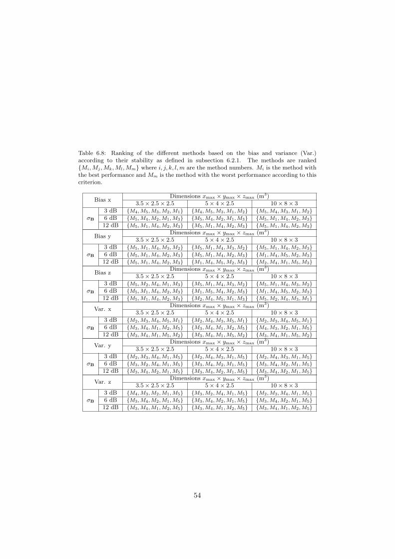
Table 6.8: Ranking of the different methods based on the bias and variance (Var.)according to their stability as defined in subsection 6.2.1. The methods are rankedMi,Mj ,Mk,Ml,Mm where i, j, k, l,m are the method numbers. Mi is the method withthe best performance and Mm is the method with the worst performance according to thiscriterion.

Bias xDimensions xmax × ymax × zmax (m3)

3.5× 2.5× 2.5 5× 4× 2.5 10× 8× 3

σB

3 dB M4,M5,M3,M2,M1 M4,M5,M3,M1,M2 M5,M4,M3,M1,M26 dB M5,M4,M2,M1,M3 M5,M4,M2,M1,M3 M5,M1,M4,M2,M312 dB M5,M1,M4,M2,M3 M5,M1,M4,M2,M3 M5,M1,M4,M2,M3

Bias yDimensions xmax × ymax × zmax (m3)

3.5× 2.5× 2.5 5× 4× 2.5 10× 8× 3

σB

3 dB M5,M1,M4,M3,M2 M5,M1,M4,M3,M2 M5,M1,M4,M2,M36 dB M5,M1,M4,M2,M3 M5,M1,M4,M2,M3 M1,M4,M5,M2,M312 dB M5,M1,M4,M2,M3 M1,M4,M5,M2,M3 M2,M4,M1,M5,M3

Bias zDimensions xmax × ymax × zmax (m3)

3.5× 2.5× 2.5 5× 4× 2.5 10× 8× 3

σB

3 dB M5,M2,M4,M1,M3 M5,M1,M4,M3,M2 M5,M1,M4,M3,M26 dB M5,M1,M4,M2,M3 M1,M5,M4,M2,M3 M1,M4,M5,M2,M312 dB M5,M1,M4,M2,M3 M2,M4,M5,M1,M3 M5,M2,M4,M3,M1

Var. xDimensions xmax × ymax × zmax (m3)

3.5× 2.5× 2.5 5× 4× 2.5 10× 8× 3

σB

3 dB M2,M3,M4,M5,M1 M2,M4,M3,M5,M1 M2,M3,M4,M5,M16 dB M3,M4,M1,M2,M5 M3,M4,M1,M2,M5 M4,M3,M2,M1,M512 dB M3,M4,M1,M5,M2 M3,M4,M1,M5,M2 M3,M4,M1,M5,M2

Var. yDimensions xmax × ymax × zmax (m3)

3.5× 2.5× 2.5 5× 4× 2.5 10× 8× 3

σB

3 dB M2,M3,M4,M1,M5 M2,M4,M3,M1,M5 M2,M4,M3,M1,M56 dB M3,M2,M4,M1,M5 M3,M4,M2,M1,M5 M3,M4,M2,M1,M512 dB M3,M4,M2,M1,M5 M3,M4,M2,M1,M5 M3,M4,M2,M1,M5

Var. zDimensions xmax × ymax × zmax (m3)

3.5× 2.5× 2.5 5× 4× 2.5 10× 8× 3

σB

3 dB M4,M3,M2,M1,M5 M3,M2,M4,M1,M5 M2,M3,M4,M1,M56 dB M3,M4,M2,M1,M5 M3,M4,M2,M1,M5 M3,M4,M2,M1,M512 dB M3,M4,M1,M2,M5 M3,M4,M1,M2,M5 M3,M4,M1,M2,M5

54

The environment used to generate the results presented in this subsectionhas been chosen because of its similarity with a real environment as well asthat it offers some characteristics that can be observed in different simula-tion environments altogether in a single virtual indoor space and that arepresented in this subsection. We will begin by presenting the general resultsin table 6.9. The results presented in this subsection are obtained using theNelder-Mead algorithm but simulations have also been conducted using theSequential Quadratic Programming (SQP) algorithm with similar results.With the implementation of the methods used, some characteristics arise. Ifwe take the general example of a 5× 4× 2.5 m3 room with 6 dB of shadowfading (rather obstructed), we can see the behaviour shown graphically infigure 6.4. The characteristics are described below:

• It is possible to combine the least squares and the log likelihood ap-proaches to obtain an approach that often provides less variance atthe expense of higher bias, as method 3 shows.

• It is possible to combine the least squares and the log likelihood ap-proaches to obtain an approach that often provides less bias at theexpense of higher variance, as method 5 shows.

• It is possible to combine the least squares and the log likelihood ap-proaches to obtain an approach that provides a balanced bias andoften less or approximately equal variance than the initial approaches,as method 4 shows.

• It is possible to find combinations of least square and log likelihoodthat collaborate to obtain more balanced results in indoor areas.

Besides the points stated above, an important feature is that the meth-ods on which the rest are based behave differently depending on whetherthe target node position is close to the anchor nodes or further, or whetherthe target node position is close to the limits of the indoor space. More-over, whereas one of the basic methods presents better bias, the alternativemethod presents better variance, which enables us to merge these character-istics into balanced methods. All these effects can be observed in figure 6.4.The results are obtained averaging 150 realizations of the random variablethat models the shadow fading for each of the position described in table 6.5.Thus, it possible to generate a three dimensional virtual map that shows theappropriate method for a desired property, bias or variance, in a desired sub-space of the indoor environment. An example of such a three dimensionalvirtual map is presented in figure 6.5 for the bias of x in a 3.5 × 2.5 × 2.5m3 room at 6 dB of shadow fading standard deviation.

55

Table 6.9: Values of the bias and the variance measured in the simulation environment ofthe different methods under study expressed in relative form (%) with reference to the max-imum dimension (length, width, height) of the indoor space. The values v1, v2, v3, v4, v5correspond, respectively to methods 1 to 5.

Bias xDimensions xmax × ymax × zmax (m3)

3.5× 2.5× 2.5 5× 4× 2.5 10× 8× 3

σB

3 dB 4.41, 3.83, 4.02, 3.67, 3.69 4.32, 3.49, 3.96, 3.50, 3.49 3.76, 3.13, 3.21, 2.92, 2.87

6 dB 5.54, 5.07, 6.33, 5.12, 4.71 5.02, 4.15, 5.78, 4.36, 3.99 3.79, 3.20, 4.18, 3.39, 3.10

12 dB 9.22, 10.2, 11.9, 9.68, 8.97 8.19, 8.89, 11.3, 8.53, 8.06 6.44, 6.76, 8.79, 6.54, 6.43

Bias yDimensions xmax × ymax × zmax (m3)

3.5× 2.5× 2.5 5× 4× 2.5 10× 8× 3

σB

3 dB 6.25, 7.12, 6.86, 6.62, 6.15 4.98, 5.54, 5.40, 5.24, 4.74 3.95, 4.12, 4.20, 4.02, 3.65

6 dB 11.3, 11.8, 12.3, 11.5, 11.0 8.80, 9.55, 10.0, 9.12, 8.58 6.89, 7.94, 8.39, 7.39, 6.91

12 dB 17.4, 17.9, 18.8, 17.7, 17.0 15.8, 16.7, 17.5, 16.3, 15.8 13.8, 14.3, 15.3, 14.0, 14.3

Bias zDimensions xmax × ymax × zmax (m3)

3.5× 2.5× 2.5 5× 4× 2.5 10× 8× 3

σB

3 dB 4.60, 4.73, 4.99, 4.59, 4.24 7.35, 7.77, 7.70, 7.56, 7.06 15.2, 15.7, 15.4, 15.4, 15.0

6 dB 7.74, 8.37, 8.86, 8.02, 7.48 12.7, 13.4, 13.5, 13.1, 12.7 20.0, 20.4, 20.6, 20.2, 20.0

12 dB 12.9, 13.3, 14.3, 13.1, 12.6 17.3, 17.2, 17.8, 17.2, 17.1 22.6, 22.6, 22.8, 22.6, 22.6

Var. xDimensions xmax × ymax × zmax (m3)

3.5× 2.5× 2.5 5× 4× 2.5 10× 8× 3

σB

3 dB 4.92, 3.52, 3.67, 3.77, 4.20 6.73, 4.86, 5.17, 5.19, 5.83 12.7, 8.55, 9.47, 9.36, 10.3

6 dB 10.5, 11.5, 9.14, 10.3, 11.2 13.9, 15.6, 12.5, 13.7, 15.0 24.4, 28.1, 23.1, 23.8, 24.9

12 dB 27.0, 29.1, 22.0, 26.4, 28.8 35.6, 40.5, 30.4, 35.1, 38.1 66.6, 78.8, 60.3, 65.8, 67.7

Var. yDimensions xmax × ymax × zmax (m3)

3.5× 2.5× 2.5 5× 4× 2.5 10× 8× 3

σB

3 dB 8.00, 6.73, 7.03, 7.14, 7.86 8.11, 7.21, 7.44, 7.44, 8.23 11.4, 10.8, 10.8, 10.8, 12.1

6 dB 18.8, 17.2, 15.8, 17.4, 19.9 20.9, 19.3, 17.9, 19.4, 23.1 35.2, 33.3, 30.3, 32.5, 41.0

12 dB 29.3, 29.2, 23.6, 28.2, 33.1 40.0, 38.1, 31.5, 36.8, 45.6 76.7, 68.8, 59.4, 66.8, 89.0

Var. zDimensions xmax × ymax × zmax (m3)

3.5× 2.5× 2.5 5× 4× 2.5 10× 8× 3

σB

3 dB 5.05, 4.59, 4.59, 4.60, 5.00 10.8, 9.96, 10.0, 10.1, 11.0 32.3, 28.5, 29.8, 29.8, 32.9

6 dB 13.5, 13.7, 12.0, 13.1, 14.4 23.3, 22.6, 21.2, 22.3, 24.7 43.8, 41.4, 39.8, 41.2, 46.1

12 dB 27.8, 27.8, 22.9, 26.6, 29.7 34.7, 35.0, 30.3, 33.4, 37.8 51.2, 52.5, 45.8, 49.2, 56.2

56

1 2 3 4 5

4

4.5

5

5.5

Method number

Relativeerror(%

)

(a) Error x

1 2 3 4 58.5

9

9.5

10

Method number

Relativeerror(%

)(b) Error y

1 2 3 4 512.6

12.8

13

13.2

13.4

Method number

Relativeerror(%

)

(c) Error z

1 2 3 4 512.5

13

13.5

14

14.5

15

15.5

Method number

Relativevar.

(%)

(d) Var. x

1 2 3 4 5

18

19

20

21

22

23

Method number

Relativevar.

(%)

(e) Var. y

1 2 3 4 5

21.5

22

22.5

23

23.5

24

24.5

Method numberRelativevar.

(%)

(f) Var. z

Figure 6.4: Relative error and variance of the coordinates (x, y, z) of the target nodeaveraged for all the node locations considered in the simulation in a 5× 4× 2.5 m3 roomat 6 dB of shadow fading standard deviation. The errors are expressed in absolute value,but in the process of calculation of the error both negative and positive biases have beenconsidered.

0 0.5 1 1.5 2 2.5 3 3.501

230

0.5

1

1.5

2

2.5

3

5

5

2

5

2

2

5

2

5

2

5

3

2

5

3

3

2

3

1

1

1

1

5

x

5

3

3

3

5

3

1

3

4

5

4

1

5

2

4

2

5

2

2

5

2

5

5

4

y

z

Figure 6.5: Three dimensional virtual map of a 3.5 × 2.5 × 2.5 m3 room at 6 dB ofshadow fading standard deviation showing the best method for each subspace of the indoorenvironment concerning the bias of x. The thicker points represent the anchor nodeswhereas the best method is written next to each indoor position.

57

Chapter 7

Conclusions

This section summarized the results obtained throughout the work. It alsoprovides areas of research that could be of interest in the future.

7.1 Conclusions of the Work

The results that this work yields show that it is possible to mathematicallycombine classical estimation approaches, specifically least squares and log-normal function maximization, in order to statistically improve the overallbias and variance of localization methods. Both the bias and the variancehave been improved for the implementations of the localization algorithmsdescribed in this work.

The experimental and simulation results show that the localization ap-proaches based on RSS in indoor spaces are very subject to shadow fadingeffects. This is a serious drawback when the shadow fading is comparable tothe differences among the various path losses for each anchor node, whichis the situation in small indoor spaces. The reason for this negative effectsis the high variance rather than the bias. Results show that it is feasibleto obtain acceptable relative values of bias with the adequate conditions.However, the variance in small indoor spaces will lead to inaccurate results,despite the acceptable bias. The orientation of the antenna is also of greatimportance and having omnidirectional patterns is essential for the perfor-mance.

This work shows that the traditional approaches of least squares and log-likelihood maximization can be tuned in order to focus on good performanceregarding a specific aspect, bias or variance, of a specific dimension. x,y, or z. The results can yield improvements in algorithms that use theseapproaches, which can benefit from this concept and improve their accuracy.

The implementation of all algorithms can be done in various ways usingdifferent numerical approaches. There is a variety of techniques that canbe applied in order to numerically and statistically design alternatively the

58

algorithms described throughout this thesis, which may have an effect ontheir accuracy.

7.2 Future Work

Concerning very small indoor spaces, RSS shows high sensitivity to shadowfading and hence AOA, TOA or techniques based on interference analysisoffer better accuracy in this context. However, these techniques generallyinvolve high costs and complexity in comparison with RSS techniques. Thestudy of algorithms to improve and cheapen the existing AOA/TOA orinterference based techniques in order to apply them to indoor localizationor even to combine them with RSS techniques is of interest.

Moreover, the research on harvesters show promise in the field of WSNs,since this would significantly reduce the nuisance of changing batteries in asmart home environment. Thus, the development of harvesters adapted tosmart home environments is a useful area of research. In this regard, greatprogress can be achieved in the fields of electronics and chemistry throughthe design of omnidirectional antennas and of efficient power supply sourcesor harvesters. The use of novel fast distributed techniques for estimationand detection seems an important area to explore [117].

59

Bibliography

[1] C. G. Montenegro, J. P. Aspas, and J. E. C. Herrero, Sensors Ev-erywhere (Wireless Networks Technologies and Solutions). FundacionVodafone Espana, 2010.

[2] A. Boukerche, H. Oliveira, E. Nakamura, and A. Loureiro, “Localiza-tion systems for wireless sensor networks,” Wireless Communications,IEEE, vol. 14, pp. 6 –12, december 2007.

[3] G. Mao, B. Fidan, and B. D. Anderson, “Wireless sensor networklocalization techniques,” Computer Networks, vol. 51, no. 10, pp. 2529– 2553, 2007.

[4] T. Stoyanova, F. Kerasiotis, K. Efstathiou, and G. Papadopoulos,“Modeling of the rss uncertainty for rss-based outdoor localization andtracking applications in wireless sensor networks,” in Sensor Technolo-gies and Applications (SENSORCOMM), 2010 Fourth InternationalConference on, pp. 45 –50, july 2010.

[5] A. Koubaa, M. Ben Jamaa, and A. AlHaqbani, “An empirical analysisof the impact of rss to distance mapping on localization in wsns,” inCommunications and Networking (ComNet), 2012 Third InternationalConference on, pp. 1 –7, 29 2012-april 1 2012.

[6] K. Ho and Y. Chan, “Solution and performance analysis of geolocationby tdoa,” Aerospace and Electronic Systems, IEEE Transactions on,vol. 29, pp. 1311 –1322, oct 1993.

[7] M. Baunach, R. Kolla, and C. Mvihlberger, “Beyond theory: Devel-opment of a real world localization application as low power wsn,” inLocal Computer Networks, 2007. LCN 2007. 32nd IEEE Conferenceon, pp. 872 –884, oct. 2007.

[8] G. Mao and B. Fidan, Localization Algorithms and Strategies for Wire-less Sensor Networks. Information Science Reference, 1 ed., May 2009.

[9] D. min Chen and Y. Zhang, “Research of wsn localization algorithmbased on entropy function,” in Education Technology and Computer

60

Science, 2009. ETCS ’09. First International Workshop on, vol. 1,pp. 229 –233, march 2009.

[10] W. Lei and W. XiaoPeng, “A new wsn localization algorithm based onregularization method,” in Instrumentation and Measurement Tech-nology Conference (I2MTC), 2011 IEEE, pp. 1 –4, may 2011.

[11] S. Wang, Z. Huang, Y. Hou, Y. Zhang, and R. Cheng, “A novel col-laborative sparse-anchored localization algorithm and error analysisfor wsn,” in Wireless Communications, Networking and Mobile Com-puting, 2008. WiCOM ’08. 4th International Conference on, pp. 1 –4,oct. 2008.

[12] W. J. Dixon, “Ratios involving extreme values,” The Annals of Math-ematical Statistics, vol. 22, pp. 68–78, Mar. 1951. Mathematical Re-views number (MathSciNet): MR39953; Zentralblatt MATH identi-fier: 0044.14604.

[13] W. J. Dixon, “Processing data for outliers,” International BiometricSociety, vol. 9, pp. 74–89, Mar. 1953.

[14] C. Zhang, X. Zhou, C. Gao, and C. Wang, “On improving the precisionof localization with gross error removal,” in Distributed ComputingSystems Workshops, 2008. ICDCS ’08. 28th International Conferenceon, pp. 144 –149, june 2008.

[15] F. Reichenbach and D. Timmermann, “Indoor localization with lowcomplexity in wireless sensor networks,” in Industrial Informatics,2006 IEEE International Conference on, pp. 1018 –1023, aug. 2006.

[16] L. Gogolak, S. Pletl, and D. Kukolj, “Indoor fingerprint localizationin wsn environment based on neural network,” in Intelligent Systemsand Informatics (SISY), 2011 IEEE 9th International Symposium on,pp. 293 –296, sept. 2011.

[17] V. Kaseva, T. Hamalainen, and M. Hannikainen, “Range-free algo-rithm for energy-efficient indoor localization in wireless sensor net-works,” in Design and Architectures for Signal and Image Processing(DASIP), 2011 Conference on, pp. 1 –8, nov. 2011.

[18] Q. Tang, C. Sun, H. Wen, and Y. Liang, “Cross-layer energy efficiencyanalysis and optimization in wsn,” in Networking, Sensing and Control(ICNSC), 2010 International Conference on, pp. 138 –142, april 2010.

[19] H.-P. Tan, P. Lee, W. Seah, and Z. A. Eu, “Impact of power con-trol in wireless sensor networks powered by ambient energy harvesting(wsn-heap) for railroad health monitoring,” in Advanced Information

61

Networking and Applications Workshops, 2009. WAINA ’09. Interna-tional Conference on, pp. 804 –809, may 2009.

[20] H. Karl, A. Willig, and A. Wolisz, Wireless Sensor Networks: FirstEuropean Workshop, Ewsn 2004, Berlin, Germany, January 19-21,2004, Proceedings. Springer, Mar. 2004.

[21] “IEEE - about IEEE.” http://www.ieee.org/about/index.html.

[22] “IEEE 802.15.4.” http://www.ieee802.org/15/pub/TG4.html.

[23] P. Park, P. Di Marco, P. Soldati, C. Fischione, and K. H. Johansson,“A generalized markov model for an effective analysis of slotted ieee802.15.4,” in Proc. of IEEE International Conference on Mobile Ad-hoc and Sensor Systems 2009 (IEEE MASS 09), Macau SAR, P.R.C.,October 2009.

[24] “ZigBee alliance.” http://www.zigbee.org/.

[25] “ITU.” http://www.itu.int/en/Pages/default.aspx.

[26] “ISO.” http://www.iso.org/iso/home.html.

[27] R. K. Shevgaonkar, Electromagnetic Waves. Tata McGraw-Hill Edu-cation, Oct. 2005.

[28] U.A.Bakshi, A.V. Bakshi, and K.A. Bakshi, Antenna And Wave Prop-agation. Technical Publications, Jan. 2008.

[29] J. C. Lin and K. S. Nikita, Wireless Mobile Communication andHealthcare: Second International ICST Conference; Revised SelectedPapers. Springer, 2011.

[30] A. Ando, T. Ito, H. Yoshioka, H. Tsuboi, and H. Nakamura, “Effectsof receiver antenna height and polarization on received signal levelsat road level from transmitter antennas set in manhole,” in Antennasand Propagation (APSURSI), 2011 IEEE International Symposiumon, pp. 2399 –2402, july 2011.

[31] C. Thongsopa, P. Sukphongchirakul, A. Intarapanich, andP. Jarataku, “Measurement of uhf signal strength propagating fromroad surface with vehicle obstruction,” 2010.

[32] “Echo 11 antenna family. siretta antennas.”http://www.siretta.co.uk/family.php?id=264.

[33] “Echo 1 antenna family siretta antennas.”http://www.siretta.co.uk/family.php?id=252.

62

[34] “gigaNOVA standard antennas.” http://www.antenova.com/gigaNOVA%20Standard%20Antennas.htm.

[35] “Fractus documentation for standard fractal antenna products.”http://www.fractus.com/index.php/fractus/documentation/#row2.

[36] “MEMSIC: wireless modules, IRIS, MicaZ, TelosB, imote2,cricket.” http://www.memsic.com/products/wireless-sensor-networks/wireless-modules.html.

[37] J. Polastre, R. Szewczyk, and D. Culler, “Telos: enabling ultra-lowpower wireless research,” in Information Processing in Sensor Net-works, 2005. IPSN 2005. Fourth International Symposium on, pp. 364– 369, april 2005.

[38] “Alien technology - products - RFID tags.”http://www.alientechnology.com/tags/index.php.

[39] “About for siretta antennas.”http://www.siretta.co.uk/about.php.

[40] “About antenova.” http://www.antenova.com/About.htm.

[41] “Fractus corporate - wireless antennas for every requirement.”http://www.fractus.com/index.php/fractus/corporate/.

[42] “ISO/IEC 18000-6:2010 - information technology – radio fre-quency identification for item management – part 6: Param-eters for air interface communications at 860 MHz to 960 MHz.”http://www.iso.org/iso/iso catalogue/catalogue tc/catalogue detail.htm?csnumber=46149.

[43] “About NXP :: NXP semiconductors.”http://www.nxp.com/about.html.

[44] H.-P. Tan, A. Valera, and W. Koh, “Transmission power control in 2-dwireless sensor networks powered by ambient energy harvesting,” inPersonal Indoor and Mobile Radio Communications (PIMRC), 2010IEEE 21st International Symposium on, pp. 1671 –1676, sept. 2010.

[45] “Powerharvester receivers | wireless power solutions | powercast corp..”http://www.powercastco.com/products/powerharvester-receivers/.

[46] A. F. Molisch, Wireless Communications. John Wiley & Sons, Dec.2010.

[47] J. S. Seybold, Introduction to RF Propagation. Wiley-Interscience,1 ed., Sept. 2005.

63

[48] “P.1238 : Propagation data and prediction methods for the planning ofindoor radiocommunication systems and radio local area networks inthe frequency range 900 MHz to 100 GHz.” http://www.itu.int/rec/R-REC-P.1238/en.

[49] T. S. Rappaport, Wireless Communications. Prentice Hall, 1st ed.,Jan. 1996.

[50] A. Goldsmith, Wireless Communications. Cambridge UniversityPress, Aug. 2005.

[51] E. Damosso, Digital Mobile Radio Towards Future Generation Sys-tems: COST Action 231. European Commission, 1999.

[52] A. Motley and J. Keenan, “Personal communication radio coveragein buildings at 900 mhz and 1700 mhz,” Electronics Letters, vol. 24,pp. 763 –764, jun 1988.

[53] M. Lott and I. Forkel, “A multi-wall-and-floor model for indoor radiopropagation,” in Vehicular Technology Conference, 2001. VTC 2001Spring. IEEE VTS 53rd, vol. 1, pp. 464 –468 vol.1, 2001.

[54] V. Erceg, L. Greenstein, S. Tjandra, S. Parkoff, A. Gupta, B. Kulic,A. Julius, and R. Jastrzab, “An empirically-based path loss model forwireless channels in suburban environments,” in Global Telecommuni-cations Conference, 1998. GLOBECOM 1998. The Bridge to GlobalIntegration. IEEE, vol. 2, pp. 922 –927 vol.2, 1998.

[55] S. Ghassemzadeh, L. Greenstein, A. Kavcic, T. Sveinsson, andV. Tarokh, “Uwb indoor path loss model for residential and com-mercial buildings,” in Vehicular Technology Conference, 2003. VTC2003-Fall. 2003 IEEE 58th, vol. 5, pp. 3115 – 3119 Vol.5, oct. 2003.

[56] D. Akerberg, “Properties of a tdma pico cellular office communica-tion system,” in Vehicular Technology Conference, 1989, IEEE 39th,pp. 186 –191 vol.1, may 1989.

[57] S. Seidel and T. Rappaport, “914 mhz path loss prediction models forindoor wireless communications in multifloored buildings,” Antennasand Propagation, IEEE Transactions on, vol. 40, pp. 207 –217, feb1992.

[58] D. Devasirvatham, C. Banerjee, M. Krain, and D. Rappaport, “Multi-frequency radiowave propagation measurements in the portable ra-dio environment,” in Communications, 1990. ICC ’90, IncludingSupercomm Technical Sessions. SUPERCOMM/ICC ’90. ConferenceRecord., IEEE International Conference on, pp. 1334 –1340 vol.4, apr1990.

64

[59] S. O. Rice, Mathematical analysis of random noise / by S.O. Rice.[New York] : American Telephone and Telegraph Co, 1944. Covertitle.

[60] M. Nakagami, “The m-distribution – A general formula of intensitydistribution of rapid fading,” in Statistical Methods in Radio WavePropagation (W. C. Hoffmann, ed.), 1960.

[61] A. M. Chen and R. Rao, “On tractable wireless channel models,” inPersonal, Indoor and Mobile Radio Communications, 1998. The NinthIEEE International Symposium on, vol. 2, pp. 825 –830 vol.2, sep 1998.

[62] A. Saleh and R. Valenzuela, “A statistical model for indoor multipathpropagation,” Selected Areas in Communications, IEEE Journal on,vol. 5, pp. 128 –137, february 1987.

[63] G. Turin, F. Clapp, T. Johnston, S. Fine, and D. Lavry, “A statisticalmodel of urban multipath propagation,” Vehicular Technology, IEEETransactions on, vol. 21, pp. 1 – 9, feb 1972.

[64] H. Suzuki, “A statistical model for urban radio propogation,” Com-munications, IEEE Transactions on, vol. 25, pp. 673 – 680, jul 1977.

[65] H. Hashemi, “The indoor radio propagation channel,” Proceedings ofthe IEEE, vol. 81, pp. 943 –968, jul 1993.

[66] “ETS 300 320.” http://webapp.etsi.org/workprogram/Report WorkItem.asp?WKI ID=27760&curItemNr=1&totalNrItems=14&optDisplay=10&qSORT=HIGHVERSION&qETSI ALL=&SearchPage=TRUE&qETSI NUMBER=300+328&qINCLUDE SUB TB=True&qINCLUDE MOVED ON=&qSTOP FLG=&qKEYWORD BOOLEAN=&qSTOPPING OUTDATED=&butSimple=Search&includeNonActiveTB=FALSE&includeSubProjectCode=&qREPORT TYPE=SUMMARY.

[67] “Home | FCC.gov.” http://www.fcc.gov/.

[68] R. de Souza and R. Lins, “A new propagation model for 2.4 ghz wire-less lan,” in Communications, 2008. APCC 2008. 14th Asia-PacificConference on, pp. 1 –5, oct. 2008.

[69] T. Chrysikos, G. Georgopoulos, and S. Kotsopoulos, “Wireless channelcharacterization for a home indoor propagation topology at 2.4 ghz,”in Wireless Telecommunications Symposium (WTS), 2011, pp. 1 –10,april 2011.

[70] G. Janssen, P. Stigter, and R. Prasad, “Wideband indoor channel mea-surements and ber analysis of frequency selective multipath channelsat 2.4, 4.75, and 11.5 ghz,” Communications, IEEE Transactions on,vol. 44, pp. 1272 –1288, oct 1996.

65

[71] T. Chrysikos, G. Georgopoulos, and S. Kotsopoulos, “Attenuation overdistance for indoor propagation topologies at 2.4 ghz,” in Computersand Communications (ISCC), 2011 IEEE Symposium on, pp. 329 –334, 28 2011-july 1 2011.

[72] I. Ahmed, S. Orfali, T. Khattab, and A. Mohamed, “Characteriza-tion of the indoor-outdoor radio propagation channel at 2.4 ghz,” inGCC Conference and Exhibition (GCC), 2011 IEEE, pp. 605 –608,feb. 2011.

[73] B. Sujak, D. Ghodgaonkar, B. Ali, and S. Khatun, “Indoor propaga-tion channel models for wlan 802.11b at 2.4 ghz ism band,” in AppliedElectromagnetics, 2005. APACE 2005. Asia-Pacific Conference on,p. 5 pp., dec. 2005.

[74] S. Reynaud, Y. Cocheril, R. Vauzelle, A. Reineix, L. Aveneau, andC. Guiffaut, “Influence of an accurate environment description for theindoor propagation channel modelling,” in Wireless Technology, 2005.The European Conference on, pp. 51 –54, oct. 2005.

[75] J. H. Yoo, J. H. Lee, and S. H. Cho, “A propagation model in 2.4ghzism band using ieee 802.15.4 systems,” in Communications (APCC),2011 17th Asia-Pacific Conference on, pp. 339 –343, oct. 2011.

[76] A. Ali, O. Aly, and A. Omar, “High resolution wlan indoor channelparameter estimation and measurements for communication and po-sitioning applications at 2.4, 5.2 and 5.8 ghz,” in Radio and WirelessSymposium, 2006 IEEE, pp. 279 – 282, jan. 2006.

[77] H. MacLeod, C. Loadman, and Z. Chen, “Experimental studies of the2.4-ghz ism wireless indoor channel,” in Communication Networks andServices Research Conference, 2005. Proceedings of the 3rd Annual,pp. 63 – 68, may 2005.

[78] H.-J. Zepernick and T. Wysocki, “Multipath channel parameters forthe indoor radio at 2.4 ghz ism band,” in Vehicular Technology Con-ference, 1999 IEEE 49th, vol. 1, pp. 190 –193 vol.1, jul 1999.

[79] T. Chrysikos, G. Georgopoulos, and S. Kotsopoulos, “Empirical calcu-lation of shadowing deviation for complex indoor propagation topolo-gies at 2.4 ghz,” in Ultra Modern Telecommunications Workshops,2009. ICUMT ’09. International Conference on, pp. 1 –6, oct. 2009.

[80] E. Walker, H.-J. Zepernick, and T. Wysocki, “Fading measurementsat 2.4 ghz for the indoor radio propagation channel,” in BroadbandCommunications, 1998. Accessing, Transmission, Networking. Pro-ceedings. 1998 International Zurich Seminar on, pp. 171 –176, feb1998.

66

[81] Y. Sun and L. Peng, “The simulation and analysis of uwb modified s-vchannel model,” in Wireless Communications, Networking and MobileComputing, 2009. WiCom ’09. 5th International Conference on, pp. 1–4, sept. 2009.

[82] S. Howard and K. Pahlavan, “Measurement and analysis of the in-door radio channel in the frequency domain,” Instrumentation andMeasurement, IEEE Transactions on, vol. 39, pp. 751 –755, oct 1990.

[83] K.-W. Cheung, J.-M. Sau, and R. Murch, “A new empirical model forindoor propagation prediction,” Vehicular Technology, IEEE Trans-actions on, vol. 47, pp. 996 –1001, aug 1998.

[84] D. Devasirvatham, “A comparison of time delay spread and signallevel measurements within two dissimilar office buildings,” Antennasand Propagation, IEEE Transactions on, vol. 35, pp. 319 – 324, mar1987.

[85] S. Cotton and W. Scanlon, “Characterization and modeling of the in-door radio channel at 868 mhz for a mobile bodyworn wireless personalarea network,” Antennas and Wireless Propagation Letters, IEEE,vol. 6, pp. 51 –55, 2007.

[86] S. Cotton, W. Cully, W. Scanlon, and J. McQuiston, “Channel char-acterisation for indoor wearable active rfid at 868 mhz,” in Antennasand Propagation Conference (LAPC), 2011 Loughborough, pp. 1 –4,nov. 2011.

[87] E. Tanghe, W. Joseph, L. Verloock, L. Martens, H. Capoen,K. Van Herwegen, and W. Vantomme, “The industrial indoor channel:large-scale and temporal fading at 900, 2400, and 5200 mhz,” WirelessCommunications, IEEE Transactions on, vol. 7, pp. 2740 –2751, july2008.

[88] M. Woehrle, M. Bor, and K. Langendoen, “868 mhz: a noiseless en-vironment, but no free lunch for protocol design,” in 9th int. conf. onNetworked Sensing Systems, INSS, pp. 1–8, jun 2012.

[89] Y. Xu, V. Gupta, and C. Fischione, “Distributed estimation,” in E-Reference Signal Processing, R. Chellappa and S. Theodoridis Eds.,Elzevir, to Appear, 2013.

[90] A. Speranzon, C. Fischione, K. H. Johansson, and A. Sangiovanni-Vincentelli, “A distributed minimum variance estimator for sensornetworks,” in IEEE Journal on Selected Areas in Communications,special issue on Control and Communications, vol. 26, N.4, pp. 609–621, May 2008.

67

[91] A. Speranzon, C. Fischione, and K. H. Johansson, “Distributed andcollaborative estimation over wireless sensor networks,” in Proc. ofIEEE 45th Conference on Decision and Control 2006 (IEEE CDC06), San Diego, USA, December 2006.

[92] S. M. Kay, Fundamentals of Statistical Signal Processing, Volume I:Estimation Theory. Prentice Hall, 1 ed., Apr. 1993.

[93] R. E. Kalman, “A New Approach to Linear Filtering and PredictionProblems,” Transactions of the ASME Journal of Basic Engineering,no. 82 (Series D), pp. 35–45, 1960.

[94] G. J. Pottie and W. J. Kaiser, Principles of Embedded Networked Sys-tems Design. Cambridge University Press, Oct. 2005.

[95] X. Zhao, L. Razouniov, and L. Greenstein, “Path loss estimation al-gorithms and results for rf sensor networks,” in Vehicular TechnologyConference, 2004. VTC2004-Fall. 2004 IEEE 60th, vol. 7, pp. 4593 –4596 Vol. 7, sept. 2004.

[96] A. Fanimokun and J. Frolik, “Effects of natural propagation environ-ments on wireless sensor network coverage area,” in System Theory,2003. Proceedings of the 35th Southeastern Symposium on, pp. 16 –20, march 2003.

[97] S. Tennina, M. Di Renzo, F. Graziosi, and F. Santucci, “Locating zig-bee R© nodes using the ti R©s cc2431 location engine: a testbed platformand new solutions for positioning estimation of wsns in dynamic indoorenvironments,” in Proceedings of the first ACM international workshopon Mobile entity localization and tracking in GPS-less environments,MELT ’08, (New York, NY, USA), pp. 37–42, ACM, 2008.

[98] G. Mao, B. D. Anderson, and B. Fidan, “Path loss exponent esti-mation for wireless sensor network localization,” Computer Networks,vol. 51, pp. 2467–2483, July 2007.

[99] G. Mao, B. Anderson, and B. Fidan, “Wsn06-4: Online calibrationof path loss exponent in wireless sensor networks,” in Global Telecom-munications Conference, 2006. GLOBECOM ’06. IEEE, pp. 1 –6, 272006-dec. 1 2006.

[100] G. M. Crippen and T. F. Havel, Distance Geometry and MolecularConformation. Research Studies Press, Oct. 1988.

[101] L. M. Blumenthal, Theory and Applications of Distance Geometry.Chelsea House Pub (L), 2nd ed., Nov. 1970.

68

[102] Y. Zhu, Multisensor Decision and Estimation Fusion. Springer, 1 ed.,Nov. 2002.

[103] S. Srinivasa and M. Haenggi, “Path loss exponent estimation in largewireless networks,” in Information Theory and Applications Work-shop, 2009, pp. 124 –129, feb. 2009.

[104] S. Srinivasa and M. Haenggi, “Modeling Interference in Finite Uni-formly Random Networks,” in International Workshop on InformationTheory for Sensor Networks (WITS 2007), (Santa Fe, NM), June 2007.Available at http://www.nd.edu/~mhaenggi/pubs/wits07.pdf.

[105] X. Li, “Rss-based location estimation with unknown pathloss model,”Wireless Communications, IEEE Transactions on, vol. 5, pp. 3626–3633, december 2006.

[106] R. Zemek, S. Hara, K. Yanagihara, and K.-i. Kitayama, “A joint es-timation of target location and channel model parameters in an ieee802.15.4-based wireless sensor network,” in Personal, Indoor and Mo-bile Radio Communications, 2007. PIMRC 2007. IEEE 18th Interna-tional Symposium on, pp. 1 –5, sept. 2007.

[107] J. Rodas and C. Escudero, “Joint estimation of position and channelpropagation model parameters in a bluetooth network,” in Communi-cations Workshops, 2009. ICC Workshops 2009. IEEE InternationalConference on, pp. 1 –5, june 2009.

[108] A. Doucet, S. Godsill, and C. Andrieu, “On sequential monte carlosampling methods for bayesian filtering,” STATISTICS AND COM-PUTING, vol. 10, no. 3, pp. 197–208, 2000.

[109] S. Maskell and N. Gordon, “A tutorial on particle filters for on-linenonlinear/non-gaussian bayesian tracking,” in Target Tracking: Algo-rithms and Applications (Ref. No. 2001/174), IEE, vol. Workshop,pp. 2/1 – 2/15 vol.2, oct. 2001.

[110] E. Hernandez-Perez, J. Navarro-Mesa, S. Martin-Gonzalez,P. Quintana-Morales, and A. Ravelo-Garcıa, “Path loss factorestimation for rss-based localization algorithms with wireless sensornetworks,” in 19th European Signal Processing Conference (EUSIPCO2011), Barcelona, Spain, 2011.

[111] G. H. Golub and C. F. v. V. Loan, Matrix Computations (Johns Hop-kins Studies in Mathematical Sciences. The Johns Hopkins UniversityPress, 3rd ed., Oct. 1996.

[112] S. Kay and Y. Eldar, “Rethinking biased estimation [lecture notes],”Signal Processing Magazine, IEEE, vol. 25, pp. 133 –136, may 2008.

69

[113] K. Yu and Y. Guo, “Efficient location estimators in nlos environ-ments,” in Personal, Indoor and Mobile Radio Communications, 2007.PIMRC 2007. IEEE 18th International Symposium on, pp. 1 –5, sept.2007.

[114] J. Andersen, T. Rappaport, and S. Yoshida, “Propagation measure-ments and models for wireless communications channels,” Communi-cations Magazine, IEEE, vol. 33, pp. 42 –49, jan 1995.

[115] S. Lohier, A. Rachedi, E. Livolant, and I. Salhi, “Wireless sen-sor network simulators relevance compared to a real ieee 802.15.4testbed,” in Wireless Communications and Mobile Computing Con-ference (IWCMC), 2011 7th International, pp. 1347 –1352, july 2011.

[116] R. Peng and M. Sichitiu, “Robust, probabilistic, constraint-based lo-calization for wireless sensor networks,” in Sensor and Ad Hoc Com-munications and Networks, 2005. IEEE SECON 2005. 2005 SecondAnnual IEEE Communications Society Conference on, pp. 541 – 550,sept., 2005.

[117] C. Fischione, “Fast-Lipschitz optimization with wireless sensor net-works applications,” in IEEE Transactions on Automatic Control,vol. 56, No.10, pp. 2319–2331, October 2011.

70