Indo - Norway Project Sustainable Transport Measures for ...
163
Indo - Norway Project Sustainable Transport Measures for Liveable Bengaluru Prof. Ashish Verma Mr. Harsha Vajjarapu Ms. Hemanthini Allirani Transportation Engineering Lab, Department of Civil Engineering, Indian Institute of Science (IISc), Bangalore APRIL, 2018
Transcript of Indo - Norway Project Sustainable Transport Measures for ...

Indo - Norway Project
Sustainable Transport Measures for
Liveable Bengaluru
Prof. Ashish VermaMr. Harsha Vajjarapu
Ms. Hemanthini AlliraniTransportation Engineering Lab,Department of Civil Engineering,
Indian Institute of Science (IISc), Bangalore
APRIL, 2018

Project Expert Team
Principal Investigator
Prof. Ashish Verma
Associate Professor, Department of Civil Engineering
Indian Institute of Science, Bangalore
Email ID: [email protected]
Other Project Partners
1. Dr. Farideh Ramjerdi Institute of Transport Economics (TØI)
Project Manager & Principal Investigator
2. Dr. Sanjay Gupta
School of Planning & Architecture, New Delhi
Principal Investigator
3. Dr. Munish Chandel
Indian Institute of Technology, Bombay
Principal Investigator
4. Dr. Hilde Fagerli
Norwegian Meteorological Institute (MET)
Principal Investigator
5. Ms. Neha Pahuja
The Energy & Resource Institute (TERI), New Delhi
Principal Investigator
Research Staff
1. Mr. Harsha Vajjarapu (Research Scholar) 2. Ms. Hemanthini Allirani (Junior Research Fellow)
Project Funded by
Research Council of Norway (https://www.toi.no/climatrans/category1492.html)
Preferred Citation
Verma A., Harsha V., Hemanthini AR. (2018), “Sustainable Transport Measures for
Liveable Bengaluru”, Project Sub Report, IISc Bangalore, India.
Note: This is a sub report. The full report containing all the case cities Bengaluru, New Delhi and Mumbai will
be released soon.

Sustainable Transport Measures for Liveable Bengaluru
Transportation Engineering Lab, Department of Civil Engineering, IISc Bangalore Page ii
ACKNOWLEDGEMENT
The successful completion of this research work was possible only due to the immense
support and relentless cooperation by the following people and organizations.
We are grateful to Research Council of Norway for providing us with the necessary
funding to carry out this project. Special thanks to Dr. Farideh Ramjerdi, Dr. Sanjay Gupta,
Dr. Munish Chandel, Dr. Hilde fagerli and Ms. Neha Pahuja for their valuable inputs and
support throughout the project.
Our sincere thanks to all the stakeholders from the following organizations of Bangalore
Metropolitan Region for their active participation in the stakeholder meetings and their
valuable inputs, as well as data which served as the basis for this study.
Bangalore Development Authority
Bangalore Metropolitan Region Development Authority
Bangalore Metropolitan Transport Corporation
Directorate of Urban Land Transport
Bangalore Metro Rail Corporation Ltd.
Karnataka Pollution Control Board
Karnataka Slum Development Board
Bruhat Bengaluru Mahanagara Palike
Directorate of Economics & Statistics, Karnataka
Directorate of Census Operations
We would also like to acknowledge the contribution of Mrs. Mehvish Shah,
Mrs. Girija Umashankar, Mr. Saqib Gulzar, Ms. Swarnali Dihingia, Ms. Nikhita Rodeja and
Ms. Sajitha Sasidharan the ex-research fellows at Indian Institute of Science Bangalore
whose work served as a base reference for this study.
Last but not the least; we would like to thank Indian Institute of Science Bangalore for
providing institutional support necessary for the smooth running of the project. Our
gratitude goes to the Chairman, Civil Engineering Department for extending the facilities
of the department for various meetings.
- Project Team

Sustainable Transport Measures for Liveable Bengaluru
Transportation Engineering Lab, Department of Civil Engineering, IISc Bangalore Page iii
ABSTRACT
India is one of the fastest urbanizing countries in the world and the urban centres share
a major part in improving nation’s economy. Growing economies have led to employment
opportunities which in turn lead to a lot of migration to the cities. Rapidly growing
economies coupled with urbanization pose a great threat to the resilience, sustainability
and liveability of the cities. Increasing urban population and motorization in most of the
Asian countries are bound to raise road congestion and environmental pollution making
cities difficult to live. Recently, liveability has received more importance due to the
degrading condition in the quality of life in metropolitan cities. Mobility is a major
concern in many Indian cities, due to inadequate transport infrastructure, increased
usage of private vehicles, traffic congestion, pollution and lack of integration between
land use and transport planning thus, undermining the cities’ efforts to meet global
standards of living. Recently, the Government of India has also formulated 79 indicators
in 15 categories in order to measure the liveability standards of 116 Indian cities focusing
on four main aspects such as institutional, social, economic and physical that affects the
quality of life.
This report is an outcome of last 4 years of research work under an Indo-Norway project
CLIMATRANS to develop and evaluate sustainable transport measures that improves the
liveability of Indian cities including, Bengaluru, Delhi, and Mumbai. The current report
presents only the case study of Bengaluru Metropolitan Region (BMR) which includes
Bengaluru urban district, Bengaluru rural district and Ramnagara covering an area of
about 8005 sq.km. BMR is one of the rapidly urbanizing metropolitan area with 584%
increase in the city’s built up area in the past four decades. The increased population in
urban areas eventually led to increased vehicle usage in the limited city’s infrastructure
causing traffic congestion, longer travel times and pollution, making it hard to live in the
city. Also, due to concretization of land, encroachment of water bodies, improper
maintenance of drainage facilities has resulted in higher runoff on the roads getting the
city transportation sector to a halt and thereby reducing the resiliency of the
transportation system in the city. This report details about the quantitative evaluation of
sustainable transport mitigation and adaptation measures aimed to improve the
liveability of Bengaluru in terms of; reduced traffic congestion (VKT), reduced exhaust
emissions (PM, CO, NOX, HC etc.), reduced greenhouse gas emissions (CO2), reduced
carbon emission intensity w.r.t. GDP growth, increased consumer surplus of sustainable
modes, and also improved resiliency of transportation system. The same was done by
comparing the Business as Usual scenario and various sustainable transport scenarios,
for the base year and the future years 2030 and 2050. It is expected that the findings of
this report will provide more scientific and evidence based decision support for framing
right kind of sustainable transport planning and policy measures to make Bengaluru
more liveable. Also, the basic principles and developed methodology from this study can
be applied to other Indian cities as well to develop similar measures aimed at improving
their liveability.

Sustainable Transport Measures for Liveable Bengaluru
Transportation Engineering Lab, Department of Civil Engineering, IISc Bangalore Page iv
EXECUTIVE SUMMARY
Rapidly growing economies and subsequent increase in private vehicle usage pose a
threat to the sustainable development of most of the developing cities worldwide.
Increasing urban population and motorization in most of the Asian countries are bound
to raise road congestion and environmental pollution. Sustainable transport measures
are seen as a tool to reduce the vulnerability to the potential negative impacts of
urbanization. Transportation being a critical sector contributes to the smooth functioning
of societies and fosters economic growth of a nation. Bengaluru is a good example of rapid
urbanization, which is evident from the fact that the city added about two million people
in just the last decade. In the history of Bengaluru, the highest growth in population of
106% is recorded in the last two decades. Although Bengaluru’s rapid economic growth
has substantially improved the local quality of life, yet challenging issues of urbanization,
motorization, congestion & pollution looms over the development of the city. Bengaluru’s
infrastructure and urban planning has not kept pace with its rapidly increasing
population and the growing number of vehicles on the road. This study has been carried
out to address the issue by quantitative evaluation of sustainable transport mitigation
and adaptation measures aimed to improve the liveability of Bengaluru in terms of;
reduced traffic congestion (VKT), reduced exhaust emissions (PM, CO, NOX, HC etc.),
reduced greenhouse gas emissions (CO2), reduced carbon emission intensity with respect
to GDP growth, increased consumer surplus of sustainable modes, and also improved
resiliency of transportation system. The main objectives of the study are:
1) Developing mitigation strategies for transportation sector which are aimed at
reducing the GHG emissions, local pollutants and traffic congestion from a baseline
condition. These mitigation strategies will be developed for two scenarios which
are Business as usual scenario and sustainable transport Scenario for the base
year and the future years 2030 and 2050.
2) Identification of the transportation infrastructure that is vulnerable to climate
change and assess the impacts of climate change on the transportation
infrastructure.
3) Developing adaptation strategies for the base year and the horizon years 2030 &
2050 to evaluate the vulnerability, scope & extent, severity of each flood event
caused by climate change to transportation sector.
4) Improving the overall liveability of Bengaluru.
The demographics & mobility of the BMR region for the base year 2008 is studied and
forecasted for the years 2030 & 2050 as a part of Business as Usual scenario (BAU). The
mitigation and adaptation strategies are developed to estimate and evaluate the effects
of each policy on the BAU scenario for the years 2030 & 2050. Bengaluru is the most
urbanized district with 90.94% of its population residing in urban areas. Traffic problems
are diverse and complex ranging from low speeds, long travel times and the peak hour
travel speed in the city is less than 17 km/hr (CTTS report, 2010). Personalized modes of

Sustainable Transport Measures for Liveable Bengaluru
Transportation Engineering Lab, Department of Civil Engineering, IISc Bangalore Page v
transport have grown at a tremendous rate and two wheelers along with the cars almost
comprise 90% of the total registered vehicular population in the city. The population
living in urban slums in Karnataka has risen from 1.402 million (2001) to 3.291 million
(2011) in a decade.
Business as Usual scenario - Mitigation
Mitigation: Mitigation is defined as “an anthropogenic intervention to reduce the sources
or enhance the sinks of greenhouse gases” (IPCC, 2001a). Mitigation can mean using new
technologies and renewable energies, making older equipment more energy efficient,
changing management practices or consumer behaviour.
The total population of the BMR region as per the census in 2001 is 8.5 million and in
2011 is 10.8 million. The source for this data was taken from Comprehensive Traffic and
Transportation Studies (CTTS) report and has been projected to 2030 and 2050. It is
estimated that the population would reach 18 million by 2030 and 33 million by 2050.
The study estimated that the average trip length for the base year for BMR is 14 km and
11 km for private and public transport respectively and has increased for the years 2030
and 2050 as shown in the table below.
Table I: Comparison of average trip lengths
With majority of the population opting for public transport as their mode of travel, it has
a mode share of 49.7 % with the least being car (2.3%). Mode share of two wheelers is
28.9%, 3 wheelers (Auto) 3.7% and NMT share is about 15.4%. The future projections of
mode share for the years 2030 and 2050 are shown in Figure below.
Figure I: Estimated mode share for the years 2030 and 2050
The ratio of Bangalore Metropolitan Transport Corporation (BMTC) to BMRCL mode
share is taken out from the report and applied to the model to estimate the modal share
Average Trip Length (km)
Year Private Transport Public Transport
Base Year 14.1 11.4
2030 17.41 16.36
2050 18.17 18.22
5.1
17.4
35.73
17.87
4.6
19.3
Estimated Modal Split for 2050
Car 2w Bus Metro Auto NMT
3.9
23.5
34.53
17.27
4
16.8
Estimated Modal Split for 2030
Car 2w Bus Metro Auto NMT

Sustainable Transport Measures for Liveable Bengaluru
Transportation Engineering Lab, Department of Civil Engineering, IISc Bangalore Page vi
of BMRCL for 2030 and 2050. The total Vehicle Kilometres Travelled (VKT) by the
vehicles in the BMR region is about 31 million for the base year and is estimated to
increase about 48 million and 72 million for the years 2030 and 2050 respectively which
is about 60% growth rate of VKT in 2050 from base year.
The vehicular emissions are dependent on Vehicle Kilometres Travelled. For this study 5
pollutants namely CO, HC, NOx, CO2, PM are considered. Emissions estimated for the
modes considered for the study are stated in the table below.
Table II: Total Emissions in Base Year, 2030 and 2050 (BAU Scenario)
Pollutant Emissions in Tonnes/ year (% change w.r.t Base Year)
Base Year 2030 2050
CO 15743 18179 (15%) 23567 (50%)
HC 7315 2930 (-60%) 3841 (-47%)
NOx 6985 28864 (313%) 22962 (229%)
CO2 695617 16782759 (2313%) 17662478 (2439%)
PM 973 2009 (106%) 1519 (56%)
Mitigation Policy Scenarios
Based on the IPCC definition, inputs from multiple stakeholder meetings and Delphi
survey with various government officials of Bengaluru, 4 policy bundles are formulated.
The main objective of these mitigation policy bundles is to attain an optimum balance of
push and pull strategy by developing policies that encourage public transportation and
also other sustainable modes. This helps in reducing the vehicle kilometres travelled
which leads to reduction in emissions and traffic congestion as compared to Business as
usual scenario thereby improving the quality of life of people in Bengaluru city.
Table III: Policy bundles for mitigation
Policies under bundle 1 Increasing network coverage of Public Transit Cycling and walking infrastructure Additional tax on purchasing vehicles Policies under bundle 2 Additional tax on purchasing vehicles Strict Vehicles inspection/Improvement in standards for vehicle emission Increase in fuel cost Policies under bundle 3 Increasing network coverage of Public Transit Defining car restricted roads Congestion Pricing Park and Ride Cycling and Walking infrastructure Encouraging car-pooling and High Occupancy Lanes High density mix building use along main transport corridors Policies under bundle 4 All policies in bundle 3 + All buses and cars running on electricity
Each bundle mentioned above is a mixture of various policy instruments. Bundle 1 is a
mixture of Planning & Regulatory Instruments. Bundle 2 is a mixture of Economic &

Sustainable Transport Measures for Liveable Bengaluru
Transportation Engineering Lab, Department of Civil Engineering, IISc Bangalore Page vii
Regulatory Instruments, bundle 3 is a mixture of Planning, Regulatory & Economic
Instruments and bundle 4 is a blend of planning, regulatory, economic and technology
instruments. The bundle 4 includes the assumption of electrification of all cars and buses
for horizon years. In addition, four different scenarios are assumed based on the different
projections of the energy mix in the target years as follows:
i. Scenario 1: New Policies Scenario (IEA, 2015) - Non-renewable sources &
Electricity (74% - 26%)
ii. Scenario 2: Electricity from non-renewable Sources (100 %)
iii. Scenario 3: Half electricity from renewable and another half from non-renewable
sources (50 % - 50 %)
iv. Scenario 4: Electricity from Renewable Sources (100 %)
Bundles are carefully evaluated and tested at various locations in BMR. It is observed that
Bundle 3 (also Bundle 4) which is a comprehensive mixture of 7 policies gives the best
results with respect to VKT reduction, Improved Public Transport Share and reduction in
emissions. The substantial reduction in emissions is observed with the implementation
of bundle 4 - scenario 4 where the electricity is assumed to be generated only from
renewable sources. The comparison of BAU 2030 with the 3 policy bundles is shown the
figures below.
Figure II: Mode share comparison between BAU and Policy Bundles for the year 2030
2.7
36
.4
17
.9
19
.4
3.7
15
.1
4.8
2.4
36
.5
18 18
.2
3.4
15
.9
5.6
2.1
37
.9
18
.6
16
.4
2.9
16
.2
5.9
3.9
34
.7
17
.1
23
.5
4
12
.7
4.1
C A R B U S M E T R O 2 W A U T O C Y C L E W A L K
M O D E S H A R E - 2 0 3 0
Bundle 1 Bundle 2 Bundle 3 & 4 BAU

Sustainable Transport Measures for Liveable Bengaluru
Transportation Engineering Lab, Department of Civil Engineering, IISc Bangalore Page viii
Figure III: Mode share comparison between BAU and Policy Bundles for the year 2050
Figure IV: VKT comparison for BAU and Policy Bundles for 2030 & 2050
It is clearly seen from the figures that the private transport mode share will reduce and
public transport and NMT mode share will increase across all the policy bundles, with
bundle 3 (also bundle 4) producing the best results. Due to increase in mode share of
public transport with high occupancy levels, the total vehicle kilometers travelled
reduces substantially when compared with BAU for 2030. Since emissions are a function
of vehicle kilometers travelled, it is seen that the emissions reduce across all bundles with
the bundle 4 - scenario 4 giving best results. In bundle 4 - scenario 4 it is observed that
the CO2 emissions were found to reduce by almost 98% for 2030 and 2050 when
compared with 2030 and 2050 BAU scenarios respectively. The emissions
comparison for the pollutant CO2 for bundles 1-4 with BAU scenario of 2030 and 2050 is
shown in Figures below.
2.5
33
.8
22
.5
14
.1
3.9
18
.1
5.1
2.2
34
.1
22
.7
13
.3
3.2
18
.3
6.2
1.8
35
23
.4
11
.1
2.8
19
.2
6.7
5.1
32
.2
21
.4
17
.4
4.6
14
.8
4.5
C A R B U S M E T R O 2 W A U T O C Y C L E W A L K
M O D E S H A R E - 2 0 5 0
Bundle 1 Bundle 2 Bundle 3 & 4 BAU
45
.7
45
.5
44
.8
47
70
.4
70
.1
69
.7
72
.1
B U N D L E 1 B U N D L E 2 B U N D L E 3 & 4 B A U
C O M P A R I S O N O F V K T ' S
Total VKT 2030(in millions) Total VKT 2050(in millions)
4.7 %
3.2 %

Sustainable Transport Measures for Liveable Bengaluru
Transportation Engineering Lab, Department of Civil Engineering, IISc Bangalore Page ix
*98% reduction in total CO2 emissions is observed in B4-S4 w.r.t. BAU. Further considering extreme scenario where electricity is
assumed to be purely generated from hydropower, solar and wind without using bio energy, 89% reduction in emission is observed
even in BAU scenario itself. Additionally, with the same assumption in B4-S4 scenario, 98% reduction in total CO2 emissions can be
achieved with respect to BAU scenario
Figure V: Total CO2 emissions in tonnes/year for 2030
*56% reduction in total percapita CO2 emissions is observed in B4-S4 w.r.t. BAU. Further considering extreme scenario where
electricity is assumed to be purely generated from hydropower, solar and wind without using bio energy, 3% reduction in emission is observed even in BAU scenario itself. Additionally, with the same assumption in B4-S4 scenario, 56% reduction in total percapita CO2 emissions can be achieved with respect to BAU scenario
Figure VI: Total Percapita CO2Emissions in kilo tonnes/person/Year for 2030
16
70
97
21
21
49
09
12
11
64
87
04
18
06
49
6
17
11
09
48
19
75
80
40
11
91
03
17
17
96
60
0
18
46
53
58
23
80
71
04
12
81
09
81
18
14
85
9
18
92
79
30
24
91
17
99
12
59
38
51
27
58
98
16
78
27
59
B1 - S1 B1 - S2 B1 - S3 B1 - S4 B2 - S1 B2 - S2 B2 - S3 B2 - S4B3 - S1 B3 - S2 B3 - S3 B3 - S4 B4 - S1 B4 - S2 B4 - S3 B4 - S4 BAU
TOTAL CO2 EMISSIONS IN TONNES/YEAR - 2030
98 %
*
22
5.3
63
0
22
7.1
48
5
22
3.4
73
1
21
9.7
97
7
22
3.3
96
8
22
4.3
79
8
22
1.4
65
5
21
7.7
09
7
22
6.4
61
1
22
8.3
80
8
22
4.4
29
0
22
0.4
77
2
19
3.1
01
4
22
3.0
33
4
16
1.4
12
6
99
.78
36
22
8.8
91
8B1 - S1 B1 - S2 B1 - S3 B1 - S4 B2 - S1 B2 - S2 B2 - S3 B2 - S4B3 - S1 B3 - S2 B3 - S3 B3 - S4 B4 - S1 B4 - S2 B4 - S3 B4 - S4 BAU
TOTAL PERCAPITA CO2 EMISSIONS IN KILO TONNES/PERSON/YEAR - 2030
56 %
*

Sustainable Transport Measures for Liveable Bengaluru
Transportation Engineering Lab, Department of Civil Engineering, IISc Bangalore Page x
* 98% reduction in total CO2 emissions is observed in B4-S4 w.r.t. BAU. Further considering extreme scenario where electricity is
assumed to be purely generated from hydropower, solar and wind without using bio energy, 82% reduction in emission is observed even in BAU scenario itself. Additionally, with the same assumption in B4-S4 scenario, 98% reduction in total CO2 emissions can be achieved with respect to BAU scenario
Figure VII: Total CO2 emissions in tonnes/year for 2050
* 56% reduction in total percapita CO2 emissions is observed in B4-S4 w.r.t. BAU. Further considering extreme scenario where
electricity is assumed to be purely generated from hydropower, solar and wind without using bio energy in B4-S4 scenario, 56% reduction in total percapita CO2 emissions can be achieved with respect to BAU scenario
Figure VIII: Total PercapitaCO2 Emissions in kilo tonnes/year for 2050
It can be seen that in Bundle 3 - Scenario 4 total CO2 emissions are higher compared to
Bundle 1 and bundle 2. This is because of high mode shift towards public transport. Since
buses have high emissions factors the total CO2 seems to be on the higher side. But from
the figure VIII it is clearly observed that the bundle 3 - Scenario 4 gives less per-capita
emissions compared to bundle 1 and bundle 2 since bus transport is shared by more
number of people. However, in bundle 4 - scenario 4 with electrification of buses and
generating electricity only from renewable sources demonstrates substantial reduction
in emissions. As per the Intended Nationally Determined Contributions (INDC), India
targets to reduce the emissions intensity of its GDP by 33% to 35% by 2030 from 2005
17
44
34
22
22
57
05
25
12
80
62
58
30
41
97
9
17
57
37
53
22
76
41
54
12
87
93
40
29
94
51
5
17
74
67
79
23
00
04
77
12
99
51
17
29
89
74
5
18
89
31
61
25
50
85
31
12
90
99
43
31
13
04
17
66
24
78
23
15
46
89
B1 -S1
B1 -S2
B1 -S3
B1 -S4
B2 -S1
B2 -S2
B2 -S3
B2 -S4
B3 -S1
B3 -S2
B3 -S3
B3 -S4
B4 -S1
B4 -S2
B4 -S3
B4 -S4
BAU RA
TOTAL CO2 EMISSIONS IN TONNES/YEAR - 2050
98 %
*
18
1.8
68
2
18
2.6
98
3
18
1.1
17
3
17
9.5
36
4
18
2.4
93
5
18
3.3
26
5
18
1.7
40
1
18
0.1
53
7
18
6.7
46
0
18
7.5
63
9
18
6.0
06
2
18
4.4
48
5
14
7.1
87
0
17
1.6
92
7
12
5.0
16
3
78
.34
69
17
7.7
76
7B1 - S1 B1 - S2 B1 - S3 B1 - S4 B2 - S1 B2 - S2 B2 - S3 B2 - S4B3 - S1 B3 - S2 B3 - S3 B3 - S4 B4 - S1 B4 - S2 B4 - S3 B4 - S4 BAU
TOTAL PERCAPITA CO2 EMISSIONS IN KILO TONNES/PERSON/YEAR - 2050
56 %
*

Sustainable Transport Measures for Liveable Bengaluru
Transportation Engineering Lab, Department of Civil Engineering, IISc Bangalore Page xi
Level. Since, the share of transportation is not mentioned the same intended percentage
has been assumed for transport sector.
Figure IX: Emissions Intensity comparison between BAU and Policy Bundles for 2030 and 2050
* The carbon emissions intensity is increasing at the greater rate in BAU 2030 and 2050 scenario because Metro is not available in
Bengaluru during base year and it is the only electricity based transportation with high emission factor values. Further considering
extreme scenario where electricity is assumed to be purely generated from hydropower, solar and wind without using bio energy in
BAU scenario, 39% reduction in total CO2 emission intensity can be achieved in BAU 2030 with respect to base year and 60%
reduction in total CO2 emission intensity can be achieved in BAU 2050 with respect to base year.
Figure X: Percentage reduction in Emission Intensity of BAU 2030, 2050 and Bundles from Base
year (2008)
The carbon emissions intensity is increasing at the greater rate in BAU 2030 scenario
because Metro is not available in Bengaluru during base year and it is the only electricity
based transportation with high emission factor values. The share of generation of
electricity from renewable and non-renewable sources plays a significant role in
emission intensity. The study clearly states that the emission reduction reaches the INDC
targets even for the BAU scenarios of 2030 and 2050 with the extreme scenario case of
assuming that the electricity will be purely generated from renewable sources. If the
bundle 4-scenario 4 is implemented the percapita emission intensity will reduce by 97%
for the year 2030 and 99% for 2050, highlighting that electrification of vehicles is the best
solution. Also, consumer surplus costs associated with bundles 1, 2 & 3 have been
40
.53 5
2.1
3
28
.26
4.3
8
41
.51
47
.93
28
.89
4.3
6
44
.79
57
.75
31
.08
4.4
0
45
.91
60
.43
30
.55
0.6
7
40
.71
16
.01
20
.71
11
.75
2.7
9
16
.13
20
.89
11
.82
2.7
5
16
.29
21
.11
11
.93
2.7
4
17
.34
23
.41
11
.85
0.2
9
16
.21
B1 - S1 B1 - S2 B1 - S3 B1 - S4 B2 - S1 B2 - S2 B2 - S3 B2 - S4 B3 - S1 B3 - S2 B3 - S3 B3 - S4 B4 - S1 B4 - S2 B4 - S3 B4 - S4 BAU
EMISSION INTENSITY (TONNES OF CO2/RS. CRORE)
2030 2050
44
4%
60
0%
27
9%
41
%
45
7% 54
3%
28
8%
41
%
50
1%
67
5%
31
7%
41
%
51
6%
71
1%
31
0%
91
%
44
7%
11
5%
17
8%
58
%
63
%
11
7%
18
0%
59
%
63
%
11
9%
18
3%
60
%
63
%
13
3%
21
4%
59
%
96
%
11
8%
B1 - S1 B1 - S2 B1 - S3 B1 - S4 B2 - S1 B2 - S2 B2 - S3 B2 - S4 B3 - S1 B3 - S2 B3 - S3 B3 - S4 B4 - S1 B4 - S2 B4 - S3 B4 - S4 BAU
REDUCTION IN EMISSION INTENSITY FROM BASE YEAR
2030 2050
*

Sustainable Transport Measures for Liveable Bengaluru
Transportation Engineering Lab, Department of Civil Engineering, IISc Bangalore Page xii
estimated and it was found that from bundle 3 consumers who use Public transportation
gain about Rs. 0.71 million for the year 2030 and Rs. 1.1 million for 2050 while the 2
wheeler users are at the major loss with Rs. 360 million for 2030 and Rs. 1220 million for
2050.
BAU Scenario for Adaptation
Bangalore Metropolitan Region flood map is prepared based on the heavy rainfall
occurred on November 3rd 2015 (total rainfall - 266mm, duration - 4 hrs 10 mins, return
period - 100 yrs) and it is overlaid over the BMR road network to extract the flood levels.
For the BAU network each road link is divided into multiple small links depending on the
level of flood in that particular link. The percentage share of flood depth on road network
of BMR is shown in the below figure. Links which carry a flood depth above 0.5 m are
considered to be not motorable in the BAU model. Roads that are heavily flooded and the
zones that do not have redundant roads for the trip to happen are considered to have no
trips from those zones. BAU modelling is done for the base year i.e., 2008 and for the
future years 2030, 2050 for both private and public transport networks. Since this is not
a frequent event and not a usual scenario the mode shift is kept the same even though
trip lengths change.
Figure XI: Percentage share of flood depth on BMR road network for the base year
Due to the flooding of roads, people who commute in their usual shortest paths change
their course which leads to longer paths and longer travel time.
28
35
9
14
64 3 2
Percentage Share of flood depth on road network (%)
0-0.01
0.01-0.1
0.1-0.2
0.2-0.3
0.3-0.4
0.4-0.5
0.5-2
2.0-9.0
Depth (m)

Sustainable Transport Measures for Liveable Bengaluru
Transportation Engineering Lab, Department of Civil Engineering, IISc Bangalore Page xiii
Figure XII: Comparison of VKT for flooding and No flooding scenarios for base year, 2030& 2050
Figure XIII: Comparison of VHT for flooding and No flooding scenarios for base year,
2030& 2050
It is observed that the average private transport trip lengths increase from 14.1 km in
BAU base year (no flood scenario) to 21.7 km in 2050 for a flood scenario. For public
transport the average trip lengths increase from 11.4 km in BAU base year no flooding
scenario to 20.4 km in 2050 flooding scenario. Also, the average daily vehicle speed
reduces from 27kmph in base year no flooding to 13kmph during flooding in 2050.
Adaptation Policy Scenarios
As discussed in the first section adaptive measures are seen as a tool to reduce the
vulnerability to the potential negative impacts of climate change and strengthen the
inherent capacity of a system to undertake defensive as well as protective actions that
help to avoid loss and facilitate recovery from any impact by increasing the resilience of
the entire system.
The main objective of the adaptation strategies is to create a transportation system that
is resilient to urban flooding. Urban floods are the main focus for the adaptation part of
30
.99
48
72
.1
32
.4
50
.8
75
.3
B A S E Y E A R 2 0 3 0 2 0 5 0
V K T I N M I L L I O N S ( K M ) - B A U
BAU - No Flooding BAU - Flooding
4 %
6 %
4 %
5.5
9.5
16
.6
6.8
11
.3
19
B A S E Y E A R 2 0 3 0 2 0 5 0
V H T - B A U ( M I L H R S )
BAU - No Flooding BAU - Flooding
23 %
19 %
14 %

Sustainable Transport Measures for Liveable Bengaluru
Transportation Engineering Lab, Department of Civil Engineering, IISc Bangalore Page xiv
the project and so most of the policies have been formulated keeping urban flooding in
mind. Climate change is inevitable; however, adaptive strategies will help in
strengthening the road network system and act as resilient measures against urban
floods.
Bundles are formulated in such a way that there is resilience in the infrastructure and
also a reduction in runoff on the road network.
Table IV: Policy Bundles in Adaptation
Policies under bundle 1
Replacement of impermeable road surface with permeable material in vulnerable areas
Slum relocation and rehabilitation
Providing proper drainage facilities at vulnerable areas
Construction of redundant infrastructure
Policies under bundle 2
Rerouting people during flooding
Restricting development in low lying or vulnerable areas
Slum relocation and rehabilitation
Policies under bundle 3
Replacement of impermeable surfaces with permeable material in vulnerable areas
Providing proper drainage facilities at vulnerable areas
Rerouting people during flooding
Bundle 1 consists of land use and infrastructure related policies, Bundle 2 consists of land
use and Information related policies (Traffic management) and Bundle 3 is a mixture of
Infrastructure and information (Traffic Management) related policies.
These policies were evaluated by feeding the necessary variable into the transport model.
It is observed that the Vehicle kilometres travelled reduces from 50.8 million km to
48.6 million km for the year 2030 flooding scenario. For the year 2050 the VKT’s reduced
from 75.3 mil km to 73.1 mil km (3% reduction). The comparison of VKT’s for various
scenarios for the years 2030 and 2050 and it is seen that the maximum reduction in VKT
comes from bundle 1.
Figure XIV: Comparison of VKT for BAU and Adaptation Bundles for 2030
48
50
.8
48
.6
49
.6
49
.14
B A U N O F L O O D B A U -F L O O D I N G
B 1 B 2 B 3
VK
T (
MIL
KM
)
SCENARIOS
V K T 2 0 3 0 ( M I L K M S )
4 %

Sustainable Transport Measures for Liveable Bengaluru
Transportation Engineering Lab, Department of Civil Engineering, IISc Bangalore Page xv
Figure XV: Comparison of VKT for BAU and Adaptation Bundles for 2050
It is observed that the daily average travel speed increases from 16.8 kmph to 21.3 kmph
in bundle 1 for the year 2030 and from 13.2 kmph to 19.1 kmph in bundle 1 for the year
2050 which is 45% increase in travel speeds with respect to BAU. The trip lengths were
found to reduce by 10% - 13% between bundle 1 and BAU scenario. By implementing
these bundles there will be a reduction in travel times with the best bundle being
bundle 1. Vehicle hours travelled reduces from 11.32 million hours in to 10.25 million
hours in bundle 1 for 2030. Zones that do not have access to other zones due to heavy
flooding on the road network are assumed to have cancelled trips. It is seen that there are
1.6 million trips are cancelled in BAU scenario for the flood scenario whereas no trips are
cancelled upon the implementation of Bundle 1.
This report contains the mitigation and adaptation measures that are quantitatively
evaluated thereby improving the liveability of Bengaluru in terms of; reduced traffic
congestion (VKT), reduced exhaust emissions (PM, CO, NOX, HC), reduced greenhouse gas
emissions (CO2), reduced carbon emission intensity, increased consumer surplus of
sustainable modes and also improved resiliency of transportation system. The significant
reduction in emissions is observed with the implementation of bundle 4-scenario 4 which
includes the electrification of all buses and cars. Thus, it is concluded and recommended
that the implementation of bundle 4 along with scenario 4 will result in considerable
reduction in emissions from transport sector. Although CO2 emission factor values are
zero in scenario 4 it is suggested that shifting towards mass transportation systems like
Bus & Metro not only reduces the emissions but also reduces the congestion on the roads
by a great amount. A proper amalgamation of planning, regulatory, economic and
technology instruments incorporating the complete clean energy can help in improving
the sustainability of transportation systems thereby enhancing liveability of the city. The
study also clearly states that with a proper management of land use and infrastructure
policies we can nullify the trips that get cancelled due to flooding and people can still
make trips in such extreme events.
72
.1
75
.3
73
.1
74
.4
73
.7
B A U N O F L O O D I N G
B A U -F L O O D I N G
B 1 B 2 B 3
VK
T (
MIL
KM
S)
SCENARIOS
V K T 2 0 5 0 ( M I L K M S )
3 %

Sustainable Transport Measures for Liveable Bengaluru
Transportation Engineering Lab, Department of Civil Engineering, IISc Bangalore Page xvi
Table of Contents ACKNOWLEDGEMENT…………………………………………………………………………………………………………ii
ABSTRACT………………………………………………………………………………………………………………………….iii
EXECUTIVE SUMMARY………………………………………………………………………………………………………..iv
1 INTRODUCTION ............................................................................................................................... 1
1.1 GENERAL BACKGROUND ................................................................................................................... 1 1.2 BENGALURU CITY ............................................................................................................................... 2 1.3 TOPOGRAPHY ..................................................................................................................................... 3 1.4 DEMOGRAPHY .................................................................................................................................... 4 1.5 MOBILITY ............................................................................................................................................ 5
2 BACKGROUND .................................................................................................................................. 6
2.1 POPULATION ...................................................................................................................................... 6 2.2 AREA .................................................................................................................................................... 7 2.3 ECONOMY ............................................................................................................................................ 8 2.4 CONNECTIVITY ................................................................................................................................... 9 2.5 LANDUSE ............................................................................................................................................. 9 2.6 ROAD NETWORK SYSTEM ............................................................................................................... 11 2.7 REGISTERED VEHICLES AND TRENDS IN MOTORISATION .......................................................... 11 2.8 URBAN BUS TRANSPORT SYSTEM .................................................................................................. 12 2.9 BENGALURU METRO RAIL SYSTEM ................................................................................................ 12 2.10 TRAVEL DEMAND ............................................................................................................................. 14
2.10.1 Trip Generation and Average Trip Length .............................................................................. 14 2.10.2 Per capita Trip Rate (PCTR) .................................................................................................... 14
3 BASE YEAR TRAVEL DEMAND MODEL ......................................................................................... 15
3.1 TRAVEL DEMAND MODELLING RESULTS ...................................................................................... 15 3.1.1 Trip Generation ........................................................................................................................ 15 3.1.2 Trip Distribution ...................................................................................................................... 19 3.1.3 Modal Split ............................................................................................................................... 21 3.1.4 Traffic Assignment ................................................................................................................... 25
4 TRAVEL DEMAND FORECAST FOR 2030 AND 2050 (BAU SCENARIO) ..................................... 28
4.1 PROPOSED ADDITIONS ON THE ROAD NETWORK ........................................................................ 28 4.1.1 Upcoming Road Network Project in BMR ............................................................................... 28
4.2 PROPOSED ADDITIONS ON THE METRO NETWORK ..................................................................... 28 4.3 FORECASTING VARIABLES FOR 2030 AND 2050 ........................................................................... 29
4.3.1 Population Forecasts ............................................................................................................... 29 4.3.2 Employment Forecast .............................................................................................................. 30
4.4 TRAVEL DEMAND FORECAST .......................................................................................................... 31 4.4.1 Trip Generation ........................................................................................................................ 31 4.4.2 Trip Distribution ...................................................................................................................... 32 4.4.3 Modal Split ............................................................................................................................... 33 4.4.4 Trip Assignment ....................................................................................................................... 34
4.5 ESTIMATION OF EMISSION LEVELS ................................................................................................ 39 4.6 SUMMARY ......................................................................................................................................... 42
5 MITIGATION POLICY BUNDLES EVALUATION FOR BANGALORE ............................................. 44
5.1 INTRODUCTION ................................................................................................................................ 44 5.1.1 Delphi Study ............................................................................................................................. 45
5.2 BUNDLE EVALUATION ..................................................................................................................... 45 5.3 EVALUTION READY DESCRIPTION OF MITIGATION POLICIES..................................................... 46

Sustainable Transport Measures for Liveable Bengaluru
Transportation Engineering Lab, Department of Civil Engineering, IISc Bangalore Page xvii
5.3.1 Increasing network coverage of Public Transit ...................................................................... 46 5.3.2 Defining car restricted roads ................................................................................................... 47 5.3.3 Increase in fuel cost .................................................................................................................. 48 5.3.4 Strict Vehicles inspection/ Improvement in standards for vehicle emission ......................... 50 5.3.5 High density mix building use along main transport corridors ............................................. 51 5.3.6 Park and Ride ........................................................................................................................... 51 5.3.7 Congestion Pricing ................................................................................................................... 53 5.3.8 Cycling and Walking Infrastructure ........................................................................................ 54 5.3.9 Encouraging carpooling and High Occupancy Vehicle (HoV) Lanes ..................................... 54 5.3.10 Additional taxes while purchasing motorised vehicles ........................................................... 55 5.3.11 Electrification of buses and cars .............................................................................................. 55
5.4 MITIGATION BUNDLE 1 ................................................................................................................... 55 5.4.1 Mode share and VKT calculation ............................................................................................. 56
5.5 MITIGATION BUNDLE 2 ................................................................................................................... 57 5.5.1 Mode share and VKT calculation ............................................................................................. 57
5.6 MITIGATION BUNDLE 3 ................................................................................................................... 58 5.6.1 Mode share and VKT calculation ............................................................................................. 59
5.7 MITIGATION BUNDLE 4 ................................................................................................................... 59 5.8 COMPARISON BETWEEN BAU & POLICY BUNDLES ....................................................................... 60
5.8.1 Mode Share ............................................................................................................................... 60 5.8.2 Vehicle Kilometres Travelled ................................................................................................... 61
5.9 BASE YEAR VEHICULAR EMISSIONS ............................................................................................... 62 5.10 BAU &POLICY BUNDLES VEHICULAR EMISSIONS – 2030 & 2050 ................................................ 64 5.11 RESULTS AND DISCUSSIONS ............................................................................................................ 85
6 CARBON EMISSION INTENSITY ESTIMATION FOR TRANSPORT SECTOR MITIGATION POLICY BUNDLES .................................................................................................................................................. 87
6.1 INTRODUCTION ................................................................................................................................ 87 6.2 PAST TREND OF GDP IN INDIA ........................................................................................................ 87 6.3 PAST TREND OF GDDP FOR BENGALURU METROPOLITAN REGION ........................................... 88 6.4 COMPARISON OF GDP OF INDIA AND GDDP OF BMR ..................................................................... 89 6.5 FORECAST OF GDP OF INDIA AND GDDP OF BMR .......................................................................... 89 6.6 EMISSION INTENSITY FROM TRANSPORT SECTOR ...................................................................... 91 6.7 RESULTS ANS DISCUSSIONS ............................................................................................................ 97
7 CONSUMER SURPLUS CALCULATIONS FOR EVALUATED POLICY BUNDLES BANGALORE ..... 98
7.1 INTRODUCTION ................................................................................................................................ 98 7.2 CALCULATION OF CONSUMER SURPLUS ........................................................................................ 98
7.2.1 Private Transport ..................................................................................................................... 98 7.2.2 Public Transport ...................................................................................................................... 99
7.3 VALUE OF TIME................................................................................................................................. 99 7.4 EVALUATED POLICY BUNDLES AND CONSUMER SURPLUS ....................................................... 100
7.4.1 Policy Bundle 1 ....................................................................................................................... 100 7.4.2 Policy Bundle 2 ....................................................................................................................... 100 7.4.3 Bundle 3 .................................................................................................................................. 101
7.5 SUMMARY ....................................................................................................................................... 102
8 ADAPTATION POLICY BUNDLES FOR TRANSPORTATION SECTOR ........................................ 103
8.1 INTRODUCTION .............................................................................................................................. 103 8.2 BUSINESS AS USUAL SCENARIO .................................................................................................... 104 8.3 BAU ADAPTATION RESULTS ......................................................................................................... 106
8.3.1 Comparison of Vehicle kilometres travelled .......................................................................... 106 8.3.2 Vehicle Hours Travelled ......................................................................................................... 107 8.3.3 Average Travel Speeds ........................................................................................................... 107 8.3.4 Average Trip Lengths ............................................................................................................. 108 8.3.5 Cancelled Trips ....................................................................................................................... 108 8.3.6 Trip Assignment Figures ........................................................................................................ 108

Sustainable Transport Measures for Liveable Bengaluru
Transportation Engineering Lab, Department of Civil Engineering, IISc Bangalore Page xviii
8.4 ADAPTATION POLICY BUNDLES ................................................................................................... 110 8.5 POLICY BUNDLES AND THEIR IMPACT ON THE TDM .................................................................. 112
8.5.1 Policy Bundle 1 ....................................................................................................................... 112 8.5.2 Policy Bundle 2 ....................................................................................................................... 113 8.5.3 Policy Bundle 3 ....................................................................................................................... 114
8.6 EVALUATION READY DESCRIPTION OF ADAPTATION POLICIES .............................................. 114 8.6.1 Replacement of impermeable road surface with permeable material in vulnerable areas 115 8.6.2 Slum relocation and rehabilitation ....................................................................................... 116 8.6.3 Construction of Redundant infrastructure ............................................................................ 118 8.6.4 Rerouting people in case of unfortunate activity .................................................................. 119 8.6.5 Restricting development in low lying or vulnerable areas ................................................... 120 8.6.6 Providing proper drainage facilities at vulnerable areas: ................................................... 121
8.7 ADAPTATION POLICY BUNDLE 1 EVALUATION RESULTS .......................................................... 123 8.7.1 Vehicle Kilometres travelled .................................................................................................. 123 8.7.2 Cancelled Trips ....................................................................................................................... 124 8.7.3 Average Travel Speeds ........................................................................................................... 124 8.7.4 Average Trip Lengths ............................................................................................................. 124 8.7.5 Vehicle Hours Travelled (VHT) .............................................................................................. 125
8.8 ADAPTATION POLICY BUNDLE 2 EVALUATION RESULTS .......................................................... 125 8.8.1 Vehicle Kilometres travelled .................................................................................................. 126 8.8.2 Cancelled Trips ....................................................................................................................... 126 8.8.3 Average Travel Speeds ........................................................................................................... 126 8.8.4 Average Trip Lengths ............................................................................................................. 127 8.8.5 Vehicle Hours Travelled (VHT) .............................................................................................. 127
8.9 ADAPTATION POLICY BUNDLE 3 EVALUATION RESULTS .......................................................... 128 8.9.1 Vehicle Kilometres travelled .................................................................................................. 128 8.9.2 Cancelled Trips ....................................................................................................................... 128 8.9.3 Average Travel Speeds ........................................................................................................... 128 8.9.4 Average Trip Lengths ............................................................................................................. 129 8.9.5 Vehicle Hours Travelled ......................................................................................................... 129
8.10 COMPARISON OF ADAPTATION POLICY BUNDLES RESULTS ..................................................... 130 8.10.1 Comparisons of VKT ............................................................................................................... 130 8.10.2 Comparison of Vehicle travel speeds ..................................................................................... 131 8.10.3 Comparison of average trip lengths ...................................................................................... 132 8.10.4 Comparison of Vehicle Hours Travelled ................................................................................ 134 8.10.5 Comparison of Cancelled Trips .............................................................................................. 134
8.11 RESULTS AND DISCUSSIONS .......................................................................................................... 135
9 CONCLUSION ................................................................................................................................ 136
REFERENCES .......................................................................................................................................... 138
Sustainable Transport Measures for Liveable Bengaluru
Transportation Engineering Lab, Department of Civil Engineering, IISc Bangalore Page xix
List of Tables TABLE 1: POPULATION DENSITY OF BMR .................................................................................................................... 6 TABLE 2: GDDP GROWTH FOR BMR ........................................................................................................................... 9 TABLE 3: SPECIFICATION OF THE URBAN BUS NETWORK ............................................................................................ 12 TABLE 4: DETAILS OF TWO EXISTING METRO LINES .................................................................................................... 13 TABLE 5: TRIP PRODUCTION IN 2009 ....................................................................................................................... 14 TABLE 6: TRIP END EQUATIONS FOR PRIVATE AND PUBLIC TRANSPORT ....................................................................... 16 TABLE 7: ESTIMATED PER CAPITA TRIP RATES (PCTR) FOR PRIVATE AND PUBLIC TRANSPORT .................................... 18 TABLE 8: MODEL VALIDATION RESULTS .................................................................................................................... 19 TABLE 9: CALIBRATED DETERRENCE FUNCTION PARAMETERS ..................................................................................... 20 TABLE 10: ESTIMATED PARAMETERS ........................................................................................................................ 23 TABLE 11: ESTIMATED AND OBSERVED MODAL SHARE FOR BASE YEAR ....................................................................... 24 TABLE 12: POPULATION FORECAST FOR FUTURE YEARS .............................................................................................. 29 TABLE 13: FORECASTED EMPLOYMENT AND WORK FORCE PARTICIPATION RATE......................................................... 30 TABLE 14: FORECASTED PRODUCTIONS FOR PRIVATE AND PUBLIC TRANSPORT ............................................................ 31 TABLE 15: FORECASTED ATTRACTIONS FOR PRIVATE AND PUBLIC TRANSPORT ............................................................ 31 TABLE 16: PER CAPITA RATE ESTIMATION FOR 2030 AND 2050 ............................................................................... 31 TABLE 17: MODAL SHARE FOR METRO ..................................................................................................................... 33 TABLE 18: MODAL SHARE ESTIMATION FOR BASE YEAR AND FUTURE YEARS ............................................................... 33 TABLE 19: EMISSION FACTORS FOR CONVENTIONAL VEHICLES (GM/KM) ..................................................................... 39 TABLE 20: E- VEHICLE EMISSION FACTOR VALUE: AVERAGE CITY CONDITIONS (SCENARIO 1) ....................................... 40 TABLE 21: E- VEHICLE EMISSION FACTOR VALUE: AVERAGE CITY CONDITIONS (SCENARIO 2) ....................................... 41 TABLE 22: E- VEHICLE EMISSION FACTOR VALUE: AVERAGE CITY CONDITIONS (SCENARIO 3) ....................................... 41 TABLE 23: E- VEHICLE EMISSION FACTOR VALUE: AVERAGE CITY CONDITIONS (SCENARIO 4) ....................................... 41 TABLE 24: TOTAL EMISSIONS IN BASE YEAR, 2030 AND 2050 (BAU SCENARIO) ........................................................ 42 TABLE 25: POLICY BUNDLES FOR MITIGATION ............................................................................................................ 46 TABLE 26: AVERAGE COST/LITRE FOR DIESEL ............................................................................................................ 49 TABLE 27: PROJECTED COST FOR DIESEL FOR 2030 AND 2050 ................................................................................... 49 TABLE 28: AVERAGE COST/LITRE FOR PETROL ........................................................................................................... 50 TABLE 29: PROJECTED COST FOR PETROL FOR 2030 AND 2050 .................................................................................. 50 TABLE 30: POLICIES IN BUNDLE 1 ............................................................................................................................. 56 TABLE 31: POLICIES IN BUNDLE 2 ............................................................................................................................. 57 TABLE 32: POLICIES IN BUNDLE 3 ............................................................................................................................. 58 TABLE 33: POLICIES IN BUNDLE 4 ............................................................................................................................. 60 TABLE 34: GDP AND GROWTH RATE OF INDIA .......................................................................................................... 88 TABLE 35: CAGR OF GDDP WITHIN BMR ................................................................................................................ 88 TABLE 36: CAGR OF PERCAPITA GDDP WITHIN BMR ............................................................................................... 89 TABLE 37: RELATION BETWEEN THE GROWTH OF BMR AND THE GROWTH OF INDIA ................................................... 89 TABLE 38: ESTIMATION OF GDDP AND PERCAPITA GDDP GROWTH RATE FOR BMR ................................................... 90 TABLE 39: GDDP OF BMR FOR HORIZON YEARS ........................................................................................................ 90 TABLE 40: PERCAPITA GDDP OF BMR FOR HORIZON YEARS ....................................................................................... 91 TABLE 41: VALUE OF TIME ADOPTED FOR THE STUDY ................................................................................................. 99 TABLE 42: RELATION BETWEEN FLOOD DEPTH AND TRAVEL SPEED REDUCTION ........................................................ 104 TABLE 43: COMPARISON OF VKT FOR BAU SCENARIOS BASE YEAR, 2030 AND 2050 ................................................ 106 TABLE 44: CANCELLED TRIPS FOR BAU NO FLOODING AND BAU FLOODING CASE FOR BAU ........................................ 108 TABLE 45: POLICY BUNDLES FOR ADAPTATION ........................................................................................................ 111 TABLE 46: LOCATIONS TO IMPLEMENT THE POLICY .................................................................................................. 115 TABLE 47: LOCATIONS OF VARIOUS SLUMS THAT ARE FLOODED ................................................................................. 117 TABLE 48: TRIP END EQUATIONS ............................................................................................................................ 118 TABLE 49: LOCATIONS WHERE THIS POLICY IS TESTED .............................................................................................. 122 TABLE 50: POLICY BUNDLE 1 ................................................................................................................................. 123 TABLE 51: COMPARISON OF CANCELLED TRIPS FOR BAU FLOODING CASE AND BUNDLE 1 ............................................ 124 TABLE 52: POLICY BUNDLE 2 ................................................................................................................................. 125 TABLE 53: COMPARISON OF CANCELLED TRIPS FOR BAU FLOODING CASE AND BUNDLE 2 ............................................ 126 TABLE 54: POLICY BUNDLE 3 ................................................................................................................................. 128 TABLE 55: COMPARISON OF CANCELLED TRIPS FOR BAU FLOOD CASE AND BUNDLE 3 ................................................. 128

Sustainable Transport Measures for Liveable Bengaluru
Transportation Engineering Lab, Department of Civil Engineering, IISc Bangalore Page xx
List of Figures FIGURE 1: KARNATAKA STATE MAP ............................................................................................................................ 3 FIGURE 2: TOPOGRAPHY MAP OF BENGALURU URBAN .................................................................................................. 4 FIGURE 3: BLOW UP OF BANGALORE METROPOLITAN REGION ....................................................................................... 5 FIGURE 4: POPULATION GROWTH OF BMR FROM 2001 TO 2011 .................................................................................. 6 FIGURE 5: AREA UNDER JURISDICTION OF BMRDA ...................................................................................................... 7 FIGURE 6: CLASSIFIED LAND USE OF BANGALORE (1973-2010) .................................................................................. 8 FIGURE 7: SPATIAL DISTRIBUTION OF EXISTING LAND USE (2015) ............................................................................. 10 FIGURE 8: PROPOSED LAND USE FOR 2031 ............................................................................................................... 10 FIGURE 9: YEAR-WISE VEHICLE GROWTH IN BENGALURU ........................................................................................... 11 FIGURE 10: VEHICULAR COMPOSITION IN BENGALURU AS ON 31ST MARCH 2016 (%) ................................................. 12 FIGURE 11: BENGALURU METRO RAIL ALIGNMENT – PHASE I & II .............................................................................. 13 FIGURE 12: 4-STAGE TRAVEL DEMAND MODELLING FLOW CHART .............................................................................. 15 FIGURE 13: ESTIMATED PRODUCTIONS FOR PRIVATE VEHICLES IN BASE YEAR .............................................................. 16 FIGURE 14: ESTIMATED ATTRACTIONS FOR PRIVATE VEHICLES IN BASE YEAR ............................................................. 17 FIGURE 15: ESTIMATED PRODUCTIONS FOR PUBLIC VEHICLES IN BASE YEAR ................................................................ 17 FIGURE 16: ESTIMATED ATTRACTIONS FOR PUBLIC VEHICLES IN BASE YEAR ................................................................ 18 FIGURE 17: SCREEN LINES AND SCREEN LINE LOCATIONS ............................................................................................ 19 FIGURE 18: GRAPHICAL REPRESENTATION OF PEAK HOUR TLD – PRIVATE VEHICLES .................................................... 21 FIGURE 19: GRAPHICAL REPRESENTATION OF PEAK HOUR TLD – PUBLIC TRANSPORT .................................................. 21 FIGURE 20: MODAL SPLIT ESTIMATED FOR BASE YEAR ............................................................................................... 24 FIGURE 21: COMPARISON BETWEEN THE OBSERVED AND ESTIMATED MODAL SPLIT ..................................................... 25 FIGURE 22: TRIP ASSIGNMENT OF PRIVATE VEHICLES FOR BASE YEAR ......................................................................... 26 FIGURE 23: TRIP ASSIGNMENT OF PUBLIC VEHICLES FOR BASE YEAR .......................................................................... 27 FIGURE 24: METRO LINES PHASE 1 AND 2................................................................................................................. 28 FIGURE 25: LINEAR TREND POPULATION FORECAST .................................................................................................. 29 FIGURE 26: FORECASTED WORKERS ......................................................................................................................... 30 FIGURE 27: ESTIMATED TRIP LENGTH DISTRIBUTION FOR PRIVATE VEHICLES FOR BASE YEAR, 2030 AND 2050 ........... 32 FIGURE 28: ESTIMATED TRIP LENGTH DISTRIBUTION FOR PUBLIC VEHICLES FOR BASE YEAR, 2030 AND 2050 ............. 32 FIGURE 29: COMPARISON OF THE PROJECTED MODAL SHARE FOR THE BASE YEAR AND FUTURE YEARS ............................ 34 FIGURE 30: TRIP ASSIGNMENT OF PRIVATE VEHICLES FOR 2030 ................................................................................ 35 FIGURE 31: TRIP ASSIGNMENT OF PUBLIC VEHICLES FOR 2030 .................................................................................. 36 FIGURE 32: TRIP ASSIGNMENT OF PRIVATE VEHICLES IN 2050 ................................................................................... 37 FIGURE 33: TRIP ASSIGNMENT OF PUBLIC VEHICLES IN 2050 ..................................................................................... 38 FIGURE 34: TOTAL VEHICULAR KILOMETRES TRAVELLED IN BASE YEAR, 2030 AND 2050 ........................................... 38 FIGURE 35: FLOW CHART DEPICTING METHODOLOGY FOR ASSESSING MITIGATION POLICIES ........................................... 44 FIGURE 36: METHODOLOGY ADOPTED TO FINALIZE POLICY BUNDLES ........................................................................... 45 FIGURE 37: NEWLY ADDED PUBLIC TRANSPORT LINKS ............................................................................................... 47 FIGURE 38: CAR RESTRICTED ROADS ........................................................................................................................ 48 FIGURE 39: AVERAGE COST/LIT OF DIESEL ................................................................................................................ 49 FIGURE 40: AVERAGE COST/LIT OF PETROL ............................................................................................................... 50 FIGURE 41: LOCATION OF TRAFFIC TRANSIT MANAGEMENT CENTRES (TTMCS) .......................................................... 52 FIGURE 42: ROAD LINKS FOR CONGESTION PRICING ................................................................................................... 53 FIGURE 43: PROCESS OF EVALUATION OF CARPOOLING AND HOV LANES ....................................................................... 54 FIGURE 44: ROADS TESTED FOR HOV LANES AND CAR POOLING .................................................................................. 55 FIGURE 45: MODE SHARE VALUES FOR POLICY BUNDLE1 AND BAU ............................................................................ 56 FIGURE 46: VKTS OBTAINED AFTER POLICY BUNDLE 1 FOR 2030 AND 2050 .............................................................. 56 FIGURE 47: MODE SHARE VALUES FOR POLICY BUNDLE 2 AND BAU ............................................................................ 57 FIGURE 48: VKTS OBTAINED AFTER POLICY BUNDLE 2 FOR 2030 AND 2050 .............................................................. 58 FIGURE 49: MODE SHARE VALUES FOR POLICY BUNDLE 3 AND BAU ............................................................................ 59 FIGURE 50: VKTS OBTAINED AFTER POLICY BUNDLE 3 FOR 2030 AND 2050 .............................................................. 59 FIGURE 51: COMPARISON OR MODE SHARE DRAWN BETWEEN BAU & POLICY BUNDLES FOR 2030 ................................. 60 FIGURE 52: COMPARISON OF MODE SHARE DRAWN BETWEEN BAU & POLICY BUNDLES FOR 2050 ................................. 61 FIGURE 53: COMPARISON OF VKTS OBTAINED FROM DIFFERENT BUNDLES FOR 2030 AND 2050 ................................... 61 FIGURE 54: MODEWISE CO EMISSIONS IN TONNES/YEAR FOR BASE YEAR .................................................................... 62

Sustainable Transport Measures for Liveable Bengaluru
Transportation Engineering Lab, Department of Civil Engineering, IISc Bangalore Page xxi
FIGURE 55: MODE WISE PERCAPITA CO EMISSIONS IN KILO TONNES/PERSON/YEAR FOR BASE YEAR ............................. 62 FIGURE 56: MODEWISE HC EMISSIONS IN TONNES/YEAR FOR BASE YEAR .................................................................... 62 FIGURE 57: MODE WISE PERCAPITA HC EMISSIONS IN KILO TONNES/PERSON/YEAR FOR BASE YEAR ............................ 62 FIGURE 58: MODEWISE NOX EMISSIONS IN TONNES/YEAR FOR BASE YEAR ................................................................. 62 FIGURE 59: MODE WISE PERCAPITA NOX EMISSIONS IN KILO TONNES/PERSON/YEAR FOR BASE YEAR .......................... 62 FIGURE 60: MODEWISE CO2 EMISSIONS IN TONNES/YEAR FOR BASE YEAR .................................................................. 63 FIGURE 61: MODE WISE PERCAPITA CO2 EMISSIONS IN KILO TONNES/PERSON/YEAR FOR BASE YEAR .......................... 63 FIGURE 62: MODEWISE PM EMISSIONS IN TONNES/YEAR FOR BASE YEAR ................................................................... 63 FIGURE 63: MODE WISE PERCAPITA PM EMISSIONS IN KILO TONNES/PERSON/YEAR FOR BASE YEAR............................. 63 FIGURE 64: MODE WISE CO EMISSIONS IN TONNES/YEAR FOR 2030 ........................................................................... 65 FIGURE 65: METRO - CO EMISSIONS IN TONNES/YEAR FOR 2030 ............................................................................... 65 FIGURE 66: TOTAL CO EMISSIONS IN TONNES/YEAR FOR 2030 .................................................................................. 65 FIGURE 67: MODE WISE PERCAPITA CO EMISSIONS IN KILO TONNES/PERSON/YEAR FOR 2030 .................................... 66 FIGURE 68: METRO - PERCAPITA CO EMISSIONS IN KILO TONNES/PERSON/YEAR FOR 2030 ......................................... 66 FIGURE 69: TOTAL CO PERCAPITA EMISSIONS IN KILO TONNES/PERSON/YEAR FOR 2030 ............................................ 66 FIGURE 70: MODE WISE HC EMISSIONS IN TONNES/YEAR FOR 2030 ........................................................................... 67 FIGURE 71: METRO - HC EMISSIONS IN TONNES/YEAR FOR 2030 ............................................................................... 67 FIGURE 72: TOTAL HC EMISSIONS IN TONNES/YEAR FOR 2030 ................................................................................... 67 FIGURE 73: MODE WISE PERCAPITA HC EMISSIONS IN KILO TONNES/PERSON/YEAR FOR 2030 ..................................... 68 FIGURE 74: METRO - PERCAPITA HC EMISSIONS IN TEN THOUSAND KILO TONNES/PERSON/YEAR FOR 2030 .................. 68 FIGURE 75: TOTAL HC PERCAPITA EMISSIONS IN KILO TONNES/PERSON/YEAR FOR 2030 ............................................. 68 FIGURE 76: MODE WISE NOX EMISSIONS IN TONNES/YEAR2030 ................................................................................ 69 FIGURE 77: METRO - NOX EMISSIONS IN TONNES/YEAR2030 .................................................................................... 69 FIGURE 78: TOTAL NOX EMISSIONS IN TONNES/YEAR FOR 2030 ................................................................................ 69 FIGURE 79: MODE WISE PERCAPITA NOX EMISSIONS IN KILO TONNES/PERSON/YEAR FOR 2030 .................................. 70 FIGURE 80: METRO - PERCAPITA NOX EMISSIONS IN KILO TONNES/PERSON/YEAR FOR 2030 ...................................... 70 FIGURE 81: TOTAL NOX PERCAPITA EMISSIONS IN KILO TONNES/PERSON/YEAR FOR 2030.......................................... 70 FIGURE 82: MODE WISE CO2 EMISSIONS IN TONNES/YEAR FOR 2030 .......................................................................... 71 FIGURE 83: METRO - CO2 EMISSIONS IN TONNES/YEAR FOR 2030 .............................................................................. 71 FIGURE 84: TOTAL CO2 EMISSIONS IN TONNES/YEAR FOR 2030 ................................................................................. 71 FIGURE 85: MODE WISE PERCAPITA CO2 EMISSIONS IN KILO TONNES/PERSON/YEAR FOR 2030 ................................... 72 FIGURE 86: METRO - PERCAPITA CO2 EMISSIONS IN KILO TONNES/PERSON/YEAR FOR 2030 ....................................... 72 FIGURE 87: TOTAL PERCAPITA CO2EMISSIONS IN KILO TONNES/PERSON/YEAR FOR 2030 ........................................... 72 FIGURE 88: MODE WISE PM EMISSIONS IN TONNES/YEAR FOR 2030 .......................................................................... 73 FIGURE 89: METRO - PM EMISSIONS IN TONNES/YEAR FOR 2030 ............................................................................... 73 FIGURE 90: TOTAL PM EMISSIONS IN TONNES/YEAR FOR 2030 .................................................................................. 73 FIGURE 91: MODE WISE PERCAPITA PM EMISSIONS IN KILO TONNES/PERSON/YEAR FOR 2030 .................................... 74 FIGURE 92: METRO - PERCAPITA PM EMISSIONS IN KILO TONNES/PERSON/YEAR FOR 2030 ........................................ 74 FIGURE 93: TOTAL PERCAPITA PM EMISSIONS IN KILO TONNES/PERSON/YEAR FOR 2030 ........................................... 74 FIGURE 94: MODE WISE CO EMISSIONS IN TONNES/YEAR FOR 2050 ........................................................................... 75 FIGURE 95: METRO - CO EMISSIONS IN TONNES/YEAR FOR 2050 ............................................................................... 75 FIGURE 96: TOTAL CO EMISSIONS IN TONNES/YEAR FOR 2050 .................................................................................. 75 FIGURE 97: MODE WISE PERCAPITA CO EMISSIONS IN KILO TONNES/PERSON/YEAR FOR 2050 .................................... 76 FIGURE 98: METRO - PERCAPITA CO EMISSIONS IN KILO TONNES/PERSON/YEAR FOR 2050 ......................................... 76 FIGURE 99: TOTAL PERCAPITA CO EMISSIONS IN KILO TONNES/PERSON/YEAR FOR 2050 ............................................ 76 FIGURE 100: MODE WISE HC EMISSIONS IN TONNES/YEAR FOR 2050 ......................................................................... 77 FIGURE 101: METRO - HC EMISSIONS IN TONNES/YEAR FOR 2050 ............................................................................. 77 FIGURE 102: TOTAL HC EMISSIONS IN TONNES/YEAR FOR 2050 ................................................................................ 77 FIGURE 103: MODE WISE PERCAPITA HC EMISSIONS IN KILO TONNES/PERSON/YEAR FOR 2050 .................................. 78 FIGURE 104: METRO - PERCAPITA HC EMISSIONS IN TEN THOUSAND KILO TONNES/PERSON/YEAR FOR 2050 ............... 78 FIGURE 105: TOTAL HC PERCAPITA EMISSIONS IN KILO TONNES/PERSON/YEAR FOR 2050 .......................................... 78 FIGURE 106: MODE WISE NOX EMISSIONS IN TONNES/YEAR2050 .............................................................................. 79 FIGURE 107: METRO - NOX EMISSIONS IN TONNES/YEAR2050 .................................................................................. 79 FIGURE 108: TOTAL NOX EMISSIONS IN TONNES/YEAR FOR 2050 .............................................................................. 79 FIGURE 109: MODE WISE PERCAPITA NOX EMISSIONS IN KILO TONNES/PERSON/YEAR FOR 2050 ................................ 80 FIGURE 110: METRO - PERCAPITA NOX EMISSIONS IN KILO TONNES/PERSON/YEAR FOR 2050 .................................... 80 FIGURE 111: TOTAL NOX PERCAPITA EMISSIONS IN KILO TONNES/PERSON/YEAR FOR 2050 ....................................... 80

Sustainable Transport Measures for Liveable Bengaluru
Transportation Engineering Lab, Department of Civil Engineering, IISc Bangalore Page xxii
FIGURE 112: MODE WISE CO2 EMISSIONS IN TONNES/YEAR FOR 2050 ........................................................................ 81 FIGURE 113: METRO CO2 EMISSIONS IN TONNES/YEAR FOR 2050 .............................................................................. 81 FIGURE 114: TOTAL CO2 EMISSIONS IN TONNES/YEAR FOR 2050 ............................................................................... 81 FIGURE 115: MODE WISE PERCAPITACO2 EMISSIONS IN KILO TONNES/YEAR FOR 2050 ............................................... 82 FIGURE 116: METRO - PERCAPITACO2 EMISSIONS IN KILO TONNES/YEAR FOR 2050 .................................................... 82 FIGURE 117: TOTAL PERCAPITACO2 EMISSIONS IN KILO TONNES/YEAR FOR 2050 ....................................................... 82 FIGURE 118: MODE WISE PM EMISSIONS IN TONNES/YEAR FOR 2050 ........................................................................ 83 FIGURE 119: METRO - PM EMISSIONS IN TONNES/YEAR FOR 2050 ............................................................................ 83 FIGURE 120: TOTAL PM EMISSIONS IN TONNES/YEAR FOR 2050 ............................................................................... 83 FIGURE 121: MODE WISE PERCAPITA PM EMISSIONS IN KILO TONNES/PERSON/YEAR FOR 2050 .................................. 84 FIGURE 122: METRO - PERCAPITA PM EMISSIONS IN KILO TONNES/PERSON/YEAR FOR 2050 ...................................... 84 FIGURE 123: TOTAL PERCAPITA PM EMISSIONS IN KILO TONNES/PERSON/YEAR FOR 2050 ......................................... 84 FIGURE 124: PAST TREND OF GDP OF INDIA (IN RS. CRORE AT 2004-05 CONSTANT PRICES)........................................ 87 FIGURE 125: GDDP OF BMR TILL 2050 (IN RS. CRORE AT 2004-05 CONSTANT PRICES) ............................................ 90 FIGURE 126: GDDP OF BMR TILL 2050 (IN RS. CRORE AT 2004-05 CONSTANT PRICES) ............................................ 91 FIGURE 127: TOTAL CO2 EMISSIONS UNDER BAU AND POLICY SCENARIOS FOR 2030 ................................................... 92 FIGURE 128: TOTAL CO2 EMISSIONS UNDER BAU AND POLICY SCENARIOS FOR 2050 ................................................... 92 FIGURE 129: GHG EMISSION INTENSITY UNDER BAU AND ALTERNATE POLICY SCENARIOS FOR 2030 ............................ 93 FIGURE 130: REDUCTION IN EMISSION INTENSITY UNDER BAU AND ALTERNATE POLICY SCENARIOS FOR 2030 .............. 93 FIGURE 131: GHG EMISSION INTENSITY UNDER BAU AND ALTERNATE POLICY SCENARIOS FOR 2050 ............................ 93 FIGURE 132: REDUCTION IN EMISSION INTENSITY UNDER BAU AND ALTERNATE POLICY SCENARIOS FOR 2050 .............. 94 FIGURE 133: TOTAL PERCAPITA CO2 EMISSIONS UNDER BAU AND ALTERNATE POLICY SCENARIOS FOR 2030 ............... 94 FIGURE 134: TOTAL PERCAPITA CO2 EMISSIONS UNDER BAU AND ALTERNATE POLICY SCENARIOS FOR 2050 ............... 95 FIGURE 135: PERCAPITA GHG EMISSIONS INTENSITY UNDER BAU AND ALTERNATE POLICY SCENARIOS FOR 2030 ......... 95 FIGURE 136: PERCENTAGE REDUCTION IN PERCAPITA GHG EMISSION INTENSITY OF THE TRANSPORT SECTOR OF BMR FOR
2030 ............................................................................................................................................................ 95 FIGURE 137: PERCAPITA GHG EMISSIONS INTENSITY UNDER BAU AND ALTERNATE POLICY SCENARIOS FOR 2050 ......... 96 FIGURE 138: PERCENTAGE REDUCTION IN PERCAPITA GHG EMISSION INTENSITY OF THE TRANSPORT SECTOR OF BMR FOR
2050 ............................................................................................................................................................ 96 FIGURE 139: CHANGE IN CONSUMER SURPLUS ........................................................................................................... 98 FIGURE 140: CS VALUES FOR POLICY BUNDLE 1 (MONEY SAVED/LOST) ..................................................................... 100 FIGURE 141: CS VALUES FOR POLICY BUNDLE 2 (MONEY SAVED/LOST) ..................................................................... 101 FIGURE 142: : CS VALUES FOR POLICY BUNDLE 3 (MONEY SAVED/LOST) ................................................................... 102 FIGURE 143: POLICIES FORMULATION FOR ADAPTATION FLOW CHART ..................................................................... 103 FIGURE 144: DEM MAP - BMR ............................................................................................................................. 104 FIGURE 145: FLOOD MAP - BMR ........................................................................................................................... 104 FIGURE 146: ROAD NETWORK WITH FLOOD LEVEL MAP - BMR................................................................................. 105 FIGURE 147: PERCENTAGE SHARE OF FLOOD DEPTH IN ROAD NETWORK .................................................................. 105 FIGURE 148: COMPARISON OF VKT FOR NO FLOODING AND FLOODING BAU SCENARIOS - BAU .................................. 106 FIGURE 149: COMPARISON OF VHT BETWEEN BAU NO FLOODING AND BAU FLOODING SCENARIOS – BAU.................. 107 FIGURE 150: COMPARISON OF AVERAGE TRAVEL SPEEDS BETWEEN BAU NO FLOODING AND BAU FLOODING SCENARIO
.................................................................................................................................................................. 107 FIGURE 151: COMPARISON OF AVG. TRIP LENGTHS FOR BASE YEAR, 2030 AND 2050 FOR PRIVATE AND PUBLIC
TRANSPORT ................................................................................................................................................. 108 FIGURE 152: VEHICLE FLOWS ON BMR ROAD NETWORK FOR BASE YEAR FOR BAU FLOODING ...................................... 109 FIGURE 153: VEHICLE FLOWS ON BMR ROAD NETWORK FOR 2030 FOR BAU FLOODING ............................................ 109 FIGURE 154: VEHICLE FLOWS ON BMR ROAD NETWORK FOR 2050 FOR BAU FLOODING ............................................ 110 FIGURE 155: IMPACT OF POLICY BUNDLE 1 IN FOUR STAGE MODELLING ..................................................................... 112 FIGURE 156: IMPACT OF POLICY BUNDLE 2 IN FOUR STAGE MODELLING ..................................................................... 113 FIGURE 157: IMPACT OF POLICY BUNDLE 3 IN FOUR STAGE MODELLING ..................................................................... 114 FIGURE 158: LOCATIONS TO IMPLEMENT THE POLICY ............................................................................................... 116 FIGURE 159: FLOODED SLUM AREAS ....................................................................................................................... 117 FIGURE 160: LOCATIONS SELECTED FOR CONSTRUCTING REDUNDANT INFRASTRUCTURE ............................................. 119 FIGURE 161: IDENTIFIED LOW LYING AREAS ............................................................................................................ 120 FIGURE 162: MAP SHOWING LAKES IN BANGALORE CITY .......................................................................................... 121 FIGURE 163: IDENTIFIED LOCATIONS FOR PROVIDING PROPER DRAINAGE FACILITIES ................................................... 122 FIGURE 164: COMPARISON OF BAU FLOODING VKT AND BUNDLE 1 ......................................................................... 123

Sustainable Transport Measures for Liveable Bengaluru
Transportation Engineering Lab, Department of Civil Engineering, IISc Bangalore Page xxiii
FIGURE 165: COMPARISON OF TRAVEL SPEEDS FOR BAU FLOOD AND BUNDLE 1 CASE ................................................. 124 FIGURE 166: COMPARISON OF AVERAGE TRIP LENGTHS FOR PRIVATE AND PUBLIC TRANSPORT BAU FLOODING AND BUNDLE
1 CASES ....................................................................................................................................................... 125 FIGURE 167: VEHICLE HOURS TRAVELLED FOR FLOODED AND BUNDLE 1................................................................... 125 FIGURE 168: COMPARISON OF BAU FLOOD VKT AND BUNDLE 2 .............................................................................. 126 FIGURE 169: COMPARISON OF TRAVEL SPEEDS FOR BAU FLOOD AND BUNDLE 2 CASES ............................................... 126 FIGURE 170: COMPARISON OF AVERAGE TRIP LENGTHS FOR PRIVATE AND PUBLIC TRANSPORT BAU FLOODING AND BUNDLE
2 CASES ....................................................................................................................................................... 127 FIGURE 171: VEHICLE HOURS TRAVELLED FOR FLOODED AND BUNDLE 2................................................................... 127 FIGURE 172: COMPARISON OF BAU FLOODING VKT AND BUNDLE 3 ......................................................................... 128 FIGURE 173: COMPARISON OF TRAVEL SPEEDS FOR BAU FLOODING AND BUNDLE 3 CASES .......................................... 129 FIGURE 174: COMPARISON OF AVERAGE TRIP LENGTHS FOR PRIVATE AND PUBLIC TRANSPORT BAU FLOODING AND BUNDLE
3 CASES ....................................................................................................................................................... 129 FIGURE 175: VEHICLE HOURS TRAVELLED FOR FLOODED AND BUNDLE 3................................................................... 129 FIGURE 176: COMPARISON OF VKT’S BETWEEN ALL SCENARIOS FOR 2030 ................................................................ 130 FIGURE 177: COMPARISON OF VKT’S BETWEEN ALL SCENARIOS FOR 2050 ................................................................ 130 FIGURE 178: COMPARISON OF AVG. TRAVEL SPEED OF ALL SCENARIOS FOR 2030 ....................................................... 131 FIGURE 179: COMPARISON OF AVG. TRAVEL SPEED OF ALL SCENARIOS FOR 2050 ....................................................... 131 FIGURE 180: COMPARISON OF AVG TRIP LENGTH OF PVT VEHICLES FOR 2030........................................................... 132 FIGURE 181: COMPARISON OF AVG TRIP LENGTH OF PVT VEHICLES FOR 2050........................................................... 132 FIGURE 182: COMPARISON OF AVG TRIP LENGTH OF PUBLIC VEHICLES FOR 2030 ....................................................... 133 FIGURE 183: COMPARISON OF AVG TRIP LENGTH OF PUBLIC VEHICLES FOR 2050 ....................................................... 133 FIGURE 184: COMPARISON OF VHT FOR BAU FLOOD AND BAU NO FLOOD SCENARIOS AND POLICY BUNDLES FOR 2030 &
2050 .......................................................................................................................................................... 134 FIGURE 185: COMPARISON OF CANCELLED TRIPS FOR ADAPTATION BUNDLES ............................................................ 134

1 INTRODUCTION
1.1 GENERAL BACKGROUND
Rapidly growing economies and subsequent increase in private vehicle usage pose a great
threat to the sustainable development of most of the developing cities worldwide.
Increasing urban population and motorization in most of the Asian countries are bound
to raise road congestion and environmental pollution making cities difficult to live. There
are many sectors that are contributing to the environmental pollution and transportation
sector is one of the major contributors.
Bengaluru, for decades has been known for its pleasant weather which attracted people
from length and breadth of the country. The development of IT industry has changed the
face of Bengaluru from what it was once used to be and attracted many people to settle
in Bengaluru. However, the unplanned and uncontrolled urbanization has resulted in a
rapid increase in urban area and reduction in vegetation and water bodies. There has
been a 584% increase in the city‘s built up area in the past four decades. Bengaluru is
called as garden city because of its vast land area covered under vegetation. Due to
increased urbanization it reduced from 68% in 1973 to 23% in 2012. Bengaluru also has
a huge network of water bodies which reduced from 3% in 1973 to less than 1% in 2012.
This unprecedented growth in urbanization and income levels has resulted in the growth
of the private vehicles that are plying on Bengaluru roads. This has led to chaotic traffic
conditions choking the limited infrastructure that is available for vehicle movement.
Transportation sector is one the major contributors of Greenhouse gases which are
known to warm the earth. Bengaluru has a pleasant weather ranging from an average of
14 oc in January to 33 oc in April which has hit a maximum of 39.2 oc in 2016. Apart from
the above mentioned issues congestion is also a major issue in Bengaluru leading longer
travel times, exposing to pollution for longer times causing health problems; polluted
lakes like Bellandur are to be noted.
Mercer a global consulting firm developed a Quality of Living Index for 2017 in which
Bengaluru is ranked 146 globally and in terms of infrastructure Bengaluru ranks at 177
and lowest among the surveyed Indian cities. The Union Ministry of Housing and Urban
affairs (MoHUA) on January 19th 2018 decided to assess the livability index of 116 Indian
cities. Liveability index is tool that aims to measure quality of life in 99 smart cities, capital
cities and those with a population of over one million. India does not have a liveability
index so far and this will be the first of its kind. This index will be assessed on the basis of
four main pillars which are governance, social, physical and economic.
The current study addresses the indicators that were mentioned in the liveability index
for Indian cities report. This report considers emissions from transport sector and urban
floods which are affecting transportation sector as the core issues. This report is an
attempt to make Bangalore Metropolitan Region more liveable by implementing certain

Sustainable Transport Measures for Liveable Bengaluru
Transportation Engineering Lab, Department of Civil Engineering, IISc Bangalore Page 2
policies that mitigate the emissions from transportation sector and policies that helps the
transportation sector to be adaptable to the sudden urban flooding. Although the focus is
on reducing emissions from transport sector, implementation of these policies will result
in reduction of congestion in Bengaluru making it safer for travel and for a healthy living.
India communicated its Intended Nationally Determined Contribution (INDC) in
response to Paris COP-21 agreement for the period 2021 to 2030 to reduce the emissions
intensity of its GDP by 33 to 35 percent by 2030 from 2005 level. However, INDC does
not mention the percentage share of emissions reduction for transport sector because of
which the same targets have been considered for transport sector also.
The main objectives of the study are:
1) Developing mitigation strategies for transportation sector which are aimed at
reducing the GHG emissions, local pollutants and traffic congestion from a baseline
condition. These mitigation strategies will be developed for two scenarios which
are Business as usual scenario and sustainable transport Scenario for the base
year and the future years 2030 and 2050.
2) Identification of the transportation infrastructure that is vulnerable to climate
change and assess the impacts of climate change on the transportation
infrastructure.
3) Developing adaptation strategies for the base year and the horizon years 2030 &
2050 to evaluate the vulnerability, scope & extent, severity of each flood event
caused by climate change to transportation sector.
4) Improving the overall liveability of Bengaluru.
In this research, the demographics & mobility pattern of the Bangalore Metropolitan
Region (BMR) has been studied for the base year 2008 and then forecasted for the
horizon years 2030 & 2050 as a part of Business As Usual scenario (BAU). The mitigation
and adaptation strategies are developed to estimate and evaluate the effects of each
policy on the BAU scenario for the years 2030 & 2050.
1.2 BENGALURU CITY
Karnataka, the south western state of India is the 7th most urbanized State in the country.
Bengaluru, the Capital city of Karnataka is the fifth largest metropolitan city in India in
terms of population. Popularly known as the ‘Silicon Valley ‘of India due to the IT Industry
boom that shaped the economy of the city in the 1990’s, the city has grown from a
‘Pensioner’s Paradise’ to the R&D Hub of the Country. With economic growth, Bengaluru’s
labour force, research capacity, pleasant climate made it an attractive base for the
emerging high-tech and business process outsourcing industries. Apart from national and
international software companies, other major industries such as automobile
manufacturing and aviation have also had a larger role in shaping the economy. The
Karnataka state map with administrative divisions is shown in Figure 1.

Sustainable Transport Measures for Liveable Bengaluru
Transportation Engineering Lab, Department of Civil Engineering, IISc Bangalore Page 3
Figure 1: Karnataka State Map
1.3 TOPOGRAPHY
Bengaluru is located in the South East of Karnataka. It is located in the heart of the Mysore
Plateau at an average elevation of 920M (3,018 feet) above mean sea level. It is positioned
at 12.97° N 77.56° E. Bengaluru District borders with Kolar District in the North-East,
Tumkur District in the North-West, Mandya District in the South-West, Chamarajanagar
District in the South and the neighbouring state of Tamil Nadu in the South-East.
Bengaluru has a number of fresh water lakes and water tanks, some of the largest lakes
and water tanks are Hebbal Lake, Ulsoor Lake, Madivala Tank and Sankey Tank. The map
showing the topography of Bengaluru urban district is presented in Figure 2.

Sustainable Transport Measures for Liveable Bengaluru
Transportation Engineering Lab, Department of Civil Engineering, IISc Bangalore Page 4
Figure 2: Topography Map of Bengaluru Urban
(Source: Census 2011)
1.4 DEMOGRAPHY
Bengaluru is a good example of rapid urbanization, which is evident from the fact that the
city added about two million people in just last decade. Bengaluru recorded the highest
growth of 106% in the last two decades. Although Bengaluru’s rapid economic growth
has substantially improved the local quality of life, yet challenging issues of urbanization,
motorization, congestion & pollution looms over the development of the city. Bengaluru’s
infrastructure and urban planning has not kept pace with its rapidly increasing
population and the growing number of vehicles on the road. The population of Bengaluru
had increased from 8.5 million in 2001 to 10.8 million in 2011.Bengaluru is the most
urbanized district with 90.94% of its population residing in urban areas.
Bangalore Metropolitan Region consists of three districts namely, Bengaluru Urban
District, Bengaluru Rural District and Ramanagaram District (Ramanagaram is a newly
created district carved out from Bengaluru Rural district that includes Ramanagaram,
Chennapatna, Magadi and Kanakapura taluks). The figure 3 shows the blow up of the
three districts.

Sustainable Transport Measures for Liveable Bengaluru
Transportation Engineering Lab, Department of Civil Engineering, IISc Bangalore Page 5
Figure 3: Blow up of Bangalore Metropolitan Region
(Source: BMR revised structure plan 2031)
1.5 MOBILITY
The transportation system in Bengaluru is far behind than what is needed to suffice the
increasing urbanization. Traffic problems are diverse and complex ranging from lower
speeds, longer travel times (the peak hour travel speed in the city is 17 km/hr) poor road
safety, inadequate infrastructure and environmental pollution. Personalized modes of
transport have been growing at a tremendous rate; two wheelers along with cars almost
comprise 90% of the total registered vehicular population in the city. Over 0.58 million
new vehicles were registered between 2015 and 2016 taking the total number to over
6.6 million in the BMR. The relative inadequacy of public transport in suburban areas,
where it has not developed in pace with urban expansion, further adds to the gap in
spatial mobility and makes it harder to meet the most basic needs of urban and suburban
residents.

Sustainable Transport Measures for Liveable Bengaluru
Transportation Engineering Lab, Department of Civil Engineering, IISc Bangalore Page 6
2 BACKGROUND
2.1 POPULATION
The population growth rate of the BMR during the decade 2001 and 2011 is observed to
be 28.5 percent, whereas the Bengaluru Urban district recorded 47.18 percent
population growth rate during 2001-2011. The declining trend in decadal growth rate is
observed since 1961 onwards. The decadal growth rate of the Bengaluru Urban district
has been increased by 12.1 percent compared to the previous growth rate between 1991
and 2001. Table 1 and Figure 4 show the population increase from 2001 to 2011 for the
Bangalore Metropolitan Region.
Table 1: Population Density of BMR
Year 2001 2011
BMR Population 8418638 10818655
Area (sq.km) 8005 8005
Density 1052 1351
(Source: CTTS, 2010)
Figure 4: Population growth of BMR from 2001 to 2011
(Source: CTTS, 2010)
The decadal growth rate in urban areas is greater than the growth rate registered in rural
areas that is 51.91% and 12.16% respectively. The state is expected to reach an urban
population proportion of 50% in the next fifteen years (2026). The population living in
urban slums in Karnataka has risen from 1.4 million (2001) to 3.3 million (2011) in a
decade. This is a rise from 7.8% of the total urban population of the State being slum-

Sustainable Transport Measures for Liveable Bengaluru
Transportation Engineering Lab, Department of Civil Engineering, IISc Bangalore Page 7
dwellers according to the 2001 Census to 13.9% now. Bengaluru district has 21.5% of the
total slum population (Census 2011).
2.2 AREA
In January 2007, the Karnataka Government issued a notification to merge 100 wards of
the erstwhile Bengaluru Mahanagara Palike with seven City Municipal Councils (CMC),
one Town Municipal Council (TMC) and 111 villages around the city to form a single
administrative area, Bruhat Bengaluru Mahanagara Palike (BBMP). Bangalore
Metropolitan Region is 8005 sq.km in area. The figure 5 shows the area under jurisdiction
of Bangalore Metropolitan Region Development Authority.
Figure 5: Area under jurisdiction of BMRDA
(Source: CTTS, 2010)
Bengaluru city has been sprawling due to rapid urbanization. The following figure 6
illustrates the expansion in the built up area till the year 2010.

Sustainable Transport Measures for Liveable Bengaluru
Transportation Engineering Lab, Department of Civil Engineering, IISc Bangalore Page 8
Figure 6: Classified Land Use of Bangalore (1973-2010)
(Source: Peri-Urban To Urban Landscape Patterns Elucidation through Spatial Metrics
T. V. Ramachandra CES, IISc)
2.3 ECONOMY
Bengaluru is not only a home to major IT companies of the country but also to premier
scientific centres like Indian Institute of Science (IISc), Jawaharlal Nehru Centre for
Advanced Scientific Research (JNCASR), Indian Space Research Organization (ISRO),
National Aerospace Laboratories (NAL), Defence Research and Development
Organization(DRDO) amongst others. An important feature of the economic activities of
Bengaluru is the huge concentration of Small and Medium Enterprises (SMEs) in
diversified sectors across the city. Bengaluru has more than 20 industrial estates/areas
comprising large, medium and small enterprises.
Public Sector Undertakings and the textile industry initially drove Bengaluru’s economy,
but the focus in the last decade has shifted to high-technology service industries.
Bengaluru Urban District stood first in the total District Income as well as per capita
district income for the year 2011-12. Bengaluru Urban District itself contributes about
33.8% to GSDP at Current Prices.
Bengaluru has the second highest literacy rate (83%) for an Indian metropolis, after
Mumbai. The city's workforce structure is predominantly non-agrarian, with only 6% of

Sustainable Transport Measures for Liveable Bengaluru
Transportation Engineering Lab, Department of Civil Engineering, IISc Bangalore Page 9
Bengaluru's workforce being engaged in agriculture-related activities. The Gross District
Domestic Product (GDDP) for BMR is given in table 2.
Table 2: GDDP growth for BMR
Year 2008-09 2009-10 2010-11 2011-12 2012-13 2013-14
GDDP in
Rs.
(at current
prices)
11,741,176 12,911,681 14,612,933 17,306,057 19,277,397 29,433,784
(Source: State and district domestic product of Karnataka 2014-15, Directorate of economics and statistics,
Bengaluru)
2.4 CONNECTIVITY Bengaluru is served by Kempegowda International Airport located at Devanahalli, about
40 kilometres (25 miles) from the city centre. It was formerly called Bangalore
International Airport. The Kempegowda International airport is the third busiest airport
in India after Delhi and Mumbai in terms of passenger traffic and the number of air traffic
movements (ATMs). Taxis and air conditioned Volvo buses operated by BMTC connect
the airport with the city.
Bengaluru is well connected by rail to most cities in Karnataka, as well as with other
major cities in India. Bengaluru is a divisional headquarters of the South Western Railway
zone of the Indian Railways. There are four major railway stations in the city: Bengaluru
City junction, Bengaluru Cantonment Railway station, Yeshwanthpur station and
Krishnarajpuram railway station.
Bengaluru’s buses are operated by the Bangalore Metropolitan Transport Corporation
(BMTC) which is seen as one of the most successful bus operations in India. BMTC runs
air-conditioned luxury buses on major routes, and also operates shuttle services from
various parts of the city to Kempegowda International Airport. The Karnataka State Road
Transport Corporation operates buses connecting Bengaluru with other parts of
Karnataka as well as other neighbouring states.
2.5 LANDUSE
Bengaluru City had developed spatially in a concentric manner. Bengaluru has grown
radially from 1973 to 2010 indicating that the urbanization is intensifying from the
central core and has reached the periphery of the Greater Bengaluru. Land use analyses
show 584% growth in built-up area during the last four decades with the decline of
vegetation by 66% and water bodies by 74%. Analyses of the temporal data reveals an
increase in urban built up area of 342.83% (during 1973 to 1992), 129.56% (during 1992
to 1999), 106.7% (1999 to 2002), 114.51% (2002 to 2006) and 126.19% from 2006 to
2010. The spatial distribution of existing land use (2015) and the proposed land use for
2031 is presented in figure 7 and 8 respectively.

Sustainable Transport Measures for Liveable Bengaluru
Transportation Engineering Lab, Department of Civil Engineering, IISc Bangalore Page 10
Figure 7: Spatial Distribution of Existing Land Use (2015)
(Source: Draft Master Plan 2015, BDA)
Figure 8: Proposed Land Use for 2031
(Source: BMR revised structure plan 2031)

Sustainable Transport Measures for Liveable Bengaluru
Transportation Engineering Lab, Department of Civil Engineering, IISc Bangalore Page 11
2.6 ROAD NETWORK SYSTEM
Bengaluru Metropolitan Region (BMR) has approximately 6000 km of road length for an
area of 8005 sq. km. The BMR is intercepted by 2 National Expressways and 3 National
Highways and 12 State Highways connecting major towns and cities within BMR and
beyond. The radial road network in the BMR converges into the core and contains centre-
periphery traffic as well as the transit traffic which chokes the city centre.
2.7 REGISTERED VEHICLES AND TRENDS IN MOTORISATION
Present vehicle population in BMR is 6.6 million with a major share of two-wheelers
(69%) followed by passenger cars (19%) (Source: RTO). Between 1990 and 2016, the
number of vehicles registered in Bengaluru has increased from 0.63 million to 6.6 million.
Within the region, Bengaluru Urban has the majority of vehicular population of 96%
compared to Bengaluru Rural with 3.7% and Ramanagaram with 0.3%. The year wise
vehicular growth between the years 2001-02 and 2015-16 is shown in figure 9. Urban
transport in Bengaluru is essentially road based, since the national rail lines were neither
designed nor operated with regard to urban and regional traffic (infrequent stations, no
pass-through lines, low service frequency).
Figure 9: Year-wise Vehicle Growth in Bengaluru
(Source: Annual report 2015-16 RTO)

Sustainable Transport Measures for Liveable Bengaluru
Transportation Engineering Lab, Department of Civil Engineering, IISc Bangalore Page 12
Figure 10: Vehicular Composition in Bengaluru as on 31st March 2016 (%)
(Source: Annual report 2015-16 RTO)
2.8 URBAN BUS TRANSPORT SYSTEM
Conventional public transport services are provided by Bangalore Metropolitan
Transport Corporation (BMTC) with 6635vehicles and daily trips of 71374 (BMTC 2018).
The specification of the urban bus network run by BMTC is given in table 3. BMTC
currently provides point-to-point services throughout the city. This routing practice
usually results in low frequency of service and low service levels characterized by large
waiting time, number waiting and total travel time.
Table 3: Specification of the Urban Bus Network
Fleet Strength 6635
No. of Schedules 6141
Service kms (in Million) 1.155
No. of trips 71374
Revenue(in Million) 47.8
Depots 44
Bus stations 53
Staff strength 34214
(Source: BMTC website, March 24, 2018)
2.9 BENGALURU METRO RAIL SYSTEM
‘Namma Metro’ (literally ‘our metro’) or the Bengaluru Metro is the rapid mass transit
system for the city. A 7-kilometre (4 mi) stretch from Bayappanahalli to MG Road was
opened to public on 20 October 2011, while another 10 kilometres (6 miles) stretch from
Malleswaram to Peenya was opened on 1 March 2014.

Sustainable Transport Measures for Liveable Bengaluru
Transportation Engineering Lab, Department of Civil Engineering, IISc Bangalore Page 13
Phase 1 consisted of two corridors:
1. East-West Corridor from Baiyappanahalli Terminal to Mysore Road Terminal -
18.10 km.
2. North-South Corridor from Hesaraghatta cross Station to Puttenahalli cross -
24.20 km.
Out of a total of 42.30 km system about 8.80 km is underground section and balance about
33.50 km is elevated with 40 stations of which 7 stations are underground, 2 at grade and
31 are elevated. The final section of Phase 1 of the metro construction was completed and
opened to public in June 2017. The details of the existing metro lines are given in table 4.
Construction of 72.1 km of Phase 2 of the Bengaluru Metro system began in November
2015. Phase 2 includes a total length of 72.095 km (13.79 km underground) and 61
Stations with 12 Underground Stations. The map showing the alignment of Phase 1 & 2
metro lines is presented in figure 11.
Table 4: Details of two existing Metro Lines
Line Stations
Total
Length
(in KM)
Terminals Frequency
Vehicle
kilometers
travelled
Ridership/
day(avg.)
Purple
Line 16 18.10 Baiyappanahalli
Mysore
Road 91 14,986 1647.1
Green
Line 24 24.20 Puttenahalli Nagasandra 99 13,066 2250.6
(Source: BMRCL website)
Figure 11: Bengaluru Metro Rail Alignment – Phase I & II
(Source: BMRCL website)

Sustainable Transport Measures for Liveable Bengaluru
Transportation Engineering Lab, Department of Civil Engineering, IISc Bangalore Page 14
2.10 TRAVEL DEMAND
2.10.1 Trip Generation and Average Trip Length
A study estimated a total of 128.38 lakh trips generated in BMR in the year 2009. The
average trip length was 10.1 km. The total number of vehicles in BMR in 2009 was
estimated to be 33 lakhs.
Table 5: Trip Production in 2009
Year 2009
Motorised Trips (in lakhs) 128.38
Avg. Trip Length for motorised vehicles (in kms) 10.1
Total Vehicle Population (in lakhs) 33
(Source: CTTS, 2010)
2.10.2 Per capita Trip Rate (PCTR)
In the BMR region, the per capita trip rate for motorised vehicles was estimated to be 1.28
km in 2009.

Sustainable Transport Measures for Liveable Bengaluru
Transportation Engineering Lab, Department of Civil Engineering, IISc Bangalore Page 15
3 BASE YEAR TRAVEL DEMAND MODEL
Four-Step travel demand modelling is the traditional procedure utilized for
transportation forecasts. The flow chart depicting the standard four-stage travel demand
modelling is illustrated in the figure 12.
Figure 12: 4-Stage Travel Demand Modelling Flow Chart
3.1 TRAVEL DEMAND MODELLING RESULTS
3.1.1 Trip Generation
Trip generation is the first stage of the demand models. It aims at predicting the total
number of trips generated and attracted to each zone of the study area. It consists of two
types as follows:
1. Trip Production: All the trip which are home based or have a non-home based
origin are Trip Productions. Various independent variables like household
income, vehicle ownership, household structure and family size influence trip
productions.

Sustainable Transport Measures for Liveable Bengaluru
Transportation Engineering Lab, Department of Civil Engineering, IISc Bangalore Page 16
2. Trip Attraction: Trip Attraction is the non-home based trip and is the destination
of a non-home based trip. It is influenced by factors such as land use, employment,
accessibility etc.
The population and employment variables for the base year 2008 have been considered
to generate the trip end equations for productions and attractions respectively using a
linear regression model. These trip end equations are used to forecast the future year
productions and attraction using the future year’s population and employment and are
developed separately for private and public transport. The generated trip end equation
for private and public transport is displayed in table 6.
Table 6: Trip End equations for Private and Public Transport
Mode P-A Trip End Equations 𝑅2
Private Production 0.56 x POP + 1344.34 0.46
Attraction 0.76 x EMP + 6877.28 0.4
Public Production 0.42 x POP + 4080 0.43
Attraction 0.76 x EMP + 6231 0.4
Figure 13: Estimated productions for Private Vehicles in Base Year
0
10000
20000
30000
40000
50000
60000
70000
80000
90000
0 20000 40000 60000 80000 100000 120000 140000
Pro
du
ctio
ns
Population
Productions Estimated for Private Vehicles in Base year

Sustainable Transport Measures for Liveable Bengaluru
Transportation Engineering Lab, Department of Civil Engineering, IISc Bangalore Page 17
Figure 14: Estimated Attractions for Private Vehicles in Base Year
Figure 15: Estimated productions for Public Vehicles in Base Year
0
20000
40000
60000
80000
100000
120000
0 10000 20000 30000 40000 50000 60000 70000 80000 90000
Att
ract
ion
s
Employment
Attractions Estimated for Private Vehicles in Base Year
0
10000
20000
30000
40000
50000
60000
70000
80000
0 20000 40000 60000 80000 100000 120000 140000
Pro
du
ctio
ns
Population
Public Transport Productions for Base Year

Sustainable Transport Measures for Liveable Bengaluru
Transportation Engineering Lab, Department of Civil Engineering, IISc Bangalore Page 18
Figure 16: Estimated attractions for Public Vehicles in Base Year
The per capita trip rates for the whole BMR region for private and public transport are
shown below in Table 7.
Table 7: Estimated Per Capita Trip Rates (PCTR) for Private and Public Transport
Mode Estimated PCTR
Private Vehicles
(including NMT) 0.61
Public Transport 0.58
The equations shown in table 6 act as a basis for estimating the future year’s trip
productions and attractions for public and private transport by replacing the Population
(POP) and Employment (EMP) variable with the required year’s population and
employment. In order to use these equations for the predictions they should be validated
and that is carried out in trip assignment section.
3.1.1.1 Trip generation model validation
The total trip productions and attractions were calculated using the equations mentioned
in table 6. In order to validate these trip end equations, the estimated productions are
then compared with the observed productions. The correlation coefficient of trip
productions for estimated and observed private vehicles and public transport are 0.79
and 0.75 respectively which signifies a positive correlation. Similarly, correlation
coefficient was estimated for trip attractions of private and public transport which are
0
20000
40000
60000
80000
100000
120000
140000
160000
180000
200000
0 10000 20000 30000 40000 50000 60000 70000 80000 90000
Att
ract
ion
s
Employment
Public Transport Attractions for Base Year

Sustainable Transport Measures for Liveable Bengaluru
Transportation Engineering Lab, Department of Civil Engineering, IISc Bangalore Page 19
0.69 and 0.63 respectively. The base year OD matrix is validated by assigning the flows
on to the road network separately for private and public transport. Screen line analysis
has been performed at different locations and it was found that the errors are within
permissible limits. The model will be termed as validated once the traffic loadings on the
network are matching the 44 selected check points (screen lines locations) on the road
network. The selected screen lines and screen line locations for the validation is
demonstrated in the figure 17 and the model validation results are given in table 8.
Figure 17: Screen Lines and Screen line locations
Table 8: Model validation Results
Screen line No Calculated ADT Observed ADT Percentage Error Final
Inside City
L 2 519192.9462 485982 6.8
L 1 269042.0065 319672 15.8
Outside City
L 1 24907 21724 14.7
L 2 47714.44178 45778 4.2
L 3 100569.0657 97899 2.7
L 4 30995.64527 34118 9.1
3.1.2 Trip Distribution
Trip Distribution is the second step Travel Demand Modelling. Its purpose is to analyse
and synthesis trip linkages between traffic zones concerned with the estimation of target

Sustainable Transport Measures for Liveable Bengaluru
Transportation Engineering Lab, Department of Civil Engineering, IISc Bangalore Page 20
year trip volume. A doubly constrained gravity model has been used to distribute the trips
between origin and destination. Trips distributed between 384 zones is given by the
following equation,
Tij = Ai OiBjDj f(cij)… Eq. 1
Bj= 1/Σi Ai Oi f(cij)
Ai= 1/ΣjBjDj f(cij)
Where, Ai and Bj are the Balancing factors
Oi and Dj are Origin and Destination respectively
f(cij) is the Generalized cost function or deterrence function
Shortest Path matrix has been created with travel length as a parameter for Private and
public transport between 384 zones. This shortest path matrix of size 384 x 384 is used
as an impedance matrix to calculate friction factor matrix. Friction factor matrix which is
obtained from the generalized cost functions is created using Gamma function and
calibrating the parameters. The calibration process includes comparison of observed and
estimated mean trip lengths as well as shape of the trip length frequency distribution
curves. The gamma deterrence function is given by the following equation
f(cij) = K cij−⍺ × e−β (cij)… Eq. 2
Where, cij= Shortest Path Matrix (Distance)
f(cij) = Friction factor matrix (generalized cost function)
The calibrated parameters for the gamma function are shown below in Table 9.
Table 9: Calibrated Deterrence function parameters
Mode Calibrated Parameters
K Alpha Beta
Private 196.2829 0.7192 0.0389
Public 104.9148 0.8954 0.0108
Using the above parameter values the friction factor matrix is calculated and the origin
and destination are calculated using equation 1. The trip distribution is done for the peak
hour traffic data and also for 16hr data. The results shown here represents peak hour
data for the purpose of validation since the past data is available for peak hour data.
After obtaining the O-D matrix, the trip length distribution is estimated for both private
and public transport. The trip length distribution graphs are shown in figure 18 and 19
for private and public transport respectively.

Sustainable Transport Measures for Liveable Bengaluru
Transportation Engineering Lab, Department of Civil Engineering, IISc Bangalore Page 21
Figure 18: Graphical representation of peak hour TLD – Private Vehicles
Figure 19: Graphical representation of peak hour TLD – Public Transport
3.1.3 Modal Split
The third stage in travel demand modelling is modal split. The trip matrix or O-D matrix
obtained from the trip distribution is sliced into number of matrices representing each
mode. The variables that are considered for mode choice analysis include the travel times,
travel costs of various modes, age and sex.
This section of the modelling is about the proportion of the people choosing particular
mode for the transportation. Multinomial Logit model is used for mode choice analysis.
Six modes chosen for the analysis are as follows:
0
20000
40000
60000
80000
100000
120000
0-5
5-1
0
10
-15
15
-20
20
-25
25
-30
30
-35
35
-40
40
-45
45
-50
50
-55
55
-60
60
-65
65
-70
70
-75
75
-80
No
.of
Trip
s
Trip Length (km)
PEAK HOUR TRIP LENGTH DISTRIBUTION - PRIVATE VEHICLES
Calculated Trips Observed Trips
0
20000
40000
60000
80000
100000
120000
140000
160000
180000
0-5
5-1
0
10
-15
15
-20
20
-25
25
-30
30
-35
35
-40
40
-45
45
-50
50
-55
55
-60
60
-65
65
-70
70
-75
75
-80
80
-85
No
.of
Trip
s
Trip Length (km)
PEAK HOUR TRIP LENGTH DISTRIBUTION - PUBLIC TRANSPORT
Calculated Observed
Avg Trip Length – 14.10 km (Calculated)
Avg Trip Length – 12.20 km (Observed)
Avg Trip Length – 11.40 km (Calculated)
Avg Trip Length – 10.34 km (Observed)

Sustainable Transport Measures for Liveable Bengaluru
Transportation Engineering Lab, Department of Civil Engineering, IISc Bangalore Page 22
1) Car
2) Public Transit
3) Two Wheeler
4) Auto Rickshaw
5) Cycling
6) Walking
In multinomial logit model the proportion of choosing a particular mode over the other
modes is given by the formula
ni
nj
n
V
ni V
j C
eP
e
...Eq3
1 1 2 2* * ... *ni ni ni k kniV X X X
Where, Pni = probability that individual ‘n’ chooses an alternative ‘i’
Vni = Systematic component of utility associated with alternative ‘i’
“β’ are the parameters to be estimated (using log-likelihood method)
“Xi” are the exogenous variables included in the model
ASC = Alternate Specific Constant
The parameters ‘β’ were estimated by applying log likelihood method using Biogeme. The
estimated parameters are shown in Table 10.
+ ASC

Sustainable Transport Measures for Liveable Bengaluru
Transportation Engineering Lab, Department of Civil Engineering, IISc Bangalore Page 23
Table 10: Estimated Parameters
Variable Parameter value
(P-value) Variable
Parameter value
(P-value)
ASC(Public Transit) 2.8100 (0.00) Household income
(walk) -0.0943 (0.00)
ASC (Two wheeler) 3.9400 (0.00)
Number of vehicles by
earners(car and two-
wheeler)
0.3740 (0.08)
ASC (Auto) 0.3070 (0.47) Age(public transit) -0. 0376 (0.00)
ASC (cycle) 6.9900 (0.00) Age(walk) -0.0816 (0.00)
ASC (Walk) 7.5500 (0.00) Age(cycle) -0.0275 (0.00)
In vehicle travel time
(MV) -0.0064 (0.00) Gender (public transit) -0.5170 (0.00)
In vehicle Travel time
(cycle) -0.0781 (0.00) Gender (walk) -0.6090 (0.00)
In vehicle Travel time
(walk) -0.0943 (0.00) Gender (cycle) -0.5360 (0.00)
Travel cost (Generic) -0.0079 (-0.00) Purpose school(Car) 2.3100 (0.00)
Out of vehicle travel
time (Public Transit) -0.0635 (0.00)
Purpose school (Public
Transit) 1.8500 (0.00)
Household income (two
wheeler) -0.0916 (0.00) Purpose-school (cycle) 0.8080 (0.00)
Household income
(Auto) -0.1150 Purpose-school (walk) 2.1100 (0.00)
Household income
(cycle) -0.1810
Null log-likelihood -5701.859
Final log-likelihood -2084.096
Rho-square 0.634
The above mentioned parameters has been used to estimate the mode shares in BMR
which is shown in the table 11.

Sustainable Transport Measures for Liveable Bengaluru
Transportation Engineering Lab, Department of Civil Engineering, IISc Bangalore Page 24
Table 11: Estimated and Observed Modal Share for Base Year
Mode Base Year
Estimated Observed
Car 2.3 4.0
2w 28.9 26.0
Bus 49.7 47.0
Auto 3.7 4.5
NMT 15.4 18.5
Figure 20: Modal Split estimated for Base Year
The slight difference between the estimated mode share from the model and observed
mode share from the data collected is negligible. It is observed that the Public transport
has the maximum share of 49.7% followed by two wheelers 28.9% and are identified as
the major mode of transportation in BMR.
2.3
28.9
49.7
3.7
15.4
ESTIMATED MODAL SPLIT FOR BASE YEAR
Car 2w Bus Auto NMT

Sustainable Transport Measures for Liveable Bengaluru
Transportation Engineering Lab, Department of Civil Engineering, IISc Bangalore Page 25
Figure 21: Comparison between the Observed and Estimated Modal Split
3.1.4 Traffic Assignment
The process of allocating a given set of trip interchanges to the specified transportation
system is usually referred to as traffic assignment. The fundamental aim of the traffic
assignment process is to reproduce on the transportation system, the pattern of vehicular
movements which would be observed when the travel demand represented by the trip
matrix, or matrices, to be assigned is satisfied.
The type of traffic assignment model used for this study is the User Equilibrium
assignment. A shortest distance matrix has been developed between 384 zone centroids
for public and private transport. This shortest path matrix (384 x 384) is used as the cost
skim for public and private transport (i.e.) the trips are assigned to routes depending on
the shortest distance and not shortest time.
3.1.4.1 Assigned Traffic Volume
The traffic assignment has been carried out in the following sequence:
Private Vehicles Trips
Buses
After assigning all modes on to the network, the assigned traffic streams have been
compared with the Daily traffic volumes at screen line locations. The daily traffic
assignment in Passenger Car Units (PCU) is shown in the figures 22 and 23.
4%
47
%
26
%
4.5
%
18
.5%
2.3
%
49
.7%
28
.9%
3.7
%
15
.4%
Car Bus Bike Auto NMT
Pe
rce
nta
ge
Sh
are
Observed Modal Split Estimated Modal Split

Sustainable Transport Measures for Liveable Bengaluru
Transportation Engineering Lab, Department of Civil Engineering, IISc Bangalore Page 26
Figure 22: Trip Assignment of Private vehicles for Base Year
Initially, the assignment for the private transport is done on the private transport
network. Public transport follows only specific routes out of the same road network on
which the private transport has been assigned. For this purpose, the public transport
road network is selected out of the whole road network and during assignment of public
transport preload of private vehicles is given on to the links. The figure 23 displays the
Public transport assignment which is preloaded by private vehicles. The process is
carried out for the horizon years 2030 and 2050.

Sustainable Transport Measures for Liveable Bengaluru
Transportation Engineering Lab, Department of Civil Engineering, IISc Bangalore Page 27
Figure 23: Trip Assignment of Public Vehicles for Base Year

Sustainable Transport Measures for Liveable Bengaluru
Transportation Engineering Lab, Department of Civil Engineering, IISc Bangalore Page 28
4 TRAVEL DEMAND FORECAST FOR 2030 AND 2050
(BAU SCENARIO)
The base year model is used to forecast the travel demand for 2030 and 2050. The
additions in the Transport Network in the future years like the Metro Rail Network and
few Road Network Projects are also considered in estimating the travel demand for future
years. After developing the Final Transport Network for future years, the calibrated
model will be used to forecast the trips for 2030 and 2050.
4.1 PROPOSED ADDITIONS ON THE ROAD NETWORK
4.1.1 Upcoming Road Network Project in BMR
The undergoing projects like the construction of Flyover along Outer Ring Road at
Doddanekundi Junction and construction of Hennur flyover have been added to the future
road network.
4.2 PROPOSED ADDITIONS ON THE METRO NETWORK
Phase 1 of the metro construction includes purple line and green line; the final section of
the metro line was completed during June 2017. Two metro lines are already in operation
whereas the construction of 72.1 km Phase 2 of the Bangalore Metro system began in
November 2015. The first section of phase 2 is expected to open in 2019 and the last
section in 2024. The map showing phase 1 and phase 2 metro lines is displayed in figure
24.
Figure 24: Metro Lines Phase 1 and 2

Sustainable Transport Measures for Liveable Bengaluru
Transportation Engineering Lab, Department of Civil Engineering, IISc Bangalore Page 29
4.3 FORECASTING VARIABLES FOR 2030 AND 2050
4.3.1 Population Forecasts
To forecast the population for future years, a linear trend was adopted to estimate the
population for 2020, 2030, 2040 and 2050. The population was linearly forecasted for all
384 Traffic Analysis Zones to finally attain the forecasted population for 2030 and 2050.
The source of this data is the CTTS Report, 2010. The following table 12 and figure 25
shows the forecasted population for the horizon years and it is observed that the
population is likely to increase from 10.8 million in 2011 to 33.1 million in 2050.
Table 12: Population Forecast for future years
Years Population (in Millions) GR (%)
2011 10818655
2016 12836515 18.65
2020 13926912 8.49
2030 18045955 29.58
2040 24107365 33.59
2050 33111526 37.35
(Source: CTTS Report, 2010)
Figure 25: Linear Trend Population Forecast
(Source: CTTS Report, 2010)
2008, 10098650
2009, 10338652
2011, 10818655
2016, 12836515
2020, 13926912
2030, 18045955
2040, 24107364.5
2050, 33111526
0
5000000
10000000
15000000
20000000
25000000
30000000
35000000
2005 2010 2015 2020 2025 2030 2035 2040 2045 2050 2055
Po
pu
lati
on
(in
mil
lio
ns)
Year
FORECASTED POPULATION
Population
Linear (Population)

Sustainable Transport Measures for Liveable Bengaluru
Transportation Engineering Lab, Department of Civil Engineering, IISc Bangalore Page 30
4.3.2 Employment Forecast
The data about number of people employed till the year 2030 has been obtained from the
CTTS Report, 2010. The method used to forecast the employment is similar to the one
used for forecasting population. Following the linear trend, the number of people
employed in 2050 was estimated and is also presented in figure 26. The following table
13 shows the forecasted employment along with the work force participation rate for
each year.
Table 13: Forecasted Employment and Work Force Participation Rate
Year Employment WFPR
2008 4638261 45.93%
2011 4753148 43.93%
2016 4883377 38.04%
2020 5956602 42.77%
2030 7268248 40.28%
2040 8968435 37.20%
2050 11198227 33.82%
(Source: CTTS Report, 2010)
Figure 26: Forecasted Workers
(Source: CTTS Report, 2010)
2008, 4638261
2011, 4753148
2016, 4883377
2020, 5956602
2030, 7268248
2040, 8968435
2050, 11198227
0
2000000
4000000
6000000
8000000
10000000
12000000
2005 2010 2015 2020 2025 2030 2035 2040 2045 2050 2055
Em
plo
ym
en
t
Year
FORECASTED EMPLOYMENT
Employment Linear (Employment)

Sustainable Transport Measures for Liveable Bengaluru
Transportation Engineering Lab, Department of Civil Engineering, IISc Bangalore Page 31
4.4 TRAVEL DEMAND FORECAST
4.4.1 Trip Generation
The trip end equations developed for the base year have been used to forecast the
productions and attractions for the horizon years 2030 and 2050 by using the forecasted
population and employment respectively. The productions and attractions estimated are
shown in the table below:
Table 14: Forecasted Productions for Private and Public Transport
Mode Year Trip End Equations Productions
Private 2030
0.56 x POP + 1344.34 10621961
2050 19058681
Public 2030
0.42 x POP + 4080 9146021
2050 15473561
Table 15: Forecasted Attractions for Private and Public Transport
Mode Year Trip End Equations Attractions
Private 2030
0.76 x EMP + 6877.28 10621961
2050 19058681
Public 2030
0.76 x EMP + 6231 9146021
2050 15473561
Considering the total trip and the total population for 2030 and 2050, the Per Capita Trip
Rate has been estimated and is shown in the table 16. Thepercapita trip rate for 2030 and
2050 have been estimated as 1.08 and 1.02 respectively.
Table 16: Per Capita Rate Estimation for 2030 and 2050
Year Population Total Trip PCTR
2030 18045955 Private 0.58
Public 0.5
2050 33111526 Private 0.56
Public 0.46

Sustainable Transport Measures for Liveable Bengaluru
Transportation Engineering Lab, Department of Civil Engineering, IISc Bangalore Page 32
4.4.2 Trip Distribution
The peak hour trip length distribution for private and public transport for the base year
and the future years is presented in the figure 27 and 28 respectively. The average trip
length for private transport for the forecasted year is 17.41 km (2030) and 18.17 km
(2050) whereas in case of public transport the forecasted average trip length is observed
as 16.36 km (2030) and 18.22 km (2050). It has also been observed that as trip length
increases, number of trips decreases.
Figure 27: Estimated Trip Length Distribution for Private Vehicles for Base Year, 2030 and 2050
Figure 28: Estimated Trip Length Distribution for Public Vehicles for Base Year, 2030 and 2050
0.00
20000.00
40000.00
60000.00
80000.00
100000.00
120000.00
140000.00
160000.00
180000.00
Tri
ps
Trip Length (km)
PEAK HR TLD PRIVATE TRANSPORT
PVT (2008) PVT (2030) PVT (2050)
Avg Trip Length Base Year - 14.10 kmAvg Trip Length 2030 - 17.41 kmAvg Trip Length 2050 - 18.17 km
0
20000
40000
60000
80000
100000
120000
140000
160000
Tri
ps
Trip Length (Km)
PEAK HR FORECASTED TLD- PUBLIC TRANSPORT
PuT 2008 PuT 2030 PuT 2050
Avg Trip Length Base Year - 11.40 kmAvg Trip Length 2030 - 16.36 kmAvg Trip Length 2050 - 18.22 km

Sustainable Transport Measures for Liveable Bengaluru
Transportation Engineering Lab, Department of Civil Engineering, IISc Bangalore Page 33
4.4.3 Modal Split
The base year calibrated parameters were used to estimate the modal split of the future
years. The modal share estimation for base year and future years is given in table 18. The
results show an increase in the NMT from 15.4 percent in base year to 16.8 percent in
2030 and to 19.3 percent in 2050. There is a considerable decrease in the modal share of
two-wheelers from 28.9 percent in base year to 23.5 percent and 17.4 percent in 2030
and 2050 respectively.
The estimation of Metro Rail’s modal share has been done based on certain assumptions
adopted from a report by CSTEP (Centre for Study of Science, Technology and Policy) in
May 2015. This is because the revealed survey data used for this study was collected in
the year 2008 when Metro Rail was not functional in Bengaluru. Therefore, the data
source does not include Metro as one of the modes of travel. However, in one of the
reports by CSTEP the metro ridership and modal share has been projected for the years
2021 and 2031 based on which the following assumptions have been made for estimating
the metro share for the current study and also the same has been given in table 17.
1. The total public transport mode shares by BMTC and BMRC (34.5 percent) in 2031
will be assumed for 2050 as well.
2. The modal share of BMTC buses and Metro Rail for 2031 will be used to split the
projected modal share of Public transport for 2030 and 2050 according to the ratio
of BMTC to BMRCL in the report.
Table 17: Modal Share for Metro
Year
BMTC BMRCL Total PT Coverage
(BMTC + BMRCL)
Passenger
Trips per day
Modal
Share
Projected passenger
trip per day
Modal
Share*
Projected passenger
trip per day
Modal
Share
2020 56 lakhs 25 % 22 lakhs 9.5 % 89 lakhs 34.5 %
2030 56 lakhs 23 % 28 lakhs 11.5 % 101 lakhs 34.5 %
*Calculations based on actual BMRCL DPR projections, GoI/GoK population projections
Table 18: Modal Share Estimation for Base Year and Future Years
Mode Estimated Mode Share in Percentage (%)
Base Year 2030 2050
Car 2.3 3.9 5.1
Bus 49.7 34.7 32.2
Metro na 17.1 21.4
2w 28.9 23.5 17.4
Auto 3.7 4 4.6
Cycle 11.6 12.7 14.8
walk 3.8 4.1 4.5

Sustainable Transport Measures for Liveable Bengaluru
Transportation Engineering Lab, Department of Civil Engineering, IISc Bangalore Page 34
(*The mode share of public transport has increased from 49.7% in base year to 51.8% and 53.6% in future years 2030 & 2050 for Business as Usual scenario)
Figure 29: Comparison of the projected Modal Share for the base year and future years
From the figure 29, it is observed that with the Metro Rail functioning in the city, the
modal share of BMTC buses is found to be decreasing with a parallel increase in the modal
share of Metro.
4.4.4 Trip Assignment
The following figures from figure 30 to figure 33 show the assignment of trips forecasted
for 2030 and 2050 on to an updated road network with proposed roads.
2.3
49
.7
0
28
.9
3.7
11
.6
3.8
3.9
34
.7
17
.1 23
.5
4
12
.7
4.15.1
32
.2
21
.4
17
.4
4.6
14
.8
4.5
C A R B U S M E T R O 2 W A U T O C Y C L E W A L K
C O M P A R I S O N O F M O D A L S H A R E ( % ) I N B A S E Y E A R , 2 0 3 0 A N D 2 0 5 0
Base year BAU_2030 BAU_2050
**

Sustainable Transport Measures for Liveable Bengaluru
Transportation Engineering Lab, Department of Civil Engineering, IISc Bangalore Page 35
Figure 30: Trip Assignment of Private Vehicles for 2030

Sustainable Transport Measures for Liveable Bengaluru
Transportation Engineering Lab, Department of Civil Engineering, IISc Bangalore Page 36
Figure 31: Trip Assignment of Public Vehicles for 2030

Sustainable Transport Measures for Liveable Bengaluru
Transportation Engineering Lab, Department of Civil Engineering, IISc Bangalore Page 37
Figure 32: Trip Assignment of Private Vehicles in 2050

Sustainable Transport Measures for Liveable Bengaluru
Transportation Engineering Lab, Department of Civil Engineering, IISc Bangalore Page 38
Figure 33: Trip Assignment of Public Vehicles in 2050
It can be seen from the figures 30 to figure 33 that with business as usual scenario the
volumes of vehicles on the roads are way over the capacity. The black lines in the figures
shows the V/C ratios above 1.75.
Figure 34: Total Vehicular Kilometres Travelled in Base Year, 2030 and 2050
31
48
72
VK
T i
n M
illi
on
s
VEHICLE KILOMETERS TRAVELLED
Base Year 2030 2050
132%
55%

Sustainable Transport Measures for Liveable Bengaluru
Transportation Engineering Lab, Department of Civil Engineering, IISc Bangalore Page 39
The total vehicular kilometres travelled for the base year and future years with updated
road network has been estimated and given in the figure 34. It is observed from the figure
that there is 55% increase in the VKT in 2030 and more than 100% increase in the VKT
in 2050 with respect to base year in Business as Usual Scenario.
4.5 ESTIMATION OF EMISSION LEVELS
The emission factors for automobiles are estimated for different scenarios for electricity
generation as well as for different ranges of electric vehicle mileage (kWh/km) (Munish
et. al., 2018). For BS-VI vehicles, emissions standards are assumed as emission factors.
The vintage of the vehicles and the technology have been used to estimate the average
emission factors for each vehicle type. An extensive study has been conducted by one of
the project partners Dr. Munish K. Chandel, Centre for Environmental Science and
Engineering, Indian Institute of Bombay, for estimating the emission factors for both
conventional vehicles and electric vehicles based on various scenarios. The table 19
displays the emission factors for conventional vehicles.
Table 19: Emission Factors for Conventional Vehicles (gm/km)
Emission Factors for Conventional Car/Taxi
gm/km
CO HC NOx CO2 PM
2005 2.444 0.267 0.344 133.576 0.0276
2021 0.604 0.139 0.178 144.126 0.004
2031 0.528 0.133 0.13 144.29 0.004
2050 0.528 0.133 0.020 147.116 0.0038
Emission Factors for Conventional Two-Wheelers
gm/km
CO HC NOx CO2 PM
2005 1.153 0.790 0.112 31.065 0.022917
2021 0.628 0.416 0.122 36.332 0.022882
2031 0.933 0.201 0.057 42.709 0.011
2050 0.994 0.099 0.06 43.61 0.004
Emission Factors for Conventional Three-Wheelers
gm/km
CO HC NOx CO2 PM
2005 4.468 1.889 0.558 77.170 0.203
2021 1.55 0.65 0.385 85.51 0.025
2031 0.487 0.316 0.147 81.74 0.017
2050 0.302 0.206 0.084 67.53 0.011
Emission Factors for Conventional Buses
gm/km
CO HC NOx CO2 PM
2005 7.997 1.601 11.955 789.182 1.38
2021 3.0262 0.2711 4.6413 611.479 0.0851
2031 2.8774 0.2023 1.3189 611.151 0.0225
2050 2.8774 0.1913 0.774 611.151 0.0178
(Source: Estimation of Emission Factors for Different Vehicles, IITB 2018)

Sustainable Transport Measures for Liveable Bengaluru
Transportation Engineering Lab, Department of Civil Engineering, IISc Bangalore Page 40
In India, the electricity is produced from following sources:
Non-renewable sources (Coal, Heavy Fuel Oil, Natural Gas, and Nuclear)
Renewable Sources (Hydropower, Bioenergy, Solar, Waste, and Wind).
Renewable share of electricity in future years is assumed to increase (IEA, 2015). Solar,
wind and hydro power are considered as low-carbon energy sources and have great deal
in achieving reduction in other pollutants as well. Biofuels is also a renewable source but
at certain point the other resources might have to be compromised. However, in India
biofuels will occupy only modest 3% overall share in the road transport fuel mix in
2040(IEA, 2015). In the current study, emissions for the electricity (g/kWh) are
calculated based upon different energy mix scenarios. Due to different projections of the
energy mix in the horizon years 2031 and 2050, four different scenarios are assumed:
o Scenario 1: New Policies Scenario (IEA, 2015)
o Scenario 2: Electricity from non-renewable Sources (100%)
o Scenario 3: Half electricity from renewable and another half from non-
renewable sources (50%-50%)
o Scenario 4: Electricity from Renewable Sources (100%)
In Scenario 1, the electricity grid mix for future, horizon years, is taken from IEA (2015)
that is 74% and 26% of electricity will be generated from Non-renewable sources and
renewable Sources respectively. Further, the share of bioenergy in renewable sources is
assumed to vary from 2.9% to 11.5% in scenarios 1 to 4 respectively. The share of bio
energy is zero in scenario 2 and 6% in scenario 3. The calculated electricity emission
factors for all the scenarios with different categories of electricity consumption of electric
vehicles are given in table 20 to table 23 respectively. In this study, cars and buses are
assumed to be electrified in future years and metro already runs on electricity thus, the
emission factors of these 3 modes are only presented in the tables below.
Table 20: E- Vehicle Emission Factor Value: Average City conditions (Scenario 1)
Vehicle Year gm/km
CO HC NOx CO2 PM
Car / Taxi
Base Year 0.058 0.00001 0.390 129.555 0.064
2031 0.047 0.00001 0.180 101.95 0.013
2050 0.042 0.00001 0.117 88.18 0.009
Bus
Base Year 0.508 0.0001 3.442 1144.03 0.568
2031 0.414 0.0001 1.592 900.23 0.113
2050 0.366 0.0001 1.036 778.63 0.076
Metro/Mono Rail
Base Year 7.950 0.0015 53.837 17892.66 8.883
2031 6.479 0.0012 24.905 14079.57 1.767
2050 5.732 0.0011 16.203 12177.78 1.187
(Source: Estimation of Emission Factors for Different Vehicles, IITB 2018)

Sustainable Transport Measures for Liveable Bengaluru
Transportation Engineering Lab, Department of Civil Engineering, IISc Bangalore Page 41
Table 21: E- Vehicle Emission Factor Value: Average City conditions (Scenario 2)
Vehicle Year gm/km
CO HC NOx CO2 PM
Car / Taxi
Base Year 0.058 0.00001 0.390 129.555 0.064
2031 0.059 0.00001 0.225 134.65 0.016
2050 0.054 0.00001 0.149 119.57 0.011
Bus
Base Year 0.508 0.0001 3.442 1144.03 0.568
2031 0.523 0.0001 1.987 1189.04 0.142
2050 0.473 0.0001 1.313 1055.83 0.097
Metro/Mono Rail
Base Year 7.950 0.0015 53.837 17892.66 8.883
2031 8.186 0.0016 31.080 18596.52 2.217
2050 7.397 0.0014 20.538 16513.23 1.516
(Source: Estimation of Emission Factors for Different Vehicles, IITB 2018)
Table 22: E- Vehicle Emission Factor Value: Average City conditions (Scenario 3)
Vehicle Year gm/km
CO HC NOx CO2 PM
Car / Taxi
Base Year 0.058 0.00001 0.390 129.555 0.064
2031 0.034 0.00001 0.133 67.33 0.009
2050 0.031 0.00001 0.089 59.78 0.006
Bus
Base Year 0.508 0.0001 3.442 1144.03 0.568
2031 0.299 0.0001 1.174 594.52 0.083
2050 0.270 0.0001 0.785 527.92 0.057
Metro/Mono Rail
Base Year 7.950 0.0015 53.837 17892.66 8.883
2031 4.672 0.0009 18.368 9298.26 1.292
2050 4.226 0.0008 12.282 8256.62 0.889
(Source: Estimation of Emission Factors for Different Vehicles, IITB 2018)
Table 23: E- Vehicle Emission Factor Value: Average City conditions (Scenario 4)
Vehicle Year gm/km
CO HC NOx CO2 PM
Car / Taxi
Base Year 0.058 0.00001 0.390 129.555 0.064
2031 0.008 0.00000 0.041 0.00 0.003
2050 0.008 0.00000 0.029 0.00 0.002
Bus
Base Year 0.508 0.0001 3.442 1144.03 0.568
2031 0.074 0.0000 0.362 0.00 0.024
2050 0.067 0.0000 0.257 0.00 0.017
Metro/Mono Rail
Base Year 7.950 0.0015 53.837 17892.66 8.883
2031 1.157 0.0002 5.656 0.00 0.368
2050 1.055 0.0002 4.027 0.00 0.263
(Source: Estimation of Emission Factors for Different Vehicles, IITB 2018)

Sustainable Transport Measures for Liveable Bengaluru
Transportation Engineering Lab, Department of Civil Engineering, IISc Bangalore Page 42
The following table 24 shows the emissions calculated for the Base Year and the future
Years 2030 and 2050 for Business as Usual Scenario.
Table 24: Total Emissions in Base Year, 2030 and 2050 (BAU Scenario)
Pollutant Emissions in Tonnes/ year (% change w.r.t Base Year)
Base Year 2030 2050
CO 15743 18179 (15%) 23567 (50%)
HC 7315 2930 (-60%) 3841 (-47%)
NOx 6985 28864 (313%) 22962 (229%)
CO2 695617 16782759 (2313%) 17662478 (2439%)
PM 973 2009 (106%) 1519 (56%)
The total emissions of all the pollutants for car, two-wheeler, three-wheeler and buses for
the base year are estimated using the derived emission factors for conventional vehicles.
In a similar way, the total emissions for the horizon years are also estimated for all the
modes of transport including metro share. It is because, in base year there is no metro
line but the metro share should be incorporated for future years since two metro lines
are already in operation and phase 2 metro lines are also likely to be opened for operation
by 2020. From the table 24, it is evident that in the BAU scenario GHG and NOx emissions
due to transport sector is going to increase tremendously unless proper mitigation
measures are implemented. The emission level of other local pollutants such as CO and
PM is also likely to increase in base year.
4.6 SUMMARY
The total population of the BMR region in 2001 as per the census is 8.5 million and
is 10.8 million in 2011. It has been estimated that the population would reach 18
million by 2030 and 33 million by 2050.
The study estimated that the average trip length for the year 2008 for BMR is 14
km and 11 km for private and public transport respectively and has increased for
the years 2030 and 2050.
With majority of the population opting for public transport as their mode of travel,
it has a mode share of 49.7 % with the least being car (2.3%). Mode share of two
wheelers is 28.9%, 3 wheelers (Auto) 3.7% and NMT share is about 15.4%.
The total Vehicle Kilometres Travelled (VKT) by the vehicles in the BMR region is
about 31 million for the year 2008 and is estimated to increase about 48 million
and 72 million for the years 2030 and 2050 respectively which is about 60%
growth rate of VKT in 2050 from 2008.
The growth rate of the total VKT from 2008 to 2030 is estimated as 56% and from
2030 to 2050 as 78%.

Sustainable Transport Measures for Liveable Bengaluru
Transportation Engineering Lab, Department of Civil Engineering, IISc Bangalore Page 43
It is observed that for the years 2030 and 2050 under BAU scenario the vehicle
volumes on the road network are way more higher compared to the capacities.
The V/C ratios are over 1.75 as seen in the VDF maps of trip assignment.
Green House Gas (GHG) emissions are dependent on Vehicle Kilometres Travelled.
For this study 5 pollutants namely CO, HC, NOx, CO2, PM are considered.

Sustainable Transport Measures for Liveable Bengaluru
Transportation Engineering Lab, Department of Civil Engineering, IISc Bangalore Page 44
5 MITIGATION POLICY BUNDLES EVALUATION FOR
BANGALORE
5.1 INTRODUCTION
Mitigation is defined as “an anthropogenic intervention to reduce the sources or enhance
the sinks of greenhouse gases” (IPCC, 2001a). Mitigation can mean using new
technologies and renewable energies, making older equipment more energy efficient,
changing management practices or consumer behaviour. The mitigation policy bundles
are formulated to reduce GHG emissions, local pollutants and traffic congestion for the
Bangalore Metropolitan Region. A total of four bundles have been formulated for
mitigation and their evaluation is detailed out in this chapter.
Figure 35: Flow chart depicting methodology for assessing mitigation policies
START
Step 1: Setting Baseline and Setting Target level for sustainable transportation
Step 2: Scenario Formulation
Socio economic trends. Transport trends. Transport sector emissions
Step 3: BAU Scenario
Step 3: Sustainable Transport Scenarios
Delphi Study
Step 7: Development of Mitigation policies to improve liveability of the city
Step 6: Appraisal of Strategies
Step 5: Scenario Analysis
Step 4: Policy measures to achieve target level
END
Travel Demand Modeling
Transport Demand
Emissions
Emissions Intensity
Consumer Surplus

Sustainable Transport Measures for Liveable Bengaluru
Transportation Engineering Lab, Department of Civil Engineering, IISc Bangalore Page 45
5.1.1 Delphi Study
Delphi is a technique in which a panel of experts attempts to generate ideas or find a
solution for a specific problem. It is a method for the systematic collection and
aggregation of informed judgments from a group of experts on specific issues. The Delphi
method has proven a popular tool in various application areas for identifying and
prioritizing issues for managerial decision-making. This technique is adopted in this
research to identify the best policy instruments by circulating the formulated policy
bundles to the stakeholders. The policies with 75 percent votes after the final scoring are
chosen for further evaluation while the rest are disqualified. The flow chart depicting the
methodology followed in the Delphi technique for this study is given in figure 36.
Figure 36: Methodology adopted to finalize policy bundles
5.2 BUNDLE EVALUATION
Based on the IPCC definition, inputs from multiple stakeholder meetings and Delphi
survey with various government officials of Bengaluru, 4 policy bundles are formulated.
The main objective of these mitigation policy bundles is to attain an optimum balance of
push and pull strategy by developing policies that encourage public transportation and
also other sustainable modes. This helps in reducing the vehicle kilometres travelled
which leads to reduction in emissions and traffic congestion as compared to Business as
usual scenario thereby improving the quality of life of people in Bengaluru city. This
section consists of bundle-wise evaluation for the four bundles. Table 25 contains each
bundle being evaluated.

Sustainable Transport Measures for Liveable Bengaluru
Transportation Engineering Lab, Department of Civil Engineering, IISc Bangalore Page 46
Table 25: Policy bundles for mitigation
Policies under bundle 1
Increasing network coverage of Public Transit
Cycling and walking infrastructure
Additional tax on purchasing vehicles
Policies under bundle 2
Additional tax on purchasing vehicles
Strict Vehicles inspection/Improvement in standards for vehicle emission
Increase in fuel cost
Policies under bundle 3
Increasing network coverage of Public Transit
Defining car restricted roads
Congestion Pricing
Park and Ride
Cycling and Walking infrastructure
Encouraging car-pooling and High Occupancy Lanes
High density mix building use along main transport corridors
Policies under bundle 4
All policies in bundle 3 + All buses and cars running on electricity
Each bundle mentioned above is a mixture of various policy instruments. Bundle 1 is a
mixture of Planning & Regulatory Instruments. Bundle 2 is a mixture of Economic &
Regulatory Instruments, bundle 3 is a mixture of Planning, Regulatory & Economic
Instruments and bundle 4 is a blend of planning, regulatory, economic and technology
instruments. Bundles are carefully evaluated and tested at various locations in BMR.
5.3 EVALUTION READY DESCRIPTION OF MITIGATION POLICIES
5.3.1 Increasing network coverage of Public Transit
The network coverage of public transit has an effect on the ridership. By increasing
network coverage, there will be an increase in the accessibility, which in turn increases
the ridership. The ridership increase might be due to new commuters or the ones who
shifted from private vehicles. Thus, this policy affects the mode share of public transport.
There will be quantitative changes in the following variables:
Travel cost
In vehicle travel time
Out of vehicle travel time (Public Transit)
The BMR region has 7067 km of public transit road network. Using GIS software both the
networks (public and private) were overlaid and links with no public transit service were
identified. For 2030 and 2050, 60.1 km and 30 km of public road network were increased
on these identified links after the GIS analysis. The newly added public transport links are
displayed in figure 37.

Sustainable Transport Measures for Liveable Bengaluru
Transportation Engineering Lab, Department of Civil Engineering, IISc Bangalore Page 47
3 5
6
4
2
7
1. Doddabelavangala road
2. Near Dabaspete - Hosur Highway
3. Near Chikkondanahalli road
4. Beside Bangalore – Mysore highway (SH 94)
5. Trunk road near Bangalore – Mysore highway
6. Near Magadi Road
7. Near Naganna Road
Figure 37: Newly added Public Transport links
5.3.2 Defining car restricted roads
Defining car restricted roads will help in the reduction of cars attracted to certain selected
zones. With the implementation of this policy, commuters travelling via cars will have a
choice to either park their vehicle outside those roads and take public transit or, use NMT.
This will result in changing their modes of travel and thus it will impact the mode choice
stage in the TDM. Also, this policy might have an impact on the trip assignment as
commuters might choose alternative routes. The following variables are subject to
change:
Travel cost
In vehicle travel time (MV)
In vehicle travel time (Cycle)
Out of vehicle travel time (Public Transit)

Sustainable Transport Measures for Liveable Bengaluru
Transportation Engineering Lab, Department of Civil Engineering, IISc Bangalore Page 48
A total of 15 links were selected for incorporating in the model. The roads from which the
links are selected is listed below,
1. Brigade road
2. SP road
3. BVK Iyengar road
4. Malleswaram 8th cross
5. Tulsi theatre road.
The selection of these links was based on two reasons, first, these links are heavily
congested and second, they have a lot of pedestrian users also. The map showing the car
restricted roads is given figure 38.
Figure 38: Car Restricted Roads
Car restricted roads are removed from the road network and car O-D matrix is modeled
with non-car O-D matrix as preload. The private transport model output is private
transport flows with no cars on car restricted zones. Public transportation is now
modeled with private transport network flows as preloads on public transport network.
Thus, successfully applying car restricted roads in the modeling
5.3.3 Increase in fuel cost
This policy will be evaluated by changing the fuel cost included in the travel cost variable
in the mode choice stage of the four stage model. The fuel price data was taken from the
IOCL (official) website for the years 2002 to 2017, which was used to forecast the future
fuel price (petrol and diesel separately) for the years 2030 and 2050. Since the fuel price
for Bengaluru city was not available, fuel price taken was the average of the fuel prices in
four cities (Delhi, Chennai, Mumbai and Kolkata).
1
3
2
4
5

Sustainable Transport Measures for Liveable Bengaluru
Transportation Engineering Lab, Department of Civil Engineering, IISc Bangalore Page 49
Table 26: Average cost/litre for diesel
Year Average cost/lit Year Average cost/lit
2017 59.99 2009 33.87
2016 53.16 2008 35.69
2015 50.82 2007 32.88
2014 59.50 2006 34.88
2013 53.90 2005 31.06
2012 46.36 2004 27.23
2011 43.54 2003 22.69
2010 39.34 2002 20.44
The monthly fluctuations over a year were averaged to obtain yearly fuel price. The table
26-29 show the price considered for Diesel and Petrol respectively. Fuel costs were
increased by Rs. 10/- for 2030 and 2050 with respect to BAU costs for evaluating this
policy.
Figure 39: Average cost/lit of Diesel
Table 27: Projected cost for diesel for 2030 and 2050
Year Projected Cost
2030 92.62
2050 143.63
y = 2.5507x - 5085.3R² = 0.932
0
10
20
30
40
50
60
70
2000 2005 2010 2015 2020
Av
g c
ost
pe
r li
tre
Year
Average cost/lit Linear (Average cost/lit)

Sustainable Transport Measures for Liveable Bengaluru
Transportation Engineering Lab, Department of Civil Engineering, IISc Bangalore Page 50
Table 28: Average cost/litre for petrol
Year Avg. cost/lit Year Avg. cost/lit
2017 72.00 2009 54.75
2016 64.83 2008 50.88
2015 65.67 2007 46.44
2014 74.29 2006 50.04
2013 73.18 2005 43.01
2012 73.22 2004 40.11
2011 67.24 2003 34.01
2010 45.47 2002 31.45
Figure 40: Average cost/lit of Petrol
Table 29: Projected cost for petrol for 2030 and 2050
Year Projected Cost
2030 132.02
2050 204.24
5.3.4 Strict Vehicles inspection/ Improvement in standards for vehicle emission
The following conditions were applied in evaluating this policy:
• Vehicles older than 15 years will be removed from the OD matrix which is used for
2030.
• This is applied especially for cars and 2 wheelers.
y = 3.6108x - 7197.9R² = 0.8864
0
10
20
30
40
50
60
70
80
2000 2002 2004 2006 2008 2010 2012 2014 2016
Av
g. C
ost
/ l
itre
Year

Sustainable Transport Measures for Liveable Bengaluru
Transportation Engineering Lab, Department of Civil Engineering, IISc Bangalore Page 51
• Vehicle registered per year information of Bengaluru is used for this purpose.
• Base year vehicles are projected to 2030 & 2050 and vehicles from 2015 are used
in 2030 OD matrix for this policy and 2035 vehicles for 2050.
• Due to unavailability of data, an equal share of vehicles is removed from the OD
matrix from all zones during analysis.
5.3.5 High density mix building use along main transport corridors
The aim of this policy is to decrease the trip length by introducing high density mix
building use along the transport corridors. The zones with higher number of attractions
and productions along the main transport corridors were identified. Then, 10 percent of
the productions from the zones with high productions were shifted to the zones where a
large number of trips are being attracted. This reduces not only the travel distance but
also the travel time since these trips will now be intra-zonal trips.
Also, it will impact the TDM at the mode choice stage as the average trip lengths will
decrease and the commuters might have more utility for other modes of travel as well.
Therefore, this policy impacts the Trip Distribution, Mode share and Trip Assignment.
The following variables are subject to change:
Zone specific trip attractions and productions
Travel cost
In vehicle travel time
Out of vehicle travel time (Public Transit)
Development has to be focused in areas adjacent to bus stations where public transport
accessibility will be high. There is high probability of commuters using public
transportation. Also, some commuters might shift from private to public transportation.
Locations selected for the policy implementations are:
a) Mahatma Gandhi Road (M G Road)
b) Traffic Transit Management Centres
c) Madiwala
d) Ring roads (Inner and outer)
e) Intermediate ring road
5.3.6 Park and Ride
For evaluating this policy, the existing parking cost at Traffic and Transportation
Management Centres (TTMCs) was obtained (Rs. 15 for two-wheelers and Rs. 25 for
cars). This cost was added to the Travel Cost of the individuals whose originating zone
matches with the zones where TTMCs are located. The objective of this policy is to
increase the mode share of buses in future years to reduce vehicular emissions and
improve the sustainability of transportation.

Sustainable Transport Measures for Liveable Bengaluru
Transportation Engineering Lab, Department of Civil Engineering, IISc Bangalore Page 52
This policy has an impact on the Mode Share and Trip Assignment in the TDM and the
following variables will be used to evaluate its impact:
In-vehicle time (MV)
Out-vehicle time (Public Transit)
Travel cost (fuel cost, parking cost, fare for metro)
It is assumed that all the private trips originating from the same zone as TTMC are to park
their vehicles in the respective centres and use the public transport. The policy is
evaluated by adding the parking cost to travel cost. Thus, new mode shares are obtained
and new OD matrix is formed which will be used for modelling.
Park and Ride shall be applicable to implement at the Traffic Transit Management Centres
(TTMCs).
1 Shanthinagar
2 Jayanagar
3 Kengeri
4 Banashankari
5 Koramangala
6 Yeshawanthapura
7 Vijayanagar
8 Domlur
9 International Tech Park (ITPL)
10 Bannerghatta
Figure 41: Location of Traffic Transit Management Centres (TTMC’s)
1
2 3
4
5
6
7 8
9
10

Sustainable Transport Measures for Liveable Bengaluru
Transportation Engineering Lab, Department of Civil Engineering, IISc Bangalore Page 53
5.3.7 Congestion Pricing
The policy aims to reduce the number of vehicular trips being generated. In zones like
CBD where people go to work and shop, congestion is the maximum. A congestion price
of Rs.10.50 per km (Rahul et. al., 2013) added to the travel cost of the trip, will impact the
utility of that mode for individuals which would reflect in the mode share. They might
prefer using public transit to commute. This policy has an impact on the Mode Share and
Trip Assignment in the TDM and the following variables will be used to evaluate its
impact:
In-vehicle travel time (MV)
Out-vehicle travel time (public transit)
In-vehicle travel time (walk)
In-vehicle travel time (cycle)
Travel cost (congestion price, fuel cost, fare)
Assumption: Congestion Pricing will be the same for all days in a week.
The identified locations where this is tested are listed below and the map showing the
locations can be viewed in the figure 42.
1.Krishna Rajendra Market (K R Market) 6.M G Road 2.Shivajinagar 7.Whitefield 3.Silk Board junction 8.Malleswaram 4.Madiwala 9.Hebbal 5.Koramangala 10Yeshwantpur-Rajajinagar
Figure 42: Road Links for Congestion Pricing
1
2
8
7
10
9
6
5
4 3

Sustainable Transport Measures for Liveable Bengaluru
Transportation Engineering Lab, Department of Civil Engineering, IISc Bangalore Page 54
5.3.8 Cycling and Walking Infrastructure
The aim of this policy is to improve the cycling, walking infrastructure to encourage Non-
Motorized transport (NMT) and to improve accessibility to public transport. The spatial
analysis of the Bengaluru city shows that most of the IT industries are located around the
Outer ring road. This policy is tested within Outer Ring Road limits to encourage NMT.
This policy has an impact on the Mode Share in the TDM and the following variables will
be used to evaluate its impact:
In-vehicle travel time (MV)
In-vehicle travel time (walk)
In-vehicle travel time (cycle)
Travel cost (congestion price, fuel cost, fare)
Assumption: With an improvement in the cycling and walking infrastructure, all the trips
which are shorter than the acceptable trip length of 0.75 km and 1.66 km (Rahul et. al.,
2013) for walking and cycling respectively will shift to NMT. Thus, new mode shares are
calculated and new OD matrix generated which feeds to the model for analysing the
impact of the policy.
5.3.9 Encouraging carpooling and High Occupancy Vehicle (HoV) Lanes
Carpooling can reduce the number of vehicles on a route with similar or same origin
destinations. The policy will be tested on all sub-arterial & arterials roads and main
transport corridors of Bengaluru where HoV lanes can be provided. Faster movement
would be ensuring with the provision of HoV lanes.
Figure 43: Process of evaluation of carpooling and HoV lanes
This policy has an impact on the Mode Share in the TDM and the following variables will
be used to evaluate its impact:
In-vehicle travel time (MV)
Travel cost (congestion price, fuel cost, fare)
Assumption: all the individual trips having the same origin destination will carpool.
a HoV road netwrok is created
car trips that fall on the HoV network assumed to car pool and a seperate OD matrix is created from the
orignal car OD matrix
Assign the car pool trips onto the HoV network and then assign the Public Transportation trips onto the Public trasnportation network with a preload of car pool OD.
Private Trip assignment with preloads as zero and reduced road capacity.

Sustainable Transport Measures for Liveable Bengaluru
Transportation Engineering Lab, Department of Civil Engineering, IISc Bangalore Page 55
Figure 44: Roads tested for HOV lanes and Car pooling
5.3.10 Additional taxes while purchasing motorised vehicles
This policy aims to reduce the number of motorised vehicles with higher emissions by
taxing them. This tax would be an addition in the Travel Cost variable in TDM model and
would reflect in the mode share. Life time tax (15 yrs.) is converted to daily tax and added
to travel cost variable.
The following taxes were considered for different vehicles
a. Car: additional 5 percent
b. Two-wheeler: additional 5 percent
5.3.11 Electrification of buses and cars
This policy aims to reduce the emissions by assuming that all the buses and cars will be
running on electricity in future years.
5.4 MITIGATION BUNDLE 1
Bundle number 1 has three polices under it. Table 30 shows the policies under this
bundle.
Dabaspete – Hosur Highway
Old Madras Road
Doddaballapur Road
Tumkur Road
Bangalore – Mangalore Highway
Anekal Rd
Bellary Road
Magadi Road
Bangalore – Mysore Rd
Kanakapura Rd
Hosur Rd NICE Road
ORR

Sustainable Transport Measures for Liveable Bengaluru
Transportation Engineering Lab, Department of Civil Engineering, IISc Bangalore Page 56
Table 30: Policies in bundle 1
Increasing network coverage of Public Transit
Cycling and walking infrastructure
Additional tax on purchasing vehicles
The aim of bundle 1 is to encourage public transport, non-motorized transport and to
discourage the private transport by increasing the taxes for new vehicle purchase.
Because of providing proper infrastructure to cycling and walking the travel times have
reduced and hence the increase in mode shares of cycling and walking.
5.4.1 Mode share and VKT calculation
The mode share values obtained after evaluating policy bundle 1 for 2030 and 2050 have
been mentioned in figure 45, alongside the BAU mode share values.
Figure 45: Mode Share values for Policy Bundle1 and BAU
The corresponding VKTs for this particular policy bundle are shown in figure 46.
Figure 46: VKTs obtained after Policy Bundle 1 for 2030 and 2050
3.9
34
.7
17
.1 23
.5
4
12
.7
4.1
2.7
36
.4
17
.9
19
.4
3.7
15
.1
4.85.1
32
.2
21
.4
17
.4
4.6
14
.8
4.5
2.5
33
.8
22
.5
14
.1
3.9
18
.1
5.1
C A R B U S M E T R O 2 W A U T O C Y C L E W A L K
M O D E S H A R E C O M P A R I S O N F O R B A U A N D B U N D L E 1 F O R 2 0 3 0 & 2 0 5 0
BAU_2030 Bundle 1_2030 BAU_2050 Bundle 1_2050
39
.3
8.7
36
.7
9
55
.8
16
.3
53
.9
16
.5
P V T P T P V T P T P V T P T P V T P T
B A U B U N D L E 1 B A U B U N D L E 1
T O T A L V K T 2 0 3 0 ( M I L ) T O T A L V K T 2 0 5 0 ( M I L )
T O T A L V E H I C L E K I L O M E T E R S C O M P A R I S O N ( M I L )

Sustainable Transport Measures for Liveable Bengaluru
Transportation Engineering Lab, Department of Civil Engineering, IISc Bangalore Page 57
5.5 MITIGATION BUNDLE 2
Bundle number 2 has three polices under it. Table 31 shows the policies under this
bundle.
Table 31: Policies in bundle 2
Additional tax on purchasing vehicles
Strict Vehicles inspection/Improvement in standards for vehicle emission
Increase in fuel cost
In bundle 2, apart from increasing the taxation upon purchase of new vehicles the fuel
prices are also increased which go into travel cost variable of the mode share model. Also,
vehicles that are older than 15 years have been removed from the travel demand
modeling. This causes a shift in the mode from private to public due to reduction in travel
times. Because of the strict vehicle inspection people who own two wheelers are shifted
to cycling and walking and public transport because of the tax restraint.
5.5.1 Mode share and VKT calculation
The mode share values obtained after evaluating this policy for 2030 and 2050 have been
mentioned in figure 47, alongside the BAU mode share values.
Figure 47: Mode Share values for Policy Bundle 2 and BAU
The corresponding VKTs for this particular policy bundle are shown in figure 48.
3.9
34
.7
17
.1 23
.5
4
12
.7
4.1
2.4
36
.5
18
18
.2
3.4
15
.9
5.6
5.1
32
.2
21
.4
17
.4
4.6
14
.8
4.5
2.2
34
.1
22
.7
13
.3
3.2
18
.3
6.2
C A R B U S M E T R O 2 W A U T O C Y C L E W A L K
M O D E S H A R E C O M P A R I S O N F O R B A U A N D B U N D L E 2 F O R 2 0 3 0 & 2 0 5 0
BAU_2030 Bundle 2_2030 BAU_2050 Bundle 2_2050

Sustainable Transport Measures for Liveable Bengaluru
Transportation Engineering Lab, Department of Civil Engineering, IISc Bangalore Page 58
Figure 48: VKTs obtained after Policy Bundle 2 for 2030 and 2050
5.6 MITIGATION BUNDLE 3
Bundle number 3 has seven polices under it. Table 32 shows the policies under this
bundle.
Table 32: Policies in bundle 3
Increasing network coverage of Public Transit
Defining car restricted zones
Congestion Pricing
Park and Ride
Cycling and Walking infrastructure
Encouraging car-pooling and High Occupancy Lanes
High density mix building use along main transport corridors
In bundle 3, we can see there is more encouragement towards public transport, better
connectivity, NMT and discouraging car transport. Because of the car restricted zones
policy the travel times of the car have increased. On the other hand, we have provided
exclusive lanes for high occupancy vehicles and carpooling vehicles reducing their time
of travel which has a positive impact on utility of buses and car pooling vehicles. Further
the travel times are reduced by ‘High density mix building use along main transport
corridors’ which aims to reduce the distance of travel and time as well. All these policies
as a bundle led to mode shift towards public transport and NMT.
39
.3
8.7
36
.2
9.2
55
.8
16
.3
53
.5
16
.6
P V T P T P V T P T P V T P T P V T P T
B A U B U N D L E 2 B A U B U N D L E 2
T O T A L V K T 2 0 3 0 ( M I L ) T O T A L V K T 2 0 5 0 ( M I L )
T O T A L V E H I C L E K I L O M E T E R S C O M P A R I S O N ( M I L )

Sustainable Transport Measures for Liveable Bengaluru
Transportation Engineering Lab, Department of Civil Engineering, IISc Bangalore Page 59
5.6.1 Mode share and VKT calculation
The mode share values obtained after evaluating this policy for 2030 and 2050 have been
mentioned in figure 49, alongside the BAU mode share values.
Figure 49: Mode Share values for Policy Bundle 3 and BAU
The corresponding VKTs for this particular policy bundle are shown in figure 50.
Figure 50: VKTs obtained after Policy Bundle 3 for 2030 and 2050
5.7 MITIGATION BUNDLE 4
Bundle number 4 has eight polices under it. Table 33 shows the policies under this
bundle.
3.9
34
.7
17
.1
23
.5
4
12
.7
4.1
2.1
37
.9
18
.6
16
.4
2.9
16
.2
5.9
5.1
32
.2
21
.4
17
.4
4.6
14
.8
4.5
1.8
35
23
.4
11
.1
2.8
19
.2
6.7
C A R B U S M E T R O 2 W A U T O C Y C L E W A L K
M O D E S H A R E C O M P A R I S O N F O R B A U A N D B U N D L E 3 F O R 2 0 3 0 & 2 0 5 0
BAU_2030 Bundle 2_2030 BAU_2050 Bundle 2_2050
39
.3
8.7
35
.1
9.7
55
.8
16
.3
52
.7
17
P V T P T P V T P T P V T P T P V T P T
B A U B U N D L E 3 B A U B U N D L E 3
T O T A L V K T 2 0 3 0 ( M I L ) T O T A L V K T 2 0 5 0 ( M I L )
T O T A L V E H I C L E K I L O M E T E R S C O M P A R I S O N ( M I L )

Sustainable Transport Measures for Liveable Bengaluru
Transportation Engineering Lab, Department of Civil Engineering, IISc Bangalore Page 60
Table 33: Policies in bundle 4
Increasing network coverage of Public Transit
Defining car restricted zones
Congestion Pricing
Park and Ride
Cycling and Walking infrastructure
Encouraging car-pooling and High Occupancy Lanes
High density mix building use along main transport corridors
All buses and cars running on electricity
The policies in bundle 4 is same as bundle 3, additionally it has been assumed that all the
buses and cars will be running on electricity for future years. Thus, the modal share
values and the corresponding VKTs will remain same as evaluated in mitigation bundle
3.
5.8 COMPARISON BETWEEN BAU & POLICY BUNDLES
The comparison of mode shares and Vehicle Kilometres Travelled between Business As-
usual Scenario and mitigation policy bundles for the future years 2030 and 2050 is given
in figure 51 - 53.
5.8.1 Mode Share
Figure 51: Comparison or mode share drawn between BAU & policy bundles for 2030
2.7
36
.4
17
.9
19
.4
3.7
15
.1
4.8
2.4
36
.5
18 18
.2
3.4
15
.9
5.6
2.1
37
.9
18
.6
16
.4
2.9
16
.2
5.9
3.9
34
.7
17
.1
23
.5
4
12
.7
4.1
C A R B U S M E T R O 2 W A U T O C Y C L E W A L K
M O D E S H A R E - 2 0 3 0
Bundle 1 Bundle 2 Bundle 3 & 4 BAU

Sustainable Transport Measures for Liveable Bengaluru
Transportation Engineering Lab, Department of Civil Engineering, IISc Bangalore Page 61
Figure 52: Comparison of mode share drawn between BAU & policy bundles for 2050
From the figures 51 and 52 it is observed that there public transport services like bus,
metro have higher mode share as compared with BAU scenario for 2030 and 2050.
Increase in mode share is also seen in cycling and walking whereas reduction of mode
share is observed in car, two wheeler and auto. This is because of the design of the policies
which were made to encourage public transportation and reduce the usage of private
transport.
5.8.2 Vehicle Kilometres Travelled
The following figure 52 shows the VKTs obtained from each policy after assigning.
Figure 53: Comparison of VKTs obtained from different bundles for 2030 and 2050
Figure 53 explains that the vehicle kilometres travelled are less in case of Bundle 3 & 4
compared to other bundles and BAU. Although there is a high mode shift towards public
transport in bundle 3&4, the high occupancy levels of these systems is the reason for less
vehicle kilometres travelled.
2.5
33
.8
22
.5
14
.1
3.9
18
.1
5.1
2.2
34
.1
22
.7
13
.3
3.2
18
.3
6.2
1.8
35
23
.4
11
.1
2.8
19
.2
6.7
5.1
32
.2
21
.4
17
.4
4.6
14
.8
4.5
C A R B U S M E T R O 2 W A U T O C Y C L E W A L K
M O D E S H A R E - 2 0 5 0
Bundle 1 Bundle 2 Bundle 3 & 4 BAU
45
.7
45
.5
44
.8
47
70
.4
70
.1
69
.7
72
.1
B U N D L E 1 B U N D L E 2 B U N D L E 3 & 4 B A U
C O M P A R I S O N O F V K T ' S
Total VKT 2030(in millions) Total VKT 2050(in millions)
4.7 %
3.2 %

Sustainable Transport Measures for Liveable Bengaluru
Transportation Engineering Lab, Department of Civil Engineering, IISc Bangalore Page 62
5.9 BASE YEAR VEHICULAR EMISSIONS
This section shows the mode wise emissions for the base year of BAU scenario.
Figure 54: Modewise CO Emissions in
tonnes/year for Base Year
Figure 55: Mode wise Percapita CO Emissions
in Kilo tonnes/person/year for Base Year
Figure 56: Modewise HC Emissions in
tonnes/year for Base Year
Figure 57: Mode wise Percapita HC Emissions
in Kilo tonnes/Person/year for Base Year
Figure 58: Modewise NOX Emissions in
tonnes/year for Base Year
Figure 59: Mode wise Percapita NOx Emissions
in Kilo tonnes/Person/year for Base Year
12
13
.2
71
80
35
55
.19
37
94
.58
C A R 2 W A U T O B U S E S
C O E M I S S I O N S I N T O N N E S / Y E A R - B A S E Y E A R
2.0
9
1.6
4
4.7
6
0.0
1
C A R 2 W A U T O B U S E S
P E R C A P I T A C O E M I S S I O N S I N K I L O T O N N E S / P E R S O N / Y E A R -
B A S E Y E A R
13
2.5
39
49
19
15
03
.08
75
9.6
75
C A R 2 W A U T O B U S E S
H C E M I S S I O N S I N T O N N E S / Y E A R - B A S E Y E A R
0.2
3
1.1
2
2.0
1
0.0
01
C A R 2 W A U T O B U S E S
P E R C A P I T A H C E M I S S I O N S I N K I L O T O N N E S / P E R S O N / Y E A R -
B A S E Y E A R
17
0.7
62
69
7
44
4.0
01
56
72
.65
C A R 2 W A U T O B U S E S
N O X E M I S S I O N S I N T O N N E S / Y E A R - B A S E Y E A R
0.2
9
0.1
6
0.5
9
0.0
2
C A R 2 W A U T O B U S E S
P E R C A P I T A N O X E M I S S I O N S I N K I L O T O N N E S / P E R S O N / Y E A R -
B A S E Y E A R

Sustainable Transport Measures for Liveable Bengaluru
Transportation Engineering Lab, Department of Civil Engineering, IISc Bangalore Page 63
Figure 60: Modewise CO2 Emissions in
tonnes/year for Base Year
Figure 61: Mode wise Percapita CO2 Emissions
in Kilo tonnes/person/year for Base Year
Figure 62: Modewise PM Emissions in
tonnes/year for Base Year
Figure 63: Mode wise Percapita PM emissions
in Kilo tonnes/person/year for Base Year
From figure 60 it is seen that buses emit high amounts of CO2 when compared with car,
two wheeler and auto. Since bus has high occupancy levels, the per-capita share of CO2 is
less than other modes as seen in figure 61.
66
30
7.1
3 19
34
39
61
40
4.1
69
37
44
66
.86
C A R 2 W A U T O B U S E S
C O 2 E M I S S I O N S I N T O N N E S / Y E A R - B A S E Y E A R
11
4.1
9
44
.19
82
.17
1.1
5
C A R 2 W A U T O B U S E S
P E R C A P I T A C O 2 E M I S S I O N S I N K I L O T O N N E S / P E R S O N / Y E A R -
B A S E Y E A R
13
.70
06
14
3
16
1.5
27
65
4.8
1
C A R 2 W A U T O B U S E S
P M E M I S S I O N S I N T O N N E S / Y E A R - B A S E Y E A R
0.0
24
0.0
33
0.2
16
0.0
00
1C A R 2 W A U T O B U S E S
P E R C A P I T A P M E M I S S I O N S I N K I L O T O N N E S / P E R S O N / Y E A R -
B A S E Y E A R

Sustainable Transport Measures for Liveable Bengaluru
Transportation Engineering Lab, Department of Civil Engineering, IISc Bangalore Page 64
5.10 BAU &POLICY BUNDLES VEHICULAR EMISSIONS – 2030 & 2050
The comparison between the emissions for the BAU scenario with the evaluated policies
for the years 2030 and 2050 are discussed and presented in the Figures 64 - 123. In the
below figures B1 refers to Bundle 1, B2 refers to Bundle 2, B3 refers to Bundle 3 whereas
Bundle 4 represented as B4 has four scenarios namely Scenario 1, Scenario 2, Scenario 3
and Scenario 4 which are represented as S1, S2, S3 and S4 respectively. Similarly, BAU
refers to Business as usual scenario.
The bundle 4 includes the assumption of electrification of all cars and buses for horizon
years. The emissions for the electricity (g/kWh) are calculated based upon different
energy mix scenarios. Four different scenarios assumed based on the different
projections of the energy mix in the target years are as follows:
i. Scenario 1: New Policies Scenario (IEA, 2015)–Non-renewable sources &
Electricity (74% - 26%)
ii. Scenario 2: Electricity from non-renewable Sources (100 %)
iii. Scenario 3: Half electricity from renewable and another half from non-
renewable sources (50 % - 50 %)
iv. Scenario 4: Electricity from Renewable Sources (100 %)
Mode wise emissions for car, two wheelers, auto and buses for all the pollutants are
presented in separate figures showing the comparison between four bundles
incorporating four scenarios in the Bundle 4. However, since metro is already running in
electricity, the bundles have been evaluated considering four scenarios in each bundle
independently for metro. Finally, the total emissions and total percapita emissions for all
the pollutants such as CO, HC, NOx, CO2 and PM have been evaluated considering all the
modes and presented in the following figures respectively.

Sustainable Transport Measures for Liveable Bengaluru
Transportation Engineering Lab, Department of Civil Engineering, IISc Bangalore Page 65
Figure 64: Mode wise CO Emissions in tonnes/year for 2030
Figure 65: Metro - CO Emissions in tonnes/year for 2030
* 65% reduction in total CO emissions is observed in B4-S4 w.r.t. BAU. Further considering extreme scenario where electricity is
assumed to be purely generated from hydropower, solar and wind without using bio energy, 36% reduction in emission is observed
even in BAU scenario itself. Additionally, with the same assumption in B4-S4 scenario, 73% reduction in total CO emissions can be
achieved with respect to BAU scenario
Figure 66: Total CO Emissions in tonnes/year for 2030
41
8
53
06
52
8
39
70
36
8
49
31
48
0
40
54
32
6
45
02
41
6
42
30
28
.99
45
02
41
6 89
1.5
5
36
.39
45
02
41
6 11
26
.28
20
.97
45
02
41
6
64
3.9
0
4.9
3
45
02
41
6
15
9.3
6
61
3
65
25
57
9
38
40
.00
Cars 2W Auto Buses
CO EMISSIONS IN TONNES/YEAR - 2030
B1 B2 B3 B4 - S1 B4 - S2 B4 - S3 B4 - S4 BAU6
85
8
70
47
76
62
86
65
89
04
96
81
49
45
50
82
55
25
12
25
12
58
13
68
66
22
66
22
66
22
B1 B2 B3 & B4
METRO - CO EMISSIONS IN TONNES/YEAR - 2030
S1 S2 S3 S4 BAU
17
08
0.0
0
18
88
7.0
0
15
16
7.0
0
11
44
7.0
0
16
88
0.0
0
18
73
7.0
0
14
91
5.0
0
11
09
1.0
0 17
13
6.0
0
19
15
5.0
0
14
99
9.0
0
10
84
2.0
0
13
50
0.5
4
15
76
1.6
7
11
10
7.8
7
64
50
.29
18
17
9.0
0
B1 - S1 B1 - S2 B1 - S3 B1 - S4 B2 - S1 B2 - S2 B2 - S3 B2 - S4 B3 - S1 B3 - S2 B3 - S3 B3 - S4 B4 - S1 B4 - S2 B4 - S3 B4 - S4 BAU
TOTAL CO EMISSIONS IN TONNES/YEAR - 2030
*
65 %

Sustainable Transport Measures for Liveable Bengaluru
Transportation Engineering Lab, Department of Civil Engineering, IISc Bangalore Page 66
Figure 67: Mode wise Percapita CO Emissions in kilo tonnes/person/Year for 2030
Figure 68: Metro - Percapita CO Emissions in kilo tonnes/person/Year for 2030
*25% reduction in total percapita CO emissions is observed in B4-S4 w.r.t. BAU. Further considering extreme scenario where
electricity is assumed to be purely generated from hydropower, solar and wind without using bio energy in B4-S4 scenario, 26% reduction in total percapita CO emissions can be achieved with respect to BAU scenario
Figure 69: Total CO Percapita Emissions in kilo tonnes/person/Year for 2030
0.4
28
9
1.0
10
4
0.3
16
3
0.0
09
3
0.4
24
8
1.0
00
9
0.3
12
9
0.0
09
5
0.4
30
1
1.0
14
1
0.3
18
0
0.0
09
5
0.0
38
3
1.0
14
1
0.3
18
0
0.0
02
0
0.0
48
0
1.0
14
1
0.3
18
0
0.0
02
5
0.0
27
7
1.0
14
1
0.3
18
0
0.0
01
4
0.0
06
5
1.0
14
1
0.3
18
0
0.0
00
4
0.4
35
5
1.0
25
8
0.3
20
8
0.0
09
4
Cars 2W Auto Buses
PERCAPITA CO EMISSIONS IN KILO TONNES/PERSON/YEAR - 2030
B1 B2 B3 B4 - S1 B4 - S2 B4 - S3 B4 - S4 BAU
0.0
02
6
0.0
02
6
0.0
02
8
0.0
03
2
0.0
03
3
0.0
03
5
0.0
01
8
0.0
01
9
0.0
02
0
0.0
00
5
0.0
00
5
0.0
00
5
0.0
02
6
0.0
02
6
0.0
02
6
B1 B2 B3 & B4
METRO - PERCAPITA CO EMISSIONS IN KILO TONNES/PERSON/YEAR - 2030
S1 S2 S3 S4 BAU
1.7
67
5
1.7
68
2
1.7
66
8
1.7
65
4
1.7
50
8
1.7
51
4
1.7
50
0
1.7
48
6
1.7
74
5
1.7
75
2
1.7
73
7
1.7
72
2
1.3
75
1
1.3
86
1
1.3
63
2
1.3
39
4
1.7
94
1
B1 - S1 B1 - S2 B1 - S3 B1 - S4 B2 - S1 B2 - S2 B2 - S3 B2 - S4B3 - S1 B3 - S2 B3 - S3 B3 - S4 B4 - S1 B4 - S2 B4 - S3 B4 - S4 BAU
TOTAL PERCAPITA CO EMISSIONS IN KILO TONNES/PERSON/YEAR - 2030
25 %
*

Sustainable Transport Measures for Liveable Bengaluru
Transportation Engineering Lab, Department of Civil Engineering, IISc Bangalore Page 67
Figure 70: Mode wise HC Emissions in tonnes/year for 2030
Figure 71: Metro - HC Emissions in tonnes/year for 2030
*58% reduction in total HC emissions is observed in B4-S4 w.r.t. BAU and further considering extreme scenario where electricity is
assumed to be purely generated from hydropower, solar and wind without using bio energy in B4-S4 scenario, the same percentage
reduction in total HC emissions is observed with respect to BAU scenario
Figure 72: Total HC emissions in tonnes/year for 2030
10
5
11
43
34
3
10
26
93
10
62
31
1
10
48
82
97
0
27
0
10
94
0.0
06
17
97
0
27
0
0.2
2
0.0
06
17
97
0
27
0
0.2
15
35
0.0
06
17
97
0
27
0
0.2
15
35
0
97
0
27
0
0
15
4
14
06
37
6
99
3
Cars 2W Auto Buses
HC EMISSIONS IN TONNES/YEAR - 2030
B1 B2 B3 B4 - S1 B4 - S2 B4 - S3 B4 - S4 BAU
1 1 1
2 2 2
1 1 1
0 0 0
1 1 1
B1 B2 B3 & B4
METRO - HC EMISSIONS IN TONNES/YEAR - 2030
S1 S2 S3 S4 BAU
26
18
.00
26
19
.00
26
18
.00
26
17
.00
25
15
.00
25
16
.00
25
15
.00
25
14
.00
24
17
.00
24
18
.00
24
17
.00
24
16
.00
12
41
.23
12
42
.22
12
41
.22
12
40
.00
29
30
.00
B1 - S1 B1 - S2 B1 - S3 B1 - S4 B2 - S1 B2 - S2 B2 - S3 B2 - S4B3 - S1 B3 - S2 B3 - S3 B3 - S4 B4 - S1 B4 - S2 B4 - S3 B4 - S4 BAU
TOTAL HC EMISSIONS IN TONNES/YEAR - 2030
58%
*

Sustainable Transport Measures for Liveable Bengaluru
Transportation Engineering Lab, Department of Civil Engineering, IISc Bangalore Page 68
Figure 73: Mode wise percapita HC Emissions in kilo tonnes/person/year for 2030
Figure 74: Metro - Percapita HC Emissions in ten thousand kilo tonnes/person/year for 2030
*21% reduction in total percapita HC emissions is observed in B4-S4 w.r.t. BAU and further considering extreme scenario where
electricity is assumed to be purely generated from hydropower, solar and wind without using bio energy in B4-S4 scenario, the same
percentage reduction in total percapita HC emissions is observed with respect to BAU scenario
Figure 75: Total HC percapita Emissions in kilo tonnes/person/year for 2030
0.1
07
7
0.2
17
7
0.2
05
5
0.0
02
4
0.1
07
4
0.2
15
6
0.2
02
8
0.0
02
4
0.1
08
2
0.2
18
5
0.2
06
4
0.0
02
5
0.0
00
0
0.2
18
5
0.2
06
4
0.0
00
0
0.0
00
0
0.2
18
5
0.2
06
4
0.0
00
0
0.0
00
0
0.2
18
5
0.2
06
4
0.0
00
0
0.0
00
0
0.2
18
5
0.2
06
4
0.0
00
0
0.1
09
4
0.2
21
0
0.2
08
4
0.0
02
4
Cars 2W Auto Buses
PERCAPITA HC EMISSIONS IN KILO TONNES/PERSON/YEAR - 2030
B1 B2 B3 B4 - S1 B4 - S2 B4 - S3 B4 - S4 BAU
0.0
03
73
0.0
03
71
0.0
03
59
0.0
07
47
0.0
07
43
0.0
07
19
0.0
03
73
0.0
03
71
0.0
03
59
0 0 0
0.0
03
91
0.0
03
91
0.0
03
91
B1 B2 B3 & B4
METRO - PERCAPITA HC EMISSIONS IN TEN THOUSAND KILO TONNES/PERSON/YEAR - 2030
S1 S2 S3 S4 BAU
0.5
33
3
0.5
33
3
0.5
33
3
0.5
33
3
0.5
28
1
0.5
28
1
0.5
28
1
0.5
28
1
0.5
35
5
0.5
35
5
0.5
35
5
0.5
35
5
0.4
24
9
0.4
24
9
0.4
24
9
0.4
24
9 0.5
41
2
B1 - S1 B1 - S2 B1 - S3 B1 - S4 B2 - S1 B2 - S2 B2 - S3 B2 - S4B3 - S1 B3 - S2 B3 - S3 B3 - S4 B4 - S1 B4 - S2 B4 - S3 B4 - S4 BAU
TOTAL PERCAPITA HC EMISSIONS IN KILO TONNES/PERSON/YEAR - 2030
21 %
*

Sustainable Transport Measures for Liveable Bengaluru
Transportation Engineering Lab, Department of Civil Engineering, IISc Bangalore Page 69
Figure 76: Mode wise NOx Emissions in tonnes/year2030
Figure 77: Metro - NOx Emissions in tonnes/year2030
*73% reduction in total NOx emissions is observed in B4-S4 w.r.t. BAU. Further considering extreme scenario where electricity is
assumed to be purely generated from hydropower, solar and wind without using bio energy, 91% reduction in emission is observed
even in BAU scenario itself. Additionally, with the same assumption in B4-S4 scenario, 99% reduction in total NOx emissions can be
achieved with respect to BAU scenario
Figure 78: Total NOx Emissions in tonnes/year for 2030
10
3
32
4
15
9
18
37
91 30
1
14
5
18
76
80 27
5
12
6
19
57
11
1.0
3
27
5
12
6
34
28
.37
13
8.7
9
27
5
12
6
42
79
.00
82
.04
27
5
12
6
25
28
.21
25
.29
27
5
12
6 77
9.5
7
15
1
39
9
17
5
17
77
Cars 2W Auto Buses
NOX EMISSIONS IN TONNES/YEAR - 2030
B1 B2 B3 B4 - S1 B4 - S2 B4 - S3 B4 - S4 BAU
26
36
2
27
08
9
29
45
3
32
89
8
22
33
9
36
75
5
19
44
3
19
97
9
21
72
2
59
87
61
52
66
89
26
36
2
26
36
2
26
36
2
B1 B2 B3 & B4
METRO - NOX EMISSIONS IN TONNES/YEAR - 2030
S1 S2 S3 S4 BAU
28
78
5.0
0
35
32
1.0
0
21
86
6.0
0
84
10
.00
29
50
2.0
0
24
75
2.0
0
22
39
2.0
0
85
65
.00
31
89
1.0
0
39
19
3.0
0
24
16
0.0
0
91
27
.00
33
39
3.4
0
41
57
3.8
0
24
73
3.2
5
78
94
.86
28
86
4.0
0
B1 - S1 B1 - S2 B1 - S3 B1 - S4 B2 - S1 B2 - S2 B2 - S3 B2 - S4B3 - S1 B3 - S2 B3 - S3 B3 - S4 B4 - S1 B4 - S2 B4 - S3 B4 - S4 BAU
TOTAL NOX EMISSIONS IN TONNES/YEAR - 2030
73 %
*

Sustainable Transport Measures for Liveable Bengaluru
Transportation Engineering Lab, Department of Civil Engineering, IISc Bangalore Page 70
Figure 79: Mode wise Percapita NOx Emissions in kilo tonnes/person/Year for 2030
Figure 80: Metro - Percapita NOx Emissions in kilo tonnes/person/Year for 2030
*30% reduction in total percapita NOx emissions is observed in B4-S4 w.r.t. BAU. Further considering extreme scenario where
electricity is assumed to be purely generated from hydropower, solar and wind without using bio energy, 4% reduction in emission is observed even in BAU scenario itself. Additionally, with the same assumption in B4-S4 scenario, 44% reduction in total percapita HC emissions can be achieved with respect to BAU scenario
Figure 81: Total NOx Percapita Emissions in kilo tonnes/person/Year for 2030
0.1
05
7
0.0
61
7
0.0
95
3
0.0
04
3
0.1
05
1
0.0
61
1
0.0
94
5
0.0
04
4
0.1
05
6
0.0
61
9
0.0
96
3
0.0
04
4
0.1
46
5
0.0
61
9
0.0
96
3
0.0
07
7
0.1
83
1
0.0
61
9
0.0
96
3
0.0
09
6
0.1
08
2
0.0
61
9
0.0
96
3
0.0
05
7
0.0
33
4
0.0
61
9
0.0
96
3
0.0
01
8
0.1
07
3
0.0
62
7
0.0
97
0
0.0
04
4
Cars 2W Auto Buses
PERCAPITA NOX EMISSIONS IN KILO TONNES/PERSON/YEAR - 2030
B1 B2 B3 B4 - S1 B4 - S2 B4 - S3 B4 - S4 BAU
0.0
09
8
0.0
10
1
0.0
10
6
0.0
12
3
0.0
08
3
0.0
13
2
0.0
07
3
0.0
07
4
0.0
07
8
0.0
02
2
0.0
02
3
0.0
02
4
0.0
10
3
0.0
10
3
0.0
10
3
B1 B2 B3 & B4
METRO - PERCAPITA NOX EMISSIONS IN KILO TONNES/PERSON/YEAR - 2030
S1 S2 S3 S4 BAU
0.2
76
8
0.2
79
2
0.2
74
2
0.2
69
2
0.2
75
1
0.2
73
4
0.2
72
5
0.2
67
3
0.2
78
8
0.2
81
4
0.2
76
0
0.2
70
6 0.3
23
0
0.3
64
2
0.2
80
0
0.1
95
8
0.2
81
6
B1 - S1 B1 - S2 B1 - S3 B1 - S4 B2 - S1 B2 - S2 B2 - S3 B2 - S4B3 - S1 B3 - S2 B3 - S3 B3 - S4 B4 - S1 B4 - S2 B4 - S3 B4 - S4 BAU
TOTAL PERCAPITA NOX EMISSIONS IN KILO TONNES/PERSON/YEAR - 2030
30 %
*

Sustainable Transport Measures for Liveable Bengaluru
Transportation Engineering Lab, Department of Civil Engineering, IISc Bangalore Page 71
Figure 82: Mode wise CO2 emissions in tonnes/year for 2030
Figure 83: Metro - CO2 emissions in tonnes/year for 2030
*98% reduction in total CO2 emissions is observed in B4-S4 w.r.t. BAU. Further considering extreme scenario where electricity is
assumed to be purely generated from hydropower, solar and wind without using bio energy, 89% reduction in emission is observed
even in BAU scenario itself. Additionally, with the same assumption in B4-S4 scenario, the same reduction is observed as in scenario
condition with respect to BAU scenario
Figure 84: Total CO2 emissions in tonnes/year for 2030
11
42
84
.89
24
28
73
88
61
0
13
60
72
8
10
05
91
.77
22
57
26
80
55
5
13
89
72
7
89
00
5.2
9
20
60
84
69
81
4
14
49
95
6
62
88
7.8
6
20
60
84
69
81
4
19
38
64
5.3
1
83
05
8.8
5
20
60
84
69
81
4
25
60
59
7.6
4
41
53
2.5
1
20
60
84
69
81
4
12
80
29
8.8
2
0
20
60
84
69
81
4
0
16
74
77
.40
29
86
81
97
26
2
13
16
11
4
Cars 2W Auto Buses
CO2 EMISSIONS IN TONNES/YEAR - 2030
B1 B2 B3 B4 - S1 B4 - S2 B4 - S3 B4 - S4 BAU
14
90
32
25
15
31
43
48
16
65
04
99
19
68
44
16
17
96
14
40
21
99
22
45
98
42
20
8
10
11
37
17
10
99
61
22
0 0 0
14
90
32
25
14
90
32
25
14
90
32
25
B1 B2 B3 & B4
METRO - CO2 EMISSIONS IN TONNES/YEAR - 2030
S1 S2 S3 S4 BAU
16
70
97
21
21
49
09
12
11
64
87
04
18
06
49
6
17
11
09
48
19
75
80
40
11
91
03
17
17
96
60
0
18
46
53
58
23
80
71
04
12
81
09
81
18
14
85
9
18
92
79
30
24
91
17
99
12
59
38
51
27
58
98
16
78
27
59
B1 - S1 B1 - S2 B1 - S3 B1 - S4 B2 - S1 B2 - S2 B2 - S3 B2 - S4B3 - S1 B3 - S2 B3 - S3 B3 - S4 B4 - S1 B4 - S2 B4 - S3 B4 - S4 BAU
TOTAL CO2 EMISSIONS IN TONNES/YEAR - 2030
98 %
*

Sustainable Transport Measures for Liveable Bengaluru
Transportation Engineering Lab, Department of Civil Engineering, IISc Bangalore Page 72
Figure 85: Mode wise Percapita CO2 Emissions in kilo tonnes/person/Year for 2030
Figure 86: Metro - Percapita CO2 Emissions in kilo tonnes/person/Year for 2030
*56% reduction in total percapita CO2 emissions is observed in B4-S4 w.r.t. BAU. Further, considering extreme scenario where
electricity is assumed to be purely generated from hydropower, solar and wind without using bio energy, 3% reduction in emission
is observed even in BAU scenario itself. Additionally, with the same assumption in B4-S4 scenario, the same reduction is observed as
in scenario condition with respect to BAU scenario.
Figure 87: Total Percapita CO2Emissions in kilo tonnes/person/Year for 2030
11
7.2
77
6
46
.24
94
53
.08
37
3.1
87
0
11
6.1
29
2
45
.81
83
52
.51
63
3.2
46
0
11
7.4
32
1
46
.42
26
53
.36
11
3.2
61
5
82
.97
32
46
.42
26
53
.36
11
4.3
60
8
10
9.5
86
4
46
.42
26
53
.36
11
5.7
59
8
54
.79
73
46
.42
26
53
.36
11
2.8
79
9
0.0
00
0
46
.42
26
53
.36
11
0.0
00
0
11
8.9
82
2
46
.95
36
53
.89
69
3.2
33
5
Cars 2W Auto Buses
PERCAPITA CO2 EMISSIONS IN KILO TONNES/PERSON/YEAR - 2030
B1 B2 B3 B4 - S1 B4 - S2 B4 - S3 B4 - S4 BAU
5.5
65
4
5.6
87
1
5.9
83
8
7.3
50
8
6.6
70
1
7.9
03
5
3.6
75
4
3.7
55
8
3.9
51
8
0.0
00
0
0.0
00
0
0.0
00
0
5.8
25
7
5.8
25
7
5.8
25
7
B1 B2 B3 & B4
METRO - PERCAPITA CO2 EMISSIONS IN KILO TONNES/PERSON/YEAR - 2030
S1 S2 S3 S4 BAU
22
5.3
63
0
22
7.1
48
5
22
3.4
73
1
21
9.7
97
7
22
3.3
96
8
22
4.3
79
8
22
1.4
65
5
21
7.7
09
7
22
6.4
61
1
22
8.3
80
8
22
4.4
29
0
22
0.4
77
2
19
3.1
01
4
22
3.0
33
4
16
1.4
12
6
99
.78
36
22
8.8
91
8
B1 - S1 B1 - S2 B1 - S3 B1 - S4 B2 - S1 B2 - S2 B2 - S3 B2 - S4B3 - S1 B3 - S2 B3 - S3 B3 - S4 B4 - S1 B4 - S2 B4 - S3 B4 - S4 BAU
TOTAL PERCAPITA CO2 EMISSIONS IN KILO TONNES/PERSON/YEAR - 2030
56 %
*

Sustainable Transport Measures for Liveable Bengaluru
Transportation Engineering Lab, Department of Civil Engineering, IISc Bangalore Page 73
Figure 88: Mode wise PM Emissions in tonnes/year for 2030
Figure 89: Metro - PM Emissions in tonnes/year for 2030
*72% reduction in total PM emissions is observed in B4-S4 w.r.t. BAU. Further considering extreme scenario where electricity is
assumed to be purely generated from hydropower, solar and wind without using bio energy, reduction in emission is observed even
in BAU scenario itself. Additionally, with the same assumption in B4-S4 scenario, 97% reduction in total PM emissions can be achieved
with respect to BAU scenario
Figure 90: Total PM Emissions in tonnes/year for 2030
3
63
18 3
8
3
58
17 3
9
2
53
15 4
0
8.0
2 53
15
24
3.3
5
9.8
7 53
15
30
5.8
0
5.5
5 53
15
17
8.7
4
1.8
5 53
15 5
1.6
8
5
77
20 3
7
Cars 2W Auto Buses
PM EMISSIONS IN TONNES/YEAR - 2030
B1 B2 B3 B4 - S1 B4 - S2 B4 - S3 B4 - S4 BAU
18
70
19
22
20
90
23
47
16
49
26
22
13
68
14
05
15
28
39
0
40
0
43
5
18
70
18
70
18
70
B1 B2 B3 & B4
METRO - PM EMISSIONS IN TONNES/YEAR - 2030
S1 S2 S3 S4 BAU
19
92
.00
24
69
.00
14
90
.00
51
2.0
0
20
39
.00
17
66
.00
15
22
.00
51
7.0
0
22
00
.00
27
32
.00
16
38
.00
54
5.0
0
24
09
.37 30
05
.67
17
80
.29
55
6.5
3
20
09
.00
B1 - S1 B1 - S2 B1 - S3 B1 - S4 B2 - S1 B2 - S2 B2 - S3 B2 - S4B3 - S1 B3 - S2 B3 - S3 B3 - S4 B4 - S1 B4 - S2 B4 - S3 B4 - S4 BAU
TOTAL PM EMISSIONS IN TONNES/YEAR - 2030
72%
*

Sustainable Transport Measures for Liveable Bengaluru
Transportation Engineering Lab, Department of Civil Engineering, IISc Bangalore Page 74
Figure 91: Mode wise Percapita PM Emissions in kilo tonnes/person/Year for 2030
Figure 92: Metro - Percapita PM Emissions in kilo tonnes/person/Year for 2030
*5% reduction in total percapita PM emissions is observed in B4-S4 w.r.t. BAU. Further considering extreme scenario where
electricity is assumed to be purely generated from hydropower, solar and wind without using bio energy, 3% reduction in emission
is observed even in BAU scenario itself. Additionally, with the same assumption in B4-S4 scenario,15% reduction in total percapita
PM emissions can be achieved with respect to BAU scenario
Figure 93: Total Percapita PM Emissions in kilo tonnes/person/Year for 2030
0.0
03
1
0.0
12
0
0.0
10
8
0.0
00
10.0
03
5
0.0
11
8
0.0
11
1
0.0
00
1
0.0
02
6
0.0
11
9
0.0
11
5
0.0
00
1
0.0
10
6
0.0
11
9
0.0
11
5
0.0
00
5
0.0
13
0
0.0
11
9
0.0
11
5
0.0
00
7
0.0
07
3 0.0
11
9
0.0
11
5
0.0
00
4
0.0
02
4
0.0
11
9
0.0
11
5
0.0
00
10.0
03
6
0.0
12
1
0.0
11
1
0.0
00
1
Cars 2W Auto Buses
PERCAPITA PM EMISSIONS IN KILO TONNES/PERSON/YEAR - 2030
B1 B2 B3 B4 - S1 B4 - S2 B4 - S3 B4 - S4 BAU
0.0
00
7
0.0
00
7
0.0
00
8
0.0
00
9
0.0
00
6 0.0
00
9
0.0
00
5
0.0
00
5
0.0
00
5
0.0
00
1
0.0
00
1
0.0
00
2
0.0
00
7
0.0
00
7
0.0
00
7
B1 B2 B3 & B4
METRO - PERCAPITA PM EMISSIONS IN KILO TONNES/PERSON/YEAR - 2030
S1 S2 S3 S4 BAU
0.0
26
6
0.0
26
8
0.0
26
5
0.0
26
1
0.0
27
1
0.0
27
0
0.0
26
9
0.0
26
6
0.0
26
9
0.0
27
1
0.0
26
7
0.0
26
3
0.0
35
3
0.0
38
1
0.0
31
7
0.0
26
1
0.0
27
6
B1 - S1 B1 - S2 B1 - S3 B1 - S4 B2 - S1 B2 - S2 B2 - S3 B2 - S4 B3 - S1 B3 - S2 B3 - S3 B3 - S4 B4 - S1 B4 - S2 B4 - S3 B4 - S4 BAU
TOTAL PERCAPITA PM EMISSIONS IN KILO TONNES/PERSON/YEAR - 2030
5 %
*

Sustainable Transport Measures for Liveable Bengaluru
Transportation Engineering Lab, Department of Civil Engineering, IISc Bangalore Page 75
Figure 94: Mode wise CO Emissions in tonnes/year for 2050
Figure 95: Metro - CO Emissions in tonnes/year for 2050
*70% reduction in total CO emissions is observed in B4-S4 w.r.t. BAU. Further considering extreme scenario where electricity is
assumed to be purely generated from hydropower, solar and wind without using bio energy, 28% reduction in emission is observed
even in BAU scenario itself. Additionally, with the same assumption in B4-S4 scenario,77% reduction in total CO emissions can be
achieved with respect to BAU scenario
Figure 96: Total CO Emissions in tonnes/year for 2050
59
4
63
06
53
0
77
62
52
4
59
72
43
7
77
86
43
9
51
01
39
1
79
96
34
.95
51
01
39
1 17
63
.39
44
.94
51
01
39
1
22
78
.91
25
.80
51
01
39
1 13
00
.86
6.6
6
51
01
39
1
32
2.8
06
11
81
75
86
61
0
77
04
Cars 2W Auto Buses
CO EMISSIONS IN TONNES/YEAR - 2050
B1 B2 B3 B4 - S1 B4 - S2 B4 - S3 B4 - S4 BAU
67
79
68
62
69
468
74
8
88
56
89
64
49
98
50
59
51
21
12
48
12
63
12
78
64
86
64
86
64
86
B1 B2 B3 & B4
METRO - CO EMISSIONS IN TONNES/YEAR - 2050
S1 S2 S3 S4 BAU
21
97
1.0
0
23
94
0.0
0
20
19
0.0
0
16
44
0.0
0
21
58
1.0
0
23
57
5.0
0
19
77
8.0
0
15
98
2.0
0
20
87
3.0
0
22
89
1.0
0
19
04
8.0
0
15
20
5.0
0
14
23
6.3
4
16
77
9.8
5
11
93
9.6
6
70
99
.46
23
56
7.0
0
B1 - S1 B1 - S2 B1 - S3 B1 - S4 B2 - S1 B2 - S2 B2 - S3 B2 - S4B3 - S1 B3 - S2 B3 - S3 B3 - S4 B4 - S1 B4 - S2 B4 - S3 B4 - S4 BAU
TOTAL CO EMISSIONS IN TONNES/YEAR - 2050
70 %
*

Sustainable Transport Measures for Liveable Bengaluru
Transportation Engineering Lab, Department of Civil Engineering, IISc Bangalore Page 76
Figure 97: Mode wise Percapita CO Emissions in kilo tonnes/person/Year for 2050
Figure 98: Metro - Percapita CO Emissions in kilo tonnes/person/Year for 2050
*21% reduction in total percapita CO emissions is observed in B4-S4 w.r.t. BAU. Further considering extreme scenario where
electricity is assumed to be purely generated from hydropower, solar and wind without using bio energy in B4-S4 scenario, 22%
reduction in total percapita CO emissions can be achieved with respect to BAU scenario
Figure 99: Total Percapita CO Emissions in kilo tonnes/person/Year for 2050
0.3
58
8
0.9
00
5
0.1
64
2
0.0
10
7
0.3
59
7
0.9
04
1
0.1
65
0
0.0
10
6
0.3
68
3
0.9
25
3
0.1
68
7
0.0
10
6
0.0
29
3
0.9
25
3
0.1
68
7
0.0
02
3
0.0
37
7
0.9
25
3
0.1
68
7
0.0
03
0
0.0
21
6
0.9
25
3
0.1
68
7
0.0
01
7
0.0
05
6
0.9
25
3
0.1
68
7
0.0
00
4
0.3
49
7
0.8
77
8
0.1
60
2
0.0
11
1
Cars 2W Auto Buses
PERCAPITA CO EMISSIONS IN KILO TONNES/PERSON/YEAR - 2050
B1 B2 B3 B4 - S1 B4 - S2 B4 - S3 B4 - S4 BAU
0.0
01
1
0.0
01
1
0.0
01
1
0.0
01
4
0.0
01
4
0.0
01
4
0.0
00
8
0.0
00
8
0.0
00
8
0.0
00
2
0.0
00
2
0.0
00
2
0.0
01
1
0.0
01
1
0.0
01
1
B1 B2 B3 & B4
METRO - PERCAPITA CO EMISSIONS IN KILO TONNES/PERSON/YEAR - 2050
S1 S2 S3 S4 BAU
1.4
35
2
1.4
35
5
1.4
34
9
1.4
34
3
1.4
40
4
1.4
40
7
1.4
40
1
1.4
39
5
1.4
73
9
1.4
74
2
1.4
73
6
1.4
73
0
1.1
26
7
1.1
36
1
1.1
18
1
1.1
00
2 1.3
99
9
B1 - S1 B1 - S2 B1 - S3 B1 - S4 B2 - S1 B2 - S2 B2 - S3 B2 - S4B3 - S1 B3 - S2 B3 - S3 B3 - S4 B4 - S1 B4 - S2 B4 - S3 B4 - S4 BAU
TOTAL PERCAPITA CO EMISSIONS IN KILO TONNES/PERSON/YEAR - 2050
21 %
*

Sustainable Transport Measures for Liveable Bengaluru
Transportation Engineering Lab, Department of Civil Engineering, IISc Bangalore Page 77
Figure 100: Mode wise HC Emissions in tonnes/year for 2050
Figure 101: Metro - HC Emissions in tonnes/year for 2050
*80% reduction in total HC emissions is observed in B4-S4 w.r.t. BAU. Further considering extreme scenario where electricity is
assumed to be purely generated from hydropower, solar and wind without using bio energy in B4-S4 scenario, 80% reduction in total
HC emissions can be achieved with respect to BAU scenario
Figure 102: Total HC Emissions in tonnes/year for 2050
15
0
62
8
36
2
23
88
13
2
59
5
29
8
23
96
11
1 50
8
26
7
24
60
0.0
08
32
50
8
26
7
0.4
8
0.0
08
32
50
8
26
7
0.4
81
8
0.0
08
32
50
8
26
7
0.4
81
8
0
50
8
26
7
0
29
8 75
6
41
6
23
70
Cars 2W Auto Buses
HC EMISSIONS IN TONNES/YEAR - 2050
B1 B2 B3 B4 - S1 B4 - S2 B4 - S3 B4 - S4 BAU
1 1 1
2 2 2
1 1 1
0 0 0
1 1 1
B1 B2 B3 & B4
METRO - HC EMISSIONS IN TONNES/YEAR - 2050
S1 S2 S3 S4 BAU
35
29
.00
35
30
.00
35
29
.00
35
28
.00
34
22
.00
34
23
.00
34
22
.00
34
21
.00
33
47
.00
33
48
.00
33
47
.00
33
46
.00
77
6.4
9
77
7.4
9
77
6.4
9
77
5.0
0
38
41
.00
B1 - S1 B1 - S2 B1 - S3 B1 - S4 B2 - S1 B2 - S2 B2 - S3 B2 - S4B3 - S1 B3 - S2 B3 - S3 B3 - S4 B4 - S1 B4 - S2 B4 - S3 B4 - S4 BAU
TOTAL HC EMISSIONS IN TONNES/YEAR - 2050
80 %
*

Sustainable Transport Measures for Liveable Bengaluru
Transportation Engineering Lab, Department of Civil Engineering, IISc Bangalore Page 78
Figure 103: Mode wise Percapita HC Emissions in kilo tonnes/person/Year for 2050
Figure 104: Metro - Percapita HC Emissions in ten thousand kilo tonnes/person/Year for 2050
*28% reduction in total percapita HC emissions is observed in B4-S4 w.r.t. BAU. Further considering extreme scenario where
electricity is assumed to be purely generated from hydropower, solar and wind without using bio energy in B4-S4 scenario, the same
percentage reduction as in scenario case is observed with respect to BAU scenario
Figure 105: Total HC Percapita emissions in kilo tonnes/person/Year for 2050
0.0
90
6
0.0
89
7
0.1
12
1
0.0
03
3
0.0
90
6
0.0
90
1
0.1
12
5
0.0
03
3
0.0
93
1
0.0
92
1
0.1
15
2
0.0
03
3
0.0
00
0
0.0
92
1
0.1
15
2
0.0
00
0
0.0
00
0
0.0
92
1
0.1
15
2
0.0
00
0
0.0
00
0
0.0
92
1
0.1
15
2
0.0
00
0
0.0
00
0
0.0
92
1
0.1
15
2
0.0
00
0
0.0
88
2
0.0
87
5
0.1
09
2
0.0
03
4
Cars 2W Auto Buses
PERCAPITA HC EMISSIONS IN KILO TONNES/PERSON/YEAR - 2050
B1 B2 B3 B4 - S1 B4 - S2 B4 - S3 B4 - S4 BAU
0.0
01
62
0.0
01
6
0.0
01
56
0.0
03
24
0.0
03
21
0.0
03
11
0.0
01
62
0.0
01
6
0.0
01
56
0 0 0
0.0
01
7
0.0
01
7
0.0
01
7
B1 B2 B3 & B4
METRO - PERCAPITA HC EMISSIONS IN TEN THOUSAND KILO TONNES/PERSON/YEAR - 2050
S1 S2 S3 S4 BAU
0.2
95
7
0.2
95
7
0.2
95
7
0.2
95
7
0.2
96
4
0.2
96
4
0.2
96
4
0.2
96
4
0.3
03
7
0.3
03
7
0.3
03
7
0.3
03
7
0.2
07
3
0.2
07
3
0.2
07
3
0.2
07
3
0.2
88
4
B1 - S1 B1 - S2 B1 - S3 B1 - S4 B2 - S1 B2 - S2 B2 - S3 B2 - S4B3 - S1 B3 - S2 B3 - S3 B3 - S4 B4 - S1 B4 - S2 B4 - S3 B4 - S4 BAU
TOTAL PERCAPITA HC EMISSIONS IN KILO TONNES/PERSON/YEAR - 2050
28 %
*

Sustainable Transport Measures for Liveable Bengaluru
Transportation Engineering Lab, Department of Civil Engineering, IISc Bangalore Page 79
Figure 106: Mode wise NOx Emissions in tonnes/year2050
Figure 107: Metro - NOx Emissions in tonnes/year2050
*71% reduction in total NOx emissions is observed in B4-S4 w.r.t. BAU. Further considering extreme scenario where electricity is
assumed to be purely generated from hydropower, solar and wind without using bio energy, 83% reduction in emission is observed
even in BAU scenario itself. Further, with the same assumption in B4-S4 scenario, 98% reduction in total NOx emissions can be
achieved with respect to BAU scenario
Figure 108: Total NOx Emissions in tonnes/year for 2050
22 3
81
14
7
31
51
20 3
60
12
1
31
60
17 30
8
10
9
32
45
97
.36
74
30
8
10
9
49
91
.45
12
3.9
98
30
8
10
9
63
26
.03
4
74
.06
58
30
8
10
9
37
82
.13
24
.13
38
30
8
10
9
12
38
.22
6
45 4
58
17
0
31
27
Cars 2W Auto Buses
NOX EMISSIONS IN TONNES/YEAR - 2050
B1 B2 B3 B4 - S1 B4 - S2 B4 - S3 B4 - S4 BAU
19
16
2
19
39
8
19
63
5
24
28
8
24
58
8
24
88
8
14
52
5
14
70
4
14
88
3
47
62
48
21
48
80
19
16
2
19
16
2
19
16
2
B1 B2 B3 & B4
METRO - NOX EMISSIONS IN TONNES/YEAR - 2050
S1 S2 S3 S4 BAU
22
86
3.0
0
27
98
9.0
0
18
22
6.0
0
84
63
.00
23
05
9.0
0
28
24
9.0
0
18
36
5.0
0
84
82
.00
23
31
4.0
0
28
56
7.0
0
18
56
2.0
0
85
59
.00
25
14
0.8
2
31
75
5.0
3
19
15
6.2
0
65
59
.36
22
96
2.0
0
B1 - S1 B1 - S2 B1 - S3 B1 - S4 B2 - S1 B2 - S2 B2 - S3 B2 - S4B3 - S1 B3 - S2 B3 - S3 B3 - S4 B4 - S1 B4 - S2 B4 - S3 B4 - S4 BAU
TOTAL NOX EMISSIONS IN TONNES/YEAR - 2050
71 %
*

Sustainable Transport Measures for Liveable Bengaluru
Transportation Engineering Lab, Department of Civil Engineering, IISc Bangalore Page 80
Figure 109: Mode wise Percapita NOx Emissions in kilo tonnes/person/Year for 2050
Figure 110: Metro - Percapita NOx Emissions in kilo tonnes/person/Year for 2050
*6% reduction in total percapita NOx emissions is observed in B4-S4 w.r.t. BAU. Further considering extreme scenario where
electricity is assumed to be purely generated from hydropower, solar and wind without using bio energy, 3% reduction in emission
is observed even in BAU scenario itself. Additionally, with the same assumption in B4-S4 scenario,13% reduction in total percapita
NOx emissions can be achieved with respect to BAU scenario
Figure 111: Total NOx Percapita Emissions in kilo tonnes/person/Year for 2050
0.0
13
3
0.0
54
4
0.0
45
5
0.0
04
3
0.0
13
7
0.0
54
5
0.0
45
7
0.0
04
3
0.0
14
3
0.0
55
9
0.0
47
0
0.0
04
3
0.0
81
7
0.0
55
9
0.0
47
0
0.0
06
6
0.1
04
0
0.0
55
9
0.0
47
0
0.0
08
4
0.0
62
1
0.0
55
9
0.0
47
0
0.0
05
0
0.0
20
2
0.0
55
9
0.0
47
0
0.0
01
6
0.0
13
3
0.0
53
0
0.0
44
6
0.0
04
5
Cars 2W Auto Buses
PERCAPITA NOX EMISSIONS IN KILO TONNES/PERSON/YEAR - 2050
B1 B2 B3 B4 - S1 B4 - S2 B4 - S3 B4 - S4 BAU
0.0
03
1
0.0
03
1
0.0
03
1
0.0
03
9
0.0
03
9
0.0
03
9
0.0
02
4
0.0
02
4
0.0
02
3
0.0
00
8
0.0
00
8
0.0
00
8
0.0
03
3
0.0
03
3
0.0
03
3
B1 B2 B3 & B4
METRO - PERCAPITA NOX EMISSIONS IN KILO TONNES/PERSON/YEAR - 2050
S1 S2 S3 S4 BAU
0.1
20
7
0.1
21
5
0.1
19
9
0.1
18
3
0.1
21
3
0.1
22
2
0.1
20
6
0.1
19
0
0.1
24
5
0.1
25
3
0.1
23
8
0.1
22
2
0.1
94
3
0.2
19
2
0.1
72
4
0.1
25
5
0.1
18
7
B1 - S1 B1 - S2 B1 - S3 B1 - S4 B2 - S1 B2 - S2 B2 - S3 B2 - S4B3 - S1 B3 - S2 B3 - S3 B3 - S4 B4 - S1 B4 - S2 B4 - S3 B4 - S4 BAU
TOTAL PERCAPITA NOX EMISSIONS IN KILO TONNES/PERSON/YEAR - 2050
6 %
*

Sustainable Transport Measures for Liveable Bengaluru
Transportation Engineering Lab, Department of Civil Engineering, IISc Bangalore Page 81
Figure 112: Mode wise CO2 emissions in tonnes/year for 2050
Figure 113: Metro CO2 emissions in tonnes/year for 2050
*98% reduction in total CO2 emissions is observed in B4-S4 w.r.t. BAU. Further considering extreme scenario where electricity is
assumed to be purely generated from hydropower, solar and wind without using bio energy, 82%reduction in emission is observed
even in BAU scenario itself. Further, with the same assumption in B4-S4 scenario, the same percentage reduction as in scenario
condition is observed with respect to BAU scenario.
Figure 114: Total CO2 emissions in tonnes/year for 2050
16
53
87
.81
27
66
49
11
85
59
24
81
38
3
14
60
56
.76
26
20
05
97
60
8
24
88
84
5
12
24
29
.94
22
38
02
87
50
2
25
56
01
1
73
38
3.4
22
38
02
87
50
2
37
51
43
9.3
4
99
50
6.1
5
22
38
02
87
50
2
50
86
98
8.9
4
49
74
8.9
2
22
38
02
87
50
2
25
43
51
8.5
6
0 22
38
02
87
50
2
0
32
91
64
.69
33
28
38
13
63
06
24
62
72
6
Cars 2W Auto Buses
CO2 EMISSIONS IN TONNES/YEAR - 2050
B1 B2 B3 B4 - S1 B4 - S2 B4 - S3 B4 - S4 BAU
14
40
14
43
14
57
92
38
14
75
70
34
19
52
85
46
19
76
96
39
20
01
07
32
97
64
27
9
98
84
82
5
10
00
53
72
0 0 0
14
40
14
43
14
40
14
43
14
40
14
43
B1 B2 B3 & B4
METRO - CO2 EMISSIONS IN TONNES/YEAR - 2050
S1 S2 S3 S4 BAU
17
44
34
22
22
57
05
25
12
80
62
58
30
41
97
9
17
57
37
53
22
76
41
54
12
87
93
40
29
94
51
5
17
74
67
79
23
00
04
77
12
99
51
17
29
89
74
5
18
89
31
61
25
50
85
31
12
90
99
43
31
13
04
17
66
24
78
B1 - S1 B1 - S2 B1 - S3 B1 - S4 B2 - S1 B2 - S2 B2 - S3 B2 - S4B3 - S1 B3 - S2 B3 - S3 B3 - S4 B4 - S1 B4 - S2 B4 - S3 B4 - S4 BAU
TOTAL CO2 EMISSIONS IN TONNES/YEAR - 2050
98 %
*

Sustainable Transport Measures for Liveable Bengaluru
Transportation Engineering Lab, Department of Civil Engineering, IISc Bangalore Page 82
Figure 115: Mode wise PercapitaCO2 Emissions in kilo tonnes/year for 2050
Figure 116: Metro - PercapitaCO2 Emissions in kilo tonnes/year for 2050
*56% reduction in total percapita CO2 emissions is observed in B4-S4 w.r.t. BAU. Further, with the same assumption in B4-S4 scenario,
the same percentage reduction as in scenario condition is observed with respect to BAU scenario.
Figure 117: Total PercapitaCO2 Emissions in kilo tonnes/year for 2050
99
.89
74
39
.50
39
36
.72
40
3.4
11
0
10
0.2
51
2
39
.66
32
36
.84
82
3.3
91
2
10
2.7
08
5
40
.59
48
37
.75
21
3.3
93
1
61
.56
25
40
.59
48
37
.75
21
4.9
80
1
83
.47
73
40
.59
48
37
.75
21
6.7
53
1
41
.73
52
40
.59
48
37
.75
21
3.3
76
6
0.0
00
0
40
.59
48
37
.75
21
0.0
00
0
97
.46
17
38
.51
35
35
.79
63
3.5
53
6
Cars 2W Auto Buses
PERCAPITA CO2 EMISSIONS IN KILO TONNES/PERSON/YEAR - 2050
B1 B2 B3 B4 - S1 B4 - S2 B4 - S3 B4 - S4 BAU
2.3
31
8
2.3
39
8
2.2
97
53.1
61
9
3.1
72
8
3.1
15
4
1.5
81
0
1.5
86
4
1.5
57
7
0.0
00
0
0.0
00
0
0.0
00
0
2.4
51
7
2.4
51
7
2.4
51
7
B1 B2 B3 & B4
METRO - PERCAPITA CO2 EMISSIONS IN KILO TONNES/PERSON/YEAR - 2050
S1 S2 S3 S4 BAU
18
1.8
68
2
18
2.6
98
3
18
1.1
17
3
17
9.5
36
4
18
2.4
93
5
18
3.3
26
5
18
1.7
40
1
18
0.1
53
7
18
6.7
46
0
18
7.5
63
9
18
6.0
06
2
18
4.4
48
5
14
7.1
87
0
17
1.6
92
7
12
5.0
16
3
78
.34
69
17
7.7
76
7
B1 - S1 B1 - S2 B1 - S3 B1 - S4 B2 - S1 B2 - S2 B2 - S3 B2 - S4B3 - S1 B3 - S2 B3 - S3 B3 - S4 B4 - S1 B4 - S2 B4 - S3 B4 - S4 BAU
TOTAL PERCAPITA CO2 EMISSIONS IN KILO TONNES/PERSON/YEAR - 2050
56 %
*

Sustainable Transport Measures for Liveable Bengaluru
Transportation Engineering Lab, Department of Civil Engineering, IISc Bangalore Page 83
Figure 118: Mode wise PM Emissions in tonnes/Year for 2050
Figure 119: Metro - PM Emissions in tonnes/Year for 2050
*71% reduction in total PM emissions is observed in B4-S4 w.r.t. BAU. Further considering extreme scenario where electricity is
assumed to be purely generated from hydropower, solar and wind without using bio energy, 92% reduction in emission is observed
even in BAU scenario itself. Additionally, with the same assumption in B4-S4 scenario, 98% reduction in total PM emissions can be
achieved with respect to BAU scenario
Figure 120: Total PM Emissions in tonnes/Year for 2050
4 25
19 5
3
4 24
16 5
4
3 21
14 5
5
7.4
89
8
21
14
36
6.1
7
9.1
54
2
21
14
46
7.3
5
4.9
93
2
21
14
27
4.6
3
1.6
64
4
21
14
81
.91
9 31
22 5
3
Cars 2W Auto Buses
PM EMISSIONS IN TONNES/YEAR - 2050
B1 B2 B3 B4 - S1 B4 - S2 B4 - S3 B4 - S4 BAU
14
04
14
21
14
381
79
3
18
15
18
37
10
51
10
64
10
77
31
1
31
5
31
9
14
04
14
04
14
04
B1 B2 B3 & B4
METRO - PM EMISSIONS IN TONNES/YEAR - 2050
S1 S2 S3 S4 BAU
15
05
.00
18
94
.00
11
52
.00
41
2.0
0
15
19
.00
19
13
.00
11
62
.00
41
3.0
0
15
31
.00
19
30
.00
11
70
.00
41
2.0
0
18
46
.66 23
48
.50
13
91
.62
43
7.5
7
15
19
.00
B1 - S1 B1 - S2 B1 - S3 B1 - S4 B2 - S1 B2 - S2 B2 - S3 B2 - S4B3 - S1 B3 - S2 B3 - S3 B3 - S4 B4 - S1 B4 - S2 B4 - S3 B4 - S4 BAU
TOTAL PM EMISSIONS IN TONNES/YEAR - 2050
71 %
*
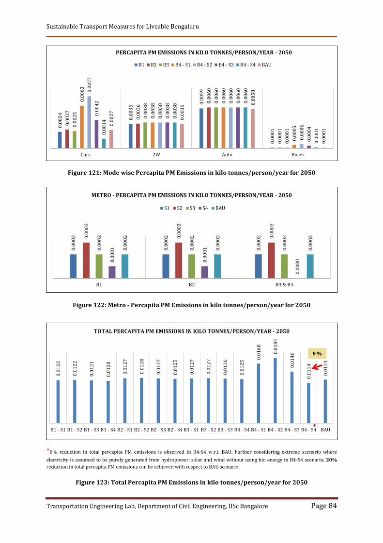
Sustainable Transport Measures for Liveable Bengaluru
Transportation Engineering Lab, Department of Civil Engineering, IISc Bangalore Page 84
Figure 121: Mode wise Percapita PM Emissions in kilo tonnes/person/year for 2050
Figure 122: Metro - Percapita PM Emissions in kilo tonnes/person/year for 2050
*8% reduction in total percapita PM emissions is observed in B4-S4 w.r.t. BAU. Further considering extreme scenario where
electricity is assumed to be purely generated from hydropower, solar and wind without using bio energy in B4-S4 scenario, 20%
reduction in total percapita PM emissions can be achieved with respect to BAU scenario
Figure 123: Total Percapita PM Emissions in kilo tonnes/person/year for 2050
0.0
02
4
0.0
03
6
0.0
05
9
0.0
00
1
0.0
02
7
0.0
03
6
0.0
06
0
0.0
00
1
0.0
02
5
0.0
03
8 0.0
06
0
0.0
00
1
0.0
06
3
0.0
03
8 0.0
06
0
0.0
00
5
0.0
07
7
0.0
03
8 0.0
06
0
0.0
00
6
0.0
04
2
0.0
03
8 0.0
06
0
0.0
00
4
0.0
01
4
0.0
03
8 0.0
06
0
0.0
00
1
0.0
02
7
0.0
03
6 0.0
05
8
0.0
00
1
Cars 2W Auto Buses
PERCAPITA PM EMISSIONS IN KILO TONNES/PERSON/YEAR - 2050
B1 B2 B3 B4 - S1 B4 - S2 B4 - S3 B4 - S4 BAU
0.0
00
2
0.0
00
2
0.0
00
20.0
00
3
0.0
00
3
0.0
00
3
0.0
00
2
0.0
00
2
0.0
00
2
0.0
00
1
0.0
00
1
0.0
00
0
0.0
00
2
0.0
00
2
0.0
00
2
B1 B2 B3 & B4
METRO - PERCAPITA PM EMISSIONS IN KILO TONNES/PERSON/YEAR - 2050
S1 S2 S3 S4 BAU
0.0
12
2
0.0
12
2
0.0
12
1
0.0
12
0
0.0
12
7
0.0
12
8
0.0
12
7
0.0
12
5
0.0
12
7
0.0
12
7
0.0
12
6
0.0
12
5
0.0
16
8
0.0
18
4
0.0
14
6
0.0
11
4
0.0
12
3
B1 - S1 B1 - S2 B1 - S3 B1 - S4 B2 - S1 B2 - S2 B2 - S3 B2 - S4 B3 - S1 B3 - S2 B3 - S3 B3 - S4 B4 - S1 B4 - S2 B4 - S3 B4 - S4 BAU
TOTAL PERCAPITA PM EMISSIONS IN KILO TONNES/PERSON/YEAR - 2050
8 %
*

Sustainable Transport Measures for Liveable Bengaluru
Transportation Engineering Lab, Department of Civil Engineering, IISc Bangalore Page 85
From the above figures it is clearly observed that Bundle 4 with scenario 4 is giving best
emission reduction because of 100% electrification from renewable sources of energy.
The total emissions values of Mass transportation systems like metro and bus may seem
higher but when the emissions are converted to percapita emissions, their share is quite
low due to high occupancy. Also, if the electricity generated from renewable sources is
coming exclusively from wind, hydel and solar and ‘NO BIO WASTE’ included then the
emissions reduces by a great amount.
5.11 RESULTS AND DISCUSSIONS
• Bundle 3 (bundle 4) which is a Combination of Planning, Regulatory & Economic
Instruments showed the maximum reduction in VKT in comparison to BAU for
2030 & 2050.
• Adding technological policy instruments further reduced emissions by a great
level as seen in Bundle 4.
• Total CO2 emissions in Bundle 3 are higher than B1 & B2 due to large mode shift
towards Public Transport while the Percapita emissions seems to be reducing due
to the same mode shift.
• For the horizon year 2030 and 2050 Bundle 4 - Scenario 4 showed the maximum
reduction of total emissions for all the pollutants CO, HC, NOx, CO2 and PM
respectively
• The total emissions of CO, HC, NOx and PM are showing almost 70% reduction in
emission with the implementation of B4-S4 scenario whereas 98% reduction can
be achieved in CO2 emissions.
• Total percapita NOx values in 2050 are higher in Bundle 4 for scenario 4 because
of the higher NOx values from electric cars compared to conventional cars. Since,
there is a shift towards public transportation the percapita emissions from cars
seems to be higher.
• Electrification of vehicles does more BAD than GOOD if electricity is generated
from non-renewable power sources. Nonrenewable power sources involve in high
PM, NOx and CO values which leads to higher emissions.
• If electricity is assumed to be purely generated from hydropower, solar and wind
without using bio energy in B4-S4 scenario,
• 73% reduction in total CO emissions and 26% reduction in percapita CO
emissions can be achieved with respect to BAU 2030 where, 77% reduction
in total CO emissions and 22% reduction in percapita CO emissions can be
achieved with respect to BAU 2050
• 99% reduction in total NOx emissions and 44% reduction in percapita
NOx emissions can be achieved with respect to BAU 2030 where, 98%

Sustainable Transport Measures for Liveable Bengaluru
Transportation Engineering Lab, Department of Civil Engineering, IISc Bangalore Page 86
reduction in total NOx emissions and 13% reduction in percapita NOx
emissions can be achieved with respect to BAU 2050
• 97% & 98% reduction in total PM emissions and 15% & 20% reduction
in percapita PM emissions can be achieved with respect to BAU scenario.

Sustainable Transport Measures for Liveable Bengaluru
Transportation Engineering Lab, Department of Civil Engineering, IISc Bangalore Page 87
6 CARBON EMISSION INTENSITY ESTIMATION FOR
TRANSPORT SECTOR MITIGATION POLICY BUNDLES
6.1 INTRODUCTION
In the international negotiations summit held at Paris in 2015 under the UNFCCC to tackle
the global issue of climate change, India declared a voluntary goal as a part of its Intended
Nationally Determined Contributions to reduce the emissions intensity of its GDP by 33 -
35% by 2030 from 2005 level. However, the INDC did not state the percentage share of
emission intensity reduction from transport sector, hence the same intended emission
intensity reduction percentage is assumed for transport sector. Emissions intensity is the
level of GHG emissions per unit of economic activity. It is generally calculated by
calculating the volume of emissions per unit of GDP.
In this report, we have forecasted the economic growth of Bangalore Metropolitan Region
(BMR). We have also estimated the reduction in emission intensity for the horizon years
from the base year due to the reduction in emissions resulting from the mitigation policy
scenarios in transport sector for BMR.
6.2 PAST TREND OF GDP IN INDIA
India is one of the fast growing economies of the world. India has highly conducive
environment because of the demographic advantage and increasing incomes to continue
on the path of a faster economic growth (Economic Survey of India 2016-17). The
following figure 124 shows the trend of Gross Domestic Product for all India at 2004-05
constant prices.
Figure 124: Past trend of GDP of India (in Rs. Crore at 2004-05 constant prices)
0
1000000
2000000
3000000
4000000
5000000
6000000
2005-06 2006-07 2007-08 2008-09 2009-10 2010-11 2011-12 2012-13
GD
P o
f In
dia
(R
s. C
rore
)

Sustainable Transport Measures for Liveable Bengaluru
Transportation Engineering Lab, Department of Civil Engineering, IISc Bangalore Page 88
Table 34: GDP and Growth Rate of India
Year GDP (Rs. Crore) All-India
At Constant Prices India Growth Rate
2005-06 3253073
2006-07 3564364 9.57%
2007-08 3896636 9.32%
2008-09 4158676 6.72%
2009-10 4516071 8.59%
2010-11 4918533 8.91%
2011-12 5247530 6.69%
2012-13 5482111 4.47%
GR (2005-13) 7.75%
CAGR (2005-13) 7.74%
6.3 PAST TREND OF GDDP FOR BENGALURU METROPOLITAN REGION
According to the report State and District Domestic Product of Karnataka by Directorate
of Economics and Statistics, Bengaluru the annual average growth rate of GDDP and
percapita GDDP for Bengaluru Urban, Bengaluru Rural and Ramanagaram were used and
the compound annual growth rate of GDDP and percapita GDDP for the period 2005-06
to 2012-13 at 2004-05 constant prices is estimated to be 9.25 % and 12.7% respectively.
The distribution of GDDP and percapita GDDP is given in the table 35 and table 36.
Table 35: CAGR of GDDP within BMR
Year GDDP (Rs. Crore) BMR At Constant Prices BMR Growth Rate (%)
2005-06 60561.00
2006-07 68939.45 13.83
2007-08 84325.97 22.32
2008-09 93390.43 10.75
2009-10 94705.27 1.41
2010-11 98907.90 4.44
2011-12 108459.81 9.66
2012-13 112522.24 3.75
GR (2005-13) 9.45
CAGR (2005-13) 9.25

Sustainable Transport Measures for Liveable Bengaluru
Transportation Engineering Lab, Department of Civil Engineering, IISc Bangalore Page 89
Table 36: CAGR of Percapita GDDP within BMR
Year Percapita GDDP (Rs. Crore) BMR
At Constant Prices BMR Growth Rate (%)
2005-06 1118.76
2006-07 1260.4 12.66
2007-08 1911.45 51.65
2008-09 2095.59 9.63
2009-10 2196.44 4.81
2010-11 2356.74 7.30
2011-12 2472.57 4.91
2012-13 2586.15 4.59
GR (2005-13) 13.65
CAGR (2005-13) 12.72
6.4 COMPARISON OF GDP OF INDIA AND GDDP OF BMR
The relation between the annual average growth rate of the GDP of India and the annual
average growth rate GDDP and percapita GDDP of BMR for the years 2005-13 at 2004-05
constant prices is established in the following table 37. The ratio factor of 1.20 between
the growth of BMR and the growth of India for years 2005-13 is observed.
Table 37: Relation Between the Growth of BMR and the Growth of India
Region
India
GDP
BMR
GDDP
BMR GR: India GR
(GDP)
Percapita BMR
GDDP
BMR GR: India GR
(percapita GDP)
CAGR (2005-13) 7.74 9.25 1.20 12.7 1.64
6.5 FORECAST OF GDP OF INDIA AND GDDP OF BMR
Various international organizations like OECD, PwC, World Bank and ADB have tried to
estimate the economic growth of India in future considering numerous national and
international factors. However only 2 organizations OECD and PwC have tried to forecast
India’s growth till 2050. For this study we will use the estimates as per the PwC forecast
which predicts the annual average growth rate of India for future time periods as
mentioned in the table 38. We have already calculated the ratio of growth rate of India to
the growth rate of BMR in the table 37. We use the same ratio for estimating the average
annual growth of GDDP of BMR for future time periods.

Sustainable Transport Measures for Liveable Bengaluru
Transportation Engineering Lab, Department of Civil Engineering, IISc Bangalore Page 90
Table 38: Estimation of GDDP and Percapita GDDP Growth Rate for BMR
Year Future Growth
projections for
India by PwC
Ratio of Growth
India Vs. BMR
(2005-13)
Estimated
GDDP Growth
rate for BMR
Ratio of percapita
Growth India Vs.
BMR
(2005-13)
Estimated
percapita GDDP
Growth rate for
BMR
2016 - 2020 7.80% 1.2 9.36% 1.64 12.79%
2021 - 2030 5.00% 1.2 6.00% 1.64 8.20%
2031 - 2040 4.40% 1.2 5.28% 1.64 7.22%
2041 - 2050 3.90% 1.2 4.68% 1.64 6.40%
Using the estimated GDDP growth rate for BMR for different decades till 2050, table 38
shows the estimated GDDP of BMR till horizon year 2050 in Rs. Crores at 2004-05
constant prices.
Figure 125: GDDP of BMR till 2050 (in Rs. Crore at 2004-05 constant prices)
Table 39: GDDP of BMR for horizon years
Year GDDP of BMR in Rs. Cr (at 2004-05 constant prices)
Base Year 93390
2030 412254
2050 1089585
0
200000
400000
600000
800000
1000000
1200000
20
10
20
12
20
14
20
16
20
18
20
20
20
22
20
24
20
26
20
28
20
30
20
32
20
34
20
36
20
38
20
40
20
42
20
44
20
46
20
48
20
50
BM
R G
DD
P (
in R
s. C
rore
)
Year

Sustainable Transport Measures for Liveable Bengaluru
Transportation Engineering Lab, Department of Civil Engineering, IISc Bangalore Page 91
Figure 126: GDDP of BMR till 2050 (in Rs. Crore at 2004-05 constant prices)
Table 40: Percapita GDDP of BMR for horizon years
Year Percapita GDDP of BMR in Rs. Cr (at 2004-05 constant prices)
Base Year 2096
2030 14897
2050 55624
6.6 EMISSION INTENSITY FROM TRANSPORT SECTOR
In earlier work packages, we have modelled the emissions from the transport sector in
the Business as Usual (BAU) scenario for base year and horizon years 2030 and 2050 for
Bangalore Metropolitan Region (BMR) along with the alternate sustainable transport
policy scenarios. The base year total CO2 has been estimated as 695617 tonnes/year. The
emission levels of CO2 and other local pollutants due to transportation sector have also
been estimated in this study. The estimated CO2 emissions are used to calculate the
emission intensity of transportation sector of BMR.
0
10000
20000
30000
40000
50000
60000
20
10
20
12
20
14
20
16
20
18
20
20
20
22
20
24
20
26
20
28
20
30
20
32
20
34
20
36
20
38
20
40
20
42
20
44
20
46
20
48
20
50B
MR
Pe
rca
pit
a G
DD
P (
in R
s. C
rore
)
Year

Sustainable Transport Measures for Liveable Bengaluru
Transportation Engineering Lab, Department of Civil Engineering, IISc Bangalore Page 92
Figure 127: Total CO2 emissions under BAU and policy scenarios for 2030
Figure 128: Total CO2 emissions under BAU and policy scenarios for 2050
GHG Emission Intensity = 𝐶𝑂2 𝐸𝑚𝑖𝑠𝑠𝑖𝑜𝑛𝑠
𝐺𝐷𝑃
Figures 127 and 128 shows GHG emission for the horizon year. Figures 129 and 131
displays the GHG emission intensity calculated under various mitigation policy scenarios
for the horizon years 2030 and 2050.
16
70
97
21
21
49
09
12
11
64
87
04
18
06
49
6
17
11
09
48
19
75
80
40
11
91
03
17
17
96
60
0
18
46
53
58
23
80
71
04
12
81
09
81
18
14
85
9
18
92
79
30
24
91
17
99
12
59
38
51
27
58
98
16
78
27
59
B1 - S1 B1 - S2 B1 - S3 B1 - S4 B2 - S1 B2 - S2 B2 - S3 B2 - S4B3 - S1 B3 - S2 B3 - S3 B3 - S4 B4 - S1 B4 - S2 B4 - S3 B4 - S4 BAU
TOTAL CO2 EMISSIONS IN TONNES/YEAR - 20301
74
43
42
2
22
57
05
25
12
80
62
58
30
41
97
9
17
57
37
53
22
76
41
54
12
87
93
40
29
94
51
5
17
74
67
79
23
00
04
77
12
99
51
17
29
89
74
5
18
89
31
61
25
50
85
31
12
90
99
43
31
13
04
17
66
24
78
B1 - S1 B1 - S2 B1 - S3 B1 - S4 B2 - S1 B2 - S2 B2 - S3 B2 - S4B3 - S1 B3 - S2 B3 - S3 B3 - S4 B4 - S1 B4 - S2 B4 - S3 B4 - S4 BAU
TOTAL CO2 EMISSIONS IN TONNES/YEAR - 2050

Sustainable Transport Measures for Liveable Bengaluru
Transportation Engineering Lab, Department of Civil Engineering, IISc Bangalore Page 93
Figure 129: GHG Emission intensity under BAU and alternate policy scenarios for 2030
*The carbon emissions intensity is increasing at the greater rate in BAU 2030 scenario because Metro is not available in Bengaluru
during base year and it is the only electricity based transportation with high emission factor values. Further, assuming electricity will be purely generated from hydropower, solar and wind without using bio energy in BAU scenario, 39% reduction in total CO2 emission intensity can be achieved in BAU 2030 with respect to base year
Figure 130: Reduction in Emission intensity under BAU and alternate policy scenarios for 2030
Figure 131: GHG Emission intensity under BAU and alternate policy scenarios for 2050
40
.53 52
.13
28
.26
4.3
8
41
.51
47
.93
28
.89
4.3
6
44
.79 5
7.7
5
31
.08
4.4
0
45
.91 6
0.4
3
30
.55
0.6
7
40
.71
B1 - S1 B1 - S2 B1 - S3 B1 - S4 B2 - S1 B2 - S2 B2 - S3 B2 - S4B3 - S1 B3 - S2 B3 - S3 B3 - S4 B4 - S1 B4 - S2 B4 - S3 B4 - S4 BAU
EMISSION INTENSITY (TONNES OF CO2/RS. CRORE) FOR 20301
6.0
1
20
.71
11
.75
2.7
9
16
.13
20
.89
11
.82
2.7
5
16
.29
21
.11
11
.93
2.7
4
17
.34
23
.41
11
.85
0.2
9
16
.21
B1 - S1 B1 - S2 B1 - S3 B1 - S4 B2 - S1 B2 - S2 B2 - S3 B2 - S4B3 - S1 B3 - S2 B3 - S3 B3 - S4 B4 - S1 B4 - S2 B4 - S3 B4 - S4 BAU
EMISSION INTENSITY (TONNES OF CO2/RS. CRORE) FOR 2050
44
4%
60
0%
27
9%
-41
%
45
7% 54
3%
28
8%
-41
%
50
1%
67
5%
31
7%
-41
%
51
6%
71
1%
31
0%
-91
%
44
7%
B1 - S1 B1 - S2 B1 - S3 B1 - S4 B2 - S1 B2 - S2 B2 - S3 B2 - S4B3 - S1 B3 - S2 B3 - S3 B3 - S4 B4 - S1 B4 - S2 B4 - S3 B4 - S4 BAU
REDUCTION IN EMISSION INTENSITY FROM BASE YEAR FOR 2030
*

Sustainable Transport Measures for Liveable Bengaluru
Transportation Engineering Lab, Department of Civil Engineering, IISc Bangalore Page 94
* The carbon emissions intensity is increasing at the greater rate in BAU 2050 scenario because Metro is not available in Bengaluru
during base year and it is the only electricity based transportation with high emission factor values. Further, assuming electricity is
purely generated from hydropower, solar and wind without using bio energy in BAU scenario, 60% reduction in total CO2 emission
intensity can be achieved in BAU 2050 with respect to base year.
Figure 132: Reduction in Emission intensity under BAU and alternate policy scenarios for 2050
The percentage reduction in GHG emission intensity of the transport sector of BMR in the
horizon years 2030 and 2050 from the base year under BAU and alternate mitigation
policy scenarios is demonstrated in the figure 130 and figure 132. The total percapita CO2
emissions for base year is estimated as 242 kilo tonnes/person/year.
Figure 133: Total Percapita CO2 Emissions under BAU and alternate policy scenarios for 2030
22
5.3
63
0
22
7.1
48
5
22
3.4
73
1
21
9.7
97
7
22
3.3
96
8
22
4.3
79
8
22
1.4
65
5
21
7.7
09
7
22
6.4
61
1
22
8.3
80
8
22
4.4
29
0
22
0.4
77
2
19
3.1
01
4
22
3.0
33
4
16
1.4
12
6
99
.78
36
22
8.8
91
8
B1 - S1 B1 - S2 B1 - S3 B1 - S4 B2 - S1 B2 - S2 B2 - S3 B2 - S4B3 - S1 B3 - S2 B3 - S3 B3 - S4 B4 - S1 B4 - S2 B4 - S3 B4 - S4 BAU
TOTAL PERCAPITA CO2 EMISSIONS IN KILO TONNES/PERSON/YEAR - 2030
11
5%
17
8%
58
%
-63
%
11
7%
18
0%
59
%
-63
%
11
9%
18
3%
60
%
-63
%
13
3%
21
4%
59
%
-96
%
11
8%
B1 - S1 B1 - S2 B1 - S3 B1 - S4 B2 - S1 B2 - S2 B2 - S3 B2 - S4B3 - S1 B3 - S2 B3 - S3 B3 - S4 B4 - S1 B4 - S2 B4 - S3 B4 - S4 BAU
REDUCTION IN EMISSION INTENSITY FROM BASE YEAR FOR 2050
*

Sustainable Transport Measures for Liveable Bengaluru
Transportation Engineering Lab, Department of Civil Engineering, IISc Bangalore Page 95
Figure 134: Total Percapita CO2 Emissions under BAU and alternate policy scenarios for 2050
Figure 133 and figure 134 shows the percapita GHG emission intensity calculated under
various mitigation policy scenarios for the horizon years 2030 and 2050.
Figure 135: Percapita GHG Emissions intensity under BAU and alternate policy scenarios for 2030
*Assuming electricity is purely generated from hydropower, solar and wind without using bio energy in BAU scenario, 87% reduction
in total percapita CO2 emission intensity can be achieved in BAU 2030with respect to base year.
Figure 136: Percentage reduction in Percapita GHG emission intensity of the transport sector of
BMR for 2030
18
1.8
68
2
18
2.6
98
3
18
1.1
17
3
17
9.5
36
4
18
2.4
93
5
18
3.3
26
5
18
1.7
40
1
18
0.1
53
7
18
6.7
46
0
18
7.5
63
9
18
6.0
06
2
18
4.4
48
5
14
7.1
87
0
17
1.6
92
7
12
5.0
16
3
78
.34
69
17
7.7
76
7
B1 - S1 B1 - S2 B1 - S3 B1 - S4 B2 - S1 B2 - S2 B2 - S3 B2 - S4B3 - S1 B3 - S2 B3 - S3 B3 - S4 B4 - S1 B4 - S2 B4 - S3 B4 - S4 BAU
TOTAL PERCAPITA CO2 EMISSIONS IN KILO TONNES/PERSON/YEAR - 20500
.01
51
0.0
15
2
0.0
15
0
0.0
14
8
0.0
15
0
0.0
15
1
0.0
14
9
0.0
14
6
0.0
15
2
0.0
15
3
0.0
15
1
0.0
14
8
0.0
13
0
0.0
15
0
0.0
10
8
0.0
06
7
0.0
15
4
B1 - S1 B1 - S2 B1 - S3 B1 - S4 B2 - S1 B2 - S2 B2 - S3 B2 - S4B3 - S1 B3 - S2 B3 - S3 B3 - S4 B4 - S1 B4 - S2 B4 - S3 B4 - S4 BAU
PER-CAPITA EMISSION INTENSITY (KILO TONNES OF CO2/RS. CRORE/PERSON) FOR 2030
86
.88
%
86
.78
%
86
.99
%
87
.21
%
87
.00
%
86
.94
%
87
.11
%
87
.33
%
86
.82
%
86
.71
%
86
.94
%
87
.17
%
88
.76
%
87
.02
% 90
.61
% 94
.19
%
86
.68
%
B1 - S1 B1 - S2 B1 - S3 B1 - S4 B2 - S1 B2 - S2 B2 - S3 B2 - S4B3 - S1 B3 - S2 B3 - S3 B3 - S4 B4 - S1 B4 - S2 B4 - S3 B4 - S4 BAU
REDUCTION IN PER-CAPITA EMISSION INTENSITY FROM BASE YEAR FOR 2030
*

Sustainable Transport Measures for Liveable Bengaluru
Transportation Engineering Lab, Department of Civil Engineering, IISc Bangalore Page 96
Figure 137: Percapita GHG Emissions intensity under BAU and alternate policy scenarios for 2050
*Assuming electricity is purely generated from hydropower, solar and wind without using bio energy in BAU scenario, 97% reduction
in total percapita CO2 emission intensity can be achieved in BAU 2050 with respect to base year.
Figure 138: Percentage reduction in Percapita GHG emission intensity of the transport sector of
BMR for 2050
The percentage reduction in percapita GHG emission intensity of the transport sector of
BMR in the horizon years 2030 and 2050 from the base year under BAU and alternate
mitigation policy scenarios is displayed in figure 135 and figure 137. The carbon
emissions intensity is increasing at the greater rate in BAU 2030 scenario because Metro
is not available in Bengaluru during base year and it is the only electricity based
transportation with high emission factor values. The share of generation of electricity
from renewable and non-renewable sources plays a significant role in emission intensity.
The study clearly states that the emission reduction reaches the INDC targets even for the
BAU scenarios of 2030 and 2050 with the extreme scenario case of assuming that the
electricity will be purely generated from renewable sources. The substantial reduction in
emission intensity of the transportation sector of 91% and 96%is observed for the
horizon year 2030 and 2050 respectively under the BAU and the best mitigation policy
scenario of Bundle 4-Scenario 4. Similarly, up to 98% reduction in percapita emission
intensity has been observed for the horizon year 2050.
0.0
03
27
0.0
03
28
0.0
03
26
0.0
03
23
0.0
03
28
0.0
03
30
0.0
03
27
0.0
03
24
0.0
03
36
0.0
03
37
0.0
03
34
0.0
03
32
0.0
02
65
0.0
03
09
0.0
02
25
0.0
01
41
0.0
03
20
B1 - S1 B1 - S2 B1 - S3 B1 - S4 B2 - S1 B2 - S2 B2 - S3 B2 - S4B3 - S1 B3 - S2 B3 - S3 B3 - S4 B4 - S1 B4 - S2 B4 - S3 B4 - S4 BAU
PER-CAPITA EMISSION INTENSITY (KILO TONNES OF CO2/RS. CRORE/PERSON) FOR 2050
97
.17
%
97
.15
%
97
.18
%
97
.20
%
97
.16
%
97
.14
%
97
.17
%
97
.19
%
97
.09
%
97
.08
%
97
.10
%
97
.13
% 97
.71
%
97
.32
% 98
.05
% 98
.78
%
97
.23
%
B1 - S1 B1 - S2 B1 - S3 B1 - S4 B2 - S1 B2 - S2 B2 - S3 B2 - S4B3 - S1 B3 - S2 B3 - S3 B3 - S4 B4 - S1 B4 - S2 B4 - S3 B4 - S4 BAU
Reduction in Per-capita Emission Intensity from Base Year for 2050
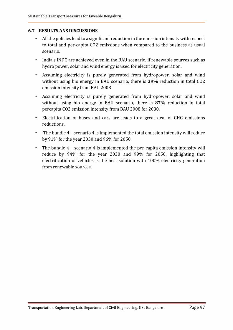
Sustainable Transport Measures for Liveable Bengaluru
Transportation Engineering Lab, Department of Civil Engineering, IISc Bangalore Page 97
6.7 RESULTS ANS DISCUSSIONS
• All the policies lead to a significant reduction in the emission intensity with respect
to total and per-capita CO2 emissions when compared to the business as usual
scenario.
• India’s INDC are achieved even in the BAU scenario, if renewable sources such as
hydro power, solar and wind energy is used for electricity generation.
• Assuming electricity is purely generated from hydropower, solar and wind
without using bio energy in BAU scenario, there is 39% reduction in total CO2
emission intensity from BAU 2008
• Assuming electricity is purely generated from hydropower, solar and wind
without using bio energy in BAU scenario, there is 87% reduction in total
percapita CO2 emission intensity from BAU 2008 for 2030.
• Electrification of buses and cars are leads to a great deal of GHG emissions
reductions.
• The bundle 4 – scenario 4 is implemented the total emission intensity will reduce
by 91% for the year 2030 and 96% for 2050.
• The bundle 4 – scenario 4 is implemented the per-capita emission intensity will
reduce by 94% for the year 2030 and 99% for 2050, highlighting that
electrification of vehicles is the best solution with 100% electricity generation
from renewable sources.

Sustainable Transport Measures for Liveable Bengaluru
Transportation Engineering Lab, Department of Civil Engineering, IISc Bangalore Page 98
7 CONSUMER SURPLUS CALCULATIONS FOR
EVALUATED POLICY BUNDLES BANGALORE
7.1 INTRODUCTION
Consumer surplus is defined as the difference between the consumers’ willingness to pay
in terms of travel costs (travel time, etc.) and what they actually pay is called consumer
surplus.
Calculation of consumer surplus using rule of half: The rule of one-half estimates the
change in consumer surplus for small changes in supply with a constant demand curve.
Figure 139: Change in Consumer Surplus
When price of travel changes from Pij0 to Pij1 demand changes from Dij0 to Dij1 as
illustrated in the figure. Then the change in consumer surplus (user’s benefit or costs)
due to a change is equal to the area of the triangle ABC.
7.2 CALCULATION OF CONSUMER SURPLUS
7.2.1 Private Transport
Consumer surplus for year 2030 and 2050 for each of the vehicle types that share road
network will be calculated according to the following:
1 0 1 0 1 0 1 1 0 0
2030 1/ 2 ( ) ( ) 1/ 2 ( ) ( C C )M M M M M M M M M M M M
ij ij ij ij ij ij ij ij
i I j J i I j J
CS VoT D D T T D D F Dist F Dist
Where, M modes that use road network
VoT is value of travel time for mode M, Rupee/minutes
D is travel demand for mode M
T is travel time for mode M in minute
Dist is travel distance for mode M in km
FC is fuel cost, Rupee/ km

Sustainable Transport Measures for Liveable Bengaluru
Transportation Engineering Lab, Department of Civil Engineering, IISc Bangalore Page 99
7.2.2 Public Transport
For public transport mode the calculation will be made according to the following
1 0 1 0
2030 1/ 2 ( ) ( )PT PT PT PT PT PT
ij ij ij ij
i I j J
CS VoT D D T T
Where, PT stands for public transport
VoT is value of travel time for public transport
D is travel demand for public transport
T is total travel time for public transport
The fuel cost is calculated by making a shortest path assignment for a distance matrix.
The distance matrix multiplied by mode specific fuel cost is travel cost related to fuel
cost.
Parking costs have been added wherever it is applicable once the fuel cost matrix is
carried.
Congestion pricing is multiplied with the distance travelled wherever applicable and
added to the total costs.
7.3 VALUE OF TIME
Value of Travel Time (VOT)-Traveller’s value of time can be estimated from the degree to
which they are either willing to pay money to save travel time or incur extra travel time
to save money.
Table 41: Value of Time adopted for the study
Mode VOT/hr VOT/min
Taxi 54 0.9
Auto rickshaw 36 0.6
Two wheeler 25.8 0.43
Car/Van 63 1.05
Bus 14.4 0.24
Metro 14.4 0.24
(Source: Comprehensive traffic and transportation study, Bangalore 2010)
The CTTS report doesn’t provide the VOT values for Metro and NMT. Considering metro
is a public transportation mode, VOT which is used for Bus is adopted for metro. This
report doesn’t consist the consumer surplus values of NMT due to the unavailability of
VOT.

Sustainable Transport Measures for Liveable Bengaluru
Transportation Engineering Lab, Department of Civil Engineering, IISc Bangalore Page 100
7.4 EVALUATED POLICY BUNDLES AND CONSUMER SURPLUS
7.4.1 Policy Bundle 1
The policies in the policy bundle 1 are listed below:
a. Increasing network of public transit
b. Cycling and Walking Infrastructure
c. Additional taxes on new vehicle purchase
By implementing this policy bundle there has been a shift in the mode share from private
mode to public transportation. Since the VOT is considered as 1 all the consumer surplus
values will be defined in terms of money saved or money lost.
Figure 140 shows the consumer surplus values by implementing the policy bundle 1. It is
found that the 2wheelers are losing more money compared to other modes. The
consumer surplus values for public transport modes like bus and metro are positive
which signifies that they are saving money by using that mode.
Figure 140: CS values for policy bundle 1 (Money saved/lost)
7.4.2 Policy Bundle 2
The policies in the policy bundle 2 are as follows:
a. Additional taxes on new vehicle purchase
b. Strict Vehicles inspection/ Improvement in standards for vehicle emission
c. Increase in fuel cost
This bundle aim is to increase the operating costs of private vehicles. By implementing
this bundle, it was found that there is a shift from private mode to public transport. Figure
141 shows the consumer surplus for the various modes upon implementing bundle 2.
-49259455
-208084265
-8036267
34671028590
-407060734
-759578240
-91761929
590952 68586
Car 2W Auto Bus Metro
CS VALUES FOR POLICY BUNDLE 1 IN INR (MONEY SAVED/LOST)
2030 2050

Sustainable Transport Measures for Liveable Bengaluru
Transportation Engineering Lab, Department of Civil Engineering, IISc Bangalore Page 101
Figure 141: CS values for policy bundle 2 (Money saved/lost)
7.4.3 Bundle 3
The policies in the policy bundle 3 are listed below:
a. Increasing network coverage of Public Transit
b. Defining car restricted zones
c. Congestion Pricing
d. Park and Ride
e. Cycling and Walking infrastructure
f. Encouraging car-pooling and High Occupancy Lanes
g. High density mix building use along main transport corridors
This bundle concentrates on providing proper network coverage for public transport,
increasing the operation costs for private vehicles and providing proper infrastructure
for mass transport and non-motorized transport. It is observed that this bundle is
efficient in reducing the emissions because of the considerable shift from private to public
transport.
Figure 142 shows the consumer surplus values obtained by implementing this policy
bundle. As mentioned earlier negative sign signifies losing money by using that particular
mode. It is observed that 2 wheelers loose more in this case as well. This is because of the
shift in the mode of transport upon the bundle implementation.
-61804398
-269182227
-16157881
366971 32185
-454277860
-943991513
-183750217
701812 81488
Car 2W Auto Bus Metro
CS VALUES FOR POLICY BUNDLE 2 IN INR (MONEY SAVED/LOST)
2030 2050

Sustainable Transport Measures for Liveable Bengaluru
Transportation Engineering Lab, Department of Civil Engineering, IISc Bangalore Page 102
Figure 142: CS values for policy bundle 3 (Money saved/lost)
7.5 SUMMARY
Consumer surplus costs associated with bundles 1, 2 & 3 have been estimated and it was
found that Bundle 3 consumers who use Public transportation gain about Rs. 0.71
million/day in the year 2030 and Rs. 1.1 million/day in 2050 while the 2 wheeler users
are at the major loss with Rs. 360 million/day in 2030 and Rs. 1220 million/day in 2050.
The reason for high consumer surplus values for two wheeler and auto rickshaw could
be because of the mode shift between BAU and policy bundles. Added to that, the private
vehicle formula above also includes fuel costs as well which further increases their value.
-74353573
-360659398
-29664629
653050 53592
-517723778
-1220462688
-236414507
965585 126743
Car 2W Auto Bus Metro
CS VALUES FOR POLICY BUNDLE 3 IN INR (MONEY SAVED/LOST)
2030 2050

Sustainable Transport Measures for Liveable Bengaluru
Transportation Engineering Lab, Department of Civil Engineering, IISc Bangalore Page 103
8 ADAPTATION POLICY BUNDLES FOR
TRANSPORTATION SECTOR
8.1 INTRODUCTION
Urban floods are the main focus for the adaptation part of the project and so most of the
policies have been formulated keeping urban flooding in mind. Climate change is
inevitable; however, adaptive strategies help in strengthening the road network system
act as resilient measures against urban floods. Figure 143 shows the sequential steps
followed in Policy formulation for Adaptation.
Model outcome Identify the links used
most frequently
Overlaying the outcome of the model with flood maps to identify
the vulnerable links in the transport system
Flood Maps
To study the characteristics (land use, type of road, capacity of the road v/s the volume, material of the road, presence of storm water drains on the road)
of the identified vulnerable links
Evaluating adaptation policies as per the characteristics of the
vulnerable links
Figure 143: Policies Formulation for Adaptation Flow Chart
Start
Finalizing the best bundle for Adaptation
End
Estimation of evaluation parameters

Sustainable Transport Measures for Liveable Bengaluru
Transportation Engineering Lab, Department of Civil Engineering, IISc Bangalore Page 104
8.2 BUSINESS AS USUAL SCENARIO
Bangalore Metropolitan Region flood map is prepared based on the heavy rainfall
occurred on November 3rd 2015 (total rainfall - 266mm, duration - 4 hrs 10 mins, return
period – 100yrs).
Figure 144: DEM Map - BMR
Figure 145: Flood Map - BMR
For business as usual scenario we considered the base road network which was used for
mitigation. Flood map is overlaid over the road network to find out the vulnerable
locations. The road network showing the flood depth is presented in figure 145. For the
BAU network each road link is divided into multiple small links depending on the level of
flood in that particular link. The percentage share of flood depth on road network of BMR
is shown in Figure 147. Flooding reduces the vehicle speeds and the percentage change
in speed with flood depth is shown in table 42.
Table 42: Relation between Flood Depth and Travel Speed Reduction
FLOOD DEPTH (m) TRAVEL SPEED REDUCTION
0 - 0.1 No Change
0.1 - 0.2 0 - 25%
0.2 - 0.3 25% - 50%
0.3 - 0.5 50% - 75%
Above 0.5 75% - 99%
Road Closed
(Source: Pregnolato et al. 2016)

Sustainable Transport Measures for Liveable Bengaluru
Transportation Engineering Lab, Department of Civil Engineering, IISc Bangalore Page 105
Figure 146: Road network with flood level Map - BMR
For the BAU network each road link is divided into multiple small links depending on the
level of flood in that particular link. Links which carry a flood depth above than 0.5 m are
not considered in the BAU model. Roads that are heavily flooded and the zones that do
not have redundant roads for the trip to happen are considered to have no trips from
those zones. There are about 7 such zones in which the trips are cancelled.
Figure 147: Percentage Share of Flood Depth in Road Network
28
35
9
14
6
43 2
PERCENTAGE SHARE OF FLOOD DEPTH (%)
0-0.01
0.01-0.1
0.1-0.2
0.2-0.3
0.3-0.4
0.4-0.5
0.5-2
2.0-9.0
Depth (m)

Sustainable Transport Measures for Liveable Bengaluru
Transportation Engineering Lab, Department of Civil Engineering, IISc Bangalore Page 106
Bengaluru has about 180-200 km length of primary and secondary storm water
drainages and nothing was added in the BAU model. BAU modelling is done for the base
year and for the future years 2030, 2050 for both private and public transport networks.
Since this is not a frequent event and not a usual scenario the mode shift is kept the same
even though trip lengths change. Due to the flooding of roads, people who commute in
their usual shortest paths change their course which leads to longer paths and longer
travel time.
8.3 BAU ADAPTATION RESULTS
8.3.1 Comparison of Vehicle kilometres travelled
Vehicle kilometres travelled are compared between no flooding and flooding scenarios
for base year, 2030 & 2050.
Table 43: Comparison of VKT for BAU scenarios Base Year, 2030 and 2050
BAU- No Flooding
(VKT in millions) (km)
BAU- Flooding
(VKT in millions) (km)
Base Year 2030 2050 Base Year 2030 2050
PVT 28.69 39.3 55.8 29.6 41.2 57.2
PT 2.3 8.7 16.3 2.8 9.6 18.1
Total 30.99 48 72.1 32.4 50.8 75.3
Figure 148: Comparison of VKT for No Flooding and Flooding BAU scenarios - BAU
It is observed from the figure 148 that the vehicle kilometres travelled are increasing due
to the fact that the shortest paths are flooded and the commuters are taking another path
which is longer than the usual path.
30
.99
48
72
.1
32
.4
50
.8
75
.3
B A S E Y E A R 2 0 3 0 2 0 5 0
V K T I N M I L L I O N S ( K M ) - B A U
BAU - No Flooding BAU - Flooding
4 %
6 %
4 %

Sustainable Transport Measures for Liveable Bengaluru
Transportation Engineering Lab, Department of Civil Engineering, IISc Bangalore Page 107
8.3.2 Vehicle Hours Travelled
Due to flooding and blockage of roads people tend to use alternative routes which will be
longer than the usual paths which increase the travel times. The figure 149 illustrates the
comparison between vehicle Hours Travelled (VHT) for Non- flooding and flooding BAU
scenarios for base year, 2030 & 2050.
Figure 149: Comparison of VHT between BAU No flooding and BAU flooding scenarios – BAU
8.3.3 Average Travel Speeds
The relation between flood depth and speed clearly explains that as the level of flood
increases vehicle speeds decrease. Using this relation new vehicle speeds and travel times
are estimated which will then be fed in to model for assigning trips to the road network.
From the figure 150, it is evident that the average daily vehicle speed reduces from
27kmph in base year no flooding to 13kmph during flooding in 2050.
Figure 150: Comparison of Average Travel Speeds between BAU No Flooding and BAU Flooding
Scenario
27
.2
25
.4
23
.6
20
.2
16
.8
13
.2
B A S E Y E A R 2 0 3 0 2 0 5 0
A V G . V E H I C L E S P E E D S ( K M P H ) - B A U
BAU - No Flooding BAU - Flooding26 %
34 %44 %
5.5
9.5
16
.6
6.8
11
.3
19
B A S E Y E A R 2 0 3 0 2 0 5 0
V H T - B A U ( M I L H R S )
BAU - No Flooding BAU - Flooding
23 %
19 %
14 %

Sustainable Transport Measures for Liveable Bengaluru
Transportation Engineering Lab, Department of Civil Engineering, IISc Bangalore Page 108
8.3.4 Average Trip Lengths
It is observed from the figure 151, that the average private transport trip lengths increase
from14.1 km in BAU base year (no flood scenario) to 21.7 km in 2050 for a flood scenario.
For public transport the average trip lengths increase from 11.4 km in BAU base year no
flooding scenario to 20.4 km in 2050 flooding scenario.
Figure 151: Comparison of Avg. trip lengths for base year, 2030 and 2050 for Private and Public
Transport
8.3.5 Cancelled Trips
It is assumed that the zones which are flooded and have no access to other zones are
considered to have cancelled their trips. Table 44 shows the total trips cancelled due to
flooding for BAU scenario.
Table 44: Cancelled trips for BAU No flooding and BAU Flooding case for BAU
Cancelled Trips
BAU - No flooding BAU Flooding Total Trips
assigned % Trips
cancelled
0 160786 6 million 2.8
8.3.6 Trip Assignment Figures
The figures152 - 154 shows the flows on the BMR road network for the base year, 2030
& 2050 for private and public transport for BAU scenario.
14
.1 17
.4
18
.17
17
.9 20
.8
21
.7
B A S E Y E A R 2 0 3 0 2 0 5 0
A V E R A G E T R I P L E N G T H ( K M ) -P R I V A T E
BAU - No Flooding BAU - Flooding
27 % 19 %
19 %
11
.4
16
.36
17
.67
14
19
.2
20
.4
B A S E Y E A R 2 0 3 0 2 0 5 0
A V E R A G E T R I P L E N G T H ( K M ) -P U B L I C
BAU - No Flooding BAU - Flooding
23 %
17 %15 %

Sustainable Transport Measures for Liveable Bengaluru
Transportation Engineering Lab, Department of Civil Engineering, IISc Bangalore Page 109
Figure 152: Vehicle flows on BMR road network for base year for BAU flooding
Figure 153: Vehicle flows on BMR road network for 2030 for BAU flooding

Sustainable Transport Measures for Liveable Bengaluru
Transportation Engineering Lab, Department of Civil Engineering, IISc Bangalore Page 110
Figure 154: Vehicle flows on BMR road network for 2050 for BAU flooding
8.4 ADAPTATION POLICY BUNDLES
Adaptive measures are seen as a tool to reduce the vulnerability to the potential negative
impacts of climate change and strengthen the inherent capacity of a system to undertake
defensive as well as protective actions that help to avoid loss and facilitate recovery from
any impact by increasing the resilience of the entire system. The main objective of the
adaptation strategies is to create a transportation system that is resilient to urban
flooding.
Urban floods are the main focus for the adaptation part of the project and so most of the
policies have been formulated keeping urban flooding in mind. Climate change is
inevitable; however, adaptive strategies will help in strengthening the road network
system and act as resilient measures against urban floods. Bundles are formulated in such
a way that there is resilience in the infrastructure and also a reduction in runoff on the
road network. The policy bundles for adaptation are listed in the table 45.

Sustainable Transport Measures for Liveable Bengaluru
Transportation Engineering Lab, Department of Civil Engineering, IISc Bangalore Page 111
Table 45: Policy Bundles for Adaptation
Policy Bundles
BUNDLE 1
Replacement of impermeable road surface with permeable material in vulnerable areas
Slum relocation and rehabilitation
Providing proper drainage facilities at vulnerable areas
Construction of redundant infrastructure
BUNDLE 2
Rerouting people during flooding
Restricting development in low lying or vulnerable areas
Slum relocation and rehabilitation
BUNDLE 3
Replacement of impermeable surfaces with permeable material in vulnerable areas
Providing proper drainage facilities at vulnerable areas
Rerouting people during flooding
Each policy bundle has a certain number of policies amalgamated together to bring out
specific results after implementation. These sub-policies affect the travel demand
modelling at various stages. A particular policy from a policy bundle might have an
impact on more than one stage of the Travel Demand Model (TDM). In the following
sections, the above policies are discussed and the impact of the policies on the TDM is
explained for each policy bundle separately.

Sustainable Transport Measures for Liveable Bengaluru
Transportation Engineering Lab, Department of Civil Engineering, IISc Bangalore Page 112
8.5 POLICY BUNDLES AND THEIR IMPACT ON THE TDM
8.5.1 Policy Bundle 1
Figure 155: Impact of policy bundle 1 in Four stage modelling
Future productions & attractions
Start
Trip Distribution- OD Matrix & TLD
Multinomial Logit Mode choice model
In vehicle travel time, walking time to and from stops,
waiting time at stops, Fare charge,
parking cost etc Calculation of Utilities
log Likelihood
END
Future year Planning data (Future population, Future Employment)
Trip Assignment
Private Transport
Assignment
Public Transit
Assignment
Future private transport road
network
Private transport cost skim
Public transport cost skim
Public and Private VKT
Future PT road network
Replacement of impermeable road surface with permeable material in vulnerable areas Providing proper drainage facilities at vulnerable areas Construction of redundant infrastructure

Sustainable Transport Measures for Liveable Bengaluru
Transportation Engineering Lab, Department of Civil Engineering, IISc Bangalore Page 113
8.5.2 Policy Bundle 2
Figure 156: Impact of policy bundle 2 in Four stage modelling
Future productions & attractions
Start
Trip Distribution- OD Matrix & TLD
Multinomial Logit Mode choice model
In vehicle travel time, walking time to and from stops,
waiting time at stops, Fare charge,
parking cost etc Calculation of Utilities
log Likelihood
END
Future year Planning data (Future population, Future Employment)
Trip Assignment
Private Transport
Assignment
Public Transit Assignment
Future private transport road
network
Private transport cost skim
Public transport cost skim
Public and Private VKT
Future PT road network
Rerouting people during flooding

Sustainable Transport Measures for Liveable Bengaluru
Transportation Engineering Lab, Department of Civil Engineering, IISc Bangalore Page 114
8.5.3 Policy Bundle 3
Figure 157: Impact of policy bundle 3 in Four stage modelling
8.6 EVALUATION READY DESCRIPTION OF ADAPTATION POLICIES
The bundles mentioned in table 45 have some policies common across the bundles.
Evaluation of each of these policies is described below.
Future productions & attractions
Start
Trip Distribution- OD Matrix & TLD
Multinomial Logit Mode choice model
In vehicle travel time, walking time to and from stops,
waiting time at stops, Fare charge,
parking cost etc Calculation of Utilities
log Likelihood
END
Future year Planning data (Future population, Future Employment)
Trip Assignment
Private Transport
Assignment
Public Transit
Assignment
Future private transport road
network
Private transport cost skim
Public transport cost skim
Public and Private VKT
Future PT road network
Rerouting people during flooding

Sustainable Transport Measures for Liveable Bengaluru
Transportation Engineering Lab, Department of Civil Engineering, IISc Bangalore Page 115
8.6.1 Replacement of impermeable road surface with permeable material in
vulnerable areas
Most of the Bengaluru road networks have impermeable pavement systems. If there is
improper drainage system, then even less intense rainfall accumulates certain depth of
water on the surface of the pavement, thereby blocking the road, resulting higher vehicle
hours travelled and higher vehicle kilometres travelled. As a strategy to increase the
water permeation into the road, the above policy was adopted. It aims the replacement
of impermeable road surface by permeable material in the high flooding road networks.
Vulnerable links are identified depending on flood depth (above 0.3m), connectivity and
the policy is being suggested.
The replacement of impermeable to permeable reduces the runoff rates and growing
volumes of storm water collected in urbanised areas. Porous asphalt eliminates splash
and spray behind vehicles and avoid reflections from the surface of the pavement at both
day and night thus making road marks more visible. There is also a significant reduction
of evaporation.
This policy will have an impact on the Trip Assignment of the TDM. This is because if the
material of the roads in vulnerable sections gets replaced by permeable material then
flood depth will reduce and thus people will be able to travel at the same speed without
much variation, to their destinations.
The following variables are subject to change:
Cancelled Trips
Vehicle Hours Travelled (VHT)
Vehicle Kilometres Travelled (VKT)
Average Trip Length
According to literature, in comparison to conventional asphalts, permeable and porous
pavements provide effective peak flow reductions up to 42% and longer discharging
times. Thus keeping other parameters constant, the flood depth reduces by 42%. From
the assumption the range of flood depth (0.3m - 0.5m) was fixed and 25 vulnerable road
links that were selected for incorporating in the model is shown in table 46 and the map
depicting the identified location are given in figure 157. Table 46: Locations to implement the policy
1. Vivekananda Park Road 2. State Bank Road 3. Tannery Road 4. Ramakrishna Road 5. 1st Main (Prashanth Nagar Main
Road) 6. Elephant Cave Road
7. Temple Street 8. Main Guard Cross Road 9. C J Venkatesa Das Road 10. Bagalgunte Main Road 11. Byrasandra Main Road 12. JeevanBhima Nagar 10th Main
Road 13. Jeevanahalli Main Road 14. Nehru Road 15. Arumugam Circle 16. Annapoorneshwarinagar Main
Road 17. Sundaramurthi Road 18. New Mission Road
19. Madhava Rao Circle 20. Shani Mahatma Temple Road 21. Dairy Circle Flyover 22. Dickenson Road 23. Lady Curzon Road 24. Halasuru Road 25. Central Street

Sustainable Transport Measures for Liveable Bengaluru
Transportation Engineering Lab, Department of Civil Engineering, IISc Bangalore Page 116
Figure 158: Locations to implement the policy
Cancelled trips will be estimated by looking at the number of vehicles that are going to
pass through a heavily flooded link. This indicator value will be estimated before and after
the implementation of the policy.
8.6.2 Slum relocation and rehabilitation
Slums are usually found in the low lying areas because these areas are cheaper or no
development exists there. When urban floods occur, their neighbourhood gets flooded
with water which further blocks the roads. Due to this, their mobility is hindered. Since
other areas are unaffordable for these people, they continue to stay in such conditions.
This policy aims to put an end to their grievances by relocating them to other areas which
are not vulnerable to urban floods. This can be done by providing incentives to these
people to shift to better quality spaces.
Since the slums will be relocated to a new place, this will affect the number of trips being
produced and attracted to zones. This policy thus impacts the productions and attractions
to each zone in the demand model. Thus, the following variables are subject to change:
Cancelled Trips
Vehicle Hours Travelled (VHT)
1
1
2 3
4 8
6
11
12 14
20
9

Sustainable Transport Measures for Liveable Bengaluru
Transportation Engineering Lab, Department of Civil Engineering, IISc Bangalore Page 117
Vehicle Kilometres Travelled (VKT)
Average Trip Length
Zone Specific Trip Production
Slums in the low-lying areas are identified by overlaying DEM map & Flood map on the
zonal map of BMR using ArcGIS. Slums which are lying in the lower elevation and are
flooded have been considered for analysis. A total of 34 slums are identified for
incorporating in the model and are presented in figure 158 and table 47.
Figure 159: Flooded slum areas
Table 47: Locations of various slums that are flooded
1. Thannirhalli 2. Risaldar Road 3. Kadapaswamy
Mutt 4. Krishnappa Garden
5. Muneswar Nagar ( Muthyalammanagar)
6. Shastrinagar,Seshadripuram 7. Vinobhanagar 8. Sarvajna Nagar
9. Bundappa Huts 10. Anjanappa Garden 11. Chikkana Garden 12. Appanna garden,
Doddigunta
13. Akkiyappa Garden 14. Bakshi Garden 15. Gavipura 16. Syed Khader
Garden
17. V.V.Giri Colony 18. Nagammanagar,Binnymill 19. Nala Road 20. Behind KSRTC Bus
stand 21. Shettihalli 22. Chikkamalur 23. Thattekere 24. Indira Nagar 25. Yarabnagar 26. Tamil Colony 27. Jayanagara 28. Khasbag 29. Iljoor 30. New A K Colony 31. Rayan nagara 32. Sanjayanagara 33. Veerabadranapalya 34. Gangadharpur
Slums in the low lying areas are relocated to other areas which are not vulnerable to
urban floods within the same zone or nearby zone. The population of the slums in the low

Sustainable Transport Measures for Liveable Bengaluru
Transportation Engineering Lab, Department of Civil Engineering, IISc Bangalore Page 118
lying area is shifted to the nearby zone and the new trip productions are estimated using
the following trip end equations, the value is then used for modelling. Table 48: Trip End equations
Mode P-A Trip End Equations
Private Production 0.56 x POP + 1344.34 Public Production 0.42 x POP + 4080
Slums clearance is the most satisfying method, where submerged slums or those prone
to more flood depth will be shifted to new house unit of cost 1.00lakhs (50% of which
will be contributed by government of India, and 50% by State government) under
Karnataka slum board scheme. With the change in the location of the slum, there will be
a change in the distance of their travel. The relocation and rehabilitation should be done
in such a way that there will less VHT and VKT.
8.6.3 Construction of Redundant infrastructure
It is always better to have redundancy in the road network. During the times of
unfortunate events like flooding, if a certain section of people are connected with only
one single road and it gets flooded, then that particular section is cut off from their usual
activities. In such situations it is always good to have another road link that can connect
to a location where there is no flooding. This policy will have an impact in route
assignment. The indicator variables that are subject to change are as follows:
Cancelled Trips
Vehicle Hours Travelled (VHT)
Vehicle Kilometres Travelled (VKT)
Average Trip Length
For implementing this policy heavily flooded areas such as underpasses and arterial
roads are identified in Bengaluru. The road links with no redundancy identified for the
implementation of the policy are as follows and the map showing the location is given in
figure 159.
1. Marathahalli Underpass
2. Bellari Road
3. Khodays Circle
4. GubbiThotadappa Road
5. Hosakerehalli Main Road
6. Kodichikkanahalli Road
7. 80 Feet Road (Sir C. V. Raman Hospital Road)
8. Taverekere Main Road
9. Old Airport Road
10. Bannerghatta Road
And a few other locations wherever required

Sustainable Transport Measures for Liveable Bengaluru
Transportation Engineering Lab, Department of Civil Engineering, IISc Bangalore Page 119
Figure 160: Locations selected for constructing redundant infrastructure
The heavily flooded links are identified from the flood maps and the policy is evaluated
by adding extra links to the roads (which bypass the flooded links). This helps in reducing
the vehicle hours travelled during flooding, and also reduces the cancellation of trips.
8.6.4 Rerouting people in case of unfortunate activity
In case of flooding, people could be assigned different routes to their respective
destination thus avoiding the flooded routes and saving the extra kilometres and hours
travelled. Therefore, this policy affects the trip assignment in the TDM. The following
variables are subject to change:
Cancelled Trips
Vehicle Hours Travelled (VHT)
Vehicle Kilometres Travelled (VKT)
Average Trip Length
Congestion
For implementing this policy, vulnerable links depending on flood depth (above 0.5m)
are identified. In modelling, when the re-routing happens the links that are flooded will
be removed from the road network. This allows the modeller to choose the next route
with higher speed and less travel time. In this way we can estimate the reduction in VHT
and VKT. Congestion will be evaluated by calculating the volume of vehicles on the road
at a particular location before and after the implementation of policy.
1
2
3
4
5
6
7
8
9
10

Sustainable Transport Measures for Liveable Bengaluru
Transportation Engineering Lab, Department of Civil Engineering, IISc Bangalore Page 120
8.6.5 Restricting development in low lying or vulnerable areas
The low lying or the vulnerable areas are usually at the outskirts of the town and prone
to floods. As the areas are cheaper (with no restrictions by the municipality), some people
construct homes and due to high economic demands at other places, they continue to stay
in such conditions. Through this policy, the development of residences will be restricted
at such low lying and vulnerable areas and incentives can be provided for the people to
shift near the city centres. This policy will affect the trip generation phase of the model.
This because of the change in the locations of certain groups the productions of the zones
will change. The following variables are subject to change:
Cancelled Trips
Vehicle Hours Travelled (VHT)
Vehicle Kilometres Travelled (VKT)
Average Trip Length
Zone Specific Trip Production
Figure 161: Identified low lying areas
The following vulnerable areas are identified for implementation of the policy:

Sustainable Transport Measures for Liveable Bengaluru
Transportation Engineering Lab, Department of Civil Engineering, IISc Bangalore Page 121
1. Bismillanagar
2. Bilekahalli
3. Babusapalya
4. HSR Layout
5. Kodichikkenahalli
6. Puttenahalli
7. KalenaAgrahara
8. Gokula Extension
9. Thippasandra
This process involves transfer development right costs. To evaluate this policy the low
lying or the vulnerable areas to flooding are identified using the zone level flood maps.
The households in these vulnerable areas will be shifted to another place either in the
same zone or to a different zone. As the vulnerable areas are restricted from
development, there will not be much activity in those areas and the vehicle hours
travelled by the commuters who earlier used these areas will be reduced. In order to
estimate the population that will be shifted from these areas we have considered the ratio
of the total zonal area to the low lying area. The same ratio is applied to the zonal
population and estimated the low lying area population. This population are shifted to
the nearest place which is at a higher elevation and non-flooded. If the shifting is beyond
the original zone the productions have been changed with the use of trip end equations.
8.6.6 Providing proper drainage facilities at vulnerable areas:
The storm water drainage system helps the water to flow from the tertiary pipelines to
the trunk line. In case the drains are not properly provided, the water might stop flowing
in the pipelines and thus lead to ineffectiveness of the drainage system to seep water off
the roads.
Figure 162: Map showing lakes in Bangalore City *Red patches are the water bodies

Sustainable Transport Measures for Liveable Bengaluru
Transportation Engineering Lab, Department of Civil Engineering, IISc Bangalore Page 122
This policy will also impact the Trip Assignment as people can take alternate and shorter
routes due to the reduction in the level of vulnerability of the roads. The following
variables are subject to change:
Cancelled Trips
Vehicle Hours Travelled (VHT)
Vehicle Kilometers Travelled (VKT)
Average Trip Length
Average speeds
Locations selected for policy implementation are given in table 49 and figure 162.
Table 49: Locations where this policy is tested
1. State Bank Road 2. Saint Mark's Road 3. Ayodhyarama Road
4. Venkataswamy Naidu Road 5. Chikpete Road 6. Saunders Road
7. K R Circle 8. Nrupathunga Road 9. CV Raman Avenue
10. Benson Cross Road 11. Ananda Rao Flyover 12. Gayathri Nagar Main Road
13. Dr B R AmbedkarVeedhi 14. Haines Road 15. District Office Road
16. Chord Road(D. R Bendre Road) 17. Diagonal Road 18. Bangalore Exit
19. K.H. Double Road 20. Coles Road 21. Davis Road
Figure 163: Identified locations for providing proper drainage facilities
6 16
12 14
5
20
7
8
4 1
2
9
18

Sustainable Transport Measures for Liveable Bengaluru
Transportation Engineering Lab, Department of Civil Engineering, IISc Bangalore Page 123
This helps in reducing the level of flood on the road which reduces the VHT, damages to
road and also vehicles. The reduction in flood also reduces the cancelled trips and
congestion. A typical length and width of storm water drainage is 1m x 1.5 m for a meter
length. The capacity of the drain would be 1.5 m3. Assuming an upper cap of about 0.2m
the holding capacity of the drainage is 1.3 m3. If this drainage is provided on both sides of
the road then the total capacity of the drainage will be 2.6 m3. So, for a road width of 3.5
m the reduction in flood depth on road will be 74.3%, for 5.5 m road with the reduction
in flood depth on road will be 47.2% and for a 7m road width it will reduce by 37.1%. In
the selected locations these reductions in flood depth were considered for modelling.
These drainages are provided at the locations mentioned above and extended till the
nearest water body. Bengaluru has about 180-200 km primary and secondary drains
which will be extended by another 110 km.
8.7 ADAPTATION POLICY BUNDLE 1 EVALUATION RESULTS
Table 50: Policy Bundle 1
ADAPTATION POLICY BUNDLE 1
Replacement of impermeable road surface with permeable material in vulnerable areas
Slum relocation and rehabilitation
Providing proper drainage facilities at vulnerable areas
Construction of redundant infrastructure
8.7.1 Vehicle Kilometres travelled
The figure below shows the comparison of VKT between the flooded conditions and the
implementation of bundle 1.
Figure 164: Comparison of BAU Flooding VKT and Bundle 1
41
.2
9.6
50
.8 57
.2
18
.1
75
.3
39
.5
9.1
48
.6 56
.2
16
.9
73
.1
P V T P T T O T A L P V T P T T O T A L
2 0 3 0 2 0 5 0
C O M P A R I S O N O F B A U F L O O D I N G V K T A N D B U N D L E 1
BAU- Flooding Bundle 1
4 %
5 %
4 %2 %
7 %
3 %

Sustainable Transport Measures for Liveable Bengaluru
Transportation Engineering Lab, Department of Civil Engineering, IISc Bangalore Page 124
8.7.2 Cancelled Trips
Table 51: Comparison of cancelled trips for BAU flooding case and Bundle 1
Cancelled Trips
BAU Flooding % Trips Cancelled
B1 % Trips Cancelled
160786 2.8 0 0
Even though the drainage provision and replacing impermeable road material with
permeable material reduces the level of flood there is still some level of flooding that will
result in the trip cancellation. This is addressed by providing redundancy in the road
network, even though some roads are still above 0.5 m level of flood the people in these
zones can still make their trips.
8.7.3 Average Travel Speeds
The evaluation of bundle 1 shows that the average travel speed increases to 21.3 kmph
and 19.1 kmph for the years 2030 and 2050 with the implementation of these policies.
Figure 165: Comparison of travel speeds for BAU flood and Bundle 1 case
8.7.4 Average Trip Lengths
The evaluation of policy bundle 1 shows that there is decrease in the average trip length
for both public and private transport.
16
.8
13
.2
21
.3
19
.1
2030 2050
AVERAGE SPEEDS (KMPH)
BAU Flooding B1
27 %45 %

Sustainable Transport Measures for Liveable Bengaluru
Transportation Engineering Lab, Department of Civil Engineering, IISc Bangalore Page 125
Figure 166: Comparison of average trip lengths for Private and Public transport BAU flooding and
bundle 1 cases
8.7.5 Vehicle Hours Travelled (VHT)
Figure 167: Vehicle Hours Travelled for flooded and Bundle 1
The above figure shows the comparison of VHT between flooded scenario and bundle 1.
8.8 ADAPTATION POLICY BUNDLE 2 EVALUATION RESULTS
Table 52: Policy Bundle 2
BUNDLE 2
Rerouting people during flooding
Restricting development in low lying or vulnerable areas
Slum relocation and rehabilitation
20
.8
19
.2 21
.7
20
.4
18
17 1
9.1
18
.34
Private Public Private Public
2030 2050
Comparison of avg trip lengths (km)
BAU Flooding B1
13 %11 %
12 % 10 %
11
.32
18
.97
10
.25
17
.38
2030 2050
VHT (mil hrs)
BAU Flooding B1
9 %
8 %

Sustainable Transport Measures for Liveable Bengaluru
Transportation Engineering Lab, Department of Civil Engineering, IISc Bangalore Page 126
8.8.1 Vehicle Kilometres travelled
The table below shows the comparison of VKT between the flooded conditions and the
implementation of bundle 2.
Figure 168: Comparison of BAU Flood VKT and Bundle 2
8.8.2 Cancelled Trips
Table 53: Comparison of cancelled trips for BAU flooding case and Bundle 2
Cancelled Trips
BAU Flooding % Trips Cancelled B2 % Trips Cancelled
160786 2.8 144707 2.47
8.8.3 Average Travel Speeds
The evaluation of bundle 2 shows that the average travel speed increases to 18.7kmph
and 14.3kmph for the years 2030 and 2050 with the implementation of these policies.
Figure 169: Comparison of travel speeds for BAU flood and Bundle 2 cases
41
.2
9.6
50
.8 57
.2
18
.1
75
.3
40
.2
9.4
49
.6 56
.8
17
.6
74
.4
P V T P T T O T A L P V T P T T O T A L
2 0 3 0 2 0 5 0
C O M P A R I S O N O F B A U F L O O D V K T A N D B U N D L E 2
BAU- Flooding Bundle 2
2 %
2 %
2 % 1 %
3 %
1 %
16
.8
13
.2
18
.7
14
.3
2030 2050
AVERAGE SPEEDS (KMPH)
BAU Flooding B211 %
8 %
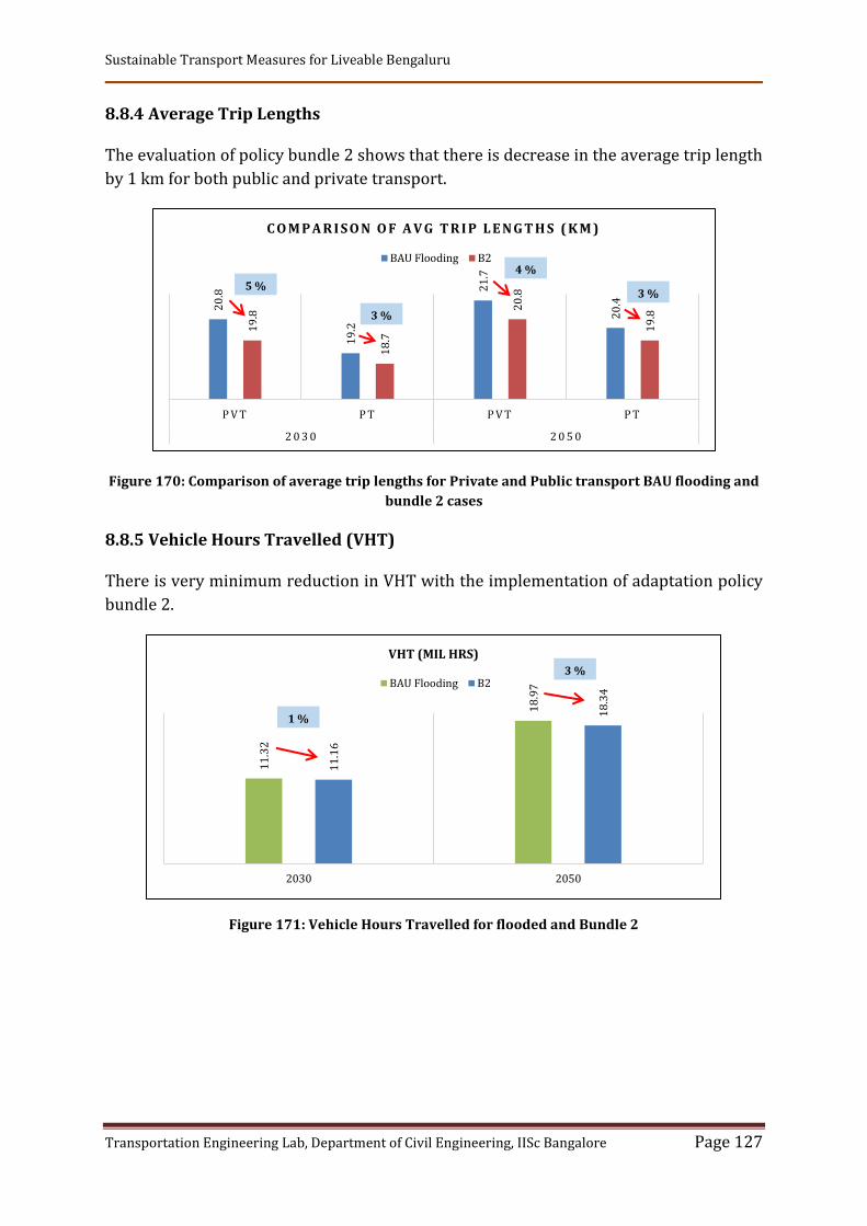
Sustainable Transport Measures for Liveable Bengaluru
Transportation Engineering Lab, Department of Civil Engineering, IISc Bangalore Page 127
8.8.4 Average Trip Lengths
The evaluation of policy bundle 2 shows that there is decrease in the average trip length
by 1 km for both public and private transport.
Figure 170: Comparison of average trip lengths for Private and Public transport BAU flooding and
bundle 2 cases
8.8.5 Vehicle Hours Travelled (VHT)
There is very minimum reduction in VHT with the implementation of adaptation policy
bundle 2.
Figure 171: Vehicle Hours Travelled for flooded and Bundle 2
20
.8
19
.2
21
.7
20
.4
19
.8
18
.7
20
.8
19
.8
P V T P T P V T P T
2 0 3 0 2 0 5 0
C O M P A R I S O N O F A V G T R I P L E N G T H S ( K M )
BAU Flooding B2
5 %
3 %
4 %
3 %
11
.32
18
.97
11
.16
18
.34
2030 2050
VHT (MIL HRS)
BAU Flooding B2
1 %
3 %

Sustainable Transport Measures for Liveable Bengaluru
Transportation Engineering Lab, Department of Civil Engineering, IISc Bangalore Page 128
8.9 ADAPTATION POLICY BUNDLE 3 EVALUATION RESULTS
Table 54: Policy Bundle 3
BUNDLE 3
Replacement of impermeable surfaces with permeable material in vulnerable areas
Providing proper drainage facilities at vulnerable areas
Rerouting people during flooding
8.9.1 Vehicle Kilometres travelled
Figure 172: Comparison of BAU Flooding VKT and Bundle 3
8.9.2 Cancelled Trips
The number of cancelled trips has been reduced from 2.8% in BAU scenario to 1.3% with
the implementation of bundle 3.
Table 55: Comparison of cancelled trips for BAU flood case and Bundle 3
Cancelled Trips
Flooding % Trips Cancelled B 3 % Trips Cancelled
160786 2.8 80393 1.3
8.9.3 Average Travel Speeds
The evaluation of bundle 2 shows that the average travel speed increases to 20.2kmph
and 17.6kmph for the years 2030 and 2050 with the implementation of these policies.
Since, this policy involves providing proper drainage facilities and also improving the
pavement surface there is considerable increase in the average vehicle speed.
41
.2
9.6
50
.8 57
.2
18
.1
75
.3
39
.8
9.3
4
49
.14
56
.4
17
.3
73
.7
P V T P T T O T A L P V T P T T O T A L
2 0 3 0 2 0 5 0
C O M P A R I S O N O F B A U F L O O D I N G V K T A N D B U N D L E 3
BAU- Flooding Bundle 3
3 %
3 %
3 % 1 %
4 %
2 %

Sustainable Transport Measures for Liveable Bengaluru
Transportation Engineering Lab, Department of Civil Engineering, IISc Bangalore Page 129
Figure 173: Comparison of travel speeds for BAU flooding and Bundle 3 cases
8.9.4 Average Trip Lengths
Figure 174: Comparison of average trip lengths for Private and Public transport BAU flooding and
bundle 3 cases
8.9.5 Vehicle Hours Travelled
Figure 175: Vehicle Hours Travelled for flooded and Bundle 3
16
.8
13
.2
20
.2
17
.6
2030 2050
AVERAGE SPEEDS (KMPH)
BAU Flooding B320 %
33 %
20
.8
19
.2 21
.7
20
.4
19
.34
17
.9 20
.2
19
.4
P V T P T P V T P T
2 0 3 0 2 0 5 0
C O M P A R I S O N O F A V G T R I P L E N G T H S ( K M )
BAU Flooding B37 %
7 %
7 % 5 %
11
.32
18
.97
10
.67
17
.8
2030 2050
VHT (MIL HRS)
BAU Flooding B3
6 %
6 %

Sustainable Transport Measures for Liveable Bengaluru
Transportation Engineering Lab, Department of Civil Engineering, IISc Bangalore Page 130
8.10 COMPARISON OF ADAPTATION POLICY BUNDLES RESULTS
8.10.1 Comparisons of VKT
Figure 176: Comparison of VKT’s between all scenarios for 2030
Figure 177: Comparison of VKT’s between all scenarios for 2050
Bundle 1 gives the best result comparing to other policy bundles. There is 4% and 3%
reduction in the vehicle kilometers travelled for the years 2030 and 2050 when
comparing with the BAU flooding condition.
48
50
.8
48
.6
49
.6
49
.14
B A U N O F L O O D B A U - F L O O D I N G B 1 B 2 B 3
VK
T (
MIL
KM
)
SCENARIOS
V K T 2 0 3 0 ( M I L K M S )
4 %
72
.1
75
.3
73
.1
74
.4
73
.7
B A U N O F L O O D I N G
B A U - F L O O D I N G B 1 B 2 B 3
VK
T (
MIL
KM
S)
SCENARIOS
V K T 2 0 5 0 ( M I L K M S )
3 %

Sustainable Transport Measures for Liveable Bengaluru
Transportation Engineering Lab, Department of Civil Engineering, IISc Bangalore Page 131
8.10.2 Comparison of Vehicle travel speeds
Figure 178: Comparison of Avg. travel speed of all scenarios for 2030
Figure 179: Comparison of Avg. travel speed of all scenarios for 2050
The policies in bundle 1 include both land use and infrastructure development and hence
the average vehicle speed has been increased by 21% and 45% for the years 2030 and
2050 when comparing with the BAU flooding condition.
25
.4
16
.8
21
.3
18
.7 20
.2
B A U - N O F L O O D I N G
B A U -F L O O D I N G
B 1 B 2 B 3
AV
G T
RA
VE
L S
PE
ED
(K
MP
H)
SCENARIO
A V G . T R A V E L S P E E D S ( K M P H ) - 2 0 3 0
21 %
23
.6
13
.2
19
.1
14
.3
17
.6
B A U - N O F L O O D I N G
B A U -F L O O D I N G
B 1 B 2 B 3
AV
G T
RA
VE
L S
PE
ED
(K
MP
H)
SCENARIO
A V G . T R A V E L S P E E D S ( K M P H ) - 2 0 5 0
45%

Sustainable Transport Measures for Liveable Bengaluru
Transportation Engineering Lab, Department of Civil Engineering, IISc Bangalore Page 132
8.10.3 Comparison of average trip lengths
Figure 180: Comparison of Avg trip length of PVT vehicles for 2030
Figure 181: Comparison of Avg trip length of PVT vehicles for 2050
18
.17
21
.7
19
.1
20
.8
20
.2
B A U - N O F L O O D I N G
B A U -F L O O D I N G
B 1 B 2 B 3
TR
IP L
EN
GT
H (
KM
)
SCENARIO
A V G T R I P L E N G T H ( K M ) - P R I V A T E V E H I C L E S - 2 0 5 0
12 %
17
.4
20
.8
18
19
.8
19
.34
B A U - N O F L O O D I N G
B A U -F L O O D I N G
B 1 B 2 B 3
TR
IP L
EN
GT
H (
KM
)
SCENARIO
A V G . T R I P L E N G T H ( K M ) - P R I V A T E V E H I C L E S - 2 0 3 0
13 %
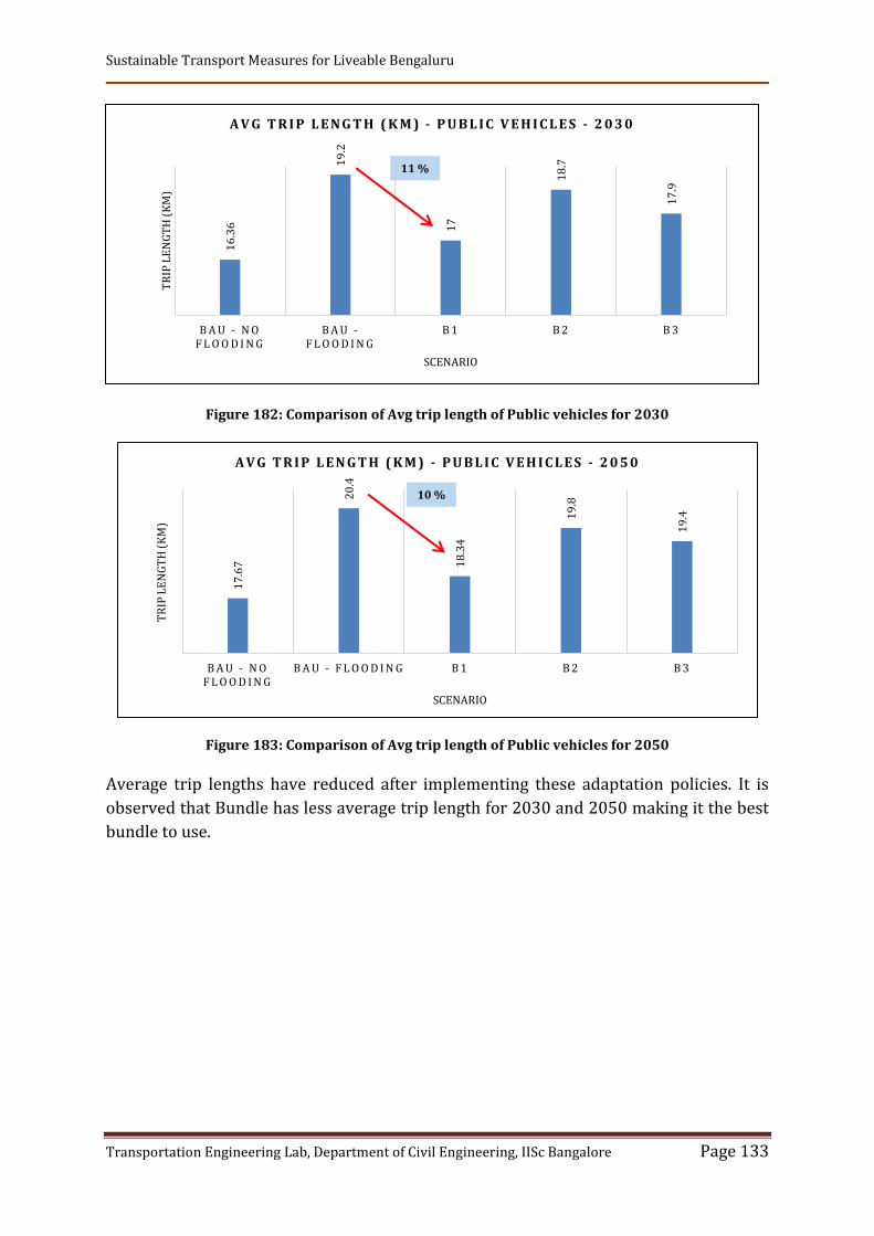
Sustainable Transport Measures for Liveable Bengaluru
Transportation Engineering Lab, Department of Civil Engineering, IISc Bangalore Page 133
Figure 182: Comparison of Avg trip length of Public vehicles for 2030
Figure 183: Comparison of Avg trip length of Public vehicles for 2050
Average trip lengths have reduced after implementing these adaptation policies. It is
observed that Bundle has less average trip length for 2030 and 2050 making it the best
bundle to use.
17
.67
20
.4
18
.34
19
.8
19
.4B A U - N O
F L O O D I N GB A U - F L O O D I N G B 1 B 2 B 3
TR
IP L
EN
GT
H (
KM
)
SCENARIO
A V G T R I P L E N G T H ( K M ) - P U B L I C V E H I C L E S - 2 0 5 0
10 %
16
.36
19
.2
17
18
.7
17
.9
B A U - N O F L O O D I N G
B A U -F L O O D I N G
B 1 B 2 B 3
TR
IP L
EN
GT
H (
KM
)
SCENARIO
A V G T R I P L E N G T H ( K M ) - P U B L I C V E H I C L E S - 2 0 3 0
11 %

Sustainable Transport Measures for Liveable Bengaluru
Transportation Engineering Lab, Department of Civil Engineering, IISc Bangalore Page 134
8.10.4 Comparison of Vehicle Hours Travelled
Figure 184: Comparison of VHT for BAU flood and BAU No flood scenarios and Policy Bundles for
2030 & 2050
There is 9% and 8% reduction in vehicle hours travelled with the implementation of
policy bundle 1 compared to bundle 2 & 3 for the years 2030 & 2050 respectively.
8.10.5 Comparison of Cancelled Trips
Figure 185: Comparison of cancelled Trips for Adaptation Bundles
The evaluation of policy bundles shows that with the implementation of policy bundle 1
the cancelled trips can be zero which means that no trips will get cancelled with these
policies.
16
07
86
0
14
47
07
80
39
3
Flood B 1 B 2 B 3
Ca
nce
lle
d T
rip
s
Scenario
CANCELLED TRIPS
9.5
4 11
.32
10
.25
11
.16
10
.67
16
.61 18
.97
17
.38
18
.34
17
.80
B A U N O F L O O D I N G
B A U F L O O D I N G B 1 B 2 B 3
VH
T (
MIL
HR
S)
SCENARIO
V H T ( M I L H R S ) 2030 2050
8 %
9 %

Sustainable Transport Measures for Liveable Bengaluru
Transportation Engineering Lab, Department of Civil Engineering, IISc Bangalore Page 135
8.11 RESULTS AND DISCUSSIONS
In this chapter, adaptation modelling for urban transport identified locations that are
vulnerable to flooding are identified using flood maps.
It is clearly observed that the vehicle take longer paths than usual and some trips
even get cancelled due to this. To address these issues 3 policy bundles have been
formulated and evaluated for the flooding scenarios.
It is observed from the results, that the policy bundle 1 is giving best results
compared to bundle 2 and 3.
By implementing bundle 1 it is seen that the average trip length of the vehicles
reduced compared to BAU flooding scenario.
Likewise total vehicle kilometres travelled and cancelled trips are less bundle 1
scenario compared to bundle 2 & 3.
Zero cancelled trips are achieved with the implementation of bundle 1.

Sustainable Transport Measures for Liveable Bengaluru
Transportation Engineering Lab, Department of Civil Engineering, IISc Bangalore Page 136
9 CONCLUSION
This report contains the mitigation and adaptation measures that are
quantitatively evaluated thereby improving the liveability of Bengaluru in terms
of; reduced traffic congestion (VKT), reduced exhaust emissions (PM, CO, NOX, HC),
reduced greenhouse gas emissions (CO2), reduced carbon emission intensity,
increased consumer surplus of sustainable modes and also improved resiliency of
transportation system.
All the policies lead to a significant reduction in the total VKTs travelled when
compared to the business as usual scenario.
Total emissions from bus are higher compared to other modes. But when
emissions are estimated in terms of per capita (per passenger km), they are
considerably low.
Bundle 3 (Bundle 4) which is a comprehensive mixture of 7 policies gives the best
results with respect to VKT reduction, Improved Public Transport Share and
reduction in emissions.
The significant reduction in emissions is observed with the implementation of
bundle 4-scenario 4 which includes the electrification of all buses and cars.
Bundle 4 is a mixture of planning, regulatory, economic and technology
instruments.
The bundle 4 is evaluated with respect to four scenarios out of which the scenario
4 with the assumption that electricity will be produced 100% from the renewable
sources shows substantial reduction in emissions.
Thus, it is concluded and recommended that the implementation of bundle 4 along
with scenario 4 will result in considerable reduction in emissions from transport
sector. Although CO2 emission factor values are zero in scenario 4 it is suggested
that shifting towards mass transportation systems like Bus & Metro not only
reduces the emissions but also reduces the congestion on the roads by a great
amount.
A proper amalgamation of planning, regulatory, economic and technology
instruments incorporating the complete clean energy can help in improving the
sustainability of transportation systems thereby enhancing liveability of the city.
The bundle 4 – scenario 4 is implemented the total emission intensity will reduce
by 91% for the year 2030 and 96% for 2050.
The bundle 4 – scenario 4 is implemented the per-capita emission intensity will
reduce by 94% for the year 2030 and 99% for 2050, highlighting that
electrification of vehicles is the best solution with 100% electricity generation
from renewable sources.

Sustainable Transport Measures for Liveable Bengaluru
Transportation Engineering Lab, Department of Civil Engineering, IISc Bangalore Page 137
Urbanization has led to reduction in the pervious area thus leading to urban
flooding. Proper drainage facilities and using permeable roads at vulnerable
locations can reduce the surface runoff on the roads and helps in a better
movement of traffic.
In adaptation policy bundles, it is observed that implementation of policy bundle
1 is more effective compared to bundle 2 & 3. It is suggested a proper mixture of
land use and infrastructure related policies can help the city come out of the urban
flooding muddle.
Due to heavy flooding at certain locations it is observed that the trips from those
zones are cancelled. One interesting thing observed in this study is that the
implementation of Adaptation Bundle 1 resulted in zero cancelled trips. This
clearly states that with a proper management of land use and infrastructure
policies we can nullify the trips that get cancelled due to flooding and people can
still make trips in such extreme events.

Sustainable Transport Measures for Liveable Bengaluru
Transportation Engineering Lab, Department of Civil Engineering, IISc Bangalore Page 138
REFERENCES
1. Chandel M., “Estimation of Emission Factors for Different Vehicles” Centre for
Environmental Science and Engineering, Indian Institute of Technology Bombay,
2018.
2. CSTEP (2015). Need for Government Support for Public Bus Transport (CSTEP-
Report-2015-05)
3. Directorate of Census Operations Karnataka, "District Census Handbook Bangalore"
2011.
4. Directorate of Economics and Statistics, Bangalore,"State and District Domestic
Product of Karnataka", 2014 - 15.
5. Groupe SCE India Pvt. Ltd., "Bangalore Metropolitan Region Revised Structure Plan -
2031"
6. Pregnolato M, Ford A, Glenis V, Wilkinson S., and Dawson R., "Impact of Climate
Change on Disruption to Urban Transport Networks from Pluvial Flooding" Journal
of Infrastructure Systems, 23(4), 2017.
7. Rahul T. M., and Verma A., “A study of acceptable trip distances using walking and
cycling in Bangalore”, Journal of Transport Geography, vol. 38, pp. 106 - 113, 2014.
8. Ramachandra. T.V., Bharath Setturu and Bharath H. Aithal., 2012. "Peri-Urban to
Urban Landscape Patterns Elucidation through Spatial Metrics", International Journal
of Engineering Research and Development. Volume 2, Issue 12 (August 2012), pp. 58-
81.
9. Transport Department, Government of Karnataka, "Annual Report", 2015 - 16.
10. Verma, Rahul T. M., and Dixit M., “Sustainability impact assessment of transportation
policies – A case study for Bangalore city”, Case Studies on Transport Policy, vol. 3,
pp. 321 - 330, 2015.
11. Wilbur Smith Associates, "Comprehensive Traffic and Transportation Study for
Bangalore Metropolitan Region (CTTS)”, June 2010.
12. https://scroll.in/article/847397/how-bangalore-went-from-being-indias-most-
liveable-city-to-a-dystopia-in-the-making
13. http://ces.iisc.ernet.in/energy/wetlands/sarea.html
14. https://www.mybmtc.com/en/bmtc_glance
15. http://english.bmrc.co.in/News/NewsSection

Which role shall the different transport modes play?
Push-and-Pull concept:Which modes need support, which modes need restrictions?
Push: parking management, access restrictions, etc.
Pull: dense bus network, high quality bus services, etc.
Push and Pull: separate bus lanes, priority for buses at traffic signals, etc.
Transportation Engineering Lab,Department of Civil Engineering,
Indian Institute of Science (IISc), Bangalore