Individual values of X
65
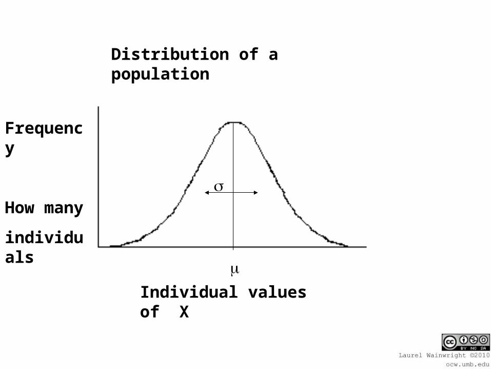
Individual values of X Frequenc y How many individu als Distribution of a population
-
Upload
eliana-richmond -
Category
Documents
-
view
15 -
download
0
description
Distribution of a population. Frequency How many individuals. . . Individual values of X. Distribution of a sample. Frequency How many individuals. s. Individual values of X. - PowerPoint PPT Presentation
Transcript of Individual values of X
Individual values of X
Frequency
How many
individuals
Distribution of a population

Individual values of X
Frequency
How many
individuals
s
Distribution of a sample
X

Distribution of a sample: The way in which the individual scores within a sample are spread out in relation to the mean.
Sampling Distribution: The way in which sample means, drawn from the same population, spread out from the population mean.

Sampling Distribution
Mean values of all possible samples.
Frequency
How many
samples
x
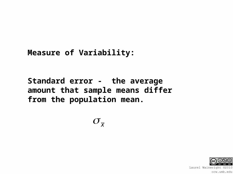
Measure of Variability:
Standard error - the average amount that sample means differ from the population mean.
x
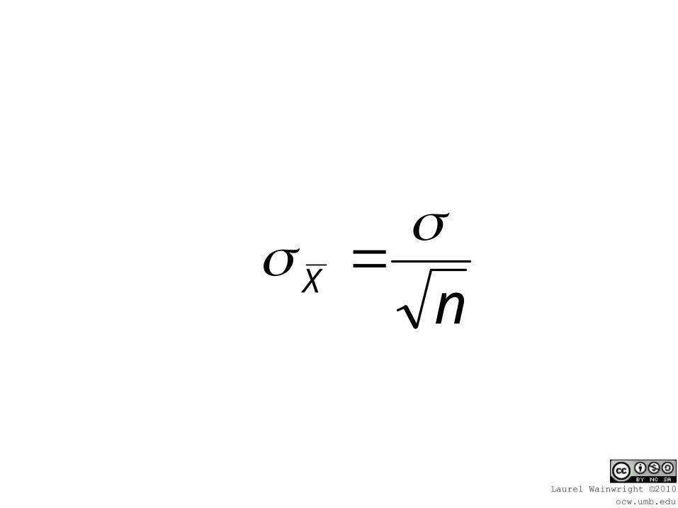
nX

If:
a) randomly select enough samples
b) all samples were the same size

Then:
The distribution of those sample means would form a normal distribution.

We can use the normal distribution to predict the likelihood of randomly selecting samples with particular means.

X
XZ
nX

= 45 = 10 N = 16
What is the likelihood that a sample, selected at random from this population, would have a mean of 43 or less?
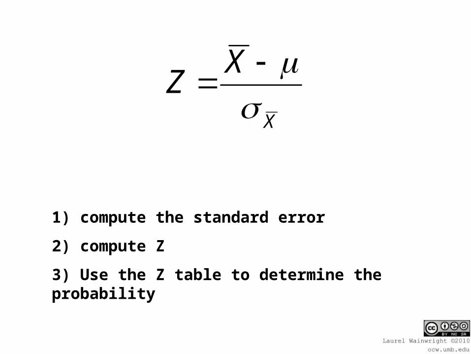
1) compute the standard error
2) compute Z
3) Use the Z table to determine the probability
X
XZ

= 45 = 10 N = 16
1) compute the standard error
nX
43X

= 2.5x
16
10x
4
10x

2) compute Z using the standard error
x
z5.2
4543 z
Z = - .8

Reminders about Z table:
a column: Z score
b column: prob. between mean and Z
c column: prob. beyond z into the tail
b column + c column = .5000

b cbc

Z table:
z score
a b c
.79 .2852 .2148
.80 .2881 .2119
.81 .2910 .2090

Z table:
z score
a b c
.79 .2852 .2148
.80 .2881 .2119
.81 .2910 .2090

The prob. that a sample mean would below 43 is .2119.

Raw means 43 45
Z scores - .8 0
.2881 or 28.81%
.2119 or
21.19%
.5000 or 50.0 %
With the probability info we can:
- Determine how often we expect a
particular sample to be drawn.
- Establish the probability that a
particular sample that we have
is a random sample.
You develop an expensive training program for athletes.
You say that your program reduce event times for runners.
Typical running time: 50 sec.
After your program the group’s average running time is 49 sec.
Is the program effective,
or is this random variability?
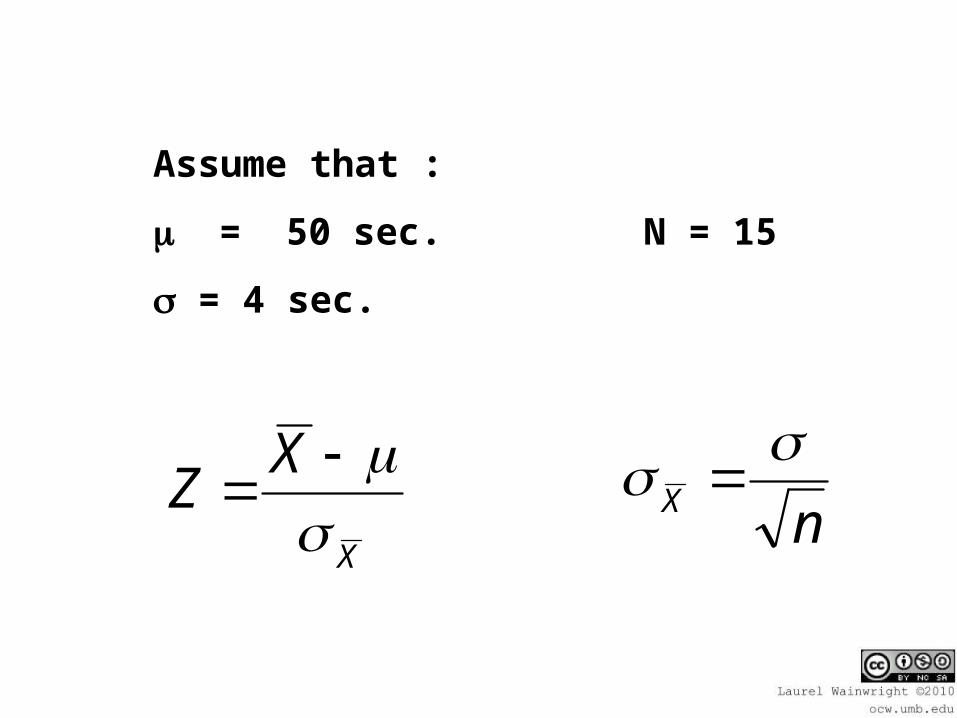
Assume that :
= 50 sec. N = 15
= 4 sec.
nX
X
XZ

standard error = 1.03
87.3
4
87.315
15
4
X
X

Z = - .97
03.1
1z
03.1
5049 z

Probability that a sample would have a mean of 49 or a more extreme score?
P = .1660

- .97 0
49 50
33.40%
16.60%
Raw score
Z score
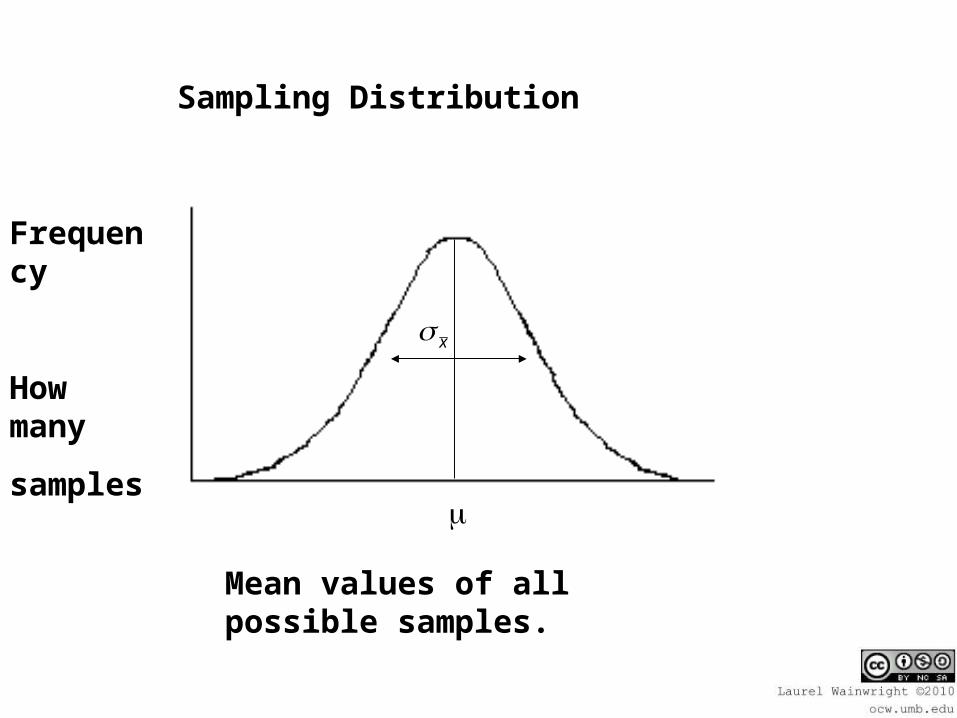
Sampling Distribution
Mean values of all possible samples.
Frequency
How many
samples
x

The convention is that we will assume that a sample is different from the population mean for reasons other than chance when the probability of randomly selecting the sample is less than or equal to .05 (5%)

Statistical Significance:
The outcome could occur by chance alone less than 5% of the time.

Null hypothesis: Mathematical statement that describes the population in the absence of any treatment.
Ho : = 50
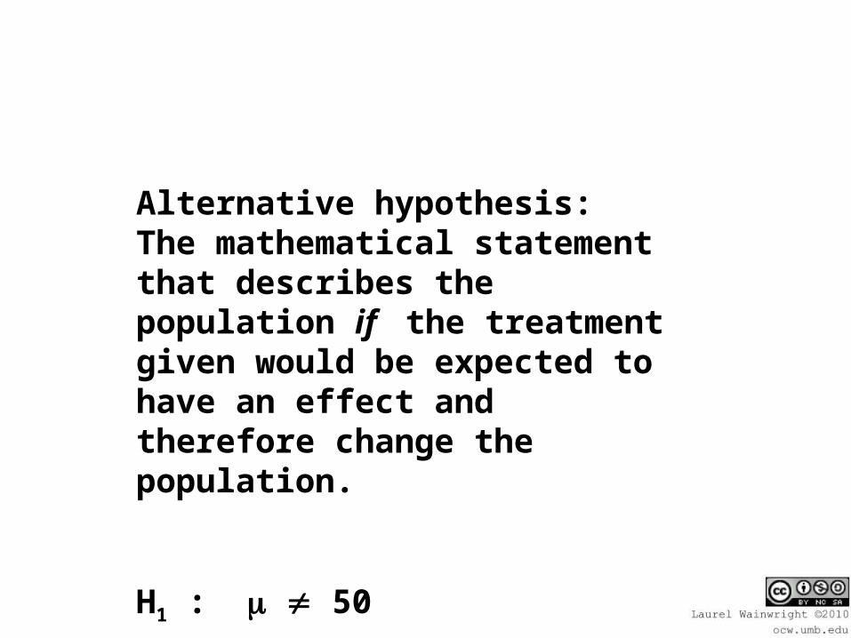
Alternative hypothesis: The mathematical statement that describes the population if the treatment given would be expected to have an effect and therefore change the population.
H1 : 50

If an outcome is statistically significant we reject the null hypothesis and accept the alternative.
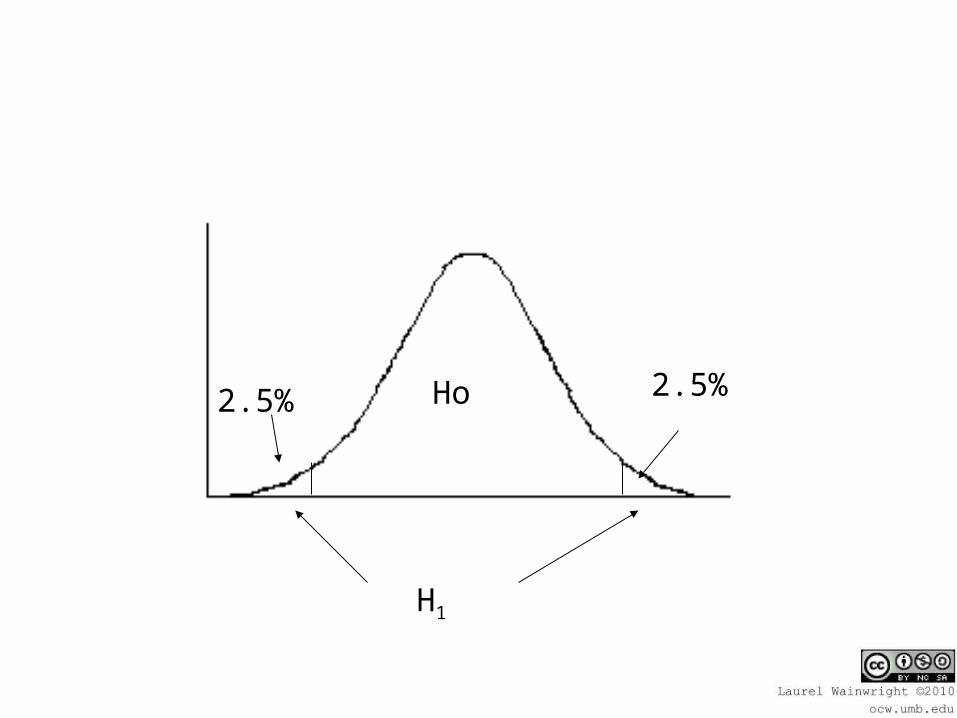
2.5% 2.5%Ho
H1

Why is the 5% split into two parts?
H1 : 50
This doesn’t suggest the direction of an unusual outcome.
Samples means much less than the population mean of 50 as well as samples means much greater than 50 would be unusual.

50
Ho : = 50
H1 : 50
2.5%
2.5%
This is know as a two tailed test.
Both tails of the distribution are included as possible outcomes in the hypothesis statement.
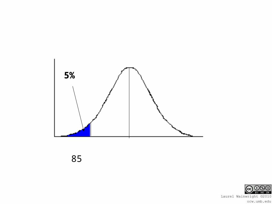
Assume a teacher knows that students generally have an average score on a test of 85. The standard deviation of all of the students has been 7 points.
Ho : = 85
H1 : 85
The teacher uses a new curriculum this year and finds that the class (N = 20) has an average on the test of 81.
Has this curriculum made a difference in the performance of the class?
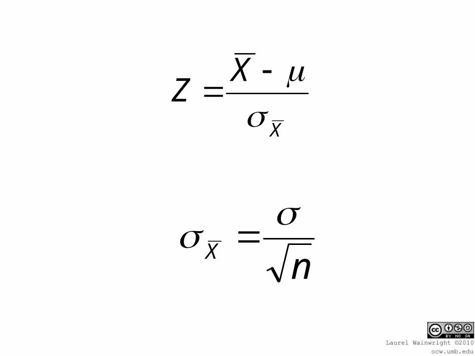
X
XZ
nX
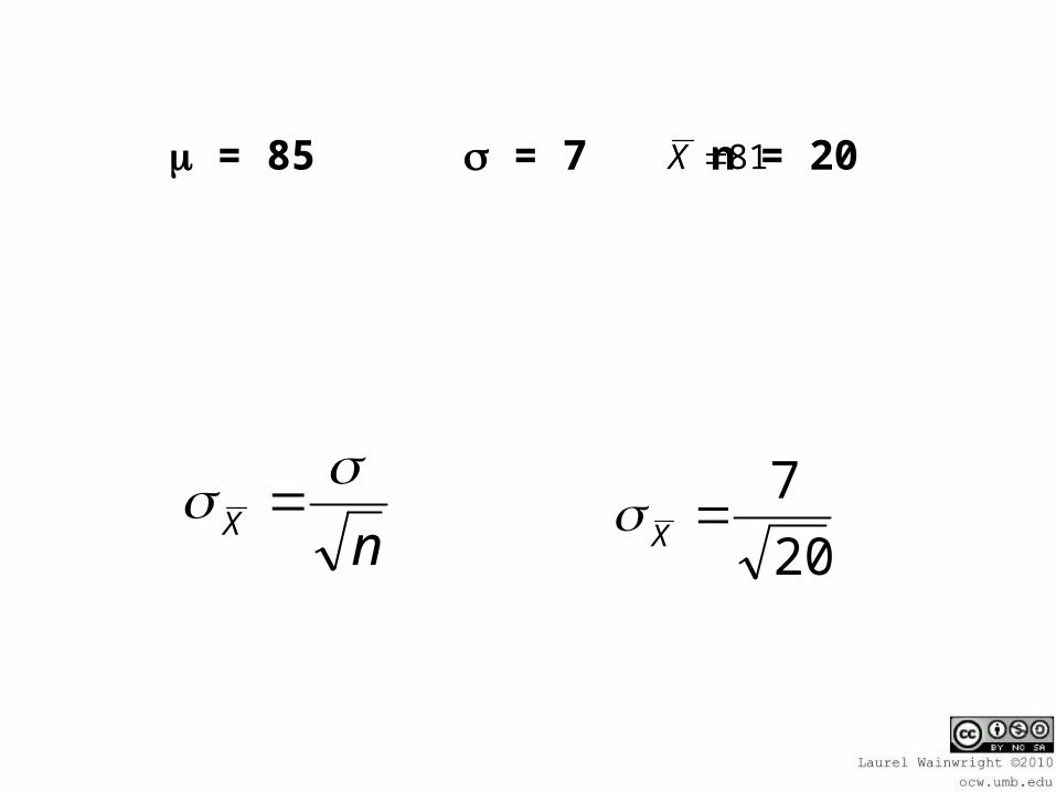
= 85 = 7 n = 20
nX
20
7X
81X
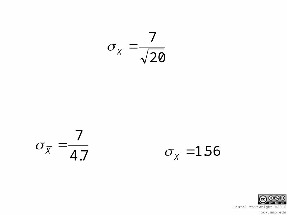
20
7X
7.4
7X 56.1X

81 - 85
Z =
1.56
Z = --2.56

From the Z table:
Prob. of a Z score between 0 and
2.56 is .4948 (col. B)
The prob. of a Z score beyond 2.56 is .0052 (col. C)

.0052 < .05
Therefore this qualifies as a statistically significant event.

Sample means 81 85
Z scores -2.56 0
H1H1

Conclusion:
Reject the null hypothesis.
This curriculum probably caused the class to perform differently than the population as a whole.

Could our conclusion be wrong?
It is possible (although unlikely) that a sample that had a mean of as low as 81 could have been selected at random from the population.
In other words, it is possible (although unlikely) that the curriculum had no effect on the sample.

Type One Error (alpha error, )
When you reject the null and it is actually true.
Type two error (beta error, )
Accept the null hypothesis (saying that the independent variable has no effect) when the null is false.

Ho : = 85
H1 : 85
One tailed test:
When the alternative hypothesis predicts a direction.
H1 : < 85
85
5%

Z score where 2.5% of the distribution lies in the tail:
Z = + 1.96
Critical value for a two tailed test.
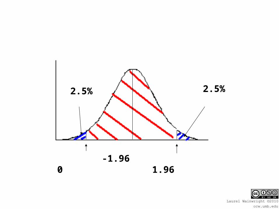
-1.96 0 1.96
2.5%2.5%

Z score where 5% of the distribution lies in the tail:
Z = + 1.65
Critical value for a one tailed test.
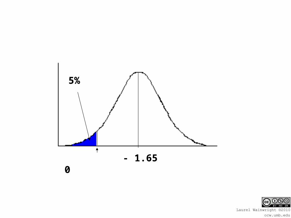
- 1.65 0
5%

0 1.65
5%


![Intermediate Track III GL Case Study...Actual Values (slide 6) Transformed Values Fitted Values Cumulative Factors X Var. Y Variable X' Y' X Y X Y Age LDF's X ln[ln(Y)] Age LDF's Age](https://static.fdocuments.net/doc/165x107/60bf93c0f1310212c7751660/intermediate-track-iii-gl-case-study-actual-values-slide-6-transformed-values.jpg)