
Individual responses to BTS and the Forecasting of ... responses to BTS and the ... used are the...
43
OECD - EU Joint Workshop on Business and Consumer Surveys, Brussels, November, 14-15, 2005 Revised version, February 2006 Individual responses to BTS and the Forecasting of Manufactured Production: An assessment of the Mitchell, Smith and Weale dis-aggregate indicators on French Data by Olivier Biau, Hélène Erkel-Rousse and Nicolas Ferrari * (INSEE, France) * At the moment when the empirical study was performed (in Spring 2005), Olivier Biau and Nicolas Ferrari were both members of the Business Survey Unit of the French statistical institute INSEE ([email protected], [email protected]). Hélène Erkel-Rousse is the head of the Macroeconomic Studies Unit in INSEE ([email protected]). The empirical work was carried out in April 2005. We thank Fabien Toutlemonde for his discussion of a previous version of the paper at the DEEE Workshop, INSEE, Paris, June, 29, 2005, as well as the participants of the OECD-European Commission joint Workshop, Brussels, 15, 2005, for their questions and comments. We are also grateful to Philippe Scherrer, Dominique Ladiray and two anonymous referees for helpful comments. All remaining errors are ours. The views expressed here are those of the authors and do not necessarily represent those of INSEE.
Transcript of Individual responses to BTS and the Forecasting of ... responses to BTS and the ... used are the...

OECD - EU Joint Workshop on Business and Consumer Surveys, Brussels, November, 14-15, 2005 Revised version, February 2006
Individual responses to BTS and the Forecasting of Manufactured Production:
An assessment of the Mitchell, Smith and Weale dis-aggregate indicators on French Data
by Olivier Biau, Hélène Erkel-Rousse and Nicolas Ferrari*
(INSEE, France)
* At the moment when the empirical study was performed (in Spring 2005), Olivier Biau and Nicolas
Ferrari were both members of the Business Survey Unit of the French statistical institute INSEE ([email protected], [email protected]). Hélène Erkel-Rousse is the head of the Macroeconomic Studies Unit in INSEE ([email protected]). The empirical work was carried out in April 2005. We thank Fabien Toutlemonde for his discussion of a previous version of the paper at the DEEE Workshop, INSEE, Paris, June, 29, 2005, as well as the participants of the OECD-European Commission joint Workshop, Brussels, 15, 2005, for their questions and comments. We are also grateful to Philippe Scherrer, Dominique Ladiray and two anonymous referees for helpful comments. All remaining errors are ours. The views expressed here are those of the authors and do not necessarily represent those of INSEE.

OECD-EU Joint Workshop on Business and Consumer Tendency Surveys, Brussels, November, 14-15, 2005 - revised version
Abstract:
In this paper, we compare the performances of balances of opinion with those of competing dis-aggregate indicators derived from the Mitchell, Smith and Weale (MSW) methodology as concerns the one-quarter forecasting of the manufactured production growth rate. The data used are the Business Tendency Survey in Industry carried out by INSEE and the French Quarterly Accounts. The dis-aggregate indicators are derived from the entrepreneurs’ individual responses to the survey questions relating to either past or expected production. They are of two kinds: the parametric indicators are based on ordered discrete-choice models at the firm level (polytomic logit models); the other indicators are derived from simpler non-parametric methodology. MSW’s applications to British and German data suggest that their indicators perform better than a set of three competing aggregate indicators, but they do not obtain the same result on Portuguese and Swedish data. Based on a thorough out-of-sample analysis, our application to French data leads to the conclusion that the forecast performances of the MSW are less good or, at best, equivalent to those of the balances of opinion, depending on the models used.
Keywords: Business Tendency Surveys, quantification, balance of opinion, indicators, short-term forecasting, manufactured production.
JEL Classification: C8, C42, C53, E23, E37, L60.
Résumé :
Dans cette étude, nous comparons les performances de soldes d’opinion et d’indicateurs concurrents proposés par Mitchell, Smith et Weale (MSW) pour la prévision à un trimestre du taux de croissance de la production manufacturière. Les sources utilisées, françaises, sont l’enquête sur la situation et les perspectives dans l’industrie et les comptes trimestriels publiés par l’INSEE. Les indicateurs de MSW sont élaborés à partir de l’agrégation de prévisions du taux de croissance de la production manufacturière (globale ou par secteurs) effectuées au niveau de chaque entreprise sur la base de leurs réponses individuelles à la question sur la production passée ou prévue. Deux types d’indicateurs sont construits : les premiers, de type paramétrique, sont fondés sur des modèles à choix discrets ordonnés au niveau des réponses individuelles (modèles logit polytomiques). Les seconds, de type non paramétrique, sont construits de manière plus simple. Les applications de MSW à des données britanniques et allemandes établissent que leurs indicateurs sont plus performants que plusieurs indicateurs agrégés classiques, mais ils n’obtiennent pas le même résultat sur données portugaises et suédoises. Notre application sur données françaises, fondée sur une analyse hors échantillon détaillée, aboutit à la conclusion que les performances prédictives des indicateurs de MSW s’avèrent inférieures ou, au mieux, équivalentes à celles des soldes d’opinion, selon les modèles utilisés.
Mots clef : enquêtes de conjoncture, quantification, solde d’opinion, indicateur, prévision conjoncturelle, production manufacturière.
2

Individual responses to BTS and the Forecasting of Manufactured Production...
1. Introduction
Due to their early release (by the end of the month of their realization), business tendency survey (BTS) results are used widely to provide indicators of economic activity ahead of the publication of data from quarterly national accounts. In particular, BTS data allow one to elaborate short-term forecasting models of the main aggregates of the national accounts on the basis of summary indicators derived from the surveyed's responses.
Most BTS questions are qualitative and require either a positive response (« up » or « superior to average »), or an intermediate one (« stable » or « close to average ») or, else, a negative one (« down » or « inferior to average »). A large majority of summary indicators derived from the individual responses to these questions result from standard quantification methods, most of them being based on a combination of the percents of positive, stable and negative responses. For instance, the balance of opinion, which is the most currently used indicator for short-term analysis, is defined as the difference between the (generally weighted) proportion of respondents who report the positive response and that of respondents who report the negative one. These kinds of indicators are referred to as “aggregate indicators” as they are derived from aggregate pieces of information on the surveyed’s responses.
As such, aggregate indicators encounter some criticism, due to the fact that they do not exploit the heterogeneity in the surveyed’ individual responses. In this respect, Mitchell, Smith and Weale (MSW) (2002, 2004, 2005) present alternative kinds of dis-aggregate indicators1 of economic activity relating firms' categorical responses to official data using ordered discrete-choice models. Their applications to firm-level survey data from the Confederation of British Industry and from the German institute IFO suggest that these alternative indicators of manufacturing output growth provide more accurate early estimates of manufacturing output growth than a set of classical aggregate indicators (from which the balance of opinion is excluded). Conversely, their applications to Portuguese and Swedish survey data conclude in favor of the aggregate indicators.
The object of the present paper is to compare the short-term forecast performances of four kinds of dis-aggregate indicators based on the MSW (2002, 2004) methodology to those of the balances of opinion. In this purpose, we apply the MSW (2002, 2004) methodology to the quarterly responses given to two questions asked in the BTS in industry carried out by the French institute INSEE, namely those relating to past and expected production. We, then, compare the one-horizon forecast performances of the dis-aggregate indicators derived from MSW (2002, 2004) to those of the corresponding balances of opinion as concerns the short-term forecasting of the manufacturing production quarterly growth rate. Note that, in practice, these two balances of opinion prove to be homothetic to the corresponding “Pesaran”
1 These are dis-aggregate indicators in the sense that their elaboration methods exploit the
heterogeneity in the surveyed’s responses.
3

OECD-EU Joint Workshop on Business and Consumer Tendency Surveys, Brussels, November, 14-15, 2005 - revised version
indicators2 used by MSW (2002, 2004), which enables us to compare our results to theirs.
A thorough out-of-sample analysis enables us to conclude in the case of the French application that the balances of opinion lead to better or, at least, as accurate short-term forecasts of the manufacturing production growth rate than the MSW dis-aggregate indicators, depending on the model used. These findings are consistent with those obtained by MSW (2004-2) on Portuguese and Swedish data, but not on British and German data. In the case of the French application, the comparative advantages of the MSW indicators do not seem to be clear with respect to the balances of opinion, which are simpler to implement and subject to lower revisions (if any) across time.
The second section of the paper briefly reminds the reader with the most current aggregation and quantification methods leading to short-term indicators derived from BTS survey results. The third section details the MSW methodology and indicators, and summarizes the main results they obtain in their successive papers and reports (2002, 2004, 2005). The fourth section presents the French data and our methodology. The fifth section describes and comments our main results. Finally, the sixth section concludes and suggests some possible tracks for future research.
2. Aggregation and quantification of BTS responses:
Main approaches
A large majority of summary indicators derived from the individual responses to qualitative BTS questions (among which most are three-modality questions) result from standard aggregation and quantification methods. The percents of positive, stable and negative responses to the questions, although they constitute the exhaustive statistics of the individual responses, are not often used as such. This stems from the fact that sets of three series are neither easy to follow over time nor synthetic enough indicators. That is why univariate indicators are preferred in general. Consequently, most aggregate indicators relating to a specific three-modality question are based on various combinations of these three percents.
This is the case for the indicator most currently used in short-term analysis, namely the balance of opinion. The latter aggregate indicator is, in fact, defined as the difference between the (generally weighted) proportion of respondents who report a positive response and that of respondents who report a negative one. Balances of opinion are interesting indicators in many respects. They are easy to implement. As univariate series, they are simple to read and follow over time, to the expense of a, generally, acceptable loss of information with respect to the corresponding exhaustive three-dimension statistics. Besides, balances of opinion are subject to limited revisions across time, if not to no revision at all, depending on the survey producers’ methodology. Furthermore, the main balances of opinion (notably those relating to activity) are highly correlated with the corresponding 2 The “Pesaran” indicator is derived from the “regression” approach - cf. section 2 and sub-section 6.1.
4

Individual responses to BTS and the Forecasting of Manufactured Production...
aggregates of interest, even though they are generally smoother (and therefore easier to read). This is the case, for instance, for the balances of opinion relating to past and expected manufactured production derived from the BTS in industry carried out by the French statistical institute INSEE, hereafter referred to as the INSEE Industry survey (see Fig. 1 below). All these interesting properties explain why the balances of opinion are the main (if not the quasi-exclusive) kinds of indicators used by short-term analysts. Note that Theil (1952) and subsequent Fansten (1976) suggest some theoretical foundations for the balances of opinion, even though the latter foundations appear to be valid under fairly restrictive assumptions. All in all, due to their good empirical properties, the balances of opinion prove to be very useful, being well adapted to the quick production and release conditions of BTS in the optic of synthetic communication and generalist use in short-term analysis. However, this does not prevent one from trying to elaborate in parallel optimized indicators with respect to a specific objective3.
Figure 1: Balances of opinion relating to manufactured production and the manufacturing production quarterly growth rate
-40
-30
-20
-10
0
10
20
30
40
1990 1991 1992 1993 1994 1995 1996 1997 1998 1999 2000 2001 2002 2003 2004-3
-2
-1
0
1
2
3
4
<- Balance on past production <- Balance on expected productionmanufacturing production growth rate ->
Sources : INSEE Industry survey and French Quarterly Accounts (situation in Spring 2005, when the empirical
study was performed). The balance relating to past production is shifted by one quarter with respect to the two other series so that the reference periods of all series be identical for every quarter t.
In this respect, the literature suggests miscellaneous aggregation methods aiming to
define the best possible combinations of individual responses to BTS in order to elaborate indicators reaching some specific objective such as: describing the current position in the cycle (coincident indicator), assessing the probability of an acceleration or a slowdown in the short run (turning-point indicator) or, else, enabling one to make early forecasts of a
3 For instance, Driver and Urga (2004) aim to find the best transformation of the quantitative survey
responses given to the British Industrial Trends survey carried out by the CBI (Confederation of British Industries), in the sense that this transformation enables them to obtain the best regression results of actual data relating to a macroeconomic aggregate of interest on the transformed qualitative series. This specific aim refers to the discussion below on leading indicators.
5

OECD-EU Joint Workshop on Business and Consumer Tendency Surveys, Brussels, November, 14-15, 2005 - revised version
macroeconomic aggregate (leading indicator)4. The majority of indicators of that kind, however, remain aggregate indicators. Balances of opinion or combinations of carefully selected sets of balances, or else more complex derivations from balances (as concern turning-point indicators, especially) are often privileged by short-term analysts.
As far as coincident indicators are concerned, the economic sentiment indicator published by the European Commission (DG-ECFIN), for instance, is defined as the weighted means of five components (the confidence indicators), calculated by summation of a certain number of normalized balances of opinion previously selected for their strong link with some macroeconomic or sector aggregates - cf. European Commission (2004). Applying the OECD methodology, the Italian institute ISAE publishes a confidence indicator in industry derived from the means of three transformed balances (the judgment on orders, the tendency of production and the level of supplies). Similarly, the IFO business climate index for Germany is defined as the means of the transformed balances relating to the current business situation and the entrepreneurs’ expectations for the next six months derived from the IFO business surveys in the industry and trade sectors5. The INSEE synthetic indicator in industry is also defined as a linear combination of several normalized balances of opinion, but, in this case, the weighting scheme of the balances is endogenously estimated, using factor analysis techniques6. The synthetic indicator for Euroland introduced by Lenglart and Toutlemonde (2002) and also published by INSEE results from the same methodology and combines a number of balances of opinion derived from the biggest EU Member States. The newly published INSEE synthetic indicator in services is, however, estimated using a more complex methodology, still based on dynamic factor analysis but allowing for the combination of a set of balances of heterogeneous periodicities and available on different periods (Cornec and Deperraz, 2005). Note that the introduction of indicators derived from BTS into factor models can be considered as a means to link BTS data to some latent economic variable reflecting the business cycle (in a given sector or at macroeconomic level, depending on the set of indicators used)7. The resulting synthetic indicator, or common factor, is, then, supposed to reflect this latent variable (also see below).
Many turning-point indicators are derived from the estimation of two-state hidden Markov processes, thus following Hamilton (1989, 1990) and subsequent Lahiri and Wang (1994). For instance, the monthly turning-point indicator published by INSEE is based on a two-step methodology suggested by Grégoir and Lenglart (2000), which consists in extracting the innovations contained in six balances of opinion from the INSEE Industry survey at a first
4 On leading indicators in general, see Lahiri and Moore (1991), for instance. 5 Source: IFO website (http://www.cesifo-group.de/). 6 Cf. Doz and Lenglart (1996-1999) for a detailed presentation. A quick definition (in French) can be
found on the INSEE website (http://www.insee.fr/fr/ indicateur/ indic_conj/donnees/doc_idconj_11.pdf). Also see Bouton and Erkel-Rousse (2002) for the elaboration of sectoral common factors (in industry, services, retail trade, construction, and wholesale trade) derived from the same methodology.
7 For methodological explanations or empirical applications of this kind of approach, see Stone (1947), Sargent and Sims (1977), Stock and Watson (2002), Doz and Lenglart (1996-1999), Forni, Hallin, Lippi and Reichlin (2001), Cornec and Deperraz (2005), among others.
6

Individual responses to BTS and the Forecasting of Manufactured Production...
stage, and then deriving the probabilities of an acceleration and a deceleration in the short run from the signs of these innovations using a hidden Markov model at a second stage. The turning-point indicator is, then, defined as the difference between the estimated probability of an acceleration and that of a deceleration. The European Commission and the Bank of Spain have developed a turning-point indicator based on a similar approach, but mixing BTS survey results (those encompassed in the European Commission’s industrial confidence indicator) with the industrial production index for the Euro zone; the turning-point indicator is defined as the estimated probability of a deceleration (Bengoechea and Pérez-Quirós, 2004).
As regards short-term forecasting, the most current approaches in the literature consist in combining the percents of positive and negative responses by linking them to the (observed or latent) macroeconomic aggregate of interest. This is the case for the two well-known approaches referred to as the “probability” approach and the “regression” approach8. Sketched by Theil (1952) and developed by Carlson and Parkin (1975), the “probability” approach is based on the assumption that the response of a given firm concerning the aggregate of interest such as output growth is derived from a subjective probability density function for this aggregate which may be firm-specific and is conditional to information available to the firm. The means of this subjective probability density is an unbiased predictor for the aggregate of interest: it can be derived from the percents of responses “up” and “down” to the question relating to the aggregate of interest under some technical conditions identifying the distribution functions of the latter percents9. More simply, the “regression” approach, introduced by Anderson (1952) and developed by Pesaran (1984), comes to regress the macroeconomic aggregate of interest on the (appropriately weighted) percents of positive and negative responses to the question relating to this aggregate10. Two other approaches also based on a combination of the percents of responses “up” and “down” can be mentioned too. The “latent factor” approach (D’Elia, 1991) regards the percentages of positive, neutral and negative answers as functions of a common “latent measure” of the aggregate of interest observed by the surveyed, but not by statisticians. Multivariate factor analysis techniques enable him to estimate the dynamics of the variations of this latent factor. In the “inverted regression” approach, introduced by Cunningham, Smith and Weale (1998), the categorical survey responses of each firm are determined by a firm-specific latent variable related to the macroeconomic aggregate of interest through a linear model, according to a rule which is common to all firms. Some links can be established between these different approaches and each of them can be proxied by balances of opinion under some conditions (Anderson, 1952; Theil, 1952; Lankes and Wolters, 1988; Mitchell, Smith and Weale, 2004; D’Elia, 2005). 8 Cf. Nardo (2003), Mitchell, Smith and Weale (2002, 2004) and D’Elia (2005) for more detailed
presentations. 9 For examples of papers applying the “probability” approach, see Carlson (1975), Wachtel (1977),
Fishe and Lahiri (1981), Batchelor (1981), Batchelor and Orr (1987), Dasgupta and Lahiri (1992), Lee (1994), Balcombe (1996), and Berk (1999), among others.
10 The “regression” approach is used, for example, by the Bank of England - see Britton, Cutler and Warlow (1999). There have been numerous extensions of the “probability” and “regression” approaches - see Pesaran (1984, 1987), Smith and McAleer (1995) or Driver and Urga (2004).
7
OECD-EU Joint Workshop on Business and Consumer Tendency Surveys, Brussels, November, 14-15, 2005 - revised version
Note that most indicators used for short-term forecasting in operational context are specific balances of opinion chosen for their advanced properties or composite indicators combining a set of selected balances. Nonetheless, the use of indicators based on percents of positive, stable and negative responses rather than on balances is also recommended by a minority of short-term analysts. In an application to French data, for instance, Hild (2002) suggests that the introduction of percents of responses of different kinds in calibration models might enable one to improve the short-term forecasting of some macroeconomic aggregates. Hild (2005), then, refines the approach based of percents of responses “up”, “stable” or “down” by suggesting the use of a synthetic indicator (estimated using dynamic factor analysis) derived from non-standard elementary indicators relating to a set of questions from the INSEE industry survey. The latter elementary indicators are based on percents of entrepreneurs who change their responses (for instance switching from “stable” to “up” or to “down”) from one survey to the next one. The underlying intuition is that these modifications in entrepreneurs’ responses may constitute an early sign of a change in the trend of activity.
Despite their intensive use and established usefulness, the aggregate indicators encounter some criticism, as they do not exploit the heterogeneity of the individual responses to BTS. Some authors suggest the use of alternative “dis-aggregate” indicators, whose principle consists precisely in exploiting such information. In particular, Mitchell, Smith and Weale (MSW) (2002, 2004, 2005) propose two indicators relating firms' categorical responses to official data using either ordered discrete-choice models (parametric indicator) or simpler non-parametric methods. Contrary to the indicators suggested by Kaiser and Spitz (2000), those of MSW (2004, 2004, 2005) are not derived from a methodology assuming homogenous firms, which is more consistent with the dis-aggregate approach.
MSW’s application to British firm-level survey data suggests that their indicators provide more accurate early estimates of manufacturing output growth than three usual aggregate indicators. However, MSW’s later attempts to generalize this result to other European countries fail to be fully convincing. Least, MSW (2004-2) establish positive results for Germany and the UK, which fully justifies some further research on the forecasting performances of their indicators and complementary applications to other country data.
3. The MSW methodology and survey-based indicators
The notations in this section are those of MSW (2002, 2004). Let denote the manufacturing production quarterly growth rate. As BTS data are published ahead of the national accounts, it is possible to infer an early quantitative estimate of from them.
tx
tx
Consider a BTS, referred to as relating to time t, in which a sample of manufacturing firms are asked whether their production has risen, remained unchanged or fallen during the
tN
8

Individual responses to BTS and the Forecasting of Manufactured Production...
reference period t (11). Let ( ) denote the response of firm i to this question at time t (
tij , 1,0,1, +−∈tij 12), where -1, 0 and +1 correspond to "down", "unchanged" and "up", respectively.
At the micro level, the variable of interest in the perspective of the assessment of an early forecast of is tx ( )ijxE tit ,/ , , the mathematical expectation of conditionally to the survey response j given by the entrepreneur i to the considered question at time t. The estimation of this variable leads to an assessment of the macro variable at the firm level.
tx
tx
The MSW indicators introduced by MSW at the macro level are then defined as the simple means (calculated on the set of responding firms) of a proxy of the mathematical expected value of conditionally to firms' responses to the BTS carried out at time t (tx 13):
( )≤≤
=tNi
titt
t ijxEN
IND1
, ,/ˆ1
(1)
The estimation of the individual conditional expectations requires that of the corresponding individual conditional density functions , where index j denotes the random variable whose realization is the survey response given by firm i at time t. The authors suggest two possible ways of estimating the latter density functions, one deriving from a very simple non-parametric approach, the other from a more complex parametric approach, each approach leading to the definition of one kind of indicators.
( ijxf t ,/ )
)
tij ,
3.1 The MSW non-parametric approach
A simple way of proceeding consists in estimating the theoretical density functions by the empirical conditional density functions relating to the individual responses.
To do so, one needs to introduce: ( ijxf t ,/
1. the dummy variables relating to the question on past production, defined
as: if the entrepreneur i responds j and otherwise;
( )1,0,1, +−=j
jtiy
1, =jtiy 0, =j
tiy
2. the number j of responses identical to j given by the entrepreneur i during the studied period: ;
iT
∈
=T
ji
ji yT
,...,1,
ττ
11 Due to non-responses as well as to the evolution of the manufactured sector, the number of firms in
the sample is allowed to vary across time. Note that, by convention, the time index t characterizing the BTS corresponds to the reference period of both the macroeconomic aggregate x and the question (rather than to the time of interrogation of the BTS).
12 By convention, a response given “at time t” is to be understood as a response given to the BTS relating to time t, with the convention specified above (see previous footnote).
13 The issue of the weighting scheme is discussed in sub-section 4.2 below.
9

OECD-EU Joint Workshop on Business and Consumer Tendency Surveys, Brussels, November, 14-15, 2005 - revised version
3. the total number of responses given by the entrepreneur i during the studied period 1,…,T: .
iT
+−∈
=1,0,1j
jii TT
The conditional expectation is, therefore, estimated by the simple means of the growth rates ( ) calculated on the sub-period when the firm i has given the same response as at time t:
( ijxE t ,/ )τx
( ) =
=T
jij
it yx
TijxE
1,
1,/~τ
ττ
The MSW non-parametric indicator (hereafter referred to as MSWNPI) is defined as the simple average of the above estimated conditional expectations, calculated for the firms' observed responses ( ) given by the entrepreneurs at the survey carried out in time t: tij ,
(=
=tN
itit
tt ijxE
NMSWNPI
1, ,/~1 )
)
(2)
The MSW non-parametric indicator therefore results from a quantification method of phase changes which allows one to integrate the non linear dimensions of the responses to the BTS. A graphic illustration permitting one to better visualize the way the MSW non-parametric indicator is calculated is presented in Appendix 1.
3.2 The MSW parametric approach
To estimate the conditional density functions , MSW use the Bayes formula: ( ijxf t ,/
( ) ( ))/(
),/(,/
ijPxfixjP
ijxf ttt = (3)
where denotes the density function of 's distribution. MSW estimate this density function within the set of normal and Pearson distributions, which appear to proxy the distribution of relatively well. The forecasting performance of the MSW indicators proves not to be affected by the choice of either the normal distribution or the Pearson distribution. Let denote the chosen estimator of .
( )txf tx
tx
( )txf ( )txf
As soon as an estimator of is available, the denominator of the
Bayes formula can be easily derived from the summation , as well as
the conditional density function , using the Bayes formula (3). An estimator of the individual conditional expectation follows immediately:
),/(ˆ ixjP t ),/( ixjP t
)().(ˆ).,/(ˆttt xdxfixjP
( ijxf t ,/ˆ ))( ijxE t ,/
10

Individual responses to BTS and the Forecasting of Manufactured Production...
( ) = )().,/(ˆ.,/ˆtttt xdijxfxijxE (4)
The resulting MSW parametric indicator (hereafter referred to as MSWPI) is defined as the simple means of the, thus, estimated conditional expectations, calculated on the observed responses ( ) given by the entrepreneurs to the survey in time t: tij ,
( )=
=tN
itit
tt ijxE
NMSWPI
1, ,/ˆ1
(5)
Therefore, the main issue is the estimation of , from which all the rest derives. This estimation results from that of ordered discrete-choice models
),/( ixjP t14
at the firm level (box 1).
Box 1: Estimation of ordered discrete-choice models at the individual responses’ level MWS (2002, 2004) assume that the growth rate of firm i’s production at time t, noted
tiy , , depends on the macroeconomic growth rate according to the linear conditional model: tx
(6) titiiti xy ,, εβα ++=
where and are firm i - specific time-invariant coefficients. The denote iα iβ Ttti ...1, )( =εidiosyncratic components of error terms, supposed to be independently and identically distributed over time, with common cumulative logistic distribution F:
+∞<<∞−
+= − z
ezF z ,
11)(
Moreover, MSW (2002, 2004) assume that , where encompasses the ( ) 0/, =Ω titiE ε t
iΩpiece of information available to all firms at time t, including . The latter is, therefore, txassumed to be weakly exogenous. It is also supposed to be a stationary variable.
Actual growth rate of firm i at time t is unobserved, but the BTS used contains data tiy ,
corresponding to whether production growth has risen, remained unchanged or fallen relative to the previous quarter (cf. above).
To account for the ordinal nature of the responses, MSW use ordered discrete-choice models based on the latent regression (6). They assume the existence of psychological thresholds and so that the following observation rule is satisfied: 1−
iµ 1+iµ
11,
1, =⇔< −−
tiiti yy µ
14 Cf. for instance Amemiya (1985), chapter 9, for a review of these models.
11

OECD-EU Joint Workshop on Business and Consumer Tendency Surveys, Brussels, November, 14-15, 2005 - revised version
10,
1,
1 =⇔<≤ +−tiitii yy µµ
11,
1, =⇔≥ ++
tiiti yy µ
The probabilistic foundation for this observation rule is given by the conditional probability of observing the categorical response for choice j at time ),/(,, ixjPP ttij ≡ 1, =j
tiyt given the value of and firm i: tx
( )( ) (
( )
−−−=−−−−−=
−−=
++
−+
−−
tiiiti
tiiitiiiti
tiiiti
xFPxFxFP
xFP
βαµβαµβαµ
βαµ
1,,1
11,,0
1,,1
1) (7)
As the errors are assumed to be independently and identically distributed over Ttti ...1, )( =εtime, the likelihood function for firm i is equal to:
jtiy
i t jtijP ,)(
1,0,1,,∏∏ ∏
−∈
=L (8)
Under the above assumptions, maximization of likelihood (8) yields consistent estimates (when ) of ( ) and ( - ) (+∞→T iβ j
iµ iα 15). The estimated conditional probabilities are, tijP ,,ˆ
then, derived by applying (7), the estimated coefficients replacing the theoretical ones. Last, the MSW parametric indicator (noted MSWPI) is obtained by applying (3), (4) and (5) successively, the theoretical probabilities being replaced with the estimated ones ( ). tijP ,, tijP ,,
ˆ
3.3 MSW’s empirical applications and main findings
MSW (2002, 2004-1) apply their methodology to quarterly BTS data from the CBI (Confederation of British Industry) derived from the responses to the question relating to the past trend in production. Their sample covers the responses of 5,002 firms over the period 1988q3 - 1997q3 (37 quarters). The firms having responded to less than 20 surveys are excluded, the calculation of the individual components of the MSW indicators being conditioned by the availability of a minimum number of observations per firm. This selection leads to a significant drop in the panel size (the responses of only 643 firms remain).
In the light of this first set of applications, MSW (2002, 2004-1) conclude that, as far as the short-term forecasting of manufacturing production growth is concerned, their indicators (particularly the non-parametric one) perform better than the aggregate indicators proposed by Carlson and Parkin (1975) (“probability” approach), Pesaran (1984) (“regression”
15 Discrete choice models are only identified up to scale. The estimation of the , and
parameters would necessitate setting, for instance, the first threshold parameter to zero. iα iβ j
iµ1−
iµ
12

Individual responses to BTS and the Forecasting of Manufactured Production...
approach), and Cunningham et alii (1998) (“inverted regression” approach)16. The balance of opinion relating to past production is not included in the list of MSW’s benchmark aggregate indicators.
MSW (2004-2 and 2005), then, extend their comparative study of these three aggregate and two dis-aggregate indicators in two directions.
- MSW (2004-2) apply their methodology on harmonized Industry survey data from Germany, Portugal, Sweden and, again, the UK17. They consider monthly data for the three former countries, quarterly data for the latter. The MSW dis-aggregate indicators prove to perform better than the aggregate indicators on the German and British data, but not on the Swedish and Portuguese data.
- MSW (2004-2 and 2005) refine the derivation of the parametric indicator in the perspective of an application to the prospective question18. The results are in favor of the modified parametric indicator on British data (MSW, 2005). In the other country applications, this indicator is little tested, MSW (2004-2) focusing on the non-parametric indicator when dealing with the prospective question.
4. Application to the INSEE Industry survey:
Data and methodology
4.1 Data
Our application is based on French data relating to the manufacturing sector (energy excluded). The quarterly manufacturing production growth rate is derived from the quarterly accounts, the survey data from to the INSEE Industry survey. The analysis covers the period from the first quarter of 1990 to the fourth quarter of 200419.
16 See above, section 2. 17 MSW (2004-2) indicate not the sizes of the selected panels but those of the initial panels (i.e. before
eviction of the firms associated with excessively low response rates), namely, for Germany, Portugal, the UK, and Sweden: 9,703 (1,528 - 5,519 - 1,620 resp.) total responses, or 3,843 (832 - 1,142 - 784 resp.) per survey on average. Note that MSW (2004-2) choose good-responding firms’ selection criteria that depend on the country panel. For Germany, the selection criterion is most demanding: only firms having responded to at least 96 times in the period have been kept in the analysis.
18 The improvement consists in treating ex ante the potential endogeneity problem which may occur when estimating the conditional model (6) using the responses given to the prospective question on production (yi,t) on the left side of the equation (t referring to the current quarter or month) and the manufacturing production growth rate observed in the next quarter or month on its right side.
19 The empirical analysis was carried out in Spring 2005. At that period, the most recent Industry survey was that relating to April 2005 and the last published release of the French quarterly accounts was that presenting the detailed results relating to the fourth quarter of 2004 (expressed in 1995 constant prices). Since then, the French accounts have been published in 2000 constant prices. It might be worth duplicating the present study on the new data in future work.
13

OECD-EU Joint Workshop on Business and Consumer Tendency Surveys, Brussels, November, 14-15, 2005 - revised version
Even if the French Industry survey is carried out on a monthly basis, we prefer using quarterly data (as is the case in MSW’s British applications) than monthly data (as in the case in MSW’s other country applications) because the regular short-term forecasts of economic activity performed by INSEE are made on a quarterly basis and consist in extrapolating the main aggregates of the French quarterly accounts on the basis of, notably, the BTS results. Thus, we choose to test the forecasting performances of the MSW indicators on the kind of data that are mostly used in the operational conditions of the INSEE forecasting exercises. Consequently, we focus on the surveys carried out in January, April, July and October, whose responses to the question on past production (expected production, respectively) refer to the previous quarter (the current quarter, respectively), due to the reference periods of the questions, namely the last three months in the case of the retrospective question, and the next three months in that of the prospective question20. We apply the MSW (2002, 2004-1) methodology (described above) to these two questions21. As the responses to the retrospective and prospective questions refer to different quarters, the time index relating to firms' responses to the retrospective question is shifted by one quarter with respect to the time index relating to firms' responses to the prospective question, so that the responses given to the survey carried out in January of year y (for instance) to the retrospective question (resp. the prospective question) be related to the quarterly growth rate of manufacturing production in the fourth quarter of year y-1 (resp. the first quarter of year y). This shift permits us to keep the time convention used in section 3 above for the time index t (the latter, thus, indicating the reference period of the quarterly accounts whatever the question).
Unlike the CBI survey, the INSEE survey asks the two questions relating to production not at the firm level but at the product level22. More precisely, each firm can declare up to four products and is asked the questions on its past and expected production for each of these products. In our analysis, the elementary unit (represented by index i in section 3), therefore, refers not to a firm, but to a firm's product. On the considered period, the total number of responses to the survey reaches 185,204 (23). This represents 9,918 elementary units (firms × products), which means that an elementary unit has given 19 responses on average on the considered period. These elementary units derive from the responses of 6,955 firms. 1.4 product per firm is declared on average24.
Following MSW (2002, 2004-1), we exclude the elementary units having responded to less than 20 surveys within the period. 131,955 elementary responses remain, representing
20 For instance, the responses given at the survey carried out in January to the retrospective question
(the prospective question, respectively) refer to the fourth quarter of the previous year (the first quarter of the current year, respectively). Note that these two questions are harmonized at the European level.
21 In this preliminary work, we do not apply the MSW (2005) correction for potential endogeneity in the estimation of the parametric indicator relating to the prospective question This correction is left for future work.
22 This methodological choice was made in order to measure industrial activity on a very precise basis. 23 Note that about 4,000 industrial entrepreneurs are interviewed at each survey. 24 The figures given in this paragraph and in the following one refer to the retrospective question. The
orders of magnitude are the same in the case of the prospective question.
14

Individual responses to BTS and the Forecasting of Manufactured Production...
3,627 elementary units. The average number of responses per elementary unit (36) is much higher than that calculated on the initial panel (19). The responses of 2,803 of firms remain. The average number of products per firm is close to that in the initial panel (1.3).
Note that the individual data derived from the French Industry survey differ from the data used by MSW (2002, 2004, 2005) by their notably higher number of observations25. This point deserves to be stressed, as it might induce some divergences in the results from one country to another. For instance, intuitively, the MSW parametric indicator might perform better when applied to numerous data than to small samples, while one could expect the opposite configuration in the case of the MSW non-parametric indicator. This is an aspect which should be kept in mind when interpreting the results.
The French panel’s bigger size is due to the fact that more firms are surveyed, but also (as was already mentioned above) that firms’ responses refer to their main products rather than to their overall activity. It is noteworthy that this characteristic feature of the INSEE survey may have two opposite effects. On the one hand, this enables us to base our empirical application on bigger panels than MSW, which is undoubtedly a positive point in terms of robustness of the future results. On the other hand, the fact that the same firm can give several responses per survey might induce a methodological problem in the calculation of the parametric indicator, by potentially contradicting the assumption of independently distributed error terms in model (6). This contradiction remains, however, potential26. Besides, the effective average number of products per firm is low (1.3 product per firm only in the selected panel), which reduces (without suppressing it completely) the risk of a methodological problem. A possible way of testing the reality of this risk would be to repeat the empirical analysis on a restricted panel, containing the good-responding firms’ responses concerning one product (the main one) only. However, this would induce a loss of information which we preferred to avoid.
4.2 Methodology
The application to French data slightly differs from the successive MSW applications in terms of methodology in two main respects: the kinds of indicators whose performances are compared; the models used to carry out the out-of-sample analysis.
25 The figures given in footnote 17 suggest that the numbers of observations on which the British,
Portuguese, and Swedish applications in MSW (2004-2) are based are relatively low. The French initial panel contains a little less observations than the German panel on average per survey campaign (3,087 responses versus 3,843), despite its notably bigger total size, due to its longer time period. Yet, these figures include all elementary units, before selecting the good-responding ones. The selection criterion applied on the German panel being quite demanding (96 responses per elementary unit instead of 20 in the case of the French panel), we can reasonably think that the selected German panel counts a significantly lower number of observations than the selected French panel.
26 The survey data suggest that a given firm’s responses concerning different products are not always highly correlated with one another over time, which justifies the methodological choice made by the INSEE data producers of questioning entrepreneurs at the product level rather than at the firm level.
15

OECD-EU Joint Workshop on Business and Consumer Tendency Surveys, Brussels, November, 14-15, 2005 - revised version
4.2.1 A comparative analysis of five kinds of indicators
As for dis-aggregate indicators, we study the forecast performances of the MSW indicators calculated on the total selected panel of 131,955 responses, but also those of two additional indicators derived from the estimation of the MSW parametric and non-parametric indicators on four sectoral sub-panels, relating to, respectively: consumer goods, investment goods, the automobile industry, and intermediary goods27. After estimating the four sectoral MSW indicators (using the same selection criterion as in the total panel), we proceed as follows. For each question (past production, expected production) and methodology (non-parametric, parametric), we derive one indicator relating to the total manufacturing sector from the four sectoral MSW indicators, applying a two-stage procedure:
- for normalization purpose, we, first, regress each sectoral production growth rate on the corresponding MSW sectoral indicator plus an intercept. We, thus, obtain “adjusted sectoral growth rates”;
- the indicator relating to total manufacturing is, then, defined as the weighted means of the four “adjusted sectoral growth rates”, with weights taken equal to the shares of the four sectors in total manufacturing production lagged by one quarter (source of the weights: French quarterly accounts).
The resulting parametric and non-parametric indicators will, hereafter, be referred to as the “sector-based” MSW indicators. The reason for their calculation is that the “macro” MSW indicators (i.e. those that are directly estimated at the manufacturing level) might be biased due to non compulsorily identically distributed non-responses from one sector to another, as well as to the selection process of the good-responding firms, especially if firms tend to provide macroeconomic forecasts that are biased towards the production growth in their sector of activity (“standpoint bias”). The “sector-based” MSW parametric indicators are derived from discrete-choice models that link the elementary responses to the survey to production aggregates calculated at a more broken-up level. The expected result is an improving of the adjustment (through the correction of, at least, part of the potential “standpoint bias”) and, thus, of the derived “sector-based” indicators.
As regard the benchmark aggregate indicators, we privilege the balances of opinion that are published by INSEE (i.e. the weighted ones). The reason for this choice is that these balances are the reference indicators for short-term analysts. Therefore, the balance relating to a specific question (either the retrospective or the prospective one) is defined as the difference between the weighted percent of positive responses and the weighted percent of negative responses, which can be written as follows, using the same notations as above:
≤≤
−+ −=tNi
ititit yyBalance1
11 )(ω , with 11
=≤≤ tNi
iω
27 In the estimations carried out on each sub-panel, the production aggregate xt refers to the sector
rather than to total manufacturing.
16

Individual responses to BTS and the Forecasting of Manufactured Production...
and where the weighting scheme results from a two-stage aggregation (double weighted means). At a first stage, within elementary strata, individual responses (firms × products) are weighted using turnover at the product level (which is given by the surveyed firms). At a second stage, the balances at the manufactured level are calculated by aggregating the balances per strata, weighted by the share of the strata in the total value added (these weights being derived from the national accounts).
tNii ...1)( =ω
As was mentioned in the introduction and will be detailed below (section 6), the two thus calculated balances do not significantly differ from the Pesaran indicators derived from the identically weighted percents of positive and negative responses.
To sum-up, our analysis consists in comparing ten indicators (five per question), namely, for each question: the balance of opinion, the “macro” parametric and non-parametric MSW indicators and the “sector-based” parametric and non-parametric MSW indicators.
Important remark:
It is noteworthy that each type of indicators (“macro” MSW, “sector-based” MSW and balance indicators) is built using a different weighting scheme. At first sight, this can be seen as a potential problem as regards the comparability of the indicators. Non-weighted balances could be preferred, as well as simple-weighted means using the same weights as the “sector-based” indicators. However, the double-weighted balances are considered to perform better for short-term analysis and forecasting, which explains why they are more systematically used by short-term analysts. Consequently, the double-weighted balances are better benchmarks, the underlying logic being to privilege the best indicators of each kind.
In this respect, the potentially optimal weighting schemes for the MSW indicators and the balances are not the same, as the two kinds of indicators differ conceptually. The balances are derived from individual responses dealing with production at the elementary level, while the MSW indicators result from the aggregation of individual assessments of the same macro or sectoral aggregate. In the case of the balances, the optimal weight scheme is, intuitively, that which guarantees their representativeness with respect to the macro aggregate of interest, each elementary unit having to be weighted according to its size within its stratum and to that of its stratum in the whole manufacturing sector. In the case of the “macro” MSW indicators, conversely, there is no evidence that their individual components (which provide forecasts for the same macro aggregate of interest) should be weighted, unless some extra information be available on the potentially uneven ability of each firm to give more or less accurate forecasts of the aggregate production growth rate28. The same argument holds for the sectoral components of the “sector-based” indicators, while that of the representativeness with respect to the macro aggregate of interest explains why the “sector-based” MSW indicators must result from weighted means of their sectoral components.
MSW (2004-2) give another justification for their choice of equal weights for their 28 Such a configuration might occur, as was mentioned above, if the firms’ assessment on
macroeconomic activity were subjected to a “stand-point bias”, for instance.
17

OECD-EU Joint Workshop on Business and Consumer Tendency Surveys, Brussels, November, 14-15, 2005 - revised version
indicators29 (page 30) by saying that the unweighted indicators do “weight” firms in the sense that firms are implicitly weighted according to how well they have signaled past growth. In fact, unweighted means can be seen to filter out those respondents that offer little information about the aggregate variable of interest. This may partly explain why MSW (2004-2) find that the equal-weighting scheme leads to better results than the five other experimented weighting schemes (among which that by firm size)30.
To conclude on this important aspect, at least temporarily, we have explained why one should not expect the different kinds of indicators to be based on identical weighting schemes, as well as why the formally non-weighted MSW indicators (at the suitable level, either macro or sectoral) might intuitively perform better than competing weighted ones, which is confirmed by MSW’s experiment. However, like MSW (2004-2), we are convinced that more work is needed on the weighting scheme, this question being, without doubt, of importance as concern the future results. We shall come back to this issue in the conclusion of the paper, when evoking some possible tracks for future research on the basis of the results obtained in the present study (cf. section 6).
4.2.2 A two-stage out-of-sample analysis
The comparative analysis of the ten indicators is carried out in three steps. First, we briefly present the main in-sample properties of these indicators. However, as the latter properties can be misleading, we then move on to a two-stage out-of-sample analysis. We compare the simulated series of forecasting errors on the manufacturing production growth rate derived from two kinds of models involving as the endogenous variable and either one kind of indicators or, alternatively, another, as explanatory variables.
tx tx
Stage 1: Static models
The most usual way of proceeding is to calculate one horizon forecasts at time t on the basis of the simple regressions of x on each indicator taken successively, on period (the indicators being estimated beforehand on the same period), then make t vary within a range of several possible quarters
1...,,1 −t
31 and, finally, compare the series of forecasting errors derived from the use of each of the studied indicators.
However, as neither the MSW (2002, 2004-1) indicators, nor the balances of opinion nor, else, the simple regressions between x and each of the studied indicators are (or are derived from) dynamic methodologies32, it is possible to infer an assessment of the
29 This justification holds for the level at which the MSW indicators are calculated (macro or sectoral). 30 See MSW (2004-2), page 25. 31 Index , then, varies from the minimal value enabling one to make liable estimations on period 1,…,
-1 to the next-to-last quarter for which data are available. t
t32 MSW (2004-2, 2005) introduce elements of dynamics when treating the prospective question. As was
mentioned above, it is not the case in this paper, which applies the MSW (2002, 2004-1) methodology.
18

Individual responses to BTS and the Forecasting of Manufactured Production...
manufacturing production growth rate at any quarter within the largest possible estimation period 33
t[ T,1 ]
]
from each of the ten indicators estimated on period \ . The forecasting error relating to the inferring of any observation follows the same distribution as that relating to the last observation , when the latter is simulated on period [ . We can, thus, obtain much more numerous simulation results than if proceeding as usual. Moreover, the latter results are homogeneous in terms of the length of the estimation period on which they are based.
[ ]T,1 ttx
Tx 1,1 −T
Consequently, we estimate the eight MSW indicators relating to the questions on past and expected production, using the series of observations ( )τx 34 restricted to the sub-period
\ , [ ]T,1 t t varying from 1 to We can, then, calculate the ten series of indicators (the eight MSW indicators plus the two balances) on the whole period , on the basis of both the survey data on the latter period and the estimation results on sub-period [ ] \ . These calculations do not involve the account data relating to quarter
.T[ T,1 ]
T,1 tt .
We, then, regress the manufacturing production growth rate with respect to one indicator ( ) among the set of ten ( ), on the same sub-period, using the OLS method, where \ denotes the time index, a and b two coefficients to be estimated and u the error term. The normality of the residuals is always accepted by the Shapiro-Wilk test.
τxInd τττ ubIndax ++=
[ ]T,1∈τ t
We, then, use each of these ten estimated models to forecast the manufacturing production growth rate at quarter tx t . Finally, we compare the resulting forecast to its actual value
by calculating the forecasting error = - . tx
tx te tx tx
We iterate these operations for each quarter t from 1 to T . We, thus, derive ten series of forecasting errors (one per indicator) and we compare the simple means, standard deviations, and mean square errors of these ten series. Moreover, the series of forecasting errors are long enough (60 observations each) to allow for the realization of systematic tests of equal accuracy in forecast performance, following the Harvey, Leybourne and Newbold (1997) methodology (see box 2, below) in good conditions of robustness
Ttte ,...,1)( =
35.
33 The oldest files containing individual responses to the INSEE Industry survey which are easily
available refer to the January 1990 survey, which has conditioned the time origin of our study. 34 In this paragraph exclusively, refers to either the manufacturing or the sectoral production growth
rate, depending on the kind of MSW indicators (either “macro” or “sector-based”). In the following paragraphs, refers exclusively to the macro level (manufacturing production growth).
τx
τx35 MSW (2002, 2004) evoke the realization of such tests, but MSW (2005) mention that they did not
perform such tests due to the small size of their simulated sample, thus following Ashley (2003).
19
OECD-EU Joint Workshop on Business and Consumer Tendency Surveys, Brussels, November, 14-15, 2005 - revised version
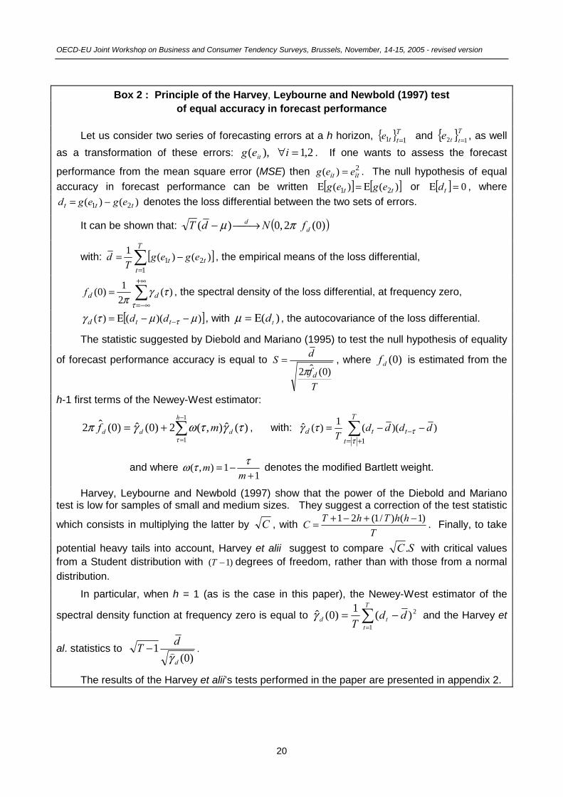
Box 2 : Principle of the Harvey, Leybourne and Newbold (1997) test of equal accuracy in forecast performance
Let us consider two series of forecasting errors at a h horizon, and , as well Ttte 11 = T
tte 12 =
as a transformation of these errors: . If one wants to assess the forecast 2,1),( =∀ieg it
performance from the mean square error (MSE) then . The null hypothesis of equal 2)( itit eeg =accuracy in forecast performance can be written or , where [ ] [ ])()( 21 tt egeg Ε=Ε [ ] 0=Ε td
)()( 21 ttt egegd −= denotes the loss differential between the two sets of errors.
It can be shown that: ( ))0(2,0)( dd fΝdT πµ ⎯→⎯−
with: [=
−=T
ttt egeg
Td
121 )()(1 ] , the empirical means of the loss differential,
+∞
−∞=
=τ
τγπ
)(21)0( ddf , the spectral density of the loss differential, at frequency zero,
[ ]))(()( µµτγ τ −−Ε= −ttd dd , with , the autocovariance of the loss differential. )( tdΕ=µ
The statistic suggested by Diebold and Mariano (1995) to test the null hypothesis of equality
of forecast performance accuracy is equal to
Tf
dSd )0(ˆ2π
= , where is estimated from the )0(df
h-1 first terms of the Newey-West estimator:
−
=
+=1
1)(ˆ),(2)0(ˆ)0(ˆ2
h
ddd mfτ
τγτωγπ , with: +=
− −−=T
tttd dddd
T 1))((1)(ˆ
τττγ
and where 1
1),(+
−=m
m ττω denotes the modified Bartlett weight.
Harvey, Leybourne and Newbold (1997) show that the power of the Diebold and Mariano test is low for samples of small and medium sizes. They suggest a correction of the test statistic
which consists in multiplying the latter by C , with T
hhThTC )1()/1(21 −+−+= . Finally, to take
potential heavy tails into account, Harvey et alii suggest to compare SC . with critical values from a Student distribution with degrees of freedom, rather than with those from a normal )1( −Tdistribution.
In particular, when h = 1 (as is the case in this paper), the Newey-West estimator of the
spectral density function at frequency zero is equal to =
−=T
ttd dd
T 1
2)(1)0(γ and the Harvey et
al. statistics to )0(
1d
dTγ
− .
The results of the Harvey et alii’s tests performed in the paper are presented in appendix 2.
20
Individual responses to BTS and the Forecasting of Manufactured Production...
Stage 2: Dynamic models
The simple regression models used at the first stage of the out-of-sample analysis are, however, not very representative of the kinds of forecasting models of manufacturing production growth that are used in operational short-term forecasting. The latter models generally combine the dynamic effects of several indicators, notably those of the balances of opinion relating to past and expected production36. At the second stage of the out-of-sample analysis, therefore, we consider dynamic forecasting models of manufactured production growth whose formulations are closer to those of operational models.
First, we estimate the eight MSW indicators (the same four kinds of indicators as before, calculated for the two same questions) on sub-period , with t between and (
1,...,1 −t 0T 1−T37, 38). The values of these indicators outside sub-period can be inferred from these
estimations for the total period [ , the crucial point being that the set of (macro or sectoral) observations is not involved in their calculation on the sub-period [ . We also
calculate the two balances of opinion, whose derivation is totally independent from the values of x at any time. Let and denote, respectively, the resulting indicators of a given kind relating to past and expected production.
1,...,1 −t]T,1
( ) 1,...,1 −∉ tx ττ ]Tt,
PInd _ EInd _
Second, we estimate five dynamics models (one per kind of indicators) formulated as follows, again on sub-period : 1,...,1 −t
ττττττ ucEIndbEIndbPIndaPIndax +++++= −−− 1102211 ____
where index τ denotes the current quarter (in the sense of our convention explained in sub-section 4.1 above) and x refers to the manufacturing production growth rate exclusively39. From each of the models estimated on period , and using the values of the indicators at quarter
1,...,1 −tt , we derive a forecast tx~ of for the current quartertx 40. We, then, calculate the
forecasting error = - te tx tx~ at quarter .t
36 On French data see, for instance, Reynaud and Scherrer (1996) or Dubois and Michaux (2005). 37 The model used here is dynamic. Consequently, we can no longer proceed as we did in the first stage
of the out-of-sample analysis. 38 The starting quarter is the first quarter of 1999. When the empirical work was carried out, the last
available quarter in the quarterly accounts, T, was the fourth quarter of 2004. 0T
39 We have carried out the same analysis with two-lag models. The qualitative results are unchanged with respect to those derived from the models with one lag.
40 At the end of July, for instance, the firms’ responses until the July survey are available, as well as the quarterly accounts until the second quarter of the current year. We forecast the third quarter of the accounts (xt) from the model, using the most recent piece of information, derived from the last survey (encompassed in Ind_Pt-1 and Ind_Et) and the survey before (encompassed in Ind_Pt-2 and Ind_Et-1). The lagged time indices of the Ind_P terms stem from the time convention used - cf. sub-section 4.1.
21

OECD-EU Joint Workshop on Business and Consumer Tendency Surveys, Brussels, November, 14-15, 2005 - revised version
We replicate these operations for every quarter t between and T and we, finally, obtain five series of forecasting errors at a one-quarter horizon on the sub-period 1999q2 -2004q4. The comparison of the five series of errors gives some interesting piece of information on the way the five kinds of indicators might perform in the context of the forecasting exercises carried out by short-term analysts. We perform systematic tests of equal accuracy in forecast performance, although the conclusions of the latter tests may be made fragile due to the relatively low underlying number of observations (23).
0T
Before presenting the results in details, note that, as far as the MSW parametric indicator is concerned, we need to estimate the distribution density function of the manufacturing production growth rate . The shapiro-Wilk normality test leading to a clear acceptance of the normal distribution, we choose a normal density function. Last, note that we used the softwares SAS and R.
f
tx
5. Application to the INSEE Industry survey: Results
5.1 In-sample results:
The “macro” and “sector-based” MSW indicators are calculated as indicated in the previous sections, as well as the traditional balances of opinion. The ten indicators are presented, after standardization, in Figures 2 below. In the case of the retrospective question, the correlation between the manufacturing production quarterly growth rate and the balance amounts to 71 %. When replacing the balance with the “macro” non-parametric MSW indicator or, equivalently, the “macro” parametric MSW indicator, the correlation increases up to 86% (85% respectively). The corresponding correlations calculated using the “sector-based” non-parametric and parametric MSW indicators amounts to 86 % (84 % respectively). In the case of the question relating to expected production, the correlation between the manufacturing production quarterly growth rate and the balance is equal to 64%. When replacing the balance with the “macro” non-parametric or parametric MSW indicator, or, alternatively, the “sector-based” non-parametric or parametric MSW indicator, we obtain the following correlations, respectively: 86 %, 87 %, 88 % and 86 %.
These results express that the fluctuations of the MSW indicators are closer to those of the manufacturing production growth rate than those of the balances of opinion on the estimation period. This in-sample property results from the estimation method of the considered indicators, the balances, unlike the MSW indicators, being calculated without any reference to the account aggregate. Only the results of the out-of-sample analysis can tell us whether the MSW indicators perform better than the balances of opinion in terms of the short-term forecasting of the manufacturing production growth rate.
22

Individual responses to BTS and the Forecasting of Manufactured Production...
Figures 2 : The ten standardized indicators (estimated on the whole period)
Past production
-3
-2
-1
0
1
2
3
1990 1992 1994 1996 1998 2000 2002 2004
Balance of opinion
Macro MSWPI
Macro MSWNPI
manufacturingproduction growth rate
Past production
-3
-2
-1
0
1
2
3
Balance of opinion
Sector-based MSWPI
Sector-based MSWNPI
manufacturingproduction grow th rate
Expected production
-3
-2
-1
0
1
2
3
1990 1992 1994 1996 1998 2000 2002 2004
Balance of opinion
Macro MSWPI
Macro MSWNPI
manufacturing productiongrow th rate
Expected production
-3
-2
-1
0
1
2
3
1990 1992 1994 1996 1998 2000 2002 2004
Balance of opinion
Sector-based MSWPI
Sector-based MSWNPI
manufacturingproduction growth rate
Sources: INSEE, Industry survey and quarterly accounts. Calculations by the authors. In the first two figures, the series relating to the indicators are shifted by one quarter so that each account quarter lines up with the reference period of the question on past production. Therefore the first two figures end one quarter earlier than the last two figures.
23
OECD-EU Joint Workshop on Business and Consumer Tendency Surveys, Brussels, November, 14-15, 2005 - revised version
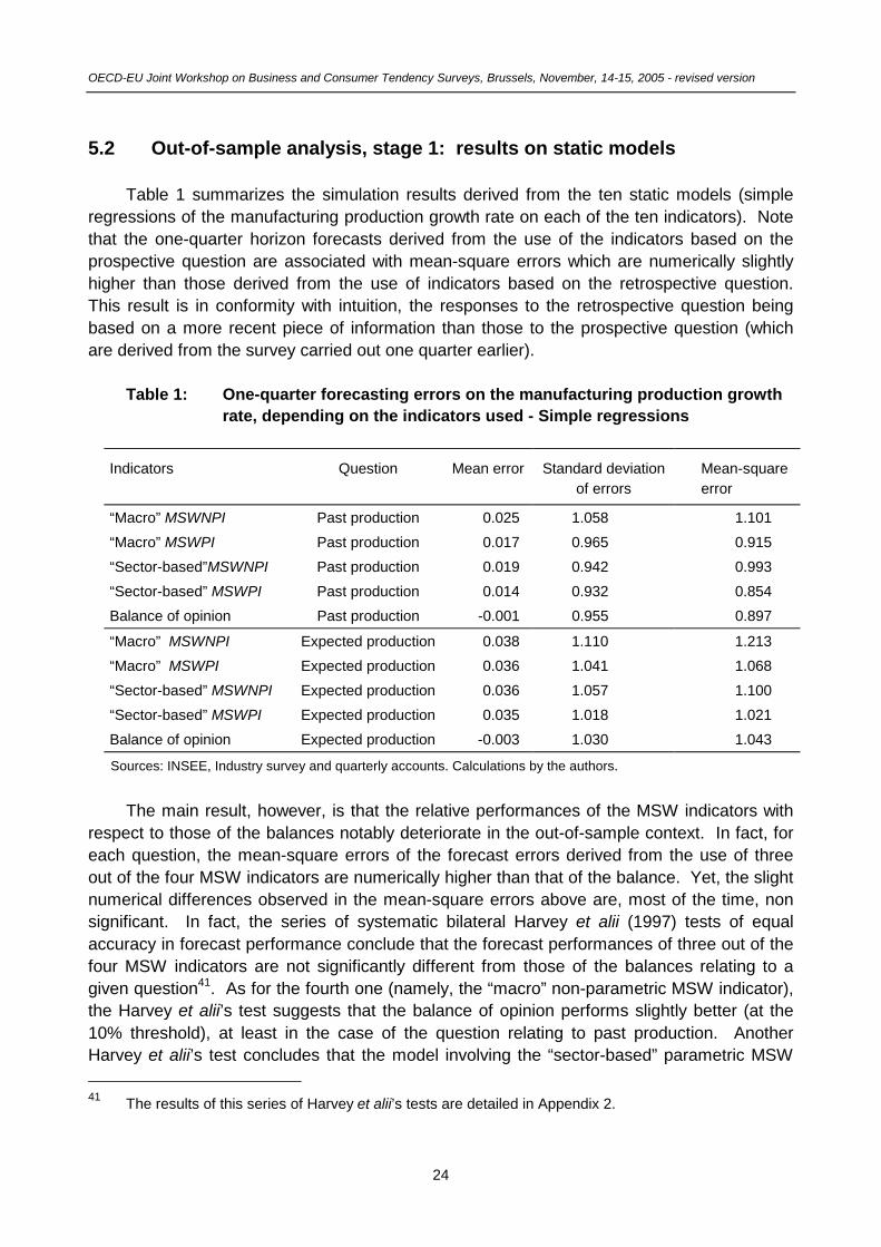
5.2 Out-of-sample analysis, stage 1: results on static models
Table 1 summarizes the simulation results derived from the ten static models (simple regressions of the manufacturing production growth rate on each of the ten indicators). Note that the one-quarter horizon forecasts derived from the use of the indicators based on the prospective question are associated with mean-square errors which are numerically slightly higher than those derived from the use of indicators based on the retrospective question. This result is in conformity with intuition, the responses to the retrospective question being based on a more recent piece of information than those to the prospective question (which are derived from the survey carried out one quarter earlier).
Table 1: One-quarter forecasting errors on the manufacturing production growth rate, depending on the indicators used - Simple regressions
Indicators Question Mean error Standard deviation of errors
Mean-square error
“Macro” MSWNPI Past production 0.025 1.058 1.101 “Macro” MSWPI Past production 0.017 0.965 0.915 “Sector-based”MSWNPI Past production 0.019 0.942 0.993 “Sector-based” MSWPI Past production 0.014 0.932 0.854 Balance of opinion Past production -0.001 0.955 0.897
“Macro” MSWNPI Expected production 0.038 1.110 1.213 “Macro” MSWPI Expected production 0.036 1.041 1.068 “Sector-based” MSWNPI Expected production 0.036 1.057 1.100 “Sector-based” MSWPI Expected production 0.035 1.018 1.021 Balance of opinion Expected production -0.003 1.030 1.043
Sources: INSEE, Industry survey and quarterly accounts. Calculations by the authors.
The main result, however, is that the relative performances of the MSW indicators with respect to those of the balances notably deteriorate in the out-of-sample context. In fact, for each question, the mean-square errors of the forecast errors derived from the use of three out of the four MSW indicators are numerically higher than that of the balance. Yet, the slight numerical differences observed in the mean-square errors above are, most of the time, non significant. In fact, the series of systematic bilateral Harvey et alii (1997) tests of equal accuracy in forecast performance conclude that the forecast performances of three out of the four MSW indicators are not significantly different from those of the balances relating to a given question41. As for the fourth one (namely, the “macro” non-parametric MSW indicator), the Harvey et alii’s test suggests that the balance of opinion performs slightly better (at the 10% threshold), at least in the case of the question relating to past production. Another Harvey et alii’s test concludes that the model involving the “sector-based” parametric MSW 41 The results of this series of Harvey et alii’s tests are detailed in Appendix 2.
24

Individual responses to BTS and the Forecasting of Manufactured Production...
indicator performs better (at a threshold of 5% or 10%, depending on the cases) than the models using the other MSW indicators. Therefore, the estimation of the MSW parametric indicator at a more broken-up sectoral level might have a slightly positive effect, but not strong enough to allow for a significant improvement with respect to the forecast performance of the corresponding balance of opinion. Unlike MSW (2002, 2004, 2005) we, thus, find that the non-parametric indicators do not perform better than the parametric indicators, quite the contrary. The big size of the French panel might constitute a favorable context for the use of the parametric indicators with respect to that of the non-parametric ones.
All in all, this first out-of-sample analysis suggests that the MSW indicators do not enable us to anticipate the manufacturing production growth rate better than the corresponding balance of opinion at a one-quarter horizon. The relative forecast performances of the MSW indicators, thus, appear to be notably weakened when they are used outside their estimation period. The balances of opinion, whose calculation is much simpler and totally independent of the aggregate to forecast, finally seem at least as liable to anticipate this aggregate.
Note that the difference between the in-sample and out-of-sample results may not appear quite intuitive at first sight. In fact, one could expect the message given by simple regressions to be close to that derived from simple correlations. This is not the case due to the significant differences between the values of the MSW indicators at quarter t derived from the in-sample calculations on period [ on the one hand and from the out-of-sample calculation on the basis of the estimation on period [ ] \ on the other hand - see figure 3 for an illustration.
]T,1T,1 t
Figure 3: The “macro” parametric MSW indicator relating to past production estimated on the whole period and the “simulated MSW indicator”
-3
-2
-1
0
1
2
MSW macro indicator (resulting from the in-sample estimation)
Simulated MSW macro indicator (derived from the 1st-stage out-of-sample analysis)
Sources : INSEE Industry survey and French Quarterly Accounts. Calculations by the authors. The value of the “simulated MSW indicator” at time t is obtained by calculating the macro parametric MSW indicator at time t on the basis of the estimation performed on period [1,T]\t.
25

OECD-EU Joint Workshop on Business and Consumer Tendency Surveys, Brussels, November, 14-15, 2005 - revised version
Finally, the relatively high mean-square errors derived from using either one indicator or the other deserve a brief comment. As table 1 illustrates, the forecasts are unbiased on average (mean errors close to zero), especially those derived from models involving the balances, but the standard deviations of the forecasting errors are fairly high with respect to the order of magnitude of the aggregate of interest (expressed in percents). This reflects the fact that BTS indicators are notably smoother than the macroeconomic aggregates from the quarterly accounts (see below, sub-section 5.3).
5.3 Out-of-sample analysis, stage 2: results on dynamic models
The simulation results derived from the second stage of the out-of-sample analysis suggest a superiority of the model involving the two balances of opinion as concerns the one-horizon forecasting of the manufacturing production growth rate (see table 2, figures 4 and Appendix 2). Harvey et alii’s tests confirm the superiority of the balances over the four MSW indicators (cf. appendix 2, tables A2.3).
A possible explanation for the better performances of the balances of opinion relatively to the MSW indicators at the second stage of the out-of-sample analysis (to be compared with their similar performances with respect to most MSW indicators at the first stage) might stem from the lower number of observations on which the dynamic analysis is based. On the one hand, the shorter estimation periods might intuitively favor the simplest and more parsimonious kinds of indicators, namely the balances of opinion. On the other hand, the lower length of the simulation period at the second stage of the out-of-sample analysis (23 observations instead of 60 at the first stage) might lead to more fragile results, especially if the simulation period proves to be relatively specific. However, one cannot exclude the occurrence of a “model” effect (more convincing dynamic models might enable us to better discriminate the relative performances of the studied indicators).
Besides, the simulations of the manufacturing production growth rate derived from the dynamic models seem to lead to less accurate forecasts than those derived from the simple regressions, despite the use of more convincing dynamic models, which appears to be somewhat paradoxical at first sight. In fact, the mean-square errors in table 2 are a little higher than those in table 1, essentially due to the existence of negative biases on the period (of around -0.3 point, i.e. of the same order of magnitude as the macroeconomic aggregate of interest). Here, again, several possible causes can be involved.
26

Individual responses to BTS and the Forecasting of Manufactured Production...
Table 2: One-quarter forecasting errors on the manufacturing production growth rate, depending on the indicators used - Dynamic models
Indicators Mean error Standard-deviation of errors Mean-square error
“Macro”MSWNPI -0.382 1.105 1.315 “Macro” MSWPI -0.263 1.073 1.172 “Sector-based”MSWNPI -0.448 1.138 1.438 “Sector-based” MSWPI -0.299 1.110 1.267 Balances of opinion -0.419 0.762 0.732
Sources: INSEE, Industry survey and quarterly accounts. Calculations by the authors.
Figures 4 : One-quarter forecasting errors on the manufacturing production growth rate derived from the dynamic models
-3
-2
-1
0
1
2
1999 2000 2001 2002 2003 2004
Balances of opinion Macro MSWNPI Macro MSWPI
-3
-2
-1
0
1
2
1999 2000 2001 2002 2003 2004
Balances of opinion Sector-based MSWNPI Sector-based MSWPI
Sources: INSEE, Industry survey and quarterly accounts. Calculations by the authors.
A possible way to discriminate, at least partly, the relative impacts of the models used, the length of the estimation period, and the specific feature of both the estimation and simulation periods is to restrict the study of the forecast errors derived from the simple regressions to the sub-period 1999q2 - 2004q4 on which the second-stage out-of-sample analysis has been carried out. The results of the first-stage out-of-sample analysis on this sub-period are presented in table 3 below, as well as in tables A2.4 and A2.5, Appendix 2.
27

OECD-EU Joint Workshop on Business and Consumer Tendency Surveys, Brussels, November, 14-15, 2005 - revised version
Table 3: One-quarter forecasting errors on the manufacturing production growth rate, depending on the indicators used: Simple regressions - Results on the sub-period 1999q2 to 2004q4
Indicators Question Mean error Standard deviation of errors
Mean-square error
“Macro” MSWNPI Past production -0.271 1.074 1.177 “Macro” MSWPI Past production -0.023 1.023 1.001 “Sector-based” MSWNPI Past production -0.302 1.031 1.107 “Sector-based” MSWPI Past production -0.108 0.985 0.939 Balance of opinion Past production -0.174 1.001 0.989
“Macro” MSWNPI Expected production -0.355 1.151 1.394 “Macro” MSWPI Expected production -0.096 1.107 1.181 “Sector-based” MSWNPI Expected production -0.358 1.146 1.384 “Sector-based” MSWPI Expected production -0.167 1.097 1.179 Balance of opinion Expected production -0.278 0.985 1.005
Sources: INSEE, Industry survey and quarterly accounts. Calculations by the authors.
At the 5% threshold, the Harvey et alii tests confirm that, on the sub-period 1999q2 - 2004q4 (table 3) as well as on the whole period (table 1), the average forecast performances of the MSW indicators, when used in the simple regressions, do not significantly differ from that of the corresponding balance of opinion. On the sub-period 1999q2 - 2004q4, the balance relating to the prospective question seems to perform slightly better than the non-parametric indicators at the 10% threshold. Nonetheless, on the whole, the results of the first-stage out-of-sample analysis are not notably modified when focusing on the sub-period 1999q2 - 2004q4, at least as concern the relative forecast performances of the five kinds of indicators. In this respect, it seems that the “model” effect predominates, the combination of the indicators relating to past and expected production within the more convincing dynamic models leading to a diagnosis more clearly in favor of the balances.
Moreover, unlike table 1, table 3 shows frequent negative forecast biases, although less notable as in table 2. In this respect, there might also be a slight “model” effect, but which does not seem to predominate. Here, the problem is probably due to the fact that, the shorter the simulation period, the more dependent on the specific characteristic features of the simulation period. The sub-period 1999q2 - 2004q4 contains the beginning of the years 2000, as well as the year 2004, during which the French BTS suggested somewhat higher growth rates than those published in the quarterly accounts.
All in all, the quasi-systematic occurrences of negative forecast biases in tables 2 and 3 do not mean that BTS cannot be used for the short-term forecast of the manufacturing production growth rate in general, as the absence of significant systematical biases in the first set of forecasts based on longer estimation and simulation periods illustrates (table 1). Nonetheless, it is true that, at certain periods (such as in the beginning of the years 2000 or
28

Individual responses to BTS and the Forecasting of Manufactured Production...
in 2004), the BTS and the quarterly accounts may not lead to perfectly consistent assessments on economic activity. Often, the magnitude of the gap tends to decrease as time goes by, due to the successive revisions in the national accounts; but some discrepancies may remain, punctually leading to significant forecast errors. More generally, the main short-term divergences between the economic assessments given by the BTS on the one hand and by the quarterly accounts on the other hand stem from the smoother characteristic feature of the BTS series. This explains the relatively high standard deviations of the forecast errors derived from the calibration models studied, whatever the models used and the simulation period. The BTS remain, however, very useful tools for the short-term forecasting of economic activity, in the sense that they enable one to assess the general tendencies of its inflexions relatively well, if not always the large magnitude of some of its variations.
6. Conclusions and perspectives
6.1 Five empirical applications, disparate findings
MSW (2002, 2004) elaborate two kinds of short-term dis-aggregate indicators: a parametric one based on ordered discrete-choice models at the firm level (logit polytomic models), and a non-parametric one based on a simpler methodology. Their successive empirical applications conclude that these dis-aggregate indicators perform better than a set of three benchmark aggregate indicators on British and German data, but not on Portuguese and Swedish data. As far as the two latter countries are concerned, however, the more striking aspect of the results is the very high mean-square errors of the forecast errors obtained, whatever the indicator used, in correlation with the extremely small size of the available panels. In this context, the performance gaps from one indicator to another appear to be of minor interest. Consequently, our further comments will focus on the results (in favor of the dis-aggregate indicators) obtained by MSW (2004-2) from the two panels of more reasonable size, namely those of Germany and the UK, to be compared with the results of the present paper.
In the latter, we present an application on French data, where we compare the short-term performances of five kinds of indicators: an aggregate indicator (the balance of opinion), and four dis-aggregate indicators based on the MSW (2002, 2004-1) methodology. We derive these indicators from the entrepreneurs’ responses to two questions asked in the INSEE Industry survey and the manufacturing production growth rate derived from the French quarterly accounts, thus obtaining ten indicators. We, then, study the latter indicators’ in-sample correlations with the manufacturing production output growth rate, as well as their out-of-sample properties as regard their relative performances in terms of the one-horizon forecasting of the same macroeconomic aggregate.
In this respect, our main conclusion is that the balances of opinion perform better or, at least, as well as the four MSW indicators. Although not reproducing the exact methodology of MSW (2002, 2004, 2005), our paper therefore suggests that the promising results obtained
29

OECD-EU Joint Workshop on Business and Consumer Tendency Surveys, Brussels, November, 14-15, 2005 - revised version
by MSW (2004-2) on British and German data do not seem to be easily generalized to all EU Member States. Besides, unlike MSW’s application on British data, we find that the MSW parametric indicators perform slightly better than the MSW non-parametric indicators. Last, our results suggest that “sector-based” indicators should be preferred to indicators directly estimated at the total manufactured industry level.
As was already mentioned, part of the divergences between MSW’s findings and ours is probably due to the size of the French panel, which is notably bigger than those of MSW’s panels. In fact, intuitively, numerous observations constitute a relatively more favorable estimation context for the (more complex) MSW parametric indicators than for the (simpler and more parsimonious) MSW non-parametric indicators, while the opposite configuration tends to favor the latter to the expense of the former indicators. This intuition is supported by the fact that we find more performing parametric indicators on the (biggest) French panel, while MSW obtain more performing non-parametric indicators on the (smaller) British panel and non-significant difference in forecast accuracy between the two dis-aggregate indicators on the German panel (whose size is probably intermediate between those of the British and the French panels).
As for the relative performances of the aggregate indicators on the one hand, and the dis-aggregated ones on the other, it might be difficult to compare MSW’s findings to ours, due to the fact that the aggregate indicators considered in the two sets of applications differ. However, as was briefly mentioned previously, it turns out that the “regression” approach applied to the French data leads to a Pesaran indicator that does not significantly differ from an affine function of the balance of opinion, for both the retrospective and the prospective questions. In fact, when we estimate the model: , where U and D denote the (appropriately weighted
tttt uDUx ++−= χβα42) proportions of elementary units that reported “up” and
“down”, respectively, u the error term, and α, β and χ unknown coefficients, we find that the null hypothesis of coefficients α and β of equal magnitude and opposite signs is clearly accepted for both questions43. The balances in the French application can, therefore, be seen as homogenous to Pesaran indicators. Consequently, the opposition between the MSW results and ours in terms of aggregate versus dis-aggregate indicators’ forecast accuracy cannot be seen as an artifact originating from the differences in the sets of indicators.
42 Using the same double-weighting scheme as for the balances of opinion. 43 Consequently, the Pesaran indicator, defined as: , where and χβα ˆˆˆ +−= ttt DUPI βα ˆ,ˆ χ are
the OLS estimators of α, β and χ, does not significantly differ from χα ~)(~ +−= ttt DURPI , where α~ and χ~ are the restricted estimators of α and χ under the null hypothesis: H0 : α + β = 0, and
is the balance of opinion. )( tt DU −
30
Individual responses to BTS and the Forecasting of Manufactured Production...
Admittedly, no clear explanation for this opposition clearly arises from differences in data periodicity44, estimation period45 or panel size46. Moreover, it is difficult to assess any structural difference from one country to another47. In any case, it seems to us that the findings from the French application raise more questions on the forecast performance of the MSW dis-aggregate indicators than those derived from Portugal and Sweden, as the size of the French panel is big enough to assure a better robustness of the results. Are the sizes of the British and German panels large enough to assure a sufficient robustness of MSW’s findings on these country data? We do not have enough pieces of information in this respect to be able to conclude without doubt in this respect.
Besides, we cannot exclude a possible impact of differences in methodology, although that used by MSW in their most recent applications tends to be much closer to ours than their former one, without any qualitative change in the results. Yet, the indicators’ weighting schemes, might be of some importance. The French balances of opinion benefit from a double weighting scheme, which may not be the case for the Pesaran indicator in MSW (2004-2). Moreover, in our study, the “sector-based” MSW indicators tend to perform fairly better than the “macro” MSW indicators. This result may stem from the more broken-up production growth rates used in the estimations performed at the individual level in the case of the “sector-based” MSW indicators, but also from the differences in weighting schemes between the two kinds of MSW indicators. In this respect, it is very difficult to isolate the two possible effects, which are tightly linked, as the sectoral weighting scheme used for the “sector-based” MSW indicators is consistent with the sector level at which their components are estimated. Correlatively, the reason why the “sector-based” methodology leads to a slight improvement is not clear. This may originate from the correction of a small selection bias due to uneven non-response rates between sectors, in a configuration when the sectoral representativeness of the responses matters, for instance because the responses of the firms are subject to a “standpoint bias”48, or due to a structure effect or both, the two contexts not being mutually exclusive, quite the contrary. For example, a structure effect may happen due
44 The French application, like the German one, is based on quarterly data, while the British one is
based on monthly data, with no clear consequences in terms of the results. 45 Those of the three applications are close, although not identical: 1990-2004 for France, 1991-2000 for
Germany, 1988-1999 for the UK. In particular, the first half of the 2000s, whose relative specificity as for the French application has been mentioned in sub-section 5.3, is absent from the other panels.
46 Intuitively, the big size of the French panel should relatively favor the more complex methodologies, which seems to be the case within the sub-set of MSW indicators; but the balances of opinion, based on a much simpler methodology than the parametric MSW indicators, perform better or, at least, as well. Conversely, in the smaller British and German samples, the parametric MSW indicators outperform the, simpler, Pesaran indicators.
47 Within the covered period, business cycles in France and Germany are closer to one another than to those in the UK. It is not clear, however, whether this should have a significant impact on the relative forecast performances of the aggregate and dis-aggregate indicators. At all events, the results do not tell us anything that tends to support this possibility (even though they cannot be considered to prove the contrary).
48 Cf. above, sub-section 4.2.1 for a definition.
31

OECD-EU Joint Workshop on Business and Consumer Tendency Surveys, Brussels, November, 14-15, 2005 - revised version
to differences between sectors in terms of degree of concentration and average size of firms, if bigger firms are better informed on the macroeconomic aggregate of interest than smaller firms49. In this configuration (which might not be unrealistic), a weighting scheme by firm size would be liable to lead to a better performing indicator. This is the case for the balances and, indirectly and to a lesser extent, for the sector-based MSW indicators, but not for the “macro” MWS indicators. Although we do not have much information available on firms’ response behavior (depending on sector and size, notably), the results we obtain, at least, do not contradict the possible occurrence of such configurations. Consequently, even though, in principle, the MSW indicators, unlike balances, do not need being weighted by firm size, it might be interesting to extend the present study with the introduction of MSW indicators whose weighting scheme be more similar to those of the balances, either fully (if firm size is supposed to influence the quality of responses) or partly (at the strata level for instance, if strata representativeness matters for another reason than because of firm size). Remember, however, that MSW (2004-2) find that the equal weighting scheme outperforms the weighting scheme by firm size (which influenced our choice of privileging fully or partly non-weighted MSW indicators). Therefore, the issue of the weighting scheme remains open, and the possible interpretations envisaged here are uncertain and would need being tested. All in all, like MSW (2004-2), we consider that the weighting aspect deserves further research (see below, 6.3).
6.2 Balances of opinion versus MSW dis-aggregate indicators, beyond their exclusive use for short-term forecasting of activity
At this stage of our analysis on French data, the tested dis-aggregate MSW indicators have not outperformed the balances of opinion in terms of short-term forecasting of activity. In the light of our empirical experience on the computing of the MSW dis-aggregate indicators, it seems to us that, beyond the specific issue of forecasting, the balances show clear advantages over the MSW dis-aggregate indicators:
1. The estimation of the MSW parametric indicators is quite long in terms of calculation time, even when focusing on the responses to one question only. Conversely, the simple and rapid calculation of the balances relating to a whole survey constitutes a crucial advantage for operational use;
2. The calculation of the MSW indicators requires a relatively high number of observations per firm, which leads to the exclusion of the less good-responding firms’ answers. Consequently, a notable number of observations are eliminated from the calculation of the dis-aggregate indicators. This may raise a statistical issue, as far as both the degree of exhaustiveness of the MSW indicators and the potential existence of
49 A specific case might be that smaller firms be more subject to a “standpoint bias” than the bigger
firms.
32
Individual responses to BTS and the Forecasting of Manufactured Production...
selection bias are concerned50,51. Balances of opinion, conversely, are calculated on the basis of a significantly higher number of observations, which limits the risks for both loss in exhaustiveness and selection bias.
3. Balances of opinion are subject to low revisions, if not to no revisions at all, depending on the survey producers’ methodologies52. Conversely, the MSW indicators may experience significant revisions from one quarter to another, partly because every reestimation affects the whole series. Above all, the strong sensitivity of the MSW indicators to the manufacturing production growth rate, itself subject to significant revisions, may induce notable revisions in the “macro” and “sector-based” MSW indicators.
4. This very sensitivity of the MSW indicators to the manufacturing production growth rate derived from the quarterly accounts, which is noticeably less smooth than the balances of opinion, also affects the profile of the dis-aggregate indicators, which tend to be slightly less smooth than the corresponding balances.
All these relative properties of the considered indicators tend to weigh in favor of the balances of opinion. Yet, the present study by no means puts an end to the issue of the best possible combination of the individual responses to BTS, quite the contrary. Many tracks for future research remain to be explored.
6.3 Tracks for future research
First, as was discussed above, the issue of the indicators’ weighting schemes deserves further research. A natural way of extending the present work would be to study the impact of two additional weighting schemes on the indicators’ relative performances:
- one by strata size, either without changing the estimation level (“macro” or sectoral”), just to limit potential selection biases that might occur in the data if strata representativeness matters (for reasons to be discussed), or together with the application of the “sector-based” MSW indicators methodology at a more broken-up level (see below);
- another by firm size, reproducing the double-weighting scheme of the balances, under the assumption that firm size is correlated with the quality of individual macro-economic or sectoral forecasts. An improvement in the relative performances of the MSW indicators would support this assumption.
50 Even if MSW (2004-2)’s empirical checks in this respect do not point any striking sign for the
existence of such biases. 51 The use of “sector-based” indicators may limit this possible bias if the conditions justifying the use of
unequal weighting schemes are satisfied (cf. discussion on the impact of the weighting scheme above, sub-section 6.1).
52 In the case of the INSEE surveys, only the next to last observations of gross balances, at most, are revised from one release to the next, and the magnitudes of the revisions are rather limited in general.
33
OECD-EU Joint Workshop on Business and Consumer Tendency Surveys, Brussels, November, 14-15, 2005 - revised version
Beyond the issue of the indicators’ weighting scheme, there remains some room for further tests and improvements in the direct line of the present study, especially as concern the parametric indicators.
- The parametric indicators relating to the expected question could be theoretically improved by applying the MSW (2005) correction for potential endogeneity problems.
- It might be interesting to test whether the performances of the parametric indicators would remain unchanged if the analysis was performed on a sub-panel involving the firms’ responses relating to one main product exclusively. Theoretically, the assumption of independently distributed error terms in model (6) would, then, be less subject to caution. Conversely, the drop in the number of observations might lead to a deterioration in the performances of the parametric indicators. However, the relatively low number of products declared per firm (1.3 on average in the selected panel) makes it little likely that this test should induce notable changes in the results.
- One could try not to include the responses of atypical firms by introducing a condition on the sign of the estimated value of coefficient in model (6). This might modify the results as the number of firms for which this estimated coefficient is negative or non significantly different from zero is negligible neither in the MSW applications, nor in ours - cf. Appendix 3. However, it is not clear whether one should systematically eliminate atypical firms, whose responses may encompass an interesting piece of information on macroeconomic activity.
iβ
- One could slightly modify model (6) in order to make it become more convincing from an economic point of view. A possible track would be to adjust the model in order to make it possible that certain firms experience more dynamic growth whatever the position of the economy in the cycle. This configuration is not allowed in model (6). In fact, the term in the right member of equation (6) assumes that the firms whose production increases faster than the average (represented by the manufacturing production growth rate ) when the position in the cycle is high ( ) also experience more rapid decline in phases of negative overall growth ( ). This property of model (6) does not seem to be very convincing, which suggests preferring a variant version of the model:
, where equals unity if and zero otherwise, and . However, such a modification would not compulsorily lead to an improvement in the MSW parametric indicators. First, the question can be raised whether the threshold of zero would optimally define the high positions in the cycle (first dummy variable). Second, the introduction of an additional unknown coefficient would make the elaboration of the parametric indicators still more demanding in terms of number of observations. The risk exists that this might lead to less robust results.
ti xβ
tx1>iβ0<tx
tixixiiti tty ,)0()0(, εββα +++= <−≥+ 11 )0( ≥tx1 0>tx
)0()0( 1 ≥< −=tt xx 11
34

Individual responses to BTS and the Forecasting of Manufactured Production...
All in all, despite the intuition that the elaboration method of the MSW parametric indicators could be improved, it is not certain, however, that the above described tracks for future research would lead to more performing parametric indicators.
Another possible track would be to try to add indicators of variability of the individual responses to the survey directly in the list of explanatory variables of the short-term forecasting models of activity, in combination with indications on the direction of responses’ changes. The underlying intuition here is that an increasing variance of the individual perceptions might be considered to proxy the degree of uncertainty in the economy, which rises before an inflexion or a turning point53.
Last but not least, for a country like France, for which infra-annual quantitative survey data are available on industrial firms’ production, it would be interesting to compare the responses given by firms to the qualitative BTS and to the quantitative surveys. This might enable one to elaborate more convincing forecasting models of the manufacturing production growth rate involving the two sources. Quantitative surveys would also enable one to apply the principle of the “sector-based” MSW indicators at a much broken-up level, using the so-called “elementary industrial production indices” derived from the individual responses to the quantitative surveys, instead of the sectoral production growth rates from the quarterly accounts. We plan to carry out this kind of study in a close future.
53 This track for future research can be linked to previous work by Zarnowitz and Lambros (1987), Lahiri,
Teigland and Zaporowski (1988), and many others, even though the context is not exactly the same (most of this literature focusing on inflation expectations).
35
OECD-EU Joint Workshop on Business and Consumer Tendency Surveys, Brussels, November, 14-15, 2005 - revised version
References
Amemiya, T. (1985), Advanced Econometrics, Basil Blackwell.
Anderson, O. (1952), The business test of the IFO-Institute for Economic Research, Munich, and its theoretical model, Revue de l’Institut International de Statistique, vol. 20, 1-17.
Ashley R. (1993), Statistically significant forecasting improvements: How much out-of-sample data is likely necessary, International Journal of Forecasting, vol. 19, 229-239.
Balcombe K. (1996), The Carlson - Parkin method applied to NZ price expectations using QSBO survey data, Economic Letters, vol. 15., 51-57.
Batchelor, R.A. (1981), Aggregate expectations under the stable laws, Journal of Econometrics, vol. 16, 199-210.
Batchelor, R.A., Orr A.B. (1987), Inflation expectations revisited, Economica, vol. 55, 317-331.
Bengoechea P., Pérez-Quirós G. (2004), A useful tool to identify recessions in the Euro area, Documentos de trabajo, n. 0419, Banco de España, and European Economy, Economic Papers n. 215, October.
Berk J. (1999), Measuring inflation expectations: A survey data approach, Applied Economics, vol. 31, n. 11, 1467-1480.
Bouton F., Erkel-Rousse H. (2002), Conjonctures sectorielles et prévision à court terme de l’activité : l’apport de l’enquête de conjoncture dans les services, Economie et Statistique, numéro spécial « Analyse conjoncturelle : entre statistique et économie », n°359-360, 35-68. English version: Sectoral business surveys as an aid to short-term macroeconomic forecasting: The services’ contribution, 27th CIRET conference, Warsaw, September.
Britton E., Cutler J., Wardlow A. (1999), The Bank’s use of survey data, Bank of England Quarterly Bulletin, May, 177-182.
Carlson J.A. (1975), Are price expectations normally distributed?, Journal of the American Statistical Association, vol. 70, n. 352, 749-754.
Carlson J.A., Parkin M. (1975), Inflation expectations, Economica, 42, 123-138.
Cornec M., Deperraz T. (2005), A monthly indicator of the business climate in the French service industry, Workshop on frontiers in benchmarking techniques and their applications to official statistics, Eurostat, Luxembourg, October 21, paper available on http://epp.eurostat.cec.eu.int/portal/page?_pageid=1853, 19167133,1853_41880052&_dad=portal&_schema=PORTAL.
Cunningham A.W.F., Smith R.J. , Weale M.R. (1998), Measurement errors and data estimation: the quantification of survey data, In Applied Economics and Public Policy (Begg, I. and S.G.B. Henry ed.), Cambridge University Press.
Dasgupta S., Lahiri K. (1992), A Comparative Study of Alternative Methods of Quantifying Qualitative Survey Responses Using NAPM Data, Journal of Business and Economic Statistics, vol. 10, n. 4, 391-400.
D’Elia E. (2005) : Using the results of qualitative surveys in quantitative analysis, Documenti di Lavoro n. 56, ISAE (Istituto di Studi e Analisi Economica), September.
Diebold F. X., Mariano R. S. (1995), Comparing Predictive Accuracy, Journal of Business and Economic Statistics, 13, 253-265.
Doz C., Lenglart F. (1999), Analyse factorielle dynamique : test du nombre de facteurs, estimation et application à l’enquête de conjoncture dans l’industrie, Annales d’Économie et de Statistique, n°54, 91-127. English version (1996): Factor analysis and unobserved component models: an application to the study of French business surveys, INSEE Working paper of the Direction des Etudes et Synthèses Economiques n. 9606, Série rouge.
36

Individual responses to BTS and the Forecasting of Manufactured Production...
Driver C., Urga G. (2004), Transforming qualitative survey data, Performance comparisons for the UK, Oxford Bulletin of Economics and Statistics, vol. 66, n. 1-iv, February, 71-89.
Dubois E., Michaux (2005), Étalonnages à l’aide d’enquêtes de conjoncture : de nouveaux résultats, Economie et Prévision, forthcoming.
European Commission (2004), The joint harmonised EU program of business and consumer surveys, User guide, updated 26/05/2004, available on the European Commission website: http://europa.eu.int/comm/economy_finance/indicators/business_consumer_surveys/userguide_en.pdf
Fansten M. (1976), Introduction à une théorie mathématique de l’opinion, Annales de l’INSEE n.21, janvier-mars 1976, 3-54.
Fishe R.P., Lahiri K. (1981), On the estimation of inflationary expectations from qualitative responses, Journal of Econometrics, vol. 16, 89-102.
Forni M., Hallin M., Lippi M., Reichin L. (2001), Coincident and leading indicators for the Euro area, Economic Journal, 101, 62-75.
Grégoir S., Lenglart F. (2000), Measuring the probability of a business cycle turning point by using a multivariate qualitative hidden Markov model, Journal of Forecasting, n.19, 81-102.
Hamilton J.D. (1989), A new approach to the economic analysis of non stationary time series and the business cycle, Econometrica, 57, 357-384.
Hamilton J.D. (1990), Analysis of time series subject to changes in regimes, Journal of econometrics, vol. 45, 39-70.
Harvey, D.I., Leybourne S.J., Newbold P. (1997), Testing the Equality of Prediction Mean Square Errors, International Journal of Forecasting, vol. 13, 273-281.
Hild F. (2002), Une lecture enrichie des réponses aux enquêtes de conjoncture, Economie et Statistique, numéro spécial « Analyse conjoncturelle : entre statistique et économie », n°359-360, 13-34.
Hild F. (2005), Un nouvel indicateur synthétique prenant en compte la dynamique des réponses individuelles à l’enquête Activité dans l’industrie, Séminaire du Département des Etudes Economiques d’Ensemble, INSEE, 29 juin.
Kaiser U., Spitz A. (2000), Quantification of qualitative data using ordered probit models with an application to a business survey in the German service sector, 25th CIRET conference, Paris, October 10-14.
Lahiri K., Moore, G.H. Eds. (1991), Leading economic indicators: New approaches and Forecasting Records, Cambridge University Press, 464 p.
Lahiri K., Teigland C., Zaporowski M. (1988), Interest rates and the subjective probability distribution of inflation forecasts, Journal of Money, Credit, and Banking, vol. 20, n. 2, May, 233-248.
Lahiri K., Wang J.G. (1994), Predicting turning points with leading index in a Markov switching model, Journal of Forecasting, vol. 13, 245-263.
Lankes F., Wolters J. (1988), Das IFO-Geschäftsklima und seine Komponenten als vorlaufende Indikatoren, Empirische Ergebnisse für die Verbrauchs- und Investitionsgüterindustrie für 1975-1986, FU Berlin, Fachbereich Wirtschaftswissenschaft, Diskussionsarbeit, n. 5/1988 (quoted in D’Elia, 2005).
Lee K.C. (1994), Formation of price and cost inflation expectations in British manufacturing industries: A multisectoral analysis, Economic Journal, vol. 107, 372-386.
Lenglart F., Toutlemonde F. (2002), Mieux appréhender le climat conjoncturel de la zone euro, Economie et Statistique, numéro spécial «Analyse conjoncturelle : entre statistique et économie», n°359-360, 69-82.
Mitchell, J., Smith R.J., Weale M.R. (2002), Aggregate versus Disaggregate Survey-Based Indicators of Economic Activity, mimeo.
37

OECD-EU Joint Workshop on Business and Consumer Tendency Surveys, Brussels, November, 14-15, 2005 - revised version
Mitchell J., Smith, R.J., Weale, M.R. (2002), Quantification of Qualitative Firm-Level Survey Data, Economic Journal, vol. 112, C117-C135.
Mitchell, J., Smith R.J., Weale M.R. (2004-1), Aggregate versus Disaggregate Survey-Based Indicators of Economic Activity, 27th CIRET conference, Warsaw, September.
Mitchell, J., Smith R.J., Weale M.R. (2004-2), The impact of survey aggregation methods on the quality of business survey indicators, Report for the European Commission, ECFIN/2003/A3-04, November.
Mitchell, J., Smith R.J., Weale M.R. (2005), Forecasting manufacturing output growth using firm-level survey data, The Manchester School, vol. 73, Issue 4, 479-499.
Nardo M. (2003), The Quantification of Qualitative Survey Data: A Critical Assessment, Journal of Economic Surveys, vol. 17, n.5, December, 645-668.
Pesaran, M.H. (1984), Expectations formation and macroeconomic modelling, In Contemporary Macroeconomic Modelling (P. Malgrange and P.A. Muet eds.), Blackwell, Oxford.
Pesaran, M.H. (1987), The limits to rational expectations, Basil Blackwell.
Reynaud M., Scherrer S. (1996), Une modélisation VAR de l’enquête de conjoncture de l’Insee dans l’industrie, document de travail de la Direction de la Prévision, n°96-12.
Sargent T.J., Sims C.A. (1977), Business cycle modeling without pretending to have too much a-priori economic theory, in New Methods in Business Cycle Research, ed. Sims and al., Minneapolis: Federal Reserve Bank of Minneapolis, quoted by Stock and Watson (2002).
Smith J., McAleer M. (1995), Alternative procedures for converting qualitative response data to quantitative expectations: an application to Australian manufacturing, Journal of Applied Econometrics, vol. 10, 165-185.
Stock J.H. and M.W. Watson (2002), Macroeconomic forecasting using diffusion indexes, Journal of business and Economic Statistics, 20, 147-162.
Stone J.R.N. (1947), On the interdependence of blocks of transactions, Supplement of the Journal of the Royal Statistical Society, vol. 9, n. 1, 1-32.
Theil, H. (1952), On the time shape of economic microvariables and the Munich business test, Revue de l’Institut International de Statistique, vol. 20, 105-120.
Watchel P. (1977), Survey measures of expected inflation and their potential usefulness, in Analysis of Inflation: 1965-1974, J. Popkin (ed.), NBER, Ballinger, Cambridge (quoted by D’Elia, 2005).
Zarnowitz V., Lambros L.A. (1987), Consensus and uncertainty in economic prediction, Journal of Political Economy, 95, June, 591-621.
38
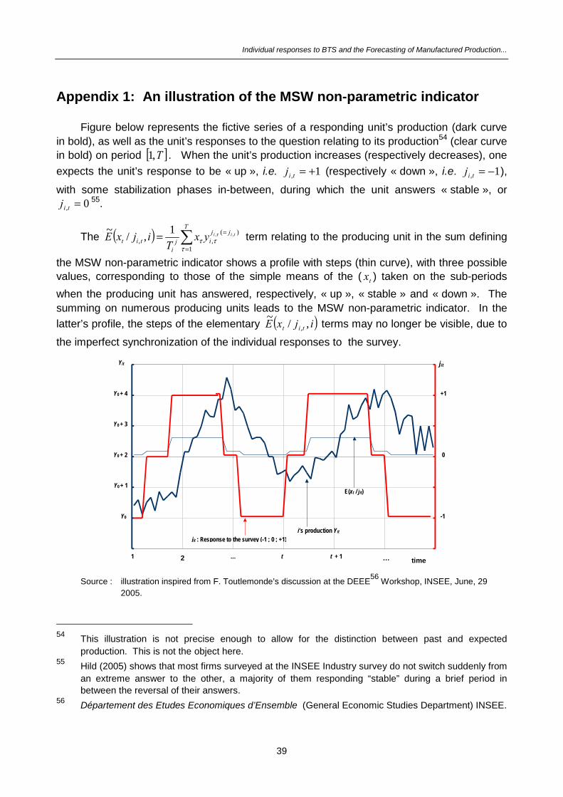
Individual responses to BTS and the Forecasting of Manufactured Production...
Appendix 1: An illustration of the MSW non-parametric indicator
Figure below represents the fictive series of a responding unit’s production (dark curve in bold), as well as the unit’s responses to the question relating to its production54 (clear curve in bold) on period . When the unit’s production increases (respectively decreases), one expects the unit’s response to be « up », i.e. (respectively « down », i.e. ), with some stabilization phases in-between, during which the unit answers « stable », or
[ T,1 ]1, +=tij 1, −=tij
0, =tij55.
The ( ) =
==T
jjij
itit
tiiyxT
ijxE1
)(,,
,,1,/~τ
τττ term relating to the producing unit in the sum defining
the MSW non-parametric indicator shows a profile with steps (thin curve), with three possible values, corresponding to those of the simple means of the ( ) taken on the sub-periods when the producing unit has answered, respectively, « up », « stable » and « down ». The summing on numerous producing units leads to the MSW non-parametric indicator. In the latter’s profile, the steps of the elementary
tx
( ijxE tit ,/ )~, terms may no longer be visible, due to
the imperfect synchronization of the individual responses to the survey.
Y0
Y0 + 1
Y0 + 2
Y0 + 3
Y0 + 4
Yit
1 2 … t t + 1 …
-1
0
+1
jit
i’s production Yit jit : Response to the survey (-1 ; 0 ; +1)
E(xt / jit)
time
Source : illustration inspired from F. Toutlemonde’s discussion at the DEEE56 Workshop, INSEE, June, 29 2005.
54 This illustration is not precise enough to allow for the distinction between past and expected
production. This is not the object here. 55 Hild (2005) shows that most firms surveyed at the INSEE Industry survey do not switch suddenly from
an extreme answer to the other, a majority of them responding “stable” during a brief period in between the reversal of their answers.
56 Département des Etudes Economiques d’Ensemble (General Economic Studies Department) INSEE.
39

OECD-EU Joint Workshop on Business and Consumer Tendency Surveys, Brussels, November, 14-15, 2005 - revised version
Appendix 2: Results of the Harvey, Leybourne and Newbold (1997) tests of equal accuracy in forecast performance
Table A2.1: Simple regression models - question relating to past production
Test of the model involving the balance of opinion versus the model involving:
Mean difference of forecast errors d
Test statistic SC ×
P-value
“Macro” MSWNPI -0.205 -1.364 0.089“Macro” MSWPI -0.019 -0.206 0.419“Sector-based” MSWNPI -0.960 -0.750 0.228“Sector-based” MSWPI 0.043 0.506 0.307
Interpretation: notations d and SC × are defined in Box 2. Second line, second column: the value of d is equal to the difference between the mean-square error of the forecasts derived from the model involving the balance and that from the model involving MSWNPI, namely (from table 1): 0.897 - 1.101 = -0.205. A P-value superior to 10% leads to the acceptance of equal accuracy in forecast performance of the two models from which the forecast errors are derived, at the significance threshold of 10% (white tint squares). A P-value between 5% and 10% leads to the acceptance of equal accuracy of forecast performance of the two models from which the forecast errors are derived at the significance threshold of 5%, but to the rejection of this hypothesis at the 10% threshold (clear grey tint square). The tests performed here, therefore, express that the models involving any of the studied MSW indicators lead to non significantly better forecast performances than the model involving the balance of opinion. The latter balance even appears to lead to slightly better forecasts (at the 10% threshold) than the model involving the “macro” non-parametric MSW indicator. Complementary tests suggest that the model involving the “sector-based” parametric MSW indicator leads to significantly better forecasts than the models involving the other MSW indicators (at the 10% threshold).
Table A2.2: Simple regression models - question relating to expected production
Test of the model involving the balance of opinion versus the model involving:
Mean difference of forecast errors d
Test statistic SC ×
P-value
“Macro” MSWNPI -0.170 -1.085 0.141“Macro” MSWPI -0.025 -0.183 0.428“Sector-based” MSWNPI -0.057 -0.389 0.349“Sector-based” MSWPI 0.023 0.174 0.431
Interpretation: notations d and SC × are defined in Box 2. Second line, second column: the value of d is equal to the difference between the mean-square error of the forecasts derived from the model involving the balance and that from the model involving MSWNPI, namely (from table 1): 1.043 - 1.213 = -0.170. A P-value superior to 10% leads to the acceptance of equal accuracy in forecast performance of the two models from which the forecast errors are derived, at the significance threshold of 10% (white tint squares). The tests performed here, therefore, express that the models involving any of the studied MSW indicators lead to non significantly better forecast performances than the model involving the balance of opinion.
40

Individual responses to BTS and the Forecasting of Manufactured Production...
Table A2.3 Dynamic models:
Test of the model involving the balances of opinion versus the model involving:
Mean difference of forecast errors d
Test statistic SC ×
P-value
“Macro” MSWNPI -0.583 -1.725 0.049“Macro” MSWPI -0.440 -1.425 0.084“Sector-based” MSWNPI -0.707 -1.890 0.036“Sector-based” MSWPI -0.535 -1.695 0.052
Interpretation: notations d and SC × are defined in Box 2. Second line, second column: the value of d is equal to the difference between the mean-square errors of the forecasts derived from the model involving the balances and that from the models involving the MSWNPI indicators, namely (from table 2): 0.732 - 1.315 = -0.583. A P-value between 5% and 10% leads to the acceptance of equal accuracy of forecast performance of the two models from which the forecast errors are derived at the significance threshold of 5%, but to the rejection of this hypothesis at the 10% threshold (clear grey tint square). A P-value inferior to 5% leads to the rejection of equal accuracy of forecast performance of the two models from which the forecast errors are derived at the usual significance threshold of 5% (dark grey tint squares). The tests performed here, therefore, express that the model involving the balances of opinion leads to significantly better forecast performances than the models involving the MSW indicators, especially the non-parametric ones. NB: the results presented here refer to models with one lag. Those derived from simulations of models with two lags are similar.
41

OECD-EU Joint Workshop on Business and Consumer Tendency Surveys, Brussels, November, 14-15, 2005 - revised version
Table A2.4: Simple regression models - question relating to past production Results on the sub-period 1999q2 to 2004q4
Test of the model involving the balance of opinion versus the model involving:
Mean difference of forecast errors d
Test statistic SC ×
P-value
“Macro” MSWNPI -0.188 -0.831 0.208“Macro” MSWPI -0.012 -0.075 0.470“Sector-based” MSWNPI -0.118 -0.681 0.252“Sector-based” MSWPI 0.050 0.340 0.369
Interpretation: notations d and SC × are defined in Box 2. Second line, second column: the value of d is equal to the difference between the mean-square error of the forecasts derived from the model involving the balance and that from the model involving MSWNPI, namely (from table 3): 0.989 - 1.177 = -0.188. A P-value superior to 10% leads to the acceptance of equal accuracy in forecast performance of the two models from which the forecast errors are derived, at the significance threshold of 10% (white tint squares). The tests performed here, therefore, express that the models involving any of the studied MSW indicators lead to non significantly better forecast performances than the model involving the balance of opinion. Complementary tests suggest that the MSW indicators show non significantly different forecast performances.
Table A2.5: Simple regression models - question relating to expected production, Results on the sub-period 1999q2 to 2004q4
Test of the model involving the balance of opinion versus the model involving:
Mean difference of forecast errors d
Test statistic SC ×
P-value
“Macro” MSWNPI -0.388 -1.428 0.084“Macro” MSWPI -0.175 -0.794 0.218“Sector-based” MSWNPI -0.378 -1.547 0.068“Sector-based” MSWPI -0.174 -0.800 0.216
Interpretation: notations d and SC × are defined in Box 2. Second line, second column: the value of d is equal to the difference between the mean-square error of the forecasts derived from the model involving the balance and that from the model involving MSWNPI, namely (from table 3): 1.005 - 1.394 = -0.388. A P-value superior to 10% leads to the acceptance of equal accuracy in forecast performance of the two models from which the forecast errors are derived, at the significance threshold of 10% (white tint squares). A P-value between 5% and 10% leads to the acceptance of equal accuracy of forecast performance of the two models from which the forecast errors are derived at the significance threshold of 5%, but to the rejection of this hypothesis at the 10% threshold (clear grey tint square). The tests performed here, therefore, express that the models involving any of the studied MSW indicators lead to non significantly better forecast performances than the model involving the balance of opinion at the 5% threshold. The latter balance, however, appears to lead to slightly better forecasts (at the 10% threshold) than the models involving either non-parametric MSW indicator. Complementary tests suggest that the MSW indicators show non significantly different forecast performances.
42

Individual responses to BTS and the Forecasting of Manufactured Production...
Appendix 3: The distributions of the estimated coefficients : Some statistics
iβ
The ( iβ ) are the OLS estimators of the ( ) coefficients in models (6). iβ
Past production:
673 estimated coefficients out of 3076 are negative.
Means: 0.28 Standard-deviation: 0.39
Quantiles:
1% 5% 10% 25% 50% (median)
75% 90% 95% 99%
-0.63 -0.31 -0.18 0.04 0.28 0.52 0.75 0.91 1.32
The Jarque-Bera and Doornik-Hansen tests lead to the rejection of the normality of the distribution, as well as the usual non-parametric tests.
Expected production:
753 estimated coefficients out of 2589 are negative.
Means: 0.19 Standard-deviation: 0.36
Quantiles:
1% 5% 10% 25% 50% (median)
75% 90% 95% 99%
-0.65 -0.38 -0.24 -0.04 0.18 0.40 0.63 0.79 1.13
The Jarque-Bera and Doornik-Hansen tests lead to the rejection of the normality of the distribution, as well as the usual non-parametric tests.
43