Indicative bidding: An experimental analysis · Indicative bidding: An experimental analysis ......
25
Games and Economic Behavior 62 (2008) 697–721 www.elsevier.com/locate/geb Indicative bidding: An experimental analysis John Kagel a , Svetlana Pevnitskaya b , Lixin Ye a,∗ a Department of Economics, The Ohio State University, 1945 North High Street, Columbus, OH 43210, USA b Department of Economics, Florida State University, Tallahassee, FL 32306, USA Received 26 September 2006 Available online 6 July 2007 Abstract Indicative bidding is a practice commonly used in sales of complex and very expensive assets. Theoretical analysis shows that efficient entry is not guaranteed under indicative bidding, since there is no equilibrium in which more qualified bidders are more likely to be selected for the final sale. Furthermore, there exist alternative bid procedures that, in theory at least, guarantee 100% efficiency and higher revenue for the seller. We employ experiments to compare actual performance between indicative bidding and one of these alternative procedures. The data shows that indicative bidding performs as well as the alternative procedure in terms of entry efficiency, while having other characteristics that favor it over the alternative procedure. Our results provide an explanation for the widespread use of indicative bidding despite the potential problem identified in the equilibrium analysis. © 2007 Elsevier Inc. All rights reserved. JEL classification: D4; D44; C92 Keywords: Auctions; Indicative bidding; Two-stage auctions; Efficient entry; Experiment 1. Introduction Indicative bidding is a two-stage auction process commonly used in the sales of business as- sets with very high values. In the first stage, the auctioneer (usually an investment banker serving as the financial adviser to the selling party) actively markets the assets through phone calls and mailings to a large group of potentially interested buyers who are asked to submit non-binding bids. These bids are meant to be indicative of bidders’ interest in the asset for sale. The highest of * Corresponding author at: Department of Economics, The Ohio State University, 410 Arps Hall, Columbus, OH 43210, USA. E-mail address: [email protected] (L. Ye). 0899-8256/$ – see front matter © 2007 Elsevier Inc. All rights reserved. doi:10.1016/j.geb.2007.04.005
Transcript of Indicative bidding: An experimental analysis · Indicative bidding: An experimental analysis ......
Games and Economic Behavior 62 (2008) 697–721www.elsevier.com/locate/geb
Indicative bidding: An experimental analysis
John Kagel a, Svetlana Pevnitskaya b, Lixin Ye a,∗
a Department of Economics, The Ohio State University, 1945 North High Street, Columbus, OH 43210, USAb Department of Economics, Florida State University, Tallahassee, FL 32306, USA
Received 26 September 2006
Available online 6 July 2007
Abstract
Indicative bidding is a practice commonly used in sales of complex and very expensive assets. Theoreticalanalysis shows that efficient entry is not guaranteed under indicative bidding, since there is no equilibriumin which more qualified bidders are more likely to be selected for the final sale. Furthermore, there existalternative bid procedures that, in theory at least, guarantee 100% efficiency and higher revenue for theseller. We employ experiments to compare actual performance between indicative bidding and one of thesealternative procedures. The data shows that indicative bidding performs as well as the alternative procedurein terms of entry efficiency, while having other characteristics that favor it over the alternative procedure.Our results provide an explanation for the widespread use of indicative bidding despite the potential problemidentified in the equilibrium analysis.© 2007 Elsevier Inc. All rights reserved.
JEL classification: D4; D44; C92
Keywords: Auctions; Indicative bidding; Two-stage auctions; Efficient entry; Experiment
1. Introduction
Indicative bidding is a two-stage auction process commonly used in the sales of business as-sets with very high values. In the first stage, the auctioneer (usually an investment banker servingas the financial adviser to the selling party) actively markets the assets through phone calls andmailings to a large group of potentially interested buyers who are asked to submit non-bindingbids. These bids are meant to be indicative of bidders’ interest in the asset for sale. The highest of
* Corresponding author at: Department of Economics, The Ohio State University, 410 Arps Hall, Columbus, OH 43210,USA.
E-mail address: [email protected] (L. Ye).
0899-8256/$ – see front matter © 2007 Elsevier Inc. All rights reserved.doi:10.1016/j.geb.2007.04.005
698 J. Kagel et al. / Games and Economic Behavior 62 (2008) 697–721
these non-binding bids, in conjunction with decisions regarding bidders’ qualifications, are thenused to establish a short list of final (second-stage) bidders. These short-listed bidders then en-gage in extensive studies to acquire more information about the asset for sale. Finally, a standardfirst-price sealed-bid auction is conducted, in which the short-listed bidders submit firm and finalbids.
The practice of indicative bidding is quite widespread. For example, it has been used in divest-ing billions of dollars of electrical generating assets in the US in the last decade in response tostate government restructuring of the electric power industry designed to separate power gen-eration from transmission and distribution. From late 1997 through April 2000, 51 investorowned-utilities (IOUs; 32 percent of the 161 IOUs owning generation capacity) have either di-vested or are in the process of divesting approximately 156.5 gigawatts of power generationcapacity, which represents approximately 22 percent of the total US electric utility generatingcapacity. For the dozens of cases about which there is detailed information, indicative biddingwas used in every case.1 Indicative bidding is also commonly used in privatization, takeover,merger and acquisition contests. Leading examples include the privatization of the Italian Oiland Energy Corporation (ENI), the acquisition of Ireland’s largest cable television provider Ca-blelink Limited, and the takeover contest for South Korea’s second largest conglomerate DaewooMotors. Finally, indicative bidding is commonly used in the institutional real estate market, whichhas an annual sales volume of something in the order of $60 to $100 billion (Foley, 2003).
A prominent feature of this type of high-value asset sales is that the cost of acquiring infor-mation about the assets can be quite substantial. In other words, entry into the auction can bequite costly. For example, in the sale of a billion-dollar asset, the second-stage bidders oftenspend millions of dollars to study the asset closely in order to prepare a bid. One rationalizationfor indicative bidding relates to these high bid preparation costs since bidders may be reluctantto enter an auction in which they must pay these high valuation costs while having little ideaabout their chances of winning the auction against the final rival bidders. As a result, other thingsequal, these high bid preparation costs reduce seller’s expected revenue.2 Furthermore, it may bethat bidders with the highest ultimate valuation for the asset do not enter the auction for thesereasons.3 In contrast, with indicative bidding, bidders can at least make some relatively inexpen-sive calculations as to their likely value of the asset to inform their initial bids, and only whenselected for the short list conduct the expensive asset valuation process under full knowledge thatthey have a reasonable chance of winning the item.
Despite the importance of indicative bidding, it has received little attention from auctiontheorists. To our knowledge, Ye (2007) is the only attempt at analyzing indicative bidding theo-
1 An overview is available from the Energy Information Administration website: http://www.eia.doe.gov/cneaf/electricity/chg_stru_ update/chapter9.html.
The big IOUs that have divested their generation assets through indicative bidding include, among others, DominionResources (Virginia Power), Unicom (Formerly Commonwealth Edison), Pacific Gas & Electric Co., Southern CaliforniaEdison, Consolidated Edison, General Public Utilities System, Potomac Electric Power Co., Niagara Mohawk Power,Illinois Power, and Duqesne Light, etc.
2 There is a growing literature on auctions with costly entry (see, for example, French and McCormick, 1984;Samuelson, 1985; McAfee and McMillan, 1987; Engelbrecht-Wiggans, 1993; Levin and Smith, 1994; Ye, 2004;Pevnitskaya, 2004; Landsberger, 2007; and Gal et al., 2007). Taking costly entry into account, the analysis differs fromthe traditional auction analysis which in general assumes that the set of bidders is fixed, and the bidders are costlesslyendowed with information (see, for example, Vickrey, 1961; Riley and Samuelson, 1981; Myerson, 1981; and Milgromand Weber, 1982).
3 For an overview on how important encouraging entry is, see, e.g., Klemperer (2002).
J. Kagel et al. / Games and Economic Behavior 62 (2008) 697–721 699
retically.4 One major result in Ye is that there does not exist a symmetric increasing equilibriumfor indicative bidding. Absent a symmetric increasing equilibrium, efficient entry is not guar-anteed. That is, the most qualified bidders will not be reliably selected to be on the short listcompeting in the second-stage bidding. Given the widespread use of indicative bidding and thebillions of dollars involved, this efficiency loss could be substantial.
Ye (2007) identifies a number of alternative two-stage bidding procedures that, in theory atleast, guarantee efficient bidding in the sense that the short list consists of those bidders withthe highest preliminary (first-stage) valuations, while preserving the best properties of indicativebidding; namely, avoidance of the costly (thorough) asset valuation process for all but the shortlist of final stage bidders. Most prominent among these is a uniform-price procedure in whichfirst-stage bids are binding and establish an entry fee (the highest rejected first-stage bid) forthose bidding in the second stage. This alternative two-stage bid process is relatively simple andis, arguably, the “fairest” of the possible first-stage selection processes as all entrants pay thesame second-stage entry fee, a very appealing characteristic.
The experiment reported here compares this uniform-price, two-stage bid process with in-dicative bidding. Experiments are a particularly appropriate tool here for two reasons. First, thenon-existence of a symmetric increasing equilibrium for indicative bidding does not necessarilylead to inefficient entry; it merely says that efficient entry is not guaranteed. As such one canuse laboratory experiments to see how far actual behavior deviates from the efficient outcome.5
Second, the fact that the uniform-price, two-stage bid process yields fully efficient outcomes intheory is no assurance that it will do so in practice, as considerable prior experimental researchhas demonstrated.6 As such it is relevant to compare outcomes from indicative bidding with somealternative, and presumably superior, bidding mechanism as opposed to some idealized outcome.
Our experiment shows that indicative bidding performs as well as the alternative bid process interms of efficiency. This results from two factors: (1) there is sufficient heterogeneity (or randomvariation) in first-stage bids under the uniform-price process to destroy 100% entry efficiencyand (2) under indicative bidding there is a clear tendency for first-stage bids to reflect first-stage(preliminary) valuations so as to induce fairly high entry efficiency. Further, indicative biddingdoes better on other dimensions; most importantly, indicative bidding yields higher average prof-its and fewer bankruptcies than the alternative two-stage process in the initial auction periods asthere is systematic overbidding in stage one early on under the alternative bidding process. Al-though the higher revenue is good for sellers in the short run, the bankruptcies clearly indicate thegreater difficulty bidders have early on with the uniform-price two-stage process. Should these
4 A two-stage auction process similar to the one considered in our research is analyzed in Perry et al. (2000), andFujishima et al. (1999). However, there are two major differences between their approaches and ours. First, they do notconsider entry cost. Second, the first-stage bids in their setup are binding, as they serve as the minimal bid (reserveprice) for second-stage bidding. Compte and Jehiel (2006) suggest a model with costly information acquisition to justifythe use of two-stage auctions, but they also model binding, instead of non-binding first-stage bidding in their analysis.Recent works on “qualifying auctions” by Boone and Goeree (2005) and Boone et al. (2006) are most closely related toindicative bidding modeled here. In their setting, bidders place non-binding bids and all but the lowest bidder are allowedto participate in stage two, which is a standard second-price auction augmented with a reserve price. Note that again,their model is different from ours mainly because they do not consider entry cost.
5 This corresponds to using experiments as a “wind tunnel” against which to evaluate a proposed mechanism (see, forexample, Plott, 1987).
6 The considerable body of experimental research on auctions has yet to identify a mechanism that insures, in practice,100% efficiency (see Kagel, 1995, for a review of the experimental auction literature).
700 J. Kagel et al. / Games and Economic Behavior 62 (2008) 697–721
problems carry over to field settings they could destroy the long run viability of the alternativemechanism.
From a broader perspective our results suggest a trade-off between types of mechanisms: Onewith clear equilibrium predictions insuring efficiency in theory, but which is relatively complexfor bidders. The other with no clear equilibrium prediction but with relatively simple rules.7
Game theorists would naturally favor a mechanism with clear equilibrium predictions, assum-ing very sophisticated bidders. However, full rationality should only be expected in situationswith a relatively easy-to-follow equilibrium. Play in the first stage is quite complicated underthe alternative two-stage process considered here, as well as other possible alternatives to indica-tive bidding. In such contexts, a mechanism with relatively simple rules, though absent a clearequilibrium outcome, may be more desirable. This, in conjunction with the relatively high effi-ciency achieved under indicative bidding compared to these alternative processes, may providean explanation for the widespread use of indicative bidding.8
This paper is organized as follows. Section 2 establishes the theoretical framework. Section 3describes our experimental design and procedures. Section 4 analyzes the data and presents ourmain results. We compare indicative bidding with the uniform-price two-stage process in termsof entry efficiency, first- and second-stage bidding, and auction payoffs including entry fees, bid-ders’ profit, and seller’s revenue. Section 4 also provides a robustness check of efficiency underindicative bidding, comparing entry efficiency against a two-stage bid process with discrimina-tory bidding in stage one. Section 5 concludes. All equilibrium bid functions and equilibriumpayoffs are derived in the appendix.
2. Theoretical considerations
There is a single, indivisible asset for sale to N potentially interested buyers (firms). Valuesare revealed in two stages. In the first stage, each potential buyer obtains a preliminary estimate,Xi , of the value of the asset. The Xi ’s are independent draws from a distribution with CDF F(·).Bidder i knows its own Xi but not its competitors’ (denoted as X−i ). In the second stage, byincurring an entry cost c, each second-stage bidder obtains an updated estimate of the value ofthe item, Si = Xi +Yi , where the Yi ’s are independent draws from a distribution with CDF G(·).9For ease of analysis, we assume that X and Y are independent, and the density function of X,f (·) is continuous and strictly positive on its compact support [x, x].
The sale of the asset proceeds in two stages. Bids in the first stage can be binding or non-binding. With indicative bidding, the first-stage bids are non-binding. Note that indicative bidsare not cheap talk, as bidders entering into the second stage incur costs to determine their updatedvalues for the asset. Under the alternative bid process considered here, first-stage bids are binding,with all the bidders selected to bid in stage-two paying an entry fee equal to the highest rejectedstage-one bid, and those not making it into the second stage pay nothing.10 Since this alternative
7 The entry fee in the uniform-price auction is endogenously determined by the first-stage bids; while under indicativebidding it is given exogenously. Other things equal, a fixed entry fee makes planning easier than one that varies randomly.Further discussion of the greater simplicity of indicative bidding is reserved for the concluding section of the paper.
8 In this same spirit also see Kagel and Levin (2006), whose experimental results suggest a trade-off between thesimplicity and transparency of a mechanism and the strength of its solution concept for less than fully rational agents.
9 This is the case of entry with private value updating. In Ye (2007) entry with common value updating is also consid-ered.10 That is, under the alternative process bidders bid for the entry rights first, then they bid for the asset after beingselected for the final stage.
J. Kagel et al. / Games and Economic Behavior 62 (2008) 697–721 701
process selects stage-two finalists based on a uniform-price procedure, we will often refer to itas the uniform-price scheme or procedure.
Based on the first-stage bids, the highest n bids are selected to bid in stage two, where n isannounced by the auctioneer prior to bidding in the first stage. Upon being selected, the (n+ 1)sthighest first-stage bid (the highest rejected bid) is announced to the n second-stage bidders.11
Each stage-two bidder incurs a cost c to learn Yi . Then they engage in a final first-price sealed-bid auction to determine who wins the item.
Throughout we will focus on efficient entry in which n bidders with the n highest first-stagevalues are selected to bid in the second-stage auction, where n is preannounced.12 The impor-tance of efficient entry can be seen from the value function Si . Since the first-stage signal entersthe total value function in an additive way, the higher the first-stage signal, the more likely thatthe bidder is to end up with a higher total value.13
To guarantee efficient entry, the bid function in the first stage must be symmetric and strictlyincreasing in x ∈ [x, x] (almost everywhere). Note that a weakly increasing bid function is notsufficient to guarantee efficient entry. For brevity of exposition, we refer to the symmetric in-creasing equilibrium as the pure symmetric equilibrium in which each bidder bids according toa strictly increasing first-stage bid function.
In what follows we use Xj ;n to denote the j th highest value among all n draws of X, andXj ;−i to denote the j th highest value among all draws of X except Xi . In addition let Xi be thefirst-stage signal (value) of bidder i who has succeeded in making it into the second stage, andSi = Xi + Yi be the total value for bidder i.
Since the highest rejected first-stage bid is revealed to all second-stage bidders, assumingefficient entry, payoff equivalence holds among the second-stage standard auctions includingfirst-price and second-price auctions. As a result, bidder i’s expected profit from the second-stage auction conditional on being the marginal entrant is given by:
EΩ(xi) = E[1{si>s1;−i }(si − s1;−i ) | Xn;−i = xi
]. (1)
The major results regarding indicative bidding and the uniform-price procedure can now bestated. The proofs can be found in Ye (2007).
Proposition 1. Under the indicative bidding mechanism, no symmetric increasing equilibriumexists such that each bidder bids according to a strictly increasing function in the first stage.
The intuition for this non-existence result can be understood as follows. Suppose everyonebut bidder i bid according to a strictly increasing bid function B(·). Consider the marginal effectof varying bidder i’s bid. This marginal effect is not zero only in the event that bidder i is the
11 There are variations regarding the revelation of the first-stage bids in practice. We consider revealing the highestrejected bid in our model so that each final bidder enters the second stage with identical beliefs about the first-stageobservations.12 More formally, efficient entry involves an optimal number of stage-two bidders that maximizes the expected revenue.The optimal number of n is investigated in Ye (2007), but in the experiment the focus is on efficient entry conditional onn, which may not be the revenue-maximizing number of final bidders.13 Note that efficient entry does not imply ex post efficiency. In fact, inefficiency may arise when a bidder’s initial value,Xi , is high but her final value Xi + Yi is low compared to what other bidders’ valuations would have been.
702 J. Kagel et al. / Games and Economic Behavior 62 (2008) 697–721
marginal entrant, i.e., when xi = Xn;−i . In such an event, the expected gain from bidding in thesecond-stage auction is EΩ(xi), while the loss is the entry cost c. So in equilibrium
EΩ(xi)fXn;−i(xi) = c. (2)
Since this condition holds only for bidder “types” (Xi ’s) with probability measure zero, nosymmetric increasing equilibrium exists. Absent a symmetric increasing equilibrium, efficiententry is not guaranteed.14
However, when EΩ(x) is strictly increasing, it can be shown that there exists a unique sym-metric increasing equilibrium under the uniform-price scheme.
Proposition 2. Under a uniform-price scheme, there exists a unique symmetric increasing equi-librium if EΩ(x) is strictly increasing in x. The unique symmetric increasing equilibrium bidfunction is given by:
ϕU(x) = EΩ(x) − c. (3)
The intuition is clear. The first order condition (FOC) (2) cannot be balanced under indicativebidding since first-stage bids are non-binding and entry cost c is positive. However, under thealternative bid procedure, first-stage bids are binding, which opens up the possibility to restorethe incentive compatibility condition. Specifically, under a uniform-price auction, in equilibriumbidders will submit a bid equal to the expected gain from entry conditional on being the marginalentrant, which gives rise to the equilibrium bid function (3).
Note that entry may be subsidized or even taxed under the uniform-price procedure. Let c bethe “adjusted” entry cost (for the bidders) after a subsidy is provided or a tax is imposed. In thiscase, the entry cost c in the equilibrium bid function (3) should be replaced by the “adjusted”entry cost c.
3. Experimental design and procedures
Each experimental session started with two auction markets with six bidders each (N = 6)operating simultaneously. Between 14 and 16 subjects were recruited for each session, with theextra subjects acting as standbys in any given auction.15 In each auction subjects were randomlyassigned to one of the two auction markets, with members of the stand-by group guaranteed tobe assigned to active bidding status in the next auction. In case of bankruptcies, the number ofsubjects in the stand-by group was decreased, with only one auction market in operation (withN = 6) in case where the number of bankruptcies resulted is fewer than 12 eligible bidders.Sessions lasted for two hours and, with one minor exception, each had 25 auctions played forcash.16
Each bidder demanded a single unit, with first-stage values (Xi ) drawn i.i.d. from a uniformdistribution with support [500,1500] (with integer values only being drawn). In all auctionsthe number of bidders participating in the second-stage auction was 2 (n = 2). Second-stage
14 For the extreme case in which entry does not involve value updating, Milgrom (2004) provides an alternative argumentfor the non-existence result.15 Our goal in all cases was to have 16 subjects to start each session. The vagaries of the recruiting process resulted in14 subjects showing up in half the sessions.16 In one case there were 23 auctions played for cash as bankruptcies reduced the number of eligible bidders to below 6after period 23 (see Table 1).
J. Kagel et al. / Games and Economic Behavior 62 (2008) 697–721 703
values (Yi ) were randomly drawn, and were either 500 or 1500 with equal probability.17 Thisparticular information structure permits analytical solutions for the equilibrium bid functionsand equilibrium payoffs (see the appendix for detailed derivations).
The essential difference between indicative bidding and the alternative bid procedure is thatunder indicative bidding stage-two bidders each pay a fixed entry cost (c) to evaluate the assetbut no entry fee based on first-stage bids. In contrast, under the alternative procedure, stage-twobidders must pay the asset valuation cost (c) plus an endogenously determined entry fee definedon the basis of the stage-one auction rule. In order to simplify the experimental procedures, theonly fee stage-two bidders pay under the alternative bid procedure is the endogenously deter-mined entry fee. That is, the seller effectively subsidizes all the asset valuation costs (c) underthe alternative bid procedure. Although the primary reason for this is to simplify the experimentalprocedures, this simplification does not affect equilibrium outcomes. Ye (2007) shows that anylevel of subsidization for c (including the full subsidization employed in our experimental de-sign) will not affect equilibrium outcomes (the expected revenue to the seller, and the expectedprofit to the bidders, etc.). Had we maintained the asset valuation cost for the alternative pro-cedure we would have had to distinguish between two “costs” of entry—namely the entry feecoming from the highest rejected stage-one bid and the asset valuation cost. By eliminating theasset valuation cost for the alternative procedure, we can use exactly the same language underboth procedures (by referring to “entry fees” in both cases).
Before submitting their first-stage bids, subjects could see on their computer screens theirfirst-stage values (Xi ) and the values of N and n. Also shown on each bidder’s screen was thepossible total value a bidder would have if they were bidding in stage two. Although this is easyenough to calculate, we wanted to make sure bidders were cognizant of their potential total valuewhen formulating their stage-one bid. In indicative bidding sessions subjects also saw the fixedentry cost c. After the first-stage bids were collected, bidders were told if they were eligible to bidin stage two, and all bidders in all treatments were told the third-highest (the highest rejected)stage-one bid. Record sheets were provided for subjects to record this information along withtheir bids and the auction outcomes in an effort to provide all bidders with some idea of thelikely entry fees they would have to pay for the right to bid in stage two under the uniform-pricemechanism. Prior to submitting their stage-two bids subjects were informed of their stage-twovalues (Yi ) and their total values (which were calculated by the computer automatically), andthe stage-two entry fee/cost. At the end of the auction, the price of the item (the highest stage-two bid) was reported back to all active bidders in that market, with no information providedregarding the high bidder’s valuation or the second-highest bid.18
First-stage bids were restricted to be non-negative, with second-stage bids restricted to be noless than 1000, the lowest possible stage-two value (Si ). This restriction on second-stage bidseffectively imposes a reserve price at the minimal possible total value.
At the beginning of the experiment each subject was given an initial cash balance of 1000,with auction earnings and entry fees/costs added to or subtracted from this starting cash bal-ance. Subjects were paid their end of experiment balances in cash under the conversion rate of 1experimental dollar equal to $0.03.
17 So the second-stage value updating has a simple implication: bidders will learn an either “low” or “high” additionalvalue component.18 Stand-by subjects’ screens displayed no information other than that they were on stand-by status for this auction,with a guarantee of the right to participate in the next auction.
704 J. Kagel et al. / Games and Economic Behavior 62 (2008) 697–721
Each session began with instructions which were read out loud to subjects, with copies forthem to follow along with as well.19 This was followed by three dry runs. Subjects who wentbankrupt were no longer permitted to bid and were dismissed from the session. All subjects werepaid a $6 participation fee (including the bankrupt bidders) along with their end of experimentcash balance.
Subjects were recruited through e-mail solicitation from a database consisting of the severalthousand students enrolled in economics classes at the Ohio State University for that quarter andthe previous quarter. Subjects were only allowed to participate in a single experimental session,although they may have had experience with other experiments.
It is shown (in the appendix) that the equilibrium expected entry fee is 196.5 under theuniform-price procedure. To preserve the comparability, we choose a fixed entry fee of 200 forthe indicative bidding treatment.
4. Experimental results
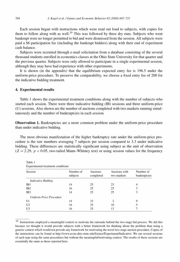
Table 1 shows the experimental treatment conditions along with the number of subjects whostarted each session. There were three indicative bidding (IB) sessions and three uniform-price(U) sessions. Also shown are the number of auctions completed with two markets running simul-taneously and the number of bankruptcies in each session.
Observation 1. Bankruptcies are a more common problem under the uniform-price procedurethan under indicative bidding.
The most obvious manifestation of the higher bankruptcy rate under the uniform-price pro-cedure is the raw numbers averaging 7 subjects per session compared to 3.3 under indicativebidding. These differences are statistically significant using subject as the unit of observation(Z = 2.29, p < 0.05, two-tailed Mann–Whitney test) or using session values for the frequency
Table 1Experimental treatment conditions
Session Number ofsubjects
Auctionscompleted
Auctions withtwo markets
Number ofbankruptcies
Indicative BiddingIB1 14 25 23 4IB2 16 25 25 3IB3 14 25 25 3
Uniform-Price ProcedureUl 14 23 2 9U2 16 25 10 5U3 16 25 13 7
19 Instructions employed a meaningful context to motivate the rationale behind the two-stage bid process. We did thisbecause we thought it would provide subjects with a better framework for thinking about the problem than using ageneric context which would not provide any framework for motivating the novel two-stage auction procedure. Copies ofthe instructions can be found at http://www.econ.ohio-state.edu/lixinye/Experiment/Indicative. We ran several sessionsof each type using the same procedures but without the meaningful/motivating context. The results of these sessions areessentially the same as those reported here.
J. Kagel et al. / Games and Economic Behavior 62 (2008) 697–721 705
with which subjects went bankrupt (p < 0.10, two-tailed Mann–Whitney test). This also showsup in terms of the number of auctions in which two markets operated simultaneously, whichlasted for all 25 auctions under indicative biding in almost all cases, but for a maximum of 13auctions with the uniform-price procedure. Given that most of the bankruptcies occurred early inthe uniform-price case, and in keeping with common practice in the experimental literature, inwhat follows we will distinguish between early auctions (1–12) where subjects are still learningand later auctions (13–25) where the most inept bidders have been eliminated and remainingbidders are well along in the learning process.
4.1. First-stage bids and entry efficiency
The primary motivation for examining alternatives to indicative bidding is that the latter can-not guarantee, in theory, efficient entry into the second stage, whereas the alternative biddingprocedure can. Thus, the question to be answered in this section is how actual efficiency com-pares across auction institutions.
Table 2 reports entry efficiency under both auction institutions. Three efficiency measures arereported: the first is the frequency with which the bidders with the highest and second higheststage-one values (X1;6 and X2;6) entered the second stage. The second is the frequency withwhich the bidders with the highest or the second highest stage-one values (X1;6 or X2;6) enteredthe second stage. These frequency measures are “rough” since they account only for who getsinto the second stage, but not for the loss of efficiency associated with lower valued biddersgetting into the second stage. The third efficiency measure calculates the ratio of the sum of thefirst-stage values for those actually entering the second stage divided by the sum of the highesttwo first-stage values. This is the conventional efficiency measure employed in the experimentalauction literature (referred to as the ratio efficiency in the table).
Table 2Entry efficiency
Percentage of X1,6 &X2,6 enter stage two
Percentage of X1,6 orX2,6 enter stage two
Ratio efficiency
Session: 1–12 13–25 All 1–12 13–25 All 1–12 13–25 All
Indicative BiddingIB1 16.7 25.0 20.8 95.8 95.8 95.8 87.8 90.2 89.0
(7.8) (9.0) (5.9) (4.2) (4.2) (2.9) (2.2) (1.9) (1.4)
IB2 41.7 50.0 46.0 91.7 100 96.0 91.8 95.5 93.8(10.3) (10.0) (7.1) (5.8) (0.0) (2.8) (2.2) (1.2) (1.2)
IB3 23.5 23.8 23.7 70.6 85.7 78.9 85.7 89.9 88.0(10.6) (9.5) (7.0) (11.4) (7.8) (6.7) (3.1) (1.8) (1.7)
IB 29.2 31.6 30.4 86.1 94.7 90.5 88.6 91.6 90.2Average (5.4) (5.4) (3.8) (4.1) (2.6) (2.4) (1.4) (1.0) (0.8)
Uniform ProcedureU1 14.3 36.4 24.0 85.7 100 92.0 89.7 93.5 91.4
(9.7) (15.2) (8.7) (9.7) (0) (5.5) (2.3) (2.0) (1.6)
U2 31.8 23.1 28.6 90.9 84.6 88.6 92.4 93.8 92.9(10.2) (12.2) (7.7) (6.3) (10.4) (5.5) (2.3) (2.1) (1.6)
U3 11.1 15.4 12.9 77.8 76.9 77.4 84.2 85.0 84.5(7.6) (10.4) (6.1) (10.1) (12.2) (7.6) (3.0) (3.9) (2.4)
U 19.6 24.3 21.5 85.7 86.5 86.0 88.8 90.6 89.5Average (5.4) (7.2) (4.3) (4.7) (5.7) (3.6) (1.5) (1.8) (1.1)
706 J. Kagel et al. / Games and Economic Behavior 62 (2008) 697–721
With the exception of the first two measures in the second uniform-price session (U2), allof the efficiency measures in all sessions are increasing with experience between auctions 1–12and 13–25. And even in this exceptional case the conventional ratio efficiency measure increasesbetween auctions 1–12 and 13–25. Furthermore, although the average frequency with whichbidders with the highest and second-highest first-stage values entered stage two is relativelylow in both treatments (30.4 and 21.5% overall for the indicative bidding and uniform-pricetreatments respectively), they are significantly higher than one would expect if stage-one bidswere strictly random (6.7%). Most importantly, looking at overall averages between treatments,with the exception of the standard ratio efficiency measure for auctions 1–12, efficiency is higherunder indicative bidding than under the uniform-price procedure. These differences are, however,quite small so that it comes as no surprise that for all three efficiency measures we are unable toreject a null hypothesis of no difference in efficiency between treatments at anything approachingconventional significance levels (using Mann–Whitney tests with auction outcomes as the unit ofobservation).
Observation 2. Efficiency is generally improving with experience and clearly beats random bid-ding under both procedures. Overall efficiency measures tend to be a bit higher under indicativebidding than the alternative procedure, but none of the differences approach statistical signif-icance at conventional levels. Thus, we conclude that indicative bidding does as well as thealternative bidding procedure in generating entry efficiency.
Table 3 checks for the monotonicity of the first-stage bid functions by looking at Spearmanrank order correlations between first-stage bids and values averaged by auction period from thetwo auction institutions.20 Looking at auction periods 1–12, rank order correlations are higherunder indicative bidding than the uniform-price procedure in 10 of the 12 periods, which isstatistically significant at the 10% level using a two-tailed sign test. However, in periods 13–25average rank order correlations by auction period are higher as often under indicative bidding asunder the uniform-price institution (7 out of 13 periods). Thus, in terms of the monotonicity offirst-stage bidding, indicative bidding does better than the uniform-price scheme early on in thebidding process, with the two essentially tied after that.21
Observation 3. Spearman rank order correlations are used to check the consistency with whichstage-one bids increase with stage-one values. Average Spearman rank order correlations byauction period are consistently higher early on under indicative bidding than under the uniform-price procedure, but are essentially the same after that.
The uniform-price bidding procedure produced entry fees that were significantly higher thanpredicted: The average realized entry fee (with the standard error of the mean in parentheses)
20 That is, for each auction market we calculate the relevant correlation coefficient first. We then average across marketsfor a given auction period. Thus, for example, the data reported for period 4 under IB represents the average of six auctionmarkets (2 for each session times 3 sessions).21 Under both procedures, we occasionally got negative rank order correlations in a particular auction. These are usuallyswamped by positive correlations in other auctions for the same auction period. This did not happen in period 25 in theuniform-price case where there were only two auctions—one with a negative rank order correlation of −0.580 and theother with a positive rank order correlation of 0.314. Larger negative rank order correlations than this can be found inother auctions.
J. Kagel et al. / Games and Economic Behavior 62 (2008) 697–721 707
Table 3Correlation coefficients for first-stage bids relative to values, by perioda
Period Spearman rank order correlations
Indicative Uniform
1 0.539 0.3442 0.373 0.3493 0.500 0.2994 0.292 0.1945 0.300 0.3836 0.299 0.2377 0.432 0.3378 0.521 0.4439 0.342 0.682
10 0.788 0.53911 0.491 0.44812 0.664 0.34513 0.373 0.18014 0.493 0.79015 0.297 0.68616 0.486 0.28617 0.390 0.37218 0.630 0.67019 0.283 0.54020 0.403 0.46721 0.522 0.53722 0.775 0.32423 0.606 0.04824 0.720 0.60025 0.269 −0.133
a Averaged across auction markets in each period.
is 426.7 (26.8) over all rounds, and 280.8 (24.2) over the last 13 rounds, versus predicted entryfees of 196.5. These much larger than predicted entry fees contributed substantially to the highbankruptcy rates under the uniform-price procedure.
4.2. Individual subject stage-one bid patterns
The efficiency data reported above relates to market measures of entry efficiency. The dataleaves unanswered the question as to individual subject bid patterns that give rise to these effi-ciency measures. That is, what are the underlying rules of thumb bidders use to produce betterthan random entry into stage-two under indicative bidding? What are the individual subject bidpatterns that result in less than the predicted full efficiency under the uniform-price procedure?
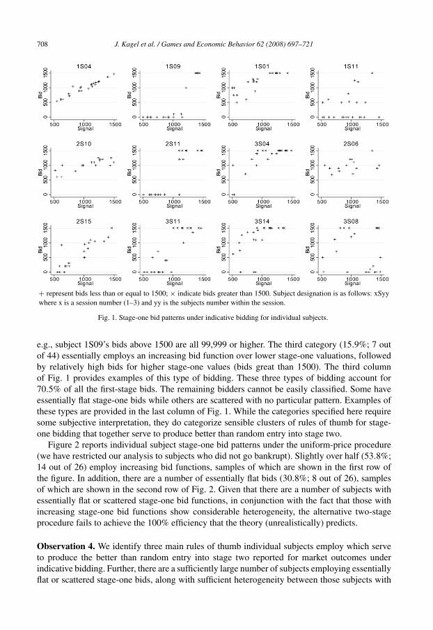
Figure 1 reports individual subject bid patterns under indicative bidding. We have identifiedthree primary rules of thumb that subjects employed. First, a number of subjects (31.8%; 14 outof 44) have essentially increasing bid functions—the higher their first-stage signals, the highertheir first-stage bids, with all bids being less than or equal to 1500. The first column of Fig. 1provides three examples of this type of bidding. The second category (22.7%; 10 out of 44)essentially employs a step function, with low bids for low stage-one valuations and substantiallyhigher bids for higher stage-one valuations. The second column of Fig. 1 provides three examplesof this type of bidding. Note that in these cases bids above 1500 are usually well above 1500;
708 J. Kagel et al. / Games and Economic Behavior 62 (2008) 697–721
+ represent bids less than or equal to 1500; × indicate bids greater than 1500. Subject designation is as follows: xSyywhere x is a session number (1–3) and yy is the subjects number within the session.
Fig. 1. Stage-one bid patterns under indicative bidding for individual subjects.
e.g., subject 1S09’s bids above 1500 are all 99,999 or higher. The third category (15.9%; 7 outof 44) essentially employs an increasing bid function over lower stage-one valuations, followedby relatively high bids for higher stage-one values (bids great than 1500). The third columnof Fig. 1 provides examples of this type of bidding. These three types of bidding account for70.5% of all the first-stage bids. The remaining bidders cannot be easily classified. Some haveessentially flat stage-one bids while others are scattered with no particular pattern. Examples ofthese types are provided in the last column of Fig. 1. While the categories specified here requiresome subjective interpretation, they do categorize sensible clusters of rules of thumb for stage-one bidding that together serve to produce better than random entry into stage two.
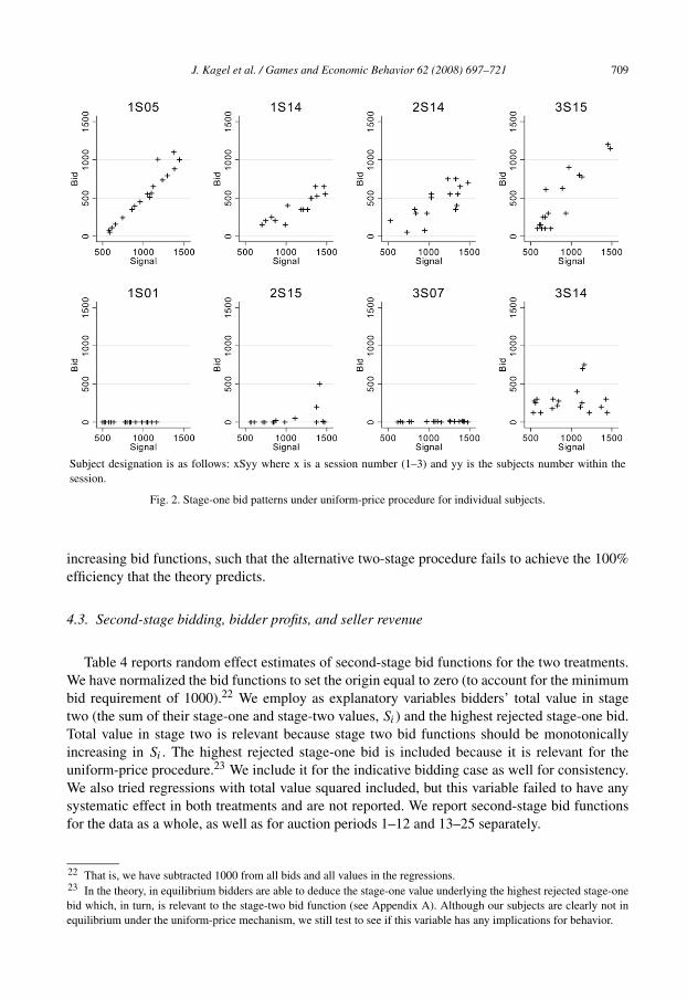
Figure 2 reports individual subject stage-one bid patterns under the uniform-price procedure(we have restricted our analysis to subjects who did not go bankrupt). Slightly over half (53.8%;14 out of 26) employ increasing bid functions, samples of which are shown in the first row ofthe figure. In addition, there are a number of essentially flat bids (30.8%; 8 out of 26), samplesof which are shown in the second row of Fig. 2. Given that there are a number of subjects withessentially flat or scattered stage-one bid functions, in conjunction with the fact that those withincreasing stage-one bid functions show considerable heterogeneity, the alternative two-stageprocedure fails to achieve the 100% efficiency that the theory (unrealistically) predicts.
Observation 4. We identify three main rules of thumb individual subjects employ which serveto produce the better than random entry into stage two reported for market outcomes underindicative bidding. Further, there are a sufficiently large number of subjects employing essentiallyflat or scattered stage-one bids, along with sufficient heterogeneity between those subjects with
J. Kagel et al. / Games and Economic Behavior 62 (2008) 697–721 709
Subject designation is as follows: xSyy where x is a session number (1–3) and yy is the subjects number within thesession.
Fig. 2. Stage-one bid patterns under uniform-price procedure for individual subjects.
increasing bid functions, such that the alternative two-stage procedure fails to achieve the 100%efficiency that the theory predicts.
4.3. Second-stage bidding, bidder profits, and seller revenue
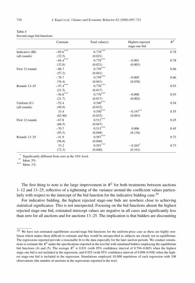
Table 4 reports random effect estimates of second-stage bid functions for the two treatments.We have normalized the bid functions to set the origin equal to zero (to account for the minimumbid requirement of 1000).22 We employ as explanatory variables bidders’ total value in stagetwo (the sum of their stage-one and stage-two values, Si ) and the highest rejected stage-one bid.Total value in stage two is relevant because stage two bid functions should be monotonicallyincreasing in Si. The highest rejected stage-one bid is included because it is relevant for theuniform-price procedure.23 We include it for the indicative bidding case as well for consistency.We also tried regressions with total value squared included, but this variable failed to have anysystematic effect in both treatments and are not reported. We report second-stage bid functionsfor the data as a whole, as well as for auction periods 1–12 and 13–25 separately.
22 That is, we have subtracted 1000 from all bids and all values in the regressions.23 In the theory, in equilibrium bidders are able to deduce the stage-one value underlying the highest rejected stage-onebid which, in turn, is relevant to the stage-two bid function (see Appendix A). Although our subjects are clearly not inequilibrium under the uniform-price mechanism, we still test to see if this variable has any implications for behavior.
710 J. Kagel et al. / Games and Economic Behavior 62 (2008) 697–721
Table 4Second-stage bid functions
Constant Total value(s) Highest rejectedstage-one bid
R2
Indicative (IB) −85.6*** 0.778*** 0.78(all rounds) (32.5) (0.021)
−84.4*** 0.778*** −0.001 0.78(32.8) (0.021) (0.003)
First 12 rounds −86.7 0.759*** 0.66(57.2) (0.041)
−79.7 0.759*** −0.005 0.66(76.4) (0.041) (0.038)
Rounds 13–25 −57.4*** 0.776*** 0.93(21.5) (0.017)
−56.8*** 0.776*** −0.000 0.93(21.7) (0.017) (0.002)
Uniform (U) −52.4 0.540*** 0.54(all rounds) (49.9) (0.032)
33.4 0.550*** −0.197** 0.55(82.90) (0.032) (0.093)
First 12 rounds −67.8 0.513*** 0.45(66.5) (0.047)
−70.7 0.513*** 0.006 0.45(95.5) (0.048) (0.136)
Rounds 13–25 −41.9 0.587*** 0.72(56.8) (0.040)
33.2 0.591*** −0.265* 0.73(72.3) (0.040) (0.161)
* Significantly different from zero at the 10% level.** Idem, 5%.
*** Idem, 1%.
The first thing to note is the large improvement in R2 for both treatments between auctions1–12 and 13–25, reflective of a tightening of the variance around the coefficient values particu-larly with respect to the intercept of the bid function for the indicative bidding case.24
For indicative bidding, the highest rejected stage-one bids are nowhere close to achievingstatistical significance. This is not unexpected. Focusing on the bid functions absent the highestrejected stage-one bid, estimated intercept values are negative in all cases and significantly lessthan zero for all auctions and for auctions 13–25. The implication is that bidders are discounting
24 We have not estimated equilibrium second-stage bid functions for the uniform-price case as these are highly non-linear which makes them difficult to estimate and they would be misspecified as subjects are clearly not in equilibrium.The regressions reported provide a reasonable fit to the data especially for the later auction periods. We conduct simula-tions to estimate the R2 under the specifications reported in the text but with simulated bidders employing the equilibriumbid functions (4) and (5). The average R2 is 0.831 (with 95% confidence interval of 0.794–0.865) when the higheststage-one bid is not included in the regression, and 0.925 (with 95% confidence interval of 0.898–0.948) when the high-est stage-one bid is included in the regression. Simulations employed 10,000 repetitions of each regression with 108observations (the number of auctions in the regressions reported in the text).
J. Kagel et al. / Games and Economic Behavior 62 (2008) 697–721 711
their bids relative to their values somewhat less at higher values. This may reflect an attempt bybidders with low total values to recover some portion of their stage-one entry fee.25
For the uniform-price case the highest rejected stage-one bid constitutes the common entryfee stage-two bidders must pay. Without the highest rejected stage-one bid as a right-hand sidevariable, the intercepts of the estimated bid functions for the uniform-price case are not signif-icantly different from zero. Further, for both specifications the slopes of the bid functions areflatter, much flatter than with indicative bidding. However, with the highest rejected stage-onebid variable the coefficient is negative in sign and statistically significant for the pooled dataacross all treatments, and for auctions 13–25 where the coefficient value is negative and is sta-tistically significant at the 10% level in a two-tailed test.26 The negative sign for the entry feevariable has minimal impact on average second-stage bids since with its inclusion the interceptof the bid function becomes positive and the coefficient for total value increases a bit.27
The theory implies that the highest rejected stage-one bid will be positive in sign at lowerstage-one values (Si � 2000) and can possibly (but not necessarily) be negative in sign forSi > 2000. But this is true only in equilibrium, and we already know from the efficiencydata that bidders are relatively far from equilibrium. As such we look elsewhere for a pos-sible explanation for the statistical significance of the entry fee variable in the uniform-pricecase. One possibility is suggested by results from coordination games (games with multi-ple Pareto ranked equilibria) in which the imposition of an entry fee affects which equi-libria subjects will coordinate on, with higher entry fees reliably inducing Pareto improv-ing (i.e., more profitable) equilibria in the coordination game itself (Van Huyck et al., 1993;Cachon and Camerer, 1996). Cachon and Camerer’s experiment indicates quite clearly that sub-jects in these coordination games take account of the entry fees, employing a “loss-avoidance”selection principle in making their choices in the coordination game, and expecting others to dothe same. Applying this principle here, higher entry fees in the uniform-price auctions inducebidders to lower their bids in the second stage in an effort to avoid losses, with some confidencethat their second-stage rival will do the same, as the entry fees are common and publicly known.
Observation 5. Second stage bid functions are monotonically increasing in total value as theyshould be, with slopes well below 1.0 in both treatments. The highest rejected stage-one bid isstatistically significant in the uniform-price procedures, suggesting that bidders are attempting toavoid possible losses associated with higher entry fees in this case.
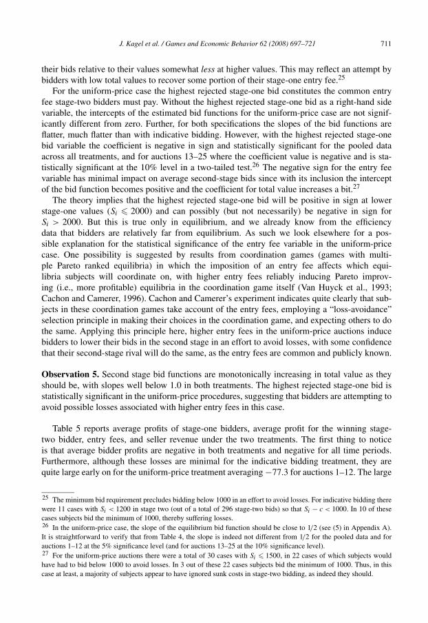
Table 5 reports average profits of stage-one bidders, average profit for the winning stage-two bidder, entry fees, and seller revenue under the two treatments. The first thing to noticeis that average bidder profits are negative in both treatments and negative for all time periods.Furthermore, although these losses are minimal for the indicative bidding treatment, they arequite large early on for the uniform-price treatment averaging −77.3 for auctions 1–12. The large
25 The minimum bid requirement precludes bidding below 1000 in an effort to avoid losses. For indicative bidding therewere 11 cases with Si < 1200 in stage two (out of a total of 296 stage-two bids) so that Si − c < 1000. In 10 of thesecases subjects bid the minimum of 1000, thereby suffering losses.26 In the uniform-price case, the slope of the equilibrium bid function should be close to 1/2 (see (5) in Appendix A).It is straightforward to verify that from Table 4, the slope is indeed not different from 1/2 for the pooled data and forauctions 1–12 at the 5% significance level (and for auctions 13–25 at the 10% significance level).27 For the uniform-price auctions there were a total of 30 cases with Si � 1500, in 22 cases of which subjects wouldhave had to bid below 1000 to avoid losses. In 3 out of these 22 cases subjects bid the minimum of 1000. Thus, in thiscase at least, a majority of subjects appear to have ignored sunk costs in stage-two bidding, as indeed they should.
712 J. Kagel et al. / Games and Economic Behavior 62 (2008) 697–721
Table 5Bidder profits and seller revenue (standard errors in parenthesis)
Average profit ofstage-one bidders
Average winner’sprofit
Entry fees Seller revenue
Actual Predicted Actual Predicted Actual Predicted Actual Predicted
Indicative −6.65** NA 160.10** NA 200 200 2107.18 NA(all rounds) (2.61) (15.69) (30.59)
First 12 −7.59** 154.47** 2121.11(3.62) (21.72) (44.75)
Rounds 13–25 −5.76 165.43** 2093.99(3.78) (22.70) (42.09)
Uniform −47.44** 29.8 164.16** 375.0 426.7 196.5 2212.52 1992.0(all rounds) (10.37) (46.93) (26.8) (63.55)
First 12 −77.26** 80.85 528.5 2392.73(14.73) (69.88) (36.4) (86.56)
Rounds 13–25 −2.32 290.24** 280.8 1939.76(9.72) (46.08) (24.2) (71.98)
NA = not applicable.** Significantly different form zero at the 5% level.
losses in this last case are directly accounted for by the much higher than predicted entry feeswhich averaged 528.5 for auctions 1–12 as opposed to the 196.5 predicted. In both treatments,and in all time periods, the winner of the second-stage auction earned positive average profitsafter accounting for entry fees.
However, these profits were not enough to compensate for the fact that under the auction rulesboth stage-two bidders pay entry fees. These negative average profits account for the bankruptciesreported under both treatments. Furthermore, the much larger early losses under the uniform-price treatment account for the heavy early attrition under that treatment.
A closer look at the profit data shows that for the indicative bidding treatments, when bidderswith the highest or second-highest stage-one values got into stage two they earned positive av-erage profits, regardless of whether they won or not. In contrast, bidders getting into stage twowith lower stage-one values earned relatively large negative profits, in large measure becausethey were much less likely to win the stage-two auction, while still paying the 200 entry fee.(Bidders with the highest or second-highest stage-one value won in stage two about twice asoften as those with lower stage-one values: 61.5% of the time versus 32.5%.)
For the uniform-price auctions the high entry fees in auctions 1–12 make for negative averageprofits even for those bidders with the highest or second-highest stage-one values who madeit into stage two. Not surprisingly, things were even worse, on average, for those who got intostage-two with lower stage-one values. For auctions 13–25, with their lower stage-one entry fees,bidders with the highest or second-highest stage-one value who made it into stage two earnedpositive average profits regardless of whether they won the stage-two auction or not. Bidders withlower stage-one values continued to earn negative average profits, largely as a result of winningmuch less often after making it into stage two (30.3% of the time versus 65.9%).
That these inefficient entries largely account for the negative average profits under both auc-tion institutions is confirmed through simulations in which we use the estimated stage-two bidfunction to determine average profits conditional on only the highest and second-highest stage-one value holders entering stage two. With the exception of auctions 1–12 in the uniform-priceauctions, the simulations show modest positive profits averaged over all bidders due to the
J. Kagel et al. / Games and Economic Behavior 62 (2008) 697–721 713
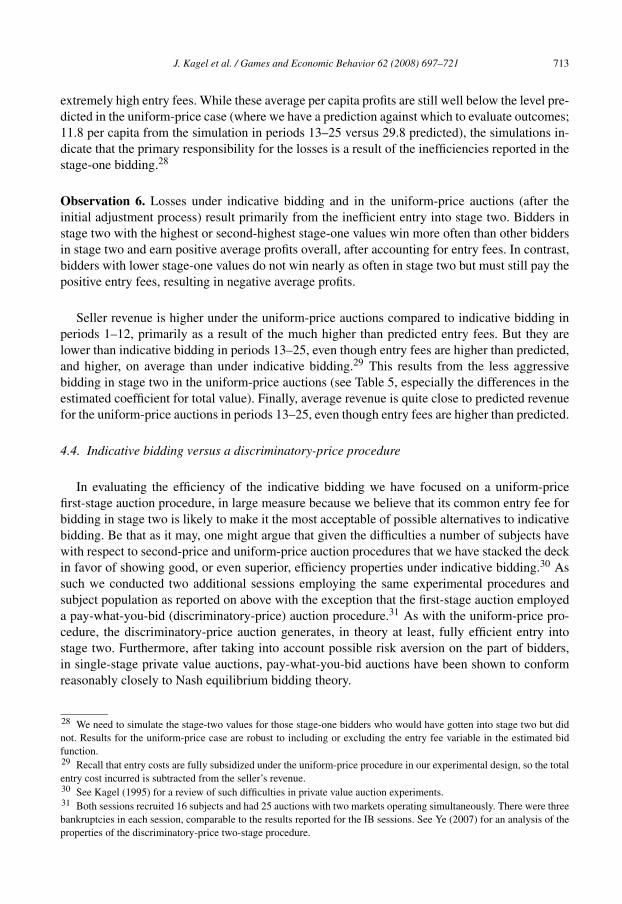
extremely high entry fees. While these average per capita profits are still well below the level pre-dicted in the uniform-price case (where we have a prediction against which to evaluate outcomes;11.8 per capita from the simulation in periods 13–25 versus 29.8 predicted), the simulations in-dicate that the primary responsibility for the losses is a result of the inefficiencies reported in thestage-one bidding.28
Observation 6. Losses under indicative bidding and in the uniform-price auctions (after theinitial adjustment process) result primarily from the inefficient entry into stage two. Bidders instage two with the highest or second-highest stage-one values win more often than other biddersin stage two and earn positive average profits overall, after accounting for entry fees. In contrast,bidders with lower stage-one values do not win nearly as often in stage two but must still pay thepositive entry fees, resulting in negative average profits.
Seller revenue is higher under the uniform-price auctions compared to indicative bidding inperiods 1–12, primarily as a result of the much higher than predicted entry fees. But they arelower than indicative bidding in periods 13–25, even though entry fees are higher than predicted,and higher, on average than under indicative bidding.29 This results from the less aggressivebidding in stage two in the uniform-price auctions (see Table 5, especially the differences in theestimated coefficient for total value). Finally, average revenue is quite close to predicted revenuefor the uniform-price auctions in periods 13–25, even though entry fees are higher than predicted.
4.4. Indicative bidding versus a discriminatory-price procedure
In evaluating the efficiency of the indicative bidding we have focused on a uniform-pricefirst-stage auction procedure, in large measure because we believe that its common entry fee forbidding in stage two is likely to make it the most acceptable of possible alternatives to indicativebidding. Be that as it may, one might argue that given the difficulties a number of subjects havewith respect to second-price and uniform-price auction procedures that we have stacked the deckin favor of showing good, or even superior, efficiency properties under indicative bidding.30 Assuch we conducted two additional sessions employing the same experimental procedures andsubject population as reported on above with the exception that the first-stage auction employeda pay-what-you-bid (discriminatory-price) auction procedure.31 As with the uniform-price pro-cedure, the discriminatory-price auction generates, in theory at least, fully efficient entry intostage two. Furthermore, after taking into account possible risk aversion on the part of bidders,in single-stage private value auctions, pay-what-you-bid auctions have been shown to conformreasonably closely to Nash equilibrium bidding theory.
28 We need to simulate the stage-two values for those stage-one bidders who would have gotten into stage two but didnot. Results for the uniform-price case are robust to including or excluding the entry fee variable in the estimated bidfunction.29 Recall that entry costs are fully subsidized under the uniform-price procedure in our experimental design, so the totalentry cost incurred is subtracted from the seller’s revenue.30 See Kagel (1995) for a review of such difficulties in private value auction experiments.31 Both sessions recruited 16 subjects and had 25 auctions with two markets operating simultaneously. There were threebankruptcies in each session, comparable to the results reported for the IB sessions. See Ye (2007) for an analysis of theproperties of the discriminatory-price two-stage procedure.
714 J. Kagel et al. / Games and Economic Behavior 62 (2008) 697–721
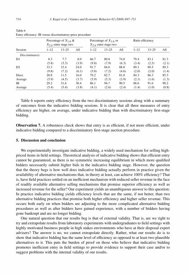
Table 6Entry efficiency: IB versus discriminatory-price procedure
Percentage of X1;6 &X2;6 enter stage two
Percentage of X1;6 orX2;6 enter stage two
Ratio efficiency
Session: 1–12 13–25 All 1–12 13–25 All 1–12 13–25 All
DiscriminatoryD1 8.3 7.7 8.0 66.7 80.8 74.0 79.4 83.1 81.3
(5.8) (5.3) (3.9) (9.8) (7.9) (6.3) (3.4) (2.5) (2.1)
D2 33.3 15.4 24.0 91.7 84.6 88.0 89.1 89.5 89.3(9.8) (7.2) (6.1) (5.8) (7.2) (4.6) (2.0) (2.0) (1.4)
Discr. 20.8 11.5 16.0 79.2 82.7 81.0 84.3 86.3 85.3Average (5.9) (4.5) (3.7) (5.9) (5.3) (3.9) (2.1) (1.6) (1.3)
IB 29.2 31.6 30.4 86.1 94.7 90.5 88.6 91.6 90.2Average (5.4) (5.4) (3.8) (4.1) (2.6) (2.4) (1.4) (1.0) (0.8)
Table 6 reports entry efficiency from the two discriminatory sessions along with a summaryof outcomes from the indicative bidding sessions. It is clear that all three measures of entryefficiency are higher, on average, under indicative bidding than with discriminatory first-stagebidding.
Observation 7. A robustness check shows that entry is as efficient, if not more efficient, underindicative bidding compared to a discriminatory first-stage auction procedure.
5. Discussion and conclusion
We experimentally investigate indicative bidding, a widely used mechanism for selling high-priced items in field settings. Theoretical analysis of indicative bidding shows that efficient entrycannot be guaranteed, as there is no symmetric increasing equilibrium in which more qualifiedbidders necessarily submit higher bids in the indicative bidding stage. However, the questionthat the theory begs is how well does indicative bidding actually perform in practice given theavailability of alternative mechanisms that, in theory at least, can achieve 100% efficiency? Thatis, have field practices settled on an inefficient mechanism with reduced seller revenue in the faceof readily available alternative selling mechanisms that promise superior efficiency as well asincreased revenue for the seller? Our experiment yields an unambiguous answer to this question:In practice indicative bidding yields efficiency levels that are the same, if not better, than twoalternative bidding practices that promise both higher efficiency and higher seller revenue. Thisoccurs both early on when bidders are adjusting to the more complicated alternative biddingprocedures as well as after bidders have gained experience, with a number of bidders havinggone bankrupt and are no longer bidding.
One natural question that our results beg is that of external validity. That is, are we right totry and extrapolate results from laboratory experiments with undergraduates to field settings withhighly motivated business people in high stakes environments who have at their disposal expertadvisers? The answer is no, we cannot extrapolate directly. Rather, what our results do is toshow that indicative bidding has the same level of efficiency as opposed to at least two plausiblealternatives to it. This puts the burden of proof on those who believe that indicative biddingpromotes inefficient entry in field settings to provide evidence to support their case and/or tosuggest problems with the internal validity of our results.
J. Kagel et al. / Games and Economic Behavior 62 (2008) 697–721 715
In extrapolating results from the laboratory to field settings one also needs to look at the mech-anism underlying the laboratory results. Is the same, or a similar, mechanism likely to be presentin field settings as well? We believe the answer is yes in this case. The mechanism promotingthe relatively high efficiency levels observed in our experiment is the one in which bidders withhigher stage-one values can anticipate positive average profits, while those with lower stage-onevalues earned negative average profits. A similar mechanism for promoting respectable entryefficiency can be expected to operate in field settings since, in addition to possibly earning neg-ative profits as a result of unwise entry, bidders in field settings have alternative income earningopportunities to pursue with their limited resources which should discourage bidders with lowstage-one values from bidding very aggressively.
Our results highlight a potential trade-off between different types of mechanisms: Those withrelatively simple rules but less clear, or weaker, equilibrium outcomes, and those with relativelymore complicated rules but clear underlying equilibrium outcomes. While game theorists areproperly concerned with the existence and uniqueness of an equilibrium, selecting a mechanismbased only on its underlying equilibrium properties can be misleading. For a mechanism to workin practice, simplicity and transparency are as important, if not more so, than equilibrium con-siderations.
What precisely underlies the greater simplicity of indicative bidding over the alternative bid-ding mechanisms employed here? To answer this we first introduce a definition for complexityagainst which to compare the different mechanisms. A quick look at the literature shows a largenumber of definitions for measuring complexity.32 One definition that seems appropriate to oursituation is: “The difficulty of making correct predictions about its environment (measured byits error rate) for an agent using the best model it can infer from the information available toit given its computational resources” (Edmonds, 1997). Applying this definition to the presentstudy, the endogenously determined entry fee under the uniform-price procedure would qual-ify as more complex, due to its inherent variability, compared to the exogenously determinedfixed fee under indicative bidding.33 Under the discriminatory-price procedure bidders deter-mine the entry fee with their first-stage bids. However, these first-stage bids are binding, whichrequires a rather complicated backward induction calculation to determine the equilibrium first-stage bid. In contrast, under indicative bidding the entry fee/cost for each entrant is fixed andknown with certainty. Although stage-one bids remain non-trivial under indicative bidding, asthe existence of a sensible equilibrium is an open question, we believe that the fact that thestage-one bidding does not directly impact the entry fee simplifies the stage-one bidding strat-egy.
Our analysis has focused on efficiency comparison between indicative bidding and theuniform-price procedure, as this would appear to be the relevant and fully efficient auction bench-mark for situations where indicative bidding is applied in practice. As noted, a uniform-priceprocedure would seem to be “fairer” than a discriminatory-price procedure, with the fairness is-sue becoming more important the higher and more disparate the first-stage bids. But this begs thequestion as to why we do not compare indicative bidding to a benchmark based on a single-stage
32 Just search under “measuring complexity” on the Internet.33 This greater complexity still remains even if a second-price auction is employed in stage two, as entry fees are stillendogenously determined, hence inherently variable.
716 J. Kagel et al. / Games and Economic Behavior 62 (2008) 697–721
procedure where bidders simultaneously and independently make their entry decisions.34 Theanswer is that for the type of assets in question, this is not a practical procedure as there may beconstraints on how many bidders can be admitted to the due diligence process. For example, inthe electrical generating asset sales, the seller may need to consider how many data rooms can beprovided (a capacity constraint), or there may be security concerns about information leakage iftoo many or the wrong bidders are admitted to the due diligence process. The two-stage auctionprocedure (indicative bidding or the alternative mechanisms considered in our paper) solves thisproblem by selecting a targeted number of bidders for the final auction.
Our results provide a possible explanation for why indicative bidding is so commonly used,despite the lack of a clear equilibrium solution. The mechanism design problem in auction set-tings with costly entry is not easy, as the optimal auction in general should not include all thebidders in the final sale. But how to pre-select the most qualified bidders is not trivial. Theoret-ical analysis reveals that non-binding bidding in the first stage results in the non-existence of asymmetric increasing equilibrium. Therefore, to restore incentive compatibility, it is necessaryto make the first-stage bids binding. Bidding for entry rights with entry fee payments is a naturalway to solve the problem. No doubt the analysis here has not exhausted the possible alternativebid procedures promising full efficiency, but we conjecture that the rules of the two alterna-tive institutions employed here are among the simplest within the class of selling mechanismsthat require binding first-round bidding. Thus, if these alternative bid procedures fail to exhibitadvantages over indicative bidding, there is good reason to appreciate indicative bidding. It iscertainly not perfect, but the present results indicate that it works well enough relative to viableand somewhat more complicated alternatives.
Acknowledgments
We thank Susan Rose, Kirill Chernomaz, and Jose Mustre for their excellent research as-sistance. Kagel’s research was partially supported by National Science Foundation Grants No.0136925 and 0136928. Ye’s research was supported by a seed grant from the Ohio State Univer-sity. Any opinions, findings, and conclusions or recommendations in this material are those of theauthors and do not necessarily reflect the views of the National Science Foundation or the OhioState University. We have benefited from comments of seminar participants at the Ohio StateUniversity, the Winter Econometric Society Meetings (San Diego), the Conference on Auctionsat University of Iowa, and especially the comments of Dan Levin, James Peck, Ilya Segal, andan anonymous referee. The usual caveat applies.
Appendix A. Equilibrium analysis under the uniform-price procedure
In this appendix we will derive the equilibrium bidding function in the uniform-price proce-dure. In what follows we assume that X’s are drawn from [L,H ] uniformly, and Y takes valueeither H (with probability p) or L (with probability 1 − p). We define D = H − L to be thespread between the first-stage value upper bound and lower bound. In our experimental design,L = 500, H = 1500 (the value spread D = 1000), and p = 1/2.
34 More specifically, in the single-stage benchmark the bidders make entry decisions simultaneously and independentlybased on their stage-one signals. Once they decide to enter, each bidder incurs an entry cost c and learns her stage-twosignal. Finally, the entrant bidders bid for the asset in a standard sealed bid auction.
J. Kagel et al. / Games and Economic Behavior 62 (2008) 697–721 717
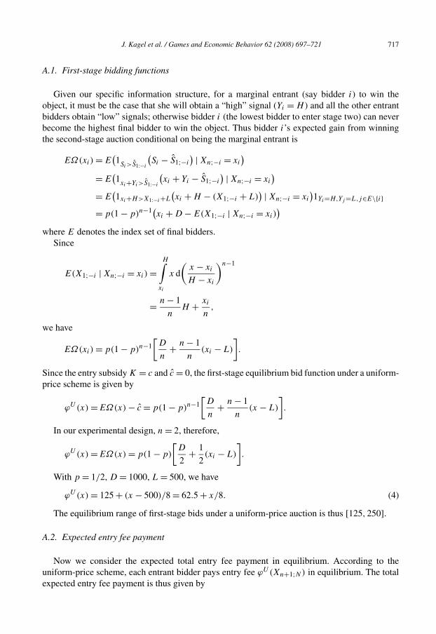
A.1. First-stage bidding functions
Given our specific information structure, for a marginal entrant (say bidder i) to win theobject, it must be the case that she will obtain a “high” signal (Yi = H ) and all the other entrantbidders obtain “low” signals; otherwise bidder i (the lowest bidder to enter stage two) can neverbecome the highest final bidder to win the object. Thus bidder i’s expected gain from winningthe second-stage auction conditional on being the marginal entrant is
EΩ(xi) = E(1Si>S1:−i
(Si − S1;−i
) | Xn;−i = xi
)= E
(1xi+Yi>S1:−i
(xi + Yi − S1;−i
) | Xn;−i = xi
)= E
(1xi+H>X1:−i+L
(xi + H − (X1;−i + L)
) | Xn;−i = xi
)1Yi=H,Yj =L,j∈E\{i}
= p(1 − p)n−1(xi + D − E(X1;−i | Xn;−i = xi))
where E denotes the index set of final bidders.Since
E(X1;−i | Xn;−i = xi) =H∫
xi
x d
(x − xi
H − xi
)n−1
= n − 1
nH + xi
n,
we have
EΩ(xi) = p(1 − p)n−1[D
n+ n − 1
n(xi − L)
].
Since the entry subsidy K = c and c = 0, the first-stage equilibrium bid function under a uniform-price scheme is given by
ϕU(x) = EΩ(x) − c = p(1 − p)n−1[D
n+ n − 1
n(x − L)
].
In our experimental design, n = 2, therefore,
ϕU(x) = EΩ(x) = p(1 − p)
[D
2+ 1
2(xi − L)
].
With p = 1/2, D = 1000, L = 500, we have
ϕU(x) = 125 + (x − 500)/8 = 62.5 + x/8. (4)
The equilibrium range of first-stage bids under a uniform-price auction is thus [125,250].
A.2. Expected entry fee payment
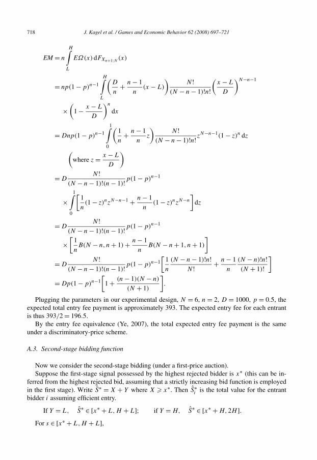
Now we consider the expected total entry fee payment in equilibrium. According to theuniform-price scheme, each entrant bidder pays entry fee ϕU(Xn+1;N) in equilibrium. The totalexpected entry fee payment is thus given by
718 J. Kagel et al. / Games and Economic Behavior 62 (2008) 697–721
EM = n
H∫L
EΩ(x)dFXn+1;N (x)
= np(1 − p)n−1
H∫L
(D
n+ n − 1
n(x − L)
)N !
(N − n − 1)!n!(
x − L
D
)N−n−1
×(
1 − x − L
D
)n
dx
= Dnp(1 − p)n−1
1∫0
(1
n+ n − 1
nz
)N !
(N − n − 1)!n!zN−n−1(1 − z)n dz
(where z = x − L
D
)
= DN !
(N − n − 1)!(n − 1)!p(1 − p)n−1
×1∫
0
[1
n(1 − z)nzN−n−1 + n − 1
n(1 − z)nzN−n
]dz
= DN !
(N − n − 1)!(n − 1)!p(1 − p)n−1
×[
1
nB(N − n,n + 1) + n − 1
nB(N − n + 1, n + 1)
]
= DN !
(N − n − 1)!(n − 1)!p(1 − p)n−1[
1
n
(N − n − 1)!n!N ! + n − 1
n
(N − n)!n!(N + 1)!
]
= Dp(1 − p)n−1[
1 + (n − 1)(N − n)
(N + 1)
].
Plugging the parameters in our experimental design, N = 6, n = 2, D = 1000, p = 0.5, theexpected total entry fee payment is approximately 393. The expected entry fee for each entrantis thus 393/2 = 196.5.
By the entry fee equivalence (Ye, 2007), the total expected entry fee payment is the sameunder a discriminatory-price scheme.
A.3. Second-stage bidding function
Now we consider the second-stage bidding (under a first-price auction).Suppose the first-stage signal possessed by the highest rejected bidder is x∗ (this can be in-
ferred from the highest rejected bid, assuming that a strictly increasing bid function is employedin the first stage). Write S∗ = X + Y where X � x∗. Then S∗
i is the total value for the entrantbidder i assuming efficient entry.
If Y = L, S∗ ∈ [x∗ + L,H + L]; if Y = H, S∗ ∈ [x∗ + H,2H ].For s ∈ [x∗ + L,H + L],
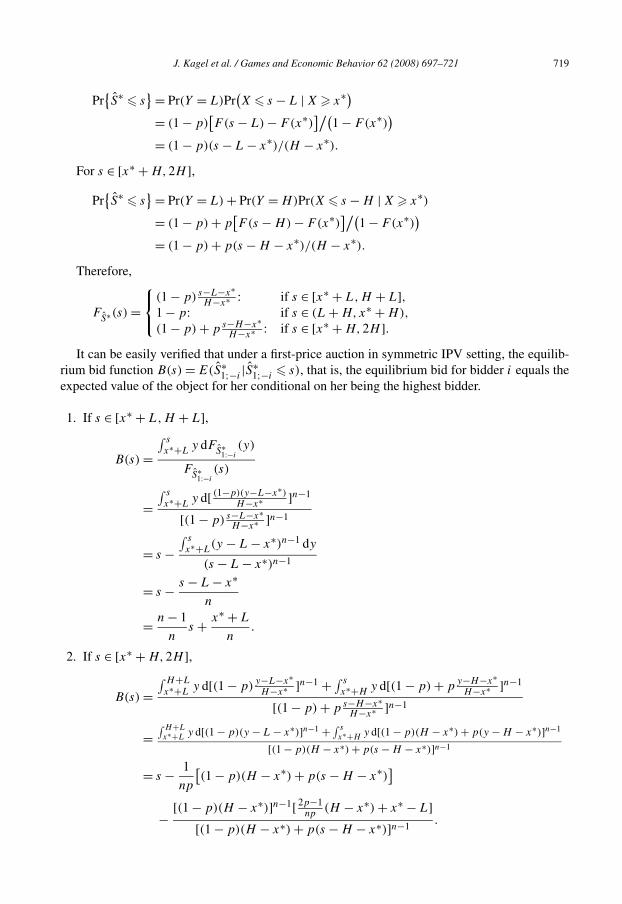
J. Kagel et al. / Games and Economic Behavior 62 (2008) 697–721 719
Pr{S∗ � s
} = Pr(Y = L)Pr(X � s − L | X � x∗)
= (1 − p)[F(s − L) − F(x∗)
]/(1 − F(x∗)
)= (1 − p)(s − L − x∗)/(H − x∗).
For s ∈ [x∗ + H,2H ],Pr
{S∗ � s
} = Pr(Y = L) + Pr(Y = H)Pr(X � s − H | X � x∗)= (1 − p) + p
[F(s − H) − F(x∗)
]/(1 − F(x∗)
)= (1 − p) + p(s − H − x∗)/(H − x∗).
Therefore,
FS∗(s) =
⎧⎨⎩
(1 − p)s−L−x∗H−x∗ : if s ∈ [x∗ + L,H + L],
1 − p: if s ∈ (L + H,x∗ + H),
(1 − p) + p s−H−x∗H−x∗ : if s ∈ [x∗ + H,2H ].
It can be easily verified that under a first-price auction in symmetric IPV setting, the equilib-rium bid function B(s) = E(S∗
1;−i|S∗
1;−i� s), that is, the equilibrium bid for bidder i equals the
expected value of the object for her conditional on her being the highest bidder.
1. If s ∈ [x∗ + L,H + L],
B(s) =∫ s
x∗+Ly dF
S∗1:−i
(y)
FS∗
1:−i(s)
=∫ s
x∗+Ly d[ (1−p)(y−L−x∗)
H−x∗ ]n−1
[(1 − p) s−L−x∗H−x∗ ]n−1
= s −∫ s
x∗+L(y − L − x∗)n−1 dy
(s − L − x∗)n−1
= s − s − L − x∗
n
= n − 1
ns + x∗ + L
n.
2. If s ∈ [x∗ + H,2H ],
B(s) =∫ H+L
x∗+Ly d[(1 − p)
y−L−x∗H−x∗ ]n−1 + ∫ s
x∗+Hy d[(1 − p) + p
y−H−x∗H−x∗ ]n−1
[(1 − p) + p s−H−x∗H−x∗ ]n−1
=∫ H+L
x∗+Ly d[(1 − p)(y − L − x∗)]n−1 + ∫ s
x∗+Hy d[(1 − p)(H − x∗) + p(y − H − x∗)]n−1
[(1 − p)(H − x∗) + p(s − H − x∗)]n−1
= s − 1
np
[(1 − p)(H − x∗) + p(s − H − x∗)
]
− [(1 − p)(H − x∗)]n−1[ 2p−1np
(H − x∗) + x∗ − L][(1 − p)(H − x∗) + p(s − H − x∗)]n−1
.
720 J. Kagel et al. / Games and Economic Behavior 62 (2008) 697–721
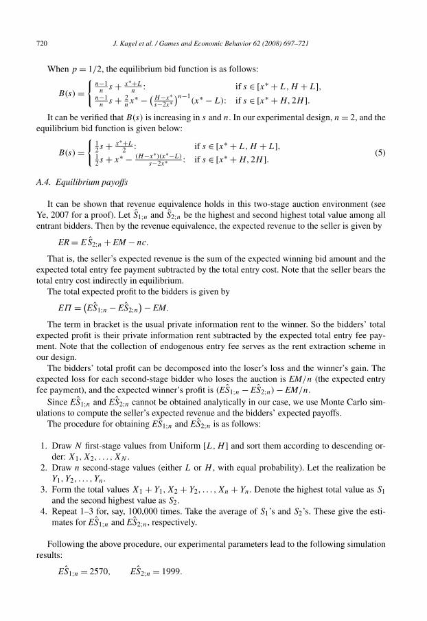
When p = 1/2, the equilibrium bid function is as follows:
B(s) ={
n−1n
s + x∗+Ln
: if s ∈ [x∗ + L,H + L],n−1n
s + 2nx∗ − (
H−x∗s−2x∗
)n−1(x∗ − L): if s ∈ [x∗ + H,2H ].
It can be verified that B(s) is increasing in s and n. In our experimental design, n = 2, and theequilibrium bid function is given below:
B(s) ={
12 s + x∗+L
2 : if s ∈ [x∗ + L,H + L],12 s + x∗ − (H−x∗)(x∗−L)
s−2x∗ : if s ∈ [x∗ + H,2H ]. (5)
A.4. Equilibrium payoffs
It can be shown that revenue equivalence holds in this two-stage auction environment (seeYe, 2007 for a proof). Let S1;n and S2;n be the highest and second highest total value among allentrant bidders. Then by the revenue equivalence, the expected revenue to the seller is given by
ER = ES2;n + EM − nc.
That is, the seller’s expected revenue is the sum of the expected winning bid amount and theexpected total entry fee payment subtracted by the total entry cost. Note that the seller bears thetotal entry cost indirectly in equilibrium.
The total expected profit to the bidders is given by
EΠ = (ES1;n − ES2;n
) − EM.
The term in bracket is the usual private information rent to the winner. So the bidders’ totalexpected profit is their private information rent subtracted by the expected total entry fee pay-ment. Note that the collection of endogenous entry fee serves as the rent extraction scheme inour design.
The bidders’ total profit can be decomposed into the loser’s loss and the winner’s gain. Theexpected loss for each second-stage bidder who loses the auction is EM/n (the expected entryfee payment), and the expected winner’s profit is (ES1;n − ES2;n) − EM/n.
Since ES1;n and ES2;n cannot be obtained analytically in our case, we use Monte Carlo sim-ulations to compute the seller’s expected revenue and the bidders’ expected payoffs.
The procedure for obtaining ES1;n and ES2;n is as follows:
1. Draw N first-stage values from Uniform [L,H ] and sort them according to descending or-der: X1,X2, . . . ,XN .
2. Draw n second-stage values (either L or H , with equal probability). Let the realization beY1, Y2, . . . , Yn.
3. Form the total values X1 + Y1,X2 + Y2, . . . ,Xn + Yn. Denote the highest total value as S1and the second highest value as S2.
4. Repeat 1–3 for, say, 100,000 times. Take the average of S1’s and S2’s. These give the esti-mates for ES1;n and ES2;n, respectively.
Following the above procedure, our experimental parameters lead to the following simulationresults:
ES1;n = 2570, ES2;n = 1999.
J. Kagel et al. / Games and Economic Behavior 62 (2008) 697–721 721
Based on this, and EM = 393, we obtain the following equilibrium payoffs:The second-stage winner’s expected profit: (ES1;n − ES2;n) − EM/n = 375.The second-stage loser’s expected loss (the averaged entry fee): EM/n = 196.5.
Expected profit to all bidders: EΠ = (ES1;n − ES2;n) − EM = 178.5.Expected profit to each bidder: EΠ/6 = 178.5/6 = 29.8.The seller’s expected revenue: ER = ES2;n + EM − nc = 1992 (based on c = 200 and n = 2).
References
Boone, J., Goeree, J., 2005. Optimal privatization using qualifying auctions. Discussion paper.Boone, J., Chen, R., Goeree, J., Polydoro, A., 2006. Risky procurement with an insider bidder. Discussion paper.Cachon, G.P., Camerer, C.F., 1996. Loss-avoidance and forward induction in experimental coordination games. Quart. J.
Econ. 111, 165–194.Compte, O., Jehiel, P., 2006. Auctions and information acquisition: Sealed-bid or dynamic formats? RAND J. Econ., in
press.Edmonds, B., 1997. From complexity to agent modeling and back again—Some implications for economics. Report No.
97-24. Center for Policy Modeling, Manchester Metropolitan University.Engelbrecht-Wiggans, R., 1993. Optimal auctions revisited. Games Econ. Behav. 5, 227–239.Foley, A., 2003. Multi-round auctions for institutional real estate assets: theory and practice. MS thesis in Real Estate
Development, MIT.French, K.R., McCormick, R.E., 1984. Sealed bids, sunk costs, and the process of competition. J. Bus. 57, 417–441.Fujishima, Y., McAdams, D., Shoham, Y., 1999. Speeding up ascending-bid auctions. Proc. Int. J. Conf. Artificial Intel-
ligence, pp. 554–559..Gal, S., Landsberger, M., Nemirovski, A., 2007. Participation in auctions. Games Econ. Behav. 60, 75–103.Kagel, J.H., 1995. Auctions: A survey of experimental research. In: Kagel, J.H., Roth, A. (Eds.), The Handbook of
Experimental Economics. Princeton Univ. Press, pp. 501–586.Kagel, J.H., Levin, D., 2006. Implementing efficient multi-object auction institutions: An experimental study of the
performance of boundedly rational agents. Working paper. Ohio State University.Klemperer, P., 2002. What really matters in auction design. J. Econ. Perspect. 16, 169–189.Landsberger, M., 2007. Non-existence of monotone equilibria in games with correlated signals. J. Econ. Theory 132,
119–136.Levin, D., Smith, J., 1994. Equilibrium in auctions with entry. Amer. Econ. Rev. 84, 585–599.McAfee, P., McMillan, J., 1987. Auctions with entry. Econ. Letters 23, 343–347.Milgrom, P., 2004. Putting Auction Theory to Work. Churchill Lect. Econ. Cambridge Univ. Press.Milgrom, P., Weber, R., 1982. A theory of auctions and competitive bidding. Econometrica 50, 1082–1122.Myerson, R., 1981. Optimal auction design. Math. Operations Res. 6, 58–73.Perry, M., Wolfstetter, E., Zamir, S., 2000. A sealed-bid auction that matches the English auction. Games Econ. Be-
hav. 33, 265–273.Pevnitskaya, S., 2004. Endogenous entry in first-price private value auctions: The self-selection effect. Working paper.
Ohio State University.Plott, C., 1987. Dimensions of parallelism: Some policy applications of experimental methods. In: Roth, A.E. (Ed.),
Laboratory Experimentation in Economics. Cambridge Univ. Press, Cambridge, pp. 193–219.Riley, J., Samuelson, W., 1981. Optimal auctions. Amer. Econ. Rev. 71, 381–392.Samuelson, W., 1985. Competitive bidding with entry costs. Econ. Letters 17, 53–57.Van Huyck, J.R., Battalio, R., Beil, R., 1993. Asset markets as an equilibrium selection mechanism. Games Econ. Be-
hav. 5, 485–504.Vickrey, W., 1961. Counterspeculation, auctions, and competitive sealed tenders. J. Finance 16, 8–37.Ye, L., 2004. Optimal auctions with endogenous entry. The B.E. J. Contrib. Theoret. Econ. 4, 1–27.Ye, L., 2007. Indicative bidding and a theory of two-stage auctions. Games Econ. Behav. 58, 181–207.